Identification and validation of a driver steering control model

incorporating human sensory dynamics

C. J. Nash and D. J. Cole

Department of Engineering, University of Cambridge, Cambridge, UK

ARTICLE HISTORY

Compiled February 20, 2019

ABSTRACTMost existing models of driver steering control do not consider the driver’s sensorydynamics, despite many aspects of human sensory perception having been researchedextensively. The authors recently reported development of a driver model that incor-porates sensory transfer functions, noise and delays. The present paper reports theexperimental identification and validation of this model. An experiment was carriedout with five test subjects in a driving simulator, aiming to replicate a real-worlddriving scenario with no motion scaling. The results of this experiment are used toidentify parameter values for the driver model, and the model is found to describethe results of the experiment well. Predicted steering angles match the linear com-ponent of measured results with an average ‘variance accounted for’ of 98% usingseparate parameter sets for each trial, and 93% with a single fixed parameter set.The identified parameter values are compared with results from the literature andare found to be physically plausible, supporting the hypothesis that driver steeringcontrol can be predicted using models of human perception and control mechanisms.

KEYWORDSdriver, vehicle, steering, control, perception, model, identification, vestibular,simulator, simulation

1. Introduction

The computational tools available to automotive engineers allow vehicle dynamics tobe predicted accurately, so that quantitative metrics for vehicle design can be defined.However, driver perception and control mechanisms are still poorly understood, there-fore it is difficult to predict the effects of design changes on the closed-loop driver-vehicle system. There is significant motivation for developing driver models whichallow quantitative analysis and optimisation of the driver-vehicle system without rely-ing on track testing and subjective driver feedback. Various models of driver steeringcontrol exist [1,2], however few consider the driver’s sensory dynamics. The role ofsensory dynamics during driving can be placed within the ‘two-level’ model proposedby Donges [3]. In this model a feedforward controller observes the road ahead, plans atrajectory for the vehicle and calculates the required steering inputs, while a feedbackcontroller corrects for disturbances about this planned trajectory. The feedforwardcontroller operates based on inputs from the visual system alone, as modelled by opti-mal ‘preview’ controllers [4,5]. The feedback task involves using estimates of the vehicle

CONTACT D. J. Cole. Email djc13@cam.ac.uk

states to correct for disturbances around the planned path. Drivers cannot know allthe vehicle states with complete accuracy, but instead take noisy, filtered, delayedmeasurements of different sensory variables and use these to estimate the informationrequired to control the vehicle. The main sensory systems used for the feedback taskare the visual, vestibular and somatosensory systems.

Bigler [6] used results from the literature on human sensory perception to developa driver steering control model incorporating sensory dynamics, noise and delays.Parameter values for the sensory channels were determined mainly from publishedexperiments performed on each channel in isolation. However, recent studies haveshown that sensory thresholds increase significantly during an active control task [7,8]and in the presence of additional sensory stimuli [9–11]. An active control task such asdriving requires attention to be shared between the task itself and the perception ofconcurrent sensory stimuli, in contrast with passive perception tasks where the subjectis concentrating solely on one sensory stimulus. Nash and Cole [12], building upon thework of Bigler [6], and upon a review of the literature [13], developed an improveddriver model incorporating sensory dynamics. Preliminary analysis of this model wascarried out [14] using published results from an experiment in a flight simulator [15]to validate the modelling approach for an aeroplane control task.

The aim of the work described in the present paper is to identify and validate thedriver model presented in [12]. Experimental data is collected from a driving simulatorexperiment measuring steering control behaviour. An important feature of the workis that parameter values of the driver’s sensory channels are identified from datameasured during an active driving task, rather than from separate passive perceptiontasks. The driver model is described in full in [12], and is summarised in Section 2.The design of the driving simulator experiment is described in Section 3 and theidentification procedure is outlined in Section 4. The results are presented in Section 5and discussed in Section 6. The conclusions are given in Section 7.

2. Driver steering control model

The parametric driver steering control model incorporating human sensory dynamicsand reported in [12] is summarised in this section to the extent that it is necessaryto understand the rest of the present paper. The model is built around an optimalcontrol strategy, hypothesising that drivers achieve close to the best possible perfor-mance within the limitations of their sensory and motor systems. Driving a vehicleis a complicated task involving many physical and neural processes, so various sim-plifying assumptions are made. These assumptions could be removed when more isknown about the role of sensory dynamics in the core driving task. The scope of themodel does not extend to speed choice or control, therefore only vehicles travelling atconstant longitudinal speed are considered. However, the principles behind this modelcould be extended to include variable-speed vehicles. The task of trajectory planningand optimisation is also not modelled; the driver is assumed to follow a given targetpath of negligible width. This limitation could be overcome by cascading a trajectoryplanning model which calculates a desired trajectory based on the road geometry [16]with the steering control model which attempts to follow this trajectory in the pres-ence of disturbances. To reduce the computational effort involved in simulating themodel and provide efficient mathematical solutions, linear dynamics are used to modelthe driver-vehicle system. Tyre friction characteristics are not considered, and the yawangle of the vehicle is assumed to be small.

2

lateral velocitydisturbance fv target path ft

yaw velocitydisturbance fω

constantspeed U

Figure 1. Summary of steering task described by the driver model. The driver follows a target path ft whilecompensating for disturbances fv and fω .

The steering task described by the model is shown in Figure 1, combining thefeedforward and feedback tasks described by the two-level model [3]. The feedforwardtask involves following the target path ft, and the feedback task involves compensatingfor random disturbances fv and fω. These disturbances may come from a variety ofsources such as wind gusts, vehicle nonlinearities and driver noise, however they canbe modelled as additive disturbances referred to the vehicle lateral velocity v and yawvelocity ω. The target and disturbance signals ft, fv and fω are collectively known asforcing functions, as under controlled conditions they can be synthesised artificiallyto identify different loops of the driver-vehicle control system [15]. It is assumed thatthe aim of the driver is to minimise the tracking error between the vehicle lateraldisplacement and the target path.

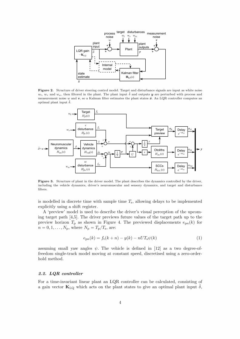
The structure of the parametric model is shown in Figure 2. The plant describesthe system controlled by the driver, including the vehicle dynamics and the driver’sneuromuscular dynamics and sensory systems. The driver’s control strategy followsthe linear quadratic Gaussian (LQG) framework, combining a linear quadratic reg-ulator (LQR) with a Kalman filter to give statistically optimal control actions andstate estimates based on the driver’s internal model of the plant. Previous studieshave used an LQR controller to model driver steering control while following a targetpath [4,5], hypothesising that an experienced driver will learn to steer in an approx-imately optimal fashion. Various studies have found evidence that humans combinevisual and vestibular information optimally [17–19], and humans have been found touse internal models to assist with motor control tasks [20]. A Kalman filter uses aninternal model to achieve optimal state estimation in the presence of additive whitenoise. Sections 2.1 to 2.4 describe the various components of the driver model; a fullmathematical derivation is presented in [12].

2.1. Plant

The plant describing the dynamics of the system controlled by the driver is shownin Figure 3. The driver’s internal model is assumed to be a perfect representationof the true plant. The plant input δ plus process noise w is filtered by the driver’sneuromuscular dynamics, giving the steering angle δ. Forcing functions ft, fv andfω are generated by filtering white noise plant inputs wt, wv and wω, and addedto the vehicle’s lateral velocity v and angular velocity ω. The driver previews theupcoming target ft, with measurements delayed by a visual delay τvi to give perceiveddisplacements evi. The vehicle lateral acceleration and angular velocity are sensedthrough the otoliths and semi-circular canals (SCCs), with a vestibular delay of τve inboth cases, giving perceived lateral acceleration ave and angular velocity ωve. The plant

3

Kalman filter HKF(s)

LQR gain−KLQ

Internal model

Plant

plantoutputs

measurement noise

+

+

state estimate

process noise

+

+

target disturbances

x

δ y

plant input

w

wt wv wωv

^

^

Figure 2. Structure of driver steering control model. Target and disturbance signals are input as white noise

wt, wv and wω , then filtered in the plant. The plant input δ and outputs y are perturbed with process and

measurement noise w and v, so a Kalman filter estimates the plant states x. An LQR controller computes anoptimal plant input δ.

Neuromusculardynamics

Hnm (s)

TargetHf t (s)

vdisturbance

Hfv (s)

ωdisturbance

Hfω (s)

Vehicledynamics

HVM(s)

Targetpreview

OtolithsHoto (s)

SCCsHSCC (s)

Delaye−sτvi

Delaye−sτve

Delaye−sτve

1s

sU

1s

y

ψ

fω

fv

ft

ωω^

vv^

δδ+w^

wt

wv

wω

evi

ave

ωve

+

+

++

+

+

ep

y

Figure 3. Structure of plant in the driver model. The plant describes the dynamics controlled by the driver,including the vehicle dynamics, driver’s neuromuscular and sensory dynamics, and target and disturbance

filters.

is modelled in discrete time with sample time Ts, allowing delays to be implementedexplicitly using a shift register.

A ‘preview’ model is used to describe the driver’s visual perception of the upcom-ing target path [4,5]. The driver previews future values of the target path up to thepreview horizon Tp as shown in Figure 4. The previewed displacements epn(k) forn = 0, 1, . . . , Np, where Np = Tp/Ts, are:

epn(k) = ft(k + n)− y(k)− nUTsψ(k) (1)

assuming small yaw angles ψ. The vehicle is defined in [12] as a two degree-of-freedom single-track model moving at constant speed, discretised using a zero-order-hold method.

2.2. LQR controller

For a time-invariant linear plant an LQR controller can be calculated, consisting ofa gain vector KLQ which acts on the plant states to give an optimal plant input δ,

4

y(k)

x

y

UTs

UTs

ft (k+1)

ft (k+Np)

ep0(k)ep1(k)

ep2(k)

epNp(k)

ψ(k)

ft (k)ft (k+2)

Figure 4. Model of the driver’s visual preview of the target path. The driver measures lateral displacementsof the target path relative to a line projected forward from the vehicle. Measurements are taken at intervals of

UTs up to a prediction horizon Np = Tp/Ts time steps ahead.

which minimises a cost function J . Additive white noise does not affect the optimalsolution, so the white noise plant inputs w, wt, wv and wω can be ignored. The costfunction incorporates costs on the tracking error ep0 and the plant input δ, weightedby qe and qδ:

J =

∞∑k=0

{qeep0(k)2 + qδ δ(k)2

}(2)

Previous studies have included costs on yaw angle error [4,5], and it is also possibleto add additional terms such as steering velocity to the cost function. However forsimplicity only two costs are included. The optimal solution only depends on therelative weightings, therefore qe is set to 1 m−2. As the steering cost is placed on δrather than δ, the cost on steering inputs is shaped by the neuromuscular transferfunction Hnm(s). The optimal gain KLQ can be found using the Matlab function dlqr.

2.3. Kalman filter

The LQR gain KLQ multiplies the plant states x(k) to give an optimal plant input δ.However, the driver only has access to measurements of the plant outputs y, perturbedby process and measurement noise w and v. Therefore, a Kalman filter is used tocompute an optimal estimate of the plant states based on the computed plant inputand noisy measurements of the plant outputs. The noise covariance matrices are givenby:

QKF = diag([W 2 W 2

v W 2ω W 2

t

])(3)

RKF = diag([V 2

p × 1(1, Np+1) V 2a V 2

ω

])(4)

where W 2, W 2v , W 2

ω and W 2t are the variances of the process noise w and the distur-

bance and target white noise inputs wv, wω and wt; V2

p , V 2a , and V 2

ω are the variancesof the measurement noise added to the plant outputs evi, ave, and ωve; and 1(1, Np+1)

is a column vector of (Np + 1) ones.

5

This model assumes that the measurement noise has the same variance for all pre-viewed target path displacements evi. Previous studies have accounted for an increasein noise with distance from the observer and eccentricity from the gaze direction [6],however there is a lack of research into how drivers view the geometry of an upcomingtarget path. The assumption of constant measurement noise Vp across all previeweddisplacements, while clearly a simplification, is not found to affect the fit to experi-mental results significantly. A time-invariant Kalman filter HKF(s) can be calculatedfor this system using the Matlab function kalman. The state estimate x can then befound from:

x(s) = HKF(s){δ(s) y(s)

}T(5)

2.4. Model transfer functions and parameters

As explained in Section 1, previous studies reviewed in [13] have shown that mea-surements of sensory perception taken in passive conditions may not be applicableto active control tasks such as driving [7–11]. Therefore, most of the parameters ofthe model are found using an identification procedure to fit to experimental results.However, the forms of some of the transfer functions can be fixed using results fromthe literature. Models of the vestibular system are taken from [21]:

HSCC(s) =458.4s2

(80s+ 1)(5.73s+ 1)(6)

Hoto(s) =0.4(10s+ 1)

(5s+ 1)(0.016s+ 1)(7)

Drivers’ neuromuscular dynamics are approximated by a second-order filter:

Hnm(s) =ω2

nm

s2 + 2ζnmωnms+ ω2nm

(8)

Pick and Cole [22] studied drivers’ neuromuscular dynamics by applying torque dis-turbances to a steering wheel and found values of ωnm = 5.65 rad/s and ζnm = 0.43 fordrivers with relaxed arms and ωnm = 23.2 rad/s and ζnm = 0.24 with tensed arms. Itis unclear which is more appropriate for driver steering models, as drivers’ arms maybe partially tensed, therefore ωnm and ζnm are identified to fit experimental data.

The values of some of the remaining parameters, such as the vehicle dynamics andthe spectra and amplitudes of the forcing functions, are given by the experimentalconditions. However various other parameters values must be identified, including thesteering cost weight qδ, preview time Tp, the visual and vestibular delays τvi and τve,noise amplitudes W , Va, Vω and Vp, and neuromuscular parameters ωnm and ζnm. Ifthe driver previews the upcoming target path they should be able to compensate fortheir internal latencies to follow the target without any delay. However, preliminaryanalysis of the experimental results showed that drivers sometimes steered earlier thanexpected, as if they were following a ‘shifted’ version of the target ft. This could bebecause the drivers aligned a different part of the car with the target other thanthe centre of mass. An additional time constant Tt is therefore included to model thiseffect, such that the driver attempts to follow ft(t−Tt) rather than ft(t). In total thereare eleven parameters which are neither determined by the experimental conditions

6

nor fixed using results from the literature, and these are found using the identificationprocedure described in Section 4.

3. Steering control experiment

A model of driver steering behaviour based on the dynamics of human sensory systemsis presented in Section 2. To investigate how sensory information is used during driving,an experiment was carried out to provide data which can be used to identify valuesfor the parameters of this model. A similar parameter identification procedure haspreviously been used in [14] to fit the model to an experiment carried out by pilots ina flight simulator [15]. The new experiment was designed following similar principlesto measure driver steering control in a combined target-following and disturbance-rejection task. The experiment was carried out in a driving simulator, rather than areal vehicle on a test track, due to the control that this allows over the experimentalset-up. Driving simulators have limited available travel, so the vehicle motion is usuallyscaled down or filtered to fit within these physical limitations. This results in a conflictbetween the information perceived by the visual and vestibular systems. There is somedisagreement in the literature as to how sensory conflicts are perceived by humans [13].Therefore, to ensure that the drivers used their sensory systems in the simulator in thesame way as they would in a real vehicle, the vehicle motion was designed to fit withinthe simulator limits without any scaling or filtering. (A separate set of experiments wasperformed to investigate and model the effect of sensory conflicts on driver steeringbehaviour, these are reported in [23].)

3.1. Steering control task

The steering control task carried out in the experiment was the same as the taskdescribed by the model in Section 2 (shown in Figure 1). The vehicle moved at constantlongitudinal speed U and the drivers were asked to follow a target lateral displacementft as closely as possible. Disturbances fv and fω were added to the lateral velocity andyaw angular velocity of the vehicle as shown in Figure 3. The target and disturbanceforcing function signals ft, fv and fω were generated by filtering Gaussian white noiseto match the assumptions made in the driver model. White noise signals wt, wv andwω were generated in discrete time by choosing random numbers from a zero-meannormal distribution. The variances W 2

t , W 2v and W 2

ω of these signals were adjustedbetween trials, as discussed in Section 3.3.

The forcing functions were tuned during preliminary testing to ensure that theamplitudes were as large as possible without exceeding the simulator limits, and toensure that a large range of frequencies was included without becoming uncomfortablefor the driver. The spectrum of the target forcing function ft was defined by combininga high-pass filter, to attenuate low frequencies and ensure that the target path waswithin the simulator limits, with a low-pass filter to restrict the bandwidth of thetarget:

Hft(s) =

(s

s+ 0.1

)2( 2

s+ 2

)2

(9)

The spectra of fv and fω were chosen so that, in the absence of any steering, the ve-hicle’s lateral displacement y would have the same spectrum as ft. This was achieved

7

Time (s)5 10 15 20 25 30 35 400

-0.15

-0.1

-0.05

0

0.05

0.1

0.15

Late

ral d

ispl

acem

ent y

(m

)

ftfv filtered by (1/s)fω filtered by (U/s2)

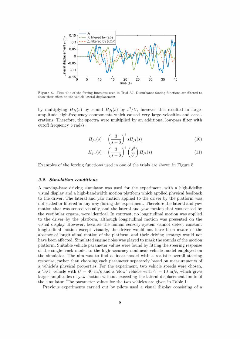
Figure 5. First 40 s of the forcing functions used in Trial A7. Disturbance forcing functions are filtered to

show their effect on the vehicle lateral displacement.

by multiplying Hft(s) by s and Hft(s) by s2/U , however this resulted in large-amplitude high-frequency components which caused very large velocities and accel-erations. Therefore, the spectra were multiplied by an additional low-pass filter withcutoff frequency 3 rad/s:

Hfv(s) =

(3

s+ 3

)2

sHft(s) (10)

Hfω(s) =

(3

s+ 3

)2(s2

U

)Hft(s) (11)

Examples of the forcing functions used in one of the trials are shown in Figure 5.

3.2. Simulation conditions

A moving-base driving simulator was used for the experiment, with a high-fidelityvisual display and a high-bandwidth motion platform which applied physical feedbackto the driver. The lateral and yaw motion applied to the driver by the platform wasnot scaled or filtered in any way during the experiment. Therefore the lateral and yawmotion that was sensed visually, and the lateral and yaw motion that was sensed bythe vestibular organs, were identical. In contrast, no longitudinal motion was appliedto the driver by the platform, although longitudinal motion was presented on thevisual display. However, because the human sensory system cannot detect constantlongitudinal motion except visually, the driver would not have been aware of theabsence of longitudinal motion of the platform, and their driving strategy would nothave been affected. Simulated engine noise was played to mask the sounds of the motionplatform. Suitable vehicle parameter values were found by fitting the steering responseof the single-track model to the high-accuracy nonlinear vehicle model employed onthe simulator. The aim was to find a linear model with a realistic overall steeringresponse, rather than choosing each parameter separately based on measurements ofa vehicle’s physical properties. For the experiment, two vehicle speeds were chosen,a ‘fast’ vehicle with U = 40 m/s and a ‘slow’ vehicle with U = 10 m/s, which giveslarger amplitudes of yaw motion without exceeding the lateral displacement limits ofthe simulator. The parameter values for the two vehicles are given in Table 1.

Previous experiments carried out by pilots used a visual display consisting of a

8

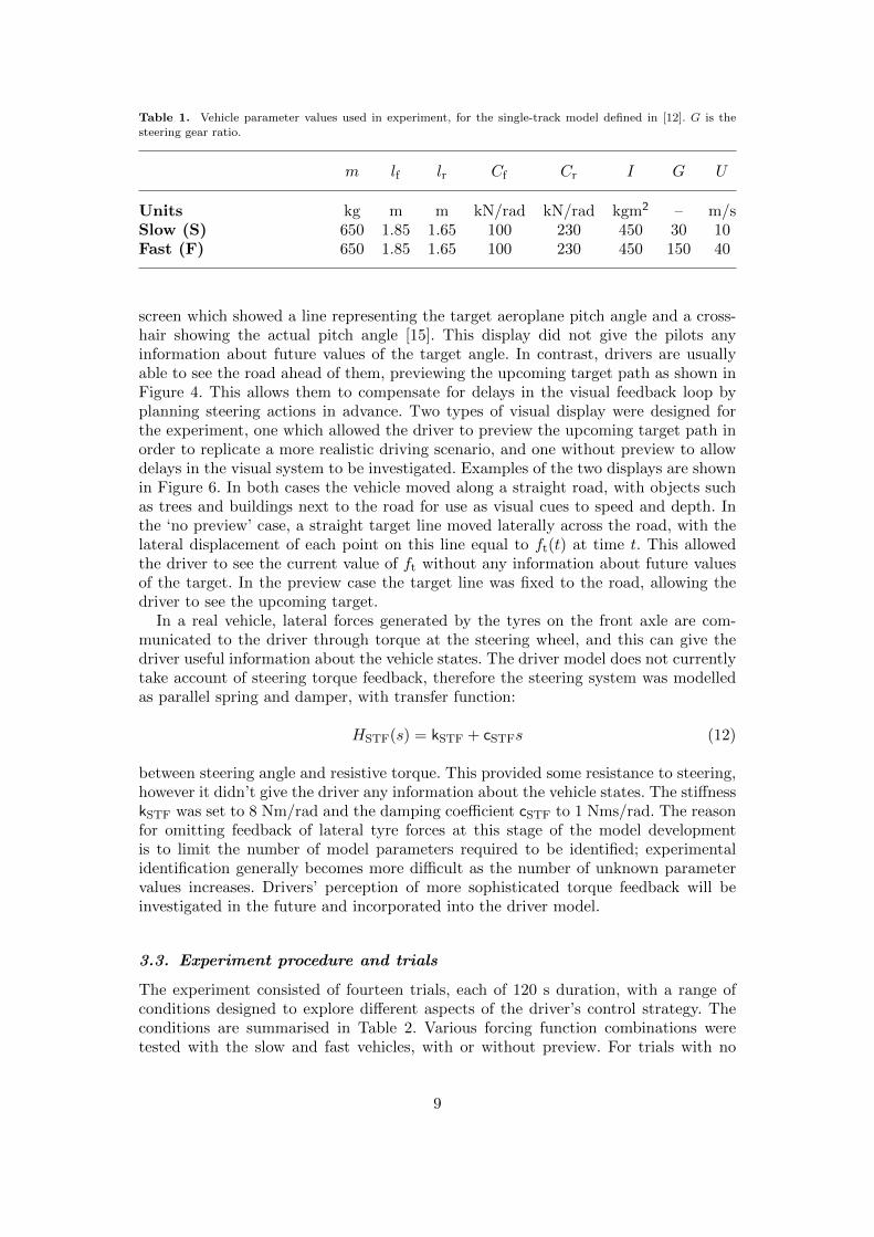
Table 1. Vehicle parameter values used in experiment, for the single-track model defined in [12]. G is the

steering gear ratio.

m lf lr Cf Cr I G U

Units kg m m kN/rad kN/rad kgm2 – m/sSlow (S) 650 1.85 1.65 100 230 450 30 10Fast (F) 650 1.85 1.65 100 230 450 150 40

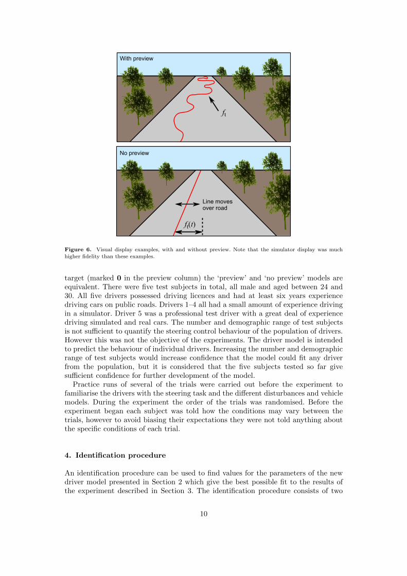
screen which showed a line representing the target aeroplane pitch angle and a cross-hair showing the actual pitch angle [15]. This display did not give the pilots anyinformation about future values of the target angle. In contrast, drivers are usuallyable to see the road ahead of them, previewing the upcoming target path as shown inFigure 4. This allows them to compensate for delays in the visual feedback loop byplanning steering actions in advance. Two types of visual display were designed forthe experiment, one which allowed the driver to preview the upcoming target path inorder to replicate a more realistic driving scenario, and one without preview to allowdelays in the visual system to be investigated. Examples of the two displays are shownin Figure 6. In both cases the vehicle moved along a straight road, with objects suchas trees and buildings next to the road for use as visual cues to speed and depth. Inthe ‘no preview’ case, a straight target line moved laterally across the road, with thelateral displacement of each point on this line equal to ft(t) at time t. This allowedthe driver to see the current value of ft without any information about future valuesof the target. In the preview case the target line was fixed to the road, allowing thedriver to see the upcoming target.

In a real vehicle, lateral forces generated by the tyres on the front axle are com-municated to the driver through torque at the steering wheel, and this can give thedriver useful information about the vehicle states. The driver model does not currentlytake account of steering torque feedback, therefore the steering system was modelledas parallel spring and damper, with transfer function:

HSTF(s) = kSTF + cSTFs (12)

between steering angle and resistive torque. This provided some resistance to steering,however it didn’t give the driver any information about the vehicle states. The stiffnesskSTF was set to 8 Nm/rad and the damping coefficient cSTF to 1 Nms/rad. The reasonfor omitting feedback of lateral tyre forces at this stage of the model developmentis to limit the number of model parameters required to be identified; experimentalidentification generally becomes more difficult as the number of unknown parametervalues increases. Drivers’ perception of more sophisticated torque feedback will beinvestigated in the future and incorporated into the driver model.

3.3. Experiment procedure and trials

The experiment consisted of fourteen trials, each of 120 s duration, with a range ofconditions designed to explore different aspects of the driver’s control strategy. Theconditions are summarised in Table 2. Various forcing function combinations weretested with the slow and fast vehicles, with or without preview. For trials with no

9

Line moves over road

ft(t)

ft

With preview

No preview

Figure 6. Visual display examples, with and without preview. Note that the simulator display was much

higher fidelity than these examples.

target (marked 0 in the preview column) the ‘preview’ and ‘no preview’ models areequivalent. There were five test subjects in total, all male and aged between 24 and30. All five drivers possessed driving licences and had at least six years experiencedriving cars on public roads. Drivers 1–4 all had a small amount of experience drivingin a simulator. Driver 5 was a professional test driver with a great deal of experiencedriving simulated and real cars. The number and demographic range of test subjectsis not sufficient to quantify the steering control behaviour of the population of drivers.However this was not the objective of the experiments. The driver model is intendedto predict the behaviour of individual drivers. Increasing the number and demographicrange of test subjects would increase confidence that the model could fit any driverfrom the population, but it is considered that the five subjects tested so far givesufficient confidence for further development of the model.

Practice runs of several of the trials were carried out before the experiment tofamiliarise the drivers with the steering task and the different disturbances and vehiclemodels. During the experiment the order of the trials was randomised. Before theexperiment began each subject was told how the conditions may vary between thetrials, however to avoid biasing their expectations they were not told anything aboutthe specific conditions of each trial.

4. Identification procedure

An identification procedure can be used to find values for the parameters of the newdriver model presented in Section 2 which give the best possible fit to the results ofthe experiment described in Section 3. The identification procedure consists of two

10

Table 2. Experimental conditions for each trial (data also appears in [23])

Forcing function amplitudes

Trial Wt (m*) Wv (m/s*) Wω (rad/s*) Vehicle Preview

A1 1.58 0 0 F 7A2 1.58 0 0 F 3A3 0 1.58 0 F 0A4 0 0 1.58 F 0A5 0 1.11 1.11 F 0A6 0.79 0.79 0.79 F 7A7 0.79 0.79 0.79 F 3A8 1.58 0 0 S 7A9 1.58 0 0 S 3A10 0 1.58 0 S 0A11 0 0 1.58 S 0A12 0 1.11 1.11 S 0A13 1.11 1.11 1.11 S 7A14 1.11 1.11 1.11 S 3

stages: Box–Jenkins identification to fit general polynomial transfer functions to theexperimental results; and parametric identification to find a set of parameter valuesfor the new driver model. The procedure is run separately for each of the five drivers.In addition, the measured steering angles are averaged over the five drivers to give aset of ‘averaged data’, which is also used for identification. The averaged data shouldcontain less random noise compared with the data for the individual drivers, allowingan average set of parameter values to be found more reliably. However, it relies on theassumption that the drivers were using similar control strategies. The first 15 s of eachtrial are excluded from the data used for identification, as the drivers may have takensome time to work out the conditions of the trial and settle on a control strategy.The final 30 s of each trial are also excluded, so that the fit of the last 30 s can bemeasured to validate the predictive power of the model and to check for over-fitting(see Section 5.2).

4.1. Box–Jenkins identification

The first identification stage involves fitting general transfer functions to the mea-sured data to estimate the contribution of linear control behaviour to the measuredsteering actions. This gives an approximate upper bound on how well the parametricdriver model could be expected to fit. The Box–Jenkins method is used to estimatepolynomial transfer functions between each of the model inputs (ft, fv, fω) and themodel output (δ) [24]. The method also finds a model of the noise spectrum Hn(s).Polynomial transfer functions of order 5 are used to give a good fit to the measure-ments without over-fitting [25]. The Box–Jenkins method can also make allowancesfor time delays between each input channel and the output, however the method doesnot estimate these directly from the data so they have to be known in advance. Tofind optimal values of these time delays, Box–Jenkins identification is carried out witha range of different delays and a genetic algorithm is used to iterate towards values

11

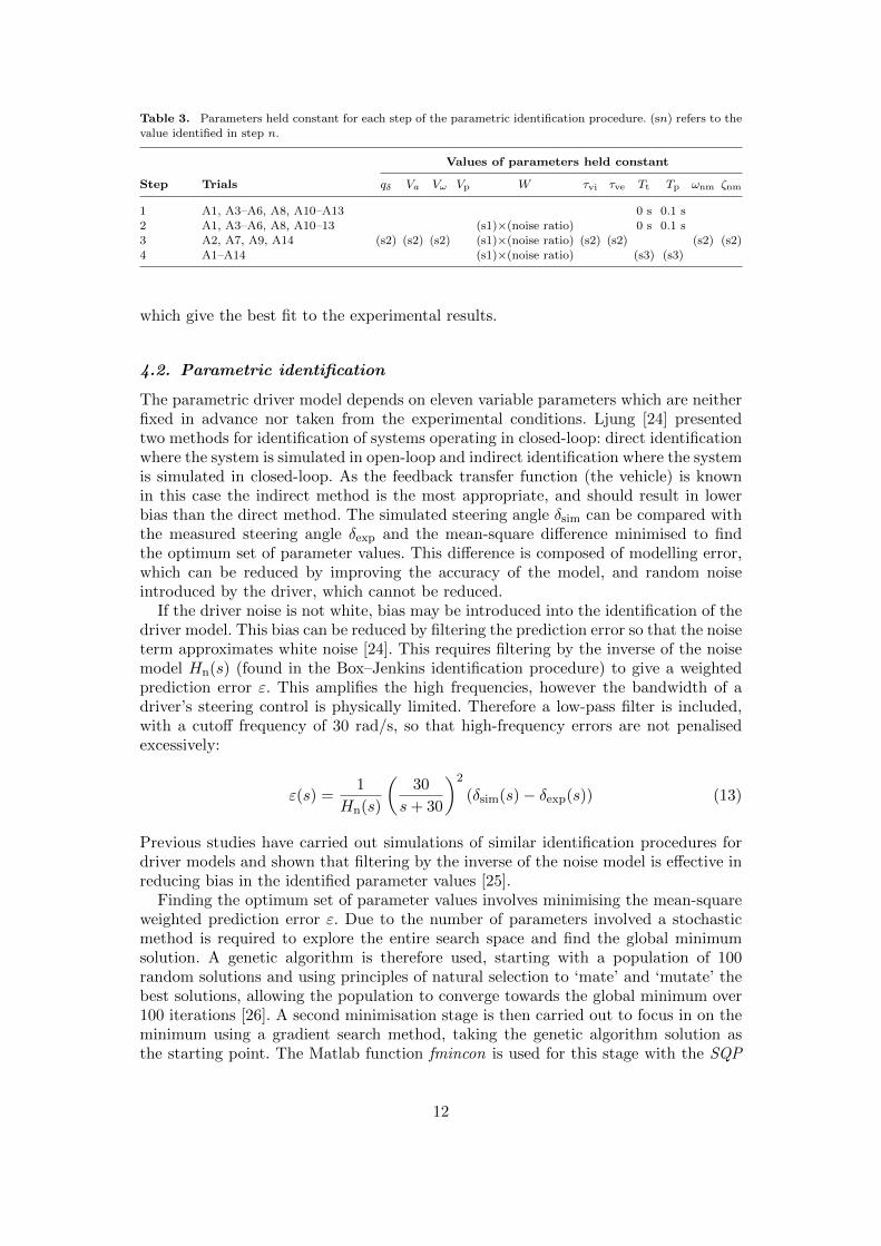
Table 3. Parameters held constant for each step of the parametric identification procedure. (sn) refers to the

value identified in step n.

Values of parameters held constant

Step Trials qδ Va Vω Vp W τvi τve Tt Tp ωnm ζnm

1 A1, A3–A6, A8, A10–A13 0 s 0.1 s

2 A1, A3–A6, A8, A10–13 (s1)×(noise ratio) 0 s 0.1 s

3 A2, A7, A9, A14 (s2) (s2) (s2) (s1)×(noise ratio) (s2) (s2) (s2) (s2)4 A1–A14 (s1)×(noise ratio) (s3) (s3)

which give the best fit to the experimental results.

4.2. Parametric identification

The parametric driver model depends on eleven variable parameters which are neitherfixed in advance nor taken from the experimental conditions. Ljung [24] presentedtwo methods for identification of systems operating in closed-loop: direct identificationwhere the system is simulated in open-loop and indirect identification where the systemis simulated in closed-loop. As the feedback transfer function (the vehicle) is knownin this case the indirect method is the most appropriate, and should result in lowerbias than the direct method. The simulated steering angle δsim can be compared withthe measured steering angle δexp and the mean-square difference minimised to findthe optimum set of parameter values. This difference is composed of modelling error,which can be reduced by improving the accuracy of the model, and random noiseintroduced by the driver, which cannot be reduced.

If the driver noise is not white, bias may be introduced into the identification of thedriver model. This bias can be reduced by filtering the prediction error so that the noiseterm approximates white noise [24]. This requires filtering by the inverse of the noisemodel Hn(s) (found in the Box–Jenkins identification procedure) to give a weightedprediction error ε. This amplifies the high frequencies, however the bandwidth of adriver’s steering control is physically limited. Therefore a low-pass filter is included,with a cutoff frequency of 30 rad/s, so that high-frequency errors are not penalisedexcessively:

ε(s) =1

Hn(s)

(30

s+ 30

)2

(δsim(s)− δexp(s)) (13)

Previous studies have carried out simulations of similar identification procedures fordriver models and shown that filtering by the inverse of the noise model is effective inreducing bias in the identified parameter values [25].

Finding the optimum set of parameter values involves minimising the mean-squareweighted prediction error ε. Due to the number of parameters involved a stochasticmethod is required to explore the entire search space and find the global minimumsolution. A genetic algorithm is therefore used, starting with a population of 100random solutions and using principles of natural selection to ‘mate’ and ‘mutate’ thebest solutions, allowing the population to converge towards the global minimum over100 iterations [26]. A second minimisation stage is then carried out to focus in on theminimum using a gradient search method, taking the genetic algorithm solution asthe starting point. The Matlab function fmincon is used for this stage with the SQP

12

algorithm.Initially, single sets of parameter values are identified for each driver to fit the

results of all trials. Minimisation over a multidimensional search space can be difficult,therefore the identification procedure is carried out in several steps to reduce thenumber of parameters identified at any one time. The conditions for each step are givenin Table 3. In step 1 parameter values are identified for the trials without preview,with Tt and Tp held constant at 0 and 0.1 s. Parameters W , Va, Vω and Vp affectnot only the linear component of the modelled control strategy, but also the predictedamplitude and distribution of the random noise introduced by the driver. It is desirablefor the noise amplitude predicted by the model to match the noise amplitude found inthe experiment. The modelling error is assumed to be small, so that the driver noiseis given by the difference between the measured steering angle δexp and the modelledsteering angle δsim. Simulations show that the predicted noise amplitude is affectedmuch more by the process noise than the measurement noise. Therefore, after step 1the average ratio of the measured to the modelled noise amplitudes is found and usedto scale W . In step 2, W is then held constant while the remaining parameter valuesare identified to fit the results of the non-preview trials once more.

In step 3, optimal values of Tt and Tp are found from the trials with preview. Thevalue of Vp is also allowed to vary, because the overall level of uncertainty in the visualmeasurements depends on the number of preview points. The target shift Tt was foundto be unnecessary for trials with the fast vehicle, so Tt is set to zero for trials A2 andA7. The other eight parameters are held constant at the values found in step 2. In step4 a further optimisation is carried out, holding Tt, Tp and W constant at the valuesfound previously and identifying the remaining eight parameter values to minimise theaverage weighted prediction error across all fourteen trials.

Once a single set of parameter values is found to fit all of the trials as well aspossible, separate parameter sets are identified for each trial individually. To reducethe number of parameters needing to be optimised, the values of Tp, Tt and W areheld constant, using the values found for the single parameter set. When running theparametric identification procedure for the averaged data, the value of W is given bythe average of the values identified for the separate drivers, to give a realistic predictednoise amplitude.

5. Results and analysis

In the following subsections, the results of the experiment and the identification pro-cedure are analysed in various ways. In Section 5.1 the agreement between the para-metric driver model and the results of the experiments is investigated. In Section 5.2the results are checked for signs of over-fitting to validate the model. The identifiedparameter values are compared between drivers in Section 5.3, and the noise levelspredicted using these parameters are compared with those found in the experiment inSection 5.4.

5.1. Agreement between model and measurements

It is possible to quantify the agreement between the measured and modelled steeringangles by calculating the ‘variance accounted for’ (VAF). This value represents thepercentage of the variance in the measured signals δexp which is matched by the model

13

Var

ian

ce A

ccou

nted

For

(%

)

0

20

40

60

80

100

Driver 1 Driver 2 Driver 3

Trial numberA0 A5 A10 A15

Var

ian

ce A

ccou

nted

For

(%

)

0

20

40

60

80

100

Driver 4

Trial numberA0 A5 A10 A15

Driver 5

Trial numberA0 A5 A10 A15

Averaged data

Box-Jenkins

Parametric (separateparameter sets)Parametric (singleparameter sets)

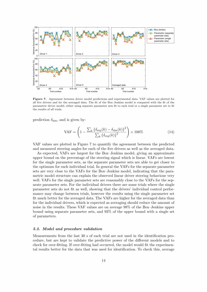
Figure 7. Agreement between driver model predictions and experimental data. VAF values are plotted forall five drivers and for the averaged data. The fit of the Box–Jenkins model is compared with the fit of the

parametric driver model, either using separate parameter sets fit to each trial or a single parameter set to fit

the results of all trials.

prediction δsim, and is given by:

VAF =

(1−

∑k {δexp(k)− δsim(k)}2∑

k {δexp(k)}2

)× 100% (14)

VAF values are plotted in Figure 7 to quantify the agreement between the predictedand measured steering angles for each of the five drivers as well as the averaged data.

As expected, VAFs are largest for the Box–Jenkins model, giving an approximateupper bound on the percentage of the steering signal which is linear. VAFs are lowestfor the single parameter sets, as the separate parameter sets are able to get closer tothe optimum for each individual trial. In general the VAFs for the separate parametersets are very close to the VAFs for the Box–Jenkins model, indicating that the para-metric model structure can explain the observed linear driver steering behaviour verywell. VAFs for the single parameter sets are reasonably close to the VAFs for the sep-arate parameter sets. For the individual drivers there are some trials where the singleparameter sets do not fit as well, showing that the drivers’ individual control perfor-mance may change between trials, however the results using the single parameter setfit much better for the averaged data. The VAFs are higher for the averaged data thanfor the individual drivers, which is expected as averaging should reduce the amount ofnoise in the results. These VAF values are on average 98% of the Box–Jenkins upperbound using separate parameter sets, and 93% of the upper bound with a single setof parameters.

5.2. Model and procedure validation

Measurements from the last 30 s of each trial are not used in the identification pro-cedure, but are kept to validate the predictive power of the different models and tocheck for over-fitting. If over-fitting had occurred, the model would fit the experimen-tal results better for the data that was used for identification. To check this, average

14

Table 4. Average VAFs for signals between (a) 15–90 s and (b) 90–115 s

Parametric ParametricBox–Jenkins (separate) (single)

Driver (a) (b) (a) (b) (a) (b)

1 76.6 69.7 71.1 64.7 59.7 59.62 81.1 80.6 79.3 78.3 70.8 71.73 74.0 71.2 70.6 66.3 64.0 61.84 64.2 68.3 59.5 63.7 52.4 58.05 79.2 72.4 77.2 66.6 69.7 63.6Averaged data 88.6 88.8 86.6 86.2 81.8 83.4

VAF values are calculated over all the trials for each driver, either for (a) the sig-nals between 15 s–90 s (which are used for identification) or (b) the signals between90 s–115 s. The results are compared for all three models in Table 4.

Table 4 shows evidence of some over-fitting in the Box–Jenkins results and theresults for the separate parameter sets, as the average VAF is lower in the final 30 sfor all drivers except driver 4 using these models. This is not seen for the averageddata, showing that the reduction in driver noise when averaging the measurementsreduces the level of over-fitting. These results show that the VAFs given in Figure 7for the Box–Jenkins model and single parameter sets may include a portion which isspuriously fitting to random variations in each trial. It also indicates that the separateparameter sets found for each trial may not always be reliable. In contrast, the resultsfor the single parameter sets do not show any evidence of over-fitting. VAFs are lowerin the last 30 s for drivers 3 and 5, but higher for drivers 2 and 4 and very similar fordriver 1. This shows that by optimising over all of the trials any random variationsare evened out, allowing a single set of parameter values to be found without fittingto noise in the results.

Simulated measurements were used to check that the identification procedure de-scribed reliably converges to the correct parameter values. Representative steeringangles were created for each trial using the driver model with the parameter valuesidentified for the averaged data over all trials. Measurement and process noise wereadded with the identified amplitudes, to give results with similar noise levels to the realmeasurements. An ensemble of ten sets of simulated results for each trial was createdwith different random noise signals, and the identification procedure was run for eachset. The resulting identified parameter values demonstrated that in general the pro-cedure does reliably converge to the correct parameter values. There was some slightvariation, as to be expected when the measurements contain a significant amount ofnoise, however the identified parameters did not deviate substantially from their truevalues.

5.3. Identified parameter values

A comparison of the single parameter sets identified for each of the drivers is shownin Figure 8. In general the parameter values are similar between the different drivers,showing that the drivers were using similar control strategies. The parameter valuesfound using the averaged data all fall within the range of the parameter values found

15

Ste

erin

g co

st qδ

(rad

-2*)

0

0.2

0.4

0.6

a no

ise

Va

(m/s

2 *)

0

0.2

0.4

0.6

0.8

1

ω n

oise

Vω

(ra

d/s*

)

0

0.02

0.04

0.06

0.08

Vis

ual n

ois

e Vp

(m)

0

1

2

3

Pro

cess

noi

se W

(ra

d*)

0

0.2

0.4

0.6

Pre

view

tim

e Tp

(s)

Driver number0 2 4 6

0

0.5

1

1.5

Ves

tibul

ar

dela

y τ ve

(s)

0

0.1

0.2

0.3

Vis

ual d

ela

y τ vi (

s)

0

0.1

0.2

0.3

Targ

et s

hift

Tt (

s)

Driver number0 2 4 6

-0.6

-0.4

-0.2

0

NM

freq

uen

cy ωnm

(ra

d/s)

Driver number0 2 4 6

0

10

20

30

40

NM

dam

ping

ζnm

Driver number0 2 4 6

0

0.5

1

1.5

2

Both vehicles

Averaged data

Fast (F) vehicle

Averaged data (F)

Slow (S) vehicle

Averaged data (S)

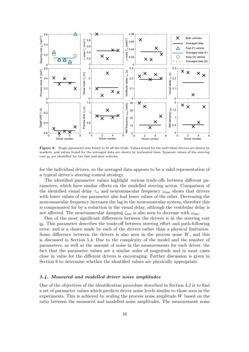
Figure 8. Single parameter sets found to fit all the trials. Values found for the individual drivers are shown bymarkers, and values found for the averaged data are shown by horizontal lines. Separate values of the steering

cost qδ are identified for the fast and slow vehicles.

for the individual drivers, so the averaged data appears to be a valid representation ofa typical driver’s steering control strategy.

The identified parameter values highlight various trade-offs between different pa-rameters, which have similar effects on the modelled steering action. Comparison ofthe identified visual delay τvi and neuromuscular frequency ωnm shows that driverswith lower values of one parameter also had lower values of the other. Decreasing theneuromuscular frequency increases the lag in the neuromuscular system, therefore thisis compensated for by a reduction in the visual delay, although the vestibular delay isnot affected. The neuromuscular damping ζnm is also seen to decrease with ωnm.

One of the most significant differences between the drivers is in the steering costqδ. This parameter describes the trade-off between steering effort and path-followingerror, and is a choice made by each of the drivers rather than a physical limitation.Some difference between the drivers is also seen in the process noise W , and thisis discussed in Section 5.4. Due to the complexity of the model and the number ofparameters, as well as the amount of noise in the measurements for each driver, thefact that the parameter values are a similar order of magnitude and in most casesclose in value for the different drivers is encouraging. Further discussion is given inSection 6 to determine whether the identified values are physically appropriate.

5.4. Measured and modelled driver noise amplitudes

One of the objectives of the identification procedure described in Section 4.2 is to finda set of parameter values which predicts driver noise levels similar to those seen in theexperiments. This is achieved by scaling the process noise amplitude W based on theratio between the measured and modelled noise amplitudes. The measurement noise

16

RM

S n

ois

e ex

perim

ent

/mo

del Driver 1

Driver 2Driver 3Driver 4Driver 5

Trial numberA0 A5 A10 A15

0.4

0.8

1.2

1.6

2

0

(a) Constant value of W

Driver 1Driver 2Driver 3Driver 4Driver 5

RM

S n

ois

e ex

peri

me

nt/m

ode

l

0.4

0.8

1.2

1.6

2

0

Trial numberA0 A5 A10 A15

(b) Adjusted values of W

RMS steering angle (rad)

Pro

cess

noi

se W

(ra

d*)

0 0.1 0.2 0.3 0.4 0.50

0.2

0.4

0.6

0.8

Driver 1Driver 2Driver 3Driver 4Driver 5

(c) W vs. RMS(δ)

Figure 9. Ratio of measured and modelled RMS driver noise amplitudes. In (a), a constant value of W is

used for each driver, whereas in (b) the values of W have been adjusted for each trial to match the noise levelsmore closely. In (c) adjusted values of W are plotted against RMS steering angle δ.

17

amplitudes Va, Vω and Vp are not scaled; while the Kalman filter is able to reducethe effects of measurement noise by using other measurements and an internal modelof the system, the process noise is added immediately before the plant so cannot bereduced as effectively by the driver. Simulations confirm that most of the noise in themodelled steering action originates from the process noise.

Assuming small modelling error, the driver noise is defined as (δsim−δexp). The ratiobetween the measured and modelled RMS noise amplitudes is shown in Figure 9a, usingthe single parameter sets identified for each driver. On average the noise amplitudesmatch well between the model and the experiment, with a ratio close to 1. There is areasonable amount of variation between trials, with the experimental noise generallylarger for the trials with the slow vehicle (A8–A14). To investigate the reasons behindthe variation in noise amplitudes across the different trials, the values of W are scaledby the ratio of the experimental to the modelled RMS noise amplitudes (as shown inFigure 9a) for each trial, and the simulations are run again. The agreement betweenthe measured and simulated steering angles is not affected, with the VAFs using theadjusted values of W on average 0.4% higher than the VAFs using a constant value ofW . The resulting ratios between measured and modelled noise amplitudes are shownin Figure 9b. These ratios are much closer to 1 than those found using constant Wvalues in Figure 9a.

The adjusted values of W are plotted against the RMS steering angle for each trialin Figure 9c. There is a clear linear relationship, showing that process noise is signal-dependent rather than additive. The amplitude RMS(δ) of steering actions applied bythe driver varies between trials and depends on the task and the driver’s internal costfunction. Therefore it may be more appropriate to define a constant signal-to-noiseratio (SNR) RMS(δ)/W between the RMS steering angle and the RMS process noise,rather than a constant value of W . Figure 9c shows that the SNRs are similar betweenthe different drivers, with a value of 0.57 on average.

6. Discussion

The results presented in Section 5 can be used to give an insight into driver steer-ing control behaviour and sensory systems during a realistic driving task, allowingknowledge of the underlying mechanics of human perception to be combined withunderstanding of the higher-level control strategies used while driving.

6.1. General discussion of results

Experimental data has been used to identify parameter values for a parametric drivermodel based on a physical understanding of human sensory dynamics. The VAF valuespresented in Section 5.1 show that the parametric model fits the experimental resultsalmost as well as the upper bound given by the Box–Jenkins model. This result sup-ports the hypothesis that driver steering control can be predicted using models ofthe underlying sensory mechanisms. The parametric model fits the results of all trialswell with a single fixed set of parameter values. Simplifications have been made in themodelling of human sensory dynamics, such as neglecting visual perception of vehiclemotion and assuming constant measurement noise on each previewed lateral displace-ment. The good agreement between the parametric model and experimental resultsshows that these assumptions are reasonable.

Another assumption made in the model is that the measurement and process noise is

18

Table 5. Comparison of identified parameter values with estimates from literature. Identified values are found

using the averaged data.

Parameter qδ (fast) qδ (slow) Va Vω Vp W τvi τve Tt Tp ωnm ζnm

Units rad−2* rad−2* m/s2* rad/s* m rad* s s s s rad/s –

Identified 0.13 0.087 0.46 0.033 1.1 0.32 0.16 0.19 -0.55 0.85 10 0.54Literature – – 0.038 0.023 – – 0.10–0.56 0.05–0.44 – 1 5.65–23.2 0.24–0.43

Gaussian, white and additive. In Section 5.4 the process noise W is found to correlatelinearly with RMS steering angle, indicating that process noise is signal-dependentrather than additive. Signal-dependent noise could be included explicitly in the drivermodel [6], however this increases the complexity and computational requirements sincethe standard LQR and Kalman filter solutions are no longer optimal. As long as theconditions do not vary significantly over time a simpler solution is to choose additivenoise amplitudes based on the expected average signal amplitudes.

Parameter values identified for each of the five drivers are found in Section 5.3to be similar in general. No significant differences are found between a professionaldriver (driver 5) and normal drivers. This could be because the identified delays andnoise amplitudes are linked to physical limitations which are similar in most healthyhumans, so for simple tasks like those carried out in the experiment more experienceddrivers do not necessarily have any advantage. The advantage of a professional driveris likely to be more apparent in the nonlinear handling regime near the limit of tyreadhesion, and in planning the optimum target trajectory.

6.2. Comparison of parameter values with literature results

A review of relevant literature relating to sensory dynamics during driving was carriedout in [13], allowing the identified parameter values to be compared with results fromthe literature to determine whether the parametric driver model gives a realistic de-scription of the function of sensory systems during driving. A comparison between thesingle set of parameter values identified to fit the averaged data and estimates fromthe literature is presented in Table 5.

There is some disagreement in the literature as to the values of delays in the visualand vestibular systems, and it can be difficult to distinguish between pure delays,lags and time taken to overcome threshold levels. Transmission of vestibular reflexsignals has been found to be very fast [27], however other studies have suggestedthat neural processing of vestibular information may take longer than processing ofvisual information [28]. The identified vestibular delay of 0.19 s is slightly longer thanthe visual delay of 0.16 s, supporting the hypothesis that processing of vestibularinformation takes longer than visual information. Both of these values are within the(somewhat large) range suggested by results from the literature, and they can be usedas a more specific estimate of sensory delays during driving.

Soyka et al. [29] developed a signal-in-noise model of sensory thresholds, whichcan be used to infer noise amplitudes from measured threshold data. Estimated noiseamplitudes using this approach are compared with identified values in Table 5. Theidentified value of Vω is 1.4 times the value found from sensory threshold measure-ments, whereas the identified value of Va is 12 times larger. Studies have found thatvestibular thresholds may increase by factors between 1.5 and 6 during an active con-trol task [7–10], which can explain the larger value of Vω but not of Va. However, whilethe angular velocities in the experiment were very small and close to threshold levels,

19

the accelerations were much larger than the perception threshold. The ‘just noticeabledifference’ for accelerations increases with stimulus amplitude [30], so the identifiednoise amplitude Va may include signal-dependent as well as additive noise. Taking thisinto account, the identified noise amplitudes are plausible.

Studies measuring drivers’ gaze direction have found that drivers tend to lookaround 1 s ahead [3,31,32]. The identified preview time Tp is 0.85 s, which is slightlyshorter than the 1 s found in the literature. This may be a result of the small targetlateral displacements and the assumption of constant visual noise Vp, when in realitythe target would become more difficult to see as the preview distance increases. Theidentified target shift Tt (which is only used for the slow vehicle) is 0.55 s, implyingthat the drivers steered 5.5 m ahead of the target on average. They may have alignedthe front of the vehicle with the target rather than the centre of mass, although thiscannot account for the full distance. Another explanation is that at low speeds theassumption of constant preview time could be invalid, and drivers look further aheadso that the preview distance isn’t too short.

The identified neuromuscular frequency ωnm is between values found for relaxedand tensed arms [22], however the identified damping ratio ζnm is higher than thevalues found in both cases. In reality the driver’s neuromuscular system interacts inclosed-loop with the spring-damper torque feedback of the steering wheel, howeverthis interaction is not captured in the model. Therefore, the identified neuromusculartransfer function incorporates this complete closed-loop system, which acts as a low-pass filter between δ and δ. While the transfer function for the neuromuscular dynamicsin the model is intended to correspond to the dynamics of the driver’s arm muscles, italso plays a role in shaping the cost function. The steering cost is applied to δ, based onthe hypothesis that the driver aims to minimise control inputs to the neuromusculardynamics. However, the driver may have other costs, for example derivatives or filteredversions of δ, and these may come across in the identified neuromuscular parametervalues.

Overall, comparison of the identified sensory parameter values with values foundin the literature shows the identified values to be physically plausible. Although theidentified noise amplitudes are larger than values inferred from sensory threshold mea-surements, this aligns with expectations during an active control task with multimodalsensory stimuli. The aim of the parametric driver model is to predict driver steeringbehaviour based on considerations of the physiological processes involved, so it is en-couraging that the identified parameter values give a reasonable description of humansensory systems.

6.3. Implications and limitations

A model of driver steering control has been developed based on an optimal controlstrategy, incorporating models of the driver’s sensory dynamics. The model fits exper-imental results well, and identified sensory parameters are physically plausible whencompared with measurements from the literature. These results support the hypothesisthat drivers achieve close to the best possible control performance within the limita-tions of their sensory and motor systems. Experienced drivers will have spent manyhours driving, allowing them to learn how best to use sensory information to control avehicle. Increasing the number and demographic range of test subjects would increaseconfidence that the model could fit any driver from the population, but it is consideredthat the five subjects tested so far give sufficient confidence for further development

20

of the model.The model gives a physical basis for the driver’s control decisions which is lacking

in many existing models. Furthermore, this work has more general implications forthe understanding of neuronal information processing during active control tasks. Theidentified time delays and noise parameters give an insight into the limitations of hu-man sensorimotor systems in such a task, and how they compare with previous studieswhich have generally taken measurements under controlled, passive conditions. It isalso shown that the processing carried out in the brain during an active control tasksuch as driving can be modelled reliably by an optimal controller and state estimator.

The driver model presented in this paper has several limitations. The model is onlyderived for constant speed vehicles, and the yaw angle of the vehicle is assumed to besmall. A linear vehicle model is used, which is a reasonable approximation for regulardriving, however under more extreme conditions drivers may operate in the nonlinearregion close to the limit of adhesion of the tyres. Driving simulator experiments withvarying vehicle speed and nonlinear tyres may reveal greater differences in controlbehaviour between drivers than observed in the present experiments. The current op-timal control approach to modelling the driver will likely require extension to representthe measured behaviour and differences between drivers. Nonlinear model predictivecontrol is one possibility [12] but account may also need to be taken of non-optimalbehaviour when the driver has not fully learnt the vehicle dynamics.

The current model is derived for random targets and disturbances, however furtherwork is necessary to determine how drivers deal with more predictable or transientconditions. The derivation of the driver model assumes that there are no conflictsbetween the senses, and the experiment was carefully designed to allow the vehiclemotion to be replicated at full scale. However, it is necessary to investigate how driversbehave when there are sensory conflicts, in particular when the motion is scaled orfiltered. These limitations are addressed in further work [23].

7. Conclusion

A parametric model of driver steering control has been developed, incorporating hu-man sensory dynamics and hypothesising that the driver’s control strategy is close tooptimal within the limitations of their sensory and motor systems. Model predictionsmatch experimental results from five test subjects well, with a ‘variance accountedfor’ on average 98% of the upper bound on linear behaviour using separate parametersets for each trial, and 93% of the upper bound with a single fixed parameter set. Theidentified parameter values are physically plausible compared with values from theliterature. Identified vestibular delays are longer than visual delays, supporting previ-ous studies which have suggested that processing of vestibular information takes longerthan visual information. The identified process noise amplitudeW is linearly correlatedwith the RMS steering angle δ, showing that process noise is signal-dependent. Thesignal-to-noise ratio RMS(δ)/W is consistent across the different trials and drivers,at around 0.57. Differences between the test subjects mainly resulted from differentcost function weightings, and similar parameter values are identified for a professionaldriver to those found for less experienced drivers. Further work is necessary to addressthe limitations of the current model, considering nonlinear vehicles, more realistic roadprofiles and the effects of sensory conflicts on a driver’s control performance.

21

Acknowledgement and data

This work was supported by the UK Engineering and Physical Sciences ResearchCouncil (EP/P505445/1, studentship for Nash). Supporting data are available atdoi.org/10.17863/CAM.1244.

References

[1] MacAdam CC. Understanding and Modeling the Human Driver. Vehicle System Dynam-ics. 2003;40(1-3):101–134.

[2] Plochl M, Edelmann J. Driver models in automobile dynamics application. Vehicle SystemDynamics. 2007;45(7-8):699–741.

[3] Donges E. A Two-Level Model of Driver Steering Behavior. Human Factors: The Journalof the Human Factors and Ergonomics Society. 1978;20(6):691–707.

[4] Sharp RS, Valtetsiotis V. Optimal preview car steering control. Vehicle System Dynamics.2001;35(Suppl.1):101–117.

[5] Cole DJ, Pick AJ, Odhams AMC. Predictive and linear quadratic methods for poten-tial application to modelling driver steering control. Vehicle System Dynamics. 2006;44(3):259–284.

[6] Bigler RS. Automobile Driver Sensory System Modeling Phd thesis. Cambridge Univer-sity; 2013.

[7] Pool DM, Valente Pais AR, De Vroome AM, et al. Identification of Nonlinear MotionPerception Dynamics Using Time-Domain Pilot Modeling. Journal of Guidance, Control,and Dynamics. 2012;35(3):749–763.

[8] Valente Pais AR, Pool DM, De Vroome AM, et al. Pitch Motion Perception ThresholdsDuring Passive and Active Tasks. Journal of Guidance, Control, and Dynamics. 2012;35(3):904–918.

[9] Groen EL, Bles W. How to use body tilt for the simulation of linear self motion. Journalof vestibular research : equilibrium & orientation. 2004;14(5):375–385.

[10] Rodchenko V, Boris S, White A. In-flight estimation of pilots’ acceleration sensitivitythresholds. In: Modeling and Simulation Technologies Conference; Reston, VA. AmericanInstitute of Aeronautics and Astronautics; 2000. p. e4292.

[11] Groen E, Wentink M, Valente Pais A, et al. Motion Perception Thresholds in FlightSimulation. In: AIAA Modeling and Simulation Technologies Conference and Exhibit;Reston, VA. American Institute of Aeronautics and Astronautics; 2006. p. e6254.

[12] Nash CJ, Cole DJ. Modelling the influence of sensory dynamics on linear and nonlineardriver steering control. Vehicle System Dynamics. 2018;56(5):689–718.

[13] Nash CJ, Cole DJ, Bigler RS. A review of human sensory dynamics for application tomodels of driver steering and speed control. Biological Cybernetics. 2016;110(2-3):91–116.

[14] Nash CJ, Cole DJ. Development of a novel model of driver-vehicle steering control in-corporating sensory dynamics. In: Rosenberger M, Plochl M, Six K, et al., editors. Thedynamics of vehicles on roads and tracks. Graz, Austria: CRC Press; 2016. p. 57–66.

[15] Zaal PMT, Pool DM, Mulder M, et al. Multimodal Pilot Control Behavior in CombinedTarget-Following Disturbance-Rejection Tasks. Journal of Guidance, Control, and Dy-namics. 2009;32(5):1418–1428.

[16] Timings JP, Cole DJ. Minimum Maneuver Time Calculation Using Convex Optimization.Journal of Dynamic Systems, Measurement, and Control. 2013;135(3):031015.

[17] Butler JS, Smith ST, Campos JL, et al. Bayesian integration of visual and vestibularsignals for heading. Journal of Vision. 2010;10(11):23.1–13.

[18] Prsa M, Gale S, Blanke O. Self-motion leads to mandatory cue fusion across sensorymodalities. Journal of neurophysiology. 2012;108(8):2282–2291.

[19] Fetsch CR, Deangelis GC, Angelaki DE. Visual-vestibular cue integration for heading

22

perception: applications of optimal cue integration theory. The European journal of neu-roscience. 2010;31(10):1721–1729.

[20] Wolpert DM, Ghahramani Z. Computational principles of movement neuroscience. Natureneuroscience. 2000;3:1212–7.

[21] Telban RJ, Cardullo F. Motion cueing algorithm development: Human-centered linearand nonlinear approaches. NASA; 2005.

[22] Pick AJ, Cole DJ. Dynamic properties of a driver’s arms holding a steering wheel. Pro-ceedings of the Institution of Mechanical Engineers, Part D: Journal of Automobile En-gineering. 2007;221(12):1475–1486.

[23] Nash CJ, Cole DJ. Measurement and modelling of the effect of sensory conflicts on driversteering control. accepted for publication, Journal of Dynamic Systems, Measurement andControl. 2019;.

[24] Ljung L. System Identification: Theory for the User. 2nd ed. Upper Saddle River, NJ:Prentice Hall; 1999.

[25] Odhams AM, Cole DJ. Identification of the steering control behaviour of five test subjectsfollowing a randomly curving path in a driving simulator. International Journal of VehicleAutonomous Systems. 2014;12(1):44–64.

[26] Zaal PMT, Pool DM, Chu QP, et al. Modeling Human Multimodal Perception and Con-trol Using Genetic Maximum Likelihood Estimation. Journal of Guidance, Control, andDynamics. 2009;32(4):1089–1099.

[27] Aw ST, Todd MJ, Halmagyi GM. Latency and initiation of the human vestibuloocularreflex to pulsed galvanic stimulation. Journal of neurophysiology. 2006;96(2):925–930.

[28] Barnett-Cowan M. Vestibular perception is slow: a review. Multisensory research. 2013;26(4):387–403.

[29] Soyka F, Robuffo Giordano P, Beykirch KA, et al. Predicting direction detection thresh-olds for arbitrary translational acceleration profiles in the horizontal plane. Experimentalbrain research. 2011;209(1):95–107.

[30] Naseri AR, Grant PR. Human discrimination of translational accelerations. Experimentalbrain research. 2012;218(3):455–464.

[31] Land MF, Tatler BW. Steering with the head. Current Biology. 2001;11(15):1215–1220.[32] Chattington M, Wilson M, Ashford D, et al. Eye–steering coordination in natural driving.

Experimental Brain Research. 2007;180(1):1–14.

23