Identification of Driver Steering and Speed Controldjc13/vehicledynamics/downloads/Odhams_Ph… ·...
263
Identification of Driver Steering and Speed Control Andrew Murray Charles Odhams Queens’ College A dissertation submitted to the University of Cambridge for the Degree of Doctor of Philosophy Cambridge University Engineering Department September 2006
Transcript of Identification of Driver Steering and Speed Controldjc13/vehicledynamics/downloads/Odhams_Ph… ·...

Identification of Driver Steering
and Speed Control
Andrew Murray Charles Odhams
Queens’ College
A dissertation submitted to the University of Cambridge
for the Degree of Doctor of Philosophy
Cambridge University Engineering Department
September 2006

ii
To Nina

iii
Summary
This thesis addresses the modelling of driver steering control and speed choice during
road vehicle driving. Speed choice is an important factor in road accidents, and also in
driver learning. Driver steering control is an important factor in speed choice.
Improved understanding of speed choice could assist in the design of roads and
vehicles to aid more appropriate, and therefore safer, speed choice. Research into the
steering and speed choice behaviour of drivers was carried out to address this need.
Chapter one reviews previous literature relevant to driver speed choice. Literature
relating to driver steering control and system identification was also reviewed.
Chapter two addresses the modelling of speed choice by testing existing models
against simulator data, and assesses a path error based speed choice hypothesis by
examining a subject’s path error and speed choice during a simulator experiment. A
need to quantify driver steering strategy is identified, leading to the work of chapters
three, four and five.
Chapter three describes and compares driver steering models developed from Sharp’s
LQR steering model. These include simplified internal models for novice drivers, and
a model of the neuromuscular system.
Chapter four describes the design and validation of identification algorithms and
simulator experiments for the identification of driver preview models from closed
loop driver data.
Chapter five describes the results of this driver preview model identification from
measured simulator data comparing different driver preview models, test subjects,
speeds and road widths. Conclusions and recommendations for future work are given
in chapter six.
iv
Preface
A PhD research project was carried out between October 2002 and September 2006
aimed at identifying the speed choice and steering control of drivers. This work on
driver speed choice was funded by a research studentship from the Engineering and
Physical Sciences Research Council (EPSRC). Financial assistance was also given by
Queens’ College Cambridge. I would like to thank these organisations for their
support.
My thanks go to Dr David Cole, who originally proposed the project, and supervised
throughout. His help, advice and encouragement have been invaluable in the
completion of this work.
I would like to thank all of the test subjects, some of whom did not enjoy the tests at
all, and many of whom were not included in the final results. I would also like to
thank all the members of the MRO, DVRO, and other members of the DVRG past
and present who have made the duration of the project both more productive, and
more enjoyable. My thanks also go to the mechanics group technicians, who helped
to build the simulator hardware and gave much practical advice.
I would also like to thank my family and friends for their encouragement and support
throughout. My particular thanks go to Nina Pickett for her help and emotional
support.
This dissertation is my own work and contains nothing that is the outcome of work
done in collaboration with others, except as specified in the text and
acknowledgements. No part of the work has already been, or is currently being,
submitted for any degree, diploma or other qualification. This dissertation contains
46,024 words and 139 figures.
Andrew Odhams, September 2006

v
List of Notation [0/0] Noise model order [numerator order/denominator order]
A 2 DOF bicyle model state space matrix
dA Discretised A matrix
arg min ( ) x f x Value of x which minimises ( )f x
a Front axle to CG distance
( )B ω Identification bias term in Ljung’s derivation.
b Rear axle to CG distance
1 1,a b Constants for Felip & Navin’s model of speed choice
2 2,a b Constants for De Fazio’s model of speed choice
3 3,a b Constants for Bottoms’ model of speed choice
4 4 4 4, , ,a b c d Constants for surface model of speed choice
5 5 5 5, , ,a b c d Constants for lateral error vs. speed vs. curvature surface
7a Velocity offset for TLC model
B 2 DOF bicycle model state space matrix
dB Discretised B matrix
nmsB Neuromuscular system damping from Pick’s model of limb
dynamics
fC Front axle tyre cornering stiffness
rC Rear axle tyre cornering stiffness
C Road curvature
1C Transformation matrix for Sharp’s LQR model
maxC∆ Driver’s curvature margin in Reymond’s model
D Track shift register matrix in Sharp’s LQR model
E Input matrix for new point on track in Sharp’s LQR model
( )e t Driver steer angle white noise
( )F q Vehicle system as a linear transfer function
vi
IG , IIG , IIIG , IVG , VG ,
VIG , VIIG , VIIIG
Set of LQR driver models proposed in chapter 3
( )G q Driver LQR controller
'( )G q Estimate of driver LQR controller
( )H q Driver noise filter
'( )H q Estimate of driver noise filter (noise model)
{ }' ', ', 'yH q qθ τ Estimate of noise model based on identified parameters
{ }', ', 'yq qθ τ
I Vehicle yaw moment of intertia
nmsJ Neuromuscular system inertia in Pick’s model
J Cost function value
swK Steering wheel to front wheel angle gain
nmsK Neuromuscular system stiffness from Pick’s model
1K , 2K Parameters of Odhams’ speed adaptation model
k Ratio of steer angle error to steer angle from Reymond’s LCT
model
1k Constant in linearisation of Prokop’s steer model.
{ }pi Ik G Preview gains for model IG
( )Nd
k kδ δ… Steer angle delay state gains for model IVG
kω Yaw rate state gain in LQRk
kυ Sideslip state gain in LQRk
M Vehicle body mass
dN Number of delay states in model IVG
( )n t Vehicle position signal
'( )n t Estimated vehicle position signal
Q Matrix of lateral and heading error weights
in Sharp’s LQR model

vii
yq Lateral error weight in LQR cost function
for models IG to VIIIG
qθ Heading angle error weight in LQR cost function
for models IG to VIIIG
'yq , 'qθ Estimates of yq and qθ used in estimated driver model 'G
Gyq , Gqθ True values of yq and qθ used to generate dummy data for
identification validation in chapter 4.
{ }[1] 30'y Uq = Three 'yq values for subject 1 at 30U = m/s.
R Road curve radius
R∂ Curve radius error of driver in Reymond’s LCT model
( )r t Road path input signal
0pS Value of tS for track point perpendicular to the vehicle
( , )S ψ Vehicle path defined in intrinsic co-ordinates
( ),t tS ψ Track defined in intrinsic co-ordinates
T Time step of discrete LQR model formulation
LCT Time to lane crossing parameter.
dT Tracking difficulty in Bottoms’ model
( )demT s Torque applied to neuromuscular system through the steering
wheel
U Forward speed of vehicle
( )Uµ Mean forward speed of vehicle
( )ccUµ Mean of ccU
0U Maximum comfortable speed on straights
ccU U in constant radius part of 180° curve
( )u t Input signal to the driver
'( )u t Estimate of inputs ( )u t in indirect method where vehicle ( )F q
operates in closed loop with the estimated driver '( )G q
W Width of left hand lane of road, beyond which buzzers sound
vW Vehicle width

viii
1 2 3, ,W W W Weights for path error based speed choice hypothesis
[ ]vyν ω θ=vx Vector of vehicle velocity and position states used in derivation of
Sharp’s LQR controller.
( ),x y Position in global Cartesian co-ordinates
( ),x y Position in local driver Cartesian co-ordinates (centered on
Vehicle, and yawing with vehicle)
( )t tx , y Vector of discrete track points in global co-ordinates
( )t tx , y Vector of discrete track points in local driver co-ordinates
( ) ( )1 2,r r riy y y=ry … Vector of previewed lateral offsets in global co-ordinates
( ) ( )1 2,p p piy y y=py … Vector of previewed lateral offsets in local driver co-ordinates
vy Vehicle position state in vx
0py Vehicle lateral error from path.
z Vector of vehicle and track states joined
α Angle subtended to lane exit with radius error in Reymond’s LCT
model.
β Expedience parameter in Herrin and Neuhardt’s model.
Γ Lateral acceleration
∆Γ Lateral acceleration safety margin
ccΓ Lateral acceleration in constant radius part of 180° curve
maxΓ Driver prediction of maximum available lateral acceleration
γ Track angle PSD frequency roll-off parameter
fδ Front wheel angle of vehicle
( )tδ Driver steering wheel angle
'( )tδ Estimate of driver steering wheel angle
( )out tδ Driver steer angle output post NMS system
( )1,...,Ndδ δ− Delay states of steer angle for model IVG
ε Weighted steer angle prediction error ς Constant in Emmerson’s model of speed choice
( )tη Driver steer angle filtered noise ( )He t=

ix
θ Vehicle yaw angle
Θ Generalised effort parameter encompassing driver steering
strategy.
κ Track angle PSD amplitude parameter
λ Percentile of lateral error (0 to 100) 1Wλ Percentile of lateral error recorded for width 1W
1λ Damping in Odhams’ adaptation model
[1:5] ( ')qθµ , [1:5] ( ')yqµ ,
[1:5] ( ')nµ ω , [1:5] ( ')µ ξ
Mean of the estimates of yq , qθ , 'ξ and 'nω across 5 subjects
and 3 repetitions for each subject for a given speed
[1:5] ( ( ))µ υΞ Mean of ( )υΞ across 5 subjects and 3 repetitions for each subject
for a given speed.
( ', ')err yq qθµ Percentage error of mean of parameter estimates ( ', ')yq qθ from
their true values ( , )G Gyq qθ
ν Lateral speed of vehicle (sideslip)
(e)Ξ RMS of driver noise e(t)
( )ηΞ RMS of filtered driver noise (t)η
( )εΞ RMS of weighted steer angle prediction error ε
( )0eδ =Ξ RMS of steer angle of model IG driving road with no added noise
e .
( )υΞ RMS of unweighted steer angle prediction error υ
ξ Neuromuscular system damping factor
yΠ Ratio of 95th percentile steer angle to 95th
percentile lateral error
θΠ Ratio of 95th percentile steer angle to 95th
percentile yaw error
95 0( )pyρ 95th percentile lateral error
( ', ')err yq qθσ Standard deviation of parameter estimates ( ', ')yq qθ as a
percentage of their true values ( , )G Gyq qθ
τ Driver delay
'τ Estimate of driver delay τ used in estimated driver model 'G
x
Gτ True value of driver delay used to generate dummy data for
identification validation in chapter 4
υ Unweighted steer angle prediction error
( )r ωΦ Spectrum of road input ( )r t
( )u ωΦ Spectrum of driver input ( )u t
( )eu ωΦ Spectrum of input ( )u t resulting from driver noise ( )e t fed back
through vehicle. χ Wavenumber for definition of track angle PSD
tψ Track angle defined in intrinsic coordinates
piψ ith increment of track angle tψ in the vehicle reference frame
ω Yaw rate of vehicle
nω Natural frequency of 2nd order neuromuscular system model

xi
Contents Summary..................................................................................................................... iii
Preface..........................................................................................................................iv
List of Notation.............................................................................................................v
Contents .......................................................................................................................xi
Chapter 1: Review of driver speed choice and steering models..........................1
1.1 Introduction: Motivation for understanding speed choice .............................1
1.2 Models of speed choice..................................................................................4
1.2.1 Lateral acceleration................................................................................4
1.2.2 Available tolerance ................................................................................7
1.2.3 Path error models ...................................................................................9
1.2.4 Coupled models of steering and speed control ....................................13
1.2.5 Speed adaptation ..................................................................................13
1.2.6 Summary of speed choice ....................................................................18
1.3 Driver steering control .................................................................................20
1.3.1 Compensatory control..........................................................................20
1.3.2 Preview control ....................................................................................20
1.3.3 Neuromuscular systems .......................................................................22
1.3.4 Identification of steering control..........................................................23
1.4 Objectives of research..................................................................................25
Chapter 2: Driver speed choice modelling ..........................................................27
2.1 Simulator design and experiments ...............................................................28
2.1.1 Requirements .......................................................................................28
2.1.2 Hardware configuration .......................................................................28
2.1.3 Speed perception..................................................................................30
2.1.4 Vehicle model ......................................................................................31
2.1.5 Road profile construction.....................................................................32
2.1.6 Lateral error constraint.........................................................................32
2.1.7 Speed choice experiments....................................................................33
2.2 Data analysis ................................................................................................36
2.2.1 Effect of combined width and radius on speed choice ........................37
2.2.2 Effect of lateral acceleration on speed choice......................................38

xii
2.2.3 Effect of curve radius on speed choice ................................................40
2.2.4 Effect of curve width on speed shoice .................................................44
2.2.5 Summary of data analysis with existing speed choice models ............48
2.3 Speed choice model hypothesis ...................................................................50
2.4 Data analysis for path error model...............................................................55
2.4.1 Lateral error vs. time histograms .........................................................55
2.4.2 Lateral error vs. speed vs. curvature ....................................................57
2.4.3 Lateral error vs. curvature....................................................................58
2.4.4 Lateral error vs. width..........................................................................60
2.4.5 Lateral error vs. speed..........................................................................62
2.4.6 Speed prediction using hypothesis.......................................................65
2.5 Discussion....................................................................................................70
2.6 Conclusions..................................................................................................71
Chapter 3: Models of driver steering control .....................................................73
3.1 Introduction to Sharp’s LQR controller.......................................................74
3.1.1 The LQR controller..............................................................................74
3.1.2 Proposed modifications to LQR controller ..........................................78
3.2 Description of Models..................................................................................80
3.2.1 Model IG : Second order bicycle model ..............................................80
3.2.2 Model IIG : Zero order model ..............................................................81
3.2.3 Model IIIG : 1DOF model ...................................................................84
3.2.4 Model IVG : Delay state model ............................................................85
3.2.5 Model VG : 4 state NMS model ...........................................................86
3.2.6 Models VIG VIIG and VIIIG : 6 state NMS model.................................89
3.3 Comparison of preview and state gains .......................................................91
3.3.1 Low speed controllers (20 m/s)............................................................91
3.3.2 High speed controllers (50 m/s)...........................................................96
3.4 Comparison of closed loop driving..............................................................99
3.4.1 Simulation method ...............................................................................99
3.4.2 Preview offset algorithm....................................................................101
3.4.3 Model IIG ..........................................................................................104
3.4.4 Model IIIG .........................................................................................107

xiii
3.4.5 Model IVG .........................................................................................110
3.4.6 Model VG ..........................................................................................112
3.4.7 Models VIG VIIG and VIIIG ................................................................116
3.5 Conclusions................................................................................................118
Chapter 4: Identification of driver steering models.........................................120
4.1 Identification procedure .............................................................................121
4.1.1 Indirect method ..................................................................................122
4.1.2 Direct method.....................................................................................125
4.1.3 Choice of identification method.........................................................127
4.1.4 Identification procedure .....................................................................127
4.2 Validation of direct method identification.................................................131
4.2.1 Noise colour .......................................................................................132
4.2.2 Road path input signal .......................................................................137
4.2.3 Track speed ........................................................................................144
4.2.4 Noise model accuracy ........................................................................145
4.2.5 Time delay in loop .............................................................................149
4.2.6 Fitted driver model ( IG to VIIIG ) ......................................................155
4.3 Conclusions................................................................................................174
Chapter 5: Driver model identification results.................................................178
5.1 Description of experiment..........................................................................179
5.1.1 Simulator modifications.....................................................................179
5.1.2 Design of experiments .......................................................................179
5.1.3 Model identification...........................................................................182
5.2 Time delay .................................................................................................184
5.2.1 Identified parameters vs. delay for each model .................................185
5.2.2 Prediction error vs. delay for each subject.........................................189
5.3 Comparison of models ...............................................................................192
5.3.1 Goodness of fit ...................................................................................192
5.3.2 Time domain ......................................................................................194
5.3.3 Model parameters...............................................................................200
5.3.4 Preview controllers ............................................................................205
5.4 Parameter variation with speed, width and subject....................................212
5.4.1 Path and heading error vs. width and speed.......................................213

xiv
5.4.2 Parameters vs. width and speed .........................................................215
5.4.3 Parameters vs. subject........................................................................217
5.5 Implications for speed choice model .........................................................222
5.6 Conclusions................................................................................................223
Chapter 6: Conclusions and future work..........................................................227
6.1 Summary of work ......................................................................................227
6.1.1 Review of driver speed choice and steering models (Chapter 1).......227
6.1.2 Driver speed choice modelling (Chapter 2) .......................................228
6.1.3 Models of driver steering control (Chapter 3) ...................................229
6.1.4 Identification of driver steering models (Chapter 4): ........................231
6.1.5 Driver model identification results (Chapter 5) .................................232
6.2 Conclusions................................................................................................234
6.3 Recommendations for future work ............................................................237
6.3.1 Analysis of full interactions ...............................................................237
6.3.2 Derived model validation...................................................................237
6.3.3 Larger model set ................................................................................238
6.3.4 Hypothesis for path error vs. speed....................................................238
6.3.5 Further testing ....................................................................................238
6.3.6 Driver learning ...................................................................................238
Appendix A: Vehicle model parameters ................................................................240
Appendix B: Simulator vehicle longitudinal dynamics model.............................241
Appendix C: Lateral error calculation for 180º curves........................................242
Appendix D: Lateral error evaluation using intrinsic co-ordinates....................243
Appendix E: White noise curvature case in random road profiles .....................246
References.................................................................................................................240

1
Chapter 1: Review of driver speed choice and steering models
1.1 Introduction: Motivation for understanding speed choice
Vehicles are generally operated in the linear region of their handling, where drivers
are familiar with the control of the vehicle. However, outside this region the vehicle
can become non-linear due to tyre saturation effects. This non-linearity can be
difficult for the driver to control due to its unfamiliarity, and the resulting loss of
control can lead to accidents involving departure from the road, or rollover. Speed
choice on approach to curves (preview speed control) is therefore important for
drivers of many vehicle types since it influences the degree of non-linearity of the
vehicle, and its familiarity to the driver. On approach to a curve, the driver must
choose a speed based on their ability to negotiate the curve, so their speed choice
interacts with their steering ability.
About 20% of rural accidents involve vehicles going too fast for the situation with a
further 25% likely to be associated with speed [1]. In an urban area about 4% were
directly related to excessive speed and another 21% due to speed related factors [2].
Results from studies of the responses of 5000 drivers to a questionnaire about
accident involvement and speed choice indicate that for an individual who drives at a
speed more than about 10-15% above the average speed of the traffic around them,
the likelihood of their being involved in an accident increases significantly [3-5].
Figure 1.1 reproduced from [6] shows the relative accident involvement of a driver
compared to that of a driver travelling at the average speed (i.e. one with a relative
speed of 1.0). It shows that drivers who habitually travel faster than average are
involved in more accidents in a year's driving.

2
Figure 1.1: Relative accident involvement of a driver compared to a driver travelling at the average speed reproduced from [6]. Quimby et al (1999) refers to [4, 5] Maycock et al (1998) refers to [3]
An understanding of how to design roads and vehicles to encourage more appropriate
speed choice could therefore be useful in reducing the number of speed related
accidents on roads.
Reducing the number of rollover accidents for heavy vehicles is also one of the
motivations of the research. Winkler et al. reported that, in the US between 1992 and
1996, rollover was the cause of approximately 12% of fatal truck and bus accidents
and 58% of accidents in which truck drivers were killed [7, 8]. A study by Kusters on
rollover accidents in The Netherlands attributed these accidents to three main causes:
sudden course deviation, load shift, and speed choice [9].
Speed choice is also an important part of the safety assessment of the road network.
Levison [10] cites a speed choice model as an important part of the framework for the
Interactive Highway Safety Design Model (IHSDM). The IHSDM is to be developed
by the Federal Highway Administration in order to be used in the safety assessment of
new highway designs.
Speed choice is also important when modelling driver learning of the steering task. To
clarify the role of speed control in the driving task, a generic learning model [11] is
shown in Figure 1.2 with driving specific terms substituted. The driver controls the
vehicle in order to follow an intended path using feedforward and feedback control.
The model importantly incorporates a critic of task performance by comparing
measured performance to that intended. The output of this critic is shown in the
diagram as path error, which represents both lateral error and heading error.

3
The learning element represents the driver’s ability to update their feedforward and
feedback control based on information from the critic. Speed choice is the ‘problem
generator’ for the driver, because it determines the difficulty of the steering task
presented to the driver. A more adventurous driver can improve their learning of the
feedforward and feedback control by exploring more of the vehicle’s performance
envelope. This may be sub-optimal in the short term, but lead to better control in the
long run.
Figure 1.2: Generic learning model adapted from Russell [11]
The study of speed control is therefore linked to that of steering control through the
learning aims of the driver. The literature to date on both speed choice and driver
steering control was studied to establish the state of the art, and is reviewed in the
following sections, 1.2 and 1.3.
Vehicle
Sensors
Feedforward/back control
Effectors
Learning element
Critic
Driver Problem generator
Learning goals
Changes
Knowledge
Path error
Intended path

4
1.2 Models of speed choice
The models of speed choice have been categorised into three types. First, the early
models based on lateral acceleration as the primary cue are described in section 1.2.1.
The models based on speed choice as a function of ‘available tolerance’, and hence
road width, are described in section 1.2.2. Models of speed choice based on a
prediction of driver path following error are described in section 1.2.3, and in section
1.2.4 coupled models of steering and speed choice are described. Finally, the speed
adaptation effect is described in section 1.2.5.
1.2.1 Lateral acceleration
Attempts to characterise speed choice in curves first concentrated on lateral
acceleration as the major cue, with speed a simple function of curvature [12-14].
Ritchie [12] recorded lateral acceleration (Γ ) and speed (U ) for fifty subjects during
normal road driving. He found that lateral acceleration was constant below 9 m/s (32
km/h), so that speed U was related to curve radius R by:
2U
RΓ = (1.1)
At speeds above 9m/s, drivers were found to choose a lower speed than that which
would yield constant lateral acceleration, such that there was a linear relationship
between lateral acceleration and speed. The relationship observed by Ritchie is shown
schematically in Figure 1.3.

5
Figure 1.3: Schematic of Lateral Acceleration vs. speed observed by Ritchie [12]
Herrin & Neuhardt [15] recorded similar results to Ritchie's, and fitted an empirical
model to the reduction of lateral acceleration with speed of the form:
0[ ( )]
max
1 U Ue β −Γ= −
Γ (1.2)
maxΓ Γ is the fraction of the driver’s maximum tolerable lateral acceleration used,
and 0( )U U− is the speed reduction from the driver’s maximum comfortable straight-
line speed 0U . β is an expedience parameter, reflecting the driver’s trade-off
between lateral acceleration and speed. High β implies that the driver travels at his or
her maximum comfortable speed unless the maximum tolerable lateral acceleration is
reached. Lower β implies a more gradual trade-off. Figure 1.4 shows the effect of β
on lateral acceleration predicted by Herrin’s model. Drivers were found to display
higher β when more familiar with the road. Drivers who were told to drive as if they
were ‘late for a meeting’ displayed higher maximum comfortable speed, and higher
lateral acceleration tolerance.
Speed (U ) -19 msU = La
tera
l acc
eler
atio
n (Γ
)

6
Figure 1.4: Schematic of Herrin and Neuhardt's [15] expedience parameter model
McLean [16] fitted several models to speed vs. road curvature data from previous
studies. The most successful fits were a linear variation of speed with curvature (from
Taragin [17]):
( ) 20.9 0.578 0.681( 7.3)pU C Wµ = − + − (1.3) where:
( ) Mean speed (m/s)
Curvature (rad/m)'Pavement' width (m)p
UCW
µ ===
(1.4)
and an exponential model proposed by Emmerson [18]: ( )0 1 RU U e ς−= − (1.5) Where ς is a constant. Both models predict zero speed for small radii, and
asymptotically approach the ‘free speed’ ( 0U ) on straights for large radii, as shown in
Figure 1.5. McLean noted that ‘data for large radius curves could be distorted by free
approach speeds being less than the curve design speed’. This is significant to the
design of speed choice experiments, as it must be ensured that the speed attainable on
straights between test curves is high enough not to distort the curve speeds.
Speed (U ) 0U
Late
ral a
ccel
erat
ion
(Γ)
Low β
High β
maxΓ

7
Figure 1.5: Schematic of variation of speed with Radius for Taragin’s [17], and Emmerson’s [18] models
Felipe & Navin [19] fitted several of these previous models to data from test track and
road driving. Speed and lateral acceleration were measured, and the models of Herrin
& Neuhardt [15], Taragin [17], and Emmerson [18] were fitted with some success. A
logarithmic model (equation (1.6)) for predicting lateral acceleration reduction with
increased speed fitted best to the data collected, however, no mechanism was
suggested. The relationship in equation (1.6) is similar to Figure 1.5.
1 1 ln( )U a b R= + (1.6) Where 1a and 1b are constants.
1.2.2 Available tolerance
Available tolerance is the allowable lateral error before the road edge is reached as
defined in equation (1.7).
( )Available tolerance= 2vW W− (1.7)
Vehicle widthRoad width
VWW
=
= (1.8)
Research on the speed of self-paced tracking tasks as a function of available tolerance
has considered the influence of path width [14, 16, 20].
0U
Spee
d (U
) Radius ( R )
8
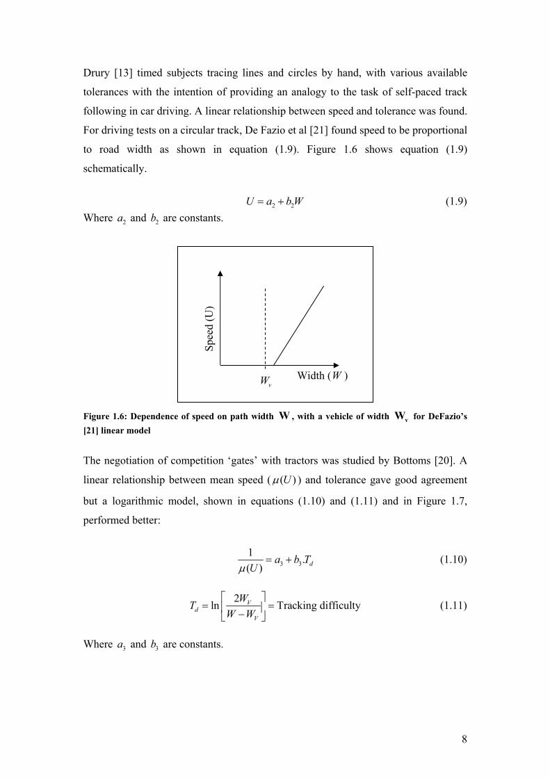
Drury [13] timed subjects tracing lines and circles by hand, with various available
tolerances with the intention of providing an analogy to the task of self-paced track
following in car driving. A linear relationship between speed and tolerance was found.
For driving tests on a circular track, De Fazio et al [21] found speed to be proportional
to road width as shown in equation (1.9). Figure 1.6 shows equation (1.9)
schematically.
2 2U a b W= + (1.9) Where 2a and 2b are constants.
Figure 1.6: Dependence of speed on path width W , with a vehicle of width vW for DeFazio’s [21] linear model
The negotiation of competition ‘gates’ with tractors was studied by Bottoms [20]. A
linear relationship between mean speed ( ( )Uµ ) and tolerance gave good agreement
but a logarithmic model, shown in equations (1.10) and (1.11) and in Figure 1.7,
performed better:
3 31 .( ) da b TUµ
= + (1.10)
2ln Tracking difficultyVd
V
WTW W
= = − (1.11)
Where 3a and 3b are constants.
vW
Spee
d (U
)
Width (W )

9
Figure 1.7: Dependence of speed on path width W with a vehicle of width vW for Bottoms’ [20] logarithmic model
However, as for Drury [13] and De Fazio et al [21], the effect of path curvature is not
included in the model. Bottoms [20] proposed an extension to the model to make it
more suitable for continuous tracking tasks such as road driving. This model included
heading angle tracking difficulty as well as lateral position tracking difficulty, but was
more relevant to very long vehicles such as tractors with trailers, than to cars.
1.2.3 Path error models
Several studies have attempted to characterise speed choice as a function of the
driver’s anticipated path following error [13, 20, 22, 23].
Van Winsum and Gothelp [24] defined a measure of safety margin using the ‘time to
lane crossing’ ( LCT ) which is the predicted time for the vehicle to cross a lane
boundary based on the vehicle’s present trajectory. The driver is assumed to assess the
LCT , and take action to change speed or trajectory to keep LCT above a minimum
acceptable value.
In simulator tests using 40, 80, 120 and 160 m radius curves [24], LCT was found to be
kept above a constant minimum level by drivers. Also, steer angle error was found to
be proportional to steer angle (and hence bend radius). It was claimed that a driver
model with these two features could explain the speed vs. radius behaviour of drivers,
and in turn the reduction of lateral acceleration with speed.
vW Width (W )
Mean Speed ( ( )Uµ )
10
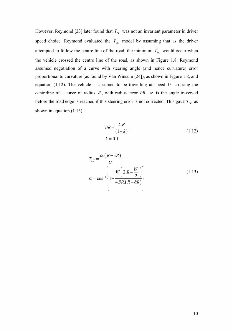
However, Reymond [23] later found that LCT was not an invariant parameter in driver
speed choice. Reymond evaluated the LCT model by assuming that as the driver
attempted to follow the centre line of the road, the minimum LCT would occur when
the vehicle crossed the centre line of the road, as shown in Figure 1.8. Reymond
assumed negotiation of a curve with steering angle (and hence curvature) error
proportional to curvature (as found by Van Winsum [24]), as shown in Figure 1.8, and
equation (1.12). The vehicle is assumed to be travelling at speed U crossing the
centreline of a curve of radius R , with radius error R∂ . α is the angle traversed
before the road edge is reached if this steering error is not corrected. This gave LCT as
shown in equation (1.13).
( ).
10.1
k RRk
k
∂ =+
=
(1.12)
( )
( )1
.
2.2cos 1
4. .
LC
R RT
UWW R
R R R
α
α −
− ∂=
− = − ∂ − ∂
(1.13)
11
Figure 1.8: Reymond's model [23] of Van Winsum’s [24] LCT model, showing the driver steering
with radius error R∂
Reymond evaluated this model for a variety of curve radii, but found that assuming a
constant LCT gave incorrect speed choice behaviour, with little reduction of lateral
acceleration at high speed. This disagreed with the results in the literature [12, 15, 19],
and with Reymond’s own experiments [23].
Reymond [23] instead proposed a lateral acceleration safety margin to explain
reduction of lateral acceleration with speed. This safety margin is predicted by the
driver based on his or her expectation of steering errors, obstacles, or a sudden road
curvature increase. It can therefore be reduced for an expert driver with good
knowledge of the road ahead, but would be increased in the case of an inexperienced
driver following a hazardous road. The safety margin model is shown in equations
(1.14) and (1.15), and illustrated in Figure 1.9.
maxΓ ≤ Γ −∆Γ (1.14) 2
maxC U∆Γ = ∆ (1.15)
Curve radius ( R )
R R−∂ α
Vehicle trajectory with constant steer angle
Curve width (W )
Road edge collision point
12
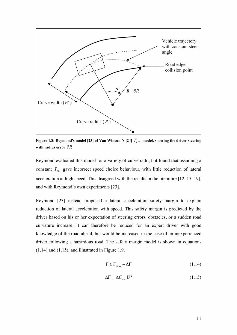
Figure 1.9: Reymond’s [23] lateral acceleration margin model of speed choice
The driver chooses a lateral acceleration Γ that is less than his or her prediction of the
maximum available maxΓ by an amount that is the lateral acceleration safety margin
∆Γ . The margin is proportional to the driver’s uncertainty of the future curvature
deviation maxC∆ , which is independent of speed. In on-road tests it was found that the
curvature margin maxC∆ decreased and maxΓ increased as drivers tried to drive more
urgently. Curvature margin maxC∆ was found to be lower when the same road was
driven on a moving base simulator, and lower still when a fixed-base simulator was
used. maxΓ did not change from road to simulator tests (tyre saturations were included
in the simulator vehicle model).
Reymond’s ‘risk estimation’ bears similarities to an earlier model based on the driver
choosing a speed with acceptable path error proposed by Levison [10]. Levison
proposed the speed choice model as part of the framework for the Interactive
Highway Safety Design Model (IHSDM) which was to be used in the safety
assessment of new highway designs. He did not provide any data to support the model
but proposed it as a starting point for the speed choice module of the IHSDM.
Reymond’s model refers to a curvature deviation, which is directly related to a path
deviation for a given speed. For both models, the safety margin which the driver
allows for this error is assumed to reduce for well known curves, and for confident
drivers. Also, both models were proposed to be based on an assessment of the driver’s
path following error. More recently Cole [22] proposed a more detailed model for
speed choice based on path error. A development of this model is described in chapter
2 section 2.3.
Speed (U ) La
tera
l acc
eler
atio
n (Γ
)
maxΓ Low maxC∆
High maxC∆

13
1.2.4 Coupled models of steering and speed control
Many models of driver steering control also include speed control models in which a
target speed is maintained by closed loop control of the vehicle’s longitudinal
dynamics. The target speed is usually based on the assumption of a maximum lateral
acceleration or a speed limit [25, 26], or a measured speed profile [27].
Prokop [28] provides a more sophisticated speed choice model using a coupled model
of speed control and steering. Prokop’s model plans its path and speed by minimising
a cost function of vehicle state variables: travel time, horizontal accelerations
(longitudinal and lateral), brake use, lane keeping, deviation from desired vehicle
speed and engine speed. Prokop names this strategy ‘Model Predictive Online
Optimisation’ (MPOO). The weightings of the cost function are dependent on the
preferences of the driver, e.g. a driver in a hurry will place high weight on travel time,
and less weight on lateral and longitudinal acceleration. The model then uses a
feedback (compensatory) controller to ensure that the path and speed trajectories
planned by the optimisation process are followed.
The choice of speed is made by the predictive part of the model based on an
assumption that the chosen path will be followed perfectly. No account is taken of
path errors arising from internal or external disturbances, or by imperfect knowledge
of the vehicle dynamics. This would imply that drivers do not assess the accuracy of
their path following control and do not adjust their speed accordingly, which seems to
be an important omission.
1.2.5 Speed adaptation
Speed adaptation is the tendency of drivers to misinterpret their speed after prolonged
exposure to another speed, in the absence of absolute speed information e.g.
speedometer. Since the speedometer is not necessarily used by the driver in speed
judgement for oncoming curves, adaptation could be significant in the speed choice
problem in two ways. Firstly if speed is misperceived this may lead to an improper
selection of an appropriate speed for a particular corner. Secondly if the speed at

14
which a corner was taken was misperceived, this could lead to the incorrect updating
of the driver’s understanding of their own competence e.g. believing that they
managed to go faster or slower than they actually did for a given path error.
Research into the effects of adaptation has been carried out by several researchers
[29-33]. Denton’s experiments [29, 30] aimed to relate the driver’s perceived speed
(U ) to the real vehicle speed (U ). Experiments were carried out in a car [29], and
later in a specially constructed test rig where only visual speed cues were available to
the driver, and where they controlled their speed using a lever [30].
The speed perception errors displayed during Denton’s experiments can be
summarised by Figure 1.10 which shows axes of perceived speed (U ) against actual
speed (U ). It is assumed that the perceived and actual speeds are equal in the fully
adapted (long term) state, because the driver can ‘recalibrate’ their perceived speed
using the speedometer in this long-term case. This fully adapted state is shown as a
dashed line with unity gradient.
Figure 1.10: Adaptation effect on Actual vs. Perceived speed
Two types of test were carried out by Denton, the first in a real car with the
speedometer and engine noise obscured, and the second in a specially constructed test
machine. During the first set of tests subjects asked to double their (perceived) speed
(from 1U to 1ˆ2U ), changed their actual speed by less than a factor of two. This is
Perceived speed (U )
Actual speed (U )
1
2
3
4
Adapted speed
1U 12U
1U
1ˆ2U

15
shown as line (1) in Figure 1.10 which has gradient greater than unity. Drivers asked
to halve their speed reduced their speed by less than a factor of two, shown by line
(3).
The second set of tests were carried out in a test machine where the driver was given
only visual cues of speed by a moving roadway, and had control of the speed of the
roadway using a hand lever. The results of the test are illustrated by Figure 1.10 as
follows:
1. Subjects were adapted to a constant speed ( 1U ) by prolonged exposure to that
speed. The subjects were then suddenly exposed to a higher speed (following
line (1)) causing their perceived speed to be 1ˆ2U .
2. The subjects were then asked to keep their perceived speed ( 1ˆ2U ) constant by
altering their actual speed (U ) using the hand lever. Subjects increased their
actual speed U in order to keep their perceived speed constant (following (2)).
Their speed asymptotically approached the fully adapted speed 12U .
3. The second half of the test was a reversal of the first half. Subjects were
adapted to a higher speed ( 12U ) by prolonged exposure to that speed. The
subjects were then suddenly exposed to a lower speed (following (3)) causing
their perceived speed to become 1U .
4. Subjects were then asked to keep their perceived speed U constant by altering
their actual speed (U ) using the hand lever. Subjects decreased their actual
speed U in order to keep their perceived speed ( 1U ) constant (following (4)).
Their speed U asymptotically approached the fully adapted speed 1U .
The resulting hysteretic behaviour was modelled using a mechanical linear system
analogy as shown in Figure 1.11. Such a model was not suggested by Denton, but fits
to the important aspects of his experimental data. Force ( F ) represents perceived
speed (U ), while position ( x ) represents actual speed (U ). Parameters were fitted to
data from Denton’s experiments [29, 30].

16
Figure 1.11: Mechanical speed adaptation model
First, the unity gradient of the adapted speed line gives:
1 2
1 2
1K KK K
=+
(1.16)
The gradient 1K of the instantaneous speed change lines (1) and (3) was fitted to
Denton’s data [29] giving:
1 1.14K = (1.17) The time constant of the speed change in (2) and (4) is given by:
1
1 2adaptationT
K Kλ
=+
(1.18)
Denton found the time constant to vary with speed from 10 to 25 seconds [30], but is
approximated as 20 seconds for this simulation.
Figure 1.12 shows actual speed recorded during a simulator test, and the resulting
estimated perceived speed from the adaptation model. Having adapted to zero speed
at the start of the test, perceived speed is higher than actual speed. However, after
prolonged exposure to higher speeds, a drop in speed for the last ten seconds causes
perceived speed to be lower than the actual speed.
F
x
1K
2K
1λ

17
5 10 15 20 25 30 35 40 45 50 550
5
10
15
20
25
30Actual speed and Percieved speed due to adaptation
Spe
ed /m
s- 1
Time /s
Actual speedPercieved speed
Figure 1.12: Perceived speed and actual speed for a driver adapted to zero speed at the start of the test
The error in perceived speed is small with the parameter values derived from
Denton’s experiments. The results of Figure 1.12 suggest a maximum 14%
misperception of speed, which only occurs when speed is changed significantly faster
than the 20 second time constant. Denton found the degree of adaptation to be subject
dependent, with some people showing no measurable adaptation tendency.
The effect of including this model of speed adaptation in a path error based speed
choice model was assessed using the speed choice model explained later, in chapter 2
section 2.3. Speed adaptation was found to have little effect on speed choice using the
parameters derived from Denton’s experiments, so the effect of adaptation will not be
included in the discussion of the path error based speed choice model in chapter 2.

18
1.2.6 Summary of speed choice
Table 1.1 shows a summary of the literature on speed choice. Listed are the types of
test performed, models proposed, and the variables measured during experiments.
Ritc
hie,
McC
oy &
Wel
de [1
2]
Dru
ry [1
3]
Her
rin &
Neu
hard
t [15
]
McL
ean
[16]
Bot
tom
s [2
0]
Gaw
ron
& R
anne
y [3
4]
DeF
azio
, Witt
man
& D
rury
[21]
Van
Win
sum
& G
othe
lp [2
4]
Levi
son
[10]
Pro
kop
[28]
Felip
e &
Nav
in [1
9]
Rey
mon
d at
al.
[23]
Col
e [2
2]
1968
1971
1974
1974
1983
1990
1992
1996
1998
1998
1998
2001
2002
non-driving Curve tracing Road driving Track Moving base
Tests simulator driving Fixed-base
Tolerance Radius
Controlled variables/ measurements
Lateral Accel. Lateral Accel. Path error speed
LCT Models
steering MPOO
Table 1.1: Summary of literature on speed choice, where grey indicates inclusion of that test, model or variable
Attempts to characterise speed choice as a function of curvature first concentrated on
lateral acceleration as the major cue. Drivers were observed to reduce their lateral
acceleration as speed increased [12, 14, 15, 19, 23]. Research on the speed of self-
paced tracking tasks as a function of available tolerance successfully fitted models to
the relationship between road width and vehicle speed [13, 20, 21].
Research modelling speed choice as a function of anticipated error, found that a
constant LCT was maintained by the driver, and that steering error increased
19
proportionally with steer angle. However later analysis of this result by Reymond [23]
found that it could not explain drivers’ reduction of lateral acceleration at high speed.
Reymond’s combined model incorporating both lateral acceleration and path error (in
the form of a lateral acceleration margin) was more successful [23]. Drivers’
curvature error margin maxC∆ (equivalent to a path error) was found to change with
driving style, and to decrease in a simulator.

20
1.3 Driver steering control
The development of driver steering control models is well documented, and several
authors have reviewed the field. Guo and Guan [35] provided a comprehensive review
of both compensatory and preview driver models, and Pick [36] and Rutherford [37]
have more recently reviewed the topic. Compensatory and preview controllers are
summarised in the following sections.
1.3.1 Compensatory control
McRuer [38, 39] modelled the performance of a driver in the road path tracking task
using the ‘crossover’ model. In the crossover model, the driver was presumed to use
only visual information of their lateral error to perform feedback lateral position
control. McRuer found that drivers changed their control gains and lead/lag
compensation to ensure good phase margin, and a roll-off of 20dB per decade at the
crossover frequency of the driver-vehicle open loop transfer function. Weir &
McRuer [40] later refined this model to include nested feedback loops for heading
error as well as lateral error. It was found that by using heading angle feedback, no
lead/lag terms were required to stabilise the vehicle, only gain terms. In experiments
McRuer [39] found drivers’ cognitive delay to be approximately 0.2 seconds, and
their actuation delay 0.1 seconds.
Compensatory control models are suitable for modelling the driver’s reaction to
random disturbances such as side-winds. However, drivers also use information
previewed from the road ahead, so preview control models of the driver were
developed to take account of this.
1.3.2 Preview control
McRuer [40] used a single point preview model which eliminated the need for lead
compensation by the driver if the correct look-ahead distance was chosen.
21
MacAdam modelled the driving process using a model predictive preview controller
[41]. This controller compared a target path with a prediction of the vehicle trajectory
assuming present states, and a constant steer angle input. Steer angle input was then
chosen to minimise the error between target and predicted trajectory over the
prediction horizon. Peng [42] noted that this controller is a special case of model
predictive control (MPC). The model was used for the Carsim driver model
(www.carsim.com), and much of the research at the University of Michigan
Transportation Research Institute (UMTRI). Peng [42] extended MacAdam’s use of
predictive control theory to include heading and curvature errors in the cost function
and to allow for non-constant steer angle control.
As mentioned in section 1.2.4, Prokop [28] used a cost function approach, optimising
a more sophisticated cost function than MacAdam [41]. However, this was not model
predictive control (MPC) in its strictest sense, as the planned steering control was
corrected using a compensatory controller, and the optimisation was only used offline
for trajectory planning. Prokop [28] also included a simplified vehicle model for
novice drivers who viewed the vehicle’s transfer function as that of a point mass. This
could be a useful approach when modelling subjects with a range of driving abilities.
Sharp & Valtetsiotis [43] used a linear quadratic regulator (LQR) controller, and
included the previewed road path in the model. This allowed the derivation of a
controller with invariant gains for vehicle states and previewed lateral errors. The
gains were chosen to minimise a cost function of lateral error, heading angle error,
and steer angle input. Choosing the weights of this cost function allows different
control strategies to be chosen. This controller is used extensively in chapters 3, 4 and
5, and its derivation is discussed in detail in chapter 3.
LQR control can be shown to be equivalent to model predictive control (MPC) with
no constraints on controller output or input [44]. The LQR model was shown by
Sharp to give good path following performance while following three different road
paths. Also, Pick [36] developed LQR controllers using a more complex cost function
including lateral acceleration. Pick also incorporated delay into the model by the
addition of delay states.

22
1.3.3 Neuromuscular systems
It may be important when modelling the driver to include the effects of the driver’s
neuromuscular system (NMS). Primarily, the neuromuscular system acts to limit the
bandwidth of the driver’s control because of the limb dynamics and delays inherent in
the system. The neuromuscular system is a limb mass under influence of driver
controlled muscle force, with ‘local’ reflex feedback control to achieve demanded
force or position [36]. The bandwidth limiting properties of the NMS make it an
important element in a driver model.
Magdaleno & McRuer [45] used a 3rd order system to represent the driver’s
neuromuscular system. A simple NMS model was used by MacAdam [46], featuring
pure delay, and a first order low-pass filter. Pick [36] carried out identification of a
limb system transfer function by using a steering wheel shaker test. During this test a
random torque was applied to the steering wheel using an electric motor while the
driver held the steering wheel with both arms. This yielded a second order transfer
function model for the intrinsic (without reflex feedback) limb dynamics as follows:
2
( ) 1( )dem nms nms nms
sT s J s B s Kδ
=+ +
(1.19)
Experiments were conducted with eight subjects with limbs relaxed, and tensed,
giving a range of parameter values for the intrinsic limb natural frequency and
damping. System natural frequency averaged 0.9 Hz with limbs relaxed, and 3.7 Hz
with limbs tensed. Damping ratio averaged 0.43ξ = for relaxed limbs, and 0.24ξ =
for tensed limbs.
Pick also derived a detailed model of the neuromuscular system, and coupled it to an
LQR model to represent the driver. Pick [36] showed that including the driver’s reflex
loop did not alter the transfer function of the limb dynamics dramatically from that of
(1.19), but did cause a slight reduction in system damping.
23
1.3.4 Identification of steering control
Ljung [47] set out principles for identification of systems operating in closed loop in
the presence of noise. Drivers operating in closed loop with a vehicle can only be
identified under specific conditions if mis-identification (called bias) of the identified
parameters is to be avoided [48]. These conditions and Ljung’s system identification
equations are reviewed in detail in chapter 5.
Identification of driver control has been attempted by several authors. McRuer [49]
fitted his crossover model to recorded driver data. MacAdam [41] simulated closed
loop driving using his preview control model and compared the results to those of real
drivers. However, neither of these authors used the system identification methods
described by Ljung to minimise bias.
Recently Rix [48] tested drivers on a fixed-base simulator to identify compensatory
control transfer functions. Rix carried out the experiments in closed loop driving
scenarios designed using the principles set out in Ljung [47]. A side-wind disturbance
was used to excite both the heading error and lateral error control loops, and transfer
functions for both of these loops were derived. Rix only carried out tests for straight
line driving tasks, so a preview controller was not identified. The tests did involve
step changes in the vehicle dynamics, to monitor how drivers adjusted their transfer
function, however, changes in vehicle dynamics arising from speed changes were not
studied.
Pick [36] examined Sharp’s preview model and compared its performance in lane-
change manoeuvres to those found in driver tests. He used trial and error to identify
parameters of the LQR controller to match the driver, but did not use Ljung’s system
identification methods to minimise bias. Also, the driver tests involved repetition of
the same lane-change manoeuvre, so it is possible that the driver could have learnt
open loop steering inputs, rather than rely on preview and compensatory control.
Peng [50] fitted cost function weights of vehicle lateral and heading error for his
model predictive controller to driver data gathered in simulator experiments involving

24
lane changes. However again this did not take account of system identification theory
to minimise the bias of the parameters.

25
1.4 Objectives of research
The findings from the literature review into driver speed and steering control can be
summarised as follows:
At low speed drivers choose their speed to keep below a threshold lateral acceleration
[12]. For high speed driving curvature error (and hence path error) based models like
Reymond’s [23] can predict the reduction of lateral acceleration. However,
measurements of path error from drivers have not been linked to speed choice. Van
Winsum [24] measured steer angle error, and proposed a speed choice mechanism
based on this steering angle error and a constant LCT . However when this model was
tested by Reymond [23], it did not give the correct reduction of lateral acceleration at
high speeds.
An understanding of the driver closed loop steering control is required in order to
model the link between steering angle error and the path error generated by the driver.
Models of compensatory and preview control by drivers are well developed, but few
are well validated. Models of driver preview control have been developed which are
based on minimising a cost function of vehicle and driver performance parameters
[27, 36, 41, 50]. These cost function weights can be varied to change the control
strategy of the driver. Cost function weights have been fitted to measured driver data
for lane-change manoeuvres [36, 50], but only in an ad-hoc way. Bias free estimates
of the controller weights used by drivers have not been published. As a result the
changes in controller weights which could be used to model changes in driver control
strategy with speed or road width are not well validated.
Prokop [28] proposed a driver internal model with simplified vehicle dynamics, and
Peng [50] a model with a simplified cost function, to represent the less sophisticated
preview control of a novice driver. However, these ‘simplified’ preview models have
not been shown to fit data collected from novice drivers better than a preview model
without these simplifications. Neuromuscular systems have been studied, and
included in driver models [36], but have not been incorporated into the driver’s

26
internal model to represent a driver who modifies their control to take account of
knowledge of their own neuromuscular system.
Based on the review of literature on speed choice and steering control, the following
research objectives have been identified:
• To test the link between path error and speed choice by performing simulator
experiments. Experiments should measure driver speed choice and path error
as a function of road geometry, and allow the assessment of a path error based
speed choice model.
• To develop driver models which incorporate the effect of the NMS into the
driver’s internal model to assess the effect of including the driver’s knowledge
of their own bandwidth limitation on their chosen control. Also to incorporate
simplified driver internal models to represent novice drivers.
• To validate models of preview driver steering using simulator data.
Experiments and identification procedures will need to be designed to
minimise identification bias.
• To identify how the steering control of drivers changes with speed and road
geometry in order to quantify how driver steering control influences the
generation of path following error.
Chapter 2 addresses the modelling of speed choice by testing existing models against
simulator data, and assesses a path error based speed choice hypothesis by examining
a subject’s path error and speed choice during a simulator experiment. Chapter 3
describes and compares driver steering models developed from Sharp’s LQR steering
model. These include simplified internal models for novice drivers, and a model of
the neuromuscular system. Chapter 4 describes the design and validation of
identification algorithms and simulator experiments for the identification of driver
preview models from closed loop driver data. Chapter 5 describes the results of this
driver preview model identification from measured simulator data comparing
different driver preview models, test subjects, speeds and road widths. Finally chapter
6 draws conclusions from the work, and suggests directions for future work.

27
Chapter 2: Driver speed choice modelling In this chapter, the existing driver speed choice models reviewed in chapter 1 are
compared using results from simulator experiments carried out at CUED. A path error
based hypothesis for driver speed choice is then proposed and is assessed using path
error and speed choice data measured during the same simulator experiments.
The simulator and experiments are described in section 2.1 and the existing models
are fitted to the simulator data in section 2.2. A new path error based speed choice
model is described in section 2.3, and the path error and speed choice measured
during the simulator experiments is analysed in section 2.4. The results of this
analysis led to the revision of the simulator tests and modelling approach, which is
discussed in section 2.5.

28
2.1 Simulator design and experiments A fixed-base driving simulator was developed for carrying out the speed choice and
steering experiments described in this chapter, and for the experiments described in
chapter 5. This section describes the requirements for the simulator, and how the
CUED simulator was designed to fulfil these requirements. The tests carried out on
driver speed choice using the simulator are then described in section 2.1.7.
2.1.1 Requirements The simulator is a development of the fixed base simulator first set up by Andrew
Pick and Julius Rix at CUED [36, 48]. In order to be used for speed selection
experiments the simulator had to fulfil the following requirements: 1. To avoid simulator sickness, and achieve sufficient fidelity, the time delay for
the visual system should not exceed 40 - 60 ms [51] (see section 2.1.2)
2. The simulator must provide sufficient information for accurate speed
estimation (see section 2.1.3)
3. The driver must be able to select their speed freely, using familiar brake and
accelerator controls (see section 2.1.4).
4. An accurate lateral error constraint must be provided to the driver (see section
2.1.6).
5. The simulator should be able to display the required horizontal road profile,
such as those detailed in section 2.1.7.
Solutions to these requirements are described in the following sections.
2.1.2 Hardware configuration The simulator hardware shown schematically in Figure 2.1 is based around
MATLABTM xPC Target software using a target computer, and a host computer. The
target computer runs the vehicle model using xPC at a cycle rate fast enough to
communicate with the steering wheel hardware at the required 500 Hz. This computer
also runs an A/D card, which reads the pedal position and a D/A card, which outputs

29
two signals for sound generation. The first output signal is a voltage proportional to
speed, which is used to generate a sound with frequency proportional to speed; the
second signal switches on the path constraint buzzer. The host computer performs the
graphics rendering to a projection screen using MATLAB’s virtual reality toolbox.
The required vehicle model is downloaded to the target computer before each test run,
and the recorded variables (position, yaw angle etc.) can be uploaded after the test is
complete.
During the test, some of the variables (position, yaw angle, and speed) are passed to
the host computer at a lower sample rate using a TCP/IP connection. These state
variables are then used to move the driver’s viewing position within a VRML (Virtual
Reality Modelling Language) virtual world which is created before each test to define
the particular path to be driven.
Figure 2.1: Simulator Hardware
VYawYX ,,,
[TCP/IP]
Pedal box
ADC
Steering Wheel
XPC Target Computer
• XPC real time
simulation • Data storage
XPC Host Computer
• VRML World
[CAN bus]
demandTSignal
Generator
DAC
Speaker
Power Amp
Buzzer
[+/- 10V]
Projector
measuredT Angle

30
The simulator was commissioned with three screens giving a 180º visual field as
shown in Figure 2.2. However, with three screens to display, the update rate of the
graphics card was found to be only 20 Hz, and was judged insufficient for use in these
tests. As a result, one screen was used, giving approximately 50 Hz update rate, and a
60º visual field. Using one screen, time delays in the simulator are estimated to
average 20 ms. Approximately ten candidates were tested throughout preliminary and
final testing and of these, two could not be used for prolonged testing due to simulator
sickness. The sickness became apparent within 5 minutes, and worsened to acute
nausea with prolonged testing. None of the five subjects used in final testing (chapter
5) suffered any noticeable simulator sickness.
Figure 2.2: CUED fixed base simulator, showing steering hardware, and three screen display (only the central screen was used during experiments)
2.1.3 Speed perception Three speed cues were provided to the driver. First, a large speedometer on the
simulator screen giving quantitative speed information. Secondly, an audible ‘tone’
whose frequency was proportional to vehicle speed, to imitate the speed dependent

31
road and engine noises of a real vehicle. Thirdly ‘Visual flow’ provides a cue to the
driver, for example, the growth rate of trees as they are approached in the virtual
world.
2.1.4 Vehicle model A two degree of freedom linear bicycle model was used for the yaw and lateral
vehicle dynamics. The bicycle model, as used by many researchers [52-55], is defined
with the parameters shown in Figure 2.3.
Figure 2.3: Bicycle model of vehicle.
The equations of motion are shown in state space form in equation (2.2). The same
formulation is used by Cole [55]. Driver steering wheel angle δ is given by:
f swKδ δ= (2.1) Where swK is the gain between steering wheel angle and front wheel angle.
[ ].
2 2.
f r f r f
sw
ff r f r
sw
C C aC bC CUMU MU MK
aCaC bC a C b CIKIU IU
ν νδ
ωω
+ − − − + = + − + − −
(2.2)
Roll dynamics were not included in the model, so there was no lateral load transfer.
Also, tyre saturations were not included, giving a linear vehicle model. The model
was implemented using MATLAB’s Simulink software, which was then compiled to
fδ ν
ωb U
IM,
a

32
the xPC computer prior to testing. The bicycle model parameters used in testing are
listed in appendix A. For these tests, the vehicle parameters were based on those of a
Vauxhall Vectra as used by Pick [36], but CG position and tyre stiffness were slightly
modified to give a neutral steering vehicle. Steering wheel torque feedback was
proportional to steer angle for all tests.
As well as the lateral-yaw model, a longitudinal model was introduced to allow the
driver to set the vehicle speed using brake and accelerator pedals. Details of the
longitudinal vehicle model are included in appendix B. No interactions between
longitudinal and lateral dynamics were included. The longitudinal model included
influences of engine power, rolling friction, and aerodynamic drag to make the
process of keeping a constant speed as familiar as possible to the driver. The engine
and brake power was set very high (1000 kW) to allow rapid acceleration or
deceleration to a chosen speed. Aerodynamic drag was also high, limiting the vehicle
speed to approximately 65 m/s, but this only had significant effect at high speeds, as
drag force was proportional to 2U .
2.1.5 Road profile construction
Construction of the VRML world through which the subject drove was performed
using a MATLAB function written for this purpose. The function was passed a ‘spine’
vector for the desired road centre line, from which the function created a road whose
left hand lane centre was defined by the spine vector. The road width W refers to the
width of the left hand lane of the road. The road spine equations and widths used for
these tests are discussed in section 2.1.7. Each world included a road, verges, barriers,
and trees of random height, to give visual flow, helping the driver to perceive their
speed.
2.1.6 Lateral error constraint The width of the left hand lane indicated in the visual system provided the lateral
error constraint to the driver. To reinforce this, buzzers sounded whenever the vehicle
left the left hand lane. This occurred when lateral error exceeded ( ) 2vW W− where

33
vW is the vehicle width of 2 metres. In order to activate these buzzers, lateral error
had to be calculated within the xPC target computer.
Lateral error was defined as perpendicular distance from the intended path (road
spine). Lateral error is defined as perpendicular to the path, rather than the vehicle as
this avoids problems when large yaw errors occur.
For the tests described in this chapter, lateral error calculation required an iterative
procedure, which is described in appendix C. This iterative procedure was carried out
‘offline’ i.e. not on the xPC target computer during the testing. To provide a lateral
error constraint during testing, lateral error was pre-calculated for a grid of points on
the x-y plane over which the car drove. This lateral error information was used as a
lookup table to define lateral error as a function of x-y position, and was loaded into
the xPC computer before each test. The xPC computer used this lateral error lookup
table to interpolate a lateral error for the vehicle’s current x-y position, giving a lateral
error accuracy of 0.07m with a 10m lookup table grid resolution.
In the tests described in chapter 5 an algorithm for online lateral error estimation was
developed based on the road spine expressed in intrinsic co-ordinates. This method is
described in appendix D.
2.1.7 Speed choice experiments The simulator experiments whose results are described later in this chapter were
carried out using the fixed-base driving simulator described in the preceding parts of
section 2.1. Each experiment consisted of the test subject driving the vehicle around
twenty-five curves, comprising all permutations of five lane widths (2.4m, 2.8m,
3.2m, 3.6m, and 4.2m), and five radii (66m, 94m, 129m, 190m, and 262m). These
curves were presented in random order so that the driver did not learn the sequence of
speeds necessary. Instead the driver had to choose a speed for each curve based on
their perception of the road ahead.
The road curves consisted of five parts: inward and outward straights, inward and
outward transition sections and a constant curvature section, as shown in Figure 2.4.
Transitions had a linear increase in curvature with distance, giving the curvature
34
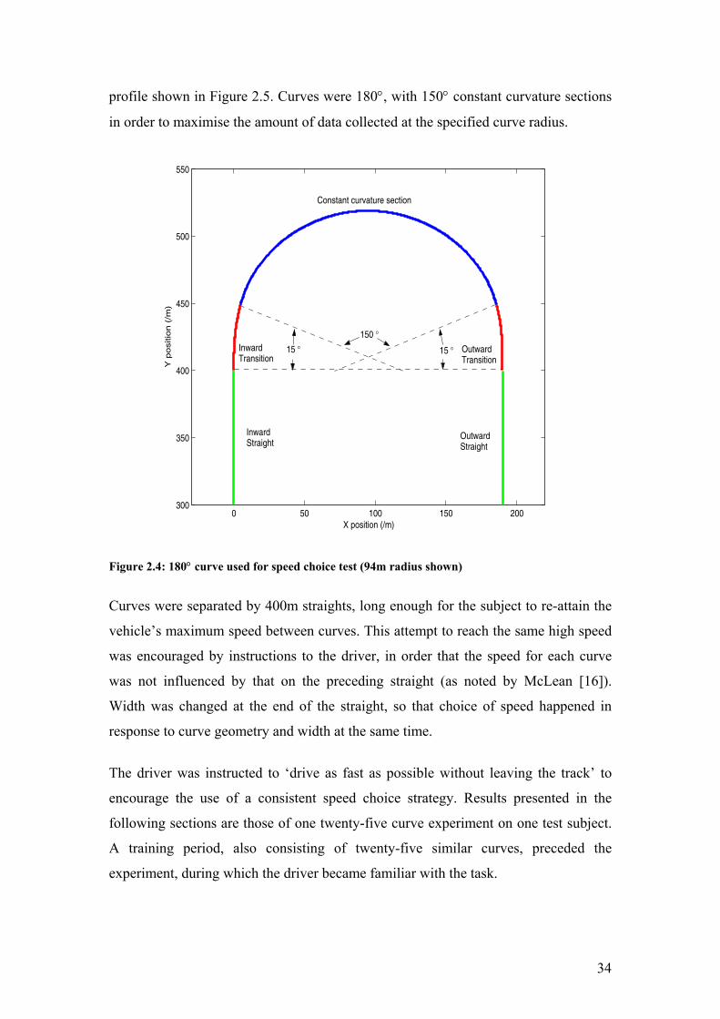
profile shown in Figure 2.5. Curves were 180°, with 150° constant curvature sections
in order to maximise the amount of data collected at the specified curve radius.
0 50 100 150 200300
350
400
450
500
550
X position (/m)
Y p
ositio
n (
/m)
Inward Straight
Outward Straight
Constant curvature section
Inward Transition
Outward Transition
15 °15 °150 °
Figure 2.4: 180° curve used for speed choice test (94m radius shown)
Curves were separated by 400m straights, long enough for the subject to re-attain the
vehicle’s maximum speed between curves. This attempt to reach the same high speed
was encouraged by instructions to the driver, in order that the speed for each curve
was not influenced by that on the preceding straight (as noted by McLean [16]).
Width was changed at the end of the straight, so that choice of speed happened in
response to curve geometry and width at the same time.
The driver was instructed to ‘drive as fast as possible without leaving the track’ to
encourage the use of a consistent speed choice strategy. Results presented in the
following sections are those of one twenty-five curve experiment on one test subject.
A training period, also consisting of twenty-five similar curves, preceded the
experiment, during which the driver became familiar with the task.

35
The data shown in this chapter are from a single test subject, so limited conclusions
can be drawn about the speed choice of a population of drivers. However, the data
allows comparison of the existing models, and examination of the speed choice trends
present in the simulator experiment. Also, the single driver’s data is able to illustrate
important trends in the path error and speed choice of drivers which led to the revision
of the modelling approach, and a change of experimental technique for the remaining
chapters of the thesis. Other data were collected with this subject and other subjects
that were consistent with the findings shown in this chapter for the single test subject.

36
2.2 Data analysis A typical measured speed profile is shown in Figure 2.5. On first entering the curve,
an ‘open loop’ speed is achieved, and is the driver’s choice of speed based on preview
of the approaching curve. The driver then modifies this speed once in the constant
curvature section to a (sometimes lower) ‘closed loop’ speed.
2600 2800 3000 3200 3400 3600 3800 400020
40
60
Spe
ed U
(/m
s−1 )
Curve Centerline Distance /m
2600 2800 3000 3200 3400 3600 3800 40000
0.005
0.01
Speed
Curvature
’Open loop’ Speed
’Closed loop’ Speed
Cur
vatu
re C
(/m
−1)
Figure 2.5: Speed and curvature profile for a typical curve
The open loop speed may be different from the closed loop speed for several reasons:
• The driver may have poor speed control of the vehicle, so the driver’s
intended speed on entry to the constant curvature section is not attained.
• The speed chosen for a transition may be intentional, but different from the
constant curvature speed due to the presence of changing curvature, or the
uncertainty of the final bend curvature.
• The driver may not be familiar with the simulated vehicle’s lack of lateral
acceleration limit, so may be able to increase their speed beyond their initial
estimate. However, this effect should be eliminated by the training period.
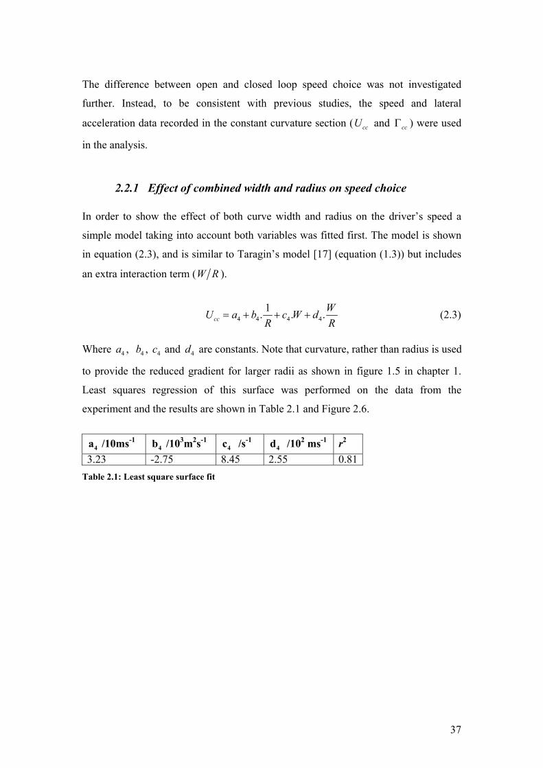
37
The difference between open and closed loop speed choice was not investigated
further. Instead, to be consistent with previous studies, the speed and lateral
acceleration data recorded in the constant curvature section ( ccU and ccΓ ) were used
in the analysis.
2.2.1 Effect of combined width and radius on speed choice In order to show the effect of both curve width and radius on the driver’s speed a
simple model taking into account both variables was fitted first. The model is shown
in equation (2.3), and is similar to Taragin’s model [17] (equation (1.3)) but includes
an extra interaction term (W R ).
4 4 4 41. . .cc
WU a b c W dR R
= + + + (2.3)
Where 4a , 4b , 4c and 4d are constants. Note that curvature, rather than radius is used
to provide the reduced gradient for larger radii as shown in figure 1.5 in chapter 1.
Least squares regression of this surface was performed on the data from the
experiment and the results are shown in Table 2.1 and Figure 2.6.
4a /10ms-1 4b /103m2s-1 4c /s-1 4d /102 ms-1 r2
3.23 -2.75 8.45 2.55 0.81Table 2.1: Least square surface fit

38
24
68
1012
1416
x 10−3
2
2.5
3
3.5
4
4.510
20
30
40
50
60
70
Curvature C (/m−1)Width W (/m)
Spe
ed U
cc (
/ms−
1 )
Figure 2.6: Speed ccU vs. curvature C vs. width W
Fit is good ( 2 0.81r = ), showing increasing speed with increasing width and
decreasing curvature. There is not much surface warping, suggesting that the
interaction term in (2.3) could be omitted. Fitting this surface without the interaction
term gave similarly good fit ( 2 0.80r = ). This implies that the dependence of speed on
width was similar irrespective of the curvature.
2.2.2 Effect of lateral acceleration on speed choice
Reymond’s lateral acceleration margin model [23] (equations (1.14) and (1.15)) was
fitted to the measured data. Results for the narrowest (2.4m) and widest (4.2m) curves
are shown in Figure 2.7 and Figure 2.8. The data points show measured ccΓ vs. ccU .
For comparison, radius contours for 66m and 262m are also shown as dashed lines.
An envelope of maximum lateral acceleration at each speed (as used by Reymond) is
shown as a solid line, and a least squares fit of the Reymond model to this envelope is
shown as a dotted line. The fitted values of the model parameters and the correlation
coefficient are shown in Table 2.2 for each curve width.
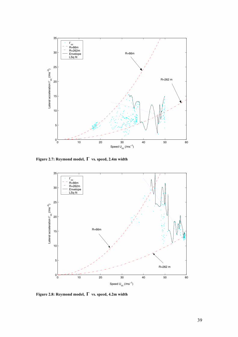
39
0 10 20 30 40 50 600
5
10
15
20
25
30
35
Speed Ucc
(/ms−1)
Late
ral a
ccel
erat
ion Γ cc
(/m
s−2 )
Γcc
R=66mR=262mEnvelopeLSq fit
R=262 m
R=66m
Figure 2.7: Reymond model, Γ vs. speed, 2.4m width
0 10 20 30 40 50 600
5
10
15
20
25
30
35
Speed Ucc
(/ms−1)
Late
ral a
ccel
erat
ion Γ cc
(/m
s−2 )
Γcc
R=66mR=262mEnvelopeLSq fit
R=66m
R=262 m
Figure 2.8: Reymond model, Γ vs. speed, 4.2m width

40
The correlation coefficients are low except for the widest road, so the model
coefficients derived for the narrowest four roads are not reliable. However, the widest
three roads do show a clear drop-off in lateral acceleration with speed similar to that
in Figure 2.8. The maximum lateral acceleration parameter maxΓ is much larger than
the -210 ms recorded by Reymond, presumably because there is no tyre saturation in
the simulator vehicle model, and no lateral acceleration cue to the driver. Also the
maximum lateral acceleration ( maxΓ ) is seen to increase appreciably for the wider
roads. The curvature margin maxC∆ is of similar magnitude to that of Reymond, who
found max 3.82C∆ = km-1 with a standard deviation of 0.77km-1 for his static simulator
tests. This demonstrates that lateral acceleration reduced with speed even though there
was no tyre saturation.
Width /m 2.4 2.8 3.2 3.6 4.2 maxΓ /m s-2 14.6 9.61 23.9 24.2 51.5
max∆C / (km)-1 2.88 -1.83 3.09 2.48 11.5 r2 0.09 0.05 0.13 0.08 0.65
Table 2.2: Reymond lateral acceleration model
2.2.3 Effect of curve radius on speed choice The LCT criterion [24] suggests a direct relationship between speed choice and curve
radius [23]. Reymond’s lateral acceleration margin model can also be rearranged to
give such a relationship (eqn (2.4)). In this section, these two models are fitted to the
mean speed ( ( )ccUµ ) and curve radius ( R ) data. An envelope function such as that
shown Figures 2 and 3 is not used.
2.2.3.1 Reymond lateral acceleration margin model Recorded mean speed and radius for each of the twenty-five curves is shown in Figure
2.9, along with a least squares fit of equation (2.4) for each curve width.
max2
max max
1 1 1( )cc
CU Rµ
∆ = + Γ Γ (2.4)

41
0 50 100 150 200 250 3000
10
20
30
40
50
60
Radius R (/m)
Spe
ed U
cc (
/ms−
1 )
W=4.2 mW=3.6 mW=3.2 mW=2.8 mW=2.4 m
W=4.2 W=3.6
W=3.2
W=2.8
W=2.4
Figure 2.9: Reymond model, speed vs. radius, widths 2.4 to 4.2m
The correlation coefficients (Table 2.3) are much better than those in Table 1, largely
because the mean speed ( )ccUµ has been used, rather than the maximum lateral
acceleration envelope. Also the effect of radius on speed is clearer on these axes.
maxC∆ and maxΓ are similar in magnitude to those of section 2.2.2, and again both
increase with increasing curve width. It is clear that curve width affects speed
significantly, although curve width is not included in this lateral acceleration based
model.
The least squares fitted line for the 2.4m width road in Figure 2.9 does not seem to fit
the points well, despite having 2 0.81r = . The reason for the apparently poor fit is that
the regression was performed to minimise the least squares error of 21 U , rather than
U . The fitted line has increasing gradient at large radii in contrast to all of the other
widths, and a trend which is not apparent in the data. This gives rise to negative
curvature margin maxC∆ , which would imply increased lateral acceleration with
increased speed.

42
Width / m 2.4 2.8 3.2 3.6 4.2
maxΓ /m s-2 4.47 16.0 28.9 25.1 38.6
max∆C /(km)-1 -2.57 2.50 6.33 3.45 7.24r2 0.81 0.64 0.49 0.91 0.95
Table 2.3: Reymond speed vs. radius model
2.2.3.2 Time to lane crossing model Reymond’s model [23] of Van Winsum’s constant LCT hypothesis [24] (equation
(1.13)) leads to the following:
( ) [ ]71( ) . .1cc
LC
U a RT k
µ α= ++
(2.5)
For this model, and all models in section 2.2.4, the mean speed ( )ccUµ for each curve
is used. Figure 2.10 shows the resulting fit of equation (2.5).
0 50 100 150 200 250 3000
10
20
30
40
50
60
Radius R (/m)
Spe
ed U
cc (
/ms−
1 )
W=4.2 mW=3.6 mW=3.2 mW=2.8 mW=2.4 m
W=3.6
W=3.2
W=2.8
W=2.4
W=4.2
Figure 2.10: LCT model, speed vs. radius, widths 2.4 to 4.2m
The fitted lines are curved because α is a function of radius. The velocity offset value
7a was not present in Reymond’s model [23], but is necessary to allow a regression
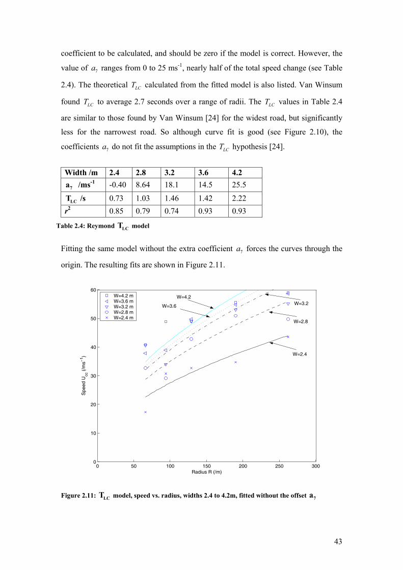
43
coefficient to be calculated, and should be zero if the model is correct. However, the
value of 7a ranges from 0 to 25 ms-1, nearly half of the total speed change (see Table
2.4). The theoretical LCT calculated from the fitted model is also listed. Van Winsum
found LCT to average 2.7 seconds over a range of radii. The LCT values in Table 2.4
are similar to those found by Van Winsum [24] for the widest road, but significantly
less for the narrowest road. So although curve fit is good (see Figure 2.10), the
coefficients 7a do not fit the assumptions in the LCT hypothesis [24].
Width /m 2.4 2.8 3.2 3.6 4.2
7a /ms-1 -0.40 8.64 18.1 14.5 25.5
LCT /s 0.73 1.03 1.46 1.42 2.22 r2 0.85 0.79 0.74 0.93 0.93
Table 2.4: Reymond LCT model
Fitting the same model without the extra coefficient 7a forces the curves through the
origin. The resulting fits are shown in Figure 2.11.
0 50 100 150 200 250 3000
10
20
30
40
50
60
Radius R (/m)
Spe
ed U
cc (
/ms−
1 )
W=4.2 mW=3.6 mW=3.2 mW=2.8 mW=2.4 m
W=4.2 W=3.2
W=2.8
W=2.4
W=3.6
Figure 2.11: LCT model, speed vs. radius, widths 2.4 to 4.2m, fitted without the offset 7a

44
Eliminating the coefficient 7a leads to an undefined 2r value in the regression, so
goodness of fit cannot be quantified. However, Figure 2.11 reveals a qualitatively
poorer agreement with the data, especially for the wider roads. Also, if 7 0a = had
given a better fit, it would have been chosen in the previous regression. The LCT
values derived are listed in Table 2.5. The values are more consistent than those of
Table 2.4, but are significantly less than those found by Van Winsum [24].
Width /m 2.4 2.8 3.2 3.6 4.2
LCT /s 0.74 0.83 0.91 1.00 1.13
Table 2.5: Reymond LCT model
2.2.4 Effect of curve width on speed shoice
2.2.4.1 De Fazio et al linear model De Fazio et al’s linear model [21] of speed vs. width (equation (1.9)) is fitted to each
radius separately in Figure 2.12.
2.4 2.6 2.8 3 3.2 3.4 3.6 3.8 4 4.2 4.40
10
20
30
40
50
60
Width W (/m)
Spe
ed U
cc (
/ms−
1 )
R=262 mR=190 mR=129 mR=94 mR=66 m
R=262
R=190
R=129
R=94
R=66
Figure 2.12: Linear model speed vs. width, radii 66 m to 262 m

45
Fitted coefficients 2a and 2b are shown in Table 2.6. Fit is not as good as that
observed by De Fazio [21], with 2r from 0.66 to 0.89. Close examination suggests
that a curve would fit the points better than this straight line, such that less increase in
speed is seen at higher widths.
Radius /m 66 94 129 190 262
2a /ms-1 -3.12 1.58 17.0 17.7 24.9 2b /s-1 11.4 10.7 8.54 9.91 8.75
r2 0.66 0.89 0.69 0.65 0.87 Table 2.6: De Fazio et al linear model
2.2.4.2 Tracking difficulty model Fitting of the measured data to Bottoms’ tracking difficulty model [20] (equations
(1.10) and (1.11)), is shown in Figure 2.13.
2.4 2.6 2.8 3 3.2 3.4 3.6 3.8 4 4.2 4.40
10
20
30
40
50
60
Width W (/m)
Spe
ed U
cc (
/ms−
1 )
R=262 mR=190 mR=129 mR=94 mR=66 m
R=262 R=190
R=129
R=94
R=66
Figure 2.13: Bottoms’ model, speed vs. width, radii 66 m to 262 m
Unlike De Fazio et al’s linear model, the curves show the appropriate reduction of
gradient at high speed, and a corresponding improvement in 2r (Table 2.7). The curve

46
with 66m radius does not seem to fit the data well, but the regression of this model
minimises 1 U , rather than U . Tracking difficulty dT was much lower than that
recorded by Bottoms since the road is much wider relative to the vehicle than in his
experiments with tractors. However, the model’s intended mechanism based on driver
limited cognitive capacity still applies since the instructions were to go as fast as the
driver was capable.
Radius /m 66 94 129 190 262
3a /10-2m-1s 0.75 1.90 1.47 1.25 1.41
3b /10-2m-1s 1.90 0.71 0.62 0.62 0.38r2 0.80 0.72 0.86 0.80 0.97
Table 2.7: Bottoms’ tracking difficulty model
2.2.4.3 Time to lane crossing model Reymond’s LCT model from section 2.2.3.2 can be fitted to the data to predict the
dependence of speed on road width, because the angle α is a function of road width.
Reymond’s derivation of the LCT model assumed that road edge collision occurred
when the vehicle’s CG crossed the road edge i.e. when lateral error reached 2W .
However, in testing, the road edge constraint (when the buzzers sounded) was for
lateral error exceeding ( ) 2vW W− i.e. when the edge of the vehicle crossed the road
edge. The available width ( )vW W− was therefore used in equation (1.13) in place of
W . The available width ( )vW W− was also used in section 2.2.3.2 to calculate angle
α . Figure 2.14 shows the fit of Reymond’s LCT model to the measured data. Again
the velocity offset 7a was included to allow a regression coefficient to be calculated.
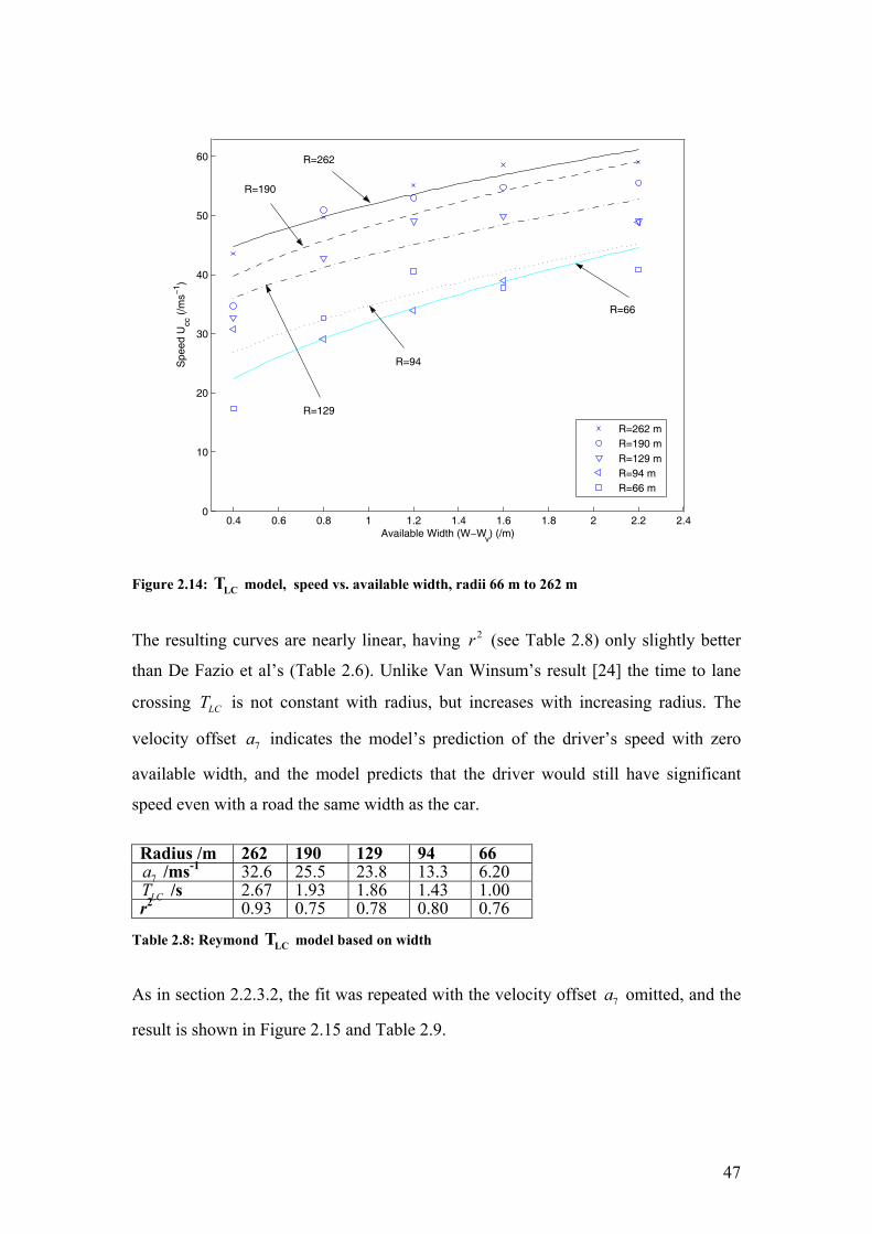
47
0.4 0.6 0.8 1 1.2 1.4 1.6 1.8 2 2.2 2.40
10
20
30
40
50
60
Available Width (W−Wv) (/m)
Spe
ed U
cc (
/ms−
1 )
R=262
R=66
R=94
R=129
R=190
R=262 mR=190 mR=129 mR=94 mR=66 m
Figure 2.14: LCT model, speed vs. available width, radii 66 m to 262 m
The resulting curves are nearly linear, having 2r (see Table 2.8) only slightly better
than De Fazio et al’s (Table 2.6). Unlike Van Winsum’s result [24] the time to lane
crossing LCT is not constant with radius, but increases with increasing radius. The
velocity offset 7a indicates the model’s prediction of the driver’s speed with zero
available width, and the model predicts that the driver would still have significant
speed even with a road the same width as the car.
Radius /m 262 190 129 94 66
7a /ms-1 32.6 25.5 23.8 13.3 6.20 LCT /s 2.67 1.93 1.86 1.43 1.00
r2 0.93 0.75 0.78 0.80 0.76
Table 2.8: Reymond LCT model based on width
As in section 2.2.3.2, the fit was repeated with the velocity offset 7a omitted, and the
result is shown in Figure 2.15 and Table 2.9.
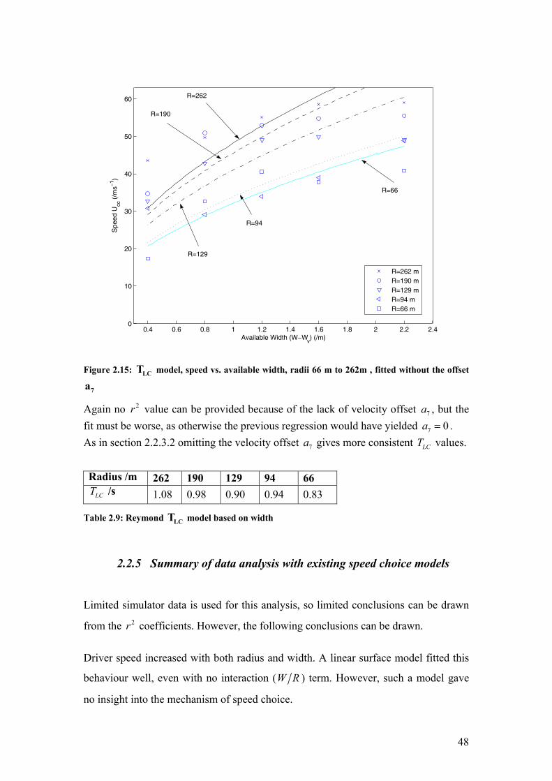
48
0.4 0.6 0.8 1 1.2 1.4 1.6 1.8 2 2.2 2.40
10
20
30
40
50
60
Available Width (W−Wv) (/m)
Spe
ed U
cc (
/ms−
1 )
R=262
R=190
R=129
R=94
R=66
R=262 mR=190 mR=129 mR=94 mR=66 m
Figure 2.15: LCT model, speed vs. available width, radii 66 m to 262m , fitted without the offset
7a
Again no 2r value can be provided because of the lack of velocity offset 7a , but the fit must be worse, as otherwise the previous regression would have yielded 7 0a = . As in section 2.2.3.2 omitting the velocity offset 7a gives more consistent LCT values.
Radius /m 262 190 129 94 66
LCT /s 1.08 0.98 0.90 0.94 0.83
Table 2.9: Reymond LCT model based on width
2.2.5 Summary of data analysis with existing speed choice models Limited simulator data is used for this analysis, so limited conclusions can be drawn
from the 2r coefficients. However, the following conclusions can be drawn.
Driver speed increased with both radius and width. A linear surface model fitted this
behaviour well, even with no interaction (W R ) term. However, such a model gave
no insight into the mechanism of speed choice.
49
The driver data showed a reduction of lateral acceleration at high speed for widest
three roads despite the vehicle model including no tyre saturations. This lends weight
to a curvature error or path error based explanation for the reduction in lateral
acceleration such as Reymond’s lateral acceleration margin model.
Mean speed increased with increasing radius such that reduced gradient occurred at
larger radii. Reymond’s lateral acceleration margin model was able to predict this
behaviour well for most widths, but did not take account of the curve width. Speed
increased with width such that a reduced gradient of speed vs. width was seen for
wide roads. De Fazio’s linear model could not provide the required reduction in
gradient at large widths. Bottoms’ model was able to provide this reduction in
gradient giving improved fit, but was unable to model radius dependence.
Reymond’s LCT model was able to predict both the radius and width dependence of
speed with similarly good fit to other models. However, the speed offset 7a was
significantly greater than the zero that was predicted by Van Winsum. Omission of 7a
gave poorer fit, but more consistent LCT . Good fit of this model was therefore not
achieved with the assumptions of Van Winsum’s original model.
From this analysis, none of the models could provide all three requirements of:
o Good fit
o A mechanistic model whose assumptions were met by the fitted parameters
o An ability to predict both width and radius dependence.
A new model of speed choice should incorporate the successful features from the
existing models. Firstly, lateral acceleration dependence should be included, as it
conveniently models the driver’s low speed behaviour found in real driving
experiments in the presence of lateral acceleration and tyre saturations [12]. Secondly,
the use of anticipated driver error (such as curvature error or path error) is the most
promising mechanistic model of driver speed choice. A model which could include
this feature and also predict the influence of path width (unlike Reymond’s model)
would be desirable.

50
2.3 Speed choice model hypothesis
A hypothesis (Figure 2.16) is proposed in this section based on speed choice as a
function of both lateral acceleration [10, 12, 15, 16, 23, 34], and path error [10, 13,
16, 20, 22, 34] as follows:
(1) Upon approach to a corner, its curvature is assessed by the driver, and an
estimate of the path error allowable on the corner is made.
(2) Previous experience allows the driver to anticipate lateral acceleration and
path error on the corner for a given speed. Experience is stored in the form of
lookup tables of speed vs. path error, and speed vs. lateral acceleration
(3) The driver decides on what speed to negotiate the corner by minimising a cost
function based on travel time through the corner, lateral acceleration, and path
error. The weights of the three components are dependent on the motivation of
the driver.
(4) After negotiating the corner, the driver uses the actual lateral acceleration and
path error achieved for that curve to update their experience.
Though lateral acceleration is important to the speed choice of drivers its influence is
reasonably well understood. This work concentrated on identifying the part of the
speed choice decision arising from path error estimation, rather than from lateral
acceleration effects. This enabled the use of a fixed base driving simulator, and linear
tyre models. The effects of path error on speed choice could then be studied in the
absence of lateral acceleration cues and limits, and without the more complex changes
in vehicle handling brought about by tyre saturations (e.g. understeer to oversteer
transitions at high lateral acceleration).

51
Figure 2.16: Speed selection hypothesis overview
Sources of path error are proposed as follows:
(1) External sources e.g. side winds, road roughness.
(2) Internal Driver sources
a) Imperfect feedforward control, from incomplete learning of the vehicle
dynamics.
b) Driver measurement and actuation noise e.g. Perception of path, motor
control.
c) Intentional driver (open loop) inputs.
No external noise sources were provided to the driver during testing, so external noise
sources (1) were not present. This work concentrated on the driver internal noise
sources a) and b), and assumed that intentional (open loop) inputs by the driver were
not present. An empirical model for path error prediction by the driver is proposed as
follows.
Set weights 1W , 2W , 3W
1 95 0 2 31( )pJ W y W WU
ρ= + Γ +
Select U to minimise J
Path Error
( 95 0( )pyρ )
Lateral Acceleration (Γ )
Speed (U )
(1) (2) (3) Speed (U )
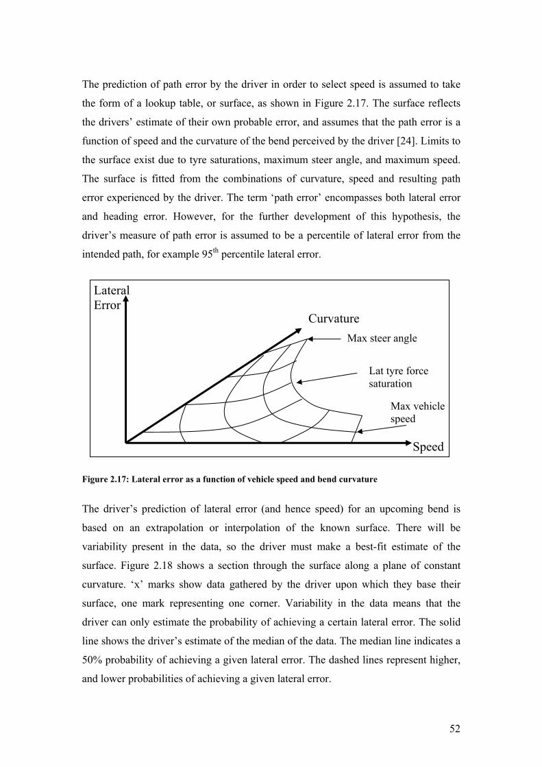
52
The prediction of path error by the driver in order to select speed is assumed to take
the form of a lookup table, or surface, as shown in Figure 2.17. The surface reflects
the drivers’ estimate of their own probable error, and assumes that the path error is a
function of speed and the curvature of the bend perceived by the driver [24]. Limits to
the surface exist due to tyre saturations, maximum steer angle, and maximum speed.
The surface is fitted from the combinations of curvature, speed and resulting path
error experienced by the driver. The term ‘path error’ encompasses both lateral error
and heading error. However, for the further development of this hypothesis, the
driver’s measure of path error is assumed to be a percentile of lateral error from the
intended path, for example 95th percentile lateral error.
Figure 2.17: Lateral error as a function of vehicle speed and bend curvature
The driver’s prediction of lateral error (and hence speed) for an upcoming bend is
based on an extrapolation or interpolation of the known surface. There will be
variability present in the data, so the driver must make a best-fit estimate of the
surface. Figure 2.18 shows a section through the surface along a plane of constant
curvature. ‘x’ marks show data gathered by the driver upon which they base their
surface, one mark representing one corner. Variability in the data means that the
driver can only estimate the probability of achieving a certain lateral error. The solid
line shows the driver’s estimate of the median of the data. The median line indicates a
50% probability of achieving a given lateral error. The dashed lines represent higher,
and lower probabilities of achieving a given lateral error.
Speed
Lateral Error
CurvatureMax steer angle
Lat tyre force saturation
Max vehicle speed
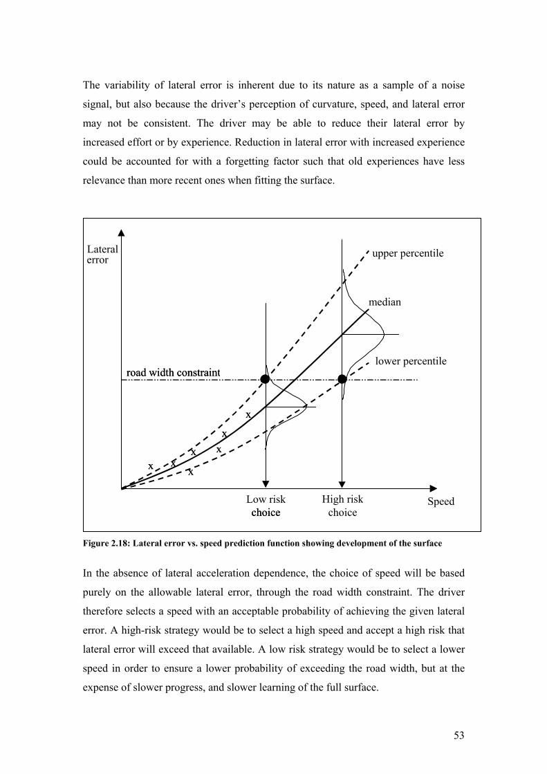
53
The variability of lateral error is inherent due to its nature as a sample of a noise
signal, but also because the driver’s perception of curvature, speed, and lateral error
may not be consistent. The driver may be able to reduce their lateral error by
increased effort or by experience. Reduction in lateral error with increased experience
could be accounted for with a forgetting factor such that old experiences have less
relevance than more recent ones when fitting the surface.
Figure 2.18: Lateral error vs. speed prediction function showing development of the surface
In the absence of lateral acceleration dependence, the choice of speed will be based
purely on the allowable lateral error, through the road width constraint. The driver
therefore selects a speed with an acceptable probability of achieving the given lateral
error. A high-risk strategy would be to select a high speed and accept a high risk that
lateral error will exceed that available. A low risk strategy would be to select a lower
speed in order to ensure a lower probability of exceeding the road width, but at the
expense of slower progress, and slower learning of the full surface.
Speed
Lateral
x x
x
x x
x
x
upper percentile
lower percentile
High riskchoice
Low riskchoice
road width constraint
error
x x
x
x x
x
x
choice
road width constraint
median

54
Data from the simulator tests described in section 2.1.7 were used test this hypothesis,
the results are presented in the next section. During tests instructions were given to try
and keep the risk strategy constant, so it was assumed that the driver would have a
consistent risk strategy independent of road width.

55
2.4 Data analysis for path error model
The speed choice hypothesis presented in the previous section (2.3) relies on
establishing the dependence of the driver’s lateral error on speed, radius and width.
This lateral error dependence is therefore investigated in sections 2.4.1 to 2.4.6.
Limited data from only one subject are used to illustrate the dependence of lateral
error on speed, so it is not possible to validate the hypothesis based on these results. A
single driver’s data is shown as it is able to illustrate important features of the
dependence of the driver’s lateral error on road width, without the complexity of
comparison between subjects. More importantly, the results of one subject are able to
illustrate the need for a revision of the modelling approach, and a change of
experimental technique. This change of approach meant that only a limited number of
subjects were tested using this method. However, other data from this subject and
from the two other subjects tested was consistent with the results shown in this
section.
The new modelling approach was required in order to identify the steering behaviour
of the test subjects. The results of this section show that an ability to quantify the
driver’s steering behaviour is an important part of a speed choice model. The
identification of driver steering behaviour is the subject of the remaining chapters of
the thesis.
2.4.1 Lateral error vs. time histograms Figure 2.19 shows histograms of the lateral error vs. number of samples (at 500 Hz)
for the constant curvature part of the curve, for each of the 25 curves in the test. The
curves are sorted by width and radius, with the largest radius, widest road at the lower
right of the figure, and the smallest radius, narrowest road on the upper left. 95th
percentile lateral error ( 95 0( )pyρ ) is shown on each plot as a dashed red line.

56
Figure 2.19: Lateral error histogram for each curve
The distribution of lateral error for most of the curves is non-normal, and the peaks
caused by individual excursions from the centre line are visible in the histograms.
Finding the 95th percentile lateral error 95 0( )pyρ (or other percentiles) of these
distributions is therefore an inaccurate representation of the true statistics of the data.
Ideally, more data would be gathered for each radius and width to provide a normal
distribution for each radius and width combination. However, in the absence of this
data another approach was taken, in which several curves were grouped together by
either radius or width. This approach is shown in sections 2.4.3 and 2.4.4. The
disadvantage of grouping data by width or radius is that some variable interactions are
not visible, so first the lateral error vs. speed vs. curvature surface proposed in the
hypothesis was fitted to the ‘ungrouped’ curve data as shown in section 2.4.2.
0
100
200no
. of s
ampl
es(R
= 6
6 m
)
W=2.4 m W=2.8 m W=3.2 m W=3.6 m W=4.2 m
0
100
200
no. o
f sam
ples
(R=
94
m)
0
100
200
no. o
f sam
ples
(R=
129
m)
0
100
200
no. o
f sam
ples
(R=
190
m)
−1 0 10
100
200
no. o
f sam
ples
(R=
262
m)
yp0
(/m)−1 0 1
yp0
(/m)−1 0 1
yp0
(/m)−1 0 1
yp0
(/m)−1 0 1
yp0
(/m)

57
2.4.2 Lateral error vs. speed vs. curvature
Although the histograms of section 2.4.1 showed 95th percentile lateral error 95 0( )pyρ
for individual curves to be unreliable, it is useful to plot a surface of the form given in
equation (2.6) to illustrate the interactions of the three variables. The surface relates a
percentile (λ ) of lateral error ( 0( )pyλρ ) to the mean speed in the constant curvature
part of the curve ( ( )ccUµ ), and curve curvature (1 R ) including an interaction term
( ( )ccU Rµ ).
0 5 5 5 5( )1( ) ( ) cc
p ccUy a b c U d
R Rλ λ λ λ
λµρ µ= + + + (2.6)
Where 5a λ , 5b λ , 5c λ and 5d λ are constants for a particular lateral error percentile λ .
Figure 2.20 shows the 95th percentile lateral error ( 95λ = ) surface from equation
(2.6) fitted to the data from the simulator experiment.
24
68
1012
1416
x 10−3
10
20
30
40
50
60
−0.5
0
0.5
1
1.5
Speed µ(Ucc
) (/ms−1)
Curvature C (m−1)
ρ 95(y
p0)
Figure 2.20: 95 p0ρ (y ) vs. curvature C vs. speed ccµ(U ) , with surface fitted from equation (2.6)

58
The regression coefficient for the surface ( 2 0.44r = ) was poor but this was to be
expected given the non-normal distribution of the lateral error for each curve.
The dependence of speed on curvature demonstrated in Figure 2.6 has led to the
driver only using a part of the surface in the lateral error vs. speed vs. radius axes.
There are therefore no points for low curvature at low speed, or high curvature at high
speed. In order to fully populate this surface, an experiment with speed as a controlled
variable would be required.
2.4.3 Lateral error vs. curvature Figure 2.21 shows the same lateral error data as the histograms of Figure 2.19
grouped by curve radius. Again 95 0( )pyρ for each radius is shown as a dashed red
line. Each group contains data from all five widths, so any dependence on width will
not be visible in these plots.
−2 0 20
500
1000
1500
2000R = 262 m
no. o
f sam
ples
−2 0 2
R = 190 m
−2 0 2
R = 129 m
yp0
(/m)
−2 0 20
500
1000
1500
2000R = 94 m
no. o
f sam
ples
yp0
(/m)−2 0 2
R = 66 m
yp0
(/m)
Figure 2.21: Histograms of lateral error ( p0y ) samples at 500 Hz, grouped by radius. Red
dashed line shows 95 p0ρ (y )

59
Grouped by radius, the data is more like a normal distribution, so percentiles of these
histograms become more meaningful. The smaller radius bends take less time, so have
less data, giving a less normal distribution. 95th percentile lateral error ( 95 0( )pyρ )
from Figure 2.21 is plotted against curve curvature in Figure 2.22.
Figure 2.22: Lateral error 95 p0ρ (y ) vs. curvature C
Figure 2.22 shows that lateral error 95 0( )pyρ is nearly independent of curvature.
Speed ( )ccUµ is dependent on curvature (see Figure 2.6) therefore Figure 2.22
supports the hypothesis of the driver attempting to keep 95 0( )pyρ constant by
changing speed.
If Figure 2.20 is viewed along the direction of the speed axis the same independence
of lateral error and curvature can be seen.
0 0.002 0.004 0.006 0.008 0.01 0.012 0.014 0.0160
0.2
0.4
0.6
0.8
1
Curvature /m−1
ρ 95(Y
p0)
(/m
)
ρ
95(Y
p0)
Linear least squares fit

60
2.4.4 Lateral error vs. width Figure 2.23 shows the same lateral error data as Figure 2.19 grouped by curve width.
Again 95 0( )pyρ for each width is shown as a dashed red line.
−2 0 20
500
1000
1500
2000W=2.4 m
no. o
f sam
ples
−2 0 2
W=2.8 m
−2 0 2
W=3.2 m
yp0
(/m)
−2 0 20
500
1000
1500
2000W=3.6 m
no. o
f sam
ples
yp0
(/m)−2 0 2
W=4.2 m
yp0
(/m)
Figure 2.23: Histograms of p0y samples at 500 Hz, grouped by width. Red dashed line shows
95 p0ρ (y )
Distributions are again nearly normal, but with distortions still visible in the tails of
the distributions due to individual excursions from the road centre. Figure 2.24 shows
95th percentile lateral error 95 0( )pyρ from Figure 2.23 plotted against the ‘available
tolerance’ ( ) 2vW W− . The solid black line indicates lateral error equal to available
tolerance ( 0( ) ( ) 2p vy W Wρ = − ).

61
Figure 2.24: Lateral error 95 p0ρ (y ) vs. available tolerance ( v(W - W ) 2 ) for radii 66m to 262m
The assumption of the hypothesis of section 2.3 was that lateral error would match the
available tolerance as a result of the driver adjusting his speed to use the whole road
width. As a result, the driver would aim for the same lateral error percentile for all
widths.
The results of Figure 2.24 support the hypothesis that lateral error is altered to take
advantage of road width. However, Figure 2.24 shows that 95 0( )pyρ exceeds the
available tolerance for narrow roads, but is less than the available tolerance for wide
roads.
This implies that the driver is not changing his speed enough to make
95 02. ( ) ( )p vy W Wρ − independent of W . Two possible reasons have been identified
for this behaviour:
0 0.2 0.4 0.6 0.8 1 1.20
0.2
0.4
0.6
0.8
1
Available tolerance (W−Wv)/2 (/m)
ρ 95(Y
p0)
(/m
)
ρ
95(Y
p0)
Linear least squares fit
62
1. It may be a risk strategy inherited from road driving, given that accidents more
severe at high speed.
2. The driver may change their steering control strategy in response to width. It
would then be possible for the driver to achieve different lateral error for the
same radius and speed by using different steering control strategies (requiring
different amounts of control effort).
Changes in driver control strategy (or effort) would require a different version of the
lateral error vs. speed curve in Figure 2.18 for each level of driver effort. In order to
quantify the steering strategy parameter, it is necessary to look more closely at the
driver’s steering control to quantify how it changes with speed, width, or between
drivers. This is the subject of the work in chapters 3, 4 and 5, and is discussed in
section 2.5.
The path error hypothesis can be modified to take account of the ‘risk’ part of the
behaviour observed in Figure 2.24, so that the driver aims to achieve a different lateral
error percentile (λ ) for each width. This modification is examined in section 2.4.6.
2.4.5 Lateral error vs. speed It is not as easy to plot lateral error as a function of speed, because speed was not a
controlled variable of the experiment. The data from the constant curvature section of
the curves was therefore grouped in speed bands of 10m/s width, and histograms of
these bands are shown in Figure 2.25.

63
0
1000
2000
3000
4000
15<Ucc≤25
no. o
f sam
ples
25<Ucc≤35
−2 0 2
35<Ucc≤45
yp0
(/m)
−2 0 20
1000
2000
3000
4000
45<Ucc≤55
yp0
(/m)
no. o
f sam
ples
−2 0 2
55<Ucc≤65
yp0
(/m)
Figure 2.25: Histograms of p0y samples at 500 Hz, grouped by ccU . Red shows 95 p0ρ (y )
There are different amounts of data in each speed band, and as a result, the poorly
populated distributions are not as normal as those for grouping by width or radius.
95th percentile lateral error 95 0( )pyρ was plotted against the speed at the centre of
each speed band in Figure 2.26.
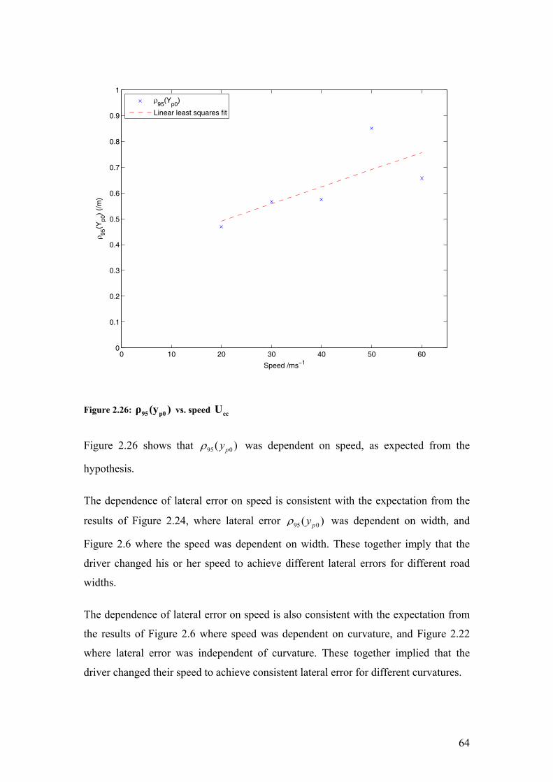
64
Figure 2.26: 95 p0ρ (y ) vs. speed ccU
Figure 2.26 shows that 95 0( )pyρ was dependent on speed, as expected from the
hypothesis.
The dependence of lateral error on speed is consistent with the expectation from the
results of Figure 2.24, where lateral error 95 0( )pyρ was dependent on width, and
Figure 2.6 where the speed was dependent on width. These together imply that the
driver changed his or her speed to achieve different lateral errors for different road
widths.
The dependence of lateral error on speed is also consistent with the expectation from
the results of Figure 2.6 where speed was dependent on curvature, and Figure 2.22
where lateral error was independent of curvature. These together implied that the
driver changed their speed to achieve consistent lateral error for different curvatures.
0 10 20 30 40 50 600
0.1
0.2
0.3
0.4
0.5
0.6
0.7
0.8
0.9
1
Speed /ms−1
ρ 95(Y
p0)
(/m
)
ρ
95(Y
p0)
Linear least squares fit

65
2.4.6 Speed prediction using hypothesis
The hypothesis of section 2.3 can be modified to take account of the risk/effort
behaviour observed in section 2.4.4 by assuming that the driver aimed to achieve a
different lateral error percentile (λ ) for each width. The fitting of this modified
‘variable risk’ hypothesis is described in the sections 2.4.6.1 to 2.4.6.3.
In order to fit this modified hypothesis it must be assumed that the driver effort is
constant, and that the driver’s risk behaviour accounts for the change in lateral error
percentile λ with width. The reasons for this are described in section 2.4.6.2.
Although constant effort was encouraged by instructions to the driver, the possibility
that the driver effort was not constant cannot be discounted. This modified ‘variable
risk’ speed choice hypothesis can therefore not be considered a complete solution to
the problem identified in section 2.4.4, as driver effort must be quantified. Defining
the driver effort through modelling of driver steering control is the subject of the work
in chapters 3, 4 and 5.
The ‘variable risk’ path error based speed choice hypothesis was fitted to the driver
data, and its prediction of speed was compared with the linear surface model shown in
section 2.2.1. The model of section 2.2.1 was chosen for comparison as this predicts
the influence of both radius and width. Speed prediction using the ‘variable risk’ path
error hypothesis involved the following steps.
1. Establish the lateral error percentile Wλ chosen for each width (risk behaviour).
2. Fit a lateral error ( 0( )pyλρ ) vs. speed vs. curvature surface for each
percentile Wλ .
3. Predicted speed can then be determined from the fitted surface.
2.4.6.1 Lateral error percentile vs. width First, the lateral error percentile λ chosen for each width was established as discussed
in section 2.4.4 . This was carried out using an optimisation routine in MATLAB to
solve equation (2.7) for each width 1W to 5W .

66
1
10 1
( )arg min ( ( ))2
vW p
W W y Wλ λλ ρ − = −
(2.7)
Where 0 1( ( ))py Wλρ is the λ th percentile of the lateral error recorded for width 1W in
the constant curvature section (shown in Figure 2.23). This yields five percentiles 1Wλ
to 5Wλ . The five percentiles 1Wλ to 5Wλ are plotted against the widths 1W to 5W in
Figure 2.27.
0 0.2 0.4 0.6 0.8 1 1.240
50
60
70
80
90
100
Available tolerance (W−Wv)/2 (/m)
Per
cent
ile o
f pat
h er
ror λ
Figure 2.27: Percentile (λ ) of p0y vs. available tolerance ( )vW - W 2
The result is consistent with that of Figure 2.24, and shows that the subject was within
the road for 55% of the time on the narrowest road, but 96% of the time on the widest
road.
2.4.6.2 Lateral error surface fitting Next, for each of the widths, a lateral error vs. speed vs. curvature surface must be
fitted using equation (2.6) as demonstrated in section 2.4.2. For example, for width
1W the surface for the 55th percentile lateral error ( 0( )pyλρ where 1 0.55Wλ λ= = ),

67
yielding four surface coefficients 1 1 1 15 5 5 5[ , , , ]W W W Wa b c d . This procedure is repeated for
each of the percentiles 1Wλ to 5Wλ to establish four surface coefficients for each of the
widths 1W to 5W .
This is can be thought of as plotting contours of λ for the three dimensional field
0( ){ , , }py C Uρ λ . Fitting of a λ surface to this field uses all the data, rather than just
that for the width corresponding toλ . This presumes that the field 0( ){ , , }py C Uρ λ is
independent of width.
However, this may not be the case if driver control strategy is being changed between
widths. It would then be possible for the driver to achieve different lateral error
0( ){ }pyρ λ for the same curvature and speed { , }C U point by using different control
strategies. It would then be necessary to define a 4th dimension to the field, to take
account of this control strategy (or effort) parameter Θ , giving a field
0( ){ , , , }py C Uρ λ Θ . A constant effort Θ was assumed for this model. However, to
better understand the driver speed choice, a means of defining this driver effort
parameter Θ will be important. Defining the driver steering strategy (or effort)
through modelling of driver steering control is the subject of the work in chapters 3, 4
and 5 and is discussed in section 2.5.
2.4.6.3 Speed prediction Predicted speed ( 'ccU ) for each curve can then be determined from the surface
corresponding to the correct width for that curve. For example, for width 1W , the
surface coefficients 1 1 1 15 5 5 5[ , , , ]W W W Wa b c d are used in equation (2.8) (a rearrangement of
(2.6)) to yield the predicted speed for the five curves of width 1W .
( )
11
1
11
51 5
55
(( ) / 2 )'
WW
vW
cc WW
bW W aRU
dcR
− − −=
+ (2.8)
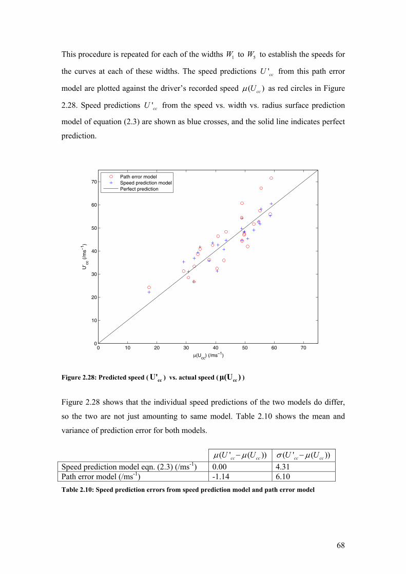
68
This procedure is repeated for each of the widths 1W to 5W to establish the speeds for
the curves at each of these widths. The speed predictions 'ccU from this path error
model are plotted against the driver’s recorded speed ( )ccUµ as red circles in Figure
2.28. Speed predictions 'ccU from the speed vs. width vs. radius surface prediction
model of equation (2.3) are shown as blue crosses, and the solid line indicates perfect
prediction.
0 10 20 30 40 50 60 700
10
20
30
40
50
60
70
µ(Ucc
) (/ms−1)
U′ cc
(/m
s−1 )
Path error modelSpeed prediction modelPerfect prediction
Figure 2.28: Predicted speed ( ccU' ) vs. actual speed ( ccµ(U ) )
Figure 2.28 shows that the individual speed predictions of the two models do differ,
so the two are not just amounting to same model. Table 2.10 shows the mean and
variance of prediction error for both models.
( ' ( ))cc ccU Uµ µ− ( ' ( ))cc ccU Uσ µ− Speed prediction model eqn. (2.3) (/ms-1) 0.00 4.31 Path error model (/ms-1) -1.14 6.10 Table 2.10: Speed prediction errors from speed prediction model and path error model

69
The speed prediction model has zero mean prediction error because the surface was
fitted to ensure that the mean error of the residuals is zero. The mean prediction error
for the path error model is low considering the non-normal data used to populate the
0( ){ , , }py C Uρ λ field.
The path error model is significantly more complicated than the speed prediction
model, and gave no benefit in prediction accuracy. The assumption of constant driver
effort necessary to fit this model also renders it less useful. To validate this model
properly, different data should be used for fitting the model to that used for evaluating
the model. Instead of collecting this data, it was preferred to spend time on a new set
of experiments, designed to resolve the issue of changing driver effort.

70
2.5 Discussion
The experiments described in this chapter were not designed to enable the driver’s
steering control strategy (or effort level) to be quantified. In order to enable the
driver’s steering strategy to be determined, the fitting (identification) of a driver
steering model with an appropriate ‘effort’ parameter to driver steering data was
required. An identified steering model would allow the variation of steering control
(or effort) with speed and track width to be quantified.
Sharp’s LQR preview model allows driver steering strategy to be modelled using cost
function weights on lateral error and heading error, so was chosen as a suitable driver
model. The development of driver models based on Sharp’s LQR controller is
described in chapter 3.
A revised set of experiments were undertaken in order to quantify the changes in the
driver steering strategy with speed and road width. A range of fixed speeds and road
widths was used so that the variation of driver performance (including path error) and
steering control (effort) could be measured as a function of speed and road width. A
group of five subjects was used in order to quantify the variation in steering strategy
between drivers.
In order to identify the preview driver model without bias, notice had to be taken of
the system identification theory set out by Ljung [47]. A suitable experimental design
using a random road input to excite the driver’s preview control had to be validated.
The validation of this method is described in chapter 4, and the results of the driver
identification are described in chapter 5.
71
2.6 Conclusions The conclusions for the existing speed choice models were covered in the summary in
section 2.2.5, leading to the proposal of the new path error based speed choice
hypothesis. Conclusions from assessment of the path error based speed choice
hypothesis using measured simulator data are as follows:
Lateral error histograms for individual curves were non-normal, so fitting percentiles
to these provided poor statistics. Data was therefore ‘lumped’ together to examine
lateral error as a function of width, radius, and speed separately. This led to more
normal distributions. Lateral error was independent of bend curvature, but speed was
not, indicating that speed and/or steering control was changed in order to keep lateral
error constant. Lateral error changed with width, but not by enough to keep the ratio
of lateral error to available tolerance constant. The cause of non-constant lateral error
to available tolerance ratio could be a risk strategy, or a change in steering control
strategy (effort) by the driver. Although only one test subject’s results are shown here,
data from earlier tests showed similar trends.
A variable percentile of lateral error with width was added to the path error based
speed choice model to take account of this behaviour, but it was necessary to assume
constant driver effort. The prediction of speed using this modified ‘variable risk’
hypothesis gave poorer fit than the linear speed vs. width vs. curvature surface model
of equation (2.3), despite the path error model’s increased complexity. Although the
limited data does not enable the speed choice model to be validated, the results
illustrate the importance of the relationship between path error and speed in the
modelling of speed choice.
It was concluded that changes in driver steering control (effort) could affect the speed
choice of drivers. Because of this possibility new experiments were proposed to
examine the changes in the steering control of drivers with speed and road width. The
experiments proposed involved driving random roads at a range of fixed speeds, and

72
road widths. The driver steering strategy was to be determined by fitting preview
steering control models to the measured steering control action of the driver.

73
Chapter 3: Models of driver steering control
Chapters 3 to 5 deal with the possibility of modelling the driver’s steering control as a
linear quadratic regulator (LQR). This chapter introduces a set of candidate LQR
models with varying degrees of sophistication, while chapter 4 introduces and
validates identification procedures for fitting these models to measured data. The
results of fitting the LQR models to driver data are then presented in chapter 5.
This chapter is split into four sections. Firstly, the LQR controller concept and the
way it is implemented is explained. Secondly, a set of LQR models with varying
degrees of sophistication is proposed. Thirdly, the preview and state gains of these
controllers are investigated, including how they change with speed. Finally closed
loop control with each controller is implemented and the performance of the
controllers is compared.
A set of LQR models with varying degrees of sophistication was required for two
reasons. Firstly it was unclear at this stage how sophisticated a model was required to
reflect a ‘typical’ human driver. A model set with a range of complexities was used to
find out the minimum complexity required to fit the ‘typical’ driver’s behaviour
closely. Secondly there may be significant variability between drivers due to different
levels of competence at steering. Steering competence may be affected by experience,
natural ability, or attentiveness of the driver. A range of driver models was required to
ensure that each driver can be matched closely enough by one of the models of the
set.
Ideally an infinitely large model set would be used, but this work was limited to LQR
models. LQR models were chosen as they incorporate many of the important features
known to be present in control by real drivers, but are simple to implement as they
have linear time invariant gains.

74
3.1 Introduction to Sharp’s LQR controller
Sharp proposed an LQR controller with road preview as a model of the driver for
moderate steering manoeuvres [43]. In this section the derivation of Sharp’s model is
explained and modifications are proposed to make the model more representative of
real driver behaviour.
3.1.1 The LQR controller
The derivation of the LQR controller involves a vehicle model coupled to a road
model via a cost function. This cost function is chosen to reflect the priorities of the
driver in terms of path following, heading error minimisation, or steer angle
minimisation. Derivation of the controller begins with a description of the bicycle
model of the vehicle (Figure 2.3) in state space form:
Figure 3.1: Bicycle model of vehicle
f swKδ δ= (3.1) Where δ is the driver’s steering wheel angle, and swK is the gain between steering
wheel angle and front wheel angle.
δ= +v vx Ax B (3.2)
fδ ν
ωb U
IM,
a

75
For a 2DOF bicycle model this takes the form [55]:
[ ]Tvyν ω θ=vx (3.3)
11 12 1
21 22 2
0 00 0
and 1 0 0 00 1 0 0 0
A A BA A B
U
= =
A B (3.4)
111 122 2
21 22 2
and
f r f r f
sw
ff r f r
sw
C C aC bC CUMU MU MKBA A
A A B aCaC bC a C b CIKIU IU
+ − − − + = = − + − −
(3.5)
Secondly, the road is described in ground-fixed axes ( ),x y in terms of offsets riy
from the x -axis shown in Figure 3.2.
Figure 3.2: Road and preview offsets in ground-fixed ( )x, y axes
UT UT
UT
0ry 2ry 3ry rhy…
x
y
θ
ν
U x
y
vy 1ry

76
The road is modelled in discrete state space form such that each timestep T a new
road point rhy is introduced at the end of the vector of preview offsets ry and the
remaining points move down the vector ry by means of a shift register:
( 1) ( ) rhk k y+ = +r ry Dy E (3.6)
0 1 0 0 00 0 1 0 0
and 0 0 0 1 00 0 0 0 1
= =
D E (3.7)
Discretising A and B from equation (3.4) using MATLAB function C2D gives dA
and dB . The vehicle and road discrete state space models can then be amalgamated:
( 1) ( )0 0
0( 1) ( ) 0rh
k ky
k kδ
+ = + + +
v v dd
r r
x x BAD Ey y
(3.8)
The two models are not linked in (3.8), but are linked by the introduction of a cost
function. The cost function proposed by Sharp is as follows:
1 20
lim { ( ). . ( ) ( ). . ( )}n T
nk
J k k k kδ δ→∞=∑= +z R z R (3.9)
Where:
[ ]0 1T
v r r rhy y y yν ω θ
= =
v
r
xz
y (3.10)
The parameter 2R sets the driver’s cost on steer angle, while the matrix 1R sets the
driver’s cost on combinations of states. In Sharp’s formulation, the cost on steer angle
( 2R ) is kept constant:
1=2R (3.11)

77
The vehicle states cost matrix 1R is then varied (relative to 2R ) to set the driver’s
preferences. In Sharp’s formulation, the state cost matrix 1R is formulated as follows:
1 1T=1R C QC (3.12)
1
0 0 1 0 1 0 0 0 01 10 0 0 1 0 0 0
UT UT
− = −
C (3.13)
0
0yq
qθ
=
Q (3.14)
The parameters yq and qθ set driver’s cost of lateral error and heading error
respectively. The driver can therefore vary their costs on lateral error ( yq ) and
heading error ( qθ ) independently to set his or her driving strategy preference. The
MATLAB function DLQR is then used to calculate an LQR controller from equations
(3.8), (3.12) and (3.13), yielding a controller of the type:
0
h
y v ri rii
k k k y k k yν ω θδ ν ω θ=∑= = + + + +LQRK z (3.15)
This controller can then be reformulated in terms of preview offsets piy measured in
the driver reference frame (offsets measured from the driver’s ‘optical lever’ as shown
in Figure 3.3), as detailed by Sharp and later Cole [43, 55]. In this vehicle reference
frame, equation (3.15) simplifies to equation (3.16) (for the 2DOF bicycle model
above):
0
h
pi pii
k k k yν ωδ ν ω=∑= + + (3.16)

78
Figure 3.3: Preview offsets measured in vehicle reference frame ( )x, y
The resulting controller uses the same preview gains ( =pi rik k ) and vehicle state
gains ( , )k kν ω , but the gains yk and kθ become zero and can be removed from the
controller. The elimination of ( ),yk kθ was found by Cole [55] to be conditional on
the preview being sufficiently long for the preview gains to decay to zero at the
furthest point ( 0phk = ). Care needs to be taken therefore when selecting preview
length for controllers.
3.1.2 Proposed modifications to LQR controller
Sharp’s LQR controller [43] provides most of the features necessary in a good driver
model, namely: preview of the future road path; feedback of present vehicle states; an
internal model of the system to be controlled; and parameters to specify the control
priorities (effort level) of the driver. However, certain limitations of Sharp’s model
were identified which could be remedied with modifications to the LQR formulation.
Each of these modifications was incorporated into one or more models of the set to
provide greater or sophistication than Sharp’s model. The limitations, and the
modifications made to Sharp’s formulation are as follows.
0py 1py
2py 3py phy
x
y
θ
ν
U
UT UT
UT
y
x
vy

79
Firstly, the LQR controller presumes perfect knowledge of the vehicle by the driver.
This may not be the case for novice drivers, who might assume a simplified vehicle
model and be able to use this to control the vehicle in relatively benign situations (i.e.
low sideslip and yaw acceleration conditions). This means of modelling a novice
driver was used by Prokop [28]. Two LQR controllers based on simplified vehicle
models are described in sections 3.2.2 and 3.2.3.
Secondly the controller assumes infinite bandwidth of driver control, whereas in fact
the driver’s control is band-limited. The use of a second order filter to approximate
the neuromuscular system (NMS) models proposed by Pick [36] was discussed in
chapter 1. A second order filter NMS model is incorporated into the LQR formulation
in sections 3.2.5 and 3.2.6.
Finally, the driver is subject to significant time delay between measurement of vehicle
states and actual steer angle application. These delays occur during perception,
decision making and actuation of the neuromuscular system and are thought to total
between 0.15 and 0.3 seconds [36, 39, 41]. These delays are not represented in the
LQR formulation as explained so far. An LQR formulation taking account of delay
was proposed by Pick [36] and this model is detailed in section 3.2.4.
A limitation that could not be remedied with modifications to Sharp’s model was the
restriction of linear time invariant (LTI) control inherent in the LQR controller. A real
driver is not restricted to LTI control, and may act non-linearly in the presence of
constraints such as road edges. A model predictive controller could provide this
feature, but requires a different modelling approach than that used here for the LQR
controller. Study of model predictive controllers may be carried out in future work,
but was not attempted as part of this thesis. Instead, an LQR controller must model
the presence of a more restrictive road edge constraint by using a higher controller
weighting on lateral and/or heading error. There may be other limitations of LQR
controllers, so one objective of this work was to see how well the LQR controller fits
to driver data.
80
3.2 Description of Models
A range of LQR models was necessary to cover all of the possible modifications
above. In this section eight models are proposed. All models are intended to control
the same vehicle (second order bicycle model in equation (3.4)), but each model
represents a different level of control sophistication of the driver.
Model IG is that proposed by Sharp [43] as detailed in section 3.1. Models IIG and
IIIG are of reduced complexity compared to the plant being controlled, to represent
the simplified controller of a novice driver. The concept of a reduced complexity
model for novice drivers was as proposed by Prokop [28], who used a point mass
vehicle model. Model IVG includes the inherent driver delay as formulated by Pick
[36]. Models VG to VIIIG include a neuromuscular system (NMS) model. In three of
these models ( VIG to VIIIG ) the driver is aware of the neuromuscular system and
changes their LQR control to compensate, whereas in model VG the driver is not
aware of its presence and uses a controller optimised with no NMS. The eight models
and their equations are described in sections 3.2.1 to 3.2.6.
3.2.1 Model IG : Second order bicycle model
Model IG is the LQR controller detailed by Sharp [43] and in section 3.1. The model
represents an experienced driver with full knowledge of the yaw and sideslip
behaviour of the vehicle.

81
Figure 3.4: State and preview inputs and output of model IG
The resulting controller shown in Figure 3.4 requires preview, but also both yaw and
sideslip ( ),ν ω states of the vehicle. This model is parameterised by the two weights
{ },yq qθ on lateral error and heading error respectively.
3.2.2 Model IIG : Zero order model
Model IIG is a simplified version of the real vehicle system intended to characterise a
novice driver with a simplified internal model of vehicle. This vehicle is modelled as
a point-mass, as shown in Figure 3.6 and behaves according to equation (3.18) from
Prokop [28]. Figure 3.5 and equation (3.17) show the derivation of equation (3.18) .
Figure 3.5: Derivation of Prokop’s point mass model
fδ
fδ
a
b
( )tan( )f
a bδ+
R
Driver Model IG
LQR controller
{ },yq qθLQRK(1: )p hy
νω
δ
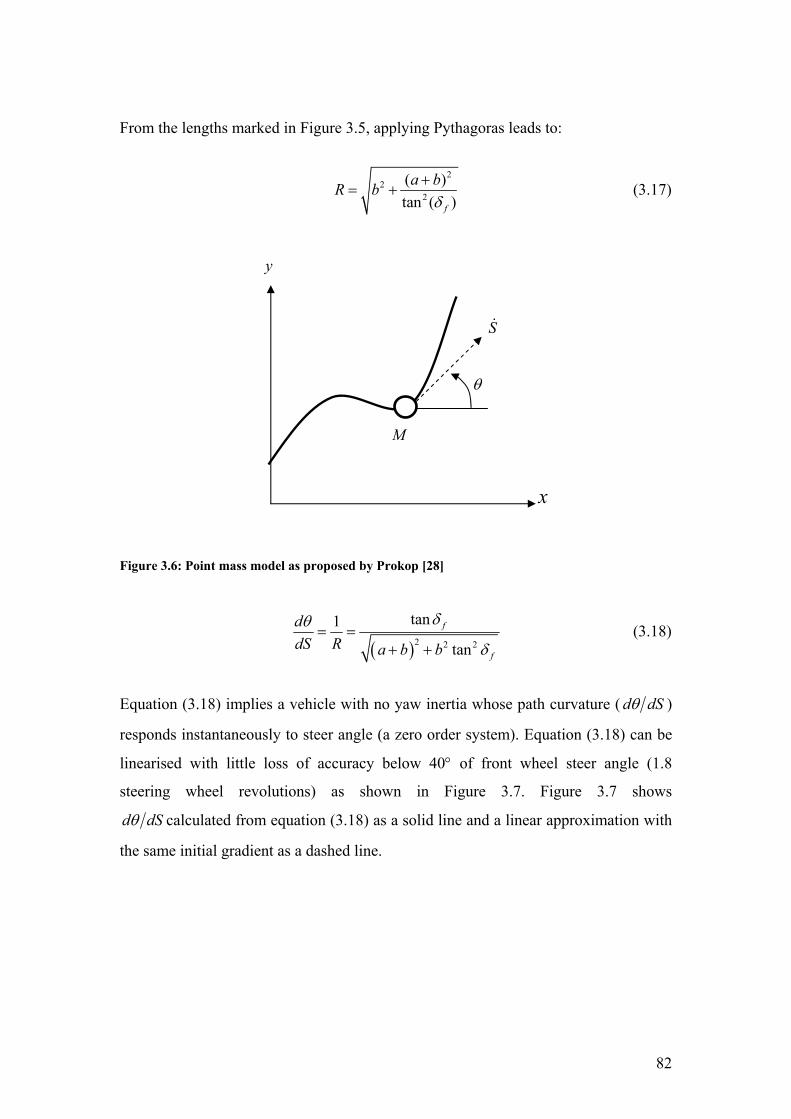
82
From the lengths marked in Figure 3.5, applying Pythagoras leads to:
2
22
( )tan ( )f
a bR bδ
+= + (3.17)
Figure 3.6: Point mass model as proposed by Prokop [28]
( )2 2 2
tan1
tan
f
f
ddS R a b b
δθ
δ= =
+ + (3.18)
Equation (3.18) implies a vehicle with no yaw inertia whose path curvature ( d dSθ )
responds instantaneously to steer angle (a zero order system). Equation (3.18) can be
linearised with little loss of accuracy below 40° of front wheel steer angle (1.8
steering wheel revolutions) as shown in Figure 3.7. Figure 3.7 shows
d dSθ calculated from equation (3.18) as a solid line and a linear approximation with
the same initial gradient as a dashed line.
θ
S
x
M
y

83
0 10 20 30 40 50 600
0.02
0.04
0.06
0.08
0.1
0.12
0.14
Front wheel steer angle δf (/°)
Pat
h cu
rvat
ure
dθ/d
S (
m−
1 )
Prokop point mass modelLinear at initial gradient
Figure 3.7: Front wheel steer angle fδ vs. path curvature dθ dS in Prokop’s point mass model
Linearising equation (3.18) gives yaw rate as shown in equation (3.19):
( )12 2 2
tantan
f
f
d d dS S kdt dS dt a b b
θ θω δ δδ
= = = ≈+ + (3.19)
If yaw rate gain 1k is chosen to be consistent with the 2DOF system of equation (3.4),
then the system equation (analogous to that of equation (3.2)) is:
2
22
000 0
y U yBA
δθθ
= +
(3.20)
The resulting LQR controller derived from equations (3.8) to (3.15) and (3.20) is
shown schematically in Figure 3.8.

84
Figure 3.8: State and Preview inputs and output of LQR controller for model IIG
The resulting model ( IG ) has no vehicle state inputs, only path preview, so the novice
driver being modelled takes no account of the vehicle’s present velocity states in his
or her control. Model parameters are { },yq qθ as for Sharp’s controller ( IG ).
3.2.3 Model IIIG : 1DOF model
As for model IIG , IIIG is a simplified vehicle model intended to mimic a novice
driver, but of slightly more sophistication. Model IIIG is based on the 2 DOF bicycle
model of equation (3.4), but with the sideslip (ν ) degree of freedom removed. Zero
sideslip can be achieved with various rear wheel steering strategies [52], which are
not under the control of the driver, therefore ensure that drivers do not need to take
account of sideslip in their control of the vehicle. Sideslip is small in most normal
driving situations, so model IIIG might be used by a normal driver with little
experience of tyre saturation conditions.
The system equation for model IIIG is shown in equation (3.21). Steady state yaw rate
gain is the same as that of equation (3.4) (model IG ).
222 0 0
0 0 01 0 0 0
BAy U yω ω
δθθ
= +
(3.21)
Figure 3.9 shows the driver model controller for model IIIG :
Driver Model IIG
LQR Controller
{ },yq qθLQRK(1: )p hy δ

85
Figure 3.9: State and preview inputs and output of model IIIG
The ‘model IIIG ’ driver requires both preview and vehicle yaw rate (ω ) state
information to decide on steer angle, but not sideslip velocity (ν ). Again the model is
parameterised by two controller weights { },yq qθ .
3.2.4 Model IVG : Delay state model
Model IVG was proposed by Pick [36] as a means of including the driver’s knowledge
of his or her own cognitive and actuation delay (τ ) in the driver’s internal model. The
model includes extra ‘delay states’ for delay of steer angle into the vehicle. This
allows modelling of a driver who is aware of his or her own delay and changes their
control accordingly.
The state space equations to be used in the LQR controller are shown in discrete form
in equation (3.22). Input steer angle dNδ is delayed by its passage down a shift
register before it is applied to the vehicle. The number of delay states ( dN )
corresponds to number of time steps of delay.
Driver Model IIIG
LQR controller
{ },yq qθLQRK(1: )p hy
ω δ

86
1
2
1
1 11 12
2 21 22
3
4
( 1) 0 0 0 0 0 0 0 0( 1) 1 0 0 0 0 0 0 0
( 1) 0 0 0 0 0 0 0 0( 1) 0 0 1 0 0 0 0 0( 1) 0 0 0 0 0( 1) 0 0 0 0 0( 1) 0 0 0 1 0 0( 1) 0 0 0 0 1 0 0
d
d
N
N
d d d
d d d
d
d
k
k
kkk B A Ak B A A
y k B Uk B
δ
δ
δδνω
θ
−
−
+ + + + = + +
+
+
1
2
1
( ) 1( ) 0
0( ) 0( ) 0( ) 0( ) 0( ) 0( ) 0
d
d
d
N
N
N
k
k
kkkk
y kk
δ
δ
δδ δνω
θ
−
−
+
(3.22)
The resulting driver model in Figure 3.10 shows that the controller needs to be
supplied with steer angle states ( 1, ,dNδ δ− … ) which are internal states of the steer
angle shift register. Pick [36] proposed that this be thought of as a steer angle filter.
Figure 3.10: State and preview inputs and outputs of model IVG
3.2.5 Model VG : 4 state NMS model
For the following three models it was intended to use a simple band-limiting second
order filter 1( )sN as a model of the driver’s neuromuscular system (NMS) as shown
in equation (3.23).
1 2
2
( ) 1( )2( ) 1nms
n n
ssss s
δξδ
ω ω
= =+ +
N (3.23)
1 2 1( , , , )Nd Ndδ δ δ δ− − … Driver Model IVG
δ Delay ( ) ( )dk k Nδ δ= −
LQR controller { }, ,y dq q NθLQRK
Ndδ
(1: )p hy
νω

87
However, filter 1( )sN was not used because when discretised it did not closely match
the intended continuous transfer function. Figure 3.11 shows a bode plot of the
continuous filter 1( )sN in green and the discretised version 1( )zN in blue. 1( )zN was
discretised using the MATLAB function C2D using a zero order hold approximation
with timestep 0.05T = s.
−60
−50
−40
−30
−20
−10
0
10
Mag
nitu
de (
dB)
10−1
100
101
−270
−225
−180
−135
−90
−45
0
Pha
se (
deg)
2nd order filter discrete2nd order filter continuous
Bode Diagram
Frequency (Hz)
Figure 3.11: Comparison of filter 1N in continuous and discretised form
The transfer functions can be seen to differ markedly in both magnitude and phase
close to the Nyquist frequency of 10 Hz. The filter was modified to include a second
order lead term as shown in equation (3.24) to alter its response near the Nyquist
frequency.
2
2
2
2
2 1( )( )
2( ) 1
cut
out cut cut
nms
n n
s sss
ss s
ξδ ω ω
ξδω ω
+ += =
+ +N (3.24)

88
Figure 3.12 shows a bode plot of the continuous filter 1( )sN in green and the
discretised lead-lag filter ( )zN in blue. ( )zN was discretised using the MATLAB
function C2D using a zero order hold approximation with timestep 0.05T = s.
−50
−40
−30
−20
−10
0
10
Mag
nitu
de (
dB)
10−1
100
101
−180
−135
−90
−45
0
Pha
se (
deg)
N(z) N
1(s)
Bode Diagram
Frequency (Hz)
Figure 3.12: Bode plot of N(z) and 1N (s) frequency response
The discretised filter ( )zN is a much closer approximation to the continuous filter
1( )sN than the discretised 1( )zN . Parameters for the neuromuscular system shown in
the figure are 1.0nω = Hz and 0.707ξ = , with lead compensator parameters
9cutω = Hz, 0.707cutξ = . The lead compensator cut-on frequency 9cutω = Hz was
chosen to be close to the Nyquist frequency so that the lead compensator did not
affect the performance of the filter near the NMS cut-off frequency. The lead
compensator parameters were fixed at 9cutω = Hz, 0.707cutξ = for all models which
include a neuromuscular system ( VG to VIIIG ).
The inclusion of this filter N in model VG is shown in Figure 3.13. The LQR
controller outputs a desired steer angle nmsδ but this must pass through the NMS filter

89
before being applied to the vehicle as a steer angle outδ . The neuromuscular system
( N ) is parameterised by a natural frequency nω and damping ξ . Only neuromuscular
system natural frequency nω was identified for model VG . NMS damping for VG was
assumed to be 0.707ξ = .
Figure 3.13: State and preview inputs and outputs of model VG
Model VG is the simplest realisation of a system with an NMS filter. It is assumed
that the neuromuscular system limits the output bandwidth of driver, but that driver
does not take account of the filter in tuning the LQR. The driver’s internal vehicle
model is the same as IG in equation (3.2) and therefore parameterised by only
{ },yq qθ .
3.2.6 Models VIG VIIG and VIIIG : 6 state NMS model
Models VIG VIIG and VIIIG also include a neuromuscular system filter, but in addition
incorporate the neuromuscular filter into the LQR formulation as shown in equation
(3.26). The simpler second order filter 1N defined in equation (3.23) was used for the
LQR controller. The filter 1N is shown in state space form in equation (3.25).
2 2
00 12 nms
n n n
δδδ
ω ξω ωδδ
= + − −
(3.25)
In the state space model of equation (3.26), the filter 1N is coupled to vehicle, such
that steer angle (δ ) applied to the vehicle must first have passed through the NMS.
nmsδ Driver Model VG
LQR controller
{ },yq qθLQRK(1: )p hy
νω
Neuromuscular system filter { },nω ξN
outδ
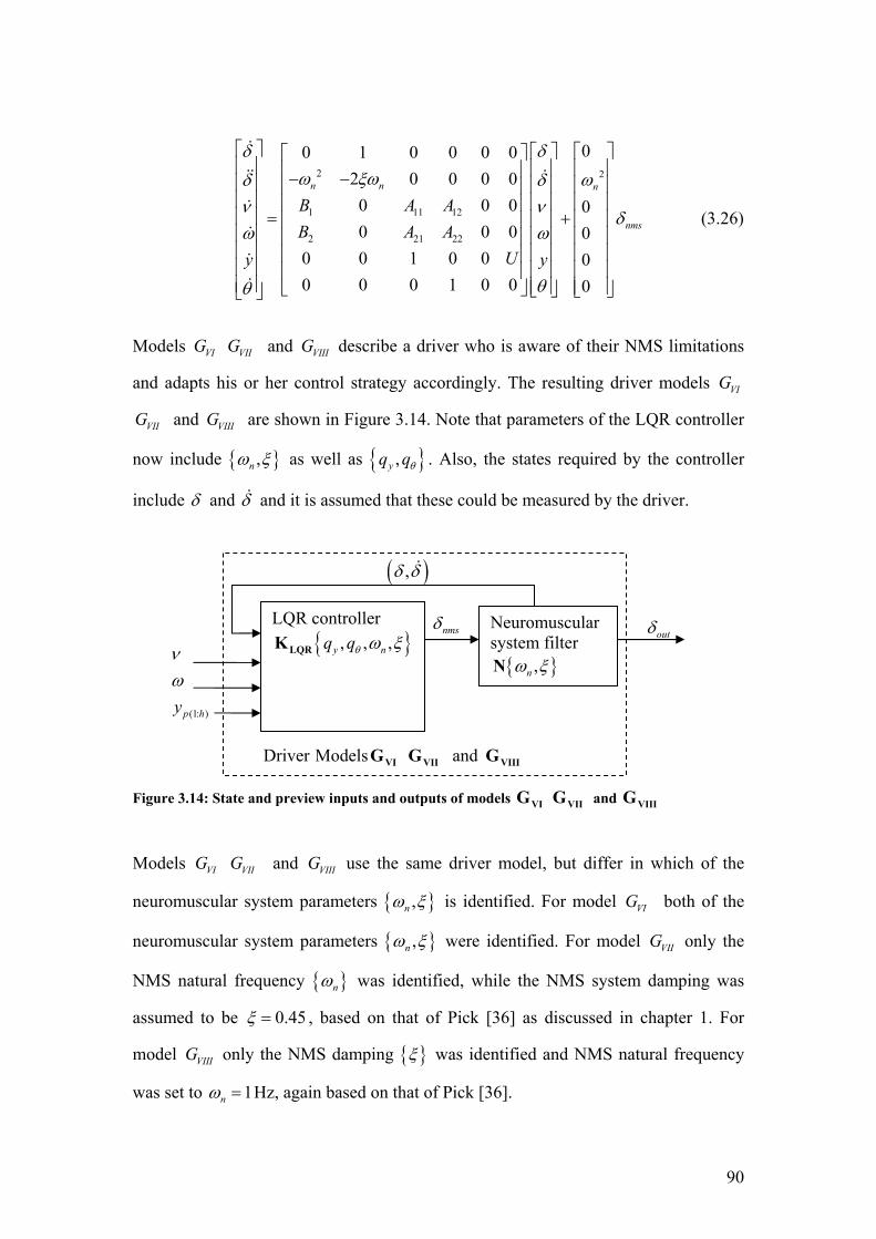
90
2 2
1 11 12
2 21 22
00 1 0 0 0 02 0 0 0 00 0 0 00 0 0 0
0 0 1 0 0 00 0 0 1 0 0 0
n n n
nms
B A AB A A
Uy y
δ δω ξω ωδ δ
ν νδ
ω ω
θθ
− − = +
(3.26)
Models VIG VIIG and VIIIG describe a driver who is aware of their NMS limitations
and adapts his or her control strategy accordingly. The resulting driver models VIG
VIIG and VIIIG are shown in Figure 3.14. Note that parameters of the LQR controller
now include { },nω ξ as well as { },yq qθ . Also, the states required by the controller
include δ and δ and it is assumed that these could be measured by the driver.
Figure 3.14: State and preview inputs and outputs of models VIG VIIG and VIIIG
Models VIG VIIG and VIIIG use the same driver model, but differ in which of the
neuromuscular system parameters { },nω ξ is identified. For model VIG both of the
neuromuscular system parameters { },nω ξ were identified. For model VIIG only the
NMS natural frequency { }nω was identified, while the NMS system damping was
assumed to be 0.45ξ = , based on that of Pick [36] as discussed in chapter 1. For
model VIIIG only the NMS damping { }ξ was identified and NMS natural frequency
was set to 1nω = Hz, again based on that of Pick [36].
(1: )p hy
νω
nmsδ Neuromuscular system filter { },nω ξN
outδ LQR controller { }, , ,y nq qθ ω ξLQRK
Driver Models VIG VIIG and VIIIG
( ),δ δ

91
3.3 Comparison of preview and state gains
The preview and state gains of models IG to VIIIG were evaluated to enable
comparison between them. The cost function weights used for the study are
{ } { }, 0.05,5yq qθ = for all models.
The NMS natural frequency nω was 1 Hz for models VG to VIIIG , consistent with the
0.9 Hz to 3.7 Hz range found by Pick [36]. The NMS damping for model VG was set
to 0.707ξ = to provide a NMS with attenuation, but no resonance. The NMS
damping for models VIG to VIIIG was set to 0.45ξ = which is consistent with Pick’s
value for relaxed limbs [36] and parameter values identified for this model in chapter
5. For model IVG , 4dN = was used corresponding to 0.2 seconds of delay, consistent
with values used by previous researchers [36, 39, 41] as discussed in section 3.1.2.
Vehicle parameters were the same as those used for simulator testing in chapter 5 and
are listed in appendix A. Preview time ( pT ) was 4 s, with 0.05 s timestep (T ), giving
80 preview points. Controllers were evaluated at both low speed (20 m/s) and high
speed (50 m/s) and are shown in sections 3.3.1 and 3.3.2 respectively.
3.3.1 Low speed controllers (20 m/s)
Preview and state gains for models IG to VIIIG were evaluated first at 20m/s, the
lowest speed used in testing in chapter 5. Preview gains against preview time for
models IG to IIIG are shown in Figure 3.15.

92
0 0.5 1 1.5 2 2.5 3 3.5 4−0.02
0
0.02
0.04
0.06
0.08
0.1
Preview Time (/s)
k pi (
/rad
m−
1 )G
IG
IIG
III
Figure 3.15: Preview gains for models IG to IIIG at 20 m/s with{ } { }y θq ,q = 0.05,5
Model IG shows that preview points further ahead of the vehicle have less
significance to the driver. Preview points closer to the vehicle have positive gain
(steering the ‘wrong’ way i.e. away from the direction of the curve), while points
further ahead have a negative gain (steering the ‘correct’ way i.e. towards the
direction of the curve).
This particular set of { },yq qθ weights gives a controller with preview gains
somewhere between what Sharp refers to as ‘heading error weighted’ and ‘steer angle
weighted’ cases. The controller tends to steer the correct way first (towards the curve)
as in the ‘steer angle weighted’ case, to cut corners and reduce steer angle effort.
However, it also steers the ‘wrong’ way (away from the curve) close to the driver as is
the case with ‘heading error weighted’ controller.
The preview gains for model IIG have similar shape to those for IG except for the 0.5
seconds nearest the vehicle. Very close to the vehicle, the preview points are much
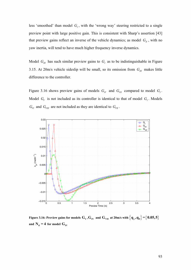
93
less ‘smoothed’ than model IG , with the ‘wrong way’ steering restricted to a single
preview point with large positive gain. This is consistent with Sharp’s assertion [43]
that preview gains reflect an inverse of the vehicle dynamics; as model IIG , with no
yaw inertia, will tend to have much higher frequency inverse dynamics.
Model IIIG has such similar preview gains to IG as to be indistinguishable in Figure
3.15. At 20m/s vehicle sideslip will be small, so its omission from IIIG makes little
difference to the controller.
Figure 3.16 shows preview gains of models IVG and VIIG compared to model IG .
Model VG is not included as its controller is identical to that of model IG . Models
VIG and VIIIG are not included as they are identical to VIIG .
0 0.5 1 1.5 2 2.5 3 3.5 4−0.015
−0.01
−0.005
0
0.005
0.01
0.015
0.02
0.025
0.03
Preview Time (/s)
k pi (
/rad
m−
1 )
GI
GIV
GVII
Figure 3.16: Preview gains for models IG , IVG and VIIG at 20m/s with { } { }y θq ,q = 0.05,5
and dN = 4 for model IVG

94
Model IVG has identical gains to model IG , but shifted forward by dN timesteps to
compensate for the delay in the driver, as previously observed by Pick [36]. It seems
intuitively correct that the driver should compensate for delay by looking further
ahead of the vehicle.
Model VIIG has broadly similar preview gains to IG , but the presence of a
neuromuscular system filter causes the preview gains to be ‘smoothed’, appearing
more sinusoidal than those of IG . These gains represent the inversion of the slightly
oscillatory NMS. Sharp [56] suggested that a sinusoidal variation of preview gains
may provide a form of feed-forward damping to compensate for the low damping in
the NMS. Also, the gains are shifted further ahead of driver, which will compensate
for the phase-delaying effect of the neuromuscular system.
In all cases, preview gain drops to zero well within the preview length, so assumption
of rotation into the driver reference frame (equation (3.16)) is valid.
Figure 3.17 shows the state gains kν and kω for all of the models. VG has the same
state gains as IG . Also shown are the kδ and kδ gains for model VIIG and the delay
state gains ( )dN ikδ − for model IVG . Model IIG has no state gains and model IIIG has
only kω .

95
I III IV VII0
0.2
0.4
0.6
0.8
G
k ω /(
rad/
(rad
s−1
))
I IV VII0
0.01
0.02
0.03
0.04
0.05
0.06
G
k ν /(
rad/
(m s−1
))
0
0.1
0.2
0.3
0.4
0.5
kδ kdδ/dt
(/s)
Sta
te g
ains
for
NM
S
GVII
0
0.05
0.1
0.15
0.2
kδ 4
kδ 3
kδ 2
kδ 1
GIV
Del
ay s
tate
gai
n k δ
Nd−
i
Figure 3.17: State gains for models IG to VIIG at 20 m/s, with{ } { }y θq ,q = 0.05,5 and
dN = 4 for model IVG
State gains for kν and kω are broadly similar for all models, with some up to 20%
higher than model IG . Pick [36] noted that the LQR state gains are analogous to the
compensatory controller gains of Weir and McRuer [40]. The similarity in state gains
for all models therefore implies that the compensatory controller gains are similar for
all of the driver models at 20 m/s.
Models IVG and VIIG have increased delay. In these models kω and kν are greater
than model IG and may help to increase damping of the vehicle motion in the
presence of the destabilising delay.
The steer angle delay state gains of model IVG are all of similar magnitude and
increase as the steer angle progresses down the shift register (at the end of which, it is
applied to the vehicle). Pick [36] suggested viewing this as a discrete filter on steer
angle.

96
3.3.2 High speed controllers (50 m/s)
Controllers IG to VIIG were then re-evaluated at 50 m/s (112 mph). The preview
gains of models IG to IIIG are shown in Figure 3.18 and models IG , IVG and VIIG in
Figure 3.19.
0 0.5 1 1.5 2 2.5 3 3.5 4−0.04
−0.02
0
0.02
0.04
0.06
0.08
0.1
Preview Time (/s)
k pi (
/rad
m−
1 )
GI
GII
GIII
Figure 3.18: Preview gains for models IG to IIIG at 50 m/s with { } { }y θq ,q = 0.05,5

97
0 0.5 1 1.5 2 2.5 3 3.5 4−0.02
−0.015
−0.01
−0.005
0
0.005
0.01
0.015
Preview Time (/s)
k pi (
/rad
m−
1 )G
IG
IVG
VII
Figure 3.19: Preview gains for models IG , IVG and VIIG at 50 m/s with { } { }y θq ,q = 0.05,5
and dN = 4 for model IVG
For all controllers preview gains as a function of time are of broadly similar shape to
those at 20m/s, but have shifted toward more negative gains such that the driver steers
more in the ‘correct’ direction i.e. toward a previewed curve. The fact that this has
happened to all models including IIG suggests that it is an effect of speed on the
‘track dynamics’ (those remaining in model IIG , equation (3.20)), rather than on the
vehicle dynamics.
For all models except IIG the preview gains fall to zero a shorter time ahead of the
vehicle at 50 m/s than at 20 m/s. This can be viewed as a reduction in preview time
from approximately 2.5 seconds at 20 m/s to approximately 2 seconds at 50 m/s.
Preview distance therefore increased from 50m to 100m. The preview length of model
IIG has remained nearly constant for both speeds, so this preview lengthening is
likely to be a vehicle dynamics effect, rather than a ‘track dynamics’ effect, because
IIG assumes a vehicle with no lateral or yaw dynamics. The fact that IIIG displays

98
increased preview length suggests that the increase may be due to a change in vehicle
yaw dynamics with speed.
At 20m/s the preview gains for model IIIG were nearly the same as IG , but this is not
the case at 50m/s. This suggests that sideslip ν is more significant at the higher
speed.
I III IV VII0
0.5
1
1.5
G
k ω /(
rad/
(rad
s−1
))
I IV VII0
0.02
0.04
0.06
0.08
0.1
G
k ν /(
rad/
(m s−1
))
0
0.2
0.4
0.6
0.8
kδ kdδ/dt
(/s)
Sta
te g
ains
for
NM
S
GVII
0
0.05
0.1
0.15
0.2
0.25
0.3
kδ 4
kδ 3
kδ 2
kδ 1
GIV
Del
ay s
tate
gai
n k δ
Nd−
i
Figure 3.20: State gains for models IG to VIIG at 50 m/s, with { } { }y θq ,q = 0.05,5 and
dN = 4 for model IVG
Figure 3.20 shows state gains for all models at 50m/s. For all models kν and kω are
related to each other in a similar way to the 20m/s gains, but are all approximately
twice the magnitude. Gains for states kδ and kδ for VIIG also double, as do the delay
state gains for IVG .
99
3.4 Comparison of closed loop driving
Models IG to VIIG are to be used to model drivers’ control of vehicles in closed loop.
A comparison of the closed loop control of each of the models IG to VIIG is therefore
made in this section. All models IG to VIIG were used to control the same plant: the 2
DOF vehicle model in equations (3.2) to (3.5). All models were compared with IG ,
which was used as the baseline case, since this has the LQR controller model equal to
the vehicle being controlled.
The road profile followed by each controller was the same, to allow direct
comparison. The profile was randomly generated, but band-limited by filtering.
Details of how this profile was generated are given in chapter 4. Each model IG to
VIIG was ‘driven’ at both 20 m/s and 50 m/s.
Each model was run with and then without a delay (τ ) of 0.2 seconds incorporated
into the closed loop. This was to test how realistically each driver model could cope
with the unavoidable delays present in the driver. A delay of 0.2 seconds is consistent
with that used by other researchers [36, 39, 41] as discussed in section 3.1.2.
Section 3.4.1 describes the simulation method for closed loop modelling, then each
model’s performance is described in sections 3.4.3 to 3.4.7.
3.4.1 Simulation method
Closed loop vehicle simulation was carried out in MATLAB using a discrete time
model. Time steps were 0.05T = seconds, fast enough to represent the vehicle
dynamics, but without creating too many preview points. Creating too many preview
points tends to slow down the calculation of the LQR controller in MATLAB to a
prohibitive degree. Closed loop simulation involves four parts as shown in Figure

100
3.21, namely the driver model, vehicle model, trajectory algorithm and preview offset
algorithm.
Figure 3.21 shows the driver model G outputting steer angle δ to the vehicle model
( )F q , from which vehicle states ( ), ,ν ω θ are fed back to the driver and to the
trajectory calculation algorithm. The Trajectory algorithm calculates current vehicle
position ( ),v vx y from vehicle states ( ), ,ν ω θ . The vehicle position ( ),v vx y and the
track input ( )t tx , y are then used by the Preview algorithm to calculate the preview
offsets (1: )p ny which in turn are used by the driver model G to calculate steer angle
δ .
Figure 3.21: Generalised model of closed loop simulation, showing appropriate feedback for model IG
The driver model G was described in the previous sections and once its preview and
state gains are determined, involves only the evaluation of equation (3.16) each time
step. The preview offset algorithm is described in sections 3.4.2. Each driver model
IG to VIIG has different states fed back so a diagram of the closed loop system for
each of IG to VIIG is included in sections 3.4.3 to 3.4.7.
The vehicle model used for simulation is the bicycle model shown in equations (3.2)
to (3.5) and Figure 2.3. The state space vehicle model was discretised using
MATLAB’s C2D function with a time step of 0.05T = s.
( ),v vx y
Driver Model G
(1: )p ny δ
Vehicle model
( )F q
Trajectory algorithm { }f U ( ), ,ν ω θ
( ),ν ω
Preview algorithm { }f U
( )t tx , y
101
The vehicle trajectory algorithm shown in Figure 3.21 is defined in equation (3.27).
Vehicle trajectory is calculated in global co-ordinates ( ),v vx y as shown in Figure
3.22.
( ) cos ( ) sin ( )( ) sin ( ) cos ( )
v
v
x t U t ty t U t t
θ ν θθ ν θ
= −= +
(3.27)
Numerical integration is then used to establish vehicle position ( ),v vx y .
In reality there would be noise present within the control loop when a driver controls
a real vehicle, but for ease of comparison this is omitted from simulations in this
chapter. Driver noise and its consequences are discussed in chapter 4. Weights on
lateral and heading errors were set to { } { }, 0.05,5yq qθ = as in the previous section.
3.4.2 Preview offset algorithm
The preview offset algorithm is designed to operate under the same small angle
approximation inherent in the linearised discrete track equation (3.6). However, some
curves will exceed these small angles and the algorithm must be robust to this. The
preview offset algorithm also deals with the problem of interpolating road path data
points of arbitrary spacing. The algorithm used is as follows:
1. Cartesian representation of the track ( )t tx , y in the global reference frame is
rotated into the vehicle reference frame as shown in Figure 3.22 using equation
(3.28).
( ) ( ( )) cos ( ) ( ( ))sin ( )( ) ( ( ))sin ( ) ( ( )) cos ( )
t v v
t v v
t x t t y t tt y t t y t t
θ θθ θ
= − + −= − − + −
t t
t t
x x yy x y
(3.28)
Where ( )t tx , y represents two column vectors of track position points ( ),ti tix y in
the global reference frame. Also ( )( ), ( )v vx t y t represents the current vehicle
position in global co-ordinates and ( )tθ represents the vehicle’s current yaw
angle.

102
Figure 3.22: Global and vehicle reference frames for expressing track location. Preview points equally spaced along track are illustrated
2. The point on the road path perpendicular to the vehicle is established (the point at
0x = in the vehicle ref. frame). Interpolation was used as there will not be a point
exactly at 0x = (brackets { } denote interpolation).
{ }{ }
0
0
0
0p t t
p t t
y y x
S S x
= =
= = (3.29)
An array of points is generated equally spaced along the track, starting at 0pS (the
point perpendicular to vehicle). 0.05T = s is the time step used to discretise the
LQR controller.
0pi pS S UTi= + (3.30) 3. Cartesian positions ( ),pi pix y of the array of points defined by equation (3.30) are
interpolated at these locations along the track ( tS is same for both reference
frames):
{ }{ }
pi t t pi
pi t t pi
x x S S
y y S S
= =
= = (3.31)
0py
x
y
x
UT
UT
UT ( ),pi pix y
θ
( ),v vx y
0pS
1pS y

103
This gives rise to a two column vector of Cartesian positions ( )pi pix , y of the
previewed points on the path which are equally spaced along the path a distance
UT apart as shown in Figure 3.22. These previewed points can be joined with
straight sections of track as shown in Figure 3.23.
4. Angles between the straight sections of track shown in Figure 3.23 are determined
from the list of Cartesian positions ( )pi pix , y (in vehicle reference frame) as
shown in Figure 3.23 and equation (3.32).
1
1
arctan i ipi
i i
y yx x
ψ −
−
−= −
(3.32)
Figure 3.23: Small angle approximation method for preview offset determination, applied to case with large angles
5. Preview offsets pny are then determined from the angles between these discrete
sections using a small angle approximation:
0 01 1
n n
pn p pi p pii i
y y y y UTψ= =∑ ∑= + ∆ = + (3.33)
0py
x
y
x
1pψ
piψ
piy∆
1py∆ 2pψ 2py∆

104
This procedure is repeated every time step to establish new preview offsets. Equation
(3.33) is based on the same small angle assumption as the track model (equation (3.6))
so is consistent with way the LQR controller model is formulated. The algorithm
above avoids the problem which can arise if preview points are spaced equally along
the preview optical lever, instead of along the track. If preview points are spaced
evenly along the preview lever, then infinite preview offsets can arise, for example
when previewing a 90° bend as shown in Figure 3.24.
Figure 3.24: Problem of infinite preview offset when preview points are evenly spaced along the preview lever
3.4.3 Model IIG
Model IIG was simulated in closed loop with the 2DOF bicycle model. The system is
shown in Figure 3.25. Note that a delay block was added to driver model of Figure 3.8
which shifts the steer angle by a whole number of time steps to represent the driver’s
internal delay τ .
0py 1py
2py 3py = ∞

105
Figure 3.25: Closed loop driving of model IIG with possibility of delay
Poor control was expected for IIG for two reasons. Firstly only preview information
is fed back to the driver model IIG , (no vehicle states) so all of the feedback
information to the driver must pass through the integration within the trajectory
algorithm. In the trajectory algorithm sideslip velocity ν and yaw rate ω are
integrated to give position ( , )v vx y and yaw angle θ . This feedback path will
therefore have more phase lag than direct feedback of sideslip velocity and yaw rate.
Secondly the LQR controller for model IIG is derived from a simplification of the
vehicle so will not be optimal for the vehicle ( )F q .
The steer angle of driver model IIG operating in closed loop with the vehicle was
compared with that of model IG . Model IG was shown in closed loop with the
vehicle in Figure 3.21. Model IG also includes a delay τ in series with the LQR
controller shown in Figure 3.4.
Figure 3.26 shows a comparison of steer angle vs. distance of model IG and IIG on
the same track. The model was operated in four configurations; two speeds,
20U = m/s and 50U = m/s; and two delay settings, 0τ = and 0.2τ = seconds (4 time
steps). For all models in this section, the left hand plots show the case with zero delay
( 0τ = ) and the right hand plots with delay 0.2τ = s. The upper plots show 20m/s and
Driver Model IIG
LQR controller
{ },yq qθLQRK
(1: )p hy δ
Vehicle model F(q)
Trajectory algorithm { }f U ( ), ,ν ω θ
( ), ,v vx y θ
Delay τ
Preview algorithm { }f U
( )t tx , y

106
the lower plots 50m/s. The controllers IG and IIG for these two speeds were shown
in section 3.3.
Figure 3.26: Steer angle vs. time for model IIG and model IG on same random track ( )t tx , y .
Left hand plots show τ = 0 , right hand plots τ = 0.2 . Upper plots U=20m/s, lower plots U=50m/s
At low speed ( 20U = m/s), both controllers IIG and IG give similar steer angles.
With no delay ( 0τ = ), model IIG has slightly more overshoot than IG , which would
lead to slightly poorer control of the vehicle. With 0.2τ = s at 20U = m/s both
controllers generate more steer angle for a given point in the track. Also IIG and IG
both show more overshoot in their steer angle output with delay present. Model IIG
gives slightly more overshoot than model IG , perhaps because it has no state gains to
provide yaw rate feedback.
800 1000 1200 1400−30
−20
−10
0
10
20
30
40τ=0, U=20 m/s
Ste
er a
ngle
/°
800 1000 1200 1400−30
−20
−10
0
10
20
30
40τ=0.2s, U=20 m/s
800 1000 1200 1400
−60
−40
−20
0
20
40
60
τ=0, U=50 m/s
Ste
er a
ngle
/°
Track distance /m800 1000 1200 1400
−60
−40
−20
0
20
40
60
τ=0.2s, U=50 m/s
Track distance /m
GI
GII
GI
GII
GI
GII
GI
GII

107
At high speed ( 50U = m/s), the closed loop responses for IIG and IG are quite
different from their counterparts at low speed. Firstly comparing model IG to its
performance at low speed, the steer angle δ resembles a low-pass filtered version of
the steer angle at low speed, with fewer short wavelength steer angle inputs. This is a
result of the longer preview length at 50U = m/s as discussed in section 3.3.2.
With no delay ( 0τ = ) and at high speed ( 50U = m/s), the steer angle for model IIG
is quite different to that of IG . The steer angles for IIG appear to be delayed from
those of IG . This is a result of the shorter length of preview for model IIG (Figure
3.18) leading to later steering for a given feature in the track. This in turn gives poorer
closed loop control of the system, leading to much larger steer angles for IIG than for
IG .
With delay 0.2τ = s, model IIG is unstable in closed loop control. Although
instability in a steering controller is undesirable, the modelled behaviour could
conceivably be consistent with that of a poor human driver.
3.4.4 Model IIIG
Model IIIG is the next most sophisticated driver model and performance should be
better than IIG because yaw rate feedback is included. As discussed in section 3.3.1
model IIIG has a very similar controller to IG at low speed. Similar results would
therefore be expected at 20U = m/s, but not necessarily at 50U = m/s. Figure 3.27
shows a diagram of closed loop control with model IIIG .

108
Figure 3.27: Model IIIG operating in closed loop, including delay
Figure 3.28 shows steer angle vs. distance for models IIIG and IG , with 0τ = and
0.2τ = s. The upper two plots are at 20 m/s, the lower at 50 m/s.
Driver Model IIIG ( ),v vx y
(1: )p hy δ
Vehicle model F(q)
Trajectory algorithm { }f U
( ), ,ν ω θ
ω
LQR controller
{ },yq qθLQRKDelay τ
Preview algorithm { }f U
( )t tx , y

109
Figure 3.28: Steer angle vs. time for model IIG and model IG on same random track ( )t tx , y .
Left hand plots show τ = 0 , right hand plots τ = 0.2 . Upper plots U=20m/s, lower plots U=50m/s
At low speed the controllers IIIG and IG show almost identical performance with and
without delay, as predicted. The high speed cases again show an apparent delay in
steering between IIIG and IG . The amount of delay is consistent with the slightly
shorter preview time used by IIIG than IG .
The simplification of the controller IIIG from that of IG has only degraded its
performance at high speed, where sideslip velocity (ν ) becomes important. Model
IIIG is able to keep control of the vehicle even with delay 0.2τ = s, assisted by yaw
rate feedback (which was not present for IIG ). Also, for IIIG the vehicle model on
800 1000 1200 1400−30
−20
−10
0
10
20
30
40τ=0, U=20 m/s
Ste
er a
ngle
/°
800 1000 1200 1400−30
−20
−10
0
10
20
30
40τ=0.2s, U=20 m/s
800 1000 1200 1400
−60
−40
−20
0
20
40
60
τ=0, U=50 m/s
Ste
er a
ngle
/°
Track distance /m800 1000 1200 1400
−60
−40
−20
0
20
40
60
τ=0.2s, U=50 m/s
Track distance /m
GI
GIII
GI
GIII
GI
GIII
GI
GIII
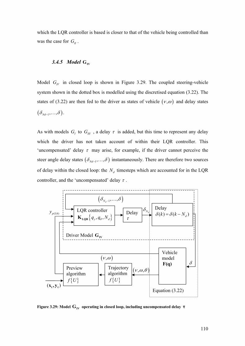
110
which the LQR controller is based is closer to that of the vehicle being controlled than
was the case for IIG .
3.4.5 Model IVG
Model IVG in closed loop is shown in Figure 3.29. The coupled steering-vehicle
system shown in the dotted box is modelled using the discretised equation (3.22). The
states of (3.22) are then fed to the driver as states of vehicle ( ),ν ω and delay states
( )1, ,Ndδ δ− … .
As with models IG to IIIG , a delay τ is added, but this time to represent any delay
which the driver has not taken account of within their LQR controller. This
‘uncompensated’ delay τ may arise, for example, if the driver cannot perceive the
steer angle delay states ( )1, ,Ndδ δ− … instantaneously. There are therefore two sources
of delay within the closed loop: the dN timesteps which are accounted for in the LQR
controller, and the ‘uncompensated’ delay τ .
Figure 3.29: Model IVG operating in closed loop, including uncompensated delay τ
Driver Model IVG
Trajectory algorithm { }f U
( ), ,ν ω θ
LQR controller { }, ,y dq q NθLQRK
dNδ
Equation (3.22)
Vehicle model F(q)
Delay ( ) ( )dk k Nδ δ= −
δ( ),ν ω
( )1, ,dNδ δ− …
(1: )p hy Delay τ
Preview algorithm { }f U
( )t tx , y

111
Figure 3.30 shows the steer angles of model IVG compared with those of IG . Model
IVG is shown with 4dN = (corresponding to 0.2 seconds of delay) in all four plots.
Note that model IVG with 0dN = would be the same as model IG , but this case is not
shown here.
Figure 3.30: Steer angle vs. time for model IVG and model IG on the same random track
( )t tx , y . Left hand plots show τ = 0 for both models with dN = 4 . Right hand plots
τ = 0.2 s for both models with dN = 4 . Upper plots at U = 20 m/s, lower plots at U = 50 m/s
For all four plots of Figure 3.30 the steer angles of models IG and IVG are nearly
identical, despite IVG having an extra 4dN = steps of time delay within the closed
loop. This means that the LQR controller has been able to nearly perfectly
compensate for the delay dN by shifting its preview points forward in time (Figure
800 1000 1200 1400−30
−20
−10
0
10
20
30
40τ=0, U=20 m/s
Ste
er a
ngle
/°
800 1000 1200 1400−30
−20
−10
0
10
20
30
40τ=0.2s, U=20 m/s
800 1000 1200 1400
−60
−40
−20
0
20
40
60
τ=0, U=50 m/s
Ste
er a
ngle
/°
Track distance /m800 1000 1200 1400
−60
−40
−20
0
20
40
60
τ=0.2s, U=50 m/s
Track distance /m
GI
GIV
GI
GIV
GI
GIV
GI
GIV
112
3.19) and by including the steer angle delay states ( )1, ,Ndδ δ− … . The similarity
between IG and IVG is clear for both values of τ and for both speeds.
Slight differences are visible between the steer angles of IG and IVG for all four cases
in Figure 3.30. This is because IVG will have an extra dN steps of time delay in its
state feedback information ( ),ν ω compared with model IG . This effect was
anticipated by Pick [36] when deriving this controller. The extra delay in state
feedback does not seem to significantly degrade the controller performance even at
high speed.
3.4.6 Model VG
In model VG the driver does not take account of the NMS in their formulation of the
LQR controller. As with model IIG , this case has significant mismatch between the
LQR controller and the coupled NMS-vehicle system being controlled. Also the
introduction of an NMS will increase phase lag in the closed loop and reduce
bandwidth of control. For both of these reasons poor performance might be expected.

113
Figure 3.31: Model VG operating in closed loop, including delay τ
Figure 3.31 shows closed loop operation of model VG . States passed to the driver
model are both of the vehicle states ( ),ν ω as for IG , but none of the neuromuscular
system states. When simulating the system in closed loop, the neuromuscular system
filter N is coupled to the vehicle state space model in a similar way to equation (3.26)
. The state space model of the filter N is given by equations (3.34) to (3.36).
2 2
00 12 nms
n n n
δδδ
ω ξω ωδδ
= + − −
(3.34)
[ ] [ ]out lead lead lead nmsa b cδ
δ δδ
= +
(3.35)
Where:
2
2
1
2
nlead
cut
nlead cut
cut cut
nlead
cut
a
b
c
ωω
ωξ ξω ω
ωω
= −
= −
=
(3.36)
Driver Model VG
(1: )p hy
Trajectory algorithm { }f U
( ), ,ν ω θ
LQR controller { },yq qθLQRK
nmsδ Equation (3.37)
Vehicle model F(q)
Neuromuscular system filter { },nω ξN
outδ ( ),ν ω
Delay τ
Preview algorithm { }f U
( )t tx , y

114
This state space model is then coupled with the vehicle state space model of equation
(3.4) to give equation (3.37). A discretised version of the coupled vehicle-NMS
system in equation (3.37) is used in the MATLAB simulation to model the part of the
system shown in the dotted box of Figure 3.31. This method is also used for
simulation of model VIIG in section 3.4.7.
2 2
1 1 11 12 1
2 2 21 22 2
00 1 0 0 0 02 0 0 0 0
0 00 0
0 0 1 0 0 00 0 0 1 0 0 0
n n n
lead lead leadnms
lead lead lead
a B b B A A c Ba B b B A A c B
Uy y
δ δω ξω ωδ δ
ν νδ
ω ω
θθ
− − = +
(3.37)
The steer angle time history of model VG is compared with that of model IG in
Figure 3.32.

115
Figure 3.32: Steer angle vs. time for model VG and model IG on same random track ( )t tx , y .
Left hand plots show τ = 0 , right hand plots τ = 0.2 . Upper plots U=20m/s, lower plots U=50m/s
At low speed ( 20U = m/s ) with no delay ( 0τ = ), steer angle only overshoots mildly
from that of model IG . However, when the delay 0.2τ = s is introduced, the steer
angle of model VG becomes very oscillatory compared to model IG . This is due to
the destabilising effect of the phase delay from the neuromuscular system, which is
not present in IG .
At high speed ( 50U = m/s), oscillatory steering is evident even without delay in the
loop ( 0τ = ). When delay 0.2τ = s is introduced, the closed loop is unstable. From
these results it seems unlikely that a driver could adequately control a car without
800 1000 1200 1400−30
−20
−10
0
10
20
30
40τ=0, U=20 m/s
Ste
er a
ngle
/°
800 1000 1200 1400−30
−20
−10
0
10
20
30
40τ=0.2s, U=20 m/s
800 1000 1200 1400
−60
−40
−20
0
20
40
60
τ=0, U=50 m/s
Ste
er a
ngle
/°
Track distance /m800 1000 1200 1400
−60
−40
−20
0
20
40
60
τ=0.2s, U=50 m/s
Track distance /m
GI
GV
GI
GV
GI
GV
GI
GV

116
adjusting the cost function weights to improve high speed stability, or using a more
sophisticated LQR controller such as model VIIG , as shown in the next section.
3.4.7 Models VIG VIIG and VIIIG
Models VIG , VIIG and VIIIG form the same closed loop system shown in Figure 3.33.
Figure 3.33: Models VIG VIIG and VIIIG operating in closed loop, including delay τ
For models VIG , VIIG and VIIIG , as well as vehicle states ( ),ν ω , the NMS states δ and
δ are passed to the driver model. As for VG , a discretised version of the state space
model in equation (3.37) is used for MATLAB simulation of the coupled NMS-
vehicle system shown in the dotted box. Figure 3.34 shows the steer angle
performance of model VIIG and IG .
Driver Model VIG , VIIG and VIIIG
(1: )p hy
Trajectory algorithm { }f U
( ), ,ν ω θ
LQR controller { }, , ,y nq qθ ω ξLQRK
nmsδ Equation (3.37)
Vehicle model F(q)
Neuromuscular system filter { },nω ξN
outδ ( ),ν ω
( ),δ δ
Delay τ
Preview algorithm { }f U
( )t tx , y

117
Figure 3.34: Steer angle vs. time for model VIIG and model IG on same random track
( )t tx , y . Left hand plots show τ = 0 , right hand plots τ = 0.2 . Upper plots U=20m/s, lower plots U=50m/s
Figure 3.34 shows that for both low speed ( 20U = m/s) and high speed ( 50U = m/s)
without delay ( 0τ = ), the steer angle of model VIIG is almost identical to model IG .
The inclusion of the NMS within the LQR controller has enabled the driver to nearly
fully ‘compensate’ for the effect of the NMS that was evident in model VG . This is
achieved by the feedback of NMS states and the shifting forward of the preview
gains. If delay 0.2τ = s is included at high speed ( 50U = m/s), only a slight
difference in steer angles between VIIG and IG can be seen.
800 1000 1200 1400−30
−20
−10
0
10
20
30
40τ=0, U=20 m/s
Ste
er a
ngle
/°
800 1000 1200 1400−30
−20
−10
0
10
20
30
40τ=0.2s, U=20 m/s
800 1000 1200 1400
−60
−40
−20
0
20
40
60
τ=0, U=50 m/s
Ste
er a
ngle
/°
Track distance /m800 1000 1200 1400
−60
−40
−20
0
20
40
60
τ=0.2s, U=50 m/s
Track distance /m
GI
GVII
GI
GVII
GI
GVII
GI
GVII

118
3.5 Conclusions
A requirement was identified in chapter 2 for a driver model which includes a steering
strategy parameter, so models of the driver were developed based on Sharp’s LQR
controller structure. The models included cost function weights to allow the driver’s
strategy to be altered in favour of lateral error minimisation, heading error
minimisation, or steer angle minimisation. In chapter 1 the need was identified for
models to represent the novice driver, and to incorporate the effect of the NMS into
the driver’s internal model. A driver model with simplified vehicle dynamics has been
developed to represent novice drivers, and a range of models including the driver’s
neuromuscular system have also been developed. The preview and state gains of the
controllers developed in this chapter have been compared as well as their steer angles
in closed loop driving. The important features of each model were:
Model IG used an LQR controller based on Sharp’s 2DOF bicycle model. The closed
loop steer angles for model IG during high speed driving resembled a low pass
filtered version of its steer angles at low speed. This is because the preview length of
the high speed controller was double that of the low speed controller. Adding a delay
0.2τ = s within the closed loop increased the steer angle used.
Model IIG used an LQR controller based on a point mass model to represent a novice
driver. Model IIG had abrupt changes in its preview gains with preview time because
the vehicle model had no yaw dynamics. Model IIG gave closed loop steer angles
similar to IG at low speed, but was unstable at high speed in the presence of delay
( 0.2τ = s), possibly due to its lack of a yaw rate state gain.
Model IIIG used an LQR controller based on a single degree of freedom second order
model with no sideslip so only the yaw rate state is fed back to the driver. Model IIIG
gave closed loop steer angles very similar to IG at low speed but at high speed, steer
angles resembled those of IG ‘delayed’ due to preview being shorter.

119
Model IVG used an LQR controller with delay states. Model IVG with 4dN = gave
nearly identical steer angles to IG for both 20U = m/s and 50U = m/s and for both
0τ = and 0.2τ = s. Preview shifting and steer angle delay state gains were able to
nearly completely compensate for the delay dN .
Model VG used the same 4 state LQR controller as model IG , but its output steer
angle was filtered through an NMS. Model VG gave more oscillatory closed loop
steer angles than IG . At high speed in the presence of the delay 0.2τ = s the closed
loop controller VG was unstable.
Models VIG , VIIG and VIIIG used a six state LQR controller based on a coupled
vehicle and neuromuscular system model and an NMS filter on its output steer angle.
Model VIIG was able to closely reproduce model IG ’s performance despite the NMS
filter being present within the closed loop. This was due to the NMS state gains and
the preview shifting.
Increasing vehicle speed from 20m/s to 50 m/s doubled the state gains of all
controllers and shifted preview gains toward more negative values corresponding to
steering more toward the direction of a curve. Increasing speed from 20 to 50 m/s also
reduced the preview time of all controllers due to changes in vehicle dynamics.

120
Chapter 4: Identification of driver steering models
In this chapter, the procedure for identification of driver models from recorded data is
explained and validated. In the first half of the chapter, two possible methods for
identification of the driver model are explained, namely the direct, and indirect
methods. The direct method was chosen for further development and the algorithms
developed for driver identification using the direct method are described. The second
half of the chapter describes the way in which the direct method was validated by
identifying models from artificially created data. Validation of the method for each of
the models in chapter 3 is described, and a study of the available parameters is carried
out. This parameter study assisted in the design of the identification experiment to be
carried out on drivers in chapter 5.

121
4.1 Identification procedure
In the previous chapter, each of the controllers IG to VIIIG was operated in closed
loop to investigate its performance, however, in order for these models to represent a
driver more accurately, they must be modified to include the noise inherent in a
driver’s control [24]. This driver internal noise may have many sources e.g.
inaccuracies in the reproduction of intended steer angle by the neuromuscular system;
or noise arising from misperception of system parameters (preview offsets, or vehicle
states). All of these sources can be modelled together by ‘referring’ the noise to the
driver’s output (steer angle δ ) as a random coloured additive noise signal as shown in
Figure 4.1.
Figure 4.1: Driver-vehicle closed loop system including added driver noise η(t)
In Figure 4.1, driver noise is represented by a coloured noise signal ( )tη which is
produced from a white noise signal ( )e t , filtered with a noise filter ( )H q . For the
driver system, ( )r t represents the road path input, ( )G q is the driver model, and
( )F q is the vehicle model.
The method used for identification of G must be chosen to take account of the noise
(η ) entering at a point within the closed loop. Ljung [47] describes two methods for
Actual driver- vehicle system
( )G q
( )F q
( )H q
r(t) +
e(t)
( )tη
( )tδ
u(t)
n(t)
+
-
+
122
identification of such systems based on the prediction error method (PEM), namely
the direct, and indirect methods. Both methods involve comparing output (steer
angleδ ) recorded from the driver during simulator tests, to the output ( 'δ ) from a
proposed driver model which is subject to the same inputs. A suitable model of the
driver can then be found by choosing model parameters which give the minimum
prediction error ( 'δ δ− ). The two methods differ in whether they operate the driver
model ( 'G ) in open or closed loop. In the following sections 4.1.1 and 4.1.2, the
direct and indirect methods are explained, and the choice of the direct method is
justified in section 4.1.3.
4.1.1 Indirect method
The indirect method of system identification reported by Ljung [47] is shown in
Figure 4.2. In this method, the ‘actual driver-vehicle system’ output δ is compared to
the output 'δ from a ‘modelled driver-vehicle system’ (see Figure 4.2). The
‘modelled driver-vehicle system’ consists of a driver model estimate '( )G q operating
in closed loop with a vehicle model ( )F q . The input to the closed loop system ( )r t is
the same as was experienced by the actual driver during testing. This ‘modelled
driver-vehicle system’ contains no noise (see Figure 4.2), so is similar to the closed
loop models of chapter 3.

123
Figure 4.2: Indirect method identification of driver-vehicle closed loop system
For the ‘actual driver-vehicle system’ in Figure 4.2:
( ) ( ) ( ) ( ) ( ) ( ) ( ) ( ) ( ) ( ) ( ) ( )t G q u t H q e t G q r t G q F q t H q e tδ δ= + = − + (4.1)
Hence:
f fGS r HS eδ = + (4.2)
Where fS is the sensitivity function:
11fS
GF=
+ (4.3)
The steer angle 'δ of the modelled driver-vehicle system is given by:
' ' ' ' 'fG u G S rδ = = (4.4)
Actual driver- vehicle system
Modelled driver-vehicle system
u(t) ( )tη+
( )G q
( )F q
( )H q
r(t) +
e(t)
( )tδ
n(t)
'( )G q '( )tδ
( )F q
'( )u t
'( )n t
-
+
-
+
124
Where 'fS is the sensitivity function:
1'1 'fS
G F=
+ (4.5)
Prediction error ( )υ is therefore:
' ' ' ( ' ')f f fGu G u He GS G S r HS eυ δ δ= − = − + = − + (4.6)
A weighted prediction error ε is given by:
( ) ( ) ( ) ( ) ( )1 1 1' ' ' ' ' ' ' ' 'f f f f f fH S H S GS G S r H S HS eε δ δ
− − −= − = − + (4.7)
Where 'H and 'fS are estimates of the initially unknown H and fS . The weighting
of prediction error ( )υ using ( ) 1' 'fH S
− causes the noise term ( ) 1
' 'f fH S HS e−
to
approximate white noise. The purpose of adding this frequency weighting is to
minimise the misidentification of the driver model 'G , also known as bias.
Ljung [47] states that if the input ( )r and noise ( )e are uncorrelated, then minimising
the variance of ε will minimise ( ) ( )1' ' ' 'f f fH S GS G S
−− . The resulting estimate 'G
is given by [47]:
22
' 2'' arg min
1 ' 'f r
G
SG GG dFG H
π
πω
−∫
Φ−=
− (4.8)
Where arg min ( )x f x is the value of x that minimises ( )f x , and rΦ is the spectrum
of the input ( )r t . The ‘model set’ is the range of possible driver models used in the
optimisation of equation (4.8) to give the estimate 'G . The estimate 'G will be a
compromise between making 'G close to G , and making ( )1 1 'FG− small.
However, if the true system ( G ) exists within the model set, then the bias of the
system estimate 'G will be zero.
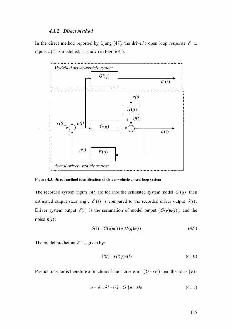
125
4.1.2 Direct method In the direct method reported by Ljung [47], the driver’s open loop response δ to
inputs ( )u t is modelled, as shown in Figure 4.3.
Figure 4.3: Direct method identification of driver-vehicle closed loop system
The recorded system inputs ( )u t are fed into the estimated system model '( )G q , then
estimated output steer angle '( )tδ is compared to the recorded driver output ( )tδ .
Driver system output ( )tδ is the summation of model output ( ( ) ( )G q u t ), and the
noise ( )tη :
( ) ( ) ( ) ( ) ( )t G q u t H q e tδ = + (4.9)
The model prediction 'δ is given by:
'( ) '( ) ( )t G q u tδ = (4.10)
Prediction error is therefore a function of the model error ( )'G G− , and the noise ( )e :
( )' 'G G u Heυ δ δ= − = − + (4.11)
Actual driver- vehicle system
( )H q
u(t) ( )G q
( )F q
( )tδ
n(t)
Modelled driver-vehicle system
( )tη
'( )G q '( )tδ
r(t)
e(t)
+
+
-
+
126
In the special case of white driver noise ( 1H = ), 'G can be determined by
minimising prediction error (υ ), and no bias would result. However, if driver noise
( He ) is non-white ( 1H ≠ ), minimising prediction error (υ ) would lead to bias in 'G .
For 1H ≠ a weighted prediction error ε must be minimised to reduce bias:
( ) ( )1 1 1 1' ' ' ' ' 'H H H G G u H Heε υ δ δ− − − −= = − = − + (4.12)
The prediction error (υ ) is weighted by an inverse noise model 1'H − , which must be
estimated to ensure that ( 1'H He− ) is white noise. However, even if 'H is a good
estimate, minimising ε does not minimise the error in the model 'G , because ε is
correlated with e via the closed loop. Ljung [47] states that minimising ε leads to the
following estimate of 'G :
( ) ( ) ( ) ( )( )
2
' 2' arg min ''u
GG G B G dH
π
π
ωω ω ω ω
ω−∫
Φ= + − (4.13)
Where uΦ is the spectrum of ( )u t and the bias term ( )B ω is given by:
( ) ( )( )
( )( ) ( ) ( )
22 2( )
'eu
u u
eB H H
σ ωω ω ω
ω ωΦ
= −Φ Φ
(4.14)
Where ( )eu ωΦ is the spectrum of the input ( )u t resulting from noise ( )e t fed back
through the vehicle. Identification bias ( ( )B ω ) in the frequency range of interest will
be small if either (or all) of the following hold:
1. The noise model is good ( 'H H− is small).
2. The feedback contribution to the input spectrum ( ( )( )
eu
u
ωω
ΦΦ
) is small.
3. The signal to noise ratio is good ( ( )( )
2( )
u
eσωΦ
is small).
These three conditions will need to be satisfied for a successful identification
experiment. Note from equation (4.13) that the identified model 'G is frequency
weighted by 2'u HΦ (called the prediction ‘norm’). This frequency weighting is

127
dependent on the input spectrum uΦ , and on the estimated noise model 'H . Although
the input spectrum uΦ can be designed as part of the experiment, the noise model 'H
is dependent on the driver’s internal noise colour H and so cannot be specified
freely.
4.1.3 Choice of identification method
The direct method was chosen to identify the driver models from experimental data.
The direct method was chosen as it used significantly less CPU time due to simulating
the ‘modelled driver-vehicle system’ (Figure 4.3) in open loop rather than in closed
loop (Figure 4.2). It was possible for the direct method to be just as accurate (bias
free) as the indirect method if the conditions set out in section 4.1.2 were met.
In the driver models IG to VIIIG there were additional feedback loops for the states
( )1 1, , , , , ,Ndν ω δ δ δ δ− … which were not considered in Ljung’s derivation. Validation
was undertaken to ensure that these extra feedback loops did not introduce bias into
the identification procedure. This validation is reported in section 4.2. The
identification procedure developed using Ljung’s direct method is described in section
(4.1.4).
4.1.4 Identification procedure
Direct method identification was carried out using the equations of the previous
section with an algorithm written in MATLAB. Validation of the identification
procedure is described in section 4.2. The procedure consists of two processes;
optimum model ( 'G ) selection as in equation (4.13), and noise model ( 'H )
identification. These processes are covered in section 4.1.4.1 and 4.1.4.2 respectively.
The complete identification algorithm is then explained in section 4.1.4.3.

128
4.1.4.1 Optimum model selection
Optimum model selection is summarised by equation (4.13). A minimisation search
function available in MATLAB (fminsearch) was used to perform the optimisation.
The function was used to find the model parameter estimates { ', ', '}yq qθ τ which
minimised ( )εΞ , the RMS of the weighted prediction error ε (defined in (4.12)) as
shown in (4.15). The parameters { , , }yq qθ τ were defined in chapter 3 for the driver
models IG to VIIIG .
( ) { }( ),', ', ' fminsearch , , '
yy q q yq q q q Hθθ θτ ε = Ξ (4.15)
The optimum time delay ( 'τ ) was not found by including it as a parameter of the
‘fminsearch’ optimisation. Instead 'τ was determined for each { , , '}yq q Hθ point
evaluated, by shifting 'δ a whole number of time steps until ( )εΞ was minimised.
Equation (4.12) becomes:
{ } { }( )1 ', , ' ' ' ,y yq q H H q q q τθ θε δ δ− −= − (4.16)
Where:
{ }( )( )1' arg min ' ' ,yH q q q ττ θτ δ δ− − = Ξ −
(4.17)
This time shifting is quick to compute compared to additional function evaluations by
fminsearch, which involve the slow step of deriving a new LQR preview controller
{ },LQR yK q qθ .
4.1.4.2 Determination of noise model
A noise model estimate 'H is fitted by using the non-weighted prediction error υ as
an estimate of the noise signal η (see equation (4.11)). The noise model 'H is fitted
using the MATLAB built-in function ‘ARMAX’. ‘ARMAX’ calculates an Auto-
Regressive Moving Average model for the time series { }, ,yq qθυ τ of the form shown
in equation (4.18):
129
{ }( ) , , ( ) ( )yA q q q C q e tθυ τ = (4.18)
where ( )e t is a white noise signal. ( )A q and ( )C q are combined to determine the
identified discrete transfer function '( )H q (the noise model) as in equation (4.19):
( )'( )( )
C qH qA q
= (4.19)
4.1.4.3 Identification algorithm combining optimum model selection, and noise model identification
The complete identification algorithm combines ‘optimum model selection’ (section
4.1.4.1 and equation (4.20)), and ‘noise model identification’ (section 4.1.4.2 and
equation (4.21)).
( ) { }( ),', ', ' fminsearch , , '
yyi i i q q y iq q q q Hθθ θτ ε = Ξ (4.20)
{ }' ', ', 'i yi i iH ARMAX q qθυ τ = (4.21)
The algorithm is iterative, because optimum model selection (4.20) is dependent on
the noise model estimate { }{ }' ', ', 'i yi i iH q qθυ τ used. In turn 'iH (eqn. (4.21)) is
dependent on the parameter estimates { }', ', 'yi i iq qθ τ which are the result of the
previous ‘optimum model selection’ (eqn (4.20)). On the first iteration a noise model
is not available, so 0' 1H = is assumed. Figure 4.4 summarises the algorithm.

130
Figure 4.4: Iterative identification procedure used in Matlab algorithm
The algorithm functions as follows:
1. ‘Optimum model selection’ is carried out first, using a white noise model
0' 1H = , yielding estimates of the model parameters ( 0 0 0', ', 'yq qθ τ ).
2. An estimate of the noise model is made from the prediction error
( { }0 0 0', ', 'yq qθυ τ ) of this ‘Optimum model selection’, yielding an
improved noise model estimate 1'H .
3. ‘Optimum model selection’ is then repeated using this improved noise
model 1'H .
Stages 2 and 3 are repeated until the parameter estimates converge, or a maximum
number of iterations is reached.
Optimum model selection: ( ) { }( )0 0 0 , 0', ', ' fminsearch , , '
yy q q yq q q q Hθθ θτ σ ε =
Optimum model selection: ( ) { }( ),' , ' , ' fminsearch , , '
yyi i i q q y iq q q q Hθθ θτ σ ε =
Noise model ID: { }( 1) ( 1) ( 1)' ', ', 'i y i i iH ARMAX q qθυ τ− − −
=
( )0 0 0', ', 'yq qθ τ
( )', ', 'yi i iq qθ τ
'iH
1i i= +
131
4.2 Validation of direct method identification
The direct method was validated by using the algorithm of section 4.1.4.3 to identify
simulated driver data with known parameters { }, ,G G Gyq qθ τ . The data was generated
using a known LQR controller with parameters { }, ,G G Gyq qθ τ operating in closed loop,
as demonstrated in chapter 3, but with added noise η (as in Figure 4.1). Figure 4.19
shows the simulation carried out during validation with the controller IG .
The purpose of the validation was to ensure that both the experiment and the
identification procedure were suitable for identifying a driver control model. A
parameter study was then carried out to assess the sensitivity of the identification to
experiment and model parameters. Parameters investigated in the study were:
1. Driver noise colour; defined by the filter ( )H q
2. Road path signal ( r ); in terms of magnitude and frequency content.
3. Vehicle speed U from 20 m/s to 60 m/s.
4. Complexity (order) of noise model 'H .
5. Time delay of the driver (τ ).
6. Complexity and structure of the driver model to be fitted ( IG to VIIIG ).
These parameter studies are detailed in sections 4.2.1 to 4.2.6 respectively.
Base settings for driver noise colour and magnitude, and driver time delay were
selected to reflect those observed during tests on drivers as detailed in chapter 5. Each
parameter was then changed in turn to assess its effect, leaving all other parameters at
their base settings. Interactions between parameters were not investigated.
The white noise input to the driver model ( )e t (see Figure 4.3) was generated as a
zero-mean random number in MATLAB, then scaled to give the appropriate RMS
value. Note that the noise standard deviation ( )eσ , and the noise RMS ( )eΞ are
equivalent because ( )e t has zero mean. Unless otherwise stated ( ) 10eΞ = . This
132
value corresponds approximately to the noise observed from drivers during
experiments in chapter 5.
The parameters { },yq qθ of the LQR model G (in Figure 4.3) used to create ( )tδ
were set at { , } {0.05,5}G Gyq qθ = . For the parameter studies of sections 4.2.1 to 4.2.5,
model IG was used operating in closed loop, as shown in figure 3.21. Parameter
values for IG were 0Gτ = , and 20 m/sU = except where explicitly stated. Table 4.1
at the end of the chapter lists the parameters used for the derivation of each figure in
sections 4.2.1 to 4.2.5. Track length was varied according to speed to give 100 second
track duration, up to a maximum track length of 4 km. Each of the tracks were
randomly generated from the spectral density equation (4.24).
4.2.1 Noise colour
The bias effect of noise colour was investigated by identifying the LQR model
parameters { },yq qθ with two different noise inputs. The first was a white noise input
( 1H = ) in section 4.2.1.1, the second was a coloured noise input ( H M= ) in section
4.2.1.2.
4.2.1.1 White input noise case ( H = 1 )
A white noise input ( 1H = ), and white noise model ( ' 1H = ) is the simplest case for
identification, and allows the effect of noise magnitude to be observed. With
' 1H H= = , equation (4.13) simplifies to:
( ) ( ) ( )2
'' arg min 'G uG G G dπ
πω ω ω ω
−∫= − Φ (4.22)
The bias term ( )B ω in equation (4.14) is zero because 'H H= , so no bias should be
evident in the identification of the model estimate 'G . The identification norm
( )2( ) '( )u Hω ωΦ is now frequency weighted only by the input spectrum ( )u ωΦ .

133
The identification procedure from section 4.1.4.3 was used to identify { }', 'yq qθ using
the data ( ), , ,py δ ν ω generated by IG operating in closed loop along one track. This
procedure was then repeated fifteen times at each of five driver noise ( ( )eΞ ) levels,
resulting in 75 different tracks driven. Each of the 75 tracks used a different random
noise signal ( e ).
Results of the identification are plotted in Figure 4.5 with driver noise level ( )eΞ on
the x-axis, and identified parameters ( 'yq and 'qθ ) on the y-axes. Note that
( ) ( )e ηΞ = Ξ for this white noise case ( 1H = ). Each identification is shown as a blue
cross, representing one track driven and then identified. The real values of the model
parameters ( Gyq and Gqθ ) are shown as a solid red line, and a least squares fit to the
identifications is shown as a dashed blue line.
0 5 10 150
0.01
0.02
0.03
0.04
0.05
0.06
0.07
0.08
0.09
0.1
Ξ(e) (/°)
q y′
qy′ (H′=H=1)
0 5 10 150
1
2
3
4
5
6
7
8
9
10
Ξ(e) (/°)
q θ′
qθ′ (H′=H=1)
q′qG
Fit to q′
Figure 4.5: Identification of parameters 'yq and 'θq vs. RMS noise level ( )Ξ e with white
noise input, and white noise model ( 'H = H = 1 )

134
As expected, the results show little bias even at high noise levels, but the variance of
the identified parameters increases with noise variance. The variance in 'qθ is greater
than that in 'yq , especially at the highest noise level. As discussed in chapter 3
section 3.3.1 the controller is ‘ qθ weighted’, and this may be the reason that
identification of 'qθ has more variance for a given ( )eΞ than identification of 'yq .
4.2.1.2 Coloured noise case
For the coloured noise case, a filter ( )M q was used as noise filter ( )H q . A
continuous filter ( )M s was created then discretised using the ‘C2D’ function in
MATLAB with a Tustin approximation to give ( )M q . ( )M s had two poles and two
zeros. The poles were those of a second order Butterworth filter with cut-off at 1Hz.
This cut-off was chosen because it was similar to the noise colour observed during
experiments on drivers as discussed in chapter 5 p199. This was based on the
assumption that the driver noise was equal to the model prediction error υ in equation
(4.11) measured during experiments. This assumption is good as long as the
contribution from model mismatch ( )'G G− is small relative to the real driver noise
He . The zeros of ( )M s were those of an inverted second order Butterworth filter
with cut-off at 9 Hz. The resulting filter ( )M s is shown in equation (4.23).
2
2
39.48 s + 3157 s + 126200( ) 3198 s + 28410 s + 126200
M s = (4.23)
The zeros ensured that the inverted noise model 1'H − was proper, as an improper
filter could not be used for the identification procedure. 9 Hz was chosen as the
highest possible cut-on frequency which would fall below the 10 Hz Nyquist
frequency, but was sufficiently above the 1 Hz cut-off to allow a 38 dB attenuation in
( )M q at 10 Hz. The gain plot of the resulting discrete filter ( )M q is shown in Figure
4.6.

135
10−1
100
101
−40
−35
−30
−25
−20
−15
−10
−5
0
Mag
nitu
de (
dB)
Frequency (Hz)
Figure 4.6: Gain plot of noise filter M(q)
Driver noise levels for this section are shown as ( )ηΞ , the RMS of the post-filter
noise η . For a given ( )ηΞ , the filter H M= will result in more low frequency
content in the signal η than was the case for 1H = (where ( ) ( )e ηΞ = Ξ ).
Identifications were first carried out with coloured noise ( H M= ), but with a white
noise model estimate ' 1H = . The resulting { }', 'yq qθ estimates are shown in the
upper two plots of Figure 4.7. Figure 4.7 uses the same labelling convention as Figure
4.5.

136
0 5 10 150
0.02
0.04
0.06
0.08
0.1
q y′
qy′ (H′=1 , H=M)
0 5 10 150
2
4
6
8
10
q θ′
qθ′ (H′=1 , H=M)
q′qG
Fit to q′
0 5 10 150
0.02
0.04
0.06
0.08
0.1
Ξ(η) (/°)
q y′
qy′ (H′=H=M)
0 5 10 150
2
4
6
8
10
Ξ(η) (/°)
q θ′
qθ′ (H′=H=M)
Figure 4.7: Identification of parameter estimates 'yq and 'θq vs. RMS noise level Ξ(e) with
coloured noise input ( H = M ). White noise model ( 'H = 1 ), and perfect coloured noise model ( 'H = M ) shown
Bias is evident in these upper two plots particularly at higher noise levels. For
( ) 17ηΞ = , ( )'yqµ is underestimated by 50%, and ( )'qθµ by 82%. Bias is evident
even with noise levels as low as ( ) 2ηΞ = .
Identification of { }', 'yq qθ using a ‘perfect’ noise model ( 'H H M= = ) is shown in
the lower plots of Figure 4.7. This perfect noise model is able to reduce the bias
significantly at high ( )ηΞ for both 'yq and 'qθ . For 'yq bias is eliminated, but for
'qθ some slight bias of ( ')qθµ remains at high noise levels, though this is to be
expected given larger variance and limited number of samples. This result is
consistent with equation (4.22) which implies that no bias should be present with
'H H M= = . Comparison of the variance of 'yq and 'qθ shown in Figure 4.5 and
Figure 4.7 is not meaningful because the noise signals e and { }H Mη = are not
similarly coloured.

137
In the following sections, coloured driver noise H M= was used as this more closely
reflects the noise present in the real driver identifications. A perfect coloured noise
model 'H M= was assumed until section 4.2.4 where the identification of this noise
model was investigated. A noise level of ( ) 10ηΞ = was used unless otherwise
stated.
4.2.2 Road path input signal
Road input to the model ( ( )r t in Figure 4.3) was provided using a discrete set of
roadway points ( , )t tS ψ defined in intrinsic coordinates. A study of measured
horizontal road profiles by Picardo [57] defined horizontal road profiles using a
spectral density of the road angle tψ (assuming a constant point spacing). The
spectral density of the road profile used for this study is defined in intrinsic
coordinates by equation (4.24):
( )2 -1( ) Spectral density of track angle ( ) / rad cycles mt t
γψ χ κχ ψ−Φ = = (4.24)
Where:
Wavenumber (cycles/m)Frequency roll off parameterMagnitude parameter
χγκ
===
(4.25)
Equation (4.24) is similar to that used for vertical road roughness profiles in vehicle
ride modelling. It describes a frequency spectrum which has a magnitude defined by
κ , and which rolls off with a gradient defined by γ , as shown in Figure 4.8 on a log-
log scale.

138
Figure 4.8: Diagram of road spectral density of road path angle t(ψ ) . Axes are Log-Log
The PSD of tψ was constant below a wavenumber of 3x10⁻⁴ cycles/m, which is very
low compared to the wavenumbers of interest for driver excitation. Equation (4.24)
therefore expresses the part of the spectrum which is of interest for driver excitation.
The effect of κ and γ on vehicle identification are investigated in sections 4.2.2.1 and
4.2.2.2 respectively. The track is defined using points with finite spacing, so a 10th
order Butterworth low pass filter was applied to the track profile to prevent aliasing.
The effect of changing the cut-off wavenumber ( cutχ ) of this filter is investigated in
section 4.2.2.3.
4.2.2.1 Effect of κ : signal-to-noise ratio
In the real driver system changing κ could cause a real driver’s internal noise level
( )ηΞ to change. In this section, however, κ is changed with ( )ηΞ constant, which
has the effect of changing the signal-to-noise ratio of the system, and hence
( ) ( )2( ) ueσ ωΦ (see section 4.1.2). Decreasing κ would therefore be expected to
increase identification bias. However, with a perfect noise model ( 'H H= ), the bias
term in equation (4.14) should be zero for any ( ) ( )2( ) ueσ ωΦ , and no bias should
result.
χ (/cyclesm-1)
( )tψ χΦ
(/ rad2cycles-1m))
cutχ3x10⁻⁴ 1
κ
Gradient γ
10th order Butterworth low pass filter with cut-off cutχ

139
The value of parameter κ is not intuitive for assessing the amount of driver input
resulting from a track, so a method was used to allow the amount of path input to be
measured in degrees of steer angle, making it dimensionally comparable to the
steering noise level ( )ηΞ . A separate closed loop track-driving simulation was run
with no added noise ( ( ) ( ) 0eηΞ = Ξ = ), similar to those in chapter 3, section 4.4. The
RMS steer angle of this closed loop simulation ( ( )0eδ =Ξ ) was then calculated as the
measure of track input.
Identification was repeated twenty times at each of four κ values, the highest of
which was that used in the driver experiments of chapter 5 (as shown in Table 5.1
p181). Results are shown in Figure 4.9 on axes of 'yq and 'qθ vs. ( )0eδ =Ξ .
0 2 4 6 8 10 120
0.05
0.1
0.15
Ξ(δe=0
) (/°)
q y′
qy′ (H′=H=M)
0 2 4 6 8 10 120
5
10
15
20
25
Ξ(δe=0
) (/°)
q θ′
qθ′ (H′=H=M)
q′
qG
Fit to q′
Figure 4.9: Identification of parameters 'yq and 'θq vs. ( )Ξ e=0δ . Perfect coloured noise
model ( 'H = H = M ) only shown
For both 'yq and 'qθ , variance increases as track input magnitude is reduced below
that used in tests. Also for ( )0 7eδ =Ξ < some outliers are evident. These outliers lead

140
to bias of ( )'yqµ for ( )0 7eδ =Ξ < , but this is because the standard deviation ( )'yqσ
is large compared to the parameter value. For ( )0 7eδ =Ξ > the bias for both 'yq and
'qθ is small. This result is consistent with the prediction that a perfect noise model
( 'H H= ) should ensure zero bias.
4.2.2.2 Colour of track input
The road profile parameter γ specifies the frequency roll-off of the road spectral
density. This parameter can be used to modify the colour of the road input to the
driver. Road input colour will affect the identification norm 2'u HΦ in equation
(4.13) and therefore the frequency weighting of the identified model. The input
spectrum uΦ can also affect the bias in equation (4.14), but only in cases where the
noise model is not perfect, so should not affect these results.
A range of values ( 3.6 1γ− ≥ ≤ − ) was therefore investigated. Identification was
carried out fifteen times at each of five γ values. Track input magnitude κ was
adjusted to keep ( )0 11.5eδ =Ξ = for all tracks. Increasingly negative γ values
therefore correspond to increased low frequency content, but reduced high frequency
content. Results for the identification are shown in Figure 4.10.

141
−4 −3 −2 −10
0.01
0.02
0.03
0.04
0.05
0.06
0.07
0.08
0.09
0.1
γ
q y′
qy′ (H′=H=M)
q′
qG
Fit to q′
−4 −3 −2 −10
1
2
3
4
5
6
7
8
9
10
γ
q θ′
qθ′ (H′=H=M)
Figure 4.10: Identification of parameters 'yq and 'θq vs. Track input noise colour (γ ). Perfect
coloured noise model ( 'H = H = M ) shown
The results of Figure 4.10 show little systematic change in bias with γ in either 'yq
or 'qθ , as would be expected with a perfect noise model. There seems to be some bias
for 3γ = − for both 'yq and 'qθ , but this trend does not extend to the other γ values.
The variance of 'qθ does increase for 2γ < − , but this is not the case for 'yq . It seems
that reducing the high frequency content of the road too much can increase the
variance of 'qθ . Overall the value of 2γ = − used for experiments presented in the
next chapter seems suitable. The value of 2γ = − corresponds to white noise
curvature, as described in appendix E.
4.2.2.3 Frequency cutoff of track input
Track filter cut-off wavenumber ( cutχ ) is of interest because it affects the bandwidth
of the excitation spectrum ( )u ωΦ . This in turn affects the identification norm
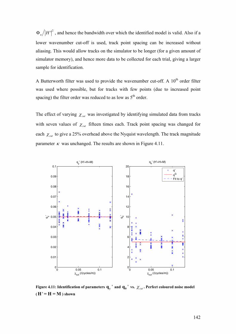
142
2'u HΦ , and hence the bandwidth over which the identified model is valid. Also if a
lower wavenumber cut-off is used, track point spacing can be increased without
aliasing. This would allow tracks on the simulator to be longer (for a given amount of
simulator memory), and hence more data to be collected for each trial, giving a larger
sample for identification.
A Butterworth filter was used to provide the wavenumber cut-off. A 10th order filter
was used where possible, but for tracks with few points (due to increased point
spacing) the filter order was reduced to as low as 5th order.
The effect of varying cutχ was investigated by identifying simulated data from tracks
with seven values of cutχ fifteen times each. Track point spacing was changed for
each cutχ to give a 25% overhead above the Nyquist wavelength. The track magnitude
parameter κ was unchanged. The results are shown in Figure 4.11.
0 0.05 0.10
0.01
0.02
0.03
0.04
0.05
0.06
0.07
0.08
0.09
0.1
χcut
(/(cycles/m))
q y′
qy′ (H′=H=M)
0 0.05 0.10
2
4
6
8
10
12
14
16
18
20
χcut
(/(cycles/m))
q θ′
qθ′ (H′=H=M)
q′
qG
Fit to q′
Figure 4.11: Identification of parameters 'yq and 'θq vs. cutχ . Perfect coloured noise model
( 'H = H = M ) shown

143
The results show little bias in 'yq or 'qθ as would be expected for a perfect noise
model. Some bias is evident in 'qθ for 0.025cutχ < cycles/m, but this seems largely
due to a single outlier for 0.005cutχ = cycles/m.
The results do show increased variance for both 'yq and 'qθ below
0.025cutχ = cycles/m. It is helpful to view this result in terms of cut-off wavelength
( 1cut cutL χ= ) relative to the driver’s preview length ( prevL ). For this model ( IG ), at
20m/s 50prevL m≈ (see chapter 3 section 3.3). If cutL is significantly longer than
prevL , little information can be gained about the shape of the preview, so identification
may be degraded. Evidence of this is seen in the increased variance of { }', 'yq qθ for
0.025cutχ < cycles/m ( 40cutL m> ).
Conversely if cutL is significantly shorter than the preview, little additional benefit
will result from increasing cutχ . Evidence of this is visible for 0.05cutχ >
( 20cutL m< ) where variance of 'yq and 'qθ does not decrease any further than that at
0.075cutχ = . In fact, it seems from these results that the variance of 'qθ for
0.075cutχ > may increase slightly, but it is unclear why this should be the case based
on the previous argument.
During simulator experiments, a track filter with wavenumber cut-off at 0.1cutχ =
cycles/m was used. This would not seem to have the least { }', 'yq qθ variance based on
these results, but for real tests the perfect noise model H is not available, and 'H
must be identified from data. In this case it is beneficial to use a track input with as
broad-band an excitation as possible to increase the signal to noise ratio for
identification of 'G in the frequency range of interest, and therefore reduce the
likelihood of bias. A wavenumber cut-off of 0.1cutχ = cycles/m implies a Nyquist
point spacing of 5 m . The track point spacing was 4m, which gave only 25% over-
head from the track Nyquist spacing, but the filter cut-off was sufficiently steep to
prevent aliasing. Tracks were tested in the simulator and found to be sufficiently
smooth for drivers to follow.

144
4.2.3 Track speed
The identification algorithm must be reliable for a range of vehicle speeds (U ) to be
useful for the experiments on drivers. Changing U will alter two aspects of the closed
loop driver-vehicle system. Firstly, the frequencies associated with a given road
wavelength input will increase as U increases, so the input ( )u ωΦ will gain
additional high frequency content. This is equivalent to changing the cut-off
wavenumber cutχ as discussed in the previous section. Secondly the LQR controller
will alter as seen in chapter 3, most notably in terms of preview distance, but also its
state gains and preview gain ‘shape’.
Identification was carried out twenty times for each of five speeds. The speeds
correspond to those used in simulator tests in chapter 5 (as shown in Table 5.1 p181).
Results are shown in Figure 4.12.
20 30 40 50 600
0.01
0.02
0.03
0.04
0.05
0.06
0.07
0.08
0.09
0.1
Vehicle speed U /(m/s)
q y′
qy′ (H′=H=M)
q′
qG
Fit to q′
20 30 40 50 600
1
2
3
4
5
6
7
8
9
10
Vehicle speed U /(m/s)
q θ′
qθ′ (H′=H=M)
Figure 4.12: Identification of parameters 'yq and 'θq vs. track speed. Perfect coloured noise
model ( 'H = H = M ) shown

145
The best fit line to the results seem to show a uniform 6% overestimation of 'yq , and
10% underestimation of 'qθ . However, only the results at 30 m/s show any visible
bias, and are probably the major cause of the best-fit lines’ offsets. The fact that this
bias at 30 m/s is not shown at other speeds seems to suggest that the result may be due
to a few outliers, and therefore not of major concern.
Significantly there seems to be little change in either bias or variance with speed U .
The identification procedure should therefore be suitable for all speeds used in
simulator testing, provided an accurate noise model can be identified. The effect of
speed on identification of each model ( IG to VIIIG ) with identified (rather than
perfect) noise models is examined in section 4.2.5.3.
4.2.4 Noise model accuracy
During identification using real driver data, the perfect noise model is not available,
and must be identified using the ARMAX method described in section 4.1.4.2.
Identification of { }', 'yq qθ is improved by an accurate noise model as shown in
equation (4.14), so it is desirable to ensure accuracy of the noise model.
Higher order ( )A q and ( )C q in the noise model '( )H q give the opportunity for the
model to be more accurate. However, fitting a noise model that is too high an order
may be detrimental because the model would tend to fit to features of the sampled
dataset, rather than reflecting the ensemble from which the dataset is taken. This
possibility is investigated in the following sections.
Section 4.2.4.1 shows the effect of model order on the accuracy of the noise model
( 'H ). Section 4.2.4.2 then shows how model order affects identification of the driver
model.

146
4.2.4.1 Effect of model order on frequency domain fit.
Models of different orders were fitted to steer angle prediction error data ( )tυ from
one track. Nine model orders were fitted. These model orders are listed in the caption
of the figure, and as titles to the subfigures in Figure 4.13, denoted as [Numerator
order/Denominator order], i.e. [order of ( )C q /order of ( )A q ]. They range from zero
order (D.C. gain), to very high order ([20/20]), and include the order [2/2] required to
express the real noise model ( H M= ). Figure 4.13 shows each model (in blue) fitted
to the spectral density of the same error data (υ ) (in magenta) on axes of PSD(υ ) vs.
frequency.
Figure 4.13: Fitting of noise model with increasing model order. o20dB = 1 /Hz . Model orders
[num/den] [0/0 , 0/1 , 0/2 , 1/2 , 2/2 , 5/5 , 5/10 , 10/5 , 20/20]. *H.H shown in blue.
Both the DC gain ([0/0]) and the single pole ([0/1]) noise models are not able to fit the
noise PSD well, and would lead to identification bias. The bias caused by these noise
−50
0
50
100
PS
D(υ
) (
/dB
)
Filter: [0/0]
−50
0
50
100Filter: [0/1]
−50
0
50
100Filter: [0/2]
−50
0
50
100
PS
D(υ
) (
/dB
)
Filter: [1/2]
−50
0
50
100Filter: [2/2]
−50
0
50
100Filter: [5/5]
10−1
100
101
−50
0
50
100
PS
D(υ
) (
/dB
)
Frequency (/Hz)
Filter: [5/10]
10−1
100
101
−50
0
50
100
Frequency (/Hz)
Filter: [10/5]
10−1
100
101
−50
0
50
100
Frequency (/Hz)
Filter: [20/20]
PSD pointARMAX fit
147
model inaccuracies is shown in the next section. All other models have two or more
poles, and fit the data similarly well, differing only in detail. Having sufficient poles
therefore seems to be the most important factor in fitting of the model.
The two-pole, two-zero model ([2/2]) is the correct order for the noise used, and
appears to fit the data better than any other model, but there is still mismatch at low
frequency. This highlights the fact that the data being fitted is only a sample of a
random process, so may not represent the whole ensemble, which the noise model is
intended to represent.
The noise models with too few zeros ([0/2], and [1/2]) have different gain from the
[2/2] noise model between 5 and 10 Hz and between 0.5 and 1 Hz, but similar gain
from 1 to 5 Hz. Increasing the number of poles and zeros to [5/5] does not seem to be
detrimental to the fit, but increasing this to [20/20] causes ‘spikes’ to appear in the
fitted PSD. This could be caused by improperly cancelled poles and zeros, or by the
model fitting to features that are a facet of this particular data sample. If this is the
case the higher order noise models would not be a good representation of the whole
ensemble, and a lower order model would help to alleviate this tendency.
4.2.4.2 Effect of model order on identification bias:
The important test for the efficacy of noise model fit is to see how it affects
identification bias. The parameters identified by each of the model orders in the
previous section are shown on axes of 'yq vs. 'qθ in Figure 4.14. The identification
domain was restricted to { } { }, 0 :10,0 : 0.1yq qθ = , so that any outliers show up as
points on the boundary of the axes.
A zero order model ([0/0] i.e. ' 1H = ) should give significant bias, as was shown in
section 4.2.1.1, and it might be expected that bias would reduce as model order was
increased. However, it is important to establish whether there is an optimal model
order, i.e. whether too high a model order causes inaccuracy.

148
Figure 4.14: Identified model parameters 'yq and 'θq with increasing noise model order. Model orders [num/den] [0/0 , 0/1 , 0/2 , 1/2 , 2/2 , 5/5 , 5/10 , 10/5 , 20/20]
The results show that significant bias is indeed present in the two lowest order cases
([0/0] and [0/1]), where noise model fit was poor. For the next two orders ([0/2] and
[2/2]) some bias towards underestimating 'qθ is evident, but for [2/2] identification
has little bias. However, as order is increased above [2/2] (that necessary to express
the real noise model) outliers begin to appear at the edge of the domain, and become
more common as noise model order is increased.
It seems from these results that over-specifying the noise model can be detrimental to
the bias and variance of the identification. It will therefore be important to select a
model order that is no greater than needed to express the noise spectrum observed
0
5
10q θ′
Filter: [0/0]
(qyG,qθ
G)
(qy′,qθ′)
0
5
10Filter: [0/1]
0
5
10Filter: [0/2]
0
5
10
q θ′
Filter: [1/2]
0
5
10Filter: [2/2]
0
5
10Filter: [5/5]
0 0.05 0.10
5
10
qy′
q θ′
Filter: [5/10]
0 0.05 0.10
5
10
qy′
Filter: [10/5]
0 0.05 0.10
5
10
qy′
Filter: [20/20]

149
during experiments. An over-complicated noise model should be evident from the
presence of outliers in ( )', 'yq qθ .
4.2.5 Time delay in loop
Incorrectly identified delay could be a source of bias. In this section time delay
identification with a perfect noise model ( 'H M= ) is investigated. First the effect of
incorrect identification of delay τ is illustrated in section 4.2.5.1, then the
performance of the time delay identification procedure is demonstrated in section
4.2.5.2. Identification with an identified noise model 'H is covered in the section
4.2.5.3.
4.2.5.1 Effect of incorrectly identified delay on bias
Figure 4.19 shows the model IG with driver delay Gτ included. The effect of
incorrect delay identification on bias was explored by fixing ' 0.2τ = s (identified
delay in equation (4.16)). The actual delay ( Gτ ) present in the driver was then varied
from 0 to 0.3 seconds. For 0.3Gτ > s the closed loop model was unstable. 'yq and
'qθ were identified for twenty trials at each Gτ value, and are shown in Figure 4.15.

150
0 0.1 0.2 0.30
0.01
0.02
0.03
0.04
0.05
0.06
0.07
0.08
0.09
0.1
τG (/s)
q y′
qy′ (H′=H=M)
q′
qG
0 0.1 0.2 0.30
1
2
3
4
5
6
7
8
9
10
τG (/s)
q θ′
qθ′ (H′=H=M)
Figure 4.15: 'yq and 'θq vs. Gτ . 'τ = 0.2 seconds for all trials
Figure 4.15 shows that there is little bias when ' 0.2 secsGτ τ= = (i.e. the real delay
matches the identified delay), but significant underestimation of both 'yq and 'qθ
when 0.2Gτ < s (real delay is less than the identified delay). When 0.2 secsGτ >
(real delay exceeds the identified delay), the pattern of bias is less clear, but is non-
zero for both 'yq and 'qθ . It is clear that finding the correct delay is very important
for avoiding bias.
4.2.5.2 Identification of delay using identification procedure
To demonstrate whether the algorithm correctly identifies delay, identification of
( )', ', 'yq qθ τ was attempted on models with a range of Gτ from 0 to 0.3 seconds using
the full procedure of section 4.1.4.3. Results for identification of 'τ are shown in
Figure 4.16. 'τ is discrete, so the points are artificially blurred to show number of
identifications at each delay point, and the number of points is shown in brackets. A

151
least squares fit line to the identified delay is shown by the blue dashed line, and
perfect delay identification is shown in red.
0 0.05 0.1 0.15 0.2 0.25 0.3 0.350
0.05
0.1
0.15
0.2
0.25
0.3
τG (/s)
τ′ (
/s)
τ′Perfect identification (τ′=τG)LSq fit line
(19)
(19)
(20)
(20)
(20)
(20)
(20)
(1)
(1)
Figure 4.16: identified delay 'τ (/secs) vs. actual model delay Gτ (/secs). 'H = H = M
The result shows perfect identification in all but two cases out of 140 trials. Note,
however, that this is for perfect noise model case ( 'H H M= = ), and may not be as
good with an identified noise model ( 'H H≠ ). Results for identification of 'yq and
'qθ for the same trial are shown in Figure 4.17.

152
0 0.1 0.2 0.30
0.01
0.02
0.03
0.04
0.05
0.06
0.07
0.08
0.09
0.1
τG (/s)
q y′
qy′ (H′=H=M)
q′
qG
Fit to q′
0 0.1 0.2 0.30
1
2
3
4
5
6
7
8
9
10
τG (/s)
q θ′
qθ′ (H′=H=M)
Figure 4.17: Identified parameters ' 'y θ(q ,q ) vs. real model delay Gτ (/s) with 'H = H = M
Best fit lines to these results show little systematic bias in 'yq and little dependence
on Gτ . 'qθ seems to show increased bias with increased Gτ , but this is mainly due to
outliers for 0.2Gτ = , because of the large variance in 'qθ . Delay in real drivers is
likely to be close to 0.2 seconds [36, 39], so if a perfect noise model could be found,
the bias in { }', 'yq qθ would be acceptable.
Bias due to identification of 'τ becomes more complicated when 'H has to be
identified, because the two identifications are interdependent. However, the iterative
computation of noise model and model optimisation as explained in section 4.1.4.3
should minimise any resulting bias. Identification of ( )', ', 'yq qθ τ with an identified
'H is covered in the next section (4.2.5.3).

153
4.2.5.3 Identification of time delay with an identified noise model
Figure 4.16 showed that near perfect identification of 'τ was possible with 'H H= .
However, when identifying real data the noise model has to be identified, and the
identification of 'τ may be degraded as a result. To test this, one iteration of the
algorithm from section 4.1.4.3 was carried out to identify ( )', ', 'yq qθ τ for a range of
00 ' 0.3τ≤ ≤ (i.e. the delay assumed when fitting 1'H ). The identification was tried at
three Gτ values (0, 0.1, 0.2 secs), and three driver noise levels ( ) [1 ,5 ,10 ]ηΞ =
giving nine combinations shown on the subplots of Figure 4.18. Each subplot shows
1'τ vs. 0'τ for 30 trials.
For successful iteration 'τ must approach Gτ for successive iterations (i.e. 1' 'i iτ τ −<
for 1' Giτ τ− > , and 1' 'i iτ τ −> for 1' G
iτ τ− < ). This region is that bounded by the solid
and the dashed lines in each of the subplots of Figure 4.18. The algorithm will not
iterate toward a correct 'τ if 1' 'i iτ τ −= for ' Giτ τ≠ , so any identifications on the
dashed line 1 0' 'τ τ= indicate that 'τ , and hence 'yq and 'qθ (see section 4.2.5.1) will
be incorrect.
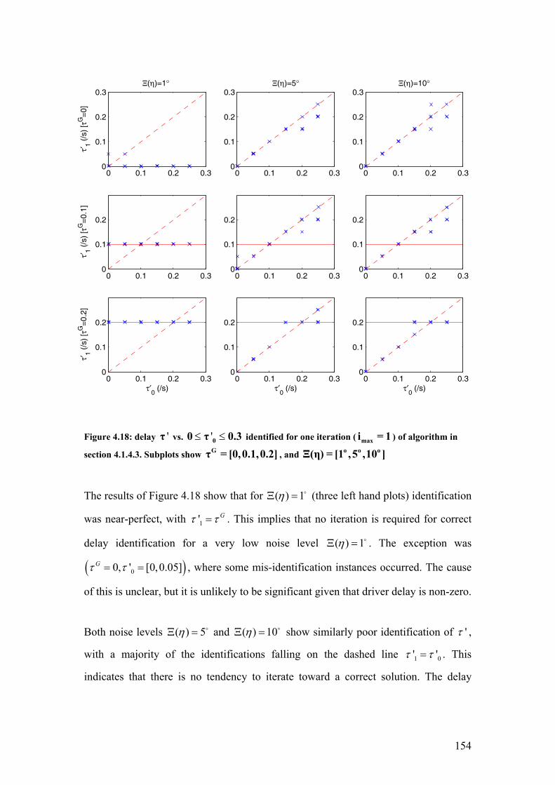
154
Figure 4.18: delay 'τ vs. '≤ ≤00 τ 0.3 identified for one iteration ( maxi = 1 ) of algorithm in
section 4.1.4.3. Subplots show Gτ = [0,0.1,0.2] , and o o oΞ(η) = [1 ,5 ,10 ]
The results of Figure 4.18 show that for ( ) 1ηΞ = (three left hand plots) identification
was near-perfect, with 1'Gτ τ= . This implies that no iteration is required for correct
delay identification for a very low noise level ( ) 1ηΞ = . The exception was
( )00, ' [0,0.05]Gτ τ= = , where some mis-identification instances occurred. The cause
of this is unclear, but it is unlikely to be significant given that driver delay is non-zero.
Both noise levels ( ) 5ηΞ = and ( ) 10ηΞ = show similarly poor identification of 'τ ,
with a majority of the identifications falling on the dashed line 1 0' 'τ τ= . This
indicates that there is no tendency to iterate toward a correct solution. The delay
0 0.1 0.2 0.30
0.1
0.2
0.3Ξ(η)=1°
τ′1 (
/s)
[τG
=0]
0 0.1 0.2 0.30
0.1
0.2
0.3Ξ(η)=5°
0 0.1 0.2 0.30
0.1
0.2
0.3Ξ(η)=10°
0 0.1 0.2 0.30
0.1
0.2
τ′1 (
/s)
[τG
=0.
1]
0 0.1 0.2 0.30
0.1
0.2
0 0.1 0.2 0.30
0.1
0.2
0 0.1 0.2 0.30
0.1
0.2
τ′0 (/s)
τ′1 (
/s)
[τG
=0.
2]
0 0.1 0.2 0.30
0.1
0.2
τ′0 (/s)
0 0.1 0.2 0.30
0.1
0.2
τ′0 (/s)
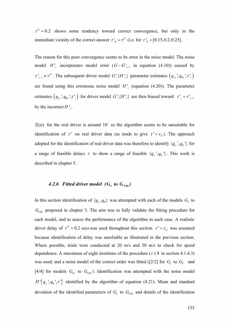
155
0.2Gτ = shows some tendency toward correct convergence, but only in the
immediate vicinity of the correct answer 0'Gτ τ= (i.e. for 0' [0.15,0.2,0.25]τ = .
The reason for this poor convergence seems to be error in the noise model. The noise
model 'iH incorporates model error ( 1'iG G −− in equation (4.10)) caused by
1' Giτ τ− ≠ . The subsequent driver model ' { ' }i iG H parameter estimates ( )', ', 'yi i iq qθ τ
are found using this erroneous noise model 'iH (equation (4.20)). The parameter
estimates ( )', ', 'yi i iq qθ τ for driver model ' { ' }i iG H are then biased toward 1' 'i iτ τ −=
by the incorrect 'iH .
( )ηΞ for the real driver is around 10 so the algorithm seems to be unsuitable for
identification of 'τ on real driver data (as tends to give 0'τ τ= ). The approach
adopted for the identification of real driver data was therefore to identify { ', '}yq qθ for
a range of feasible delays τ to show a range of feasible { ', '}yq qθ . This work is
described in chapter 5.
4.2.6 Fitted driver model ( IG to VIIIG )
In this section identification of { , }yq qθ was attempted with each of the models IG to
VIIIG proposed in chapter 3. The aim was to fully validate the fitting procedure for
each model, and to assess the performance of the algorithm in each case. A realistic
driver delay of 0.2 secsGτ = was used throughout this section. ' Gτ τ= was assumed
because identification of delay was unreliable as illustrated in the previous section.
Where possible, trials were conducted at 20 m/s and 50 m/s to check for speed
dependence. A maximum of eight iterations of the procedure ( 8i ≤ in section 4.1.4.3)
was used, and a noise model of the correct order was fitted ([2/2] for IG to VG and
[4/4] for models VIG to VIIIG ). Identification was attempted with the noise model
{ }' ', ', 'yH q qθ τ identified by the algorithm of equation (4.21). Mean and standard
deviation of the identified parameters of IG to VIIIG and details of the identification
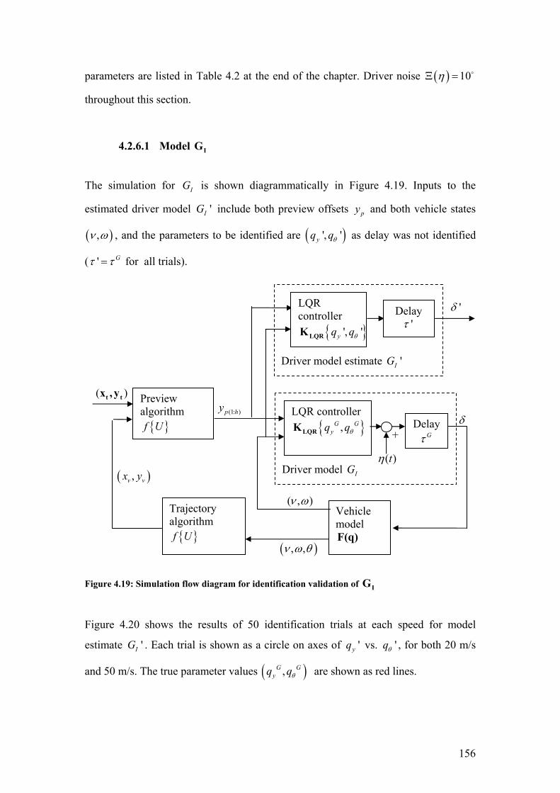
156
parameters are listed in Table 4.2 at the end of the chapter. Driver noise ( ) 10ηΞ =
throughout this section.
4.2.6.1 Model IG
The simulation for IG is shown diagrammatically in Figure 4.19. Inputs to the
estimated driver model 'IG include both preview offsets py and both vehicle states
( ),ν ω , and the parameters to be identified are ( )', 'yq qθ as delay was not identified
( ' Gτ τ= for all trials).
Figure 4.19: Simulation flow diagram for identification validation of IG
Figure 4.20 shows the results of 50 identification trials at each speed for model
estimate 'IG . Each trial is shown as a circle on axes of 'yq vs. 'qθ , for both 20 m/s
and 50 m/s. The true parameter values ( ),G Gyq qθ are shown as red lines.
Driver model IG ( ),v vx y
(1: )p hy δ
Vehicle model F(q)
Trajectory algorithm { }f U
( ), ,ν ω θ
( , )ν ω
LQR controller { },G G
yq qθLQRK
Driver model estimate 'IG
LQR controller
{ }', 'yq qθLQRK
'δ
Delay Gτ
( )tη
+
Delay 'τ
Preview algorithm { }f U
( )t tx , y

157
0 0.02 0.04 0.06 0.08 0.10
1
2
3
4
5
6
7
8
9
10
qy′
q θ′
ID of (qy′,qθ′) with U=20 m/s
(qyG,qθ
G)
(qy′,qθ′)
0 0.02 0.04 0.06 0.08 0.10
1
2
3
4
5
6
7
8
9
10
qy′
q θ′
ID of (qy′,qθ′) with U=50 m/s
(qyG,qθ
G)
(qy′,qθ′)
Figure 4.20: Identification of IG at 20 m/s and 50 m/s with ' = Gτ τ = 0.2 secs , using
{ }' ' ' 'y θH q ,q , τ (noise model identified using equation (4.21))
Bias in the parameter estimates was measured using the percentage error in the mean
of the identified parameters as in equation (4.26). The variance of the identified
parameters was measured using the standard deviation of the identified parameters as
a percentage of the true parameter value, as shown in equation (4.27).
( ) ( )( ') ( ')
( ', ') 100 ,G G
y yerr y G G
y
q q q qq q
q qθ θ
θθ
µ µµ
− − =
(4.26)
( ') ( ')( ', ') 100 ,y
err y G Gy
q qq qq q
θθ
θ
σ σσ
=
(4.27)
At 20 m/s, bias is small for both parameters ( ', ') ( 2.2, 4.6)%err yq qθµ = − − . Standard
deviation was three times larger for 'qθ than 'yq with ( ', ') (12.8,33.8)%err yq qθσ = .
This result is consistent with that observed for the perfect noise model case. The
larger bias for 'qθ is consistent with its larger variance given the limited sample size.

158
At 50 m/s, slightly less variance was found ( ', ') (10.8,32.1)%err yq qθσ = , giving even
lower bias ( ', ') ( 1.0, 0.4)%err yq qθµ = − − . There seems to be little dependence of the
identification on speed. Neither of the speeds show a correlation between ( ')yqµ and
( ')qθµ so bias of 'yq and 'qθ is independent.
4.2.6.2 Model IIG
The same procedure was used to validate identification of 'IIG . Figure 4.21 shows the
simulation for IIG where the only input to IIG is the preview py . 50 trials
identifying 'yq and 'qθ were carried out at 20 m/s only. Figure 4.22 shows the
identification results for this model.
Figure 4.21: Simulation flow diagram for identification validation of IIG
Driver model IIG
LQR controller { },G G
yq qθLQRK
( ),v vx y
(1: )p hy
Vehicle model F(q) ( ), ,ν ω θ
Driver model estimate 'IIG
LQR controller
{ }', 'yq qθLQRK
Delay 'τ
'δ
( )tη
δ Delay Gτ
Trajectory algorithm { }f U
Preview algorithm { }f U
( )t tx , y
+

159
0 0.01 0.02 0.03 0.04 0.05 0.06 0.07 0.08 0.09 0.10
1
2
3
4
5
6
7
8
9
10
qy′
q θ′
ID of (qy′,qθ′) with U=20 m/s
(qyG,qθ
G)
(qy′,qθ′)
Figure 4.22:Identification of IIG with Gτ = 0.2 secs , using { }' ' ' 'y θH q ,q , τ (noise model
identified using equation (4.21))
Bias is less than for IG for both parameters ( ', ') ( 1.0,0.4)%err yq qθµ = − and variance
is similar to that for IG with ( ', ') (11.4,29.5)%err yq qθσ = .
It was not possible to validate the model at 50 m/s because with delay present, the
driver-vehicle system is unstable with these ( , )G Gyq qθ values. This does not mean
that the model is invalid at high speed, as a driver might use other ( , )G Gyq qθ .
However, if ( ', ') (0.05,5)yq qθ = were identified from real data at high speed the
results would be suspicious, as such a controller is known to be unstable even without
noise present.

160
4.2.6.3 Model IIIG
The simulation carried out for identification of 'IIIG is shown in Figure 4.23. Driver
model inputs are now py and ω , and again ( ', ')yq qθ must be identified. Results for
identification at 20m/s and 50m/s are shown in Figure 4.24.
Figure 4.23: Simulation flow diagram for identification validation of IIIG
Driver model IIIG
( ),v vx y
(1: )p hy
Vehicle model F(q)
( ), ,ν ω θ
( )ω
LQR controller { },G G
yq qθLQRK
Driver model estimate 'IIIG
LQR controller
{ }', 'yq qθLQRK
Delay 'τ
'δ
δ Delay Gτ
( )tη
Trajectory algorithm { }f U
Preview algorithm { }f U
( )t tx , y
+
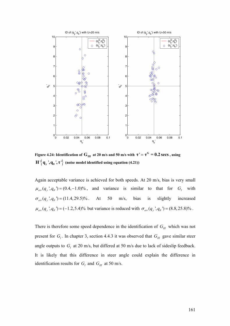
161
0 0.02 0.04 0.06 0.08 0.10
1
2
3
4
5
6
7
8
9
10
qy′
q θ′
ID of (qy′,qθ′) with U=20 m/s
(qyG,qθ
G)
(qy′,qθ′)
0 0.02 0.04 0.06 0.08 0.10
1
2
3
4
5
6
7
8
9
10
qy′
q θ′
ID of (qy′,qθ′) with U=50 m/s
(qyG,qθ
G)
(qy′,qθ′)
Figure 4.24: Identification of IIIG at 20 m/s and 50 m/s with ' = Gτ τ = 0.2 secs , using
{ }' ' ' 'y θH q ,q , τ (noise model identified using equation (4.21))
Again acceptable variance is achieved for both speeds. At 20 m/s, bias is very small
( ', ') (0.4, 1.0)%err yq qθµ = − , and variance is similar to that for IG with
( ', ') (11.4,29.5)%err yq qθσ = . At 50 m/s, bias is slightly increased
( ', ') ( 1.2,5.4)%err yq qθµ = − but variance is reduced with ( ', ') (8.8, 25.8)%err yq qθσ = .
There is therefore some speed dependence in the identification of IIIG which was not
present for IG . In chapter 3, section 4.4.3 it was observed that IIIG gave similar steer
angle outputs to IG at 20 m/s, but differed at 50 m/s due to lack of sideslip feedback.
It is likely that this difference in steer angle could explain the difference in
identification results for IG and IIIG at 50 m/s.

162
4.2.6.4 Model IVG
Figure 4.25 shows the simulation schematic for IVG . This model involves feedback of
the steer angle delay states 1,...,dNδ δ− as well as py and ( , )ν ω .
Identification of dN was attempted, but was unsuccessful. It was shown in chapter 3
section 4.4.6 that steer angle δ for IG and { }4IV dG N = are almost identical. Noting
also that { }0I IV dG G N= = , this implies that the steer angle time histories
{ }( 0 )IV dG Nδ = and { }( 4 )IV dG Nδ = are almost identical. This implies that 'dN will
have very little effect on 'δ . This fact makes identification of 'dN poor because the
prediction error ε (where ( )1' 'Hε δ δ−= − ) will not be affected by 'dN , and hence
the optimisation routine fminsearch cannot converge to the correct 'dN value. For
this reason ' 4d dN N= = for all identifications in this section.
As for previous models, the parameters to be identified for IVG are ( ', ')yq qθ , with
' 0.2Gτ τ= = s. Figure 4.26 shows the results of 50 identifications for 20 m/s and 50
m/s.

163
Figure 4.25: Simulation flow diagram for identification validation of IVG
Equation 3.22
δ Driver Model IVG
(1: )p ny Trajectory algorithm { }f U
( ), ,ν ω θ
Ndδ
Vehicle model F(q)
Delay ( ) ( )Gk k Ndδ δ= −
δ ( ),ν ω
Driver Model 'IVG
LQR controller { }', ', 'y dq q NθLQRK
Ndδ Delay ( ) ( ')dk k Nδ δ= −
'δ Delay 'τ
Delay Gτ
( )tη
( )1,...,Ndδ δ−
LQR controller { }, ,G G G
yq q NdθLQRK
Preview algorithm { }f U
( )t tx , y

164
0 0.02 0.04 0.06 0.08 0.10
1
2
3
4
5
6
7
8
9
10
qy′
q θ′
ID of (qy′,qθ′) with U=20 m/s
(qyG,qθ
G)
(qy′,qθ′)
0 0.02 0.04 0.06 0.08 0.10
1
2
3
4
5
6
7
8
9
10
qy′
q θ′
ID of (qy′,qθ′) with U=50 m/s
(qyG,qθ
G)
(qy′,qθ′)
Figure 4.26: Identification of IVG at 20 m/s and 50 m/s with ' = Gτ τ = 0.2 secs ,
' =d dN N = 4 , using { }' ' ' 'y θH q ,q , τ (noise model identified using equation (4.21))
At 20 m/s, both bias and variance are slightly larger than those of IG with
( ', ') (1.0,6.1)%err yq qθµ = and ( ', ') (14.0,36.7)%err yq qθσ = . At 50 m/s, both bias and
variance are similar to IG with ( ', ') ( 1.2, 2.0)%err yq qθµ = − − and
( ', ') (11.8,32.3)%err yq qθσ = . The similarity of bias and variance at both speeds is
consistent with the similarity in steer angleδ for IG and IVG seen in section 3.4.5.

165
4.2.6.5 Model VG
The simulation carried out for identification of 'VG is shown in Figure 4.27. For VG
the parameters ( )', ', 'y nq qθ ω were identified, but only 30 trials were carried out, as
the identification was much slower with a three dimensional parameter space to
search. 'ξ was not identified, but set to ' 0.707Gξ ξ= = . A value of 1 HzGnω = was
used. Only results for identifications at 20 m/s are shown in Figure 4.28 because VG
is unstable at 50 m/sU = with the parameter values chosen.
Figure 4.27: Simulation flow diagram for identification validation of VG
Driver model VG
(1: )p hy Preview algorithm { }f U
Trajectory algorithm { }f U
( ), ,ν ω θ
LQR controller { },G G
yq qθLQRKnmsδ
Equation (3.37)
Vehicle model F(q)
Neuromuscular system filter { },G G
nω ξN
outδ ( ),ν ω
Driver model estimate 'VG
LQR controller { }', 'yq qθLQRK
Neuromuscular system filter { }', G
nω ξN Delay
'τ
'nmsδ 'outδ
Delay Gτ
( )tη
outδ
( )t tx , y
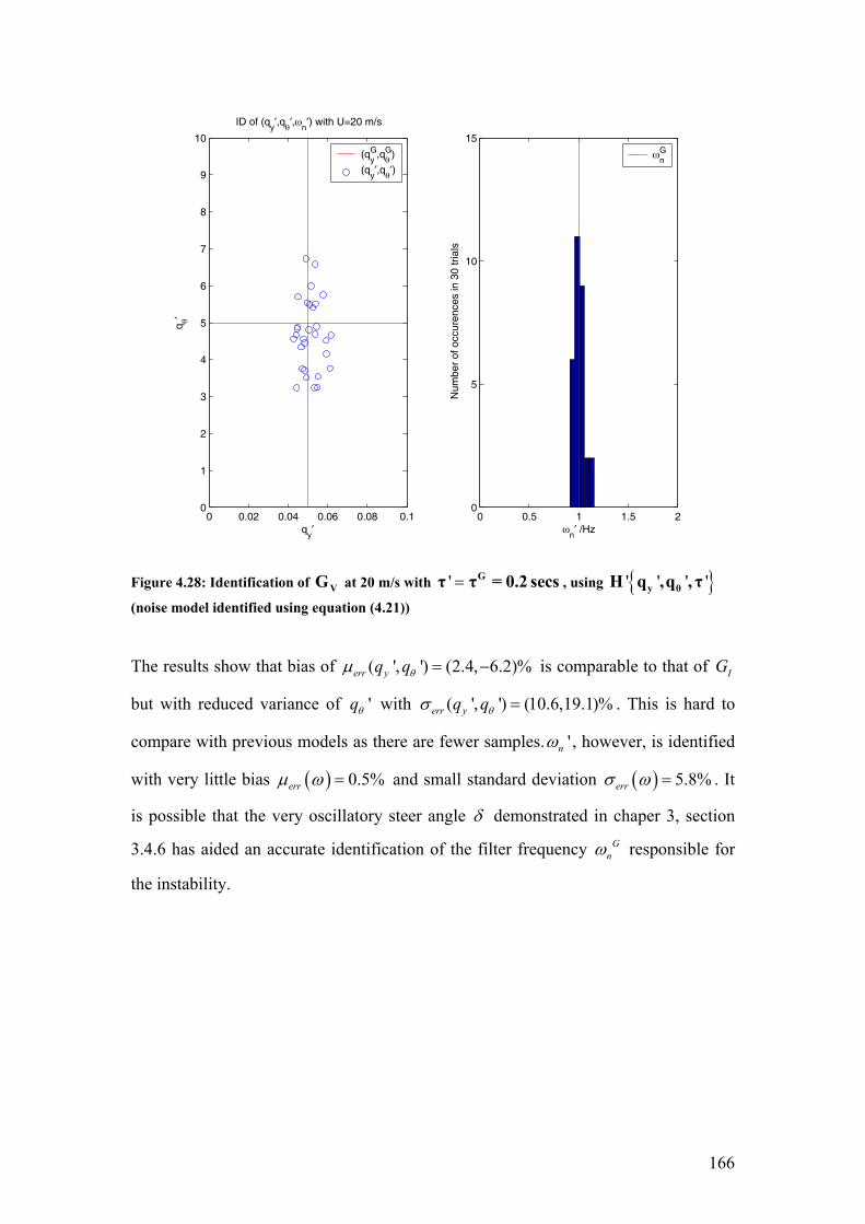
166
0 0.02 0.04 0.06 0.08 0.10
1
2
3
4
5
6
7
8
9
10
qy′
q θ′
ID of (qy′,qθ′,ωn
′) with U=20 m/s
(qyG,qθ
G)
(qy′,qθ′)
0 0.5 1 1.5 20
5
10
15
ωn′ /Hz
Num
ber
of o
ccur
ence
s in
30
tria
ls
ωnG
Figure 4.28: Identification of VG at 20 m/s with ' = Gτ τ = 0.2 secs , using { }' ' ' 'y θH q ,q , τ
(noise model identified using equation (4.21))
The results show that bias of ( ', ') (2.4, 6.2)%err yq qθµ = − is comparable to that of IG
but with reduced variance of 'qθ with ( ', ') (10.6,19.1)%err yq qθσ = . This is hard to
compare with previous models as there are fewer samples. 'nω , however, is identified
with very little bias ( ) 0.5%errµ ω = and small standard deviation ( ) 5.8%errσ ω = . It
is possible that the very oscillatory steer angle δ demonstrated in chaper 3, section
3.4.6 has aided an accurate identification of the filter frequency Gnω responsible for
the instability.

167
4.2.6.6 Model VIG
The simulation for identification of 'VIG is shown in
Figure 4.29. VIG features an NMS filter but also uses the ( , )nω ξ parameters in the
derivation of the LQR controller gains. Initially, identification of all parameters
( )', ', ', 'y nq qθ ω ξ was attempted and is shown for 20 m/sU = in Figure 4.30 and
50 m/sU = in Figure 4.31 on axes of ( )', 'yq qθ and ( )', 'nω ξ . Again ' 0.2Gτ τ= = s,
1 HzGnω = , and 0.45Gξ = as used in chapter 3. Only thirty trials were conducted at
each speed due to much slower convergence of the fminsearch algorithm with a four
dimensional parameter space to search.
Figure 4.29: Simulation flow diagram for identification validation of , ,VI VII VIIIG G G
Driver model , ,VI VII VIIIG G G
(1: )p hy Preview algorithm { },f Ut tx , y
Trajectory algorithm { }f U
( ), ,ν ω θ
LQR controller { }, , ,G G G G
y nq qθ ω ξLQRKnmsδ
Equation (3.37)
Vehicle model F(q)
Neuromuscular system filter { },G G
nω ξN
outδ ( ),ν ω
( ),δ δ
Driver model estimate ', ', 'VI VII VIIIG G G
LQR controller { }', ', ', 'y nq qθ ω ξLQRK
Neuromuscular system filter { }', 'nω ξN
Delay 'τ
'nmsδ 'outδ
Delay Gτ
( )tη
outδ

168
0 0.02 0.04 0.06 0.08 0.10
1
2
3
4
5
6
7
8
9
10
qy′
q θ′
ID of (qy′,qθ′,ωn
′,ζ′) with U=20 m/s
(qyG,qθ
G)
(qy′,qθ′)
0 1 2 30
0.1
0.2
0.3
0.4
0.5
0.6
0.7
0.8
0.9
1
ωn′ /Hz
ζ n′
(ωnG,ζ
nG)
(ωn′,ζ
n′)
Figure 4.30: Identification of VIG at 20 m/s with ' = Gτ τ = 0.2 secs , using { }' ' ' 'y θH q ,q , τ
(noise model identified using equation (4.21))
At 20 m/s, although the bias of ( ', ') (3.6, 4.7)%err yq qθµ = − seems acceptable, the
standard deviation of ( ', ') (34.4,89.5)%err yq qθσ = is three times that of IG , and for
( ', ')nω ξ the variance is very large with ( ', ') (81.5,89.6)%err nσ ω ξ = . It is clear from
Figure 4.30 that a few outliers, shown artificially at the edge of the axes, are
correcting the mean. If these outliers were removed from the data set a large bias
would be evident.

169
0 0.02 0.04 0.06 0.08 0.10
1
2
3
4
5
6
7
8
9
10
qy′
q θ′
ID of (qy′,qθ′,ωn
′,ζ′) with U=50 m/s
(qyG,qθ
G)
(qy′,qθ′)
0 1 2 30
0.1
0.2
0.3
0.4
0.5
0.6
0.7
0.8
0.9
1
ωn′ /Hz
ζ n′
(ωnG,ζG)
(ωn′,ζ′)
Figure 4.31: Identification of VIG at 50 m/s with ' = Gτ τ = 0.2 secs , using { }' ' ' 'y θH q ,q , τ
(noise model identified using equation (4.21))
The results for 50 m/s show fewer outliers, and consequently lower variance than at
20 m/s for most parameters with ( ', ', ', ') (30.8,62.2,41.8,98.4)%err y nq qθσ ω ξ = .
However, this means that the means of the estimates ( ', ', ', ')err y nq qθµ ω ξ are no
longer corrected by the outliers, giving larger bias particularly for 'qθ with
( ', ', ', ') ( 9.4, 28.5,1.0,22.9)%err y nq qθµ ω ξ = − − .
The variance for identification is much greater than that of VG , and may be a result of
identifying four parameters for VIG with the same amount of information available. In
order to test this, identification was attempted for parameters ( ', ', ')y nq qθ ω with
' Gξ ξ= (model VIIG in section 4.2.6.7), then for ( ', ', ')yq qθ ξ with 'n nω ω= (model
VIIIG in section 4.2.6.8).

170
4.2.6.7 Model VIIG
VIIG is the same as VIG but only ( ', ', ')y nq qθ ω were identified, while ' Gξ ξ= . Results
for identification of parameters ( ', ', ')y nq qθ ω are shown in Figure 4.32 for 20U = m/s
and Figure 4.33 for 50U = m/s.
0 0.02 0.04 0.06 0.08 0.10
1
2
3
4
5
6
7
8
9
10
qy′
q θ′
ID of (qy′,qθ′,ωn
′) with U=20 m/s
(qyG,qθ
G)
(qy′,qθ′)
0 1 2 30
1
2
3
4
5
6
7
8
9
10
ωn′ /Hz
Num
ber
of o
ccur
ence
s in
30
tria
ls
ωnG
Figure 4.32: Identification of VIIG at 20 m/s with ' = Gτ τ = 0.2 secs , using { }' ' ' 'y θH q ,q , τ
(noise model identified using equation (4.21))
At 20 m/s, ( ', ', ') ( 3.4, 15.4, 17.1)%err y nq qθµ ω = − − − . At first this seems to be worse
than the result for VIG , however, from the figure it is clear that the identifications are
far more closely gathered around the correct value. This closer grouping is reflected in
the standard deviation ( ', ', ') (24.4,31.3,13.7)%err y nq qθσ ω = being less than half that
of VIG .
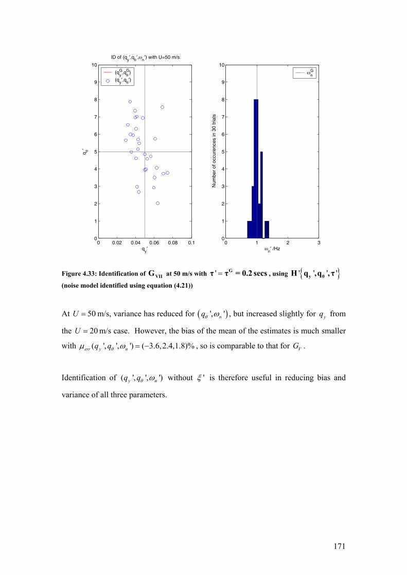
171
0 0.02 0.04 0.06 0.08 0.10
1
2
3
4
5
6
7
8
9
10
qy′
q θ′
ID of (qy′,qθ′,ωn
′) with U=50 m/s
(qyG,qθ
G)
(qy′,qθ′)
0 1 2 30
1
2
3
4
5
6
7
8
9
10
ωn′ /Hz
Num
ber
of o
ccur
ence
s in
30
tria
ls
ωnG
Figure 4.33: Identification of VIIG at 50 m/s with ' = Gτ τ = 0.2 secs , using { }' ' ' 'y θH q ,q , τ
(noise model identified using equation (4.21))
At 50U = m/s, variance has reduced for ( )', 'nqθ ω , but increased slightly for yq from
the 20U = m/s case. However, the bias of the mean of the estimates is much smaller
with ( ', ', ') ( 3.6, 2.4,1.8)%err y nq qθµ ω = − , so is comparable to that for VG .
Identification of ( ', ', ')y nq qθ ω without 'ξ is therefore useful in reducing bias and
variance of all three parameters.

172
4.2.6.8 Model VIIIG
VIIIG is the same as VIG but only ( ', ', ')yq qθ ξ are identified, with ' Gn nω ω= . Results
for identification of parameters ( ', ', ')yq qθ ξ are shown in Figure 4.34 for 20U = m/s ,
and Figure 4.35 for 50U = m/s.
0 0.02 0.04 0.06 0.08 0.10
1
2
3
4
5
6
7
8
9
10
qy′
q θ′
ID of (qy′,qθ′,ζ′) with U=20 m/s
(qyG,qθ
G)
(qy′,qθ′)
0 0.2 0.4 0.6 0.8 10
1
2
3
4
5
6
7
8
9
10
ζ′
Num
ber
of o
ccur
ence
s in
30
tria
ls
ζG
Figure 4.34: Identification of VIIIG at 20 m/s with ' = Gτ τ = 0.2 secs , using { }' ' ' 'y θH q ,q , τ
(noise model identified using equation (4.21))
At 20U = m/s variance was large for all parameters with
( ', ', ') (34.2,66.5,135.6)%err yq qθσ ξ = , this is particularly true for 'ξ meaning many
of the 30 identifications of 'ξ are outside the axes. This led to poor bias for ( )', 'yq ξ ,
with ( ', ', ') (13.6, 3.1,31.5)%err yq qθµ ξ = − .
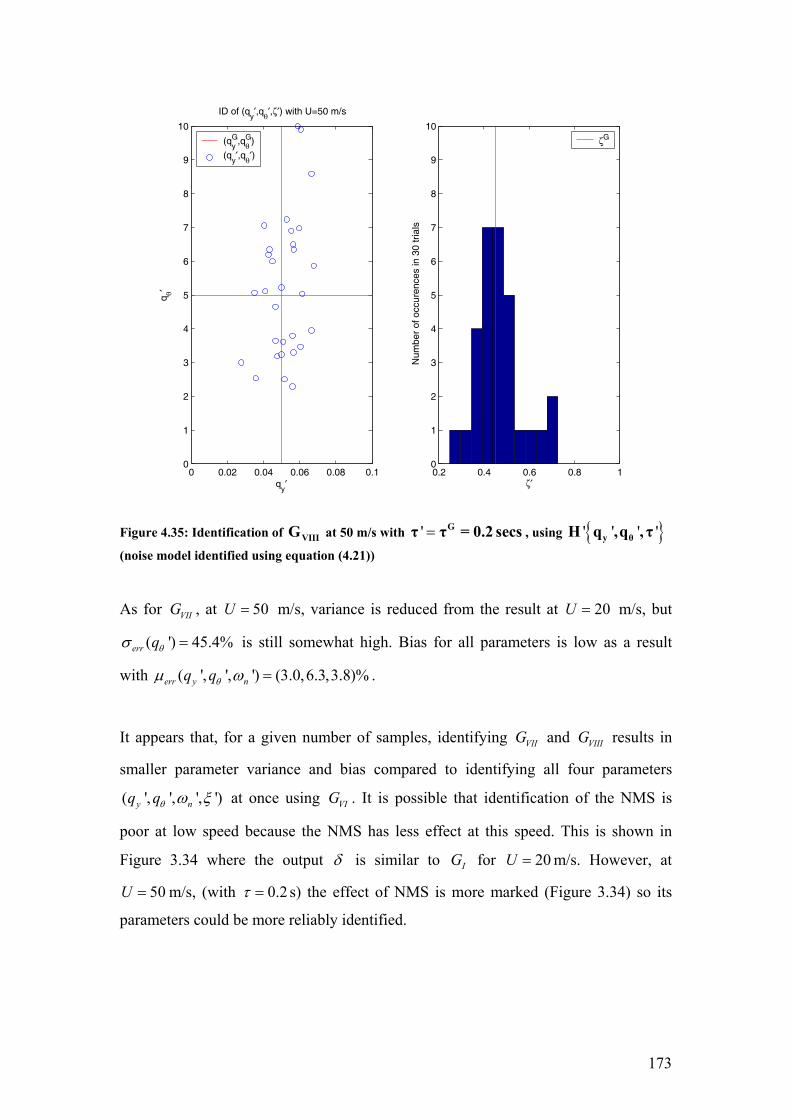
173
0 0.02 0.04 0.06 0.08 0.10
1
2
3
4
5
6
7
8
9
10
qy′
q θ′
ID of (qy′,qθ′,ζ′) with U=50 m/s
(qyG,qθ
G)
(qy′,qθ′)
0.2 0.4 0.6 0.8 10
1
2
3
4
5
6
7
8
9
10
ζ′
Num
ber
of o
ccur
ence
s in
30
tria
ls
ζG
Figure 4.35: Identification of VIIIG at 50 m/s with ' = Gτ τ = 0.2 secs , using { }' ' ' 'y θH q ,q , τ
(noise model identified using equation (4.21))
As for VIIG , at 50U = m/s, variance is reduced from the result at 20U = m/s, but
( ') 45.4%err qθσ = is still somewhat high. Bias for all parameters is low as a result
with ( ', ', ') (3.0,6.3,3.8)%err y nq qθµ ω = .
It appears that, for a given number of samples, identifying VIIG and VIIIG results in
smaller parameter variance and bias compared to identifying all four parameters
( ', ', ', ')y nq qθ ω ξ at once using VIG . It is possible that identification of the NMS is
poor at low speed because the NMS has less effect at this speed. This is shown in
Figure 3.34 where the output δ is similar to IG for 20U = m/s. However, at
50U = m/s, (with 0.2τ = s) the effect of NMS is more marked (Figure 3.34) so its
parameters could be more reliably identified.

174
4.3 Conclusions
Two possible approaches to driver identification were considered, namely the direct
and indirect methods. The direct method was chosen for the identification of real
drivers because it involved significantly less CPU time. Weighting the prediction
error υ by using a noise model reduces bias in identification of systems operating in
closed loop [47], however, a good noise model is required for bias free identification.
An iterative procedure was required to determine both the driver model and the noise
model, so such a procedure was designed for use in identifying driver model
parameters.
A validation was carried out to check that the identification procedure and the road
path excitation parameters were suitable for giving an unbiased identification of the
driver model. Validation consisted of a known controller driving a road path in closed
loop with a vehicle, followed by an identification of the model parameters
( )', ', ', 'y nq qθ ω ξ using the inputs and outputs of the known LQR controller. Bias of
identification was demonstrated when a white noise model ( ' 1H = ) was used to
identify data created using coloured driver noise ( )H M= . A perfect noise model
( 'H M= ) eliminated bias when the driver noise η was coloured using a realistic
noise filter ( H M= ).
Validation of the identification bias of ( )', 'yq qθ was carried out for a range of values
of each experiment parameter. Experiment parameter values suitable for driver
experiments were determined from this validation. It was found that the track PSD
amplitude parameter κ should be as large as possible to minimise bias and variance of
( )', 'yq qθ by increasing the signal to noise ratio. Road spectral density roll-off
gradient 2γ ≥ − gave improved variance and bias of ( )', 'yq qθ . For driver
experiments 2γ = − was used which corresponds to white noise road curvature.

175
Track wavenumber cut-off values 0.05cutχ ≥ cycles/m gave similar bias and variance
of ( )', 'yq qθ . Driver experiments were carried out using 0.1cutχ = to give good signal
to noise ratio for noise model identification. Bias and variance of ( )', 'yq qθ was not
affected systematically by vehicle speed U , so the identification procedure was
suitable for data gathered from driver experiments at different vehicle speeds. A
noise model 'H of too low an order led to identification bias, but a noise model of
too high an order was prone to outliers of ( )', 'yq qθ . The order of the noise model 'H
must therefore be just sufficient to express the noise present.
Time delay 'τ was nearly perfectly identified when a perfect noise model was used
( 'H H M= = ). However, with an identified noise model 'H , misidentification of 'τ
occurred for ( ) 5ηΞ ≥ . For a realistic driver noise level ( ( ) 10ηΞ = ), time delay did
not iterate away from its initial value ( 1 0' 'τ τ= ). Delay 'τ therefore could not be
reliably identified, and for the identification using real driver data in chapter 5 a range
of realistic driver delays is investigated.
Identification of each of the driver models IG to VIIIG was validated at 20U = m/s
and 50U = m/s with an identified noise model 'H , but with correct time delay
( ' Gτ τ= ). 'IG to 'IVG were all identified with small bias (<6.1%) for both parameters
( )', 'yq qθ . Standard deviation of 'qθ was approximately three times that of 'yq for
these models. Vehicle speed had little effect on identification bias or variance of
( )', 'yq qθ for these models.
'VG was identified with similar bias and variance of ( )', 'yq qθ to that found for 'IG .
'nω had even lower bias (0.5%) and standard deviation (<6%). 'VIG had very large
variance of 'yq and 'qθ , leading to large bias for some parameters and rendering the
model 'VIG unreliable for use in driver identification in chapter 5. 'VIIG and 'VIIIG are
more successful at identifying NMS parameters than 'VIG , giving much smaller
variance of 'yq and 'qθ . However, both have large bias of 'yq and 'qθ at 20 m/s.

176
Controller Driver noise Noise model Track input Time delay
Figure subplot Model yq qθ H ( )eΞ ( )ηΞ 'H
num den cutχ (/1/m) γ κ 0( )eδ =Ξ U Gτ 'τ 0'τ
Figure 4.5 IG 5 0.05 1 0 to 16 1 not fitted 0.05 -2 5.0E-05 11.50 20 0 ID -
Figure 4.7 1 IG 5 0.05 M 0 to 16 1 not fitted 0.05 -2 5.0E-05 11.50 20 0 0 -
Figure 4.7 2 IG 5 0.05 M 0 to 16 M not fitted 0.05 -2 5.0E-05 11.50 20 0 0 -
Figure 4.9 IG 5 0.05 M 10 M not fitted 0.05 -2 [5e-7 to 5e-5] 1 to 11.5 20 0 0 -
Figure 4.10 IG 5 0.05 M 10 M not fitted 0.05 [-3.6 to -1] [2e-9 to 0.79e-2] 11.50 20 0 0 -
Figure 4.11 IG 5 0.05 M 10 M not fitted .005 to .13 -2 5.0E-05 11.50 20 0 0 -
Figure 4.12 IG 5 0.05 M 10 M not fitted 0.05 -2 5.0E-05 11.50 20 to 60 0 0 -
Figure 4.13 IG 5 0.05 M 10 M 0 to 20 0 to 20 0.05 -2 5.0E-05 11.50 20 0 0 -
Figure 4.14 IG 5 0.05 M 10 M 0 to 20 0 to 20 0.05 -2 5.0E-05 11.50 20 0 0 -
Figure 4.15 IG 5 0.05 M 10 M not fitted 0.05 -2 5.0E-05 11.50 20 0 to 0.3 0.2 0.2
Figure 4.16 IG 5 0.05 M 10 M not fitted 0.05 -2 5.0E-05 11.50 20 0 to 0.3 ID 0
Figure 4.17 IG 5 0.05 M 10 M not fitted 0.05 -2 5.0E-05 11.50 20 0 to 0.3 ID 0
Figure 4.18 IG 5 0.05 M [1,5,10] M 2 2 0.05 -2 5.0E-05 11.50 20 [0,0.1,0.2] ID 0 to 0.3
Table 4.1: Validation parameters for figures of chapter 4

177
Figure Subplot Model U ( )'err yqµ ( )'err qθµ ( )'err nµ ω ( )'errµ ξ ( )'err yqσ ( )'err qθσ ( )'err nσ ω ( )'errσ ξ
Figure 4.20 1 IG 20 -2.2 -4.6 - - 12.8 33.8 - - 2 IG 50 -1.0 0.4 - - 10.8 32.1 - -
Figure 4.22 IIG 20 0.0 1.4 - - 11.4 29.5 - - Figure 4.24 1 IIIG 20 0.4 -1.0 - - 12.4 31.9 - -
2 IIIG 50 -1.2 5.4 - - 8.8 25.8 - - Figure 4.26 1 IVG 20 1.0 6.1 - - 14.0 36.7 - -
2 IVG 50 -1.2 -2.0 - - 11.8 32.3 - - Figure 4.28 VG 20 2.4 -6.2 0.5 - 10.6 19.1 5.8 - Figure 4.30 VIG 20 3.6 -4.7 -12.8 17.1 34.4 89.5 81.5 89.6 Figure 4.31 VIG 50 -9.4 -28.5 1.0 22.9 30.8 62.2 41.8 98.4 Figure 4.32 VIIG 20 -3.4 -15.4 -17.1 - 14.8 39.4 24.2 - Figure 4.33 VIIG 50 -3.6 2.4 1.8 - 24.4 31.3 13.7 - Figure 4.34 VIIIG 20 13.6 -3.1 - 31.5 34.2 66.5 - 135.6 Figure 4.35 VIIIG 50 3.0 6.3 - 3.8 19.8 45.4 - 23.6
Table 4.2: Table of fitted model parameter results. errµ denotes percentage error from true value, errσ is standard deviation as percentage of true parameter
value. -5cutχ = 0.05,γ = -2,κ = 5.0*10 , o GΞ(η) = 10 , τ' = τ = 0.2s

178
Chapter 5: Driver model identification results In this chapter the results are presented for the identification of LQR models from
measured driver data. First the experiment is described, and how it differs from those
described in chapter 2. This includes modifications to the simulator and roads driven.
In section 5.2 the process of selecting a delay ( 'τ ) for each model is described.
In section 5.3 seven of the models IG to VIIIG are compared. VIG was not included
because its validation was not successful in chapter 4. The models are compared for
goodness of fit and examples of time histories of the fitted models are included to
allow the goodness of fit to be illustrated. The model parameters are then compared as
well as their preview and state gains. From this analysis, IG is selected as the most
suitable model for evaluating the steering performance of the test subjects.
In section 5.4 the results for the variation of path error (lateral error and heading error)
as a function of width and speed are shown, as well as the variation of the derived
parameters ( , )yq qθ . The relevance of these results to the speed choice model is then
discussed, and finally the variation of ( , )yq qθ between subjects is shown. Finally
conclusions are made.

179
5.1 Description of experiment
The intention of the experiments for this chapter was to concentrate on identifying the
drivers’ preview behaviour. Previous experiments have been carried out by Rix [48]
to identify driver feedback behaviour. However, these were performed on straight
roads, so could not identify any of the preview behaviour used by the driver to
perform the steering task on curved roads. Simulator experiments were again used as
described in section 5.1.2, but with some modifications to the simulator as described
in section 5.1.1.
5.1.1 Simulator modifications
As discussed in chapter 2 the method used to calculate lateral error was modified for
these later experiments. Whereas previously lateral error was calculated before each
test and encoded into a lookup table, the new algorithm allowed lateral error to be
calculated online during the experiment (inside the xPC computer). The algorithm
was based on the intrinsic profile of the road ( , )Sψ , and calculated the lateral offset
of the vehicle perpendicular to the road. See appendix D for details of the algorithm
used. Buzzers were triggered when the road width was exceeded to discourage drivers
from leaving the road. The vehicle model used was a linear bicycle model as
described in chapter 2. The parameters of the bicycle model are listed in appendix A.
Steering torque feedback was a simple gain of the steer angle with light damping.
5.1.2 Design of experiments
The test subjects drove tracks of 4km length at a fixed speed, and either 2.5m or 3.5m
wide. Equations for the random road profiles used were described in chapter 4, and
the parameters for these profiles are shown in the caption of Table 5.1.
The driver was given a training period of one complete 4km track at 20 m/s. It was
assumed that the subject was able to learn the control of the vehicle in a short time
relative to the length of the track. Rix [48] observed that adaptation of driver control

180
to changes in steer angle gain was very rapid (less than 10 seconds). The first 10
seconds of data from each track was not used, in order to allow for a short learning
period at the speed being tested, and for any starting transients to die down. It was
therefore assumed that the subject used an optimal LQR controller for the whole of
the track length except this initial 10 second period.
The vehicle speed range was changed for each road width. The range was selected to
be easy to keep within the road width at lowest speed, and very hard to keep within
road width at the highest speed. For the 2.5m wide road, U was varied from 20m/s to
40 m/s in increments of 5 m/s, and for 3.5m width, U varied from 30m/s to 50 m/s in
5 m/s increments. Subjects were instructed to try and keep within the road width.
Experiments were carried out in sessions of 15 different 4km road sections, track 1 to
track 15. Each session consisted of 5 speeds with three repetitions of each speed.
Experiments were ordered with speed increasing through the test. Three repetitions at
each speed allowed data to be averaged for a given speed.
One subject at one width was tested in each experiment session of 15 tracks. Each of
these 15 track sessions is shown as a row in Table 5.1. Each session lasted
approximately 40 minutes, so was short enough for the driver to maintain their
concentration. Two of these sessions were required for each subject (one for each
width) giving a total of 10 sessions for the whole experimental programme. This gave
a total of 150 (4km) tracks driven, each of which was a different randomly generated
track.

181
Vehicle speed U /ms-1
Session
Subject
Width /m
Track 1
Track 2
Track 3
Track 4
Track 5
Track 6
Track 7
Track 8
Track 9
Track 10
Track 11
Track 12
Track 13
Track 14
Track 15
1 1 2.5 20 20 20 25 25 25 30 30 30 35 35 35 40 40 40 2 2 2.5 20 20 20 25 25 25 30 30 30 35 35 35 40 40 40 3 3 2.5 20 20 20 25 25 25 30 30 30 35 35 35 40 40 40 4 4 2.5 20 20 20 25 25 25 30 30 30 35 35 35 40 40 40 5 5 2.5 20 20 20 25 25 25 30 30 30 35 35 35 40 40 40 6 1 3.5 30 30 30 35 35 35 40 40 40 45 45 45 50 50 50 7 2 3.5 30 30 30 35 35 35 40 40 40 45 45 45 50 50 50 8 3 3.5 30 30 30 35 35 35 40 40 40 45 45 45 50 50 50 9 4 3.5 30 30 30 35 35 35 40 40 40 45 45 45 50 50 50 10 5 3.5 30 30 30 35 35 35 40 40 40 45 45 45 50 50 50
Table 5.1: Tests carried out on subjects. Each session consisted one subject on 15 tracks, lasting 40 minutes. Test track parameters: cutχ = 0.1 (/m) , -5κ = 5.0*10 , γ = -2 , o
e=0Ξ(δ ) = 11.5 .
A free speed choice experiment was carried out at the end of each session, whereby
the subject was given a road of the same width as that tested throughout the session,
and allowed to control their vehicle speed using a set of pedals. The subject was
instructed to: ‘go as fast as you can without leaving road, then keep constant speed’.
i.e. to choose a speed for that track within the first 1 km, then keep to that speed for
the rest of the track. Analysis of this data will be the subject of future work.
The test programme gave 150 tracks for each model IG to VIIIG to be fitted to.
Showing all this data separately is not feasible, so averaging of the derived parameters
was used to determine the effect of each of the independent variables: speed, width,
subject, and fitted model ( IG to VIIIG ).
Details of the five test subjects are shown in Table 5.2. The subjects were selected
from students of the university but had a variety of driving experience. Subject 1 was
a novice with no road driving experience, whereas subject 2 had experience of both
car and HGV driving.

182
Subject Age (years)
Experience (years)
Sex Notes
1 18 0 M No road experience 2 30 13 M HGV qualified 3 27 9 F Car and minibus driver 4 24 6 M 5 24 6 M Table 5.2: Details of subjects used in simulator experiments
5.1.3 Model identification
The fitting procedure validated in chapter 4 was used to identify the data from the 150
tracks with seven of the models ( IG to VIIIG excluding VIG ). This produced 1050
model identifications. Additional identifications were also carried out to explore the
results for a range of time delay 'τ . A database was constructed of the parameters
derived from these identifications in order that combinations of results could be
recalled for later comparison, and to ensure traceability of results.
VIG was not fitted, as chapter 4 showed its fitting to be unreliable. The parameters
( , )nω ξ for the neuromuscular system were identified individually for models VIIG and
VIIIG . When identifying models VIIG and VIIIG the driver’s internal NMS states ( , )δ δ
were not measurable, so the driver steer angle and its gradient ( , )out outδ δ were used as
inputs to the LQR controller.
The maximum number of iteration loops for the identification procedure was set to
ten, as most models had converged within this number. Figure 5.1 shows the variation
of yq and qθ for successive iterations i for 15 identifications. The data was produced
by subject 2 on a 2.5m width track, shown as session 2 in Table 5.1. Parameter
estimates 'yq and 'qθ are normalised by their final converged value, so that all tend
towards 1. Lines are curtailed where the iteration procedure has finished due to
convergence being detected.

183
0 2 4 6 8 100.9
0.92
0.94
0.96
0.98
1
1.02
1.04
1.06
1.08
1.1
Nor
mal
ised
wei
ght q
′ yi/q′ y
Iteration i
q′y identification
q′
yi/q′
y
0 2 4 6 8 100.9
0.92
0.94
0.96
0.98
1
1.02
1.04
1.06
1.08
1.1
Nor
mal
ised
wei
ght
q′θi
/q′ θ
Iteration i
q′θ identification
q′θi
/q′θ
Figure 5.1: yi yq' q' and θi θq' q' vs number of iterations i , showing convergence toward their final value (unity)
For all of these data 'yq has converged to within 10% of its final value after 3
iterations and 'qθ within 3%. All have converged within 1% afer 7 iterations for both
'yq and 'qθ , so ten iterations was judged to be adequate.
The noise model used is of order [5/5] and was found to fit adequately to the noise
recorded from real drivers without being too high an order and therefore leading to
outliers. Examples of the fitted noise model are shown in section 5.3.2.

184
5.2 Time delay
In the previous chapter it was shown that driver delay τ could not be reliably
identified. The tendency was for 1' 'i iτ τ+ = i.e. delay was identified as that in the
previous iteration. It follows that the final delay was the same as the starting delay,
giving no useful identification of 'τ .
For the identification described in later sections the driver delay was therefore set at a
value based on previous literature of ' 0.2τ = s [36, 39]. The exception was model VG
which was found to only identify NMS natural frequency nω within the feasible range
(0 to 9 Hz) when ' 0.1τ = s was used.
A separate study was undertaken to establish the consequences of presuming this
delay ' 0.2τ = s for each model IG to VIIIG . The study examined the ‘goodness of fit’
of each model IG to VIIIG as a function of the delay 'τ . The variation of parameter
estimates 'yq and 'qθ as a function of the delay 'τ for model IG was also examined.
This study is described in section 5.2.1.
The variation of ‘goodness of fit’ with 'τ was compared for each subject to establish
that the same 'τ could be used for all subjects. This comparison is shown in section
5.2.2.
There is, however, a problem with how to compare the models’ goodness of fit.
Ideally ( )εΞ would be used because this is the optimisation norm which is
minimised during ‘model selection’ (see chapter 4, section 4.1.4.1). Weighted
prediction error ε was defined as follows in equation (4.12):
( ) ( )1 1 1 1' ' ' ' ' 'H H H G G u H Heε υ δ δ− − − −= = − = − + (4.12)

185
However, 'H depends on ε so is particular to the track and model being fitted. This
means that ( )εΞ cannot be directly compared between 'G fitted to different tracks or
models. Instead, for this chapter prediction error ( )υΞ was used for comparison.
Unweighted prediction error υ was defined as follows in equation (4.11):
( ) ( )' 'G G u Heυ δ δ= − = − + (4.11)
5.2.1 Identified parameters vs. delay for each model
To gain an understanding of the variation of parameters 'yq and 'qθ and prediction
error ( )υΞ with delay 'τ the identification procedure was carried out with a range of
fixed delay 'τ varying from 0.05s to 0.3s for model IG . IG was fitted to data from all
subjects for roads of 2.5m width. The resulting parameter estimates 'yq , 'qθ , and
( )υΞ for model IG are shown in Figure 5.2 and Figure 5.3. Parameters 'yq , 'qθ , and
( )υΞ were averaged across all subjects for a given speed. For example for the speed
30U = m/s:
{ }{ } { } { } { } { }[1] [2] [3] [4] [5]30 30 30 30 30
[1:5] 30
' ' ' ' '( ' )
15y y y y yU U U U U
y U
q q q q qqµ = = = = =
=
+ + + +=∑ ∑ ∑ ∑ ∑ (5.1)
Where { }[1] 30'y Uq = denotes the three 'yq estimates for the three tracks driven by subject
1 at speed 30U = m/s. The mean parameter values for the range of speeds 20U = m/s
to 40U = m/s given by the vectors [1:5] ( ')yqµ , [1:5] ( ')qθµ and [1:5] ( ( ))µ υΞ should then
approximate to the ensemble average of these parameters for a large population of test
subjects. Points where ( ) 25υΞ > were not included as the identification was
presumed not to have converged. This led to some missing points for ' 0.05τ = s and
' 0.1τ = s. Figure 5.2 shows the mean prediction error [1:5] ( ( ))µ υΞ plotted against
delay 'τ for the range of speeds used in the experiments at 2.5m width.

186
0.05 0.1 0.15 0.2 0.25 0.30
5
10
15
20
25
τ′ (/s)
µ [1:5
](Ξ(υ
)) /°
U=20m/sU=25m/sU=30m/sU=35m/sU=40m/s
Figure 5.2: IG , mean of prediction error for subject 1 to 5 , τ' from 0.05s to 0.3s
Figure 5.2 shows that delay 'τ of 0.05s and 0.1s have the largest prediction error
[1:5] ( ( ))µ υΞ so can be discounted as unfeasible. Delays 'τ from 0.15s to 0.3s have
similar [1:5] ( ( ))µ υΞ so are all candidates for the correct delay 'τ . The lowest
prediction error [1:5] ( ( ))µ υΞ is given by a delay of ' 0.2τ = s at low speed, and a delay
of ' 0.25τ = s at high speed. It seems that a delay of either ' 0.2τ = s or ' 0.25τ = s
would be appropriate choices for IG .
Figure 5.3 shows the mean parameter values given by [1:5] ( ')yqµ and [1:5] ( ')qθµ plotted
against speed U for the range of delays 'τ using the same data as Figure 5.2.
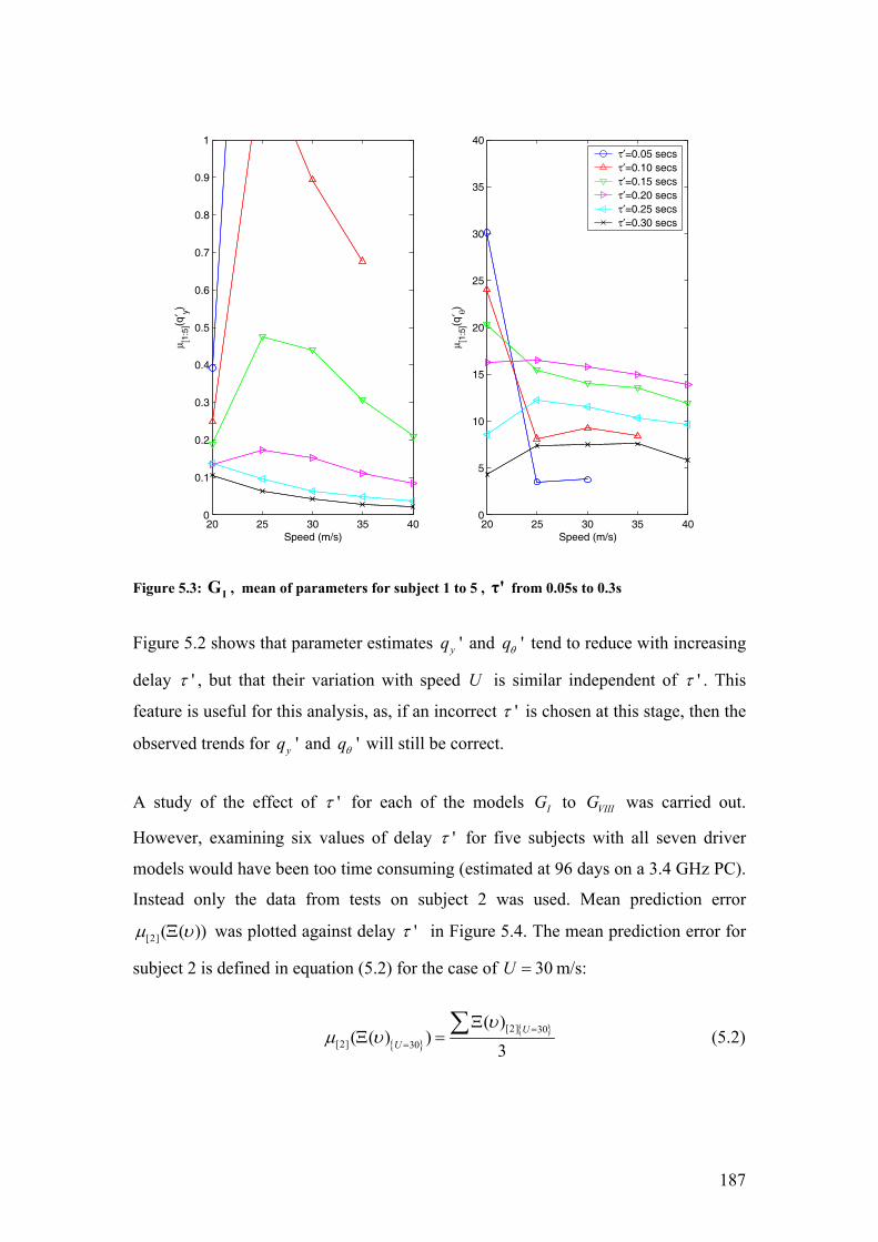
187
20 25 30 35 400
0.1
0.2
0.3
0.4
0.5
0.6
0.7
0.8
0.9
1
Speed (m/s)
µ [1:5
](q′ y)
20 25 30 35 400
5
10
15
20
25
30
35
40
Speed (m/s)
µ [1:5
](q′ θ)
τ′=0.05 secsτ′=0.10 secsτ′=0.15 secsτ′=0.20 secsτ′=0.25 secsτ′=0.30 secs
Figure 5.3: IG , mean of parameters for subject 1 to 5 , τ' from 0.05s to 0.3s
Figure 5.2 shows that parameter estimates 'yq and 'qθ tend to reduce with increasing
delay 'τ , but that their variation with speed U is similar independent of 'τ . This
feature is useful for this analysis, as, if an incorrect 'τ is chosen at this stage, then the
observed trends for 'yq and 'qθ will still be correct.
A study of the effect of 'τ for each of the models IG to VIIIG was carried out.
However, examining six values of delay 'τ for five subjects with all seven driver
models would have been too time consuming (estimated at 96 days on a 3.4 GHz PC).
Instead only the data from tests on subject 2 was used. Mean prediction error
[2] ( ( ))µ υΞ was plotted against delay 'τ in Figure 5.4. The mean prediction error for
subject 2 is defined in equation (5.2) for the case of 30U = m/s:
{ }{ }[2] 30
[2] 30
( )( ( ) )
3U
U
υµ υ =
=
ΞΞ =
∑ (5.2)

188
Identification at delay ' 0.05τ = s was not calculated for VIIG in order to speed up
identification for this model.
Figure 5.4: [2]µ (Ξ(υ)) for IG to VII G , subject 2 , 'τ from 0.05s to 0.3s
Model VIIIG is not included in Figure 5.4 because it is based on the same model as
VIIG , and both have almost identical prediction error [2] ( ( ))µ υΞ . Mean prediction
error for all subjects [1:5] ( ( ))µ υΞ for IG shown in Figure 5.2, and mean prediction
error for subject 2 [2] ( ( ))µ υΞ shown in Figure 5.4 are very similar. This gives
confidence that subject 2 is a good representation of the ensemble of subjects. This is
examined more thoroughly in section 5.2.2.
Models IG , IVG and VIIG have similar profiles of prediction error [2] ( ( ))µ υΞ vs.
delay 'τ . For all three of these models, delay ' 0.2τ = s gives minimum prediction
0.1 0.2 0.30
5
10
15
20
25
GI
µ [2](Ξ
(υ))
(/°)
0.1 0.2 0.30
5
10
15
20
25
GII
0.1 0.2 0.30
5
10
15
20
25
GIII
0.1 0.2 0.30
5
10
15
20
25
GIV
τ′ (/s)
µ [2](Ξ
(υ))
(/°)
0.1 0.2 0.30
5
10
15
20
25
GV
τ′ (/s)
U=20m/sU=25m/sU=30m/sU=35m/sU=40m/s
0.1 0.2 0.30
5
10
15
20
25
GVII
τ′ (/s)
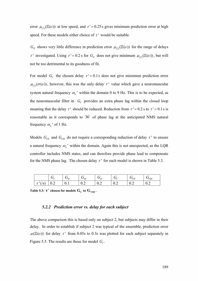
189
error [2] ( ( ))µ υΞ at low speed, and ' 0.25τ = s gives minimum prediction error at high
speed. For these models either choice of 'τ would be suitable.
IIG shows very little difference in prediction error [2] ( ( ))µ υΞ for the range of delays
'τ investigated. Using ' 0.2τ = s for IIG does not give minimum [2] ( ( ))µ υΞ , but will
not be too detrimental to its goodness of fit.
For model VG the chosen delay ' 0.1τ = s does not give minimum prediction error
[2] ( ( ))µ σ υ , however, this was the only delay 'τ value which gave a neuromuscular
system natural frequency 'nω within the domain 0 to 9 Hz. This is to be expected, as
the neuromuscular filter in VG provides an extra phase lag within the closed loop
meaning that the delay 'τ should be reduced. Reduction from ' 0.2τ = s to ' 0.1τ = s is
reasonable as it corresponds to 36 of phase lag at the anticipated NMS natural
frequency 'nω of 1 Hz.
Models VIIG and VIIIG do not require a corresponding reduction of delay 'τ to ensure
a natural frequency 'nω within the domain. Again this is not unexpected, as the LQR
controller includes NMS states, and can therefore provide phase lead to compensate
for the NMS phase lag. The chosen delay 'τ for each model is shown in Table 5.3.
IG IIG IIIG IVG VG VIIG VIIIG
'τ (/s) 0.2 0.1 0.2 0.2 0.2 0.2 0.2
Table 5.3: 'τ chosen for models IG to VIIIG .
5.2.2 Prediction error vs. delay for each subject
The above comparison this is based only on subject 2, but subjects may differ in their
delay. In order to establish if subject 2 was typical of the ensemble, prediction error
( ( ))µ υΞ for delay 'τ from 0.05s to 0.3s was plotted for each subject separately in
Figure 5.5. The results are those for model IG .

190
Figure 5.5: Ξ(υ) for IG , subjects 1 to 5 , τ' from 0.05s to 0.3s
Figure 5.5 shows that for subjects 2, 3, 4 and 5, minimum prediction error ( ( ))µ υΞ is
for a delay ' 0.2τ = s for the majority of speeds.
Subject 1 is the exception, with minimum prediction error ( ( ))µ υΞ for ' 0.3τ = s. This
suggests that Subject 1 had larger delay than average. This was borne out by
observations during testing that subject 1 had a noticeably slower response to errors
than other subjects. It is also notable that this subject was a novice with no training of
driving road cars, though some experience with driving in computer games.
It seems that Subject 2 was a good representative for the ensemble average to use in
the previous section (5.2.1) as his results are similar to the majority of subjects. The
dependence of goodness of fit ( ( ))µ υΞ on delay 'τ for the wider road width was not
0.1 0.2 0.30
5
10
15
20
25Subject 1
µ [1](Ξ
(υ))
/°
0.1 0.2 0.30
5
10
15
20
25Subject 2
0.1 0.2 0.30
5
10
15
20
25Subject 3
τ′ (/s)
0.1 0.2 0.30
5
10
15
20
25Subject 4
τ′ (/s)
µ [4](Ξ
(υ))
/°
0.1 0.2 0.30
5
10
15
20
25Subject 5
τ′ (/s)
U=20m/sU=25m/sU=30m/sU=35m/sU=40m/s

191
examined, but could be undertaken in future work. The difference in parameter
estimates ( ')yqµ and ( ')qθµ between subjects is examined in section 5.4.3.

192
5.3 Comparison of models
Having chosen an appropriate delay for all models, the fit of the models can now be
compared to establish which is best to represent the ensemble of drivers. The ‘best’
model can then be used to investigate differences between subjects, road widths and
speeds.
It is worth noting that a particular model may be better for a particular subject, e.g. a
novice subject may be better represented with a simpler model. However, the aim at
this stage is to try and find which model is best for the ensemble of subjects.
Goodness of fit is compared between the models in section 5.3.1. In section 5.3.2,
examples of steer angle time series are shown to illustrate the difference between the
models, and calibrate what a given level of prediction error ( )υΞ looks like. Noise
models are shown with each of these time series, and also how well the noise model is
fitting to the driver’s steer angle. The fitted model parameters 'yq and 'qθ are
compared between models IG to VIIIG in section 5.3.3. Finally, the resulting preview
controllers and state gains for IG to VIIIG are compared in section 5.3.4.
5.3.1 Goodness of fit
Having chosen a time delay 'τ for each model, the models can now be compared
directly. The mean prediction error across all five subjects [1:5] ( ( ))µ υΞ is used to
assess how well each model fits the ensemble of subjects. Prediction error [1:5] ( ( ))µ υΞ
vs. speed U for models IG to VIIIG on the 2.5m wide road is shown in Figure 5.6.

193
20 22 24 26 28 30 32 34 36 38 400
2
4
6
8
10
12
14
16
18
20
Speed U (m/s)
µ [1:5
](Ξ(υ
)) (
/°)
GI−2.5 m
GII−2.5 m
GIII−2.5 m
GIV−2.5 m
GV−2.5 m
GVII−2.5 m
GVIII
−2.5 m
Figure 5.6: [1:5]µ (Ξ(υ)) vs. speed for IG to VIIIG with τ' = 0.2 s ( τ' = 0.1s for IIG ), 2.5m width
Figure 5.6 shows that mean prediction error [1:5] ( ( ))µ υΞ increases with speed for all
models fitted. This implies either: worse model fit with increasing speed (increased
( )'G G u− in equation 4.11), or increasing driver noise with speed (increased He in
equation 4.11). It is difficult to distinguish the effects of model mismatch from the
effects of driver behaviour.
At low speed, all models have similar prediction error [1:5] ( ( ))µ υΞ , implying that all
are equally able to model driver behaviour at low speed. Additional model complexity
does not improve model fit for low speed driving.
At high speed IIG and IIIG give worse fit than IG . This implies that IG , which uses
both vehicle states ( ),ν ω reflects the behaviour of the ‘mean’ driver better than IIG
with no internal states, or IIIG with only a yaw rate state ( )ω . This implies that the
‘mean’ driver uses a vehicle controller with feedback of both ω and ν .

194
At high speed IG , IVG , VG , VIIG and VIIIG all give similar prediction error [1:5] ( ( ))µ υΞ ,
implying that the increased complexity of these models does not significantly improve
the fit over that of IG . The fact that all of the more complex models reach a similar
minimum prediction error [1:5] ( ( ))µ υΞ suggests either that ( )' 0G G− ≈ , or that the
drivers’ controller does not lie within the model set. It is, for example, possible that
the driver could be choosing sub-optimal controllers, leading to an increase in
( )'G G u− . Such sub-optimal controllers are not part of the LQR controller model set.
VIIG and VIIIG give slightly higher prediction error [1:5] ( ( ))µ υΞ than IG and IVG for
all speeds, implying that the inclusion of an NMS model has not helped to improve
the fit. Also VG gives a higher prediction error [1:5] ( ( ))µ υΞ than VIIG or VIIIG ,
suggesting that the internal NMS states of VIIG and VIIIG do improve the model fit.
IVG gives the lowest [1:5] ( ( ))µ υΞ of all models, for all speeds, but not by enough to
mark it as clearly the best model.
IG will be chosen to compare road widths and test subjects in the next section, as this
model gives nearly as low prediction error [1:5] ( ( ))µ υΞ as IVG but is simpler to
implement.
5.3.2 Time domain
Examples of time histories of δ for one driver, on one track are shown in this section.
These will not necessarily represent all data but are included to illustrate what is
meant by a given prediction error ( )υΞ . The examples also illustrate how the
controllers for IG to VIIIG differ, and allow comparison with the time histories of
chapter 3. The noise models are also plotted as solid lines in the lower subfigure, with
the PSD of the prediction error υ for that driver model shown as crosses of the
appropriate colour.
It must be remembered when examining time domain fits that steer angle is
unweighted in these plots, and that during optimisation it is the weighted steer angle
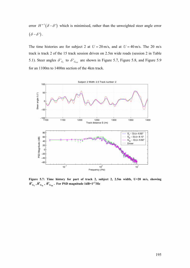
195
error ( )1' 'H δ δ− − which is minimised, rather than the unweighted steer angle error
( )'δ δ− .
The time histories are for subject 2 at 20U = m/s, and at 40U = m/s. The 20 m/s
track is track 2 of the 15 track session driven on 2.5m wide roads (session 2 in Table
5.1). Steer angles 'IGδ to '
VIIIGδ are shown in Figure 5.7, Figure 5.8, and Figure 5.9
for an 1100m to 1400m section of the 4km track.
1100 1150 1200 1250 1300 1350 1400−100
−50
0
50
100
Track distance S (/m)
Ste
er a
ngle
δ (
/°)
Subject: 2 Width: 2.5 Track number: 2
10−1
100
101
−60
−40
−20
0
20
40
60
80
PS
D M
agni
tude
(/d
B)
Frequency (/Hz)
GI − Ξ(υ)= 6.82°
GII − Ξ(υ)= 8.12°
GIII
− Ξ(υ)= 6.82°Driver
Figure 5.7: Time history for part of track 2, subject 2, 2.5m width, U=20 m/s, showing
IGδ' ,IIGδ' ,
IIIGδ' . For PSD magnitude 1dB=1°2/Hz

196
1100 1150 1200 1250 1300 1350 1400−100
−50
0
50
100
Track distance S (/m)
Ste
er a
ngle
δ (
/°)
Subject: 2 Width: 2.5 Track number: 2
10−1
100
101
−60
−40
−20
0
20
40
60
80
PS
D M
agni
tude
(/d
B)
Frequency (/Hz)
GI − Ξ(υ)= 6.82°
GIV
− Ξ(υ)= 6.4°G
V − Ξ(υ)= 7.67°
Driver
Figure 5.8: Time history for part of track 2, subject 2, 2.5m width, U=20 m/s, showing
IGδ' ,IVGδ' ,
VGδ' . For PSD magnitude 1dB=1°2/Hz
1100 1150 1200 1250 1300 1350 1400−100
−50
0
50
100
Track distance S (/m)
Ste
er a
ngle
δ (
/°)
Subject: 2 Width: 2.5 Track number: 2
10−1
100
101
−60
−40
−20
0
20
40
60
80
PS
D M
agni
tude
(/d
B)
Frequency (/Hz)
GI − Ξ(υ)= 6.82°
GVII
− Ξ(υ)= 6.96°G
VIII − Ξ(υ)= 7.01°
Driver
Figure 5.9: Time history for part of track 2, subject 2, 2.5m width, U=20 m/s, showing
IGδ' ,VIIGδ' ,
VIIIGδ' . For PSD magnitude 1dB=1°2/Hz

197
Figure 5.7, Figure 5.8, and Figure 5.9 show that there is little difference in steer angle
'δ between the identified models at low speed, which explains why all have similar
prediction error ( )υΞ .
It appears that oscillations at about 1 Hz in the steer angle δ of the real driver visible
in this sample are not being followed by the models, although the lower frequency
steer angle is correct. It was hoped that the NMS models could represent this
behaviour, but none of models VG , VIIG , or VIIIG show an improved fit. There is the
possibility that this behaviour may not be within the model set (e.g. be sub-optimal),
in which case none of the models could accurately represent it.
All of the noise models appear to fit well, and all of IG to VIIIG give similar noise
models at this speed. It appears that a lower order model could be used, but
identification does not suffer from ( , )yq qθ outliers, so the noise model order is not
too high.
The 40 m/s track is number 13 of 15, and '
IGδ to 'VIIIGδ are shown in Figure 5.10,
Figure 5.11 and Figure 5.12. Again an 1100m to 1400m section of the 4km track is
shown.
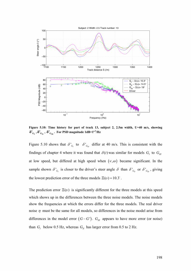
198
1100 1150 1200 1250 1300 1350 1400−100
−50
0
50
100
Track distance S (/m)
Ste
er a
ngle
δ (
/°)
Subject: 2 Width: 2.5 Track number: 13
10−1
100
101
−60
−40
−20
0
20
40
60
80
PS
D M
agni
tude
(/d
B)
Frequency (/Hz)
GI − Ξ(υ)= 10.3°
GII − Ξ(υ)= 14.5°
GIII
− Ξ(υ)= 19°Driver
Figure 5.10: Time history for part of track 13, subject 2, 2.5m width, U=40 m/s, showing
IGδ' ,IIGδ' ,
IIIGδ' . For PSD magnitude 1dB=1°2/Hz
Figure 5.10 shows that '
IGδ to 'IIIGδ differ at 40 m/s. This is consistent with the
findings of chapter 4 where it was found that ( )tδ was similar for models IG to IIIG
at low speed, but differed at high speed when ( ),ν ω became significant. In the
sample shown 'IGδ is closer to the driver’s steer angle δ than '
IIGδ or 'IIIGδ , giving
the lowest prediction error of the three models ( ) 10.3υΞ = .
The prediction error ( )υΞ is significantly different for the three models at this speed
which shows up in the differences between the three noise models. The noise models
show the frequencies at which the errors differ for the three models. The real driver
noise η must be the same for all models, so differences in the noise model arise from
differences in the model error ( )'G G− . IIIG appears to have more error (or noise)
than IG below 0.5 Hz, whereas IIG has larger error from 0.5 to 2 Hz.

199
1100 1150 1200 1250 1300 1350 1400−100
−50
0
50
100
Track distance S (/m)
Ste
er a
ngle
δ (
/°)
Subject: 2 Width: 2.5 Track number: 13
10−1
100
101
−60
−40
−20
0
20
40
60
80
PS
D M
agni
tude
(/d
B)
Frequency (/Hz)
GI − Ξ(υ)= 10.3°
GIV
− Ξ(υ)= 10.4°G
V − Ξ(υ)= 11.5°
Driver
Figure 5.11: Time history for part of track 13, subject 2, 2.5m width, U=40 m/s, showing
IGδ' ,IVGδ' ,
VGδ' . For PSD Magnitude 1dB=1°2/Hz
Examining models IG , IVG and VG in Figure 5.11, it can be seen that '
IVGδ is close
to that of 'IGδ , giving similar prediction error ( )υΞ for both. As seen in chapter 4, the
delay states only make slight differences to 'IVGδ , even at high speed.
The steer angle '
VGδ does not differ much from 'IGδ in the sample shown. Even at
this higher speed, the influence of the NMS is not visible in the steer angle. This may
be because the NMS is highly damped, meaning that it only has significant influence
above its natural frequency (approximately 2.5 Hz). The parameter values
{ }', ', ', 'y nq qθ ω ξ fitted to the models IG to VIIIG are described in section 5.3.3.
All three models have similar noise model shape at 40U = m/s, which is different to
that at 20 m/s. At 20 m/s there was a single cut-off frequency at 1 Hz, whereas at 40
m/s there are two cut-offs: one at 0.3Hz, and one at 2Hz. The noise model appears to
fit the features sufficiently well, so there is no need to increase the noise model order.

200
1100 1150 1200 1250 1300 1350 1400−100
−50
0
50
100
Track distance S (/m)
Ste
er a
ngle
δ (
/°)
Subject: 2 Width: 2.5 Track number: 13
10−1
100
101
−60
−40
−20
0
20
40
60
80
PS
D M
agni
tude
(/d
B)
Frequency (/Hz)
GI − Ξ(υ)= 10.3°
GVII
− Ξ(υ)= 11.5°G
VIII − Ξ(υ)= 11.5°
Driver
Figure 5.12: Time history for part of track 13, subject 2, 2.5m width, U=40 m/s, showing
IGδ' ,VIIGδ' ,
VIIIGδ' . For PSD magnitude 1dB=1°2/Hz
Examining models IG , VIIG and VIIIG in Figure 5.12, it can be seen that the steer
angles 'IGδ , '
VIIGδ , and 'VIIIGδ are very similar at high speed, with only small
differences in prediction error ( )υΞ between them. So, even at high speed, the NMS
has little influence on the steer angle of the models. Their noise models are again very
similar, with only slight differences apparent in the 0.3 to 0.4 Hz frequency range.
5.3.3 Model parameters
It is useful to compare the parameter estimates ( ', ')yq qθ and ( ', ')nω ξ for models IG
to VIIIG in order to show how their mean and variance differs between models, and
where these differences arise, particularly as for later analysis (section 5.4 onwards),
only model IG was used.
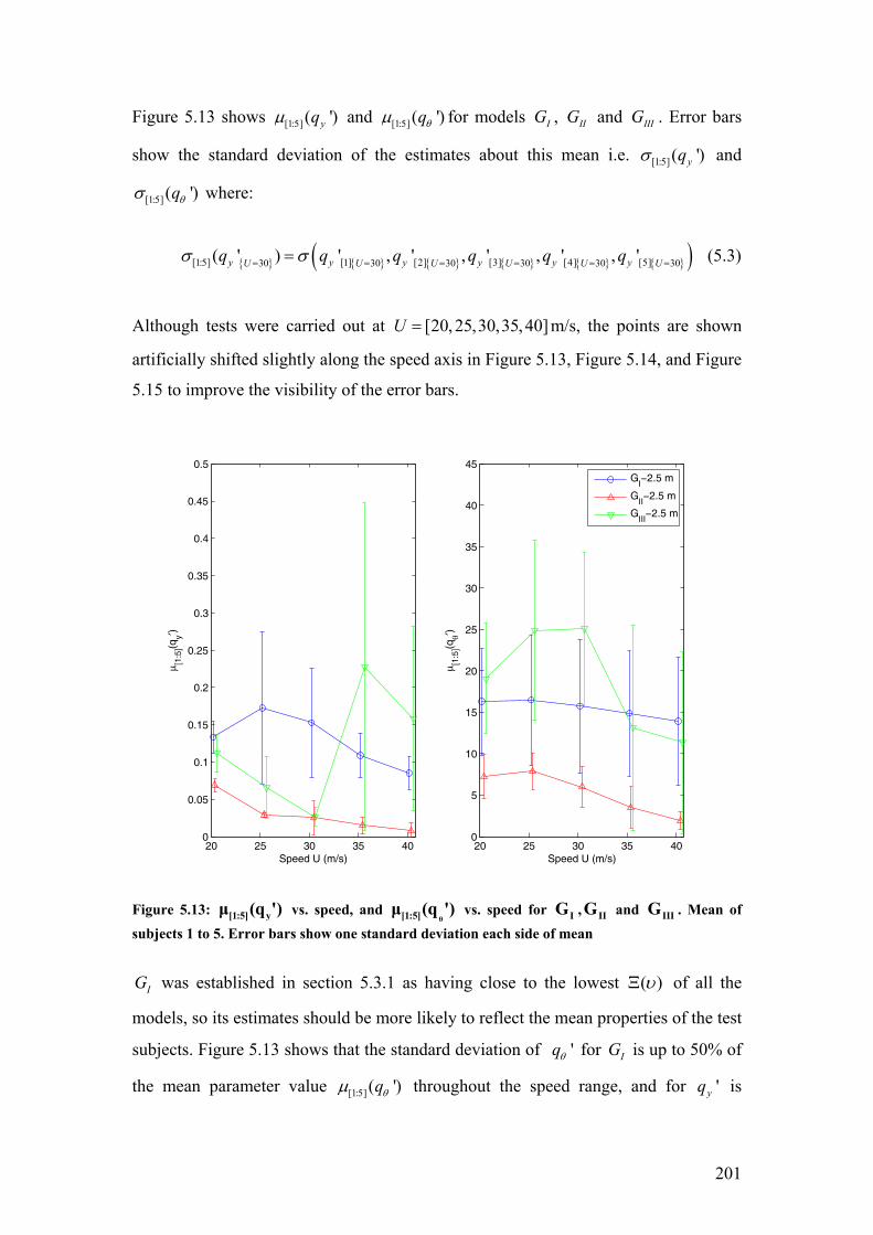
201
Figure 5.13 shows [1:5] ( ')yqµ and [1:5] ( ')qθµ for models IG , IIG and IIIG . Error bars
show the standard deviation of the estimates about this mean i.e. [1:5] ( ')yqσ and
[1:5] ( ')qθσ where:
{ } { } { } { } { } { }( )[1:5] [1] [2] [3] [4] [5]30 30 30 30 30 30( ' ) ' , ' , ' , ' , 'y y y y y yU U U U U Uq q q q q qσ σ= = = = = == (5.3)
Although tests were carried out at [20,25,30,35,40]U = m/s, the points are shown
artificially shifted slightly along the speed axis in Figure 5.13, Figure 5.14, and Figure
5.15 to improve the visibility of the error bars.
20 25 30 35 400
0.05
0.1
0.15
0.2
0.25
0.3
0.35
0.4
0.45
0.5
Speed U (m/s)
µ [1:5
](qy′)
20 25 30 35 400
5
10
15
20
25
30
35
40
45
Speed U (m/s)
µ [1:5
](qθ′)
G
I−2.5 m
GII−2.5 m
GIII−2.5 m
Figure 5.13: [1:5] yµ (q ') vs. speed, and
θ[1:5]µ (q ') vs. speed for IG , IIG and IIIG . Mean of subjects 1 to 5. Error bars show one standard deviation each side of mean
IG was established in section 5.3.1 as having close to the lowest ( )υΞ of all the
models, so its estimates should be more likely to reflect the mean properties of the test
subjects. Figure 5.13 shows that the standard deviation of 'qθ for IG is up to 50% of
the mean parameter value [1:5] ( ')qθµ throughout the speed range, and for 'yq is

202
between 10% and 50%. Parameter variance can arise from several sources: poor
model fit leading to biased estimates; poor consistency of control by the driver i.e.
changing their strategy between or during tests at a given speed; or from different
subjects using different controllers. This latter source is investigated in section 5.4.3
and is the primary cause of the large variance in 'qθ for IG .
Differences in 'yq and 'qθ between IG , IIG and IIIG are to be expected given that
each model has quite different steer angle for a given 'yq , 'qθ (as shown in chapter
4), and all are trying to fit to the same driver steer angle δ .
IIG had lower values of 'yq and 'qθ than the other two models throughout the speed
range, and showed a similar trend of reducing 'yq and 'qθ with speed. IIG had the
smallest parameter variance of the three models, implying that the parameter
estimates for each subject were repeatable, and also similar from subject to subject.
However, IIG also had the largest prediction error ( )υΞ (see Figure 5.6), so its fit is
least likely to reflect the properties of the driver during tests.
IIIG had a less clear pattern of 'yq and 'qθ with speed, and very large variance for the
35m/s result. High prediction error ( )υΞ suggested that this model was not suitable
for the ensemble of subjects, but it may be suitable for a novice driver.

203
20 25 30 35 400
0.05
0.1
0.15
0.2
0.25
0.3
0.35
0.4
0.45
0.5
Speed U (m/s)
µ [1:5
](qy′)
20 25 30 35 400
5
10
15
20
25
30
35
40
45
Speed U (m/s)
µ [1:5
](qθ′)
G
I−2.5 m
GIV−2.5 m
Figure 5.14: [1:5] yµ (q' ) vs. speed, and
θ[1:5]µ (q' ) vs. speed for IG and IVG . Mean of subjects 1 to 5. Error bars show one standard deviation each side of mean
Figure 5.14 shows that IVG had very similar variation of [1:5] ( ')yqµ and [1:5] ( ')qθµ
with speed to IG . However, for IVG both of the parameters [1:5] ( ')yqµ and [1:5] ( ')qθµ
are around 10% smaller than for IG . The standard deviations [1:5] ( ')yqσ and [1:5] ( ')qθσ
are also very similar for models IG and IVG . This is consistent with the two models
having very similar steer angle for a given ( , )yq qθ as shown in chapter 3.

204
20 25 30 35 400
0.2
0.4
0.6
0.8
1
Speed U (m/s)
µ [1:5
](qy′)
20 25 30 35 400
10
20
30
40
50
60
70
Speed U (m/s)
µ [1:5
](qθ′)
G
V−2.5 m
GVII−2.5 m
GVIII
−2.5 m
20 25 30 35 400
0.2
0.4
0.6
0.8
1
Speed U (m/s)
µ [1:5
] (ξ′
)
20 25 30 35 400
1
2
3
4
5
Speed U (m/s)
µ [1:5
](ωn′
) (
/Hz)
Figure 5.15: [1:5] yµ (q ') vs. speed,
θ[1:5]µ (q ') vs. speed, [1:5] nµ (ω ') vs. speed, and [1:5]µ (ξ') , for
VG , VIIG , and VIIIG . Mean of subjects 1 to 5. Error bars show one standard deviation each side of mean
Figure 5.15 shows that VG has much higher [1:5] ( ')yqµ than any other model, but
lower [1:5] ( ')qθµ which increases with speed, in contrast to other models. The presence
of the neuromuscular system filter without corresponding internal states clearly has a
marked effect on the resulting [1:5] ( ')yqµ and [1:5] ( ')qθµ selected. The yq estimates at
low speed are, however, very variable for VG .
The mean NMS natural frequency [1:5] ( ')nµ ω for model VG is significantly higher
than that for model VIIG . The fact that a larger phase delay NMS has been found for
model VIIG is consistent with the idea that the LQR controller in VIIG has some phase
lead due to its NMS state feedback and the time shifting of its preview gains. This
phase lead must be sufficient to overcome the phase delaying effect of a lower natural
frequency of NMS for model VIIG (around 1.5Hz as opposed to 3.5Hz for VG ). The
phase lead must also be sufficient to overcome the extra time delay of ' 0.2τ = s for

205
VIIG (whereas VG uses ' 0.1τ = s). Model VIIG has lower prediction error ( )υΞ than
VG , so the natural frequency estimate [1:5] ( ')nµ ω for VIIG is likely to be a more
accurate estimate than [1:5] ( ')nµ ω for VG . Though an intrinsic natural frequency of
3.7Hz was recorded by Pick [36] for tensed arms, active control of steer angle would
not be expected to be possible at this frequency due to delays in the reflex control
loop. It seems likely that the high NMS natural frequency of VG is an artefact of the
model’s poor fit, rather than a feature of the driver’s control.
For VIIG and VIIIG , the NMS parameters [1:5] ( ')nµ ω and [1:5] ( ')µ ξ are consistent for
the range of speeds, implying that NMS parameters are independent of speed for the
subjects tested.
The large variance of [1:5] ( ')yqµ for VIIG at 20U = m/s is consistent with the large
variance of identification seen for this model in the validation of chapter 4. Model
VIIG does not give the same [1:5] ( ')qθµ values as VIIIG despite being based on the same
model, because the NMS natural frequency nω for model VIIG does not exactly match
the 1 Hz that was assumed for model VIIIG . Similarly the NMS damping of model
VIIG of 0.45ξ = does not exactly match the values found for model VIIIG .
Overall, IG has similar [1:5] ( ')yqµ vs. speed, and [1:5] ( ')qθµ vs. speed to the other
models with low prediction error ( )υΞ ( IVG , VIIG and VIIIG ). The analysis of the
speed, subject and width dependence of these parameters [1:5] ( ')yqµ and [1:5] ( ')qθµ
will therefore be undertaken using model IG throughout section 5.4.
5.3.4 Preview controllers
The [1:5] ( ')yqµ and [1:5] ( ')qθµ values identified for IG to VIIIG differ from those
values investigated in chapter 3. It will therefore be useful to investigate the preview
controllers that arise from the parameter values identified in the previous section.
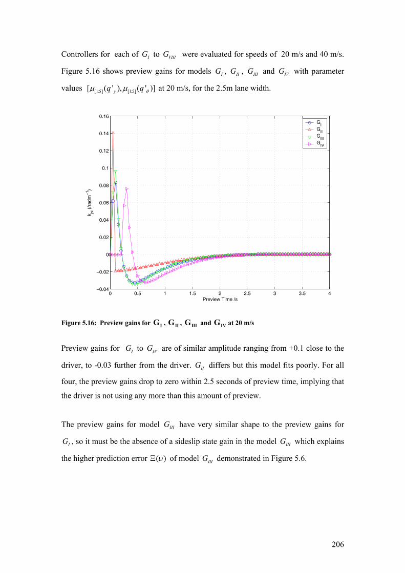
206
Controllers for each of IG to VIIIG were evaluated for speeds of 20 m/s and 40 m/s.
Figure 5.16 shows preview gains for models IG , IIG , IIIG and IVG with parameter
values [1:5] [1:5][ ( ' ), ( ' )]yq q θµ µ at 20 m/s, for the 2.5m lane width.
0 0.5 1 1.5 2 2.5 3 3.5 4−0.04
−0.02
0
0.02
0.04
0.06
0.08
0.1
0.12
0.14
0.16
Preview Time /s
k pi (
/rad
m−
1 )
GI
GII
GIII
GIV
Figure 5.16: Preview gains for IG , IIG , IIIG and IVG at 20 m/s
Preview gains for IG to IVG are of similar amplitude ranging from +0.1 close to the
driver, to -0.03 further from the driver. IIG differs but this model fits poorly. For all
four, the preview gains drop to zero within 2.5 seconds of preview time, implying that
the driver is not using any more than this amount of preview.
The preview gains for model IIIG have very similar shape to the preview gains for
IG , so it must be the absence of a sideslip state gain in the model IIIG which explains
the higher prediction error ( )υΞ of model IIIG demonstrated in Figure 5.6.

207
The different parameters [1:5] ( ' )yqµ and [1:5] ( ' )q θµ identified for each model have
resulted in quite similar preview gains. This is in contrast to the controllers shown in
chapter 4, where constant ( , )yq qθ were used, and led to quite different controllers.
0 0.5 1 1.5 2 2.5 3 3.5 4−0.06
−0.04
−0.02
0
0.02
0.04
0.06
0.08
0.1
Preview Time /s
k pi (
/rad
m− 1)
GI
GV
GVII
GVIII
Figure 5.17: Preview gains for IG , VG , VIIG and VIIIG at 20 m/s
Figure 5.17 shows preview gains for models IG , VG , VIIG and VIIIG with parameter
values [1:5] [1:5] [1:5] [1:5][ ( ' ), ( ' ), ( ' ), ( ')]y nq q θµ µ µ ω µ ξ at 20 m/s for the 2.5m lane width.
Again preview time is shorter than 2.5s so the preview of 4s used to derive the LQR
controllers was sufficient.
VG has the same LQR controller as IG , but different parameters [1:5] ( ' )yqµ and
[1:5] ( ' )q θµ have caused the preview gains to differ. This is likely to be in order to
compensate for presence of a NMS filter.
The controllers of VIIG and VIIIG give a similar time shift in their preview gains pik to
that of the delay state model IVG . All three of these controllers ( IVG , VIIG and VIIIG )
shift the peaks of the preview gains approximately 0.1 seconds further ahead of the

208
vehicle than those of IG . The similarity between the preview gains of IVG , VIIG and
VIIIG may indicate that the preview gains used by the driver are similar to these
controllers. Shifting of the preview gains enables the prediction error [1:5] ( ( ))µ υΞ of
these models ( IVG , VIIG and VIIIG ) to similar to that of model IG despite the extra
sources of lag present for these models (the delay dN for IVG and the NMS for VIIG
and VIIIG ).
VIIG and VIIIG have similar preview gains, but the differences in [1:5] ( ' )q θµ ,
[1:5] ( ' )nµ ω , and [1:5] ( ')µ ξ between the two models cause the gains to differ slightly.
VIIG has a ‘wavelength’ for its preview oscillations around 25% shorter than VIIIG .
This is consistent with the natural frequency of VIIIG being 30% lower
( { } 1 Hzn VIIIGω = , whereas { } 1.3 Hzn VIIGω = ). VIIIG therefore implies earlier steering
inputs by the driver than VIIG .
I III IV V VII VIII0
0.2
0.4
0.6
0.8
1
G
k ω /(
rad/
(rad
s−1
))
I IV V VII VIII0
0.02
0.04
0.06
0.08
0.1
0.12
G
k ν /(
rad/
(m s−1
))
VII VIII0
0.2
0.4
0.6
0.8
1
G
Sta
te g
ain
kδ /(rad/rad)
kdδ/dt
/(rad/(rad s−1))
0
0.05
0.1
0.15
0.2
kδ 4
kδ 3
kδ 2
kδ 1
Delay state
k δN
d−i /r
ad/r
ad
Figure 5.18: State gains for models IG to VIIIG at 20 m/s with
y θ n [1:5] y [1:5] θ [1:5] n [1:5][q ,q ,ω ,ξ] = [µ (q' ),µ (q' ),µ (ω' ),µ (ξ')]

209
Figure 5.18 shows state gains for models IG to VIIIG with parameter values
[1:5] [1:5] [1:5] [1:5][ ( ' ), ( ' ), ( ' ), ( ')]y nq q θµ µ µ ω µ ξ at 20 m/s for the 2.5m lane width. kω is
similar for all models which use this state gain. All models are within 20% of the
mean ( )kωµ . kυ differs by around 20% of the mean ( )kνµ between models except
for { }Vk Gυ which is notably higher. The high { }Vk Gυ comes about due to the high yq
value for this model at 20 m/s (see Figure 5.15).
kδ and d dtk δ for VIIG and VIIIG do differ significantly due to the differences in
[1:5] ( ' )q θµ , [1:5] ( ' )nµ ω and [1:5] ( ')µ ξ between the two models at 20 m/s.
The similarity of state and preview gains between models lends weight to the idea that
these gains are similar to the driver’s controller gains. However, the model set is
restricted to optimal LQR controllers, so this may be a facet of that restriction.
Figure 5.19 shows preview gains for models IG , IIG , IIIG and IVG with parameter
values [1:5] [1:5][ ( ' ), ( ' )]yq q θµ µ at 40 m/s for the 2.5m lane width.
0 0.5 1 1.5 2 2.5 3 3.5 4−0.04
−0.03
−0.02
−0.01
0
0.01
0.02
0.03
0.04
Preview Time /s
k pi (
/rad
m−
1 )
G
I
GII
GIII
GIV
Figure 5.19: Preview gains for IG , IIG , IIIG and IVG at 40 m/s

210
The preview gains pik for all controllers have changed from those at 20 m/s.
However, the preview gains for all controllers have reached zero a similar time ahead
of the vehicle to the controllers at 20m/s. This preview time of around 2 seconds
implies a doubling of the preview distance from that at 20 m/s.
IIIG has changed shape to be less similar to that of IG . It is at this speed that the
prediction error ( )υΞ is largest for model IIIG , so this controller is unlikely to closely
reflect the drivers’ controller.
0 0.5 1 1.5 2 2.5 3 3.5 4−0.04
−0.03
−0.02
−0.01
0
0.01
0.02
0.03
0.04
0.05
Preview Time /s
k pi (
/rad
m−
1 )
G
I
GV
GVII
GVIII
Figure 5.20: Preview gains for IG , VG , VIIG and VIIIG at 40 m/s
The preview gains for model VG are very similar to that of IG because the two LQR
models are the same, and have very similar [1:5] [1:5][ ( ' ), ( ' )]yq q θµ µ at this speed (see
Figure 5.15). Again the difference in preview gain ‘wavelength’ between VIIG and
VIIIG corresponds to the difference in 'nω between the two models.
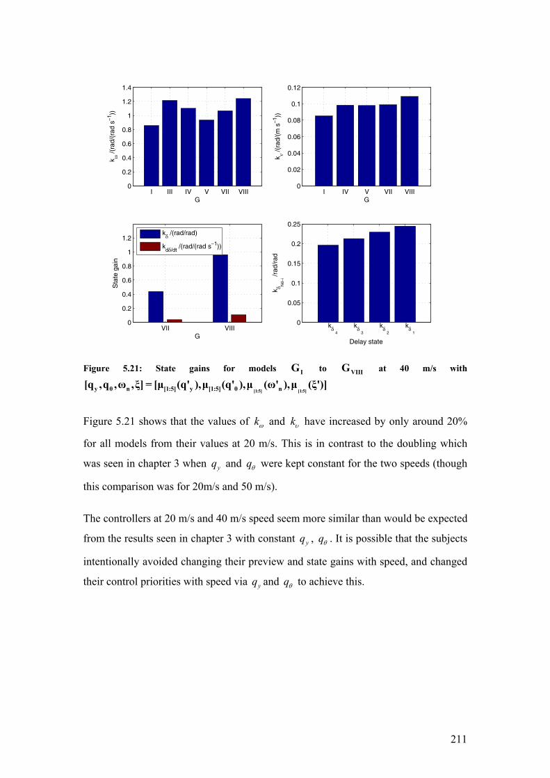
211
I III IV V VII VIII0
0.2
0.4
0.6
0.8
1
1.2
1.4
G
k ω /(
rad/
(rad
s−1
))
I IV V VII VIII0
0.02
0.04
0.06
0.08
0.1
0.12
G
k ν /(
rad/
(m s−1
))
VII VIII0
0.2
0.4
0.6
0.8
1
1.2
G
Sta
te g
ain
kδ /(rad/rad)
kdδ/dt
/(rad/(rad s−1))
0
0.05
0.1
0.15
0.2
0.25
kδ 4
kδ 3
kδ 2
kδ 1
Delay state
k δN
d−i /r
ad/r
ad
Figure 5.21: State gains for models IG to VIIIG at 40 m/s with
[1:5] [1:5]y θ n [1:5] y [1:5] θ n[q ,q ,ω ,ξ] = [µ (q' ),µ (q' ),µ (ω' ),µ (ξ')]
Figure 5.21 shows that the values of kω and kυ have increased by only around 20%
for all models from their values at 20 m/s. This is in contrast to the doubling which
was seen in chapter 3 when yq and qθ were kept constant for the two speeds (though
this comparison was for 20m/s and 50 m/s).
The controllers at 20 m/s and 40 m/s speed seem more similar than would be expected
from the results seen in chapter 3 with constant yq , qθ . It is possible that the subjects
intentionally avoided changing their preview and state gains with speed, and changed
their control priorities with speed via yq and qθ to achieve this.

212
5.4 Parameter variation with speed, width and subject
Having established that the models are fitting to the data, model parameters can now
be examined to see how they vary with the independent variables of the experiment,
namely test subject, vehicle speed, and lane width. IG was used as the driver model
for this analysis due to its combination of goodness of fit, and simplicity requiring
only parameters yq and qθ .
As previously, to analyse trends caused by one variable, parameters are averaged
across the other variables. The effect of speed and width will be dealt with in two
parts: their effect on lateral error and heading error in section 5.4.1; then their effect
on the parameters ( ', ')yq qθ in section 5.4.2. The variation of path error and ( ', ')yq qθ
as a function of speed should then enable the development of a new speed choice
model, which is discussed in section 5.5.
The experiments were designed in order to gather data for the variation of path error
with speed for a range of road widths, while at the same time measuring the
accompanying changes in driver effort or control strategy shown by yq and qθ .
Modifications were made to the hypothesis proposed in chapter 2 to account for the
inclusion of the controller weights yq and qθ .
It was hypothesised that for a given width 1W at low speed path error would stay
constant with increasing speed due to increased driver effort. This should show up in
increased yq and qθ , as shown by the blue lines in Figure 5.22. As speed continued to
increase the driver would run out of control effort, and path error would increase. This
is shown in Figure 5.22 where control effort (measured using controller weight q )
reaches a maximum maxq at speed 1U , above which the lateral error increases to
exceed the lane width. Figure 5.22 shows lateral error, but a similar trend was
anticipated for the heading error. It is this path error increase that would cause the
driver to have to limit their speed to 1U to stay within the road width.

213
For wider road this pattern was expected to be repeated, but with larger path error at
low speed due to the wider road. This would enable lower controller weights q to be
used by the driver to ease the control effort. This is shown as a red line in Figure
5.22. Again for low speeds control effort q would increase with speed to allow path
error to stay constant. As control effort was saturated at maxq at speed 2U , path error
would increase. The driver would therefore choose a higher speed 2U on the wider
road.
Figure 5.22: Hypothesised variation of path error and controller weights (q) with speed for lane widths 1W (blue) and 2W (red)
5.4.1 Path and heading error vs. width and speed
Figure 5.23 shows the steering controller parameters [1:5] ( )yqµ and [1:5] ( )qθµ and the
prediction error [1:5] ( ( ))µ υΞ in the upper three subplots. Figure 5.23 also shows the
mean 95th percentile lateral error [1:5] 95 0( ( ))pyµ ρ , mean 95th percentile heading error
[1:5] 95( ( ))µ ρ θ and mean 95th percentile driver steer angle [1:5] 95( ( ))µ ρ δ in the lower
three subplots. The figures are arranged to show the variables 0py , θ and δ involved
in the steering controller cost function (chapter 3 equation (3.9)), as well as the
resulting parameters yq and qθ . All parameters are shown for 2.5m, and 3.5m lane
width. The data from all subjects is averaged as before. As mentioned in section 5.1.2,
different speed ranges were used for each width in order to be easy to keep within the
road width at low speed, and very hard to keep within road width at the highest speed.
2W
1W
Speed U 1U 2U
yq or qθ
maxq
Speed U
Lateral error
1U 2U

214
Figure 5.23: Parameters vs. speed for widths 2.5 and 3.5m. IG fitted to all subjects
For the 2.5m wide road, lateral error ( [1:5] 95 0( ( ))pyµ ρ ) in the lower left plot and
heading error ( [1:5] 95( ( ))µ ρ θ ) in the lower centre plot were constant for low speeds (20
and 25 m/s). Above 25 m/s they increased, as expected.
For 3.5m lane width this sudden increase of lateral error and heading error with speed
is not visible. Also, the lateral error did not increase for the wider road as was
expected, and not by the amount that the available road width ( ) 2vW W− increased
(3 times). It is possible that the speed was not low enough, and that the curve would
flatten out for lower speeds giving constant lateral error for low speeds. However, this
minimum lateral error would still be much lower relative to the available road width
than was the case for the 2.5m road (see the dashed lines in the lower left subfigure
showing width of road available).
20 30 40 500
0.05
0.1
0.15
0.2
0.25
Speed U (m/s)
µ [1:5
](qy′)
20 30 40 500
5
10
15
20
25
30
Speed U (m/s)µ [1
:5](q
θ′)20 30 40 50
0
5
10
15
Speed U (m/s)
µ [1:5
](Ξ(υ
)) (
/°)
20 30 40 500
0.5
1
1.5
2
2.5
Speed U (m/s)
µ [1:5
](ρ95
(yp0
)) (
/m)
20 30 40 500
0.05
0.1
Speed U (m/s)
µ [1:5
](ρ95
(θ))
(/r
ad)
20 30 40 500
10
20
30
40
50
60
70
Speed U (m/s)
µ [1:5
](ρ95
(δ))
(/°)
GI−2.5 m
GI−3.5 m

215
In fact, contrary to expectation, there is slightly less lateral error on the wider road.
From the prediction error [1:5] ( ( ))µ υΞ it seems subjects produce more noise on the
narrower road for a given speed. This additional noise would then feed back to give
poorer path following (higher [1:5] 95 0( ( ))pyµ ρ and [1:5] 95( ( ))µ ρ θ ). Higher steer angle
[1:5] 95( ( ))µ ρ δ for a given speed on the narrower road is consistent with this.
This same reasoning could help to explain the sudden increase in [1:5] ( ( ))µ υΞ for the
2.5m road above 30 m/s, which could be caused by the increase in driver noise as
their muscle activity increases. It is known from work by Pick [36] that muscle
activation noise increases with muscle activity.
5.4.2 Parameters vs. width and speed
The changes of yq , qθ with speed have been mentioned throughout this chapter, but
not in the context of speed choice.
Figure 5.23 shows that for 2.5m width, yq increases with speed initially. This is
consistent with the idea that the driver initially keeps path error constant by increasing
control effort (increasing yq ). This increase in control effort shows up in the
increased steer angle [1:5] 95( ( ))µ ρ δ , with no increase in lateral error [1:5] 95 0( ( ))pyµ ρ .
Above 30 m/s yq decreases for both 2.5m and 3.5m width roads. At these speeds,
though the driver’s steering angle [1:5] 95( ( ))µ ρ δ does increase, the driver is unable to
increase input enough to keep their path error constant. The driver does not have
sufficient bandwidth to increase the steer angle at the frequency required to keep the
path error constant. For this LQR controller IG , with no output bandwidth limit, this
is equivalent to prioritising steer angle minimisation ahead of path error minimisation.
When road width is changed, the most marked parameter difference is in qθ . For the
wider road, qθ is increased by an average of 41.3% (for 30 to 40 m/s), and yq is

216
increased by an average of 20.0%. This change in qθ could indicate a difference in
driver attitude toward heading errors if there is more room to the edge of road.
Additional insight into the variation of yq and qθ with speed in Figure 5.23 can
usefully be gained by calculating ratios of steer angle to lateral error, and steer angle
to heading error.
[1:5] 95
[1:5] 95 0
( ( )( ( ))y
pyµ ρ δµ ρ
Π = (5.4)
[1:5] 95
[1:5] 95
( ( ))( ( ))θ
µ ρ δµ ρ θ
Π = (5.5)
The ratios yΠ and θΠ for the data from Figure 5.23 are shown in Figure 5.24:
20 30 40 500
20
40
60
80
100
120
Speed U (m/s)
Πy
20 30 40 500
200
400
600
800
1000
1200
Speed U (m/s)
Πθ
G
I−2.5 m
GI−3.5 m
Figure 5.24: yΠ vs. speed, and θΠ vs. speed for 2.5m, and 3.5m width, mean of results from all subjects
In many ways these results for yΠ and θΠ are consistent with the trends in
[1:5] ( ')yqµ , and [1:5] ( ')qθµ respectively.

217
For 2.5m width, yq increases with speed initially, corresponding to gradient of
[1:5] 95( ( ))µ ρ δ exceeding that of [1:5] 95 0( ( ))pyµ ρ . Above 30 m/s the trend for 2.5m and
3.5m looks similar, where yq decreases, corresponding to the gradient of
[1:5] 95 0( ( ))pyµ ρ exceeding that of [1:5] 95( ( ))µ ρ δ . In this case the driver does not
increase steering angle input enough to keep lateral error constant. The driver is
therefore prioritising steer angle minimisation ahead of lateral error minimisation.
The ratios yΠ and θΠ also make it easier to explain why qθ is nearly independent
of speed for both widths, because above 25 m/s, [1:5] 95( ( ))µ ρ θ and [1:5] 95( ( ))µ ρ δ have
similar gradient, corresponding to the nearly constant [1:5] ( ')qθµ .
What Figure 5.24 does not explain, though, is the difference in qθ for the two widths.
It might be expected that the change in [1:5] ( ')qθµ with width would give rise to a
change in the ratio θΠ whereas the ratio is the same for both widths. The decrease in
[1:5] 95( ( ))µ ρ δ from the 2.5m width to the 3.5m width is largely matched by the
decrease in heading error [1:5] 95( ( ))µ ρ θ . A similar observation applies to the (smaller)
change in [1:5] ( ')yqµ with width.
5.4.3 Parameters vs. subject
Comments in the previous sections refer to the ‘ensemble of subjects’ by using the
mean of parameters across all subjects. As was mentioned in the previous section, it is
possible that results from one atypical subject might have skewed the mean to be
unrepresentative of the ensemble.
In this section the subjects’ results are shown individually to examine differences
between subjects, and to establish whether the parameter mean is a fair representation
of the ensemble. It is also important to establish whether variance is caused by
individual subjects being variable, or by differences between subjects. Model IG is
used throughout this section with the results from the 2.5m road width.
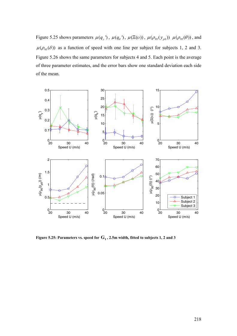
218
Figure 5.25 shows parameters ( ')yqµ , ( ')qθµ , ( ( ))µ υΞ , 95 0( ( ))pyµ ρ 95( ( ))µ ρ θ , and
95( ( ))µ ρ δ as a function of speed with one line per subject for subjects 1, 2 and 3.
Figure 5.26 shows the same parameters for subjects 4 and 5. Each point is the average
of three parameter estimates, and the error bars show one standard deviation each side
of the mean.
Figure 5.25: Parameters vs. speed for IG , 2.5m width, fitted to subjects 1, 2 and 3
20 30 400
0.1
0.2
0.3
0.4
0.5
Speed U (m/s)
µ(q y′)
20 30 400
5
10
15
20
25
30
Speed U (m/s)
µ(q θ′)
20 30 400
5
10
15
Speed U (m/s)µ(Ξ(υ)
) (
/°)
20 30 400
0.5
1
1.5
2
Speed U (m/s)
µ(ρ 95
(yp0
)) (
/m)
20 30 400
0.05
0.1
Speed U (m/s)
µ(ρ 95
(θ))
(/r
ad)
20 30 400
10
20
30
40
50
60
70
Speed U (m/s)
µ(ρ 95
(δ))
(/°)
Subject 1Subject 2Subject 3

219
Figure 5.26: Parameters vs. speed for IG fitted to subjects 4 and 5
The results show that individual subjects have low { }', 'yq qθ variance in most cases,
but that the means ( ')yqµ and ( ')qθµ differ between the subjects. An ensemble
average of the parameters from all subjects loses this information, and appears to have
large parameter variance.
Subject 3 achieves lower lateral error 95 0( ( ))pyµ ρ than other subjects by using larger
steer angle 95( ( ))µ ρ δ . This shows up as a higher ( ')yqµ than subject 2 for the 25 to
40 m/s range. This variation of ( ')yqµ is consistent with the ratio yΠ in section 5.4.2.
Subject 1 has higher lateral error 95 0( ( ))pyµ ρ than most of the other subjects. Subject
1 also has significantly higher heading error 95( ( ))µ ρ θ , but lower steer angle
95( ( ))µ ρ δ . This combination gives rise to much lower ( ')qθµ , consistent with ratio
20 30 400
0.1
0.2
0.3
0.4
0.5
Speed U (m/s)
µ(q y′)
20 30 400
5
10
15
20
25
30
Speed U (m/s)µ(
q θ′)
20 30 400
5
10
15
Speed U (m/s)
µ(Ξ(υ)
) (
/°)
20 30 400
0.5
1
1.5
2
Speed U (m/s)
µ(ρ 95
(yp0
)) (
/m)
20 30 400
0.05
0.1
Speed U (m/s)
µ(ρ 95
(θ))
(/r
ad)
20 30 400
10
20
30
40
50
60
70
Speed U (m/s)
µ(ρ 95
(δ))
(/°)
Subject 4Subject 5

220
θΠ , but not the expected reduction in yq which would be consistent with ratio yΠ .
It is likely that subject 1’s poor fit (large ( ( ))µ υΞ ) may explain the inconsistency
with ratio yΠ in this case.
Subject 1 has chosen a control strategy which weights reduced steer angle more than
reduced path error. Subject 1 is a non-driver, and had a visibly different attitude to the
driving task to the other subjects (less concerned about leaving the road). Given that
subject 1 was a non-driver it is possible that a simpler driver model could fit their
behaviour better. Figure 5.27 therefore shows prediction error ( ( ))µ υΞ vs. speed for
subjects 1 to 5 for IIG , the simplest driver model.
20 22 24 26 28 30 32 34 36 38 400
5
10
15
20
Speed U (m/s)
µ(Ξ(υ)
) (
/°)
Subject 1Subject 2Subject 3Subject 4Subject 5
Figure 5.27: µ(Ξ(υ)) vs. speed for subjects 1 to 5. for model IIG
It is clear from Figure 5.27 that subject 1 has the lowest prediction error ( ( ))µ υΞ , and
hence fits better to IIG than any other subject. This suggests that this novice subject is
better modelled without vehicle state gains. Subject 1 is not as well modelled by IIIG ,
suggesting that for this driver, the point mass model of the vehicle on which IIG is
based reflects their internal model of the vehicle more closely than the more

221
sophisticated IIIG . Given the discrepancy between subject 1 and the rest of the group,
it is tempting to exclude this subject from the ensemble. If subject 1 were excluded,
the mean of the parameter estimates of the remaining subjects could be used as a
representation of a ‘typical’ experienced driver using model IG . Subject 1 could then
represent a novice driver using model IIG . The controller weights and prediction error
for these two groups are shown for low and high speed in Table 5.4.
20 m/s 40 m/s Model
yq qθ ( )υΞ yq qθ ( )υΞ Subject 1 (novice) 1µ IIG 0.0546 8.48 7.63 0.0150 2.33 13.0 Subjects 2-5 (typical) 2:5µ IG 0.140 19.4 7.24 0.0809 16.8 10.5
Table 5.4: Mean parameter values for novice and typical subject groups, for 2.5m wide road.
Figure 5.25 and Figure 5.26 show that most subjects have similar gradients for
prediction error ( ( ))µ υΞ , lateral error 95 0( ( ))pyµ ρ and heading error 95( ( ))µ ρ θ with
speed, except subject 4. Subject 4 has similar values for these three parameters to the
other subjects at low speed, but much higher values at high speed. The high prediction
error ( ( ))µ υΞ for this subject at high speed contributes to the higher mean prediction
error for the ensemble [1:5] ( ( ))µ υΞ for the 2.5m width road seen in Figure 5.23.
In Figure 5.25 and Figure 5.26, the shape of ( ')yqµ and ( ')qθµ vs. speed is not
consistent between subjects, implying that each subject reacted differently to changes
in speed. Subjects 2, 3, 4 and 5 have similar parameter values for both ( ')yqµ and
( ')qθµ at low speed. However, whereas subjects 2 and 3 show a marked reduction in
( ')qθµ at high speed, subjects 4 and 5 show a slight increase in ( ')qθµ at high speed.
Both subjects 4 and 5 have larger steer angles 95( ( ))µ ρ δ at high speed than subjects 2
or 3, which is consistent with subjects 4 and 5 showing increased values of ( ')yqµ
and ( ')qθµ for these speeds (given that all four subjects have similar path error
95 0( ( ))pyµ ρ and 95( ( ))µ ρ θ ).

222
5.5 Implications for speed choice model
The use of these results to verify the speed choice hypothesis was not carried out
within the time frame of this work, and could be undertaken as future work as detailed
in chapter 6. However, there are some possibilities for a speed choice model which
can be identified at this stage from the results shown in section 5.4.1 and 5.4.2.
The lateral error vs. speed vs. width surface used for the speed choice hypothesis in
chapter 2 is available from this data. It should therefore be possible to test the original
hypothesis against this data. Both yq and qθ change with width, so the variation of
driver effort with width that was empirically represented in chapter 2 by the lateral
error percentile λ vs. width relationship could be replaced by a measure of driver
effort through yq and qθ .
Other speed choice hypotheses may also be possible given the new data. For example
the driver’s internal noise He (measurable using the prediction error ( ( ))µ υΞ )
changes with speed and width. It may be possible to use the variation in internal
noise as an alternative to path error as a cue to the driver’s speed choice. Such a
model might entail the driver using the internal noise as a measure of driving
‘comfort’, and limiting their speed choice to keep their internal noise below a
threshold level.
An alternative hypothesis might be based around the fact that the drivers’ preview
controller gains, and state gains were found to be fairly consistent with speed (section
5.3.4). It is possible that a driver could choose their speed in order to allow a constant
controller to be used. Speed could then be limited by the path width achievable with
this constant controller.
223
5.6 Conclusions
The identification procedure set out in chapter 4 was used to identify driver
parameters for data collected in simulator experiments on five subjects at a range of
speeds, and two lane widths. Ten iteration loops were found to be sufficient for
convergence to estimates 'yq and 'qθ . A [5/5] order noise model was found to be
flexible enough to fit well to the real driver data, and be of low enough order not to
cause 'yq and 'qθ outliers.
The weighted prediction error minimised during the identification ( )εΞ could not be
compared between different fits due to different noise models. So the unweighted
prediction error ( )υΞ was used to compare the goodness of fit of the models.
Time delay 'τ could not be identified reliably in the validation of chapter 4, so a
value of ' 0.2τ = s was used for most models based on values found from previous
research [36, 39]. ' 0.1τ = s was used for VG as it was the only value which gave an
NMS natural frequency 'nω within the domain (0 to 9 Hz). Changing 'τ was found to
affect only the magnitude of 'yq and 'qθ so any findings relating to the variation of
these parameters with speed would still be valid even if 'τ later turned out to be
incorrect.
Models IG to VIIIG were compared based on their prediction error ( )υΞ . IG , IVG ,
VIIG and VIIIG were found to give similar, low prediction error [1:5] ( ( ))µ υΞ for all
speeds, so were all suitable candidates for modelling the ensemble of subjects. IIG ,
IIIG and VG gave higher prediction error [1:5] ( ( ))µ υΞ than the other models especially
for higher speeds, meaning that they were not suitable to model the majority of
subjects. Model IG gave the best compromise between low prediction error ( )υΞ
and model simplicity so was used for later comparisons.
224
The parameter estimates 'yq and 'qθ were compared between the driver models.
Models IG , IVG , VIIG and VIIIG gave very similar yq and qθ because their steer
angles for a given yq and qθ were found to be similar in chapter 3. yq for VG
differed from all other models due to the presence of a neuromuscular filter which
does not feature in its LQR controller. Identified NMS parameters were constant for
the range of speeds. Model VIIG consistently gave 1.4nω ≈ Hz, and VIIIG consistently
gave 0.6ξ ≈ for all speeds. VG gave a different nω but gave higher prediction error
[1:5] ( ( ))µ υΞ .
The controller gains of the fitted driver models were compared at 20U = m/s, and
40U = m/s, as well as the time histories of the predicted steer angle. At 20U = m/s
the time histories of steer angle predicted by all models were similar, so their
prediction error ( )υΞ was also similar. Additional model complexity did not
therefore help to fit the driver data better at low speed. At 20 m/s all preview
controllers also had similar preview length and gain magnitudes. IVG , VIIG and VIIIG
all showed preview shifting by 0.1 seconds. This preview shifting negated the lagging
effect of the delay dN , and the NMS in these models.
At 40U = m/s, models IG , IVG , VG , VIIG and VIIIG all gave similar steer angles,
confirming the reason for their similar prediction error [1:5] ( ( ))µ υΞ . At 40U = m/s
models IIG and IIIG gave different steer angles to IG , and had much higher
prediction error [1:5] ( ( ))µ υΞ , implying their absence of vehicle state feedback made
them worse models of the behaviour of the majority of subjects. At 40 m/s the
preview gains for all models were only slightly changed from their counterparts at 20
m/s, giving a doubling of preview distance.
State gains were only 20% different for the two speeds 20U = m/s and 40U = m/s,
implying that the subjects may not change their vehicle state gains appreciably with
speed. Any differences in state gains between models did not appear to be correlated
to prediction error [1:5] ( ( ))µ υΞ , so the values of yq and qθ were not being fitted solely
to replicate a particular vehicle state gain used by the test subjects.
225
The variation of path error with lane width and vehicle speed were compared to the
expectation from a modified speed choice hypothesis. For 2.5m width, lateral error
[1:5] 95 0( ( ))pyµ ρ was constant at low speeds due to increasing driver steering activity
indicated by increased [1:5] 95( ( ))µ ρ δ . As speed increased, lateral error and heading
error increased as the driver’s internal noise He increased. The increase in He could
have been caused by increased steering activity. This observation agreed with the
expectation of the variation of path error with speed from the modified hypothesis.
For 3.5m width, contrary to expectation no sudden change in gradient of path error vs.
speed was found for increasing speed. For 3.5m width it was found that
[1:5] 95 0( ( ))pyµ ρ , [1:5] 95( ( ))µ ρ θ , [1:5] 95( ( ))µ ρ δ , and [1:5] ( ( ))µ υΞ all reduced slightly from
those of 2.5m. This could have been due to the reduced internal noise caused by the
lower steering activity.
The variation of 'yq and 'qθ with lane width and vehicle speed were also compared
to the expectation from the modified speed choice hypothesis. For the 2.5m wide road
at low speeds [1:5] ( ')yqµ increased with speed as expected indicating increased driver
effort. For higher speeds, [1:5] ( ')yqµ reduced with increasing speed as the increase in
lateral error exceeded the increase in steer angle, indicating a change in preference
toward steer angle minimisation rather than lateral error minimisation. Increased road
width gave a dramatic reduction in [1:5] ( ')qθµ , consistent with the idea that the driver
would reduce their weighting on heading error if the road edge was further away.
Ratios yΠ and θΠ were found to correlate with the variation of [1:5] ( ')yqµ and
[1:5] ( ')qθµ for a given width. They did not correlate well to the changes in [1:5] ( ')yqµ
and [1:5] ( ')qθµ between widths.
The path following errors, prediction errors, and steering controller weights were
compared between subjects. Most subjects’ results were found to fit well to the
ensemble means used earlier in the chapter. However, Subject 4 was found to have
higher internal noise than other subjects at high speed, leading to higher lateral error
95 0( ( ))pyµ ρ and heading error 95( ( ))µ ρ θ at high speed. Subject 1 was found to be

226
different to the other subjects in his attitude and path following ability. This was
thought to be due to the fact that subject 1 was a non-driver, and was found to be
better modelled by the simpler model IIG than by model IG .
Controller weights and prediction error were listed in Table 5.4 for two subject
groups: subjects 2 to 5 as a representation of typical experienced drivers using model
IG ; subject 1 as a representation of a novice driver using model IIG . Results were for
the 2.5m wide road only as the 3.5m wide road was not analysed separately for each
subject.
The possibility of using this data for the development of a revised speed choice model
was discussed. Some possible formulations were proposed, including using the
controller weights yq and qθ to replace the driver effort parameter identified in
chapter 2.
227
Chapter 6: Conclusions and future work A programme of work was carried out into the topic of driver speed choice. In this
chapter a summary of the work carried out and the main conclusions are given in
sections 6.1 and 6.2. The results highlighted some key areas for future work, which
are described in section 6.3.
6.1 Summary of work
6.1.1 Review of driver speed choice and steering models (Chapter 1)
In chapter one, speed choice was identified as an important factor in road accidents,
and also in driver learning. Improved understanding of speed choice could assist in
the design of roads and vehicles to aid more appropriate, and therefore safer, speed
choice. Research into the speed choice behaviour of drivers was therefore proposed.
The findings from the literature review and resulting research objectives can be
summarised as follows:
Path error based models of speed choice can predict the observed reduction in lateral
acceleration of drivers at high speed. However, the link between measured path error
and speed choice of drivers has not been examined. To examine this link, simulator
experiments to measure driver path error and speed choice as a function of road
geometry were proposed.
In order to model driver speed choice accurately, an understanding of the generation
of path error as a result of the driver’s steering control is required. To aid this
understanding, accurate models are required of the driver’s preview steering control
and how it varies with speed and road width. Models of preview steering control of
drivers are well developed, but bias free estimates of the preview model controller
weights used by drivers were not found in the literature. The development of
experiments and identification algorithms designed to minimise bias during the
identification of driver steering control models was therefore proposed.

228
Any differences between the steering control of experienced and inexperienced
drivers may be significant in the generation of different amounts of path error and
therefore different speed choice for experienced and inexperienced drivers. Driver
internal models with simplified vehicle dynamics have been proposed to represent the
less sophisticated preview control of a novice driver. However, these controllers have
not been demonstrated to give better fit to data collected from novice drivers than
controllers whose internal models have more sophisticated vehicle dynamics. It was
therefore proposed to develop models suitable for representing a novice driver, and fit
this model to measured driver data.
The effect of the driver’s neuromuscular system (NMS) on their steering control
bandwidth may be significant in the path error performance that can be achieved by
real drivers. It may therefore be important to include the effect of the driver’s NMS in
the formulation of driver steering models. Neuromuscular system models have been
studied and included in driver models, but had not been incorporated into the driver’s
internal model to represent a driver who modifies their control to take account of
knowledge of their own neuromuscular system. It was proposed that driver models be
developed to incorporate the effect of the NMS into the driver’s internal model. This
would allow assessment of the effect of including the driver’s knowledge of their own
bandwidth limitation on their preview controller. It might also provide a more
accurate driver model.
6.1.2 Driver speed choice modelling (Chapter 2)
In chapter two, data from a simulator test of speed choice were used to compare the
models of speed choice found in the literature review. From this analysis, none of the
models could provide all three requirements of good fit: a mechanistic model whose
assumptions were met by the fitted parameters and an ability to predict both the width
and radius dependence of speed choice.
A speed choice hypothesis was developed to incorporate the important features of the
previous models. This path error prediction hypothesis was assessed using measured
data from a simulator test.

229
During the simulator test, the subject’s lateral error was independent of bend
curvature, but his speed was not, indicating that his speed was changed in order to
keep lateral error constant. The subject’s lateral error changed with width, but not by
enough to keep the ratio of lateral error to available tolerance constant. This behaviour
was identified as either a risk strategy, or a change in steering control strategy (effort)
by the driver. A variable percentile of lateral error with width was added to the path
error based speed choice model to take account of this behaviour, but it was necessary
to assume constant driver effort.
A change of driver effort (or steering strategy) could not be ruled out in real driving
situations, so new experiments were proposed to measure changes in driver steering
strategy with speed and road width. These experiments were intended to determine if
changes in driver steering control strategy influenced driver speed choice. The
experiments proposed involved driving random roads at a range of fixed speeds, and a
range of road widths. The driver steering strategy was to be determined by fitting
preview steering control models to the measured steering control action of the driver.
6.1.3 Models of driver steering control (Chapter 3)
A requirement was identified in chapter two for a driver model which included a
steering strategy parameter, so models of the driver were developed based on Sharp’s
LQR controller structure. The models included cost function weights to allow the
driver’s strategy to be altered in favour of lateral error minimisation, heading error
minimisation, or steer angle minimisation.
In chapter one, the need was identified for models to represent the novice driver, and
to incorporate the effect of the NMS into the driver’s internal model. A driver model
with simplified vehicle dynamics was developed to represent novice drivers, and a
range of models including the driver’s neuromuscular system was also developed.
The following range of LQR controllers was developed:
230
• Model IG : Sharp’s controller using a 2DOF bicycle internal model.
• Model IIG : a point mass internal vehicle model to represent a novice driver.
• Model IIIG : a single degree of freedom internal model with no sideslip.
• Model IVG : as IG with added steer angle delay states.
• Model VG : internal model as IG , but with output steer angle filtered through
an NMS model
• Models VIG , VIIG and VIIIG : IG with added internal NMS states and output
steer angle filtered through an NMS model.
The preview and state gains of the controllers were compared for low and high speed.
Reasons for the differences in state gains and preview gains were explained based on
the differences between the models and changes in system dynamics with speed.
The driver models were simulated driving a vehicle along a random road path at low
and high speed, and with and without driver delay. The performance of the models
was compared and explained based on the differences found in their preview and state
gains. Models IVG , and VIG to VIIIG were found to give very similar steer angles to
IG due to good open loop inversion of the system being controlled. This was
achieved by preview shifting and additional state gains. Model VG had degraded
closed loop steering performance due to the presence of an NMS filter that was not
included in the LQR controller formulation.

231
6.1.4 Identification of driver steering models (Chapter 4):
It was necessary to ensure that models identified from driver data did not suffer from
identification bias, so chapter four developed the procedure necessary to ensure bias
free estimates from experimental data. An iterative procedure using the direct method
was designed for use in identifying driver model parameters.
Bias of identification was demonstrated when a white noise model was used to
identify data created using realistically coloured driver noise. A perfect noise model
eliminated bias when the driver noise was coloured.
Validation of the identification bias of the LQR controller cost function weights was
carried out using model IG for the following parameters: track PSD amplitude, road
spectral density roll-off gradient and track wavenumber cut-off. Suitable values were
determined for use in experiments. Vehicle speed was found not to affect
identification bias or variance.
A noise model of too low an order led to identification bias, but a noise model of too
high an order was prone to identification outliers. The order of the noise model had
therefore to be just sufficient to express the driver noise present.
Driver time delay was nearly perfectly identified when a perfect noise model was
used. However, with an identified (i.e. imperfect) noise model, time delay could not
be identified reliably for a realistic driver noise level.
Identification of each of the driver models IG to VIIIG was validated at a low and a
high speed with an identified noise model, but with correct time delay. Small bias was
found for model estimates 'IG to 'VG . 'VIG had very large variance of the identified
LQR controller weights, so was too unreliable for use in driver identification in
chapter five. 'VIIG and 'VIIIG were more successful than 'VIG at identifying NMS
parameters and cost function weights so were used for the identification of NMS
parameters in chapter five.

232
6.1.5 Driver model identification results (Chapter 5)
A requirement to determine the changes in control strategy of drivers with speed and
road width was identified in chapter two, so chapter five describes work aimed at
fulfilling this requirement.
Experiments were carried out on subjects using a fixed base simulator. Five subjects
drove roads at a set of fixed speeds, on two road widths. The identification procedure
set out in chapter four was used to identify driver parameters for data collected in the
simulator experiments. Sufficient iteration loops and noise model order were used to
reliably identify the data.
As demonstrated in chapter four, time delay could not be reliably identified, so a fixed
value was used. Changing the delay was found to affect the magnitude of the
controller cost function weights, but not their dependence on speed, so any findings
relating to the variation of these parameters with speed would still be valid even if the
chosen delay later turned out to be incorrect.
Models IG to VIIIG were compared based on their unweighted prediction error,
controller cost function weights, controller gains, and time histories of their predicted
steer angle. Models without vehicle state feedback gave poor fit to the behaviour of
the majority of subjects. Preview controllers and state gains for all models were found
to be similar for low and high speeds. Consistent NMS parameters were identified for
all speeds with model VIIG . Model IG was used for later comparisons as it gave very
close to the lowest prediction error and was simpler than model IVG .
The path following errors, prediction errors, and steering controller weights were
compared between subjects. Most subjects’ results were found to fit well to the
ensemble means used earlier in the chapter. However, the subject with no driving
experience differed from the other subjects and was found to be better modelled by
the driver model with a simplified internal vehicle model ( IIG ) than by model IG .

233
The variation of path error with lane width and vehicle speed were compared to the
expectation from a speed choice hypothesis modified to include steering controller
weights. For the narrower road width, the results agreed with the modified hypothesis.
For the wider road, contrary to expectation, no sudden change in gradient of path error
vs. speed was found for increasing speed. Path error and steering angle were found to
reduce as road width increased, possibly due to reduced internal noise caused by the
lower steering activity.
The variation of the cost function weights with lane width and vehicle speed was also
compared to the expectation from the modified speed choice hypothesis. The variation
of controller weights was not well predicted by the hypothesis, however, the variation
in lateral error weight with speed did indicate a change in preference toward steer
angle minimisation rather than lateral error minimisation as speed increased. Also, as
predicted, increasing road width gave a reduction in the heading error cost function
weight.
The possibility of using this data for the development of a revised speed choice model
was discussed. Some possible formulations were proposed, including using the LQR
controller cost function weights as the driver effort parameter identified in chapter
two.

234
6.2 Conclusions Driver speed choice modelling (Chapter 2):
• Driver steering control effort needs to be quantified for a successful path error
based speed choice model.
Models of driver steering control (Chapter 3):
• Models with added delay states and neuromuscular system states gave similar
steer angles to Sharp’s model when driven in closed loop with a vehicle. This
was due to good open loop inversion of the system dynamics by preview
shifting and their additional state gains.
Identification of driver steering models (Chapter 4):
• The elimination of identification bias was demonstrated using an iterative
algorithm based on Ljung’s direct method.
o Parameters were found for a random road excitation to give successful
identification of artificially created driver data.
o Time delay could not be identified with an identified noise model.
o Too low noise model order was found to give bias, and too high order
gave outliers.
• The algorithm was proven to give correct identification with each of the driver
models derived in chapter 3 at 20m/s and 50 m/s.
o All models except the 6 state NMS model could be identified with a
bias of the steering controller weightings of less than 6.2%, and
variance of less than 36.7%.
o The bias and variance of the lateral error weighting yq was around 1/3
of those of the heading error weighting qθ .
o For the 6 state NMS model, bias and variance were too high if both
NMS parameters were identified at the same time, so was not used for
identification.

235
o Identifying the NMS parameters with separate models gave improved
bias of less than 15.4% for the controller weights, but up to 31.5% for
the NMS damping. Variance was as high as 66.5% for the heading
error weight, and 136% for the NMS damping.
Driver model identification results (Chapter 5)
• The algorithm validated in chapter 4 was used to fit seven models to data from
five drivers on two road widths at a range of speeds. Unbiased controller
weightings and prediction error were derived, allowing comparison of subjects
and models as a function of road width and vehicle speed.
• The assumed driver delay was found to affect the values of the controller
weights, but not their trends with speed, so a delay of 0.2s was assumed.
• Differences between the fitted models were found when comparing their
prediction error and derived model parameters for data from the narrow road.
o Similar state and preview gains were seen for most models, suggesting
that these gains may be similar to those of the real drivers.
o All fitted models gave similar steer angles to Sharp’s model at low
speed, hence similar prediction error, but those with simplified internal
models gave poor fit at high speed.
o Including an NMS did not improve model fit, but inclusion of delay
states gave a slight improvement in the unweighted prediction error.
o Consistent NMS parameters were identified for a range of speeds with
a mean natural frequency of 1.35 Hz and damping coefficient of 0.59.
• Differences in behaviour between subjects were found on the narrow road
which could be interpreted as differences between novice and experienced
drivers.
o The point mass driver model was found to be the most suitable model
for the novice subject, whereas Sharp’s model was the most suitable
model for the experienced subjects.
• Changes in driver control strategy were found as a function of speed and road
width using the fitted results from Sharp’s model for the ensemble of subjects.
o Contrary to expectation, path error reduced for increased road width,
possibly due to reduced driver noise.

236
o Increased road width from 2.5m to 3.5m gave a 41.3% reduction in
heading error weight, but an unexpected 20.0% increase in lateral error
weight.
o A modified speed choice hypothesis correctly predicted the variation
of path error and steer angle with speed for the narrow road, but not for
the wider road.
o Similar state and preview gains were seen for all speeds suggesting
drivers may keep a constant controller for a range of speeds.

237
6.3 Recommendations for future work
The results and conclusions of this work highlighted some key areas for future work.
6.3.1 Analysis of full interactions
A detailed analysis of all of the data should be undertaken to determine the
interactions between parameters now that the important first order effects have been
shown.
The analysis of parameter changes with speed, width and subject was carried out
using only driver model IG . This same analysis should be carried out at least on
models VIIG and IVG . The former because it includes a neuromuscular system, and
the latter because it gave lower prediction error than IG , and may therefore be a better
model of the driver.
Also, the parameter variations with each subject were only compared for the narrower
road. A similar comparison should also be carried out for the wider road, to give
insight into the reasons for ensemble parameter changes on the wider road.
6.3.2 Derived model validation
The direct method fitting procedure was validated in chapter five, but the models
fitted in chapter five have not been validated. The next step is to simulate these
controllers in closed loop with a vehicle to check that they reflect the behaviour of a
real driver.
Also, a method should be found to identify, rather than presume a driver delay. The
dependence of driver delay on subject, width, and speed could then be determined,
and model fit may be improved.
238
6.3.3 Larger model set The model set is currently restricted to LQR preview models, but model predictive
control (MPC) might usefully represent the driver’s reaction to the constraints
provided by the road edges. Alternatively, the cost function used for the LQR model
could be modified to include other driver effort measures beyond simply steer angle.
Finally, a more sophisticated neuromuscular model could be developed, as the NMS
used in this work did not significantly improve the fit of the model.
6.3.4 Hypothesis for path error vs. speed
Use should be made of the free speed choice data gathered during the experiments
described in chapter five. The speed choice models proposed in chapter five
incorporating the measured preview model cost function weights could be validated
using these data.
6.3.5 Further testing
With the increasing availability of accurate vehicle positioning systems an assessment
of path error and speed choice of drivers in real vehicles could be undertaken to
further validate a path error based speed choice model. This would allow the influence
of realistic non-linear vehicle dynamics, and more realistic driver risk stimuli to be
assessed. As an intermediate step, tests on a moving base simulator, and the inclusion
of more realistic steering torque feedback would give useful insight.
6.3.6 Driver learning
The interconnection between speed choice and driver learning of the steering control
task was outlined in the introduction to this dissertation. If a validated model of driver
steering control (such as that described in this dissertation) could be linked to a path
error based speed choice model, a closed loop driver steering and speed choice model
could be constructed. This model could be used to explore the effect on speed choice

239
of the driver’s learning of their own steering competence by interpolation and
extrapolation of their path error vs. speed vs. curvature surface. This would be
particularly important for a non-linear vehicle model, where the more complex
dependence of vehicle dynamics on vehicle states might lead to the driver making
poor predictions of their path error, and hence poor speed choices. This would in turn
affect the driver’s learning of the non-linear vehicle dynamics.

240
Appendix A: Vehicle model parameters The parameters used for the vehicle model for the 180° curve tests in chapter 2 are
shown in Table A.6.1. The parameters used for the vehicle model for chapters 3, 4
and 5 are shown in Table A.6.2.
Variable Value Units
fC 152386 N/rad Front axle tyre stiffness
rC 152386 N/rad Rear axle tyre stiffness a 1.31 m Front axle to CG distance b 1.31 m Rear axle to CG distance L 2.62 m Wheelbase of vehicle M 1673 Kg Mass of vehicle I 2550 Kg m2 Yaw moment of inertia of vehicle
vW 2.0 m Vehicle width
swK 16 - Steer angle to wheel angle gain
Table A.6.1: Parameters used for vehicle model for 180º curve tests of (chapter 2)
Variable Value Units
fC 152386 N/rad Front axle tyre stiffness
rC 152386 N/rad Rear axle tyre stiffness a 1.2 m Front axle to CG distance b 1.4 m Rear axle to CG distance L 2.6 m Wheelbase of vehicle M 1673 Kg Mass of vehicle I 2811 Kg m2 Yaw moment of inertia of vehicle
swK 16 - Steer angle to wheel angle gain
vW 2.0 m Vehicle width
colK 0.08 N m/deg Spring return on column angle stiffness
colλ 0.004 Nms/deg Damping on column velocity
Table A.6.2: Parameters used for vehicle testing for random roads (chapters 3 to 5)

241
Appendix B: Simulator vehicle longitudinal dynamics model
Figure B.1: Free body diagram of longitudinal vehicle model
max 2. . .thrd rollengine drag roll
PF F F U AC F M UUφ
− − = − − = (B.1)
where:
engineF = Engine thrust rollF = Rolling resistance dragF = Aerodynamic drag force maxP = Max engine power (1000 kW)
thφ = Throttle proportion (from –1 to 1) U = Forward speed
1 dAC = Frontal Area (4 m2) x Aero drag coefficient M = Vehicle mass
engineF is a forward force from the engine, whose power output is proportional to
throttle proportion. dragF is a simplified aerodynamic drag force term, while rollF is a
frictional rolling resistance. A saturator ensures that longitudinal force cannot exceed
that necessary to produce an acceleration of 1g as a model of the traction limit of the
tyres. The values of these parameters are not chosen to reflect any specific car’s
performance (e.g. 1000 kW engine used is very large) though they are qualitatively
realistic, but are chosen to allow the driver to change speed easily with little
requirement to plan ahead their speed changes.
Car ( M )
engineFdragF
rollF
U

242
Appendix C: Lateral error calculation for 180º curves Lateral error estimation for 180º curves depends on which part of the curve is being
traversed, the straight, transition, or constant curvature part. For the straight error
equals the lateral offset position y. For the constant curvature part error is the
difference between the curve radius and the distance of the car from the centre point
of the arc. For the transition in Figure C.1, an iterative routine is used to find the point
on the path (P) whose perpendicular passes through the vehicle’s position (A). The
distance ( 0py ) between this point and the vehicle’s position is then evaluated.
Figure C.1: Lateral error calculation for transition section
A
x
y
0py
P R ψ−
a

243
Appendix D: Lateral error evaluation using intrinsic co-ordinates
An algorithm for ‘on the fly’ calculation of lateral error normal to the intended path of
the vehicle was derived from first principles. Input is an intrinsic road profile, with
sufficient resolution to approximate a continuous profile. The resolution necessary
will depend on the wavelength content of the profile, however, 0.1m resolution was
found to be adequate. The vehicle trajectory is determined from the vehicle states
( ),ν θ and the forward speed U.
Figure D.1: Geometric definitions for derivation of intrinsic lateral error estimation
From Figure D.1: t tS R ψ∂ = ∂ (D.1) ( )err t err tn R Y S Yψ ψ∂ = + ∂ = ∂ + ∂ (D.2) cos( )err t err tS n S Yψ ψ∂ = ∂ = ∂ + ∂ (D.3)
cos( )
tt err t
t
err
x Y SSS
ψ
ψ
∂∂ + ∂
∂∂ = (D.4)
tψ∂
S∂ R
errψ errY
errY∂
tS∂
Actual Vehicle Path ( ),S ψ
n∂
Road Path ( ),t tS ψ

244
So as 0S∂ ⇒ :
cos( )
1
t err
terr
t
dSddS YdS
ψψ=
+ (D.5)
Note that: 2 2dS U dtν= + (D.6) err tψ ψ ψ= − (D.7)
Uνψ θ= + (D.8)
So as a function of time equation (D.5) becomes (using equation(D.6)):
2 2cos( )
1
t t
terr
t
dS Uddt YdS
ψ ψ νψ
− +=
+ (D.9)
Similar equations can be derived for lateral displacement from the path (lateral error): sin( )err errY S ψ∂ = ∂ (D.10)
So as 0s∂ ⇒ , and incorporating equation (D.6) and (D.7):
2 2sin( )errt
dY Udt
ψ ψ ν= − + (D.11)
In implementing an algorithm for evaluation of tS and errY from equations (D.9) and
(D.11) the correct values of tψ and t
t
ddSψ must be determined at the present point in
the track. This is defined by the present value of tS , and requires lookup tables of
these variables to be used. Figure D.2 shows a flow diagram of the above algorithm
used in MATLAB Simulink during simulator tests.

245
Figure D.2: Flow diagram for intrinsic lateral error estimation using MATLAB Simulink
Lookup { }t tSψ
Lookup
{ }tt
t
d SdSψ
arctan
cos 1s
1s
sin
U
ν
2 2U ν+
2 2U ν+
errY θ
1
tS +
−
+
+
× ÷
+ +
÷
×errψ
×
×
×
×
×
×
246
Appendix E: White noise curvature case in random road profiles A value of 2γ = − is significant because it corresponds to a white noise track
curvature spectrum as shown in equations (E.1) to (E.4). Firstly, for white curvature
input, spectral density of curvature ( )td
dSψ χ
Φ
must be white:
( ) K td
dSψ χΦ = (E.1)
Curvature spectral density corresponds to angle spectral density according to:
2( ) ( )t td
dSψ ψχ χ χ−Φ = Φ (E.2)
Equations (E.1) and (E.2) lead to the following angle spectral density profile for a
white curvature spectrum:
2( ) Ktψ χ χΦ = (E.3)
Which implies the following parameters for a road profile:
2K
γκ= −=
(E.4)

247
References
[1] Sabey, B. How fast is fast enough? in Scottish Road Safety Campaign Seminar, Killing speed saving lives. 1993.
[2] Carsten, O.M.J., et al., Urban Accidents: Why do they happen? 1989, AA Foundation for Road Safety Research, Basingstoke.
[3] Maycock, G., Brocklebank, P.J., and Hall, Road layout design standards and driver behaviour. 1998, Transport Research Laboratory TRL, Crowthorne. Report no. 332.
[4] Quimby, A., et al., The factors that influence a drivers choice of speed a questionnaire study. 1999, Transport Research Laboratory TRL, Crowthorne. Report no. 325.
[5] Quimby, A., et al., Drivers speed choice an in-depth study. 1999, Transport Research Laboratory TRL, Crowthorne, Report no. 326.
[6] Taylor, M., Lynam, D., and Baruya, A., The effects of drivers speed on the frequency of road accidents. 2000, Transport Research Laboratory TRL, Crowthorne.
[7] Winkler, C.B., et al., Rollover of commercial vehicles. SAE, 2000. [8] Winkler, C.B., et al., Evaluation of Innovative Converter Dollies. 1993,
University of Michigan Transportation Research Institute, Ann Arbour, MI, USA.
[9] Kusters, J.J., Increasing Roll-Over Safety of Commercial Vehicles by Application of Electronic Systems, in Smart Vehicles, J.P. Pauwelussen and Pacejka, H.B., Editors. 1995. p. 326-377.
[10] Levison, W.H., Interactive Highway Safety Design Model: Issues Related to Driver Modeling. Transportation Research Record, 1998. 1631: p. 20-27.
[11] Russell, S. and Norvig, P., Artificial Intelligence. 3rd ed. 1995: Prentice-Hall, New Jersey.
[12] Ritchie, M.L., McCoy, W.K., and Welde, W.L., A Study of the Relation Between Forward Velocity and Lateral Acceleration in Curves During Normal Driving. Human Factors, 1968. 10(3): p. 255-258.
[13] Drury, C.G., Movements with Lateral Constraint. Ergonomics, 1971. 14(2): p. 293-305.
[14] Glennon, J.A. and Weaver, G.D., The Relationship of Vehicle Paths to Highway Curve Design. 1971, Texas Transportation Institute report. p. 134-135.
[15] Herrin, G.D. and Neuhardt, J.B., An Empirical Model for Automobile Driver Horizontal Curve Negotiation. Human Factors, 1974. 16(2): p. 129-133.
[16] McLean, J.R., Driver Behaviour on Curves - A Review. ARRB Proceedings, 1974. 7(5): p. 129-147.
[17] Taragin, A., Driver performance on horizontal curves. Proc. Highway Research Board., 1954. 33.
[18] Emmerson, J., Speed of cars and sharp horizontal curves. Traffic Engineering and Control, 1969: p. 135-137.
[19] Felipe, E. and Navin, F., Automobiles on Horizontal Curves, Experiments and Observations. Transportation Research Record, 1998. 1628: p. 50-56.

248
[20] Bottoms, D.J., The interaction of driving speed, steering difficulty and lateral tolerance with particular reference to agriculture. Ergonomics, 1983. 26(2): p. 123- 139.
[21] DeFazio, K., Wittman, D., and Drury, C.G., Effective Vehicle Width in Self-Paced Tracking. Applied Ergonomics, 1992. 23(6): p. 382-386.
[22] Cole, D.J., Influence of Vehicle Response on the Driver's Preview Control of Speed. EPSRC Research Proposal, 2002, CUED.
[23] Reymond, G., et al., Role of Lateral Acceleration in Curve Driving: Driver Model and Experiments on a Real Vehicle and a Driving Simulator. Human Factors, 2001. 43(3): p. 483-495.
[24] Van Winsum, W. and Godthelp, H., Speed Choice and Steering Behaviour in Curve Driving. Human Factors, 1996. 38(3): p. 434-441.
[25] Savkoor, A.R. and Ausejo, S., Analysis of driver's steering and speed control strategies in curve negotiation. Vehicle System Dynamics, 2000. v 33(n Suppl): p. p 94-109.
[26] Wade, A.R., Rosenthal, T.J., and Hogue, J.R., Modeling and simulation of driver/vehicle interaction. SAE Special Publications, 1996(n 1141): p. p 27.
[27] Sharp, R.S., Casanova, D., and Symonds, P., A mathematical model for driver steering control, with design, tuning and performance results. Vehicle System Dynamics, 2000. 33(5): p. 289-326.
[28] Prokop, G., Modeling Human Vehicle Driving by Model Predictive Online Optimisation. VSD, 2001. 35(1): p. 19-53.
[29] Denton, G.G., A Subjective Scale of Speed when Driving a Motor Vehicle. Ergonomics, 1966. 9(3): p. 203-210.
[30] Denton, G.G., The Influence of Adaptation on Subjective Velocity for an Observer in Simulated Rectilinear Motion. Ergonomics, 1976. 19(4): p. 409-430.
[31] Fineberg, M.L., The Effects of Previous learning on the Visual Perception of Velocity. Human Factors, 1977. 19(2): p. 157-162.
[32] Matthews, M.L. and Cousins, L.R., The Role of Vehicle Characteristics in Drivers' Perception of Automobile Velocity. Proceedings of the Human Factors Society, 1978. 22: p. 110-114.
[33] Salvatore, S., The Estimation of Vehicular Velocity as a Function of Visual Stimulation. Human Factors, 1968. 10(1): p. 27-32.
[34] Gawron, V.J. and Ranney, T.A., Curve Negotiation Performance in a Driving Simulator as a Function of Curve Geometry. Applied Ergonomics, 1990. 21(1): p. 22-38.
[35] Guo, K. and Guan, H., Modelling of Driver/Vehicle Directional Control System. VSD, 1993. 22: p. 141-184.
[36] Pick, A.J., Neuromuscular Dynamics and the Steering Task, PhD Thesis, Engineering Department, Cambridge University.
[37] Rutherford, S., Driver Speed Choice and Vehicle Handling, MEng Thesis, Engineering Department, Cambridge University.
[38] McRuer, D.T. and Krendel, E.S., The Human Operator as a Servo System Element Part II. Journal of the Franklin Institute, 1959. 267: p. 511-536.
[39] McRuer, D.T. and Krendel, E.S., The Man-Machine System Concept. Proceedings of the IRE, 1962: p. 1117-1123.
[40] Weir, D.H. and McRuer, D.T., Dynamics of Driver Vehicle Steering Control. Automatica, 1970. 6: p. 87-98.

249
[41] MacAdam, C.C., Application of an Optimal Preview Control for Simulation of Closed-Loop Automobile Driving. IEEE Trans, 1981. SMC-11(6): p. 393-399.
[42] Peng, H., Evaluation of driver assistance systems - a human centred approach. Proceedings AVEC, 2002.
[43] Sharp, R.S. and Valtetsiotis, V., Optimal Preview Car Steering Control. VSD, 2001. Supp 35: p. 101-117.
[44] Maciejowski, J.M., Predictive Control with Constraints. 2002: Prentice Hall. [45] Magdaleno, R.E. and McRuer, D.T., Experimental Validation and Analytical
Elaboration For Models of the Pilot's Neuromuscular Subsystem in Tracking Tasks. Contractor report, 1971, NASA.
[46] MacAdam, C., Development of a driver model for near/at-limit vehicle handling. 2001, University of Michigan.
[47] Ljung, L., System Identification Theory for the User. 2nd ed, ed. T. Kailath. 1999: Prentice Hall.
[48] Rix, J., Identification of the closed-loop steering behaviour of a driver, PhD Thesis, Engineering Department, Cambridge University.
[49] McRuer, D.T. and Jex, H.R., Review of quasi-linear pilot models. IEEE Transactions on Human Factors in Electronics, 1967. v HFE-8(n 3): p. 231-249.
[50] Peng, H., An Adaptive Lateral Preview Driver Model. Vehicle System Dynamics, 2005. v 43(n 4): p. 245-259.
[51] Johansson, M. and Nordin, A Survey of Driving Simulators and their Suitability for Testing Volvo Cars, Masters Thesis, Chalmers University.
[52] Furukawa, Y., et al., A Review of Four-Wheel Steering Studies from the Viewpoint of Vehicle Dynamics and Control. VSD, 1989. 18: p. 151-186.
[53] Senger, K.H. and Schwartz, W., The Influence of a Four Wheel Steering System on the Stability Behaviour of a Vehicle-Driver System. VSD, 1987. supp: p. 388-402.
[54] Sharp, R.S. and Crolla, D.A., Controlled Rear Steering for Cars- a Review. Proc. IMechE Int. Conf. on Advanced Suspensions, 1988.
[55] Cole, D.J., Pick, A.J., and Odhams, A.M.C., Predictive and Linear Quadratic Methods for Potential Application to Modelling Driver Steering Control. Vehicle System Dynamics, 2006. v 44(n 3): p. p 259-284.
[56] Sharp, R.S., CUED Control seminar on LQR preview control for motorbikes, 2005.
[57] Picardo, L., Lateral Characteristics of Roads, MEng Thesis, Engineering Department, Cambridge University.