Statistical correction of tropical Pacific sea surface temperature forecasts∗

MICHAEL K. TIPPETT, ANTHONY G. BARNSTON AND DAVID G. DEWITT

International Research Institute for Climate Prediction, Palisades, NY, USA

RONG-HUA ZHANG

Earth System Science Interdisciplinary Center, University of Maryland. College Park, MD, USA

December 17, 2004

∗International Research Institute for Climate Prediction Contribution Number IRI-PP/04/??.

1

ABSTRACT

This paper is about the statistical correction of systematic errors in dynamical sea surface

temperature (SST) prediction systems using linear regression approaches. The typically short

histories of model forecasts create difficulties in developing regression-based corrections. The

roles of sample size, predictive skill and systematic error are examined in evaluating the benefit

of a linear correction. It is found that with the typical 20 years of available model SST forecast

data, corrections are worth performing when there are substantial deviations in forecast ampli-

tude from that determined by correlation with observations. The closer the amplitude of the

uncorrected forecasts is to the optimum squared error-minimizing amplitude, the less likely is

a correction to improve skill. In addition to there being less ”room for improvement”, this rule

is related to the expected degradation in out-of-sample skill caused by sampling error in the

estimate of the regression coefficient underlying the correction.

Application of multivariate (CCA) correction to three dynamical SST prediction models

having 20 years of data demonstrates improvement in the cross-validated skills of tropical

Pacific SST forecasts through reduction of systematic errors in pattern structure. Additional

beneficial correction of errors orthogonal to the CCA modes is achieved on a per-gridpoint

basis for features having smaller spatial scale. Until such time that dynamical models become

freer of systematic errors, statistical corrections such as those shown here can make dynamical

SST predictions more skillful, retaining their nonlinear physics while also post-calibrating

their outputs to more closely match observations.

2

1. Introduction

Recognizable progress has been made in predicting short-term climate fluctuations over the last

several decades, particularly from the late 1980s to present (Livezey 1990; Shukla 1998; Goddard

et al. 2001). Much of the capability to predict departures from normal seasonal averages, often

associated with corresponding atmospheric circulation patterns, has its origin in the slowly chang-

ing conditions at the earth’s surface that can influence the climate. The most important climate-

affecting surface condition is the sea surface temperature (SST), particularly in the tropical zones.

When SST conditions change relatively slowly, they exert influence on weather conditions over an

extended period, changing average weather conditions. Tropical Pacific SST anomalies associated

with ENSO are a notable example of SST forcing that leads to widespread climate anomalies.

Prediction of future SST conditions is therefore an essential aspect of climate prediction. In

a two-tier dynamical climate forecast system, often developed in forecast strategies since the late

1980s, future SST conditions are first predicted, and then the climate associated with those SST

conditions is determined in a second stage by forcing an atmospheric general circulation model

(AGCM) with the predicted SST (Ji et al. 1994; Bengtsson et al. 1993; Mason et al. 1999). In a

one-tier forecast system, used more recently at major global forecasting centers, the entire ocean-

atmosphere system is predicted together (Stockdale et al. 1998; Saha et al. 2003).

Whether a 2- or 1-tier forecast system is used, prediction of SST remains a critical part of the

climate prediction problem. Even in the 2-tier system, ocean-atmosphere coupling in at least some

tropical ocean basins is necessary. Errors in regionally or globally coupled model SST forecasts

can be attributed to errors in initial conditions, model deficiencies and inherent predictability limits

primarily related to the chaotic atmospheric component of the coupled system. The purpose of

this paper is to investigate the feasibility of using statistical methods such as regression to correct

systematic errors in forecasts of tropical Pacific SST. Here we emphasize spatial features of the SST

forecasts, going beyond scalar ENSO indices (Metzger et al. 2004). While we expect systematic

errors can be corrected, we do not expect the statistical corrections to be able to change gross

3

errors such as the average sign of the SST anomaly, which may be due to errors in initialization or

unpredictable components of the atmosphere (Fedorov et al. 2003).

Statistical (or empirical) correction methods require past forecasts or retrospective forecasts to

estimate parameters and evaluate the correction performance. Few coupled model forecast systems

have histories longer than about 20 years. A general issue is therefore whether such a record length

is long enough to develop and validate effective regression-based methods for corrected SST fore-

casts. A key issue is the impact of sampling error on the estimation of regression coefficients.

Additionally, the forecast record is not long enough to be divided into training and independent

validation sets, and methods like cross-validation are necessary. We explore these issues in an

idealized setting where the linear regression assumptions are satisfied and then in a real-life setting

with retrospective forecasts from three dynamical forecast systems. In section 2, some basic infor-

mation about the models and the observed data is provided. Then in an idealized setting (section

3), we examine the roles of sample size, existing level of predictive skill, and level of existing

systematic error in the uncorrected predictions in assessing the likely benefit of performing a lin-

ear correction. Results of applications to the real-life setting are shown in section 4, where a dual

regression process is performed: Multivariate (pattern) corrections are made using canonical cor-

relation analysis (CCA), and an additional set of corrections are made on an individual grid point

basis for small-scale features that are most important at short lead times–corrections that are not

taken into account by the CCA. A summary and some conclusions are given in section 5.

2. Forecast Models and Data

Given that SST predictability is known to be relatively high in the tropical Pacific (Goddard et al.

2001; Landman and Mason 2001), and acknowledging the importance of the state of the ENSO

phenomenon to the climate (Horel and Wallace 1981; Barnett 1981; Ropelewski and Halpert 1987;

Barnston 1994), we restrict our study to predictions of the tropical Pacific region from 140E to

90W, and 15S to 15N. We analyze coupled forecasts made at the beginning of January and July

4

over the years of 1982-2001. Initial conditions are based on information prior to the first day of

the start month. We work with monthly averages. The lead time is defined such that a one month

lead for a forecast made July 1 is the forecast of the July average SST, and the six month lead is

the forecast of December average SST. SST observations are taken from the Reynolds version 2

monthly-averaged dataset (Reynolds et al. 2002).

We examine the predictions of three dynamical SST prediction systems in the context of sys-

tematic error correction. One of them is a general circulation model comprised of the ECHAM4.5

coupled to the Modular Ocean Model version 3 (MOM3), the combination of which we call ECM

(Schneider et al. 2003). The second is an ensemble formulation of the ECM system (ECM-Ens;

DeWitt 2004), and the third model is an intermediate coupled model (ICM; Zhang et al. 2004).

The ECM prediction system combines the Max Planck Institute for Meteorology ECHAM4.5

Atmospheric GCM (AGCM) (Roeckner et al. 1996) and the Geophysical Fluid Dynamics Labo-

ratory (GFDL) Modular Ocean Model, version 3 (Pacanowski and Griffies 1998) using the Ocean

Atmosphere Sea Ice Soil (OASIS) coupling software (Terray et al. 1999) produced by the European

Center for Research and Advanced Training in Scientific Computation (CERFACS). The atmo-

spheric component of the ECM system is a spectral model with triangular truncation at wavenum-

ber 42 (T42) and 19 unevenly spaced hybrid sigma-pressure layers. A complete description of the

model can be found in Roeckner et al. (1996). The MOM3 ocean model is a finite difference treat-

ment of the primitive equations of motion using the Boussinesq and hydrostatic approximations in

spherical coordinates. The domain is the global ocean between 74◦S and 65◦N, and the computa-

tional grid has 1.5 degree horizontal resolution (1/2 degree meridional resolution near the equator)

and 25 vertical levels. Information is exchanged between the AGCM and the OGCM once per

simulated day using the OASIS software. The models are directly coupled with no empirical cor-

rections applied to either the fluxes or SST. Systematic error in the coupled model forecast system

is relatively small, consisting of a cold SST bias. Initial conditions for the ocean model are taken

from an ocean data assimilation (ODA) system produced at GFDL using a 3D variational scheme

(Derber and Rosati 1989; Schneider et al. 2003). The ODA system uses a higher resolution version

5

of MOM3 (1-degree horizontal resolution with 1/3 degree meridional resolution near the equator

and 40 levels in the vertical; Schneider et al. 2003) but with identical physics and parameter set-

tings. The ODA product is interpolated to the lower-resolution ECM grid. The atmospheric initial

conditions are taken from AGCM simulations forced by the ODA SST to bring low-level model

winds into approximate equilibrium with the SST of the OGCM initial condition.

The ECM forecast system was subsequently refined further and implemented into ENSO fore-

cast operations at the International Research Institute for Climate Prediction where it is run rou-

tinely on a monthly basis (IRI; DeWitt 2004). The primary change in this system which we call

ECM-Ens is the use of a 7-member ensemble of coupled model integrations whose ensemble mean

is used in the analysis here. Spatial smoothing has been applied as suggested by Zebiak and Cane

(1987) to make the resolved scale of the SST forecast more similar to that of observed data. The

smoothing is applied twice and uses a 9-point stencil consisting of the point to be smoothed and

the adjacent 8 points. The weight given each point decreases with distance from the central point.

Smoothing itself likely has some positive impact on skill (Gong et al. 2003). The ensemble mem-

bers use the same ocean initial state but different atmospheric initial states generated by adding

numerical noise perturbations to the wind field. A similar method for initializing coupled forecasts

was followed by Kirtman (2003).

The intermediate coupled model (ICM) described in Zhang et al. (2003, 2004) is based on a

new intermediate ocean model developed by Keenlyside and Kleeman (2002). The ocean dynamics

are an extension of the McCreary (1981) baroclinic modal model to include varying stratification

and certain nonlinear effects. A standard configuration is chosen with ten baroclinic modes plus

two surface layers, which are governed by Ekman dynamics and simulate the combined effects of

the higher baroclinic modes from 11 to 30. A nonlinear correction associated with vertical advec-

tion of zonal momentum is incorporated and applied (diagnostically) only within the two surface

layers, forced by the linear part through non-linear advection terms. As a result of these improve-

ments, the model more realistically simulates the mean equatorial circulation and its variability.

The ocean thermodynamics include a SST anomaly model with an empirical parameterization for

6

the temperature of subsurface water entrained into the mixed layer (Te), which is optimally calcu-

lated in terms of sea surface height (SSH) anomalies using an empirical orthogonal function (EOF)

analysis technique from historical data. The improved ocean model is then coupled to a statistical

atmospheric model that estimates wind stress (τ ) anomalies based on a singular value decomposi-

tion (SVD) analysis between SST anomalies observed and τ anomalies simulated by ECHAM4.5

(24 member ensemble mean) forced with observed SST. Data from the period 1963-1996 are used

to construct the two seasonally dependent empirical models. This period is not independent of

the hindcast period, and this issue is more completely discussed in Zhang et al. (2004). To achieve

reasonable amplitudes, the first five EOF (SVD) modes are retained in estimating Te (τ ) fields from

SSH (SST) anomalies. The coupled system exhibits realistic interannual variability associated with

El Nino, including a predominant standing pattern of SST anomalies along the equator and coher-

ent phase relationships among different atmosphere-ocean anomaly fields with a dominant 3-year

oscillation period.

Only observed SST anomalies are used to initialize the ICM predictions. Wind stress anoma-

lies are first constructed from observed SST anomalies via the SVD-based τ model for a period

covering the hindcast period. These reconstructed wind stress anomalies are then used to integrate

the ocean model up to the beginning of prediction time to generate initial conditions for the dy-

namical component. The SST anomaly model initial conditions are taken as the observed SST

anomalies (i.e., observed SST anomaly fields from the previous month are simply ”injected” into

the model at each start time, the 1st of each month). As demonstrated by Zhang et al. (2003, 2004),

the empirical Te parameterization improves SST anomaly simulations and predictions in the ICM.

The ICM is run routinely on a monthly basis and delivered to IRI for operational use in its ENSO

forecast.

7

3. Theoretical considerations

Three prominent issues arise when we apply regression-based corrections to SST forecasts. First,

we note that performing linear regression at each gridpoint sometimes increases cross-validated

estimates of root-mean-square (rms) error compared to the uncorrected forecasts. Our first incli-

nation is to attribute the increase in rms error to the data failing some of the assumptions of linear

regression, for instance, normality, stationarity of the statistics or independence of the errors. We

illustrate here that even in an ideal setting where the necessary assumptions are true, sampling

error can explain increases in the rms error of the regression-corrected forecasts. In section 4, we

examine the extent to which the results from the idealized problem are able to explain the behavior

seen in the correction of SST forecasts. Second, we notice that gridpoint linear regression reduces

anomaly correlation values in cross-validation mode. This is a bias of the cross-validation method

and is also related to the small sample size (Barnston and van den Dool 1993). In section 4, we

examine how well the idealized results reproduce the decrease of anomaly correlation observed in

cross-validated gridpoint correction of SST forecasts. The third point is that pattern-based meth-

ods are inferior to gridpoint methods at initial leads. This behavior is not surprising since at very

short leads, dynamical forecasts, like persistence forecasts, may have useful small-scale informa-

tion that does not project onto large scale patterns. We suggest a new least-squares method for

simultaneously correcting large and small scale errors. The new method applied to tropical Pacific

SST forecasts shows encouraging results.

a. Regression corrected forecasts and sample size

Often SST forecast models have short forecast histories, on the order of 20 years. When linear

regression is used to correct systematic errors, the small sample size leads to errors in the estimation

of linear regression coefficients. We investigate the issue of how expected improvement in rms

error depends on sample size and forecast skill by considering the idealized univariate situation

where all distributions are normal and forecast errors are independent of the forecast. Suppose that

8

a forecast anomaly x and the verifying observation anomaly y are related by the equation

y = ax + e (1)

where the forecast and observation have zero mean, and the state-independent error e is a mean-

zero Gaussian random variable with variance σ2; the departure of a from unity is a measure of

linear systematic forecast error while the size of σ is a measure of the random forecast error. The

coefficient a can be estimated from a historical sample of n forecasts {x1, . . . , xn}, and observa-

tions {y1, . . . , yn} using the usual least-squares estimate aest ≡ Sxy/Sxx where Sxy ≡∑n

i=1xiyi

and Sxx ≡∑n

i=1x2

i . The estimated regression coefficient can be used to make a corrected forecast

ypred ≡ aestx. The least-squares estimate of the regression coefficient minimizes the in-sample sum

of squared errors

Se ≡

n∑

i=1

(yi − aestxi)2 . (2)

The size of the in-sample error Se is related to the variance of the error term e that appears in

(1). However, Se underestimates the population (out-of-sample) variance of e in the sense that an

unbiased estimate σ2 of the population error variance σ2 is (Montgomery and Peck 1992)

σ2 =Se

n − 2. (3)

This means that the expected population rms error due to e is larger than the in-sample rms error

by a factor of√

n/(n − 2) which for large n is approximately 1 + 1/n.

When the record length n is large enough to estimate the regression coefficient perfectly (i.e.,

when n → ∞), the error of the corrected forecast variance is due only to the random error term

e whose variance σ2 can be estimated from (3). However, in general, the error in the estimate

aest of the coefficient a also contributes to the population error variance of the corrected forecast

ypred. The estimated regression coefficient aest is a function of the sample data and is a Gaussian

random variable whose mean is the true coefficient a and whose variance given by the relation

(Montgomery and Peck 1992)

〈(a − aest)2〉 =

σ2

Sxx

, (4)

9

where the notation 〈·〉 denotes expectation. Since, to leading order Sxx is proportional to n, the

relation in (4) means that the variance of the regression coefficient estimate goes to zero like 1/n

as the sample size is increased. The impact of the regression coefficient estimate error on the

corrected forecast error variance is shown by

〈(y − ypred)2〉 = 〈(ax + e − aestx)2〉 = σ2

(

1 +1

n

)

, (5)

to enhance error variance by the factor (1 + 1/n).

In practice, the variance σ2 is not known but it can be estimated from the relation in (3) and the

in-sample error Se. Combining (3) and (5), the expected error variance of the corrected forecast is

related to the in-sample error variance by

〈(y − ypred)2〉 =

(

1 +1

n

)

1

n − 2Se =

n + 1

(n − 2)

Se

n. (6)

This means that the corrected forecast rms error exceeds the in-sample rms error by a factor of√

(n + 1)/(n − 2) which for large n is approximately 1 + 3/(2n) and for sample size n = 20

represents an 8% increase. Therefore under some circumstances, the expected out-of-sample error

of the corrected forecasts may be larger than that of the uncorrected forecasts; this is in contrast

to the in-sample error which is always smaller. Intuitively, one expects that this could occur when

the forecast is sufficiently skillful that the in-sample improvement due to regression is modest, or

when the sample size is too small for a stable estimate of the coefficient a.

We now identify the factors, and discuss quantitatively their roles in determining when lin-

ear regression corrections results in lower expected error variance. The error variance δ2 of the

uncorrected forecast is defined

δ2 ≡ 〈(y − x)2〉 = 〈(ax + e − x)2〉 = (a − 1)2σ2

x + σ2 , (7)

where σ2

x ≡ 〈x2〉, and we use (1) and the assumption that the error e is state-independent. The

expected error variance of the corrected forecast is less than the error of the uncorrected forecast

when

(a − 1)2〈x2〉 + σ2 > σ2

(

1 +1

n

)

, (8)

10

or equivalently when(a − 1)2

1 − r2

σ2

x

σ2y

>1

n, (9)

where we define σ2

y ≡ 〈y2〉 and use the relations σ2 = 〈y2〉(1 − r2) and r = aσx/σy; r is

the correlation between forecasts and observation. Although four parameters, a, r, n and the

variance ratio, appear in (9), only three can be specified independently, for instance the ratio σx/σy,

the coefficient a and the sample size n. For a given record length n and forecast-observation

correlation, the difference of the regression coefficient from unity is the factor that determines

whether the error variance of the corrected forecast is less than that of the uncorrected forecast.

The corrected forecast has lower error variance on average when the regression coefficient is far

enough from unity. When the coefficient a is 1 or sufficiently close to 1, the systematic forecast

error is small and correction generally does not improve the uncorrected forecasts. The coefficient

equals 1 when σx/σy = r. The degradation of the corrected forecast skill in situations where the

coefficient a is unity makes qualitative sense, since then any sample estimate of the coefficient will

generally be different from unity, in either direction with equal likelihood, and cause the corrected

forecast to have larger error.

To understand better how the condition in (9) depends on the correlation between forecast

and observations, the ratio of forecast to observation variance and sample size, Fig. 1a shows

curves of correlation and standard deviation ratio values leading to an expected improvement of

zero for various sample sizes n. The curves are roughly parabolic and centered about the line

r =√

〈x2〉/〈y2〉, that is, a = 1. The expected improvement is negative inside the curves. The

region of negative expected improvement narrows as the sample size increases. Forecasts that

require inflation (a > 1 in the region to the left of the line a = 1) benefit from correction if the

correlation is stronger than would be suggested by the uncorrected forecast amplitude. Forecasts

that require damping (a < 1 in the region to the right of the line a = 1) benefit from correction

if the correlation is weaker than would be suggested by the uncorrected forecast amplitude. When

the forecast variance is larger than that of observations, the correction is beneficial for nearly all

parameter values. Figure 1b shows contours of the expected degradation values (normalized by σ2

y)

11

for n = 20 which is present day typical for SST forecasts. The values are fairly small, on the order

of a couple of percent, with the maximum (with respect to standard deviation ratio) degradation

decreasing as the correlation increases. Figure 1c shows the 10th percentiles of the degradation

(that is, values so that 90% of the time the degradation is no worse) due to correction computed by

using the variance from (4).

b. Cross-validation

Another consequence of the small sample size is the impracticality of dividing the data into large

enough independent sets to estimate reliably the regression coefficients and the out-of-sample error.

Performance could be estimated using the expression in (6) relating out-of sample and in-sample

error. However, for real problems such as correcting forecast SST, the underlying assumptions do

not hold precisely, and robust, nonparametric methods like cross-validation are desirable.

Cross-validation is a non-parametric method of estimating out of sample performance that

makes no particular assumptions on the distributions (Michaelsen 1987). In cross-validation meth-

ods, one to a few years are excluded from the calculation of the regression model parameters and

the performance of the regression model is evaluated on this independent dataset of withheld years,

and then the procedure is repeated using different sets of withheld years. If a single year is being

left out, the number of iterations is at most the length of the data set. If more years are left out,

more iterations are possible. Leaving out more than a single data point is especially useful in model

selection when the dimension and predictors of the regression model is being decided (Shao 1993)

or when serial correlation is a concern. However, in the univariate case where there is no predictor

selection, leaving out more than one in the cross-validation procedure degrades the error estimate.

The rms error estimated by cross-validation has a positive bias that is larger when the sample size

is small and when more years are left out of the model parameter estimation. Here we use only

leave-one-out cross-validation.

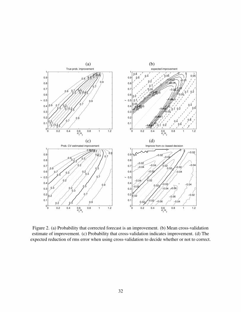
To understand better the performance of cross-validation we perform Monte Carlo simulations

12

of the correction scheme in (1), focusing on the issue of how well cross-validation estimates the

corrected forecast error, and in particular how well cross-validation identifies situations where

linear regression leads to increased error. We generate 20 years of observations and forecasts

with normally distributed errors. First, we compute the regression coefficient from the 20-year

sample and compare the rms error of the corrected and uncorrected forecasts in the population.

Figure 2a shows, as a function of correlation and variance ratio, the probability of the sample-

estimated regression coefficient producing a corrected forecast with lower rms error. Then we use

cross-validation to estimate the rms error of the corrected forecast, and Fig. 2b shows the expected

improvement as indicated by cross-validation. The cross-validation estimate indicates an increase

in rms error over a larger region of phase-space (correlation r and variance ratio) than actually

occurs (compare with Fig. 1b). This result is not surprising since the expected error variance

estimated by cross-validation is larger than the population error variance (Bunke and Droge 1984).

Comparing the cross-validation estimate of corrected forecast error with the in-sample estimate

of uncorrected forecast error provides the likelihood of cross-validation indicating an improved

forecast (Fig. 2c). Comparison of Figs. 2a and 2c shows that the likelihood of cross-validation

indicating improvement is too large near the line where a = 1 and too small away from it. This

result suggests that one cannot characterize cross-validation as being uniformly either too generous

or too strict in deciding whether or not correction gives an improvement since it may err in either

direction depending on the characteristics of the problem. The Monte Carlo simulation allows us

to compute the expected change in rms error when cross-validation is used to decide whether or not

to do linear regression relative to the strategy of always doing linear regression; linear regression

is used to correct the forecast when cross-validation indicates that it reduces rms error (Fig. 2d). In

regions of phase space where the benefit of correction is large, the impact of using cross-validation

to decide whether or not to correct is slightly negative. This finding is not unreasonable since while

the likelihood of cross-validation not indicating a reduction in rms error is slight (see Figure. 2a),

the negative impact of not correcting is large. A positive impact is seen around the line a = 1

where most of the time cross-validation will correctly indicate that linear regression increases rms

13

error.

While correction on a per gridpoint basis does not change the correlation, there is a negative

correlation bias associated with leave-one-out cross-validation that we expect to be a function of

sample size and correlation level to leading order (Barnston and van den Dool 1993). Following

Barnston and van den Dool (1993) we construct a synthetic data set with 20 samples and compute

the cross-validation bias as a function of correlation (Fig 3). For a correlation value of 0.6, the

bias is around 0.1. However, if spatially averaged correlation is the skill metric, contributions from

regions where the skill is essentially zero (and bias is greater than 0.6) may be significant. Thus,

the average bias may be more severe than that corresponding to the average correlation.

c. Pattern and local correction

The performance of univariate corrections is limited by not using information about the spatial

relations that underlie large-scale patterns like those observed in the tropical Pacific SST. Here we

use canonical correlation analysis (CCA; Appendix) to identify forecast patterns whose time-series

are correlated with those of observation patterns. EOF-prefiltering is used to reduce the number of

spatial degrees of freedom (Barnett and Preisendorfer 1987); forecast and and observed SST are

projected onto some small number of EOFs which describe large-scale structures.

The observed SST initial condition for the coupled model contains small-scale information

that may not project onto the generally large-scale EOF patterns. It is plausible that some of this

small-scale information persists in the coupled model forecast and in nature, and that because

of EOF-prefiltering is neglected in the CCA correction. It is desirable to develop a correction

that retains useful information lost in EOF-prefiltering because it explains relatively little of the

historical variance. Here we use two regressions to produce a forecast correction that behaves

like a pattern correction on the structures explained by the leading EOFs and like a gridpoint

correction otherwise. First we use CCA to develop a few sets of regression forecast and observation

patterns. The gridpoint regression is performed between the parts of the observation and forecast

14

that are spatially orthogonal and temporally uncorrelated to the large-scale patterns defined by the

EOFs. Since the data used for the CCA and for the gridpoint regression are mutually independent,

the procedure remains a least-squares estimate and there is no “double counting” of the data. A

limitation of the procedure is that is assumes no correlation between large- and small-scale errors.

4. Results

a. Domain-averaged results

We examine the performance of three correction methods: gridpoint (univariate), CCA and CCA

plus gridpoint (CCA+) applied to ECM, ECM-Ens and ICM SST predictions. Forecast starts are

limited to January and July with leads of up to six months. For example, the six leads for the

January 1 start are forecasts for January, February, . . . , June. Benchmarks are provided by two

reference forecasts: (i) a persistence forecast which consists of the observed SST anomaly from

the month preceding the forecast start added to the climatology of the verification month and

(ii) a purely statistical CCA forecast whose predictor is the observed SST anomaly of the month

preceding the forecast start. This choice of predictor for the statistical forecast is certainly not

optimal since it contains only partial information about the state and recent direction of evolution

of the coupled atmosphere ocean system (Xue et al. 2000). The statistical forecasts starting in

January use 7 EOF modes and 5 CCA modes for all leads; the forecasts starting in July use 3

EOF modes and 3 CCA modes. The number of modes is chosen to give good cross-validated skill.

The statistical forecasts are made in a leave-one-out cross-validation manner, and the monthly

SST climatology used in the persistence and statistical forecasts does not contain any of the data

being forecast. Systematic bias is removed from the uncorrected forecasts in a similar manner. The

forecast SST is the forecast anomaly with respect to the forecast climatology added to the observed

climatology where the climatologies do not include the year of the current forecast. This method

gives slightly lower skill levels compared to using all the data to compute the climatologies.

A general picture of model skill and correction performance is given by the domain-averaged

15

correlation and rms error shown in Figs. 4–6 for the for the ECM, ECM-Ens and ICM predictions

respectively. These basin-wide skill metrics are similar to, but distinct from ones based on NINO

indices. The skill of forecasts made in January tends to decrease more quickly as lead time in-

creases than do forecasts made in July, a reflection of the difficulty of making forecasts through the

so-called “spring barrier.” The average correlation of the gridpoint corrected forecasts is lower than

that of the uncorrected forecasts in all cases. To examine the extent to which this reduction in aver-

age correlation can be explained by the bias due to cross-validation, we use the bias data shown in

Fig. 3 to construct an empirical relation between correlation level and cross-validation bias. When

we add this cross-validation bias to the average correlation of the uncorrected forecasts, the sum

agrees well with the cross-validation estimated correlation in most cases; the agreement is poorest

for ICM forecasts starting in January.

Turning to the rms error of the gridpoint corrections, we see that the gridpoint corrected ECM

forecasts have lower domain-averaged rms error than the uncorrected forecasts for all leads and

both start months (Fig. 4b,d). The same is true for most of the ECM-Ens forecasts with January

starts at lead 6 and July starts at lead 1 being exceptions (Fig. 5b,d). In contrast, the gridpoint cor-

rected ICM forecasts (Fig. 6b,d) have reduced domain-averaged rms error only with leads greater

than 4 (January starts) or 3 (July starts). That is, linear regression increases the average rms error

estimated by cross-validation of ICM forecasts for shorter leads. To see if this increase in rms

error can be explained by the impact of sampling error on the regression coefficient, we plot the

rms error estimate based on sample size and in-sample error in (5). This in-sample estimate also

indicates that linear regression increases rms error, although to a lesser degree. The in-sample

estimate of the average rms error after gridpoint correction generally agrees with that given by

cross-validation.

Now looking at the CCA corrections we note that at the first lead, the CCA corrections have less

skill (lower domain-averaged correlation and higher domain-averaged rms error) than the gridpoint

corrected forecasts, in line with our expectation that information in initial conditions may provide

useful information that does not project onto patterns that can be robustly estimated. Perhaps for

16

similar reasons, the persistence forecasts have more skill (particularly average correlation) than

the purely statistical ones at the initial lead. The hybrid CCA+ method, designed to incorporate

both large- and small-scale information, performs comparably or better than either the gridpoint

or CCA, particularly at the initial leads. We expect the CCA+ corrections to have limited benefit

compared to the CCA corrections at longer leads since there is little reason to expect that the

prediction models are either able to retain or create useful information that does not project onto

the leading modes of variability of the system.

Comparison of Figs. 4 and 5 indicates the benefit that ensemble averaging has on skill, par-

ticularly rms error. We expect that using the ensemble average tends to remove SST responses

associated with unpredictable components of the coupled model, such as atmospheric noise or

“weather.” The ICM by design has a simpler atmosphere that eliminates much of this kind of in-

ternal variability. In regions where there is little SST predictability derived from initial conditions,

we expect both the ensemble average and the single-member gridpoint-corrected forecast to be

approximately zero. The ensemble average is zero because the SST is unconstrained by the initial

conditions, and the single-member gridpoint-corrected forecast is zero because it is uncorrelated

with observations. In this circumstance, the ensemble averaged forecast and regression corrected

forecast have the same rms error which is determined by climatology. However, in general, en-

semble averaging is able to enhance small predictable signals by reducing the noise due to internal

variability. The regression methods discussed here are unable to do this since the noise in a single

realization of the model (as well as noise in observations) may overwhelm the predicable com-

ponent. We notice that the rms error of the ECM-Ens forecasts starting in January is lower than

that of the gridpoint-corrected ECM forecasts, suggesting that ensemble averaging may be doing

more than simply damping forecasts where there is little skill. On the other hand, the rms error

of the ECM-Ens forecasts starting in July is roughly comparable to that of the gridpoint-corrected

ECM forecasts. Domain-averaged correlation skill also increases with ensemble averaging with the

change being largest for January starts, behavior consistent with the speculation above regarding

the different effects of ensemble averaging and gridpoint regression on rms error.

17

The persistence and purely statistical forecasts have skill levels that are not easily surpassed,

at least with the skill metrics used here that include off-equatorial regions. Uncorrected ECM

forecasts starting in January do not equal the average correlation of the persistence forecasts at

any lead time, and July forecasts match the average correlation of the persistence forecasts only

after lead 4. Uncorrected ECM forecasts have lower average rms error than persistence after leads

3 and 4 for January and July starts respectively but do not match the rms error of the purely

statistical forecasts. Gridpoint and pattern corrected ECM forecasts have lower rms error than

persistence after the first lead but higher rms error than the purely statistical forecast for January

starts; corrected and purely statistical forecast have similar rms error for July starts. Average

correlation of the uncorrected ECM-Ens forecasts matches that of persistence after leads 5 and 2

for the January and July start respectively. The rms error of the uncorrected ECM-Ens forecasts

is lower than that of persistence for almost all starts and leads (the lead 1 forecast starting in

January being the exception). Gridpoint and pattern corrections of the ECM-Ens forecasts have

slight impact on rms error for January starts; the rms error of the corrected ECM-Ens forecasts

is comparable for the July starts and matches that of the purely statistical forecast. ICM SST

forecasts made in January match the average correlation of persistence up to lead 4 but do not

match the skill of the statistical forecasts for leads 3-6. ICM forecasts starting in July surpass the

average correlation of the benchmark forecasts at all leads though the rms error is slightly higher

than that of the purely statistical forecast for leads greater than 2.

b. July forecasts of December SST

We look in more detail at the forecasts of December SST made the previous July. These forecasts

are quite skillful, and statistical corrections can use this skill to correct systematic deficiencies.

Figure 7 shows the homogeneous covariance patterns of the leading CCA mode for the ECM fore-

casts. The model pattern extends further west, is more restricted to the equator and does not extend

far enough south along the coast of South America. Differences in the model and observation

18

patterns are an indication of systematic model errors. The western extension of the coupled model

ENSO pattern is likely related to the tendency of coupled models to suffer from a double ITCZ and

too much western extension of the cold tongue, and hence too much variability in the west. The

effect of the CCA correction is to replace the model pattern in Fig. 7a with the observation pattern

in Fig. 7b. The CCA mode for the ECM-Ens forecast in Fig. 8 has smoother structure. West-

ward extension of variability is reduced but deficiencies in the structure along the South American

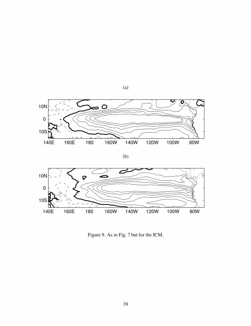
coast remain. Figure 9 shows the homogeneous covariance patterns of the leading CCA mode for

the ICM forecasts. Here the differences between the model and observation patterns are smaller,

reflecting perhaps the use of an empirical atmosphere and the empirical relation between the sub-

surface and SST. Variability along the equator does not quite extend far enough west. Similar to the

ECM and ECM-Ens forecasts, the ICM forecasts lack structure extending south along the South

American coast.

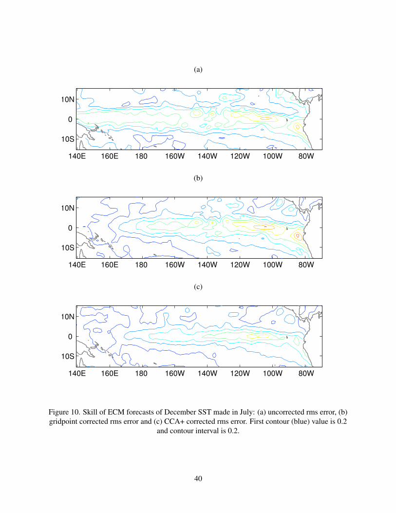
The spatial pattern of the rms error of the ECM forecasts (Fig. 10a) is consistent with the

systematic differences between model and observation CCA patterns with rms errors that extend

across the domain. Errors in the west are associated with excessive variance caused by an ENSO

pattern that extends too far west; the natural climate system appears to be sensitive to SST forcing

in this region (Barlow et al. 2002). Both the gridpoint and pattern-based CCA correction are able to

fix this deficiency; recall that regression is effective and relatively insensitive to sample size when

damping variance that is too large. The grid point correction has less success in reducing error

levels in the eastern part of the domain; in fact, rms error levels there rise slightly. On the other

hand, pattern-based CCA corrections (not shown) use spatial relationships and are able to reduce

the rms level of systematic errors in the east. The CCA+ correction (4 EOFs and 4 CCA modes;

Fig. 10c) has similar overall performance and reduces error variance in both regions. Highest

correlations of the ECM forecasts with observations are found in the central part of the domain

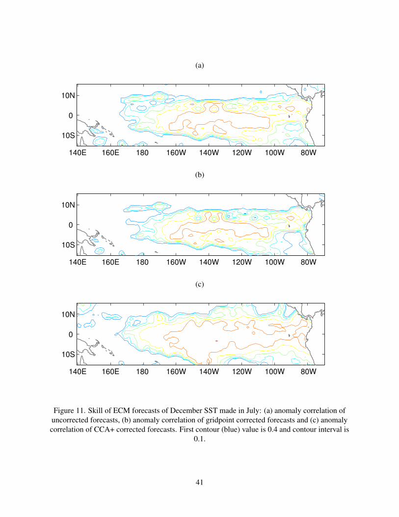
and are mostly restricted to the equator (Fig. 11a). The cross-validation estimate of the anomaly

correlation of the gridpoint correction has lower values due to the bias of the procedure, though

the pattern of correlation is similar. The pattern-based CCA+ method increases the spatial extent

19

and the values of high anomaly correlation skill.

Ensemble averaging reduces the western extent of rms error in ECM-Ens forecasts (Fig12a),

and overall error levels of the uncorrected ECM-Ens forecast are comparable to those of the grid-

point corrected ECM forecast. Gridpoint and pattern corrections slightly reduce rms error further

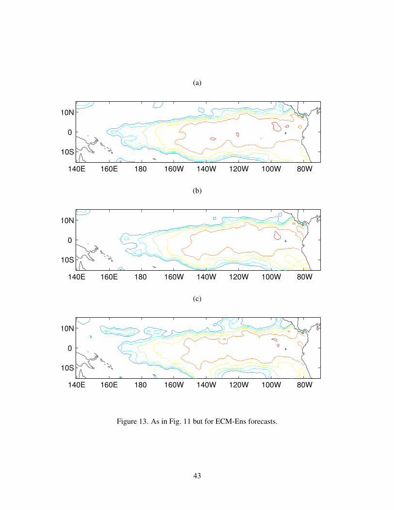
with some benefit in the eastern part of the domain. The ECM-Ens forecasts have correlation

exceeding 0.8 in a large domain, and correction does not lead to improvement (Fig. 13).

Gridpoint correction reduces the overall error level of the ICM forecasts, although there is an

increase in rms error in the extreme eastern part of the domain (Fig. 14a,b). The CCA+ correction

gives additional reduction in domain-averaged rms error, including and in the east (5 EOFs and

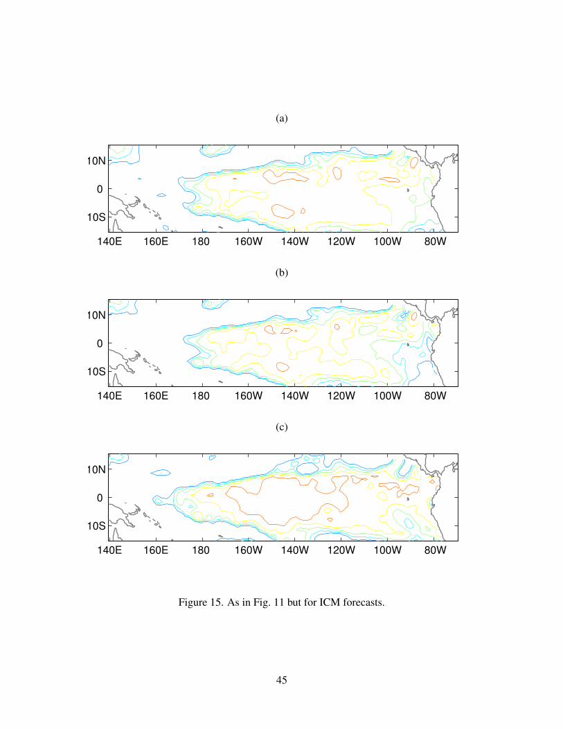
3 CCA modes; Fig14c). Figure 15 shows that the anomaly correlation of the ICM forecasts with

observations are above 0.7 for much of the domain. The cross-validated estimate of anomaly

correlation for the gridpoint corrected forecasts has slightly lower values. The CCA+ correction

has a positive impact on the basin-averaged correlation and increases correlation values in the

central Pacific to over 0.8.

5. Summary and conclusions

Dynamical prediction of SST, a critical part of any short-term climate forecasting system, requires

the use of dynamical models that generally have systematic errors. This paper is concerned with

the statistical correction of such errors using linear regression approaches. The short histories of

model forecasts, whether real-time or retrospective, are a source of difficulty when developing

regression-based corrections. The roles of sample size, existing level of predictive skill, and level

of existing systematic error in the uncorrected predictions are examined in evaluating the potential

benefit of a linear correction. In this study we have not treated mean biases, as it is assumed that

these can be easily accounted for. Thus the study begins with departures from the means of the

respective observed and model data sets.

In an idealized scalar example (section 3), the next order of systematic linear error correction

20

involves forecast amplitude. With small samples such as the typical 20 years of model SST fore-

cast data available, corrections tend to be beneficial only when there are substantial deviations in

amplitude from that called for by the forecast versus observation correlation. To minimize squared

errors, forecasts having low skill (e.g. low temporal correlation and high root-mean-squared error)

should be damped so as to have relatively low amplitude as compared with higher skill forecasts.

The closer the amplitude of the uncorrected forecasts is to the squared error-minimizing ampli-

tude dictated by the skill, the less likely is the correction to improve the skill. This results from a

combination of there being less ”room for improvement”, and the sampling error in the amplitude-

determining regression coefficient underlying the correction: the smaller the sample size, the more

likely and larger is the sampling error in the estimate of the coefficient. Larger samples would

enable the initial amplitude to be closer to optimum and still benefit from a correction.

Extension to the multivariate (CCA) level and application to three dynamical SST prediction

models enabled demonstrations of improvement in the skills of tropical Pacific SST forecasts both

during times of the year when such forecasts are easier as well as more difficult. Pattern corrections

are seen to reduce marked systematic errors in pattern structure that are well within the reach of

the correction equations based on as little as 20 years of model versus observed data. To further

refine the correction process, individual scalar corrections on a per-gridpoint basis are applied in

addition and orthogonally to the CCA corrections, and are found to further increase the skill of

mainly the shortest lead predictions. This local component of the correction treats SST anomalies

of smaller spatial scale that do not project onto the CCA modes and are generally associated with

the persistence of features in the initial conditions.

In this study we also have the opportunity to compare the effects of statistical correction with

ensemble averaging. Both methods attempt to remove unpredictable noise. While both procedures

should be successful at damping unpredictable components, ensemble averaging is able, in addi-

tion, to amplify relatively small predictable signals and reduce noise. Other statistical methods

have the potential to achieve such “filtering” in the multivariate setting to the extent that signal and

noise can be separated (Allen and Smith 1997; Chang et al. 2000). Here we note that while statisti-

21

cal corrections of single member SST forecasts made in July have comparable skill to uncorrected

ensemble averages, the skill of statistically corrected forecasts made in January do not match the

skill of the ensemble averaged forecasts.

In summary, regression-based corrections to SST predictions by dynamical models are found

to be capable of making the dynamical predictions more skillful and useful until such time that the

models become freer of systematic errors. The same conclusion applies equally to AGCM predic-

tions of atmospheric climate (e.g., Tippett et al. 2005). Of relevance is that the failure of dynamical

approaches to outperform purely statistical SST prediction models (Barnston et al. 1999) is partly

attributable to the fact that the latter automatically correct systematic errors. Statistical correction

of dynamical SST predictions would be expected to increase their standing relative to the purely

statistical prediction methods.

Acknowledgements. Comments and suggestions from Andrew Robertson and Steve Zebiak im-

proved the quality of this paper. We thank Benno Blumenthal for the IRI Data Library. IRI is

supported by its sponsors and NOAA Office of Global Programs Grant number NA07GP0213.

22

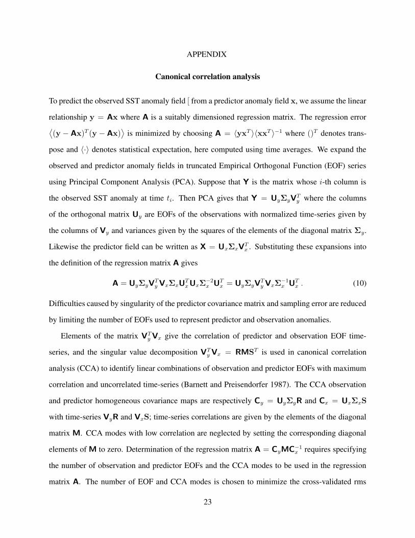
APPENDIX

Canonical correlation analysis

To predict the observed SST anomaly field [ from a predictor anomaly field x, we assume the linear

relationship y = Ax where A is a suitably dimensioned regression matrix. The regression error⟨

(y − Ax)T (y − Ax)⟩

is minimized by choosing A = 〈yxT 〉〈xxT 〉−1 where ()T denotes trans-

pose and 〈·〉 denotes statistical expectation, here computed using time averages. We expand the

observed and predictor anomaly fields in truncated Empirical Orthogonal Function (EOF) series

using Principal Component Analysis (PCA). Suppose that Y is the matrix whose i-th column is

the observed SST anomaly at time ti. Then PCA gives that Y = UyΣyVTy where the columns

of the orthogonal matrix Uy are EOFs of the observations with normalized time-series given by

the columns of Vy and variances given by the squares of the elements of the diagonal matrix Σy.

Likewise the predictor field can be written as X = UxΣxVTx . Substituting these expansions into

the definition of the regression matrix A gives

A = UyΣyVTy VxΣxU

Tx UxΣ

−2

x UTx = UyΣyV

Ty VxΣ

−1

x UTx . (10)

Difficulties caused by singularity of the predictor covariance matrix and sampling error are reduced

by limiting the number of EOFs used to represent predictor and observation anomalies.

Elements of the matrix VTy Vx give the correlation of predictor and observation EOF time-

series, and the singular value decomposition VTy Vx = RMST is used in canonical correlation

analysis (CCA) to identify linear combinations of observation and predictor EOFs with maximum

correlation and uncorrelated time-series (Barnett and Preisendorfer 1987). The CCA observation

and predictor homogeneous covariance maps are respectively Cy = UyΣyR and Cx = UxΣxS

with time-series VyR and VxS; time-series correlations are given by the elements of the diagonal

matrix M. CCA modes with low correlation are neglected by setting the corresponding diagonal

elements of M to zero. Determination of the regression matrix A = CyMC−1

x requires specifying

the number of observation and predictor EOFs and the CCA modes to be used in the regression

matrix A. The number of EOF and CCA modes is chosen to minimize the cross-validated rms

23

error. Climatologies and EOFs are re-computed at each iteration of the cross-validation, and we

restrict the number of observation EOFs and forecast EOFs to be equal. The number of modes

generally depends on forecast start month and lead. If a CCA mode is discarded, all CCA modes

with lower correlation are also discarded.

24

REFERENCES

Allen, M. R., and L. A. Smith, 1997: Optimal filtering in singular spectrum analysis. Phys. Lett.,

234, 419–428.

Barlow, M., H. Cullen, and B. Lyon, 2002: Drought in central and southwest Asia: La Nina, the

warm pool, and Indian ocean precipitation. J. Climate, 15, 697–700.

Barnett, T. P., 1981: Statistical prediction of North American air temperatures from Pacific predic-

tions. Mon. Wea. Rev., 109, 1021–1041.

Barnett, T. P., and R. Preisendorfer, 1987: Origins and levels of monthly and seasonal forecast

skill for United States surface air temperatures determined by canonical correlation analysis.

Mon. Wea. Rev., 115, 1825–1850.

Barnston, A. G., 1994: Linear statistical short-term climate predictive skill in the Northern Hemi-

sphere. J. Climate, 7, 1513–1564.

Barnston, A. G., and H. M. van den Dool, 1993: A degeneracy in cross-validated skill in

regression-based forecasts. J. Climate, 6, 963–977.

Barnston, A. G., M. H. Glantz, and Y. He, 1999: Predictive skill of statistical and dynamical

climate models in SST forecasts during the 1997-98 El Nino Episode and the 1998 La Nina

Onse. Bull. Am. Meteor. Soc., 80, 217–243.

Bengtsson, L., U. Schlese, E. Roeckner, M. Latif, T. Barnett, and N. Graham, 1993: A two tiered

approach to long-range climate forecasting. Science, 261, 1026–1029.

Bunke, O., and B. Droge, 1984: Boostrap and cross-validation estimates of the prediction error for

linear regresion models. Ann. Statist., 12, 1400–1424.

25

Chang, P., R. Saravanan, L. Ji, and G. C. Hegerl, 2000: The effect of local sea surface temperatures

on atmospheric circulation over the tropical atlantic sector. J. Climate, 13, 2195–2216.

Derber, J., and A. Rosati, 1989: A global oceanic data assimilation system. J. Phys. Oceanogr., 9,

1333–1347.

DeWitt, D. G., 2004: Retrospective forecasts of interannual sea surface temperature anomalies

from 1982 to present using a directly coupled atmosphere-ocean general circulation model.

Mon. Wea. Rev. submitted.

Fedorov, A. V., S. Harper, S. Philander, B. Winter, and A. Wittenberg, 2003: How predictable is

El Nino? Bull. Amer. Met. Soc., 84, 911–919.

Goddard, L., S. J. Mason, S. E. Zebiak, C. F. Ropelewski, R. Basher, and M. A. Cane, 2001:

Current approaches to seasonal-to-interannual climate prediction. Int. J. Climatol., 21, 1111–

1152.

Gong, X., A. G. Barnston, and M. N. Ward, 2003: The effect of spatial aggregation on the skill of

seasonal precipitation forecasts. J. Climate, 18, 3059–3071.

Horel, J. D., and J. M. Wallace, 1981: Planetary-scale atmospheric phenomena associated with the

Southern Oscillation. Mon. Wea. Rev., 109, 813–829.

Ji, M., A. Kumar, and A. Leetma, 1994: A multiseason climate forecast system at the National

Meteorological Center. Bull. Am. Meteor. Soc., 75, 569–577.

Keenlyside, N., and R. Kleeman, 2002: On the annual cycle of the zonal currents in the equatorial

pacific. J. Geophys. Res., 107. doi:10.1029/2000JC0007111.

Kirtman, B. P., 2003: The COLA anomaly coupled model: Ensemble ENSO prediction.

Mon. Wea. Rev., 131, 2324–2341.

26

Landman, W. A., and S. J. Mason, 2001: Forecasts of near-global sea surface temperatures using

canonical correlation analysis. J. Climate, 14, 3819–3833.

Livezey, R. E., 1990: Variability of skill of long-range forecasts and implications for their use and

value. Bull. Am. Meteor. Soc., 71, 300–309.

Mason, S. J., L. Goddard, N. E. Graham, E. Yulaeva, L. Sun, and P. A. Arkin, 1999: The IRI

seasonal climate prediction system and the 1997/98 El Nino. Bull. Am. Meteor. Soc., 80, 1853–

1873.

McCreary, J. P., 1981: A linear stratified ocean model of the equatorial undercurrent. Phil. Trans.

Roy. Soc, A298, 603–635.

Metzger, S., M. Latif, and K. Fraedrich, 2004: Combining ENSO forecasts: A feasibility study.

Mon. Wea. Rev., 132, 456–472.

Michaelsen, J., 1987: Cross-validation in statistical climate forecast models. J. Climate Appl.

Meteor., 26, 1589–1600.

Montgomery, D. C., and E. A. Peck, 1992: Introduction to linear regression analysis. Wiley series

in probability and mathematical statistics, 2nd edition. John Wiley and Sons, New York.

Pacanowski, R. C., and S. M. Griffies, 1998: MOM 3.0 Manual. NOAA/Geophysical Fluid Dy-

namics Laboratory, Princeton, NJ.

Reynolds, R. W., N. A. Rayner, T. M. Smith, D. C. Stokes, and W. Wang, 2002: An improved in

situ and satellite SST analysis for climate. J. Climate, 15, 1609–1625.

Roeckner, E., K. Arpe, L. Bengtsson, M. Christoph, M. Claussen, L. Dumenil, M. Esch, M. Gior-

getta, U. Schlese, and U. Schulzweida, 1996: The atmospheric general circulation model

ECHAM-4: Model description and simulation of present-day climate. Technical Report 218,

Max-Planck Institute for Meteorology, Hamburg, Germany. 90 pp.

27

Ropelewski, C., and M. Halpert, 1987: Global and regional scale precipitation patterns associated

with the El Nino/Southern Oscillation. Mon. Wea. Rev., 115, 1606–1626.

Saha, S., W. Wang, H.-L. Pan, D. Behringer, S. Nadiga, S. Moorthi, and S. Harper, 2003: Hindcast

skill in SST prediction in the new NCEP coupled atmosphere-ocean model. In 28th Annual

Climate Diagnostics and Prediction Workshop. Reno Nevada.

Schneider, E. K., D. G. DeWitt, A. Rosati, B. P. Kirtman, L. Ji, and J. J. Tribbia, 2003: Retrospec-

tive ENSO forecasts: Sensitivity to atmospheric model and ocean resolution. Mon. Wea. Rev.,

131, 3038–3060.

Shao, J., 1993: Linear model selection by cross-validation. Journal of the American Statistical

Association, 88, 486–494.

Shukla, J., 1998: Predictability in the midst of chaos: A scientific basis for climate forecasting.

Science, 282, 728–731.

Stockdale, T. N., D. L. T. Anderson, J. O. S. Alves, and M. A. Balmaseda, 1998: Global seasonal

rainfall forecasts using a coupled ocean-atmosphere model. Nature, 392, 370–373.

Terray, L., A. Piacentini, and S. Valcke, 1999: ASIS 2.3, Ocean Atmosphere Sea Ice Soil: User’s

guide. Technical Report TR/CMGC/99/37, CERFACS, Toulouse, France. [Available online at

http://www.cerfacs.fr/globc/publication.html].

Tippett, M. K., L. Goddard, and A. G. Barnston, 2005: Statistical-Dynamical Seasonal Forecasts

of Central Southwest Asia winter precipitation. J. Climate. accepted.

Xue, Y. A., A. Leetma, and M. Ji, 2000: ENSO predictions with Markov models: The impact of

sea level. J. Climate, 13, 849–871.

Zebiak, S. E., and M. A. Cane, 1987: A model El Nino-Southern Oscillation. Mon. Wea. Rev., 115,

2262–2278.

28

Zhang, R., S. E. Zebiak, R. Kleeman, and N. Keenlyside, 2003: A new intermediate

coupled model for El Nino simulation and prediction. Geophys. Res. Lett., 30, 2112.

doi:10.1029/2003GL018010.

Zhang, R.-H., S. E. Zebiak, R. Kleeman, and N. Keenlyside, 2004: Retrospective El Nino hind-

cast/forecast using an improved intermediate coupled model. Mon. Wea. Rev. submitted.

29

List of Figures

1 (a) Contours of sample size n resulting in expected variance improvement of zero.(b) Expected variance improvement for n = 20. Positive values are dashed. (c)Contours of 10th percentile of expected improvement for n = 20; only negativevalues are shown. The dotted line in all plots is the line r = σx/σy. The regressioncoefficient a is greater than unity above this line and and less than unity below it. . 31

2 (a) Probability that corrected forecast is an improvement. (b) Mean cross-validationestimate of improvement. (c) Probability that cross-validation indicates improve-ment. (d) The expected reduction of rms error when using cross-validation todecide whether or not to correct. . . . . . . . . . . . . . . . . . . . . . . . . . . . 32

3 Bias of the correlation estimated by cross-validation with sample size 20. . . . . . 334 Domain-averaged (a) correlation and (b) rms error for ECM forecasts starting in

January as a function of lead-time. Domain-averaged (c) correlation and (d) rmserror for ECM forecasts starting in July as a function of lead-time. Different curvesdenote results for for uncorrected (filled circles), gridpoint (solid line, plus sign),estimated gridpoint (dashed line line, plus sign), CCA (solid line, squares), CCA+(dashed lines, squares), persistence (dashed line, x’s), statistical (solid line, x’s). . 34

5 As in Fig. 4 but for ECM-Ens forecasts. . . . . . . . . . . . . . . . . . . . . . . . 356 As in Fig. 4 but for ICM forecasts. . . . . . . . . . . . . . . . . . . . . . . . . . . 367 Homogeneous covariance patterns (unitless; same contour interval) of the lead-

ing mode obtained from CCA between (a) observed December SST and (b) ECMforecast (July starts). A thick line marks the zero contour. . . . . . . . . . . . . . . 37

8 As in Fig. 7 but for the ECM-Ens. . . . . . . . . . . . . . . . . . . . . . . . . . . 389 As in Fig. 7 but for the ICM. . . . . . . . . . . . . . . . . . . . . . . . . . . . . . 3910 Skill of ECM forecasts of December SST made in July: (a) uncorrected rms error,

(b) gridpoint corrected rms error and (c) CCA+ corrected rms error. First contour(blue) value is 0.2 and contour interval is 0.2. . . . . . . . . . . . . . . . . . . . . 40

11 Skill of ECM forecasts of December SST made in July: (a) anomaly correlation ofuncorrected forecasts, (b) anomaly correlation of gridpoint corrected forecasts and(c) anomaly correlation of CCA+ corrected forecasts. First contour (blue) value is0.4 and contour interval is 0.1. . . . . . . . . . . . . . . . . . . . . . . . . . . . . 41

12 As in Fig. 10 but for ECM-Ens forecasts. . . . . . . . . . . . . . . . . . . . . . . 4213 As in Fig. 11 but for ECM-Ens forecasts. . . . . . . . . . . . . . . . . . . . . . . 4314 As in Fig. 10 but for ICM forecasts. . . . . . . . . . . . . . . . . . . . . . . . . . 4415 As in Fig. 11 but for ICM forecasts. . . . . . . . . . . . . . . . . . . . . . . . . . 45

30

(a) (b) (c)

0 0.2 0.4 0.6 0.8 1 1.20

0.1

0.2

0.3

0.4

0.5

0.6

0.7

0.8

0.9

1

σx/σ

y

r

10

20

50100

102050

100

a=1

0 0.2 0.4 0.6 0.8 1 1.20

0.1

0.2

0.3

0.4

0.5

0.6

0.7

0.8

0.9

1

σx/σ

y

r

1

0.8

0.6

0.4

0.2

0.1

0.05

−0.04

−0.03

−0.02

−0.01

00.8

0.6

0.4

0.2

0.10.05

0 0.2 0.4 0.6 0.8 1 1.20

0.1

0.2

0.3

0.4

0.5

0.6

0.7

0.8

0.9

1

σx/σ

y

r

−0.08

−0.06

−0.04

−0.02

0

Figure 1. (a) Contours of sample size n resulting in expected variance improvement of zero. (b)Expected variance improvement for n = 20. Positive values are dashed. (c) Contours of 10th

percentile of expected improvement for n = 20; only negative values are shown. The dotted linein all plots is the line r = σx/σy. The regression coefficient a is greater than unity above this line

and and less than unity below it.

31

(a) (b)

0 0.2 0.4 0.6 0.8 1 1.20

0.1

0.2

0.3

0.4

0.5

0.6

0.7

0.8

0.9

1

σx/σ

y

r

True prob. improvement

0.1

0.1

0.1

0.1

0.1

0.1

0.1 0.3

0.3

0.3

0.30.3

0.3

0.3

0.3

0.5

0.5

0.5

0.50.5

0.5

0.5

0.7

0.7

0.7

0.7

0.7

0.7

0.9

0.9

0.90.9

0.9

0.9

0 0.2 0.4 0.6 0.8 1 1.20

0.1

0.2

0.3

0.4

0.5

0.6

0.7

0.8

0.9

1

σx/σ

y

r

expected improvement

−0.05

−0.05

−0.05−0.05

−0.05

−0.04

−0.04

−0.04

−0.04

−0.04

−0.03

−0.03

−0.03

−0.03

−0.03

−0.03

−0.02

−0.02

−0.02

−0.02

−0.02

−0.02

−0.01

−0.01

−0.01−0.01

−0.01

−0.01

0

0

0

00

0

0

0.05

0.05

0.050.05

0.05

0.05

0.1

0.1

0.1

0.1

0.1

0.2

0.2

0.2

0.2

0.2

0.4

0.4

0.4

0.6

0.6

0.6

0.8

0.8

1

(c) (d)

0 0.2 0.4 0.6 0.8 1 1.20

0.1

0.2

0.3

0.4

0.5

0.6

0.7

0.8

0.9

1

σx/σ

y

r

Prob. CV estimated improvement

0.2

0.2

0.2

0.20.2

0.2

0.2

0.2

0.3

0.3

0.30.3

0.3

0.3

0.5

0.5

0.5

0.5

0.5

0.5

0.7

0.7

0.7

0.7

0.7

0.7

0.9

0.9

0.9

0.9

0.9

0.9

0 0.2 0.4 0.6 0.8 1 1.20

0.1

0.2

0.3

0.4

0.5

0.6

0.7

0.8

0.9

1

σx/σ

y

r

Improve from cv−based decision

−0.06

−0.06

−0.06

−0.04

−0.04

−0.04

−0.04

−0.04

−0.04−0.04

−0.04

−0.02

−0.02

−0.02

−0.02

−0.02

−0.02

−0.02−0.02

−0.02

−0.02

0

0

0

000

0

0

0

0

0

0.02

0.02

0.020.02

0.02

0.02

Figure 2. (a) Probability that corrected forecast is an improvement. (b) Mean cross-validationestimate of improvement. (c) Probability that cross-validation indicates improvement. (d) The

expected reduction of rms error when using cross-validation to decide whether or not to correct.

32

0 0.2 0.4 0.6 0.8 1−0.9

−0.8

−0.7

−0.6

−0.5

−0.4

−0.3

−0.2

−0.1

correlation

corr

elat

ion

bias

Figure 3. Bias of the correlation estimated by cross-validation with sample size 20.

33

(a) (b)

2 4 6

0

0.2

0.4

0.6

0.8

corr

elat

ion

lead month

Jan

2 4 60.3

0.4

0.5

0.6

0.7

0.8

rms

lead month

Jan

(c) (d)

2 4 6

0

0.2

0.4

0.6

0.8

corr

elat

ion

lead month

Jul

2 4 60.3

0.4

0.5

0.6

0.7

0.8

rms

lead month

Jul

Figure 4. Domain-averaged (a) correlation and (b) rms error for ECM forecasts starting inJanuary as a function of lead-time. Domain-averaged (c) correlation and (d) rms error for ECM

forecasts starting in July as a function of lead-time. Different curves denote results for foruncorrected (filled circles), gridpoint (solid line, plus sign), estimated gridpoint (dashed line line,

plus sign), CCA (solid line, squares), CCA+ (dashed lines, squares), persistence (dashed line,x’s), statistical (solid line, x’s).

34

(a) (b)

2 4 6

0

0.2

0.4

0.6

0.8

corr

elat

ion

lead month

Jan

2 4 60.3

0.4

0.5

0.6

0.7

0.8

rms

lead month

Jan

(c) (d)

2 4 6

0

0.2

0.4

0.6

0.8

corr

elat

ion

lead month

Jul

2 4 60.3

0.4

0.5

0.6

0.7

0.8

rms

lead month

Jul

Figure 5. As in Fig. 4 but for ECM-Ens forecasts.

35

(a) (b)

2 4 6

0

0.2

0.4

0.6

0.8

corr

elat

ion

lead month

Jan

2 4 60.3

0.4

0.5

0.6

0.7

0.8

rms

lead month

Jan

(c) (d)

2 4 6

0

0.2

0.4

0.6

0.8

corr

elat

ion

lead month

Jul

2 4 60.3

0.4

0.5

0.6

0.7

0.8

rms

lead month

Jul

Figure 6. As in Fig. 4 but for ICM forecasts.

36

(a)

140E 160E 180 160W 140W 120W 100W 80W

10S

0

10N

(b)

140E 160E 180 160W 140W 120W 100W 80W

10S

0

10N

Figure 7. Homogeneous covariance patterns (unitless; same contour interval) of the leading modeobtained from CCA between (a) observed December SST and (b) ECM forecast (July starts). A

thick line marks the zero contour.

37

(a)

140E 160E 180 160W 140W 120W 100W 80W

10S

0

10N

(b)

140E 160E 180 160W 140W 120W 100W 80W

10S

0

10N

Figure 8. As in Fig. 7 but for the ECM-Ens.

38

(a)

140E 160E 180 160W 140W 120W 100W 80W

10S

0

10N

(b)

140E 160E 180 160W 140W 120W 100W 80W

10S

0

10N

Figure 9. As in Fig. 7 but for the ICM.

39

(a)

140E 160E 180 160W 140W 120W 100W 80W

10S

0

10N

(b)

140E 160E 180 160W 140W 120W 100W 80W

10S

0

10N

(c)

140E 160E 180 160W 140W 120W 100W 80W

10S

0

10N

Figure 10. Skill of ECM forecasts of December SST made in July: (a) uncorrected rms error, (b)gridpoint corrected rms error and (c) CCA+ corrected rms error. First contour (blue) value is 0.2

and contour interval is 0.2.

40

(a)

140E 160E 180 160W 140W 120W 100W 80W

10S

0

10N

(b)

140E 160E 180 160W 140W 120W 100W 80W

10S

0

10N

(c)

140E 160E 180 160W 140W 120W 100W 80W

10S

0

10N

Figure 11. Skill of ECM forecasts of December SST made in July: (a) anomaly correlation ofuncorrected forecasts, (b) anomaly correlation of gridpoint corrected forecasts and (c) anomalycorrelation of CCA+ corrected forecasts. First contour (blue) value is 0.4 and contour interval is

0.1.

41

(a)

140E 160E 180 160W 140W 120W 100W 80W

10S

0

10N

(b)

140E 160E 180 160W 140W 120W 100W 80W

10S

0

10N

(c)

140E 160E 180 160W 140W 120W 100W 80W

10S

0

10N

Figure 12. As in Fig. 10 but for ECM-Ens forecasts.

42

(a)

140E 160E 180 160W 140W 120W 100W 80W

10S

0

10N

(b)

140E 160E 180 160W 140W 120W 100W 80W

10S

0

10N

(c)

140E 160E 180 160W 140W 120W 100W 80W

10S

0

10N

Figure 13. As in Fig. 11 but for ECM-Ens forecasts.

43

(a)

140E 160E 180 160W 140W 120W 100W 80W

10S

0

10N

(b)

140E 160E 180 160W 140W 120W 100W 80W

10S

0

10N

(c)

140E 160E 180 160W 140W 120W 100W 80W

10S

0

10N

Figure 14. As in Fig. 10 but for ICM forecasts.

44

(a)

140E 160E 180 160W 140W 120W 100W 80W

10S

0

10N

(b)

140E 160E 180 160W 140W 120W 100W 80W

10S

0

10N

(c)

140E 160E 180 160W 140W 120W 100W 80W

10S

0

10N

Figure 15. As in Fig. 11 but for ICM forecasts.

45