Virtual University of PakistanLecture No. 11

Statistics and Probability

by

Miss Saleha Naghmi Habibullah

IN THE LAST LECTURE, YOU LEARNT

• Concept of dispersion• Absolute measures of dispersion• Relative measures of dispersion• Range • Coefficient of dispersion• Quartile Deviation• Coefficient of Quartile Deviation

TOPICS FOR TODAY

• Mean Deviation• Standard Deviation and Variance• Coefficient of variation

The first thing to note is that, whereas the range as well as the quartile deviation are two such measures of dispersion which are NOT based on all the values, the mean deviation and the standard deviation are two such measures of dispersion that involve each and every data-value in their computation.

You must have noted that the range was measuring the dispersion of the data-set around the mid-range, whereas the quartile deviation was measuring the dispersion of the data-set around the median.

How are we to decide upon the amount of dispersion round the arithmetic mean? It would seem reasonable to compute the DISTANCE of each observed value in the series from the arithmetic mean of the series.

Example Example The Number of Fatalities in Motorway

Accidents in one Week:

Day Number of fatalities X

Sunday 4 Monday 6 Tuesday 2 Wednesday 0 Thursday 3 Friday 5 Saturday 8

Total 28

The arithmetic mean number of fatalities per day is:

4728

nXX

In order to determine the distances of the data-values from the mean, we subtract our value of the arithmetic mean from each daily figure, and this gives us the deviations that occur in the third column of the table below:

D a y N u m b e r o f f a t a l i t i e sX XX

S u n d a y 4 0M o n d a y 6 + 2T u e s d a y 2 – 2W e d n e s d a y 0 – 4T h u r s d a y 3 – 1F r i d a y 5 + 1S a t u r d a y 8 + 4

T O T A L 2 8 0The deviations are negative when the daily figure is less than the mean (4 accidents) and positive when the figure is higher than the mean.

It does seem, however, that our efforts for computing the dispersion of this data set have been in vain, for we find that the total amount of dispersion obtained by summing the (x – x) column comes out to be zero!

In fact, this should be no surprise, for it is a basic property of the arithmetic mean that:

The sum of the deviations of the values from the mean is zero.

The question arises, How will we measure the dispersion that is actually present in our data-set?Let us denote these absolute differences by ‘modulus of d’ or ‘mod d’.

This is evident from the third column of the table below: X X –X = d | d |

4 0 06 2 22 –2 20 –4 43 –1 15 1 18 4 4

Total 14

By ignoring the sign of the deviations we have achieved a non-zero sum in our second column. Averaging these absolute differences, we obtain a measure of dispersion known as the mean deviation.

In other words, the mean deviation is given by the formula:

n|d|.D.M i

Applying this formula in our example, we find that, the mean deviation of the number of fatalities is:

.27

14.D.M

The formula that we have just considered is valid in the case of raw data.

In case of grouped data i.e. a frequency distribution, the formula becomes:

ndf

nxxf

.D.M iiii

As far as the graphical representation of the mean deviation is concerned, it can be depicted by a horizontal line segment drawn below the X-axis on the graph of the frequency distribution, as shown below:

X

f

Mean DeviationX

Mean deviation is an absolute measure of dispersion. Its relative measure, known as the co-efficient of mean deviation, is obtained by dividing the mean deviation by the average used in the calculation of deviations i.e. the arithmetic mean. Thus

Co-efficient of M.D.Mean

.D.M

Sometimes, the mean deviation is computed by averaging the absolute deviations of the data-values from the median i.e.

nx~x

deviationMean

In such a situation, the coefficient of mean deviation is given by:

Co-efficient of M.D.Median

.D.M

In order to compute the standard deviation, rather than taking the absolute values of the deviations, we square the deviations.

Averaging these squared deviations, we obtain a statistic that is known as the variance.

Variance nxx

2

Variance Variance

The sum of squares of the deviationsThe sum of squares of the deviationsof the X from the mean, divided by theof the X from the mean, divided by theno. of values. no. of values.

Variance 2x xn

Standard DeviationStandard Deviation

2x xS

n

Let us compute these quantities for the data of the above example. Our X-values were:

X4620358

Taking the deviations of the X-values from their mean, and then squaring these deviations, we obtain:

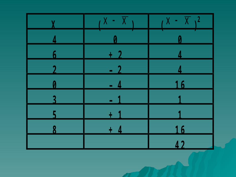
X ( xx ) ( xx ) 2

4 0 06 + 2 42 – 2 40 – 4 1 63 – 1 15 + 1 18 + 4 1 6

4 2

Obviously, both (– 2)2 and (2)2 equal 4, both (– 4)2 and (4)2 equal 16, and both (– 1)2 and (1)2 = 1.

Hence (x – x)2 = 42 is now positive, and this positive value has been achieved without ‘bending’ the rules of mathematics.

Averaging these squared deviations, the variance is given by:

n

xx 2

6742

Variance =

The variance is frequently employed in statistical work, but it should be noted that the figure achieved is in ‘squared’ units of measurement.

In the example that we have just considered, the variance has come out to be “6 squared fatalities”, which does not seem to make much sense!

In order to obtain an answer which is in the original unit of measurement, we take the positive square root of the variance. The result is known as the standard deviation.

n

xxS2

so that the standard deviation number of fatalities is:

45.2742

STANDARD DEVIATION

Hence, in this example, our standard deviation has come out to be 2.45 fatalities.

In computing the standard deviation (or variance) it can be tedious to first ascertain the arithmetic mean of a series, then subtract it from each value of the variable in the series, and finally to square each deviation and then sum.

It is very much more straight-forward to use the short cut formula given below:

22

nx

nxS

In order to apply the short cut formula, we require only the aggregate of the series (x) and the aggregate of the squares of the individual values in the series (x2). In other words, only two columns of figures are called for. The number of individual calculations is also considerably reduced, as seen below:

X X2

4 166 362 40 03 95 258 64

Total 28 154

fatalities45.26

1622728

7154S

2

Therefore

The formulae that we have just discussed are valid in case of raw data.

In case of grouped data i.e. a frequency distribution, each squared deviation round the mean must be multiplied by the appropriate frequency figure i.e.

n

xxfS2

And the short cut formula in case of a frequency distribution is:

22

nfx

nfxS

which is again preferred from the computational standpoint.

For example, the standard deviation life of a batch of electric light bulbs would be calculated as follows:

Life (inHundredsof Hours)

No. ofBulbs

f

Mid-point

xfx fx2

0 – 5 4 2.5 10.0 25.05 – 10 9 7.5 67.5 506.2510 – 20 38 15.0 570.0 8550.020 – 40 33 30.0 990.0 29700.0

40 and over 16 50.0 800.0 40000.0100 2437.5 78781.25

EXAMPLE

Therefore, standard deviation:

2

1005.2437

10025.78781S

= 13.9 hundred hours= 1390 hours

As far as the graphical representation of the standard deviation is concerned, a horizontal line segment is drawn below the X-axis on the graph of the frequency distribution --- just as in the case of the mean deviation.

X

f

Standard deviationX

The standard deviation is an absolute measure of dispersion. Its relative measure called coefficient of standard deviation is defined as:

Coefficient of S.D. MeanDeviationdardtanS

And, multiplying this quantity by 100, we obtain a very important and well-known measure called the coefficient of variation.

100XS.V.C

For example, if a comparison between the variability of distributions with different variables is required, or when we need to compare the dispersion of distributions with the same variable but with very different arithmetic means.

To illustrate the usefulness of the coefficient of variation, let us consider the following two examples:

Suppose that, in a particular year, the mean weekly earnings of skilled factory workers in one particular country were $ 19.50 with a standard deviation of $ 4, while for its neighboring country the figures were Rs. 75 and Rs. 28 respectively.

From these figures, it is not immediately apparent which country has the GREATER VARIABILITY in earnings.

The coefficient of variation quickly provides the answer:

EXAMPLE-1

COEFFICIENT OF VARIATION

For country No. 1:

5.201005.19

4 per cent,

and for country No. 2:

3.371007528

per cent.

EXAMPLE-2

The crop yield from 20 one-acre plots of wheat-land cultivated by ordinary methods averages 35 bushels with a standard deviation of 10 bushels.

The yield from similar land treated with a new fertilizer averages 58 bushels, also with a standard deviation of 10 bushels. At first glance, the yield variability may seem to be the same, but in fact it has improved (i.e. decreased) in view of the higher average to which it relates.

Again, the coefficient of variation shows this very clearly:

U n t r e a t e d l a n d :

57.281003510

p e r c e n t

T r e a t e d l a n d :

24.171005810

p e r c e n t

Coefficient of Variation:

IN TODAY’S LECTURE, YOU LEARNT

•Mean Deviation•Coefficient of Mean Deviation•Standard Deviation and Variance•Coefficient of variation

IN THE NEXT LECTURE, YOU WILL LEARN

•Chebychev’s Inequality•The Empirical Rule •The Five-Number Summary•Box and Whisker Plot