SPATIO–TEMPORAL MODELLING OF A COX POINT …€“TEMPORAL MODELLING OF A COX ... spike trains...
19
KYBERNETIKA — VOLUME 45 (2009), NUMBER 6, PAGES 912–930 SPATIO–TEMPORAL MODELLING OF A COX POINT PROCESS SAMPLED BY A CURVE, FILTERING AND INFERENCE Blaˇ zena Frcalov´ a and Viktor Beneˇ s The paper deals with Cox point processes in time and space with L´ evy based driving intensity. Using the generating functional, formulas for theoretical characteristics are avail- able. Because of potential applications in biology a Cox process sampled by a curve is discussed in detail. The filtering of the driving intensity based on observed point process events is developed in space and time for a parametric model with a background driving compound Poisson field delimited by special test sets. A hierarchical Bayesian model with point process densities yields the posterior. Markov chain Monte Carlo “Metropolis within Gibbs” algorithm enables simultaneous filtering and parameter estimation. Posterior pre- dictive distributions are used for model selection and a numerical example is presented. The new approach to filtering is related to the residual analysis of spatio-temporal point processes. Keywords: Cox point process, filtering, spatio-temporal process AMS Subject Classification: 60G55, 60D05, 62M30 1. INTRODUCTION Spatio-temporal point processes (see [10, 26]) are of great interest in applications. In seismological data studies they help to solve problems in the prediction of large earthquakes with clusters of aftershocks [20]. The local random nature of forest fire ignitions as well as its dynamics in time enable to idealize the occurrence of fires as a space-time point process [19, 22]. In epidemiology records of spatial locations of incident cases are naturally developing in time, cf. [7] motivated by gastrointestinal infections. Experience dependent changes and dynamic representations of biological signals are characteristic features of neural systems. E.g. in [11] the evaluation of spike trains from rat hippocampus enables to detect a temporal evolution (caused by adaptation) of locations of firing fields. A classical approach to stochastic modelling is to consider a temporal point process with spatial marks [10, 11, 20, 22] and to employ the conditional intensity. In the present paper we develop another approach which consists in the modelling of spatio-temporal events, cf. [6, 7, 13, 19]. Specially, it is devoted to Cox processes which are suitable in a variety of situations when
Transcript of SPATIO–TEMPORAL MODELLING OF A COX POINT …€“TEMPORAL MODELLING OF A COX ... spike trains...

KYBERNE T IKA — VOLUME 4 5 ( 2 0 0 9 ) , NU MB ER 6 , PAGES 9 1 2 – 9 3 0
SPATIO–TEMPORAL MODELLINGOF A COX POINT PROCESS SAMPLED BY A CURVE,FILTERING AND INFERENCE
Blazena Frcalova and Viktor Benes
The paper deals with Cox point processes in time and space with Levy based drivingintensity. Using the generating functional, formulas for theoretical characteristics are avail-able. Because of potential applications in biology a Cox process sampled by a curve isdiscussed in detail. The filtering of the driving intensity based on observed point processevents is developed in space and time for a parametric model with a background drivingcompound Poisson field delimited by special test sets. A hierarchical Bayesian model withpoint process densities yields the posterior. Markov chain Monte Carlo “Metropolis withinGibbs” algorithm enables simultaneous filtering and parameter estimation. Posterior pre-dictive distributions are used for model selection and a numerical example is presented.The new approach to filtering is related to the residual analysis of spatio-temporal pointprocesses.
Keywords: Cox point process, filtering, spatio-temporal process
AMS Subject Classification: 60G55, 60D05, 62M30
1. INTRODUCTION
Spatio-temporal point processes (see [10, 26]) are of great interest in applications.In seismological data studies they help to solve problems in the prediction of largeearthquakes with clusters of aftershocks [20]. The local random nature of forest fireignitions as well as its dynamics in time enable to idealize the occurrence of fires asa space-time point process [19, 22]. In epidemiology records of spatial locations ofincident cases are naturally developing in time, cf. [7] motivated by gastrointestinalinfections. Experience dependent changes and dynamic representations of biologicalsignals are characteristic features of neural systems. E.g. in [11] the evaluation ofspike trains from rat hippocampus enables to detect a temporal evolution (caused byadaptation) of locations of firing fields. A classical approach to stochastic modellingis to consider a temporal point process with spatial marks [10, 11, 20, 22] and toemploy the conditional intensity. In the present paper we develop another approachwhich consists in the modelling of spatio-temporal events, cf. [6, 7, 13, 19]. Specially,it is devoted to Cox processes which are suitable in a variety of situations when
Spatio-Temporal Cox Point Process 913
overdispersion and clustering takes place. A parametric model based on Levy jumpbasis [13] is used for the driving intensity. Such tools are applied in finance [2, 9],physics (turbulence) [3], agriculture [6]. In hierarchical models they may serve aspriors [8].
The nonlinear filtering problem for Cox point processes consists in the inferenceof random driving intensity based on observed events of the process. It was studiedfor temporal point processes by many authors, early solutions [5, 15, 25] were basedon stochastic differential equations which led in practice to serious numerical difficul-ties. These references also contain statistical techniques concerning the parameterestimation and model testing.
First attempts to filtering of spatio-temporal point processes [12] were still basedon stochastic differential equations. Modern approaches use stochastic simulations,either sequential Monte Carlo [11] or MCMC, typically in the Bayesian paradigm.In [7] the log-Gaussian spatio-temporal Cox point process is investigated and thevalues of driving intensity evaluated on a grid using the Markov property. Filter-ing and transition together enable prediction. The hierarchical Bayesian approachto filtering was used for temporal point processes with known parameters in [17].Representation of the driving intensity by finite point processes and the use of theirdensity with respect to Poisson process in Markov chain Monte Carlo (MCMC) leadsto simple Metropolis birth-death algorithm, cf. [18, 24]. The spatio-temporal mod-eling developed below is more complex. Moreover, simultaneously the parametersof the model are estimated within MCMC. The method developed is directed to abiological application [11, 16], where a special case of a spatio-temporal Cox process,sampled by a curve, has to be investigated. We consider first a fixed curve and thandevelop the case of a random curve. The filtering algorithm is presented in a sim-ulation study. It arises that in three-dimensions (space and time) with edge effectcorrections the algorithm is computationally satisfactorily fast. Thanks to ergodicityproperties of the chain the estimation based on posterior mean leads to acceptableresults. The posterior predictive distributions enable to quantify the model selec-tion. The residual analysis of spatio-temporal point processes was developed in [20],based on the conditional intensity which is not available in a closed form for Coxprocesses. By repeating the MCMC it is also possible to perform the residual analy-sis in our approach despite the fact that our model is based on the driving intensityrather than on the conditional intensity.
Section 2 of the paper is devoted to the theoretical background of Levy based Coxprocesses of the type investigated. In Section 3 a Cox process on a curve in spaceand time is developed. This theory is extended to sampling of a spatio-temporalCox process by means of a random curve in Section 4 together with the filteringalgorithm. In Section 5 the model selection and parameter estimation is discussedand demonstrated in a synthetic example. Finally in Section 6 the residual analysisis described and brief conclusions end the paper.
2. BACKGROUND
Consider Rd with the Borel σ-algebra Bd = B. Let Z = {Z(A); A ∈ B} be anindependently scattered random measure. That means for every sequence {An}
914 B. FRCALOVA AND V. BENES
of disjoint sets in B, the random vectors Z(An) are mutually independent andZ(∪nAn) =
∑n Z(An) almost surely. Assume that Z(A) is moreover infinitely
divisible for all A ∈ B, in this case Z is called a Levy basis.The following background comes from [23]. A Levy measure χ on B1 is defined
by conditions χ({0}) = 0 and∫
R(|x|2 ∧ 1)χ(dx) < ∞. Let (a, 0, ν) be a generatingtriplet of a Levy jump basis [13]. Here a is a signed measure, ν(dx, A) is a Levymeasure for fixed A ∈ B and a measure on B in the second variable. It is interpretedas the mean number of jumps in A with sizes in dx. Zero in the second place of thetriplet implies that the cumulant transform defined as C{ζ ‡Z(A)} = log E(eiζZ(A))is
C{ζ ‡ Z(A)} = iζa(A) +∫
R{eiζx − 1 − iζx1|x|≤1}ν(dx,A),
ζ ∈ R. It is important that ν can be factorized as
ν(dx,dξ) = µ(dx, ξ)U(dξ), (1)
where µ(dx, ξ) is a Levy measure on R for fixed ξ ∈ Rd and U(dξ) is a measure onB. Then assuming that the density a′ exists, a(dη) = a′(η)U(dη), η ∈ Rd, we canwrite
C{ζ ‡ Z ′(η)} = iζa′(η) +∫
R{eiζx − 1 − iζx1|x|≤1}µ(dx, η), (2)
ζ ∈ R, for an additive process Z ′(η). For a fine discussion about the correspondenceof Z and Z ′ see [21].
An integral of a deterministic function f with respect to a Levy basis is definedas a limit (in probability) of integrals of simple functions fn → f. Necessary andsufficient conditions for the existence are known [23].
Lemma 2.1. Assuming that the following integrals exist for a measurable functionf, it holds
C{ζ ‡∫
Rd
f dZ} =∫
Rd
C{ζf(ξ) ‡ Z ′(ξ)}U(dξ). (3)
We will apply Levy bases to the theory of simple point processes in Rd [18] andspecially in space and time [10]. Consider a Levy basis Z on Rd with triplet (a, 0, ν)and assume that a nonnegative locally integrable random field is obtained as
Λ(ξ) =∫
Rd
g(ξ, η) Z(dη), ξ ∈ Rd, (4)
where g is a measurable function on R2d. For a compound Poisson process Z ′ asufficient condition for local integrability follows from the Campbell theorem [18]: themean jump size has to be finite and h(ξ) =
∫g(ξ, η)U(dη) should be an integrable
function of ξ on each bounded set.A Cox point process X with driving (random) measure Λm is a point process such
that conditionally on Λm = λm it is the Poisson process with intensity measure λm.

Spatio-Temporal Cox Point Process 915
We will assume that the density Λ of Λm with respect to Lebesgue measure exists, itis called the driving intensity function. The generating functional of a point processis defined as
G(u) = E
(N∏
i=1
u(xi)
),
for measurable functions u : Rd 7→ [0, 1] with bounded support, where xi are the Nevents of the point process observed within the support of u. For a Cox process Xwith random driving intensity function Λ(s), s ∈ Rd, the generating functional hasform
G(u) = E exp(−
∫Rd
(1 − u(σ))Λ(σ) dσ
).
Theorem 2.2. Consider a Levy jump basis Z on Rd with triplet (a, 0, ν) and anonnegative locally integrable random field (4). Then the generating functional ofa Cox point process X driven by Λ is
G(u) = exp[−
∫Rd
f(ξ)a′(ξ) U(dξ) (5)
+∫
Rd
∫R
(e−rf(ξ) − 1 + rf(ξ)1[−1,1](r)
)µ(dr, ξ) U(dξ)
],
wheref(ξ) =
∫Rd
(1 − u(σ))g(σ, ξ) dσ. (6)
P r o o f . A direct consequence of Lemma 1, see [16]. ¤
Corollary 2.3. Specially for a′(ξ) =∫ 1
−1rµ(dr, ξ) (zero drift) it holds
G(u) = exp[∫
Rd
∫R(e−rf(ξ) − 1)µ(dr, ξ) U(dξ)
]. (7)
The distribution of a point process is determined by void probabilities. The voidprobabilities
P(X(D) = 0) = G(1 − 1D) = Ee−Λ(D), D ∈ B,
have under the assumptions of Theorem 1 form (5) with u = 1 − 1D, i. e.
f(ξ) =∫
D
g(σ, ξ) dσ.
Moment characteristics of a point process are obtained by means of differentiationof the generating functional, the intensity measure
M(D) = EX(D) = − ∂
∂zG(1 − z1D) |z=0, D ∈ Bd, (8)
916 B. FRCALOVA AND V. BENES
and the factorial second moment measure
α(2)(C) = E6=∑
ξ,η∈X
1[(ξ,η)∈C], C ⊂ R2d, (9)
as
α(2)(D1, D2) =∂
∂z1
∂
∂z2G(1 − z11D1 − z21D2) |z1=z2=0, (10)
D1, D2 ∈ Bd.By [3] positive Levy bases have Levy–Ito representation
Z(D) = a(D) +∫
R+
xΦ(dx,D),
where a is a diffuse measure on Rd and Φ is a Poisson random measure on R+ ×Rd.This leads to an expression
Λ(ξ) =∫
Rd
g(ξ, σ)
(a(dσ) +
∫R+
rΦ(dr,dσ)
)(11)
and a connection with the class of shot-noise Cox processes (SNCP), cf. [18].The class of non-Gaussian Ornstein–Uhlenbeck processes was extended in [2] by
means of superpositions to achieve possibly a long range dependence. For spatio-temporal Cox processes this property (still in temporal sense) can be studied bymeans of second order characteristics. Superposition for driving intensities
Λ = Λ1 + Λ2,
where Λi is driven according to (4) by Zi, i = 1, 2 independent, respectively, leadsto the corresponding relation
G(u) = G1(u)G2(u)
for Cox process generating functionals. Using (10) we obtain for u = 1−z11A−z21B
α(2)Λ (A, B) = α
(2)Λ1
(A, B) + α(2)Λ2
(A, B) (12)
+[
∂
∂z1G1(u)
∂
∂z2G2(u) +
∂
∂z1G2(u)
∂
∂z2G1(u)
]z1=z2=0
.
In the following we will mainly study a special case of the model (4) suggested forthe purpose of spatio-temporal modelling by [3]. They define an Ornstein–Uhlenbeck(OU) type process Λ(t, σ), t ∈ R (time), σ ∈ Rd (space) by
Λ(t, σ) =∫ t
−∞eγ(s−t)Z(Bs−t(σ) × ds), σ ∈ Rd, t ∈ R, (13)
Spatio-Temporal Cox Point Process 917
γ > 0 a parameter, where Z is a Levy basis and {Bs(σ)}, s ≤ 0 is a family of subsetson Rd which we will assume to be of the form
Bs(σ) = {ρ ∈ Rd; χ(ρ, σ) ≤ −ωs}
for a metric χ on Rd, ω > 0 is a parameter. A spatio-temporal Cox process driven bynonnegative locally integrable Ornstein–Uhlenbeck type process is denoted OUCP.Further Leb denotes the Lebesgue measure in Rd.
Corollary 2.4. On Rd × R consider a Cox process X with driving intensity (13).Then the generating functional has form (5) with
f(s, ρ) =∫ ∞
s
∫Bs−t(ρ)
(1 − u(t, σ))eγ(s−t)dσ dt. (14)
Denote Dt = {σ ∈ Rd; (t, σ) ∈ D}, t ∈ R. Void probabilities of X have formG(1 − 1D) in (5) with
f(s, ρ) =∫ ∞
s
Leb(Bs−t(ρ) ∩ Dt)eγ(s−t)dt.
P r o o f . (13) is of type (4) with
g(ξ, η) = g((t, σ), (s, ρ)) = 1[−∞,t](s)1Bs−t(σ)(ρ)eγ(s−t) (15)
and sof(s, ρ) =
∫ ∞
s
∫Rd
(1 − u(σ, t))1Bs−t(σ)(ρ)eγ(s−t)dσ dt
and using the properties of Bs(σ) we obtain the result. ¤
Corollary 2.5. Let
Λj(t, σ) =∫ t
−∞eγj(s−t)Zj(Bs−t(σ) × ds), j = 1, 2,
Zj be independent identically distributed. Under the conditions (7) and ν(dx, dξ)= µ(dx) dξ for the superposition Λ = Λ1 + Λ2 it holds
α(2)Λ (A,B) = α
(2)Λ1
(A,B) + α(2)Λ2
(A, B) + m21[F1(A)F2(B) + F1(B)F2(A)],
where m1 =∫
R xµ(dx) and for C = C1 × C2, C1 ⊂ R
Fj(C) =∫ ∫ ∫
C1∩[s,∞]
eγj(s−t)Leb(Bs−t(φ) ∩ C2) dt dφ ds.
P r o o f . Use (12), (7) and (14). ¤
918 B. FRCALOVA AND V. BENES
3. SPATIO–TEMPORAL COX POINT PROCESS ON A CURVE
Consider a continuous map y : [0, T ] 7→ Rd, where [0, T ] ⊂ R is a compact interval.Denote
Y = {(t, yt), t ∈ [0, T ]}
the curve in Rd+1. Further consider a nonnegative locally integrable random function
Λ = {Λ(t, u), u ∈ Rd, t ∈ [0, T ]} (16)
of form (4), i. e. Λ =∫
g dZ. We define a spatio-temporal Cox point process XY
with events on Y so that conditionally on a realization Λ = λ the number of pointsin Y ∩ B, B ∈ B within 0 ≤ t1 < t2 ≤ T is Poisson distributed with mean∫ t2
t1
1B(yt)λ(t, yt) dt.
That means XY is a Cox point process with random driving measure
ΛY ([t1, t2] × B) =∫ t2
t1
1B(yt)Λ(t, yt) dt. (17)
Denote the intensity measure M(·) = EXY (·) = EΛY (·). We will assume in thefollowing zero drift condition (7) for the Levy jump basis Z and a special form of(1)
ν(dx,dξ) = µ(dx)ρ(ξ) dξ, (18)
where the Levy measure µ is finite which corresponds to the compound Poissonprocess Z ′. We can normalize the right hand side of (18) so that µ is the jump sizedistribution and ρ the spatio-temporal intensity (density of the measure U). Denotemj the jth moment of µ, i. e.
mj =∫
xjµ(dx), j = 1, 2, . . . .
We will use in the following product sets C1 × C2 where C1 ⊂ [0, T ] is a temporalset (typically an interval) and C2 ⊂ Rd is a bounded spatial set.
Theorem 3.1. Denote
fC(ξ) =∫
C1
1C2(yt)g((t, yt), ξ) dt, ξ ∈ Rd+1 (19)
C = C1 × C2, similarly fD, D = D1 × D2. It holds
M(C) = m1
∫fC(ξ)ρ(ξ) dξ, (20)
and the factorial second moment measure of XY
α(2)(C, D) = M(C)M(D) + m2
∫fC(ξ)fD(ξ)ρ(ξ) dξ. (21)
Spatio-Temporal Cox Point Process 919
P r o o f . Using the formula for the generating functional of a Cox process we have
G(1 − z1C) = E exp(−z
∫C1
1C2(yt)λ(t, yt) dt
).
Using (4) and Fubini theorem we obtain
G(1 − z1C) = exp(C
{iz ‡
∫fC dZ
})and from Lemma 1 we have
G(1 − z1C) = exp{∫ ∫
(e−zrfC(ξ) − 1) µ(dr)ρ(ξ) dξ
}.
By differentiating the result for intensity follows. Analogously we obtain
G(1 − z1C − v1D) = exp{∫ ∫
(e−r(zfC(ξ)+vfD(ξ)) − 1)µ(dr)ρ(ξ) dξ
}and by differentiating the factorial second moment measure. ¤
Since the measure µ is finite we get from (4) a representation
Λ(ξ) =∑
j
wjg(ξ, ηj) (22)
where ηj are events of a Poisson process with intensity function ρ and wj are jumpsizes. In fact formula (20) follows then from the Campbell theorem
EΛ(ξ) = m1
∫g(ξ, η)ρ(η) dη.
We can extend the definition of OUCP to a Cox process on a curve Y by usingan Ornstein–Uhlenbeck type process Λ in (16). Specially we have
Corollary 3.2. Consider the random function Λ from (13) and an OUCP XY . Forthe intensity measure M(·) = EXY (·) of a product set C = C1 × C2 and for thefactorial second moment measure formulas (20), (21) of Theorem 2 hold, respectively,with
fC(s, σ) =∫
C1∩[s,∞)
eγ(s−t)1C2∩Bs−t(σ)(yt) dt. (23)
P r o o f . Put (15) into (19). ¤For the model in R3 of a piecewise constant ρ
ρ(ξ) =∑ijk
ρijk1Aijk(ξ), (24)
where Aijk = Ai × Ajk, Ai a temporal interval, Ajk ⊂ R2 we obtain specially
920 B. FRCALOVA AND V. BENES
Corollary 3.3. Under the assumptions of Corollary 4 and with the model (24) itholds
M(C) = m1
∫C1
1C2(yt)∑ijk
ρijk
∫(−∞,t]∩Ai
eγ(s−t)Leb(Bs−t(yt) ∩ Ajk) dsdt (25)
and
α(2)(C,D) = m2
∫C1
1C2(yt)∫
D1
1D2(yu)∑ijk
ρijk (26)
×∫
Ai∩[−∞,min(u,t)]
eγ(2s−t−u)Leb(Ajk∩Bs−t(yt)∩Bs−u(yu)) dsdu dt+M(C)M(D).
P r o o f . Formula (25) follows putting (24) and (23) in (20) and similarly usingFubini theorem we obtain (26). ¤
4. FILTERING AND BAYESIAN MCMC
One of important questions in the analysis of Cox point processes is the inference onthe driving intensity Λ and its characteristics. A rigorous approach to this problemis the filtering, see [12, 17]. Filtering and transition together yield prediction, cf. [7]for a log-Gaussian spatio-temporal point process. Transition density is available forthe OU processes which are Markov (in time), e. g. for Λ(t, σ) in (13).
Generally given a realization of a spatio-temporal Cox point process X drivenby Λ, the solution of the nonlinear filtering problem is the conditional expectationE[Λ|X]. Typically conditioning up to a real time t has been considered, we will getback to this situation later in Section 6. Here we develop another approach basedon filtering global point processes. Since E[Λ|X] is not explicitly available the Bayesformula for probability densities enters:
f(λ|x) ∝ f(x|λ)f(λ),
and from the definition of the Cox process f(x|λ) is a density of an inhomogeneousPoisson process with intensity λ. The aim is to simulate samples from the densityf(λ|x) which enables to solve the filtering problem and estimate empirically anycharacteristics of Λ. Simulation is possible using Markov chain Monte Carlo (MCMC)techniques.
For a spatio-temporal Cox process on a curve, given a realization X and given acurve Y, the solution of the nonlinear filtering problem is the conditional expectationE[Λ|X,Y ]. Here
f(λ|x, y) ∝ f(x|λ, y)f(λ|y), (27)
and f(x|λ, y) is a density of an inhomogeneous Poisson process with intensity mea-sure λY , cf. (17), given Λ = λ.
Spatio-Temporal Cox Point Process 921
We will consider a more general situation than in the previous section here,namely that the curve Y is random, but independent of Λ. The presented modelmay be useful in neurophysiology [4, 16] where an experimental rat is moving in anarena along a random track and electrical impulses (spikes) of its brain are measuredin time and space (location of the rat). Thus Y is a random element (with distri-bution PY ) in the space of curves in a bounded region A ∈ B, with positive timederivative on [0, T ]. The velocity is a covariate which is not considered here. Thanksto independence of Λ and Y formulas for generating functionals and moment mea-sures are obtained from those in the previous section (which are conditional givenY = y) by averaging with respect to PY . In this situation we speak about a Coxprocess sampled by a curve rather than a Cox process on a curve, since an unknownspatio-temporal intensity is sampled along a random curve.
An approach to filtering based on the point process densities with respect to theunit Poisson process is available. Simultaneously the parameters in a parametricmodel of Z can be estimated as posterior means. Let W = A× [0, T ], A ∈ B, be abounded window where the data x = {τj}, a realization of the Cox process driven by(22), and the curve Y are observed. Each τj reflects time and location of an eventon Y . We have now
f(ψ, b|x) ∝ f(x|ψ, b, y)f(ψ|b)f(b), (28)
where ψ = {ηj , wj} represents the compound Poisson process Z ′ and b is a vector ofunknown parameters, e. g. those of a model for the intensity function ρ in (18), of amodel for the jump size distribution, etc. Because of the independence of Λ and Yconditioning on y appears in formula (28) in the term f(x|ψ, b, y) only.
In the spatio-temporal situation ψ = {tj , zj , wj}, where zj are locations and tjtimes of events of Z ′. Since the Cox process is conditionally Poisson we have thelikelihood
f(x|ψ, b, y) ∝ exp
(−
∫ T
0
λ(t, yt) dt
) ∏τi∈x
λ(τi),
which corresponds to a density (w.r.t. a unit Poisson process on the time axis) ofthe inhomogeneous spatio-temporal Poisson process on Y given Λ = λ. There aretwo point process densities competing in formula (28).
The second one is
f(ψ|b) ∝ exp(−
∫W
ρ(v) dv
) ∏(tj ,zj ,wj)∈ψ
ρ(tj , zj)h(wj),
where h is the probability density of jump size. Finally f(b) is a prior distributionof parameters.
The “Metropolis within Gibbs” method can be used to simulate an MCMC chain(ψ, b)(l), l = 0, . . . , J, which tends in distribution to the desired conditional distri-bution (28). The birth-death algorithm [18] is available for variable ψ with e. g. auniform proposal distribution for both birth and death of a point. The real param-eters are updated by a Gaussian random walk or a Langevin–Hastings algorithm.Geometric ergodicity of the chain follows under mild conditions, in temporal casecf. [14].
922 B. FRCALOVA AND V. BENES
Example 1. Consider a compound Poisson process Z ′ and the model (13) (withd = 2). The driving intensity function has from (22) a representation
Λ(t, v) =∑tj≤t
wjeγ(tj−t) 1Btj−t(v)(zj). (29)
In practice this formula is an approximation, theoretically unbounded domain ofρ is substituted by some W0 bounded, W ⊂ W0, containing also events at nega-tive times tj . Let the jumps have an exponential distribution with density h(a) =1α exp(− a
α ), a ≥ 0, where α > 0 is a parameter. Further let
Bs(x1, x2) = [x1 + ωs, x2 − ωs] × [x1 + ωs, x2 − ωs], s ≤ 0.
Consider a cubic subdivision of W0, denote the cubes Aijk = Ai ×Ajk, Ai is a timeinterval. For the model (24) the vector of parameters is
b = (α, ω, γ, {ρijk, i, j, k = 1, . . . , n}).
The prior distributions are also chosen one-dimensional exponential with fixed hy-perparameters lα, lω, lγ , lijk À 0 for random α, ω, γ, ρijk, respectively.
Under these assumptions, denoting Nψ the number of events of ψ in W0, we canrewrite (28) as
f(ψ, b|x) ∝ exp
−∫ T
0
∑tj≤t
wjeγ(tj−t)1Btj−t(yt)(zj) dt
(30)
×∏τi∈x
λ(τi)∏ijk
exp(−ρijkLeb(Aijk ∩ W0))α−Nψ exp
(−
∑i
wi
α
)
×
∏(t,z)∈ψ
∑jlk
ρjlk1Ajlk(t, z)
l−1α e−
αlα l−1
u e−ulu l−1
γ e− γ
lγ
∏jk
l−1ijke
−ρijklijk .
The full-conditional distributions for the Gibbs sampler are then
f(ψ|b, x) ∝ exp
−∫ T
0
∑tj≤t
wjeγ(tj−t)1Btj−t(yt)(zj) dt
∏τi∈x
λ(τi)
×α−Nψ exp
(−
∑i
wi
α
) ∏(t,z)∈ψ
∑jlk
ρjlk1Ajlk(t, z)
,
f(ρijk|ψ, ω, α, γ, x) ∝ exp(−ρijkLeb(Aijk ∩ W0))
∏(t,z)∈ψ
∑jlm
ρjlm1Ajlm(t, z)
×e
−ρijklijk , i, j, k = 1, . . . , n,
f(ω|ψ, ρ, α, γ, x) ∝ exp
−∫ T
0
∑tj≤t
wjeγ(tj−t)1Btj−t(yt)(zj) dt
∏τi∈x
λ(τi)e−ulu ,
Spatio-Temporal Cox Point Process 923
f(γ|ψ, ρ, α, ω, x) ∝ exp
−∫ T
0
∑tj≤t
wjeγ(tj−t)1Btj−t(yt)(zj) dt
∏τi∈x
λ(τi)e− γ
lγ ,
f(α|ψ, ρ, ω, γ, x) ∝ α−Nψ exp
(−
∑i
wi
α
)e−
αlα .
To draw from these densities we use Metropolis–Hastings steps, i. e. in each itera-tion proposal distributions yield new candidates, we evaluate Hastings ratios H andthe proposals are accepted with probability equal to min{1,H} each, respectively.
5. ESTIMATION AND MODEL SELECTION
Using ergodicity properties of the MCMC chain we can estimate statistical charac-teristics of Λ. Denote Λ(l)(t, v) from (29) the lth iteration of the intensity (condi-tioned on a realization of x, y) of the MCMC chain. J is the number of iterations,K, 0 < K < J, the burn-in of the chain, put k = J − K. The filtered conditionalexpectation of Λ is estimated by the average value
Λ(t, v) =1k
J∑l=K+1
Λ(l)(t, v), (31)
analogously we get estimators of higher moments and conditional variance of Λ.
In the Bayesian framework there exist several tools for model selection includingBayes factors, posterior predictive distributions or an extended Bayesian analysis.We restrict attention to the consideration of posterior predictive distributions. Con-sider a summary statistics V (x, y) computed from the data and compare it withV (X, y) where X is a Cox process with the estimated driving intensity.
We use summary statistics corresponding to the first order and the second ordercharacteristics of the spatio-temporal point process. Those of the first order are thecounts, i. e. numbers of points N(Cj) of X in subregions Cj ⊂ W, j = 1, . . . , khitting Y. A measure of discrepancy of the model is e. g.
k∑j=1
(M(Cj) − N(Cj))2.
For the second order analysis usually estimates of K or L-functions have beenused which enable graphical tests based on repeated simulations of the model withestimated parameters. For inhomogeneous processes these estimators are based onthe assumptions of the second-order intensity reweighted stationarity [16], p. 32.Since our study is directed to applications where this assumption is not fulfilled andalso since these estimators are not unbiased we proceed another way which doesnot yield a straightforward graphical presentation, however it is based on unbiasedestimation and follows the theory for the Cox processes on a curve developed inTheorem 2. We will evaluate the factorial second moment measure α(2) for pairs of
924 B. FRCALOVA AND V. BENES
subsets of the window and compare it with the estimator
α(2)(C,D) =6=∑
ξ,η∈X
1[ξ∈C,η∈D], C, D ⊂ R2 (32)
unbiased from (9). The statistics∑i 6=j
(α(2)(Ci, Cj) − α(2)(Ci, Cj))2
can be compared for various models of ρ.Also we can apply Monte–Carlo tests for these posterior predictive distributions.
Using estimated parameters we simulate 19 realizations of the Cox process model andevaluate lower and upper value of summary statistics (counts and factorial secondmoment measure) for each subset. Then we observe how the quantities obtainedfrom data (N(Cj) and α(2)(Ci, Cj)) fit within these bounds, respectively.
There are two ways of numerical evaluation of model selection procedure usingposterior predictive distribution which we demonstrate on counts. The first one isbased on formula (17) and M(·) = EΛY (·). We approximate the mean value EΛY (·)as
ΛY ([t, s] × B) ≈ 4m∑
p=1
1B(ytp)Λ(tp, ytp), (33)
where tp = t+ p4, 4 = (s− t)/m, where Λ(tp, ytp) is evaluated from (31). Thus weobtain an estimate of M([t, s]×B) based on the auxiliary process iterations since Λcomes from (29).
The second way is to involve also parameter estimators. For the numerical eval-uation of (25) under the discretization tp = p4, sq = q4, p, q integers, 4 > 0, wecan use for D = D1 × D2, D1 ⊂ R an approximation
M(D) ≈ m142∑lmn
ρlmn
∑q:sq∈Al
∑p:tp∈D1tp≥sq
eγ(sq−tp)1D2(ytp) Leb(Amn ∩ Bsq−tp(ytp)).
To enumerate (26) we can use either an analogous discretization (there is one moreintegration) or we can evaluate integrals (23) separately on a grid of points and thenintegrate numerically directly in (21).
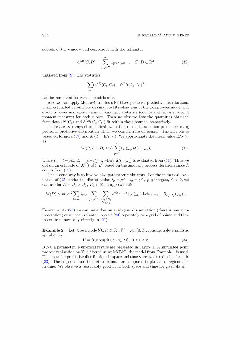
Example 2. Let A be a circle b(0, r) ⊂ R2, W = A×[0, T ], consider a deterministicspiral curve
Y = {t, t cos(βt), t sin(βt)}, 0 < t < r, (34)
β > 0 a parameter. Numerical results are presented in Figure 1. A simulated pointprocess realization on Y is filtered using MCMC, the model from Example 1 is used.The posterior predictive distributions in space and time were evaluated using formula(33). The empirical and theoretical counts are compared in planar subregions andin time. We observe a reasonably good fit in both space and time for given data.
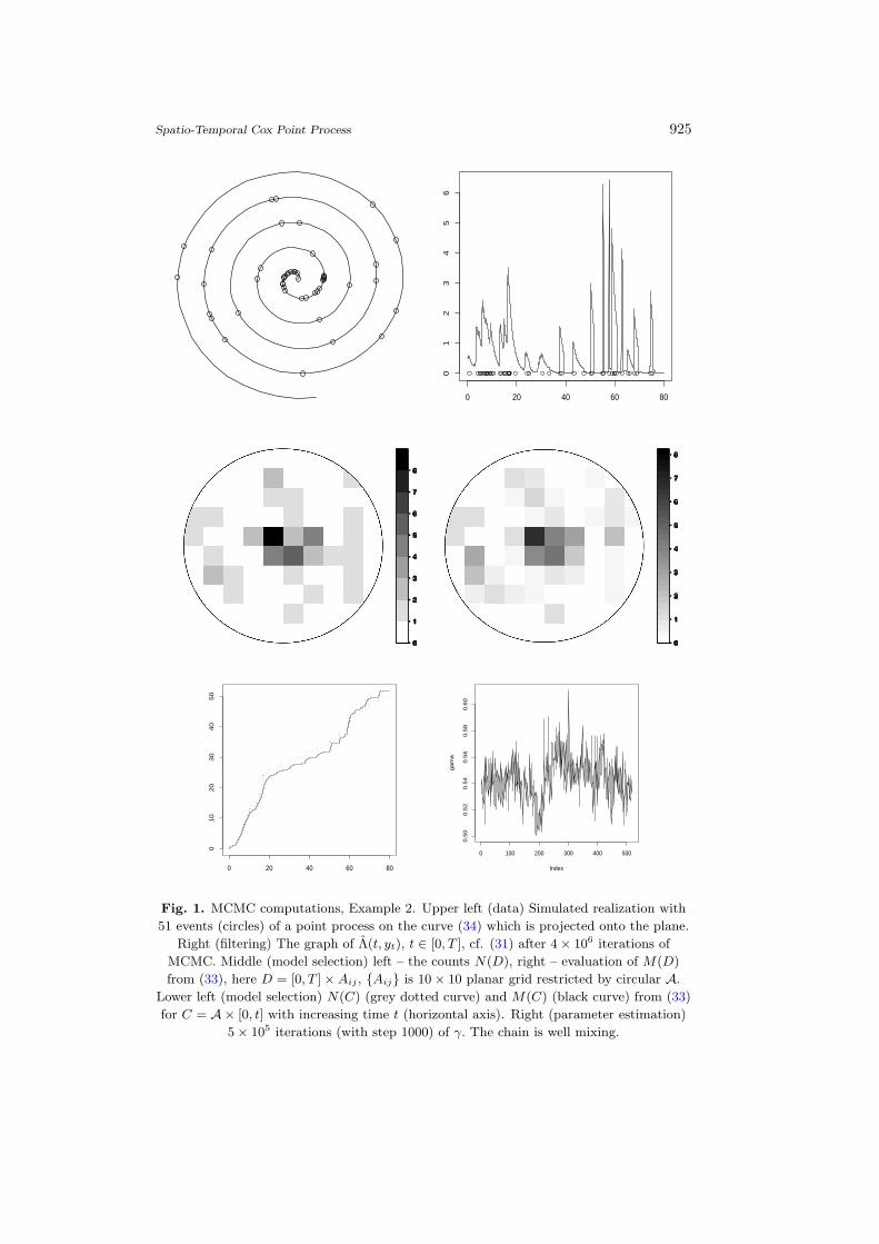
Spatio-Temporal Cox Point Process 925
0 20 40 60 80
01
23
45
6
0 20 40 60 80
010
20
30
40
50
0 100 200 300 400 500
0.5
00.5
20.5
40.5
60.5
80.6
0
Index
gam
a
Fig. 1. MCMC computations, Example 2. Upper left (data) Simulated realization with
51 events (circles) of a point process on the curve (34) which is projected onto the plane.
Right (filtering) The graph of Λ(t, yt), t ∈ [0, T ], cf. (31) after 4 × 10⁶ iterations of
MCMC. Middle (model selection) left – the counts N(D), right – evaluation of M(D)
from (33), here D = [0, T ] × Aij , {Aij} is 10 × 10 planar grid restricted by circular A.
Lower left (model selection) N(C) (grey dotted curve) and M(C) (black curve) from (33)
for C = A× [0, t] with increasing time t (horizontal axis). Right (parameter estimation)
5 × 10⁵ iterations (with step 1000) of γ. The chain is well mixing.
926 B. FRCALOVA AND V. BENES
6. RESIDUAL ANALYSIS
The model selection procedures from the previous section enable to compare variousmodels but they do not present a proper goodness-of-fit test. The Monte–Carlo testfor summary statistics, when not rejected, does not guarantee the validity of themodel on a given significance level. The residual analysis does a better job in thisdirection. For temporal and spatio-temporal point processes it is well developed, see[17], based on the conditional intensity and martingale theory in time. The purelyspatial case is more complicated and the Papangelou conditional intensity is recom-mended as the basic tool by [1]. The authors note that spatial Cox processes are hardto analyze since with the exceptions when the density w.r.t. unit Poisson processexists in a closed form, the Papangelou conditional intensity is not computationallytractable.
For a Cox point process X (either temporal, spatial or spatio-temporal) withdriving intensity measure Λm we can define an innovation process generally as
I(B) = X(B) − E[Λm(B) | X], B ∈ B. (35)
It holdsEI(B) = 0.
Given a model for Λm depending on a parameter θ ∈ Rp we obtain its estimator θand we can observe how the residual process
Rθ(B) = X(B) − Eθ[Λm(B) | X] (36)
oscillates around zero. A possibility to perform a statistical test depends on the wayhow exactly the conditioning in (35),(36) is defined. In the temporal case denotingNt, t ≥ 0 the counting process corresponding to X and Λ the density of Λm, assumingthat the conditional intensity λ∗ exists and
λ∗t = lim
4t↓0
14t
E[Nt+4t − Nt | Ns, s < t]
= lim4t↓0
14t
E[E[Nt+4t − Nt | Ns, s < t; Λp, t ≤ p < t + 4t] | Ns, s < t]
= lim4t↓0
14t
E
[∫ t+4t
t
Λ(s) ds | Ns, s < t
]= E[Λ(t) | Ns, s < t]
the innovation process Nt−∫ t
0λ∗
s ds is a martingale [12]. In the spatio-temporal casedenote Ns(C) = card{x ∈ X; x ∈ [0, s] × C}, C ∈ Bd. Analogously the conditionalintensity λ∗
λ∗(t, ξ) dt dξ = E[N(dt × dξ) | Ns(C), s < t, C ∈ Bd]
of a Cox process corresponds to
E[Λ(t, ξ) | Ns(C), s < t, C ∈ Bd] (37)

Spatio-Temporal Cox Point Process 927
and
Nt(C) −∫ t
0
∫C
λ∗(s, ξ) dsdξ
is a martingale with mean zero, C ∈ B. Scaled innovations
Vh =∫
R×Rd
H(t, ξ)[N(dt × dξ) − λ∗(t, ξ) dt dξ],
where H is a predictable process, are investigated.For the Cox process on a curve studied in this paper we have an analogous
argument. Defineλ∗
s = E[Λ(s, ys)|Nu, u < s],
Nt −∫ t
0λ∗
s ds is a martingale with mean zero. For C ∈ B, C ⊂ A and a randomprocess {H(t), t ∈ [0, T ]} the scaled innovation VC is defined as
VC =∫ T
0
1C(yt)H(t)[N(dt) − λ∗t dt].
Theorem 6.1. For a nonnegative predictable process {H(t), t ∈ [0, T ]} the scaledinnovation has variance
varVC = E
[∫ T
0
1C(yt)H2(t)λ∗t dt
].
P r o o f . Denote G(t) = 1C(yt)H(t), {G(t), t ∈ [0, T ]} is a predictable process.Since by [12], Theorem 4.6.1
E
(∫ T
0
G(t)[N(dt) − λ∗t dt]
)= 0
we have (integral limits 0, T are omitted)
varVC = E
([∫G(t)N(dt)
]2)
+E
([∫G(t)λ∗
t dt
]2)
− 2E[∫
G(t)N(dt)∫
G(t)λ∗t dt
].
Using Fubini and Theorem 1 from [25] we have
varVC = E∫
G2(t)λ∗t dt
−2E[∫
G(s)λ∗sds
∫G(t)[N(dt) − λ∗
t dt]]
928 B. FRCALOVA AND V. BENES
and the second term vanishes again by [12], Theorem 4.6.1. ¤
The choiceH(t) = 1D(t)(λ∗
t )− 1
2 , D ∈ B1
leads to the Pearson innovation
Vp =∫
D
1C(yt)[(λ∗t )
− 12 N(dt) − (λ∗
t )12 dt] (38)
withvarVp = Leb{t ∈ D; yt ∈ C}.
The residual data analysis based on a realization of the Cox process on the curve
x = {τj} = {sj , ηj}j=1,...,k, sj ∈ R, ηj ∈ R2
follows. Denote Λ(s) the MCMC estimator of λ∗s. The Pearson residual correspond-
ing to (38), time t and a measurable set C ⊂ A is then
Rθ(t, C) =∑
(sl,ηl)sl≤t, ηl∈C
Λ(sl)−12 −
∫ t
0
1C(ys)[Λ(s)]12 ds. (39)
Evaluation of the sum desires k MCMC chains conditioned up to time sj , j =1, . . . , k. A problem is the integral approximation in (39) which desires either morechains (computationally demanding) or the approximation of values of Λ(s) fromchains conditioned at times larger than the argument s.
Finally Pearson residuals can be plotted at times 0 < t1 < · · · < tn = T withbounds 2σi at ti,
σi = [Leb{t ≤ ti; yt ∈ C}] 12 .
7. CONCLUSIONS
In the paper a model of a spatio-temporal Cox point process with driving intensitybased on background driving Levy process is investigated. We derive basic propertiesof the model by means of the closed form of the generating functional. An importantcase where the events of the process lie on a curve, is studied in detail, underthe assumption that the curve is independent of the driving intensity. Then thenonlinear filtering problem is solved using the Bayesian approach. Densities withrespect to Poisson process of both the Cox process and the background drivingcompound Poisson process are involved. Markov chain Monte Carlo enables todraw approximately from the posterior distribution and make the desired inference.Posterior predictive distributions evaluate the model selection.
There have been essentially two approaches to modeling in spatio-temporal pointprocesses which have played different roles. The use of conditional intensity enablesthe residual analysis but less formulas for basic characteristics analysis. Models notbased on conditioning serve in the opposite way. In our paper within the Levy basedmodeling and stochastic simulations we tried to achieve both as is shown in the final
Spatio-Temporal Cox Point Process 929
section. Filtering and statistics can be done simultaneously, the procedures whichhave been mainly solely investigated in previous studies. The Bayesian MCMCof space-time realizations is fast enough for filtering while the residual analysis iscomputationally demanding in our setting. This procedure is more easily performedusing sequential Monte Carlo methods [18] within a conditional intensity model.
ACKNOWLEDGEMENT
The authors thank to the referees for valuable comments and suggestions. The research wassupported by grants of the Grant Agency of the Academy of Sciences of the Czech Republic(Grant 101120604), the Ministry of Education, Youth and Sport of the Czech Republic(Project MSM 0021620839) and the Czech Science Foundation (Grant 201/05/H007).
(Received April 7, 2008.)
REFERE NC ES
[1] A. Baddeley, R. Turner, J. Møller, and M. Hazelton: Residual analysis for spatialpoint processes (with discussion). J. Royal Stat. Soc. B 67 (2005), 617–666.
[2] O. Barndorff-Nielsen and N. Shephard: Non-Gaussian Ornstein–Uhlenbeck basedmodels and some of their uses in financial economics. J. Royal Stat. Soc. B 63 (2001),167–241.
[3] O. Barndorff-Nielsen and J. Schmiegel: Levy based tempo-spatial modelling; withapplications to turbulence. Usp. Mat. Nauk 159 (2004), 63–90.
[4] V. Benes and B. Frcalova: Modelling and simulation of a neurophysiological experi-ment by spatio-temporal point processes. Image Anal. Stereol. 1 (2008), 27, 47–52.
[5] P. Bremaud: Point Process and Queues. Springer, New York 1981.
[6] A. Brix and J. Møller: Space-time multi type log Gaussian Cox processes with a viewto modelling weed data. Scand. J. Statist. 28 (2002), 471–488.
[7] A. Brix and P. Diggle: Spatio-temporal prediction for log-Gaussian Cox processes. J.Royal Statist. Soc. B 63 (2001), 823–841.
[8] M.A. Clyde and R. L. Wolpert: Nonparametric function estimation using overcom-plete dictionaries. Bayesian Statistics 8 (2007), 1–24.
[9] R. Cont and P. Tankov: Financial Modelling with Jump Processes. Chapman andHall/CRC, Boca Raton 2004.
[10] D. Daley and D. Vere-Jones: An Introduction to the Theory of Point Processes I, II.Springer, New York 2003, 2008.
[11] A. Ergun, R. Barbieri, U.T. Eden, M. A. Wilson, and E. N. Brown: Construction ofpoint process adaptive filter algorithms for neural systems using sequential MonteCarlo methods. IEEE Trans. Biomed. Engrg. 54 (2007), 3, 307–326.
[12] P.M. Fishman and D. Snyder: The statistical analysis of space-time point processes.IEEE Trans. Inform. Theory 22 (1976), 257–274.
[13] G. Hellmund, M. Prokesova, and E. Vedel Jensen: Levy based Cox point processes.Adv. Appl. Probab. 40 (2008), 3, 603–629.
[14] M. Jacobsen: Point Processes Theory and Applications. Marked Point and PiecewiseDeterministic Processes. Birkhauser, Boston 2006.
930 B. FRCALOVA AND V. BENES
[15] A. F. Karr: Point Processes and Their Statistical Inference. Marcel Dekker, New York1985.
[16] P. Lansky and J. Vaillant: Stochastic model of the overdispersion in the place celldischarge. BioSystems 58 (2000), 27–32.
[17] R. Lechnerova, K. Helisova, and V. Benes: Cox point processes driven by Ornstein–Uhlenbeck type processes. Method. Comp. Appl. Probab. 10 (2008), 3, 315–336.
[18] J. Møller and R. Waagepetersen: Statistics and Simulations of Spatial Point Pro-cesses. World Sci., Singapore 2003.
[19] J. Møller and C. Diaz-Avalos: Structured spatio-temporal shot-noise Cox point pro-cess models, with a view to modelling forest fires. Scand. J. Statist. (2009), to appear.
[20] Y. Ogata: Space-time point process models for eartquake occurences. Ann. Inst.Statist. Math. 50 (1998), 379–402.
[21] J. Pedersen: The Levy–Ito Decomposition of Independently Scattered Random Mea-sure. Res. Report 2, MaPhySto, University of Aarhus 2003.
[22] R.D. Peng, F. P. Schoenberg, and J. Woods: A space-time conditional intensity modelfor evaluating a wildfire hazard risk. J. Amer. Statist. Assoc. 100 (2005), 469, 26–35.
[23] B. S. Rajput and J. Rosinski: Spectral representations of infinitely divisible processes.Probab. Theory Related Fields 82 (1989), 451–487.
[24] G. Roberts, O. Papaspiliopoulos, and P. Dellaportas: Bayesian inference for non-Gaussian Ornstein–Uhlenbeck stochastic volatility processes. J. Royal Statist. Soc. B66 (2004), 369–393.
[25] D. L. Snyder: Filtering and detection for doubly stochastic Poisson processes. IEEETrans. Inform. Theory 18 (1972), 91–102.
[26] F. P. Schoenberg, D.R. Brillinger, and P. M. Guttorp: Point processes, spatial-temporal. In: Encycl. of Environmetrics (A. El. Shaarawi and W. Piegorsch, eds.),Vol. 3, Wiley, New York 2003, pp. 1573–1577.
[27] J. Zhuang: Second-order residual analysis of spatiotemporal point processes andapplications in model evaluation. J. Royal Statist. Soc. B 68 (2006), 635–653.
Blazena Frcalova and Viktor Benes, Department of Probability and Mathematical
Statistics, Faculty of Mathematics and Physics – Charles University in Prague,
Sokolovska 83, 186 75 Praha 8. Czech Republic.
e-mails: [email protected], [email protected]