Temporal Modelling of Mobile Data Traffic Applications

Temporal Modelling of Mobile Data Traffic Applications

for Network Optimisation

Ana Margarida Pina Simões

Thesis to obtain the Master of Science Degree in

Electrical and Computer Engineering

Supervisor: Prof. Luís Manuel de Jesus Sousa Correia

Examination Committee

Chairperson: Prof. José Eduardo Charters Ribeiro da Cunha Sanguino

Supervisor: Prof. Luís Manuel de Jesus Sousa Correia

Member of Committee: Prof. Paulo Luís Serras Lobato Correia

Eng. Paulino Anibal Pereira Serra de Magalhães Corrêa

May 2017

iii

To my beloved family

v

Acknowledgements

I would like to thank and express my sincere gratitude to Prof. Luís M. Correia for the opportunity to

develop my master thesis under his supervision and guidance, and for allowing me to do work in a

current and leading topic, in collaboration with a major telecommunications operator in Portugal. I am

very thankful for the weekly meetings and all the advice, knowledge, time and encouragement , given to

me. The discipline and work ethics bestowed on me will be remembered, and will follow me into my

professional life.

To Eng. Paulino Corrêa, Eng. João Fernandes and Eng. Alexandre Rodrigues, from Vodafone, for the

time and effort dispended in meetings and feedback, and the availability to provide me with data from a

live network.

I would like to thank for the valuable experience of being a part of the Group for Research On Wireless

(GROW) and all the support and friendship I received from my colleagues.

To my mother, Fatima Pina, and my father, Carlos Simões, I want to thank for always pushing me to do

better, and is an honour to follow in your footsteps. To my family and parents, I am grateful for your love

and kindness. A special mention to my dog, whom I miss.

vii

Abstract

The increasing usage and diversity of data applications, in cellular mobile networks, is changing traffic

consumption patterns. Studying and gaining a broader understanding of how impactful people’s daily

lives are in application utilisation, device preferences, operating systems’ share, and network resource

demands, in the time domain, for both weekdays and weekends, is key to increasing efficient resource

usage, network optimisation, and reducing the operators’ costs. The purpose of this work is to

statistically characterise the observed data by providing visual aids and mathematical models, thus

highlighting patterns and better realising the implicit behaviours associated to a live c ellular network.

This document includes a background on UMTS, LTE, services and applications. A review of the state

of the art on the matters of the study is featured. The entities in analysis are the number of active users

and traffic usage, for both download and upload. A statistical modelling methodology is used to fit traffic

usage, and 8 regression models are obtained, for each study case, and then compared and ranked

based on goodness of fit statistics’ results, so that the models that best approximated the data are

selected. The regression results suggest that a model resembling a tree stump, with 3 sections, is an

adequate representation of the average traffic usage, for both download and upload, considering

weekdays and weekends, for the streaming application, the smartphone device, and the Android and

iOS operating systems.

Keywords

UMTS; LTE; Mobile Services; Data Applications; Mobile Network Design and Optimisation; Statistical

Modelling; Temporal Traffic Models.

viii

Resumo

O consumo de tráfego na rede móvel tem demonstrado alterações dos padrões de utilização dos

serviços e aplicações de dados. Os utilizadores geram diferentes tipos de tráfego, dependendo das

suas preferências, da altura do dia e da semana. O desenvolvimento de modelos, com recurso a

informação proveniente da rede móvel, vai permitir caracterizar a utilização de tráfego, as preferências

de terminal e de sistema operativo, no domínio do tempo, tanto para os dias de semana como de fim

de semana; o que pode contribuir para a eficiência da utilização de recursos, otimização da rede móvel,

e redução de custos para o operador. O propósito deste trabalho é caracterizar estatisticamente os

dados observados, fornecendo ferramentas visuais e modelos analíticos. Este documento aborda as

redes de UMTS e LTE, serviços e aplicações; e inclui o estado da arte que motiva o trabalho. As

entidades em análise são o número de utilizadores e o tráfego, em download e upload. Uma

metodologia de modelação estatística é usada para ajustar 8 modelos de tráfego aos dados,

compará-los e ordená-los, de acordo com os resultados das estatísticas para a qualidade do

ajustamento, por forma a selecionar os modelos que melhor explicam os dados. O resultado do ajuste

de curvas, sugere que um modelo que se assemelha a um tronco de árvore, representa

adequadamente a utilização média de tráfego, para streaming, smartphone, Android, e iOS, tanto para

download como upload, considerando tanto os dias de semana, como de fim de semana.

Palavras-chave

UMTS; LTE; Serviços Móveis; Aplicações de Dados; Otimização e Dimensionamento de Redes Móveis ;

Modelação Estatística; Modelos de Tráfego no Tempo.

ix

Table of Contents

Acknowledgements ................................................................................................................. v

Abstract ................................................................................................................................. vii

Resumo ................................................................................................................................ viii

Table of Contents ................................................................................................................... ix

List of Figures ........................................................................................................................ xi

List of Tables.........................................................................................................................xiii

List of Acronyms .................................................................................................................... xvi

List of Symbols ...................................................................................................................... xx

List of Software ................................................................................................................... xxiii

1 Introduction 1

1.1 Overview and Motivation ................................................................................................ 2

1.2 Problem Definition and Content....................................................................................... 5

2 Fundamental Concepts 7

2.1 UMTS ........................................................................................................................... 8

2.2 LTE ............................................................................................................................... 9

2.3 Services and Applications ............................................................................................. 11

2.4 Traffic Models .............................................................................................................. 14

2.5 State of the Art ............................................................................................................. 17

3 Model Development and Implementation 25

3.1 Data Collection ............................................................................................................ 26

3.1.1 Training Data Set ............................................................................................. 26

3.1.2 Development Overview .................................................................................... 28

3.1.3 Descriptive Statistical Analysis.......................................................................... 29

3.1.4 Goodness of Fit Tests ...................................................................................... 30

3.1.5 Goodness of Fit Statistics ................................................................................. 31

3.2 Development Conditions and Considerations ................................................................. 32

3.2.1 Data Collection Analysis................................................................................... 32

3.2.2 Data Statistical Distribution Assessment ............................................................ 34

3.3 Exploratory Data Analysis............................................................................................. 36

3.3.1 Data Ratios ..................................................................................................... 36

3.3.2 Global Results ................................................................................................. 38

3.3.3 Applications Results......................................................................................... 40

3.3.4 Devices Results ............................................................................................... 41

3.3.5 Operating Systems Results .............................................................................. 43

3.3.6 Maximum Traffic Percent Change ..................................................................... 45

x

3.4 Model Catalogue.......................................................................................................... 47

3.5 Implementation Methodology ........................................................................................ 49

3.5.1 Data Structuring and Processing....................................................................... 49

3.5.2 Fitting Process................................................................................................. 50

3.6 Model Comparison and Ranking ................................................................................... 55

3.6.1 Goodness of Fit Statistics Results ..................................................................... 55

3.6.2 Best Ranked Models ........................................................................................ 60

3.6.3 General Models ............................................................................................... 62

3.7 Regression Results ...................................................................................................... 64

4 Results Analysis 73

4.1 Models’ Assessment and Applicability ........................................................................... 74

4.1.1 Validation Data Set .......................................................................................... 74

4.1.2 Global Traffic Model ......................................................................................... 78

4.2 Model Collections......................................................................................................... 82

4.2.1 Applications Models ......................................................................................... 82

4.2.2 Devices Models ............................................................................................... 84

4.2.3 Operating Systems Models............................................................................... 86

4.2.4 Considerations and Recommendations ............................................................. 87

5 Conclusions 89

A. Regression Models with Training Data 95

References 107

xi

List of Figures Figure 1.1 – Mobile subscriptions outlook (adapted from [2]). ............................................................ 3

Figure 1.2 – Mobile traffic outlook (adapted from [2]). ....................................................................... 3

Figure 1.3 – Mobile traffic by application category (adapted from [2]). ................................................ 4

Figure 1.4 – Connected devices (billions) (adapted from [5]). ............................................................ 4

Figure 2.1 – UMTS network architecture (adapted from [7]). ............................................................. 8

Figure 2.2 – System architecture for an E-UTRAN only network (extracted from [12]). ...................... 10

Figure 2.3 – Voice and data traffic models extracted from the literature. ........................................... 17

Figure 2.4 – Distribution map of BSs, depicting different regions (extracted from [29]). ..................... 17

Figure 2.5 – Diurnal application usage profile (extracted from [25]). ................................................. 20

Figure 2.6 – Usage profiles for each device type (extracted from [34]). ............................................ 20

Figure 2.7 – Usage of the Google Wi-Fi network, for a month (extracted from [23]). .......................... 21

Figure 2.8 – Daily traffic consumption in Europe (extracted from [35]). ............................................. 22

Figure 2.9 – Daily traffic profiles (extracted from [24]). .................................................................... 22

Figure 2.10 – Diurnal patterns for different genres of smartphone applications (extracted from [36]). . 23

Figure 2.11 – Traffic in minutes during weekday and weekends (extracted from [37]). ...................... 23

Figure 3.1 – Framework................................................................................................................ 28

Figure 3.2 – Development overview. ............................................................................................. 28

Figure 3.3 – Traffic usage data observations over 39 days, from 2016/03/12 to 2016/04/19. ............. 33

Figure 3.4 – APP_GROUP Streaming. .......................................................................................... 33

Figure 3.5 – APP_GROUP Streaming Histogram. .......................................................................... 34

Figure 3.6 – Weekdays Hour Weights............................................................................................ 38

Figure 3.7 – Weekdays Traffic Ratios. ........................................................................................... 39

Figure 3.8 – Weekdays APP_GROUP Hourly Ratios. ..................................................................... 40

Figure 3.9 – Weekdays APP_GROUP Daily Ratios. ....................................................................... 40

Figure 3.10 – Weekdays APP_GROUP Aggregated Daily Ratios. ................................................... 41

Figure 3.11 – Weekdays DEV_TYPE Hourly Ratios........................................................................ 42

Figure 3.12 – Weekdays DEV_TYPE Daily Ratios. ......................................................................... 42

Figure 3.13 – Weekdays DEV_TYPE Aggregated Daily Ratios........................................................ 43

Figure 3.14 – Weekdays OP_SYS Hourly Ratios............................................................................ 44

Figure 3.15 – Weekdays OP_SYS Daily Ratios. ............................................................................. 44

Figure 3.16 – Weekdays OP_SYS Aggregated Daily Ratios............................................................ 44

xii

Figure 3.17 – Model Fitting Options. .............................................................................................. 48

Figure 3.18 – Goodness of fit statistics. ......................................................................................... 52

Figure 3.19 – Data Processing. ..................................................................................................... 53

Figure 3.20 – Fitting Process. ....................................................................................................... 54

Figure 3.21 – Profile definition. ...................................................................................................... 55

Figure 3.22 – Structure data. ........................................................................................................ 55

Figure 3.23 – Goodness of fit statistics’ colour criteria..................................................................... 56

Figure 3.24 – APP_GROUP Streaming General Model. .................................................................. 66

Figure 3.25 – APP_GROUP Streaming General Model 00:00 – 24:00. ............................................ 66

Figure 3.26 – DEV_TYPE Smartphone General Model. .................................................................. 69

Figure 3.27 – DEV_TYPE Smartphone General Model 00:00 – 24:00. ............................................. 70

Figure 3.28 – OP_SYS Android General Model. ............................................................................. 71

Figure 3.29 – OP_SYS Android General Model 00:00 – 24:00. ....................................................... 71

Figure 4.1 – APP_GROUP and DEV_TYPE Prediction Assessment. ............................................... 79

Figure 4.2 – App Collection Prediction Global Traffic for the General Models. .................................. 81

Figure 4.3 – Dev Collection Prediction Global Traffic for the General Models. .................................. 82

Figure 4.4 – App Collection General Models. ................................................................................. 83

Figure 4.5 – Dev Collection General Models. ................................................................................. 85

Figure 4.6 – OpS Collection Android and iOS General Models. ....................................................... 87

xiii

List of Tables Table 2.1 – Data rates in UMTS (extracted from [9]). ........................................................................ 9

Table 2.2 – Relationship between the bandwidth, the number of sub-carries and the number of

resource blocks (extracted from [9]). ...................................................................... 11

Table 2.3 – UE’s categories in LTE (adapted from [14]) .................................................................. 11

Table 2.4 – UMTS QoS Classes (adapted from [9]). ....................................................................... 12

Table 2.5 – Standardised QCIs for LTE (extracted from [16]). ......................................................... 13

Table 2.6 – Services characteristics (adapted from [17]). ................................................................ 13

Table 2.7 – Mainstream mobile internet categories characteristics (adapted from [18]). .................... 14

Table 2.8 – Data applications characterisation. .............................................................................. 14

Table 2.9 – Geotypes characterisation (adapted from [20]). ............................................................ 15

Table 2.10 – Area, population and mobile traffic by geotype in Portugal (adapted from [20]). ............ 15

Table 2.11 – Theoretical cell radius (km) (adapted from [20]). ......................................................... 15

Table 2.12 – Application level traffic growth forecast (adapted from [15]). ........................................ 19

Table 3.1 – Length of day for March and April, for the Lisbon area. ................................................. 26

Table 3.2 – Training set description. .............................................................................................. 27

Table 3.3 – Percentages of non-rejected decisions, for APP_GROUP, in the assessment at 5% level

of significance, to the normal distribution, using the Lilliefors test. ............................ 35

Table 3.4 – Percentages of non-rejected decisions, for DEV_TYPE, in the assessment at 5% level of

significance, to the normal distribution, using the Lilliefors test................................. 35

Table 3.5 – Percentages of non-rejected decisions, for OP_SYS, in the assessment at 5% level of

significance, to the normal distribution, using the Lilliefors test................................. 36

Table 3.6 – APP_GROUP Traffic Percent Change. ........................................................................ 46

Table 3.7 – DEV_TYPE Traffic Percent Change. ............................................................................ 46

Table 3.8 – OP_SYS Traffic Percent Change. ................................................................................ 47

Table 3.9 – Weekdays Download APP_GROUP. ........................................................................... 57

Table 3.10 – Weekdays Download APP_GROUP Best Models. ...................................................... 60

Table 3.11 – Weekdays Download DEV_TYPE Best Models........................................................... 61

Table 3.12 – Weekdays Download OP_SYS Best Models: Ranking................................................. 62

Table 3.13 – Weekdays Download APP_GROUP General Model. ................................................... 63

Table 3.14 – Weekdays Download DEV_TYPE General Model. ...................................................... 63

Table 3.15 – Weekdays Download OP_SYS General Model. .......................................................... 64

Table 3.16 – Weekdays Download APP_GROUP E-Mail General Model. ........................................ 67

xiv

Table 3.17 – Weekdays Download APP_GROUP FiTr General Model. ............................................ 67

Table 3.18 – Weekdays Download APP_GROUP Games General Model. ....................................... 67

Table 3.19 – Weekdays Download APP_GROUP InMe General Model. .......................................... 68

Table 3.20 – Weekdays Download APP_GROUP M2M General Model. .......................................... 68

Table 3.21 – Weekdays Download APP_GROUP Other General Model. ......................................... 68

Table 3.22 – Weekdays Download APP_GROUP P2P General Model. ........................................... 68

Table 3.23 – Weekdays Download APP_GROUP Streaming General Model.................................... 68

Table 3.24 – Weekdays Download APP_GROUP VoIP General Model............................................ 69

Table 3.25 – Weekdays Download APP_GROUP WebAp General Model. ....................................... 69

Table 3.26 – Weekdays Download DEV_TYPE Smartphone General Model. ................................... 70

Table 3.27 – Weekdays Download OP_SYS Android General Model. .............................................. 72

Table 4.1 – Length of day for September and October, for the Lisbon area. ..................................... 74

Table 4.2 – Weekdays Download APP_GROUP. ........................................................................... 75

Table 4.3 – APP_GROUP Prediction Assessment.......................................................................... 80

Table 4.4 – DEV_TYPE Prediction Assessment. ............................................................................ 80

Table A.1 – APP_GROUP Best Models: Ranking. .......................................................................... 96

Table A.2 – APP_GROUP General Model. .................................................................................... 96

Table A.3 – Weekdays Download APP_GROUP E-Mail General Model. .......................................... 96

Table A.4 – Weekdays Download APP_GROUP FiTr Best/General Model. ...................................... 97

Table A.5 – Weekdays Download APP_GROUP Games General Model. ........................................ 97

Table A.6 – Weekdays Download APP_GROUP InMe Best/General Model. .................................... 98

Table A.7 – Weekdays Download APP_GROUP M2M Best/General Model. .................................... 98

Table A.8 – Weekdays Download APP_GROUP Other Best/General Model. ................................... 99

Table A.9 – Weekdays Download APP_GROUP P2P Best/General Model. ..................................... 99

Table A.10 – Weekdays Download APP_GROUP Streaming General Model. ................................ 100

Table A.11 – Weekdays Download APP_GROUP VoIP General Model. ........................................ 100

Table A.12 – Weekdays Download APP_GROUP WebAp Best/General Model. ............................. 101

Table A.13 – DEV_TYPE Best Models: Ranking. ......................................................................... 101

Table A.14 – DEV_TYPE General Model. .................................................................................... 101

Table A.15 – Weekdays Download DEV_TYPE Hotspots General Model. ...................................... 102

Table A.16 – Weekdays Download DEV_TYPE Others Best/General Model. ................................. 102

Table A.17 – Weekdays Download DEV_TYPE Pens General Model. ........................................... 103

Table A.18 – Weekdays Download DEV_TYPE Routers Best/General Model. ............................... 103

Table A.19 – Weekdays Download DEV_TYPE Smartphone Best/General Model. ......................... 104

Table A.20 – Weekdays Download DEV_TYPE Tablet Best/General Model. .................................. 104

xv

Table A.21 – OP_SYS Best Models: Ranking. ............................................................................. 104

Table A.22 – OP_SYS General Model. ........................................................................................ 105

Table A.23 – Weekdays Download OP_SYS Android General Model. ........................................... 105

Table A.24 – Weekdays Download OP_SYS Others General Model. ............................................. 105

Table A.25 – Weekdays Download OP_SYS Windows Best/General Model. .................................. 106

Table A.26 – Weekdays Download OP_SYS iOS Best/General Model. .......................................... 106

xvi

List of Acronyms 1G 1st Generation

2G 2nd Generation

3G 3rd Generation

3GPP 3rd Generation Partnership Project

4G 4th Generation

5G 5th Generation

ACD Adjusted Coefficient of Determination

ANACOM Autoridade Nacional de Comunicações

App Applications

BS Base Station

CA Carrier Aggregation

CAGR Compound Annual Growth Rate

CD Coefficient of Determination

CDF Cumulative Distribution Function

CI Confidence Interval

CN Core Network

CP Control Plane

CS Circuit Switch

D2D Device-to-Device

DCT Discrete Cosine Transform

DDGM Data Double Gaussian Model

Dev Devices

DGM Double-Gaussian Model

DL Download Link

DS-CDMA Direct-Sequence Code Division Multiple Access

DTrM Data Trapezoidal Model

EDGE Enhanced Data rates for GSM Evolution

EPC Evolved Packet Core

EPS Evolved Packet System

E-UTRAN Evolved UTRAN

FDD Frequency Division Duplex

FiTr File Transfer Applications

FTP File Transfer Protocol

GGSN Gateway General Packet Radio System Support Node

GMSC Gateway Mobile Services Switching Centre

GOF Goodness Of Fit

xvii

GPRS General Packet Radio System

GSM Global System for Mobile Communications

HLR Home Location Register

HSDPA High Speed Downlink Packet Access

HSPA High Speed Packet Access

HSS Home Subscription Service

HSUPA High Speed Uplink Packet Access

HTTP Hypertext Transfer Protocol

IM Instant Messaging

IMS IP Multimedia Sub-System

InMe Instant Messaging Applications

IoT Internet of Things

IP Internet Protocol

KPI Key Performance Indicator

LCR Low Chip Rate

LTE Long Term Evolution

LTE-A Long Term Evolution - Advanced

M2M Machine-to-Machine

MBMS Multimedia Broadcast Multicast Services

MBR Maximum Bit Rate

ME Mobile Equipment

MGBR Minimum Guaranteed Bit Rate

MIMO Multiple Input and Multiple Output

MM Mobility Management

MME Mobility Management Entity

MMS Multimedia Messaging Service

MNO Mobile Network Operator

MSC Mobile Services Switching Centre

MSE Mean Squared Error

MSISDN Mobile Subscriber Integrated Service Digital Network Number

MT Mobile Terminal

NU Number of Active Users

OFDMA Orthogonal Frequency Division Multiple Access

OpS Operating Systems

P2P Peer-to-Peer

PC Personal Computer

PCC Policy and Charging Control

PCRF Policy and Charging Rules Function

PDA Personal Digital Assistant

PDF Probability Density Function

xviii

PDN Packet Data Network

P-GW Packet Data Network Gateway

PLMN Public Land Mobile Network

PS Packet Switch

PyM Pyramid Model

QAM Quadrature Amplitude Modulation

QCI QoS Class Identifier

QoS Quality of Service

QPSK Quadrature Phase Shift Keying

RAN Radio Access Network

RMSE Root Mean Squared Error

RNC Radio Network Controller

RNS Radio Network Subsystem

RRM Radio Resource Management

SAE System Architecture Evolution

SC-FDMA Single Carrier Frequency Division Multiple Access

SGSN Serving General Packet Radio System Support Node

S-GW Serving Gateway

SIM Subscriber Identity Module

SIP Session Initiation Protocol

SMS Short Messaging Service

SNS Social Networking Services

SPPP Spatial Poisson Point Process

SwM Swing Model

TCP Transmission Control Protocol

TDD Time Division Duplex

TE Terminal Equipment

TrM Trapezoidal Function Model

TSM Tree Stump Model

UE User Equipment

UL Upload Link

UMTS Universal Mobile Telecommunications System

UP User Plane

USIM Universal Subscriber Identity Module

UTRAN UMTS Terrestrial Radio Access Network

VLR Visitor Location Register

VoIP Voice over Internet Protocol

WAP Wireless Access Protocol

WCDMA Wideband Code Division Multiple Access

WD Weekdays

xix

WE Weekends

WebAp Web Applications

Wi-Fi Wireless Fidelity

xx

List of Symbols

α level of significance

Δ𝑅𝑛 percent change

√ε2̅ root mean squared error

μ̅ global average

μ𝐾 average

μ𝑖 average of the 𝑖𝑡ℎ observation

σ̅ average standard deviation

σ𝑖 standard deviation of the 𝑖𝑡ℎ observation

σ𝐾 dispersion factor

τ1 first gaussian deviation

τ2 second gaussian deviation

𝑎𝑚𝑑𝑙 auxiliary model coefficient 2

𝑎𝑔𝑎𝑢𝑠𝑠 double gaussian model

𝑎𝑡𝑟𝑑1 first exponential initial value

𝑎𝑡𝑟𝑑2 second exponential initial value

𝑏𝑚𝑑𝑙 auxiliary model coefficient 1

𝑏𝑡𝑟𝑑1 first exponential decay factor

𝑏𝑡𝑟𝑑2 second exponential decay factor

𝑏𝐾 initial value

𝑐 collection

𝑐𝐾 vertical offset

𝑐𝑡𝑟𝑑 linear constant value

𝑐𝑡𝑟𝑑2 second exponential offset

𝑑 day

𝐷𝐿𝑖𝑙𝑙𝑖𝑒𝑓𝑜𝑟𝑠 Lilliefors’ test statistic

𝐸 entity

ℎ hour

𝑓 auxiliary model

𝑓𝑒𝑥𝑝 𝐾 exponential equation

𝑓𝑔𝑎𝑢𝑠𝑠 𝐾 gaussian equation

𝑓𝑙𝑖𝑛 𝐾 linear equation

𝑓𝑛 traffic model for the 𝑛𝑡ℎ case

𝑓𝑡𝑟𝑎𝑝𝑑𝑎𝑡𝑎 data trapezoidal model

𝑓𝐷𝑂𝑈𝐵𝐿𝐸 𝐺𝐴𝑈𝑆𝑆𝐼𝐴𝑁 double gaussian model

𝑓𝑇𝑅𝐼𝑃𝐿𝐸 𝐺𝐴𝑈𝑆𝑆𝐼𝐴𝑁 triple gaussian model

𝑓𝐺𝐴𝑈𝑆𝑆𝐼𝐴𝑁 gaussian model

xxi

𝑓𝑃𝑌𝑅𝐴𝑀𝐼𝐷 pyramid model

𝑓𝑇𝐻𝑂𝑅𝑁𝐿 thorn left model

𝑓𝑇𝐻𝑂𝑅𝑁𝑅 thorn right model

𝑓𝑇𝑅𝐴𝑃𝑍𝑂𝐼𝐷 trapezoid model

𝑓𝑇𝑅𝐸𝐸 𝑆𝑇𝑈𝑀𝑃 tree stump model

𝐹 auxiliary function

𝐹𝑋 theoretical CDF

𝐹𝑋 empirical CDF

𝑘𝐾 decay rate

𝑙 link

𝑚𝐾 scope

𝑛 case

𝑁 number of observations

𝑁𝐷 number of days

𝑁𝐻 number of hours

𝑁𝑛 number of cases

𝑁𝑆 number of samples

𝑁𝑢 number of active users

𝑝 profile

𝑝1 first gaussian amplitude

𝑝2 second gaussian amplitude

𝑃 number of predictors

𝑅2 coefficient of determination value

𝑅𝑎𝑑𝑗2 adjusted coefficient of determination value

𝑅𝑛 input ratios

𝑅𝑜𝑏𝑠 observed input

𝑅𝑟𝑒𝑓 reference input

𝑅𝑤 weighted average

𝑡 shifted hour time

𝑡1 morning shifted peak hour

𝑡2 afternoon shifted peak hour

𝑡𝐾 translation in time

𝑡𝑙 shifted lunch hour

𝑡𝑡𝑟𝑑1𝑠ℎ𝑖𝑓𝑡 first breakpoint shifted hour value

𝑡𝑡𝑟𝑑2𝑠ℎ𝑖𝑓𝑡 second breakpoint shifted hour value

𝑇 traffic usage

𝑇𝐺 global traffic model

𝑇𝑛 maximum traffic for the 𝑛𝑡ℎ case

𝑢𝐾 scaling factor

𝑣𝐾 vertical offset

𝑤𝑛 weight

xxii

𝑤ℎ𝐸̅̅ ̅̅ average hour weight, for the ℎ hour, and 𝐸 entity

𝑤𝐻 ℎ,𝑛𝐸̅̅ ̅̅ ̅̅ ̅̅ average hourly ratio, for the ℎ hour, 𝑛 case, and 𝐸 entity

𝑤𝐷 ℎ,𝑛𝐸̅̅ ̅̅ ̅̅ ̅̅ average daily ratio, for the ℎ hour, 𝑛 case, and 𝐸 entity

𝑤𝑛𝐸̅̅ ̅̅ average aggregated daily ratio, for the 𝑛 case, and 𝐸 entity

𝑦 average of the observed values

𝑦𝑐𝑜𝑛𝑠𝑡 normalisation constant

𝑦𝑖 𝑖𝑡ℎ observed value (data set)

𝑦𝑖 𝑖𝑡ℎ predicted value (model)

𝑦𝑗 𝑗 𝑡ℎ sample

𝑦𝑗𝑁𝑜𝑟𝑚 normalised observed values

xxiii

List of Software MATLAB R2016a Numerical simulation software

Microsoft Excel 2016 Spreadsheet software

Microsoft Visio 2016 Diagramming and vector graphics software

Microsoft Word 2016 Word processor software

1

Chapter 1

Introduction

1 Introduction

The present chapter establishes the framework of the thesis and presents an overview on the current

mobile communications scenario. The motivations are addressed, the problem definition is presented,

and the structure for the thesis is provided.

2

1.1 Overview and Motivation

The continuous work and advances in mobile communications, which translates into the development

of new technologies, provide continuity to the evolving systems, and allow existing equipment to stay at

use; these efforts are grouped into generations. The aim of each new generation is to release features

and functionalities that can deliver higher data rates and Quality of Service (QoS), with increased cost

efficiency [1]. Introduced in the 1980s, the 1st Generation (1G) of mobile communications only provided

voice, with some supplementary services, and consisted of independent analogue systems. The

analogue systems had limitations which restricted the general use of mobile devices. The introduction

of digital systems allowed an increase in QoS, and the possibility to develop more compact devices.

The Global System for Mobile Communications (GSM), introduced in the 1990s, was the first digital

mobile communication system, and is known as the 2nd Generation (2G) of mobile communications. The

services introduced with 2G, included the Short Message Service (SMS), e-mail and other service

applications, at very low data rates. Originally, the system only supported circuit switching, and was

improved over time to include data communications through packet transmission, with the development

of the General Packet Radio System (GPRS), latter complemented with the radio interface

improvements in Enhanced Data rates for GSM Evolution (EDGE). The success of packet transmission

services propelled the search and development of solutions for the provision of better QoS and improved

capacity. The 3rd Generation Partnership Project (3GPP) was created to unify and standardise the

mobile communications systems’ development, while assuring compatibility with the previous systems.

The 3rd Generation (3G) of mobile communications, Universal Mobile Telecommunications System

(UMTS), was introduced in the beginning of the new millennium, with significant improvement of the

radio interface. Long Term Evolution (LTE), the 4th Generation (4G) of mobile communications, was

designed to provide improved data rates, reduced latency, reduced cost -per-bit, simplified architecture

with an all Internet Protocol (IP) network, and improved spectrum efficiency; while allowing compatibility

with previous systems. LTE-Advanced (LTE-A), introduced Carrier Aggregation (CA), enabling multiple

LTE carriers to be used together to provide higher data rates; relaying, for enhancing both coverage

and capacity; and, compatibility for heterogeneous networks. Since the development of EDGE, peak

data rates have increased more than 600 times. The 5th Generation (5G) of mobile communications is

currently under development, and aims at providing higher capacity, allowing a higher density of mobile

broadband users, supporting Device-to-Device (D2D) communications, and the increasing number of

Machine-to-Machine (M2M) communications. For better implementation of the Internet of Things (IoT),

5G is being designed to provide lower latency and lower battery consumption, than previous generations

[1].

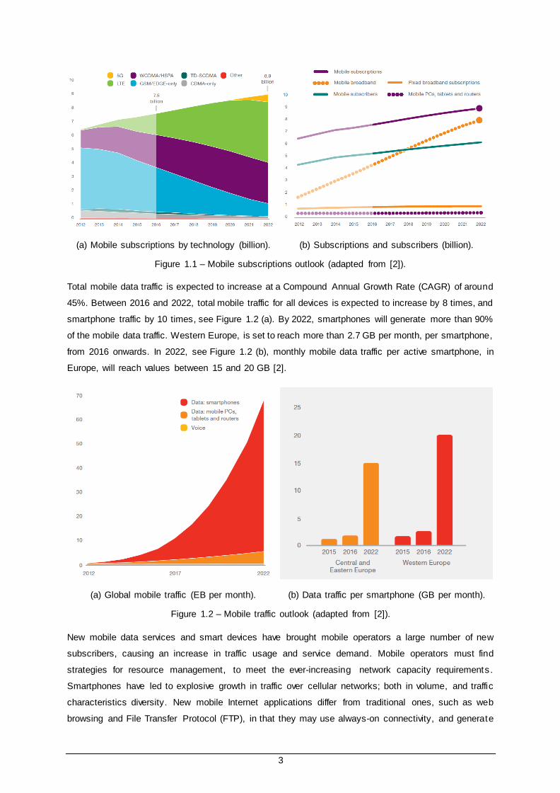
Figure 1.1 (a) depicts the number of mobile subscriptions by mobile communication technology. LTE is

anticipated to become the dominant mobile access technology in 2019. 5G networks are expected to

be available, and introduced by most operators, by 2020; and, by the end of 2022, the number of 5G

subscribers is expected to reach around 550 million. As seen in Figure 1.1 (b), from 2016 to 2022, an

increase of 1.5 billion new mobile subscribers is anticipated; and, by 2022, mobile broadband

subscriptions are expected to account for 90% of all mobile subscriptions [2].

3

(a) Mobile subscriptions by technology (billion). (b) Subscriptions and subscribers (billion).

Figure 1.1 – Mobile subscriptions outlook (adapted from [2]).

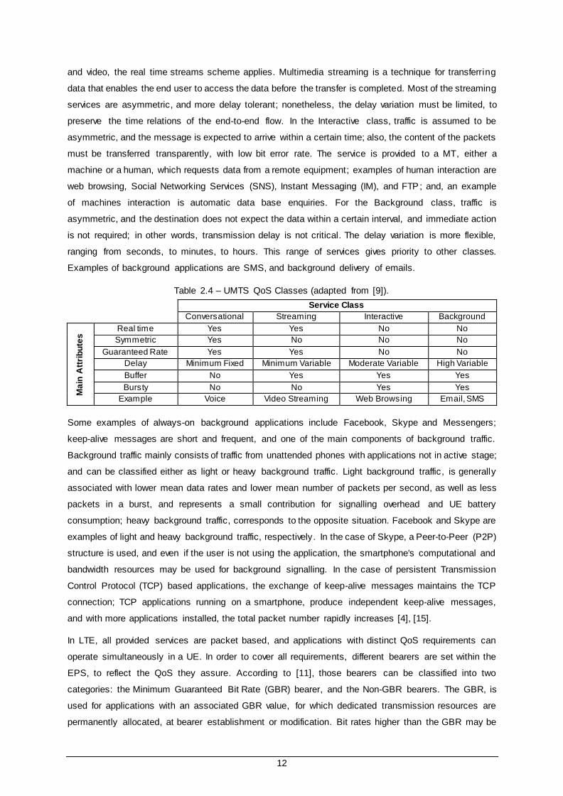
Total mobile data traffic is expected to increase at a Compound Annual Growth Rate (CAGR) of around

45%. Between 2016 and 2022, total mobile traffic for all devices is expected to increase by 8 times, and

smartphone traffic by 10 times, see Figure 1.2 (a). By 2022, smartphones will generate more than 90%

of the mobile data traffic. Western Europe, is set to reach more than 2.7 GB per month, per smartphone,

from 2016 onwards. In 2022, see Figure 1.2 (b), monthly mobile data traffic per active smartphone, in

Europe, will reach values between 15 and 20 GB [2].

(a) Global mobile traffic (EB per month). (b) Data traffic per smartphone (GB per month).

Figure 1.2 – Mobile traffic outlook (adapted from [2]).

New mobile data services and smart devices have brought mobile operators a large number of new

subscribers, causing an increase in traffic usage and service demand. Mobile operators must find

strategies for resource management, to meet the ever-increasing network capacity requirements .

Smartphones have led to explosive growth in traffic over cellular networks; both in volume, and traffic

characteristics diversity. New mobile Internet applications differ from traditional ones, such as web

browsing and File Transfer Protocol (FTP), in that they may use always-on connectivity, and generate

4

a large amount of signalling traffic, leading to significant changes in the observed traffic patterns [3], [4].

Between 2016 and 2022, mobile video traffic is expected to become increasingly dominant and show

the highest annual growth, regardless of device type, see Figure 1.3. The growth in the video category,

forces the relative share of overall traffic, associated with the remaining applications, to decrease [2].

Larger device screens, higher resolution, and new platforms for live streaming, cause an increase of the

use of embedded video in social media and web pages, which contributes to the growth of video traffic

usage. Tablets and smartphones are expected to be used equally for watching short video content [2].

The increase in traffic usage in download, must be followed by a low time-to-content in upload, since if

the upload speed drops too low, it will limit the speed content can be transferred.

(a) Mobile traffic by application category

CAGR 2016-2022 (percent).

(b) Mobile data traffic volumes by application

category and device type (percent).

Figure 1.3 – Mobile traffic by application category (adapted from [2]).

Mobile phones have been the fastest growing segment among devices; the M2M segment is expected

to experience a boom in the years to come, and IoT devices, may include connected cars, machines,

meters, wearables and other consumer electronics. By 2020, around 26 billion connected devices are

expected, of which, almost 15 billion will be phones, tablets, laptops and PCs [5]. Figure 1.4 illustrates

the expected evolution of the number of connected devices, between 2012 and 2020.

Figure 1.4 – Connected devices (billions) (adapted from [5]).

5

1.2 Problem Definition and Content

Mobile communications systems were firstly designed for voice services. Nowadays, data applications

are the main source of traffic in a mobile network. Mobile Network Operators (MNO) have to constantly

adapt and upgrade their network to keep up with the increasing demands of network resources, while

managing infrastructures and looking for efficient resource usage measures.

Studying and gaining a broader understanding of how impactful people’s daily lives, and routines, are

in application utilisation, device and operating system preferences, and network resource demands, is

a step towards knowing which measures to take, and changes to implement, towards network

optimisation. The purpose of this work is to characterise and represent the observed data, by providing

visual aids and mathematical models; thus, highlighting patterns and recognising the implicit behaviours

associated with the number of active users, traffic usage, weekdays, weekends, applications, devices,

and operating systems. The data used for this work was collected at the core level of the Vodafone

Portugal network, in Portugal, Lisbon.

This study focuses on 10 applications, 6 devices, and 4 operating systems, adding up to 20 distinct

cases. An exploratory data analysis is performed, for each case, regarding the number of active users

and traffic usage, for both the download link and upload link, while considering two temporal scenarios,

weekdays and weekends, in a total of 40 study cases. Data characterisation, from a statistical viewpoint ,

is performed, for each case, regarding the traffic usage, for both the download link and upload link, while

considering the weekdays and weekends separately, in a total of 80 study cases . Four scenarios are

considered: download traffic usage during weekdays; upload traffic usage during weekdays; download

traffic usage during weekends; and, upload traffic usage during weekends.

For each one of the 80 study cases, statistical modelling is performed, and 8 regression models

obtained. The regression models used are referred to as: Trapezoid; Tree Stump; Pyramid; Thorn Left;

Thorn Right; Gaussian; Double Gaussian; and, Triple Gaussian. Each model can be viewed as a

combination of sections, up to a maximum of three, which can be represented by Exponential equations,

Gaussian equations, and/or Linear equations. A total of 640 models are obtained; the models are

checked and tested against two distinct sets of data, a training set, and a validation set.

Three goodness of fit statistics, the Root Mean Squared Error (RMSE), the Coefficient of Determination

(CD), and the Adjusted Coefficient of Determination (ACD), are computed, for each section of the 8

models. Concerning the 640 models, and the three goodness of fit statistics, a total of 1920 values are

examined and compared, by inspection of results tables, to rank the 8 models associated with each

study case. With this process, the two best ranked models are identified, for a total of 160 models, from

the initial 640; and one general model is elected, for a total of 80 models, from the initial 640. Each

general model is inspected to gather features of daily life and peoples’ routines ; and, by combining the

individual results of each study case, a global traffic curve is uncovered, and overall traffic usage is

studied.

The thesis is comprised of five chapters: Introduction, Fundamental Concepts, Model Development and

6

Implementation, Results Analysis, and Conclusions; complementary results and additional materials

may be found in the annexes at the end of this thesis.

Chapter 1, the present chapter, establishes the framework of the thesis and presents an overview on

the current mobile communications scenario. The motivations are addressed, the problem definition is

presented, and the structure for the thesis is provided. Chapter 2 provides a background on the

fundamental concepts of UMTS and LTE networks, detailing the architectures and radio interfaces; and

the assigned frequency bands. The quality of service is addressed for both UMTS and LTE. Service

classes and popular applications are briefly mentioned. The characterisation of traffic models is

discussed. The state of the art gathers the research that motivates the exploratory data analysis and

the development of models. Chapter 3 comprises the development framework and the implementation

description, used in the exploratory analysis of the number of active users and traffic usage, and to

obtain the models for the statistical characterisation of traffic usage, from a live cellular network. The

data is structured and analysed. The models are compared and ranked based on goodness of fit

statistics’ criteria. The regression results are found at the end. Chapter 4 includes the models’

assessment and the traffic usage analysis for the obtained models. The impact daily life and peoples ’

routines have on network resources is presented for applications, devices and operating systems.

Recommendations and considerations are addressed for network optimisation and efficient resource

usage. Chapter 5 summarises the development, implementation, and results of the work done, and

contains recommendations and suggestions for the applicability of the accomplished work.

7

Chapter 2

Fundamental Concepts

2 Fundamental Concepts

This chapter provides a background on the fundamental concepts of UMTS and LTE networks, detailing

the architectures and radio interfaces. The quality of service is addressed for both UMTS and LTE.

Service classes and popular applications are briefly mentioned. The characterisation of traffic models is

discussed. The state of the art gathers the research that motivates the exploratory data analysis and

the development of models.

8

2.1 UMTS

The UMTS architecture is divided into 3 modules: User Equipment (UE), UMTS Terrestrial Radio Access

Network (UTRAN) and Core Network (CN). The Radio Interface, Uu, connects the UE to the UTRAN;

and the CN-UTRAN interface, Iu, connects the UTRAN to the CN [6]. Figure 2.1 depicts the network

architecture.

Figure 2.1 – UMTS network architecture (adapted from [7]).

The UE aggregates the Mobile Equipment (ME) and the Universal Subscriber Identity Module (USIM).

The ME is the Mobile Terminal (MT) used for radio communication over the Uu interface. The USIM is

a smartcard that holds the subscriber identity, performs authentication algorithms, stores authentication

and encryption keys, and information needed at the terminal. The Cu interface enables the

communication between the USIM and the ME.

The UTRAN is composed of several Radio Network Subsystems (RNS). Each RNS includes a Radio

Network Controller (RNC) and the NodeBs. The Iub interface connects the RNC to the NodeB’s. The

Node B, which represents the Base Station (BS), converts the data flow between the Iub and the Uu

interfaces, and participates in the Radio Resource Management (RRM). The RNC controls the NodeB’s

connected to it, and also executes the RRM. The Iur interface enables the connection between RNCs.

The RRM assures the outer loop power control, the packet scheduling, and the handover control. The

UTRAN functions are handover; provision of radio coverage; RRM and control; system access control;

security and privacy.

The CN aggregates the Packet Switch (PS) network and the Circuit Switch (CS) network. The first is

responsible for switching and routing calls and data to external networks, and the second is responsible

for the public switched telephone network. The CN gathers the Home Location Register (HLR), the

Mobile Services Switching Centre/Visitor Location Register (MSC/VLR), the Gateway MSC (GMSC),

the Serving General Packet Radio System (GPRS) Support Node (SGSN), and the Gateway GPRS

Support Node (GGSN). The HLR is a database where the operator subscriber’s information is stored,

such as allowed services, user location for routing calls, and preferences. The MSC/VLR is the switch

(MSC) and database (VLR) which serves the UE in its location CS services. The GMSC is where all

9

incoming and outgoing CS connections are carried by; it is the switch, at the point where UMTS Public

Land Mobile Network (PLMN) is connected to external CS network. The SGSN has similar functionalities

to MSC/VLR, but is normally used for PS services. The GGSN functionality is analogous to that of GMSC

but is in relation to PS services. The CN functions are mobility management; operations, administration

and maintenance; switching allowance; service availability; transmission of MT traffic between

UTRAN(s) and/or fixed network(s).

The UMTS air interface technology is based on WCDMA, a wideband Direct-Sequence Code Division

Multiple Access (DS-CDMA) system. In order to reduce interference between users, the codes are

orthogonal to each other. UMTS operates in the Frequency Division Duplex (FDD) mode. For Portugal,

UMTS-FDD uses the assigned frequency ranges: [1920, 1980] MHz for the Upload Link (UL), and

[2110, 2170] MHz for the Download Link (DL) [8]. UMTS has a channel separation of 5 MHz, a chip rate

of 3.84 Mcps, and a 4.4 MHz channel bandwidth. The user data rates may vary on many factors, such

as the link quality, the service, and release; the theoretical data rates are comprised in Table 2.1.

Table 2.1 – Data rates in UMTS (extracted from [9]).

Service Release Data rate [kbps]

Uplink Downlink

Voice 99 12.2 12.2

Data

99 < 64.0 < 384.0

5 (HSDPA) < 384.0 < 14 400.0

6 (HSUPA) < 5 800.0 < 14 400.0

7 (HSPA+) < 11 500.0 < 28 000.0

2.2 LTE

As a result of 3GPP work on the LTE standard, the System Architecture Evolution (SAE) is a flat Radio

Access Network (RAN) architecture, organised in four domains: UE, Evolved Packet Core (EPC),

Evolved UTRAN (E-UTRAN), and Services. The IP Connectivity Layer, also known as the Evolved

Packet System (EPS), gathers the UE, the E-UTRAN and the EPC [10], [11].

The UE includes the Terminal Equipment (TE) and the Universal Subscriber Identity Module (USIM),

used to authenticate and identity the user; it communicates with the network in order to establish,

maintain, and remove, its connection. IP is the protocol used to transport all services; therefore, the EPC

does not have a circuit-switched domain.

The EPC ensures the overall control of the UE, and is responsible for the bearers’ establishment; it is

composed by the Mobility Management Entity (MME), the Serving Gateway (S-GW), the Packet Data

Network Gateway (PDN Gateway, P-GW), the Policy and Charging Rules Function (PCRF), and the

Home Subscription Service (HSS). The MME is the main Control Plane (CP) element in the EPC, and

processes the signalling between the UE and the EPC. It supports functions related to connection

management, and handles the inter-working with other networks. The S-GW ensures the User Plane

(UP) tunnel management and switching; this node acts as a local mobility anchor between evolved

10

Nodes B (eNodeBs), and collects information and statistics necessary for charging. The P-GW connects

the EPC to external packet data networks; it deals with the allocation of the IP address for each terminal,

as well as QoS enforcement, and flow-based charging. The PCRF provides the Policy and Charging

Control (PCC), deciding on the QoS associated with each service. The HSS is a database server that

records the location and all permanent data from the user.

Figure 2.2 – System architecture for an E-UTRAN only network (extracted from [12]).

The E-UTRAN is a mesh of eNodeBs; the eNodeBs are connected within the mesh by means of the X2

interface, and to the EPC through the S1 interfaces. The eNodeBs handle the RRM, the Mobility

Management (MM), the IP header compression, and the ciphering of user data streams. The RRM

controls the usage of the radio interface, by allocating resources according to requests, performing

UL/DL scheduling in accordance with the required QoS and is continuously monitoring the resources

availability. The MM performs handover decisions based on the analysis of radio signal level

measurements, executed both at the UE and at the eNodeB, and deals with the exchange of handover

signalling between eNodeBs and the MME. The IP header compression allows an efficient use of the

radio interface. The ciphering of user data streams is done as a security measure. The services are

provided by the mobile network operator or via Internet.

In Portugal, the adopted LTE bands are: 800 MHz, 1 800 MHz, and 2.6 GHz [13]. The current spectrum

allocation for LTE-FDD in Portugal [13] is as follows: LTE 800, [832, 862] MHz for the UL, and

[791, 821] MHz for DL; LTE 1800, [1805, 1880] MHz for the UL, and [1710, 1785] MHz for DL; LTE 2600,

[2630, 2690] MHz for the UL, and [2510, 2570] MHz for DL.

In what concerns multiple access techniques, LTE uses Orthogonal Frequency Division Multiple Access

11

(OFDMA) in DL, and Single Carrier Frequency Division Multiple Access (SC-FDMA) in UL. LTE allows

up to six different bandwidths for the radio channels, as shown in Table 2.2, depending on the number

of sub-carriers allocated, in a period of time, to a user.

Table 2.2 – Relationship between the bandwidth, the number of sub-carries and the number of

resource blocks (extracted from [9]).

Bandwidth [MHz] 1.4 3 5 10 15 20

Number of sub-carries 72 180 300 600 900 1200

Number of Resource Blocks 6 15 25 50 75 100

In what concerns modulation, LTE uses both Quadrature Phase Shift Keying (QPSK) and Quadrature

Amplitude Modulation (QAM). For DL one has QPSK, 16QAM or 64QAM; and, for UL, only UE of

category 5, 7 or 8 allow a modulation up to 64QAM. The first five categories are present in Release 8,

9 and 10; categories 6, 7 and 8 were introduced in Release 10; furthermore, not all UE categories

support MIMO, which will restrain the peak throughput achievable by a UE. Nonetheless, considering

the maximum allowed modulation scheme and MIMO support, if available, one can obtain the peak

throughput of UE, per category, as presented in Table 2.3, for UL and DL.

Table 2.3 – UE’s categories in LTE (adapted from [14])

UE Category Peak throughput [Mbps]

UL DL

1 5 10

2 25 50

3 50 100

4 50 150

5 75 300

6 50 300

7 150 300

8 1500 3000

2.3 Services and Applications

In UMTS, traffic is classified into four QoS classes: Conversational, Streaming, Interactive, and

Background; following 3GPP specifications. The QoS classes are compared in Table 2.4, based on their

performance requirements; the distinguishing factors are the traffic delay, the guaranteed bit rate, and

the services priorities. The delay sensitivity is highlighted as the major differentiating factor. The

Conversational class corresponds to the traffic with the highest delay sensitivity; while, the Background

class corresponds to the lowest one.

In the Conversational class, the emphasise goes to speech; due to its conversational nature, the real

time conversation scheme is characterised by a low transfer time. The human perception of video and

audio conversation, limits the acceptable communication delay. This class has maximum priority over

network resources; the maximum transfer delay must be met in order to guaranty QoS; and, traffic is

assumed to be symmetric. Voice over Internet Protocol (VoIP), is an example of a conversational

service, characterised by a constant bit rate. For the Streaming class, when the MT uses real time audio

12

and video, the real time streams scheme applies. Multimedia streaming is a technique for transferring

data that enables the end user to access the data before the transfer is completed. Most of the streaming

services are asymmetric, and more delay tolerant; nonetheless, the delay variation must be limited, to

preserve the time relations of the end-to-end flow. In the Interactive class, traffic is assumed to be

asymmetric, and the message is expected to arrive within a certain time; also, the content of the packets

must be transferred transparently, with low bit error rate. The service is provided to a MT, either a

machine or a human, which requests data from a remote equipment; examples of human interaction are

web browsing, Social Networking Services (SNS), Instant Messaging (IM), and FTP; and, an example

of machines interaction is automatic data base enquiries. For the Background class, traffic is

asymmetric, and the destination does not expect the data within a certain interval, and immediate action

is not required; in other words, transmission delay is not critical. The delay variation is more flexible,

ranging from seconds, to minutes, to hours. This range of services gives priority to other classes.

Examples of background applications are SMS, and background delivery of emails.

Table 2.4 – UMTS QoS Classes (adapted from [9]).

Service Class

Conversational Streaming Interactive Background

Ma

in A

ttri

bu

tes

Real time Yes Yes No No

Symmetric Yes No No No

Guaranteed Rate Yes Yes No No

Delay Minimum Fixed Minimum Variable Moderate Variable High Variable

Buffer No Yes Yes Yes

Bursty No No Yes Yes

Example Voice Video Streaming Web Browsing Email, SMS

Some examples of always-on background applications include Facebook, Skype and Messengers;

keep-alive messages are short and frequent, and one of the main components of background traffic.

Background traffic mainly consists of traffic from unattended phones with applications not in active stage;

and can be classified either as light or heavy background traffic. Light background traffic, is generally

associated with lower mean data rates and lower mean number of packets per second, as well as less

packets in a burst, and represents a small contribution for signalling overhead and UE battery

consumption; heavy background traffic, corresponds to the opposite situation. Facebook and Skype are

examples of light and heavy background traffic, respectively. In the case of Skype, a Peer-to-Peer (P2P)

structure is used, and even if the user is not using the application, the smartphone's computational and

bandwidth resources may be used for background signalling. In the case of persistent Transmission

Control Protocol (TCP) based applications, the exchange of keep-alive messages maintains the TCP

connection; TCP applications running on a smartphone, produce independent keep-alive messages,

and with more applications installed, the total packet number rapidly increases [4], [15].

In LTE, all provided services are packet based, and applications with distinct QoS requirements can

operate simultaneously in a UE. In order to cover all requirements, different bearers are set within the

EPS, to reflect the QoS they assure. According to [11], those bearers can be classified into two

categories: the Minimum Guaranteed Bit Rate (GBR) bearer, and the Non-GBR bearers. The GBR, is

used for applications with an associated GBR value, for which dedicated transmission resources are

permanently allocated, at bearer establishment or modification. Bit rates higher than the GBR may be

13

allowed if resources are accessible, which entails the definition of a Maximum Bit Rate (MBR)

parameter, that sets an upper limit to the available bit rate. The Non-GBR, can be used for applications

that require no guarantees in terms of bit rate, such as web browsing or FTP transfer; therefore, no

bandwidth resources are allocated, in a permanent way, for these bearers. Each bearer has an

associated QoS Class Identifier (QCI), characterised by priority, packet delay budget , and acceptable

packet loss ratio. The QCI determines the corresponding QoS to be ensured in the access network, by

the eNodeB. The standardisation of QCIs allows for vendors to have a uniform understanding of the

underlying service characteristics, regardless of the manufacturer of the eNodeB equipment. The

standardised QCIs and their characteristics are shown in Table 2.5. In Table 2.6 each service is

characterised by its minimum, average, and maximum bit rate; and also, its duration or size. As shown

in Table 2.7, mobile internet applications may be categorised as VoIP, Video Call, streaming, FTP, web

browsing, SNS, IM, cloud, email, gaming and M2M. Some of the more popular data applications are

highlighted in Table 2.8.

Table 2.5 – Standardised QCIs for LTE (extracted from [16]).

QCI Resource

Type Priority

Packet Delay

Budget [ms]

Packet Error

Loss Ratio Example Services

1

GBR

2 100 10-2 Conversational Voice

2 4 150 10-3 Conversational Video (Live Streaming)

3 3 50 10-3 Real Time Gaming

4 5 300 10-6 Non-Conversational Video (Buffered

Streaming)

5

Non-GBR

1 100 10-6 IMS Signalling

6 6 300 10-6

Video (Buffered Streaming),

TCP-based (e.g. www, email, chat, FTP, P2P

file sharing, progressive video, etc.)

7 7 100 10-3 Voice, Video (Live Streaming), Interactive

Gaming

8 8

300 10-6

Video (Buffered Streaming),

TCP-based (e.g. www, email, chat, FTP, P2P

file sharing, progressive video, etc.) 9 9

Table 2.6 – Services characteristics (adapted from [17]).

Service Service Class Bit Rate [Mbit/s] Duration

[s]

Size

[kB] Min. Average Max.

VoIP Conversational 0.005 0.012 0.064 60 -

Streaming Streaming 0.016 0.064 0.160 90 -

FTP Interactive 0.384 1.024 - - 2042.00

Web Browsing Interactive 0.031 0.500 - - 180.00

SNS Interactive 0.024 0.384 - - 45.00

Email Background 0.010 0.100 - - 300.00

M2M

Smart Meters Background - 0.200 - - 2.50

e-Health Interactive - 0.200 - - 5611.52

ITS Conversational - 0.200 - - 0.06

Surveillance Streaming 0.064 0.200 0.384 - 5.50

Video Calling Conversational 0.064 0.384 2.048 60 -

Streaming Streaming 0.500 5.120 13.000 3600 -

14

Table 2.7 – Mainstream mobile internet categories characteristics (adapted from [18]).

Category Description Typical Application Characteristic

IM Sending or receiving instant messaging WhatsApp, WeChat,

iMessage

Small packets,

less frequently

VoIP/Video

Call Audio and video calls

Viber, Skype, Tango,

Face Time, WhatsApp

Small/large

packets,

continuously

Streaming Streaming media such as HTTP audios, HTTP

videos, and P2P videos

YouTube, Youku, Spotify,

Pandora, PPStream

Big packets,

continuously

SNS Social networking websites Facebook, Twitter, Sina

Weibo

Small packets,

less frequently

Web

Browsing

Web browsing including Wireless Access

Protocol (WAP) page browsing

Typical web browsers are

Safari and UC Browser

Big packets,

less frequently

Cloud Cloud computing and online cloud applications Siri, Evernote, iCloud Big packets

Email Webmail, Post Office Protocol 3 (POP3), and

Simple Mail Transfer Protocol (SMTP) Gmail

Big packets,

less frequently

FTP File transfer including P2P file sharing, file

storage, and application download and update

Mobile Thunder, App

Store

Big packets,

continuously

Gaming Mobile gaming such as social gaming and card

gaming

Angry Birds, Draw

Something, Words with

Friends

Big packets,

less frequently

M2M Machine Type Communication Auto meter reading,

mobile payment Small packets

Table 2.8 – Data applications characterisation.

Application Service Class Service

Skype

Interactive IM, FTP

Conversational VoIP, Video call

Background Keep-alive messages

WhatsApp Messenger

Interactive IM, FTP

Conversational VoIP


Youtube Streaming Video

Spotify Streaming Music

Netflix Streaming Video

Twitter, Instagram Interactive SNS

Facebook Interactive IM, FTP, SNS


2.4 Traffic Models

Traffic usage is shaped by people’s daily lives, and routines; thus, for different times of the day and

week, and different places and regions, the traffic usage behaviour may change. One should

acknowledge the diversity of applications, services and traffic usage, for both spatial and temporal

domains; geographical areas can be classified into rural, suburban, urban and dense urban; time may

be sectioned into different intervals, such as hours, weekdays, weekends, months, seasons, or even

the school and holiday periods. It may also be of value to distinguish residential and business usage.

Geographical characterisation reflects the broad range of radio environments and data traffic

15

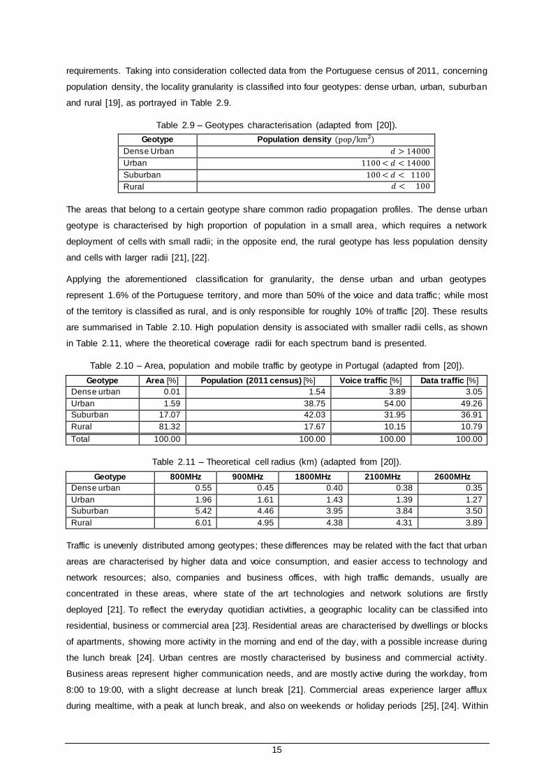
requirements. Taking into consideration collected data from the Portuguese census of 2011, concerning

population density, the locality granularity is classified into four geotypes: dense urban, urban, suburban

and rural [19], as portrayed in Table 2.9.

Table 2.9 – Geotypes characterisation (adapted from [20]).

Geotype Population density (pop/km2)

Dense Urban 𝑑 > 14000

Urban 1100 < 𝑑 < 14000

Suburban 100 < 𝑑 < 1100

Rural 𝑑 < 100

The areas that belong to a certain geotype share common radio propagation profiles. The dense urban

geotype is characterised by high proportion of population in a small area, which requires a network

deployment of cells with small radii; in the opposite end, the rural geotype has less population density

and cells with larger radii [21], [22].

Applying the aforementioned classification for granularity, the dense urban and urban geotypes

represent 1.6% of the Portuguese territory, and more than 50% of the voice and data traffic; while most

of the territory is classified as rural, and is only responsible for roughly 10% of traffic [20]. These results

are summarised in Table 2.10. High population density is associated with smaller radii cells, as shown

in Table 2.11, where the theoretical coverage radii for each spectrum band is presented.

Table 2.10 – Area, population and mobile traffic by geotype in Portugal (adapted from [20]).

Geotype Area [%] Population (2011 census) [%] Voice traffic [%] Data traffic [%]

Dense urban 0.01 1.54 3.89 3.05

Urban 1.59 38.75 54.00 49.26

Suburban 17.07 42.03 31.95 36.91

Rural 81.32 17.67 10.15 10.79

Total 100.00 100.00 100.00 100.00

Table 2.11 – Theoretical cell radius (km) (adapted from [20]).

Geotype 800MHz 900MHz 1800MHz 2100MHz 2600MHz

Dense urban 0.55 0.45 0.40 0.38 0.35

Urban 1.96 1.61 1.43 1.39 1.27

Suburban 5.42 4.46 3.95 3.84 3.50

Rural 6.01 4.95 4.38 4.31 3.89

Traffic is unevenly distributed among geotypes; these differences may be related with the fact that urban

areas are characterised by higher data and voice consumption, and easier access to technology and

network resources; also, companies and business offices, with high traffic demands, usually are

concentrated in these areas, where state of the art technologies and network solutions are firstly

deployed [21]. To reflect the everyday quotidian activities, a geographic locality can be classified into

residential, business or commercial area [23]. Residential areas are characterised by dwellings or blocks

of apartments, showing more activity in the morning and end of the day, with a possible increase during

the lunch break [24]. Urban centres are mostly characterised by business and commercial activity.

Business areas represent higher communication needs, and are mostly active during the workday, from

8:00 to 19:00, with a slight decrease at lunch break [21]. Commercial areas experience larger afflux

during mealtime, with a peak at lunch break, and also on weekends or holiday periods [25], [24]. Within

16

these areas, there are clusters that require specific attention; namely, schools, universities, hospitals,

concert and festival arenas, and sport stadiums.

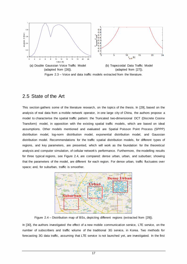
Suggestions for modelling voice and data traffic are presented for the temporal domain, for the duration

of the day, in the literature. Voice traffic is well represented by a Double Gaussian curve; and, data traffic

usage resembles a tree stump shape. In [26], a voice traffic model, referred to as Double Gaussian

Model, is proposed; the model consists of two sections, representing the morning and afternoon peaks,

and is defined by two adjusted gaussian functions, as depicted in Figure 2.3 (a), and expressed by,

𝑎𝑔𝑎𝑢𝑠𝑠 (𝑡) =

{

𝑝1𝑒

−(𝑡−𝑡1)

2

2τ12, 𝑡 < 𝑡𝑙

min (𝑝1𝑒−(𝑡−𝑡1)

2

2τ12; 𝑝2𝑒

−(𝑡−𝑡2)

2

2τ22) , 𝑡 = 𝑡𝑙

𝑝2𝑒−(𝑡−𝑡2)

2

2τ22, 𝑡 > 𝑡𝑙

(2.1)

where:

• 𝑡: shifted hour time, 5 hours earlier, to obtain a simple analytical model;

• 𝑝1 : first gaussian amplitude;

• 𝑡1: morning shifted peak hour;

• τ1: first gaussian deviation;

• 𝑡𝑙: shifted lunch hour;

• 𝑝2 : second gaussian amplitude;

• 𝑡2: afternoon shifted peak hour;

• τ2: second gaussian deviation.

In [27], a data traffic model, referred to as Data Trapezoidal Model, is proposed; the model consists of

two exponentials, with a linear function between them, as depicted in Figure 2.3 (b), and expressed by,

with: 𝑐𝑡𝑟𝑑 = 𝑎𝑡𝑟𝑑1𝑒𝑏𝑡𝑟𝑑1𝑡𝑠ℎ𝑖𝑓𝑡 = 𝑎𝑡𝑟𝑑2𝑒

𝑏𝑡𝑟𝑑2𝑡𝑠ℎ𝑖𝑓𝑡 ;

where:

• 𝑎𝑡𝑟𝑑1: first exponential initial value;

• 𝑏𝑡𝑟𝑑1: first exponential decay factor;

• 𝑡𝑡𝑟𝑑1𝑠ℎ𝑖𝑓𝑡 : first breakpoint shifted hour value;

• 𝑐𝑡𝑟𝑑 : linear constant value;

• 𝑡𝑡𝑟𝑑2𝑠ℎ𝑖𝑓𝑡 : second breakpoint shifted hour value;

• 𝑎𝑡𝑟𝑑2: second exponential initial value;

• 𝑏𝑡𝑟𝑑2: second exponential decay factor;

• 𝑐𝑡𝑟𝑑2: second exponential offset.

The modelling process should resort to nonlinear regression methodologies, as linear regression might

be unable to characterise the intrinsic behaviours of the traffic usage. Nonlinear regression is an iterative

procedure, for adjusting a model, as closely as possible to a data set, by finding fit values for the model’s

parameters. Nonlinear regression is based on the assumption that the scatter of data around the

average curve should follow a normal distribution, as this would indicate that the data follows a

recognisable pattern [28].

𝑓𝑡𝑟𝑎𝑝𝑑𝑎𝑡𝑎 (𝑡𝑠ℎ𝑖𝑓𝑡 ) = {

𝑎𝑡𝑟𝑑1𝑒𝑏𝑡𝑟𝑑1𝑡𝑠ℎ𝑖𝑓𝑡 , 𝑡𝑠ℎ𝑖𝑓𝑡 < 𝑡𝑡𝑟𝑑1𝑠ℎ𝑖𝑓𝑡

𝑐𝑡𝑟𝑑 , 𝑡𝑡𝑟𝑑1𝑠ℎ𝑖𝑓𝑡 ≤ 𝑡𝑠ℎ𝑖𝑓𝑡 ≤ 𝑡𝑡𝑟𝑑2𝑠ℎ𝑖𝑓𝑡

𝑐𝑡𝑟𝑑2 + 𝑎𝑡𝑟𝑑2𝑒𝑏𝑡𝑟𝑑2 𝑡𝑠ℎ𝑖𝑓𝑡 , 𝑡𝑠ℎ𝑖𝑓𝑡 > 𝑡𝑡𝑟𝑑2𝑠ℎ𝑖𝑓𝑡

(2.2)

17

(a) Double Gaussian Voice Traffic Model

(adapted from [26]).

(b) Trapezoidal Data Traffic Model

(adapted from [27]).

Figure 2.3 – Voice and data traffic models extracted from the literature.

2.5 State of the Art

This section gathers some of the literature research, on the topics of the thesis. In [29], based on the

analysis of real data from a mobile network operator, in one large city of China, the authors propose a

model to characterise the spatial traffic pattern: the Truncated two-dimensional DCT (Discrete Cosine

Transform) model, in opposition with the existing spatial traffic models, which are based on ideal

assumptions. Other models mentioned and evaluated are Spatial Poisson Point Process (SPPP)

distribution model, log-norm distribution model, exponential distribution model, and Gaussian

distribution model. Recommendations for the traffic spatial distribution models, for different types of

regions, and key parameters, are presented, which will work as the foundation for the theoretical

analysis and computer simulation, of cellular network's performance. Furthermore, the modelling results

for three typical regions, see Figure 2.4, are compared: dense urban, urban, and suburban; showing

that the parameters of the model, are different for each region. For dense urban, traffic fluctuates over

space; and, for suburban, traffic is smoother.

Figure 2.4 – Distribution map of BSs, depicting different regions (extracted from [29]).

In [30], the authors investigated the effect of a new mobile communication service, LTE service, on the

number of subscribers and traffic volume of the traditional 3G service, in Korea. Two methods for

forecasting 3G data traffic, assuming that LTE service is not launched yet, are investigated. In the first

18

method, the data traffic is estimated based on the real 3G traffic data for a time period. In the other

method, 3G data traffic is separated into two factors: number of subscribers, and data traffic per

subscriber. The first method is considered not appropriate to forecast the data traffic; the latter one,

which separates the 3G traffic volume into two factors, was chosen as the more appropriated method.

In [3], it is introduced a methodology of data analytics and modelling, to evaluate LTE network

performance, based upon traffic measurements and service growth trends. The authors propose an

analytical model, to derive the relationships between measured LTE network Key Performance

Indicators (KPIs), and forecasted network resources. Other methods are referred, and it is mentioned

that there are disadvantages to them, as they cannot analyse how the network resources are

quantitatively consumed, by various applications or users; and, user and service behaviours are lost,

such as user behaviours to consume traffic, diversity of traffic consumption between services, and

seasonality of traffic consumption. In other words, causality was not taken into account; and to overcome

these shortcomings, different model strategies are described. In what concerns the forecast of LTE

traffic and network resources, the model considers four components: trend component, for a long term;

seasonality component, for a given period; burst component, for a significant change from normal trend,

caused by external factors; and, random component. Individual predictions are obtained for each

component, to reflect the variations in behaviours, and user numbers, as different intervals of time are

considered. The method is indicated as able to be generalised, to study other networks such as UMTS.

In [15], the authors propose a novel traffic generation framework for LTE network evolution study, to

obtain heterogeneous application traffic flows, including both typical smartphone applications and

keep-alive messages, generated from always-on applications, and categorise application level traffic

growth forecast. The use of the proposed traffic modelling, is exemplified, with a case study for radio

resource consumption, of voice traffic and keep-alive messages, in a realistic LTE network scenario.

Ultimately, the purpose of the paper is to provide guidelines to LTE network evolution studies. The traffic

generation framework begins with the description of the statistical features of single applications,

including keep-alive messages, and typical internet applications running on smartphone, such as

web-browsing, FTP, e-mail, and buffered video streaming. A general traffic pattern, for a single

smartphone user, is obtained, by focusing on the busy hour, when 8% of overall daily traffic is thought

to be concentrated, and assuming statistical stationarity during this period. The increasing trend of traffic

load of smartphones is considered in scenario development, with the integration of the traffic growth

forecast into the traffic source model, achieved by mapping the growth trend into parameters of each

application traffic source, to assure that the traffic demand can be aligned with the prediction. Table 2.12

shows the forecast of traffic load, per user, per month, and presents the share of each application, based

on measurements from a real LTE network. Simulations are ran in order to evaluate the resource

consumption, in both data plane and control plane, for normal and heavy scenarios. Simulation results

are compared with the measurements of a real network.

In [4], the authors investigate traffic characteristics of popular applications, in Android based

smartphones, by studying the characteristic of these applications, when they are running without user

intervention. In this work, it is presented and discussed various types of applications ; the description of

19

the experiments performed, for diverse data applications, and the results obtained, are presented. An

analysis on traffic characteristics, for applications such as Facebook, Skype, and persistent TCP based

applications, is also presented. For each case, suggestions and guidelines to mend the limitations

identified during the analysis, are enumerated.

Table 2.12 – Application level traffic growth forecast (adapted from [15]).

Year Traffic Load per user

(GB per month)

Percentage [%]

Keep-alive VoIP Web FTP Email Streaming

2016 9.60 0.02 1.80 9.0 12.6 3.0 73.5

2017 13.45 0.01 1.29 8.0 11.2 2.5 77.0

2018 18.82 0.01 0.92 7.0 10.1 2.0 80.0

In [26], the authors analyse the generation of the voice traffic , for the urban area of Lisbon, Portugal.

The modelling is performed for the temporal domain, and the duration of the day, using a

double-gaussian and a trapezoidal function. The first, displays the morning and afternoon rush hour

peaks, and a lunch hour breakpoint; and, for the second, the traffic volume trace has a constant

behaviour for the majority of the day, or for when there are more than two high peaks. In [31], the authors

analyse a urban region, grouping the cells with similar characteristics: cell size, number of channels,

and daily traffic variation trace. Distinct activity areas, to which there is a specific traffic trace, are defined:

urban centre, residential area, and suburban area. It is studied the voice traffic volume along the day,

for workdays and weekends, for two of those regions. In [32], the authors consider the daily data traffic,

from several European cities, when obtaining a data traffic variation profile, for the duration of the day.

The only peak corresponds to the late night period; and, for the lunch hours, there is no decrease in

traffic. In [33], it is obtained a daily data traffic variation, based on the accumulated volume of traffic,

normalised over 24 hours; the busy hour occurs around 9pm. Comparing the average volume of traffic ,

during the weekends and the weekdays, the former is lower than the latter.

In [25], the author addresses diurnal usage profiles for a GSM network. It is stated that the diurnal profile

is important, when dimensioning the network capacity; and that in particular, one should know the busy

hour load, in order to determine the maximum capacity needed in the network. Based on the

measurements performed, the diurnal profile was modelled, for application usage. The usage follows a

typical diurnal profile, with lower intensity at night, and higher during the day; establishing a visible night

and day profile. The diurnal profile of the data volume per application, indicates a distinct usage profile

for the different applications considered. Figure 2.5, depicts the diurnal profile of the data volume, for a

number of applications, presenting the relative data volume per application, over the day, and averaged

over 10-minute intervals.

In [34], the authors present an analysis of data services, based on a 3G data network trace, collected

from one of the largest cellular network service providers in North America. It is stated, this is the first

work to study data service usage patterns, user access behaviours, and network performance issues,

based on measurements from such a large cellular carrier; and, that it differentiates from previous

studies, on the scale of the trace, and the multi-dimension analysis. The paper describes the work data

trace collection methodology, presents the usage characteristics of data services from distinct

perspectives, and concludes with some recommendations for developers and designers of 3G data

20

networks. Device types and diurnal characteristics, are taken into account, in other to characterise the

usage profile; also, data service usage is examined. From the application breakdown, distinct service

types can be observed from the trace, and are used by different users, with different patterns, at different

time periods. More specifically, the work examines different 3G data services diurnal patterns, on a daily

basis, showing different usage patterns between HTTP, MMS and SIP services. Different device types

have distinct application usage profiles; namely, laptop users and mobile phone users. Figure 2.6 shows

the popularity of different applications for each device type, and each bar shows the percentage of users.

Figure 2.5 – Diurnal application usage profile (extracted from [25]).

Figure 2.6 – Usage profiles for each device type (extracted from [34]).

In [23], the authors study the usage of the Google Wi-Fi network, deployed in Mountain View, CA. It is

stated that the aggregate usage of the Google Wi-Fi network, is composed of distinct user populations,

21

characterised by distinct traffic, usage patterns, and mobility. The users are the focus of the study, in

opposition to the focus being the networks themselves. Various classes of active clients, in the Google

Wi-Fi network, are analysed; and, the application workload these clients place on the network , is

characterised. There are distinct peaks on weekdays: morning rush hour, lunch time, and the end of

evening rush hour; the weekends present a smoother behaviour. The dependency with the client device

type, and geographic locality, is also analysed. The usage falls into three classes, based on client device

type, which are the traditional laptop users, fixed-location access devices, and PDA-like smartphone

devices. Each of these classes, for representative time periods, experiences a certain usage according

to the geographic locality, being it on residential, commercial or transportation areas of the city. In what

concerns the overall aggregate network activity, Figure 2.7 shows the number of active clients using the

network, and their average activity time, over 15-minute intervals.

In [35], the authors compile information on mobile traffic, and provide forecasts and trends, for the period

between 2010 and 2020. The focus areas include market trends, mobile broadband services and

applications, key growth markets, spectrum, regulation, technology , and implementation. The report

deals with penetration rates, voice and data traffic, and services that are expected to be used for mobile

networks. Regarding the mobile data traffic, the growing number of mobile devices is shown, considering

tablets, dongles, smartphones, connected devices, and M2M. Based on the segmented categories of

devices, using mobile networks, it is examined the development of a mobile market model, for the

evolution of mobile traffic and services, with future potential. There is a mention to observed data traffic ,

and daily traffic distributions. Global traffic forecasts are considered for different continents and

countries, showing various consumption rates and traffic behaviours , for certain periods of time; also,

some operators’ expectations, and anticipated results, are stated. For Europe, a daily network traffic

consumption is presented; Figure 2.8 depicts the network aggregate traffic profile for Europe.

Figure 2.7 – Usage of the Google Wi-Fi network, for a month (extracted from [23]).

In [24], it is addressed the issue of dimensioning user traffic, in 4G networks; the author introduces the

topic of 4G, and summarises the main appealing subjects and characteristics. Guidelines and

parameters, for the characterisation of user data traffic, are presented. Collected data on user

applications, concerning typical user data traffic, is presented for different time intervals, with

differentiation on the user terminal. Temporal traffic distribution is analysed, by comparing information

on traffic, from residential and business areas. Analysing the DL curve, for the residential case, three

peaks are visible, corresponding to the early morning, the lunch time, and the end of the day; the DL

22

curve, for the business case, has high usage within the work day, with a decrease peak at lunch time.

The residential and business cases are represented by the temporal traffic variation, across the day, for

each hour of the day, as shown in Figure 2.9.

Figure 2.8 – Daily traffic consumption in Europe (extracted from [35]).

Figure 2.9 – Daily traffic profiles (extracted from [24]).

In [36], the authors explore the usage patterns of smartphone applications, via network measurements ,

from a cellular network provider, in the US. This paper addresses the sparse understanding of how,

where, and when, applications are used, compared to traditional web services; presenting results on

applications usage. Regarding user base and geographic area, the work examines the spatial and

temporal prevalence, locality, and correlation, of applications at a national scale; contrary to studying

small areas, or small populations of users. Traffic from distinct applications is identified, based on HTTP

signatures. According to the authors, this study is the first to investigate, the diverse usage behaviours

of individual mobile applications, at scale. The study of usage patterns for the aggregate results, is done

23

from a spatial, temporal, user, and device perspective. An analysis of the diurnal patterns, across various

genres of smartphone applications, is presented; for smartphones, despite diversity, applications that

have high likelihood of being used at the same time, show similarities in usage. News applications are

more frequently used in the early morning, while sports applications are more utilised in the evening.

The authors’ findings suggest that cloud platforms, that host mobile application servers, can leverage

distinct usage patterns in classes of applications, in order to maximise resource utilisation; and, network

operators may optimise their network, for distinct applications, and periods of the day. Figure 2.10 shows

the normalised traffic volume, across the day, at hourly intervals.

In [37], the authors present a study on GSM network utilisation; the experimental analysis focused on

the duration of calls. The traffic peak hour is obtained, for a typical North American GSM network. For

the daily voice traffic curve, there are two peaks; the first one, corresponds to the lunch break; and, the

second peak, corresponds to the time preceding the end of the working day. The study provides

evidence of traffic increase, along the week, from Monday to Friday; and of differentiation of traffic,

between weekdays and weekends. It is introduced a traffic forecasting model, using a regression

analysis. Figure 2.11 represents the measured average durations of calls, for every hour, of the daily

voice traffic, for weekdays and weekends.

Figure 2.10 – Diurnal patterns for different genres of smartphone applications (extracted from [36]).

Figure 2.11 – Traffic in minutes during weekday and weekends (extracted from [37]).

25

Chapter 3

Model Development and

Implementation

3 Model Development and Implementation

This chapter comprises the development framework and the implementation description, used in the

exploratory analysis of the number of active users and traffic usage, and to obtain the models for the

statistical characterisation of traffic usage, from a live cellular network. The data is structured and

analysed. The models are compared and ranked based on goodness of fit statistics’ criteria. The

regression results are found at the end.

26

3.1 Data Collection

Studying and gaining a broader understanding of how impactful people’s daily lives , and routines, are

in application utilisation, device preferences, and network resource demands , is relevant for network

optimisation. Data from live cellular mobile networks, can be used to characterise usage behaviours ,

from a statistical viewpoint, in order to gather recommendations and guidelines for efficient resource

usage. A data set, collected from a mobile network, can be divided between a training set and a

validation set, if the number of observations is large enough. The training set is used in the fitting

process, to find prediction models; and, the validation set is used to validate the fitted models, with an

independent set of observations. One should pay attention and check if the data was carefully selected,

in order to avoid introducing systematic errors, or overly fitting the models to a very specific setting.

3.1.1 Training Data Set

The input data set, to function as training set, was collected at the core level of the Vodafone Portugal

network, in Portugal, Lisbon, and contains 583885 observations. The observation period, from

2016/03/12 to 2016/04/19, includes 39 days, in which 26 are weekdays, 12 are weekend days, and 1 is

a national holiday day. The national holiday days are considered as weekend days.

Sunrise and sunset time changes daily, due to the variations of the daytime, which is the period a given

point of the Earth experiences natural light, making the day length fluctuate. The length of day is the

elapsed time between sunrise and sunset. For the Lisbon area, the length of day increases from

2016/03/12 to 2016/04/19, going from 11h47m of daytime, to 13h21m. During this observation period,

on 2016/03/27, a Sunday, a time shift occurs, with clocks turning forward one hour.

Table 3.1 – Length of day for March and April, for the Lisbon area.

Date Sunrise Sunset Length of day

2016/03/12 06:52 18:39 11h47min

2016/03/26 06:31 18:53 12h22min

Spring Time Shift

2016/03/27 07:29 19:54 12h24 min

2016/04/01 07:21 19:59 12h37 min

2016/04/19 06:55 20:16 13h21 min

The input spreadsheet file is organised into 9 fields: date, time, APP_GROUP, DEV_TYPE, OP_SYS,

USERS, DOWNLOAD, and UPLOAD:

• The date and time fields define the observation timestamp. The time field takes values from

00:00 to 23:00; and, the time unit is expressed in top-of-the-hour.

• The APP_GROUP field designates the different application labels; data applications with similar

features are identified, in the spreadsheet, with the same application label.

• The DEV_TYPE field designates the type of device used.

• The OP_SYS field designates the type of operating systems used by the device.

• The USERS field designates the number of distinct Mobile Subscriber Integrated Service Digital

Network Numbers (MSISDNs). The MSISDN is the telephone number associated with a SIM,

27

and identifies the mobile subscriber.

• The DOWNLOAD field indicates the traffic usage, in the download link, measured in Bytes.

• The UPLOAD field indicates the traffic usage, in the upload link, measured in Bytes.

The training set information is summarised in Table 3.2.

Table 3.2 – Training set description.

Classes Subclasses Observations Observations [%]

APP_GROUP

E-Mail 55259 9.46

File Systems 32694 5.60

File Transfer 54152 9.27

Games 45877 7.86

Instant Messaging 56177 9.62

Other 59712 10.23

P2P 46252 7.92

Streaming 52996 9.08

Terminal Transactions 62340 10.68

VoIP 56140 9.61

Web Applications 62129 10.64

Legacy Protocols 157 0.03

Total 583885 100.00

DEV_TYPE

Hotspots 43093 7.38

Others 93327 15.98

Pens 57150 9.79

Routers 80976 13.87

Smartphone 212324 36.36

Tablet 97015 16.62

Total 583885 100.00

OP_SYS

Android 157027 26.89

Blackberry 33635 5.76

Others 211669 36.25

iOS 78601 13.46

Symbian 27732 4.75

Windows 75221 12.88

Total 583885 100.00

Data entries of applications with similar features, are gathered and assigned, to the same APP_GROUP

label designation. The APP_GROUP applications are: E-mail; File Transfer (FiTr); Games; Instant

Messaging (InMe); M2M; Other; P2P; Streaming; VoIP; Web Applications (WebAp); and, Legacy

Protocols. M2M groups the data entries from Terminal Transactions and File Systems observations.

The Legacy Protocols will be left out since they only represent 0.03% of the observations, which is a

negligible number and would not provide meaningful results.

The DEV_TYPE devices are: Hotspots; Others; Pens & Datacards, which in the future will be referred

to as Pens; Routers; Smartphone; and, Tablet. Hotspots are Wi-Fi terminals of high mobility, that allow

connectivity for many devices at the same time [38], while Pens only allow connectivity for one device

[39]. Routers are Wi-Fi fixed terminals, that allow connectivity for many devices at the same time [40].

The OP_SYS operating systems are: Android; Others; Windows; iOS; BlackBerry; and, Symbian.

BlackBerry and Symbian will be left out, since they both have a small representation in the data set, and

are neglectable in comparison with other operating systems.

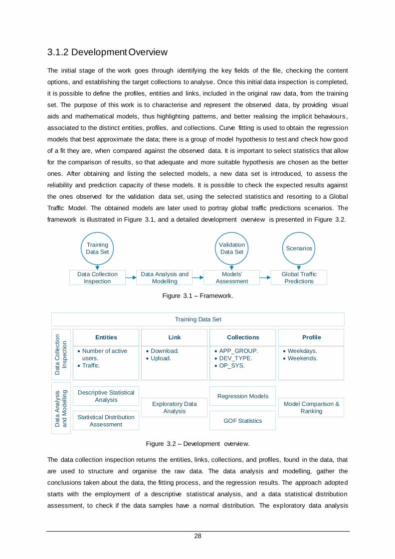
28

3.1.2 Development Overview

The initial stage of the work goes through identifying the key fields of the file, checking the content

options, and establishing the target collections to analyse. Once this initial data inspection is completed,

it is possible to define the profiles, entities and links, included in the original raw data, from the training

set. The purpose of this work is to characterise and represent the observed data, by providing visual

aids and mathematical models, thus highlighting patterns, and better realising the implicit behaviours ,

associated to the distinct entities, profiles, and collections. Curve fitting is used to obtain the regression

models that best approximate the data; there is a group of model hypothesis to test and check how good

of a fit they are, when compared against the observed data. It is important to select statistics that allow

for the comparison of results, so that adequate and more suitable hypothesis are chosen as the better

ones. After obtaining and listing the selected models, a new data set is introduced, to assess the

reliability and prediction capacity of these models. It is possible to check the expected results against

the ones observed for the validation data set, using the selected statistics and resorting to a Global

Traffic Model. The obtained models are later used to portray global traffic predictions scenarios. The

framework is illustrated in Figure 3.1, and a detailed development overview is presented in Figure 3.2.

Data Collection

Inspection

Data Analysis and

Modelling

Models

Assessment

Global Traffic

Predictions

Training

Data Set

Validation

Data Set Scenarios

Figure 3.1 – Framework.

Data

Co

llectio

n

Insp

ectio

n

Data

Ana

lysis

and

Mo

dellin

g

•Number of active

users.

•Traffic.

Entities

•Number of active

users.

•Traffic.

Entities

•APP_GROUP.

•DEV_TYPE.

•OP_SYS.

Collections

•APP_GROUP.

•DEV_TYPE.

•OP_SYS.

Collections

•Weekdays.

•Weekends.

Profile

•Weekdays.

•Weekends.

Profile

•Download.

•Upload.

Link

•Download.

•Upload.

Link

Descriptive Statistical

AnalysisExploratory Data

AnalysisStatistical Distribution

Assessment

Regression Models

GOF Statistics

Model Comparison &

Ranking

Training Data Set

Figure 3.2 – Development overview.

The data collection inspection returns the entities, links, collections, and profiles, found in the data, that

are used to structure and organise the raw data. The data analysis and modelling, gather the

conclusions taken about the data, the fitting process, and the regression results. The approach adopted

starts with the employment of a descriptive statistical analysis, and a data statistical distribution

assessment, to check if the data samples have a normal distribution. The exploratory data analysis

29

makes use of graphical and numerical results for an accessible and compact representation of the data

related to the different collections, profiles, entities, and links. The fitting process, uses a model

catalogue that lists the models, used as the set of hypotheses for the regression process. The list of

tested models has 8 possible models, and each model is composed of one or more sections,

represented by linear, exponential, and gaussian equations.

The regression models are obtained by estimating the coefficients of each section, by means of a

nonlinear least-squares algorithm, while ensuring continuity between the sections , and the initial and

final points of the model. To decide on the better regression models, goodness of fit statistics are used

to implement a criteria, for comparing and ranking the hypothesis, on how well they approximate the

data, and respective average curves. The validation data set is used for the models’ and predictions ’

assessments. With the listing of the selected models, the models’ assessment is performed to test the

fitting, of the obtained regression models, with a new data set. The Global Traffic Model, set from 00:00

to 24:00, is used to show the expected traffic usage, to compare against the observed one; and is used

for scenarios’ predictions.

To maintain the confidentiality of the collected information, the data is presented normalised.

3.1.3 Descriptive Statistical Analysis

For each 𝑖𝑡ℎ top of the hour, or observation, there are 𝑁𝑆 samples of data. The average of the 𝑖𝑡ℎ

observation is defined as [41],

μ𝑖 =1

𝑁𝑆∑ 𝑦𝑗

𝑁𝑆

𝑗 =1 (3.1)

where:

• 𝑁𝑆: number of samples;

• 𝑦𝑗 : 𝑗𝑡ℎ sample.

Each μ𝑖value defines a point of the average curve, and has a global average defined as,

μ̅ =1

𝑁∑ μ𝑖

𝑁

𝑖=1 (3.2)

where:

• 𝑁: number of observations.

The standard deviation, associated with each μ𝑖value, quantifies the sample dispersion as [41],

σ𝑖 = √1

𝑁𝑆∑ (𝑦𝑗 − μ𝑖)

2𝑁𝑆

𝑗=1 (3.3)

The average standard deviation about the average curve is defined as,

σ̅ = √1

𝑁∑ σ𝑖

2𝑁

𝑖=1

(3.4)

The normalisation of data, and average curves, is performed by dividing the sample values, by a

normalisation constant. The normalised observed values are defined as,

30

𝑦𝑗 𝑁𝑜𝑟𝑚=

𝑦𝑗

𝑦𝑐𝑜𝑛𝑠𝑡 (3.5)

where:

• 𝑦𝑐𝑜𝑛𝑠𝑡 : normalisation constant.

To weigh the results, with respect to the share each input has in the data set, the weighted average is,

𝑅𝑤 = ∑ 𝑤𝑛 ∙ 𝑅𝑛 𝑁𝑛

𝑛=1 (3.6)

where:

• 𝑛: case index;

• 𝑁𝑛: number of cases;

• 𝑤𝑛 : weight;

• 𝑅𝑛 : input ratios.

The percent change measures the relative increase, or decrease, between the reference and the

observed inputs,

Δ𝑅𝑛 [%] =𝑅𝑜𝑏𝑠 − 𝑅𝑟𝑒𝑓

𝑅𝑟𝑒𝑓×100 (3.7)

where:

• 𝑅𝑟𝑒𝑓 : reference input;

• 𝑅𝑜𝑏𝑠 : observed input.

3.1.4 Goodness of Fit Tests

There are two possible outcomes as a result of a hypothesis, either the result is consistent with the

hypothesis, which is retained, or in case of inconsistency, the hypothesis is rejected. One cannot prove

an hypothesis, one can only falsify or disprove an hypothesis [42]. To know the underlying distribution

of data samples, one tests for goodness of fit, to check if a hypothesised distribution is rejected or not.

The null hypothesis is the hypothesis under test, and the hypothesis test result either states that the null

hypothesis was, or was not, rejected at a α level of significance [41]. The Lilliefors Test for Normality is

especially designed to assess if the statistical distribution is a normal distribution. The null hypothesis,

𝐻0, is that the sample comes from a normal distribution. This test performs like the Kolmogorov-Smirnov

test, but the Lilliefors test standardises the data using the sample estimates of the average, and of the

standard deviation. The Lilliefors test measures the goodness of fit between the empirical Cumulat ive

Distribution Function (CDF) of the data, and the theoretical CDF of the hypothesised distribution, with

parameters estimated from the data. The Lilliefors test rejects the null hypothesis at a level α of

significance, if 𝐷𝐿𝑖𝑙𝑙𝑖𝑒𝑓𝑜𝑟𝑠 is larger than the critical value [43], [44], and [45]. The Lilliefors’ test statistic is,

𝐷𝐿𝑖𝑙𝑙𝑖𝑒𝑓𝑜𝑟𝑠 = max𝑋|�̂�𝑋(𝑥)− 𝐹𝑋(𝑥)| (3.8)

where:

• 𝐹𝑋 : empirical CDF;

• 𝐹𝑋 : theoretical CDF (hypothetical distribution).

The lillietest MATLAB command [43], returns a test decision for a α level of significance. The hypothesis

test result, either takes the value 1, which indicates the rejection of the null hypothesis, or takes the

value 0, which indicates a failure to reject the null hypothesis.

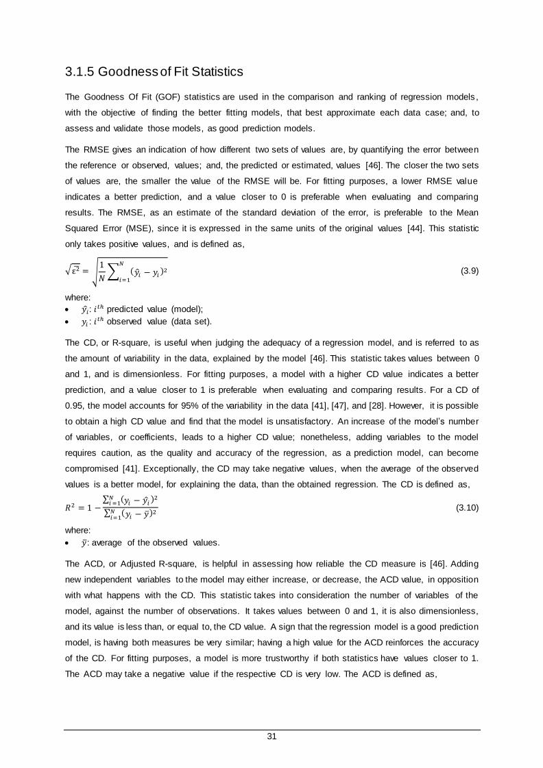
31

3.1.5 Goodness of Fit Statistics

The Goodness Of Fit (GOF) statistics are used in the comparison and ranking of regression models ,

with the objective of finding the better fitting models, that best approximate each data case; and, to

assess and validate those models, as good prediction models.

The RMSE gives an indication of how different two sets of values are, by quantifying the error between

the reference or observed, values; and, the predicted or estimated, values [46]. The closer the two sets

of values are, the smaller the value of the RMSE will be. For fitting purposes, a lower RMSE value

indicates a better prediction, and a value closer to 0 is preferable when evaluating and comparing

results. The RMSE, as an estimate of the standard deviation of the error, is preferable to the Mean

Squared Error (MSE), since it is expressed in the same units of the original values [44]. This statistic

only takes positive values, and is defined as,

√ε2̅ = √1

𝑁∑ (�̂�𝑖 − 𝑦𝑖 )

2𝑁

𝑖=1

(3.9)

where:

• 𝑦𝑖: 𝑖𝑡ℎ predicted value (model);

• 𝑦𝑖 : 𝑖𝑡ℎ observed value (data set).

The CD, or R-square, is useful when judging the adequacy of a regression model, and is referred to as

the amount of variability in the data, explained by the model [46]. This statistic takes values between 0

and 1, and is dimensionless. For fitting purposes, a model with a higher CD value indicates a better

prediction, and a value closer to 1 is preferable when evaluating and comparing results. For a CD of

0.95, the model accounts for 95% of the variability in the data [41], [47], and [28]. However, it is possible

to obtain a high CD value and find that the model is unsatisfactory. An increase of the model’s number

of variables, or coefficients, leads to a higher CD value; nonetheless, adding variables to the model

requires caution, as the quality and accuracy of the regression, as a prediction model, can become

compromised [41]. Exceptionally, the CD may take negative values, when the average of the observed

values is a better model, for explaining the data, than the obtained regression. The CD is defined as,

𝑅2 = 1 −∑ (𝑦𝑖 − 𝑦𝑖 )

2𝑁𝑖 =1

∑ (𝑦𝑖 − 𝑦)2𝑁

𝑖=1

(3.10)

where:

• 𝑦: average of the observed values.

The ACD, or Adjusted R-square, is helpful in assessing how reliable the CD measure is [46]. Adding

new independent variables to the model may either increase, or decrease, the ACD value, in opposition

with what happens with the CD. This statistic takes into consideration the number of variables of the

model, against the number of observations. It takes values between 0 and 1, it is also dimensionless,

and its value is less than, or equal to, the CD value. A sign that the regression model is a good prediction

model, is having both measures be very similar; having a high value for the ACD reinforces the accuracy

of the CD. For fitting purposes, a model is more trustworthy if both statistics have values closer to 1.

The ACD may take a negative value if the respective CD is very low. The ACD is defined as,

32

𝑅𝑎𝑑𝑗2 = 1 −

(1 − 𝑅2)(𝑁 − 1)

𝑁 − 𝑃 − 1 (3.11)

where:

• 𝑃: number of predictors (model coefficients).

When evaluating and comparing different regression models, with similar goodness of fit statistics

results, the coefficient’s Confidence Interval (CI) can be a deciding factor. The coefficients’ CIs give a

sense of the trust one can put, in the values obtained for the coefficients. The further apart the lower

and upper bounds are, the less assurance one can have on the results; regression models that are

characterised by very wide CIs should be disregarded. For fitting purposes, a narrow interval is

preferable, and indicates more adequate coefficients.

The RMSE and the CD, are not the sole indicators of how well a regression model fits the data, and

must be complemented by the ACD. The most favourable scenario is to have the regression model

show low RMSE; high and similar, CD and ACD; and, narrow CIs widths. A good prediction model is

one which is able to adequately approximate the set of observations. It is possible that many reasonable

predictions can be obtained, so deciding on the more suitable one, also should have into consideration

the underlying behaviour aspects of the data. These statistics and recommendations, are used as

criteria and guidelines, in deciding, out of a model catalogue, which model better fits each data case.

3.2 Development Conditions and Considerations

3.2.1 Data Collection Analysis

Three collections, out of the original data collection, are studied and analysed separately, with the

objective of obtaining models able to describe and predict the underlying data behaviours. The first is

the Applications (App) collection, and refers to the APP_GROUP data; the second is the Devices (Dev)

collection, and refers to the DEV_TYPE data; and the third is the Operating Systems (OpS) collection,

and refers to the OP_SYS data: 𝑐 = {𝐴𝑝𝑝 , 𝐷𝑒𝑣, 𝑂𝑝𝑆}. The entities in analysis are the number of active

users, and traffic usage: 𝐸 = {𝑁𝑢 , 𝑇[𝐺𝐵]}. Both entities, 𝐸, are defined in terms of an hour of the day, ℎ; a

day, 𝑑; a collection, 𝑐, with 𝑛 cases; a profile, 𝑝; a link, 𝑙; as: 𝐸(ℎ, 𝑑, 𝑐|𝑛, 𝑝, 𝑙). In a period of a day, there

are 24 top of the hours: ℎ = {1, … , 24}. Each collection is sorted into two profiles, weekdays and

weekends, with 𝑝 = {𝑊𝐷,𝑊𝐸}; and, 𝑊𝐷|𝑑 = {1, … , 26}, and 𝑊𝐸|𝑑 = {1, … , 13}. Furthermore, traffic

usage is considered for both DL and UL links, 𝑙 = {𝐷𝐿,𝑈𝐿}. The App collection has 10 cases, the Dev

collection has 6 cases, and the OpS collection has 4 cases:

𝑐 = 𝐴𝑝𝑝, 𝑛 = {𝐸𝑚𝑎𝑖𝑙 , 𝐹𝑖𝑇𝑟, 𝐺𝑎𝑚𝑒𝑠 , 𝐼𝑛𝑀𝑒 ,𝑀2𝑀, Other, P2P, 𝑆𝑡𝑟𝑒𝑎𝑚𝑖𝑛𝑔, 𝑉𝑜𝐼𝑃,𝑊𝑒𝑏𝐴𝑝 };

𝑐 = 𝐷𝑒𝑣, 𝑛 = {𝐻𝑜𝑡𝑠𝑝𝑜𝑡𝑠 , 𝑂𝑡ℎ𝑒𝑟𝑠 , 𝑃𝑒𝑛𝑠 , 𝑅𝑜𝑢𝑡𝑒𝑟𝑠, 𝑆𝑚𝑎𝑟𝑡𝑝ℎ𝑜𝑛𝑒 , 𝑇𝑎𝑏𝑙𝑒𝑡};

𝑐 = 𝑂𝑝𝑆 , 𝑛 = {𝐴𝑛𝑑𝑟𝑜𝑖𝑑 , 𝑂𝑡ℎ𝑒𝑟𝑠,𝑊𝑖𝑛𝑑𝑜𝑤𝑠, 𝑖𝑂𝑆}.

Four scenarios are established, {𝑊𝐷,𝐷𝐿}; {𝑊𝐷, 𝑈𝐿}; {𝑊𝐸 , 𝐷𝐿}; and, {𝑊𝐸, 𝑈𝐿}.

33

Originally, the data set is a record of data entries for 39 days. After retrieving the data entries for each

day, and each top of the hour, it is possible to start structuring the raw data set, into the different data

collections, profiles, entities, and cases. Figure 3.3 depicts the normalised total traffic for the 39 day

observation period, distinguishing WD from WE. Once the data is structured, one gains access to all

collections, profiles, entities, and cases, independently. The difference in behaviour and traffic load,

between WD and WE, is noticeable from inspecting the figure.

Figure 3.3 – Traffic usage data observations over 39 days, from 2016/03/12 to 2016/04/19.

Figure 3.4 (a) displays the normalised DL traffic usage, for the Streaming case, for both WD and WE.

The temporal window represents a day period, with a precision of a measurement of one hour, and 24

top of the hour observations. Each hour is defined by its top of the hour; and, one observation designates

the samples for a top of the hour. There are 24 observations in total, and each has as many samples as

the profile‘s number of days; WD have 26 samples per observation, and WE have 13.

The average curve is obtained by averaging the samples for each top of the hour. For each top of the

hour, samples have a different dispersion pattern about the average, quantified by the standard

deviation, see Figure 3.4 (b). The average standard deviation is the outcome of averaging the standard

deviations of each observation. The display of the average curve, and the average standard deviation

region about the average, provide insight on the data for each observation, and over the day period.

The data samples, of each observation, only take positive values, due to the nature of the data of the

three entities. Figure 3.4 (b) displays the average curve, and the sample scatter about the average, for

the Streaming case, for WD and DL. The data and the average curve experience a shift translation, and

its values are normalised; normalisation is done in reference to the maximum value of the observations.

(a) Download Data Observations. (b) Weekdays Download.

Figure 3.4 – APP_GROUP Streaming.

34

3.2.2 Data Statistical Distribution Assessment

It is important to understand how well behaved the distribution of scatter about the average is, and if

one can consider the scatter, of each hour, to have a normal distribution. It is more straightforward to fit,

and find, a good regression model, if the scatter distribution about the average, for each top of the hour,

is well-behaved. Examining the scatter distribution about the average against the normal distribution,

for each top of the hour, gives an indication of how well-behaved the samples about the average are.

The normal distribution is symmetric about the average; and, for any normal distribution, there is a 68.3%

chance a sample is within the one standard deviation region about the average; a 95.45% chance a

sample is within the two standard deviation region; and a 99.73% chance a sample is within the three

standard deviation region [41]. For each top of the hour, one assesses if the statistical distribution of the

samples about the average is normal. In truth, the samples only take positive values, therefore the more

appropriate distribution to use is the truncated normal distribution; however, the normal distribution can

be used since, while a sample from the normal distribution can take a positive or negative value, if the

average is large enough, in comparison with the standard deviation, then the chance of finding a sample

with negative value, within the three standard deviation region, is negligible [48]. The Lilliefors goodness

of fit test is used to assess if the samples’ scatter about the average has a normal distribution. The

Lilliefors test is performed for a 5% level of significance.

A histogram is a column diagram, and a visual inspection of the graph provides an initial understanding

of the data distribution about the average [49], in anticipation of the goodness of fit normality tests. For

the Streaming case, two visual aids are provided to illustrate a good, Figure 3.5 (a), and a worst, Figure

3.5 (b), situations of data distribution about the average. For WD and DL, the percentage of non-rejected

decisions is 83.33%; and, for WD and UL, the percentage of non-rejected decisions is 41.67%.

(a) Weekdays Download. (b) Weekdays Upload.

Figure 3.5 – APP_GROUP Streaming Histogram.

The Lilliefors test is performed for a 5% level of significance. The Lilliefors test assesses the normality

of the traffic distribution about the average traffic curve, for each case, for all four scenarios, and three

collections. The test decisions, which return a rejection of the null hypothesis, with a test statistic value

surpassing less than 10% of the critical value, are considered as failure to reject the null hypothesis. For

WD the critical value is 0.1698, and for WE is 0.2333. The percentages of non-rejected decisions, in the

-250 -200 -150 -100 -50 0 50 1000

10

20

30

40

50

Streaming Download Histogram

Download Traffic [GB]

Num

ber

of

Sam

ple

s

-30 -25 -20 -15 -10 -5 0 5 10 150

5

10

15

20

25

30

35

40

45

Streaming Upload Histogram

Upload Traffic [GB]

Num

ber

of

Sam

ple

s

35

assessment at 5% level, of the goodness of fit to the normal distribution, using the Lilliefors goodness

of fit test, are presented in Table 3.3, Table 3.4, and Table 3.5. The weighted average is the product

between the weight of the traffic, for each case, and the respective result for the Lilliefors test.

Regarding the App collection, the better overall results are achieved for VoIP, and the worst ones for

Other. The lowest percentage of non-rejected decisions is obtained for Other, UL and WD; and, for

Streaming, UL and WE; and, the highest percentage of non-rejected decisions is obtained for M2M, DL

and WE; and for VoIP, UL and WE. The weighted average of the percentages of non-rejected decisions

has a minimum of 74.15%, for UL and WD, and a maximum of 93.25%, for DL and WE. Regarding the

Dev collection, the better overall results are achieved for the Routers, and the worst ones for Others.

The lowest percentage of non-rejected decisions is obtained for the Routers, UL and WE; and, the

highest percentage of non-rejected decisions is obtained for Others, DL and WD. The weighted average

of the percentages of non-rejected decisions has a minimum of 77.32%, for UL and WD, and a maximum

of 94.71%, for UL and WE. Regarding the OpS collection, the better overall results are achieved for iOS,

and the worst ones for Windows. The lowest percentage of non-rejected decisions is obtained for

Windows, UL and WD; and, the highest percentage of non-rejected decisions is obtained for Android

and iOS, UL and WE. The weighted average of the percentages of non-rejected decisions has a

minimum of 76.46%, for DL and WD, and a maximum of 93.70%, for UL and WE.

Table 3.3 – Percentages of non-rejected decisions, for APP_GROUP, in the assessment at 5%

level of significance, to the normal distribution, using the Lilliefors test.

App Collection

Non-rejected decisions [%]

Download Upload

Weekdays Weekends Weekdays Weekends

(1) E-Mail 70.83 83.33 79.17 87.50

(2) FiTr 45.83 91.67 70.83 83.33

(3) Games 45.83 62.50 79.17 91.67

(4) InMe 70.83 79.17 83.33 91.67

(5) M2M 87.50 100.00 75.00 91.67

(6) Other 54.17 91.67 50.00 79.17

(7) P2P 83.33 95.83 95.83 91.67

(8) Streaming 83.33 91.67 41.67 50.00

(9) VoIP 95.83 83.33 95.83 100.00

(10) WebAp 87.50 95.83 87.50 87.50

Weighted Average 80.65 93.25 74.15 78.64

Table 3.4 – Percentages of non-rejected decisions, for DEV_TYPE, in the assessment at 5% level

of significance, to the normal distribution, using the Lilliefors test.

Dev Collection

Non-rejected decisions [%]

Download Upload


(1) Hotspots 87.50 87.50 58.33 87.50

(2) Others 50.00 95.83 70.83 87.50

(3) Pens 91.67 91.67 79.17 91.67

(4) Routers 87.50 91.67 87.50 100.00

(5) Smartphone 79.17 91.67 79.17 95.83

(6) Tablet 95.83 95.83 58.33 91.67


36

Table 3.5 – Percentages of non-rejected decisions, for OP_SYS, in the assessment at 5% level of

significance, to the normal distribution, using the Lilliefors test.

OpS Collection

Non-rejected [%]

Download Upload


(1) Android 79.17 91.67 83.33 95.83

(2) Others 70.83 87.50 70.83 91.67

(3) Windows 62.50 79.17 20.83 50.00

(4) iOS 83.33 91.67 87.50 95.83


The weighted average, of the percentages of non-rejected decisions, is superior to 74%, for the App

collection; to 77%, for the Dev collection; and, to 76%, for the OpS collection.

3.3 Exploratory Data Analysis

Exploratory data analysis makes use of graphical and numerical results , to show previously inaccessible

information, from the original raw data. The visual aids and tables allow for a compact representation,

and an easy consultation, of the disclosed information. The entities in analysis are the Number of Active

Users (NU) and traffic usage.

3.3.1 Data Ratios

The entity, for the ℎ hour, in a 𝑑 day, for a 𝑛 case, is the result of combining all file entries in those

conditions. The entity, for the 12:00 top of the hour, for the first day of WD set, for DL, when considering

the App collection, for the Streaming case, is as follows,

𝐸(ℎ = 12,𝑑 = 1, 𝑐 = 𝐴𝑝𝑝,𝑝 = 𝑊𝐷, 𝑙 = 𝐷𝐿, 𝑛 = 8) (3.12)

The entity, for the ℎ hour, in a 𝑑 day, is the result of combining all 𝑛 case contributions in those conditions.

The entity, for the 12:00 top of the hour, for the first day of WD set, for DL, when considering the App

collection for all 10 cases, is as follows,

𝐸(ℎ = 12,𝑑 = 1, 𝑐 = 𝐴𝑝𝑝,𝑝 = 𝑊𝐷, 𝑙 = 𝐷𝐿)

=∑ 𝐸(ℎ = 12, 𝑑 = 1,𝑐 = 𝐴𝑝𝑝|𝑛,𝑝 = 𝑊𝐷, 𝑙 = 𝐷𝐿 )

𝑁𝑛

𝑛=1

(3.13)

where:

• 𝑁𝑛: number of cases.

The Total Entity, for a full day, considers all 𝑛 cases contributions, for each one of the 24 top of the

hours, for the chosen collection, profile, and link. The entity, for all 24 top of the hour, for the first day of

WD set, for DL, when considering the App collection with 10 cases, is as follows,

𝐸(𝑑 = 1,𝑐 = 𝐴𝑝𝑝,𝑝 = 𝑊𝐷, 𝑙 = 𝐷𝐿) =∑∑𝐸(ℎ, 𝑑 = 1, 𝑐 = 𝐴𝑝𝑝|𝑛,𝑝 = 𝑊𝐷, 𝑙 = 𝐷𝐿)

𝑁𝑛

𝑛=1

𝑁𝐻

ℎ=0

(3.14)

where:

37

• 𝑁𝐻: number of hours.

The Average Hour Weight, for the ℎ hour, is the average over all days of the profile set, for all 𝑛 cases

contributions, for the ℎ top of the hour, pondered to all cases and all hours contributions of that day. The

ratio, for the 𝐸 entity, for the 12:00 top of the hour, pondered to all 24 top of the hour, for each 𝑑 day of

WD set, for DL, when considering the App collection with 10 cases, is,

𝑤ℎ=12𝐸̅̅ ̅̅ ̅̅ ̅̅ =

1

𝑁𝐷[∑

∑ 𝐸(ℎ = 12, 𝑑, 𝑐 = 𝐴𝑝𝑝|𝑛, 𝑝 = 𝑊𝐷, 𝑙 = 𝐷𝐿)𝑁𝑛𝑛=1

∑ ∑ 𝐸(ℎ, 𝑑, 𝑐 = 𝐴𝑝𝑝|𝑛, 𝑝 = 𝑊𝐷, 𝑙 = 𝐷𝐿)𝑁𝑛𝑛=1

𝑁𝐻ℎ=0

𝑁𝐷

𝑑=1

] (3.15)

where:

• 𝑁𝐷: number of days.

This quantifies the average weight each hour has in the duration of one day. All collections, for the same

entity, profile, and link, have equal hour weights. For the graphical representation, the sum of all top of

the hour contributions (columns) adds up to 100%.

The Entity Average Hourly Ratio, for the 𝑛 case, is the average over all days of the profile set, of one

case contribution, for the ℎ top of the hour, pondered to all cases contributions of that ℎ top of the hour

for each day. The ratio, for the 𝐸 entity, for the 12:00 top of the hour, the Streaming case is pondered to

all cases, for each of the days of WD set, for DL, when considering the App collection, is,

𝑤𝐻 ℎ=12,𝑛=8𝐸̅̅ ̅̅ ̅̅ ̅̅ ̅̅ ̅̅ ̅̅ ̅ =

1

𝑁𝐷[∑

𝐸(ℎ = 12, 𝑑,𝑐 = 𝐴𝑝𝑝, 𝑝 = 𝑊𝐷, 𝑙 = 𝐷𝐿, 𝑛 = 8)

∑ 𝐸(ℎ = 12, 𝑑, 𝑐 = 𝐴𝑝𝑝|𝑛, 𝑝 = 𝑊𝐷, 𝑙 = 𝐷𝐿)𝑁𝑛𝑛=1

𝑁𝐷

𝑑=1

] (3.16)

This quantifies the average weight each case has for each hour, for the 24 top of the hours. Each

collection, for each entity and selected profile set, link , and case, has a different hourly weights

distribution. For the graphical representation, the sum of each top of the hour contributions (column)

adds up to 100%.

The Entity Average Daily Ratio, for the 𝑛 case, uses the average weight of each hour, and the average

weight of a case for that hour, to obtain the weight of each case, per hour, for a day; it is the Entity

Weighted Average Hourly Ratio, for the 𝑛 case. The ratio, for the 𝐸 entity, for the 12:00 top of the hour,

and the Streaming case, for the selected profile set, and link, when considering the App collection, is,

𝑤𝐷 ℎ=12,𝑛=8𝐸̅̅ ̅̅ ̅̅ ̅̅ ̅̅ ̅̅ ̅̅ ̅ = 𝑤ℎ=12

𝐸̅̅ ̅̅ ̅̅ ̅̅ ∙ 𝑤𝐻 ℎ=12,𝑛=8𝐸̅̅ ̅̅ ̅̅ ̅̅ ̅̅ ̅̅ ̅̅ ̅ (3.17)

This quantifies the average weight each case, in each top of the hour, has in the duration of one day.

Each collection, for each entity, selected profile set, link, and case, has a different daily weights

distribution. For the graphical representation, the sum of all top of the hour contributions (columns) adds

up to 100%.

For a 𝑛 case, the Entity Average Aggregated Daily Ratio, combines all Entity Weighted Average Daily

Ratios, obtained for the duration of one day. The ratio, for the 𝐸 entity, for all 24 top of the hour, and the

Streaming case, for the selected profile set, and link, when considering the App collection, is,

38

𝑤𝑛=8𝐸̅̅ ̅̅ ̅̅ ̅ = ∑𝑤𝐷 ℎ,𝑛=8

𝐸̅̅ ̅̅ ̅̅ ̅̅ ̅̅ ̅

𝑁𝐻

ℎ=0

(3.18)

This quantifies the average weight each case has in the duration of one day. For the graphical

representation, the sum of all contributions (columns) adds up to 100%.

The data set is assessed for the NU and the traffic usage, for both DL and UL, using the previous ly

explained data ratios, with results expressed in percentage. The results display the share of the entity

related to each top of the hour, in the period of a day; the share of the entity each case of a collection

shows, for each one of the 24 top of the hours; the share of the entity associated to a certain case of a

collection, weighted to a specific top of the hour; and, for the entire day, the share of the entity which

portrays a certain case of a collection.

3.3.2 Global Results

The distribution of each entity, along the period of 24 hours, for both WD and WE, is analysed. The hour

weights for each entity and a selected profile, either WD or WE, yield the same results for all collections .

Regarding WD, see Figure 3.6, all entities show an increase in the morning; the NU, shows a decrease

in the afternoon, starting around 19:00, and throughout the night and early morning, until hitting a

minimum between the hours of 3 and 6 in the morning, also, it takes the highest values between the

hours of 9 and 20, with a maximum around 14:00 and 18:00; the DL traffic, shows a very steep

progression between the hours of 7 and 10, and, only shows a decrease in the late night, after midnight,

and hits minimum values between the hours of 3 and 6 in the morning, also, it takes the highest values

between the hours of 11 and 23, with peaks at 18:00 and 22:00; the UL traffic, shows a steady

progression between the hours of 7 and 10, and, starts showing a decrease after 19:00, and hits

minimum values between the hours of 3 and 6 in the morning, also, it takes the highest values between

the hours of 11 and 22, with a maximum around 17:00.

Figure 3.6 – Weekdays Hour Weights.

Regarding WE, the NU, shows a more gradual increase in the morning, starting around 8:00, and, starts

to slowly decrease around 20:00, until hitting a minimum between the hours of 3 and 7 in the morning,

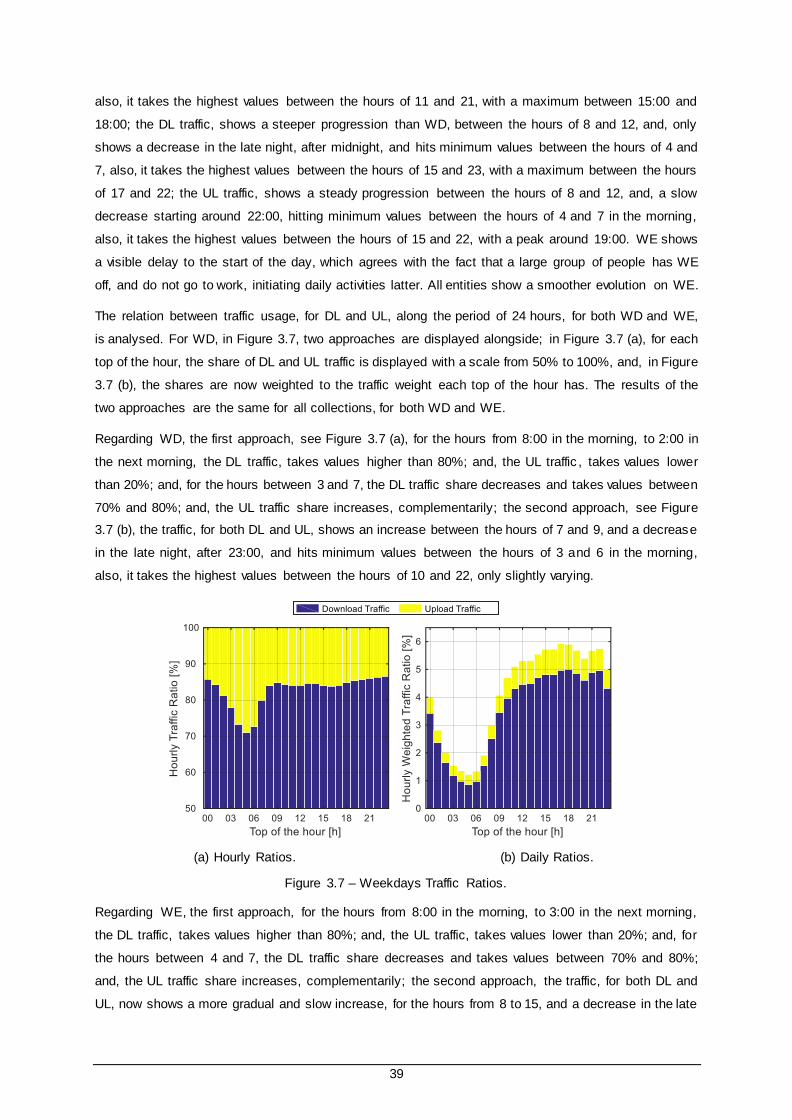
39

also, it takes the highest values between the hours of 11 and 21, with a maximum between 15:00 and

18:00; the DL traffic, shows a steeper progression than WD, between the hours of 8 and 12, and, only

shows a decrease in the late night, after midnight, and hits minimum values between the hours of 4 and

7, also, it takes the highest values between the hours of 15 and 23, with a maximum between the hours

of 17 and 22; the UL traffic, shows a steady progression between the hours of 8 and 12, and, a slow

decrease starting around 22:00, hitting minimum values between the hours of 4 and 7 in the morning,

also, it takes the highest values between the hours of 15 and 22, with a peak around 19:00. WE shows

a visible delay to the start of the day, which agrees with the fact that a large group of people has WE

off, and do not go to work, initiating daily activities latter. All entities show a smoother evolution on WE.

The relation between traffic usage, for DL and UL, along the period of 24 hours, for both WD and WE,

is analysed. For WD, in Figure 3.7, two approaches are displayed alongside; in Figure 3.7 (a), for each

top of the hour, the share of DL and UL traffic is displayed with a scale from 50% to 100%, and, in Figure

3.7 (b), the shares are now weighted to the traffic weight each top of the hour has. The results of the

two approaches are the same for all collections, for both WD and WE.

Regarding WD, the first approach, see Figure 3.7 (a), for the hours from 8:00 in the morning, to 2:00 in

the next morning, the DL traffic, takes values higher than 80%; and, the UL traffic , takes values lower

than 20%; and, for the hours between 3 and 7, the DL traffic share decreases and takes values between

70% and 80%; and, the UL traffic share increases, complementarily; the second approach, see Figure

3.7 (b), the traffic, for both DL and UL, shows an increase between the hours of 7 and 9, and a decrease

in the late night, after 23:00, and hits minimum values between the hours of 3 and 6 in the morning,

also, it takes the highest values between the hours of 10 and 22, only slightly varying.

(a) Hourly Ratios. (b) Daily Ratios.

Figure 3.7 – Weekdays Traffic Ratios.

Regarding WE, the first approach, for the hours from 8:00 in the morning, to 3:00 in the next morning,

the DL traffic, takes values higher than 80%; and, the UL traffic, takes values lower than 20%; and, for

the hours between 4 and 7, the DL traffic share decreases and takes values between 70% and 80%;

and, the UL traffic share increases, complementarily; the second approach, the traffic, for both DL and

UL, now shows a more gradual and slow increase, for the hours from 8 to 15, and a decrease in the late

40

night, after 23:00, hitting the minimum values between the hours of 4 and 7, and taking the highest

values between the hours of 15 and 23.

3.3.3 Applications Results

The distribution of each entity, through the applications, is shown for all 24 top of the hour, for both WD

and WE. Two analyses are represented, firstly, the share of entity associated to each one of the

applications is displayed, taking values between 0% and 100% for each top of the hour, see Figure 3.8

for WD; later, the shares are weighted to the entity weight each top of the hour has, and all hours have

to add up to 100%, see Figure 3.9 for WD. The first analysis helps to grasp the impact each application

has for each hour, and how it changes along the day. The second one, displays the actual contributions

each application represents in the day.

Figure 3.8 – Weekdays APP_GROUP Hourly Ratios.

Figure 3.9 – Weekdays APP_GROUP Daily Ratios.

41

Comparing WD against WE, some subtle changes are visible; in particular, applications associated with

business activities, show a reduction during WE; and, an application used all week, but showing an

increase on WE, suggests that it is often used for personal and free time. The outside contours of Figure

3.9, equal the ones seen in Figure 3.6, but now with the applications’ contribution. These visual aids

allow to gain some understanding on the behaviours evolution along the day, and give an insight to

which equations and models to use to describe and predict these behaviours. The differences between

WD and WE, for the daily ratios, were discussed for the hour weights and the App hourly ratios.

Regarding the App collection and WD, see Figure 3.10, the NU, for M2M and WebAp, takes values

higher than 15%; for E-mail, FiTr, Games, InMe, Other and Streaming, takes values between 15% and

5%; and, for P2P and VoIP, takes values lower than 5%; the DL traffic, for Streaming and WebAp, takes

values higher than 35%; for FiTr, takes a value between 15% and 5%; for M2M and P2P, takes values

between 5% and 2%; and, for E-mail, Games, InMe, Other and VoIP, takes values lower than 2%; the

UL traffic, for Streaming and WebAp, takes values higher than 20%; for FiTr, M2M, P2P and VoIP, takes

values between 15% and 5%; for E-mail and Other, takes values between 5% and 2%; and, for Games

and InMe, takes values lower than 2%. Although E-mail, Games, InMe and M2M correspond to around

53% of the NU, combined only represent 6% of DL traffic and 11% of UL traffic; in contrast, Streaming

and WebAp only correspond to around 25% of the NU, and add up to 78% of DL traffic and to 55% of

UL traffic. For WE, the NU are around the same values, and the traffic usage, for both DL and UL, vary

slightly, with the biggest change occurring for Streaming, which increases.

Figure 3.10 – Weekdays APP_GROUP Aggregated Daily Ratios.

3.3.4 Devices Results

The distribution of each entity through the devices is shown for all 24 top of the hour, for both WD and

WE. Two analysis are represented, firstly, the share of entity associated to each one of the devices is

displayed, taking values between 0% and 100% for each top of the hour, see Figure 3.11 for WD; later,

the shares are weighted to the entity weight each top of the hour has, and all hours have to add up to

100%, see Figure 3.12 for WD. The first analysis helps to grasp the influence each device has for each

hour, and how it changes along the day. The second one, displays the concrete contributions each

42

device represents in the day.

Figure 3.11 – Weekdays DEV_TYPE Hourly Ratios.

Figure 3.12 – Weekdays DEV_TYPE Daily Ratios.

Comparing WD against WE, the most visible difference is that WE have smother evolutions throughout

the day. The outside contours of Figure 3.12, equal the ones seen in Figure 3.6, but now displaying the

devices’ contributions. These visual aids allow to gain some understanding on the device preference

along the day, and give an insight to which equations and models to use to describe and predict these

behaviours. The differences between WD and WE, for the daily ratios, were discussed for the hour

weights and the Dev hourly ratios. Regarding the Dev collection and WD, see Figure 3.13, the NU, for

Smartphone, takes a value higher than 85%; for Hotspots, Others, Pens, Routers and Tablet, takes

values lower than 5%; the DL traffic, for Smartphone, takes a value higher than 40%; for Hotspots, Pens

and Routers, takes values between 25% and 10%; for Others and Tablet, takes values lower than 5%;

the UL traffic, for Routers, takes a value higher than 35%; for Hotspots and Smartphones, takes values

between 30% and 20%; for Pens, takes values between 15% and 5%; and, for Others and Tablets,

43

takes values lower than 5%. Although Smartphone corresponds to around 88% of the NU, it only

represents 42% of DL traffic and 28% of UL traffic; in contrast, Hotspots, Pens and Routers correspond

to around 7% of the NU, and add up to 53% of DL traffic and to 67% of UL traffic. For WE, the NU are

around the same values, and the traffic usage, for both DL and UL, vary slightly; Hotspots, Smartphones

and Tablets show an increase.

Figure 3.13 – Weekdays DEV_TYPE Aggregated Daily Ratios.

3.3.5 Operating Systems Results

The distribution of each entity through the operating systems is shown for all 24 top of the hour, for both

WD and WE. Two analysis are represented, firstly, the share of entity associated to each one of the

operating systems is displayed, taking values between 0% and 100% for each top of the hour, see

Figure 3.14 for WD; later, the shares are weighted to the entity weight each top of the hour has, and all

hours have to add up to 100%, see Figure 3.15 for WD. The first analysis helps to grasp the share each

operating system has for each hour, and how it changes along the day. The second one, displays the

contributions each operating system represents in the day.

Comparing WD against WE, the most visible difference is that WE have smother evolutions throughout

the day. The outside contours of Figure 3.15, equal the ones seen in Figure 3.6, but now displaying the

operating systems’ contributions. These visual aids allow to gain some understanding on the operating

systems reach along the day, and give an insight to which equations and models to use to describe and

predict these behaviours. The differences between WD and WE, for the daily ratios, were discussed for

the hour weights and the OpS hourly ratios. Regarding the OpS collection and WD, see Figure 3.16, the

NU, for Android and iOS, takes values higher than 40%; and, for Others and Windows, takes values

lower than 10%; the DL traffic, for Android and Others, takes values higher than 30%; for iOS, takes a

value between 25% and 20%; and, for Windows, takes a value lower than 2%; the UL t raffic, for Android

and Others, takes values higher than 40%; for iOS, takes a value around 15%; and, for Windows, takes

a value lower than 2%. Android and iOS add up to roughly 90% of the NU, and represent around 56%

of DL traffic and UL traffic. For WE, the NU and the traffic usage, for both DL and UL, are roughly

maintained the same.

44

Figure 3.14 – Weekdays OP_SYS Hourly Ratios.

Figure 3.15 – Weekdays OP_SYS Daily Ratios.

Figure 3.16 – Weekdays OP_SYS Aggregated Daily Ratios.

45

3.3.6 Maximum Traffic Percent Change

To have a better understanding of the traffic variations between WD and WE, for both DL and UL; and

between DL and UL, for both WD and WE, these variations are quantified with the maximum traffic

change. The maximum traffic change is used in two angles, in comparing WD against WE, and, in

comparing DL against UL. Percent changes are obtained for both DL and UL, when comparing WD

against WE; and, for both WD and WE, when comparing DL against UL; a total of four situations are

analysed. The maximum traffic change considers as the reference and observed values, the maximum

traffic 𝑇[𝐺𝐵] observed for a particular 𝑛 case of a collection. For the comparison between WD and WE,

WD is the reference value and WE is the observed one; and, for the comparison between DL and UL,

DL is the reference value and UL is the observed one. A decrease, symbolised with the minus sign,

means that the maximum DL traffic is higher than the maximum UL traffic, whereas an increase means

the opposite. Each one of these variations is presented, for each collection, and for each one of the

respective 𝑛 cases, in Table 3.6 for the App collection, in Table 3.7 for the Dev collection, and in Table

3.8 for the OpS collection.

Regarding the App collection, when comparing WD against WE, for DL, the highest percent change is

obtained for E-mail, at a decrease of 63.62%, and the lowest one is obtained for WebAp, at a decrease

of 2.02%; when comparing WD against WE, for UL, the highest percent change is obtained for E-mail,

at a decrease of 61.44%, and the lowest one is obtained for Streaming, at an increase of 1.99%. For

both DL and UL there is a percent change decrease for E-mail, FiTr, M2M, Other, VoIP and WebAp;

and a percent change increase for Games, InMe, P2P and Streaming. E-mail shows a large decrease,

from WD to WE, which is in accordance with the fact that it is mainly used in a work environment and

for labour activities. Games, InMe, P2P and Streaming show a s light increase, from WD to WE, which

suggests and supports that these are applications are for personal and free time use.

Regarding the App collection, when comparing DL against UL, for WD, the highest percent change is

obtained for Streaming, at a decrease of 91.12%, and the lowest one is obtained for VoIP, at a decrease

of 12.25%; when comparing DL against UL, for WE, the highest percent change is obtained for

Streaming, at a decrease of 91.6%, and the lowest one is obtained for VoIP, at a decrease of 8.54%.

For both WD and WE, the maximum DL traffic is always higher than the maximum UL traffic. The percent

change for DL against UL varies between a decrease of 63% and 92%, with the exceptions of InMe,

Other, P2P, and VoIP for which it varies between a decrease of 8% and 39%. VoIP can be considered

a symmetric conversational service, with a percent change for DL against UL, at a decrease of 12.25%

for WD, and at a decrease of 8.54% for WE. InMe is an interactive service often used for dialogue

purposes, which explains the low percent changes obtained. For both WD and WE, the highest percent

changes are obtained for Streaming, and the lowest ones are obtained for VoIP.

Regarding the Dev collection, when comparing WD against WE, for DL, the highest percent change is

obtained for Others, at a decrease of 32%, and the lowest one is obtained for Hotspots, at an increase

of 0.16%; when comparing WD against WE, for UL, the highest percent change is obtained for Pens, at

a decrease of 32.47%, and the lowest one is obtained for Smartphone, at a decrease of 1.78%. For both

DL and UL there is a percent change decrease for Others, Pens and Routers; and a percent change

46

increase for Hotspots and Tablet; with the exception of Smartphone that has a percent change at an

increase of 0.60% for DL, and at a decrease of 1.78% for UL. Hotspots and Smartphones , for DL, have

a percent change of nearly 0%, and for UL, have an increase of 3.25% and a decrease of 1.78%,

respectively, which suggests an overall usage independent of WD or WE. Tablet shows an usage

increase on WE, for both DL and UL, suggesting that this device is used for personal and leisure times.

Regarding the Dev collection, when comparing DL against UL, for WD, the highest percent change is

obtained for Tablet, at a decrease of 91.20%, and the lowest one is obtained for Routers, at a decrease

of 69.27%; when comparing DL against UL, for WE, the highest percent change is obtained for Tablet ,

at a decrease of 90.35%, and the lowest one is obtained for Others, at a decrease of 69.07%. For both

WD and WE, the maximum DL traffic is always higher than the maximum UL traffic. The percent change

for DL against UL varies between a decrease of 69% and 92%; and, for each one of the devices, the

obtained values for WD and WE are very similar.

Table 3.6 – APP_GROUP Traffic Percent Change.

App Collection

Maximum Traffic Change [%]

Weekdays vs Weekends Download vs Upload

Download Upload Weekdays Weekends

(1) E-Mail -63.62 -61.44 -65.29 -63.21

(2) FiTr -26.30 -25.12 -83.20 -82.94

(3) Games 23.76 9.34 -74.12 -77.14

(4) InMe 13.78 13.02 -26.63 -27.12

(5) M2M -17.15 -36.67 -67.28 -74.99

(6) Other -47.88 -27.58 -38.66 -14.77

(7) P2P 12.99 17.43 -21.94 -18.87

(8) Streaming 8.28 1.99 -91.12 -91.64

(9) VoIP -6.70 -2.76 -12.25 -8.54

(10) WebAp -2.02 -13.55 -84.83 -86.61

Table 3.7 – DEV_TYPE Traffic Percent Change.

Dev Collection




(1) Hotspots 0.16 3.25 -85.91 -85.48

(2) Others -32.00 -25.58 -71.74 -69.07

(3) Pens -9.98 -32.47 -78.24 -83.68

(4) Routers -20.68 -19.93 -69.27 -68.97

(5) Smartphone 0.60 -1.78 -87.16 -87.46

(6) Tablet 17.96 29.34 -91.20 -90.35

Regarding the OpS collection, when comparing WD against WE, for DL, the highest percent change is

obtained for iOS, at an increase of 8.90%, and the lowest one is obtained for Windows, at an increase

of 0.42%; when comparing WD against WE, for UL, the highest percent change is obtained for Windows,

at an increase of 25.31%, and the lowest one is obtained for iOS, at an increase of 1.42%. For both DL

and UL there is a percent change decrease for Android and Others; and a percent change increase for

Windows and iOS. The percent change for WD against WE varies between an increase of 0% and 26%,

and a decrease of 2 and 13%.

Regarding the OpS collection, when comparing DL against UL, for WD, the highest percent change is

47

obtained for iOS, at a decrease of 86.87%, and the lowest one is obtained for Android, at a decrease of

79.17%; when comparing DL against UL, for WE, the highest percent change is obtained for iOS, at a

decrease of 87.77%, and the lowest one is obtained for Android, at a decrease of 80.25%. For both WD

and WE, the maximum DL traffic is always higher than the maximum UL traffic. The percent change for

DL against UL varies between a decrease of 79% and 88%; and, for each one of the operating systems,

the obtained values for WD and WE are very similar. For both WD and WE, the highest percent changes

are obtained for iOS, and the lowest ones are obtained for Android.

Table 3.8 – OP_SYS Traffic Percent Change.

OpS Collection




(1) Android -7.54 -12.32 -79.17 -80.25

(2) Others -2.11 -2.65 -83.73 -83.82

(3) Windows 0.42 25.31 -85.47 -81.86

(4) iOS 8.90 1.42 -86.87 -87.77

3.4 Model Catalogue

The model catalogue contains the models used as the set of hypotheses when looking for regression

models to explain the data. The list of tested models is: Trapezoid model, Tree Stump model, Pyramid

model, Thorn model, Gaussian model, Double Gaussian model and Triple Gaussian model. Three types

of equations are chosen as the basis to all models, they are the linear equation, the exponential equation

and the gaussian equation. Each model can assemble one or more sections.

Linear equation,

𝑓𝑙𝑖𝑛 𝐾(𝑥) = 𝑚𝐾 𝑥 + 𝑏𝐾 (3.19)

where:

• 𝑚𝐾 : slope;

• 𝑏𝐾: initial value;

• 𝐾: section index.

Exponential equation,

𝑓𝑒𝑥𝑝 𝐾(𝑥) = 𝑐𝐾 + 𝑒

(𝑥−𝑡𝐾)

𝑘𝐾 (3.20)

where:

• 𝑐𝐾: vertical offset;

• 𝑡𝐾 : translation in time;

• 𝑘𝐾 : decay rate.

Gaussian equation,

𝑓𝑔𝑎𝑢𝑠𝑠 𝐾(𝑥) = 𝑣𝐾 + 𝑢𝐾 1

√2𝜋σ𝐾2𝑒

−(𝑥−μ𝐾)2

2σ𝐾2

(3.21)

where:

48

• 𝑣𝐾 : vertical offset;

• 𝑢𝐾: scaling factor;

• σ𝐾 : dispersion factor;

• μ𝐾 : average.

A visual aid for the model catalogue is presented in Figure 3.17, showing how many sections each

model has, and with which equations is built.

(a) Trapezoid. (b) Tree Stump.

(c) Pyramid. (d) Thorn Left.

(e) Thorn Right. (f) Gaussian.

(g) Double Gaussian. (h) Triple Gaussian.

Figure 3.17 – Model Fitting Options.

The initial and final points of the model, 𝑋𝑖 and 𝑋𝑓 , limit to the left the first section and to the right the last

section of the model, respectively. If the model has more than one section, the breakpoints between

sections are 𝑋1 , section limit one, and 𝑋2 , section limit two.

The Trapezoid model has three linear sections,

𝑓𝑇𝑅𝐴𝑃𝑍𝑂𝐼𝐷 (𝑥) = {

𝑓𝑙𝑖𝑛 1(𝑥), 𝑋𝑖 ≤ 𝑥 ≤ 𝑋1𝑓𝑙𝑖𝑛 2(𝑥), 𝑋1 ≤ 𝑥 ≤ 𝑋2𝑓𝑙𝑖𝑛 3(𝑥), 𝑋2 ≤ 𝑥 ≤ 𝑋𝑓

(3.22)

The Tree Stump model has three sections, two exponential sections and a linear section, between them,

𝑓𝑇𝑅𝐸𝐸 𝑆𝑇𝑈𝑀𝑃(𝑥) = {

𝑓𝑒𝑥𝑝 1(𝑥), 𝑋𝑖 ≤ 𝑥 ≤ 𝑋1𝑓𝑙𝑖𝑛 2(𝑥), 𝑋1 ≤ 𝑥 ≤ 𝑋2𝑓𝑒𝑥𝑝 3(𝑥), 𝑋2 ≤ 𝑥 ≤ 𝑋𝑓

(3.23)

The Pyramid model has two linear sections,

𝑓𝑃𝑌𝑅𝐴𝑀𝐼𝐷 (𝑥) = {𝑓𝑙𝑖𝑛 1(𝑥), 𝑋𝑖 ≤ 𝑥 ≤ 𝑋1𝑓𝑙𝑖𝑛 2(𝑥), 𝑋1 ≤ 𝑥 ≤ 𝑋𝑓

(3.24)

The Thorn Left model has two sections, an exponential followed by a linear section,

49

𝑓𝑇𝐻𝑂𝑅𝑁𝐿 (𝑥) = {𝑓𝑒𝑥𝑝 1 (𝑥), 𝑋𝑖 ≤ 𝑥 ≤ 𝑋1𝑓𝑙𝑖𝑛 2(𝑥), 𝑋1 ≤ 𝑥 ≤ 𝑋𝑓

(3.25)

The Thorn Right model has two sections, a linear followed by an exponential section,

𝑓𝑇𝐻𝑂𝑅𝑁𝑅 (𝑥) = {𝑓𝑙𝑖𝑛 1(𝑥), 𝑋𝑖 ≤ 𝑥 ≤ 𝑋1𝑓𝑒𝑥𝑝 2 (𝑥), 𝑋1 ≤ 𝑥 ≤ 𝑋𝑓

(3.26)

The Gaussian model has one gaussian section,

𝑓𝐺𝐴𝑈𝑆𝑆𝐼𝐴𝑁(𝑥) = 𝑓𝑔𝑎𝑢𝑠𝑠 (𝑥), 𝑋𝑖 ≤ 𝑥 ≤ 𝑋𝑓 (3.27)

The Double Gaussian model has two gaussian sections,

𝑓𝐷𝑂𝑈𝐵𝐿𝐸 𝐺𝐴𝑈𝑆𝑆𝐼𝐴𝑁(𝑥) = {𝑓𝑔𝑎𝑢𝑠𝑠 1(𝑥), 𝑋𝑖 ≤ 𝑥 ≤ 𝑋1𝑓𝑔𝑎𝑢𝑠𝑠 2(𝑥), 𝑋1 ≤ 𝑥 ≤ 𝑋𝑓

(3.28)

The Triple Gaussian model has three gaussian sections,

𝑓𝑇𝑅𝐼𝑃𝐿𝐸 𝐺𝐴𝑈𝑆𝑆𝐼𝐴𝑁(𝑥) = {

𝑓𝑔𝑎𝑢𝑠𝑠 1(𝑥), 𝑋𝑖 ≤ 𝑥 ≤ 𝑋1𝑓𝑔𝑎𝑢𝑠𝑠 2(𝑥), 𝑋1 ≤ 𝑥 ≤ 𝑋2𝑓𝑔𝑎𝑢𝑠𝑠 3(𝑥), 𝑋2 ≤ 𝑥 ≤ 𝑋𝑓

(3.29)

Each model is identified as follows: Trapezoid (T); Tree Stump (TS); Pyramid (P); Thorn Left (TL); Thorn

Right (TR); Gaussian (G); Double Gaussian (DG); Triple Gaussian (TG).

3.5 Implementation Methodology

The data is organised and categorised so information about each study case can be accessed. The

different collections, profiles, entities, links, and cases of each collection, add up to 120 distinct study

cases. A statistical modelling methodology is implemented in MATLAB, to obtain regression models that

characterise the study cases.

3.5.1 Data Structuring and Processing

The Data Processing, see Figure 3.19, starts with loading the raw data from the file, into a table in

MATLAB; retrieving the names of the applications, devices and operating systems ; and defining a data

structure. Profile definition, see Figure 3.21, establishes the WD and WE, and separates the date logs

between the two profiles. The data is structured as depicted in Figure 3.22. For each profile, either WD

or WE, one uses the profile indexes to identify the respective rows in the raw data table; the raw data

table entries are then loaded into the data structure. Next, for each entity, the raw data table entries are

loaded into the data structure; for each profile, the respective date logs and time logs are drew; and, for

each day, one obtains the total data for a specific hour, by combining all data entries with the same date

log and time log. The 583885 raw data entries are organised into the data structure that has 24 entries,

one for each top of the hour, and as many columns as the profile’s number of days, 26 for WD and 13

for WE. In case the original file may be missing some entry log, the data set undergoes a process that

checks for and corrects any faults detected. The implementation assumes that each day entry (column)

50

has 24 sequential hour entries (rows); the training data set file has two types of faults: 8 days are missing

one hour log, and 1 day has one data log filled under an hour log different from the top of the hour.

Knowing the value each time log must have, and the right order in which it appears, it is possible to

identify the time logs missing in the days at fault. The detected faults are corrected by applying linear

interpolation to the data set, using the interp1 command in MATLAB [50].

For the descriptive statistical analysis, one obtains the average of each hour and the average standard

deviation. The data points and the average curves undergo a time shift. The shift implementation begins

with the task of finding the global minimum of the average curve. The objective behind shifting and

rearranging the data, is making it easier to visually recognise shapes and the sections’ limits; but also,

to facilitate the fitting process. The global minimum is shifted to the left limit of the time window; the

same shift is applied to the rest of the data points, and to the average curves. Data shifting is equivalent

to performing a translation of the time logs. Histograms provide an initial understanding of the data

scatter distribution about the average; and, the lillietest MATLAB command is performed for a 5% level

of significance to assess if the data statistical distribution can be considered normal. The shifted data

and the shifted average curve are normalised to the maximum value of the average curve.

3.5.2 Fitting Process

For the Fitting Process, see Figure 3.20, the initial guess, or the starting values of the coefficients affects

the convergence of the fitting algorithm. The data is not approximated by a single function; the model is

obtained by assembling the section’s equation results. Sectioning the model creates added difficulties,

from defining the limits of each section, to guaranteeing the continuity at the breakpoints between

sections; and, since the data has a cyclic daily window, there is also the need to guarantee the continuity

between the left and right limits of the model.

The 3 equations types are defined, the model catalogue is listed, and each one of the 8 models is built

by assembling the respective sections’ equations. Each model has a different number of sections and

different types of section’s equations, which influence the number of coefficients estimated for each

model. The fit MATLAB command performs curve fitting for one fitType at a time, using a nonlinear

least-squares algorithm [51], but is unable to yield a discontinuity free model; many manually set

attempts would have to be tested, without knowing if a viable model could be found. Prevent ive

measures must be taken so only models suitable to the data, and with positive values, can be obtained.

The section’s limits, and options for the coefficients values, can be appointed from inspecting the

average curves, but is not practical to individually defined each, due to the large number of study cases

and unknows. The starting values, for initialisation, and upper and lower bounds, are established for

each one of the model’s coefficients, and breakpoints between sections. At the same time, continuity

between adjacent sections, and the initial and final points of the model, must be ensured.

One assumes the amplitude, for the left and right section limits of a 𝐾𝑡ℎ section, as 𝑌𝑙𝑒𝑓𝑡𝐾 and 𝑌𝑟𝑖𝑔ℎ𝑡

𝐾 ,

respectively. To ensure continuity for a model with only one section, one only needs to guaranty that the

initial and final amplitudes of the model, 𝑌𝑙𝑒𝑓𝑡1 and 𝑌𝑟𝑖𝑔ℎ𝑡

1 , are equal; for a model with two sections, one

51

needs to guaranty that 𝑌𝑙𝑒𝑓𝑡1 = 𝑌𝑟𝑖𝑔ℎ𝑡

2 and 𝑌𝑟𝑖𝑔ℎ𝑡1 = 𝑌𝑙𝑒𝑓𝑡

2 ; and, for a model with three sections, one needs

to guaranty that 𝑌𝑙𝑒𝑓𝑡1 = 𝑌𝑟𝑖𝑔ℎ𝑡

3 , 𝑌𝑟𝑖𝑔ℎ𝑡1 = 𝑌𝑙𝑒𝑓𝑡

2 and 𝑌𝑟𝑖𝑔ℎ𝑡2 = 𝑌𝑙𝑒𝑓𝑡

3 . To fulfil these conditions, an Auxiliary

Model 𝑓(𝑋), is introduced. Each one of the three types of equations, used as the basis to all models,

can be regarded as a variant of the auxiliary model, with an allied Auxiliary Function 𝐹(𝑋).

The Auxiliary Model,

𝑓(𝑋) = 𝑏𝑚𝑑𝑙 𝐹(𝑋) + 𝑎𝑚𝑑𝑙 (3.30)

where:

• 𝑏𝑚𝑑𝑙 : auxiliary model coefficient 1;

• 𝐹(𝑋): auxiliary function;

• 𝑎𝑚𝑑𝑙 : auxiliary model coefficient 2.

The Linear Auxiliary Function, with 𝑏𝑚𝑑𝑙 = 𝑚𝐾 and 𝑎𝑚𝑑𝑙 = 𝑏𝐾,

𝐹(𝑋) = 𝑋 (3.31)

The Exponential Auxiliary Function, with 𝑏𝑚𝑑𝑙 = 1 and 𝑎𝑚𝑑𝑙 = 𝑐𝐾 ,

𝐹(𝑋) = 𝑒(𝑋−𝑡)

𝑘 (3.32)

The Gaussian Auxiliary Function, with 𝑏𝑚𝑑𝑙 = 𝑢𝐾 and 𝑎𝑚𝑑𝑙 = 𝑣𝐾 ,

𝐹(𝑋) =1

√2𝜋σ2𝑒−(𝑋−μ)2

2σ2 (3.33)

For each section, a two-equation system is used to define the left limit, (𝑋1 , 𝑌1), and the right limit,

(𝑋2 ,𝑌2). The system’s solutions are 𝑎𝑚𝑑𝑙 and 𝑏𝑚𝑑𝑙 .

{𝑓(𝑋1 ) = 𝑌1𝑓(𝑋2 ) = 𝑌2

⇔ {𝑏𝑚𝑑𝑙 𝐹(𝑋1 ) + 𝑎𝑚𝑑𝑙 = 𝑌1𝑏𝑚𝑑𝑙 𝐹(𝑋2 ) + 𝑎𝑚𝑑𝑙 = 𝑌2

(3.34)

𝑎𝑚𝑑𝑙 =𝑌1𝐹(𝑋2 ) − 𝑌2𝐹(𝑋1)

𝐹(𝑋2) − 𝐹(𝑋1 ) (3.35)

𝑏𝑚𝑑𝑙 =𝑌2− 𝑌1

𝐹(𝑋2 ) − 𝐹(𝑋1) (3.36)

The Exponential equation sections are the exception. To obtain reasonable values for the estimations

of the coefficients, and for the width of the coefficient’s CI, one coefficient is fixed, specifically 𝑏𝑚𝑑𝑙 = 1;

the quality of the fitting adjustment is not compromised. For the exponential auxiliary function, the

system’s solutions are 𝑡𝑚𝑑𝑙 and 𝑘𝑚𝑑𝑙.

𝑡𝑚𝑑𝑙 =𝑋1 𝑙𝑜𝑔(𝑌2− 𝑎𝑚𝑑𝑙 ) − 𝑋2 𝑙𝑜𝑔(𝑌1− 𝑎𝑚𝑑𝑙 )

𝑙𝑜𝑔(𝑌1− 𝑎𝑚𝑑𝑙 ) − 𝑙𝑜𝑔(𝑌2− 𝑎𝑚𝑑𝑙 ) (3.37)

𝑘𝑚𝑑𝑙 =𝑋1 − 𝑋2

𝑙𝑜𝑔(𝑌1− 𝑎𝑚𝑑𝑙 ) − 𝑙𝑜𝑔(𝑌2− 𝑎𝑚𝑑𝑙 ) (3.38)

For the rest of the points where continuity must be ensured, the same approach applies. Depending on

what type of section equation it is, different system’s solutions are used. The expressions for 𝑎𝑚𝑑𝑙 , 𝑏𝑚𝑑𝑙 ,

𝑡𝑚𝑑𝑙 , and 𝑘𝑚𝑑𝑙 , are placed into the original models, from the model catalogue, in accordance with each

section’s equation. At the end of the fitting process, the coefficient’s values are retrieved based on the

same respective expressions.

52

For the actual fitting process, not all coefficients’ estimations , and resulting models, are suitable for the

respective study case. A method must be in place to discard unwanted results. A limit of 10 viable model

hypotheses is established, for each one of the 8 catalogue models, and from which the best hypothesis

is selected. The coefficients’ and breakpoints’ initialisation values , and upper and lower bounds, are

used to reduce the range of possibilities, when testing a hypothesis, and avoid senseless results. An

iterative condition is implemented, that establishes the coefficient’s CI width to a minimum of 1, and, if

the fit MATLAB command is unable to return an estimation, increments the width until a solution is

reached. Each time a hypothesis is obtained, its results are compared against the ones from the

previously obtained hypothesis, and the better one prevails to be compared again against the ones from

the next obtained hypothesis, until 10 have been tested.

The CD results, obtained from comparing each model hypothesis against the average curve, are used

as criteria to decide which hypothesis is better, between the two; the better option is the one with higher

CD. This process is completed when, within the stated conditions, all 8 models are obtained. For each

one of the 8 models, the GOF statistics’ results are obtained per section, from comparing the model

against data; and from comparing the model against the data’s average curve, as seen in Figure 3.18.

Start

GOF statistics

RMSE

Coefficient of Determination

Adjusted Coefficient of

Determination

Compare model against

Data

All sections checked?RMSE

Coefficient of Determination

Adjusted Coefficient of

Determination


average curve

NO

YES

End

Figure 3.18 – Goodness of fit statistics.

53

Start

Load raw data set from file

Identify cases

Create the data structure

Structure Data

Data scatter distribution

inspection

Profile definition

All data collections

checked?

All profiles checked?All data collections

checked?

All data collections

checked?

NO

YES

All profiles checked?

NO

All entities checked?

NO

YES

Continue

All cases checked?

NOYES

Descriptive statistical

analysis

Shift implementation

NO

NO

YES

NO

YES

YES

Figure 3.19 – Data Processing.

54

Normalise shifted data

Normalise shifted average

EndAll data collections

checked?

All profiles checked?

NO


NO

YES

All cases checked?

NOYES

NO

Model Catalogue

Implementation

All 8 models checked?

All 10 hypotheses

tested?

NO

Model Fittype Validation

Calculate GOF statistics


average curve

New model better than best hypothesis

model?

Best hypothesis model

equals the new model

Best hypothesis model

remains the same

YES NO

NO

Assemble model

coefficients for best

hypothesis model

YES

Continue

Save record of the 8 best

modelsYES

YES

YES

Figure 3.20 – Fitting Process.

55

StartProfile definition

Organise the date log into

workdays and weekendsEnd

Define workdays and

weekends

All days checked?

Draw the date logs

NO

YES

Figure 3.21 – Profile definition.

StartStructure DataLoad raw data set

Select raw data for entity

Draw the date logs

Draw the time logs

Combine data with the

same date log and time log

Check and correct any fault

from the raw data set

End


All cases checked?

NO

YESNO

YES

Figure 3.22 – Structure data.

3.6 Model Comparison and Ranking

3.6.1 Goodness of Fit Statistics Results

The statistics’ results are obtained from comparing the normalised shifted models with the respective

normalised shifted average curves. The goodness of fit statistics are used to evaluate the fit of the

obtained models against the respective data curves. The RMSE, the CD and the ACD are used as

criteria of comparison, and ranking, between the obtained models. The goal is to find the models that

fulfil the most number of criteria. A model fulfils each criteria if the statistics’ results are closer to the

preferable ones, than the results obtained for the other model hypothesis. For more accurate and

meaningful results, only eligible models that guaranty a RMSE lower than 10%, and a CD and an ACD

56

higher than 90% will be used to represent each data collection. A colour criteria scheme is implemented

to aid in the survey and comparison of the results, see Figure 3.23. For the RMSE, the lowest values,

starting in 0%, are coloured in green, becoming lighter until a middle point at 10%, with yellow, and then

becoming darker up to red, at an established maximum of 20%. For the CD and the ACD, the highest

values, up to 100%, are coloured in green, becoming lighter until the values lower to 80%, with yellow,

and then becoming darker up to red at an established minimum of 60%. The break points at 10% and

80%, respectively, define the value after which the results must be taken with extra caution. Values

higher than 20% for the RMSE, and values lower than 60% for both the CD and the ACD, are considered

unreliable results and are to be discarded, and the respective models are found questionable in its ability

to predict the data. Models that are good approximations for the data often have very similar values in

the range between [90,100]%; this highlights the models that are to be considered as the hypothesis for

Best and General models.

(a) RMSE √𝜀2̅̅ ̅[%].

(b) CD 𝑅2[%]; ACD 𝑅𝑎𝑑𝑗2

[%].

Figure 3.23 – Goodness of fit statistics’ colour criteria.

The combination of each of the three tables allows to compare the models, and helps rank them in

agreement with the established criteria, with the objective of finding the Best and General models. For

each case of a collection (one column of the tables), each section of the table is analysed and the

models ranked, and then the criteria decisions are combined. This procedure is repeated for each

column of the four scenarios: WD, DL; WD, UL; WE, DL; WE, UL. The criteria decisions require ordering

the models in ascendant order for the RMSE, and in descendent order for both the CD and the ACD.

For the App collection, and the scenario WD, DL, when comparing the results of the 8 models, see Table

3.9, regarding the RMSE, the lowest value is obtained for M2M and VoIP, with the TG model, at 1.9%,

and the highest one is obtained for WebAp, with the TR model, at 16.2%; regarding the CD, the highest

value is obtained for M2M and VoIP, with the TG model, at 99.6%, and the lowest one is obtained for

P2P, with the TL model, at 65.3%; and, regarding the ACD, the highest value is obtained for M2M and

VoIP, with the TG model, at 99.3%, and the lowest one is obtained for P2P, with the TL model, at 60.1%.

For the App collection, and the scenario WD, UL, when comparing the results of the 8 models, regarding

the RMSE, the lowest value is obtained for VoIP, with the TG model, at 1.7%, and the highest one is

obtained for WebAp, with the TR model, at 13.1%; regarding the CD, the highest value is obtained for

VoIP, with the TG model, at 99.6%, and the lowest one is obtained for Streaming, with the TL model, at

80.6%; and, regarding the ACD, the highest value is obtained for VoIP, with the TG model, at 99.3%,

and the lowest one is obtained for Streaming, with the TL model, at 77.7%.

For the App collection, and the scenario WE, DL, when comparing the results of the 8 models, regarding

57

the RMSE, the lowest value is obtained for InMe, with the TG model, at 1.0%, and the highest one is

obtained for Streaming, with the TL model, at 13.5%; regarding the CD, the highest value is obtained

for InMe, with the TG model, at 99.9%, and the lowest one is obtained for Streaming, with the TL model,

at 79.0%; and, regarding the ACD, the highest value is obtained for InMe, with the TG model, at 99.8%,

and the lowest one is obtained for Streaming, with the TL model, at 75.8%.

For the App collection, and the scenario WE, UL, when comparing the results of the 8 models, regarding

the RMSE, the lowest value is obtained for VoIP and WebAp, with the TS and TG models, respectively ,

at 1.4%, and the highest one is obtained for WebAp, with the TL model, at 12.5%; regarding the CD, the

highest value is obtained for WebAp, with the TG model, at 99.8%, and the lowest one is obtained for

WebAp, with the TL model, at 83.3%; and, regarding the ACD, the highest value is obtained for WebAp,

with the TG model, at 99.7%, and the lowest one is obtained for WebAp, with the TL model, at 80.7%.

Table 3.9 – Weekdays Download APP_GROUP.

(1)

E-Mail

(2)

FiTr

(3)

Games

(4)

InMe

(5)

M2M

(6)

Other

(7)

P2P

(8)

Streaming

(9)

VoIP

(10)

WebAp

RMSE √𝜀2̅̅̅ [%]

T 9.5 7.2 4.5 7.6 5.4 8.9 7.9 4.0 6.7 6.8

TS 4.1 3.5 4.2 6.0 4.2 9.8 4.3 2.5 2.8 4.4

P 10.1 13.3 5.5 11.2 10.8 10.4 12.3 8.0 8.1 14.3

TL 10.2 12.3 6.1 14.3 12.5 10.9 13.5 11.9 11.8 16.1

TR 12.3 15.9 5.9 12.7 13.3 9.7 8.6 6.4 4.1 16.2

G 10.5 13.2 6.7 9.1 10.1 11.2 9.6 10.6 11.7 12.3

DG 4.4 8.1 3.8 6.3 6.8 8.9 6.7 5.7 6.0 11.5

TG 2.9 3.2 3.0 3.0 1.9 8.4 5.5 2.1 1.9 4.3

CD 𝑅2[%]

T 92.5 94.6 97.2 95.4 96.9 87.8 88.2 98.0 94.6 95.9

TS 98.6 98.7 97.6 97.2 98.2 85.2 96.4 99.2 99.1 98.3

P 91.5 81.4 95.9 90.0 87.6 83.3 71.4 91.8 92.1 81.8

TL 91.3 84.1 94.9 83.8 83.5 81.6 65.3 81.8 83.2 77.2

TR 87.5 73.6 95.2 87.3 81.4 85.3 85.8 94.7 97.9 76.9

G 90.8 81.7 94.0 93.5 89.3 80.5 82.3 85.5 83.4 86.7

DG 98.4 93.1 98.0 96.8 95.1 87.7 91.4 95.8 95.7 88.4

TG 99.3 98.9 98.8 99.3 99.6 89.2 94.2 99.4 99.6 98.3

ACD 𝑅𝑎𝑑𝑗 2 [%]

T 90.9 93.5 96.6 94.5 96.2 85.3 85.7 97.6 93.4 95.0

TS 98.1 98.3 96.7 96.2 97.5 79.9 95.1 98.9 98.7 97.7

P 90.7 79.7 95.5 89.1 86.4 81.7 68.7 91.0 91.4 80.1

TL 90.0 81.7 94.1 81.3 81.0 78.8 60.1 79.1 80.6 73.7

TR 85.6 69.6 94.5 85.4 78.6 83.1 83.7 93.9 97.6 73.4

G 89.4 79.0 93.1 92.5 87.7 77.6 79.6 83.3 81.0 84.7

DG 97.8 90.7 97.3 95.7 93.4 83.3 88.4 94.3 94.1 84.3

TG 98.8 98.1 97.8 98.7 99.3 80.9 89.7 99.0 99.3 97.1

For the App collection, the RMSE varies between 1% and 16.2%; the CD varies between 99.9% and

65.3%; and, the ACD varies between 99.8% and 60.1%.

For WD, DL, concerning the Streaming case, going back to Table 3.9, regarding the RMSE, the lowest

values are obtained with the TG model, at 2.1%, and with the TS model, at 2.5%; regarding the CD, the

highest values are obtained with the TG model, at 99.4%, and with the TS model, at 99.2%; and,

regarding the ACD, the highest values are obtained with the TG model, at 99.0%, and with the TS model,

58

at 98.9%. A model that presents the best results for a statistic fulfils the criteria for that statistic. A model

with statistics results closer to the preferable ones for the three statistics, fulfils the three criteria the

best, and is ranked first, which is what happens with the TG model. The TS model is ranked second, as

it is the second best model to satisfies all three criteria. It is possible to guaranty a RMSE lower than

3%, a CD higher than 99%, and an ACD higher than 98%. The same procedure is repeated for the

remaining applications, for all scenarios.

For the Dev collection, and the scenario WD, DL, when comparing the results of the 8 models, regarding

the RMSE, the lowest value is obtained for Hotspots, with the TG model, at 1.9%, and the highest one

is obtained for Pens, with the TR model, at 17.5%; regarding the CD, the highest value is obtained for

Pens, with the TG model, at 99.6%, and the lowest one is obtained for Pens, with the TR model, at

70.5%; and, regarding the ACD, the highest value is obtained for Pens, with the TG model, at 99.3%,

and the lowest one is obtained for Pens, with the TR model, at 66.1%.

For the Dev collection, and the scenario WD, UL, when comparing the results of the 8 models, regarding

the RMSE, the lowest value is obtained for Routers, with the TG model, at 1.5%, and the highest one is

obtained for Tablet, with the TR model, at 15.4%; regarding the CD, the highest value is obtained for

Tablet, with the TG model, at 99.6%, and the lowest one is obtained for Others, with the G model, at

46.9%; and, regarding the ACD, the highest value is obtained for Tablet, with the TG model, at 99.3%,

and the lowest one is obtained for Others, with the G model, at 39.0%.

For the Dev collection, and the scenario WE, DL, when comparing the results of the 8 models, regarding

the RMSE, the lowest value is obtained for Hotspots, with the TS model, at 1.5%, and the highest one

is obtained for Tablet, with the TL model, at 15.8%; regarding the CD, the highest value is obtained for

Hotspots, with the TS model, at 99.7%, and the lowest one is obtained for Tablet, with the TL model, at

71.3%; and, regarding the ACD, the highest value is obtained for Hotspots, with the TS model, at 99.6%,

and the lowest one is obtained for Tablet, with the TL model, at 67.0%.

For the Dev collection, and the scenario WE, UL, when comparing the results of the 8 models, regarding

the RMSE, the lowest value is obtained for Smartphone, with the TG model, at 0.9%, and the highest

one is obtained for Others, with the TL model, at 17.1%; regarding the CD, the highest value is obtained

for Smartphone, with the TG model, at 99.9%, and the lowest one is obtained for Others, with the TL

model, at 68.5%; and, regarding the ACD, the highest value is obtained for Smartphone, with the TG

model, at 99.8%, and the lowest one is obtained for Others, with the TL model, at 63.8%.

For the Dev collection, the RMSE varies between 0.9% and 17.5%; the CD varies between 99.9% and


For WD, DL, concerning the Smartphone case, regarding the RMSE, the lowest values are obtained

with the TS model, at 5.2%, and with the T model, at 6.7%; regarding the CD, the highest values are

obtained with the TS model, at 97.2%, and with the T model, at 95.5%; and, regarding the ACD, the

highest values are obtained with the TS model, at 96.2%, and with the T model, at 94.5%. A model that

presents the best results for a statistic fulfils the criteria for that statistic. A model with statistics results

closer to the preferable ones for the three statistics, fulfils the three criteria the best, and is ranked first,

59

which is what happens with the TS model. The T model is ranked second, as it is the second best model

to satisfies all three criteria. It is possible to guaranty a RMSE lower than 7%, a CD higher than 95%,

and an ACD higher than 94%. The same procedure is repeated for the remaining devices, for all

scenarios.

For the OpS collection, and the scenario WD, DL, when comparing the results of the 8 models, regarding

the RMSE, the lowest value is obtained for Others, with the TG model, at 2.1%, and the highest one is

obtained for Windows, with the TL model, at 16.8%; regarding the CD, the highest value is obtained for

Android, with the TG model, at 99.1%, and the lowest one is obtained for Windows, with the TL model,

at 68.2%; and, regarding the ACD, the highest value is obtained for Others, with the TG model, at 99.0%,

and the lowest one is obtained for Windows, with the TL model, at 63.4%.

For the OpS collection, and the scenario WD, UL, when comparing the results of the 8 models, regarding

the RMSE, the lowest value is obtained for Others, with the TG model, at 0.9%, and the highest one is

obtained for iOS, with the TL model, at 13.7%; regarding the CD, the highest value is obtained for

Others, with the TG model, at 99.9%, and the lowest one is obtained for Others, with the TR model, at

81.4%; and, regarding the ACD, the highest value is obtained for Others, with the TG model, at 99.8%,

and the lowest one is obtained for Others, with the TR model, at 78.6%.

For the OpS collection, and the scenario WE, DL, when comparing the results of the 8 models, regarding

the RMSE, the lowest value is obtained for Others, with the TS model, at 1.5%, and the highest one is

obtained for Android, with the TL model, at 13.7%; regarding the CD, the highest value is obtained for

Others, with the TS and TG models, at 99.7%, and the lowest one is obtained for Android, with the TL

model, at 80.4%; and, regarding the ACD, the highest value is obtained for Others, with the TS model,

at 99.6%, and the lowest one is obtained for Android, with the TL model, at 77.5%.

For the OpS collection, and the scenario WE, UL, when comparing the results of the 8 models, regarding

the RMSE, the lowest value is obtained for iOS, with the TG model, at 1.0%, and the highest one is

obtained for Windows, with the TR model, at 12.1%; regarding the CD, the highest value is obtained for

iOS, with the TG model, at 99.9%, and the lowest one is obtained for Windows, with the TR model, at

81.7%; and, regarding the ACD, the highest value is obtained for iOS, with the TG model, at 99.8%, and

the lowest one is obtained for Windows, with the TR model, at 78.9%.

For the OpS collection, the RMSE varies between 0.9% and 16.8%; the CD varies between 99.9% and


For WD, DL, concerning the Android case, regarding the RMSE, the lowest values are obtained with the

TG model, at 3.1%, and with the TS model, at 4.0%; regarding the CD, the highest values are obtained

with the TG model, at 99.1%, and with the TS model, at 98.4%; and, regarding the ACD, the highest

values are obtained with the TG model, at 98.3%, and with the TS model, at 97.8%. A model that

presents the best results for a statistic fulfils the criteria for that statistic. A model with statistics results

closer to the preferable ones for the three statistics, fulfils the three criteria the best, and is ranked first,

which is what happens with the TG model. The TS model is ranked second, as it is the second best

model to satisfies all three criteria. It is possible to guaranty a RMSE lower than 4%, a CD higher than

60

98%, and an ACD higher than 97%. The same procedure is repeated for the remaining devices, for all

scenarios.

3.6.2 Best Ranked Models

The number of fulfilled criteria ranges between a maximum of three fulfilled criteria and a minimum of 1,

with a colour scale of green for three, yellow for two, and red for 1. A model that presents the best results

for a statistic fulfils the criteria for that statistic. A model that fulfils the three criteria with ranking one is

the model that best satisfies all three criteria. The following tables are the product of the inspection and

comparison of the GOF statistics tables. The focus is on the first and second ranked models. The Best

Models guaranty a √𝜀2̅̅ ̅ ≤ 10% , a 𝑅2 ≥ 95% and a 𝑅𝑎𝑑𝑗2 ≥ 90%, with a more narrow and restricted range

of results for the CD than the ones set initially.

For the App collection, and the scenario WD, DL, when ranking and attaining the number of fulfilled

criteria for the models hypothesis, see Table 3.10, the TG model is ranked as first, for 8 out of 10 cases,

and ranked as second for 2; the TS model is ranked as first for 2 cases, and ranked as second for 6;

the DG and T models are ranked as second. For 7 out of 10 cases, the first and second best models

fulfil all three criteria for having the statistics results closer to the preferable ones for the three statistics;

and for 3 cases, only two criteria are fulfilled for both.

Table 3.10 – Weekdays Download APP_GROUP Best Models.

(1)

E-Mail

(2)

FiTr

(3)

Games

(4)

InMe

(5)

M2M

(6)

Other

(7)

P2P

(8)

Streaming

(9)

VoIP

(10)

WebAp

Ranking

1º TG TG TG TG TG TG TS TG TG TS

2º TS TS DG TS TS T TG TS TS TG

Number of Fulfilled Criteria

1º 3 2 3 3 3 2 3 3 3 2

2º 3 2 3 3 3 2 3 3 3 2

For WD, DL, concerning the FiTr case, going back to Table 3.9, the TG model shows better statistic

results for the RMSE and the CD, than the TS model, with the exception of the ACD, for which the TS

model shows better results; in this way, the TG and TS models do not fulfil one of the criteria for first

and second rank, respectively, attaining both two criteria checked for their rank, see Table 3.10,

regarding the number of fulfilled criteria. Similar conditions happen for Other and WebAp.

For the App collection, and the scenario WD, UL, when ranking and attaining the number of fulfilled

criteria for the models hypothesis, the TG model is ranked as first, for 7 out of 10 cases, and ranked as

second for 1; the TS model is ranked as first for 1 case, and ranked as second for 3; the DG model is

ranked as first for 2 cases, and ranked as second for 5; the T model is ranked as second. For 9 out of

10 cases, the first and second best models fulfil all three criteria for having the statistics results closer

to the preferable ones for the three statistics; and for 1 case, only two criteria are fulfilled for both.

For the App collection, and the scenario WE, DL, when ranking and attaining the number of fulfilled


second for 3; the TS model is ranked as first for 3 cases, and ranked as second for 6; the DG model is

61

ranked as first for 1 case, and ranked as second for 1; the T model is ranked as first. For 7 out of 10

cases, the first and second best models fulfil all three criteria for having the statistics results closer to

the preferable ones for the three statistics; for 2 cases, the first fulfils all three criteria and the second

only two; and for 1 case, only two criteria are fulfilled for both.

For the App collection, and the scenario WE, UL, when ranking and attaining the number of fulfill ed


second for 1; the TS model is ranked as first for 2 cases, and ranked as second for 2; the DG model is

ranked as second for 5 cases; the T model is ranked as first for 1 case, and ranked as second for 1. For

7 out of 10 cases, the first and second best models fulfil all three criteria for having the statistics results

closer to the preferable ones for the three statistics; for 2 cases, the first fulfils all three criteria and the

second only two; and for 1 case, only two criteria are fulfilled for both.

For the Dev collection, and the scenario WD, DL, when ranking and attaining the number of fulfilled

criteria for the models hypothesis, see Table 3.11, the TG model is ranked as first, for 3 out of 6 cases,

and ranked as second for 1; the TS model is ranked as first for 3 cases, and ranked as second for 3;

the DG and T models are ranked as second. For 5 out of 6 cases, the first and second best models fulfi l

all three criteria for having the statistics results closer to the preferable ones for the three statistics; and

for 1 case, the first fulfils all three criteria and the second only two.

Table 3.11 – Weekdays Download DEV_TYPE Best Models.

(1)

Hotspots

(2)

Others

(3)

Pens

(4)

Routers

(5)

Smartphone

(6)

Tablet

Ranking

1º TG TG TG TS TS TS

2º TS TS TS DG T TG


1º 3 3 3 3 3 3

2º 3 2 3 3 3 3

For the Dev collection, and the scenario WD, UL, when ranking and attaining the number of fulfilled

criteria for the models hypothesis, the TG model is ranked as first, for all 6 cases; the TS model is ranked

as second for 4 cases; the DG model is ranked as second for 2 cases. For all 6 cases, the first and

second best models fulfil all three criteria for having the statistics results closer to the preferable ones

for the three statistics.

For the Dev collection, and the scenario WE, DL, when ranking and attaining the number of fulfilled


second for 2; the TS model is ranked as first for 3 cases, and ranked as second for 1; the DG and T

models are ranked as second. For all 6 cases, the first and second best models fulfil all three criteria for

having the statistics results closer to the preferable ones for the three statistics .

For the Dev collection, and the scenario WE, UL, when ranking and attaining the number of fulfilled


second for 2; the TS model is ranked as first for 2 cases; the DG model is ranked as second for 4 cases.

For 5 out of 6 cases, the first and second best models fulfil all three criteria for having the statistics

62

results closer to the preferable ones for the three statistics; and for 1 case, the first fulfils all three criteria

and the second only two.

For the OpS collection, and the scenario WD, DL, when ranking and attaining the number of fulfilled

criteria for the models hypothesis, see Table 3.12, the TG model is ranked as first, for 2 out of 4 cases;

the TS model is ranked as first for 2 cases, and ranked as second for 2; the T model is ranked as second.

For 9 out of 10 cases, the first and second best models fulfil all three criteria for having the statistics

results closer to the preferable ones for the three statistics; and for 1 case, only two criteria are fulfilled

for both. For all 4 cases, the first and second best models fulfil all three criteria for having the statistics

results closer to the preferable ones for the three statistics.

Table 3.12 – Weekdays Download OP_SYS Best Models: Ranking.

(1)

Android

(2)

Others

(3)

Windows

(4)

iOS

Ranking

1º TG TG TS TS

2º TS TS T T


1º 3 3 3 3

2º 3 3 3 3

For the OpS collection, and the scenario WD, UL, when ranking and attaining the number of fulfilled


as second for 1 case; the DG and T models are ranked as second. For 3 out of 4 cases, the first and

second best models fulfil all three criteria for having the statistics results closer to the preferable ones

for the three statistics; and for 1 case, only two criteria are fulfilled for both.

For the OpS collection, and the scenario WE, DL, when ranking and attaining the number of fulfilled


second for 1; the TS model is ranked as first for 1 case, and ranked as second for 3. For 3 out of 4

cases, the first and second best models fulfil all three criteria for having the statistics results closer to

the preferable ones for the three statistics; and for 1 case, the first fulfils all three criteria and the second

only two.

For the OpS collection, and the scenario WE, UL, when ranking and attaining the number of fulfilled


as second for 1 case; the DG and T models are ranked as second. For all 4 cases, the first and second

best models fulfil all three criteria for having the statistics results closer to the preferable ones for the

three statistics.

Regarding the best ranked models, for the App collection, the more used models are TG, TS and DG;

for the Dev collection, the more used models are TG, TS and DG; and, for the OpS collection, the more

used models are TG and TS.

3.6.3 General Models

For some cases, even though a model is not ranked in the best models, its statistic values are within

63

the intended and satisfactory range to obtain a reliable model. General Models guaranty a √𝜀2̅̅ ̅ ≤ 10% ,

a 𝑅2 ≥ 95% and a 𝑅𝑎𝑑𝑗2 ≥ 90% , with a more narrow and restricted range of results for the CD than the

ones set initially.

For the App collection, and the scenario WD, DL, the attributed General model, see Table 3.13 , is a TS

model for 5 out of 10 cases; is a TG model for 4 cases; is a DG model for 1 case; and is guaranteed a

√𝜀2̅̅ ̅ ≤ 4.4%, a 𝑅2 ≥ 96.4% and a 𝑅𝑎𝑑𝑗2 ≥ 95.1%, with the exception of Other, for which the best results

are √𝜀2̅̅ ̅ = 8.4%, 𝑅2 = 89.2% and 𝑅𝑎𝑑𝑗2 = 80.9%. E-mail and Games, use models that are not ranked as

first or second, but these guarantee the desired statistic values.

Table 3.13 – Weekdays Download APP_GROUP General Model.

(1)

E-Mail

(2)

FiTr

(3)

Games

(4)

InMe

(5)

M2M

(6)

Other

(7)

P2P

(8)

Streaming

(9)

VoIP

(10)

WebAp

DG TG TS TG TG TG TS TS TS TS

For the App collection, and the scenario WD, UL, the attributed General model, is a TS model for 5 out

of 10 cases; is a TG model for 4 cases; is a DG model for 1 case; and is guaranteed a √𝜀2̅̅ ̅ ≤ 5.4%, a

𝑅2 ≥ 96.3% and a 𝑅𝑎𝑑𝑗2 ≥ 94.9%. VoIP uses a model that is not ranked as first or second, but it

guarantees the desired statistic values.

For the App collection, and the scenario WE, DL, the attributed General model, is a TS model for 6 out

of 10 cases; is a TG model for 3 cases; is a P model for 1 case; and is guaranteed a √𝜀2̅̅ ̅ ≤ 4.8%, a

𝑅2 ≥ 96.2% and a 𝑅𝑎𝑑𝑗2 ≥ 95.8%. Games uses a model that is not ranked as first or second, but it

guarantees the desired statistic values.

For the App collection, and the scenario WE, UL, the attributed General model, is a TS model for 5 out

of 10 cases; is a TG model for 3 cases; is a TR model for 2 cases; and is guaranteed a √𝜀2̅̅ ̅ ≤ 5.7%, a

𝑅2 ≥ 95.3% and a 𝑅𝑎𝑑𝑗2 ≥ 93.7%. Games, M2M and P2P, use models that are not ranked as first or

second, but these guarantee the desired statistic values.

For the App collection, and General models, the RMSE varies between 1.0% and 5.7%; the CD varies

between 99.9% and 95.3%; and, the ACD varies between 99.8% and 93.7%.

For the Dev collection, and the scenario WD, DL, the attributed General model, see Table 3.14, is a TS

model for 5 out of 6 cases; is a TG model for 1 case; and is guaranteed a √𝜀2̅̅ ̅ ≤ 8.9%, a 𝑅2 ≥ 96.7%

and a 𝑅𝑎𝑑𝑗2 ≥ 95.5%.

Table 3.14 – Weekdays Download DEV_TYPE General Model.

(1)

Hotspots

(2)

Others

(3)

Pens

(4)

Routers

(5)

Smartphone

(6)

Tablet

TS TG TS TS TS TS

For the Dev collection, and the scenario WD, UL, the attributed General model, is a TS model for 5 out

of 6 cases; is a TG model for 1 case; and is guaranteed a √𝜀2̅̅ ̅ ≤ 6.4%, a 𝑅2 ≥ 95.2% and a 𝑅𝑎𝑑𝑗2 ≥

93.4%. Pens uses a model that is not ranked as first or second, but it guarantees the desired statistic

64

values.

For the Dev collection, and the scenario WE, DL, the attributed General model, is a TS model for all 6

cases; and is guaranteed a √𝜀2̅̅ ̅ ≤ 5.5%, a 𝑅2 ≥ 96.4% and a 𝑅𝑎𝑑𝑗2 ≥ 95.2%. Others and Smartphone,

use models that are not ranked as first or second, but these guarantee the desired statistic values.

For the Dev collection, and the scenario WE, UL, the attributed General model, is a TS model for all 6

cases; and is guaranteed a √𝜀2̅̅ ̅ ≤ 6.5%, a 𝑅2 ≥ 95.0% and a 𝑅𝑎𝑑𝑗2 ≥ 93.2%. Pens, Routers, Smartphone

and Tablet, use models that are not ranked as first or second, but these guarantee the desired statistic

values.

For the Dev collection, and General models, the RMSE varies between 1.5% and 8.9%; the CD varies


For the OpS collection, and the scenario WD, DL, the attributed General model, see Table 3.15, is a TS

model for all 4 cases; and is guaranteed a √𝜀2̅̅ ̅ ≤ 5.5%, a 𝑅2 ≥ 96.6% and a 𝑅𝑎𝑑𝑗2 ≥ 95.5%.

Table 3.15 – Weekdays Download OP_SYS General Model.

(1)

Android

(2)

Others

(3)

Windows

(4)

iOS

TS TS TS TS

For the OpS collection, and the scenario WD, UL, the attributed General model, is a TS model for all 4

cases; and is guaranteed a √𝜀2̅̅ ̅ ≤ 7.1%, a 𝑅2 ≥ 95.4% and a 𝑅𝑎𝑑𝑗2 ≥ 93.8%. Android, Windows and iOS

use models that are not ranked as first or second, but these guarantee the desired statistic values.

For the OpS collection, and the scenario WE, DL, the attributed General model, is a TS model for all 4

cases; and is guaranteed a √𝜀2̅̅ ̅ ≤ 4.5%, a 𝑅2 ≥ 98.0% and a 𝑅𝑎𝑑𝑗2 ≥ 97.3%.

For the OpS collection, and the scenario WE, UL, the attributed General model, is a TS model for all 4

cases; and is guaranteed a √𝜀2̅̅ ̅ ≤ 6.2%, a 𝑅2 ≥ 95.2% and a 𝑅𝑎𝑑𝑗2 ≥ 93.5%. Android, Windows and iOS

use models that are not ranked as first or second, but these guarantee the desired s tatistic values.

For the OpS collection, and General models, the RMSE varies between 1.5% and 7.1%; the CD varies


3.7 Regression Results

The entity to model is traffic usage, for both links, DL and UL, for all four scenarios: WD, DL; WD, UL;

WE, DL; WE, UL. The regression models allow to describe mathematically the data variations

throughout the day. The resulting models are used to describe the training data set, and to predict the

behaviour of new data for different input situations. The time unit is expressed in top of the hours. The

models are obtained for shifted and normalised data and average curves. The maximum value of the

65

average curve is used to normalise all results. The model, the average curve and the average standard

deviation region about the average are displayed shifted and normalised. Although the models are

obtained for the data set, the average curves provide an adequate representation of the data. Displaying

the obtained model next to the average curve gives insight to how well the model describes the

behaviour and matches the overall data observations. The average standard deviation expresses the

dispersion of data samples about the average. If the obtained model is contained by the average

standard deviation region about the average, then the regression model is more likely to provide a good

representation of the data. The final model representation is displayed for the interval between 00:00

and midnight, and is normalised to the maximum value the model may take.

The models are composed of sections characterised by linear, exponential, and gaussian equations;

each type of equation has a different set of coefficients that is estimated. The narrower the 95%

coefficients’ CIs are, the more the results can be trusted. The coefficient values are obtained for each

one of the model’s sections, with the respective CIs and GOF statistics. The GOF statistics are

presented for each one of the model’s section to better assess the fit of the model to the data, and also,

an overall assessment is obtained by comparing the model with the average curve.

The best models are the ones which fulfil the highest number of criteria for having the statistics ’ results

closer to the preferable ones. The general models are the ones that either are classified as best, or

guarantee a √𝜀2̅̅ ̅ ≤ 10% , a 𝑅2 ≥ 95% and a 𝑅𝑎𝑑𝑗2 ≥ 90% . The general models are assessed in regards

to its quality and capacity of prediction against a new data set, and scenarios.

An illustrative set of results is presented for the App, Dev and OpS collections , focusing on the general

models. Regarding the App collection, for Streaming, see Figure 3.24, a general model is presented for

each one of the four scenarios. The general models are all contained by its respective average standard

deviation region about the average; for DL traffic the region is very narrow, while for UL traffic is larger.

The average curve, in blue, is well match by all the models, in red. For WD, DL, the Streaming general

model is a TS, see Figure 3.24 (a), and has an average standard deviation lower than 6%. The first

section corresponds to the period between the hours of 6 and 10, and is associated to an exponential

equation; all coefficients show very narrow CIs, with width smaller than 1; and the GOF statistics’ results

guarantee a √𝜀2̅̅ ̅ ≤ 4.4%, a 𝑅2 ≥ 90.8% and a 𝑅𝑎𝑑𝑗2 ≥ 90.7%. The second section corresponds to the

period between the hours of 10 and 24, and is associated to a linear equation; all coefficients show very

narrow CIs, with width smaller than 2; and the GOF statistics’ results guarantee a √𝜀2̅̅ ̅ ≤ 7.2%, a 𝑅2 ≥

78.4% and a 𝑅𝑎𝑑𝑗2 ≥ 78.3%. The third section corresponds to the period between the hours of 24 and 6,

and is associated to an exponential equation; all coefficients show very narrow CIs, with width smaller

than 2; and the GOF statistics’ results guarantee a √𝜀2̅̅ ̅ ≤ 7.1%, a 𝑅2 ≥ 93.8% and a 𝑅𝑎𝑑𝑗2 ≥ 93.7%. The

comparison between the model against the average curve, guarantees a √𝜀2̅̅ ̅ ≤ 2.5%, a 𝑅2 ≥ 99.2%

and a 𝑅𝑎𝑑𝑗2 ≥ 98.9%. Having a high value for the ACD reinforces the accuracy of the CD. The final model

representation is displayed for the interval between 00:00 and midnight, and is normalised to the

maximum value the model may take. For WD and DL traffic, the Streaming final model, see Figure 3.25

(a), shows an increase in the morning, and a decrease starting around midnight, until hitting a minimum

66

at 6 in the morning, also, it takes the highest values, busy hours, between the hours of 10 and 24, where

it gradually increases.

(a) Weekdays Download plot. (b) Weekdays Upload plot.

(c) Weekends Download plot. (d) Weekends Upload plot.

Figure 3.24 – APP_GROUP Streaming General Model.



Figure 3.25 – APP_GROUP Streaming General Model 00:00 – 24:00.

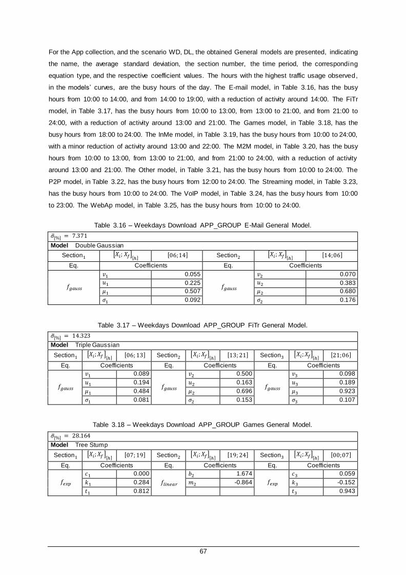
67

For the App collection, and the scenario WD, DL, the obtained General models are presented, indicating

the name, the average standard deviation, the section number, the time period, the corresponding

equation type, and the respective coefficient values. The hours with the highest traffic usage observed,

in the models’ curves, are the busy hours of the day. The E-mail model, in Table 3.16, has the busy

hours from 10:00 to 14:00, and from 14:00 to 19:00, with a reduction of activity around 14:00. The FiTr

model, in Table 3.17, has the busy hours from 10:00 to 13:00, from 13:00 to 21:00, and from 21:00 to

24:00, with a reduction of activity around 13:00 and 21:00. The Games model, in Table 3.18, has the

busy hours from 18:00 to 24:00. The InMe model, in Table 3.19, has the busy hours from 10:00 to 24:00,

with a minor reduction of activity around 13:00 and 22:00. The M2M model, in Table 3.20, has the busy

hours from 10:00 to 13:00, from 13:00 to 21:00, and from 21:00 to 24:00, with a reduction of activity

around 13:00 and 21:00. The Other model, in Table 3.21, has the busy hours from 10:00 to 24:00. The

P2P model, in Table 3.22, has the busy hours from 12:00 to 24:00. The Streaming model, in Table 3.23,

has the busy hours from 10:00 to 24:00. The VoIP model, in Table 3.24, has the busy hours from 10:00

to 23:00. The WebAp model, in Table 3.25, has the busy hours from 10:00 to 24:00.

Table 3.16 – Weekdays Download APP_GROUP E-Mail General Model.

𝜎[%] = 7.371

Model Double Gaussian

Section1 [𝑋𝑖; 𝑋𝑓][ℎ] [06;14] Section2 [𝑋𝑖; 𝑋𝑓][ℎ]

[14;06]

Eq. Coefficients Eq. Coefficients

𝑓𝑔𝑎𝑢𝑠𝑠

𝑣1 0.055


𝑣2 0.070

𝑢1 0.225 𝑢2 0.383

𝜇1 0.507 𝜇2 0.680

𝜎1 0.092 𝜎2 0.176

Table 3.17 – Weekdays Download APP_GROUP FiTr General Model.

𝜎[%] = 14.323

Model Triple Gaussian

Section1 [𝑋𝑖; 𝑋𝑓 ][ℎ] [06; 13] Section2 [𝑋𝑖; 𝑋𝑓][ℎ]

[13; 21] Section3 [𝑋𝑖; 𝑋𝑓][ℎ] [21;06]

Eq. Coefficients Eq. Coefficients Eq. Coefficients


𝑣1 0.089


𝑣2 0.500


𝑣3 0.098

𝑢1 0.194 𝑢2 0.163 𝑢3 0.189

𝜇1 0.484 𝜇2 0.696 𝜇3 0.923

𝜎1 0.081 𝜎2 0.153 𝜎3 0.107

Table 3.18 – Weekdays Download APP_GROUP Games General Model.

𝜎[%] = 28.164

Model Tree Stump


[19; 24] Section3 [𝑋𝑖; 𝑋𝑓][ℎ] [00;07]


𝑓𝑒𝑥𝑝

𝑐1 0.000

𝑓𝑙𝑖𝑛𝑒𝑎𝑟

𝑏2 1.674

𝑓𝑒𝑥𝑝

𝑐3 0.059

𝑘1 0.284 𝑚2 -0.864 𝑘3 -0.152

𝑡1 0.812 𝑡3 0.943

68

Table 3.19 – Weekdays Download APP_GROUP InMe General Model.

𝜎[%] = 9.526



[13; 22] Section3 [𝑋𝑖; 𝑋𝑓][ℎ] [22;06]



𝑣1 0.009


𝑣2 0.500


𝑣3 0.069

𝑢1 0.255 𝑢2 0.255 𝑢3 0.174

𝜇1 0.532 𝜇2 0.740 𝜇3 0.927

𝜎1 0.123 𝜎2 0.200 𝜎3 0.085

Table 3.20 – Weekdays Download APP_GROUP M2M General Model.

𝜎[%] = 9.999



[13; 21] Section3 [𝑋𝑖; 𝑋𝑓][ℎ] [21;06]



𝑣1 0.088


𝑣2 0.400


𝑣3 0.120

𝑢1 0.234 𝑢2 0.305 𝑢3 0.197

𝜇1 0.501 𝜇2 0.698 𝜇3 0.942

𝜎1 0.103 𝜎2 0.200 𝜎3 0.109

Table 3.21 – Weekdays Download APP_GROUP Other General Model.

𝜎[%] = 25.996



[14; 21] Section3 [𝑋𝑖; 𝑋𝑓][ℎ] [21;07]



𝑣1 0.037


𝑣2 0.429


𝑣3 0.110

𝑢1 0.213 𝑢2 0.100 𝑢3 0.115

𝜇1 0.551 𝜇2 0.677 𝜇3 0.916

𝜎1 0.122 𝜎2 0.115 𝜎3 0.108

Table 3.22 – Weekdays Download APP_GROUP P2P General Model.

𝜎[%] = 23.651

Model Tree Stump


[12; 24] Section3 [𝑋𝑖; 𝑋𝑓][ℎ] [00;09]


𝑓𝑒𝑥𝑝

𝑐1 0.196


𝑏2 0.472

𝑓𝑒𝑥𝑝

𝑐3 0.312

𝑘1 0.083 𝑚2 0.490 𝑘3 -0.079

𝑡1 0.550 𝑡3 0.977

Table 3.23 – Weekdays Download APP_GROUP Streaming General Model.

𝜎[%] = 5.763

Model Tree Stump


[10; 24] Section3 [𝑋𝑖; 𝑋𝑓][ℎ] [00;06]


𝑓𝑒𝑥𝑝

𝑐1 0.035


𝑏2 0.162

𝑓𝑒𝑥𝑝

𝑐3 0.000

𝑘1 0.104 𝑚2 0.879 𝑘3 -0.125

𝑡1 0.498 𝑡3 0.993

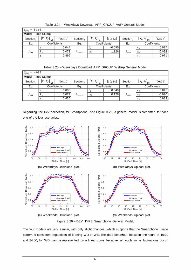
69

Table 3.24 – Weekdays Download APP_GROUP VoIP General Model.

𝜎[%] = 8.366

Model Tree Stump


[10; 23] Section3 [𝑋𝑖; 𝑋𝑓][ℎ] [23;06]


𝑓𝑒𝑥𝑝

𝑐1 0.044


𝑏2 -0.095

𝑓𝑒𝑥𝑝

𝑐3 0.027

𝑘1 0.072 𝑚2 1.126 𝑘3 -0.092

𝑡1 0.499 𝑡3 0.971

Table 3.25 – Weekdays Download APP_GROUP WebAp General Model.

𝜎[%] = 4.992

Model Tree Stump


[10; 24] Section3 [𝑋𝑖; 𝑋𝑓][ℎ] [00;06]


𝑓𝑒𝑥𝑝

𝑐1 0.000


𝑏2 0.849

𝑓𝑒𝑥𝑝

𝑐3 0.045

𝑘1 0.079 𝑚2 0.128 𝑘3 -0.090

𝑡1 0.436 𝑡3 0.983

Regarding the Dev collection, for Smartphone, see Figure 3.26, a general model is presented for each

one of the four scenarios.



Figure 3.26 – DEV_TYPE Smartphone General Model.

The four models are very similar, with only slight changes, which supports that the Smartphone usage

pattern is consistent regardless of it being WD or WE. The data behaviour between the hours of 10:00

and 24:00, for WD, can be represented by a linear curve because, although some fluctuations occur,

70

they can be considered not significant, when compared against the variation between the minimum and

maximum values. The right and left sections of the model are mostly contained by a narrow standard

deviation region, which reinforces the precision of the model.

For the Dev collection, and the scenario WD, DL, the obtained General model for the Smartphone case

is presented, indicating the name, the average standard deviation, the section number, the time period,

the corresponding equation type, and the respective coefficient values, in Table 3.26, and has the busy

hours from 09:00 to 24:00. The Dev models have the busy hours from around 10:00 to 24:00.



Figure 3.27 – DEV_TYPE Smartphone General Model 00:00 – 24:00.

Table 3.26 – Weekdays Download DEV_TYPE Smartphone General Model.

𝜎[%] = 5.585

Model Tree Stump


[09; 24] Section3 [𝑋𝑖; 𝑋𝑓][ℎ] [00;06]


𝑓𝑒𝑥𝑝

𝑐1 0.000


𝑏2 0.681

𝑓𝑒𝑥𝑝

𝑐3 0.000

𝑘1 0.058 𝑚2 0.289 𝑘3 -0.105

𝑡1 0.402 𝑡3 0.978

Regarding the OpS collection, for Android, see Figure 3.28, a General model is presented for each one

of the four scenarios. The data behaviour between the hours of 10:00 and 24:00, for DL, shows almost

no fluctuations, which support a stable usage pattern for the busy hours of the day.

71



Figure 3.28 – OP_SYS Android General Model.



Figure 3.29 – OP_SYS Android General Model 00:00 – 24:00.

72

For the OpS collection, and the scenario WD, DL, the obtained general model for the Android case is

presented, indicating the name, the average standard deviation, the section number, the time period,

the corresponding equation type, and the respective coefficient values, in Table 3.27. The OpS models

have the busy hours from 10:00 to 24:00.

Table 3.27 – Weekdays Download OP_SYS Android General Model.

𝜎[%] = 5.439

Model Tree Stump


[10; 24] Section3 [𝑋𝑖; 𝑋𝑓][ℎ] [00;06]


𝑓𝑒𝑥𝑝

𝑐1 0.000


𝑏2 0.770

𝑓𝑒𝑥𝑝

𝑐3 0.045

𝑘1 0.085 𝑚2 0.188 𝑘3 -0.097

𝑡1 0.445 𝑡3 0.971

During the development and implementation stages, one took precaution measures to safeguard the

quality of the results and guarantee a good implementation. The data statistical distribution was tested

with the goodness of fit Lilliefors test to assess if it has a normal distribution. The regression results were

compared against the data for each section, and the average curve of the data sets. The employment

of GOF statistics provides criteria to compare and rank the regression models. The visual aids

complement the statistics’ results and allow for an easy, accessible, and compact way of scrolling

through the information and checking for glitches. The Best and General models guarantee a

√𝜀2̅̅ ̅ ≤ 10% , a 𝑅2 ≥ 95% and a 𝑅𝑎𝑑𝑗2 ≥ 90%.

The next stage is to test the results against a new data set. Testing the fitting of the obtained regression

models with a new validation data set, and checking the goodness of fit statistics’ results , allow to

determine if the regression models are good at approximating the validation data set. The previous ly

obtained goodness of fit statistics’ results , when evaluating the models against the training set, are taken

as a reference, when checking the fit between those same models and the new validation set. The App

collection’s Other represents less than a 10% share of the NU, and, less than a 1% share of DL traffic;

and, the Dev collection’s Others represents less than a 2% share of the NU, and, less than a 2% share

of DL traffic; these cases are not assessed for the validation data set.

For testing the prediction quality of the regression models, one verifies if the Average Global Traffic

curve of the validation set matches well with the Prediction Global Traffic curve, based on the information

of the validation set, and the application of the regression models obtained for the training set. The

models of the App collection’s Other and Dev collection’s Others can be used since they have minimal

influence on the curve shape, given that these cases do not have a significant share of the NU, and the

traffic they generate is negligible.

73

Chapter 4

Results Analysis

4 Results Analysis

This chapter includes the models’ assessment and the traffic usage analysis for the obtained models.

The impact daily life and peoples’ routines have on network resources is presented for applications,

devices and operating systems. Recommendations and considerations are addressed for network

optimisation and efficient resource usage.

74

4.1 Models’ Assessment and Applicability

4.1.1 Validation Data Set

The new input data set, to function as validation set, was collected at the core level of the Vodafone

Portugal network, in Portugal, Lisbon, and contains 468074 observations. The observation period, from

2016/09/11 to 2016/10/12, includes 32 days, in which 22 are weekdays, 10 are weekend days, and 1 is

a national holiday day. National holiday days are considered as weekend days. For the Lisbon area, the

length of day diminishes from 2016/03/12 to 2016/04/19, going from 12h33m of daytime, to 11h17m.

The input spreadsheet file is organised into the same 8 fields as the training set.

Table 4.1 – Length of day for September and October, for the Lisbon area.

Date Sunrise Sunset Length of day

2016/09/11 07:15 19:49 12h33min

2016/10/01 07:33 19:17 11h44min

2016/10/12 07:44 19:01 11h17 min

To test the fitting of the obtained regression models with a new validation data set, one uses the same

statistics as previously, the RMSE, the CD, and the ACD. The statistics’ results obtained when

evaluating the models against the training set are taken as a reference, when checking the fit between

those same models and the new validation set. The normalised validation data is compared against the

normalised models obtained for the original training data. The outcomes, for both the General model

and the first ranked Best model are verified. Analysing the table results, the combination of each of the

three rows concerning each of the models, and the previously established criteria, allows to assess the

applicability of the models for the validation data set, and helps to evaluate their prediction capacity for

a new data set and a different time of the year. For each case of a collection, the assessment

conclusions take into consideration the results of each of the three statistics and its comparison against

the preferable values. The models are eligible, and the results reliable, if it is guaranteed that the RMSE

is lower than 15%, and the CD and the ACD are higher than 80%. With some reservations, results up

to 20% for the RMSE, and down to 70% for the CD and the ACD, are still acceptable and guarantee

reliable results. For the last two statistics, if the value goes lower than around 60%, the model must be

considered inadequate. These target values will guarantee that the models, obtained for the training

data set, are suitable to approximate and represent new information. The testing process compares the

normalised regression models against the normalised average curves of the validation data set, for a

24 top of the hour period, and is executed for all four scenarios: WD, DL; WD, UL; WE, DL; WE, UL.

For the App collection, and the scenario WD, DL, and General model results, see Table 4.2, assessing

each of the statistics results, regarding the RMSE, the lowest value is obtained for VoIP at 2.0%, and

the highest one is obtained for Games at 6.4%, with the exceptions of FiTr and P2P at around 12%;

regarding the CD, the highest value is obtained for VoIP at 99.6%, and the lowest one is obtained for

Games at 94.4%, with the exceptions of FiTr and P2P at 83.4% and 78.6%, respectively; and, regarding

the ACD, the highest value is obtained for VoIP at 99.2%, and the lowest one is obtained for Games at

90.4%, with the exceptions of FiTr and P2P at around 71.5%. When comparing the General and Best

75

models’ results against each other, no noteworthy difference is detected between the obtained values.

The General and Best models guaranteed a √𝜀2̅̅ ̅ < 7%, a 𝑅2 > 94% and a 𝑅𝑎𝑑𝑗2 > 90. FiTr and P2P

results are the ones which show the worst values, and depart the most from the preferable ones, even

so, it is guaranteed a √𝜀2̅̅ ̅ < 12%, a 𝑅2 > 78% and a 𝑅𝑎𝑑𝑗2 > 71%, signifying that predictions obtained

with these models are still reliable. The best overall statistics’ results achieved for VoIP validation data,

are highly similar to the ones obtained with the training data, and support the regularity and little

fluctuation to the behaviour of voice applications for different times of the year.

Table 4.2 – Weekdays Download APP_GROUP.

(1)

E-Mail (2) FiTr

(3) Games

(4) InMe

(5) M2M

(7) P2P

(8) Streaming

(9) VoIP

(10) WebAp

Ge

ne

ral

Mo

de

l √𝜀2̅̅̅ 5.9 11.7 6.4 5.3 4.8 11.8 4.8 2.0 5.3

𝑅2 96.6 83.4 94.4 97.8 97.5 78.6 97.0 99.6 97.6

𝑅𝑎𝑑𝑗2 94.2 71.5 90.4 96.3 95.8 71.4 94.8 99.2 96.8

Be

st

Mo

de

l √𝜀2̅̅̅ 6.6 11.7 5.9 5.3 4.8 11.8 4.5 3.0 5.3

𝑅2 95.8 83.4 95.2 97.8 97.5 78.6 97.3 99.0 97.6

𝑅𝑎𝑑𝑗2 94.4 71.5 93.6 96.3 95.8 71.4 96.4 98.7 96.8

For the App collection, and the scenario WD, UL, and General model results, assessing each of the

statistics results, the RMSE varies between 4.3% and 8.4%, with the exception of Streaming at around

21%; the CD, varies between 98.2% and 91.3%, with the exception of Streaming at around 35%; and,

the ACD, varies between 97.2% and 87.6%, with the exception of Streaming at around 13%. When

comparing the General and Best models’ results against each other, no noteworthy difference is

detected between the obtained values. The General and Best models guaranteed a √𝜀2̅̅ ̅ < 9%, a 𝑅2 >

90% and a 𝑅𝑎𝑑𝑗2 > 87%. The predictions obtained with these models are reliable.

For the App collection, and the scenario WE, DL, and General model results, assessing each of the

statistics results, the RMSE varies between 3.5% and 7.2%, with the exceptions of FiTr, P2P and VoIP,

varying between 9.2% and 11.1%; the CD, varies between 99.0% and 80.3%; and, the ACD, varies

between 98.2% and 84.6%, with the exceptions of Games at 76.4%. When comparing the General and

Best models’ results against each other, no noteworthy difference is detected between the obtained

values. The General and Best models guaranteed a √𝜀2̅̅ ̅ < 12% , a 𝑅2 > 80% and a 𝑅𝑎𝑑𝑗2 > 84%. The

predictions obtained with these models are reliable.

For the App collection, and the scenario WE, UL, and General model results, assessing each of the

statistics results, the RMSE varies between 4.8% and 6.6%, with the exceptions of Games, M2M and

P2P, varying between 9.2% and 11.0%, and Streaming at around 19%; the CD, varies between 97.6%

and 83.6%, with the exception of Streaming at around 56%; and, the ACD, varies between 95.9% and

80.7%, with the exceptions of M2M and Streaming, at 71.9% and 41.2%, respectively. When comparing

the General and Best models’ results against each other, no noteworthy difference is detected between

the obtained values. The General and Best models guaranteed a √𝜀2̅̅ ̅ < 12% , a 𝑅2 > 83% and a 𝑅𝑎𝑑𝑗2 >

80% .The predictions obtained with these models are reliable.

76

The Streaming results for UL, for both WD and WE, indicate that the model obtained for the training

data set is inadequate to characterise this particular validation data set. A closer inspection to the

Streaming curves for the validation data set, shows that the top of the hours associated to the highest

traffic usage are unchanged, when compared against the ones observed for the training data set; only

the behaviours in the early morning and in the late night differ. Streaming for UL represents a small

contribution to the overall traffic usage when compared against the DL contribution, which makes these

models’ impact negligible in the overall network resources.

Regarding the App collection, for the validation set, the General and Best models guaranteed a √𝜀2̅̅ ̅ <

12% , a 𝑅2 > 80% and a 𝑅𝑎𝑑𝑗2 > 80%; and the exception cases guaranty reliable results.

For the Dev collection, and the scenario WD, DL, and General model results, assessing each of the

statistics results, the RMSE varies between 3.6% and 6.6%; the CD, varies between 98.0% and 95.6%;

and, the ACD, varies between 96.6% and 92.8%. When comparing the General and Best models’ results

against each other, no noteworthy difference is detected between the obtained values. The General and

Best models guaranteed a √𝜀2̅̅ ̅ < 7%, a 𝑅2 > 95% and a 𝑅𝑎𝑑𝑗2 > 92%. The predictions obtained with

these models are reliable.

For the Dev collection, and the scenario WD, UL, and General model results, assessing each of the

statistics results, the RMSE varies between 4.3% and 5.9%, with the exception of Routers at 12%; the

CD, varies between 98.0% and 95.7%, with the exception of Routers at 82%; and, the ACD, varies

between 96.6% and 92.6%, with the exception of Routers at 69%. When comparing the General and

Best models’ results against each other, no noteworthy difference is detected between the obtained

values. The General and Best models guaranteed a √𝜀2̅̅ ̅ < 6%, a 𝑅2 > 95% and a 𝑅𝑎𝑑𝑗2 > 92% . Routers

results are the ones showing the worst values. The predictions obtained with these models are reliable.

For the Dev collection, and the scenario WE, DL, and General model results, assessing each of the






For the Dev collection, and the scenario WE, UL, and General model results, assessing each of the




Best models guaranteed a √𝜀2̅̅ ̅ < 14% , a 𝑅2 > 76% and a 𝑅𝑎𝑑𝑗2 > 59%. The results indicate that some

of the models must be used with caution when characterising the validation data set used. A closer

inspection to the Pens, Routers and Tablet curves, for the validation data set, show wide average

standard deviation regions about the average, and its average curves have many fluctuations, in

contrast to the ones observed for the training data set which present smoother curves despite, also,

77

having wide average standard deviation regions about the average. The predictions obtained with these

models are still reliable, even though some reservations are advised. UL traffic represents a small

contribution to the overall traffic usage when compared against the DL contribution, which makes these

models’ impact negligible in the overall network resources.

Regarding the Dev collection, for the validation set, the General and Best models guaranteed a √𝜀2̅̅ ̅ <

7%, a 𝑅2 > 94% and a 𝑅𝑎𝑑𝑗2 > 92%; and for the exception cases the results should be used with some

reservations.

For the OpS collection, and the scenario WD, DL, and General model results, assessing each of the






For the OpS collection, and the scenario WD, UL, and General model results, assessing each of the




Best models guaranteed a √𝜀2̅̅ ̅ < 11% , a 𝑅2 > 87% and a 𝑅𝑎𝑑𝑗2 > 81%. The predictions obtained with


For the OpS collection, and the scenario WE, DL, and General model results, assessing each of the






For the OpS collection, and the scenario WE, UL, and General model results, assessing each of the


and, the ACD, varies between 98.0% and 83.2%, with the exception of Android at around 71.6%. When

comparing the General and Best models’ results against each other, no noteworthy difference is

detected between the obtained values. The General and Best models guaranteed a √𝜀2̅̅ ̅ < 12% , a 𝑅2 >

83% and a 𝑅𝑎𝑑𝑗2 > 71%. The predictions obtained with these models are reliable.

Regarding the OpS collection, for the validation set, the General and Best models guaranteed a √𝜀2̅̅ ̅ <

12% , a 𝑅2 > 83% and a 𝑅𝑎𝑑𝑗2 > 71%.

For all three collections, the obtained values, for the General and Best models’ results, do not show a

mentionable difference, supporting the right decision of, in some cases, using another model as the

General model instead of the first ranked Best model. To demonstrate the ability of these models to

78

characterise and predict applications and devices behaviours, and reinforce the reliability of the results,

the average global traffic for the validation data set is approximated with the obtained models, using the

ratio inputs collected from that same validation data set.

4.1.2 Global Traffic Model

The Global Traffic Model combines all the traffic contributions related to a collection, for DL or UL, to

obtain the representation of the traffic usage for an average day from 00:00 to 24:00. For the App

collection, the traffic contribution of one application is obtained by weighing the respective General

model to its NU weight and to the maximum traffic observed for that particular application. The NU

weight, for each 𝑛 case, is provided by the Average Aggregated Daily Ratios, which give the average

contributions each case has in the duration of one day; for Streaming it is represented as 𝑤𝑛=8𝑁𝑢̅̅ ̅̅ ̅̅ ̅

. There

can be applications with the NU weight equal to 0, nonetheless, all weights must add up to 1. The

maximum traffic value is measured in Bytes, and is visually the highest peak of the regression model;

for Streaming it is represented as 𝑇𝑛=8. The regression models used are the normalised General

models, and each represents an average day from 00:00 to 24:00. These models have been normalised

to its maximum values. Regarding a data collection, the Global Traffic model, for DL or UL, is,

𝑇𝐺(𝑡) =∑𝑤𝑛𝑁𝑢̅̅ ̅̅ ̅̅ 𝑇𝑛 𝑓𝑛(𝑡)

𝑁𝑛

𝑛=1

(4.1)

where:

• 𝑓𝑛(𝑡): regression model.

The Global Traffic model can be used for approximating the average global traffic curve of a data

collection, using the NU weights and the maximum traffic values observed for that data, and leads to

the expected Global Traffic for those inputs; or can also be used for predicting the Global Traffic for

established scenarios, with defined NU weights and maximum traffic values, which is useful for studying

and understanding the impact the variation of these inputs can have on the resulting Global Traffic curve.

These two applications are implemented for the App and Dev collections. Since Android and iOS have

similar behaviours, the Global Traffic will not be addressed for the OpS collection.

4.1.2.1 Prediction Global Traffic

To test the prediction capacity of the regression models previously obtained for the training data set, the

expected Global Traffic curve, obtained using the NU weights and the maximum traffic values observed

for the validation data set, is compared against the average global traffic curve of the validation data. If

the expected outcome matches well the real average global traffic curve of the validation data, then the

regression models can predict new data sets and have a broad reach of possibilities.

The average Global Traffic curve of the validation data, either for DL or UL traffic, is obtained by adding

up all normalised average curves related to a collection, and acts as the observed global traffic curve.

The same 10 applications and 6 devices, as the ones for which the regression models were obtained,

are considered. The expected global traffic curve is obtained with the Global Traffic model, using the

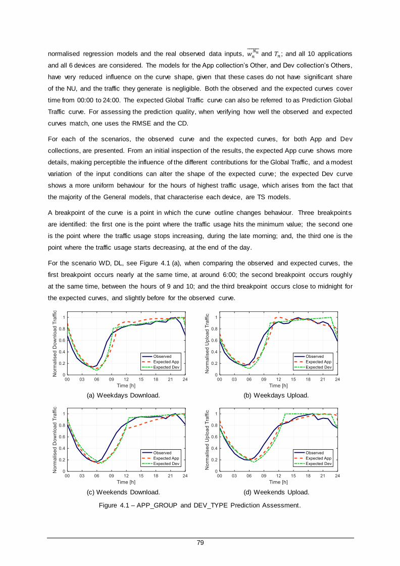
79

normalised regression models and the real observed data inputs, 𝑤𝑛𝑁𝑢̅̅ ̅̅ ̅̅

and 𝑇𝑛 ; and all 10 applications

and all 6 devices are considered. The models for the App collection’s Other, and Dev collection’s Others,

have very reduced influence on the curve shape, given that these cases do not have significant share

of the NU, and the traffic they generate is negligible. Both the observed and the expected curves cover

time from 00:00 to 24:00. The expected Global Traffic curve can also be referred to as Prediction Global

Traffic curve. For assessing the prediction quality, when verifying how well the observed and expected

curves match, one uses the RMSE and the CD.

For each of the scenarios, the observed curve and the expected curves, for both App and Dev

collections, are presented. From an initial inspection of the results, the expected App curve shows more

details, making perceptible the influence of the different contributions for the Global Traffic, and a modest

variation of the input conditions can alter the shape of the expected curve; the expected Dev curve

shows a more uniform behaviour for the hours of highest traffic usage, which arises from the fact that

the majority of the General models, that characterise each device, are TS models.

A breakpoint of the curve is a point in which the curve outline changes behaviour. Three breakpoints

are identified: the first one is the point where the traffic usage hits the minimum value; the second one

is the point where the traffic usage stops increasing, during the late morning; and, the third one is the

point where the traffic usage starts decreasing, at the end of the day.

For the scenario WD, DL, see Figure 4.1 (a), when comparing the observed and expected curves, the

first breakpoint occurs nearly at the same time, at around 6:00; the second breakpoint occurs roughly

at the same time, between the hours of 9 and 10; and the third breakpoint occurs close to midnight for

the expected curves, and slightly before for the observed curve.


(c) Weekends Download. (d) Weekends Upload.

Figure 4.1 – APP_GROUP and DEV_TYPE Prediction Assessment.

80

The statistics’ results of comparing each of the expected curves, with the observed curve, are gathered

in Table 4.3, for the App collection, and in Table 4.4, for the Dev collection. A prediction’s global traffic

is reliable if the RMSE is lower than 15%, and the CD is higher than 80%. Regarding the App collection,

the expected global traffic curves guarantee a √𝜀2̅̅ ̅ < 12% and a 𝑅2 > 84% ; and, regarding the Dev

collection, the expected global traffic curves guarantee a √𝜀2̅̅ ̅ < 11% and a 𝑅2 > 86% .

Table 4.3 – APP_GROUP Prediction Assessment.

Scenarios GOF [%] Scenarios GOF [%]

We

ekd

ays

DL √𝜀2̅̅̅ 11.64

We

eke

nd

s

DL √𝜀2̅̅̅ 10.81

𝑅2 84.10 𝑅2 86.50

UL √𝜀2̅̅̅ 8.65

UL √𝜀2̅̅̅ 8.69

𝑅2 91.62 𝑅2 90.21

Table 4.4 – DEV_TYPE Prediction Assessment.

Scenarios GOF [%] Scenarios GOF [%]

We

ekd

ays

DL √𝜀2̅̅̅ 8.79

We

eke

nd

s

DL √𝜀2̅̅̅ 10.64

𝑅2 90.91 𝑅2 86.92

UL √𝜀2̅̅̅ 8.62

UL √𝜀2̅̅̅ 9.83

𝑅2 91.65 𝑅2 87.49

When comparing the expected curves statistics’ results for the two collections against each other, for

each one of the scenarios, there is no noteworthy difference between the obtained values. Since the

statistics’ target values are satisfied, the Global Traffic Model returns reliable predictions , and the

regression models, that characterise each application or device, are suitable approximations of the

behaviours they represent, regardless of the time of the year and origin of the data set.

Although both data sets where collected for the Lisbon area, the length of day increases throughout the

days, for the training set, while decreasing for the validation set. The daytime can influence peoples ’

activity levels, motivation, disposition, and overall health. During WD, people follow a more structured

schedule, so the curves are very similar. During WE, some differences can be noted; for the training

set, as there is sunlight until later in the day, people stay active until later hours of the night; while, for

the validation set, people start the day slightly earlier to seize the natural light, and end up being less

active during the later hours of the night.

4.1.2.2 Vodafone Scenarios Prediction Global Traffic

A total of three scenarios were proposed, by Vodafone, to check the influence of the obtained models

and the prediction Global Traffic Model, in order to assess the implications different scenarios have in

the Prediction Global Traffic curve, which are helpful in evaluating the impact a scenario would have in

the network resources demands and infrastructures, throughout the day. Concerning the Global Traffic

Model, one will refer to 𝑤𝑛𝑁𝑢̅̅ ̅̅ ̅̅ 𝑇𝑛 as the scale factor of a model. Concerning the results representation,

each global traffic curve has been normalised to its maximum value.

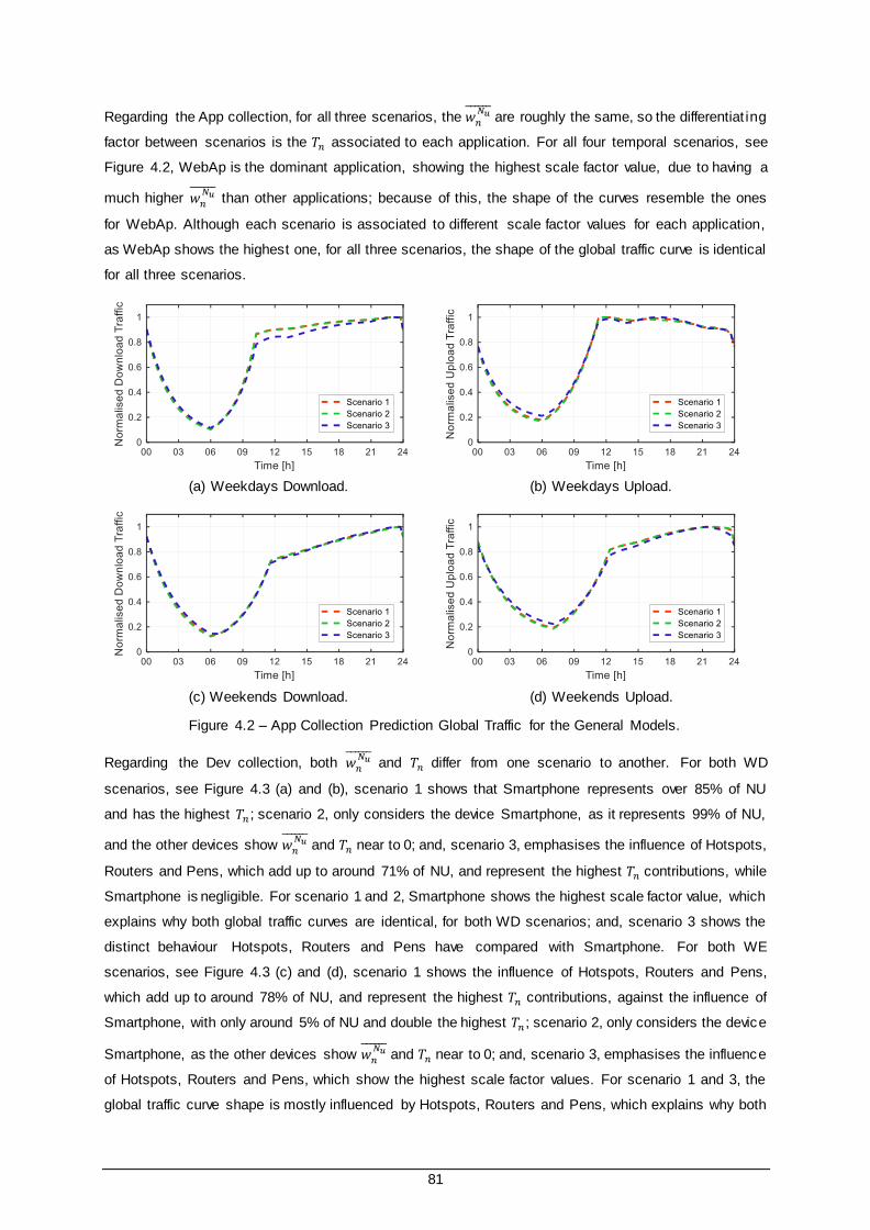
81

Regarding the App collection, for all three scenarios, the 𝑤𝑛𝑁𝑢̅̅ ̅̅ ̅̅ are roughly the same, so the differentiat ing

factor between scenarios is the 𝑇𝑛 associated to each application. For all four temporal scenarios, see

Figure 4.2, WebAp is the dominant application, showing the highest scale factor value, due to having a

much higher 𝑤𝑛𝑁𝑢̅̅ ̅̅ ̅̅ than other applications; because of this, the shape of the curves resemble the ones

for WebAp. Although each scenario is associated to different scale factor values for each application,

as WebAp shows the highest one, for all three scenarios, the shape of the global traffic curve is identical

for all three scenarios.



Figure 4.2 – App Collection Prediction Global Traffic for the General Models.

Regarding the Dev collection, both 𝑤𝑛𝑁𝑢̅̅ ̅̅ ̅̅ and 𝑇𝑛 differ from one scenario to another. For both WD

scenarios, see Figure 4.3 (a) and (b), scenario 1 shows that Smartphone represents over 85% of NU

and has the highest 𝑇𝑛 ; scenario 2, only considers the device Smartphone, as it represents 99% of NU,

and the other devices show 𝑤𝑛𝑁𝑢̅̅ ̅̅ ̅̅ and 𝑇𝑛 near to 0; and, scenario 3, emphasises the influence of Hotspots,

Routers and Pens, which add up to around 71% of NU, and represent the highest 𝑇𝑛 contributions, while

Smartphone is negligible. For scenario 1 and 2, Smartphone shows the highest scale factor value, which

explains why both global traffic curves are identical, for both WD scenarios; and, scenario 3 shows the

distinct behaviour Hotspots, Routers and Pens have compared with Smartphone. For both WE

scenarios, see Figure 4.3 (c) and (d), scenario 1 shows the influence of Hotspots, Routers and Pens,

which add up to around 78% of NU, and represent the highest 𝑇𝑛 contributions, against the influence of

Smartphone, with only around 5% of NU and double the highest 𝑇𝑛 ; scenario 2, only considers the device

Smartphone, as the other devices show 𝑤𝑛𝑁𝑢̅̅ ̅̅ ̅̅ and 𝑇𝑛 near to 0; and, scenario 3, emphasises the influence

of Hotspots, Routers and Pens, which show the highest scale factor values. For scenario 1 and 3, the

global traffic curve shape is mostly influenced by Hotspots, Routers and Pens, which explains why both

82

global traffic curves are similar, for both WE scenarios; and, scenario 2 shows the Smartphone

behaviour. The proposed scenarios allow to illustrate the prediction Global Traffic Model applicability.



Figure 4.3 – Dev Collection Prediction Global Traffic for the General Models.

4.2 Model Collections

4.2.1 Applications Models

A wide range of services and applications is offered for different operating systems , and on various

devices. The App collection data shows a broad diversity of behaviours, with a variety of peaks and

downs of activity. The obtained models, for all four scenarios, see Figure 4.4, characterise the mobile

network traffic usage for the App collection.

A visual inspection of the models’ curves show that some applications are more sensitive to daily life.

The outline of the curves exhibit two sudden traffic reductions during the busy hours, one about the

lunch time, and another, about dinner time. Lunch time varies, depending on if it is WD or WE; starting

earlier on WD, around 13:00, from the hours of 12 to 14; and, on WE, around 15:00, from the hours of

13 to 16. Dinner time is the same, for both WD and WE, from 20 to 22, with a minimum around 21. The

curves also suggest that, on WD, the day starts earlier, between 7 and 10; while on WE, starts later and

slower, from 9 to 12, which can also explain the difference between lunch hours. For both WD and WE,

the bulk of activity decreases after 22:00, with a faster reduction after midnight. During the WE,

entertainment, leisure and personal purpose applications, either maintain the same overall traffic usage

83

or show an increase in activity, since it is when most people take time to rest and pursue their interests

and hobbies.



Figure 4.4 – App Collection General Models.

Regarding the App collection, VoIP, InMe and P2P reveal symmetric traffic usage, with nearly the same

usage of DL and UL; and, E-mail, FiTr, Games, M2M, Streaming and WebAp reveal higher usage of DL

than UL.

E-mail, a background service, nowadays, is mostly used for work and business purposes; on WD, DL

traffic usage doubles the UL one, with an activity increase early in the morning and busy hours from

10:00 to 19:00; on WE, although it is used along the entire day, the overall traffic usage decreases by

half. During meal times, there is a reduction of activity.

VoIP, used for real time conversational communication between users, has DL and UL traffic usage

nearly symmetric, with busy hours from 10:00 to 23:00, while more active at the end of the day; and,

WD and WE have very similar overall traffic usage.

InMe send short messages, exchanged between users, and are often used for dialogue purposes, what

is evident from the fact that DL and UL traffic usage are nearly symmetric, with busy hours from 10:00

to 24:00, and clear decrease in activity during meal time; and, from WD to WE, the overall traffic usage

remains the same, which highlights the widespread of this group of applications, and the personal and

interactive nature of these communications.

For Games, an interactive service, the user sends signalling, to provide the game status and the play

moves thought the UL link, while the DL link is used to receive game updates, scenario changes and

84

other players moves; DL traffic usage is much higher than the UL one, with busy hours from 10:00 to

24:00, while showing more activity at the end of the day. On WE, as the number of active users

increases, so does the overall traffic usage.

P2P is used to facilitate the sharing or distribution of content and files, and the user does both the

download and then upload of the information, but also, for sending background signalling and control

messages, and continues to occur even in the early hours of the day. DL and UL traffic usage are nearly

symmetric, with busy hours from around 12:00 to 24:00; and, WD and WE overall traffic usage are

similar, with a slight increase on WE.

FiTr is used to transfer or storage files, from one location to another, and may include cloud storage and

other services. DL traffic is more than five times higher than the UL traffic, with busy hours from around

10:00 to 24:00, and a visible reduction of activity during meal times; and, from WD to WE, the overall

traffic usage only slightly decreases.

M2M can include smart meters, surveillance, alarms, terminal transactions, health, and fitness trackers,

which represent a variety of behaviours, and a large share of active users, but correspond to a very low

overall traffic usage share. During the early hours of the day, due to some of these applications, an

exchange of background signalling and status messages is maintained. DL traffic is about two times

higher than UL traffic, with busy hours from around 10:00 to 24:00, with a visible reduction of activity

during meal times, which shows the impact daily life has in some applications, included in this group,

for monitoring and tracking people’s habits ; and, on WD and WE, the overall traffic usages are similar.

WebAp and Streaming have a quarter share of the active users, and add up to almost 80% of DL traffic,

and more than half of UL traffic, making them the most influential and impactful applications when

managing and planning the network resources; and the busy hours are from around 10:00 to 24:00, for

WD, and from around 12:00 to 24:00, on WE. WebAp, an interactive service, can be personalised to the

user, and vary with each person’s likes and interest. DL traffic is more than six times higher than UL

traffic; and, from WD to WE, the overall traffic usage does not vary, which also emphasises the impact

this group of applications generates. Streaming allows for real time broadcast of audio and video, which

requires large amounts of data. DL traffic is about ten times higher than UL traffic; throughout the day,

traffic activity shows a stable rise; and, on WE, the overall traffic usage increases.

4.2.2 Devices Models

Nowadays, it is available an ample selection of devices, with different characteristics, sizes, screen

resolutions, and weights; and, the users expect to be able to access and enjoy their applications

everywhere and in the most comfortable manner. The obtained models , for all four scenarios, see Figure

4.5, characterise the mobile network traffic usage for the Dev collection. A visual inspection of the

models’ curves reveals that after midnight, up until 7:00, the traffic activity experiences a fast decrease,

which is in agreement with rest and sleep time during the night.

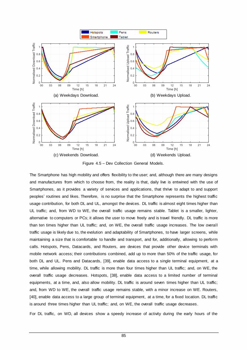
85



Figure 4.5 – Dev Collection General Models.

The Smartphone has high mobility and offers flexibility to the user; and, although there are many designs

and manufactures from which to choose from, the reality is that, daily live is entwined with the use of

Smartphones, as it provides a variety of services and applications, that thrive to adapt to and support

peoples’ routines and likes. Therefore, is no surprise that the Smartphone represents the highest traffic

usage contribution, for both DL and UL, amongst the devices. DL traffic is almost eight times higher than

UL traffic; and, from WD to WE, the overall traffic usage remains stable. Tablet is a smaller, lighter,

alternative to computers or PCs; it allows the user to move freely and is travel friendly. DL traffic is more

than ten times higher than UL traffic; and, on WE, the overall traffic usage increases. The low overall

traffic usage is likely due to, the evolution and adaptability of Smartphones, to have larger screens, while

maintaining a size that is comfortable to handle and transport, and for, additionally, allowing to perform

calls. Hotspots, Pens, Datacards, and Routers, are devices that provide other device terminals with

mobile network access; their contributions combined, add up to more than 50% of the traffic usage, for

both DL and UL. Pens and Datacards, [39], enable data access to a single terminal equipment, at a

time, while allowing mobility. DL traffic is more than four times higher than UL traffic; and, on WE, the

overall traffic usage decreases. Hotspots, [38], enable data access to a limited number of terminal

equipments, at a time, and, also allow mobility. DL traffic is around seven times higher than UL traffic;

and, from WD to WE, the overall traffic usage remains stable, with a minor increase on WE. Routers,

[40], enable data access to a large group of terminal equipment, at a time, for a fixed location. DL traffic

is around three times higher than UL traffic; and, on WE, the overall traffic usage decreases.

For DL traffic, on WD, all devices show a speedy increase of activity during the early hours of the

86

morning. Smartphone and Tablet stabilise the earliest, after 9:00; and, during commute times, due to

mobility and their compact size, allow the user, to check their e-mail, news, SNS, or read a book, in a

quick and simple manner. These types of terminals gather all conveniences in one equipment, and are

gradually replacing the paper format. Hotspots, Pens, and Routers stabilise after 10:00. On WE, all

devices stabilise later in the morning; and, the devices that experience an increase of the overall traffic

usage allow for mobility, Hotspots, Smartphone and Tablet, which can be related with the increase of

outdoors and entertainment activities. Independently of it being WD or WE, only at the end of the day,

is there a reduction of activity. For UL traffic, some curves maintain activity during the night, which

indicate the exchange of signalling and control messages, nevertheless, it represents a small

contribution to the overall traffic usage when compared against the DL contribution.

4.2.3 Operating Systems Models

Android and iOS operating systems add up to roughly 90% of the active users, and represent more than

half of the overall traffic usage. Currently, Android or iOS operating systems are mostly used in

smartphones, which is confirmed from comparing the traffic usage associated to both operating systems,

with the values observed for Smartphone, and concluding they are very similar. The obtained models,

for all four scenarios, see Figure 4.6, enlighten the resemblance, and difference, between Android and

iOS traffic usage contributions. An initial inspection to the models’ curves reveals identical focal points

and alike outline shapes. Android systems generate higher overall traffic than the iOS ones; and, during

the lower activity period, after midnight until early morning, due to background signalling, and system

and keep-alive messages, Android maintains higher UL traffic. For Android, DL traffic is around five

times higher than UL traffic; and, for iOS, DL traffic is more than seven times higher than UL traffic. The

overall traffic usage of these operating systems remains nearly the same for the entire week, which

emphasises the uniform and permanent, every day, utilisation of smartphones.


87


Figure 4.6 – OpS Collection Android and iOS General Models.

For the scenario WD, DL, see Figure 4.6 (a), both curves display nearly the same breakpoints: the

minimum value, at 6:00, and the right and left limits of the busy hours section, from around 10:00 to

24:00. These two models show similar outline shape, which emphasises that people have a global

activity pattern, regardless of the operating system that is used. The regression models, for DL traffic,

are nearly the same, especially for WD, which reveals the existence of a clear and reliable pattern, for

representing DL traffic, generated by both operating systems. The biggest differences are observed for

UL traffic, which has low impact on the overall network resources.

4.2.4 Considerations and Recommendations

Although the regression models where obtained for data collected at the core level of the Vodafone

network, for the Lisbon area, daily life and peoples’ routines can be considered global and extendable

for other regions, and for any time of the year. Combining and cross checking information and results

from the three collections, one can determine the global busy hours, as the hours from 10:00 to 24:00

for WD; and keep some reservations regarding WE, which normally present a delayed and slower start

to the days’ activities. The daytime can influence peoples’ activity levels and dispositions , which can

alter slightly the busy hours. Knowing the busy hour traffic usage allows to define the maximum traffic

capacity the network should guarantee to satisfy all active users. After midnight, up until the early hours

of the morning, there is a low activity period, that represent less than 10% of the average daily traffic

usage, and so, the available resources and, network managing structures, may be reduced, while still

maintaining QoS. To assure QoS for all data applications, different constraints must be imposed to

guarantee the different requirements of each service class. Each service class is associated to a level

of priority, from conversional, with the highest one; to streaming; to interactive; and, with the lowest

priority, background. The obtained regression models can be used to guide and establish target

resource values and help define the allocation of data rates, based on the applications inc luded in each

service class. If the objective is to know the evolution of traffic usage for a specific application, using a

real observed network measure, for a determined hour, allows to scale the model curve for the present

reality; and, the models can also be adapted to predict traffic usage for special events and different

seasons, by scaling the curves to the maximum expected values. Taking advantage of network

virtualisation and centralised managing, different network configurations may be deployed to maintain

communications, and increase efficient resource usage, for different periods of the day, with different

88

requirements. A better management of infrastructures and resources, based on the model prediction of

the behaviour of data, reduces the operators ’ costs. Users want to be able to access a vast range of

information, instantaneously, and anywhere. Portable devices gain emphasis as a daily life essential

and are replacing the paper format, like books, magazines and planners. Devices and operating systems

must be developed with the easiness of use in mind. Applications’ and devices’ activities, and operating

systems preferences, can be used to create custom and user oriented communication planes, but also

predict suitable changes to the management of network resources to accommodate the alterations of

data usage.

Understanding and being able to model data behaviours and traffic usage is crucial to the design and

optimisation of networks, as more and more content is available every day, and users play an important

role, as creators and consumers of data.

89

Chapter 5

Conclusions

5 Conclusions

This chapter summarises the development, implementation, and results of the work done, and contains

recommendations and suggestions for the applicability of the accomplished work.

90

Chapter 1 establishes the framework of the thesis and presents an overview on the current mobile

communications scenario. The motivations are addressed, the problem definition is presented, and the

structure for the thesis is provided. Chapter 2 provides a background on the fundamental concepts of

UMTS and LTE networks, detailing the architectures and radio interfaces. The quality of service is

addressed for both UMTS and LTE. Service classes and popular applications are briefly mentioned. The

characterisation of traffic models is discussed. The state of the art gathers the research that motivates

the exploratory data analysis and the development of models. Chapter 3 comprises the development

framework and the implementation description, used in the exploratory analysis of the number of active

users and traffic usage, and to obtain the models for the statistical characterisation of traffic usage, from

a live cellular network. The data is structured and analysed. The models are compared and ranked

based on goodness of fit statistics’ criteria. The regression results are found at the end. Chapter 4

includes the models’ assessment and the traffic usage analysis for the obtained models. The impact

daily life and peoples’ routines have on network resources is presented for applications, devices and

operating systems. Recommendations and considerations are addressed for network optimisation and

efficient resource usage. Chapter 5 summarises the development, implementation, and results of the

work done, and contains recommendations and suggestions for the applicability of the accomplished

work.

A data set, collected from a mobile network, can be divided between a training set and a validation set,

if the number of observations is large enough. The training set is used in the fitting process to find

prediction models; and, the validation set is used to validate the fitted models, with an independent set

of observations.

Studying and gaining a broader understanding of how impactful people’s daily lives are in application

utilisation, device preferences, and network resource demands, is relevant for network optimisation. The

purpose of this work is to characterise and represent the observed data, by providing visual aids and

mathematical models, thus highlighting patterns and better realising the implicit behaviours associated

to the distinct entities, profiles, and collections.

The applications, devices and operating systems collections are analysed, a descriptive statistical

analysis is employed, and the data statistical distribution is assessed to check if the data samples have

a normal distribution. The weighted average of the percentages of non-rejected decisions is superior to

74%, for the App collection; to 77%, for the Dev collection; and, to 76%, for the OpS collect ion. The

exploratory data analysis makes use of graphical and numerical results for an accessible and compact

representation of the data; the entities in analysis are the number of active users and traffic usage.

Although E-mail, Games, InMe and M2M correspond to around 53% of the users, combined only

represent 6% of DL traffic and 11% of UL traffic; in contrast, Streaming and WebAp only correspond to

around 25% of the users, and add up to 78% of DL traffic and to 55% of UL traffic. Although Smartphone

corresponds to around 88% of the NU, it only represents 42% of DL traffic and 28% of UL traffic; in

contrast, Hotspots, Pens and Routers correspond to around 7% of the NU, and add up to 53% of DL

traffic and to 67% of UL traffic. Android and iOS add up to roughly 90% of the users, and represent

around 56% of DL traffic and UL traffic.

91

The fitting process is implemented in MATLAB using a statistical modelling methodology, and for each

study case, provides 8 regression models, that can assemble one or more sections, with linear,

exponential, or gaussian equations, while ensuring continuity between the sections, and the initial and

final points, of the model. The obtained regression models are compared against the observed data,

and the goodness of fit statistics’ results allow for the comparison and ranking of the models, so that the

models that best approximated the data are selected.

For the App collection, the RMSE varies between 1% and 16.2%; the CD varies between 99.9% and

65.3%; and, the ACD varies between 99.8% and 60.1%. For the Dev collection, the RMSE varies

between 0.9% and 17.5%; the CD varies between 99.9% and 46.9%; and, the ACD varies between

99.8% and 39.0%. For the OpS collection, the RMSE varies between 0.9% and 16.8%; the CD varies


Regarding the best ranked models, for the App collection, the more used models are TG, TS and DG;

for the Dev collection, the more used models are TG, TS and DG; and, for the OpS collection, the more

used models are TG and TS.

For the App collection, and General models, the RMSE varies between 1.0% and 5.7%; the CD varies

between 99.9% and 95.3%; and, the ACD varies between 99.8% and 93.7%. For the Dev collection,

and General models, the RMSE varies between 1.5% and 8.9%; the CD varies between 99.7% and

95.0%; and, the ACD varies between 99.6% and 93.2%. For the OpS collection, and General models,

the RMSE varies between 1.5% and 7.1%; the CD varies between 99.7% and 95.2%; and, the ACD

varies between 99.6% and 93.5%.

The Best Models and General Models guarantee a √𝜀2̅̅ ̅ ≤ 10% , a 𝑅2 ≥ 95% and a 𝑅𝑎𝑑𝑗2 ≥ 90%.

A new data set is introduced, to assess the reliability and prediction capacity of the regression models.

The General models are compared against the validation data set; and one verifies if the Average Global

Traffic curve of the validation set, matches well with the Prediction Global Traffic curve, based on the

information of the validation set, and the application of the General models obtained for the training set.

Regarding the App collection, for the validation set, the General and Best models guaranteed a √𝜀2̅̅ ̅ <

12% , a 𝑅2 > 80% and a 𝑅𝑎𝑑𝑗2 > 80%; and the exception cases guaranty reliable results. Regarding the

Dev collection, for the validation set, the General and Best models guaranteed a √𝜀2̅̅ ̅ < 7%, a 𝑅2 > 94%

and a 𝑅𝑎𝑑𝑗2 > 92%; and for the exception cases the results should be used with some reservations.

Regarding the OpS collection, for the validation set, the General and Best models guaranteed a √𝜀2̅̅ ̅ <

12% , a 𝑅2 > 83% and a 𝑅𝑎𝑑𝑗2 > 71%.

For all three collections, the obtained values, for the General and Best models’ results, do not show a

mentionable difference, supporting the right decision of, in some cases, using another model as the

General model instead of the first ranked best model. To demonstrate the ability of these models to

characterise and predict applications and devices behaviours, and reinforce the reliability of the results,

the average global traffic for the validation data set is approximated with the obtained models, using the

ratio inputs collected from that same validation data set. The Global Traffic model can be used for

92

approximating the average global traffic curve of a data collection, and leads to the Expected Global

Traffic for that data inputs; or can also be used for predicting the Global Traffic for established scenarios,

which is useful for studying and understanding the impact the variation to the number of active users ,

and the maximum traffic values, can have on the resulting Global Traffic curve.

For the Expected Global Traffic, the expected App curve shows more details, making perceptible the

influence of the different contributions for the global traffic; the expected Dev curve shows a more

uniform behaviour for the hours of highest traffic usage, which arises from the fact that the majority of

the General models, that characterise each device, are TS models. Regarding the App collection, the

expected global traffic curves guarantee a √𝜀2̅̅ ̅ < 12% and a 𝑅2 > 84% ; and, regarding the Dev

collection, the expected global traffic curves guarantee a √𝜀2̅̅ ̅ < 11% and a 𝑅2 > 86% . The Global Traffic

Model, based on the regression models obtained, returns reliable predictions, regardless of the time of

the year and origin of the data set.

For two distinct times of the year, in which one of the periods shows the length of day increasing

throughout the days, and the other shows the length of day decreasing, for WD, people follow a more

structured schedule, so there are no noteworthy differences; for WE, as for the first case there is sunlight

until later in the day, people stay active until later hours of the night, while, for the second case, people

start the day slightly earlier to seize the natural light and end up being less active during the later hours

of the night.

For the Prediction Global Traffic curves, different scale factors, lead to different behaviours and curve

shapes, emphasising the more influential cases.

Regarding the App collection, VoIP, InMe and P2P reveal symmetric traffic usage, with nearly the same

usage of DL and UL; and, E-mail, FiTr, Games, M2M, Streaming and WebAp reveal higher usage of DL

than UL. Some applications are more sensitive to daily life. Lunch time varies depending on if it is WD

or WE; starting earlier on WD, around 13:00, from the hours of 12 to 14; and, on WE, around 15:00,

from the hours of 13 to 16. Dinner time is the same, for both WD and WE, from 20 to 22, with a minimum

around 21. For both WD and WE, the bulk of activity decreases after 22, with a faster reduction after

midnight. During the WE, entertainment, leisure and personal purpose applications, either maintain the

same overall traffic usage or show an increase in activity.

Smartphone and Tablet, during commute times, due to mobility and their compact size, allow the user,

to check their e-mail, news, SNS, or read a book, in a quick and simple manner. These types of terminals

gather all conveniences in one equipment, and are gradually replacing the paper format. Android or iOS

operating systems are mostly used in smartphones; during the lower activity period, due to background

signalling, and keep-alive messages, Android maintains higher UL traffic. The overall traffic usage of

these operating systems remains nearly the same for the entire week, which emphasises the uniform

and permanent, every day, utilisation of smartphones. Devices and operating systems must be

developed with the easiness of use in mind.

The global busy hours, for WD, are between 10:00 and 24:00; WE present a delayed and slower start

to the days’ activities. The daytime can influence peoples’ activity levels and dispositions , which can

93

alter slightly the busy hours. Knowing the busy hour traffic usage allows to define the maximum traffic

capacity the network should guarantee to satisfy all active users. After midnight, up until the early hours

of the morning, there is a low activity period, that represent less than 10% of the average daily traffic

usage, and so, the available resources and, network managing s tructures, may be reduced, while still

maintaining QoS.

For different periods of the day, with different requirements, different network configurations may be

deployed to maintain communications, and increase efficient resource usage. A better management of

infrastructures and resources, based on the model prediction of the behaviour of data, reduces the

operators’ costs.

The regression models can be used to guide and establish target resource values and help define the

allocation of data rates; or predict traffic usage by scaling the curves to the maximum expected values;

or, by combining different models, obtain a global traffic prediction. Understanding and being able to

model data behaviours and traffic usage is crucial to the design and optimisation of networks.

The regression models, either Best or General, can be tested against new data from a live cellular

network, for different regions, with different locality granularity, for different times of the year, or even

different countries, to assess if their applicability still prevails.

95

Annex A

Regression Models with

Training Data

A. Regression Models with Training Data

This Annex contains the goodness of fit statistics’ results, the Best and General regression models for

traffic usage for applications, devices, and operating systems, for both weekdays and weekends.

96

Table A.1 – APP_GROUP Best Models: Ranking.

(1)

E-Mail (2) FiTr

(3) Games

(4) InMe

(5) M2M

(6) Other

(7) P2P

(8) Streaming

(9) VoIP

(10) WebAp

WD

D

L 1º TG TG TG TG TG TG TS TG TG TS

2º TS TS DG TS TS T TG TS TS TG

WD

U

L 1º DG TG TG TG TG TG DG TS TG TG

2º TG DG TS DG DG DG TS T DG TS

WE

D

L 1º TG TG T TG TG TS DG TS TS TG

2º DG TS TS TS TS TG TS TG TG TS

WE

U

L 1º TG TG TG TG TG TG T TS TS TG

2º DG DG DG DG DG TS TG T TR TS

Table A.2 – APP_GROUP General Model.

(1)

E-Mail (2) FiTr

(3) Games

(4) InMe

(5) M2M

(6) Other

(7) P2P

(8) Streaming

(9) VoIP

(10) WebAp

WD DL DG TG TS TG TG TG TS TS TS TS

WD UL DG TG TS TG TG TG TS TS TS TS

WE DL TG TG P TG TS TS TS TS TS TS

WE UL TG TG TS TG TS TS TR TS TR TS

Table A.3 – Weekdays Download APP_GROUP E-Mail General Model.

𝜎[%] = 7.371

Model Double Gaussian

Section𝐾 [𝑋𝑖; 𝑋𝑓 ][ℎ] Eq. Coefficients

95% confidence bounds

GOF [%]

1 [06; 14] 𝑓𝑔𝑎𝑢𝑠𝑠

𝑣1 0.055 0.011 0.100 √𝜺𝟐̅̅ ̅ 11.1

𝑢1 0.225 0.196 0.254 𝑹𝟐 92.1

𝜇1 0.507 0.500 0.514 𝑹𝒂𝒅𝒋𝟐 92.0

𝜎1 0.092 0.083 0.101

2 [14; 06] 𝑓𝑔𝑎𝑢𝑠𝑠

𝑣2 0.070 0.051 0.089 √𝜺𝟐̅̅ ̅ 8.6

𝑢2 0.383 0.359 0.407 𝑹𝟐 93.7

𝜇2 0.680 0.673 0.688 𝑹𝒂𝒅𝒋𝟐 93.7

𝜎2 0.176 0.166 0.185

Model vs. Average

√𝜺𝟐̅̅ ̅ 4.4

𝑹𝟐 98.4

𝑹𝒂𝒅𝒋𝟐 97.8

97

Table A.4 – Weekdays Download APP_GROUP FiTr Best/General Model.

𝜎[%] = 14.323




GOF [%]

1 [06; 13] 𝑓𝑔𝑎𝑢𝑠𝑠

𝑣1 0.089 0.021 0.157 √𝜺𝟐̅̅ ̅ 18.3

𝑢1 0.194 0.162 0.227 𝑹𝟐 79.5

𝜇1 0.484 0.477 0.491 𝑹𝒂𝒅𝒋𝟐 79.2

𝜎1 0.081 0.071 0.092

2 [13; 21] 𝑓𝑔𝑎𝑢𝑠𝑠

𝑣2 0.500 -3.301 4.301 √𝜺𝟐̅̅ ̅ 18.5

𝑢2 0.163 -2.159 2.484 𝑹𝟐 6.6

𝜇2 0.696 0.671 0.721 𝑹𝒂𝒅𝒋𝟐 5.0

𝜎2 0.153 -0.670 0.976

3 [21; 06] 𝑓𝑔𝑎𝑢𝑠𝑠

𝑣3 0.098 0.062 0.134 √𝜺𝟐̅̅ ̅ 11.8

𝑢3 0.189 0.161 0.217 𝑹𝟐 83.9

𝜇3 0.923 0.913 0.933 𝑹𝒂𝒅𝒋𝟐 83.7

𝜎3 0.107 0.094 0.119

Model vs. Average

√𝜺𝟐̅̅ ̅ 3.2

𝑹𝟐 98.9


Table A.5 – Weekdays Download APP_GROUP Games General Model.

𝜎[%] = 28.164

Model Tree Stump



GOF [%]

1 [07; 19] 𝑓𝑒𝑥𝑝

𝑐1 0.000 -0.220 0.220 √𝜺𝟐̅̅ ̅ 25.1

𝑘1 0.284 0.141 0.427 𝑹𝟐 47.4

𝑡1 0.812 0.761 0.863 𝑹𝒂𝒅𝒋𝟐 47.1

2 [19; 24] 𝑓𝑙𝑖𝑛𝑒𝑎𝑟

𝑏2 1.674 0.208 3.139 √𝜺𝟐̅̅ ̅ 39.1

𝑚2 -0.864 -2.498 0.770 𝑹𝟐 1.1


3 [24; 07] 𝑓𝑒𝑥𝑝

𝑐3 0.059 -0.233 0.352 √𝜺𝟐̅̅ ̅ 32.5

𝑘3 -0.152 -0.297 -0.007 𝑹𝟐 28.1

𝑡3 0.943 0.907 0.979 𝑹𝒂𝒅𝒋𝟐 27.4

Model vs. Average

√𝜺𝟐̅̅ ̅ 4.2

𝑹𝟐 97.6


98

Table A.6 – Weekdays Download APP_GROUP InMe Best/General Model.

𝜎[%] = 9.526




GOF [%]

1 [06; 13] 𝑓𝑔𝑎𝑢𝑠𝑠

𝑣1 0.009 -0.054 0.072 √𝜺𝟐̅̅ ̅ 8.5

𝑢1 0.255 0.195 0.315 𝑹𝟐 92.4

𝜇1 0.532 0.515 0.548 𝑹𝒂𝒅𝒋𝟐 92.3

𝜎1 0.123 0.104 0.143

2 [13; 22] 𝑓𝑔𝑎𝑢𝑠𝑠

𝑣2 0.500 -5.693 6.693 √𝜺𝟐̅̅ ̅ 18.6

𝑢2 0.255 -4.619 5.129 𝑹𝟐 -1.9

𝜇2 0.740 0.713 0.767 𝑹𝒂𝒅𝒋𝟐 -3.4

𝜎2 0.200 -1.200 1.600

3 [22; 06] 𝑓𝑔𝑎𝑢𝑠𝑠

𝑣3 0.069 0.051 0.087 √𝜺𝟐̅̅ ̅ 7.4

𝑢3 0.174 0.155 0.193 𝑹𝟐 94.9

𝜇3 0.927 0.919 0.936 𝑹𝒂𝒅𝒋𝟐 94.8

𝜎3 0.085 0.078 0.093

Model vs. Average

√𝜺𝟐̅̅ ̅ 3.0

𝑹𝟐 99.3


Table A.7 – Weekdays Download APP_GROUP M2M Best/General Model.

𝜎[%] = 9.999




GOF [%]

1 [06; 13] 𝑓𝑔𝑎𝑢𝑠𝑠

𝑣1 0.088 0.028 0.147 √𝜺𝟐̅̅ ̅ 10.8

𝑢1 0.234 0.195 0.273 𝑹𝟐 90.4

𝜇1 0.501 0.493 0.509 𝑹𝒂𝒅𝒋𝟐 90.3

𝜎1 0.103 0.091 0.115

2 [13; 21] 𝑓𝑔𝑎𝑢𝑠𝑠

𝑣2 0.400 -1.931 2.732 √𝜺𝟐̅̅ ̅ 11.8

𝑢2 0.305 -1.547 2.157 𝑹𝟐 22.6

𝜇2 0.698 0.682 0.715 𝑹𝒂𝒅𝒋𝟐 21.4

𝜎2 0.200 -0.254 0.654

3 [21; 06] 𝑓𝑔𝑎𝑢𝑠𝑠

𝑣3 0.120 0.085 0.156 √𝜺𝟐̅̅ ̅ 9.4

𝑢3 0.197 0.164 0.230 𝑹𝟐 89.2

𝜇3 0.942 0.929 0.954 𝑹𝒂𝒅𝒋𝟐 89.1

𝜎3 0.109 0.095 0.123

Model vs. Average

√𝜺𝟐̅̅ ̅ 1.9

𝑹𝟐 99.6


99

Table A.8 – Weekdays Download APP_GROUP Other Best/General Model.

𝜎[%] = 25.996




GOF [%]

1 [07; 14] 𝑓𝑔𝑎𝑢𝑠𝑠

𝑣1 0.037 -0.209 0.284 √𝜺𝟐̅̅ ̅ 27.9

𝑢1 0.213 0.027 0.399 𝑹𝟐 39.9

𝜇1 0.551 0.508 0.593 𝑹𝒂𝒅𝒋𝟐 39.0

𝜎1 0.122 0.053 0.192

2 [14; 21] 𝑓𝑔𝑎𝑢𝑠𝑠

𝑣2 0.429 -3.593 4.450 √𝜺𝟐̅̅ ̅ 95.6

𝑢2 0.100 -1.936 2.136 𝑹𝟐 1.8

𝜇2 0.677 0.486 0.868 𝑹𝒂𝒅𝒋𝟐 -0.1

𝜎2 0.115 -0.960 1.189

3 [21; 07] 𝑓𝑔𝑎𝑢𝑠𝑠

𝑣3 0.110 0.088 0.133 √𝜺𝟐̅̅ ̅ 9.5

𝑢3 0.115 0.094 0.136 𝑹𝟐 73.4

𝜇3 0.916 0.901 0.932 𝑹𝒂𝒅𝒋𝟐 73.2

𝜎3 0.108 0.091 0.124

Model vs. Average

√𝜺𝟐̅̅ ̅ 8.4

𝑹𝟐 89.2


Table A.9 – Weekdays Download APP_GROUP P2P Best/General Model.

𝜎[%] = 23.651

Model Tree Stump



GOF [%]

1 [09; 12] 𝑓𝑒𝑥𝑝

𝑐1 0.196 -0.563 0.955 √𝜺𝟐̅̅ ̅ 18.6

𝑘1 0.083 -0.220 0.387 𝑹𝟐 19.8

𝑡1 0.550 0.394 0.706 𝑹𝒂𝒅𝒋𝟐 17.7

2 [12; 00] 𝑓𝑙𝑖𝑛𝑒𝑎𝑟

𝑏2 0.472 0.320 0.624 √𝜺𝟐̅̅ ̅ 28.9

𝑚2 0.490 0.292 0.688 𝑹𝟐 6.6


3 [00; 09] 𝑓𝑒𝑥𝑝

𝑐3 0.312 0.258 0.365 √𝜺𝟐̅̅ ̅ 19.4

𝑘3 -0.079 -0.116 -0.043 𝑹𝟐 34.2

𝑡3 0.977 0.946 1.009 𝑹𝒂𝒅𝒋𝟐 33.6

Model vs. Average

√𝜺𝟐̅̅ ̅ 4.3

𝑹𝟐 96.4


100

Table A.10 – Weekdays Download APP_GROUP Streaming General Model.

𝜎[%] = 5.763

Model Tree Stump



GOF [%]

1 [06; 10] 𝑓𝑒𝑥𝑝

𝑐1 0.035 -0.029 0.098 √𝜺𝟐̅̅ ̅ 4.4

𝑘1 0.104 0.075 0.133 𝑹𝟐 90.8

𝑡1 0.498 0.486 0.511 𝑹𝒂𝒅𝒋𝟐 90.7

2 [10; 24] 𝑓𝑙𝑖𝑛𝑒𝑎𝑟

𝑏2 0.162 0.126 0.198 √𝜺𝟐̅̅ ̅ 7.2

𝑚2 0.879 0.830 0.929 𝑹𝟐 78.4


3 [24; 06] 𝑓𝑒𝑥𝑝

𝑐3 0.000 -0.062 0.062 √𝜺𝟐̅̅ ̅ 7.1

𝑘3 -0.125 -0.144 -0.106 𝑹𝟐 93.8

𝑡3 0.993 0.986 0.999 𝑹𝒂𝒅𝒋𝟐 93.7

Model vs. Average

√𝜺𝟐̅̅ ̅ 2.5

𝑹𝟐 99.2


Table A.11 – Weekdays Download APP_GROUP VoIP General Model.

𝜎[%] = 8.366

Model Tree Stump



GOF [%]

1 [06; 10] 𝑓𝑒𝑥𝑝 𝑐1 0.044 0.009 0.079 √𝜺𝟐̅̅ ̅ 4.5

𝑘1 0.072 0.052 0.092 𝑹𝟐 84.4

𝑡1 0.499 0.481 0.517 𝑹𝒂𝒅𝒋𝟐 84.1

2 [10; 23] 𝑓𝑙𝑖𝑛𝑒𝑎𝑟

𝑏2 -0.095 -0.153 -0.037 √𝜺𝟐̅̅ ̅ 11.7

𝑚2 1.126 1.046 1.206 𝑹𝟐 69.6


3 [23; 06] 𝑓𝑒𝑥𝑝 𝑐3 0.027 -0.012 0.067 √𝜺𝟐̅̅ ̅ 7.5

𝑘3 -0.092 -0.106 -0.078 𝑹𝟐 90.5

𝑡3 0.971 0.967 0.976 𝑹𝒂𝒅𝒋𝟐 90.4

Model vs. Average

√𝜺𝟐̅̅ ̅ 2.8

𝑹𝟐 99.1


101

Table A.12 – Weekdays Download APP_GROUP WebAp Best/General Model.

𝜎[%] = 4.992

Model Tree Stump



GOF [%]

1 [06; 10] 𝑓𝑒𝑥𝑝

𝑐1 0.000 -0.057 0.057 √𝜺𝟐̅̅ ̅ 6.4

𝑘1 0.079 0.066 0.093 𝑹𝟐 94.0

𝑡1 0.436 0.432 0.439 𝑹𝒂𝒅𝒋𝟐 93.9

2 [10; 24] 𝑓𝑙𝑖𝑛𝑒𝑎𝑟

𝑏2 0.849 0.811 0.887 √𝜺𝟐̅̅ ̅ 7.6

𝑚2 0.128 0.076 0.180 𝑹𝟐 6.4


3 [24; 06] 𝑓𝑒𝑥𝑝

𝑐3 0.045 0.013 0.076 √𝜺𝟐̅̅ ̅ 6.1

𝑘3 -0.090 -0.099 -0.080 𝑹𝟐 95.2

𝑡3 0.983 0.980 0.987 𝑹𝒂𝒅𝒋𝟐 95.2

Model vs. Average

√𝜺𝟐̅̅ ̅ 4.4

𝑹𝟐 98.3


Table A.13 – DEV_TYPE Best Models: Ranking.

(1)

Hotspots (2)

Others (3)

Pens (4)

Routers (5)

Smartphone (6)

Tablet

WD

D

L 1º TG TG TG TS TS TS

2º TS TS TS DG T TG

WD

U

L 1º TG TG TG TG TG TG

2º TS DG DG TS TS TS

WE

D

L 1º TS TG TG TS TG TS

2º TG DG TS T T TG

WE

U

L 1º TS TS TG TG TG TG

2º TG TG DG DG DG DG

Table A.14 – DEV_TYPE General Model.

(1)

Hotspots (2)

Others (3)

Pens (4)

Routers (5)

Smartphone (6)

Tablet

WD DL TS TG TS TS TS TS

WD UL TS TG TS TS TS TS

WE DL TS TS TS TS TS TS

WE UL TS TS TS TS TS TS

102

Table A.15 – Weekdays Download DEV_TYPE Hotspots General Model.

𝜎[%] = 7.045

Model Tree Stump



GOF [%]

1 [07; 10] 𝑓𝑒𝑥𝑝

𝑐1 0.015 -0.107 0.137 √𝜺𝟐̅̅ ̅ 3.4

𝑘1 0.123 0.056 0.191 𝑹𝟐 85.8

𝑡1 0.545 0.513 0.577 𝑹𝒂𝒅𝒋𝟐 85.5

2 [10; 00] 𝑓𝑙𝑖𝑛𝑒𝑎𝑟

𝑏2 -0.022 -0.071 0.027 √𝜺𝟐̅̅ ̅ 10.7

𝑚2 0.964 0.899 1.029 𝑹𝟐 69.9


3 [00; 07] 𝑓𝑒𝑥𝑝

𝑐3 0.103 0.076 0.130 √𝜺𝟐̅̅ ̅ 5.3

𝑘3 -0.090 -0.100 -0.079 𝑹𝟐 94.0

𝑡3 1.004 1.000 1.008 𝑹𝒂𝒅𝒋𝟐 94.0

Model vs. Average

√𝜺𝟐̅̅ ̅ 3.9

𝑹 97.5


Table A.16 – Weekdays Download DEV_TYPE Others Best/General Model.

𝜎[%] = 26.976




GOF [%]

1 [06; 14] 𝑓𝑔𝑎𝑢𝑠𝑠

𝑣1 0.075 -0.031 0.181 √𝜺𝟐̅̅ ̅ 25.0

𝑢1 0.166 0.086 0.246 𝑹𝟐 52.2

𝜇1 0.515 0.486 0.545 𝑹𝒂𝒅𝒋𝟐 51.5

𝜎1 0.097 0.061 0.133

2 [14; 21] 𝑓𝑔𝑎𝑢𝑠𝑠

𝑣2 0.428 -0.368 1.223 √𝜺𝟐̅̅ ̅ 60.0

𝑢2 0.100 -0.192 0.392 𝑹𝟐 5.2

𝜇2 0.688 0.657 0.719 𝑹𝒂𝒅𝒋𝟐 3.6

𝜎2 0.080 -0.042 0.201

3 [21; 06] 𝑓𝑔𝑎𝑢𝑠𝑠

𝑣3 0.082 0.017 0.147 √𝜺𝟐̅̅ ̅ 19.5

𝑢3 0.154 0.113 0.195 𝑹𝟐 55.4

𝜇3 0.948 0.933 0.962 𝑹𝒂𝒅𝒋𝟐 54.8

𝜎3 0.104 0.083 0.126

Model vs. Average

√𝜺𝟐̅̅ ̅ 3.5

𝑹𝟐 98.1


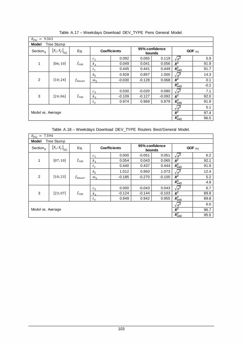
103

Table A.17 – Weekdays Download DEV_TYPE Pens General Model.

𝜎[%] = 9.363

Model Tree Stump



GOF [%]

1 [06; 10] 𝑓𝑒𝑥𝑝

𝑐1 0.092 0.065 0.119 √𝜺𝟐̅̅ ̅ 5.9

𝑘1 0.049 0.041 0.056 𝑹𝟐 91.9

𝑡1 0.445 0.441 0.449 𝑹𝒂𝒅𝒋𝟐 91.7

2 [10; 24] 𝑓𝑙𝑖𝑛𝑒𝑎𝑟

𝑏2 0.928 0.857 1.000 √𝜺𝟐̅̅ ̅ 14.3

𝑚2 -0.030 -0.128 0.068 𝑹𝟐 0.1

𝑹𝒂𝒅𝒋𝟐 -0.2

3 [24; 06] 𝑓𝑒𝑥𝑝

𝑐3 0.030 -0.020 0.080 √𝜺𝟐̅̅ ̅ 7.1

𝑘3 -0.109 -0.127 -0.092 𝑹𝟐 92.0

𝑡3 0.974 0.969 0.979 𝑹𝒂𝒅𝒋𝟐 91.9

Model vs. Average

√𝜺𝟐̅̅ ̅ 5.1

𝑹𝟐 97.4


Table A.18 – Weekdays Download DEV_TYPE Routers Best/General Model.

𝜎[%] = 7.594

Model Tree Stump



GOF [%]

1 [07; 10] 𝑓𝑒𝑥𝑝 𝑐1 0.000 -0.051 0.051 √𝜺𝟐̅̅ ̅ 6.2

𝑘1 0.054 0.043 0.065 𝑹𝟐 92.1

𝑡1 0.440 0.437 0.444 𝑹𝒂𝒅𝒋𝟐 91.9

2 [10; 23] 𝑓𝑙𝑖𝑛𝑒𝑎𝑟

𝑏2 1.012 0.950 1.073 √𝜺𝟐̅̅ ̅ 12.4

𝑚2 -0.185 -0.270 -0.100 𝑹𝟐 5.2


3 [23; 07] 𝑓𝑒𝑥𝑝 𝑐3 0.000 -0.043 0.043 √𝜺𝟐̅̅ ̅ 6.7

𝑘3 -0.124 -0.144 -0.103 𝑹𝟐 89.9

𝑡3 0.949 0.942 0.955 𝑹𝒂𝒅𝒋𝟐 89.8

Model vs. Average

√𝜺𝟐̅̅ ̅ 6.0

𝑹𝟐 96.7


104

Table A.19 – Weekdays Download DEV_TYPE Smartphone Best/General Model.

𝜎[%] = 5.585

Model Tree Stump



GOF [%]

1 [06; 09] 𝑓𝑒𝑥𝑝

𝑐1 0.000 -0.051 0.052 √𝜺𝟐̅̅ ̅ 5.5

𝑘1 0.058 0.047 0.070 𝑹𝟐 94.0

𝑡1 0.402 0.398 0.405 𝑹𝒂𝒅𝒋𝟐 93.9

2 [09; 24] 𝑓𝑙𝑖𝑛𝑒𝑎𝑟

𝑏2 0.681 0.640 0.722 √𝜺𝟐̅̅ ̅ 9.5

𝑚2 0.289 0.231 0.347 𝑹𝟐 20.9


3 [24; 06] 𝑓𝑒𝑥𝑝

𝑐3 0.000 -0.036 0.036 √𝜺𝟐̅̅ ̅ 5.6

𝑘3 -0.105 -0.117 -0.093 𝑹𝟐 95.3

𝑡3 0.978 0.975 0.982 𝑹𝒂𝒅𝒋𝟐 95.2

Model vs. Average

√𝜺𝟐̅̅ ̅ 5.2

𝑹𝟐 97.2


Table A.20 – Weekdays Download DEV_TYPE Tablet Best/General Model.

𝜎[%] = 9.814

Model Tree Stump



GOF [%]

1 [06; 09] 𝑓𝑒𝑥𝑝 𝑐1 0.000 -0.064 0.064 √𝜺𝟐̅̅ ̅ 5.6

𝑘1 0.066 0.044 0.087 𝑹𝟐 84.8

𝑡1 0.430 0.419 0.442 𝑹𝒂𝒅𝒋𝟐 84.5

2 [09; 00] 𝑓𝑙𝑖𝑛𝑒𝑎𝑟

𝑏2 0.189 0.136 0.243 √𝜺𝟐̅̅ ̅ 13.3

𝑚2 0.778 0.704 0.851 𝑹𝟐 52.8


3 [00; 06] 𝑓𝑒𝑥𝑝 𝑐3 0.000 -0.049 0.049 √𝜺𝟐̅̅ ̅ 7.2

𝑘3 -0.087 -0.102 -0.071 𝑹𝟐 90.9

𝑡3 1.012 1.007 1.016 𝑹𝒂𝒅𝒋𝟐 90.8

Model vs. Average

√𝜺𝟐̅̅ ̅ 3.7

𝑹𝟐 98.2


Table A.21 – OP_SYS Best Models: Ranking.

(1)

Android (2)

Others (3)

Windows (4) iOS

WD

D

L 1º TG TG TS TS

2º TS TS T T

WD

U

L 1º TG TG TG TG

2º DG TS T T

WE

D

L 1º TG TS TG TG

2º TS TG TS TS

WE

U

L 1º TG TG TG TG

2º DG TS T T

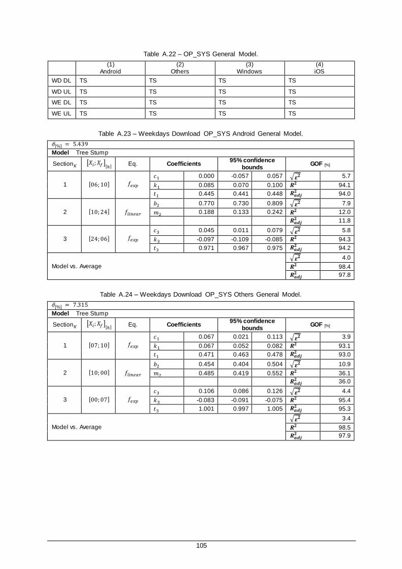
105

Table A.22 – OP_SYS General Model.

(1)

Android (2)

Others (3)

Windows (4) iOS

WD DL TS TS TS TS

WD UL TS TS TS TS

WE DL TS TS TS TS

WE UL TS TS TS TS

Table A.23 – Weekdays Download OP_SYS Android General Model.

𝜎[%] = 5.439

Model Tree Stump



GOF [%]

1 [06; 10] 𝑓𝑒𝑥𝑝 𝑐1 0.000 -0.057 0.057 √𝜺𝟐̅̅ ̅ 5.7

𝑘1 0.085 0.070 0.100 𝑹𝟐 94.1

𝑡1 0.445 0.441 0.448 𝑹𝒂𝒅𝒋𝟐 94.0

2 [10; 24] 𝑓𝑙𝑖𝑛𝑒𝑎𝑟

𝑏2 0.770 0.730 0.809 √𝜺𝟐̅̅ ̅ 7.9

𝑚2 0.188 0.133 0.242 𝑹𝟐 12.0


3 [24; 06] 𝑓𝑒𝑥𝑝

𝑐3 0.045 0.011 0.079 √𝜺𝟐̅̅ ̅ 5.8

𝑘3 -0.097 -0.109 -0.085 𝑹𝟐 94.3

𝑡3 0.971 0.967 0.975 𝑹𝒂𝒅𝒋𝟐 94.2

Model vs. Average

√𝜺𝟐̅̅ ̅ 4.0

𝑹𝟐 98.4


Table A.24 – Weekdays Download OP_SYS Others General Model.

𝜎[%] = 7.315

Model Tree Stump



GOF [%]

1 [07; 10] 𝑓𝑒𝑥𝑝

𝑐1 0.067 0.021 0.113 √𝜺𝟐̅̅ ̅ 3.9

𝑘1 0.067 0.052 0.082 𝑹𝟐 93.1

𝑡1 0.471 0.463 0.478 𝑹𝒂𝒅𝒋𝟐 93.0

2 [10; 00] 𝑓𝑙𝑖𝑛𝑒𝑎𝑟

𝑏2 0.454 0.404 0.504 √𝜺𝟐̅̅ ̅ 10.9

𝑚2 0.485 0.419 0.552 𝑹𝟐 36.1


3 [00; 07] 𝑓𝑒𝑥𝑝

𝑐3 0.106 0.086 0.126 √𝜺𝟐̅̅ ̅ 4.4

𝑘3 -0.083 -0.091 -0.075 𝑹𝟐 95.4

𝑡3 1.001 0.997 1.005 𝑹𝒂𝒅𝒋𝟐 95.3

Model vs. Average

√𝜺𝟐̅̅ ̅ 3.4

𝑹𝟐 98.5


106

Table A.25 – Weekdays Download OP_SYS Windows Best/General Model.

𝜎[%] = 11.633

Model Tree Stump



GOF [%]

1 [06; 09] 𝑓𝑒𝑥𝑝

𝑐1 0.000 -0.065 0.065 √𝜺𝟐̅̅ ̅ 6.9

𝑘1 0.058 0.045 0.072 𝑹𝟐 91.4

𝑡1 0.398 0.395 0.402 𝑹𝒂𝒅𝒋𝟐 91.3

2 [09; 24] 𝑓𝑙𝑖𝑛𝑒𝑎𝑟

𝑏2 0.604 0.535 0.673 √𝜺𝟐̅̅ ̅ 15.9

𝑚2 0.350 0.252 0.447 𝑹𝟐 12.0


3 [24; 06] 𝑓𝑒𝑥𝑝

𝑐3 0.000 -0.080 0.080 √𝜺𝟐̅̅ ̅ 12.2

𝑘3 -0.105 -0.131 -0.080 𝑹𝟐 82.4

𝑡3 0.983 0.975 0.990 𝑹𝒂𝒅𝒋𝟐 82.2

Model vs. Average

√𝜺𝟐̅̅ ̅ 5.5 𝟐 96.6


Table A.26 – Weekdays Download OP_SYS iOS Best/General Model.

𝜎[%] = 5.577

Model Tree Stump



GOF [%]

1 [06; 09] 𝑓𝑒𝑥𝑝 𝑐1 0.016 -0.029 0.062 √𝜺𝟐̅̅ ̅ 5.7

𝑘1 0.052 0.042 0.062 𝑹𝟐 93.9

𝑡1 0.400 0.397 0.403 𝑹𝒂𝒅𝒋𝟐 93.7

2 [09; 24] 𝑓𝑙𝑖𝑛𝑒𝑎𝑟

𝑏2 0.664 0.625 0.702 √𝜺𝟐̅̅ ̅ 8.8

𝑚2 0.320 0.266 0.374 𝑹𝟐 27.2


3 [24; 06] 𝑓𝑒𝑥𝑝 𝑐3 0.000 -0.038 0.038 √𝜺𝟐̅̅ ̅ 6.1

𝑘3 -0.102 -0.114 -0.090 𝑹𝟐 95.0

𝑡3 0.983 0.980 0.987 𝑹𝒂𝒅𝒋𝟐 94.9

Model vs. Average

√𝜺𝟐̅̅ ̅ 4.8

𝑹𝟐 97.7


107

References [1] 3GPP, Radio Access Milestones, http://www.3gpp.org/about -3gpp, Jan. 2016.

[2] Ericsson, Ericsson Mobility Report, Ericsson, Stockholm, Sweden, Nov. 2016

(https://www.ericsson.com/assets/local/mobility-report/documents/2016/ericsson-mobility-

report-november-2016.pdf).

[3] Y. Ouyang, M.H. Fallah, S. Hu, Y. Yong Ren, Y. Hu, Z. Lai, M. Guan, and W.D. Lu, “A novel

methodology of data analytics and modeling to evaluate LTE network performance”, in Proc. of

WTS’14 - 13th IEEE Wireless Telecommunications Symposium, Washington, D.C., USA, Apr.

2014 (http://ieeexplore.ieee.org/stamp/stamp.jsp?tp=&arnumber=6835006).

[4] S.K. Baghel, K. Keshav, and V.R. Manepalli, “An investigation into traffic analysis for diverse

data applications on smartphones”, in Proc. of NCC’12 - 2012 IEEE National Conference on

Communications, Kharagpur, India, Feb. 2012

(http://ieeexplore.ieee.org/stamp/stamp.jsp?tp=&arnumber=6176903).

[5] Ericsson, Ericsson Mobility Report, Ericsson, Stockholm, Sweden, Jun. 2015

(http://www.ericsson.com/res/docs/2015/ericsson-mobility-report-june-2015.pdf).

[6] 3GPP, UTRAN Overall Description (Release 14), Report TS 25.401 V14.0.0, Technical

Specification Group Radio Access Network, 3GPP, Valbonne, France, Mar. 2017

(http://www.3gpp.org/ftp//Specs/archive/25_series/25.401/).

[7] H. Holma and A. Toskala, WCDMA for UMTS (5th Edition), John Wiley & Sons, Chichester, UK,

2010.

[8] A.F. Molisch, Wireless Communications, John Wiley & Sons, Chichester, UK, 2011.

[9] L.M. Correia, Mobile Communication Systems, Lecture Notes, Instituto Superior Tecnico,

Technical University of Lisbon, Lisbon, Portugal, 2015

(http://fenix.tecnico.ulisboa.pt/disciplinas/SCM364511/2014 -2015/2-semestre).

[10] H. Holma and A. Toskala, LTE for UMTS: Evolution to LTE Advanced (2nd Edition), John Wiley

& Sons, Chichester, UK, 2011.

[11] S. Sesia, I. Toufik, and I. Baker, LTE - The UMTS Long Term Evolution: From Theory to Practice

(2nd Edition), John Wiley & Sons, Chichester, UK, 2011.

[12] M. Sá, Performance Analysis of Software Defined Networks in LTE-A, M.Sc. Thesis, Instituto

Superior Tecnico, Technical University of Lisbon, Lisbon, Portugal, 2015 (http://grow.inov.pt /wp -

content/uploads/2015/08/Thesis_MiguelSa_FinalVersion.pdf).

[13] ANACOM, Final Report Auction (in Portuguese), ANACOM, Lisbon, Portugal, Jan. 2012

(https://www.anacom.pt/render.jsp?contentId=1112758).

[14] E. Dahlman, S. Parkvall, and J. Sköld, 4G LTE/LTE-Advanced for Mobile Broadband, Academic

108

Press, Oxford, UK, 2011.

[15] Z. Zhang, Z. Zhao, H. Guan, D. Laselva, D.I. Park, K.M. Hwang, D.H. Kim, and Z. Tan, “A novel

traffic generation framework for LTE network evolution study”, in Proc. of PIMRC’14 - 25th IEEE

Annual International Symposium on Personal, Indoor, and Mobile Radio Communication,

Washington, D.C., USA, Sep. 2014


[16] 3GPP, Policy and charging control architecture (Release 14), Report TS 23.203 V14.3.0,

Technical Specification Group Services and System Aspects, 3GPP, Valbonne, France, Mar.

2017 (http://www.3gpp.org/ftp//Specs/archive/23_series/23.203/).

[17] K. Sina, Radio Resource Management Strategies in Virtual Networks , Ph.D. Thesis, Instituto

Superior Tecnico, Technical University of Lisbon, Lisbon, Portugal, 2016

(http://grow.tecnico.ulisboa.pt/user/skhatibi/).

[18] Huawei Technologies, Smartphone Solutions, White Paper, Prepared by Smartphone

ecosystem R&D support team, Issue 2.0, Huawei Technologies, Shenzhen, China, Jul. 2012

(www.huawei.com/ilink/en/download/HW_193034).

[19] P. Pastor, F. Fradella, A. Ravagnolo, and P. Valenza, Conceptual approach for a mobile BU-

LRIC model, Report for ICP-ANACOM, Public Version, Reference 2002126-153, Analysys

Mason Limited, London, UK, Apr. 2015

(http://www.anacom.pt/streaming/anexo3_MTRmodelconceptpaper.pdf?contentId=1354319&fi

eld=ATTACHED_FILE).

[20] ANACOM, Network Dimensioning - Geographic Characterisation,

http://www.anacom.pt/render.jsp?category Id=381856&cat=381862, in Portuguese, Mar. 2016.

[21] P. Pastor, F. Fradella, A. Ravagnolo, and P. Valenza, Bottom-up mobile cost model update,

Report for ICP-ANACOM, Public Version, Reference 2002126-153, Model documentation,

Analysys Mason Limited, London, UK, Apr. 2015

(http://www.anacom.pt/streaming/anexo2_MTRmodeldocumentation.pdf?content Id=1354318&f

ield=ATTACHED_FILE).

[22] P. Pastor, F. Fradella, A. Ravagnolo, and P. Valenza, Update of the mobile LRIC model: change

report, Report for ICP-ANACOM, Public Version, Reference 2002126-153, Analysys Mason

Limited, London, UK, Apr. 2015

(http://www.anacom.pt/streaming/anexo4_MTRmodelupdate.pdf?contentId=1354320&field=AT

TACHED_FILE).

[23] M. Afanasyev, T. Chen, G.M. Voelker, and A.C. Snoeren, “Usage Patterns in an Urban WiFi

Network”, IEEE/ACM Transactions on Network ing, Vol. 18, No. 5, Oct. 2010, pp. 1359–1372

(http://ieeexplore.ieee.org/lpdocs/epic03/wrapper.htm?arnumber=5401061).

[24] L. Korowajczuk, How to Dimension User Traffic in 4G Networks , CelPlan Technologies, Reston,

VA, USA, Jun. 2014 (http://www.celplan.com/webinars/How to Dimension User Traffic in 4G

Networks rev13.pdf).

109

[25] R.A. Kalden, Mobile Internet Traffic Measurement and Modeling Based on Data From

Commercial GPRS Networks, Ph.D. Thesis, University of Twente, Twente, Netherlands, 2004

(http://doc.utwente.nl/48238/1/thesis_kalden.pdf).

[26] S. Almeida and J. Queijo, Spatial and Temporal Traffic Distributions Models for GSM (in

Portuguese), Diploma Thesis, Instituto Superior Tecnico, Technical University of Lisbon, Lisbon,

Portugal, 1998 (http://grow.inov.pt/wp-content/uploads/2014/01/SandraJose_Lic_1998.pdf).

[27] D. Silva, Energy efficient solutions in GSM/UMTS based on traffic profiling models , M.Sc. Thesis,

Instituto Superior Tecnico, Technical University of Lisbon, Lisbon, Portugal, 2012

(http://grow.inov.pt/wp-content/uploads/2014/01/DiogoSilva_MSc_2012final.pdf).

[28] H. Motulsky and A. Christopoulos, Fitting Models to Biological Data Using Linear and Nonlinear

Regression: A Practical Guide to Curve Fitting, Oxford University Press, Oxford, UK, 2004.

[29] L. Guan, X. Zhang, Z. Liu, Y. Huang, R. Lan, and W. Wang, “Spatial modeling and analysis of

traffic distribution based on real data from current mobile cellular networks”, in Proc. of ICCP’13

- 2013 IEEE International Conference on Computational Problem-Solving, Jiuzhai, China, Oct.

2013 (http://ieeexplore.ieee.org/lpdocs/epic03/wrapper.htm?arnumber=6893524).

[30] S. Park and J. Kim, “Effect of LTE service adoption on mobile data traffic in Korea”, in Proc. of

ICCCT’12 - 7th IEEE International Conference on Computing and Convergence Technology ,

Seoul, South Korea, Dec. 2012


[31] H. Khedher, F. Valois, and S. Tabbane, “Traffic characterisation for mobile networks”, in Proc. of

VTC’02-Fall - 56th IEEE Vehicular Technology Conference, Vancouver, Canada, Sep. 2002


[32] EARTH, Energy efficiency analysis of the reference systems, areas of improvements and target

breakdown, INFSO-ICT-247733 EARTH, Deliverable D2.3, EARTH, Jan. 2012 (https://www.ict -

earth.eu/publications/deliverables/deliverables.html).

[33] G. Micallef, “Methods for Reducing the Energy Consumption of Mobile Broadband Networks”,

Telektronikk , No. 1, 2010, pp. 121–128.

[34] Z. Zhu, G. Cao, R. Keralapura, and A. Nucci, “Characterising Data Services in a 3G Network:

Usage, Mobility and Access Issues”, in Proc. of ICC’11 - 2011 IEEE International Conference on

Communications, Kyoto, Japan, Jun. 2011


[35] UMTS Forum, Mobile traffic forecasts 2010-2020 report, UMTS Forum Report 44, UMTS Forum,

London, UK, Jan. 2011 (http://www.umts-

forum.org/component/option,com_docman/task,cat_view/gid,485/Itemid,213/).

[36] Q. Xu, J. Erman, A. Gerber, Z. Mao, J. Pang, and S. Venkataraman, “Identifying Diverse Usage

Behaviors of Smartphone Apps”, in Proc. of IMC’11 - 2011 ACM/SIGCOMM Internet

Measurement Conference, Berlin, Germany, Nov. 2011

110

(https://web.eecs.umich.edu/~zmao/Papers/imc11_xu.pdf).

[37] M. Boulmalf, J. Abrache, T. Aouam, and H. Harroud, “Traffic analysis for GSM networks”, in Proc.

of AICCSA’09 - 2009 IEEE/ACS International Conference on Computer Systems and

Applications, Rabat, Morocco, May 2009


[38] Vodafone Portugal, Vodafone Hotspot 4G, https://loja.vodafone.pt/tablets -pens-

hotspots/vodafone/hotspot-4g-r216-cartao-gratuito-branco, Mar. 2017.

[39] Vodafone Portugal, Vodafone Pen 4G, https://loja.vodafone.pt/tablets-pens-

hotspots/vodafone/pen-4g-k5160-cartao-gratuito-branco, Mar. 2017.

[40] Vodafone Portugal, Vodafone Router 4G, https://negocios.vodafone.pt/loja/tablets -pens-

hotspots/vodafone/router-4g-b4000-branco, Mar. 2017.

[41] D.C. Montgomery and G.C. Runger, Applied Statistics and Probability for Engineers, 6th Edition,

John Wiley & Sons, Inc., Hoboken, NJ, USA, 2014.

[42] S. McKillup, Statistics Explained: An Introductory Guide for Life Scientists, 2nd Edition,

Cambridge University Press, Cambridge, UK, 2011.

[43] MathWorks, Lilliefors test, https://www.mathworks.com/help/stats/lillietest.html, MATLAB

R2016a Documentation, Apr. 2016.

[44] J. Sá, Applied Statistics Using SPSS, STATISTICA, MATLAB and R, Springer Berlin Heidelberg,

Berlin, Germany, 2007.

[45] M. Lovric, International Encyclopedia of Statistical Science, Springer Berlin Heidelberg, Berlin,

Heidelberg, 2011.

[46] MathWorks, Evaluating Goodness of Fit, https://www.mathworks.com/help/curvefit/ evaluat ing-

goodness-of-fit.html, MATLAB R2016a Documentation, Apr. 2016.

[47] S.M. Ross, Introduction to probability and statistics for engineers and scientists, 4th Edition ,

Elsevier/Academic Press, Burlington, MA, USA, 2009.

[48] M.C. Morais, Probability and Statistics, Lecture Notes, Instituto Superior Tecnico, Technical

University of Lisbon, Lisbon, Portugal, 2010.

[49] M. Holický, Introduction to Probability and Statistics for Engineers , Springer Berlin Heidelberg,

Berlin, Germany, 2013.

[50] MathWorks, Interp1, https://www.mathworks.com/help/matlab/ref/interp1.html, MATLAB

R2016a Documentation, Apr. 2016.

[51] MathWorks, Fit, https://www.mathworks.com/help/curvefit/fit.html, MATLAB R2016a

Documentation, Apr. 2016.

Temporal Modelling of Mobile Data Traffic Applications

Documents

Transcript of Temporal Modelling of Mobile Data Traffic Applications