Modelling spatio-temporal data with R - Geoinformaticspebesma.staff.ifgi.de/inpe.pdf · Modelling...
57
Why R? R spatial R temporal R spatio-temporal Conclusions Modelling spatio-temporal data with R Edzer Pebesma ifgi Institute for Geoinformatics University of Münster [email protected] GeoINFO, Nov 29 – Dec 1, 2010, Campos do Jord˜ ao (SP) One-day bilateral research workshop at INPE, Dec 2, 2010, S˜ ao Jos´ e dos Campos (SP)
Transcript of Modelling spatio-temporal data with R - Geoinformaticspebesma.staff.ifgi.de/inpe.pdf · Modelling...
Why R? R spatial R temporal R spatio-temporal Conclusions
Modelling spatio-temporal data with R
Edzer Pebesma
1. Das neue IfGI-Logo 1.6 Logovarianten
Logo für den Einsatz in internationalen bzw.
englischsprachigen Präsentationen.
Einsatzbereiche: Briefbogen, Visitenkarte,
Titelblätter etc.
Mindestgröße 45 mm Breite
ifgi
ifgi
Institute for GeoinformaticsUniversity of Münster
ifgi
Institut für GeoinformatikUniversität Münster
Logo für den Einsatz in nationalen bzw.
deutschsprachigen Präsentationen.
Einsatzbereiche: Briefbogen, Visitenkarte,
Titelblätter etc.
Mindestgröße 45 mm Breite
Dieses Logo kann bei Anwendungen
eingesetzt werden, wo das Logo besonders
klein erscheint.
Einsatzbereiche: Sponsorenlogo,
Power-Point
Größe bis 40 mm Breite
GeoINFO, Nov 29 – Dec 1, 2010, Campos do Jordao (SP)One-day bilateral research workshop at INPE, Dec 2, 2010, Sao Jose
dos Campos (SP)
Why R? R spatial R temporal R spatio-temporal Conclusions
Overview
1 Why R?
2 R spatial
3 R temporal
4 R spatio-temporal
5 Conclusions
Why R? R spatial R temporal R spatio-temporal Conclusions
Outline
Why R?
R for spatial data analysis
R for temporal data analysis
Spatio-temporal data types, processes, models
R infrastructure for spatio-temporal data analysis
outlook
Joint work with Roger Bivand, and with help from Michael Sumnerand many people at r-sig-geo.
Why R? R spatial R temporal R spatio-temporal Conclusions
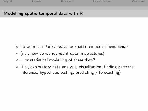
Modelling spatio-temporal data with R
do we mean data models for spatio-temporal phenomena?
(i.e., how do we represent data in structures)
.. or statistical modelling of these data?
(i.e., exploratory data analysis, visualisation, finding patterns,inference, hypothesis testing, predicting / forecasting)
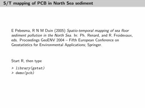
S/T mapping of PCB in North Sea sediment
E Pebesma, R N M Duin (2005) Spatio-temporal mapping of sea floorsediment pollution in the North Sea. In: Ph. Renard, and R. Froidevaux,eds. Proceedings GeoENV 2004 – Fifth European Conference onGeostatistics for Environmental Applications; Springer.
Start R, then type
> library(gstat)
> demo(pcb)

Easy manipulation of data objects
> A = log(pcb[pcb$year == 1991, "PCB138"])
> B = log(pcb[pcb$year == 1986, "PCB138"])
> cor(A, B)

Handling missing values
missing values are part of everyreal data set, and if not
they get created along the way(cloud removal in RS imagery)
in low-level programming,handling them properly take alot of energy ...
in particular, across all basictypes (int, byte, boolean, float,char, ...)
> 1/0
[1] Inf
> log(0)
[1] -Inf
> 0/0
[1] NaN
> as.numeric(NA)
[1] NA
> is.nan(NA)
[1] FALSE
> is.na(NA)
[1] TRUE
> mean(c(1, 2, 3, NA))
[1] NA
> mean(c(1, 2, 3, NA), na.rm = TRUE)
[1] 2
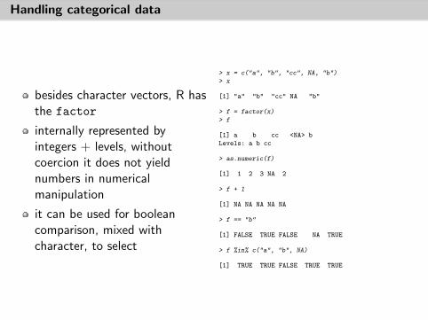
Handling categorical data
besides character vectors, R hasthe factor
internally represented byintegers + levels, withoutcoercion it does not yieldnumbers in numericalmanipulation
it can be used for booleancomparison, mixed withcharacter, to select
> x = c("a", "b", "cc", NA, "b")
> x
[1] "a" "b" "cc" NA "b"
> f = factor(x)
> f
[1] a b cc <NA> b
Levels: a b cc
> as.numeric(f)
[1] 1 2 3 NA 2
> f + 1
[1] NA NA NA NA NA
> f == "b"
[1] FALSE TRUE FALSE NA TRUE
> f %in% c("a", "b", NA)
[1] TRUE TRUE FALSE TRUE TRUE
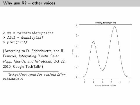
Why use R? – other voices
> xx = faithful$eruptions
> fit1 = density(xx)
> plot(fit1)
(According to D. Eddenbuettel and R
Francois, Integrating R with C++:
Rcpp, RInside, and RProtobuf, Oct 22,
2010, Google TechTalka)
ahttp://www.youtube.com/watch?v=
UZkaZhsOfT41 2 3 4 5 6
0.0
0.1
0.2
0.3
0.4
0.5
density.default(x = xx)
N = 272 Bandwidth = 0.3348
Den
sity
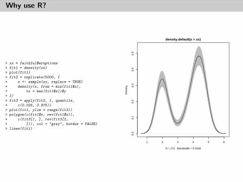
Why use R?
> xx = faithful$eruptions
> fit1 = density(xx)
> plot(fit1)
> fit2 = replicate(5000, {
+ x <- sample(xx, replace = TRUE)
+ density(x, from = min(fit1$x),
+ to = max(fit1$x))$y
+ })
> fit3 = apply(fit2, 1, quantile,
+ c(0.025, 0.975))
> plot(fit1, ylim = range(fit3))
> polygon(c(fit1$x, rev(fit1$x)),
+ c(fit3[1, ], rev(fit3[2,
+ ])), col = "grey", border = FALSE)
> lines(fit1)
1 2 3 4 5 6
0.0
0.1
0.2
0.3
0.4
0.5
density.default(x = xx)
N = 272 Bandwidth = 0.3348
Den
sity
Why R? R spatial R temporal R spatio-temporal Conclusions
R is not meant as a data base
Typically,
R sessions start with importing data from a (file, data base,web service)
a number of commands are executed to reach (or get nearerto) a goal
output is saved (to file, data base, graph, table,...)
the set of R commands (.Rhistory) is cleaned, saved to a .Rscript file, and checked, to safe the analysis forcommunication or future use.
(R objects do not have a history, nor time stamps)

Why R? R spatial R temporal R spatio-temporal Conclusions
It’s the combination of
having everything in one place:
data manipulation / selection options
functionality from linear algebra to modelling
NA, factors, time
arrays, matrices
easy to convert complex data in useful plots
professional quality graphics to a variety of devices
2650 extension packages on CRAN for research dissemination
Sweave: removes need to cut and paste, guaranteesconsistency
(arguably:) lingua franca of statistical computation

Why R? R spatial R temporal R spatio-temporal Conclusions
R spatial

Before 2005
R
spatstat
maptools
splancs
spdep
geoR
gstat
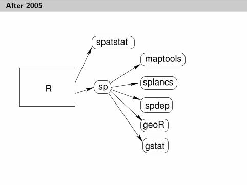
After 2005
maptools
sp splancs
spdep
geoR
gstat
R
spatstat

2010
maptools
sp splancs
spdep
geoR
gstat
R
spatstat
+40
rgdal
sos4R

Classes in sp
data type class attributes containspoints SpatialPoints No Spatial*points SpatialPointsDataFrame data.frame SpatialPoints*pixels SpatialPixels No SpatialPoints*pixels SpatialPixelsDataFrame data.frame SpatialPixels*
SpatialPointsDataFrame**full grid SpatialGrid No SpatialPixels*full grid SpatialGridDataFrame data.frame SpatialGrid*line Line Nolines Lines No Line listlines SpatialLines No Spatial*, Lines listlines SpatialLinesDataFrame data.frame SpatialLines*rings Polygon No Line*rings Polygons No Polygon listrings SpatialPolygons No Spatial*, Polygons listrings SpatialPolygonsDataFrame data.frame SpatialPolygons*
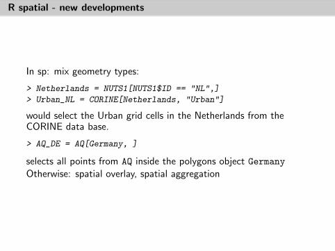
R spatial - new developments
In sp: mix geometry types:
> Netherlands = NUTS1[NUTS1$ID == "NL",]
> Urban_NL = CORINE[Netherlands, "Urban"]
would select the Urban grid cells in the Netherlands from theCORINE data base.
> AQ_DE = AQ[Germany, ]
selects all points from AQ inside the polygons object GermanyOtherwise: spatial overlay, spatial aggregation
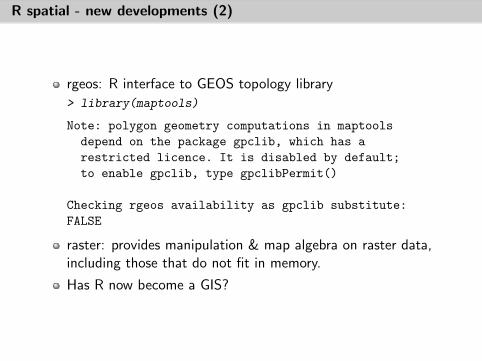
R spatial - new developments (2)
rgeos: R interface to GEOS topology library
> library(maptools)
Note: polygon geometry computations in maptools
depend on the package gpclib, which has a
restricted licence. It is disabled by default;
to enable gpclib, type gpclibPermit()
Checking rgeos availability as gpclib substitute:
FALSE
raster: provides manipulation & map algebra on raster data,including those that do not fit in memory.
Has R now become a GIS?
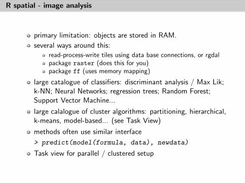
R spatial - image analysis
primary limitation: objects are stored in RAM.
several ways around this:
read-process-write tiles using data base connections, or rgdalpackage raster (does this for you)package ff (uses memory mapping)
large catalogue of classifiers: discriminant analysis / Max Lik;k-NN; Neural Networks; regression trees; Random Forest;Support Vector Machine...
large calalogue of cluster algorithms: partitioning, hierarchical,k-means, model-based... (see Task View)
methods often use similar interface
> predict(model(formula, data), newdata)
Task view for parallel / clustered setup
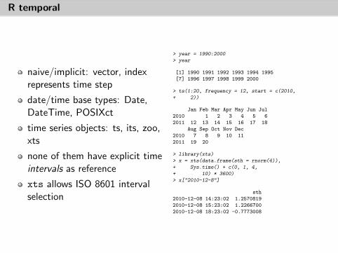
R temporal
naive/implicit: vector, indexrepresents time step
date/time base types: Date,DateTime, POSIXct
time series objects: ts, its, zoo,xts
none of them have explicit timeintervals as reference
xts allows ISO 8601 intervalselection
> year = 1990:2000
> year
[1] 1990 1991 1992 1993 1994 1995
[7] 1996 1997 1998 1999 2000
> ts(1:20, frequency = 12, start = c(2010,
+ 2))
Jan Feb Mar Apr May Jun Jul
2010 1 2 3 4 5 6
2011 12 13 14 15 16 17 18
Aug Sep Oct Nov Dec
2010 7 8 9 10 11
2011 19 20
> library(xts)
> x = xts(data.frame(sth = rnorm(4)),
+ Sys.time() + c(0, 1, 4,
+ 10) * 3600)
> x["2010-12-8"]
sth
2010-12-08 14:23:02 1.2570819
2010-12-08 15:23:02 1.2266700
2010-12-08 18:23:02 -0.7773008
Why R? R spatial R temporal R spatio-temporal Conclusions
Statistical analysis of spatio-temporal data
Questions to data often involve the words where and when, eitherimplicitly (through covariates / predictors: under whichcircumstances) or explicitly (i.e., there [location] / then [time])Statistical modelling proceeds, as usual, along the line of splittingvariability in an understood and a random component (possibly:smooth + rough):
observation = trend + residual
where often the non-random trend relates copes with covariates,and the random residual with correlations in space and time.
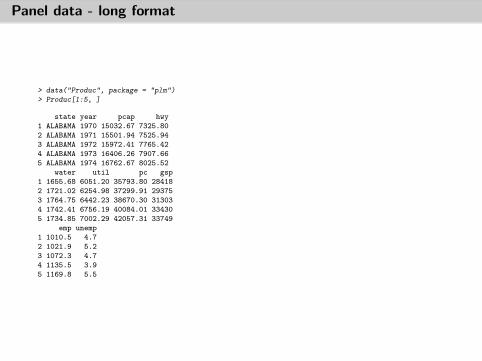
Panel data - long format
> data("Produc", package = "plm")
> Produc[1:5, ]
state year pcap hwy
1 ALABAMA 1970 15032.67 7325.80
2 ALABAMA 1971 15501.94 7525.94
3 ALABAMA 1972 15972.41 7765.42
4 ALABAMA 1973 16406.26 7907.66
5 ALABAMA 1974 16762.67 8025.52
water util pc gsp
1 1655.68 6051.20 35793.80 28418
2 1721.02 6254.98 37299.91 29375
3 1764.75 6442.23 38670.30 31303
4 1742.41 6756.19 40084.01 33430
5 1734.85 7002.29 42057.31 33749
emp unemp
1 1010.5 4.7
2 1021.9 5.2
3 1072.3 4.7
4 1135.5 3.9
5 1169.8 5.5
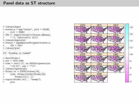
Panel data as ST structure
> library(maps)
> states.m = map("state", plot = FALSE,
+ fill = TRUE)
> IDs <- sapply(strsplit(states.m$names,
+ ":"), function(x) x[1])
> library(maptools)
> states = map2SpatialPolygons(states.m,
+ IDs = IDs)
> library(plm)
[1] "kinship is loaded"
> data(Produc)
> yrs = 1970:1986
> time = xts(1:17, as.POSIXct(paste(yrs,
+ "-01-01", sep = "")))
> library(spacetime)
> Produc.st = STFDF(states[-8],
+ time, Produc[(order(Produc[2],
+ Produc[1])), ])
> stplot(Produc.st[, , "unemp"],
+ yrs)
1970 1971 1972
1973 1974 1975
1976 1977 1978
1979 1980 1981
1982 1983 1984
1985 1986
2
4
6
8
10
12
14
16
18
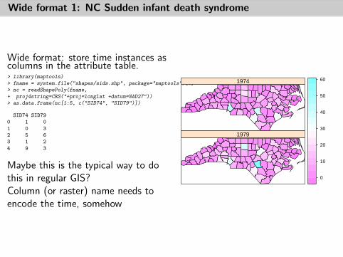
Wide format 1: NC Sudden infant death syndrome
Wide format: store time instances ascolumns in the attribute table.> library(maptools)
> fname = system.file("shapes/sids.shp", package="maptools")[1]
> nc = readShapePoly(fname,
+ proj4string=CRS("+proj=longlat +datum=NAD27"))
> as.data.frame(nc[1:5, c("SID74", "SID79")])
SID74 SID79
0 1 0
1 0 3
2 5 6
3 1 2
4 9 3
Maybe this is the typical way to dothis in regular GIS?Column (or raster) name needs toencode the time, somehow
1974
1979
0
10
20
30
40
50
60
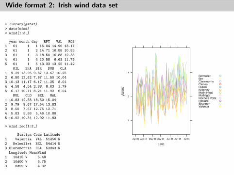
Wide format 2: Irish wind data set
> library(gstat)
> data(wind)
> wind[1:5,]
year month day RPT VAL ROS
1 61 1 1 15.04 14.96 13.17
2 61 1 2 14.71 16.88 10.83
3 61 1 3 18.50 16.88 12.33
4 61 1 4 10.58 6.63 11.75
5 61 1 5 13.33 13.25 11.42
KIL SHA BIR DUB CLA
1 9.29 13.96 9.87 13.67 10.25
2 6.50 12.62 7.67 11.50 10.04
3 10.13 11.17 6.17 11.25 8.04
4 4.58 4.54 2.88 8.63 1.79
5 6.17 10.71 8.21 11.92 6.54
MUL CLO BEL MAL
1 10.83 12.58 18.50 15.04
2 9.79 9.67 17.54 13.83
3 8.50 7.67 12.75 12.71
4 5.83 5.88 5.46 10.88
5 10.92 10.34 12.92 11.83
> wind.loc[1:3,]
Station Code Latitude
1 Valentia VAL 51d56'N
2 Belmullet BEL 54d14'N
3 Claremorris CLA 53d43'N
Longitude MeanWind
1 10d15'W 5.48
2 10d00'W 6.75
3 8d59'W 4.32
1961
spee
d1
2
3
Apr 01 Apr 15 May 01 May 15 Jun 01 Jun 15 Jul 01
BelmulletBirrClaremorrisClonesDublinKilkennyMalin HeadMullingarRoche's PointRoslareShannonValentia
●
●
●
●
●
●
●
●
●
●
●
●
●
●
●
●
●
●
●
●
●
●
●
●
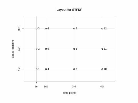
Time points
Spa
ce lo
catio
ns
1st 2nd 3rd 4th
1st
2nd
3rd
1
2
3
4
5
6
7
8
9
10
11
12
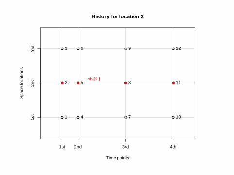
Layout for STFDF
●
●
●
●
●
●
●
●
●
●
●
●
Time points
Spa
ce lo
catio
ns
1st 2nd 3rd 4th
1st
2nd
3rd
1
2
3
4
5
6
7
8
9
10
11
12
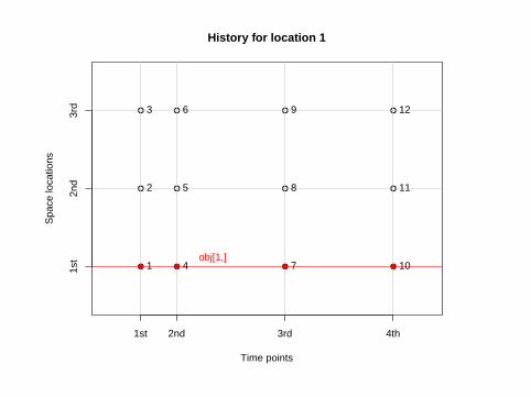
History for location 1
obj[1,]● ● ● ●
●
●
●
●
●
●
●
●
●
●
●
●
Time points
Spa
ce lo
catio
ns
1st 2nd 3rd 4th
1st
2nd
3rd
1
2
3
4
5
6
7
8
9
10
11
12
History for location 2
obj[2,]● ● ● ●
●
●
●
●
●
●
●
●
●
●
●
●
Time points
Spa
ce lo
catio
ns
1st 2nd 3rd 4th
1st
2nd
3rd
1
2
3
4
5
6
7
8
9
10
11
12
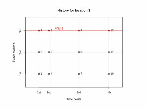
History for location 3
obj[3,]● ● ● ●
●
●
●
●
●
●
●
●
●
●
●
●
Time points
Spa
ce lo
catio
ns
1st 2nd 3rd 4th
1st
2nd
3rd
1
2
3
4
5
6
7
8
9
10
11
12
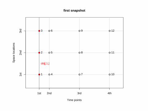
first snapshot
obj[,1,]
●
●
●

●
●
●
●
●
●
●
●
●
●
●
●
Time points
Spa
ce lo
catio
ns
1st 2nd 3rd 4th
1st
2nd
3rd
1
2
3
4
5
6
7
8
9
10
11
12
second snapshot
obj[,2,]
●
●
●
●
●
●
●
●
●
●
●
●
●
●
●
Time points
Spa
ce lo
catio
ns
1st 2nd 3rd 4th
1st
2nd
3rd
1
2
3
4
5
6
7
8
9
10
11
12
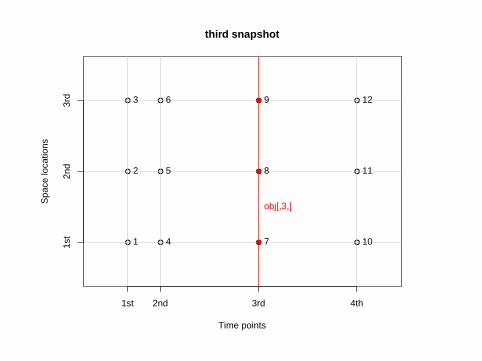
third snapshot
obj[,3,]
●
●
●
●
●
●
●
●
●
●
●
●
●
●
●
Time points
Spa
ce lo
catio
ns
1st 2nd 3rd 4th
1st
2nd
3rd
1
2
3
4
5
6
7
8
9
10
11
12
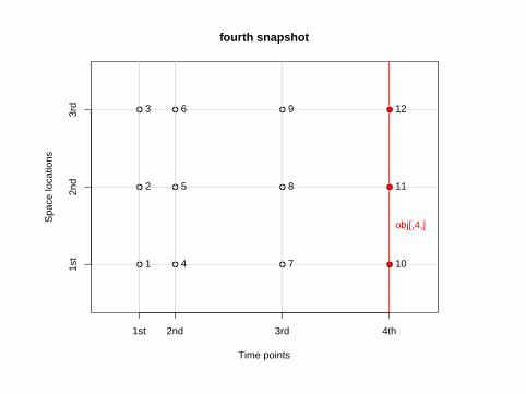
fourth snapshot
obj[,4,]
●
●
●

●
●
●
●
●
●
●
●
●
●
●
●
Time points
Spa
ce lo
catio
ns
1st 2nd 3rd 4th
1st
2nd
3rd
1[1,1]
2[2,1]
3[3,1]
4[2,2]
5[3,2]
6[1,3]
7[2,4]
Layout for STPDF
●
●
●
●
●
Time points
Spa
ce lo
catio
ns
1st 2nd 3rd,4th 5th
1st,4
th2n
d3r
d5t
h
1
2
3
4
5
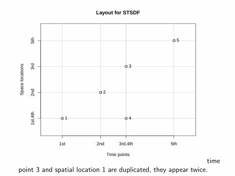
Layout for STSDF
timepoint 3 and spatial location 1 are duplicated, they appear twice.
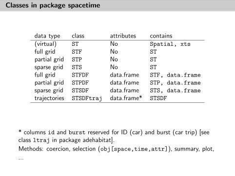
Classes in package spacetime
data type class attributes contains(virtual) ST No Spatial, xts
full grid STF No ST
partial grid STP No ST
sparse grid STS No ST
full grid STFDF data.frame STF, data.frame
partial grid STPDF data.frame STP, data.frame
sparse grid STSDF data.frame STS, data.frame
trajectories STSDFtraj data.frame* STSDF
* columns id and burst reserved for ID (car) and burst (car trip) [seeclass ltraj in package adehabitat].
Methods: coercion, selection (obj[space,time,attr]), summary, plot,
...
●
●
●
●
●
Time points
Spa
ce lo
catio
ns
1st 2nd 3rd,4th 5th
1st,4
th2n
d3r
d5t
h
1
2
3
4
5
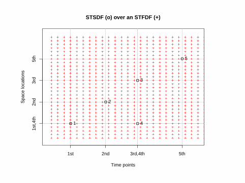
STSDF (o) over an STFDF (+)

Space/time interpolation of Irish wind data
> library(maptools)
> library(mapdata)
> m = map2SpatialLines(map("worldHires",
+ xlim = c(-11,-5.4), ylim = c(51,55.5), plot=F))
> proj4string(m) = "+proj=longlat +datum=WGS84"
> m = spTransform(m, utm29)
> # setup grid
> grd = SpatialPixels(SpatialPoints(makegrid(m, n = 300)),
+ proj4string = proj4string(m))
> # select april 1961:
> w = w[, "1961-04"]
> # 10 prediction time points, evenly spread over this month:
> n = 9
> tgrd = xts(1:n, seq(min(index(w)), max(index(w)), length=n))
> # use separable covariance model,
> # exponential with ranges 750 km and 1.5 day:
> v = list(space = vgm(0.6, "Exp", 750000),
+ time = vgm(1, "Exp", 1.5 * 3600 * 24))
> pred = krigeST(sqrt(values)~1, w, STF(grd, tgrd), v)
> wind.ST = STFDF(grd, tgrd,
+ data.frame(sqrt_speed = pred))
1961−04−01 12:00:001961−04−05 03:00:001961−04−08 18:00:00
1961−04−12 09:00:001961−04−16 00:00:001961−04−19 15:00:00
1961−04−23 06:00:001961−04−26 21:00:001961−04−30 12:00:00
1.1
1.2
1.3
1.4
1.5
1.6
1.7
1.8
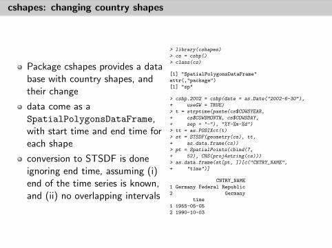
cshapes: changing country shapes
Package cshapes provides a database with country shapes, andtheir change
data come as aSpatialPolygonsDataFrame,with start time and end time foreach shape
conversion to STSDF is doneignoring end time, assuming (i)end of the time series is known,and (ii) no overlapping intervals
> library(cshapes)
> cs = cshp()
> class(cs)
[1] "SpatialPolygonsDataFrame"
attr(,"package")
[1] "sp"
> cshp.2002 = cshp(date = as.Date("2002-6-30"),
+ useGW = TRUE)
> t = strptime(paste(cs$COWSYEAR,
+ cs$COWSMONTH, cs$COWSDAY,
+ sep = "-"), "%Y-%m-%d")
> tt = as.POSIXct(t)
> st = STSDF(geometry(cs), tt,
+ as.data.frame(cs))
> pt = SpatialPoints(cbind(7,
+ 52), CRS(proj4string(cs)))
> as.data.frame(st[pt, ])[c("CNTRY_NAME",
+ "time")]
CNTRY_NAME
1 Germany Federal Republic
2 Germany
time
1 1955-05-05
2 1990-10-03

Why R? R spatial R temporal R spatio-temporal Conclusions
Spatial geometry changing continuously over time
Use case: space-time prisms, alibi problem, meeting planning (PhDWalied Othman)
Time
Space
(linear)

Why R? R spatial R temporal R spatio-temporal Conclusions
Spatial geometry changing continuously over time
Use case: space-time prisms, alibi problem, meeting planning (PhDWalied Othman)
Time
Space
(linear)

Why R? R spatial R temporal R spatio-temporal Conclusions
Spatial and/or temporal support
for spatial nor temporal data, the support (physical size) ofmeasurements is explicitly available
implicit assumptions for spatial spatial: point = 0, grid cell isgrid cell size; line / polygon idem;
implicit assumption for time: length of time step, or explicit(e.g. in Open/High/Low/Close).
Why R? R spatial R temporal R spatio-temporal Conclusions
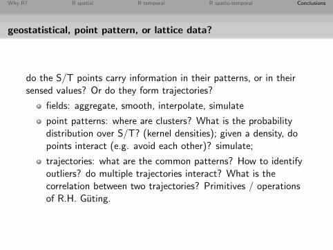
geostatistical, point pattern, or lattice data?
do the S/T points carry information in their patterns, or in theirsensed values? Or do they form trajectories?
fields: aggregate, smooth, interpolate, simulate
point patterns: where are clusters? What is the probabilitydistribution over S/T? (kernel densities); given a density, dopoints interact (e.g. avoid each other)? simulate;
trajectories: what are the common patterns? How to identifyoutliers? do multiple trajectories interact? What is thecorrelation between two trajectories? Primitives / operationsof R.H. Guting.
Why R? R spatial R temporal R spatio-temporal Conclusions
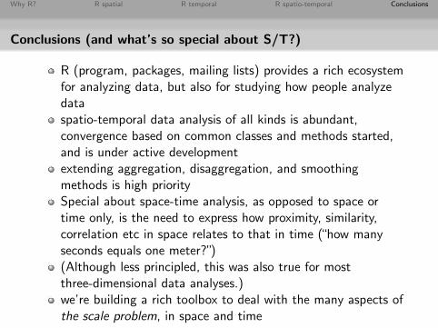
Conclusions (and what’s so special about S/T?)
R (program, packages, mailing lists) provides a rich ecosystemfor analyzing data, but also for studying how people analyzedataspatio-temporal data analysis of all kinds is abundant,convergence based on common classes and methods started,and is under active developmentextending aggregation, disaggregation, and smoothingmethods is high prioritySpecial about space-time analysis, as opposed to space ortime only, is the need to express how proximity, similarity,correlation etc in space relates to that in time (“how manyseconds equals one meter?”)(Although less principled, this was also true for mostthree-dimensional data analyses.)we’re building a rich toolbox to deal with the many aspects ofthe scale problem, in space and time