SPACECRAFT DOPPLER TRACKING

AS A XYLOPHONE DETECTOR

Masslmo Tinto

Jet Propulsion Laboratory

California Institute of Technology

Pasadena, California 91109

Abstract

We discuss spacecraft Doppler tracking in which Doppler data recorded on the ground are

linearly combined with Doppler measurements made on board a spacecraft. By using the four.link

radio system first proposed by Vessot and Levine[ 11, we derive a new method for removing from the

combined data the frequency fluctuations due to the Earth troposphere, ionosphere, and mechanicalvibrations of the antenna on the ground. Our method provides also a way for reducing by several

orders of magnitude, at selected Fourier components, the frequency jluctuations due to other noisesources, such us the clock on board the spacecraft or the antenna and bursting of the probe by non

grav/tat/omd forces[2]. In this respect spacecra_ Doppler tracking can be regarded as a xylophone

detector.Estimates of the sensitivities achievable by this xylophone are presented for two tests oS Einstetn's

theory of relativity: searches for gravitational waves and measurements of the gravitational red

shift.This experimental technique could be extended to other tests of the theory of relativity, and to

radio science experiments that rely on high.precision Doppler measurements.

INTRODUCTION

Spacecraft Doppler tracking is the most sensitive technique to date for measuring distances

and velocities of objects in the solar system, leading to information on masses and higher order

moments of gravity fields of planets, their satellites, and asteroidsla, 41. Doppler measurementshave also been utilized to search for gravitational waves in the millihertz frequency region[S, el,

and for placing upper limits on amplitudes of signals characterizing relativistic effectsff, sl. These

Doppler observations, however, suffer from noise sources that can be, at best, partially reducedor cal_rated by implementing specialized and expensive hardware. The fundamental limitation

is imposed by the frequency fluctuations inherent in the clocks referencing the microwave

system. :Current generation hydrogen masers achieve their best performance at about 1000

seconds integration time with a fractional frequency stability of a few parts in 10 -16. This

integration time is also comparable to the propagation time to spacecraft in the outer solar

system.

467

https://ntrs.nasa.gov/search.jsp?R=19960042652 2018-07-09T09:05:51+00:00Z

The frequency fluctuations induced by the intervening media have severely limited the sensitivities

of these experiments. Among all the propagation noise sources, the troposphere is the largest

and the hardest to calibrate to a reasonably low level. Its frequency fluctuations have been

estimated to be as large as 10-la at 1000 seconds integration time[_l.

In order to systematically remove the frequency fluctuations due to the troposphere in the

Doppler data, it was pointed out by Vessot and Levinetll and Smarr et al.[lol that by adding

to the spacecraft payload a highly stable frequency standard, a Doppler readout system, and

by utilizing a transponder at the ground antenna, one could make Doppler one-way (earth-to-

spacecraft, spacecraft-to-earth) as well as two-way (spacecraft-earth-spacecraft' earth-spacecraft-

Earth) measurements. This way of operation makes the Doppler link totally symmetric

and allows the complete removal of the frequency fluctuations due to the earth troposphere,

ionosphere, and mechanical vibrations of the ground antenna by properly combining the Doppler

data recorded on the ground with the data measured on the spacecraft. Their proposed scheme

relied on the possibility of flying a hydrogen maser on a dedicated mission. Although current

designs of hydrogen masers have demanding requirements in mass and power consumption, it

seems very likely that by the beginning of the next century new space-qualified atomic clocks,

with frequency stability of a few parts in 10 -16 at 1000 seconds integration time, will be available.

They would provide a sensitivity gain of almost a factor of one thousand with respect to the best

performance crystal-driven oscillators. Although this clearly would imply a great improvement

in the technology of spaceborne clocks, it would not allow us to reach a Doppler sensitivity

better than a few parts 10 -le. This would be only a factor of five or ten better than the Doppler

sensitivity expected to be achieved on the future Cassini project, a NASA mission to Saturn,

which will take advantage of a high radio frequency link (32 GHz) in order to minimize the

plasma noise, and will use a specially built water vapor radiometer for calibrating up to 95%

of the frequency fluctuations due to the troposphere[Ill.

In this paper we adopt the radio link configuration first envisioned by Vessot and Levine[ll,

but we combine the Doppler responses measured on board the spacecraft and on the ground

in a different way, as it will be shown in the following sections. Furthermore our technique

allows us to reduce by several orders of magnitude, at selected Fourier components, the noise

due to the clock on board the spacecraft, or to the antenna and buffeting of the probe by non

gravitational forces[Zl. This experimental approach could also be extended to other tests of

the relativistic theory of gravity and to radio science experiments that rely on high-precision

Doppler measurements.b

DOPPLER TRACKING AS A XYLOPHONE DETECTOR

In Doppler tracking experiments a distant interplanetary spacecraft is monitored from earth

through a radio link, and the earth and the spacecraft act as test particles. In a one-waN

operation a radio signal of nominal frequency P0 referenced to an on board clock is transmitted

to earth, where it is compared to a signal referenced to a highly stable clock. In a two-wa_/

operation instead a radio signal of frequency v0 is transmitted to the spacecraft, and coherently

transponded back to earth. In both configurations relative frequency changes A_//_ as functions

of time are measured, and the physical effects the experimenter is trying to observe appear in

468

the Doppler observable as small frequency changes of well-defined time signatureI_, 4, Sl.

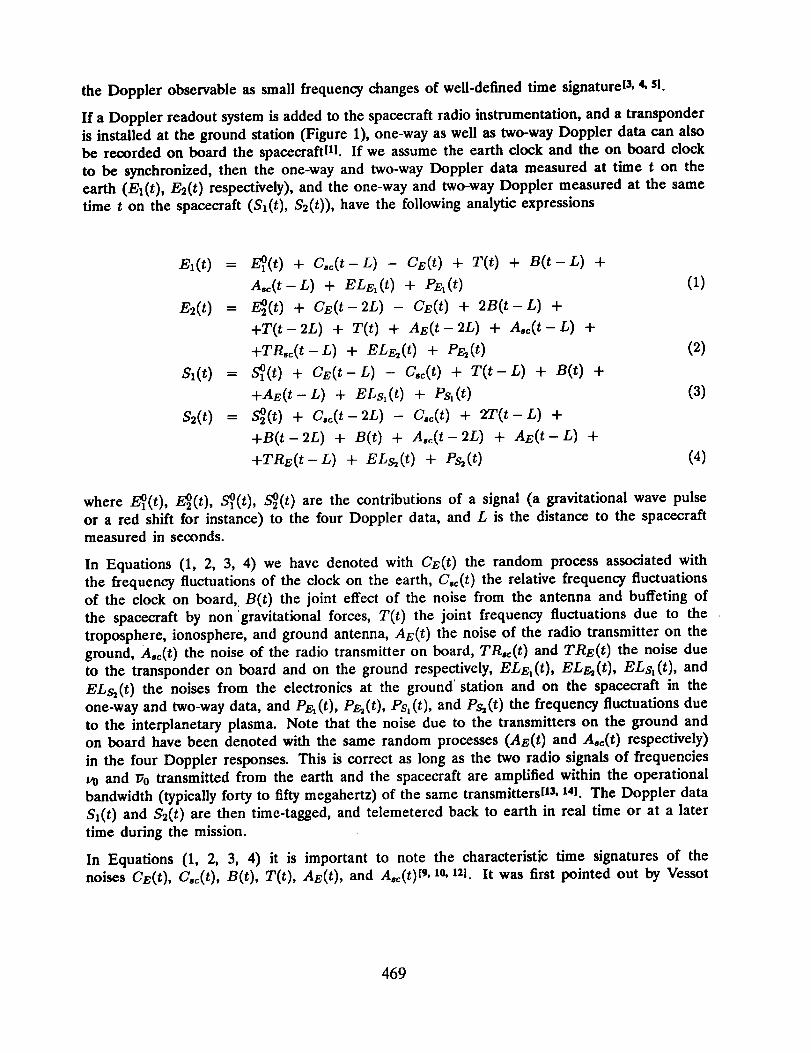
If a Doppler readout system is added to the spacecraft radio instrumentation, and a transponder

is installed at the ground station (Figure 1), one-way as well as two-way Doppler data can also

be recorded on board the spacecraft[ 11. If we assume the earth clock and the on board clock

to be synchronized, then the one-way and two-way Doppler data measured at time t on the

earth (El(t), g2(t) respectively), and the one-way and two-way Doppler measured at the same

time t on the spacecraft (Sl(t), S2(t)), have the following analytic expressions

El(t) = E_l(t) + Coo(t-L) - Cz(t) + T(t) + B(t-L) +

A_(t-L) + ELEa(t) + PEa(t) (1)

E2(t) = E_2(t) + CE(t-2L) - GE(t) + 2B(t-L) +

+T(t-2L) + T(t) + AE(t-2L) + A,,(t-L) +

+TR_(t-L) + ELEa(t) + P_(t) (2)

S,(t) = S_l(t ) + GE(t-L) - Csc(t) + T(t-L) + B(t) +

+AE(t-L) + ELsI(t) + Psi(t) (3)

S2(t) = _(t) + Co,(t-2L) - Cse(t) + 2rF(t - L) +

+B(t-2L) + B(t) + A,c(t-2L) + AE(t--L) +

+TRE(t-L) + EL&(t) + P&(t) (4)

where '_l(t), B_2(t ), S'_l(t), S_2(t) are the contributions of a signal (a gravitational wave pulse

or a red shift for instance) to the four Doppler data, and L is the distance to the spacecraftmeasured in seconds.

In Equations (1, 2, 3, 4) we have denoted with CE(t) the random process associated with

the frequency fluctuations of the clock on the earth, Csc(t) the relative frequency fluctuations

of the clock on board, B(t) the joint effect of the noise from the antenna and buffeting of

the spacecraft by non gravitational forces, T(t) the joint frequency fluctuations due to the

troposphere, ionosphere, and ground antenna, AE(t) the noise of the radio transmitter on the

ground, Asc(t) the noise of the radio transmitter on board, TRy(t) and TRE(t) the noise due

to the transponder on board and on the ground respectively, ELE_(t), ELf(t), ELse(t), and

EL&(t) the noises from the electronics at the ground' station and on the spacecraft in the

one-way and two-way data, and PEa(t), P_(t), Psi(t), and Psi(t) the frequency fluctuations due

to the interplanetary plasma. Note that the noise due to the transmitters on the ground andon board have been denoted with the same random processes (A_(t) and A,,(t) respectively)

in the four Doppler responses. This is correct as long as the two radio signals of frequencies

v0 and _0 transmitted from the earth and the spacecraft are amplified within the operational

bandwidth (typically forty to fifty megahertz) of the same transmittersIl_, 141. The Doppler data

Sl(t) and 52(0 are then time-tagged, and telemetered back to earth in real time or at a later

time during the mission.

In Equations (1, 2, 3, 4) it is important to note the characteristic time signatures of the

noises CE(t), Uo_(t), B(t), T(t), AE(t), and A,c(t)[ 9, 10, 121. It was first pointed out by Vessot

469

and Levinetll that, by properly combining some of the four Doppler data, it was possible to

calibrate the frequency fluctuations of the troposphere, ionosphere, and ground antenna noise,

T(t). Their pioneering work, however, left open the question on whether their existed some

other, perhaps more complicated, linear combinations of the data that would further improve

the sensitivity of Doppler tracking. In what follows we answer this question, and derive a

method that allows us to uniquely identify an optimal way of combining the data.

Let El(f) be the Fourier transform of the time series El(t)

- CEl(f)- E](t) e2"if' dt , (5)O0

and similarly let us denote by E2(f), S](f), S2(f) the Fourier transforms of E,z(t), Sl(t), and

S2(t) respectively. The most general linear combination of the four Doppler data given in Eqs.

(1, 2, 3, 4), can be written in the Fourier domain as follows:

_(f) -- a(f,L) El(f) + b(f,L) E2(f) + c(f,L) Sl(f) + d(f,L) S2(f) (6)

where the coefficients ¢, b, c, d are for the moment arbitrary functions of f and L. If we

substitute in Equation (6) the Fourier transforms of Eqs. (1, 2, 3, 4) we deduce the followingexpression

_(f) [a _l(f! -t-b _22(f) -I-c _11(f)+ d _22(f)]+

+C'-'EE(f) [-- a + b (e 't_rifL - 1) + c e2'xi'fL] "_"

"l"_(f) [_ e 21vi_fL -- C "l" d (e41./'fL-- 1)] -t-

+_(:) [a + b(_,,_IL+1) + _:"_" + _d:'_I"]-_-B(f) [a, e 21"/'fL "1- 2b e 2_/'fL + C -t- d (e4¢/'t'L4- 1)]

+A-_(:)[b_/" + _:-'-- + d,_"/_]++A.'-_cCf)[ae 2"till + be 2'rUL + d eOrilL] +

++

+

+

+ b[TRsc(f)e 2"ffL + E"_z_(f) + P"_(f)]

+ d[T'RE(f)e 2_/L + EL""_(f)+ P"_(,f)]

+

(_)

The four coefficients a, b, c, d, can be determined by requiting the transfer functions of therandom processes _E(f), Co"_c(f), T(f), B(f), "A'EE(f),A_(f) in Equation (7) to be simultaneously

equal to zero, and by further checking that this solution gives a non-zero signal in the

corresponding combined data. This condition implies that a_ b, c, d must satisfy a homogeneous

linear system of six equations in four unknowns. We calculated the rank of the (6 × 4) matrix

associated with this linear system by using the algebraic computer language Mathematica, and

470

we found it to be equal to two. The corresponding solution can be written in the following

way

a(f,L) = c(f,L)e -2_/z - d(f,L) [e2_]L _ e-2_IL]

b(f, L) = - c(f, L) _ -2_i1L -- d(f, L) e-2"_IL , (8)

where e and d can be any arbitrary complex functions not simultaneously equal to zero. After

substituting Equation (8) into Equation (7), we have derived the expressions for the signal

in the case of a gravitational wave pulse or in the variation of the gravitational potential as

experienced by a spacecraft orbiting a celestial body (redshift measurements). We found that

for both these signals their combined Doppler responses (Equation (7)) also vanish. These

results imply that, at any Fourier frequency f and for these two specific Doppler experiments,we can remove only one of the considered noise sources. Among all the noise sources affecting

spacecraft Doppler tracking, the frequency fluctuations due to the troposphere, ionosphere, andmechanical vibrations of the ground antenna, T(f), are the largest. We can choose a, b, c, d

in such a way that the transfer function of T(f) in the combined data is equal to zero. From

Equation (7) we find that a, b, c, d, must satisfy the following equation

a(f,L) =- b(f,L) [e4"ifL + 1]- c(f,L) e2'dIL - 2d(f,L) e2"_IL • (9)

Since b, c., d can not be equal to zero simultaneously, we will choose c to be equal to 1/2, and

b, d to be equal to zero. In other words we will consider only linear combinations of one-way

Doppler data. Note that with this choice we eliminate from y(t) the frequency fluctuations due

to the transponders and the interplanetary plasma affecting the two-way Doppler data. These

considerations imply the following expression for _'(f)

_'(f) = _ -

,2.,,,. ++ 20o)

Equation (10) shows that the transfer functions of the noise of the on board clock, O,c(/),

and of buffeting/3(f), can in principle be set to zero (not simultaneously) at specific Fourier

frequencies. In searches for gravitational wave pulses it has been shown[ 21 that one can reduce

by several orders of magnitudes the noise of the on-board clock at the nulls of its transferfunction without removing the gravitational wave signal. For redshift experiments instead, acancellation of the noise of the on-board clock at those frequencies removes also the signal.

If, however, measurements of y(t) are made at the Fourier frequencies for which the transfer

function of/_(f) is equal to zero, some further improvement in sensitivity can be achievedtlSl.

471

EXPECTED XYLOPHONE SENSITIVITIES

In what follows we provide the expression for the noise in y(t) at the xylophone frequencies

in the case of gravitational wave searches. The analogous expression for redshift experiments

can easily be derived in similar fashion.

Let d_ be the time interval over which a Doppler tracking search for gravitational waves

is performed. The corresponding frequency resolution Af of the data is equal to 1/& This

implies that the fluctuations of the clock on board can be minimized at the following frequencies

fk = (2k- I) -4- A--L • k : 1,2,3, .... (11)4L 2 '

At these frequencies, and to first order in Af L, the Doppler response _(fk) is equal to

1 [_.ol(fk)+ i (_l)k E'_?l(_k)] + i(-1) k+l _(./ek) + 0rihf L) C"se(fk) +3

1 - '÷1] ++B(A) + 3

+2 -- P_(fk) (-1)k+1] +

1 ++3 (12)

For a typical gravitational wave experiment, 6 = 40 days, and Af = 3.0 x 10 -7. Therefore, the

frequency fluctuations of a clock on board a spacecraft that is out to 1 AU are reduced at the

xylophone frequencies by the following amount:

_rAfL = 4.7 x 10 -4 .c

We should point out, however, that these resonant frequencies in general will not be constant,

since the distance to the spacecraft will change over a time interval of forty days. As an

example, however, let us assume again L = 1 AU, 6 = 40 days, and f = 5 x 10 -4 Hz. The

variation in spacecraft distance corresponding to a frequency change equal to the resolution bin

width (3 x 10 -7 Hz) is equal to 1.0 × 105 Kin. Trajectory configurations fulfilling a requirement

compatible to the one just derived have been observed during past spacecraft missions[91, and

therefore we do not expect this to be a limiting factor.

From Equation (12) we can estimate the expected root-mean-squared (r.m.s.) noise level a(fk)

of the frequency fluctuations in the bins of width A.t', around the frequencies fk (k = 1, 2, 3, .... ).

This is given by the following expression

a(fk) = [Sy(fk) Af] 1/2 , k = 1,2,3, ..... (13)

472

where S_(f_) is the one-sided power spectral density of the noise sources in the Doppler response

y(t) at the frequency fk. In what follows we will assume that the random processes representingthese noises are uncorrelated with each other, and their one-sided power spectral densities are

as given in Table I. In this table we have assumed a frequency stability of 1.0 × 10 -16 at 1000

seconds integration time for the clock at the ground station. Although this is a factor of fourbetter than what has been measured so far[Ill, it seems very likely that by the beginning of

next century such a sensitivity can be achieved. As far as the other sensiti_ty figures provided

in Table I are concerned, they are as given in the Riley et al. report[ ul. This document is

a summary of a detailed study, performed jointly by scientists and engineers of NAS,_s Jet

Propulsion Laboratory .and the Italian Space Agency (ASI) Alenia Spazio, for assessing the

magnitude and spectral characteristics of the noise sources that will determine the Doppler

sensitivity of the future gravitational wave experiment on the Cassini mission. Included in Table

I is also the spectral density of the noise of a crystal-driven ultra-stable oscillator (USO).

If dual radio frequencies in the uplink and downlink are used, then the frequency fluctuations

due to the interplanetary plasma can be entirely removed [nl. We will refer to this configuration

as MODE I. If only one frequency is adopted instead, which we will assume to be Ka-Band

(32 GHz), we will refer to this configuration as MODE II. Ka-Band is planned to be used onmost of the forthcoming NASA missions, and will be implemented on the ground antennas of

the Deep Space Network (DSN) by the year 1999 for the Cassini mission.

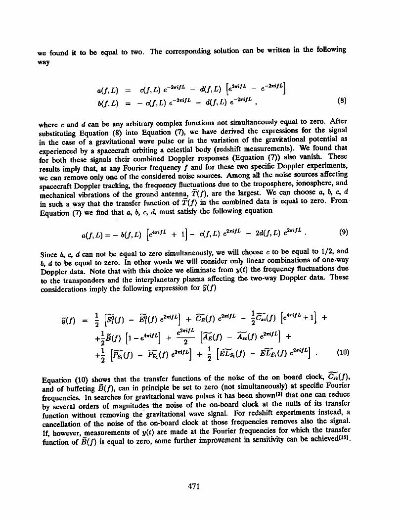
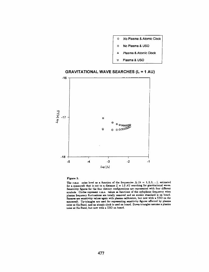
In Figure 2 wc plot the r.m.s, a(fk) of the noise as a function of the frequencies fk (k =

1, 2, 3, .... ), assuming that an interplanetary spacecraft is out to a distance L = 1.0 AU. For this

configuration the fundamental frequency of the xylophone (Equation (11)) is equal to 5.0 x 10-4

Hz. A complete analysis covering configurations with spacecraft at .several other distances is

given in[21.

The MODE I configuration is represented by two curves, depending on whether an atomic clock

(circles) or a USO (squares) is operated on board the spacecraft. Sensitivity curves for the

MODE II configuration are also provided, again with an atomic clock on board (up-triangles)

or a USO (down-triangles). The best sensitivity is achieved in the MODE I configuration,

regardless of whether an atomic clock or a USO is operated on board the spacecraft (circles

and squares are over imposed). This is because the amplitude of the noise of the clock on

board is reduced by a factor lrAfL/c = 4.7 × 10-4 at the xylophone frequencies. At f = 10-3

Hz the corresponding r.m.s, noise level is equal to 4.7 × 10 -is, and it increases to a value of5.7 × 10 -is at f = 10 -2 Hz. As far as the MODE II configuration is concerned, the r.m.s.

noise level is equal to 7.9 x 10 -18 at f = 10 -3 I/z, while it decreases to 6.3 × 10 -Is at f = 10 -2

Hz. This is due to the fact that the one-sided power spectral density of the fractional frequency

fluctuations due to the interplanetary plasma decays as f-21z.

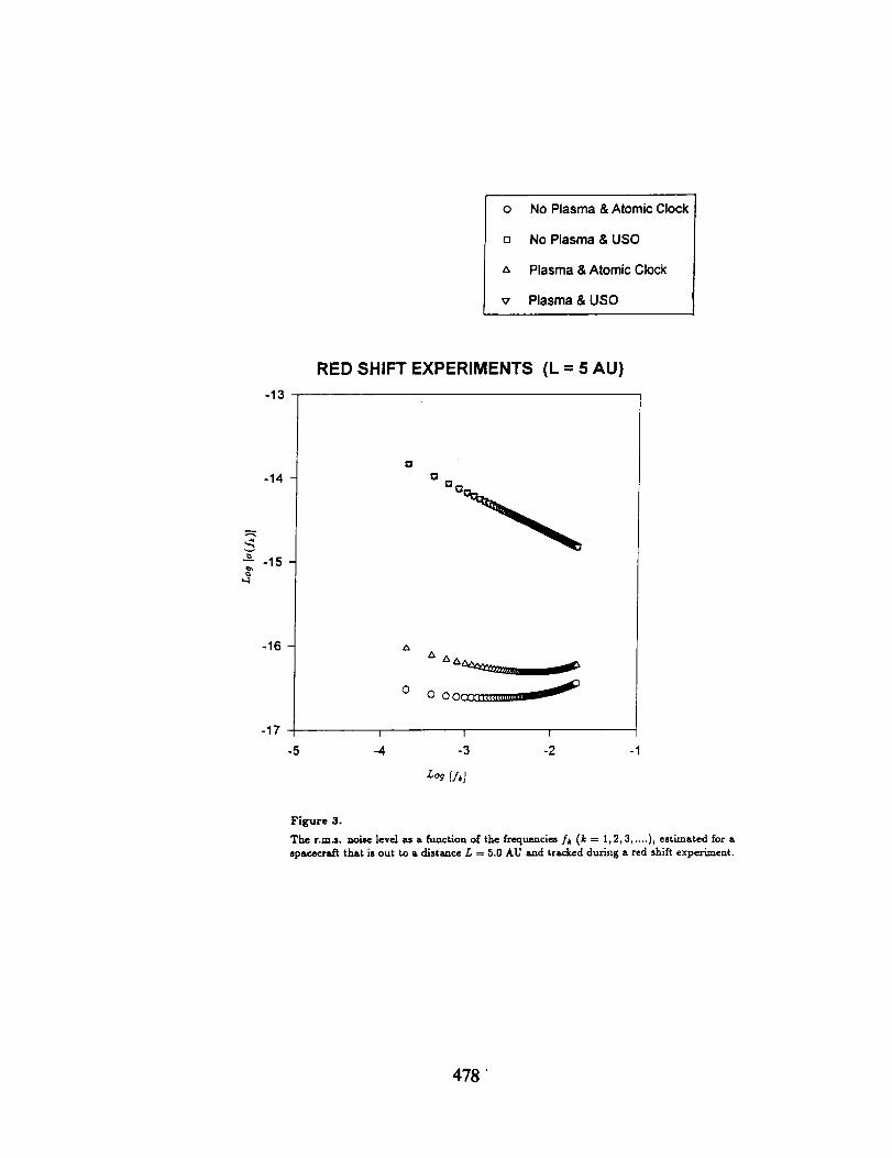
In Figure 3 we turn to redshift experiments with a spacecraft out to 5 AU, and we assume an

observing time of 40 hours. This example can be considered as representative of a spacecraft

orbiting the planet Jupiter. The reduction factor of the buffeting noise B(t) (see Equation

(10)) is now equal to

lrAfL = 5.5 × 10 -2 , (14)C

473

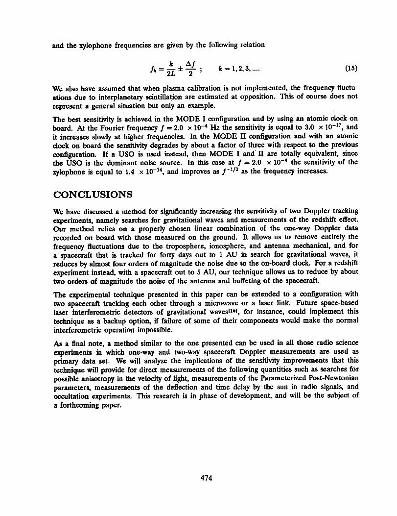
and the xylophone frequencies are given by the following relation

k a/fk----:-_-. +-:- ; k----1,2,3, .... (15)

We also have assumed that when plasma calibration is not implemented, the frequency fluctu-

ations due to interplanetary scintillation are estimated at opposition. This of course does not

represent a general situation but only an example.

The best sensitivity is achieved in the MODE I configuration and by using an atomic clock on

board. At the Fourier frequency f = 2.0 x 10 --4 Hz the sensitivity is equal to 3.0 x 10 -17, and

it increases slowly at higher frequencies. In the MODE II configuration and with an atomic

clock on board the sensitivity degrades by about a factor of three with respect to the previous

configuration. If a USO is used instead, then MODE I and" II are totally equivalent, sincethe USO is the dominant noise source. In this case at f = 2.0 x 10 -4 the sensitivity of the

xylophone is equal to 1.4 x 10 -14, and improves as f-1/2 as the frequency increases.

CONCLUSIONS

We have discussed a method for significantly increasing the sensitivity of two Doppler tracking

experiments, namely searches for gravitational waves and measurements of the redshift effect.

Our method relies on a properly chosen linear combination of the one-way Doppler data

recorded on board with those measured on the ground. It allows us to remove entirely the

frequency fluctuations due to the troposphere, ionosphere, and antenna mechanical, and for

a spacecraft that is tracked for forty days out to 1 AU in search for gravitational waves, it

reduces by almost four orders of magnitude the noise due to the on-board clock. For a redshift

experiment instead, with a spacecraft out to 5 AU, our technique allows us to reduce by about

two orders of magnitude the noise of the antenna and buffeting of the spacecraft.

The experimental technique presented in this paper can be extended to a configuration with

two spacecraft tracking each other through a microwave or a laser link. Future space-based

laser interferometric detectors of gravitational waves[161, for instance, could implement this

technique as a backup option, if failure of some of their components would make the normal

interferometric operation impossible.

As a final note, a method similar to the one presented can be used in all those radio science

experiments in which one-way and two-way spacecraft Doppler measurements are used as

primary data set. We will analyze the implications of the sensitivity improvements that this

technique will provide for direct measurements of the following quantities such as searches for

poss_le anisotropy in the velocity of light, measurements of the Parameterized Post-Newtonian

parameters, measurements of the deflection and time delay by the sun in radio signals, and

occultation experiments. This research is in phase of development, and will be the subject of

a forthcoming paper.

474

REFERENCES

[1] R.EC. Vessot, and M.W. Levine 1979, Gen. Relativ. Gravit., 10, 181.

[2] M. Tinto, Phys. Rev. D, in press.

[3] J.D. Anderson, et al. 1980, Science, 207, 449-453.

[4] J.D. Anderson, et al. 1986, Icarus, 71, 337-349.

[5] F.B. Estabrook, and H.D. Wahlquist 1975, Gen. Rel. Gray., 6, 439.

[6] J.W. Armstrong, R. Woo, and EB. Estabrook 1979, Astrophys. J.,30 574.

[7] I.I. Shapiro, et al 1977, J. Geophys. Res., 82, 4329-4334.

[8] J.D. Anderson, et al. 1978, Astronautica, 5, 43-61.

[9] J.W. Armstrong 1989, in Gravitational Wave Data Analysis, cd. B.E Schutz (Kluwer,

Dordrecht), p. 153.

[10] L.L. Smarr, R.EC. R.EC. Vessot, C.A. Lundquist, R. Dechcr, and T. Piran 1983, Gen.

Relativ. Gravit., 15, 2.

[11] A.L. Riley, D. Antsos, J.W. Armstrong, P. Kinman, H.D. Wahlquist, B. Bcrtotti, (3.

Comoretto, B. Pernice, G. Camicella, and R. Giordani 1990, Jet Propulsion Laboratory

Report, Pasadena, California, 22 January 1990.

[12] T. Piran, E. Reiter, W.G. Unruh, and R.EC. Vessot 1986, Phys. Rev. D, 34, 984.

[13] R. Perez 1989, Jet Propulsion Laboratory, InterOffice Memorandum 3337-89-098, 3 Oc-tober 1989.

[14] B.L. Conroy, and D. and Lee 1990, Rev. Sci. Instrum., 61, 1720.

[15] M. Tinto, unpublished.

[16] LISA: (Laser lnterferometer Space Antenna), Proposal for a Laser-lnterferometrie

Gravitational Wave Detector in Space, 1993, MPQ 177 (Max-Planek-Institute fftr Quan-

tenoptie, Garehing bei Mfmehen).

475

Transponder.,,

l

[

I

I

I

l

U--- l-

l

II

"4" TrlnsmitterChain

DSN

"-_ Receiver Chain II

s/c

[_ ......

H-Maser

&

FrequencyDistribution

. l:T..nd,iI,I

An_p[ificr j

I

, tR_ei_e_Ch_JI II II If I

, I

I (uso) !ySz(t)

Figure 1.

Block diagram of the radio hardware at the ground antenna of the NASA Deep Spac_ Net-work (DSN) _ad on board the spacecra/t(S/C), that aJ.lows the acqu.isitionAnd recordingof the four Doppter data El(t), E_(t), Sl(t), and S_(t).

Error Source

One-Way Plasma

(@ Ka-Band)

H-Ma_er

Frequency Disr_nbudon

Allan Deviation

@ 1,000 sec.

Fractional FrequencyOne-Sided

Power Spectral

Density

4.9 x I0 "1¢ 2.7 x 10 "_ f" _

1.0 x tO"16 6.2 x (10"zsf+ i0 .n ft

+ 10 J° )

1.0 x I0 "_ 1.3 x 10"2_ f:

Receiver chain 3.1 x I0 "_7 1.3 x i0 "'_ f"

Trasmitter chain 3.4 x i0 "L6 2.3 x 10"z'

Thermal Noise 3.8 x I0 "_7 1.9 x 10"u f:

Spacecra& A.me:'ma & 5.8 x 10-.7 5.0 x 10"2 f J + I0 _'

Buffeting +5.0 x I0 "_

Spacecraft _o[ifier 5.0 x I0''7 4.0 x i0 "_ f

9.5 x i0"" 6.5 x 10 .27f "USO

Table I

List of the noiJe sources entering into the combined Doppier response y(t). The .Allandeviation at a given integration time r is a statistical parameter for describing frequency.stability. It represents the root-mean-squared expectation value of the random processmociated withthefi-a.ctionalfrequencychanges,betweentime.contiguou_frequencymea-

surements,each m_de over time interv_ or"duration _'. The numbers provided in thistable are taken from the Riley et al. report {111.

476

o No Plasma & Atomic Clock

[] No Plasma & USO

a Plasma & Atomic Clock

v Plasma & USO

GRAVITATIONAL WAVE SEARCHES (L = 1 AU)

-16

-17 -

-18

-5

=3

=3 O¢

0 0 0 0033_

I I I

-4 -3 -2 -1

Lo9[/_l

Figure 2.

The r.m.s, noise level am a function of the frequencies fk (k = 1,2,3,....), estimated

for a spacecrmet that is out to a dlstance r. _- 1.0 AU searcb.ing for gravitational w_ves.

Semfitivlty f_n_res for the four distinct configurations are represented with four different

symboL. Circles represent r.m.s, values u functions of the xylophone frequency when

plnsraA frequency fluctuations are totally removed and an atomic standard is on ho_zl.

SquLres are semfitivity v_ues again with plasma calibration, but now with a USO on the

spacecraft. Up-triangleJ are roped for representing sensitivity figure_ affected by pl-cmanoise at KL-Band, and an atomic clock is used on board. Down-triangles a._ume a pluma

noise at KA-Band, but now with a USO on board.

477

o No Plasma & Atomic Clock

a No Plasma & USO

z_ Plasma & Atomic Clock

v Plasma&USO

-13

RED SHIFT EXPERIMENTS (L = 5 AU)

-14

-15

-16

-17

Z_

I I I

-5 -4 -3 -2 -"

Zog[A]

Figure 3.

The r.m.s, noise level as a function of the frequencies fk (k = 1,2,3, ....), estimated for a

spacecra/'t that is out to a el[stance L = 5.0 AU and tracked during a red shift expex/ment.

478 '