Sound Modeling: signal-based approaches (part...

Sound Modeling: signal-based approaches (part 2)

Sound Analysis, Synthesis and Processing

Paolo Bestagini

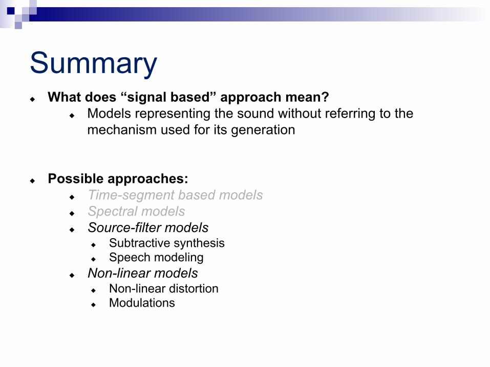
Summary u  What does “signal based” approach mean?

u  Models representing the sound without referring to the mechanism used for its generation

u  Possible approaches: u  Time-segment based models u  Spectral models u  Source-filter models

u  Subtractive synthesis u  Speech modeling

u  Non-linear models u  Non-linear distortion u  Modulations

Source-filter models

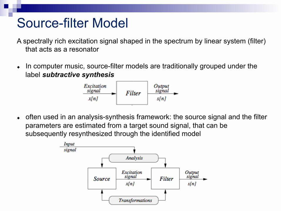
Source-filter Model A spectrally rich excitation signal shaped in the spectrum by linear system (filter)

that acts as a resonator u  In computer music, source-filter models are traditionally grouped under the

label subtractive synthesis

u  often used in an analysis-synthesis framework: the source signal and the filter

parameters are estimated from a target sound signal, that can be subsequently resynthesized through the identified model

Digression: z-transform u  Z-transform and filters:

u  Time domain

u  Z domain

u  Examples:

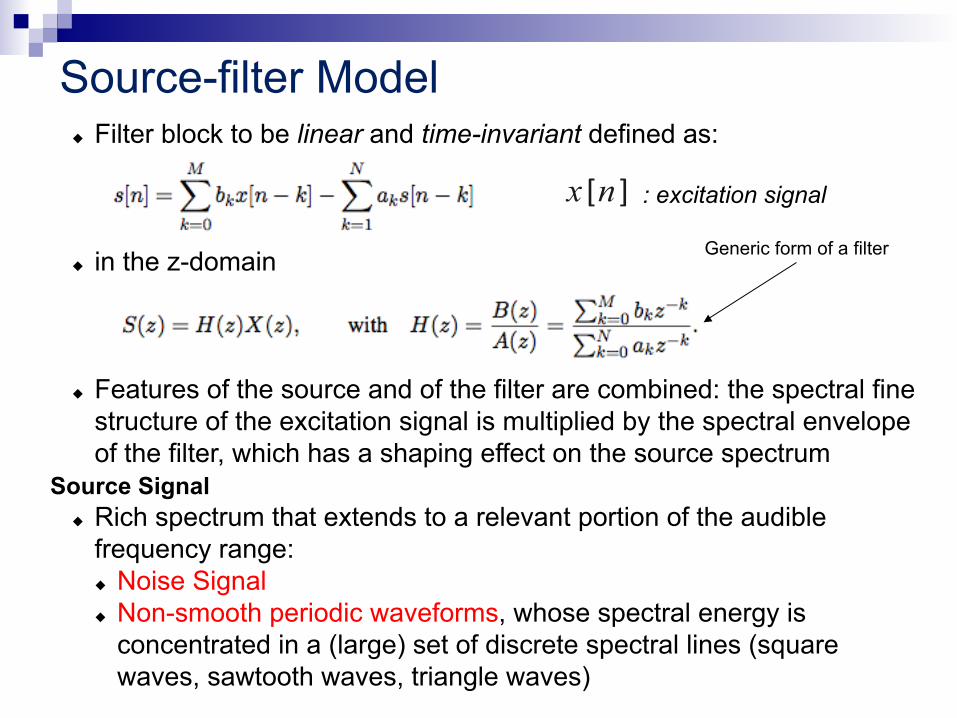
Source-filter Model u  Filter block to be linear and time-invariant defined as:

u  in the z-domain

u  Features of the source and of the filter are combined: the spectral fine structure of the excitation signal is multiplied by the spectral envelope of the filter, which has a shaping effect on the source spectrum

u  Rich spectrum that extends to a relevant portion of the audible

frequency range: u  Noise Signal u  Non-smooth periodic waveforms, whose spectral energy is

concentrated in a (large) set of discrete spectral lines (square waves, sawtooth waves, triangle waves)

: excitation signal

Source Signal

Generic form of a filter

x [n ]

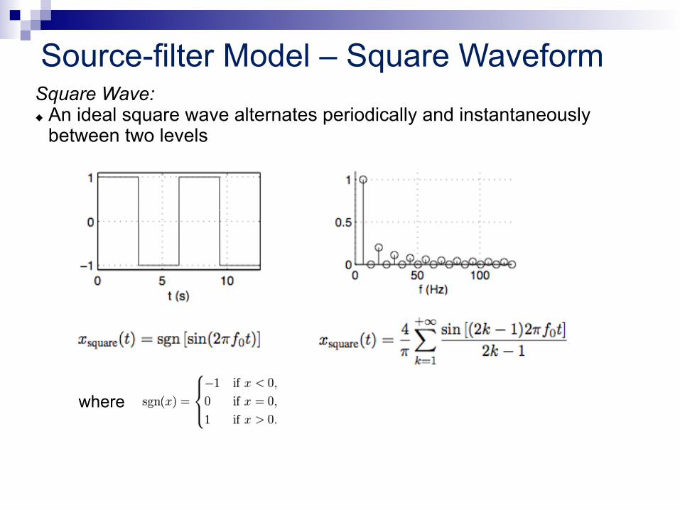
Source-filter Model – Square Waveform Square Wave: u  An ideal square wave alternates periodically and instantaneously

between two levels

where

Source-filter Model – Square Waveform Triangular Wave u An ideal triangular wave alternates periodically between a linearly rising portion and a linearly decreasing portion

Source-filter Model – Square Waveform Sawtooth Wave u An ideal sawtooth wave is a periodic series of linear ramps

where is the floor function.

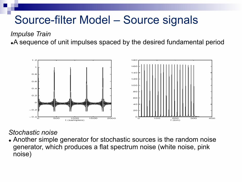
Source-filter Model – Source signals Impulse Train u A sequence of unit impulses spaced by the desired fundamental period

Stochastic noise u  Another simple generator for stochastic sources is the random noise

generator, which produces a flat spectrum noise (white noise, pink noise)

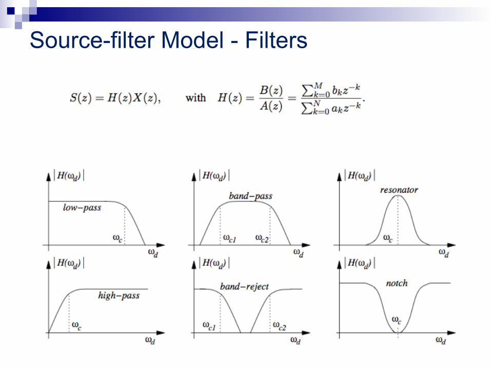
Source-filter Model - Filters

Source-filter Model – Filters Resonant Filter l The second-order IIR filter is the simplest one, and is described by a transfer function l where r and ±ωc are the magnitude and phases of the poles, and the condition r < 1 must hold in order for the filter to be stable

Source-filter Model – Speech Modeling

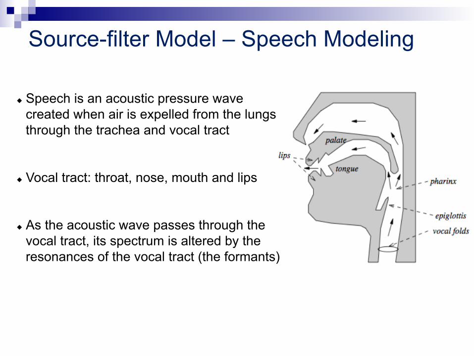
u  Speech is an acoustic pressure wave created when air is expelled from the lungs through the trachea and vocal tract

u  Vocal tract: throat, nose, mouth and lips u  As the acoustic wave passes through the

vocal tract, its spectrum is altered by the resonances of the vocal tract (the formants)


u  Voiced sounds (vowels or nasals): result from a quasi-periodic excitation of the vocal tract caused by

oscillation of the vocal folds in a quasi-periodic fashion u  Unvoiced sounds: do not involve vocal fold oscillations and are typically associated to

turbulent flow generated when air passes through narrow restrictions of the vocal tract

u  During voiced signals:

u  the quasi-periodic nature of the oscillations gives rise to an harmonic signal

u  the frequency associated with the first harmonic partial is commonly termed the pitch of the voiced signal


u Concatenative synthesis u  Connect pre-recorded natural phonetic units

u  Pros: Easiest way and the most popular approach to produce intelligible and natural sounding synthetic speech

u  Cons: Are usually limited to one speaker and one voice and usually require much memory – Not flexible

u Formant Synthesis u  Formant synthesis is based on the source-filter modeling approach

Source: acoustic flow Filter: vocal tract

u  The transfer function of the vocal tract is typically represented as a series of resonant filters, each accounting for one formant

u Articulatory synthesis u  Model the human speech production system directly u  Parameters associated to vocal folds: glottal aperture, fold tension,

lung pressure, etc. u  Pros: promise high quality synthesis u  Cons: computational costs are high, parametric control is arduous


Formant Synthesis u  Formant synthesis of speech realizes a source-filter model:

u  a broadband source signal undergoes multiple filtering transformations that are associated to the action of different elements of the phonatory system

u  If s[n] is a voiced speech signal, it can be expressed in the z-domain as:

u  the source signal X(z) is a periodic pulse train whose period coincides with the pitch of the signal and gv is a constant gain term

u  G(z) is a filter associated to the response of the glottis (the vocal folds) to pitch pulses

u  V (z) is the vocal tract filter u  R(z) simulates the radiation effect of the lips

u  If s[n] is a unvoiced speech signal

u  The turbulence can be modeled as white noise, so X(z) is a white noise sequence


Formant Synthesis G(z) shapes the glottal pulses

u  since the input x[n] is a pulse train, the output is the impulse response g[n] of this filter

u  A model is a IIR low pass filter


Vi ( z)

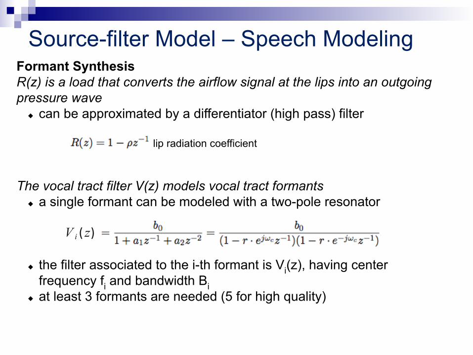
Formant Synthesis R(z) is a load that converts the airflow signal at the lips into an outgoing pressure wave

u  can be approximated by a differentiator (high pass) filter

where ρ is a lip radiation coefficient The vocal tract filter V(z) models vocal tract formants

u  a single formant can be modeled with a two-pole resonator

u  the filter associated to the i-th formant is Vi(z), having center frequency fi and bandwidth Bi

u  at least 3 formants are needed (5 for high quality)


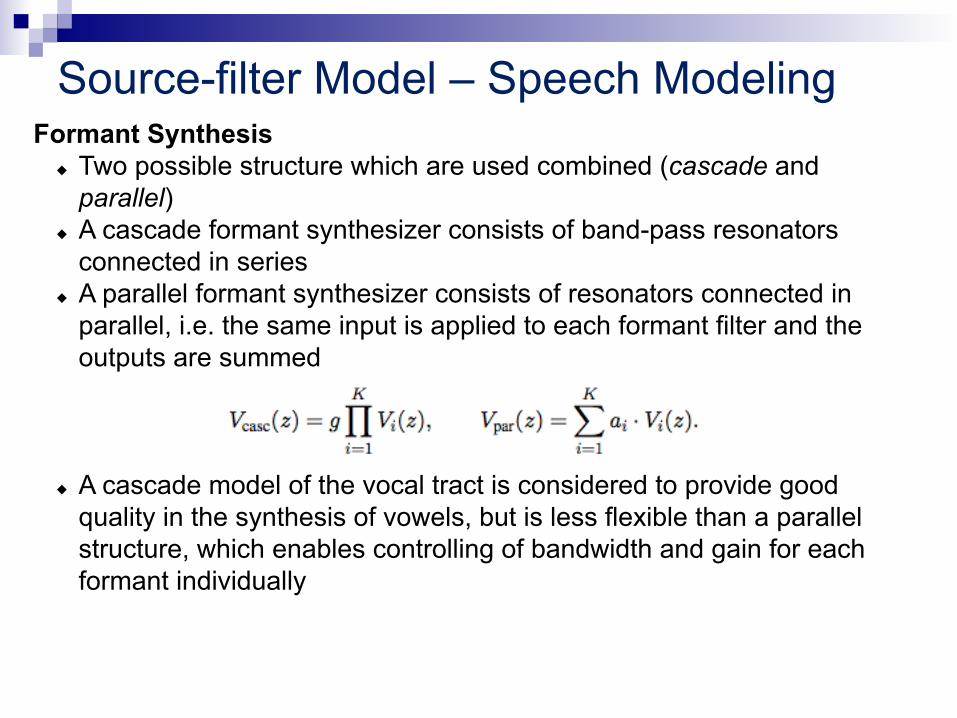
Formant Synthesis u  Two possible structure which are used combined (cascade and

parallel) u  A cascade formant synthesizer consists of band-pass resonators

connected in series u  A parallel formant synthesizer consists of resonators connected in

parallel, i.e. the same input is applied to each formant filter and the outputs are summed

u  A cascade model of the vocal tract is considered to provide good

quality in the synthesis of vowels, but is less flexible than a parallel structure, which enables controlling of bandwidth and gain for each formant individually


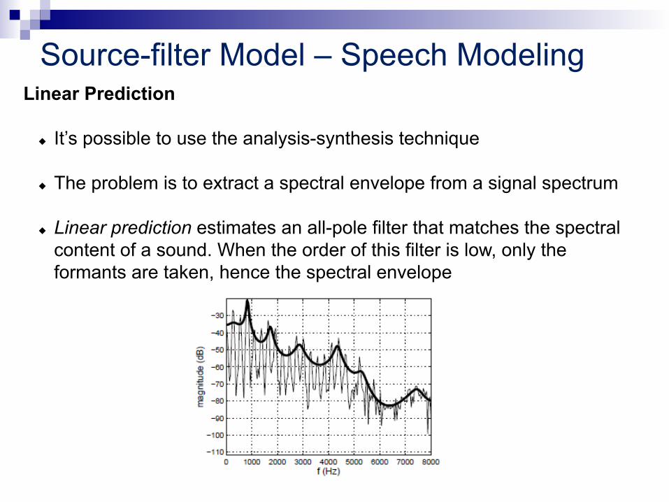
Linear Prediction

u  It’s possible to use the analysis-synthesis technique u  The problem is to extract a spectral envelope from a signal spectrum u  Linear prediction estimates an all-pole filter that matches the spectral

content of a sound. When the order of this filter is low, only the formants are taken, hence the spectral envelope

Source-filter Model – Speech Modeling Example: •  The frequencies of the source and the frequencies of the filter are independent •  This is why it is sometimes difficult to understand the vowels of a soprano

singing at the top of her range.

Non linear models

Non linear Models u  The transformations seen until now are linear (a):

u  frequency does not change u  Using non linear (b) transformations:

u  frequencies can be drastically changed u  new components are created

It is possible to vary substantially the nature of the input sound

Non linear Models

u  Two main effects: u  Spectrum enrichment:

u  due to non linear distortion u  allows for controlling the brightness of a sound

u  nonlinearities and saturations found on real systems e.g. analog amplifiers, electronic valves

u  Spectrum shift:

u  due to multiplication of the signal by a sinusoid u  moves the spectrum, altering the harmonic relationship between the

modulating signal lines u  used in electronic music and it is a new metaphor for computer

musicians

Non linear Models – Non linear distortion (Waveshaping)

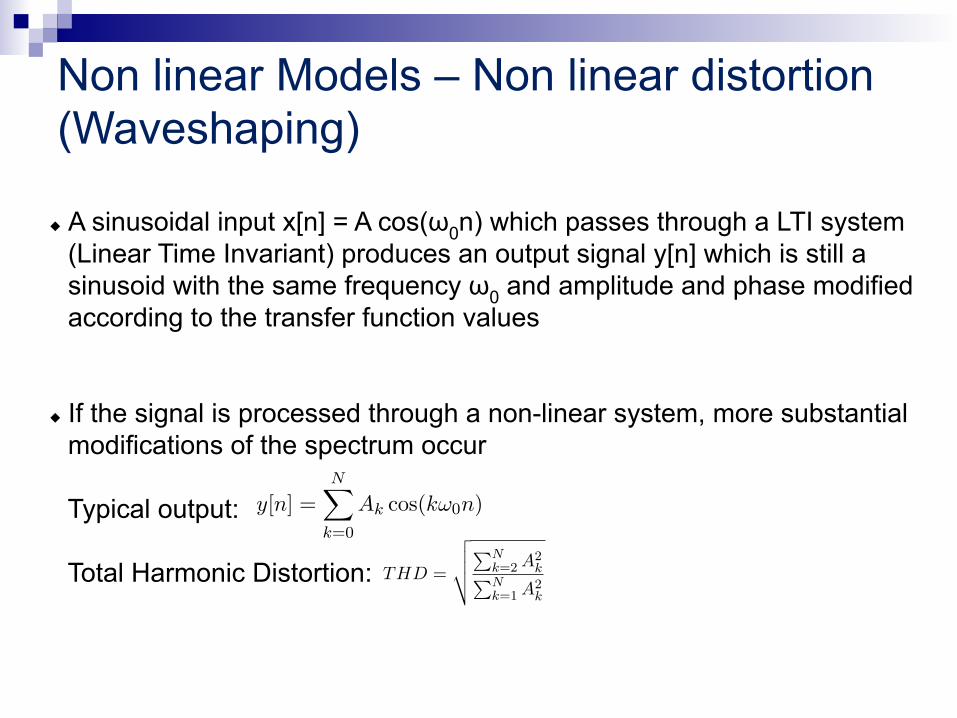
u  A sinusoidal input x[n] = A cos(ω0n) which passes through a LTI system

(Linear Time Invariant) produces an output signal y[n] which is still a sinusoid with the same frequency ω0 and amplitude and phase modified according to the transfer function values

u  If the signal is processed through a non-linear system, more substantial

modifications of the spectrum occur Typical output:

Total Harmonic Distortion:

Chapter 2. Sound modeling: signal-based approaches 2-45

0 1 2 3 4 5 6x 10−3

−1

−0.5

0

0.5

1

t (s)

(a)

0 1 2 3 4 5 6x 10−3

−1

−0.5

0

0.5

1

t (s)

(b)

Figure 2.26: Example of output signals from a linear and from a non-linear system, in response to asinusoidal input; (a) in a linear system the input and output differ in amplitude and phase only; (b) ina non-linear system they have different spectra.

trum to the vicinity of the carrier signal, altering the harmonic relationship between the modulatingsignal lines. The possibility of shifting the spectrum is very intriguing in when applied to music.From simple components, harmonic and inharmonic sounds can be created, and various harmonicrelations among the partials can be established. The first effect try to reproduce the nonlinearities andsaturations found on real systems e.g. analog amplifiers, electronic valves. The second one insteadderives from abstract mathematical properties of trigonometric functions as used in modulation theoryapplied to music signal. Therefore, it inherits, in part, the analogic interpretation as used in electronicmusic and is a new metaphor for computer musicians.

2.6.1 Memoryless non-linear processing

2.6.1.1 Harmonic distortion and waveshaping

In Chapter Fundamentals of digital audio processing we have seen that a sinusoidal input x[n] = A cos(ω0n)

which passes through a LTI system (a filter) produces an output signal y[n] which is still a sinusoidwith the same frequency ω0 and amplitude and phase modified according to the transfer functionvalues (see Fig. 2.26(a)). On the other hand, if the signal is processed through a non-linear system,more substantial modifications of the spectrum occur: the output has in general the form

y[n] =

NX

k=0

Ak

cos(kω0n), (2.49)

and therefore the spectrum of y possesses energy at higher harmonics of ω0 (see Fig. 2.26(b)). Thiseffect, which is characteristic of non-linear systems, is termed harmonic distortion, and can be quan-tified through the total harmonic distortion (THD) parameter:

THD =

vuutP

N

k=2 A2kP

N

k=1 A2k

. (2.50)

In many cases one wants to minimize harmonic distortion in non-linear processing, but in other casesdistortion is exactly what we want in order to enrich an input sound. an example is the effect of valves,

This book is licensed under the CreativeCommons Attribution-NonCommercial-ShareAlike 3.0 license,c�2005-2008 by the authors except for paragraphs labeled as adapted from <reference>

Chapter 2. Sound modeling: signal-based approaches 2-45

0 1 2 3 4 5 6x 10−3

−1

−0.5

0

0.5

1

t (s)

(a)

0 1 2 3 4 5 6x 10−3

−1

−0.5

0

0.5

1

t (s)

(b)

Figure 2.26: Example of output signals from a linear and from a non-linear system, in response to asinusoidal input; (a) in a linear system the input and output differ in amplitude and phase only; (b) ina non-linear system they have different spectra.

trum to the vicinity of the carrier signal, altering the harmonic relationship between the modulatingsignal lines. The possibility of shifting the spectrum is very intriguing in when applied to music.From simple components, harmonic and inharmonic sounds can be created, and various harmonicrelations among the partials can be established. The first effect try to reproduce the nonlinearities andsaturations found on real systems e.g. analog amplifiers, electronic valves. The second one insteadderives from abstract mathematical properties of trigonometric functions as used in modulation theoryapplied to music signal. Therefore, it inherits, in part, the analogic interpretation as used in electronicmusic and is a new metaphor for computer musicians.

2.6.1 Memoryless non-linear processing

2.6.1.1 Harmonic distortion and waveshaping

In Chapter Fundamentals of digital audio processing we have seen that a sinusoidal input x[n] = A cos(ω0n)

which passes through a LTI system (a filter) produces an output signal y[n] which is still a sinusoidwith the same frequency ω0 and amplitude and phase modified according to the transfer functionvalues (see Fig. 2.26(a)). On the other hand, if the signal is processed through a non-linear system,more substantial modifications of the spectrum occur: the output has in general the form

y[n] =

NX

k=0

Ak

cos(kω0n), (2.49)

and therefore the spectrum of y possesses energy at higher harmonics of ω0 (see Fig. 2.26(b)). Thiseffect, which is characteristic of non-linear systems, is termed harmonic distortion, and can be quan-tified through the total harmonic distortion (THD) parameter:

THD =

vuutP

N

k=2 A2kP

N

k=1 A2k

. (2.50)

In many cases one wants to minimize harmonic distortion in non-linear processing, but in other casesdistortion is exactly what we want in order to enrich an input sound. an example is the effect of valves,

This book is licensed under the CreativeCommons Attribution-NonCommercial-ShareAlike 3.0 license,c�2005-2008 by the authors except for paragraphs labeled as adapted from <reference>


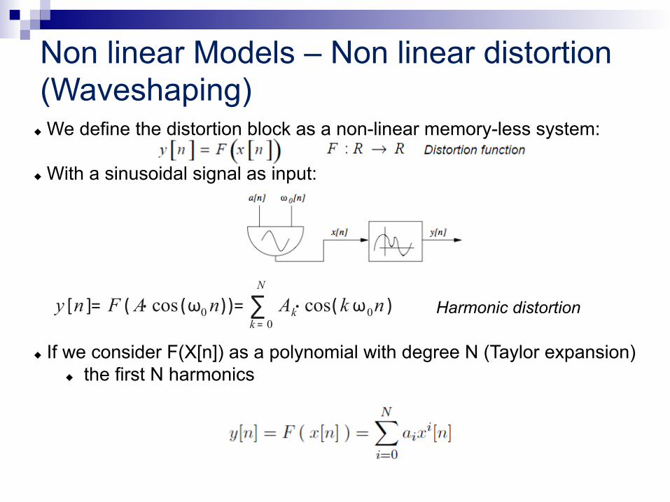
u  We define the distortion block as a non-linear memory-less system: u  With a sinusoidal signal as input: u  If we consider F(X[n]) as a polynomial with degree N (Taylor expansion)

u  the first N harmonics

y [n ]= F ( A⋅ cos (ω0n))= ∑k = 0

N

Ak⋅ cos(kω0n ) Harmonic distortion


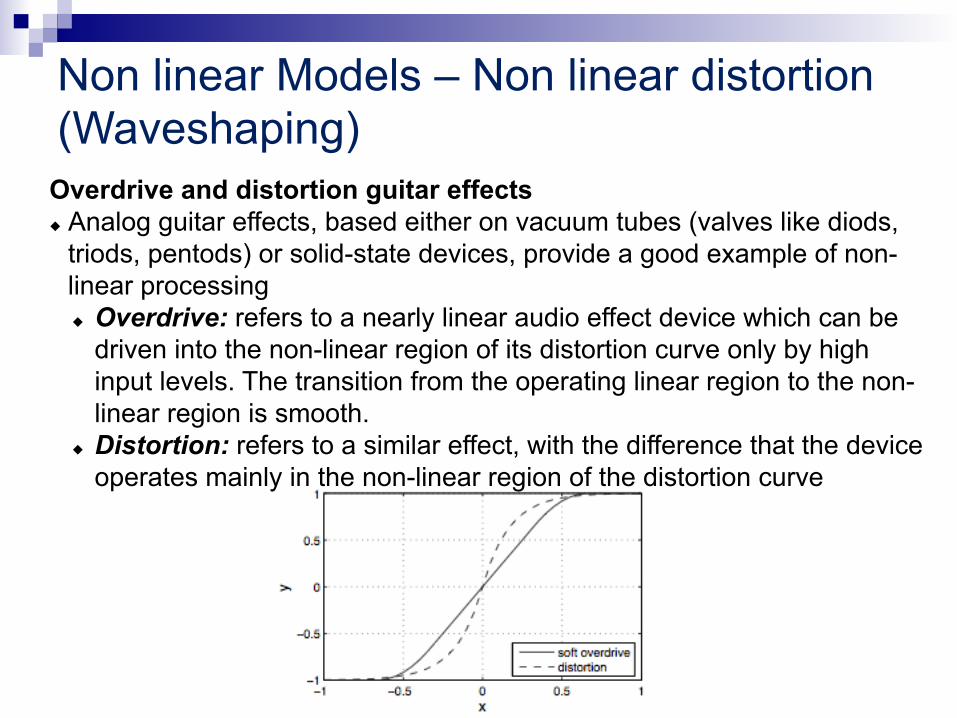
Overdrive and distortion guitar effects u  Analog guitar effects, based either on vacuum tubes (valves like diods,

triods, pentods) or solid-state devices, provide a good example of non-linear processing u  Overdrive: refers to a nearly linear audio effect device which can be

driven into the non-linear region of its distortion curve only by high input levels. The transition from the operating linear region to the non-linear region is smooth.

u  Distortion: refers to a similar effect, with the difference that the device operates mainly in the non-linear region of the distortion curve


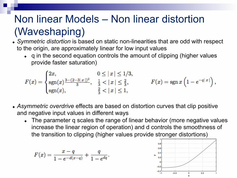
u  Symmetric distortion is based on static non-linearities that are odd with respect to the origin, are approximately linear for low input values

u  q in the second equation controls the amount of clipping (higher values provide faster saturation)

u  Asymmetric overdrive effects are based on distortion curves that clip positive and negative input values in different ways

u  The parameter q scales the range of linear behavior (more negative values increase the linear region of operation) and d controls the smoothness of the transition to clipping (higher values provide stronger distortions)

Non linear Models – Multiplicative Synthesis u  It is most simple technique for spectrum shift and in analog domain it’s called Ring

Modulation (RM) u  Let x1[n] and x2[n] be two input signals u  The spectrum is convolution u  Carrier Signal c[n] is a sinusoid with frequency ωc u  Modulation Signal the second signal is the input that will be transformed by the

ring modulation and is called the modulating signal m[n] u  The Spectrum is u  i.e. S(ωd) is composed of two copies of the spectrum of M(ωd), symmetric around ωc: a lower sideband (LSB), reversed in frequency, and an upper sideband (USB)

s [n]= x1[n]⋅ x2[n ]S (ωd)= [X 1∗ X 2](ωd)

x1[n]= c1[n]= cos(ωcn+ ϕc) x2[n ]= m[n]

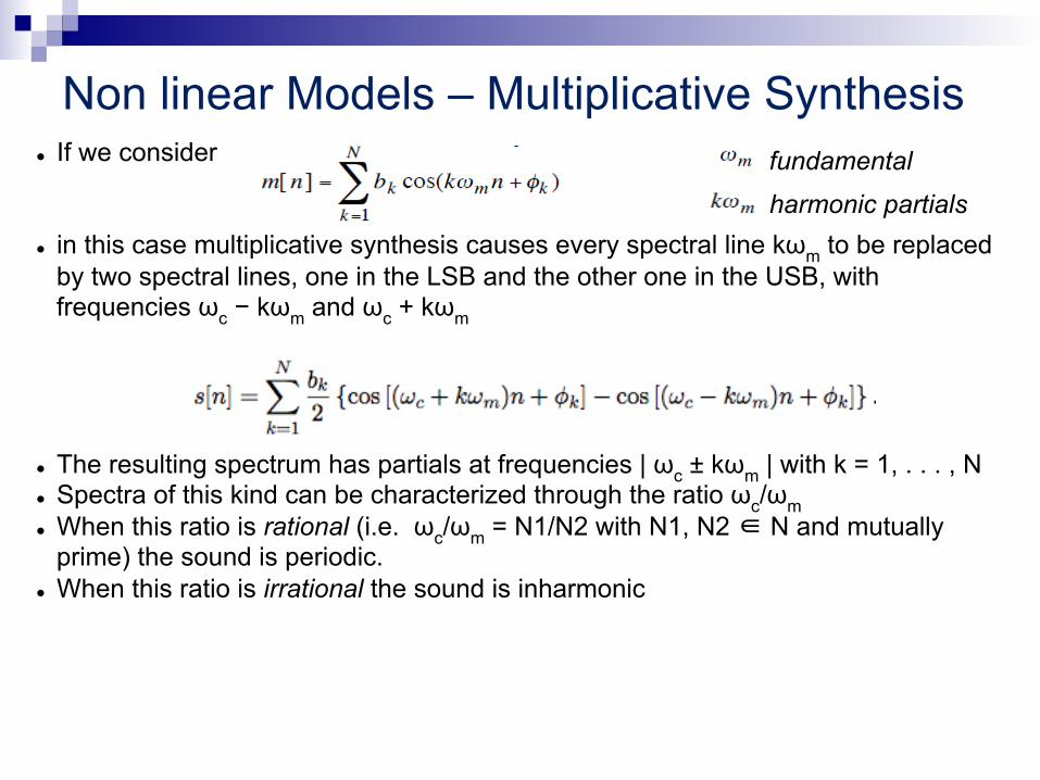
Non linear Models – Multiplicative Synthesis l  If we consider l  in this case multiplicative synthesis causes every spectral line kωm to be replaced

by two spectral lines, one in the LSB and the other one in the USB, with frequencies ωc − kωm and ωc + kωm

l  The resulting spectrum has partials at frequencies | ωc ± kωm | with k = 1, . . . , N l  Spectra of this kind can be characterized through the ratio ωc/ωm l  When this ratio is rational (i.e. ωc/ωm = N1/N2 with N1, N2 ∈ N and mutually

prime) the sound is periodic. l  When this ratio is irrational the sound is inharmonic

fundamental

harmonic partials

Non linear Models – Multiplicative Synthesis – Amplitude Modulation

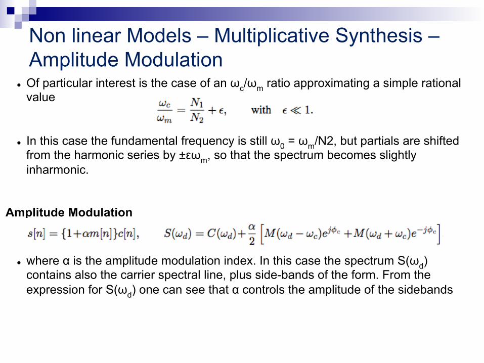
l  Of particular interest is the case of an ωc/ωm ratio approximating a simple rational value

l  In this case the fundamental frequency is still ω0 = ωm/N2, but partials are shifted

from the harmonic series by ±εωm, so that the spectrum becomes slightly inharmonic.

l  where α is the amplitude modulation index. In this case the spectrum S(ωd) contains also the carrier spectral line, plus side-bands of the form. From the expression for S(ωd) one can see that α controls the amplitude of the sidebands

Amplitude Modulation

Non linear Models – Frequency Modulation l Frequency modulation l They are not derived from models of sound signals or sound production, and are instead based on abstract mathematical descriptions l Pros

l  versatile methods for producing many types of sounds l  great timbral variability l  very limited number of control parameters l  low computational costs

l Cons l  It can’t be used analysis-synthesis scheme in which parameters of the

synthesis model are derived from analysis of real sounds. No intuitive interpretation can be given to the parameter choice

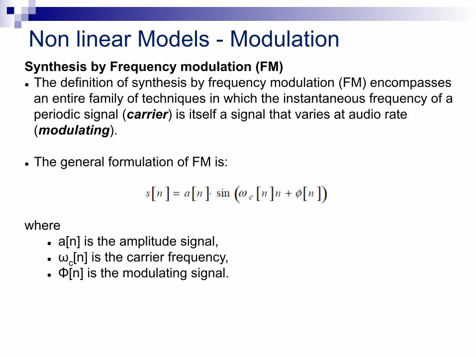
Non linear Models - Modulation Synthesis by Frequency modulation (FM) l  The definition of synthesis by frequency modulation (FM) encompasses

an entire family of techniques in which the instantaneous frequency of a periodic signal (carrier) is itself a signal that varies at audio rate (modulating).

l  The general formulation of FM is: where

l  a[n] is the amplitude signal, l  ωc[n] is the carrier frequency, l  Φ[n] is the modulating signal.

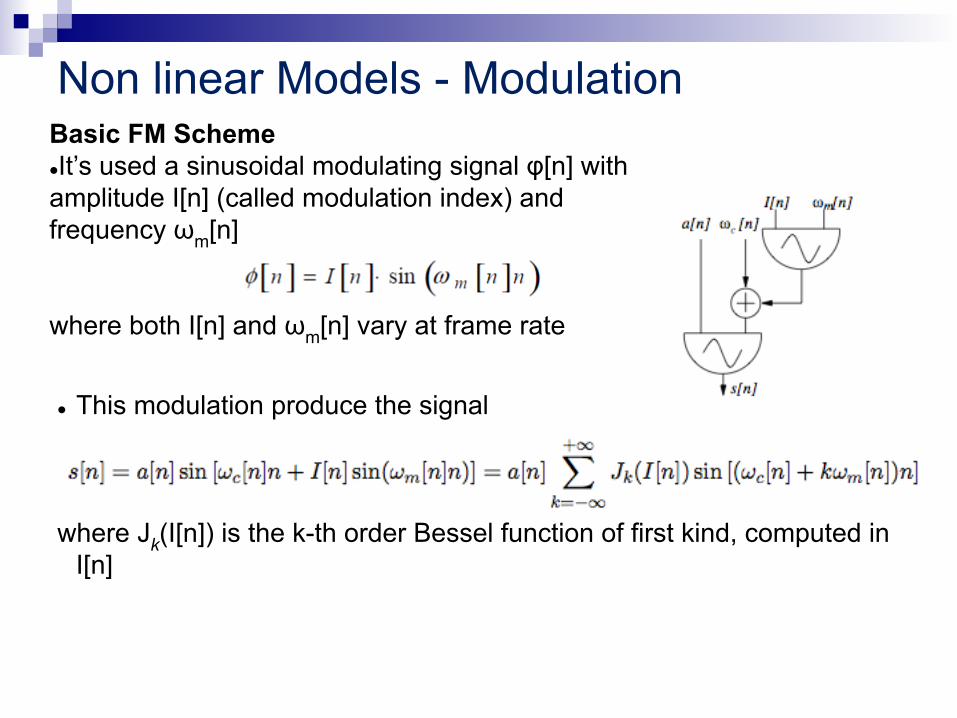
Non linear Models - Modulation Basic FM Scheme l It’s used a sinusoidal modulating signal φ[n] with amplitude I[n] (called modulation index) and frequency ωm[n] where both I[n] and ωm[n] vary at frame rate

l  This modulation produce the signal where Jk(I[n]) is the k-th order Bessel function of first kind, computed in

I[n]

Non linear Models - Modulation Basic FM Scheme l we can see that the resulting spectrum is composed of partials at frequencies | ωc ± kωm |, each with amplitude Jk(I)

l Note that an infinite number of partials is generated, so that the signal bandwidth is not limited. In practice however only a few low-order Bessel functions take significantly non-null values for small values of I

l As I increases, the number of significantly non-null Bessel functions increases too. So we can control the bandwidth around ωc

l we can control inharmonic factor through the ratio ωc / ωm

Non linear Models - Modulation Compound modulation l If the modulating signal is composed of two sinusoids l s[n] possesses the partials with frequencies |ωc ± k1ω1 ± k2ω2| with amplitudes given by

l Simplification: consider ω1>ω2 and consider only the sinusoid with ω1. We obtain partials with frequencies |ωc ± k1ω1|. Adding the second sinusoid, each partial of the first one become a carry for the second one

l If ωc is the greatest common divider for ω1 and ω2 then the spectrum is |ωc ± kωm| similar to the basic case, but with a more rich spectrum

l Otherwise we produce inharmonic components

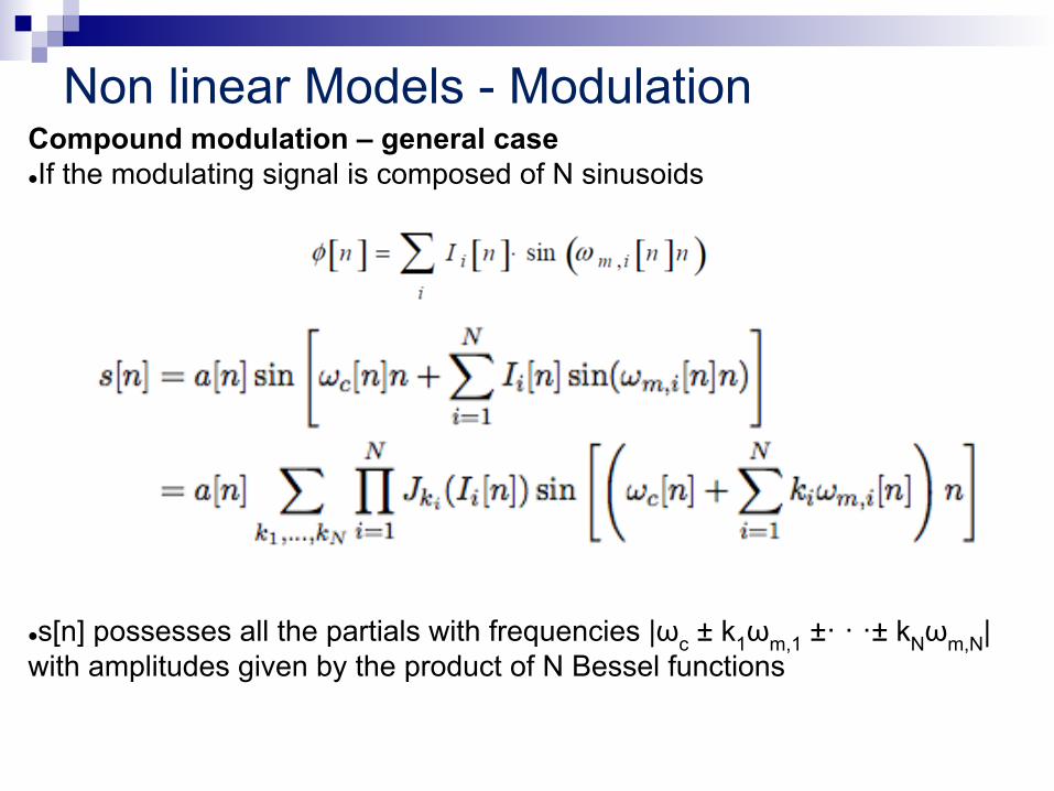
Non linear Models - Modulation Compound modulation – general case l If the modulating signal is composed of N sinusoids l s[n] possesses all the partials with frequencies |ωc ± k1ωm,1 ±· · ·± kNωm,N| with amplitudes given by the product of N Bessel functions

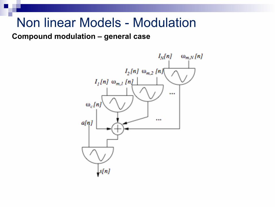
Non linear Models - Modulation Compound modulation – general case

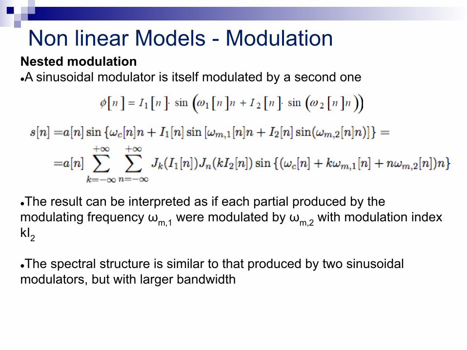
Non linear Models - Modulation Nested modulation l A sinusoidal modulator is itself modulated by a second one l The result can be interpreted as if each partial produced by the modulating frequency ωm,1 were modulated by ωm,2 with modulation index kI2

l The spectral structure is similar to that produced by two sinusoidal modulators, but with larger bandwidth

Non linear Models - Modulation Nested modulation

Non linear Models - Modulation Feedback modulation l Past values of the output signal are used as a modulating signal l With n0=1

l and β (called the feedback factor) acts as a scale factor or feedback modulation index.

l For increasing values of β the resulting signal is periodic of frequency ωc and changes smoothly from a sinusoid to a sawtooth waveform. Moreover one may vary the delay n0 in the feedback, and observe emergence of chaotic behaviors for suitable combinations of the parameters n0 and β.

Sound Modeling: signal-based approaches (part...

Documents

Transcript of Sound Modeling: signal-based approaches (part...