Some Vertex-Degree-Based Topological Indices of...
137
National University of Computer and Emerging Sciences, Lahore Campus Department of Sciences and Humanities Some Vertex-Degree-Based Topological Indices of Graphs Submitted by Akbar Ali In partial fulfillment of the requirements for the degree of Doctor of Philosophy in Mathematics (February, 2016)
Transcript of Some Vertex-Degree-Based Topological Indices of...
National University of Computer and Emerging Sciences,Lahore Campus
Department of Sciences and Humanities
Some Vertex-Degree-Based TopologicalIndices of Graphs
Submitted by
Akbar Ali
In partial fulfillment of the requirements for the degree of
Doctor of Philosophyin
Mathematics(February, 2016)


Author’s Declaration
I, Akbar Ali, declare that this dissertation was carried out in accordance with therules and regulations of the National University of Computer and Emerging Sciences.The work is original except where indicated by special references in the text and no partof the dissertation has been submitted for any other degree. The dissertation has notbeen presented to any other University for examination.
Dated: February, 2016
Author:Akbar Ali
Plagiarism Undertaking
I, Akbar Ali, solemnly declare that the research work presented in the PhDThesis titled “Some Vertex-Degree-Based Topological Indices of Graphs” has beencarried out solely by myself with no significant help from any other person exceptfew of those which are duly acknowledged. I confirm that no portion of my thesishas been plagiarized and any material used in the Thesis from other sources is properlyreferenced.
Dated: February, 2016
Author:Akbar Ali

Dedicated
To
My Parents
and
My Brother Nasir Mahmood

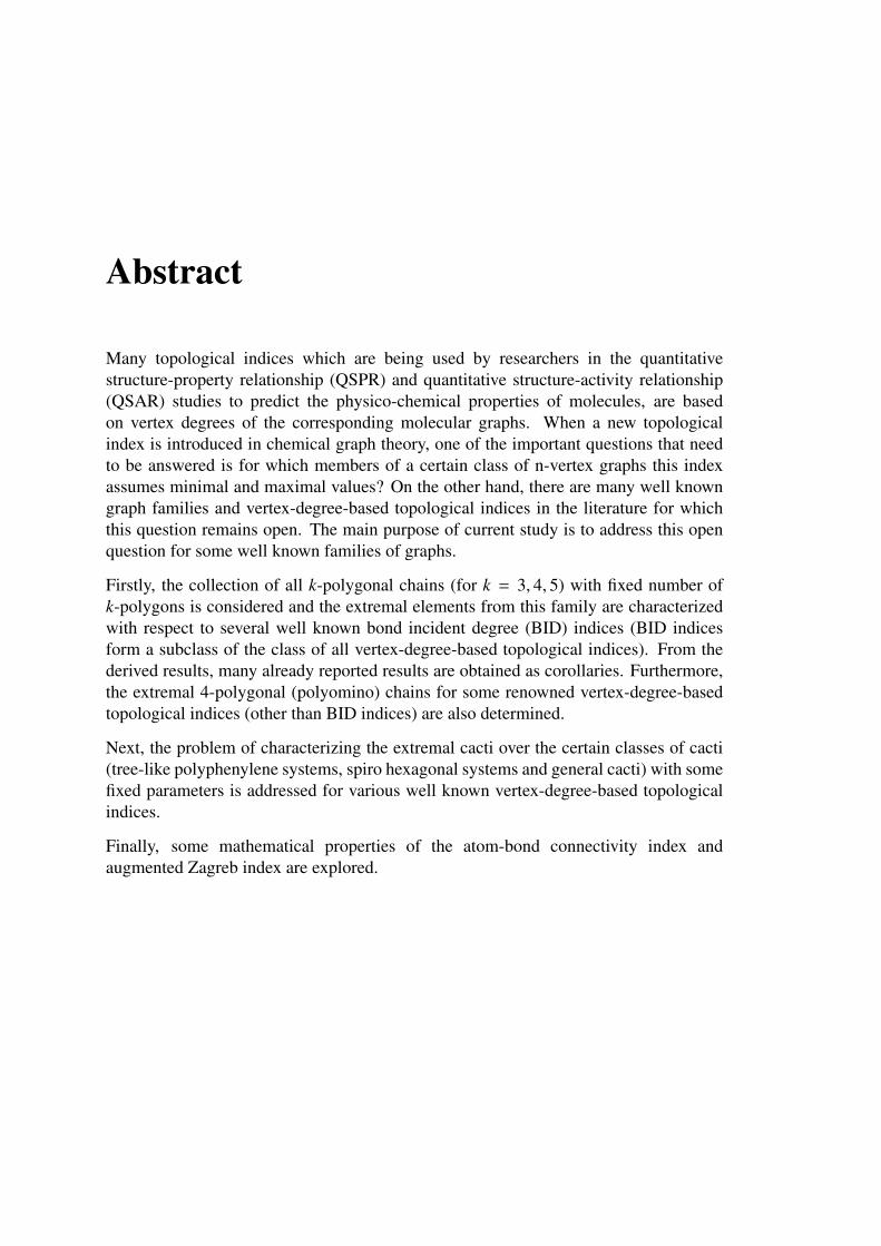
Abstract
Many topological indices which are being used by researchers in the quantitativestructure-property relationship (QSPR) and quantitative structure-activity relationship(QSAR) studies to predict the physico-chemical properties of molecules, are basedon vertex degrees of the corresponding molecular graphs. When a new topologicalindex is introduced in chemical graph theory, one of the important questions that needto be answered is for which members of a certain class of n-vertex graphs this indexassumes minimal and maximal values? On the other hand, there are many well knowngraph families and vertex-degree-based topological indices in the literature for whichthis question remains open. The main purpose of current study is to address this openquestion for some well known families of graphs.
Firstly, the collection of all k-polygonal chains (for k = 3, 4, 5) with fixed number ofk-polygons is considered and the extremal elements from this family are characterizedwith respect to several well known bond incident degree (BID) indices (BID indicesform a subclass of the class of all vertex-degree-based topological indices). From thederived results, many already reported results are obtained as corollaries. Furthermore,the extremal 4-polygonal (polyomino) chains for some renowned vertex-degree-basedtopological indices (other than BID indices) are also determined.
Next, the problem of characterizing the extremal cacti over the certain classes of cacti(tree-like polyphenylene systems, spiro hexagonal systems and general cacti) with somefixed parameters is addressed for various well known vertex-degree-based topologicalindices.
Finally, some mathematical properties of the atom-bond connectivity index andaugmented Zagreb index are explored.


Acknowledgements
I wish to place my deep sense of admiration to my advisor Dr. Akhlaq Ahmad Bhatti,for his constant support and ample guidance during this research. He showed a lot ofconfidence in me and always supported me.
Akbar AliM.Phil (Math)


Table of Contents
Table of Contents xi
List of Figures xiii
List of Tables xv
Abbreviations and Nomenclature xvii
1 Introduction 11.1 Motivation and Problems Statement . . . . . . . . . . . . . . . . . . . 21.2 Organization of the Thesis . . . . . . . . . . . . . . . . . . . . . . . . 3
2 Some Elements of Graph Theory 52.1 Basic Notions . . . . . . . . . . . . . . . . . . . . . . . . . . . . . . . 52.2 Subgraphs . . . . . . . . . . . . . . . . . . . . . . . . . . . . . . . . . 62.3 Isomorphic Graphs . . . . . . . . . . . . . . . . . . . . . . . . . . . . 72.4 Some Graph Operations . . . . . . . . . . . . . . . . . . . . . . . . . . 72.5 Some Common Families of Graphs . . . . . . . . . . . . . . . . . . . . 72.6 Connected and Disconnected Graphs . . . . . . . . . . . . . . . . . . . 82.7 Trees . . . . . . . . . . . . . . . . . . . . . . . . . . . . . . . . . . . . 82.8 Cyclomatic Number . . . . . . . . . . . . . . . . . . . . . . . . . . . . 82.9 Line Graphs . . . . . . . . . . . . . . . . . . . . . . . . . . . . . . . . 82.10 Vertex Connectivity and Matching Number . . . . . . . . . . . . . . . 9
3 Literature Review 113.1 Vertex-Degree-Based Topological Indices . . . . . . . . . . . . . . . . 113.2 k-Polygonal Chains . . . . . . . . . . . . . . . . . . . . . . . . . . . . 133.3 Cacti . . . . . . . . . . . . . . . . . . . . . . . . . . . . . . . . . . . . 143.4 The ABC index and AZI . . . . . . . . . . . . . . . . . . . . . . . . . 14
xi
4 Some Vertex-Degree-Based Topological Indices of k-Polygonal Chains 174.1 Triangular Chains . . . . . . . . . . . . . . . . . . . . . . . . . . . . . 184.2 Polyomino Chains . . . . . . . . . . . . . . . . . . . . . . . . . . . . . 294.3 Pentagonal Chains . . . . . . . . . . . . . . . . . . . . . . . . . . . . 44
5 Some Vertex-Degree-Based Topological Indices of Cacti 535.1 Two Special Cacti: Tree-Like Polyphenylene and Spiro Hexagonal
Systems . . . . . . . . . . . . . . . . . . . . . . . . . . . . . . . . . . 535.2 General Formulae for Calculating BID Indices of Polyphenylene
Dendrimer Nanostars . . . . . . . . . . . . . . . . . . . . . . . . . . . 585.3 Extremal General Cacti for Some Vertex-Degree-Based Topological
Indices . . . . . . . . . . . . . . . . . . . . . . . . . . . . . . . . . . . 61
6 On the ABC index and AZI 736.1 The ABC Index . . . . . . . . . . . . . . . . . . . . . . . . . . . . . . 736.2 The AZI of Chemical Bicyclic and Unicyclic graphs . . . . . . . . . . . 806.3 Nordhaus-Gaddum Type Results for AZI . . . . . . . . . . . . . . . . . 886.4 The AZI and Vertex Connectivity . . . . . . . . . . . . . . . . . . . . . 906.5 The AZI and Matching Number . . . . . . . . . . . . . . . . . . . . . 946.6 The AZI of Cacti . . . . . . . . . . . . . . . . . . . . . . . . . . . . . 966.7 Sharp Bounds for the AZI in Terms of Some Other Well-Known BID
Indices . . . . . . . . . . . . . . . . . . . . . . . . . . . . . . . . . . . 99
7 Conclusions and Future Research Directions 1037.1 Summary of the Novel Contributions . . . . . . . . . . . . . . . . . . . 1037.2 Future Research Directions . . . . . . . . . . . . . . . . . . . . . . . . 104
Bibliography 106

List of Figures
4.1 A pentagonal system. . . . . . . . . . . . . . . . . . . . . . . . . . . . 174.2 All the segments of a triangular chain. . . . . . . . . . . . . . . . . . . 184.3 The edges in the first segment, which may be of the type (3,5) are
labeled as e1, e2, e3, e4. . . . . . . . . . . . . . . . . . . . . . . . . . . 204.4 The edges in the ith segment (where 2 ≤ i ≤ s − 2 and s ≥ 4), which
may be of the type (3,5) are labeled as e5, e6, e7. . . . . . . . . . . . . . 204.5 A linear polyomino chain . . . . . . . . . . . . . . . . . . . . . . . . . 294.6 A zigzag polyomino chain . . . . . . . . . . . . . . . . . . . . . . . . 294.7 Partition of the edges of a polyomino chain . . . . . . . . . . . . . . . 314.8 Partitioning the edge set of a pentagonal chain P5,19 . . . . . . . . . . . 464.9 The graph transformation T1. . . . . . . . . . . . . . . . . . . . . . . . 49
5.1 (a) A tree-like polyphenylene system T PS 7. (b) Spiro hexagonal systemS S 7 corresponding to T PS 7 given in (a). . . . . . . . . . . . . . . . . . 54
5.2 The graph transformations Ti where i = 1, 2, ..., 8. In all the graphs,edges incident with C will be coincident if C does not contain any hexagon. 56
5.3 The tree-like polyphenylene system T PS ∗h′ where h′ = 2 + 5t1 and t1 ≥ 1. 575.4 The molecular graph NS 1[2] of the first type of polyphenylene
dendrimer nanostar with two generations. . . . . . . . . . . . . . . . . 595.5 The molecular graph NS 2[2] of the second type of polyphenylene
dendrimer nanostar with two steps of growth. . . . . . . . . . . . . . . 605.6 The cactus G0(n, k). . . . . . . . . . . . . . . . . . . . . . . . . . . . . 61
6.1 The molecular graphs K1,4 and T ∗ . . . . . . . . . . . . . . . . . . . . 736.2 Two graphs B1
n and B2n, used in the proof of Lemma 6.2.1 . . . . . . . . 81
6.3 Chemical bicyclic graph B′n where n = 5k + 26. . . . . . . . . . . . . . 82
6.4 Chemical unicyclic graph U′n where n = 5k + 15. . . . . . . . . . . . . 87
xiii
xiv

List of Tables
6.1 The values of θi j and ϕi j for all edges with degrees (di, d j) where 5 ≤di ≤ 6 and di ≥ d j . . . . . . . . . . . . . . . . . . . . . . . . . . . . . 75
6.2 The values of θi j and ϕi j for all edges with degrees (di, d j) where 2 ≤di ≤ 4 and di ≥ d j . . . . . . . . . . . . . . . . . . . . . . . . . . . . . 75
xv

xvi

Abbreviations and Nomenclature
List of Abbreviations
Abbreviation Description
QSPR Quantitative Structure-Property Relationship
QSAR Quantitative Structure-Activity Relationship
BID Bond Incident Degree
ABC Atom-Bond Connectivity
AZI Augmented Zagreb Index
RRR (Index) Reduced Reciprocal Randic (Index)
List of Symbols
Symbol Description
Pk,n A k-polygonal chain with n k-polygons
Tn Collection of all those 3-polygonal chains with n ≥ 4triangles in which every vertex has degree at most five
S i The ith segment of a k-polygonal chain
l(S i) or li Length of the ith segment S i of a k-polygonal chain
xvii

Symbol Description
Lk,n Linear k-polygonal chain
Zk,n Zigzag k-polygonal chain
Ωn Collection of all those 4-polygonal chains (with n ≥ 3squares) in which no internal segment of length threehas edge connecting the vertices of degree three
T PS h Tree-like polyphenylene system with h ≥ 2 hexagons
S S h Spiro hexagonal system corresponding to T PS h
PCh Polyphenylene chain with h ≥ 2 hexagons
S Ch Spiro hexagonal chain with h ≥ 2 hexagons
Cn,k Collection of all cacti with k cycles and n ≥ 5 vertices
C∗n,k Sub-collection of Cn,k, containing those cacti in whichall the pendant vertices are adjacent with the same vertex
G0(n, k) Cactus obtained from the star S n by adding k mutuallyindependent edges
κ Vertex connectivity
Γn,κ Class of all graphs with n ≥ 3 vertices and κ ≥ 2
β Matching number
Υn,β Family of all connected graphs with n ≥ 4 vertices andmatching number β, where 2 ≤ β ≤ ⌊ n
2⌋
T I Bond Incident Degree Index
M1 First Zagreb Index
M2 Second Zagreb Index
xviii

Symbol Description
R Randic Index
H Harmonic Index
A Albertson Index
ABC Atom-Bond Connectivity Index
M∗2 Modified Second Zagreb Index
χ Sum-Connectivity Index
GA First Geometric-Arithmetic Index
AZI Augmented Zagreb Index
Π1 First Multiplicative Zagreb Index
Π∗1 Modified First Multiplicative Zagreb Index
Π2 Second Multiplicative Zagreb Index
RRR Reduced Reciprocal Randic Index
irrt Total irregularity
NK Narumi-Katayama index
0Rα Zeroth-order general Randic index
xix

xx

Chapter 1
Introduction
Graph theory is a branch of mathematics. Our journey into this theory starts with apuzzle (known as the seven bridges of Konigsberg puzzle) that was solved by LeonhardEuler in 1735 and with his solution he laid the foundation of what is now known asgraph theory. Later, the concept of graph was independently introduced by GustavRobert Kirchhoff while he was working on electrical circuits and Arthur Cayley who atthat time was working on enumeration of organic isomers.
Graph theory is widely employed in the study of networks, patterns, electric circuits,scheduling and routings as diverse as linen supply and garbage collection. This theoryhas found considerable applications in computer science, chemistry, physics, electricaland civil engineering, communication science, operational research, architecture,genetics, sociology, psychology, anthropology, linguistics and economics. In the presentstudy, we are concerned with the part of graph theory that can be applied in chemistrywhich is called chemical graph theory.
In 1874, Alexander Crum Brown (one of the great pioneers of chemical structurestheory) prognosticated “... chemistry will become a branch of applied mathematics;but it will not cease to be an experimental science. Mathematics may enable usretrospectively to justify results obtained by experiment, may point out useful lines ofresearch and even sometimes predict entirely novel discoveries. We do not know whenthe change will take place, or whether it will be gradual or sudden...”. This prophecywas soon to be fulfilled when, in the same year, Arthur Cayley published the article“On the Mathematical Theory of Isomers”, which represents the first serious chemicalapplication of graph theory. Arthur Cayley was interested in the number of possiblealkane structures for a given number of carbon atoms and for this purpose he introducedgraph-theoretical notions to represent alkane structures. In parallel, he gave an idea torepresent molecular structures using graphs. Thus, he simplified the chemical problemto a graph-theoretical one.
1

1. Introduction
In theoretical chemistry, molecular descriptors are often used to develop quantitativestructure-property relationship (QSPR) and quantitative structure-activity relationship(QSAR). These descriptors are also used to establish the mathematical basis forconnections between molecular structures and physico-chemical properties. Accordingto Todeschini and Consonni (2000) “The molecular descriptor is the final result of alogical and mathematical procedure which transforms chemical information encodedwithin a symbolic representation of a molecule into an useful number or the result ofsome standardized experiment”. A graph-based molecular descriptor is simply knownas a topological index (Estrada and Bonchev 2013). In graph theoretical notation,topological indices are the numerical parameters of a graph which are invariant undergraph isomorphisms. “Topological indices are expected to correlate with physicalobservable measures by experiments in a way that theoretical predictions can be usedto gain chemical insights even for not yet existing molecules” (Estrada and Bonchev2013).
A vast number of topological indices exists in the literature (Todeschini and Consonni2000; Consonni 2009; Gutman and Furtula 2010). But, in this thesis, we pay ourattention to only vertex-degree-based topological indices. These are the topologicalindices which depend on only vertex degrees of the graph.
1.1 Motivation and Problems StatementWhen a new topological index is introduced in mathematical chemistry, one of theimportant questions that needs to be answered is for which members of a certain classof n-vertex graphs this index assumes minimal and maximal values? On the other hand,there are many well known graph families and vertex-degree-based topological indicesin the literature for which this question remains open. The main motivation for thecurrent study comes from this fundamental question.
In this dissertation, the following major problems are addressed:
Problem 1.1.1. Characterization of the graphs having the maximum and minimumcertain vertex-degree-based topological index among the class of all
• k-polygonal chains (for k = 3, 4, 5) with fixed number of k-polygons,
• n-vertex cacti having fixed number of cycles,
• n-vertex chemical unicyclic and bicyclic graphs,
• tree-like polyphenylene systems and spiro hexagonal systems with fixed numberof hexagons.
2
1.2 Organization of the Thesis
Problem 1.1.2. Finding sharp bounds on the atom-bond connectivity index andaugmented Zagreb index in terms of some other graph parameters.
1.2 Organization of the ThesisThe thesis is organized in seven chapters. In Chapter 1, background, motivation andproblem statements are presented. Some necessary definitions and auxiliary results fromgraph theory are given in the Chapter 2. Chapter 3 is devoted to a brief literature reviewof the related work.
Chapter 4 is dedicated to characterize the extremal k-polygonal chains (for k = 3, 4, 5)with respect to several well known bond incident degree (BID) indices (BID indicesform a subclass of vertex-degree-based topological indices). Furthermore, the extremal4-polygonal (polyomino) chains for some renowned vertex-degree-based topologicalindices (other than BID indices) are also determined in this chapter. Some results fromthis chapter are published in papers (Ali et al. 2014c, 2015b) and other results of thischapter are submitted for publication (Ali et al. 2014a; Ali and Bhatti 2015; Ali et al.2015a).
The problem of characterizing the extremal cacti for various well known vertex-degree-based topological indices over the certain collections of cacti with some fixedparameters is addressed in the Chapter 5. From this chapter, some results are published(Ali et al. 2014c), some are accepted for publication (Ali et al. 2016c) and the remainingones are submitted for publication (Ali et al. 2014d).
In Chapter 6, some mathematical properties of the atom-bond connectivity index andaugmented Zagreb index are explored. Some work from this chapter has been acceptedfor publication (Ali et al. 2016a,b; Raza et al. 2016; Ali and Bhatti 2016) and theremaining work from this chapter is submitted for publication (Ali et al. 2014b).
In Chapter 7, some research directions are proposed with reference to the currentresearch work.
3

1. Introduction
4

Chapter 2Some Elements of Graph Theory
2.1 Basic NotionsThere are many definitions of a graph available in the literature but we mention here onegiven in (Agnarsson and Greenlaw 2006).
Definition 2.1.1. A graph or general graph is an ordered triple G = (V, E, ϕ), where
1. V and E are disjoint sets provided that V is non-empty,
2. ϕ is function from E to P(V) (power set of V) such that for every e ∈ E, ϕ(e) iseither one-element subset of V or two-element subset of V.
The elements of V are the vertices of G and the elements of E are the edges of G. Thefunction ϕ is called incidence function and the vertices in ϕ(e) are called end-verticesof the edge e. Note that two or more edges can be mapped on a single element ofP(V) under the function ϕ. Such types of edges are called multi edges or parallel edges.Moreover, if ϕ(e) is an one-element subset of V , then the edge e is called a loop. A graphwhich contains neither loop(s) nor multi edges is called simple graph. Since there is atmost one edge between a pair of vertices in a simple graph, the edges are in one-to-onecorrespondence with their different end-vertices. Hence, a simple graph can be definedwithout incidence function ϕ from the Definition 2.1.1, as follows:
Definition 2.1.2. A simple graph is an ordered pair G = (V, E), where V is a non-emptyset and E is a set of two-element subsets of V.
A graph is said to be finite if both the vertex set and edge set are finite, otherwise thegraph is called infinite. If the second condition of the Definition 2.1.1 is replaced by “ fis a function from E to V × V”, then the graph G is referred as directed graph.
Note 2.1.3. In the rest of thesis, by the term “graph” we will always mean a simple,finite and undirected graph.
5

2. Some Elements of Graph Theory
The vertex set and edge set of a graph G are denoted by V(G) and E(G) respectively. Ife = u, v is an edge of G, then u and v are adjacent vertices and the edge e is incidentwith each of the two vertices u and v. Two edges are adjacent if they share a vertex. Itis convenient to denote an edge by e = uv or e = vu rather than e = u, v. The numberof elements in V(G) (respectively E(G)) is called the order (respectively size) of G andis commonly denoted by n(G) (respectively m(G)) or simply by n (respectively m). Agraph having order n is called n-vertex graph. Since the vertex set of a graph is non-empty, the order of every graph is at least 1. A graph with exactly one vertex is called atrivial graph.
The degree of a vertex vi ∈ V(G) is the number of vertices adjacent with vi and isdenoted by dvi or simply by di. A vertex of degree 0 is referred to as an isolated vertexand a vertex with degree 1 is called pendent vertex. An edge is said to be pendant ifone of its vertices is pendant. For a vertex u of a graph G, the neighborhood of u isdenoted by NG(u) and is defined as the set of all vertices adjacent with u. The maximumand minimum vertex degree in a graph G is denoted by ∆(G) and δ(G) (or simply by ∆and δ) respectively. A graph in which the maximum vertex degree is at most 4 is calledchemical or molecular graph. If the graph G has order n and v is any vertex of G, then
0 ≤ δ ≤ dv ≤ ∆ ≤ n − 1.
Since every edge in a graph is incident with exactly two vertices, when the degrees ofall vertices are summed then each edge is counted twice. Hence, we have:
Theorem 2.1.4. If a graph G has m edges, then∑v∈V(G)
dv = 2m.
The number of vertices of degree i in a graph G is denoted by ni(G) or simply by ni andthe number of edges connecting the vertices of degrees i and j is denoted by xi, j(G) orsimply by xi, j.
2.2 SubgraphsA graph H is said to be a subgraph of a graph G if V(H) ⊆ V(G) and E(H) ⊆ E(G). Ifa subgraph H of G has the same order as G, then H is called a spanning subgraph of G.A subgraph H of a graph G is called an induced subgraph of G if whenever u, v ∈ V(H)and uv ∈ E(G), then uv ∈ E(H). If v ∈ V(G) and G has at least two vertices, thenG − v denotes the graph obtained from G by removing the vertex v (and of-course its
6

2.3 Isomorphic Graphs
incident edges). If u, v ∈ V(G) such that uv ∈ E(G) (respectively uv < E(G)) then G−uv(respectively G+uv) is the graph obtained from G by removing (respectively by adding)the edge uv. If A ⊂ V(G) and B ⊆ E(G), then the graphs G−A and G−B can be definedanalogously. It is easy to see that G − A is an induced subgraph and G − B is a spanningsubgraph of G. Furthermore, G can be considered as a spanning subgraph of G + uv.
2.3 Isomorphic Graphs
A graph G1 is said to be isomorphic to a graph G2 (symbolically written as G1 G2) ifthere exists a bijective mapping ψ : V(G1)→ V(G2) such that uv ∈ E(G1) if and only ifψ(u)ψ(v) ∈ E(G2).
2.4 Some Graph Operations
The union H ∪ K of two graphs H and K is the graph with the vertex set V(H) ∪ V(K)and the edge set E(H)∪ E(K). The join H + K of two graphs H and K is the graph withthe vertex set V(H) ∪ V(K) and the edge set E(H) ∪ E(K) ∪ uv|u ∈ V(H), v ∈ V(K).The complement G of a graph G has the vertex set V(G) = V(G) and the edge setE(G) = uv|uv < E(G).
2.5 Some Common Families of Graphs
A graph G is r-regular (or simply regular) if du = r for every vertex u of G. A graphG is complete if every two vertices of G are adjacent. A complete graph of order n isdenoted by Kn.
Let u and v be vertices of a graph G. A subgraph of G is said to be a u− v path P in G ifV(P) = u = u0, u1, u2, ..., uk−1, uk = v (where ui , u j for i , j) and E(P) = ui−1ui|1 ≤i ≤ k. The size of a path is also called its length. A path of order n is usually denotedby Pn. By adding one edge uv in a u − v path yields the concept of a cycle. A cycle oforder n is denoted by Cn. A cycle of order three is also called triangle. A graph havingno cycle is known as acyclic graph.
A graph G is bipartite if the vertex set of G can be partitioned into two sets V1 and V2 insuch a way that no two vertices from the same set are adjacent. Such partition (V1,V2)is known as bipartition of G. A complete bipartite graph Kp,q is a bipartite graph withbipartition (V1,V2) where |V1| = p and |V2| = q such that each vertex of V1 is adjacent toevery vertex of V2. Note that Kp,q Kq,p.
7

2. Some Elements of Graph Theory
2.6 Connected and Disconnected GraphsTwo vertices u and v of a graph G are said to be connected if there exists a u − v pathin G. The graph G is connected if every two vertices of G are connected. A graphthat is not connected is called disconnected. A component of a graph G is a connectedsubgraph of G not contained in any other connected subgraph of G.
A vertex v of a graph G is a cut-vertex if G − v contains more components than G.Analogously, an edge e of a graph G is a bridge if G− e contains more components thanG.
2.7 TreesAn acyclic and connected graph is called tree. The path Pn and complete bipartite graphK1,q (which is usually denoted by S q+1 and is also called star) are trees. A tree in whichexactly one of its vertices has degree greater than two is known as Starlike tree. LetS (r1, r2, . . . , rk) denote the Starlike tree which has a vertex v of degree k > 2 such thatthe graph obtained from S (r1, r2, . . . , rk) by removing the vertex v is Pr1 ∪ Pr2 ∪ · · · ∪ Prk
where Pri is the path graph on ri (1 ≤ i ≤ k) vertices. We say that the Starlike treeS (r1, r2, . . . , rk) has k branches, the lengths of which are r1, r2, . . . , rk (r1 ≥ r2 ≥ · · · ≥rk ≥ 1) and has
∑ki=1 ri + 1 vertices.
2.8 Cyclomatic NumberFor a graph G, the cyclomatic number (also known as first Betti number and circuitrank) is denoted by µ(G) and is defined as the minimum number of edges which mustbe removed from G so that G becomes acyclic graph. Hence, if G has n vertices, medges and k components then
µ(G) = m − n + k.
From the definition of µ(G), it is clear that if G is a tree then µ(G) = 0. If µ(G) = 1(respectively µ(G) = 2) then G is called unicyclic (respectively bicyclic). Furthermore,if G is connected unicyclic (respectively bicyclic) graph then m = n (respectively m =n + 1).
2.9 Line GraphsThe line graph L(G) of a graph G has the vertex set V(L(G)) = E(G) where the twovertices of L(G) are adjacent if and only if the corresponding edges of G are adjacent. Atriangle of a graph G is called odd if there is a vertex of G adjacent to an odd number of
8

2.10 Vertex Connectivity and Matching Number
its vertices. The following theorem gives one of the important characterizations of linegraphs.
Lemma 2.9.1. (Harary 1969) A graph G is a line graph if and only if G does not haveK1,3 as an induced subgraph and if two odd triangles have a common edge then thesubgraph induced by their vertices is K4.
Detailed properties of line graphs can be found in (Harary 1969). Some possiblechemical applications of line graphs of molecular graphs are given in (Gutman andEstrada 1996).
2.10 Vertex Connectivity and Matching NumberThe vertex connectivity (commonly referred to as connectivity) of a graph G is denotedby κ(G) (or simply by κ) and is defined as the minimum number of vertices whoseremoval gives rise to a disconnected or trivial graph. If G is disconnected then κ(G) = 0.
A matching in a graph is a set of pairwise non-adjacent edges. A maximum matchingis one which covers as many vertices as possible. The matching number of a graphG is denoted by β(G) (or simply by β) and is defined as the number of edges in amaximum matching. A component of a graph is odd (respectively even) if it has an odd(respectively even) number of vertices. If n is the order of the graph G and o(G) is thenumber of odd components, then by Tutte-Berge formula (Lovasz and Plummer 1986),
n − 2β(G) = maxo(G − A) − |A| : A ⊂ V(G). (2.10.1)
9

2. Some Elements of Graph Theory
10

Chapter 3Literature Review
In this chapter, detailed review of literature on the vertex-degree-based topologicalindices for various types of graph families is presented.
3.1 Vertex-Degree-Based Topological IndicesUsage of topological indices in chemistry began in 1947 when the chemist Wiener(1947) introduced the most widely known topological index, the Wiener index, forcalculating the boiling points of types of alkanes known as paraffins. After the successof Wiener index, numerous topological indices have been proposed (Gutman 2013;Todeschini and Consonni 2000; Consonni 2009; Gutman and Furtula 2010). Manytopological indices which are being used by researchers in the quantitative structure-property relationship (QSPR) and quantitative structure-activity relationship (QSAR)studies to predict the physico-chemical properties of molecules, are based on vertexdegrees of the corresponding molecular graphs (Gutman 2013; Gutman and Furtula2010), which are called vertex-degree-based topological indices. A considerableamount of these vertex-degree-based topological indices can be represented as the sumof edge contributions of graph (Hollas 2005; Vukicevic and Gasperov 2010). These kindof vertex-degree-based topological indices are known as bond incident degree indices(BID indices in short) (Vukicevic and Gasperov 2010; Vukicevic 2010; Vukicevic andDurdevic 2011) whose general form (Hollas 2005) is:
T I = T I(G) =∑
uv∈E(G)
f (du, dv) =∑
1≤a≤b≤∆(G)
xa,b(G).θa,b , (3.1.1)
where θa,b is a non-negative real valued function depending on a, b. Many well knowntopological indices can be obtained from (3.1.1) by taking suitable function θa,b. Forinstance, we mention here some special cases of (3.1.1) in which the function θa,b isdefined in the following manner (γ is a non zero real number):
11

3. Literature Review
θa,b = a + b First Zagreb index (Gutman and Trinajstic 1972)
θa,b = ab Second Zagreb index (Gutman et al. 1975)
θa,b =1√ab
Randic index (Randic 1975)
θa,b =2
a+b Harmonic index (Fajtlowicz 1987)
θa,b =| a − b | Albertson index (Albertson 1997)
θa,b = (ab)γ General Randic index (Bollobas and Erdos 1998)
θa,b =
√a+b−2
ab Atom-bond connectivity index (Estrada et al. 1998)
θa,b =1ab Modified second Zagreb index (Nikolic et al. 2003)
θa,b =1√a+b
Sum-connectivity index (Zhou and Trinajstic 2009)
θa,b =√
ab12 (a+b)
First geometric-arithmetic index (Vukicevic and Furtula 2009)
θa,b = (a + b)γ General sum-connectivity index (Zhou and Trinajstic 2010)
θa,b =(
aba+b−2
)3Augmented Zagreb index (Furtula et al. 2010)
θa,b = ln(ab) Logarithm of second multiplicative Zagreb index (Gutman 2011)
θa,b =(
a+b−2ab
)γGeneral atom-bond connectivity index (Xing and Zhou 2012)
θa,b = ln (a + b) Logarithm of modified first multiplicative Zagreb index (Eliasi et al. 2012)
θa,b =√
(a − 1)(b − 1) Reduced Reciprocal Randic index (Manso et al. 2012; Gutman et al. 2014)
Here, it should be noted that the modified second Zagreb index is equal to the first-order overall index (Bonchev 2001; Nikolic et al. 2003). In addition to above listed BIDindices, a whole class of BID indices is recently proposed (Vukicevic and Gasperov2010) and several indices from this class were examined for chemical applicability.Besides, many indices of the form (3.1.1) exist in the literature. Details about the BIDindices can be found in the recent review (Gutman 2013), articles (Deng et al. 2011;Rada et al. 2013; Furtula et al. 2013; Gutman and Tosovic 2013; Gutman et al. 2014;Zhong and Xu 2014) and the references cited therein. In addition to the BID indices,several well known vertex-degree-based topological indices are defined in either of thefollowing forms:
T I = T I(G) =∑
u,v∈V(G)
f (du, dv), (3.1.2)
T I = T I(G) =∑
u∈V(G)
f (du). (3.1.3)
For example, the choice f (du, dv) = |du−dv |2 in Eq.(3.1.2) gives total irregularity (Abdo
et al. 2014) and the choices f (du) = ln(du), f (du) = 2ln(du), f (du) = (du)α in Eq.(3.1.3)give logarithm of Narumi-Katayama index (Narumi and Katayama 1984), logarithm
12

3.2 k-Polygonal Chains
of first multiplicative Zagreb index (Gutman 2011), zeroth-order general Randic index(Li and Zheng 2005) respectively, where α is any real number different from 0 and1. At this point it is worth mentioning that the inverse degree (Fajtlowicz 1987) (alsoknown as modified total adjacency index (Nikolic et al. 2003)), modified first Zagrebindex (Nikolic et al. 2003), first Zagreb index (Gutman and Trinajstic 1972), forgottentopological index (Furtula and Gutman 2015) and variable first Zagreb index (Milicevicand Nikolic 2004) can be obtained from the zeroth-order general Randic index by takingcertain values of α. Furthermore, it is notable that the first multiplicative Zagreb indexis equal to the square of the Narumi-Katayama index. On the other hand, according toDoslic et al. (2011): ∑
u∈V(G)
f (du) =∑
uv∈E(G)
(f (du)du+
f (dv)dv
).
It means that all the indices of the form (3.1.3) are also BID indices. Is every vertex-degree-based topological index a BID index or of the form (3.1.2)? The answer isnegative; the higher order Randic indices (Kier et al. 1976) and Zagreb coindices(Doslic 2008) are neither BID indices nor can be obtained from the Eq.(3.1.2), butthey are vertex-degree-based topological indices. However, in this thesis, we restrictour attention to only total irregularity, Narumi-Katayama index, multiplicative Zagrebindices and BID indices.
3.2 k-Polygonal Chains
The problems of finding closed form formulae for calculating the different vertex-degree-based topological indices of k-polygonal chains (especially 4-polygonal chains,which are also known as polyomino chains) and characterizing the extremal chainswith respect to the aforementioned indices over the set of all k-polygonal chains withfixed number of k-polygons have attracted substantial attention from researchers inrecent years. For instance, Yarahmadi et al. (2012) established efficient formulae forcalculating the first and second Zagreb indices of polyomino chains and characterizedthe extremal polyomino chains with respect to the first and second Zagreb indices. Theextremal 6-polygonal chains (also known as hexagonal chains and benzenoid chains)with respect to vertex-degree-based topological indices were characterized in (Rada2014). Deng et al. (2014) and An and Xiong (2016) extended the work of Yarahmadiet al. (2012) for the harmonic index and general Randic index, respectively. Recently,Rada (2014) proved that the linear polyomino chain has the extremal value for manywell known BID indices.
13

3. Literature Review
3.3 CactiOver the last decade, several extremal results regarding cacti under specific constraintshave been presented for some well known vertex-degree-based topological indices.For instance, the n-vertex cactus with the minimum Randic index (respectively sum-connectivity index and atom-bond connectivity (ABC) index) among all the n-vertexcacti having fixed number of cycles were characterized in (Lu et al. 2006) (respectively(Ma and Deng 2011) and (Dong and Wu 2014)). Lin et al. (2008) discovered the n-vertex cactus having the minimum Randic index over the set of all n-vertex cacti withfixed number of pendent vertices. Li et al. (2012) determined the extremal n-vertexcacti with respect to the first and second Zagreb indices among all the n-vertex cactiwith fixed number of pendent vertices. In the same paper, the authors also identified thecactus with a perfect matching having the maximum first and second Zagreb indices.
3.4 The ABC index and AZIRecently Gutman and Tosovic (2013) tested the correlation abilities of twenty vertex-degree-based topological indices for the case of standard heats of formation and normalboiling points of octane isomers and they found that the AZI (respectively ABC index)yields the best (respectively second-best) results. Hence it is interesting to study themathematical properties of AZI and ABC index, especially bounds and characterizationof the extremal elements for different graph classes.
In (Furtula et al. 2010), the extremal properties of the AZI of trees and chemical treeswere studied. Huang et al. (2012) gave various bounds on the AZI for several familiesof connected graphs. Wang et al. (2012) established some new bounds on the AZIof connected graphs and improved some results of (Furtula et al. 2010; Huang et al.2012). Huang and Liu (2015) ordered the graphs with respect to the AZI in severalfamilies of graphs (trees, unicyclic, bicyclic and connected graphs). Zhan et al. (2015)characterized the n-vertex unicyclic with the first and second minimal AZI value andn-vertex bicyclic graphs with the minimal AZI value.
The ABC index was introduced as a modified version of the Randic index in 1998.This index did not attract any attention of researchers for almost ten years from itsdiscovery. But after the celebrated paper (Estrada 2008) a flood of publications relatedto mathematical properties of the ABC index started and are still appearing. Firstmathematical work on the ABC index was done by Furtula et al. (2009). They showedthat the n-vertex star has the maximal ABC index among all n-vertex trees and proposedan open problem related to the minimum ABC index of trees, which turned out to bevery difficult and is still open. A large number of publications were devoted to thisopen problem, see for example the recent ones (Dimitrov 2014, 2015; Magnant et al.
14

3.4 The ABC index and AZI
2015; Lin et al. 2015) and references cited therein. The problem of finding the n-vertexgraph having the maximum ABC index among all n-vertex graphs was solved by Chenand Guo (2011). The problem of characterizing the extremal elements with respectto the ABC index among different graph collections with some fixed parameters hasalso attracted a considerable attention from scholars, see for example the papers (Chenet al. 2013; Chen and Guo 2012; Ke 2012; Dehghan-Zadeh and Ashrafi 2014). Otherdirection of investigation on the ABC index include finding sharp bounds of this index interms of other graph parameters (Chen et al. 2012; Das 2010; Das et al. 2012; Palacios2014). Further details about this index can be found in the survey (Gutman et al. 2013)and references cited therein.
15

3. Literature Review
16

Chapter 4Some Vertex-Degree-Based TopologicalIndices of k-Polygonal Chains
A k-polygonal system is a connected geometric figure obtained by concatenatingcongruent regular k-polygons side to side in a plane in such a way that the figuredivides the plane into one infinite (external) region and a number of finite (internal)regions and all internal regions must be congruent regular k-polygons. For k = 3, 4, 5, 6,the k-polygonal system corresponds to triangular animal (Golomb 1994), polyomino(Golomb 1954), pentagonal system (see Figure 4.1), benzenoid system (Gutman andCyvin 1989) respectively. In a k-polygonal system, two polygons are said to be adjacent
Figure 4.1: A pentagonal system.
if they share a side. A k-polygonal chain is a k-polygonal system in which every polygonis adjacent with at most two other polygons. A k-polygonal chain can be representedby a graph (called k-polygonal chain graph) in which the edges represent sides of apolygon while the vertices correspond to the points where two sides of a polygon meet.In the rest of chapter, by a k-polygonal chain we mean k-polygonal chain graph. Ak-polygonal chain with n k-polygons will be denoted by Pk,n.
The problems of finding closed form formulae for calculating the vertex-degree-basedtopological indices of Pk,n and characterizing the extremal k-polygonal chains with
17

4. Some Vertex-Degree-Based Topological Indices of k-Polygonal Chains
respect to the aforementioned indices are addressed in this chapter. For k ≥ 7, theabove mentioned problems are rather easy to solve and hence a simple solution canbe provided. However, for k = 3, 4, 5, 6 the problems under consideration need someattention. For k = 4 and 6 these problems were attacked in (Yarahmadi et al. 2012; Anand Xiong 2016; Deng et al. 2014; Rada 2014) and in (Rada et al. 2013) respectively.The main purpose of this chapter is to establish general expressions for calculating thebond incident degree (BID) indices of certain k-polygonal chains (for k = 3, 4, 5) andto characterize the extremal k-polygonal chains (for k = 3, 4, 5) with respect to severalwell known BID indices. From the derived results, all the results of (Yarahmadi et al.2012; An and Xiong 2016; Deng et al. 2014) and some of (Rada 2014) are obtainedas corollaries. Furthermore, the extremal 4-polygonal (polyomino) chains for somerenowned vertex-degree-based topological indices (other than BID indices) are alsodetermined.
4.1 Triangular Chains
A 3-polygonal chain P3,n is known as triangular chain. In this section, a closed formformulae for calculating the BID indices of triangular chains is established. Using thisformula, the extremal triangular chains with respect to several well known BID indicesare characterized. Before moving towards the main results of this section, we recallsome basic definitions related to the triangular chains. A triangular chain in which everyvertex has degree at most four is called linear triangular chain and is denoted by L3,n.A segment of P3,n is a maximal linear chain in P3,n. In triangular chain P3,n, a triangle issaid to be terminal (respectively nonterminal) if it is adjacent with only one (respectivelytwo) other triangle(s). A segment containing terminal triangle(s) is called terminalsegment and otherwise nonterminal. If P3,n has s ≥ 3 segments S 1, S 2, S 3, ..., S s, thenwe always assume that S 1, S s are terminal segments and for 2 ≤ i ≤ s − 1, S i isnonterminal segment which shares exactly two triangles with each of S i−1, S i+1. Thesegments of a certain triangular chain are shown in Figure 4.2. The number of triangles
Figure 4.2: All the segments of a triangular chain.
18

4.1 Triangular Chains
in a segment S i (where 1 ≤ i ≤ s) is called its length and is denoted by l(S i) (or simplyby li for the sake of brevity). The vector l = (l1, l2, ..., ls) is called length vector. Denoteby Tn the collection of all those triangular chains with n ≥ 4 triangles in which everyvertex has degree at most five.
In order to obtain the main results of this section, we need to define the structuralparameters ηi, ξi and σi of P3,n ∈ Tn where P3,n has s segments S 1, S 2, S 3, ..., S s.
Definition 4.1.1. For 1 ≤ i ≤ s,
ηi = η(S i) =
1 if li = 3,0 otherwise.
ξi = ξ(S i) =
1 if li = 4,0 otherwise.
σi = σ(S i) =
1 if li = 5,0 otherwise.
Observe that P3,n does not contain any internal segment with length three and therefore,if s ≥ 3 then ηi = 0 for 2 ≤ i ≤ s − 1. An edge connecting the vertices of degrees jand k is called edge of the type ( j, k). Now, we are in a position to establish the generalexpression for calculating the BID indices of triangular chains.
Theorem 4.1.2. If P3,n is any triangular chain in the collection Tn with length vectorl = (l1, l2, ..., ls). Then
T I(P3,n) =
Λ0 + Λ3 if s = 1,Λ0 + Λ1(η1 + η2) + Λ2(ξ1 + ξ2) + 2Λ3 if s = 2,
Λ0 + Λ1(η1 + ηs) + Λ2(ξ1 + ξs) + sΛ3 + Λ4
s−1∑i=2
ξi + Λ5
s−1∑i=2
σi if s ≥ 3,
where,Λ0 = 2nθ4,4 + 2θ2,3 + 2θ2,4 + 2θ3,4 − θ3,5 − 4θ4,5 ,
Λ1 = θ2,5 − θ2,4 + θ3,3 − 3θ3,4 + θ3,5 + 3θ4,4 − 2θ4,5 ,
Λ2 = θ3,5 − θ3,4 + θ4,4 − θ4,5 , Λ3 = 2θ3,4 + θ3,5 − 7θ4,4 + 4θ4,5 ,
Λ4 = 2θ3,5 − 2θ3,4 + 3θ4,4 − 4θ4,5 + θ5,5 , Λ5 = θ4,4 − 2θ4,5 + θ5,5 .
Proof. The result can be easily verified for s = 1, 2. Let us assume that s ≥ 3. Since thetriangular chain P3,n does not contain any vertex with degree greater than or equal to 6,
19

4. Some Vertex-Degree-Based Topological Indices of k-Polygonal Chains
from Equation (3.1.1) it follows that
T I(P3,n) =∑
2≤ j≤k≤5
x j,k(P3,n)θ j,k . (4.1.1)
For 2 ≤ i ≤ s, denote by x j,k(S 1) and x j,k(S i) the number of edges of type ( j, k) belongingto E(S 1) and E(S i) \ E(S i−1) respectively. Then x j,k(P3,n) = x j,k(S 1) +
∑si=2 x j,k(S i). To
obtain the desired result, we have to determine x j,k(P3,n) for 2 ≤ j ≤ k ≤ 5. Let usstart by counting the edges of type (3, 5) in P3,n. Note that the first segment S 1 containsat least one edge of the type (3, 5), namely e1 (see Figure 4.3). Moreover, e2, e3 or e4
Figure 4.3: The edges in the first segment, which may be of the type (3,5) are labeled ase1, e2, e3, e4.
(see Figure 4.3) is the edge of type (3, 5) if l2 = 4, l1 = 4 or l1 = 3 respectively. Hencex3,5(S 1) = 1+ξ1+ξ2+η1. From Figure 4.4, it can be easily seen that the set E(S i)\E(S i−1)(where 2 ≤ i ≤ s − 2 and s ≥ 4) contains at least one edge of the type (3, 5) namely e5
and the edges e6, e7 are of the type (3, 5) if li = 4, li+1 = 4 respectively. This implies that
Figure 4.4: The edges in the ith segment (where 2 ≤ i ≤ s− 2 and s ≥ 4), which may beof the type (3,5) are labeled as e5, e6, e7.
x3,5(S i) = 1 + ξi + ξi+1. By analogous reasoning, one has x3,5(S s−1) = 1 + ξs−1 + ηs andx3,5(S s) = ξs. Therefore, if s = 3, then x3,5(P3,n) = x3,5(S 1) + x3,5(S s−1) + x3,5(S s), and ifs ≥ 4, then x3,5(P3,n) = x3,5(S 1) +
∑s−2i=2 x j,k(S i) + x3,5(S s−1) + x3,5(S s). In both cases,
x3,5(P3,n) = s − 1 + η1 + ηs − ξ1 − ξs + 2s∑
i=1
ξi . (4.1.2)
20

4.1 Triangular Chains
In a similar way, one has
x5,5(P3,n) =s−1∑i=2
(ξi + σi). (4.1.3)
By simple reasoning and routine calculations, one has
x2,3(P3,n) = 2 , x2,4(P3,n) = 2 − η1 − ηs , x2,5(P3,n) = η1 + ηs , n2(P3,n) = 2 and
x3,3(P3,n) = η1 + ηs , n3(P3,n) = s + 1 , n4(P3,n) = n − 2s , n5(P3,n) = s − 1. (4.1.4)
Now, let us consider the following system of equations∑2≤k≤5,
k, j
x j,k(P3,n) + 2x j, j(P3,n) = j × n j(P3,n); j = 3, 4, 5. (4.1.5)
Bearing in mind the Eqs.(4.1.2)-(4.1.4), we solve the system (4.1.5) for the unknownsx3,4(P3,n), x4,4(P3,n), x4,5(P3,n) and we get
x3,4(P3,n) = 2s + 2 − 3η1 − 3ηs + ξ1 + ξs − 2s∑
i=1
ξi.
x4,4(P3,n) = 2n − 7s + 3η1 + 3ηs + ξ1 + ξs + 3s−1∑i=2
ξi +
s−1∑i=2
σi.
x4,5(P3,n) = 4s − 4 − 2η1 − 2ηs − ξ1 − ξs − 4s−1∑i=2
ξi − 2s−1∑i=2
σi.
By substituting the values of x j,k(P3,n) (where 2 ≤ j ≤ k ≤ 5) in Equation (4.1.1), onearrives at the desired result.
To characterize the extremal triangular chains in Tn with respect to BID indices, let usdefined the structural parameter ΦT I for any P3,n ∈ Tn as follows:
ΦT I(P3,n) =
Λ3 if s = 1Λ1(η1 + η2) + Λ2(ξ1 + ξ2) + 2Λ3 if s = 2,
and for s ≥ 3,
ΦT I(P3,n) =s∑
i=1
ΦT I(S i) = Λ1(η1 + ηs) + Λ2(ξ1 + ξs) + sΛ3 + Λ4
s−1∑i=2
ξi + Λ5
s−1∑i=2
σi ,
21

4. Some Vertex-Degree-Based Topological Indices of k-Polygonal Chains
where,ΦT I(S 1) = Λ1η1 + Λ2ξ1 + Λ3 ,ΦT I(S s) = Λ1ηs + Λ2ξs + Λ3 ,
ΦT I(S i) = Λ3 + Λ4ξi + Λ5σi ; 2 ≤ i ≤ s − 1.
Bearing in mind the definition of ΦT I and Theorem 4.1.2, one has the following result.
Corollary 4.1.3. For P3,n ∈ Tn, T I(P3,n) is maximum (respectively minimum) if and onlyif ΦT I(P3,n) is maximum (respectively minimum).
By a zigzag triangular chain Z3,n, we mean a triangular chain with length vector(a, 4, 4, 4, ..., 4︸ ︷︷ ︸
(⌊ n2 ⌋−2)−times
, b) where a, b ≤ 4 and atleast one of a, b is 3.
Corollary 4.1.4. Suppose that Λ1,Λ2, ...,Λ5 are the quantities defined in Theorem 4.1.2and let P3,n ∈ Tn.
1). If Λi < 0 for i = 1, 2, 3, 4 and −Λ3 > Λ5 > 0, then T I(P3,n) is maximum ifand only if P3,n L3,n;
2). If Λi > 0 for i = 1, 2, 3, 4 and −Λ3 < Λ5 < 0, then T I(P3,n) is minimum ifand only if P3,n L3,n.
Proof. 1). From the definition of ΦT I , it follows that ΦT I(L3,n) = Λ3. For s = 2, onehas
ΦT I(P3,n) = ΦT I(S 1) + ΦT I(S 2) = Λ1(η1 + η2) + Λ2(ξ1 + ξ2) + 2Λ3 ≤ 2Λ3 < Λ3.
If s ≥ 3 then for 2 ≤ i ≤ s − 1, one has
ΦT I(S i) = Λ3 + Λ4ξi + Λ5σi ≤ Λ3 + Λ5 < 0,
and hence ΦT I(P3,n) =∑s
i=1ΦT I(S i) < Λ3. Therefore, ΦT I(P3,n) ≤ Λ3 with equality ifand only if P3,n L3,n. From Corollary 4.1.3, desired result follows.
The proof of second part is fully analogous.
Corollary 4.1.5. Suppose that Λ1,Λ2, ...,Λ5 are the quantities defined in Theorem 4.1.2and let P3,n ∈ Tn.
1). If −Λ3 > Λ5 > 0, Λi is negative for i = 1, 2, 3, 4 and Λ1 < Λ2, then T I(P3,n) isminimum if and only if P3,n Z3,n;
2). If −Λ3 < Λ5 < 0, Λi is positive for i = 1, 2, 3, 4 and Λ1 > Λ2, then T I(P3,n)is maximum if and only if P3,n Z3,n.
22

4.1 Triangular Chains
Proof. 1). The result can be easily justified for n ≤ 6, so let us assume that n ≥ 7.Let Tn ∈ Tn such that ΦT I(Tn) is minimum. Note that ΦT I(L3,n) > ΦT I(Z3,n) and henceTn L3,n. Suppose that Tn has length vector l = (l1, l2, ..., ls). If at least one of l1, ls
is greater than 4, say l1 ≥ 5. Then the triangular chain T (0)n with length vector l =
(3, l1 − 1, l2, l3, ..., ls) belongs to Tn and
ΦT I(T (0)n ) − ΦT I(Tn) =
Λ1 + Λ3 + Λ4 if l1 = 5,Λ1 + Λ3 + Λ5 if l1 = 6,Λ1 + Λ3 if l1 ≥ 7.
It is easy to see that ΦT I(T(0)n ) − ΦT I(Tn) < 0, which contradicts the minimality of
ΦT I(Tn). Therefore, l1, ls ≤ 4, which implies that s ≥ 3 (since n ≥ 7). Moreover, for2 ≤ i ≤ s − 1 one has
ΦT I(S i) = Λ3 + Λ4ξi + Λ5σi ≥ Λ3 + Λ4,
with equality if and only if li = 4. Since Λ3 and Λ4 are both negative, it follows thatli = 4 for all i, 2 ≤ i ≤ s − 1. Therefore, li ≤ 4 for all i, 1 ≤ i ≤ s. If li = 4 for all i, thenn is even and hence
ΦT I(Tn) =
Λ3 if n = 4,2Λ2 + 2Λ3 if n = 6,(
n2 − 1
)Λ3 + 2Λ2 +
(n2 − 3
)Λ4 if n ≥ 8.
But, on the other hand, if n is even then
ΦT I(Z3,n) =
2Λ1 + 2Λ3 if n = 4,2Λ1 + Λ2 + 3Λ3 if n = 6,nΛ3
2 + 2Λ1 +(
n2 − 2
)Λ4 if n ≥ 8.
It can be easily seen that ΦT I(Z3,n) < ΦT I(Tn) (since Λ1 < Λ2), which is again acontradiction. Hence, Tn Z3,n and therefore from Corollary 4.1.3 the desired resultfollows.
The proof of second part is completely analogous.
Let us recall that the choices θa,b =1√ab, 2√
aba+b ,
1√a+b, 1
ab , ln(a + b), 2a+b (where ln
denotes the natural logarithm) in Equation (3.1.1) correspond to the Randic index, firstgeometric-arithmetic index, sum-connectivity index, modified second Zagreb index,natural logarithm of the multiplicative sum Zagreb index, harmonic index respectively.
Corollary 4.1.6. Let P3,n be any triangular chain in the collection Tn.
23

4. Some Vertex-Degree-Based Topological Indices of k-Polygonal Chains
1). If T I is one of the following topological indices: sum-connectivity index,Randic index, harmonic index, first geometric-arithmetic index and modified secondZagreb index. Then
T I(Z3,n) ≤ T I(P3,n) ≤ T I(L3,n),
with left (respectively right) equality if and only if P3,n Z3,n (respectively P3,n L3,n);
2). For the multiplicative sum Zagreb index, the following inequality holds:
Π∗1(L3,n) ≤ Π∗1(P3,n) ≤ Π∗1(Z3,n),
with left (respectively right) equality if and only if P3,n L3,n (respectively P3,n Z3,n).
Proof. 1). By routine computations, it can be easily verified that −Λ3 > Λ5 > 0,Λi is negative (where i = 1, 2, 3, 4) and Λ1 < Λ2 for each of the following indices:sum-connectivity index, Randic index, harmonic index, first geometric-arithmetic indexand modified second Zagreb index. Hence, from the first parts of Corollary 4.1.4 andCorollary 4.1.5, desired result follows.
2). For ln[Π∗1], one has −Λ3 < Λ5 < 0 and Λi > 0 where i = 1, 2, 3, 4 and Λ1 > Λ2.From the second parts of Corollary 4.1.4 and Corollary 4.1.5, it follows that
ln[Π∗1(L3,n)] ≤ ln[Π∗1(P3,n)] ≤ ln[Π∗1(Z3,n)],
with left (respectively right) equality if and only if P3,n L3,n (respectively Tn Z3,n).Since the exponential function is strictly increasing and is inverse of the naturallogarithm function, hence from the above inequality the required result follows.
The Equation (3.1.1) gives us the augmented Zagreb index (AZI) if we take θa,b =(ab
a+b−2
)3. For n ≥ 11, let us denote by T−n the triangular chain with the length vector
l = (3, x, 3) where x ≥ 9.
Corollary 4.1.7. Let P3,n be any triangular chain in the collection Tn. Then
AZI(P3,n) ≥AZI(Z3,n) if n ≤ 8,
AZI(T−n ) otherwise,
the bound in the first case is attained if and only if P3,n Z3,n and the bound in thesecond case is attained if and only if P3,n T−n .
Proof. By routine computations, one has
Λ1 ≈ −4.2147,Λ2 ≈ −2.5597,Λ3 ≈ 3.8267,Λ4 ≈ −2.2860,Λ5 ≈ 2.8333.
24

4.1 Triangular Chains
The result can be easily verified for n ≤ 10. So, let us suppose that n ≥ 11 and P3,n T−n .After simple calculations one has ΦAZI(T−n ) ≈ 3.0507 and hence ΦAZI(L3,n) > ΦAZI(T−n ).We discuss four cases.
Case 1. If s = 2, then at least one of l1, l2 must be greater than 4, which implies that
ΦAZI(P3,n) ≈ 7.6534 − 4.2147(η1 + η2) − 2.5597(ξ1 + ξ2) ≥ 3.4387 > ΦAZI(T−n ).
Case 2. If s = 3, then n ≥ 11 implies that li ≥ 5 for at least one i (where i = 1, 2, 3).Here we consider two subcases:
Subcase 2.1. If at least one of l1, l3 is greater than 4, then
ΦAZI(S 1) + ΦAZI(S 3) ≈ 7.6534 − 4.2147(η1 + η3) − 2.5597(ξ1 + ξ3) ≥ 3.4387,
andΦAZI(S 2) ≈ 3.8267 − 2.286ξ2 + 2.8333σ2 ≥ 1.5407.
This leads to
ΦAZI(P3,n) =3∑
i=1
ΦAZI(S i) > ΦAZI(T−n ).
Subcase 2.2. If l2 ≥ 5, then at least one of l1, l3 must be greater than 3 (since n ≥ 11 andP3,n T−n ) which implies that
ΦAZI(S 1) + ΦAZI(S 3) ≈ 7.6534 − 4.2147(η1 + η3) − 2.5597(ξ1 + ξ3) ≥ 0.879,
andΦAZI(S 2) ≈ 3.8267 − 2.286ξ2 + 2.8333σ2 ≥ 3.8267.
Hence, it follows that
ΦAZI(P3,n) =3∑
i=1
ΦAZI(S i) > ΦAZI(T−n ).
Case 3. If s = 4, then n ≥ 11 implies that li ≥ 5 for at least one i (where 1 ≤ i ≤ 4). Wehave further two possibilities:
Subcase 3.1. If at least one of l1, l4 is greater than 4, then
ΦAZI(S 1) + ΦAZI(S 4) ≈ 7.6534 − 4.2147(η1 + η4) − 2.5597(ξ1 + ξ4) ≥ 3.4387,
and
ΦAZI(S 2) + ΦAZI(S 3) ≈ 7.6534 − 2.286(ξ2 + ξ3) + 2.8333(σ2 + σ3) ≥ 3.0814.
25

4. Some Vertex-Degree-Based Topological Indices of k-Polygonal Chains
Hence,
ΦAZI(P3,n) =4∑
i=1
ΦAZI(S i) > ΦAZI(T−n ).
Subcase 3.2. If at least one of l2, l3 is greater than 4, then
ΦAZI(S 2) + ΦAZI(S 3) ≈ 7.6534 − 2.286(ξ2 + ξ3) + 2.8333(σ2 + σ3) ≥ 5.3674,
and
ΦAZI(S 1) + ΦAZI(S 4) ≈ 7.6534 − 4.2147(η1 + η4) − 2.5597(ξ1 + ξ4) ≥ −0.776.
Hence,
ΦAZI(P3,n) =4∑
i=1
ΦAZI(S i) > ΦAZI(T−n ).
Case 4. If s ≥ 5, then for 2 ≤ i ≤ s − 1,
ΦAZI(S i) ≈ 3.8267 − 2.286ξi + 2.8333σi ≥ 1.5407,
and
ΦAZI(S 1) + ΦAZI(S s) ≈ 7.6534 − 4.2147(η1 + ηs) − 2.5597(ξ1 + ξs) ≥ −0.776.
Bearing in mind the fact s ≥ 5, one has
ΦAZI(P3,n) =s∑
i=1
ΦAZI(S i) > ΦAZI(T−n ).
In all cases, we arrive at ΦAZI(P3,n) > ΦAZI(T−n ). Therefore, from Corollary 4.1.3 therequired result follows.
Let us recall that the choice θa,b =| a − b | (respectively θa,b = ab) in Equation (3.1.1)gives the Albertson index A (respectively second Zagreb index M2). Denote by T∗n thecollection of all those triangular chains with n ≥ 7 triangles (where n is odd) in whichboth external segments have length 3, exactly one internal segment has length 5 and allthe other internal segments (if exist) have length 4.
Corollary 4.1.8. Let P3,n be any triangular chain in the collection Tn.
1). For the Albertson index A, the following inequality holds
10 ≤ A(P3,n) ≤3n + 2 if n is even,
3n + 1 otherwise.
26

4.1 Triangular Chains
The upper bound is attained if and only if P3,n Z3,n and the lower bound is attained ifand only if P3,n L3,n;
2). For the second Zagreb index M2, the following inequality holds
4(8n − 9) ≤ M2(P3,n) ≤
128 if n = 5,35n − 45 if n is even,35n − 46 otherwise.
The lower bound is attained if and only if P3,n L3,n, the first and second upper boundsare attained if and only if P3,n Z3,n and the third upper bound is attained if and only ifP3,n ∈ T∗n.
Proof. 1). For the Albertson index A, one has −Λ0 = Λ1 = Λ4 = Λ5 = −2, Λ2 = 0and Λ3 = 8 = ΦA(L3,n). Firstly, we prove the lower bound. Let P3,n L3,n, then fors = 2 one has ΦA(Tn) = 16 − 2(η1 + η2) ≥ 12 > ΦA(L3,n). If s ≥ 3 then it followsthat ΦA(S 1) = 8 − 2η1 ≥ 6 , ΦA(S s) = 8 − 2ηs ≥ 6, ΦA(S i) = 8 − 2ξi − 2σi ≥ 6ΦA(S s) = 8 − 2ηs ≥ 6, ΦA(S i) = 8 − 2ξi − 2σi ≥ 6 where 2 ≤ i ≤ s − 1 and therefore
ΦA(P3,n) =s∑
i=1
ΦAZI(S i) ≥ 6s > ΦA(L3,n).
Hence, from Corollary 4.1.3, we have A(P3,n) ≥ A(L3,n) with equality if and only ifP3,n L3,n.
To prove the upper bound, let us choose Tn ∈ Tn such that ΦA(Tn) is maximum. It canbe easily checked that ΦA(Z3,n) > ΦA(L3,n), which follows that Tn L3,n. Suppose thatTn has length vector l = (l1, l2, ..., ls) where s ≥ 2.
Claim 1. At least one of l1, ls is 3 and l1, ls ≤ 4.
If both l1 and ls are equal to 4, then the triangular chain T (1)n with length vector
l = (3, l1, l2, ..., ls−1, 3) is a member of Tn and ΦA(Tn) − ΦA(T (1)n ) = −2, which is a
contradiction to the maximality of ΦA(Tn). If at least one of l1, ls is greater than or equalto 5. Without loss of generality, suppose that l1 ≥ 5. Then the triangular chain T (2)
n withlength vector l = (3, l1 − 1, l2, l3, ..., ls) is a member of Tn and ΦA(Tn) − ΦA(T (2)
n ) ≤ −4,which is again a contradiction.
Claim 2. At most one internal segment has length 5 and every internal segment haslength less than or equal to 5.
If there exist at least two internal segments with length 5. Without loss of generality,suppose that l2 = l3 = 5, then it can be easily seen that the triangular chain T (3)
n with
27

4. Some Vertex-Degree-Based Topological Indices of k-Polygonal Chains
length vector l = (l1, 4, 4, 4, l4, l5, ..., ls) is a member of Tn and ΦA(Tn) < ΦA(T (3)n ), this
contradicts the maximality of ΦA(Tn). If Tn has at least one internal segment of lengthgreater than or equal to 6. Without loss of generality, one can assume that l2 ≥ 6 thenthe triangular chain T (4)
n with length vector l = (l1, 4, l2 − 2, l3, l4, ..., ls) is a member ofTn and ΦA(Tn) < ΦA(T (4)
n ), again a contradiction.
Claim 3. If one of l1, ls is 3 and the other is 4, then every internal segment (if exist) haslength 4.
Let us take l1 = 4 and ls = 3. Suppose to the contrary that at least one internalsegment, say l2 has length greater than or equal to 5. Then the triangular chain T (5)
n
with length vector l = (3, 4, l2 − 1, l3, l4, ..., ls) is a member of Tn and ΦA(Tn) < ΦA(T (5)n ),
a contradiction.
From Claim 1, Claim 2 and Claim 3 it follows that Tn has the maximum number ofsegments. If n = 5 or n is even, then there is only one triangular chain with the maximumnumber of segments, namely Z3,n. If n ≥ 7 is odd, then the triangular chains T ∗n ∈ T∗nand Z3,n has the same number of segments that is n−1
2 and
ΦA(Z3,n) = 3n − 1 , ΦA(T ∗n ) = 3(n − 1).
Therefore, Tn Z3,n. After simple calculations, one has
A(Z3,n) =
3n + 2 if n is even,3n + 1 otherwise.
From Corollary 4.1.3, the desired result follows.
2). For the second Zagreb index M2, one has
Λ0 = 32n − 43, Λ1 = −2, Λ2 = Λ4 = −1, Λ3 = 7, Λ5 = 1.
Also, note that if n ≥ 7 is odd then ΦM2(Z3,n) = 3n − 4, ΦM2(T∗n ) = 3(n − 1). Now,
using the same technique that was used to prove the first part of Theorem, we arrive atthe desired result.
The choice θa,b =
√a+b−2
ab in Equation(3.1.1) correspond to the atom-bond connectivity(ABC) index. For the ABC index, it can be easily verified that −Λ1−Λ3 < Λ5 < 0, Λi ispositive for i = 1, 2, 3, 4 and Λ1 > Λ2. On the other hand, if the condition −Λ3 < Λ5 < 0in the second part of Corollary 4.1.5 is replaced by −Λ1 − Λ3 < Λ5 < 0, then it can beeasily seen that the conclusion remains true and hence we have ABC(P3,n) ≤ ABC(Z3,n)with equality if and only if P3,n Z3,n.
28

4.2 Polyomino Chains
4.2 Polyomino ChainsThis section is devoted to derive a closed form formulae for calculating the BID indicesof polyomino chain P4,n and to characterize the extremal polyomino chains with respectto several prominent vertex-degree-based topological indices. Before moving towardsthe main results, we recall some concepts related to polyomino chain P4,n. In apolyomino chain, a square adjacent with only one (respectively two) other square(s)is called terminal (respectively non-terminal) and by a kink, we mean a non-terminalsquare having a vertex of degree 2. A polyomino chain without kinks is called linearchain (see Figure 4.5) and is denoted by L4,n. A polyomino chain consisting of only
Figure 4.5: A linear polyomino chain
kinks and terminal squares is known as zigzag chain (see Figure 4.6) which is denotedby Z4,n. A segment is a maximal linear chain in a polyomino chain, including the
Figure 4.6: A zigzag polyomino chain
kinks and/or terminal squares at its ends. The number of squares in a segment S iscalled its length and is denoted by l(S ). It is easy to see that if a polyomino chainP4,n has s segments namely S 1, S 2, S 3, ..., S s with lengths l(S i) = li (1 ≤ i ≤ s) then∑s
i=1 li = n + s − 1. The vector l = (l1, l2, ..., ls) is called length vector.
Definition 4.2.1. (Yarahmadi et al. 2012) For 2 ≤ i ≤ s − 1 and 1 ≤ j ≤ s,
αi = α(S i) =
1 if l(S i) = 20 if l(S i) ≥ 3
29

4. Some Vertex-Degree-Based Topological Indices of k-Polygonal Chains
β j = β(S j) =
1 if l(S j) = 20 if l(S j) ≥ 3
and α1 = αs = 0.
Definition 4.2.2. For 1 ≤ i ≤ s,
τi = τ(S i) =
1 if S i is the internal segment containing an edge connecting
the vertices of degree 3 and l(S i) = 3,0 otherwise.
We call the vectors α = (α1, α2, ..., αs), β = (β1, β2, ..., βs), τ = (τ1, τ2, ..., τs) as structuralvectors. Note that the structural vectors α = (α1, α2, ..., αs) and β = (β1, β2, ..., βs) canbe obtained from the length vector l = (l1, l2, ..., ls).
Theorem 4.2.3. Let P4,n be any polyomino chain having n ≥ 3 squares and s segment(s)S 1, S 2, S 3, ..., S s with the length vector l = (l1, l2, ..., ls) and structural vector τ =(τ1, τ2, ..., τs). Then
T I(P4,n) = 3nθ3,3 + (2θ2,3 − 6θ3,3 + 4θ3,4)s + (2θ2,2 + 2θ2,3 + θ3,3 − 4θ3,4)
+ (θ2,4 − θ2,3 + θ3,3 − θ3,4)[β1 + βs] + (θ3,3 − 2θ3,4 + θ4,4)s∑
i=1
τi
+ (2θ2,4 − 2θ2,3 + 3θ3,3 − 4θ3,4 + θ4,4)s∑
i=1
αi.
Proof. For s = 1, 2 the result can be easily verified, so we assume that s ≥ 3. For1 ≤ i ≤ s, suppose that E1(S i) is the set of those edges of the segment S i which arecut across by the straight dashed line passing through the centre of S i and let E2(S i) =Bold edges of the segment S i = The set of all those edges of the segment S i which arenot cut across by any straight dashed line (see Figure 4.7), then
E(P4,n) =
s∪i=1
E1(S i)
∪ s∪i=1
E2(S i)
.It can be easily seen that E1(S 1), E1(S 2), ..., E1(S s), E2(S 1), E2(S 2), ..., Es(S s) arepairwise disjoint. Since P4,n contains only vertices of degree 2,3 and 4, hence fromEquation (3.1.1) it follows that
T I(P4,n) =∑
2≤a≤b≤4
xa,b(P4,n).θa,b . (4.2.1)
Now, we calculate xa,b(P4,n) for 2 ≤ a ≤ b ≤ 4. It is easy to see that x2,2(P4,n) = 2. For
30

4.2 Polyomino Chains
Figure 4.7: Partition of the edges of a polyomino chain
r = 1, 2 and 1 ≤ i ≤ s, let x(r)a,b(S i) be the number of those edges of the segment S i which
connect the vertices of degrees a, b and belong to the set Er(S i), then
x(1)2,3(S 1) = 1 − α2, x(1)
2,3(S s) = 1 − αs−1
and for 2 ≤ i ≤ s − 1,x(1)
2,3(S i) = 2 − αi−1 − αi+1.
Furthermore,
x(2)2,3(S 1) = 2 − β1, x(2)
2,3(S s) = 2 − βs and for 2 ≤ i ≤ s − 1, x(2)2,3(S i) = 0.
Hence, by summing the all x(r)2,3(S i) over r = 1, 2 and 1 ≤ i ≤ s, one has
x2,3(P4,n) =s∑
i=1
2∑r=1
x(r)2,3(S i)
= 2(s + 1) − β1 − βs −s−1∑i=1
αi −s∑
i=2
αi
= 2(s + 1) −s∑
i=1
[αi + βi].
31

4. Some Vertex-Degree-Based Topological Indices of k-Polygonal Chains
Now, we evaluate x3,4(P4,n) as follows:
x(1)3,4(S 1) = x(1)
3,4(S s) = 1 and for 2 ≤ i ≤ s − 1, x(1)3,4(S i) = 2 − 2βi.
Moreover,
x(2)3,4(S 1) = 1 − β1, x(2)
3,4(S s) = 1 − βs and for 2 ≤ i ≤ s − 1, x(2)3,4(S i) = 2(1 − βi − τi).
But,
x3,4(P4,n) =s∑
i=1
2∑r=1
x(r)3,4(S i)
= 4 − β1 − βs + 4s−1∑i=2
[1 − βi] − 2s−1∑i=2
τi
= 4(s − 1) + 3β1 + 3βs − 4s∑
i=1
βi − 2s∑
i=1
τi.
In a similar way, one has
x2,4(P4,n) =s∑
i=1
[αi + βi] and x4,4(P4,n) =s∑
i=1
[αi + τi].
Lastly, the relation | E(P4,n) | = ∑2≤a≤b≤4 xa,b(P4,n) = 3n + 1 implies that
x3,3(P4,n) = 3n − 6s + 1 + β1 + βs + 3s∑
i=1
αi +
s∑i=1
τi.
After substituting the values of xa,b(P4,n) (where 2 ≤ a ≤ b ≤ 4) in Equation (4.2.1), wearrive at the desired result.
Since the linear chain L4,n and zigzag chain Z4,n has 1 and n− 1 segment(s) respectively,the following corollary is a direct consequence of Theorem 4.2.3.
Corollary 4.2.4. Let L4,n and Z4,n be linear and zigzag chains respectively with n ≥ 3squares. Then
T I(L4,n) = 2θ2,2 + 4θ2,3 + (3n − 5)θ3,3
T I(Z4,n) = 2θ2,2 + 4θ2,3 + (2n − 4)θ2,4 + 2θ3,4 + (n − 3)θ4,4.
Let us denote byΩn the collection of all those polyomino chains P4,n in which no internalsegment of length three has edge connecting the vertices of degree three. The following
32
4.2 Polyomino Chains
result presented by Yarahmadi et al. (2012) follows from Theorem 4.2.3.
Corollary 4.2.5. (Yarahmadi et al. 2012) Let P4,n ∈ Ωn be a polyomino chain havingn ≥ 3 squares and s segments S 1, S 2, S 3, ..., S s with length vector l = (l1, l2, ..., ls). Then
M1(P4,n) = 18n + 2s − 4,
M2(P4,n) = 27n + 6s − 19 −s∑
i=1
βi.
Recently, Deng et al. (2014) obtained the following result which can be deduced fromTheorem 4.2.3.
Corollary 4.2.6. (Deng et al. 2014) If P4,n ∈ Ωn is a polyomino chain with n ≥ 3 squaresand s segments S 1, S 2, S 3, ..., S s with lengths l1, l2, ..., ls respectively. Then
H(P4,n) =
n − 2
35 s − 11420 t + 20
21 if l1 = ls = 2,n − 2
35 s − 11420 t + 104
105 if l1, ls > 2,n − 2
35 s − 11420 t + 34
35 otherwise,
where t is the number of segments of length two among S 2, S 3, ..., S s−1.
The general Randic index Rγ can be obtained from Equation (3.1.1) if one take θa,b =
(ab)γ where γ is non zero real number. Very recently, An and Xiong (2016) derivedan efficient formula (given in Corollary 4.2.7) to calculate the general Randic index ofpolyomino chains. Bearing in mind the fact
s−1∑i=2
[3 + βi
]γ=
s−1∑i=2
[3γ + (4γ − 3γ) βi
],
we can obtain the aforementioned formula from Theorem 4.2.3.
Corollary 4.2.7. (An and Xiong 2016) Let P4,n ∈ Ωn be a polyomino chain withn ≥ 3 squares and consisting of s segments S 1, S 2, S 3, ..., S s with lengths l1, l2, ..., ls
respectively. Let γ ≥ 1 be an arbitrary real number. Then
Rγ(P4,n) =
A + (4.12γ − 6.9γ) s − 2.6γ if s = 1,A + (4.12γ − 6.9γ) s + (9γ + 8γ − 12γ − 6γ)× [β1 + βs
]+ (16γ + 3.9γ − 4.12γ)
∑s−1i=2 βi
2γ+1 ∑s−1i=2
[3 + βi
]γ otherwise,
where A = (3n + 1).9γ − 4.12γ + 6γ+1 + 2.4γ.
33

4. Some Vertex-Degree-Based Topological Indices of k-Polygonal Chains
In order to characterize the extremal polyomino chains with respect to several wellknown vertex-degree-based topological indices, we suppose that
Θ1 = 2θ2,3 − 6θ3,3 + 4θ3,4, Θ2 = θ2,4 − θ2,3 + θ3,3 − θ3,4,
Θ3 = 2θ2,4 − 2θ2,3 + 3θ3,3 − 4θ3,4 + θ4,4 and Θ4 = θ3,3 − 2θ3,4 + θ4,4.
Furthermore, let ΨT I(S 1) = Θ1 +Θ2β1, ΨT I(S s) = Θ1 +Θ2βs and for s ≥ 3, assume thatΨT I(S i) = Θ1 + Θ3αi + Θ4τi where 2 ≤ i ≤ s − 1. Then
ΨT I(P4,n) =s∑
i=1
ΨT I(S i) = Θ1s + Θ2(β1 + βs) + Θ3
s∑i=1
αi + Θ4
s∑i=1
τi . (4.2.2)
The formula given in Theorem 4.2.3 can be rewritten as
T I(P4,n) = 3nθ3,3 + (2θ2,2 + 2θ2,3 + θ3,3 − 4θ3,4) + ΨT I(P4,n). (4.2.3)
Therefore, keeping the relation (4.2.3) in mind, one has the following straightforwardbut important lemma for characterizing the extremal polyomino chains.
Lemma 4.2.8. For any polyomino chain P4,n having n ≥ 3 squares, T I(P4,n) is maximum(respectively minimum) if and only if ΨT I(P4,n) is maximum (respectively minimum).
Theorem 4.2.9. Let P4,n be any polyomino chain with n ≥ 3 squares.
1). If Θ1 > 0 and Θ1 + 2Θi > 0 for i = 2, 3, 4, then T I(P4,n) is minimum if andonly if P4,n L4,n;
2). If Θ1 < 0 and Θ1 + 2Θi < 0 for i = 2, 3, 4, then T I(P4,n) is maximum if andonly if P4,n L4,n.
Proof. 1). Suppose that P4,n has s segments S 1, S 2, S 3, ..., S s with the length vectorl = (l1, l2, ..., ls) and structural vector τ = (τ1, τ2, ..., τs). If s ≥ 2 then
ΨT I(S 1) + ΨT I(S s) = 2Θ1 + Θ2[β(S 1) + β(S s)] > Θ1,
the last inequality follows from the facts β(S 1) + β(S s) ≤ 2 and Θ1 + 2Θ2 > 0. Also,the inequalities Θ1 > 0, Θ1 + 2Θ3 > 0 and Θ1 + 2Θ4 > 0 implies that Θ1 + Θ3 > 0 andΘ1 + Θ4 > 0. Hence, for 2 ≤ i ≤ s − 1 (if s ≥ 3), the quantity ΨT I(S i) must be positive.Therefore, for s ≥ 2
ΨT I(P4,n) =s∑
i=1
ΨT I(S i) > Θ1 = ΨT I(L4,n).
34

4.2 Polyomino Chains
By using Lemma 4.2.8, we have T I(P4,n) ≥ T I(L4,n) with equality if and only if P4,n L4,n.
2). The proof is fully analogous to that of first part.
Rada (2014) recently proved that the linear chain L4,n has the extremal value for manywell known topological indices. This result can be deduced from Theorem 4.2.9.
Corollary 4.2.10. (Rada 2014) Among all polyomino chains with n squares, the linearchain L4,n has the maximum Randic index, maximum sum-connectivity index, maximumharmonic index, maximum geometric-arithmetic index, minimum first Zagreb index andminimum second Zagreb index.
Proof. Routine computations yield that all Θ1,Θ2,Θ3,Θ4 satisfy the hypothesis ofTheorem 4.2.9(2) for the Randic index, sum-connectivity index, harmonic index andgeometric-arithmetic index. Moreover,Θ1,Θ2,Θ3,Θ4 satisfy the hypothesis of Theorem4.2.9(1) for the first Zagreb index and second Zagreb index. Therefore, by virtue ofTheorem 4.2.9, one have the desired result.
Theorem 4.2.11. Let P4,n ∈ Ωn be a polyomino with n ≥ 3 squares.
1). If Θ1, Θ1 + 2Θ2 and Θ1 + 2Θ3 are all positive, then
T I(L4,n) ≤ T I(P4,n) ≤ T I(Z4,n).
Right (respectively left) equality holds if and only if P4,n Z4,n (respectively P4,n L4,n);
2). If Θ1, Θ1 + 2Θ2 and Θ1 + 2Θ3 are all negative, then
T I(Z4,n) ≤ T I(P4,n) ≤ T I(L4,n).
Right (respectively left) equality holds if and only if P4,n L4,n (respectively P4,n Z4,n).
Proof. 1). The proof of lower bound is analogous to that of the first part of Theorem4.2.9. To prove the upper bound let us suppose that for the polyomino chain P∗4,n ∈ Ωn,ΨT I(P∗4,n) is maximum. Let P∗4,n has s segments S 1, S 2, ..., S s with the length vector(l1, l2, ..., ls). Simple calculations yield that ΨT I(Z4,n) > ΨT I(L4,n), which means that smust be greater than 1.
If at least one of external segments of P∗4,n has length greater than 2. Without loss ofgenerality, assume that l1 ≥ 3. Then it can be easily seen that there exist a polyominochain P(1)
4,n ∈ Ωn having length vector (2, l1 − 1, l2, ..., ls) and
ΨT I(P(1)4,n) − ΨT I(P∗4,n) =
(Θ1
2+ Θ2
)+
(Θ1
2+ xΘ3
)> 0, (where x = 0 or 1)
35
4. Some Vertex-Degree-Based Topological Indices of k-Polygonal Chains
which is a contradiction to the definition of P∗4,n. Hence, both external segments of P∗4,nmust have length 2.
If some internal segment of P∗4,n has length greater than 2, say l j ≥ 3 where 2 ≤ j ≤s − 1 and s ≥ 3. Then there exist a polyomino chain P(2)
4,n ∈ Ωn having length vector(l1, l2, ..., l j−1, 2, l j − 1, ..., ls) and
ΨT I(P(2)4,n) − ΨT I(P∗4,n) =
(Θ1
2+ Θ3
)+
(Θ1
2+ yΘ3
)> 0, (where y = 0 or 1)
again a contradiction. Hence, every internal segment of P∗4,n has length 2. Therefore,P∗4,n Z4,n and by Lemma 4.2.8 desired result follows.
2). The proof is fully analogous to that of first part.
Recall thatΘ1 = 2,Θ2 = Θ3 = 0 for the first Zagreb index M1 andΘ1 = 6,Θ2 = Θ3 = −1for the second Zagreb index M2. Hence, the following corollary follows from the firstpart of Theorem 4.2.11.
Corollary 4.2.12. (Yarahmadi et al. 2012) Let P4,n ∈ Ωn be a polyomino chain havingn ≥ 3 squares, then
Mi(L4,n) ≤ Mi(P4,n) ≤ Mi(Z4,n), where i = 1, 2.
The left (respectively right) equality holds if and only if P4,n L4,n (respectively P4,n Z4,n).
Since all Θ1,Θ2,Θ3 are negative for the harmonic index H, hence from the second partof Theorem 4.2.11 we have:
Corollary 4.2.13. (Deng et al. 2014) Let P4,n ∈ Ωn be any polyomino chain havingn ≥ 3 squares, then
H(Z4,n) ≤ H(P4,n) ≤ H(L4,n).
The left (respectively right) equality holds if and only if P4,n Z4,n (respectively P4,n L4,n).
The following corollary is an immediate consequence of Theorem 4.2.11.
Corollary 4.2.14. Let P4,n ∈ Ωn be a polyomino chain having n ≥ 3 squares.
1). If T I is one of the following indices: first geometric-arithmetic index, Randicindex, sum-connectivity index. Then
T I(Z4,n) ≤ T I(P4,n) ≤ T I(L4,n),
36

4.2 Polyomino Chains
with right (respectively left) equality if and only if P4,n L4,n (respectively P4,n Z4,n);
2). For the multiplicative sum Zagreb index Π∗1 and multiplicative second Zagrebindex Π2, the following inequalities hold
Π∗1(L4,n) ≤ Π∗1(P4,n) ≤ Π∗1(Z4,n)
Π2(L4,n) ≤ Π2(P4,n) ≤ Π2(Z4,n)
with left (respectively right) equalities if and only if P4,n L4,n (respectively P4,n Z4,n).
Proof. 1). Simple calculations show that Θ1,Θ2 and Θ3 are all negative for the firstgeometric-arithmetic index, Randic index and sum-connectivity index. Hence, from thesecond part of Theorem 4.2.11 desired result follows.
2). It is easy to see that Θ1,Θ2 and Θ3 are all positive for the natural logarithm of Π∗1.Also, Θ1 = 0.3398,Θ2 = 0,Θ3 = −0.0001 for the natural logarithm of Π2. Therefore,by virtu of the first part of Theorem 4.2.11, one has
ln[Π∗1(L4,n)] ≤ ln[Π∗1(P4,n)] ≤ ln[Π∗1(Z4,n)]
ln[Π2(L4,n)] ≤ ln[Π2(P4,n)] ≤ ln[Π2(Z4,n)]
with left (respectively right) equality if and only if P4,n L4,n (respectively P4,n Z4,n).Since the exponential function is inverse of the natural logarithm function and is strictlyincreasing, hence the required result follows from above inequalities.
The following result is another consequence of Theorem 4.2.11.
Corollary 4.2.15. If P4,n ∈ Ωn is any polyomino chain with n ≥ 3 squares, then
Rγ(L4,n) ≤ Rγ(P4,n) ≤ Rγ(Z4,n), γ > 0
with left (respectively right) equality if and only if P4,n L4,n (respectively P4,n Z4,n).
Proof. In light of Lagrange’s mean-value theorem, there exist numbers c1, c2 such that2 < c1 < 3 < c2 < 4 and
Θ1 = 2γ3γcγ−12
2 − (c1
c2
)γ−1 .It can be easily seen that (
c1
c2
)γ−1≤ 1 if γ ≥ 1 ,< 21−γ < 2 if 0 < γ < 1.
37

4. Some Vertex-Degree-Based Topological Indices of k-Polygonal Chains
Hence, it follows that if γ is positive then Θ1 > 0. Moreover, there exist numbersc3, c4, c5 such that 3 < c3 < 4 < c4 < 6 < c5 < 8 and
Θ1
2+ Θ3 = γ2γ
(2cγ−1
5 − 2cγ−14 + cγ−1
3
),
which is obviously positive for all γ ≥ 1. Note that the expression 2cγ−15 −2cγ−1
4 +cγ−13 can
be rewritten as cγ−15
[2 −
(c4c5
)γ−1]+ (cγ−1
3 − cγ−14 ) where
(c4c5
)γ−1< 21−γ < 2 and cγ−1
3 > cγ−14
for 0 < γ < 1. Hence, for 0 < γ < 1, the quantity Θ12 +Θ3 is again positive. Furthermore,
Θ1
2+ Θ2 = γcγ−1
7
3 − (c6
c7
)γ−1 ,where 8 < c6 < 9 < c7 < 12. Note that for 0 < γ < 1,
(c6c7
)γ−1<
(128
)1−γ< 3 and for
γ ≥ 1,(
c6c7
)γ−1≤ 1. Hence, Θ1
2 + Θ2 is positive for γ > 0. Therefore, from Theorem4.2.11, desired result follows.
Corollary 4.2.16. (An and Xiong 2016) If P4,n is any polyomino chain with n ≥ 3squares, then
Rγ(L4,n) ≤ Rγ(P4,n) ≤ Rγ(Z4,n), γ ≥ 1
with left (respectively right) equality if and only if P4,n L4,n (respectively P4,n Z4,n).
Theorem 4.2.17. If P4,n is any polyomino chain with n ≥ 3 squares, then
AZI(L4,n) ≤ AZI(P4,n)
with equality if and only if P4,n L4,n.
Proof. Suppose that P4,n has s segments S 1, S 2, S 3, ..., S s with the length vector l =(l1, l2, ..., ls) and structural vector τ = (τ1, τ2, ..., τs). Straightforward computations yield
Θ1 ≈ 2.9523,Θ2 ≈ −2.4334,Θ3 ≈ −2.1612,Θ4 ≈ 2.7056.
Firstly, we prove the lower bound. It can be easily verified that ΨT I(Z4,n) > ΨAZI(L4,n)and hence we take P4,n Z4,n. Let s ≥ 2 then by definition of ΨAZI , the quantitiesΨAZI(S 1) + ΨAZI(S s) and ΨAZI(S i) (where 2 ≤ i ≤ s − 1 if s ≥ 3) must be positive. If atleast one external segment has length greater than 2, then
ΨAZI(S 1) + ΨAZI(S s) = 2Θ1 + Θ2(β1 + βs) > Θ1.
If some internal segment has length greater than 2, say li ≥ 3 where 2 ≤ i ≤ s − 1 and
38

4.2 Polyomino Chains
s ≥ 3, then ΨAZI(S i) ≥ Θ1. In both cases,
ΨAZI(P4,n) =s∑
i=1
ΨAZI(S i) > Θ1 = ΨAZI(L4,n).
By virtue of Lemma 4.2.8, AZI(L4,n) ≤ AZI(P4,n) with equality if and only if P4,n L4,n.
At this time, the problem of finding polyomino chain with the maximum AZI value overthe class of all polyomino chains with fixed number of squares seems to be difficult andwe leave it for future work. However, here we prove some structural properties of thepolyomino chain having the maximum AZI value.
Theorem 4.2.18. If P+4,n is the polyomino chain with n ≥ 6 squares and the maximumAZI value. Then the following properties hold.
(1). Every segment of P+4,n has length less than 4 (and consequently P+4,n has atleast 3 segments).
(2). No two segments of P+4,n with lengths 2 are consecutive.
(3). If at least one external segment of P+4,n has length 2, then no two internalsegments with lengths 3 are consecutive.
(4). If an external segment of P+4,n has length 3, then its adjacent segment hasalso length 3.
Proof. Bearing in mind the Lemma 4.2.8, one can say that ΨAZI(P+4,n) is maximum. LetP+4,n has t segments S +1 , S
+2 , ..., S
+t with length vector (l+1 , l
+2 , ..., l
+t ) and structural vector
(τ+1 , τ+2 , ..., τ
+t ) where l+i = l(S +i ) and τ+i = τ(S +i ) for 1 ≤ i ≤ t. Recall that
Θ1 ≈ 2.9523,Θ2 ≈ −2.4334,Θ3 ≈ −2.1612,Θ4 ≈ 2.7056.
Proof of Part 1. Suppose to the contrary that for some j (where 1 ≤ j ≤ t), thelength l+j is greater than 3. If 2 ≤ j ≤ t, then let us assume that P(1)
4,n be thepolyomino chain with length vector (l+1 , l
+2 , ..., l
+j−1, 3, l
+j − 2, l+j+1..., l
+t ) and structural
vector (τ+1 , τ+2 , ..., τ
+j−1, 0, 0, τ
+j+1, ..., τ
+t ). Then
ΨAZI(P(1)4,n) − ΨAZI(P+4,n) =
Θ1 + x1Θ2 > 0 if j = t,Θ1 + x1Θ3 > 0 otherwise,
where x1 = 0 or 1. This is a contradiction to the maximality of of ΨAZI(P+4,n). Ifj = 1, then for the polyomino chain P(2)
4,n having length vector (3, l+1 − 2, l+2 , l+3 , ..., l
+t )
39

4. Some Vertex-Degree-Based Topological Indices of k-Polygonal Chains
and structural vector (0, 0, τ+2 , τ+3 , ..., τ
+t ), one have ΨAZI(P
(2)4,n) − ΨAZI(P+4,n) > 0, again a
contradiction.Proof of Part 2. Contrarily assume that l+j = l+j+1 = 2 for some j (where 1 ≤ j ≤ t−1 andt ≥ 3). Let P(3)
4,n be the polyomino chain obtained from P+4,n by replacing the segmentsS +j , S
+j+1 with one having length 3. Then
ΨAZI(P(3)4,n) − ΨAZI(P+4,n) =
x2Θ4 − Θ1 − 2Θ3 if both S +j , S+j+1 are internal,
−(Θ1 + Θ2 + Θ3) otherwise,
where x2 = 0 or 1. In all the cases the quantity ΨAZI(P(3)4,n) − ΨAZI(P+4,n) is positive and
hence a contradiction is obtained.Proof of Part 3. Let us suppose, to the contrary, that l+j = l+j+1 = 3 for some j (where 2 ≤j ≤ t − 2 and t ≥ 4). Since at least one of τ+j , τ
+j+1 is 0, without loss of generality assume
that τ+j = 0. Since at least one of l+1 , l+t is 2. Without loss of generality, we suppose
that l+1 = 2. Let P(4)4,n be the polyomino chain obtained from P+4,n by interchanging the
segments S +1 and S +j . Then
ΨAZI(P(4)4,n) − ΨAZI(P+4,n) = Θ3 − Θ2 > 0,
which is a contradiction to the maximality of of ΨAZI(P+4,n).Proof of Part 4. We consider two cases:Case 1. If l+1 = 3. Contrarily suppose that l+2 , 3. Then by virtue of Part 1, l+2 = 2 andl+t ≤ 3. Here we have two subcases:Subcase 1.1. If l+t = 2. Then for the polyomino chain P(6)
4,n having length vector (l+2 +1, l+3 , l
+4 , ..., l
+t−1, l
+t + 1) and structural vector (0, τ+3 , τ
+4 , ..., τ
+t−1, 0), one have
ΨAZI(P(6)4,n) − ΨAZI(P+4,n) = −(Θ1 + Θ2 + Θ3) > 0, a contradiction.
Subcase 1.2. If l+t = 3. Let P(7)4,n be the polyomino chain with the length vector
(2, l+1 , l+2 , l+3 , ..., l
+t−1, l
+t − 1) and structural vector (0, 1, 0, τ+3 , τ
+4 , ..., τ
+t−1, 0). Then
ΨAZI(P(7)4,n) − ΨAZI(P+4,n) = Θ1 + 2Θ2 + Θ4 > 0, again a contradiction.
Case 2. If l+t = 3. Then we have to show that l+t−1 = 3. Using the same technique asadopted in the Case 1, one can easily prove the desired conclusion.
Theorem 4.2.19. If P4,n is any polyomino chain with n ≥ 3 squares, then
ABC(P4,n) ≤ ABC(Z4,n),
40

4.2 Polyomino Chains
with equality if and only if P4,n Z4,n.
Proof. Suppose that for the polyomino chain P′
4,n, ΨABC(P′
4,n) is maximum. LetP′
4,n has s segments S 1, S 2, ..., S s with length vector (l1, l2, ..., ls) and structural vector(τ1, τ2, ..., τs). Simple calculations show that
Θ1 ≈ −0.0038,Θ2 ≈ 0.0211,Θ3 ≈ 0.0303,Θ4 ≈ −0.012,
and hence ΨABC(Z4,n) > ΨABC(L4,n), which means that s must be greater than 1. Iffor some internal segment S j, τ j , 0 where 2 ≤ j ≤ s − 1 and s ≥ 3. Thenfor the polyomino chain P(1)
4,n having length vector (l1, l2, ..., ls) and structural vector(τ1, τ2, ..., , τ j−1, 0, τ j+1, ..., τs), one has ΨABC(P(1)
4,n) > ΨABC(P′
4,n), a contradiction to thedefinition of P
′
4,n. Hence, τ1 = τ2 = ... = τs = 0. If l j ≥ 3 for some j where 1 ≤ j ≤ s.Then for the polyomino chain P(2)
4,n having length vector(2, l1 − 1, l2, l3, ..., ls), if j = 1,(l1, l2, ..., l j−1, 2, l j − 1, l j+1, ..., ls) if s ≥ 3 and 2 ≤ j ≤ s − 1,(l1, l2, ..., ls−2, ls−1, 2, ls − 1) if j = s,
and structural vector τ = (0, 0, ..., 0), one has ΨABC(P(2)4,n) > ΨABC(P
′
4,n) which is againa contradiction. Therefore, P
′
4,n Z4,n and hence by Lemma 4.2.8, the desired resultfollows.
The problem of finding polyomino chains having the minimum ABC index over theclass of all polyomino chains with fixed number of squares remains open. Now, wecharacterize the extremal polyomino chains with respect to the total irregularity (whichis denoted by irrt).
Theorem 4.2.20. If P4,n is any polyomino chain with n ≥ 3 squares, then
8n − 8 ≤ irrt(P4,n) ≤ 2(n2 + 2n − 4).
The lower bound is attained if and only if P4,n L4,n and the upper bound is attained ifand only if P4,n Z4,n.
Proof. Suppose that P4,n has k kinks and let ni(P4,n) be the number of vertices of degreei in P4,n. Then, it is easy to see that n2(P4,n) = k + 4, n4(P4,n) = k, n3(P4,n) = 2n− 2k − 2.
41

4. Some Vertex-Degree-Based Topological Indices of k-Polygonal Chains
By definition of the total irregularity of a graph, we have
irrt(P4,n) =12
∑u,v∈V(P4,n)
| du − dv |
=
4∑i=2
4∑j=2
ni(P4,n) × n j(P4,n)2
| i − j |
= 2 [(2n − k)(k + 2) − 4] .
Let F(n, k) = 2 [(2n − k)(k + 2) − 4]. It can be easily seen that the function F(n, k) ismonotonically increasing in k and 0 ≤ k ≤ n − 2, which implies that 8n − 8 ≤ F(n, k) =irrt(P4,n) ≤ 2(n2 + 2n − 4) with left equality if and only if k = 0 and with right equalityif and only if k = n − 2. But the polyomino chain with k = 0 (respectively k = n − 2) isthe only linear (respectively zigzag) chain. This completes the proof.
The following theorem gives the information about the extremal polyomino chains forthe Narumi-Katayama index (which is denoted by NK).
Theorem 4.2.21. Let P4,n be any polyomino chain with n ≥ 3 squares. Then
2n+2 × 32 × 4n−2 ≤ NK(P4,n) ≤ 24 × 32n−2,
the lower bound is attained if and only if P4,n Z4,n and the upper bound is attained ifand only if P4,n L4,n.
Proof. Suppose that P4,n has k kinks, then routine computations yield
NK(P4,n) = 2k+4 × 32n−2k−2 × 4k
Let Q(n, k) = 2k+4 × 32n−2k−2 × 4k and k′> k such that k
′= k + t where t ≥ 1. Then
Q(n, k′) = Q(n, k)
(89
)t< Q(n, k), which implies that Q(n, k) is strictly decreasing in k.
Hence, 0 < k < n − 2 gives
24 × 32n−2 = Q(n, 0) > Q(n, k) = NK(P4,n) > Q(n, n − 2) = 2n+2 × 32 × 4n−2.
This completes the proof.
Recall that NK(G) =√Π1(G), where Π1 is the first multiplicative Zagreb index. Hence,
the following result is a direct consequence of Theorem 4.2.21.
Theorem 4.2.22. Let P4,n be any polyomino chain with n ≥ 3 squares. Then
Π1(Z4,n) ≤ Π1(P4,n) ≤ Π1(L4,n),
42

4.2 Polyomino Chains
the lower bound is attained if and only if P4,n Z4,n and the upper bound is attained ifand only if P4,n L4,n.
We end this section with following extremal result about the zeroth-order general Randicindex (0Rα).
Theorem 4.2.23. Let P4,n be any polyomino chain with n ≥ 3 squares.
1). If α < 0 or α > 1, then
2 × 3αn + 4 × 2α − 2 × 3α ≤ 0Rα(P4,n) ≤ (2α + 4α)n + 2(2α + 3α − 4α),
the lower bound is attained if and only if P4,n L4,n and the upper bound is attained ifand only if P4,n Z4,n;
2). If 0 < α < 1, then
(2α + 4α)n + 2(2α + 3α − 4α) ≤ 0Rα(P4,n) ≤ 2 × 3αn + 4 × 2α − 2 × 3α
with left equality if and only if P4,n Z4,n and the right equality holds if and only ifP4,n L4,n.
Proof. Suppose that P4,n has k kinks. Then after straightforward reasoning andcalculations, one arrives at
0Rα(P4,n) = 2 × 3αn + (2α + 4α − 2 × 3α)k + 4 × 2α − 2 × 3α.
Now, let us consider the function F(α) = 2α + 4α − 2 × 3α. It can be easily seen that:
for F(α) > 0, 0Rα(P4,n) is maximum (respectively minimum) if and only if k is maximum(respectively minimum),
if F(α) < 0 then 0Rα(P4,n) is maximum (respectively minimum) if and only if k isminimum (respectively maximum) and
for F(α) = 0, 0Rα(P4,n) is constant.
On the other hand, there exist Θ1,Θ2 such that 2 < Θ1 < 3 < Θ2 < 4 and
F(α) = 4α − 3α − (3α − 2α) = α(Θα−1
2 − Θα−11
) > 0 if α < 0 or α > 1< 0 if 0 < α < 1.
This completes the proof.
43

4. Some Vertex-Degree-Based Topological Indices of k-Polygonal Chains
4.3 Pentagonal ChainsIn this section, a closed form formulae for calculating the BID indices of pentagonalchains is developed. Using this formula, the extremal pentagonal chains with respect toseveral well known BID indices are characterized. In order to obtain the main result ofthis section, we require some basic concepts for the pentagonal chains. In a pentagonalchain, a pentagon is called terminal (respectively non-terminal) if it is adjacent withexactly one (respectively two) pentagon(s). We draw pentagonal chain P5,n in such away that each pentagon has either• two horizontal edges and a vertical one, which is adjacent to both horizontal edges; or• two vertical edges and a horizontal one, which is adjacent to both vertical edges.
The common edge of any two adjacent pentagons is drawn either vertical or horizontal.Such a drawing of P5,n is referred as horizontal-vertical representation of P5,n (seeFigure 4.8). In the remaining part of this section, we shall consider only horizontal-vertical representation of P5,n.
A kink in a pentagonal chain P5,n is a non-terminal pentagon whose one common edgeis vertical and the other is horizontal. A pentagonal chain without kinks is calledlinear chain and is denoted by L5,n. A pentagonal chain having only kinks and terminalpentagons is known as zigzag chain and is denoted by Z5,n. A segment of a pentagonalchain P5,n is the maximal linear chain in P5,n, including the kinks and/or terminalpentagons at its end. The number of pentagons in a segment S is called its lengthand is denoted by l(S ). If P5,n is a pentagonal chain with s segments S 1, S 2, S 3, ..., S s
such that l(S i) = li (1 ≤ i ≤ s), then it is easy to see that∑s
i=1 li = n + s − 1. The vectorl = (l1, l2, ..., ls) is called length vector. A segment S i is called internal if s ≥ 3 and2 ≤ i ≤ s − 1, otherwise S i is external segment. By a θ-type pentagon we mean a non-terminal pentagon which is adjacent with a kink and does not have any edge connectingthe vertices of degree 2 and 4 (see Figure 4.8). Now, we define the parameters γi and δ j
as follows:
Definition 4.3.1. For 1 ≤ i ≤ s and 2 ≤ j ≤ s − 1,
γi = γ(S i) =
2 if li ≥ 4 and S i has two θ-type pentagons1 if li ≥ 3 and S i has one θ-type pentagon0 if li = 2 or S i has no θ-type pentagon
δ j = δ(S j) =
1 if l j = 30 otherwise
and δ1 = δs = 0.
For convenience, we call the vector γ = (γ1, γ2, ..., γs) as γ-vector. Note that in the
44

4.3 Pentagonal Chains
horizontal-vertical representation of P5,n, every segment S i (where 1 ≤ i ≤ s) is eitherhorizontal or vertical. For the vertical (respectively horizontal) segment S i, we count thepentagons from top to bottom (respectively left to right). In order to derive the desiredformula, we make some further restrictions on the horizontal-vertical representation ofP5,n as follows:• if the segment S i is horizontal, then the first (respectively last) pentagon of the segmentS i has two vertical (horizontal) edges;• if the segment S i is vertical, then the first (respectively last) pentagon of the segmentS i has two horizontal (vertical) edges.
Now, we are in position to derive the closed-form formula for evaluating any BID indexof P5,n.
Theorem 4.3.2. If P5,n is a pentagonal chain having n ≥ 2 pentagons with length vectorl = (l1, l2, ..., ls) and γ-vector γ = (γ1, γ2, ..., γs) then
T I(P5,n) = (2θ2,3 + 2θ3,3)n + (3θ2,2 + 2θ2,3 − 2θ2,4 − 2θ3,4)
+ (θ3,3 − 2θ3,4 + θ4,4)s∑
i=1
αi + (θ2,3 − θ2,4 − θ3,3 + θ3,4)s∑
i=1
(γi + δi)
+ (θ2,2 − 2θ2,3 + 2θ2,4 − 3θ3,3 + 2θ3,4)s.
Proof. One can easily verify the result for s = 1, 2. So we suppose that s ≥ 3. Now,let us assume that E1(S i) (where 1 ≤ i ≤ s) is the set of those edges of the segmentS i which are cut across by the straight dashed lines Li,1, Li,2 and let E2(S i) be the set ofbold edges of the segment S i (see Figure 4.8), then
E(P5,n) =s∪
i=1
[E1(S i) ∪ E2(S i)] .
Also, note that the sets E1(S 1), E1(S 2), ..., E1(S s), E2(S 1), E2(S 2), ..., Es(S s) aremutually disjoint and hence the collection of these sets is a partition of E(P5,n). Becausethe pentagonal chain P5,n contains only vertices of degree two, three and four, fromEquation (3.1.1) it follows that
T I(P5,n) =∑
2≤a≤b≤4
xa,b(P5,n)θa,b. (4.3.1)
Now, to obtain the required result, it is enough to evaluate xa,b(P5,n) for 2 ≤ a ≤ b ≤ 4.Note that x2,2(P5,n) = s + 3 and x4,4(P5,n) =
∑si=1 αi. For r = 1, 2 and 1 ≤ i ≤ s, let
x(r)a,b(S i) be the number of those edges of the segment S i which connect the vertices of
45

4. Some Vertex-Degree-Based Topological Indices of k-Polygonal Chains
Figure 4.8: Partitioning the edge set of a pentagonal chain P5,19
degrees a, b and belong to the set Er(S i), then
x(1)2,3(S 1) = 1 − α2, x(1)
2,3(S s) = 1 − αs−1
and for 2 ≤ i ≤ s − 1,x(1)
2,3(S i) = 2 − αi−1 − αi+1
furthermore,x(2)
2,3(S 1) = 2l1 + γ1 − 3, x(2)2,3(S s) = 2ls + γs − 3
and for 2 ≤ i ≤ s − 1,x(2)
2,3(S i) = 2li + 2αi + γi + δi − 6.
Hence, by summing x(r)2,3(S i) over r = 1, 2 and 1 ≤ i ≤ s, one has
x2,3(P5,n) =s∑
i=1
2∑r=1
x(r)2,3(S i) = 4(1 − s) +
s∑i=1
(2li + γi + δi) .
46

4.3 Pentagonal Chains
Using the fact∑s
i=1 li = n + s − 1, the above value of x2,3(P5,n) can be written as
x2,3(P5,n) = 2(n − s + 1) +s∑
i=1
(γi + δi) .
Now, we evaluate x2,4(P5,n) as follows:
x(1)2,4(S 1) = α2, x(1)
2,4(S s) = αs−1 and for 2 ≤ i ≤ s − 1, x(1)2,4(S i) = αi−1 + αi+1.
Moreover,x(2)
2,4(S 1) = 1 − γ1, x(2)2,4(S s) = 1 − γs
and for 2 ≤ i ≤ s − 1,x(2)
2,4(S i) = 2 − 2αi − γi − δi.
Summing the x(r)2,4(S i) over r = 1, 2 and 1 ≤ i ≤ s, gives
x2,4(P5,n) =s∑
i=1
2∑r=1
x(r)3,4(S i)
= 2(s − 1) −s∑
i=1
(γi + δi).
In the same manner, one has
x3,4(P5,n) = 2(s − 1) +s∑
i=1
(γi + δi − 2αi).
Finally, | E(P5,n) | = ∑2≤a≤b≤4 xa,b(P5,n) = 4n + 1 implies that
x3,3(P5,n) = 2n − 3s +s∑
i=1
(αi − γi − δi).
After substituting the values of xa,b(P5,n) (where 2 ≤ a ≤ b ≤ 4) in Equation (4.3.1), onearrive at the desired result.
Corollary 4.3.3. For n ≥ 3, let L5,n and Z5,n be the linear and zigzag pentagonal chainsrespectively. Then
T I(L5,n) = 4θ2,2 + 2θ2,3n + θ3,3(2n − 3)
andT I(Z5,n) = θ2,2(n + 2) + 4θ2,3 + θ2,4(2n − 4) + 2θ3,4 + θ4,4(n − 3).
47

4. Some Vertex-Degree-Based Topological Indices of k-Polygonal Chains
To characterize the extremal pentagonal chains P5,n with respect to degree-basedtopological indices of the form (3.1.1), let us assume that
Υ1 = θ2,2 − 2θ2,3 + 2θ2,4 − 3θ3,3 + 2θ3,4 , Υ2 = θ3,3 − 2θ3,4 + θ4,4,
Υ3 = θ2,3 − θ2,4 − θ3,3 + θ3,4.
Then the formula given in Theorem 4.3.2 can be rewritten as
T I(P5,n) = (2θ2,3 + 2θ3,3)n + (3θ2,2 + 2θ2,3 − 2θ2,4 − 2θ3,4) (4.3.2)
+ sΥ1 + Υ2
s∑i=1
αi + Υ3
s∑i=1
(γi + δi).
Furthermore, for 1 ≤ i ≤ s, we take
zT I(S i) = Υ1 + Υ2αi + Υ3(γi + δi),
and
zT I(P5,n) =s∑
i=1
zT I(S i) = sΥ1 + Υ2
s∑i=1
αi + Υ3
s∑i=1
(γi + δi). (4.3.3)
Then the Equation (4.3.2) becomes,
T I(P5,n) = (2θ2,3 + 2θ3,3)n + (3θ2,2 + 2θ2,3 − 2θ2,4 − 2θ3,4) + zT I(P5,n). (4.3.4)
Hence, one has the following result.
Lemma 4.3.4. If P5,n is a pentagonal chain with n ≥ 3 pentagons, then T I(P5,n)is maximum (respectively minimum) if and only if zT I(P5,n) is maximum (respectivelyminimum).
Theorem 4.3.5. Let P5,n be a pentagonal chain with n ≥ 3 pentagons. Suppose that−Υ1,Υ2,Υ3 are positive and Υ1 + Υ2,Υ1 + 2Υ3 are negative. Then T I(P5,n) ≤ T I(L5,n)with equality if and only if P5,n L5,n.
Proof. Suppose that P5,n has s ≥ 2 segments S 1, S 2, S 3, ..., S s. If s = 2, then by usingthe Equation (4.3.3) one has
zT I(P5,n) = zT I(S 1) + zT I(S 2) = 2Υ1 + Υ3
2∑i=1
(γi + δi)
≤ 2Υ1 + 2Υ3 < Υ1 = zT I(L5,n).
If s ≥ 3 then by previous case
zT I(S 1) + zT I(S s) < zT I(L5,n). (4.3.5)
48

4.3 Pentagonal Chains
To calculate the zT I(S i) for 2 ≤ i ≤ s − 1, we discuss three cases:
Case 1. If αi = 1, then γi + δi = 0 and hence zT I(S i) = Υ1 + Υ2 < 0.
Case 2. If αi = 0 and γi + δi , 0, then zT I(S i) = Υ1 + Υ3(γi + δi) ≤ Υ1 + 2Υ3 < 0.
Case 3. If αi = 0 and γi + δi = 0, then zT I(S i) = Υ1 < 0.
In all above cases zT I(S i) < 0, hence from (4.3.5) it follows that
zT I(P5,n) = zT I(S 1) + zT I(S s) +s−1∑i=2
zT I(S i) < zT I(L5,n). (4.3.6)
From Lemma 4.3.4 and Inequality (4.3.6), required result follows.
Before moving to the next result, we need to define the transformation T1.
Transformation T1. For n ≥ 4, let P5,n is a pentagonal chain with s ( where 2 ≤ s ≤n−2) segments S 1, S 2, S 3, ..., S s such that li ≥ 3 for some i (1 ≤ i ≤ s). Suppose that P∗5,nis the pentagonal chain obtained from P5,n by replacing the segment S i with r = li − 1segments S (1)
i , S (2)i , ..., S (r)
i each of length 2 (see Figure 4.9).
Figure 4.9: The graph transformation T1.
Remark 4.3.6. For n ≥ 3, any pentagonal chain P5,n Z5,n can be transferred to thezigzag pentagonal chain Z5,n by repeating the graph transformation T1.
49

4. Some Vertex-Degree-Based Topological Indices of k-Polygonal Chains
Theorem 4.3.7. Let P5,n be a pentagonal chain with n ≥ 3 pentagons. Suppose that−Υ1,Υ2,Υ3 are positive andΥ1+2Υ2 is negative. Then T I(P5,n) ≥ T I(Z5,n) with equalityif and only if P5,n Z5,n.
Proof. If P5,n L5,n, then the result follows directly from Theorem 4.3.5. Suppose thatP5,n has s ( where 2 ≤ s ≤ n − 2) segments S 1, S 2, S 3, ..., S s. For some i (1 ≤ i ≤ s),assume that the segment S i has length li ≥ 3. Suppose that P+5,n is the pentagonal chainobtained from P5,n by applying the transformation T1.
Case 1. If S i is an external segment. Then from the Equation (4.3.3), it follows that
zT I(P+5,n) − zT I(P5,n) =r∑
j=1
zT I(S( j)i ) − zT I(S i) = (r − 1)(Υ1 + Υ2) − γ1Υ3
≤ (r − 1)(Υ1 + Υ2) < 0.
Case 2. If S i is an internal segment. Then again by using the Equation (4.3.3), one has
zT I(P+5,n) − zT I(P5,n) = (r − 1)Υ1 + rΥ2 − (γi + δi)Υ3 ≤ (r − 1)Υ1 + rΥ2
= (r − 1)(Υ1 + Υ2) + Υ2 < 0.
Hence,zT I(P+5,n) < T I(P5,n). (4.3.7)
By using Lemma 4.3.4, Equation (4.3.7) and Remark 4.3.6, we arrive at the desiredresult.
Combining Theorem 4.3.5 and Theorem 4.3.7, one has the following result.
Theorem 4.3.8. Let P5,n be a pentagonal chain with n ≥ 3 pentagons. Suppose that−Υ1,Υ2,Υ3 are positive and Υ1 + 2Υ3,Υ1 + 2Υ2 are negative. Then
T I(Z5,n) ≤ T I(P5,n) ≤ T I(L5,n)
with left (right) equality if and only if P5,n Z5,n (P5,n L5,n).
Corollary 4.3.9. If P5,n is a pentagonal chain with n ≥ 3 pentagons and T I is one ofthe topological indices: Randic index, first geometric-arithmetic index, harmonic indexand the sum-connectivity index, then
T I(Z5,n) ≤ T I(P5,n) ≤ T I(L5,n)
with left (right) equality if and only if P5,n Z5,n (P5,n L5,n).
50
4.3 Pentagonal Chains
Theorem 4.3.10. Let P5,n be a pentagonal chain with n ≥ 3 pentagons. Suppose thatΥ1 is positive and Υ2,Υ3 are non-negative. Let Υ1+Υ2 > Υ3 and Υ1+2Υ2 > 2Υ3. ThenT I(L5,n) ≤ T I(P5,n) ≤ T I(Z5,n) with the left (right) equality if and only if P5,n L5,n
(P5,n Z5,n).
Proof. If P5,n L5,n, then s ≥ 2 and hence
zT I(P5,n) = Υ1s + Υ2
s∑i=1
αi + Υ3
s∑i=1
(γi + δi) ≥ 2Υ1 > Υ1 = zT I(L5,n).
By using Lemma 4.3.4, one get T I(P5,n) > T I(L5,n).Now, let us prove the upper bound. If s = 1, then the result hold by previous part.Suppose that P5,n has s ≥ 2 segments S 1, S 2, S 3, ..., S s. For some i (1 ≤ i ≤ s), assumethat the segment S i has length li ≥ 3. Suppose that P+5,n is the pentagonal chain obtainedfrom P5,n by applying the transformation T1.
Case 1. If S i is a external segment. Then from the Equation (4.3.3), it followsthat
zT I(P+5,n) − zT I(P5,n) = (r − 1)(Υ1 + Υ2) − γ1Υ3 > 0.
Case 2. If S i is a internal segment. Then
zT I(P+5,n) − zT I(P5,n) = (r − 1)Υ1 + rΥ2 − (γi + δi)Υ3 > 0.
Therefore, in the both cases we arrive at
zT I(P+5,n) > zT I(P5,n). (4.3.8)
By using Lemma 4.3.4, Inequality (4.3.8) and Remark 4.3.6, we obtain the requiredresult.
Corollary 4.3.11. If P5,n is a pentagonal chain with n ≥ 3 pentagons and T I is one ofthe topological indices: reduced reciprocal Randic index, augmented Zagreb index, firstZagreb index and second Zagreb index, then
T I(L5,n) ≤ T I(P5,n) ≤ T I(Z5,n)
with the left (right) equality if and only if P5,n L5,n (P5,n Z5,n).
For the Atom-bond connectivity index (ABC) index, one has
Υ1 = −2 +
√53+
1√
2,Υ2 =
112
(8 + 3√
6 − 4√
15),Υ3 =16
(−4 +√
15).
51

4. Some Vertex-Degree-Based Topological Indices of k-Polygonal Chains
Note that all the numbers Υ1,Υ2,Υ3 are negative and hence neither of Theorems 4.3.8and 4.3.10 can be used to characterize the extremal pentagonal chains with respect toABC index.
Theorem 4.3.12. Let P5,n be a pentagonal chain with n ≥ 3 pentagons. Then
ABC(P5,n) ≤ ABC(L5,n)
equality holds if and only if P5,n L5,n.
Proof. Suppose that P5,n has s ≥ 2 segments S 1, S 2, S 3, ..., S s. Since Υ1,Υ2,Υ3 arenegative for the ABC index, hence from Equation (4.3.3), it follows that
zABC(P5,n) ≤ 2Υ1 < Υ1 = zABC(L5,n).
52

Chapter 5Some Vertex-Degree-Based TopologicalIndices of Cacti
A connected graph G is a cactus if and only if every edge of G lies on at most one cycle.In this chapter, the problem of characterizing the extremal cacti for various well knownvertex-degree-based topological indices over certain collections of cacti with some fixedparameters is addressed.
5.1 Two Special Cacti: Tree-Like Polyphenylene andSpiro Hexagonal Systems
The class of polyphenylenes is one of the most important classes of conjugated polymersand has been the subject of extensive research, particularly as active materials foruse in light-emitting diodes and polymer lasers (Grimsdale and Mullen 2006). Bya polyphenylene system we mean a molecular graph of polyphenylene. A tree-likepolyphenylene system is the polyphenylene system in which every vertex lies onexactly one hexagon (a cycle of length 6) and the graph obtained by contractingeach hexagon into a vertex is a tree (see Figure 5.1(a)). Here, it is noteworthy thatdifferent tree-like polyphenylene systems may correspond to the same tree. A tree-likepolyphenylene system with h ≥ 2 hexagons will be denoted by T PS h. By a spirohexagonal system S S h with h ≥ 2 hexagons, we mean a graph obtained from T PS h bycontracting each of its bridge. A spiro hexagonal system S S 7 corresponding to a tree-like polyphenylene system is shown in Figure 5.1(b). In this section we will characterizetree-like polyphenylene and spiro hexagonal systems with respect to the BID indices.
In order to establish the main results, we need some preliminaries. A hexagon Cin a tree-like polyphenylene system T PS h (h ≥ 2) has at least one and at most sixneighboring hexagons. C is terminal if it has exactly one neighboring hexagon and is
53

5. Some Vertex-Degree-Based Topological Indices of Cacti
Figure 5.1: (a) A tree-like polyphenylene system T PS 7. (b) Spiro hexagonal systemS S 7 corresponding to T PS 7 given in (a).
branched otherwise. If T PS h does not contain any branched hexagon, then it is known aspolyphenylene chain and is denoted by PCh. An internal hexagon of the polyphenylenechain PCh is ortho-hexagon, meta-hexagon, or para-hexagon if the distance between itscut-vertices is one, two, or three respectively. Let us denote by r(PCh) = r,m(PCh) = mand p(PCh) = p the number of ortho-hexagons, meta-hexagons and para-hexagonsrespectively in a polyphenylene chain PCh. A polyphenylene chain is ortho-, meta-,or para-polyphenylene chain (which is denoted by POh, PMh or PLh respectively) if allthe internal hexagons are ortho, meta, or para respectively.
We first establish the general expression for evaluating the BID indices of PCh. It iseasy to note that
x3,3(PCh) = h+ r − 1, x2,3(PCh) = 4(m+ p+ 1)+ 2r, x2,2(PCh) = 6h− 4(m+ p+ 1)− 3r.
After substituting these values in Equation (3.1.1), one arrives at
T I(PCh) = (6θ2,2 + θ3,3)h + (4θ2,3 − 4θ2,2 − θ3,3) + (4θ2,3 − 4θ2,2)(m + p)+(θ3,3 + 2θ2,3 − 3θ2,2)r.
By using the fact p + m + r = h − 2, the above equation can be written as
T I(PCh) = (2θ2,2 + 4θ2,3 + θ3,3)h + (4θ2,2 − 4θ2,3 − θ3,3) + (θ2,2 − 2θ2,3 + θ3,3)r. (5.1.1)
Now, we characterize the polyphenylene chains with the fixed number of hexagons. LetPC∗h be the polyphenylene chain with h ≥ 2 hexagons and r = 0. Let PC1
h and PC2h be
any two polyphenylene chains with h ≥ 2 hexagons. Then
T I(PC1h) − T I(PC2
h) = (θ2,2 − 2θ2,3 + θ3,3)(r1 − r2),
where r1 and r2 are number of ortho-hexagons in PC1h and PC2
h respectively. Let us takeq = 2θ2,3−θ2,2−θ3,3 (The quantity q has also been appeared in (Rada et al. 2013)). Then
54
5.1 Two Special Cacti: Tree-Like Polyphenylene and Spiro Hexagonal Systems
one has the following result.
Proposition 5.1.1. Let PCh be a polyphenylene chain with h ≥ 2 hexagons.
1). If q < 0, then T I(PCh) has the maximum (minimum) value if and only ifPCh POh (PCh PC∗h);
2). If q > 0, then T I(PCh) has the maximum (minimum) value if and only ifPCh PC∗h (PCh POh);
3). If q = 0, then T I(PCh) is constant.
To characterize the tree-like polyphenylene systems with the fixed number of hexagons,we need the following result:
Proposition 5.1.2. Let T PS h be a tree-like polyphenylene system with h ≥ 2 hexagonssuch that each hexagon of T PS h has atmost five neighboring hexagons. Then there exista polyphenylene chain PCh satisfying T I(T PS h) = T I(PCh).
Proof. If T PS h PCh, then there is nothing to prove. Suppose that T PS h PCh. Sincethe graph transformations Ti (where 1 ≤ i ≤ 7, see Figure 5.2) does not effect the valueof T I(T PS h). Hence, by applying the appropriate graph transformations Ti (1 ≤ i ≤ 7)on T PS h successively, one obtains the desired result.
Let T PS 1h be a tree-like polyphenylene system such that exactly one hexagon of T PS 1
hhas six neighboring hexagons and T PS 2
h be the tree-like polyphenylene system obtainedfrom T PS 1
h by applying the graph transformation T8. Then it can be easily seen that
T I(T PS 1h) − T I(T PS 2
h) = θ2,2 − 2θ2,3 + θ3,3 = −q. (5.1.2)
Generally, if T PS h is a tree-like polyphenylene system such that k ≥ 0 hexagons ofT PS h has six neighboring hexagons then by Proposition 5.1.2 and Equation (5.1.2)there exist a polyphenylene chain PCh such that
T I(T PS h) = T I(PCh) − kq. (5.1.3)
Let T PS ∗h′ be the tree-like polyphenylene system as shown in Figure 5.3. Supposethat T PS ∗∗h is a tree-like polyphenylene system obtained from T PS ∗h′ by attaching t2
(0 ≤ t2 ≤ 4) hexagons in such a way that T PS ∗∗h can be converted into POh afterapplying some appropriate graph transformation Ti (1 ≤ i ≤ 7) recursively. Note thath = 2 + 5t1 + t2 ≥ 7. Let Ω1 be the class of all tree-like polyphenylene systems T PS ∗∗h .Suppose that Ω2 is the collection of all polyphenylene chains PC∗h and all those tree-likepolyphenylene systems which can be transformed to PC∗h by applying some appropriate
55
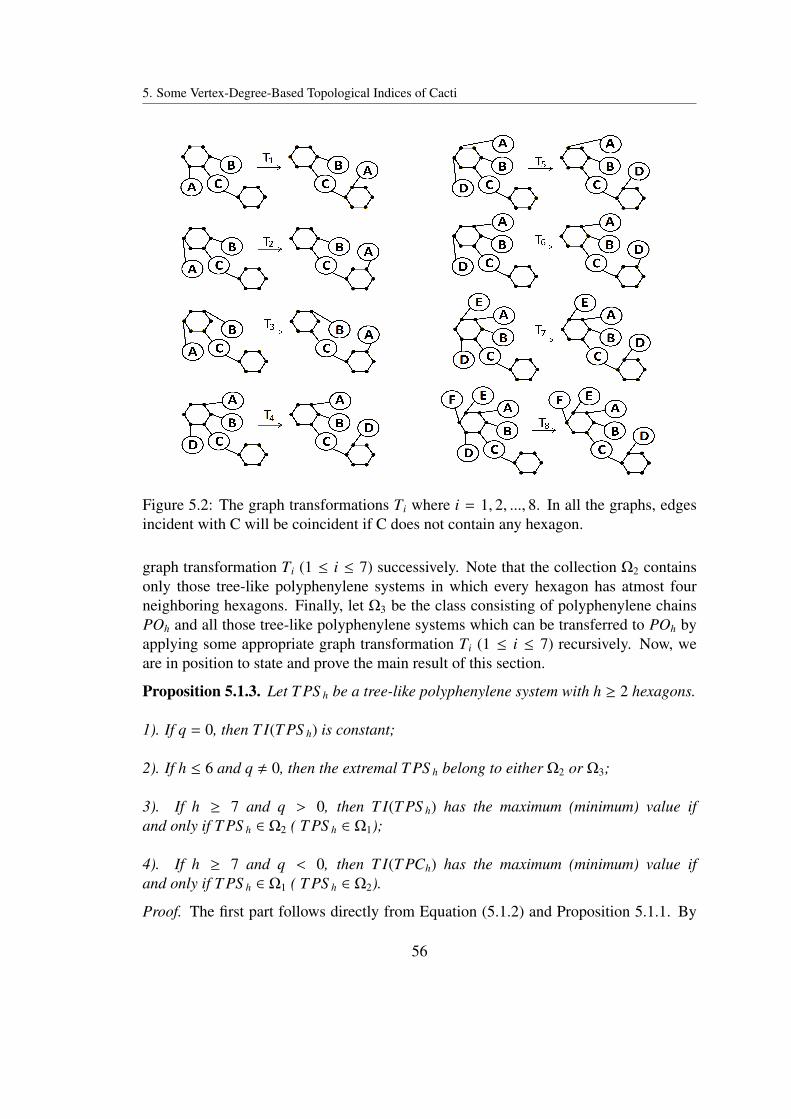
5. Some Vertex-Degree-Based Topological Indices of Cacti
Figure 5.2: The graph transformations Ti where i = 1, 2, ..., 8. In all the graphs, edgesincident with C will be coincident if C does not contain any hexagon.
graph transformation Ti (1 ≤ i ≤ 7) successively. Note that the collection Ω2 containsonly those tree-like polyphenylene systems in which every hexagon has atmost fourneighboring hexagons. Finally, let Ω3 be the class consisting of polyphenylene chainsPOh and all those tree-like polyphenylene systems which can be transferred to POh byapplying some appropriate graph transformation Ti (1 ≤ i ≤ 7) recursively. Now, weare in position to state and prove the main result of this section.
Proposition 5.1.3. Let T PS h be a tree-like polyphenylene system with h ≥ 2 hexagons.
1). If q = 0, then T I(T PS h) is constant;
2). If h ≤ 6 and q , 0, then the extremal T PS h belong to either Ω2 or Ω3;
3). If h ≥ 7 and q > 0, then T I(T PS h) has the maximum (minimum) value ifand only if T PS h ∈ Ω2 ( T PS h ∈ Ω1);
4). If h ≥ 7 and q < 0, then T I(T PCh) has the maximum (minimum) value ifand only if T PS h ∈ Ω1 ( T PS h ∈ Ω2).
Proof. The first part follows directly from Equation (5.1.2) and Proposition 5.1.1. By
56

5.1 Two Special Cacti: Tree-Like Polyphenylene and Spiro Hexagonal Systems
Figure 5.3: The tree-like polyphenylene system T PS ∗h′ where h′ = 2 + 5t1 and t1 ≥ 1.
using Propositions 5.1.1 and 5.1.2, one can easily obtained the second part. To provethe third part, let us consider the Equation (5.1.3). This equation implies that T I(T PS h)is maximum (respectively minimum) if and only if T I(PCh) is maximum (respectivelyminimum) and kq is minimum (respectively maximum) and hence from Proposition5.1.1 the desired result follows. The proof of fourth part is analogous to that of thirdpart.
All the terms defined for the tree-like polyphenylene systems can also be definedanalogously for the spiro hexagonal systems. It is easy to see that
x4,4(S Ch) = r, x2,4(S Ch) = 4(m + p + 1) + 2r, x2,2(S Ch) = 6h − 4(m + p + 1) − 3r,
where r,m and p is the number of ortho-hexagons, meta-hexagons and para-hexagonsrespectively in the spiro hexagonal chain S Ch. After substituting these values inEquation (3.1.1), one arrives at
T I(S Ch) = 6hθ2,2 + 4(θ2,4 − θ2,2)(m + p + 1) + (2θ2,4 − 3θ2,2 + θ4,4)r.
Since p + m + r = h − 2, the above equation can be rewritten as
T I(S Ch) = (2θ2,2 + 4θ2,4)h + 4(θ2,2 − θ2,4) + (θ2,2 − 2θ2,4 + θ4,4)r.
Let us denote by S C∗h the spiro hexagonal chain with r = 0. If S C1h and S C2
h are any twospiro hexagonal chains. Then
T I(S C1h) − T I(S C2
h) = (θ2,2 − 2θ2,4 + θ4,4)(r1 − r2),
where r1 and r2 are number of ortho-hexagons in S C1h and S C2
h respectively. Hence, wehave the following result.
57

5. Some Vertex-Degree-Based Topological Indices of Cacti
Proposition 5.1.4. Let S Ch be a spiro hexagonal chain with h ≥ 2 hexagons andsuppose that q′ = 2θ2,4 − θ2,2 − θ4,4.
1). If q′ < 0, then T I(S Ch) has the maximum (minimum) value if and only ifS Ch S Oh (S Ch S C∗h);
2). If q′ > 0, then T I(S Ch) has the maximum (minimum) value if and only ifS Ch S C∗h (S Ch S Oh);
3). If q′ = 0, then T I(S Ch) is constant.
Let T′
i (1 ≤ i ≤ 8) be the graph transformation obtained from Ti (1 ≤ i ≤ 7) by replacingthe tree-like polyphenylene systems (used in Ti) with the corresponding spiro hexagonalsystems. Moreover, let Ω
′
j (1 ≤ j ≤ 3) be the collection of all those spiro hexagonalsystems which correspond to the tree-like polyphenylene systems belonging to Ω j . Thefollowing result can be easily proved using the similar technique that has been used toprove the Proposition 5.1.3.
Proposition 5.1.5. Let S S h be a spiro hexagonal system with h ≥ 2 hexagons.
1). If q′ = 0, then T I(S S h) is constant;
2). If h ≤ 6 and q′ , 0, then the extremal S S h belong to either Ω′
2 or Ω′
3;
3). If h ≥ 7 and q′ > 0, then T I(S S h) has the maximum (minimum) value ifand only if S S h ∈ Ω
′
2 ( S S h ∈ Ω′
1);
4). If h ≥ 7 and q′ < 0, then T I(S S h) has the maximum (minimum) value ifand only if S S h ∈ Ω
′
1 ( S S h ∈ Ω′
2).
5.2 General Formulae for Calculating BID Indices ofPolyphenylene Dendrimer Nanostars
The dendrimer nanostars are highly branched macromolecules that appear to be photonfunnels just like artificial antennas. The step-wise growth of these macromoleculesfollows a mathematical progression and their size is in the nanometer scale. Detailsabout dendrimer nanostars and their applications can be found in (Newkome et al. 2002)and references cited therein.
In this section, we derive general formulae for calculating the BID indices of twopolyphenylene dendrimer nanostars (polyphenylene dendrimer nanostars are special
58

5.2 General Formulae for Calculating BID Indices of Polyphenylene Dendrimer Nanostars
types of dendrimer nanostars) whose molecular graphs are cacti. First, we consider themolecular graph NS 1[n] (see Figure 5.4) of the first type of polyphenylene dendrimernanostar where n denotes the steps of growth. Note that NS 1[n] has h1 = 3 × 2n − 2
Figure 5.4: The molecular graph NS 1[2] of the first type of polyphenylene dendrimernanostar with two generations.
hexagons. It is easy to see that NS 1[n] can be transformed into the polyphenylene chainPC∗h1
by repeating the graph transformation T3. Since the value of T I does not changeunder the graph transformation T3. Hence, by using the Equation (5.1.1) and definitionof PC∗h1
, one has the following result.
Proposition 5.2.1. For the dendrimer nanostar NS 1[n], the following formula holds:
T I(NS 1[n]) = (6θ2,2 + 12θ2,3 + 3θ3,3)2n − 12θ2,3 − 3θ3,3.
The following result is a direct consequence of Proposition 5.2.1:
Corollary 5.2.2. (Alikhani et al. 2014) The ABC index of the dendrimer nanostarNS 1[n] is given by
ABC(NS 1[n]) = (2 + 9√
2)2n − 6√
2 − 2.
Let us denote by NS 2[n] the molecular graph (see Figure 5.5) of the second type ofpolyphenylene dendrimer nanostar where n is the steps of growth. One can easily seethat NS 2[n] has h2 = 20 × 2n − 18 hexagons. Note that NS 2[n] can be transformed intothe polyphenylene chain PCh2 (in which r = h2−
∑ni=1 2i+1−2 = 16(2n−1)) by applying
some appropriate graph transformations Ti (1 ≤ i ≤ 7) successively. Recall that thegraph transformations Ti (1 ≤ i ≤ 7) does not change the value of T I. Hence, by usingthe Equation (5.1.1) and the definition of PCh2 , one has the following result.
Proposition 5.2.3. For the dendrimer nanostar NS 2[n], the following formula holds:
T I(NS 2[n]) = (14θ2,2 + 12θ2,3 + 9θ3,3)2n+2 − (48θ2,2 + 44θ2,3 + 35θ3,3).
59

5. Some Vertex-Degree-Based Topological Indices of Cacti
Figure 5.5: The molecular graph NS 2[2] of the second type of polyphenylene dendrimernanostar with two steps of growth.
The following corollaries are the direct consequence of Proposition 5.2.3.
Corollary 5.2.4. (Alikhani et al. 2014) The ABC index of the dendrimer nanostarNS 2[n] is given by
ABC(NS 2[n]) = 2[(
13√
2 + 6)
2n+1 −(23√
2 +353
)].
Corollary 5.2.5. (Rostami et al. 2012) The first geometric-arithmetic index, Randicindex and sum-connectivity index of the dendrimer nanostar NS 2[n] are given by
GA(NS 2[n]) =24√
65+ 23
2n+2 −88√
65+ 83
,R(NS 2[n]) =
(2√
6 + 10)
2n+2 − 22√
6 + 1073
,
χ(NS 2[n]) =
3√
32+
12√
5+ 7
2n+2 −(
35√
6+
44√
5+ 24
).
60

5.3 Extremal General Cacti for Some Vertex-Degree-Based Topological Indices
5.3 Extremal General Cacti for Some Vertex-Degree-Based Topological Indices
Let Cn,k be the collection of all cacti with k cycles and n ≥ 5 vertices and denote byC∗n,k the sub-collection of Cn,k containing those cacti in which all the pendant verticesare adjacent with the same vertex. Let G0(n, k) ∈ C∗n,k and is obtained from the star S n
by adding k mutually independent edges (see Figure 5.6). Take F1(n, k) = 16k(n − 1)2
Figure 5.6: The cactus G0(n, k).
and F2(n, k) = 16k(n − 1)n−1. Firstly, we will prove the extremal results for the firstmultiplicative Zagreb index Π1 and second multiplicative Zagreb index Π2. For this, weneed some lemmas.
Lemma 5.3.1. (Gutman 2011; Xu and Hua 2012) If G ∈ Cn,0, then
Π1(G) ≥ F1(n, 0) and Π2(G) ≤ F2(n, 0)
with equalities if and only if G G0(n, 0).
Lemma 5.3.2. (Xu and Hua 2012) Let G ∈ Cn,1. Then
Π1(G) ≥ F1(n, 1) and Π2(G) ≤ F2(n, 1),
with equalities if and only if G G0(n, 1).
Transformation A. (Deng 2007; Xu and Hua 2012) Let G is a connected graph anduv ∈ E(G) such that dv ≥ 2, NG(u) = v,w1,w2, ...,ws where w1,w2, ...,ws are pendentvertices. Let G′ = G − uw1, uw2, ..., uws + vw1, vw2, ..., vws. For the figures of G andG′, see (Deng 2007; Xu and Hua 2012).
61
5. Some Vertex-Degree-Based Topological Indices of Cacti
Lemma 5.3.3. (Xu and Hua 2012) For the graphs G and G′ given in the definition ofthe Transformation A,
Π1(G) > Π1(G′) and Π2(G) < Π2(G′).
Transformation B. (Deng 2007; Xu and Hua 2012) Let u and v are two vertices in aconnected graph G such that the pendent vertices u1, u2, ..., ur are adjacent with u andthe pendent vertices v1, v2, ..., vt are adjacent with v. Let G′ = G − uu1, uu2, ..., uur +vu1, vu2, ..., vur and G′′ = G− vv1, vv2, ..., vvt+ uv1, uv2, ..., uvt. For the figures of G,G′ and G′′, see (Deng 2007; Xu and Hua 2012).
Lemma 5.3.4. (Xu and Hua 2012) For the graphs G, G′ and G′′ given in the definitionof the Transformation B,
Π1(G) > Π1(G′) or Π1(G) > Π1(G′′),
and Π2(G) < Π2(G′) or Π2(G) < Π2(G′′).
Remark 5.3.5. By repeating the Transformation A and Transformation B, any cactusG1 ∈ Cn,k can be transferred into a cactus G2 ∈ C∗n,k. By Lemma 5.3.3 and Lemma 5.3.4,Π1(G1) ≥ Π1(G2) and Π2(G1) ≤ Π2(G2).
Lemma 5.3.6. If f (x) = xx(x − 2)2−x, then f (x) is increasing for x ≥ 3.
Proof. After simple calculations, one has f ′(x) = f (x)ln(
xx−2
)which is obviously
positive for x ≥ 3.
Now, we are in position to state and prove the first main result of this section.
Theorem 5.3.7. Let G is any cactus belongs to the collection Cn,k. Then
Π1(G) ≥ F1(n, k) and Π2(G) ≤ F2(n, k),
with equalities if and only if G G0(n, k)
Proof. Bearing in mind the Remark 5.3.5, it is sufficient to take G from the collectionC∗n,k. The theorem will be proved by induction on n + k. For k = 0, 1, the theoremdirectly follows from Lemma 5.3.1 and Lemma 5.3.2. Let us suppose that k ≥ 2, thenthere exist three vertices u, v and w on some cycle of G such that u is adjacent with boththe vertices v,w, du = dv = 2 and dw = x ≥ 3. There are two possibilities:
62

5.3 Extremal General Cacti for Some Vertex-Degree-Based Topological Indices
Case 1. If there is no edge between v and w. Then the graph G′ = G− u+ vw belongs tothe collection C∗n−1,k. Hence, by using the inductive hypothesis and the condition n ≥ 5,one has
Π1(G) = 4 × Π1(G′) ≥ 4 × F1(n − 1, k) = 4(n − 2n − 1
)2
F1(n, k) > F1(n, k).
Π2(G) = 4 × Π2(G′) ≤ 4 × F2(n − 1, k) =4(n − 2)n−2
(n − 1)n−1 F2(n, k) < F2(n, k).
Case 2. If there is an edge between v and w. Note that the graph G′ = G − u− v belongsto the collection C∗n−2,k−1. Let NG(w) = u, v, u1, u2, ..., ux−2. By using the inductivehypothesis and the fact that the function f (x) = 16x2
(x−2)2 is decreasing for 3 ≤ x ≤ n − 1,one has
Π1(G) =16x2
(x − 2)2Π1(G′) ≥ 16(n − 1)2
(n − 3)2 F1(n − 2, k − 1) = F1(n, k).
The equality Π1(G) = F1(n, k) holds if and only if G′ G0(n − 2, k − 1) and x = n − 1.For the Π2, bearing in mind the inductive hypothesis and Lemma 5.3.6, one has
Π2(G) = 16x2Π2(G′)
x−2∏i=1
xdui
x−2∏i=1
(x − 2)dui
≤ 16xx(x − 2)2−xF2(n − 2, k − 1)
≤ 16(n − 1)n−1(n − 3)3−nF2(n − 2, k − 1) = F2(n, k).
The equality Π2(G) = F2(n, k) holds if and only if G′ G0(n − 2, k − 1) and x = n − 1.This completes the proof.
The following corollary about the NK index is a direct consequence of Theorem 5.3.7.
Corollary 5.3.8. Let G is any cactus belongs to the collection Cn,k. Then
NK(G) ≥ 4k(n − 1)
with equality if and only if G G0(n, k).
Now, let us prove the extremal results for the modified first multiplicative Zagreb indexΠ∗1, modified second Zagreb index M∗2, Albertson index A, harmonic index H and zeroth-order general Randic index 0Rα. To proceed, we need some preparation. Let F3(n, k) =
63

5. Some Vertex-Degree-Based Topological Indices of Cacti
4knn−2k−1(n + 1)2k, F4(n, k) = 1 + k4 −
kn−1 , F5(n, k) = n(n − 3) − 2(k − 1), F6(n, k) =
4kn+1 +
2(n−2k−1)n + k
2 and ψ(n, k) = (n − 1)[(n − 1)α−1 + 1
]+ 2k(2α − 1).
Lemma 5.3.9. Let G ∈ Cn,0. Then
Π∗1(G) ≤ F3(n, 0), see (Xu and Das 2012)
M∗2(G) ≥ F4(n, 0), see (Hu et al. 2004)
A(G) ≤ F5(n, 0), see (Tavakoli et al. 2014)
H(G) ≥ F6(n, 0). see (Zhong 2012a)
The equality holds in each of the above inequalities if and only if G G0(n, 0).
Lemma 5.3.10. If G ∈ Cn,1, then
Π∗1(G) ≤ F3(n, 1), see (Xu and Das 2012)
M∗2(G) ≥ F4(n, 1), see (Wu and Zhang 2005)
A(G) ≤ F5(n, 1)), see (Hansen and Melot 2005)
H(G) ≥ F6(n, 1). see (Zhong 2012b)
The equality holds in each of the above inequalities if and only if G G0(n, 1).
Lemma 5.3.11. Let f (x) = (x+1)p(
x+2x−p+2
)x−pwhere x > p ≥ 1. Then f (x) is increasing
for x ≥ 2.
Proof. By simple calculations, one has
f ′(x) = f (x)(ln
(x + 2
x
)+
p(3x − p + 4)(x + 1)(x + 2)(x + 2 − p)
)which is positive for x ≥ 2 and hence the lemma follows.
Lemma 5.3.12. If f (x) = px+1 +
(x−p)x+2 −
(x−p)x−p+2 where x > p ≥ 1. Then f (x) is decreasing
for x ≥ 2.
Proof. After simple calculations, one has
f ′(x) = p(
1(x + 2)2 −
1(x + 1)2
)+ 2
(1
(x + 2)2 −1
(x + 2 − p)2
)< 0
Lemma 5.3.13. The function f (x) = x2−x(x + 2)x is increasing for x ≥ 3.
64

5.3 Extremal General Cacti for Some Vertex-Degree-Based Topological Indices
Proof. The proof is straight forward.
Lemma 5.3.14. If f (x) = 12 +
2xx+2 −
2(x−2)x , then f (x) is decreasing for x ≥ 3.
Proof. The proof is trivial.
Lemma 5.3.15. (Hu et al. 2007) If T is a tree with n vertices, then
0Rα(T )
≤ ψ(n, 0) if α < 0 or α > 1≥ ψ(n, 0) if 0 < α < 1,
with equalities if and only if G G0(n, 0).
Let us denote by (G1, u) and (G2, v) the graphs rooted at u and v respectively. LetG = (G1, u) (G2, v) be the graph obtained from (G1, u) and (G2, v) by identifying uwith v.
Theorem 5.3.16. (Hua and Deng 2007) If G is the unicyclic graph with n vertices andcontains the cycle of length l, then
0Rα(G)
≤ (n − l + 2)α + (l − 1)2α + n − l if α < 0 or α > 1≥ (n − l + 2)α + (l − 1)2α + n − l if 0 < α < 1,
with equalities if and only if G G = (Cl, u) (S n−l+1, v).
The following corollary is an immediate consequence of Theorem 5.3.16.
Corollary 5.3.17. Let G be any unicyclic graph with n vertices. Then
0Rα(G)
≤ ψ(n, 1) if α < 0 or α > 1≥ ψ(n, 1) if 0 < α < 1,
with equalities if and only if G G0(n, 1).
Proof. Let us take f (l) = (n − l + 2)α + (l − 1)2α + n − l where 3 ≤ l ≤ n. Then aftersimple calculations, one has f ′(l) = α(1 − α)(n − l + 2 − Θ1)Θα−2
2 where 1 < Θ1 < 2and Θ1 < Θ2 < n − l + 2. Note that f ′(l) is positive (respectively negative) for 0 <α < 1 (respectively for α < 0 or α > 1). Hence, f (l) attains its minimum (respectivelymaximum) value at l = 3 for 0 < α < 1 (respectively for α < 0 or α > 1). Therefore,from Theorem 5.3.16, desired result follows.
Lemma 5.3.18. Let f (x) = xα − (x − p)α, where x > p ≥ 1. Then f (x) is decreasing(respectively increasing) for 0 < α < 1 (respectively for α < 0 or α > 1).
65

5. Some Vertex-Degree-Based Topological Indices of Cacti
Proof. Note that f ′(x) = pα(α − 1)Θα−2 where x − p < Θ < x. It can be easily seenthat f ′(x) is negative (respectively positive) for 0 < α < 1 (respectively for α < 0 orα > 1).
Now, we are ready to prove the extremal results for the Π∗1,M∗2, A,H and 0Rα indices.
Theorem 5.3.19. Let G be any cactus belongs to the collection Cn,k. Then
Π∗1(G) ≤ F3(n, k), M∗2(G) ≥ F4(n, k), A(G) ≤ F5(n, k), H(G) ≥ F6(n, k) and
0Rα(G)
≤ ψ(n, k) if α < 0 or α > 1,≥ ψ(n, k) if 0 < α < 1.
The equality in each inequality holds if and only if G G0(n, k).
Proof. We will prove the theorem by using induction on n+ k. For k = 0, 1, the theoremdirectly follows from Lemma 5.3.9, Lemma 5.3.10, Lemma 5.3.15 and Corollary 5.3.17.If k ≥ 2, then for n = 5 there is only one cactus which is isomorphic to G0(5, 2) andhence the theorem holds in this case. Let us assume that G ∈ Cn,k where k ≥ 2 andn ≥ 6. Then there are two possibilities:
Case 1. If G has atleast one pendent vertex. Let u0 be the pendent vertex adjacent with vand dv = x. Let NG(v) = u0, u1, u2, ..., ux−1. Without loss of generality one can assumethat dui = 1 for 0 ≤ i ≤ p− 1 and dui ≥ 2 for p ≤ i ≤ x− 1. Let G′ be the graph obtainedfrom G by removing the pendent vertices u0, u1, u2, ..., up−1, then G′ ∈ Cn−p,k and henceone has
Π∗1(G) = (x + 1)p × Π∗1(G′)
x−1∏i=p
(x + dui)
x−1∏i=p
(x − p + dui)
≤ F3(n − p, k)(x + 1)p
×x−1∏i=p
(x + dui
x − p + dui
)(by inductive hypothesis)
≤ F3(n − p, k)(x + 1)p
(x + 2
x − p + 2
)x−p
(since dui ≥ 2 for i ≥ p)
≤ F3(n, k)((n + 1)(n − p)n(n + 1 − p)
)n−2k−p−1
(by Lemma 5.3.11)
≤ F3(n, k).
66

5.3 Extremal General Cacti for Some Vertex-Degree-Based Topological Indices
The equality Π∗1(G) = F3(n, k) holds if and only if G′ G0(n − p, k), x = n − 1 andn − 2k − p − 1 = 0.
M∗2(G) − F4(n, k) = M∗2(G′) +px+
x−1∑i=p
1xdui
−x−1∑i=p
1(x − p)dui
− F4(n, k)
≥ F4(n − p, k) +px− p
x(x − p)
x−1∑i=p
1dui
− F4(n, k)
≥ pn − 1
(12− k
n − p − 1
)≥ 0. (since 2k ≤ n − p − 1)
The second last inequality holds because dui ≥ 2 for p ≤ i ≤ x − 1 and x ≤ n − 1. Notethat the equality M∗2(G) − F4(n, k) = 0 holds if and only if G′ G0(n − p, k), x = n − 1and 2k = n − p − 1.
A(G) − F5(n, k) = A(G′) + p(x − 1) − F5(n, k)
+
x−1∑i=p
(| x − dui | − | x − p − dui |)
≤ F5(n − p, k) − F5(n, k) + p(x − 1) + p(x − p)≤ 0.
We have used the fact | x−p−dui+p | ≤ | x−p−dui | + p. The equality A(G)−F5(n, k) = 0holds if and only if G′ G0(n − p, k) and x = n − 1.
H(G) − F6(n, k) = H(G′) +2p
x + 1− F6(n, k)
+
x−1∑i=p
(2
x + dui
− 2x − p + dui
)≥ F6(n − p, k) − F6(n, k) +
2px + 1
+2(x − p)
x + 2− 2(x − p)
x − p + 2
≥ 2p(n − p − 2k − 1)(2n − p + 1)n(n − p)(n − p + 1)(n + 1)
≥ 0.
The second last inequality follows from Lemma 5.3.12 and the last inequality holdsbecause n− p− 2k − 1 ≥ 0. Note that the equality H(G)− F6(n, k) = 0 holds if and only
67

5. Some Vertex-Degree-Based Topological Indices of Cacti
if G′ G0(n − p, k), x = n − 1 and n − p − 2k − 1 = 0. Finally for 0Rα, one has
0Rα(G) = 0Rα(G′) + p + xα − (x − p)α.
From inductive hypothesis, it follows that
0Rα(G) − ψ(n, k)
≤ (n − p − 1)α − (n − 1)α + xα − (x − p)α if α < 0 or α > 1≥ (n − p − 1)α − (n − 1)α + xα − (x − p)α if 0 < α < 1,
with equalities if and only if G′ G0(n − p, k). By using Lemma 5.3.18, one has
0Rα(G) − ψ(n, k)
≤ 0 if α < 0 or α > 1≥ 0 if 0 < α < 1,
with equalities if and only if G′ G0(n − p, k) and x = n − 1.
Case 2. If G does not contain any pendent vertex. Then there exist three vertices u, vand w on some cycle of G such that u is adjacent with both the vertices v,w, du = dv = 2and dw = x ≥ 3. Then there are two further possibilities:
Subcase 2.1. If there is no edge between v and w. Then note that the graph G′ =G − u + vw belongs to the collection Cn−1,k and hence one has
Π∗1(G) = 4 × Π∗1(G′) ≤ 4 × F3(n − 1, k)
= F3(n, k)(4n2r(n − 1)n−2r−2
(n + 1)2rnn−2r−1
)< F3(n, k)
( nn + 1
)2r(n − 1
n
)n−2r−1
(since n − 1 > 4)
< F3(n, k).
M∗2(G) − F4(n, k) = M∗2(G′) +14− F4(n, k) ≥ F4(n − 1, k) +
14− F4(n, k)
=14− k
(n − 2)(n − 1)>
14− k
2(n − 1)
≥ 0. (since k ≤ n − 12
)
A(G) − F5(n, k) = A(G′) − F5(n, k) ≤ F5(n − 1, k) − F5(n, k) < 0.
68

5.3 Extremal General Cacti for Some Vertex-Degree-Based Topological Indices
H(G) − F6(n, k) = H(G′) +24− F6(n, k) > F6(n − 1, k) − F6(n, k) +
2n
=4k
n(n + 1)+
2(n − 2k − 2)n(n − 1)
≥ 2(3n − 5)n(n − 1)(n + 1)
> 0.
We have used the facts n > 4, k ≥ 2 and n − 1 ≥ 2k to establish the inequality H(G) −F6(n, k) > 0. For the 0Rα, we have
0Rα(G) = 0Rα(G′) + 2α.
By using inductive hypothesis, one has
0Rα(G) − ψ(n, k)
≤ 2α − 1 − [(n − 1)α − (n − 2)α] if α < 0 or α > 1≥ 2α − 1 − [(n − 1)α − (n − 2)α] if 0 < α < 1,
with equalities if and only if G′ G0(n − 1, k). But, on the other hand, one has
2α − 1 − [(n − 1)α − (n − 2)α] = α(Θα−11 − Θα−1
2 )
< 0 if α < 0 or α > 1> 0 if 0 < α < 1,
where 1 < Θ1 < 2, n − 2 < Θ2 < n − 1.
Subcase 2.2. If there is an edge between v and w. Note that the graph G′ = G − u − vbelongs to the collection Cn−2,k−1. Let NG(w) = u, v, u1, u2, ..., ux−2. Then one has
Π∗1(G) = 4(x + 2)2 × Π∗1(G′)
x−2∏i=1
(x + dui)
x−2∏i=1
(x − 2 + dui)
≤ F3(n − 2, k − 1) × 4(x + 2)2
x−2∏i=1
(x + dui
x − 2 + dui
)≤ F3(n − 2, k − 1) × 4(x + 2)2
(x + 2
x
)x−2
(as dui ≥ 2 for all i)
≤ F3(n, k)((n + 1)(n − 2)
n(n − 1)
)n−2k−1
(by Lemma 5.3.13)
≤ F3(n, k) (since 2k ≤ n − 1).
The equality Π∗1(G) = F3(n, k) holds if and only if G′ G0(n − 2, k − 1), x = n − 1 and
69

5. Some Vertex-Degree-Based Topological Indices of Cacti
n − 2k − 1 = 0.
M∗2(G) − F4(n, k) = M∗2(G′) +14+
1x− F4(n, k)
+
x−2∑i=1
1xdui
−x−2∑i=1
1(x − 2)dui
≥ F4(n − 2, k − 1) − F4(n, k) +14+
1x
− 2x(x − 2)
x−2∑i=1
1dui
≥ n − 2k − 1(n − 3)(n − 1)
(since dui ≥ 2 for all i)
≥ 0. (since 2k ≤ n − 1)
The equality M∗2(G) − F4(n, k) = 0 holds if and only if G′ G0(n − p, k), x = n − 1 and2k = n − 1.
A(G) − F5(n, k) = A(G′) + 2(x − 2) − F5(n, k)
+
x−2∑i=1
(| x − dui | − | x − 2 − dui |)
≤ F5(n − 2, k − 1) − F5(n, k) + 4(x − 2)≤ 0.
We have used the fact | x − 2 − dui + 2 | ≤ | x − 2 − dui | +2 to prove the inequalityA(G) − F5(n, k) ≤ 0. The equality A(G) − F5(n, k) = 0 holds if and only if G′ G0(n − 2, k − 1) and x = n − 1.
H(G) − F6(n, k) = H(G′) − F6(n, k) +4
x + 2+
12
+
x−2∑i=1
(2
x + dui
− 2x − 2 + dui
)≥ F6(n − 2, k − 1) − F6(n, k) +
12+
2xx + 2
− 2(x − 2)x
(since dui ≥ 2 for all i)
≥ 4(n − 2k − 1)(2n − 1)n(n − 2)(n − 1)(n + 1)
(by Lemma 5.3.14)
≥ 0.
70
5.3 Extremal General Cacti for Some Vertex-Degree-Based Topological Indices
The equality H(G) − F6(n, k) = 0 holds if and only if G′ G0(n − 2, k − 1), x = n − 1and 2k = n − 1. Lastly, for the 0Rα, one has
0Rα(G) = 0Rα(G′) + 2α+1 + xα + (x − 2)α.
From inductive hypothesis, it follows that
0Rα(G) − ψ(n, k)
≤ (n − 3)α − (n − 1)α + xα − (x − 2)α if α < 0 or α > 1≥ (n − 3)α − (n − 1)α + xα − (x − 2)α if 0 < α < 1,
with equalities if and only if G′ G0(n − 2, k − 1). By using Lemma 5.3.18, one has
0Rα(G) − ψ(n, k)
≤ 0 if α < 0 or α > 1≥ 0 if 0 < α < 1,
with equalities if and only if G′ G0(n − 2, k − 1) and x = n − 1. This completes theproof.
71

5. Some Vertex-Degree-Based Topological Indices of Cacti
72

Chapter 6On the ABC index and AZI
Recently Gutman and Tosovic (2013) tested the correlation abilities of twenty vertex-degree-based topological indices for the case of standard heats of formation and normalboiling points of octane isomers and they found that the AZI (respectively ABC index)yields the best (respectively second-best) results. In this chapter some mathematicalproperties of these indices are explored.
6.1 The ABC IndexDas and Trinajstic (2010) showed that ABC index is less than GA index for allthose graphs (except K1,4 and T ∗, see Figure 6.1) in which the difference between themaximum and minimum degree is less than or equal to 3. In this section, it is proved
Figure 6.1: The molecular graphs K1,4 and T ∗
that ABC index remains lesser than GA index for line graphs of molecular graphs, forgeneral graphs in which the difference between the maximum and minimum degree isless than or equal to (2δ − 1)2 (where δ is the minimum degree and δ ≥ 2) and for somefamilies of trees. Furthermore, a sharp lower and upper bound for the ABC index interms of GA index is also derived here.
If the graph G has s ≥ 2 components G1,G2, . . . ,Gs, then from the definition of the GAand ABC indices it follows that ABC(G) =
∑si=1 ABC(Gi) and GA(G) =
∑si=1 GA(Gi).
73
6. On the ABC index and AZI
Moreover, if the graph G is trivial then ABC(G) = GA(G) = 0 = ABC(P2). Hence,we restrict our considerations to only non-trivial and connected graphs. Let T ∗ be thetree with eight vertices, obtained by joining the central vertices of two copies K1,3 by anedge (see Figure 6.1). To prove the first main theorem of this section, we need followingknown result.
Theorem 6.1.1. (Das and Trinajstic 2010) Let G be a non-trivial and connected graphwith the maximum degree ∆ and the minimum degree δ. If ∆ − δ ≤ 3 and G K1,4,T ∗,then GA(G) > ABC(G).
In the following theorem, we compare the GA index and the ABC index for line graphof a molecular graph.
Theorem 6.1.2. Let M be a molecular (connected) graph with n ≥ 3 vertices andG L(M). Then GA(G) > ABC(G).
Proof. If n ≤ 4 or M Pn, then it can be easily seen that G is a molecular graph whichsatisfies the hypothesis of Theorem 6.1.1 and hence the result follows. Let us assumethat n ≥ 5 and M Pn. Note that 1 ≤ di ≤ 6 for all vertices vi of G. Hence, the possibledegree pairs of edges of G are: (6, 6), (6, 5), (6, 4), (6, 3), (6, 2), (6, 1), (5, 5), (5, 4), (5, 3),(5, 2), (5, 1), (4, 4), (4, 3), (4, 2), (4, 1), (3, 3), (3, 2), (3, 1), (2, 2), (2, 1). The values of
θi j =2√
did j
di+d jand ϕi j =
√di+d j−2
did jfor all above mentioned degree pairs are given in the
Table 5.1 and Table 5.2 (Table 5.2 is taken from (Das and Trinajstic 2010)). From thesetables one can note easily that
θi j − ϕi j
≥ 2√
67 −
√56 ≈ −0.2130 if (di, d j) = (4, 1), (5, 1), (6, 1)
≈ 0.0495 if (di, d j) = (3, 1)≈ 0.1589 if (di, d j) = (6, 2)≈ 0.1964 if (di, d j) = (5, 2)≈ 0.2357 if (di, d j) = (2, 1), (4, 2)≥ 2
√6
5 −1√2≈ 0.2727 otherwise
(6.1.1)
It is claimed that6∑
b=2
x1,b(G) ≤ ⌊|V(G)|2⌋ ≤ ⌊ |E(G)|
2⌋. (6.1.2)
The right inequality obviously holds because G contains at least one cycle. To provethe left inequality it is enough to show that no two pendent edges of G are adjacent.Contrarily, suppose that e1 = uv and e2 = uw are pendent edges of G. Since n ≥ 5, orderof G is at least 4. This implies that there exists a vertex t (different from v,w) adjacent
74

6.1 The ABC Index
with u in G. Then the graph obtained by removing all vertices except u, v,w, t of G isK1,3 , a contradiction to Lemma 2.9.1. Now, we consider two cases:
Case 1. If x1,b(G) = 0 for all b ≥ 4, then it follows from (6.1.1) that θi j − ϕi j > 0 for alledges viv j ∈ E(G) and hence GA(G) > ABC(G).
Case 2. If x1,b(G) = 0 not for all b ≥ 4.If x2,5(G) = x2,6(G) = 0, then from (6.1.1) and (6.1.2), it follows that
GA(G) − ABC(G) =∑
viv j∈E(G)
(θi j − ϕi j) > 0 (6.1.3)
(di, d j) (6,6) (6,5) (6,4) (6,3) (6,2) (6,1) (5,5) (5,4) (5,3) (5,2) (5,1)θi j 1 2
√30
112√
65
2√
23
√3
22√
67 1 4
√5
9
√154
2√
107
√5
3
ϕi j13
√52
√310
1√3
13
√72
1√2
√56
2√
25
12
√75
√25
1√2
2√5
Table 6.1: The values of θi j and ϕi j for all edges with degrees (di, d j) where 5 ≤ di ≤ 6and di ≥ d j
(di, d j) (4,4) (4,3) (4,2) (4,1) (3,3) (3,2) (3,1) (2,2) (2,1)θi j 1 4
√3
72√
23 0.8 1 2
√6
5
√3
2 1 2√
23
ϕi j12
√32
12
√53
1√2
√3
223
1√2
√23
1√2
1√2
Table 6.2: The values of θi j and ϕi j for all edges with degrees (di, d j) where 2 ≤ di ≤ 4and di ≥ d j
If at least one of x2,5(G), x2,6(G) is nonzero. Consider the edge e = xy ∈ E(G) wheredegree of x and y is two and c (c = 5, 6) respectively. Let l denote number of verticesof degree two which are adjacent with y. Then 1 ≤ l ≤ 2 for otherwise K1,3 wouldbe an induced subgraph of G. Note that the vertex y lies on either of the cliquesKc−1,Kc of G and hence the edges with possible degree pairs of these cliques in Gare (6, 6), (6, 5), (6, 4), (6, 3), (5, 5), (5, 4), (5, 3), (4, 4), (4, 3), (3, 3). For all these degreepairs θi j − ϕi j ≥ 0.2727. Moreover, corresponding to every clique Kd (d = 4, 5, 6) of G,there exist at most 2d edges with degree pairs (2, c) in G, where vertex of degree c (thatis y) lies on Kd. Since the size of Kd is d(d−1)
2 ≥ 2d for d ≥ 5. Therefore, if G does nothave clique K4, then by using (6.1.1) and (6.1.2) one can easily see that the inequality(6.1.3) holds. If G has clique K4. It can be easily seen that no edge with degree pairs(2, 6) can be incident with any vertex of the clique K4. This implies, corresponding to
75

6. On the ABC index and AZI
every clique K4 there exist at most 8 edges with degree pairs (2, 5), but the size of K4 is6. Hence,
8(0.1964) + 6(0.2727)14
≈ 0.2291 > 0.2130.
This completes the proof.
Now, we prove that conclusion of Theorem 6.1.1 remains true if the minimum degreeis k ≥ 2 and the difference between the maximum and minimum degree is less than orequal to (2k − 1)2. To proceed, we need the following lemma:
Lemma 6.1.3. If f (x, y) = (x + y)2x2 − (x + y2 )2(2x + y − 2) , k ≤ x ≤ k + (2k − 1)2 and
0 ≤ y ≤ (2k − 1)2 where k ≥ 2 then f (x, y) > 0.
Proof. Step 1. If we take x = k, then
g(y) = f (k, y) = (k + y)2k2 − (k +y2
)2(2k + y − 2)
and g′(y) > 0 implies that α < y < β, where
α =23
(1 − 3k + 2k2) − 23
√1 + 4k2 − 6k3 + 4k4
andβ =
23
(1 − 3k + 2k2) +23
√1 + 4k2 − 6k3 + 4k4.
It means that g is increasing in the interval (α, β) and decreasing in the intervals (−∞, α)and (β,∞). Since α < 0 < β < (2k − 1)2, so g is increasing in (0, β) and decreasing in(β, (2k−1)2). Moreover, g(0) = k2k2−2(k−1) > 0 and g((2k−1)2) = k4+k2− k
2+14 > 0.
It follows that g(y) > 0 for all y ∈ [0, (2k − 1)2].
Step 2. Now we take y = y0, where y0 is any fixed integer in the interval [0, (2k − 1)2].If h(x) = f (x, y0) then
h′(x) = (2x + y0)[(2x2 + 2 − 3x) +
(2x − 3
2
)y0
]> 0
for all x ≥ k ≥ 2. Hence, h(x) = f (x, y0) is increasing in [k,∞). Combining both theresults proved in Step 1 and Step 2, we have Lemma.
Theorem 6.1.4. Let G be a connected graph with the maximum degree ∆ and theminimum degree δ ≥ 2. If ∆ − δ ≤ (2δ − 1)2 then GA(G) > ABC(G).
Proof. Let us consider the quantity
Γ = d2i d2
j −14
(di + d j)2(di + d j − 2), (6.1.4)
76

6.1 The ABC Index
where di and d j are the degrees of vertices vi and v j respectively in G. Since δ ≤ di, d j ≤∆ ≤ δ + (2δ − 1)2 this implies that | di − d j |≤ (2δ − 1)2. Without loss of generality wecan suppose that di ≥ d j then di = d j + θ for some θ ; 0 ≤ θ ≤ (2δ − 1)2 and Equation(6.1.4) becomes
Γ =(d j + θ
)2d2
j −(d j +
θ
2
)2
(2d j + θ − 2), (6.1.5)
where δ ≤ d j ≤ δ + (2δ − 1)2 and 0 ≤ θ ≤ (2δ − 1)2. Now, from Lemma 6.1.3 andEquation (6.1.5), we have the desired result.
If the condition ∆− δ ≤ (2δ− 1)2 is replaced by ∆− δ ≤ (2δ− 1)2 + 1 in Theorem 6.1.4,then the conclusion may not be true. For instance, consider the complete bipartite graphKr,s, if we take r = δ ≥ 2 and s = (2δ − 1)2 + δ + 1 then
GA(Kr,s) =2[δ((2δ − 1)2 + δ + 1)
] 32
(2δ − 1)2 + 2δ + 1
<√δ((2δ − 1)2 + 2δ − 1)((2δ − 1)2 + δ + 1) = ABC(Kr,s).
On the other hand, consider the graph G obtained by joining any vertex of K12 to avertex of K3 by an edge. Then ∆ = 12, δ = 2 which means that ∆− δ = 10 > (2(2)− 1)2,but GA(G) > ABC(G). We have the following result:
Theorem 6.1.5. If G is a connected graph with the minimum degree δ ≥ 2 and |di−d j| ≤(2δ − 1)2 for all edges viv j ∈ E(G), then GA(G) > ABC(G).
Proof. The proof is similar to the proof of Theorem 6.1.4 and hence is omitted.
A stronger version of the above result can be analogously proved:
Theorem 6.1.6. Let G be a connected graph with the minimum degree δ ≥ 2 and |di −d j| ≤ (2k − 1)2 for all viv j ∈ E(G), where k = mindi, d j. Then GA(G) > ABC(G).
Let δ1 be the minimum non-pendant vertex degree in G. Now, we compare GA indexand ABC index for trees.
Theorem 6.1.7. If T is a tree with n ≥ 3 vertices such that x1,b(T ) = 0 for all b ≥ 4 and∆ − δ1 ≤ (2δ1 − 1)2, then GA(T ) > ABC(T ).
Proof. Let us consider the difference
GA(T ) − ABC(T ) =∑
viv j∈E(T )
(θi j − ϕi j)
=∑
viv j∈E(T ),di,1,d j
(θi j − ϕi j) +∑
viv j∈E(T ),di=1 or d j=1
(θi j − ϕi j).
77
6. On the ABC index and AZI
As x1,b(T ) = 0 for all b ≥ 4, from (6.1.1) it follows that∑viv j∈E(T ),
di=1 or d j=1
(θi j − ϕi j) > 0
Now, we have to prove that ∑viv j∈E(T ),di,1,d j
(θi j − ϕi j) > 0
To do so, let di, d j ≥ 2 then using the same technique, adopted in the proof of Theorem6.1.4, we have
d2i d2
j −14
(di + d j)2(di + d j − 2) > 0
which is equivalent to2√
did j
di + d j>
√di + d j − 2
did j
which implies that ∑viv j∈E(T ),di,1,d j
2√
did j
di + d j−
√di + d j − 2
did j
> 0.
This completes the proof.
Now, for Starlike tree, we have the following result.
Theorem 6.1.8. Let S = S (r1, r2, ..., rk) be a Starlike tree.
1). If ri ≥ 4 for all i, then GA(S ) > ABC(S );
2). If ri ≥ 2 for all i and
k∑i=1
ri
k ≥ 4, then GA(S ) > ABC(S );
3). If
k∑i=1
ri
k ≥ 8, then GA(S ) > ABC(S ).
Proof. 1). The edges of S with possible degree pairs are: (2, 1), (2, 2), (k, 2). FromTable 2 we have
θi j − ϕi j ≈0.2357 if (di, d j) = (2, 1)
0.2929 if (di, d j) = (2, 2)(6.1.6)
Moreover, the function f (k) = θ2k − ϕ2k =(
2√
2kk+2 −
1√2
)is decreasing in (2,∞) and
f (k) → − 1√2≈ −0.7071 when k → ∞. Hence, we have f (k) > − 1√
2≈ −0.7071 for all
78

6.1 The ABC Index
k. Since ri ≥ 4 for all i, this implies that there are k edges with degree pairs (1, 2), kedges with degree pairs (2, k) and at least 2k edges with degree pairs (2, 2) in S . Thiscompletes the proof of first part.
Note that2√
did j
di+d j−
√di+d j−2
did j> −1 if (di, d j) = (1, k) for all k. Using the same technique
as adopted in the proof of the first part, one can easily prove the remaining parts.
In the following theorem, we establish sharp lower and upper bounds for ABC index interms of GA index:
Theorem 6.1.9. Let G be a connected graph having n ≥ 3 vertices with the minimumdegree δ ≥ 2, then
√2(n − 2)n − 1
GA(G) ≤ ABC(G) ≤ n + 1
4√
n − 1GA(G) (6.1.7)
with left equality if and only if G Kn and right equality if and only if G C3.
Proof. Suppose that 2 ≤ d j ≤ di ≤ n − 1 and consider the function
F(x, y) =
√
x+y−2xy
2√
xyx+y
2
=(x + y)2(x + y − 2)
4x2y2 where 2 ≤ y ≤ x ≤ n − 1.
Then∂F(x, y)∂y
= − (x + y)x2 − y2 + x(x + y − 4)4x2y3 ≤ 0
This implies that F(x, y) is monotone decreasing in y. Hence, F(x, y) attains themaximum value at (x, y) = (x, 2) for some 2 ≤ x ≤ n − 1.But,
dF(x, 2)dx
=x(x2 − 4)
16x3 ≥ 0
that is, F(x, 2) is monotone increasing in x which implies F(x, 2) has the maximumvalue at x = n − 1. Hence,
F(x, y) ≤ F(n − 1, 2) =(n + 1)2
16(n − 1)
and therefore,ABC(G)GA(G)
≤ n + 1
4√
n − 1
79

6. On the ABC index and AZI
with the equality if and only if (di, d j) = (n − 1, 2) for every edge viv j of G, i.e.,
ABC(G) ≤ n + 1
4√
n − 1GA(G)
with the equality if and only if G C3.
Since F(x, y) is monotonically decreasing in y. It means F(x, y) attains the minimumvalue at (x, x) for some 2 ≤ x ≤ n − 1. Since
dF(x, x)dx
=2x(2 − x)
x4 ≤ 0
hence,2(n − 2)(n − 1)2 = F(n − 1, n − 1) ≤ F(x, x) ≤ F(x, y)
i.e., √2(n − 2)(n − 1)
≤ ABC(G)GA(G)
with the equality if and only if (di, d j) = (n − 1, n − 1) for every edge viv j of G, whichcompletes the proof.
Let Wn be the wheel graph of order n. Then
GA(Wn) = (n − 1)(1 +
2√
3(n − 1)n + 2
)and
ABC(Wn) = (n − 1)(23+
√n
3(n − 1)
).
It can be easily verified that GA(Wn) > ABC(Wn) for 4 ≤ n ≤ 194 and GA(Wn) <ABC(Wn) for n ≥ 195. Is there any graph G with the property GA(G) = ABC(G)? Allour attempts to find such a graph were unsuccessful. We end this section with followingconjecture.
Conjecture 6.1.10. If G is a non-trivial and connected graph, then GA(G) , ABC(G).
6.2 The AZI of Chemical Bicyclic and Unicyclic graphsAll the graphs considered in the present section are connected. In this section, wedetermine the graphs having the maximum and minimum AZI values among the classesof n-vertex chemical unicyclic and bicyclic graphs. To prove the main results, we needsome lemmas.
80

6.2 The AZI of Chemical Bicyclic and Unicyclic graphs
Lemma 6.2.1. If Bn is a chemical bicyclic graph with n vertices but has no pendentvertex, then
AZI(Bn) <1376135
n +41615
.
Proof. Note that Bn is isomorphic to one of the graphs B1n, B
2n shown in Figure 6.2.
Figure 6.2: Two graphs B1n and B2
n, used in the proof of Lemma 6.2.1
But,
AZI(B1n) =
8n + 72964 if k = 0
8(n + 1) otherwise,and AZI(B2
n) =
8n + 72964 if p = 2
8(n + 1) otherwise.
It can be easily seen that
AZI(Bin) <
1376135
n +41615
; i = 1, 2.
Lemma 6.2.2. Let Bn be a chemical bicyclic graph with n vertices such that
F(Bn) ≥ n + 95
θ4,4, (6.2.1)
where,
F(Bn) =∑
uv∈E(Bn)
8 − (dudv
du + dv − 2
)3 = 8(n + 1) − AZI(Bn), (6.2.2)
and θi, j = 8 −(
i ji+ j−2
)3= 8 − θi, j . Then
AZI(Bn) ≤ 1376135
n +41615
81

6. On the ABC index and AZI
Proof. After substituting the value of θ4,4 in (6.2.1), one has
F(Bn) ≥ −296135
n − 29615
. (6.2.3)
By using the Identity (6.2.2) in the above Inequality (6.2.3) and then after simplecalculations, one obtained the desired result.
In the following theorem, we give a sharp upper bound for the AZI of chemical bicyclicgraphs.
Theorem 6.2.3. If Bn is a chemical bicyclic graph with n vertices, then
AZI(Bn) ≤ 1376135
n +41615
. (6.2.4)
If Bn B′n (where B
′n is depicted in Figure 6.3) then the bound is attained.
Figure 6.3: Chemical bicyclic graph B′n where n = 5k + 26.
Proof. If Bn has no pendent vertex, then from Lemma 6.2.1 the required result follows.So let us suppose that Bn has at least one pendent vertex. We will prove the followinginequality
F(Bn) ≥ n + 95
θ4,4,
where F(Bn) and θi, j are defined in Lemma 6.2.2. The Inequality (6.2.4) will, then,directly follow from Lemma 6.2.2. Let us, contrarily, suppose that there exist some nand some chemical bicyclic graph B3
n having n vertices satisfying
F(B3n) <
n + 95
θ4,4. (6.2.5)
Among all such chemical bicyclic graphs, let B4n be the one with the minimum value of
x1,3(B4n) + x1,4(B4
n). We claim that x1,3(B4n) = x1,4(B4
n) = 0. Suppose to the contrary that
82

6.2 The AZI of Chemical Bicyclic and Unicyclic graphs
u, v ∈ V(B4n) such that du = 1 and dv = 3 or 4. Consider the graph B5
n+1 obtained fromB4
n by subdividing the edge uv. Then
x1,3(B5n+1) + x1,4(B5
n+1) < x1,3(B4n) + x1,4(B4
n)
and
F(B5n+1) = F(B4
n) + θ1,2 + θ2,dv − θ1,dv <n + 9
5θ4,4 −min
i=3,4θ1,i
=(n + 1) + 9
5θ4,4 −
15θ4,4 − θ1,3 <
(n + 1) + 95
θ4,4.
This contradicts the definition of B4n. Hence, x1,3(B4
n) = x1,4(B4n) = 0. Now, consider the
collection B1 of chemical bicyclic graphs B6n satisfying:
1) x1,3(B6n) = x1,4(B6
n) = 0,
2) F(B6n) < n+9
5 θ4,4.
Since B4n belongs to B1, this collection is non-empty. Condition 1) implies that
n2(B6n) ≥ n1(B6
n). Among all graphs in B1, let B7n be one, having the smallest value
of n2(B7n) − n1(B7
n). We claim that n2(B7n) − n1(B7
n) = 0. Contrarily, suppose thatn2(B7
n) − n1(B7n) > 0 and let u, v,w ∈ V(B7
n) such that uv, uw ∈ E(B7n), du = 2 and
dv, dw ≥ 2. Then we have three cases:
Case 1. Exactly one of dv, dw is 2.Without loss of generality we can assume that dv = 2 and dw ≥ 3.Subcase 1.1. If vw ∈ B7
n. Let B8n+4 be the graph obtained from B7
n by adding the verticesu1, u2, v1, v2 and edges uu1, u1u2, vv1, v1v2. Then
F(B8n+4) = F(B7
n) + 2(θ3,dw − θ2,dw) + (θ3,3 − θ2,2) + 2θ3,2 + 2θ1,2
<n + 9
5θ4,4 + 2 max
i=3,4θ3,i + θ3,3 =
(n + 4) + 95
θ4,4 −45θ4,4 + 3θ3,3
<(n + 4) + 9
5θ4,4.
It means that B8n+4 ∈ B1. But
n2(B8n+4) − n1(B8
n+4) < n2(B7n) − n1(B7
n).
This is a contradiction to the definition of B7n.
Subcase 1.2. If vw < B7n. Consider the graph B9
n−1 obtained from B7n by removing the
83

6. On the ABC index and AZI
vertex u and adding the edge vw. Then
n2(B9n−1) − n1(B9
n−1) < n2(B7n) − n1(B7
n)
and
F(B9n−1) = F(B7
n) + θdv,dw − θ2,dw − θ2,dv = F(B7n)
<n + 9
5θ4,4 <
(n − 1) + 95
θ4,4,
which is again a contradiction to the definition of B7n.
Case 2. dv = dw = 2.It is can be easily seen that v and w are non-adjacent. By using similar technique usedin the Subcase 1.2, one obtains a contradiction.
Case 3. dv, dw ≥ 3.Let B9
n+2 be the graph obtained from B7n by adding the vertices u1, u2 and edges uu1, u1u2.
Then
F(B9n+2) = F(B7
n) + (θ3,dv − θ2,dv) + (θ3,dw − θ2,dw) + θ3,2 + θ1,2
<n + 9
5θ4,4 + θ3,dv + θ3,dw
<n + 9
5θ4,4 + 2 max
i=3,4θ3,i
=(n + 2) + 9
5θ4,4 + (2θ3,3 −
25θ4,4)
<(n + 2) + 9
5θ4,4.
Moreover,n2(B9
n+2) − n1(B9n+2) < n2(B7
n) − n1(B7n)
which is a contradiction, again. In all three cases, contradiction is obtained. Hence,n2(B7
n) − n1(B7n) = 0.
Now, let B2 be a sub-collection of B1, consisting of those graphs B10n ∈ B1 which satisfy
the property n2(B10n ) − n1(B10
n ) = 0. Note that the collection B2 is non-empty becauseB7
n ∈ B2. (Let us denote by n′
3(G) the number of vertices of degree 3 adjacent to at leasttwo vertices of degree greater than 2 in a graph G) Suppose that B11
n be a member of B2
having the minimum value of n′
3(B11n ). We claim that n
′
3(B11n ) = 0. On contrary, suppose
that there exist a vertex u of degree 3 adjacent to two vertices v,w of degrees greaterthan 2 and to a vertex z of degree greater than 1. Consider the graph B12
n+2 obtained from
84

6.2 The AZI of Chemical Bicyclic and Unicyclic graphs
B11n by adding the vertices u1, u2 and edges uu1, u1u2. Then n
′
3(B12n+2) < n
′
3(B11n ). But
F(B12n+2) = F(B11
n ) + (θ4,dv − θ3,dv) + (θ4,dw − θ3,dw) + (θ4,dz − θ3,dz) + θ4,2 + θ1,2
<n + 9
5θ4,4 + 2 max
i=3,4(θ4,i − θ3,i) + max
i=2,3,4(θ4,i − θ3,i)
=(n + 2) + 9
5θ4,4 −
25θ4,4 + 2 max
i=3,4(θ4,i − θ3,i) <
(n + 2) + 95
θ4,4.
This contradicts the definition of B11n . Hence, n
′
3(B11n ) = 0.
From the facts x1,3(B11n ) = x1,4(B11
n ) = 0 and n1(B11n ) = n2(B11
n ), we deduce that no vertexof degree 2 lies on any cycle of B11
n which implies that no vertex of degree 3 lies on anycycle of B11
n because n′
3(B11n ) = 0. Note that in the graph B11
n , each vertex of degree 3is adjacent to two vertices of degree 2 that are adjacent to vertices of degree 1 whichimplies that x2,2(B11
n ) = x3,3(B11n ) = 0 and n4(B11
n ) > 0. Hence, the vertices of degree 4form a sub-bicyclic (connected) graph of B11
n and therefore
x4,4(B11n ) = n4(B11
n ) + 1. (6.2.6)
Moreover, x1,3(B11n ) = x3,3(B11
n ) = n′
3(B11n ) = 0 implies that
x3,4(B11n ) = n3(B11
n ). (6.2.7)
Since x1,3(B11n ) = x1,4(B11
n ) = x3,3(B11n ) = θ2, j = 0 for all j, we have
F(B11n ) = x3,4(B11
n ).θ3,4 + x4,4(B11n ).θ4,4. (6.2.8)
Using Equations (6.2.6) and (6.2.7) in Equation (6.2.8), we get
F(B11n ) = n3(B11
n ).θ3,4 + n4(B11n ).θ4,4 + θ4,4. (6.2.9)
Now, the relation4∑
i=1
i.ni(B11n ) = 2
4∑i=1
ni(B11n ) + 1
gives us
n1(B11n ) = n3(B11
n ) + 2n4(B11n ) − 2.
Bearing this preceding identity in mind and using the fact n1(B11n ) = n2(B11
n ), the
equation n(B11n ) =
4∑i=1
ni(B11n ) can be transformed to
n4(B11n ) =
15
(n(B11
n ) − 3n3(B11n ) + 4
). (6.2.10)
85

6. On the ABC index and AZI
From Equations (6.2.9) and (6.2.10), it follows that
F(B11n ) =
n(B11n ) + 95
θ4,4 +
(θ3,4 −
35θ4,4
)n3(B11
n )
≥ n(B11n ) + 95
θ4,4
which is a contradiction to the Inequality (6.2.5).To prove that the bound is attainable, let us calculate the AZI of the graph B
′n (see Figure
6.3).
AZI(B′
n) = (4k + 20)8 + (k + 7)(83
)3
=1376135
n +41615
.
Denote by Ψn,m,∆ the collection of all those connected graphs G having n vertices, medges and the maximum degree ∆ in which du = ∆ and dv = 1 or 2 for each edgeuv ∈ E(G). Wang et al. (2012) gave the best possible lower bound for the AZI ofconnected graphs:
Lemma 6.2.4. (Wang et al. 2012) Let G be a connected graph of order n ≥ 3 with medges and the maximum degree ∆, where 2 ≤ ∆ ≤ n − 1. Then
AZI(G) ≥(∆
∆ − 1
)3 (2n − m − 2m
∆
)+ 8
(2m − 2n +
2m∆
)with equality if and only if G Pn for ∆ = 2 and G ∈ Ψn,m,∆ with m ≡ 0(mod∆) for∆ ≥ 3.
As a consequence of Lemma 6.2.4, we have:
Corollary 6.2.5. If Bn be a chemical bicyclic graph with n vertices, then
AZI(Bn) ≥ 427
(35n + 111)
equality holds if and only if Bn ∈ Ψn,n+1,4 with n ≡ 3 (mod 4).
Proof. From the definition of Bn, it follows that m = n + 1 and ∆ = 3 or 4. Hence,(∆
∆ − 1
)3 (2n − m − 2m
∆
)+ 8
(2m − 2n +
2m∆
)
=
124 (155n + 377) if ∆ = 3,427 (35n + 111) if ∆ = 4.
86

6.2 The AZI of Chemical Bicyclic and Unicyclic graphs
By simple calculations, one has
124
(155n + 377) >4
27(35n + 111).
Therefore, from Lemma 6.2.4 the desired result follows.
Remark 6.2.6. By using the technique, adopted in the proof of Theorem 6.2.3, weobtained the same lower bound as given in Corollary 6.2.5.
Now, combining Theorem 6.2.3 and Corollary 6.2.5, one has the following result.
Theorem 6.2.7. Let Bn be a chemical bicyclic graph with n vertices, then
427
(35n + 111) ≤ AZI(Bn) ≤ 1376135
n +41615
,
left equality holds if and only if Bn ∈ Ψn,n+1,4 with n ≡ 3 (mod 4). Moreover, if Bn B′n
then the right equality holds.
Now, let us derive lower and upper bounds for chemical unicyclic graphs with n vertices.For the unicyclic graph U
′n depicted in Figure 6.4, one has
AZI(U′
n) = (4k + 12)8 + (k + 3)(83
)3
=1376135
n.
By using the same method as adopted to establish Theorem 6.2.7, we have:
Figure 6.4: Chemical unicyclic graph U′n where n = 5k + 15.
Theorem 6.2.8. If Un is a chemical unicyclic graph with n vertices, then
14027
n ≤ AZI(Un) ≤ 1376135
n
left equality holds if and only if Un ∈ Ψn,n,4 with n ≡ 0 (mod 4). Moreover, if Un U′n
then the right equality holds.
87
6. On the ABC index and AZI
6.3 Nordhaus-Gaddum Type Results for AZINordhaus and Gaddum (1956) gave tight bounds on the product and sum of thechromatic numbers of a graph and its complement. After their seminal work, such typeof results have been derived for several other graph invariants, details can be found inthe recent survey (Aouchiche and Hansen 2013). Here, we derive such kind of relationfor the AZI. To proceed, we need some known results.
Lemma 6.3.1. (Huang et al. 2012) Let G be a connected graph with m ≥ 2 edges andthe maximum degree ∆. Then
AZI(G) ≤ m∆6
8(∆ − 1)3 (6.3.1)
with equality holding if and only if G is a path or a ∆-regular graph.
A graph G is said to be (r1, r2)-regular (or simply biregular) if ∆ , δ and du = r1 or r2,for every vertex u of G. Let Φ1 denote the collection of those connected graphs whosependent edges are incident with the maximum degree vertices and all other edges haveat least one end-vertex of degree 2. Let Φ2 be the collection of connected graphs havingno pendent vertices but all the edges have at least one end-vertex of degree 2.
Lemma 6.3.2. (Wang et al. 2012) Let G be a connected graph of order n ≥ 3 with medges, p pendent vertices, the maximum degree ∆ and the minimum non-pendent vertexdegree δ1. Then
AZI(G) ≥ p(∆
∆ − 1
)3
+ (m − p)(
δ21
2δ1 − 2
)3
(6.3.2)
with equality if and only if G is isomorphic to a (1,∆)-biregular graph or G is isomorphicto a regular graph or G ∈ Φ1 or G ∈ Φ2.
Now, we are ready to prove the Nordhaus-Gaddum-type result for the AZI:
Theorem 6.3.3. Let G be a connected graph of order n ≥ 3 such that its complement Gis connected. Let ∆, δ1, p and ∆, δ1, p denote the maximum degree, minimal non-pendentvertex degree, the number of pendent vertices in G and G respectively. If α = minδ1, δ1 and β = max∆,∆ , then
(p + p)(n − 2n − 3
)3 1 − (n − 2
2
)3 + (n2
) (α2
2α − 2
)3
≤ AZI(G) + AZI(G) ≤(n2
) (β2
2β − 2
)3
(6.3.3)
with equalities if and only if G P4 or G is isomorphic to r-regular graph with 2r + 1vertices.
88
6.3 Nordhaus-Gaddum Type Results for AZI
Proof. Suppose that m and m are the number of edges in G and G respectively. Firstly,we will prove the lower bound. Since both G and G are connected, we have δ1 ≤ ∆ ≤n − 2. Note that both the functions f (x) = − x2
2x−2 and g(x) = xx−1 are decreasing in the
interval [2,∞), which implies that
− δ21
2δ1 − 2≥ − (n − 2)2
2(n − 3)and
∆
∆ − 1≥ n − 2
n − 3.
From Inequality (6.3.2), we have
AZI(G) ≥ p(n − 2n − 3
)3
+ m(
δ21
2δ1 − 2
)3
− p(
(n − 2)2
2(n − 3)
)3
= m(
δ21
2δ1 − 2
)3
+ p(n − 2n − 3
)3 1 − (n − 2
2
)3 (6.3.4)
this implies
AZI(G) + AZI(G) ≥ m(
δ21
2δ1 − 2
)3
+ m
δ12
2δ1 − 2
3
+ (p + p)(n − 2n − 3
)3 1 − (n − 2
2
)3 . (6.3.5)
Since the function − f is increasing in the interval [2,∞) and δ1, δ1 ≥ α ≥ 2, fromInequality (6.3.5) it follows that
AZI(G) + AZI(G) ≥ m(
α2
2α − 2
)3
+ m(
α2
2α − 2
)3
+ (p + p)(n − 2n − 3
)3 1 − (n − 2
2
)3 . (6.3.6)
After using the fact m + m =(n2
)in (6.3.6), one obtains the desired lower bound. Now,
we prove the upper bound. From Inequality (6.3.1), it follows that
AZI(G) + AZI(G) ≤ m∆6
8(∆ − 1)3 +m∆
6
8(∆ − 1)3(6.3.7)
Since the function h(x) = x6
8(x−1)3 is increasing in the interval [2,∞) and ∆,∆ ≥ 2, from
89
6. On the ABC index and AZI
Inequality (6.3.7), we have
AZI(G) + AZI(G) ≤ mβ6
8(β − 1)3 +mβ6
8(β − 1)3 =
(n2
) (β2
2β − 2
)3
. (6.3.8)
Now, let us discuss the equality cases. If G P4 then G P4 and if G is isomorphic tor-regular graph with 2r+1 vertices then G is also isomorphic to r-regular graph. Hence,in either case, both lower and upper bounds are attained. Conversely, first let us supposethat left equality in (6.3.3) holds. Then all the Inequalities (6.3.4), (6.3.5), (6.3.6) mustbe Equalities.
a) Equality in (6.3.6) implies that δ1 = δ1.
b) Equality in (6.3.5) implies(i). G is isomorphic to regular graph or G P4 and(ii). G is isomorphic to regular graph or G P4.
c) Equality in (6.3.4) implies that either δ1 = ∆ = n − 2 and p , 0 or G is isomorphicto a regular graph.
Using the fact P4 P4 and combining all the results derived in a), b), c), we obtain thedesired conclusion. Finally, suppose that right equality in (6.3.3) holds, then both theInequalities (6.3.7), (6.3.8) must be Equalities. Equality in (6.3.8) implies that ∆ = ∆ =β. Equality in (6.3.7) implies thati) G P4 or G is isomorphic to regular graph andii) G P4 or G is isomorphic to regular graph.Therefore, either G P4 or G is isomorphic to r-regular graph with 2r + 1 vertices.
6.4 The AZI and Vertex ConnectivityLet us denote by Γn,κ the collection of all graphs with n ≥ 3 vertices and κ ≥ 2 vertexconnectivity. In this section, we will prove that among all graphs in the collection Γn,κ,the graph Kκ + (K1 ∪ Kn−κ−1) has the maximum AZI. To proceed, we need the followinglemma.
Lemma 6.4.1. Let ϕ1(x) = x(x−1)2
((x+a−1)2
2x+2a−4
)3, ϕ2(x) = ax
((n−1)(x+a−1)
x+n+a−4
)3and ϕ(x) =
ϕ1(x) + ϕ2(x) where x ∈ [1,∞), a ≥ 2 and a, n ∈ N. Let n′ − a − x, n − a − x ∈ [1,∞)and n′ ∈ N such that n ≥ n′. Then ϕ(x) + ϕ(n′ − a − x) is monotonically decreasingfor x ∈ [1, n′−a
2 ] and monotonically increasing for x ∈ ( n′−a2 , n′ − a − 1]. Moreover, the
maximum value of ϕ(x)+ϕ(n′−a− x) in the interval [1, n′−a−1] is ϕ(1)+ϕ(n′−a−1).
90

6.4 The AZI and Vertex Connectivity
Proof. After routine calculations, one arrives at
ϕ′′
1(x) =(x + a − 1)4ϕ3(x)
8(x + a − 2)5 (6.4.1)
where,
ϕ3(x) = 10x4 + (28a − 66)x3 + (27a2 − 123a + 145)x2
+(2a2(5a − 33) + 146a − 111)x + (a − 1)(a − 2)(a2 − 6a + 11).
Note that for all a ≥ 2 and x ≥ 1, the following inequalities hold:
(40x + 84a − 198)x2 ≥ 10,
(290 + 6a(9a − 41))x ≥ 14,
and2a(73 + a(5a − 33)) − 111 ≥ −3.
Hence, it follows that
ϕ′
3(x) = (40x + 84a − 198)x2 + (290 + 6a(9a − 41))x+2a(73 + a(5a − 33)) − 111 > 0,
which implies that ϕ3(x) is monotonically increasing and consequently ϕ3(x) ≥ ϕ3(1) =a4 + a3 − 8a2 + 6a > 0 as a ≥ 2. Therefore, from Equation (6.4.1) it follows thatϕ′′
1(x) > 0. Moreover, it can be easily verified that
ϕ′′2 (x) =
6a(n − 3)(n − 1)3 + (x + a − 1)((2n + a − 7)x + (a − 1)(n + a − 4))(x + n + a − 4)5 > 0
and consequently one has ϕ′′(x) = ϕ
′′
1(x)+ϕ′′
2(x) > 0. It means that ϕ′(x) is monotonically
increasing in the interval [1, n′ − a − 1]. Therefore, if x ≤ n′ − a − x then
(ϕ(x) + ϕ(n′ − a − x))′= ϕ
′(x) − ϕ′(n′ − a − x) ≤ 0,
and if x > n′ − a − x then
(ϕ(x) + ϕ(n′ − a − x))′= ϕ
′(x) − ϕ′(n′ − a − x) > 0.
We also need the following result.
Lemma 6.4.2. (Huang et al. 2012) Let G be a connected graph with n ≥ 3 vertices and
91

6. On the ABC index and AZI
G Kn. ThenAZI(G) < AZI(G + e),
where e < E(G).
Now, we are in a position to prove the main result of this section.
Theorem 6.4.3. If G is a graph belongs to the class Γn,κ, then
AZI(G) ≤ κ(κ − 1)16
((n − 1)2
n − 2
)3
+ κ4(
n − 1n + κ − 3
)3
+(n − κ − 1)(n − κ − 2)
16
((n − 2)2
n − 3
)3
+κ(n − κ − 1)((n − 2)(n − 1)
2n − 5
)3
,
the equality holds if and only if G Kκ + (K1 ∪ Kn−κ−1).
Proof. If G Kn, then κ = n− 1 and hence Kκ + (K1 ∪Kn−κ−1) Kn, so the result is truein this case.If G Kn, then 2 ≤ κ ≤ n − 2. Let G′ Kn be a member of the collection Γn,κ with themaximum AZI. Let A be a κ−element subset of V(G′) such that G′ − A is disconnected.Then the graph G′−A has only two components (if G′−A has more than two components.Let G′ − A + e be a graph obtained from G′ − A by adding the edge e between anytwo components of G′ − A. Then κ(G′) = κ(G′ + e) but AZI(G′) < AZI(G′ + e), acontradiction to the definition of of G′). Let G1,G2 be the components of the graphG′ − A such that |V(G1)| = n1, |V(G2)| = n2. Then from Lemma 6.4.2 and definition ofG′, it follows that G1,G2,G′ − (V(G1) ∪ V(G2)) are complete graphs and each vertex ofA must be adjacent with all vertices of G1 and G2. Hence, G′ Kκ + (Kn1 ∪ Kn2). Ifu ∈ A, v ∈ V(G1),w ∈ V(G2), then du = n − 1, dv = n1 + κ − 1, dw = n2 + κ − 1 and usingdefinition of AZI, one has
AZI(G′) =κ(κ − 1)
16
((n − 1)2
n − 2
)3
+n1(n1 − 1)
2
((n1 + κ − 1)2
2n1 + 2κ − 4
)3
+κn1
((n − 1)(n1 + κ − 1)
n1 + κ + n − 4
)3
+n2(n2 − 1)
2
((n2 + κ − 1)2
2n2 + 2κ − 4
)3
+κn2
((n − 1)(n2 + κ − 1)
n2 + κ + n − 4
)3
,
92

6.4 The AZI and Vertex Connectivity
which is equivalent to
AZI(G′) =κ(κ − 1)
16
((n − 1)2
n − 2
)3
+ ϕ(n1) + ϕ(n2)
=κ(κ − 1)
16
((n − 1)2
n − 2
)3
+ ϕ(n1) + ϕ(n − κ − n1),
where ϕ(x) is defined in Lemma 6.4.1. By Lemma 6.4.1 and definition of G′, one gets
AZI(G′) =κ(κ − 1)
16
((n − 1)2
n − 2
)3
+ ϕ(1) + ϕ(n − κ − 1)
=κ(κ − 1)
16
((n − 1)2
n − 2
)3
+ κ4(
n − 1n + κ − 3
)3
+(n − κ − 1)(n − κ − 2)
16
((n − 2)2
n − 3
)3
+κ(n − κ − 1)((n − 2)(n − 1)
2n − 5
)3
= AZI(Kκ + (K1 ∪ Kn−κ−1)).
Bearing in mind Theorem 6.4.3 and Lemma 6.4.2, we have a stronger version ofTheorem 6.4.3.
Theorem 6.4.4. If G is a graph with n ≥ 3 vertices and vertex connectivity κ′ where2 ≤ κ′ ≤ κ, then
AZI(G) ≤ κ(κ − 1)16
((n − 1)2
n − 2
)3
+ κ4(
n − 1n + κ − 3
)3
+(n − κ − 1)(n − κ − 2)
16
((n − 2)2
n − 3
)3
+κ(n − κ − 1)((n − 2)(n − 1)
2n − 5
)3
,
the equality holds if and only if G Kκ + (K1 ∪ Kn−κ−1).
93

6. On the ABC index and AZI
6.5 The AZI and Matching NumberLet us denote by Υn,β, the class of all connected graphs with n ≥ 4 vertices and matchingnumber β, where 2 ≤ β ≤ ⌊ n
2⌋. In this section, we characterize the graph with themaximum AZI belongs to the class Υn,β.
Lemma 6.5.1. Let H1 = Kβ +
r∪i=1
Kni and
H2 = Kβ +(Kn1 ∪ ... ∪ Kns−1 ∪ Kns−1 ∪ Kns+1 ∪ ... ∪ Knt−1 ∪ Knt+1 ∪ Knt+1 ∪ ... ∪ Knr
)where 1 ≤ s < t ≤ r, nt ≥ ns ≥ 2; r, β ≥ 2,
r∑i=1
ni + β = n, r, β, ni ∈ N. Then
AZI(H2) > AZI(H1).
Proof. Let Θ = AZI(H2) − AZI(H1). Then By using the definitions of AZI and ϕ(x),one has
Θ =(ns − 1)(ns − 2)
2
((ns + β − 2)2
2ns + 2β − 6
)3
+β(ns − 1)((n − 1)(ns + β − 2)
ns + n + β − 5
)3
+nt(nt + 1)
2
((nt + β)2
2nt + 2β − 2
)3
+ β(nt + 1)((n − 1)(nt + β)nt + n + β − 3
)3
−ns(ns − 1)2
((ns + β − 1)2
2ns + 2β − 4
)3
− βns
((n − 1)(ns + β − 1)
ns + n + β − 4
)3
−nt(nt − 1)2
((nt + β − 1)2
2nt + 2β − 4
)3
− βnt
((n − 1)(nt + β − 1)
nt + n + β − 4
)3
= ϕ(ns − 1) + ϕ(nt + 1) − ϕ(ns) − ϕ(nt).
Let us take N = ns + nt + β. Then nt ≥ ns implies that ns ≤ N−β2 and hence by using
Lemma 6.4.1, we have
Θ = ϕ(ns − 1) + ϕ(N − β − (ns − 1)) − (ϕ(ns) + ϕ(N − β − ns)) > 0
Now, we are ready to prove the main result of this section.
Theorem 6.5.2. Let G be a graph belongs to the class Υn,β.
94

6.5 The AZI and Matching Number
1). If β = ⌊n2⌋, then AZI(G) ≤ n(n−1)7
16(n−2)3 , the equality holds if and only if G Kn;
2). If 2 ≤ β < ⌊n2⌋, then AZI(G) ≤ β(β−1)(n−1)6
16(n−2)3 + β4(n − β)(
n−1n+β−3
)3, the equality
holds if and only if G Kβ + Kn−β.
Proof. The first part is a direct consequence of Lemma 6.4.2. To prove the second part,let us denote by Υ1
n,β the collection of all graphs belongs to Υn,β for which 2 ≤ β < ⌊n2⌋.
Let G′ be a member of Υ1n,β having the maximum AZI. Then by Tutte-Berge formula
(2.10.1) there must be a set B1 ⊂ V(G′) such that
n − 2β = maxo(G − B) − |B| : B ⊂ V(G′) = o(G′ − B1) − |B1|.
Let us take |B1| = b and o(G′ − B1) = r. Then n − 2β = r − b and n ≥ r + b impliesthat β ≥ b. If b = 0, then n − 2β = r = 0 or 1 because G′ is connected. In both cases,β = ⌊n
2⌋, a contradiction. Hence, b ≥ 1, which implies that r ≥ 3.
Suppose that G1,G2,G3, . . . ,Gr be the all odd components of G′ − B1. We claim thatG′ − B1 has no even component(s). Contrarily suppose that Gr+1 be an even componentof G′ − B1. Let G+ be the graph obtained from G′ by adding an edge e between G1 andGr+1. Then β(G+) ≥ β(G′). But
n − 2β(G+) ≥ o(G+ − B1) − |B1| = o(G′ − B1) − |B1| = n − 2β(G′),
which implies β(G+) ≤ β(G′) and hence β(G+) = β(G′). On the other hand, from Lemma6.4.2 it follows that AZI(G+) > AZI(G′), a contradiction to the definition of G′.
Let |V(Gi)| = ni where i = 1, 2, . . . , r. Without loss of generality, we can assumethat nr ≥ nr−1 ≥ . . . ≥ n1. By using Lemma 6.4.2, we deduce that all the graphsG1,G2,G3, . . . ,Gr,G′ −
(∪ri=1 V(Gi)
)are complete and each vertex of B1 is adjacent
with all vertices of G1,G2,G3, . . . ,Gr. Hence, G′ Kb +(∪r
i=1 Kni
). Now, we have
following three possibilities:
Case 1. If nr = 1, then β = b and
G′ Kb +
r∪i=1
Kni
Kb + Kr Kb + Kn−2β+b Kβ + Kn−β.
Case 2. If ni = 1 for i = 1, 2, . . . , r − 1 and nr ≥ 3. Then we have
G′ Kb +
r∪i=1
Kni
Kb +(Kr−1 ∪ Knr
) Kb +
(Kn−2β+b−1 ∪ K2β−2b+1
).
But Kb +(Kn−2β+b−1 ∪ K2β−2b+1
)is a spanning subgraph of Kβ + Kn−β and hence from
95

6. On the ABC index and AZI
Lemma 6.4.2, it follows that AZI(G′) < AZI(Kβ+Kn−β), a contradiction to the definitionof G′.
Case 3. If there are some i, j ∈ 1, 2, . . . , r such that n j ≥ ni ≥ 3. Then by using Lemma6.5.1 and Lemma 6.4.2, we have
AZI(G′) = AZI
Kb +
r∪i=1
Kni
< AZI
(Kb +
(Kn−2β+b−1 ∪ K2β−2b+1
))< AZI
(Kβ + Kn−β
),
again a contradiction to the definition of G′.
In the last two cases, contradiction is obtained and only case 1 is true. Hence, G′ Kβ + Kn−β and by simple calculations, one has
AZI(G′) =β(β − 1)(n − 1)6
16(n − 2)3 + β4(n − β)(
n − 1n + β − 3
)3
.
Keeping in view of Theorem 6.5.2 and Lemma 6.4.2, we have the stronger version ofTheorem 6.5.2.
Theorem 6.5.3. Let G be a graph with n ≥ 4 vertices and matching number β′, where2 ≤ β′ ≤ β ≤ ⌊ n
2⌋.
1). If β = ⌊n2⌋, then AZI(G) ≤ n(n−1)7
16(n−2)3 , the equality holds if and only if G Kn;
2). If 2 ≤ β′ ≤ β < ⌊n2⌋, then AZI(G) ≤ β(β−1)(n−1)6
16(n−2)3 + β4(n − β)(
n−1n+β−3
)3, the
equality holds if and only if G Kβ + Kn−β.
6.6 The AZI of CactiIn this section, we characterized the n-vertex cactus with the minimum AZI value amongall the n-vertex cacti having fixed number of cycles. Recall that the class of all cacti withk cycles and n ≥ 5 vertices is denoted by Cn,k and G0(n, k) ∈ Cn,k is the cactus obtainedfrom S n by adding k mutually independent edges. Routine calculations show that
AZI(G0(n, k)) = (n − 2k − 1)(n − 1n − 2
)3
+ 24k.
96

6.6 The AZI of Cacti
Let us take
F(n, k) = (n − 2k − 1)(n − 1n − 2
)3
+ 24k.
To prove the main result of this section, we need some lemmas.
Lemma 6.6.1. (Furtula et al. 2010) Let T be any tree with n ≥ 3 vertices. Then
AZI(T ) ≥ F(n, 0).
The equality holds if and only if T G0(n, 0).
Lemma 6.6.2. (Huang et al. 2012) Let G be any unicyclic graph with n ≥ 4 vertices,then
AZI(G) ≥ F(n, 1).
The equality holds if and only if G G0(n, 1).
Lemma 6.6.3. For a fixed p ≥ 1, let
f (x, y) =(
xyx + y − 2
)3
−(
(x − p)yx − p + y − 2
)3
,
where x ≥ 2, x > p and y ≥ 2. Then the function f (x, y) is increasing for y in theinterval [2,∞).
Proof. Simple calculations show that
∂ f (x, y)∂y
= 3y2[
x3(x − 2)(x + y − 2)4 −
(x − p)3(x − p − 2)(x − p + y − 2)4
]. (6.6.1)
Note that if 0 < x− p ≤ 2 then ∂ f (x,y)∂y is obviously positive and hence the lemma follows.
Let us assume that x− p > 2 and g(x, y) = x3(x−2)(x+y−2)4 . Then the first order partial derivative
of g(x, y) with respect to x, can be written as
∂g(x, y)∂x
=2x2
(x + y − 2)5
[x(2y − 3) − 3y + 6
].
It can be easily seen that the function h(x, y) = x(2y − 3) − 3y + 6 is increasing in bothx and y for x, y ≥ 2 and h(2, 2) is positive. Hence, ∂g(x,y)
∂x is positive for all x ≥ 2 andy ≥ 2, which means that the function g(x, y) is increasing in x. Therefore, from Equation(6.6.1), the desired result follows.
Lemma 6.6.4. The function f (x) =(
xx−1
)3is decreasing in the interval [2,∞).
97

6. On the ABC index and AZI
Now, we are in position to prove the main result of this section.
Theorem 6.6.5. Let G be any cactus belongs to the collection Cn,k. Then
AZI(G) ≥ F(n, k)
with equality if and only if G G0(n, k).
Proof. We will prove the theorem by double induction on n and k. For k = 0 and k = 1,the result holds due to Lemma 6.6.1 and Lemma 6.6.2 respectively. Note that if k ≥ 2then n ≥ 5. For n = 5 there is only one cactus which is isomorphic to G0(5, 2) and hencethe theorem holds in this case. Let us assume that G ∈ Cn,k where k ≥ 2 and n ≥ 6. Thenthere are two possibilities:
Case 1. If G does not contain any pendent vertex. Then there exist three vertices u, vand w on some cycle of G such that u is adjacent with both the vertices v,w wheredu = dv = 2 and dw = x ≥ 3. Here we consider two subcases:Subcase 1.1. If there is no edge between v and w. Then note that the graph G′ obtainedfrom G by removing the vertex u and adding the edge vw, belongs to the collectionCn−1,k. Hence by bearing in mind Lemma 6.6.4, inductive hypothesis and the fact n ≥ 6,one has
AZI(G) − F(n, k) = AZI(G′) + 8 − F(n, k) ≥ F(n − 1, k) − F(n, k) + 8
= (n − 2k − 1)(n − 2
n − 3
)3
−(n − 1n − 2
)3+
8 − (n − 2n − 3
)3 ≥ 8 −(n − 2n − 3
)3
> 0.
Subcase 1.2. If there is an edge between v and w. Let G′ be the graph obtainedfrom G by removing the both vertices u, v, then G′ belongs to the class Cn−2,k−1. LetNG(w) = u, v, u1, u2, ..., ux−2. Then by virtue of Lemma 6.6.3, Lemma 6.6.4 andinductive hypothesis, one has
AZI(G) − F(n, k) = AZI(G′) − F(n, k) + 24
+
x−2∑i=1
( xdui
x + dui − 2
)3
−(
(x − 2)dui
x + dui − 4
)3≥ F(n − 2, k − 1) − F(n, k) + 24
= (n − 2k − 1)(n − 3
n − 4
)3
−(n − 1n − 2
)3 ≥ 0.
The equality AZI(G) − F(n, k) = 0 holds if and only if G′ G0(n − 2, k − 1), x = n − 1and n − 2k − 1 = 0.
98

6.7 Sharp Bounds for the AZI in Terms of Some Other Well-Known BID Indices
Case 2. If G has atleast one pendent vertex. Let u0 be the pendent vertex adjacent with vand assume that NG(v) = u0, u1, u2, ..., ux−1. Without loss of generality one can supposethat dui = 1 for 0 ≤ i ≤ p− 1 and dui ≥ 2 for p ≤ i ≤ x− 1. Let G′ be the graph obtainedfrom G by removing the pendent vertices u0, u1, u2, ..., up−1, then G′ ∈ Cn−p,k and henceone has
AZI(G) − F(n, k) = AZI(G′) + p( x
x − 1
)3− F(n, k)
+
x−1∑i=p
( xdui
x + dui − 2
)3
−(
(x − p)dui
x + dui − p − 2
)3 .By virtu of Lemma 6.6.3 and inductive hypothesis, we have
AZI(G) − F(n, k) ≥ F(n − p, k) − F(n, k) + p( x
x − 1
)3, (6.6.2)
with equality if and only if G′ G0(n− p, k). From Lemma 6.6.4 and Inequality (6.6.2),it follows that
AZI(G) − F(n, k) ≥ (n − p − 2k − 1)(n − p − 1
n − p − 2
)3
−(n − 1n − 2
)3 ≥ 0,
with first equality if and only if G′ G0(n − p, k) and x = n − 1, and the last equalityholds if and only if n − p − 2k − 1 = 0. This completes the proof.
6.7 Sharp Bounds for the AZI in Terms of Some OtherWell-Known BID Indices
Firstly, we will obtain a sharp upper and lower bound for the AZI in terms of sum-connectivity index (χ). For this, let us start by considering the following function:
F(x, y) =
(
xyx+y−2
)3
1√x+y
2
= (x + y)(
xyx + y − 2
)6
,
where 1 ≤ x ≤ y ≤ n − 1 and y ≥ 2. Then, after simple calculations, one has
∂F(x, y)∂x
=x5y6x2 + (y − 2)(6y + 7x)
(x + y − 2)7 ≥ 0.
99

6. On the ABC index and AZI
It means that F(x, y) is increasing in x and hence is the minimum at (1, y1) and maximumat (y2, y2) for some 2 ≤ y1, y2 ≤ n − 1. Now,
dF(1, y)dy
=y5(y2 − 7y − 6)
(y − 1)7
and this implies that F(1, y) is monotone decreasing for 2 ≤ y ≤ 7 and monotoneincreasing for 8 ≤ y ≤ n − 1. Hence, the minimum value of F(x, y) is
minF(1, 7), F(1, 8) = 9(87
)6
.
Therefore, it follows that
3(87
)3
≤ AZI(G)χ(G)
(6.7.1)
with equality if and only if (di, d j) = (1, 8) for each edge viv j of G.On the other hand,
F(y, y) =y13
32(y − 1)6
is monotone increasing and hence,
F(x, y) ≤ F(n − 1, n − 1) =(n − 1)13
32(n − 2)6
which implies thatAZI(G)χ(G)
≤√
(n − 1)13
√32(n − 2)3
(6.7.2)
with equality if and only if (di, d j) = (n − 1, n − 1) for each edge viv j of G. From (6.7.1)and (6.7.2), the following result follows.
Theorem 6.7.1. Let G be a connected graph having n ≥ 3 vertices, then
1536343
χ(G) ≤ AZI(G) ≤√
(n − 1)13
√32(n − 2)3
χ(G)
with left equality if and only if G S 9 and right equality if and only if G Kn.
If graph G has the minimum degree at least 2, then the lower bound in Theorem 6.7.1can be improved:
100

6.7 Sharp Bounds for the AZI in Terms of Some Other Well-Known BID Indices
Corollary 6.7.2. Let G be a connected graph with the minimum degree δ ≥ 2. Then
δ132
√32(δ − 1)3
χ(G) ≤ AZI(G)
with equality if and only if G is a δ-regular graph.
Using the similar technique, used in establishing Theorem 6.7.1, one can easily provethe following simple but important bounds for the AZI in terms of GA index, Randicindex (R), ABC index, modified second Zagreb index (M∗2) and harmonic index (H).(we omit proofs).
Theorem 6.7.3. Let G be a connected graph with n ≥ 3 vertices, then
343√
7216
R(G) ≤ AZI(G) ≤ (n − 1)7
8(n − 2)3 R(G) (6.7.3)
37564
H(G) ≤ AZI(G) ≤ (n − 1)7
8(n − 2)3 H(G) (6.7.4)
(n − 1n − 2
) 72
ABC(G) ≤ AZI(G) ≤(
(n − 1)2
2(n − 2)
) 72
ABC(G) (6.7.5)
8GA(G) ≤ AZI(G) ≤ (n − 1)6
8(n − 2)3 GA(G); δ ≥ 2 (6.7.6)
4M∗2(G) ≤ AZI(G) ≤ (n − 1)4
2(n − 2)M∗2(G). (6.7.7)
The left equality in (6.7.3), (6.7.4), (6.7.5), (6.7.6), (6.7.7) holds if and only if G S 8,G S 6, G S n, G Cn, G P3 respectively and right equality in all the aboveinequalities holds if and only if G Kn.
Corollary 6.7.4. Let G be a connected graph with δ ≥ 2, then
δ7
8(δ − 1)3 R(G) ≤ AZI(G) (6.7.8)
δ7
8(δ − 1)3 H(G) ≤ AZI(G) (6.7.9)
(δ2
2(δ − 1)
) 72
ABC(G) ≤ AZI(G) (6.7.10)
δ6
8(δ − 1)3 GA(G) ≤ AZI(G) (6.7.11)
101

6. On the ABC index and AZI
δ4
2(δ − 1)M∗2(G) ≤ AZI(G). (6.7.12)
Equality in all the above inequalities (6.7.8)-(6.7.12) holds if and only if G is a δ-regulargraph.
102

Chapter 7Conclusions and Future ResearchDirections
7.1 Summary of the Novel Contributions
In this dissertation, formulae for calculating the BID indices of k-polygonal chains (fork = 3, 4, 5) are developed. Using these formulae, the extremal k-polygonal chains(for k = 3, 4, 5) with respect to several well known BID indices are characterized.Thereby, all the results of (Yarahmadi et al. 2012; An and Xiong 2016; Deng et al.2014) and some of (Rada 2014) are generalized. Furthermore, the extremal 4-polygonal(polyomino) chains for some renowned vertex-degree-based topological indices (otherthan BID indices) are also determined.
Lu et al. (2006) (respectively Ma and Deng (2011), Dong and Wu (2014)) characterizedthe n-vertex cactus with the minimum Randic index (respectively sum-connectivityindex, ABC index) among all the n-vertex cacti having fixed number of cycles.In this thesis, the work of (Lu et al. 2006; Ma and Deng 2011; Dong and Wu2014) is extended to several other renowned vertex-degree-based topological indicesnamely AZI, harmonic index, modified Zagreb index, Narumi-Katayama index andmultiplicative Zagreb index.
Tree-like polyphenylene systems and spiro hexagonal systems are special cases of cacti,which correspond to one of the most important classes of conjugated polymers. To thebest of our knowledge, no single paper on the vertex-degree-based topological indicesof tree-like polyphenylene systems and spiro hexagonal systems exists in the literature.To fill this gap, several extremal results in this direction are presented in this work.
In the classes of n-vertex chemical unicyclic and bicyclic graphs, the graphs having themaximum and minimum AZI values are determined. In addition, sharp bounds on thisindex are derived in terms of order, matching number, vertex connectivity and other well
103

7. Conclusions and Future Research Directions
known BID indices. Furthermore, Nordhaus-Gaddum type results for the AZI are alsopresented.
Das and Trinajstic (2010) showed that the ABC index is less than the GA index forall those graphs (except K1,4 and T ∗, see Figure 6.1) in which the difference betweenthe maximum and minimum degree is less than or equal to 3. In this dissertation, itis proved that ABC index remains lesser than GA index for: line graphs of moleculargraphs, graphs in which the difference between the maximum and minimum degree isless than or equal to (2δ − 1)2 (where δ is the minimum degree and δ ≥ 2) and somefamilies of trees. In addition to this, sharp lower and upper bound for the ABC index interms of GA index is also derived.
7.2 Future Research DirectionsIt would be interesting to extend the work of this thesis on the following lines.
• In Chapter 3, the collection of all k-polygonal chains (for k = 3, 4, 5) withfixed number of k-polygons was considered and the extremal elements fromthis family were characterized with respect to several well known vertex-degree-based topological indices. The characterization of certain k-polygonal chains withrespect to non-vertex-degree-based topological indices (especially distance-basedtopological indices) would be an interesting topic for future research.
• In Chapter 4, the extremal members among the classes of all tree-likepolyphenylene systems and their corresponding spiro hexagonal systemswith fixed number of hexagons were characterized with respect to BIDindices. It would be worthwhile, to characterize the extremal elements amongthe aforementioned classes with respect to certain non-vertex-degree-basedtopological indices.
• In the fifth chapter, the GA and ABC index were compared for the line graphs ofmolecular graphs. To the best of our knowledge, there are only a few papersin the literature devoted to study the vertex-degree-based topological indicesof line graphs of molecular graphs. So, the characterization of the extremalelements among the collection of all line graphs of molecular graphs with somefixed parameters for the certain vertex-degree-based topological indices is anotherfuture work.
• Recent studies show that AZI possess the best correlating ability among thevarious well known vertex-degree-based topological indices. On the other hand,
104
7.2 Future Research Directions
till now, only a few mathematical properties of this index are known. Henceit would be interesting to explore further mathematical properties of the AZI,especially bounds and characterization of the extremal elements for differentgraph families.
105

7. Conclusions and Future Research Directions
106

Bibliography
Abdo, Hosam, Stephan Brandt, and Darko Dimitrov. 2014. “The total irregularity of agraph.” Discrete Mathematics and Theoretical Computer Science 16: 201–6.
Agnarsson, Geir and Raymond Greenlaw. 2006. Graph Theory: Modeling,Applications, and Algorithms. Upper Saddle River, NJ, USA: Prentice-Hall,Inc.
Albertson, Michael O. 1997. “The irregularity of a Graph.” Ars Combinatoria 46:219–25.
Ali, Akbar and Akhlaq A. Bhatti. 2015. “Extremal triangular chain graphs for bondincident degree (BID) indices.” submitted.
Ali, Akbar and Akhlaq A. Bhatti. 2016. “A note on the augmented Zagreb index of cactiwith fixed number of vertices and cycles.” Kuwait J. Sci.: to appear.
Ali, Akbar, Akhlaq A. Bhatti, and Zahid Raza. 2014a. “Extremal pentagonal chainswith respect to degree-based topological indices.” submitted.
Ali, Akbar, Akhlaq A. Bhatti, and Zahid Raza. 2014b. “Further inequalities betweenvertex-degree-based topological indices.” arXiv:1401.7511 [math.CO].
Ali, Akbar, Akhlaq A. Bhatti, and Zahid Raza. 2014c. “A note on the zeroth-ordergeneral Randic index of cacti and polyomino chains.” Iranian J. Math. Chem. 5:143–52.
Ali, Akbar, Akhlaq A. Bhatti, and Zahid Raza. 2014d. “Some vertex-degree-basedtopological indices of cacti.” submitted.
Ali, Akbar, Akhlaq A. Bhatti, and Zahid Raza. 2015a. “Bond incident degree(BID) indices of polyomino chains: a unified approach.” arXiv:1504.06145v2[math.CO].
107

BIBLIOGRAPHY
Ali, Akbar, Akhlaq A. Bhatti, and Zahid Raza. 2015b. “Some vertex-degree-basedtopological indices of polyomino chains.” J. Comput. Theor. Nanosci. 12(9):2101–7. doi:10.1166/jctn.2015.3994.
Ali, Akbar, Akhlaq A. Bhatti, and Zahid Raza. 2016a. “The augmented Zagreb index,vertex connectivity and matching number of graphs.” Bl. Iran. Math. Soc.: toappear.
Ali, Akbar, Akhlaq A. Bhatti, and Zahid Raza. 2016b. “On the augmented Zagrebindex.” Kuwait J. Sci. 43(2): 123–38.
Ali, Akbar, Akhlaq A. Bhatti, and Zahid Raza. 2016c. “Topological study of tree-likepolyphenylene systems, spiro hexagonal systems and polyphenylene dendrimernanostars.” Quantum Matter 5(4): doi:10.1166/qm.2016.1345.
Alikhani, Saeid, Roslan Hasni, and Nabeel E. Arif. 2014. “On the atom-bondconnectivity index of some families of dendrimers.” J. Comput. Theor.Nanosci. 11: 1802–5. doi: 10.1166/jctn.2014.3570.
An, Mingqiang and Liming Xiong. 2016. “Extremal polyomino chains with respect togeneral Randic index.” J. Comb. Optim. 31(2): 635–47. doi: 10.1007/s10878–014–9781–6.
Aouchiche, Mustapha and Pierre Hansen. 2013. “A survey of Nordhaus-Gaddum typerelations.” Discr. Appl. Math. 161: 466–546. doi: 10.1016/j.dam.2011.12.018.
Bollobas, Bela B. and Paul Erdos. 1998. “Graphs of extremal weights.” ArsCombinatoria 50: 225–33.
Bonchev, Danail. 2001. “Overall connectivity - a next generation molecularconnectivity.” J. Mol. Graphics Modelling 20(1): 65–75. doi:10.1016/S1093–3263(01)00101–2.
Chen, Jinsong and Xiaofeng Guo. 2011. “Extreme atom-bond connectivity index ofgraphs.” MATCH Commun. Math. Comput. Chem. 65: 713–22.
Chen, Jinsong and Xiaofeng Guo. 2012. “The atom-bond connectivity index ofchemical bicyclic graphs.” Appl. Math. J. Chinese Univ. 27: 243–52. doi:10.1007/s11766–012–2756–4.
Chen, Jinsong, Jianping Liu, and Xiaofeng Guo. 2012. “Some upper bounds for theatom-bond connectivity index of graphs.” Appl. Math. Lett. 25(7): 1077–81.doi: 10.1016/j.aml.2012.03.021.
108

BIBLIOGRAPHY
Chen, Jinsong, Jianping Liu, and Qiaoliang Li. 2013. “The atom-bond connectivityindex of catacondensed polyomino graphs.” Discrete Dyn. Nat. Soc. 2013: ID598517. doi: 10.1155/2013/598517.
Consonni, Roberto Todeschiniand Viviana. 2009. Molecular Descriptors forChemoinformatics. Weinheim: Wiley-VCH.
Das, Kinkar C. 2010. “Atom-bond connectivity index of graphs.” Discr. Appl.Math. 158(11): 1181–88. doi: 10.1016/j.dam.2010.03.006.
Das, Kinkar C., Ivan Gutman, and Boris Furtula. 2012. “On atom-bond connectivityindex.” Filomat 26: 733–8. doi: 10.2298/FIL1204733D.
Das, Kinkar C. and Nenad Trinajstic. 2010. “Comparison between first geometric-arithmetic index and atom-bond connectivity index.” Chem. Phys. Lett. 497(1-3): 149–51. doi: 10.1016/j.cplett.2010.07.097.
Dehghan-Zadeh, Tayebeh and Ali R. Ashrafi. 2014. “Atom-bond connectivity index ofquasi-tree graphs.” Rend. Circ. Mat. Palermo 63: 347–54. doi: 10.1007/s12215–014–0164–8.
Deng, Hanyuan. 2007. “A unified approach to the extremal Zagreb indices for trees,unicyclic graphs and bicyclic graphs.” MATCH Commun. Math. Comput.Chem. 57: 597–616.
Deng, Hanyuan, Selvaraj Balachandran, Kathirvel Ayyaswamy, and Yanamandram B.Venkatakrishnan. 2014. “The harmonic indices of polyomino chains.” Natl.Acad. Sci. Lett. 37(5): 451–5. doi: 10.1007/s40009–014–0249–0.
Deng, Hanyuan, Jianguang Yang, and Fangli Xia. 2011. “A general modelingof some vertex-degree based topological indices in benzenoid systems andphenylenes.” Computers and Mathematics with Applications 61: 3017–23. doi:10.1016/j.camwa.2011.03.089.
Dimitrov, Darko. 2014. “On structural properties of trees with minimalatom-bond connectivity index.” Discr. Appl. Math. 172: 28–44. doi:10.1016/j.dam.2014.03.009.
Dimitrov, Darko. 2015. “On structural properties of trees with minimal atom-bondconnectivity index II.” arXiv:1501.05752v1 [cs.DM].
Dong, Hawei and Xiaoxia Wu. 2014. “On the atom-bond connectivity index of cacti.”Filomat 28(8): 1711–17. doi: 10.2298/FIL1408711D.
109

BIBLIOGRAPHY
Doslic, Tomislav. 2008. “Vertex-weighted Wiener polynomials for composite graphs.”Ars Math. Contemp. 1: 66–80.
Doslic, Tomislav, Tamas Reti, and Damir Vukicevic. 2011. “On the vertexdegree indices of connected graphs.” Chem. Phys. Lett. 512: 283–86. doi:10.1016/j.cplett.2011.07.040.
Eliasi, Mehdi, Ali Iranmanesh, and Ivan Gutman. 2012. “Multiplicative Versions of firstZagreb index.” MATCH Commun. Math. Comput. Chem. 68: 217–30.
Estrada, Ernesto. 2008. “Atom-bond connectivity and the energetic of branchedalkanes.” Chem. Phys. Lett. 463(4-6): 422–5. doi: 10.1016/j.cplett.2008.08.074.
Estrada, Ernesto and Danail Bonchev. 2013. Chemical graph theory. In J. L. Gross,J. Yellen, and P. Zhang (Eds.), Handbook of Graph Theory (2nd ed.)., pp. 1538–1558. Boca Raton, FL: CRC Press.
Estrada, Ernesto, L. Torres, Lissette Rodrıguez, and Ivan Gutman. 1998. “An atom-bondconnectivity index: modelling the enthalpy of formation of alkanes.” Indian J.Chem. A 37: 849–55.
Fajtlowicz, Siemon. 1987. “On conjectures of Graffiti-II.” Congr. Numer. 60: 187–97.
Furtula, Boris, Ante Graovac, and Damir Vukicevic. 2009. “Atom-bondconnectivity index of trees.” Discr. Appl. Math. 157(13): 2828–35. doi:10.1016/j.dam.2009.03.004.
Furtula, Boris, Ante Graovac, and Damir Vukicevic. 2010. “Augmented Zagreb index.”J. Math. Chem. 48: 370–80. doi: 10.1007/s10910–010–9677–3.
Furtula, Boris and Ivan Gutman. 2015. “A forgotten topological index.” J. Math.Chem. 53(4): 1184–90. doi: 10.1007/s10910–015–0480–z.
Furtula, Boris, Ivan Gutman, and Matthias Dehmer. 2013. “On structure-sensitivityof degree-based topological indices.” Appl. Math. Comput. 219: 8973–8. doi:10.1016/j.amc.2013.03.072.
Golomb, Solomon W. 1954. “Checker boards and polyominoes.” Amer. Math.Monthly 61: 675–82. doi: 10.2307/2307321.
Golomb, Solomon W. 1994. Polyominoes: Puzzles, Patterns, Problems, and Packings(2nd ed.). Princeton, NJ: Princeton Uni. Press.
Grimsdale, Andrew C. and Klaus Mullen. 2006. “Polyphenylene-type emissivematerials: Poly(para-phenylene)s, polyfluorenes, and ladder polymers.” Adv.Polym. Sci. 199: 1–82. doi: 10.1007/12 076.
110

BIBLIOGRAPHY
Gutman, Ivan. 2011. “Multiplicative Zagreb indices of trees.” Bull. Int. Math. Virt.Inst. 1: 13–9.
Gutman, Ivan. 2013. “Degree-based topological indices.” Croat. Chem. Acta 86: 351–61.
Gutman, Ivan and Sven J. Cyvin. 1989. Introduction to the Theory of BenzenoidHydrocarbons. Berlin: Spinger.
Gutman, Ivan and Ernesto Estrada. 1996. “Topological indices based on the linegraph of the molecular graph.” J. Chem. Inf. Comput. Sci. 36(1-3): 541–3. doi:10.1021/ci950143i.
Gutman, Ivan and Boris Furtula (Eds.) 2010. Novel Molecular Structure Descriptors-Theory and Applications, Volume I-II. Kragujevac: Univ. Kragujevac.
Gutman, Ivan, Boris Furtula, Mohammad B. Ahmadi, Seyyed A. Hosseini, Pouria S.Nowbandegani, and Maryam Zarrinderakht. 2013. “The ABC indexconundrum.” Filomat 27: 1075–83. doi: 10.2298/fil1306075g.
Gutman, Ivan, Boris Furtula, and Clive Elphick. 2014. “Three new/old vertex-degree-based topological indices.” MATCH Commun. Math. Comput. Chem. 72: 617–32.
Gutman, Ivan, Branko Ruscic, Nenad Trinajstic, and Charles F. Wilcox. 1975. “Graphtheory and molecular orbitals. XII. Acyclic polyenes.” J. Chem. Phys. 62: 3399–405. doi: 10.1063/1.430994.
Gutman, Ivan and Jelena Tosovic. 2013. “Testing the quality of molecular structuredescriptors: Vertex-degree-based topological indices.” J. Serb. Chem. Soc. 78:805–10. doi: 10.2298/JSC121002134G.
Gutman, Ivan and Nenad Trinajstic. 1972. “Graph theory and molecular orbitals. Totalφ-electron energy of alternant hydrocarbons.” Chem. Phys. Lett. 17(4): 535–8.doi: 10.1016/0009–2614(72)85099–1.
Hansen, Pierre and Hadrien Melot. 2005. “Variable neighborhood search for extremalgraphs. 9. Bounding the irregularity of a graph.” DIMACS Ser. Discrete Math.Theoret. Comput. Sci. 69: 253–64.
Harary, Frank. 1969. Graph Theory. Philippines: Addison-Wesley.
Hollas, Boris. 2005. “The covariance of topological indices that depend on the degreeof a vertex.” MATCH Commun. Math. Comput. Chem. 54(1): 177–87.
111

BIBLIOGRAPHY
Hu, Yumei, Xueliang Li, Yongtang Shi, and Tianyi Xu. 2007. “Connected (n,m)-graphswith minimum and maximum zeroth-order general Randic index.” DiscreteAppl. Math. 155: 1044–54. doi: 10.1016/j.dam.2006.11.008.
Hu, Yumei, Xueliang Li, and Yuain Yuan. 2004. “Trees with minimum general Randicindex.” MATCH Commun. Math. Comput. Chem. 52: 119–28.
Hua, Hongbo and Hanyuan Deng. 2007. “On unicycle graphs with maximum andminimum zeroth-order genenal Randic index.” J. Math. Chem. 41: 173–81.doi: 10.1007/s10910–006–9067–z.
Huang, Yufei and Bolian Liu. 2015. “Ordering graphs by the augmented Zagrebindices.” Journal of Mathematical Research with Applications 35(2): 119–29.doi: 10.3770/j.issn:2095–2651.2015.02.001.
Huang, Yufei, Bolian Liu, and Lu Gan. 2012. “Augmented Zagreb index of connectedgraphs.” MATCH Commun. Math. Comput. Chem. 67: 483–94.
Ke, Xiaoling. 2012. “Atom-bond connectivity index of benzenoid systemsand fluoranthene congeners.” Polycycl. Aromat. Comp. 32: 27–35. doi:10.1080/10406638.2011.637101.
Kier, Lemont B., Wallace J. Murray, Milan Randic, and Lowell H. Hall. 1976.“Molecular connectivity V: Connectivity series concept applied to density.” J.Pharm. Sci. 65: 1226–30. doi: 10.1002/jps.2600650824.
Li, Shuchao, Huangxu Yang, and Qin Zhao. 2012. “Sharp bounds on Zagrebindices of cacti with k pendant vertices.” Filomat 26: 1189–1200. doi:10.2298/FIL1206189L.
Li, Xueliang and Jie Zheng. 2005. “A unified approach to the extremal trees for differentindices.” MATCH Commun. Math. Comput. Chem. 54: 195–208.
Lin, Anhua, Rong Luo, and Xiaoya Zha. 2008. “A sharp lower of the Randicindex of cacti with r pendants.” Discrete Appl. Math. 156: 1725–35. doi:doi:10.1016/j.dam.2007.08.031.
Lin, Wenshui, Chi Ma, Qi’an Chen, Junjie Chen, Tianyi Gao, and Bingyue Cai. 2015.“Parallel search trees with minimal ABC index with MPI + OpenMP.” MATCHCommun. Math. Comput. Chem. 73: 337–43.
Lovasz, Laszlo and Michael D. Plummer. 1986. Matching Theory. Amsterdam:Elsevier.
112

BIBLIOGRAPHY
Lu, Mei, Lianzhu Zhang, and Feng Tian. 2006. “On the Randic index of cacti.” MATCHCommun. Math. Comput. Chem. 56: 551–6.
Ma, Feiying and Hanyuan Deng. 2011. “On the sum-connectivity index of cacti.” Math.Comput. Model. 54: 497–507. doi: 10.1016/j.mcm.2011.02.040.
Magnant, Colton, Pouria S. Nowbandegani, and Ivan Gutman. 2015. “Which treehas the smallest index among trees with leaves?” Discr. Appl. Math.: doi:10.1016/j.dam.2015.05.008.
Manso, Fernando C., Helio S. Junior, Roy E. Bruns, Adley F. Rubira, and Edvani C.Muniz. 2012. “Development of a new topological index for the prediction ofnormal boiling point temperatures of hydrocarbons: The Fi index.” J. Mol.Liquids 165: 125–32. doi: 10.1016/j.molliq.2011.10.019.
Milicevic, Ante and Sonja Nikolic. 2004. “On variable Zagreb indices.” Croat. Chem.Acta 77: 97–101.
Narumi, Hideyuki and Meiseki Katayama. 1984. “Simple topological index. A newlydevised index characterizing the topological nature of structural isomers ofsaturated hydrocarbons.” Mem. Fac. Engin. Hokkaido Univ. 16: 209–14.
Newkome, G. R., C. N. Moorefield, and F. Vogtle. 2002. Dendrimers and Dendrons:Concepts, Syntheses, Applications. Wiley-VCH Verlag.
Nikolic, Sonja, Goran Kovacevic, Ante Milicevic, and Nenad Trinajstic. 2003. “TheZagreb indices 30 years after.” Croat. Chem. Acta 76: 113–24.
Nordhaus, E. A. and J. W. Gaddum. 1956. “On complementary graphs.” Amer. Math.Monthly 63: 175–77. doi: 10.2307/2306658.
Palacios, Jose L. 2014. “A resistive upper bound for the ABC index.” MATCH Commun.Math. Comput. Chem. 72(3): 709–13.
Rada, Juan. 2014. “The linear chain as an extremal value of VDB topologicalindices of polyomino chains.” Appl. Math. Sci. 8: 5133–43. doi:10.12988/ams.2014.46507.
Rada, Juan, Roberto Cruz, and Ivan Gutman. 2013. “Vertex-degree-based topologicalindices of catacondensed hexagonal systems.” Chem. Phys. Lett. 572: 154–7.doi: 10.1016/j.cplett.2013.04.032.
Randic, Milan. 1975. “On characterization of molecular branching.” J. Am. Chem.Soc. 97: 6609–15. doi: 10.1021/ja00856a001.
113

BIBLIOGRAPHY
Raza, Zahid, Akhlaq A. Bhatti, and Akbar Ali. 2016. “More on comparison betweenfirst geometric-arithmetic index and atom-bond connectivity Index.” MiskolcMath. Notes: to appear.
Rostami, Momamadreza, Meisam Shabanian, and Hassan Moghanian. 2012. “Sometopological indices for theoretical study of two types of nanostar denderimers.”Dig. J. Nanomater. Bios. 7: 247–52.
Tavakoli, Majid, F. Rahbarnia, and Ali R. Ashrafi. 2014. “Some new resultson irregularity of graphs.” J. Appl. Math. Informatics 32: 675–85. doi:10.14317/jami.2014.675.
Todeschini, Roberto and Viviana Consonni. 2000. Handbook of Molecular Descriptors.Weinheim: Wiley-VCH.
Vukicevic, Damir. 2010. “Bond additive modeling 2. Mathematical properties of max-min rodeg index.” Croat. Chem. Acta 83(3): 261–73.
Vukicevic, Damir and Jelena Durdevic. 2011. “Bond additive modeling 10. Upper andlower bounds of bond incident degree indices of catacondensed fluoranthenes.”Chem. Phys. Lett. 515: 186–9. doi: 10.1016/j.cplett.2011.08.095.
Vukicevic, Damir and Boris Furtula. 2009. “Topological index based on the ratios ofgeometrical and arithmetical means of end-vertex degrees of edges.” J. Math.Chem. 46(4): 1369–76. doi: 10.1007/s10910–009–9520–x.
Vukicevic, Damir and Marija Gasperov. 2010. “Bond additive modeling 1. Adriaticindices.” Croat. Chem. Acta 83: 243–60.
Wang, Dan, Yufei Huang, and Bolian Liu. 2012. “Bounds on augmented Zagreb index.”MATCH Commun. Math. Comput. Chem. 68: 209–16.
Wiener, Harry. 1947. “Structural determination of paraffin boiling points.” J. Amer.Chem. Soc. 69: 17–20. doi: 10.1021/ja01193a005.
Wu, Baoyindureng and Li Zhang. 2005. “Unicyclic graphs with minimum generalRandic index.” MATCH Commun. Math. Comput. Chem. 54: 455–64.
Xing, Rundan and Bo Zhou. 2012. “Extremal trees with fixed degree sequence for atom-bond connectivity index.” Filomat 26(4): 683–8. doi: 10.2298/FIL1204683X.
Xu, Kexiang and Kinkar C. Das. 2012. “Trees, unicyclic, and bicyclic graphs extremalwith respect to multiplicative sum Zagreb index.” MATCH Commun. Math.Comput. Chem. 68: 257–72.
114

BIBLIOGRAPHY
Xu, Kexiang and Hongbo Hua. 2012. “A unified approach to extremal multiplicativeZagreb indices for trees, unicyclic and bicyclic graphs.” MATCH Commun.Math. Comput. Chem. 68: 241–56.
Yarahmadi, Zahra, Ali R. Ashrafi, and Sirous Moradi. 2012. “Extremal polyominochains with respect to Zagreb indices.” Appl. Math. Lett. 25: 166–71. doi:10.1016/j.aml.2011.08.008.
Zhan, Fuqin, Youfu Qiao, and Junliang Cai. 2015. “Unicyclic and bicyclic graphs withminimal augmented Zagreb index.” J. Inequal. Appl.: doi: 10.1186/s13660–015–0651–2.
Zhong, Lingping. 2012a. “The harmonic index for graphs.” Appl. Math. Lett. 25: 561–6.doi: 10.1016/j.aml.2011.09.059.
Zhong, Lingping. 2012b. “The harmonic index on unicyclic graphs.” ArsCombinatoria 104: 261–9.
Zhong, Lingping and Kexiang Xu. 2014. “Inequalities between vertex-degree-basedtopological Indices.” MATCH Commun. Math. Comput. Chem. 71: 627–42.
Zhou, Bo and Nenad Trinajstic. 2009. “On a novel connectivity index.” J. Math.Chem. 46: 1252–70. doi: 10.1007/s10910–008–9515–z.
Zhou, Bo and Nenad Trinajstic. 2010. “On general sum-connectivity index.” J. Math.Chem. 47: 210–8. doi: 10.1007/s10910–009–9542–4.
115