Zeroth-order logicFrom Wikipedia, the free encyclopedia

Contents

1 Compactness theorem 11.1 History . . . . . . . . . . . . . . . . . . . . . . . . . . . . . . . . . . . . . . . . . . . . . . . . . 11.2 Applications . . . . . . . . . . . . . . . . . . . . . . . . . . . . . . . . . . . . . . . . . . . . . . 11.3 Proofs . . . . . . . . . . . . . . . . . . . . . . . . . . . . . . . . . . . . . . . . . . . . . . . . . 21.4 See also . . . . . . . . . . . . . . . . . . . . . . . . . . . . . . . . . . . . . . . . . . . . . . . . 21.5 Notes . . . . . . . . . . . . . . . . . . . . . . . . . . . . . . . . . . . . . . . . . . . . . . . . . 21.6 References . . . . . . . . . . . . . . . . . . . . . . . . . . . . . . . . . . . . . . . . . . . . . . . 31.7 Further reading . . . . . . . . . . . . . . . . . . . . . . . . . . . . . . . . . . . . . . . . . . . . 3

2 Completeness (logic) 42.1 Other properties related to completeness . . . . . . . . . . . . . . . . . . . . . . . . . . . . . . . 42.2 Forms of completeness . . . . . . . . . . . . . . . . . . . . . . . . . . . . . . . . . . . . . . . . 4

2.2.1 Expressive completeness . . . . . . . . . . . . . . . . . . . . . . . . . . . . . . . . . . . 42.2.2 Functional completeness . . . . . . . . . . . . . . . . . . . . . . . . . . . . . . . . . . . 42.2.3 Semantic completeness . . . . . . . . . . . . . . . . . . . . . . . . . . . . . . . . . . . . 42.2.4 Strong completeness . . . . . . . . . . . . . . . . . . . . . . . . . . . . . . . . . . . . . 52.2.5 Refutation completeness . . . . . . . . . . . . . . . . . . . . . . . . . . . . . . . . . . . 52.2.6 Syntactical completeness . . . . . . . . . . . . . . . . . . . . . . . . . . . . . . . . . . . 5

2.3 References . . . . . . . . . . . . . . . . . . . . . . . . . . . . . . . . . . . . . . . . . . . . . . . 5

3 First-order logic 63.1 Introduction . . . . . . . . . . . . . . . . . . . . . . . . . . . . . . . . . . . . . . . . . . . . . . 63.2 Syntax . . . . . . . . . . . . . . . . . . . . . . . . . . . . . . . . . . . . . . . . . . . . . . . . . 7

3.2.1 Alphabet . . . . . . . . . . . . . . . . . . . . . . . . . . . . . . . . . . . . . . . . . . . 73.2.2 Formation rules . . . . . . . . . . . . . . . . . . . . . . . . . . . . . . . . . . . . . . . . 93.2.3 Free and bound variables . . . . . . . . . . . . . . . . . . . . . . . . . . . . . . . . . . . 103.2.4 Examples . . . . . . . . . . . . . . . . . . . . . . . . . . . . . . . . . . . . . . . . . . . 11

3.3 Semantics . . . . . . . . . . . . . . . . . . . . . . . . . . . . . . . . . . . . . . . . . . . . . . . 113.3.1 First-order structures . . . . . . . . . . . . . . . . . . . . . . . . . . . . . . . . . . . . . 123.3.2 Evaluation of truth values . . . . . . . . . . . . . . . . . . . . . . . . . . . . . . . . . . . 123.3.3 Validity, satisfiability, and logical consequence . . . . . . . . . . . . . . . . . . . . . . . . 133.3.4 Algebraizations . . . . . . . . . . . . . . . . . . . . . . . . . . . . . . . . . . . . . . . . 133.3.5 First-order theories, models, and elementary classes . . . . . . . . . . . . . . . . . . . . . 14

i

ii CONTENTS

3.3.6 Empty domains . . . . . . . . . . . . . . . . . . . . . . . . . . . . . . . . . . . . . . . . 143.4 Deductive systems . . . . . . . . . . . . . . . . . . . . . . . . . . . . . . . . . . . . . . . . . . . 15

3.4.1 Rules of inference . . . . . . . . . . . . . . . . . . . . . . . . . . . . . . . . . . . . . . . 153.4.2 Hilbert-style systems and natural deduction . . . . . . . . . . . . . . . . . . . . . . . . . . 153.4.3 Sequent calculus . . . . . . . . . . . . . . . . . . . . . . . . . . . . . . . . . . . . . . . 163.4.4 Tableaux method . . . . . . . . . . . . . . . . . . . . . . . . . . . . . . . . . . . . . . . 163.4.5 Resolution . . . . . . . . . . . . . . . . . . . . . . . . . . . . . . . . . . . . . . . . . . . 163.4.6 Provable identities . . . . . . . . . . . . . . . . . . . . . . . . . . . . . . . . . . . . . . . 16

3.5 Equality and its axioms . . . . . . . . . . . . . . . . . . . . . . . . . . . . . . . . . . . . . . . . 173.5.1 First-order logic without equality . . . . . . . . . . . . . . . . . . . . . . . . . . . . . . . 173.5.2 Defining equality within a theory . . . . . . . . . . . . . . . . . . . . . . . . . . . . . . . 17

3.6 Metalogical properties . . . . . . . . . . . . . . . . . . . . . . . . . . . . . . . . . . . . . . . . . 183.6.1 Completeness and undecidability . . . . . . . . . . . . . . . . . . . . . . . . . . . . . . . 183.6.2 The Löwenheim–Skolem theorem . . . . . . . . . . . . . . . . . . . . . . . . . . . . . . 183.6.3 The compactness theorem . . . . . . . . . . . . . . . . . . . . . . . . . . . . . . . . . . 193.6.4 Lindström’s theorem . . . . . . . . . . . . . . . . . . . . . . . . . . . . . . . . . . . . . 19

3.7 Limitations . . . . . . . . . . . . . . . . . . . . . . . . . . . . . . . . . . . . . . . . . . . . . . 193.7.1 Expressiveness . . . . . . . . . . . . . . . . . . . . . . . . . . . . . . . . . . . . . . . . 193.7.2 Formalizing natural languages . . . . . . . . . . . . . . . . . . . . . . . . . . . . . . . . 20

3.8 Restrictions, extensions, and variations . . . . . . . . . . . . . . . . . . . . . . . . . . . . . . . . 203.8.1 Restricted languages . . . . . . . . . . . . . . . . . . . . . . . . . . . . . . . . . . . . . 203.8.2 Many-sorted logic . . . . . . . . . . . . . . . . . . . . . . . . . . . . . . . . . . . . . . . 203.8.3 Additional quantifiers . . . . . . . . . . . . . . . . . . . . . . . . . . . . . . . . . . . . . 213.8.4 Infinitary logics . . . . . . . . . . . . . . . . . . . . . . . . . . . . . . . . . . . . . . . . 213.8.5 Non-classical and modal logics . . . . . . . . . . . . . . . . . . . . . . . . . . . . . . . . 213.8.6 Fixpoint logic . . . . . . . . . . . . . . . . . . . . . . . . . . . . . . . . . . . . . . . . . 223.8.7 Higher-order logics . . . . . . . . . . . . . . . . . . . . . . . . . . . . . . . . . . . . . . 22

3.9 Automated theorem proving and formal methods . . . . . . . . . . . . . . . . . . . . . . . . . . . 223.10 See also . . . . . . . . . . . . . . . . . . . . . . . . . . . . . . . . . . . . . . . . . . . . . . . . 233.11 Notes . . . . . . . . . . . . . . . . . . . . . . . . . . . . . . . . . . . . . . . . . . . . . . . . . 233.12 References . . . . . . . . . . . . . . . . . . . . . . . . . . . . . . . . . . . . . . . . . . . . . . . 243.13 External links . . . . . . . . . . . . . . . . . . . . . . . . . . . . . . . . . . . . . . . . . . . . . 25

4 Propositional calculus 274.1 History . . . . . . . . . . . . . . . . . . . . . . . . . . . . . . . . . . . . . . . . . . . . . . . . . 284.2 Terminology . . . . . . . . . . . . . . . . . . . . . . . . . . . . . . . . . . . . . . . . . . . . . . 284.3 Basic concepts . . . . . . . . . . . . . . . . . . . . . . . . . . . . . . . . . . . . . . . . . . . . . 29

4.3.1 Closure under operations . . . . . . . . . . . . . . . . . . . . . . . . . . . . . . . . . . . 304.3.2 Argument . . . . . . . . . . . . . . . . . . . . . . . . . . . . . . . . . . . . . . . . . . . 30

4.4 Generic description of a propositional calculus . . . . . . . . . . . . . . . . . . . . . . . . . . . . 314.5 Example 1. Simple axiom system . . . . . . . . . . . . . . . . . . . . . . . . . . . . . . . . . . . 324.6 Example 2. Natural deduction system . . . . . . . . . . . . . . . . . . . . . . . . . . . . . . . . . 33

CONTENTS iii

4.7 Basic and derived argument forms . . . . . . . . . . . . . . . . . . . . . . . . . . . . . . . . . . . 344.8 Proofs in propositional calculus . . . . . . . . . . . . . . . . . . . . . . . . . . . . . . . . . . . . 34

4.8.1 Example of a proof . . . . . . . . . . . . . . . . . . . . . . . . . . . . . . . . . . . . . . 344.9 Soundness and completeness of the rules . . . . . . . . . . . . . . . . . . . . . . . . . . . . . . . 34

4.9.1 Sketch of a soundness proof . . . . . . . . . . . . . . . . . . . . . . . . . . . . . . . . . 354.9.2 Sketch of completeness proof . . . . . . . . . . . . . . . . . . . . . . . . . . . . . . . . . 364.9.3 Another outline for a completeness proof . . . . . . . . . . . . . . . . . . . . . . . . . . . 36

4.10 Interpretation of a truth-functional propositional calculus . . . . . . . . . . . . . . . . . . . . . . . 374.10.1 Interpretation of a sentence of truth-functional propositional logic . . . . . . . . . . . . . . 37

4.11 Alternative calculus . . . . . . . . . . . . . . . . . . . . . . . . . . . . . . . . . . . . . . . . . . 384.11.1 Axioms . . . . . . . . . . . . . . . . . . . . . . . . . . . . . . . . . . . . . . . . . . . . 384.11.2 Inference rule . . . . . . . . . . . . . . . . . . . . . . . . . . . . . . . . . . . . . . . . . 384.11.3 Meta-inference rule . . . . . . . . . . . . . . . . . . . . . . . . . . . . . . . . . . . . . . 384.11.4 Example of a proof . . . . . . . . . . . . . . . . . . . . . . . . . . . . . . . . . . . . . . 39

4.12 Equivalence to equational logics . . . . . . . . . . . . . . . . . . . . . . . . . . . . . . . . . . . . 404.13 Graphical calculi . . . . . . . . . . . . . . . . . . . . . . . . . . . . . . . . . . . . . . . . . . . . 414.14 Other logical calculi . . . . . . . . . . . . . . . . . . . . . . . . . . . . . . . . . . . . . . . . . . 414.15 Solvers . . . . . . . . . . . . . . . . . . . . . . . . . . . . . . . . . . . . . . . . . . . . . . . . . 424.16 See also . . . . . . . . . . . . . . . . . . . . . . . . . . . . . . . . . . . . . . . . . . . . . . . . 42

4.16.1 Higher logical levels . . . . . . . . . . . . . . . . . . . . . . . . . . . . . . . . . . . . . . 424.16.2 Related topics . . . . . . . . . . . . . . . . . . . . . . . . . . . . . . . . . . . . . . . . . 42

4.17 References . . . . . . . . . . . . . . . . . . . . . . . . . . . . . . . . . . . . . . . . . . . . . . . 424.18 Further reading . . . . . . . . . . . . . . . . . . . . . . . . . . . . . . . . . . . . . . . . . . . . 42

4.18.1 Related works . . . . . . . . . . . . . . . . . . . . . . . . . . . . . . . . . . . . . . . . . 434.19 External links . . . . . . . . . . . . . . . . . . . . . . . . . . . . . . . . . . . . . . . . . . . . . 43

5 Quantifier (logic) 445.1 Mathematics . . . . . . . . . . . . . . . . . . . . . . . . . . . . . . . . . . . . . . . . . . . . . . 445.2 Algebraic approaches to quantification . . . . . . . . . . . . . . . . . . . . . . . . . . . . . . . . 445.3 Notation . . . . . . . . . . . . . . . . . . . . . . . . . . . . . . . . . . . . . . . . . . . . . . . . 455.4 Nesting . . . . . . . . . . . . . . . . . . . . . . . . . . . . . . . . . . . . . . . . . . . . . . . . 465.5 Equivalent expressions . . . . . . . . . . . . . . . . . . . . . . . . . . . . . . . . . . . . . . . . . 465.6 Range of quantification . . . . . . . . . . . . . . . . . . . . . . . . . . . . . . . . . . . . . . . . 475.7 Formal semantics . . . . . . . . . . . . . . . . . . . . . . . . . . . . . . . . . . . . . . . . . . . 475.8 Paucal, multal and other degree quantifiers . . . . . . . . . . . . . . . . . . . . . . . . . . . . . . 495.9 Other quantifiers . . . . . . . . . . . . . . . . . . . . . . . . . . . . . . . . . . . . . . . . . . . . 495.10 History . . . . . . . . . . . . . . . . . . . . . . . . . . . . . . . . . . . . . . . . . . . . . . . . . 505.11 See also . . . . . . . . . . . . . . . . . . . . . . . . . . . . . . . . . . . . . . . . . . . . . . . . 505.12 References . . . . . . . . . . . . . . . . . . . . . . . . . . . . . . . . . . . . . . . . . . . . . . . 505.13 External links . . . . . . . . . . . . . . . . . . . . . . . . . . . . . . . . . . . . . . . . . . . . . 51

6 Variable (mathematics) 52

iv CONTENTS

6.1 Etymology . . . . . . . . . . . . . . . . . . . . . . . . . . . . . . . . . . . . . . . . . . . . . . . 526.2 Genesis and evolution of the concept . . . . . . . . . . . . . . . . . . . . . . . . . . . . . . . . . 526.3 Specific kinds of variables . . . . . . . . . . . . . . . . . . . . . . . . . . . . . . . . . . . . . . . 53

6.3.1 Dependent and independent variables . . . . . . . . . . . . . . . . . . . . . . . . . . . . . 546.3.2 Examples . . . . . . . . . . . . . . . . . . . . . . . . . . . . . . . . . . . . . . . . . . . 54

6.4 Notation . . . . . . . . . . . . . . . . . . . . . . . . . . . . . . . . . . . . . . . . . . . . . . . . 546.5 See also . . . . . . . . . . . . . . . . . . . . . . . . . . . . . . . . . . . . . . . . . . . . . . . . 566.6 Bibliography . . . . . . . . . . . . . . . . . . . . . . . . . . . . . . . . . . . . . . . . . . . . . . 566.7 References . . . . . . . . . . . . . . . . . . . . . . . . . . . . . . . . . . . . . . . . . . . . . . . 56

7 Zeroth-order logic 577.1 References . . . . . . . . . . . . . . . . . . . . . . . . . . . . . . . . . . . . . . . . . . . . . . . 577.2 Text and image sources, contributors, and licenses . . . . . . . . . . . . . . . . . . . . . . . . . . 58

7.2.1 Text . . . . . . . . . . . . . . . . . . . . . . . . . . . . . . . . . . . . . . . . . . . . . . 587.2.2 Images . . . . . . . . . . . . . . . . . . . . . . . . . . . . . . . . . . . . . . . . . . . . 597.2.3 Content license . . . . . . . . . . . . . . . . . . . . . . . . . . . . . . . . . . . . . . . . 59

Chapter 1

Compactness theorem

In mathematical logic, the compactness theorem states that a set of first-order sentences has a model if and only ifevery finite subset of it has a model. This theorem is an important tool in model theory, as it provides a useful methodfor constructing models of any set of sentences that is finitely consistent.The compactness theorem for the propositional calculus is a consequence of Tychonoff’s theorem (which says that theproduct of compact spaces is compact) applied to compact Stone spaces;[1] hence, the theorem’s name. Likewise, itis analogous to the finite intersection property characterization of compactness in topological spaces: a collection ofclosed sets in a compact space has a non-empty intersection if every finite subcollection has a non-empty intersection.The compactness theorem is one of the two key properties, along with the downward Löwenheim–Skolem theorem,that is used in Lindström’s theorem to characterize first-order logic. Although there are some generalizations of thecompactness theorem to non-first-order logics, the compactness theorem itself does not hold in them.

1.1 History

Kurt Gödel proved the countable compactness theorem in 1930. Anatoly Maltsev proved the uncountable case in1936.[2] [3]

1.2 Applications

The compactness theorem has many applications in model theory; a few typical results are sketched here.The compactness theorem implies Robinson’s principle: If a first-order sentence holds in every field of characteristiczero, then there exists a constant p such that the sentence holds for every field of characteristic larger than p. Thiscan be seen as follows: suppose φ is a sentence that holds in every field of characteristic zero. Then its negation ¬φ,together with the field axioms and the infinite sequence of sentences 1+1 ≠ 0, 1+1+1 ≠ 0,…, is not satisfiable (becausethere is no field of characteristic 0 in which ¬φ holds, and the infinite sequence of sentences ensures any model wouldbe a field of characteristic 0). Therefore, there is a finite subset A of these sentences that is not satisfiable. We canassume that A contains ¬φ, the field axioms, and, for some k, the first k sentences of the form 1+1+...+1 ≠ 0 (becauseadding more sentences doesn't change unsatisfiability). Let B contain all the sentences of A except ¬φ. Then anymodel of B is a field of characteristic greater than k, and ¬φ together with B is not satisfiable. This means that φ musthold in every model of B, which means precisely that φ holds in every field of characteristic greater than k.A second application of the compactness theorem shows that any theory that has arbitrarily large finite models, or asingle infinite model, has models of arbitrary large cardinality (this is the Upward Löwenheim–Skolem theorem). So,for instance, there are nonstandard models of Peano arithmetic with uncountably many 'natural numbers’. To achievethis, let T be the initial theory and let κ be any cardinal number. Add to the language of T one constant symbol forevery element of κ. Then add to T a collection of sentences that say that the objects denoted by any two distinctconstant symbols from the new collection are distinct (this is a collection of κ2 sentences). Since every finite subsetof this new theory is satisfiable by a sufficiently large finite model of T, or by any infinite model, the entire extendedtheory is satisfiable. But any model of the extended theory has cardinality at least κ

1

2 CHAPTER 1. COMPACTNESS THEOREM

A third application of the compactness theorem is the construction of nonstandard models of the real numbers, thatis, consistent extensions of the theory of the real numbers that contain “infinitesimal” numbers. To see this, let Σ be afirst-order axiomatization of the theory of the real numbers. Consider the theory obtained by adding a new constantsymbol ε to the language and adjoining to Σ the axiom ε > 0 and the axioms ε < 1/n for all positive integers n. Clearly,the standard real numbers R are a model for every finite subset of these axioms, because the real numbers satisfyeverything in Σ and, by suitable choice of ε, can be made to satisfy any finite subset of the axioms about ε. By thecompactness theorem, there is a model *R that satisfies Σ and also contains an infinitesimal element ε. A similarargument, adjoining axioms ω > 0, ω > 1, etc., shows that the existence of infinitely large integers cannot be ruledout by any axiomatization Σ of the reals.[4]

1.3 Proofs

One can prove the compactness theorem using Gödel’s completeness theorem, which establishes that a set of sentencesis satisfiable if and only if no contradiction can be proven from it. Since proofs are always finite and therefore involveonly finitely many of the given sentences, the compactness theorem follows. In fact, the compactness theorem isequivalent to Gödel’s completeness theorem, and both are equivalent to the Boolean prime ideal theorem, a weakform of the axiom of choice.[5]

Gödel originally proved the compactness theorem in just this way, but later some “purely semantic” proofs of thecompactness theorem were found, i.e., proofs that refer to truth but not to provability. One of those proofs relies onultraproducts hinging on the axiom of choice as follows:Proof: Fix a first-order language L, and let Σ be a collection of L-sentences such that every finite subcollection ofL-sentences, i ⊆ Σ of it has a model Mi . Also let

∏i⊆Σ Mi be the direct product of the structures and I be the

collection of finite subsets of Σ. For each i in I let Ai := j ∈ I : j ⊇ i. The family of all of these sets Ai generates aproper filter, so there is an ultrafilter U containing all sets of the form Ai.Now for any formula φ in Σ we have:

• the set Aᵩ is in U

• whenever j ∈ Aᵩ, then φ ∈ j, hence φ holds inMj

• the set of all j with the property that φ holds inMj is a superset of Aᵩ, hence also in U

Using Łoś's theorem we see that φ holds in the ultraproduct∏

i⊆Σ Mi/U . So this ultraproduct satisfies all formulasin Σ.

1.4 See also• List of Boolean algebra topics

• Löwenheim-Skolem theorem

• Herbrand’s theorem

• Barwise compactness theorem

1.5 Notes[1] See Truss (1997).

[2] Vaught, Robert L.: Alfred Tarski’s work in model theory. J. Symbolic Logic 51 (1986), no. 4, 869–882

[3] Robinson, A.: Non-standard analysis. North-Holland Publishing Co., Amsterdam 1966. page 48.

[4] Goldblatt, Robert (1998). Lectures on the Hyperreals. New York: Springer. pp. 10–11. ISBN 0-387-98464-X.

[5] See Hodges (1993).

1.6. REFERENCES 3

1.6 References• Boolos, George; Jeffrey, Richard; Burgess, John (2004). Computability and Logic (fourth ed.). “CambridgeUniversity Press.

• Chang, C.C.; Keisler, H. Jerome (1989). Model Theory (third ed.). Elsevier. ISBN 0-7204-0692-7.

• Dawson, John W. junior (1993). “The compactness of first-order logic: From Gödel to Lindström”. Historyand Philosophy of Logic 14: 15–37. doi:10.1080/01445349308837208.

• Hodges, Wilfrid (1993). Model theory. Cambridge University Press. ISBN 0-521-30442-3.

• Marker, David (2002). Model Theory: An Introduction. Graduate Texts in Mathematics 217. Springer. ISBN0-387-98760-6.

• Truss, John K. (1997). Foundations ofMathematical Analysis. Oxford University Press. ISBN 0-19-853375-6.

1.7 Further reading• Hummel, Christoph (1997). Gromov’s compactness theorem for pseudo-holomorphic curves. Basel, Switzer-land: Birkhäuser. ISBN 3-7643-5735-5.

Chapter 2

Completeness (logic)

Not to be confused with Complete (complexity).

In mathematical logic and metalogic, a formal system is called complete with respect to a particular property if everyformula having the property can be derived using that system, i.e. is one of its theorems; otherwise the system issaid to be incomplete. The term “complete” is also used without qualification, with differing meanings dependingon the context, mostly referring to the property of semantical validity. Intuitively, a system is called complete inthis particular sense, if it can derive every formula that is true. Kurt Gödel, Leon Henkin, and Emil Leon Post allpublished proofs of completeness. (See History of the Church–Turing thesis.)

2.1 Other properties related to completeness

Main articles: Soundness and Consistency

The property converse to completeness is called soundness, or consistency: a system is soundwith respect to a property(mostly semantical validity) if each of its theorems has that property.

2.2 Forms of completeness

2.2.1 Expressive completeness

A formal language is expressively complete if it can express the subject matter for which it is intended.

2.2.2 Functional completeness

Main article: Functional completeness

A set of logical connectives associated with a formal system is functionally complete if it can express all propositionalfunctions.

2.2.3 Semantic completeness

Semantic completeness is the converse of soundness for formal systems. A formal system is complete with respect totautologousness or “semantically complete” when all its tautologies are theorems, whereas a formal system is “sound”when all theorems are tautologies (that is, they are semantically valid formulas: formulas that are true under everyinterpretation of the language of the system that is consistent with the rules of the system). That is,

|=S φ → ⊢S φ.[1]

4

2.3. REFERENCES 5

2.2.4 Strong completeness

A formal system S is strongly complete or complete in the strong sense if for every set of premises Γ, any formulathat semantically follows from Γ is derivable from Γ. That is:

Γ |=S φ → Γ ⊢S φ.

2.2.5 Refutation completeness

A formal system S is refutation-complete if it is able to derive false from every unsatisfiable set of formulas. Thatis,

Γ |=S ⊥ → Γ ⊢S ⊥. [2]

Every strongly complete system is also refutation-complete. Intuitively, strong completeness means that, given aformula set Γ , it is possible to compute every semantical consequence φ of Γ , while refutation-completeness meansthat, given a formula set Γ and a formula φ , it is possible to check whether φ is a semantical consequence of Γ .Examples of refutation-complete systems include: SLD resolution on Horn clauses, superposition on equationalclausal first-order logic, Robinson’s resolution on clause sets.[3] The latter is not strongly complete: e.g. a |= a∨ bholds even in the propositional subset of first-order logic, but a∨b cannot be derived from a by resolution. However,a,¬(a ∨ b) ⊢ ⊥ can be derived.

2.2.6 Syntactical completeness

A formal system S is syntactically complete or deductively complete ormaximally complete if for each sentence(closed formula) φ of the language of the system either φ or ¬φ is a theorem of S. This is also called negationcompleteness. In another sense, a formal system is syntactically complete if and only if no unprovable sentence canbe added to it without introducing an inconsistency. Truth-functional propositional logic and first-order predicate logicare semantically complete, but not syntactically complete (for example, the propositional logic statement consistingof a single propositional variableA is not a theorem, and neither is its negation, but these are not tautologies). Gödel’sincompleteness theorem shows that any recursive system that is sufficiently powerful, such as Peano arithmetic, cannotbe both consistent and syntactically complete.

2.3 References[1] Hunter, Geoffrey, Metalogic: An Introduction to the Metatheory of Standard First-Order Logic, University of California

Pres, 1971

[2] David A. Duffy (1991). Principles of Automated Theorem Proving. Wiley. Here: sect. 2.2.3.1, p.33

[3] Stuart J. Russell, Peter Norvig (1995). Artificial Intelligence: A Modern Approach. Prentice Hall. Here: sect. 9.7, p.286

Chapter 3

First-order logic

First-order logic is a formal system used in mathematics, philosophy, linguistics, and computer science. It is alsoknown as first-order predicate calculus, the lower predicate calculus, quantification theory, and predicate logic.First-order logic uses quantified variables over (non-logical) objects. This distinguishes it from propositional logicwhich does not use quantifiers.A theory about some topic is usually first-order logic together with a specified domain of discourse over which thequantified variables range, finitelymany functions whichmap from that domain into it, finitelymany predicates definedon that domain, and a recursive set of axioms which are believed to hold for those things. Sometimes “theory” isunderstood in a more formal sense, which is just a set of sentences in first-order logic.The adjective “first-order” distinguishes first-order logic from higher-order logic in which there are predicates havingpredicates or functions as arguments, or in which one or both of predicate quantifiers or function quantifiers arepermitted.[1] In first-order theories, predicates are often associated with sets. In interpreted higher-order theories,predicates may be interpreted as sets of sets.There are many deductive systems for first-order logic that are sound (all provable statements are true in all models)and complete (all statements which are true in all models are provable). Although the logical consequence relation isonly semidecidable, much progress has been made in automated theorem proving in first-order logic. First-order logicalso satisfies several metalogical theorems that make it amenable to analysis in proof theory, such as the Löwenheim–Skolem theorem and the compactness theorem.First-order logic is the standard for the formalization of mathematics into axioms and is studied in the foundationsof mathematics. Mathematical theories, such as number theory and set theory, have been formalized into first-orderaxiom schemas such as Peano arithmetic and Zermelo–Fraenkel set theory (ZF) respectively.No first-order theory, however, has the strength to describe uniquely a structure with an infinite domain, such as thenatural numbers or the real line. A uniquely describing, i.e. categorical, axiom system for such a structure can beobtained in stronger logics such as second-order logic.For a history of first-order logic and how it came to dominate formal logic, see José Ferreirós (2001).

3.1 Introduction

While propositional logic deals with simple declarative propositions, first-order logic additionally covers predicatesand quantification.A predicate takes an entity or entities in the domain of discourse as input and outputs either True or False. Considerthe two sentences “Socrates is a philosopher” and “Plato is a philosopher”. In propositional logic, these sentencesare viewed as being unrelated and are denoted, for example, by p and q. However, the predicate “is a philosopher”occurs in both sentences which have a common structure of "a is a philosopher”. The variable a is instantiated as“Socrates” in the first sentence and is instantiated as “Plato” in the second sentence. The use of predicates, such as“is a philosopher” in this example, distinguishes first-order logic from propositional logic.Predicates can be compared. Consider, for example, the first-order formula “if a is a philosopher, then a is a scholar”.This formula is a conditional statement with "a is a philosopher” as hypothesis and "a is a scholar” as conclusion.

6

3.2. SYNTAX 7

The truth of this formula depends on which object is denoted by a, and on the interpretations of the predicates “is aphilosopher” and “is a scholar”.Variables can be quantified over. The variable a in the previous formula can be quantified over, for instance, in thefirst-order sentence “For every a, if a is a philosopher, then a is a scholar”. The universal quantifier “for every” inthis sentence expresses the idea that the claim “if a is a philosopher, then a is a scholar” holds for all choices of a.The negation of the sentence “For every a, if a is a philosopher, then a is a scholar” is logically equivalent to thesentence “There exists a such that a is a philosopher and a is not a scholar”. The existential quantifier “there exists”expresses the idea that the claim "a is a philosopher and a is not a scholar” holds for some choice of a.The predicates “is a philosopher” and “is a scholar” each take a single variable. Predicates can take several variables.In the first-order sentence “Socrates is the teacher of Plato”, the predicate “is the teacher of” takes two variables.To interpret a first-order formula, one specifies what each predicate means and the entities that can instantiate thepredicated variables. These entities form the domain of discourse or universe, which is usually required to be anonempty set. Given that the interpretation with the domain of discourse as consisting of all human beings and thepredicate “is a philosopher” understood as “have written the Republic”, the sentence “There exists a such that a is aphilosopher” is seen as being true, as witnessed by Plato.

3.2 Syntax

There are two key parts of first-order logic. The syntax determines which collections of symbols are legal expressionsin first-order logic, while the semantics determine the meanings behind these expressions.

3.2.1 Alphabet

Unlike natural languages, such as English, the language of first-order logic is completely formal, so that it can bemechanically determined whether a given expression is legal. There are two key types of legal expressions: terms,which intuitively represent objects, and formulas, which intuitively express predicates that can be true or false. Theterms and formulas of first-order logic are strings of symbols which together form the alphabet of the language. Aswith all formal languages, the nature of the symbols themselves is outside the scope of formal logic; they are oftenregarded simply as letters and punctuation symbols.It is common to divide the symbols of the alphabet into logical symbols, which always have the same meaning, andnon-logical symbols, whose meaning varies by interpretation. For example, the logical symbol ∧ always represents“and"; it is never interpreted as “or”. On the other hand, a non-logical predicate symbol such as Phil(x) could beinterpreted to mean "x is a philosopher”, "x is a man named Philip”, or any other unary predicate, depending on theinterpretation at hand.

Logical symbols

There are several logical symbols in the alphabet, which vary by author but usually include:

• The quantifier symbols ∀ and ∃

• The logical connectives: ∧ for conjunction, ∨ for disjunction, → for implication, ↔ for biconditional, ¬ fornegation. Occasionally other logical connective symbols are included. Some authors use Cpq, instead of →,and Epq, instead of ↔, especially in contexts where → is used for other purposes. Moreover, the horseshoe ⊃may replace →; the triple-bar ≡ may replace ↔; a tilde (~), Np, or Fpq, may replace ¬; ||, or Apq may replace∨; and &, Kpq, or the middle dot, ⋅, may replace ∧, especially if these symbols are not available for technicalreasons. (Note: the aforementioned symbols Cpq, Epq, Np, Apq, and Kpq are used in Polish notation.)

• Parentheses, brackets, and other punctuation symbols. The choice of such symbols varies depending on context.

• An infinite set of variables, often denoted by lowercase letters at the end of the alphabet x, y, z, ... . Subscriptsare often used to distinguish variables: x0, x1, x2, ... .

• An equality symbol (sometimes, identity symbol) =; see the section on equality below.

8 CHAPTER 3. FIRST-ORDER LOGIC

It should be noted that not all of these symbols are required – only one of the quantifiers, negation and conjunc-tion, variables, brackets and equality suffice. There are numerous minor variations that may define additional logicalsymbols:

• Sometimes the truth constants T, Vpq, or ⊤, for “true” and F, Opq, or ⊥, for “false” are included. Without anysuch logical operators of valence 0, these two constants can only be expressed using quantifiers.

• Sometimes additional logical connectives are included, such as the Sheffer stroke, Dpq (NAND), and exclusiveor, Jpq.

Non-logical symbols

The non-logical symbols represent predicates (relations), functions and constants on the domain of discourse. It usedto be standard practice to use a fixed, infinite set of non-logical symbols for all purposes. A more recent practice isto use different non-logical symbols according to the application one has in mind. Therefore it has become necessaryto name the set of all non-logical symbols used in a particular application. This choice is made via a signature.[2]

The traditional approach is to have only one, infinite, set of non-logical symbols (one signature) for all applications.Consequently, under the traditional approach there is only one language of first-order logic.[3] This approach is stillcommon, especially in philosophically oriented books.

1. For every integer n ≥ 0 there is a collection of n-ary, or n-place, predicate symbols. Because they representrelations between n elements, they are also called relation symbols. For each arity n we have an infinite supplyof them:

Pn0, Pn1, Pn2, Pn3, ...

2. For every integer n ≥ 0 there are infinitely many n-ary function symbols:

f n0, f n1, f n2, f n3, ...

In contemporary mathematical logic, the signature varies by application. Typical signatures in mathematics are 1,× or just × for groups, or 0, 1, +, ×, < for ordered fields. There are no restrictions on the number of non-logicalsymbols. The signature can be empty, finite, or infinite, even uncountable. Uncountable signatures occur for examplein modern proofs of the Löwenheim-Skolem theorem.In this approach, every non-logical symbol is of one of the following types.

1. A predicate symbol (or relation symbol) with some valence (or arity, number of arguments) greater than orequal to 0. These are often denoted by uppercase letters P, Q, R,... .

• Relations of valence 0 can be identified with propositional variables. For example, P, which can stand forany statement.

• For example, P(x) is a predicate variable of valence 1. One possible interpretation is "x is a man”.• Q(x,y) is a predicate variable of valence 2. Possible interpretations include "x is greater than y" and "x isthe father of y".

2. A function symbol, with some valence greater than or equal to 0. These are often denoted by lowercase lettersf, g, h,... .

• Examples: f(x) may be interpreted as for “the father of x". In arithmetic, it may stand for "-x”. In settheory, it may stand for “the power set of x”. In arithmetic, g(x,y) may stand for "x+y". In set theory, itmay stand for “the union of x and y".

• Function symbols of valence 0 are called constant symbols, and are often denoted by lowercase lettersat the beginning of the alphabet a, b, c,... . The symbol a may stand for Socrates. In arithmetic, it maystand for 0. In set theory, such a constant may stand for the empty set.

The traditional approach can be recovered in the modern approach by simply specifying the “custom” signature toconsist of the traditional sequences of non-logical symbols.

3.2. SYNTAX 9

3.2.2 Formation rules

The formation rules define the terms and formulas of first order logic. When terms and formulas are representedas strings of symbols, these rules can be used to write a formal grammar for terms and formulas. These rules aregenerally context-free (each production has a single symbol on the left side), except that the set of symbols may beallowed to be infinite and there may be many start symbols, for example the variables in the case of terms.

Terms

The set of terms is inductively defined by the following rules:

1. Variables. Any variable is a term.

2. Functions. Any expression f(t1,...,tn) of n arguments (where each argument ti is a term and f is a functionsymbol of valence n) is a term. In particular, symbols denoting individual constants are 0-ary function symbols,and are thus terms.

Only expressions which can be obtained by finitely many applications of rules 1 and 2 are terms. For example, noexpression involving a predicate symbol is a term.

Formulas

The set of formulas (also called well-formed formulas [4] or wffs) is inductively defined by the following rules:

1. Predicate symbols. If P is an n-ary predicate symbol and t1, ..., tn are terms then P(t1,...,t ) is a formula.

2. Equality. If the equality symbol is considered part of logic, and t1 and t2 are terms, then t1 = t2 is a formula.

3. Negation. If φ is a formula, then ¬ φ is a formula.

4. Binary connectives. If φ and ψ are formulas, then (φ→ ψ) is a formula. Similar rules apply to other binarylogical connectives.

5. Quantifiers. If φ is a formula and x is a variable, then ∀xφ (for all x, φ holds) and ∃xφ (there exists x suchthat φ ) are formulas.

Only expressions which can be obtained by finitely many applications of rules 1–5 are formulas. The formulas ob-tained from the first two rules are said to be atomic formulas.For example,

∀x∀y(P (f(x)) → ¬(P (x) → Q(f(y), x, z)))

is a formula, if f is a unary function symbol, P a unary predicate symbol, and Q a ternary predicate symbol. On theother hand, ∀xx→ is not a formula, although it is a string of symbols from the alphabet.The role of the parentheses in the definition is to ensure that any formula can only be obtained in one way by followingthe inductive definition (in other words, there is a unique parse tree for each formula). This property is known asunique readability of formulas. There are many conventions for where parentheses are used in formulas. Forexample, some authors use colons or full stops instead of parentheses, or change the places in which parentheses areinserted. Each author’s particular definition must be accompanied by a proof of unique readability.This definition of a formula does not support defining an if-then-else function ite(c, a, b), where “c” is a conditionexpressed as a formula, that would return “a” if c is true, and “b” if it is false. This is because both predicates andfunctions can only accept terms as parameters, but the first parameter is a formula. Some languages built on first-orderlogic, such as SMT-LIB 2.0, add this.[5]

10 CHAPTER 3. FIRST-ORDER LOGIC

Notational conventions

For convenience, conventions have been developed about the precedence of the logical operators, to avoid the needto write parentheses in some cases. These rules are similar to the order of operations in arithmetic. A commonconvention is:

• ¬ is evaluated first

• ∧ and ∨ are evaluated next

• Quantifiers are evaluated next

• → is evaluated last.

Moreover, extra punctuation not required by the definition may be inserted to make formulas easier to read. Thus theformula

(¬∀xP (x) → ∃x¬P (x))

might be written as

(¬[∀xP (x)]) → ∃x[¬P (x)].

In some fields, it is common to use infix notation for binary relations and functions, instead of the prefix notationdefined above. For example, in arithmetic, one typically writes “2 + 2 = 4” instead of "=(+(2,2),4)". It is common toregard formulas in infix notation as abbreviations for the corresponding formulas in prefix notation.The definitions above use infix notation for binary connectives such as → . A less common convention is Polishnotation, in which one writes→ , ∧ , and so on in front of their arguments rather than between them. This conventionallows all punctuation symbols to be discarded. Polish notation is compact and elegant, but rarely used in practicebecause it is hard for humans to read it. In Polish notation, the formula

∀x∀y(P (f(x)) → ¬(P (x) → Q(f(y), x, z)))

becomes "∀x∀y→Pfx¬→ PxQfyxz”.

3.2.3 Free and bound variables

Main article: Free variables and bound variables

In a formula, a variable may occur free or bound. Intuitively, a variable is free in a formula if it is not quantified: in∀y P (x, y) , variable x is free while y is bound. The free and bound variables of a formula are defined inductively asfollows.

1. Atomic formulas. If φ is an atomic formula then x is free in φ if and only if x occurs in φ. Moreover, thereare no bound variables in any atomic formula.

2. Negation. x is free in ¬ φ if and only if x is free in φ. x is bound in ¬ φ if and only if x is bound in φ.

3. Binary connectives. x is free in (φ→ ψ) if and only if x is free in either φ or ψ. x is bound in (φ→ ψ) if andonly if x is bound in either φ or ψ. The same rule applies to any other binary connective in place of→ .

4. Quantifiers. x is free in ∀ y φ if and only if x is free in φ and x is a different symbol from y. Also, x is boundin ∀ y φ if and only if x is y or x is bound in φ. The same rule holds with ∃ in place of ∀ .

3.3. SEMANTICS 11

For example, in ∀ x ∀ y (P(x)→ Q(x,f(x),z)), x and y are bound variables, z is a free variable, andw is neither becauseit does not occur in the formula.Free and bound variables of a formula need not be disjoint sets: x is both free and bound in P (x) → ∀xQ(x) .Freeness and boundness can be also specialized to specific occurrences of variables in a formula. For example, inP (x) → ∀xQ(x) , the first occurrence of x is free while the second is bound. In other words, the x in P (x) is freewhile the x in ∀xQ(x) is bound.A formula in first-order logic with no free variables is called a first-order sentence. These are the formulas that willhave well-defined truth values under an interpretation. For example, whether a formula such as Phil(x) is true mustdepend on what x represents. But the sentence ∃xPhil(x) will be either true or false in a given interpretation.

3.2.4 Examples

Ordered abelian groups

In mathematics the language of ordered abelian groups has one constant symbol 0, one unary function symbol −, onebinary function symbol +, and one binary relation symbol ≤. Then:

• The expressions +(x, y) and +(x, +(y, −(z))) are terms. These are usually written as x + y and x + y − z.

• The expressions +(x, y) = 0 and ≤(+(x, +(y, −(z))), +(x, y)) are atomic formulas.

These are usually written as x + y = 0 and x + y − z ≤ x + y.

• The expression (∀x∀y≤(+(x, y), z) → ∀x∀y+(x, y) = 0) is a formula, which is usually written as∀x∀y(x+ y ≤ z) → ∀x∀y(x+ y = 0).

Loving relation

English sentences like “everyone loves someone” can be formalized by first-order logic formulas like ∀x∃y L(x,y).This is accomplished by abbreviating the relation "x loves y" by L(x,y). Using just the two quantifiers ∀ and ∃ andthe loving relation symbol L, but no logical connectives and no function symbols (including constants), formulas with8 different meanings can be built. The following diagrams show models for each of them, assuming that there areexactly five individuals a,...,e who can love (vertical axis) and be loved (horizontal axis). A small red box at row x andcolumn y indicates L(x,y). Only for the formulas 9 and 10 is the model unique, all other formulas may be satisfied byseveral models.Each model, represented by a logical matrix, satisfies the formulas in its caption in a “minimal” way, i.e. whiteningany red cell in any matrix would make it non-satisfying the corresponding formula. For example, formula 1 is alsosatisfied by the matrices at 3, 6, and 10, but not by those at 2, 4, 5, and 7. Conversely, the matrix shown at 6 satisfies1, 2, 5, 6, 7, and 8, but not 3, 4, 9, and 10.Some formulas imply others, i.e. all matrices satisfying the antecedent (LHS) also satisfy the conclusion (RHS) ofthe implication — e.g. formula 3 implies formula 1, i.e.: each matrix fulfilling formula 3 also fulfills formula 1, butnot vice versa (see the Hasse diagram for this ordering relation). In contrast, only some matrices,[6] which satisfyformula 2, happen to satisfy also formula 5, whereas others,[7] also satisfying formula 2, do not; therefore formula 5is not a logical consequence of formula 2.The sequence of the quantifiers is important! So it is instructive to distinguish formulas 1: ∀x ∃y L(y,x), and 3: ∃x∀y L(x,y). In both cases everyone is loved; but in the first case everyone (x) is loved by someone (y), in the secondcase everyone (y) is loved by just exactly one person (x).

3.3 Semantics

An interpretation of a first-order language assigns a denotation to all non-logical constants in that language. It alsodetermines a domain of discourse that specifies the range of the quantifiers. The result is that each term is assigned anobject that it represents, and each sentence is assigned a truth value. In this way, an interpretation provides semantic

12 CHAPTER 3. FIRST-ORDER LOGIC

meaning to the terms and formulas of the language. The study of the interpretations of formal languages is calledformal semantics. What follows is a description of the standard or Tarskian semantics for first-order logic. (It is alsopossible to define game semantics for first-order logic, but aside from requiring the axiom of choice, game semanticsagree with Tarskian semantics for first-order logic, so game semantics will not be elaborated herein.)The domain of discourseD is a nonempty set of “objects” of some kind. Intuitively, a first-order formula is a statementabout these objects; for example, ∃xP (x) states the existence of an object x such that the predicate P is true wherereferred to it. The domain of discourse is the set of considered objects. For example, one can takeD to be the set ofinteger numbers.The interpretation of a function symbol is a function. For example, if the domain of discourse consists of integers, afunction symbol f of arity 2 can be interpreted as the function that gives the sum of its arguments. In other words,the symbol f is associated with the function I(f) which, in this interpretation, is addition.The interpretation of a constant symbol is a function from the one-element setD0 toD, which can be simply identifiedwith an object in D. For example, an interpretation may assign the value I(c) = 10 to the constant symbol c .The interpretation of an n-ary predicate symbol is a set of n-tuples of elements of the domain of discourse. Thismeans that, given an interpretation, a predicate symbol, and n elements of the domain of discourse, one can tellwhether the predicate is true of those elements according to the given interpretation. For example, an interpretationI(P) of a binary predicate symbol P may be the set of pairs of integers such that the first one is less than the second.According to this interpretation, the predicate P would be true if its first argument is less than the second.

3.3.1 First-order structures

Main article: Structure (mathematical logic)

The most common way of specifying an interpretation (especially in mathematics) is to specify a structure (alsocalled a model; see below). The structure consists of a nonempty set D that forms the domain of discourse and aninterpretation I of the non-logical terms of the signature. This interpretation is itself a function:

• Each function symbol f of arity n is assigned a function I(f) fromDn toD . In particular, each constant symbolof the signature is assigned an individual in the domain of discourse.

• Each predicate symbol P of arity n is assigned a relation I(P) overDn or, equivalently, a function fromDn totrue, false . Thus each predicate symbol is interpreted by a Boolean-valued function on D.

3.3.2 Evaluation of truth values

A formula evaluates to true or false given an interpretation, and a variable assignment μ that associates an elementof the domain of discourse with each variable. The reason that a variable assignment is required is to give meaningsto formulas with free variables, such as y = x . The truth value of this formula changes depending on whether x andy denote the same individual.First, the variable assignment μ can be extended to all terms of the language, with the result that each term maps toa single element of the domain of discourse. The following rules are used to make this assignment:

1. Variables. Each variable x evaluates to μ(x)

2. Functions. Given terms t1, . . . , tn that have been evaluated to elements d1, . . . , dn of the domain of discourse,and a n-ary function symbol f, the term f(t1, . . . , tn) evaluates to (I(f))(d1, . . . , dn) .

Next, each formula is assigned a truth value. The inductive definition used to make this assignment is called theT-schema.

1. Atomic formulas (1). A formula P (t1, . . . , tn) is associated the value true or false depending on whether⟨v1, . . . , vn⟩ ∈ I(P ) , where v1, . . . , vn are the evaluation of the terms t1, . . . , tn and I(P ) is the interpreta-tion of P , which by assumption is a subset of Dn .

3.3. SEMANTICS 13

2. Atomic formulas (2). A formula t1 = t2 is assigned true if t1 and t2 evaluate to the same object of the domainof discourse (see the section on equality below).

3. Logical connectives. A formula in the form ¬ϕ , ϕ → ψ , etc. is evaluated according to the truth table forthe connective in question, as in propositional logic.

4. Existential quantifiers. A formula ∃xϕ(x) is true according to M and µ if there exists an evaluation µ′ ofthe variables that only differs from µ regarding the evaluation of x and such that φ is true according to theinterpretation M and the variable assignment µ′ . This formal definition captures the idea that ∃xϕ(x) is trueif and only if there is a way to choose a value for x such that φ(x) is satisfied.

5. Universal quantifiers. A formula ∀xϕ(x) is true according toM and µ if φ(x) is true for every pair composedby the interpretationM and some variable assignmentµ′ that differs fromµ only on the value of x. This capturesthe idea that ∀xϕ(x) is true if every possible choice of a value for x causes φ(x) to be true.

If a formula does not contain free variables, and so is a sentence, then the initial variable assignment does not affectits truth value. In other words, a sentence is true according to M and µ if and only if it is true according to M andevery other variable assignment µ′ .There is a second common approach to defining truth values that does not rely on variable assignment functions.Instead, given an interpretation M, one first adds to the signature a collection of constant symbols, one for eachelement of the domain of discourse in M; say that for each d in the domain the constant symbol cd is fixed. Theinterpretation is extended so that each new constant symbol is assigned to its corresponding element of the domain.One now defines truth for quantified formulas syntactically, as follows:

1. Existential quantifiers (alternate). A formula ∃xϕ(x) is true according toM if there is some d in the domainof discourse such that ϕ(cd) holds. Here ϕ(cd) is the result of substituting cd for every free occurrence of x inφ.

2. Universal quantifiers (alternate). A formula ∀xϕ(x) is true according toM if, for every d in the domain ofdiscourse, ϕ(cd) is true according to M.

This alternate approach gives exactly the same truth values to all sentences as the approach via variable assignments.

3.3.3 Validity, satisfiability, and logical consequence

See also: Satisfiability

If a sentence φ evaluates to True under a given interpretationM, one says thatM satisfies φ; this is denotedM ⊨ φ. A sentence is satisfiable if there is some interpretation under which it is true.Satisfiability of formulas with free variables is more complicated, because an interpretation on its own does notdetermine the truth value of such a formula. The most common convention is that a formula with free variables issaid to be satisfied by an interpretation if the formula remains true regardless which individuals from the domain ofdiscourse are assigned to its free variables. This has the same effect as saying that a formula is satisfied if and only ifits universal closure is satisfied.A formula is logically valid (or simply valid) if it is true in every interpretation. These formulas play a role similarto tautologies in propositional logic.A formula φ is a logical consequence of a formula ψ if every interpretation that makes ψ true also makes φ true. Inthis case one says that φ is logically implied by ψ.

3.3.4 Algebraizations

An alternate approach to the semantics of first-order logic proceeds via abstract algebra. This approach generalizesthe Lindenbaum–Tarski algebras of propositional logic. There are three ways of eliminating quantified variables fromfirst-order logic that do not involve replacing quantifiers with other variable binding term operators:

• Cylindric algebra, by Alfred Tarski and his coworkers;

14 CHAPTER 3. FIRST-ORDER LOGIC

• Polyadic algebra, by Paul Halmos;

• Predicate functor logic, mainly due to Willard Quine.

These algebras are all lattices that properly extend the two-element Boolean algebra.Tarski and Givant (1987) showed that the fragment of first-order logic that has no atomic sentence lying in the scopeof more than three quantifiers has the same expressive power as relation algebra. This fragment is of great interestbecause it suffices for Peano arithmetic and most axiomatic set theory, including the canonical ZFC. They also provethat first-order logic with a primitive ordered pair is equivalent to a relation algebra with two ordered pair projectionfunctions.

3.3.5 First-order theories, models, and elementary classes

A first-order theory of a particular signature is a set of axioms, which are sentences consisting of symbols from thatsignature. The set of axioms is often finite or recursively enumerable, in which case the theory is called effective.Some authors require theories to also include all logical consequences of the axioms. The axioms are considered tohold within the theory and from them other sentences that hold within the theory can be derived.A first-order structure that satisfies all sentences in a given theory is said to be amodel of the theory. An elementaryclass is the set of all structures satisfying a particular theory. These classes are a main subject of study in modeltheory.Many theories have an intended interpretation, a certain model that is kept in mind when studying the theory.For example, the intended interpretation of Peano arithmetic consists of the usual natural numbers with their usualoperations. However, the Löwenheim–Skolem theorem shows that most first-order theories will also have other,nonstandard models.A theory is consistent if it is not possible to prove a contradiction from the axioms of the theory. A theory is completeif, for every formula in its signature, either that formula or its negation is a logical consequence of the axioms of thetheory. Gödel’s incompleteness theorem shows that effective first-order theories that include a sufficient portion ofthe theory of the natural numbers can never be both consistent and complete.For more information on this subject see List of first-order theories and Theory (mathematical logic)

3.3.6 Empty domains

Main article: Empty domain

The definition above requires that the domain of discourse of any interpretation must be a nonempty set. There aresettings, such as inclusive logic, where empty domains are permitted. Moreover, if a class of algebraic structuresincludes an empty structure (for example, there is an empty poset), that class can only be an elementary class infirst-order logic if empty domains are permitted or the empty structure is removed from the class.There are several difficulties with empty domains, however:

• Many common rules of inference are only valid when the domain of discourse is required to be nonempty. Oneexample is the rule stating that ϕ∨∃xψ implies ∃x(ϕ∨ψ) when x is not a free variable in φ. This rule, whichis used to put formulas into prenex normal form, is sound in nonempty domains, but unsound if the emptydomain is permitted.

• The definition of truth in an interpretation that uses a variable assignment function cannot work with emptydomains, because there are no variable assignment functions whose range is empty. (Similarly, one cannotassign interpretations to constant symbols.) This truth definition requires that one must select a variable as-signment function (μ above) before truth values for even atomic formulas can be defined. Then the truth valueof a sentence is defined to be its truth value under any variable assignment, and it is proved that this truthvalue does not depend on which assignment is chosen. This technique does not work if there are no assignmentfunctions at all; it must be changed to accommodate empty domains.

Thus, when the empty domain is permitted, it must often be treated as a special case. Most authors, however, simplyexclude the empty domain by definition.

3.4. DEDUCTIVE SYSTEMS 15

3.4 Deductive systems

A deductive system is used to demonstrate, on a purely syntactic basis, that one formula is a logical consequenceof another formula. There are many such systems for first-order logic, including Hilbert-style deductive systems,natural deduction, the sequent calculus, the tableaux method, and resolution. These share the common property thata deduction is a finite syntactic object; the format of this object, and the way it is constructed, vary widely. Thesefinite deductions themselves are often called derivations in proof theory. They are also often called proofs, but arecompletely formalized unlike natural-language mathematical proofs.A deductive system is sound if any formula that can be derived in the system is logically valid. Conversely, a deductivesystem is complete if every logically valid formula is derivable. All of the systems discussed in this article are bothsound and complete. They also share the property that it is possible to effectively verify that a purportedly validdeduction is actually a deduction; such deduction systems are called effective.A key property of deductive systems is that they are purely syntactic, so that derivations can be verified withoutconsidering any interpretation. Thus a sound argument is correct in every possible interpretation of the language,regardless whether that interpretation is about mathematics, economics, or some other area.In general, logical consequence in first-order logic is only semidecidable: if a sentence A logically implies a sentenceB then this can be discovered (for example, by searching for a proof until one is found, using some effective, sound,complete proof system). However, if A does not logically imply B, this does not mean that A logically implies thenegation of B. There is no effective procedure that, given formulas A and B, always correctly decides whether Alogically implies B.

3.4.1 Rules of inference

Further information: List of rules of inference

A rule of inference states that, given a particular formula (or set of formulas) with a certain property as a hypothesis,another specific formula (or set of formulas) can be derived as a conclusion. The rule is sound (or truth-preserving)if it preserves validity in the sense that whenever any interpretation satisfies the hypothesis, that interpretation alsosatisfies the conclusion.For example, one common rule of inference is the rule of substitution. If t is a term and φ is a formula possiblycontaining the variable x, then φ[t/x] (often denoted φ[x/t]) is the result of replacing all free instances of x by t inφ. The substitution rule states that for any φ and any term t, one can conclude φ[t/x] from φ provided that no freevariable of t becomes bound during the substitution process. (If some free variable of t becomes bound, then tosubstitute t for x it is first necessary to change the bound variables of φ to differ from the free variables of t.)To see why the restriction on bound variables is necessary, consider the logically valid formula φ given by ∃x(x = y), in the signature of (0,1,+,×,=) of arithmetic. If t is the term “x + 1”, the formula φ[t/y] is ∃x(x = x+1) , which willbe false in many interpretations. The problem is that the free variable x of t became bound during the substitution.The intended replacement can be obtained by renaming the bound variable x of φ to something else, say z, so thatthe formula after substitution is ∃z(z = x+ 1) , which is again logically valid.The substitution rule demonstrates several common aspects of rules of inference. It is entirely syntactical; one cantell whether it was correctly applied without appeal to any interpretation. It has (syntactically defined) limitations onwhen it can be applied, which must be respected to preserve the correctness of derivations. Moreover, as is oftenthe case, these limitations are necessary because of interactions between free and bound variables that occur duringsyntactic manipulations of the formulas involved in the inference rule.

3.4.2 Hilbert-style systems and natural deduction

A deduction in a Hilbert-style deductive system is a list of formulas, each of which is a logical axiom, a hypothesisthat has been assumed for the derivation at hand, or follows from previous formulas via a rule of inference. Thelogical axioms consist of several axiom schemas of logically valid formulas; these encompass a significant amount ofpropositional logic. The rules of inference enable the manipulation of quantifiers. Typical Hilbert-style systems havea small number of rules of inference, along with several infinite schemas of logical axioms. It is common to have onlymodus ponens and universal generalization as rules of inference.

16 CHAPTER 3. FIRST-ORDER LOGIC

Natural deduction systems resemble Hilbert-style systems in that a deduction is a finite list of formulas. However,natural deduction systems have no logical axioms; they compensate by adding additional rules of inference that canbe used to manipulate the logical connectives in formulas in the proof.

3.4.3 Sequent calculus

Further information: Sequent calculus

The sequent calculus was developed to study the properties of natural deduction systems. Instead of working withone formula at a time, it uses sequents, which are expressions of the form

A1, . . . , An ⊢ B1, . . . , Bk,

where A1, ..., An, B1, ..., Bk are formulas and the turnstile symbol ⊢ is used as punctuation to separate the two halves.Intuitively, a sequent expresses the idea that (A1 ∧ · · · ∧An) implies (B1 ∨ · · · ∨Bk) .

3.4.4 Tableaux method

Further information: Method of analytic tableaux

Unlike the methods just described, the derivations in the tableaux method are not lists of formulas. Instead, a deriva-tion is a tree of formulas. To show that a formula A is provable, the tableaux method attempts to demonstrate thatthe negation of A is unsatisfiable. The tree of the derivation has ¬A at its root; the tree branches in a way that reflectsthe structure of the formula. For example, to show that C ∨ D is unsatisfiable requires showing that C and D areeach unsatisfiable; this corresponds to a branching point in the tree with parent C ∨D and children C and D.

3.4.5 Resolution

The resolution rule is a single rule of inference that, together with unification, is sound and complete for first-orderlogic. As with the tableaux method, a formula is proved by showing that the negation of the formula is unsatisfiable.Resolution is commonly used in automated theorem proving.The resolutionmethod works only with formulas that are disjunctions of atomic formulas; arbitrary formulas must firstbe converted to this form through Skolemization. The resolution rule states that from the hypothesesA1∨· · ·∨Ak∨Cand B1 ∨ · · · ∨Bl ∨ ¬C , the conclusion A1 ∨ · · · ∨Ak ∨B1 ∨ · · · ∨Bl can be obtained.

3.4.6 Provable identities

The following sentences can be called “identities” because the main connective in each is the biconditional.

¬∀xP (x) ⇔ ∃x¬P (x)

¬∃xP (x) ⇔ ∀x¬P (x)

∀x ∀y P (x, y) ⇔ ∀y ∀xP (x, y)

∃x ∃y P (x, y) ⇔ ∃y ∃xP (x, y)

∀xP (x) ∧ ∀xQ(x) ⇔ ∀x (P (x) ∧Q(x))

∃xP (x) ∨ ∃xQ(x) ⇔ ∃x (P (x) ∨Q(x))

P ∧ ∃xQ(x) ⇔ ∃x (P ∧Q(x)) (where x must not occur free in P )P ∨ ∀xQ(x) ⇔ ∀x (P ∨Q(x)) (where x must not occur free in P )

3.5. EQUALITY AND ITS AXIOMS 17

3.5 Equality and its axioms

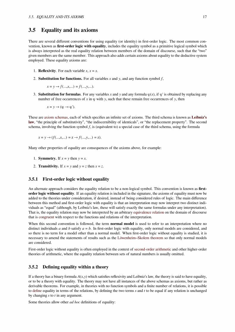
There are several different conventions for using equality (or identity) in first-order logic. The most common con-vention, known as first-order logic with equality, includes the equality symbol as a primitive logical symbol whichis always interpreted as the real equality relation between members of the domain of discourse, such that the “two”given members are the same member. This approach also adds certain axioms about equality to the deductive systememployed. These equality axioms are:

1. Reflexivity. For each variable x, x = x.

2. Substitution for functions. For all variables x and y, and any function symbol f,

x = y→ f(...,x,...) = f(...,y,...).

3. Substitution for formulas. For any variables x and y and any formula φ(x), if φ' is obtained by replacing anynumber of free occurrences of x in φ with y, such that these remain free occurrences of y, then

x = y→ (φ → φ').

These are axiom schemas, each of which specifies an infinite set of axioms. The third schema is known as Leibniz’slaw, “the principle of substitutivity”, “the indiscernibility of identicals”, or “the replacement property”. The secondschema, involving the function symbol f, is (equivalent to) a special case of the third schema, using the formula

x = y→ (f(...,x,...) = z → f(...,y,...) = z).

Many other properties of equality are consequences of the axioms above, for example:

1. Symmetry. If x = y then y = x.

2. Transitivity. If x = y and y = z then x = z.

3.5.1 First-order logic without equality

An alternate approach considers the equality relation to be a non-logical symbol. This convention is known as first-order logic without equality. If an equality relation is included in the signature, the axioms of equality must now beadded to the theories under consideration, if desired, instead of being considered rules of logic. The main differencebetween this method and first-order logic with equality is that an interpretation may now interpret two distinct indi-viduals as “equal” (although, by Leibniz’s law, these will satisfy exactly the same formulas under any interpretation).That is, the equality relation may now be interpreted by an arbitrary equivalence relation on the domain of discoursethat is congruent with respect to the functions and relations of the interpretation.When this second convention is followed, the term normal model is used to refer to an interpretation where nodistinct individuals a and b satisfy a = b. In first-order logic with equality, only normal models are considered, andso there is no term for a model other than a normal model. When first-order logic without equality is studied, it isnecessary to amend the statements of results such as the Löwenheim–Skolem theorem so that only normal modelsare considered.First-order logic without equality is often employed in the context of second-order arithmetic and other higher-ordertheories of arithmetic, where the equality relation between sets of natural numbers is usually omitted.

3.5.2 Defining equality within a theory

If a theory has a binary formula A(x,y) which satisfies reflexivity and Leibniz’s law, the theory is said to have equality,or to be a theory with equality. The theory may not have all instances of the above schemas as axioms, but rather asderivable theorems. For example, in theories with no function symbols and a finite number of relations, it is possibleto define equality in terms of the relations, by defining the two terms s and t to be equal if any relation is unchangedby changing s to t in any argument.Some theories allow other ad hoc definitions of equality:

18 CHAPTER 3. FIRST-ORDER LOGIC

• In the theory of partial orders with one relation symbol ≤, one could define s = t to be an abbreviation for s ≤ t∧ t ≤ s.

• In set theory with one relation ∈ , one may define s = t to be an abbreviation for ∀ x (s ∈ x ↔ t ∈ x) ∧ ∀x (x ∈ s ↔ x ∈ t). This definition of equality then automatically satisfies the axioms for equality. In thiscase, one should replace the usual axiom of extensionality, ∀x∀y[∀z(z ∈ x ⇔ z ∈ y) ⇒ x = y] , by∀x∀y[∀z(z ∈ x⇔ z ∈ y) ⇒ ∀z(x ∈ z ⇔ y ∈ z)] , i.e. if x and y have the same elements, then they belongto the same sets.

3.6 Metalogical properties

One motivation for the use of first-order logic, rather than higher-order logic, is that first-order logic has manymetalogical properties that stronger logics do not have. These results concern general properties of first-order logicitself, rather than properties of individual theories. They provide fundamental tools for the construction of modelsof first-order theories.

3.6.1 Completeness and undecidability

Gödel’s completeness theorem, proved by Kurt Gödel in 1929, establishes that there are sound, complete, effectivedeductive systems for first-order logic, and thus the first-order logical consequence relation is captured by finite prov-ability. Naively, the statement that a formula φ logically implies a formula ψ depends on every model of φ; thesemodels will in general be of arbitrarily large cardinality, and so logical consequence cannot be effectively verified bychecking every model. However, it is possible to enumerate all finite derivations and search for a derivation of ψ fromφ. If ψ is logically implied by φ, such a derivation will eventually be found. Thus first-order logical consequence issemidecidable: it is possible to make an effective enumeration of all pairs of sentences (φ,ψ) such that ψ is a logicalconsequence of φ.Unlike propositional logic, first-order logic is undecidable (although semidecidable), provided that the language hasat least one predicate of arity at least 2 (other than equality). This means that there is no decision procedure thatdetermines whether arbitrary formulas are logically valid. This result was established independently byAlonzo Churchand Alan Turing in 1936 and 1937, respectively, giving a negative answer to the Entscheidungsproblem posed byDavid Hilbert in 1928. Their proofs demonstrate a connection between the unsolvability of the decision problem forfirst-order logic and the unsolvability of the halting problem.There are systems weaker than full first-order logic for which the logical consequence relation is decidable. Theseinclude propositional logic andmonadic predicate logic, which is first-order logic restricted to unary predicate symbolsand no function symbols. Other logics with no function symbols which are decidable are the guarded fragment offirst-order logic, as well as two-variable logic. The Bernays–Schönfinkel class of first-order formulas is also decidable.Decidable subsets of first-order logic are also studied in the framework of description logics.

3.6.2 The Löwenheim–Skolem theorem

The Löwenheim–Skolem theorem shows that if a first-order theory of cardinality λ has an infinite model, then it hasmodels of every infinite cardinality greater than or equal to λ. One of the earliest results in model theory, it impliesthat it is not possible to characterize countability or uncountability in a first-order language. That is, there is nofirst-order formula φ(x) such that an arbitrary structure M satisfies φ if and only if the domain of discourse of M iscountable (or, in the second case, uncountable).The Löwenheim–Skolem theorem implies that infinite structures cannot be categorically axiomatized in first-orderlogic. For example, there is no first-order theory whose only model is the real line: any first-order theory with aninfinite model also has a model of cardinality larger than the continuum. Since the real line is infinite, any theorysatisfied by the real line is also satisfied by some nonstandard models. When the Löwenheim–Skolem theorem isapplied to first-order set theories, the nonintuitive consequences are known as Skolem’s paradox.

3.7. LIMITATIONS 19

3.6.3 The compactness theorem

The compactness theorem states that a set of first-order sentences has a model if and only if every finite subset of ithas a model. This implies that if a formula is a logical consequence of an infinite set of first-order axioms, then itis a logical consequence of some finite number of those axioms. This theorem was proved first by Kurt Gödel as aconsequence of the completeness theorem, but many additional proofs have been obtained over time. It is a centraltool in model theory, providing a fundamental method for constructing models.The compactness theorem has a limiting effect on which collections of first-order structures are elementary classes.For example, the compactness theorem implies that any theory that has arbitrarily large finite models has an infi-nite model. Thus the class of all finite graphs is not an elementary class (the same holds for many other algebraicstructures).There are also more subtle limitations of first-order logic that are implied by the compactness theorem. For example,in computer science, many situations can be modeled as a directed graph of states (nodes) and connections (directededges). Validating such a system may require showing that no “bad” state can be reached from any “good” state. Thusone seeks to determine if the good and bad states are in different connected components of the graph. However, thecompactness theorem can be used to show that connected graphs are not an elementary class in first-order logic,and there is no formula φ(x,y) of first-order logic, in the signature of graphs, that expresses the idea that there is apath from x to y. Connectedness can be expressed in second-order logic, however, but not with only existential setquantifiers, as Σ1

1 also enjoys compactness.

3.6.4 Lindström’s theorem

Main article: Lindström’s theorem

Per Lindström showed that the metalogical properties just discussed actually characterize first-order logic in the sensethat no stronger logic can also have those properties (Ebbinghaus and Flum 1994, Chapter XIII). Lindström defineda class of abstract logical systems, and a rigorous definition of the relative strength of a member of this class. Heestablished two theorems for systems of this type:

• A logical system satisfying Lindström’s definition that contains first-order logic and satisfies both the Löwenheim–Skolem theorem and the compactness theorem must be equivalent to first-order logic.

• A logical system satisfying Lindström’s definition that has a semidecidable logical consequence relation andsatisfies the Löwenheim–Skolem theorem must be equivalent to first-order logic.

3.7 Limitations

Although first-order logic is sufficient for formalizing much of mathematics, and is commonly used in computerscience and other fields, it has certain limitations. These include limitations on its expressiveness and limitations ofthe fragments of natural languages that it can describe.For instance, first-order logic is undecidable, meaning a sound, complete and terminating decision algorithm is im-possible. This has led to the study of interesting decidable fragments such as C2, first-order logic with two variablesand the counting quantifiers ∃≥n and ∃≤n (these quantifiers are, respectively, “there exists at least n" and “there existsat most n") (Horrocks 2010).

3.7.1 Expressiveness

The Löwenheim–Skolem theorem shows that if a first-order theory has any infinite model, then it has infinite modelsof every cardinality. In particular, no first-order theory with an infinite model can be categorical. Thus there isno first-order theory whose only model has the set of natural numbers as its domain, or whose only model has theset of real numbers as its domain. Many extensions of first-order logic, including infinitary logics and higher-orderlogics, are more expressive in the sense that they do permit categorical axiomatizations of the natural numbers orreal numbers. This expressiveness comes at a metalogical cost, however: by Lindström’s theorem, the compactnesstheorem and the downward Löwenheim–Skolem theorem cannot hold in any logic stronger than first-order.

20 CHAPTER 3. FIRST-ORDER LOGIC

3.7.2 Formalizing natural languages

First-order logic is able to formalize many simple quantifier constructions in natural language, such as “every personwho lives in Perth lives in Australia”. But there are many more complicated features of natural language that cannotbe expressed in (single-sorted) first-order logic. “Any logical system which is appropriate as an instrument for theanalysis of natural language needs a much richer structure than first-order predicate logic” (Gamut 1991, p. 75).

3.8 Restrictions, extensions, and variations

There are many variations of first-order logic. Some of these are inessential in the sense that they merely changenotation without affecting the semantics. Others change the expressive power more significantly, by extending thesemantics through additional quantifiers or other new logical symbols. For example, infinitary logics permit formulasof infinite size, and modal logics add symbols for possibility and necessity.

3.8.1 Restricted languages

First-order logic can be studied in languages with fewer logical symbols than were described above.

• Because ∃xϕ(x) can be expressed as ¬∀x¬ϕ(x) , and ∀xϕ(x) can be expressed as ¬∃x¬ϕ(x) , either of thetwo quantifiers ∃ and ∀ can be dropped.

• Since ϕ∨ψ can be expressed as ¬(¬ϕ∧¬ψ) and ϕ∧ψ can be expressed as ¬(¬ϕ∨¬ψ) , either ∨ or ∧ canbe dropped. In other words, it is sufficient to have ¬ and ∨ , or ¬ and ∧ , as the only logical connectives.

• Similarly, it is sufficient to have only¬ and→ as logical connectives, or to have only the Sheffer stroke (NAND)or the Peirce arrow (NOR) operator.

• It is possible to entirely avoid function symbols and constant symbols, rewriting them via predicate symbolsin an appropriate way. For example, instead of using a constant symbol 0 one may use a predicate 0(x)(interpreted as x = 0 ), and replace every predicate such as P (0, y) with ∀x (0(x) → P (x, y)) . Afunction such as f(x1, x2, ..., xn) will similarly be replaced by a predicate F (x1, x2, ..., xn, y) interpretedas y = f(x1, x2, ..., xn) . This change requires adding additional axioms to the theory at hand, so thatinterpretations of the predicate symbols used have the correct semantics.

Restrictions such as these are useful as a technique to reduce the number of inference rules or axiom schemas indeductive systems, which leads to shorter proofs of metalogical results. The cost of the restrictions is that it becomesmore difficult to express natural-language statements in the formal system at hand, because the logical connectivesused in the natural language statements must be replaced by their (longer) definitions in terms of the restricted col-lection of logical connectives. Similarly, derivations in the limited systems may be longer than derivations in systemsthat include additional connectives. There is thus a trade-off between the ease of working within the formal systemand the ease of proving results about the formal system.It is also possible to restrict the arities of function symbols and predicate symbols, in sufficiently expressive theories.One can in principle dispense entirely with functions of arity greater than 2 and predicates of arity greater than 1in theories that include a pairing function. This is a function of arity 2 that takes pairs of elements of the domainand returns an ordered pair containing them. It is also sufficient to have two predicate symbols of arity 2 that defineprojection functions from an ordered pair to its components. In either case it is necessary that the natural axioms fora pairing function and its projections are satisfied.

3.8.2 Many-sorted logic

Ordinary first-order interpretations have a single domain of discourse over which all quantifiers range. Many-sortedfirst-order logic allows variables to have different sorts, which have different domains. This is also called typed first-order logic, and the sorts called types (as in data type), but it is not the same as first-order type theory. Many-sortedfirst-order logic is often used in the study of second-order arithmetic.

3.8. RESTRICTIONS, EXTENSIONS, AND VARIATIONS 21

When there are only finitely many sorts in a theory, many-sorted first-order logic can be reduced to single-sorted first-order logic. One introduces into the single-sorted theory a unary predicate symbol for each sort in the many-sortedtheory, and adds an axiom saying that these unary predicates partition the domain of discourse. For example, if thereare two sorts, one adds predicate symbols P1(x) and P2(x) and the axiom

∀x(P1(x) ∨ P2(x)) ∧ ¬∃x(P1(x) ∧ P2(x))

Then the elements satisfying P1 are thought of as elements of the first sort, and elements satisfying P2 as elementsof the second sort. One can quantify over each sort by using the corresponding predicate symbol to limit the rangeof quantification. For example, to say there is an element of the first sort satisfying formula φ(x), one writes

∃x(P1(x) ∧ ϕ(x))

3.8.3 Additional quantifiers

Additional quantifiers can be added to first-order logic.

• Sometimes it is useful to say that "P(x) holds for exactly one x", which can be expressed as ∃! x P(x). Thisnotation, called uniqueness quantification, may be taken to abbreviate a formula such as ∃ x (P(x) ∧∀ y (P(y)→ (x = y))).

• First-order logic with extra quantifiers has new quantifiers Qx,..., with meanings such as “there are many xsuch that ...”. Also see branching quantifiers and the plural quantifiers of George Boolos and others.

• Bounded quantifiers are often used in the study of set theory or arithmetic.

3.8.4 Infinitary logics

Main article: Infinitary logic

Infinitary logic allows infinitely long sentences. For example, one may allow a conjunction or disjunction of infinitelymany formulas, or quantification over infinitely many variables. Infinitely long sentences arise in areas of mathematicsincluding topology and model theory.Infinitary logic generalizes first-order logic to allow formulas of infinite length. The most common way in whichformulas can become infinite is through infinite conjunctions and disjunctions. However, it is also possible to admitgeneralized signatures in which function and relation symbols are allowed to have infinite arities, or in which quantifierscan bind infinitely many variables. Because an infinite formula cannot be represented by a finite string, it is necessaryto choose some other representation of formulas; the usual representation in this context is a tree. Thus formulas are,essentially, identified with their parse trees, rather than with the strings being parsed.The most commonly studied infinitary logics are denoted Lαᵦ, where α and β are each either cardinal numbersor the symbol ∞. In this notation, ordinary first-order logic is Lωω. In the logic L∞ω, arbitrary conjunctions ordisjunctions are allowed when building formulas, and there is an unlimited supply of variables. More generally, thelogic that permits conjunctions or disjunctions with less than κ constituents is known as Lκω. For example, Lω1ωpermits countable conjunctions and disjunctions.The set of free variables in a formula of Lκω can have any cardinality strictly less than κ, yet only finitely many ofthem can be in the scope of any quantifier when a formula appears as a subformula of another.[8] In other infinitarylogics, a subformula may be in the scope of infinitely many quantifiers. For example, in Lκ∞, a single universal or ex-istential quantifier may bind arbitrarily many variables simultaneously. Similarly, the logic Lκλ permits simultaneousquantification over fewer than λ variables, as well as conjunctions and disjunctions of size less than κ.

3.8.5 Non-classical and modal logics

• Intuitionistic first-order logic uses intuitionistic rather than classical propositional calculus; for example, ¬¬φneed not be equivalent to φ.

22 CHAPTER 3. FIRST-ORDER LOGIC

• First-order modal logic allows one to describe other possible worlds as well as this contingently true worldwhich we inhabit. In some versions, the set of possible worlds varies depending on which possible world oneinhabits. Modal logic has extra modal operators with meanings which can be characterized informally as, forexample “it is necessary that φ" (true in all possible worlds) and “it is possible that φ" (true in some possibleworld). With standard first-order logic we have a single domain and each predicate is assigned one extension.With first-order modal logic we have a domain function that assigns each possible world its own domain, so thateach predicate gets an extension only relative to these possible worlds. This allows us to model cases where,for example, Alex is a Philosopher, but might have been a Mathematician, and might not have existed at all.In the first possible world P(a) is true, in the second P(a) is false, and in the third possible world there is no ain the domain at all.

• first-order fuzzy logics are first-order extensions of propositional fuzzy logics rather than classical propositionalcalculus.

3.8.6 Fixpoint logic

Fixpoint logic extends first-order logic by adding the closure under the least fixed points of positive operators.[9]

3.8.7 Higher-order logics

Main article: Higher-order logic

The characteristic feature of first-order logic is that individuals can be quantified, but not predicates. Thus

∃a(Phil(a))

is a legal first-order formula, but

∃Phil(Phil(a))

is not, in most formalizations of first-order logic. Second-order logic extends first-order logic by adding the lattertype of quantification. Other higher-order logics allow quantification over even higher types than second-order logicpermits. These higher types include relations between relations, functions from relations to relations between relations,and other higher-type objects. Thus the “first” in first-order logic describes the type of objects that can be quantified.Unlike first-order logic, for which only one semantics is studied, there are several possible semantics for second-order logic. The most commonly employed semantics for second-order and higher-order logic is known as fullsemantics. The combination of additional quantifiers and the full semantics for these quantifiers makes higher-orderlogic stronger than first-order logic. In particular, the (semantic) logical consequence relation for second-order andhigher-order logic is not semidecidable; there is no effective deduction system for second-order logic that is soundand complete under full semantics.Second-order logic with full semantics is more expressive than first-order logic. For example, it is possible to createaxiom systems in second-order logic that uniquely characterize the natural numbers and the real line. The cost ofthis expressiveness is that second-order and higher-order logics have fewer attractive metalogical properties than first-order logic. For example, the Löwenheim–Skolem theorem and compactness theorem of first-order logic becomefalse when generalized to higher-order logics with full semantics.

3.9 Automated theorem proving and formal methods

Further information: First-order theorem proving

Automated theorem proving refers to the development of computer programs that search and find derivations (formalproofs) of mathematical theorems. Finding derivations is a difficult task because the search space can be very large; an

3.10. SEE ALSO 23

exhaustive search of every possible derivation is theoretically possible but computationally infeasible for many systemsof interest in mathematics. Thus complicated heuristic functions are developed to attempt to find a derivation in lesstime than a blind search.The related area of automated proof verification uses computer programs to check that human-created proofs arecorrect. Unlike complicated automated theorem provers, verification systems may be small enough that their correct-ness can be checked both by hand and through automated software verification. This validation of the proof verifieris needed to give confidence that any derivation labeled as “correct” is actually correct.Some proof verifiers, such as Metamath, insist on having a complete derivation as input. Others, such as Mizar andIsabelle, take a well-formatted proof sketch (which may still be very long and detailed) and fill in the missing piecesby doing simple proof searches or applying known decision procedures: the resulting derivation is then verified by asmall, core “kernel”. Many such systems are primarily intended for interactive use by human mathematicians: theseare known as proof assistants. They may also use formal logics that are stronger than first-order logic, such as typetheory. Because a full derivation of any nontrivial result in a first-order deductive system will be extremely long fora human to write,[10] results are often formalized as a series of lemmas, for which derivations can be constructedseparately.Automated theorem provers are also used to implement formal verification in computer science. In this setting,theorem provers are used to verify the correctness of programs and of hardware such as processors with respect to aformal specification. Because such analysis is time-consuming and thus expensive, it is usually reserved for projectsin which a malfunction would have grave human or financial consequences.

3.10 See also• ACL2 — A Computational Logic for Applicative Common Lisp.

• Equiconsistency

• Extension by definitions

• Herbrandization

• Higher-order logic

• List of logic symbols

• Löwenheim number

• Prenex normal form

• Relational algebra

• Relational model

• Second-order logic

• Skolem normal form

• Tarski’s World

• Truth table

• Type (model theory)

3.11 Notes[1] Mendelson, Elliott (1964). Introduction to Mathematical Logic. Van Nostrand Reinhold. p. 56.

[2] The word language is sometimes used as a synonym for signature, but this can be confusing because “language” can alsorefer to the set of formulas.

[3] More precisely, there is only one language of each variant of one-sorted first-order logic: with or without equality, with orwithout functions, with or without propositional variables, ....

24 CHAPTER 3. FIRST-ORDER LOGIC

[4] Some authors who use the term “well-formed formula” use “formula” to mean any string of symbols from the alphabet.However, most authors in mathematical logic use “formula” to mean “well-formed formula” and have no term for non-well-formed formulas. In every context, it is only the well-formed formulas that are of interest.

[5] The SMT-LIB Standard: Version 2.0, by Clark Barrett, Aaron Stump, and Cesare Tinelli. http://smtlib.cs.uiowa.edu/language.shtml

[6] e.g. the matrix shown at 4

[7] e.g. the matrix shown at 2

[8] Some authors only admit formulas with finitely many free variables in Lκω, and more generally only formulas with < λ freevariables in Lκλ.

[9] Bosse, Uwe (1993). “An Ehrenfeucht–Fraïssé game for fixpoint logic and stratified fixpoint logic”. In Börger, Egon.Computer Science Logic: 6th Workshop, CSL'92, San Miniato, Italy, September 28 - October 2, 1992. Selected Papers.Lecture Notes in Computer Science 702. Springer-Verlag. pp. 100–114. ISBN 3-540-56992-8. Zbl 0808.03024.

[10] Avigad et al. (2007) discuss the process of formally verifying a proof of the prime number theorem. The formalized proofrequired approximately 30,000 lines of input to the Isabelle proof verifier.

3.12 References

• Andrews, Peter B. (2002); An Introduction to Mathematical Logic and Type Theory: To Truth Through Proof,2nd ed., Berlin: Kluwer Academic Publishers. Available from Springer.

• Avigad, Jeremy; Donnelly, Kevin; Gray, David; and Raff, Paul (2007); “A formally verified proof of the primenumber theorem”, ACM Transactions on Computational Logic, vol. 9 no. 1 doi:10.1145/1297658.1297660

• Barwise, Jon (1977); “An Introduction to First-Order Logic”, in Barwise, Jon, ed. (1982). Handbook ofMathematical Logic. Studies in Logic and the Foundations of Mathematics. Amsterdam, NL: North-Holland.ISBN 978-0-444-86388-1.

• Barwise, Jon; and Etchemendy, John (2000); Language Proof and Logic, Stanford, CA: CSLI Publications(Distributed by the University of Chicago Press)

• Bocheński, Józef Maria (2007); A Précis of Mathematical Logic, Dordrecht, NL: D. Reidel, translated fromthe French and German editions by Otto Bird

• Ferreirós, José (2001); The Road to Modern Logic — An Interpretation, Bulletin of Symbolic Logic, Volume7, Issue 4, 2001, pp. 441–484, DOI 10.2307/2687794, JStor

• Gamut, L. T. F. (1991); Logic, Language, and Meaning, Volume 2: Intensional Logic and Logical Grammar,Chicago, IL: University of Chicago Press, ISBN 0-226-28088-8

• Hilbert, David; and Ackermann, Wilhelm (1950); Principles of Mathematical Logic, Chelsea (English transla-tion of Grundzüge der theoretischen Logik, 1928 German first edition)

• Hodges, Wilfrid (2001); “Classical Logic I: First Order Logic”, in Goble, Lou (ed.); The Blackwell Guide toPhilosophical Logic, Blackwell

• Ebbinghaus, Heinz-Dieter; Flum, Jörg; and Thomas, Wolfgang (1994); Mathematical Logic, UndergraduateTexts in Mathematics, Berlin, DE/New York, NY: Springer-Verlag, Second Edition, ISBN 978-0-387-94258-2

• Rautenberg,Wolfgang (2010),AConcise Introduction toMathematical Logic (3rd ed.), NewYork, NY: SpringerScience+Business Media, doi:10.1007/978-1-4419-1221-3, ISBN 978-1-4419-1220-6

• Tarski, Alfred andGivant, Steven (1987); AFormalization of Set Theory without Variables. Vol.41 ofAmericanMathematical Society colloquium publications, Providence RI: American Mathematical Society, ISBN 978-0821810415.

3.13. EXTERNAL LINKS 25

3.13 External links• Hazewinkel, Michiel, ed. (2001), “Predicate calculus”, Encyclopedia of Mathematics, Springer, ISBN 978-1-55608-010-4

• Stanford Encyclopedia of Philosophy: Shapiro, Stewart; "Classical Logic". Covers syntax, model theory, andmetatheory for first-order logic in the natural deduction style.

• Magnus, P. D.; forall x: an introduction to formal logic. Covers formal semantics and proof theory for first-order logic.

• Metamath: an ongoing online project to reconstruct mathematics as a huge first-order theory, using first-orderlogic and the axiomatic set theory ZFC. Principia Mathematica modernized.

• Podnieks, Karl; Introduction to mathematical logic

• Cambridge Mathematics Tripos Notes (typeset by John Fremlin). These notes cover part of a past CambridgeMathematics Tripos course taught to undergraduates students (usually) within their third year. The course isentitled “Logic, Computation and Set Theory” and covers Ordinals and cardinals, Posets and Zorn’s Lemma,Propositional logic, Predicate logic, Set theory and Consistency issues related to ZFC and other set theories.

• Tree Proof Generator can validate or invalidate formulas of FOL through the semantic tableaux method.

26 CHAPTER 3. FIRST-ORDER LOGIC

A tableaux proof for the propositional formula ((a ∨ ~b) & b) → a.

Chapter 4

Propositional calculus

Propositional calculus (also called propositional logic, sentential calculus, or sentential logic) is the branch ofmathematical logic concerned with the study of propositions (whether they are true or false) that are formed by otherpropositions with the use of logical connectives, and how their value depends on the truth value of their components.Logical connectives are found in natural languages. In English for example, some examples are “and” (conjunction),“or” (disjunction), “not” (negation) and “if” (but only when used to denote material conditional).The following is an example of a very simple inference within the scope of propositional logic:

Premise 1: If it’s raining then it’s cloudy.Premise 2: It’s raining.Conclusion: It’s cloudy.

Both premises and the conclusions are propositions. The premises are taken for granted and then with the applicationof modus ponens (an inference rule) the conclusion follows.As propositional logic is not concerned with the structure of propositions beyond the point where they can't be decom-posed anymore by logical connectives, this inference can be restated replacing those atomic statements with statementletters, which are interpreted as variables representing statements:

P → Q

P

Q

The same can be stated succinctly in the following way:

P → Q,P ⊢ Q

When P is interpreted as “It’s raining” and Q as “it’s cloudy” the above symbolic expressions can be seen to exactlycorrespond with the original expression in natural language. Not only that, but they will also correspond with anyother inference of this form, which will be valid on the same basis that this inference is.Propositional logic may be studied through a formal system in which formulas of a formal languagemay be interpretedto represent propositions. A system of inference rules and axioms allows certain formulas to be derived. Thesederived formulas are called theorems and may be interpreted to be true propositions. A constructed sequence of suchformulas is known as a derivation or proof and the last formula of the sequence is the theorem. The derivation maybe interpreted as proof of the proposition represented by the theorem.When a formal system is used to represent formal logic, only statement letters are represented directly. The naturallanguage propositions that arise when they're interpreted are outside the scope of the system, and the relation betweenthe formal system and its interpretation is likewise outside the formal system itself.Usually in truth-functional propositional logic, formulas are interpreted as having either a truth value of true or atruth value of false. Truth-functional propositional logic and systems isomorphic to it, are considered to be zeroth-order logic.

27

28 CHAPTER 4. PROPOSITIONAL CALCULUS

4.1 History

Main article: History of logic

Although propositional logic (which is interchangeable with propositional calculus) had been hinted by earlier philoso-phers, it was developed into a formal logic by Chrysippus in the 3rd century BC[1] and expanded by the Stoics. Thelogic was focused on propositions. This advancement was different from the traditional syllogistic logic which was fo-cused on terms. However, later in antiquity, the propositional logic developed by the Stoics was no longer understood. Consequently, the system was essentially reinvented by Peter Abelard in the 12th century.[2]

Propositional logic was eventually refined using symbolic logic. The 17th/18th century philosopher Gottfried Leibnizhas been credited with being the founder of symbolic logic for his work with the calculus ratiocinator. Although hiswork was the first of its kind, it was unknown to the larger logical community. Consequently, many of the advancesachieved by Leibniz were reachieved by logicians likeGeorge Boole andAugustus DeMorgan completely independentof Leibniz.[3]

Just as propositional logic can be considered an advancement from the earlier syllogistic logic, Gottlob Frege’spredicate logic was an advancement from the earlier propositional logic. One author describes predicate logic ascombining “the distinctive features of syllogistic logic and propositional logic.”[4] Consequently, predicate logic ush-ered in a new era in logic’s history; however, advances in propositional logic were still made after Frege, includingNatural Deduction, Truth-Trees and Truth-Tables. Natural deduction was invented by Gerhard Gentzen and JanŁukasiewicz. Truth-Trees were invented by Evert Willem Beth.[5] The invention of truth-tables, however, is of con-troversial attribution.Within works by Frege[6] and BertrandRussell,[7] one finds ideas influential in bringing about the notion of truth tables.The actual 'tabular structure' (being formatted as a table), itself, is generally credited to either LudwigWittgenstein orEmil Post (or both, independently).[6] Besides Frege and Russell, others credited with having ideas preceding truth-tables include Philo, Boole, Charles Sanders Peirce, and Ernst Schröder. Others credited with the tabular structureinclude Łukasiewicz, Schröder, Alfred North Whitehead, William Stanley Jevons, John Venn, and Clarence IrvingLewis.[7] Ultimately, some have concluded, like John Shosky, that “It is far from clear that any one person should begiven the title of 'inventor' of truth-tables.”.[7]

4.2 Terminology

In general terms, a calculus is a formal system that consists of a set of syntactic expressions (well-formed formulas),a distinguished subset of these expressions (axioms), plus a set of formal rules that define a specific binary relation,intended to be interpreted to be logical equivalence, on the space of expressions.When the formal system is intended to be a logical system, the expressions aremeant to be interpreted to be statements,and the rules, known to be inference rules, are typically intended to be truth-preserving. In this setting, the rules (whichmay include axioms) can then be used to derive (“infer”) formulas representing true statements from given formulasrepresenting true statements.The set of axioms may be empty, a nonempty finite set, a countably infinite set, or be given by axiom schemata. Aformal grammar recursively defines the expressions and well-formed formulas of the language. In addition a semanticsmay be given which defines truth and valuations (or interpretations).The language of a propositional calculus consists of

1. a set of primitive symbols, variously referred to be atomic formulas, placeholders, proposition letters, or vari-ables, and

2. a set of operator symbols, variously interpreted to be logical operators or logical connectives.

A well-formed formula is any atomic formula, or any formula that can be built up from atomic formulas by means ofoperator symbols according to the rules of the grammar.Mathematicians sometimes distinguish between propositional constants, propositional variables, and schemata. Propo-sitional constants represent some particular proposition, while propositional variables range over the set of all atomicpropositions. Schemata, however, range over all propositions. It is common to represent propositional constants by

4.3. BASIC CONCEPTS 29

A, B, and C, propositional variables by P, Q, and R, and schematic letters are often Greek letters, most often φ, ψ,and χ.

4.3 Basic concepts

The following outlines a standard propositional calculus. Many different formulations exist which are all more or lessequivalent but differ in the details of:

1. their language, that is, the particular collection of primitive symbols and operator symbols,2. the set of axioms, or distinguished formulas, and3. the set of inference rules.

Any given proposition may be represented with a letter called a 'propositional constant', analogous to representing anumber by a letter in mathematics, for instance, a = 5. All propositions require exactly one of two truth-values: trueor false. For example, let P be the proposition that it is raining outside. This will be true (P) if it is raining outsideand false otherwise (¬P).

• We then define truth-functional operators, beginning with negation. (¬P represents the negation of P, whichcan be thought of as the denial of P. In the example above, (¬P expresses that it is not raining outside, or by amore standard reading: “It is not the case that it is raining outside.” When P is true, (¬P is false; and when Pis false, (¬P is true. (¬¬P always has the same truth-value as P.

• Conjunction is a truth-functional connective which forms a proposition out of two simpler propositions, forexample, P and Q. The conjunction of P and Q is written P ∧ Q, and expresses that each are true. We read P∧ Q for “P and Q”. For any two propositions, there are four possible assignments of truth values:1. P is true and Q is true2. P is true and Q is false3. P is false and Q is true4. P is false and Q is false

The conjunction of P and Q is true in case 1 and is false otherwise. Where P is the proposition that it israining outside and Q is the proposition that a cold-front is over Kansas, P ∧ Q is true when it is rainingoutside and there is a cold-front over Kansas. If it is not raining outside, then P ∧ Q is false; and if thereis no cold-front over Kansas, then P ∧ Q is false.

• Disjunction resembles conjunction in that it forms a proposition out of two simpler propositions. We write itP ∨ Q, and it is read “P or Q”. It expresses that either P or Q is true. Thus, in the cases listed above, thedisjunction of P and Q is true in all cases except 4. Using the example above, the disjunction expresses thatit is either raining outside or there is a cold front over Kansas. (Note, this use of disjunction is supposed toresemble the use of the English word “or”. However, it is most like the English inclusive “or”, which can beused to express the truth of at least one of two propositions. It is not like the English exclusive “or”, whichexpresses the truth of exactly one of two propositions. That is to say, the exclusive “or” is false when both Pand Q are true (case 1). An example of the exclusive or is: You may have a bagel or a pastry, but not both.Often in natural language, given the appropriate context, the addendum “but not both” is omitted but implied.In mathematics, however, “or” is always inclusive or; if exclusive or is meant it will be specified, possibly by“xor”.)

• Material conditional also joins two simpler propositions, and we write P → Q, which is read “if P then Q”.The proposition to the left of the arrow is called the antecedent and the proposition to the right is calledthe consequent. (There is no such designation for conjunction or disjunction, since they are commutativeoperations.) It expresses that Q is true whenever P is true. Thus it is true in every case above except case 2,because this is the only case when P is true but Q is not. Using the example, if P then Q expresses that if it israining outside then there is a cold-front over Kansas. The material conditional is often confused with physicalcausation. The material conditional, however, only relates two propositions by their truth-values—which is notthe relation of cause and effect. It is contentious in the literature whether the material implication representslogical causation.

30 CHAPTER 4. PROPOSITIONAL CALCULUS

• Biconditional joins two simpler propositions, and we write P ↔ Q, which is read “P if and only if Q”. Itexpresses that P and Q have the same truth-value, thus P if and only if Q is true in cases 1 and 4, and falseotherwise.

It is extremely helpful to look at the truth tables for these different operators, as well as themethod of analytic tableaux.

4.3.1 Closure under operations

Propositional logic is closed under truth-functional connectives. That is to say, for any proposition φ, ¬φ is also aproposition. Likewise, for any propositions φ and ψ, φ ∧ψ is a proposition, and similarly for disjunction, conditional,and biconditional. This implies that, for instance, φ ∧ ψ is a proposition, and so it can be conjoined with anotherproposition. In order to represent this, we need to use parentheses to indicate which proposition is conjoined withwhich. For instance, P ∧ Q ∧ R is not a well-formed formula, because we do not know if we are conjoining P ∧Q with R or if we are conjoining P with Q ∧ R. Thus we must write either (P ∧ Q) ∧ R to represent the former, orP ∧ (Q ∧ R) to represent the latter. By evaluating the truth conditions, we see that both expressions have the sametruth conditions (will be true in the same cases), and moreover that any proposition formed by arbitrary conjunctionswill have the same truth conditions, regardless of the location of the parentheses. This means that conjunction isassociative, however, one should not assume that parentheses never serve a purpose. For instance, the sentence P ∧(Q ∨ R) does not have the same truth conditions of (P ∧ Q) ∨ R, so they are different sentences distinguished only bythe parentheses. One can verify this by the truth-table method referenced above.Note: For any arbitrary number of propositional constants, we can form a finite number of cases which list theirpossible truth-values. A simple way to generate this is by truth-tables, in which one writes P, Q, ..., Z, for any list ofk propositional constants—that is to say, any list of propositional constants with k entries. Below this list, one writes2k rows, and below P one fills in the first half of the rows with true (or T) and the second half with false (or F). BelowQ one fills in one-quarter of the rows with T, then one-quarter with F, then one-quarter with T and the last quarterwith F. The next column alternates between true and false for each eighth of the rows, then sixteenths, and so on,until the last propositional constant varies between T and F for each row. This will give a complete listing of cases ortruth-value assignments possible for those propositional constants.

4.3.2 Argument

The propositional calculus then defines an argument to be a set of propositions. A valid argument is a set of proposi-tions, the last of which follows from—or is implied by—the rest. All other arguments are invalid. The simplest validargument is modus ponens, one instance of which is the following set of propositions:

1. P → Q2. P∴ Q

This is a set of three propositions, each line is a proposition, and the last follows from the rest. The first two lines arecalled premises, and the last line the conclusion. We say that any proposition C follows from any set of propositions(P1, ..., Pn) , if C must be true whenever every member of the set (P1, ..., Pn) is true. In the argument above, forany P and Q, whenever P → Q and P are true, necessarily Q is true. Notice that, when P is true, we cannot considercases 3 and 4 (from the truth table). When P → Q is true, we cannot consider case 2. This leaves only case 1, inwhich Q is also true. Thus Q is implied by the premises.This generalizes schematically. Thus, where φ and ψ may be any propositions at all,

1. φ→ ψ2. φ∴ ψ

Other argument forms are convenient, but not necessary. Given a complete set of axioms (see below for one suchset), modus ponens is sufficient to prove all other argument forms in propositional logic, thus they may be consideredto be a derivative. Note, this is not true of the extension of propositional logic to other logics like first-order logic.First-order logic requires at least one additional rule of inference in order to obtain completeness.

4.4. GENERIC DESCRIPTION OF A PROPOSITIONAL CALCULUS 31

The significance of argument in formal logic is that one may obtain new truths from established truths. In the firstexample above, given the two premises, the truth of Q is not yet known or stated. After the argument is made, Q isdeduced. In this way, we define a deduction system to be a set of all propositions that may be deduced from anotherset of propositions. For instance, given the set of propositions A = P ∨ Q,¬Q ∧ R, (P ∨ Q) → R , we candefine a deduction system, Γ, which is the set of all propositions which follow from A. Reiteration is always assumed,so P ∨Q,¬Q ∧ R, (P ∨Q) → R ∈ Γ . Also, from the first element of A, last element, as well as modus ponens,R is a consequence, and so R ∈ Γ . Because we have not included sufficiently complete axioms, though, nothingelse may be deduced. Thus, even though most deduction systems studied in propositional logic are able to deduce(P ∨Q) ↔ (¬P → Q) , this one is too weak to prove such a proposition.

4.4 Generic description of a propositional calculus

A propositional calculus is a formal system L = L (A, Ω, Z, I) , where:

• The alpha set A is a finite set of elements called proposition symbols or propositional variables. Syntacticallyspeaking, these are the most basic elements of the formal languageL , otherwise referred to as atomic formulasor terminal elements. In the examples to follow, the elements of A are typically the letters p, q, r, and so on.

• The omega set Ω is a finite set of elements called operator symbols or logical connectives. The set Ω is partitionedinto disjoint subsets as follows:

Ω = Ω0 ∪ Ω1 ∪ . . . ∪ Ωj ∪ . . . ∪ Ωm.

In this partition, Ωj is the set of operator symbols of arity j.

In the more familiar propositional calculi, Ω is typically partitioned as follows:

Ω1 = ¬,

Ω2 ⊆ ∧,∨,→,↔.

A frequently adopted convention treats the constant logical values as operators of arity zero, thus:

Ω0 = 0, 1.

Some writers use the tilde (~), or N, instead of ¬; and some use the ampersand (&), the prefixed K, or· instead of ∧ . Notation varies even more for the set of logical values, with symbols like false, true,F, T, or ⊥,⊤ all being seen in various contexts instead of 0, 1.

• The zeta set Z is a finite set of transformation rules that are called inference rules when they acquire logicalapplications.

• The iota set I is a finite set of initial points that are called axioms when they receive logical interpretations.

The language of L , also known as its set of formulas, well-formed formulas, is inductively defined by the followingrules:

32 CHAPTER 4. PROPOSITIONAL CALCULUS

1. Base: Any element of the alpha set A is a formula of L .

2. If p1, p2, . . . , pj are formulas and f is in Ωj , then (f(p1, p2, . . . , pj)) is a formula.

3. Closed: Nothing else is a formula of L .

Repeated applications of these rules permits the construction of complex formulas. For example:

1. By rule 1, p is a formula.

2. By rule 2, ¬p is a formula.

3. By rule 1, q is a formula.

4. By rule 2, (¬p ∨ q) is a formula.

4.5 Example 1. Simple axiom system

Let L1 = L(A,Ω,Z, I) , where A , Ω , Z , I are defined as follows:

• The alpha set A , is a finite set of symbols that is large enough to supply the needs of a given discussion, forexample:

A = p, q, r, s, t, u.

• Of the three connectives for conjunction, disjunction, and implication ( ∧,∨ , and →), one can be taken asprimitive and the other two can be defined in terms of it and negation (¬).[8] Indeed, all of the logical connectivescan be defined in terms of a sole sufficient operator. The biconditional (↔) can of course be defined in termsof conjunction and implication, with a↔ b defined as (a→ b) ∧ (b→ a) .

Ω = Ω1 ∪ Ω2

Ω1 = ¬,

Ω2 = →.

• An axiom system discovered by Jan Łukasiewicz formulates a propositional calculus in this language as follows.The axioms are all substitution instances of:

• (p→ (q → p))

• ((p→ (q → r)) → ((p→ q) → (p→ r)))

• ((¬p→ ¬q) → (q → p))

• The rule of inference is modus ponens (i.e., from p and (p→ q) , infer q). Then a ∨ b is defined as ¬a→ b ,and a ∧ b is defined as ¬(a→ ¬b) . This system is used in Metamath set.mm formal proof database.

4.6. EXAMPLE 2. NATURAL DEDUCTION SYSTEM 33

4.6 Example 2. Natural deduction system

Let L2 = L(A,Ω,Z, I) , where A , Ω , Z , I are defined as follows:

• The alpha set A , is a finite set of symbols that is large enough to supply the needs of a given discussion, forexample:

A = p, q, r, s, t, u.

• The omega set Ω = Ω1 ∪ Ω2 partitions as follows:

Ω1 = ¬,

Ω2 = ∧,∨,→,↔.

In the following example of a propositional calculus, the transformation rules are intended to be interpreted as theinference rules of a so-called natural deduction system. The particular system presented here has no initial points,which means that its interpretation for logical applications derives its theorems from an empty axiom set.

• The set of initial points is empty, that is, I = ∅ .

• The set of transformation rules, Z , is described as follows:

Our propositional calculus has ten inference rules. These rules allow us to derive other true formulas given a set offormulas that are assumed to be true. The first nine simply state that we can infer certain well-formed formulas fromother well-formed formulas. The last rule however uses hypothetical reasoning in the sense that in the premise of therule we temporarily assume an (unproven) hypothesis to be part of the set of inferred formulas to see if we can infera certain other formula. Since the first nine rules don't do this they are usually described as non-hypothetical rules,and the last one as a hypothetical rule.In describing the transformation rules, we may introduce a metalanguage symbol ⊢ . It is basically a convenientshorthand for saying “infer that”. The format is Γ ⊢ ψ , in which Γ is a (possibly empty) set of formulas calledpremises, and ψ is a formula called conclusion. The transformation rule Γ ⊢ ψ means that if every proposition in Γ isa theorem (or has the same truth value as the axioms), then ψ is also a theorem. Note that considering the followingrule Conjunction introduction, we will know whenever Γ has more than one formula, we can always safely reduce itinto one formula using conjunction. So for short, from that time on we may represent Γ as one formula instead of aset. Another omission for convenience is when Γ is an empty set, in which case Γ may not appear.

Negation introduction From (p→ q) and (p→ ¬q) , infer ¬p .

That is, (p→ q), (p→ ¬q) ⊢ ¬p .

Negation elimination From ¬p , infer (p→ r) .

That is, ¬p ⊢ (p→ r) .

Double negative elimination From ¬¬p , infer p.

That is, ¬¬p ⊢ p .

Conjunction introduction From p and q, infer (p ∧ q) .

That is, p, q ⊢ (p ∧ q) .

Conjunction elimination From (p ∧ q) , infer p.

From (p ∧ q) , infer q.

That is, (p ∧ q) ⊢ p and (p ∧ q) ⊢ q .

Disjunction introduction From p, infer (p ∨ q) .

From q, infer (p ∨ q) .

34 CHAPTER 4. PROPOSITIONAL CALCULUS

That is, p ⊢ (p ∨ q) and q ⊢ (p ∨ q) .

Disjunction elimination From (p ∨ q) and (p→ r) and (q → r) , infer r.

That is, p ∨ q, p→ r, q → r ⊢ r .

Biconditional introduction From (p→ q) and (q → p) , infer (p↔ q) .

That is, p→ q, q → p ⊢ (p↔ q) .

Biconditional elimination From (p↔ q) , infer (p→ q) .

From (p↔ q) , infer (q → p) .

That is, (p↔ q) ⊢ (p→ q) and (p↔ q) ⊢ (q → p) .

Modus ponens (conditional elimination) From p and (p→ q) , infer q.

That is, p, p→ q ⊢ q .

Conditional proof (conditional introduction) From [accepting p allows a proof of q], infer (p→ q) .

That is, (p ⊢ q) ⊢ (p→ q) .

4.7 Basic and derived argument forms

4.8 Proofs in propositional calculus

One of the main uses of a propositional calculus, when interpreted for logical applications, is to determine relationsof logical equivalence between propositional formulas. These relationships are determined by means of the availabletransformation rules, sequences of which are called derivations or proofs.In the discussion to follow, a proof is presented as a sequence of numbered lines, with each line consisting of a singleformula followed by a reason or justification for introducing that formula. Each premise of the argument, that is, anassumption introduced as an hypothesis of the argument, is listed at the beginning of the sequence and is marked asa “premise” in lieu of other justification. The conclusion is listed on the last line. A proof is complete if every linefollows from the previous ones by the correct application of a transformation rule. (For a contrasting approach, seeproof-trees).

4.8.1 Example of a proof

• To be shown that A→ A.

• One possible proof of this (which, though valid, happens to contain more steps than are necessary) may bearranged as follows:

Interpret A ⊢ A as “Assuming A, infer A”. Read ⊢ A→ A as “Assuming nothing, infer that A implies A”, or “It isa tautology that A implies A”, or “It is always true that A implies A”.

4.9 Soundness and completeness of the rules

The crucial properties of this set of rules are that they are sound and complete. Informally this means that the rulesare correct and that no other rules are required. These claims can be made more formal as follows.We define a truth assignment as a function that maps propositional variables to true or false. Informally such atruth assignment can be understood as the description of a possible state of affairs (or possible world) where certainstatements are true and others are not. The semantics of formulas can then be formalized by defining for which “stateof affairs” they are considered to be true, which is what is done by the following definition.We define when such a truth assignment A satisfies a certain well-formed formula with the following rules:

4.9. SOUNDNESS AND COMPLETENESS OF THE RULES 35

• A satisfies the propositional variable P if and only if A(P) = true

• A satisfies ¬φ if and only if A does not satisfy φ

• A satisfies (φ ∧ ψ) if and only if A satisfies both φ and ψ

• A satisfies (φ ∨ ψ) if and only if A satisfies at least one of either φ or ψ

• A satisfies (φ→ ψ) if and only if it is not the case that A satisfies φ but not ψ

• A satisfies (φ↔ ψ) if and only if A satisfies both φ and ψ or satisfies neither one of them

With this definition we can now formalize what it means for a formula φ to be implied by a certain set S of formulas.Informally this is true if in all worlds that are possible given the set of formulas S the formula φ also holds. Thisleads to the following formal definition: We say that a set S of well-formed formulas semantically entails (or implies)a certain well-formed formula φ if all truth assignments that satisfy all the formulas in S also satisfy φ.Finally we define syntactical entailment such that φ is syntactically entailed by S if and only if we can derive it withthe inference rules that were presented above in a finite number of steps. This allows us to formulate exactly what itmeans for the set of inference rules to be sound and complete:Soundness: If the set of well-formed formulas S syntactically entails the well-formed formula φ then S semanticallyentails φ.Completeness: If the set of well-formed formulas S semantically entails the well-formed formula φ then S syntac-tically entails φ.For the above set of rules this is indeed the case.

4.9.1 Sketch of a soundness proof

(For most logical systems, this is the comparatively “simple” direction of proof)Notational conventions: Let G be a variable ranging over sets of sentences. Let A, B and C range over sentences. For“G syntactically entails A” we write “G proves A”. For “G semantically entails A” we write “G implies A”.We want to show: (A)(G) (if G proves A, then G implies A).We note that “G proves A” has an inductive definition, and that gives us the immediate resources for demonstratingclaims of the form “If G proves A, then ...”. So our proof proceeds by induction.

1. Basis. Show: If A is a member of G, then G implies A.

2. Basis. Show: If A is an axiom, then G implies A.

3. Inductive step (induction on n, the length of the proof):

(a) Assume for arbitrary G and A that if G proves A in n or fewer steps, then G implies A.(b) For each possible application of a rule of inference at step n + 1, leading to a new theorem B, show that

G implies B.

Notice that Basis Step II can be omitted for natural deduction systems because they have no axioms. When used,Step II involves showing that each of the axioms is a (semantic) logical truth.The Basis steps demonstrate that the simplest provable sentences from G are also implied by G, for any G. (Theproof is simple, since the semantic fact that a set implies any of its members, is also trivial.) The Inductive step willsystematically cover all the further sentences that might be provable—by considering each case where we might reacha logical conclusion using an inference rule—and shows that if a new sentence is provable, it is also logically implied.(For example, we might have a rule telling us that from “A” we can derive “A or B”. In III.a We assume that if A isprovable it is implied. We also know that if A is provable then “A or B” is provable. We have to show that then “Aor B” too is implied. We do so by appeal to the semantic definition and the assumption we just made. A is provablefrom G, we assume. So it is also implied by G. So any semantic valuation making all of G true makes A true. Butany valuation making A true makes “A or B” true, by the defined semantics for “or”. So any valuation which makes

36 CHAPTER 4. PROPOSITIONAL CALCULUS

all of G true makes “A or B” true. So “A or B” is implied.) Generally, the Inductive step will consist of a lengthy butsimple case-by-case analysis of all the rules of inference, showing that each “preserves” semantic implication.By the definition of provability, there are no sentences provable other than by being a member of G, an axiom, orfollowing by a rule; so if all of those are semantically implied, the deduction calculus is sound.

4.9.2 Sketch of completeness proof

(This is usually the much harder direction of proof.)We adopt the same notational conventions as above.We want to show: If G implies A, then G proves A. We proceed by contraposition: We show instead that if G doesnot prove A then G does not imply A.

1. G does not prove A. (Assumption)

2. If G does not prove A, then we can construct an (infinite) Maximal Set, G∗, which is a superset of G andwhich also does not prove A.

(a) Place an ordering on all the sentences in the language (e.g., shortest first, and equally long ones in extendedalphabetical ordering), and number them (E1, E2, ...)

(b) Define a series G of sets (G0, G1, ...) inductively:

i. G0 = G

ii. If Gk ∪ Ek+1 proves A, then Gk+1 = Gk

iii. If Gk ∪ Ek+1 does not prove A, then Gk+1 = Gk ∪ Ek+1(c) Define G∗ as the union of all the G . (That is, G∗ is the set of all the sentences that are in any G .)(d) It can be easily shown that

i. G∗ contains (is a superset of) G (by (b.i));ii. G∗ does not prove A (because if it proves A then some sentence was added to some G which caused

it to prove A; but this was ruled out by definition); andiii. G∗ is a Maximal Set with respect to A: If any more sentences whatever were added to G∗, it would

prove A. (Because if it were possible to add any more sentences, they should have been added whenthey were encountered during the construction of the G , again by definition)

3. If G∗ is a Maximal Set with respect to A, then it is truth-like. This means that it contains C only if it does notcontain ¬C; If it contains C and contains “If C then B” then it also contains B; and so forth.

4. If G∗ is truth-like there is a G∗-Canonical valuation of the language: one that makes every sentence in G∗ trueand everything outside G∗ false while still obeying the laws of semantic composition in the language.

5. A G∗-canonical valuation will make our original set G all true, and make A false.

6. If there is a valuation on which G are true and A is false, then G does not (semantically) imply A.

QED

4.9.3 Another outline for a completeness proof

If a formula is a tautology, then there is a truth table for it which shows that each valuation yields the value true for theformula. Consider such a valuation. By mathematical induction on the length of the subformulas, show that the truthor falsity of the subformula follows from the truth or falsity (as appropriate for the valuation) of each propositionalvariable in the subformula. Then combine the lines of the truth table together two at a time by using "(P is true impliesS) implies ((P is false implies S) implies S)". Keep repeating this until all dependencies on propositional variableshave been eliminated. The result is that we have proved the given tautology. Since every tautology is provable, thelogic is complete.

4.10. INTERPRETATION OF A TRUTH-FUNCTIONAL PROPOSITIONAL CALCULUS 37

4.10 Interpretation of a truth-functional propositional calculus

An interpretation of a truth-functional propositional calculusP is an assignment to each propositional symbol ofP of one or the other (but not both) of the truth values truth (T) and falsity (F), and an assignment to the connectivesymbols of P of their usual truth-functional meanings. An interpretation of a truth-functional propositional calculusmay also be expressed in terms of truth tables.[10]

For n distinct propositional symbols there are 2n distinct possible interpretations. For any particular symbol a , forexample, there are 21 = 2 possible interpretations:

1. a is assigned T, or

2. a is assigned F.

For the pair a , b there are 22 = 4 possible interpretations:

1. both are assigned T,

2. both are assigned F,

3. a is assigned T and b is assigned F, or

4. a is assigned F and b is assigned T.[10]

Since P has ℵ0 , that is, denumerably many propositional symbols, there are 2ℵ0 = c , and therefore uncountablymany distinct possible interpretations of P .[10]

4.10.1 Interpretation of a sentence of truth-functional propositional logic

Main article: Interpretation (logic)

If φ and ψ are formulas of P and I is an interpretation of P then:

• A sentence of propositional logic is true under an interpretation I iff I assigns the truth valueT to that sentence.If a sentence is true under an interpretation, then that interpretation is called a model of that sentence.

• φ is false under an interpretation I iff φ is not true under I .[10]

• A sentence of propositional logic is logically valid if it is true under every interpretation

|= ϕ means that φ is logically valid

• A sentence ψ of propositional logic is a semantic consequence of a sentence φ iff there is no interpretationunder which φ is true and ψ is false.

• A sentence of propositional logic is consistent iff it is true under at least one interpretation. It is inconsistent ifit is not consistent.

Some consequences of these definitions:

• For any given interpretation a given formula is either true or false.[10]

• No formula is both true and false under the same interpretation.[10]

• φ is false for a given interpretation iff ¬ϕ is true for that interpretation; and φ is true under an interpretationiff ¬ϕ is false under that interpretation.[10]

• If φ and (ϕ→ ψ) are both true under a given interpretation, then ψ is true under that interpretation.[10]

• If |=P ϕ and |=P (ϕ→ ψ) , then |=P ψ .[10]

38 CHAPTER 4. PROPOSITIONAL CALCULUS

• ¬ϕ is true under I iff φ is not true under I .

• (ϕ→ ψ) is true under I iff either φ is not true under I or ψ is true under I .[10]

• A sentence ψ of propositional logic is a semantic consequence of a sentence φ iff (ϕ → ψ) is logically valid,that is, ϕ |=P ψ iff |=P (ϕ→ ψ) .[10]

4.11 Alternative calculus

It is possible to define another version of propositional calculus, which defines most of the syntax of the logicaloperators by means of axioms, and which uses only one inference rule.

4.11.1 Axioms

Let φ, χ, and ψ stand for well-formed formulas. (The well-formed formulas themselves would not contain any Greekletters, but only capital Roman letters, connective operators, and parentheses.) Then the axioms are as follows:

• Axiom THEN-2 may be considered to be a “distributive property of implication with respect to implication.”

• Axioms AND-1 and AND-2 correspond to “conjunction elimination”. The relation between AND-1 and AND-2 reflects the commutativity of the conjunction operator.

• Axiom AND-3 corresponds to “conjunction introduction.”

• Axioms OR-1 and OR-2 correspond to “disjunction introduction.” The relation between OR-1 and OR-2 re-flects the commutativity of the disjunction operator.

• Axiom NOT-1 corresponds to “reductio ad absurdum.”

• Axiom NOT-2 says that “anything can be deduced from a contradiction.”

• Axiom NOT-3 is called "tertium non datur" (Latin: “a third is not given”) and reflects the semantic valuationof propositional formulas: a formula can have a truth-value of either true or false. There is no third truth-value,at least not in classical logic. Intuitionistic logicians do not accept the axiom NOT-3.

4.11.2 Inference rule

The inference rule is modus ponens:

ϕ, ϕ→ χ ⊢ χ

4.11.3 Meta-inference rule

Let a demonstration be represented by a sequence, with hypotheses to the left of the turnstile and the conclusion tothe right of the turnstile. Then the deduction theorem can be stated as follows:

If the sequence

ϕ1, ϕ2, ..., ϕn, χ ⊢ ψ

has been demonstrated, then it is also possible to demonstrate the sequence

ϕ1, ϕ2, ..., ϕn ⊢ χ→ ψ

4.11. ALTERNATIVE CALCULUS 39

This deduction theorem (DT) is not itself formulated with propositional calculus: it is not a theorem of propositionalcalculus, but a theorem about propositional calculus. In this sense, it is a meta-theorem, comparable to theoremsabout the soundness or completeness of propositional calculus.On the other hand, DT is so useful for simplifying the syntactical proof process that it can be considered and used asanother inference rule, accompanying modus ponens. In this sense, DT corresponds to the natural conditional proofinference rule which is part of the first version of propositional calculus introduced in this article.The converse of DT is also valid:

If the sequence

ϕ1, ϕ2, ..., ϕn ⊢ χ→ ψ

has been demonstrated, then it is also possible to demonstrate the sequence

ϕ1, ϕ2, ..., ϕn, χ ⊢ ψ

in fact, the validity of the converse of DT is almost trivial compared to that of DT:

If

ϕ1, ..., ϕn ⊢ χ→ ψ

then

ϕ1, ..., ϕn, χ ⊢ χ→ ψ

ϕ1, ..., ϕn, χ ⊢ χ

and from (1) and (2) can be deduced

ϕ1, ..., ϕn, χ ⊢ ψ

by means of modus ponens, Q.E.D.

The converse of DT has powerful implications: it can be used to convert an axiom into an inference rule. For example,the axiom AND-1,

⊢ ϕ ∧ χ→ ϕ

can be transformed by means of the converse of the deduction theorem into the inference rule

ϕ ∧ χ ⊢ ϕ

which is conjunction elimination, one of the ten inference rules used in the first version (in this article) of the propo-sitional calculus.

4.11.4 Example of a proof

The following is an example of a (syntactical) demonstration, involving only axioms THEN-1 and THEN-2:Prove: A→ A (Reflexivity of implication).Proof:

1. (A→ ((B → A) → A)) → ((A→ (B → A)) → (A→ A))

ϕ = A,χ = B → A,ψ = A

40 CHAPTER 4. PROPOSITIONAL CALCULUS

2. A→ ((B → A) → A)

ϕ = A,χ = B → A

3. (A→ (B → A)) → (A→ A)

From (1) and (2) by modus ponens.

4. A→ (B → A)

ϕ = A,χ = B

5. A→ A

From (3) and (4) by modus ponens.

4.12 Equivalence to equational logics

The preceding alternative calculus is an example of a Hilbert-style deduction system. In the case of propositionalsystems the axioms are terms built with logical connectives and the only inference rule is modus ponens. Equationallogic as standardly used informally in high school algebra is a different kind of calculus from Hilbert systems. Itstheorems are equations and its inference rules express the properties of equality, namely that it is a congruence onterms that admits substitution.Classical propositional calculus as described above is equivalent to Boolean algebra, while intuitionistic propositionalcalculus is equivalent to Heyting algebra. The equivalence is shown by translation in each direction of the theoremsof the respective systems. Theorems ϕ of classical or intuitionistic propositional calculus are translated as equationsϕ = 1 of Boolean or Heyting algebra respectively. Conversely theorems x = y of Boolean or Heyting algebra aretranslated as theorems (x → y) ∧ (y → x) of classical or intuitionistic calculus respectively, for which x ≡ y is astandard abbreviation. In the case of Boolean algebra x = y can also be translated as (x ∧ y) ∨ (¬x ∧ ¬y) , but thistranslation is incorrect intuitionistically.In both Boolean and Heyting algebra, inequality x ≤ y can be used in place of equality. The equality x = y isexpressible as a pair of inequalities x ≤ y and y ≤ x . Conversely the inequality x ≤ y is expressible as the equalityx ∧ y = x , or as x ∨ y = y . The significance of inequality for Hilbert-style systems is that it corresponds to thelatter’s deduction or entailment symbol ⊢ . An entailment

ϕ1, ϕ2, . . . , ϕn ⊢ ψ

is translated in the inequality version of the algebraic framework as

ϕ1 ∧ ϕ2 ∧ . . . ∧ ϕn ≤ ψ

Conversely the algebraic inequality x ≤ y is translated as the entailment

x ⊢ y

The difference between implication x→ y and inequality or entailment x ≤ y or x ⊢ y is that the former is internalto the logic while the latter is external. Internal implication between two terms is another term of the same kind.Entailment as external implication between two terms expresses a metatruth outside the language of the logic, andis considered part of the metalanguage. Even when the logic under study is intuitionistic, entailment is ordinarilyunderstood classically as two-valued: either the left side entails, or is less-or-equal to, the right side, or it is not.

4.13. GRAPHICAL CALCULI 41

Similar but more complex translations to and from algebraic logics are possible for natural deduction systems asdescribed above and for the sequent calculus. The entailments of the latter can be interpreted as two-valued, but amore insightful interpretation is as a set, the elements of which can be understood as abstract proofs organized asthe morphisms of a category. In this interpretation the cut rule of the sequent calculus corresponds to compositionin the category. Boolean and Heyting algebras enter this picture as special categories having at most one morphismper homset, i.e., one proof per entailment, corresponding to the idea that existence of proofs is all that matters: anyproof will do and there is no point in distinguishing them.

4.13 Graphical calculi

It is possible to generalize the definition of a formal language from a set of finite sequences over a finite basis to includemany other sets of mathematical structures, so long as they are built up by finitary means from finite materials. What’smore, many of these families of formal structures are especially well-suited for use in logic.For example, there are many families of graphs that are close enough analogues of formal languages that the conceptof a calculus is quite easily and naturally extended to them. Indeed, many species of graphs arise as parse graphsin the syntactic analysis of the corresponding families of text structures. The exigencies of practical computation onformal languages frequently demand that text strings be converted into pointer structure renditions of parse graphs,simply as a matter of checking whether strings are well-formed formulas or not. Once this is done, there are manyadvantages to be gained from developing the graphical analogue of the calculus on strings. The mapping from stringsto parse graphs is called parsing and the inverse mapping from parse graphs to strings is achieved by an operationthat is called traversing the graph.

4.14 Other logical calculi

Propositional calculus is about the simplest kind of logical calculus in current use. It can be extended in several ways.(Aristotelian “syllogistic” calculus, which is largely supplanted in modern logic, is in some ways simpler – but in otherways more complex – than propositional calculus.) The most immediate way to develop a more complex logicalcalculus is to introduce rules that are sensitive to more fine-grained details of the sentences being used.First-order logic (a.k.a. first-order predicate logic) results when the “atomic sentences” of propositional logic arebroken up into terms, variables, predicates, and quantifiers, all keeping the rules of propositional logic with somenew ones introduced. (For example, from “All dogs are mammals” we may infer “If Rover is a dog then Rover isa mammal”.) With the tools of first-order logic it is possible to formulate a number of theories, either with explicitaxioms or by rules of inference, that can themselves be treated as logical calculi. Arithmetic is the best known of these;others include set theory and mereology. Second-order logic and other higher-order logics are formal extensions offirst-order logic. Thus, it makes sense to refer to propositional logic as “zeroth-order logic”, when comparing it withthese logics.Modal logic also offers a variety of inferences that cannot be captured in propositional calculus. For example, from“Necessarily p” we may infer that p. From p we may infer “It is possible that p”. The translation between modallogics and algebraic logics concerns classical and intuitionistic logics but with the introduction of a unary operator onBoolean or Heyting algebras, different from the Boolean operations, interpreting the possibility modality, and in thecase of Heyting algebra a second operator interpreting necessity (for Boolean algebra this is redundant since necessityis the De Morgan dual of possibility). The first operator preserves 0 and disjunction while the second preserves 1 andconjunction.Many-valued logics are those allowing sentences to have values other than true and false. (For example, neither andboth are standard “extra values"; “continuum logic” allows each sentence to have any of an infinite number of “degreesof truth” between true and false.) These logics often require calculational devices quite distinct from propositionalcalculus. When the values form a Boolean algebra (which may have more than two or even infinitely many values),many-valued logic reduces to classical logic; many-valued logics are therefore only of independent interest when thevalues form an algebra that is not Boolean.

42 CHAPTER 4. PROPOSITIONAL CALCULUS

4.15 Solvers

Finding solutions to propositional logic formulas is an NP-complete problem. However, practical methods exist (e.g.,DPLL algorithm, 1962; Chaff algorithm, 2001) that are very fast for many useful cases. Recent work has extendedthe SAT solver algorithms to work with propositions containing arithmetic expressions; these are the SMT solvers.

4.16 See also

4.16.1 Higher logical levels• First-order logic• Second-order propositional logic• Second-order logic• Higher-order logic

4.16.2 Related topics

4.17 References[1] Ancient Logic (Stanford Encyclopedia of Philosophy)

[2] Marenbon, John (2007). Medieval philosophy: an historical and philosophical introduction. Routledge. p. 137.

[3] Leibniz’s Influence on 19th Century Logic

[4] Hurley, Patrick (2007). A Concise Introduction to Logic 10th edition. Wadsworth Publishing. p. 392.

[5] Beth, Evert W.; “Semantic entailment and formal derivability”, series: Mededlingen van de Koninklijke NederlandseAkademie van Wetenschappen, Afdeling Letterkunde, Nieuwe Reeks, vol. 18, no. 13, Noord-Hollandsche Uitg. Mij.,Amsterdam, 1955, pp. 309–42. Reprinted in Jaakko Intikka (ed.) The Philosophy of Mathematics, Oxford UniversityPress, 1969

[6] Truth in Frege

[7] Russell’s Use of Truth-Tables

[8] Wernick, William (1942) “Complete Sets of Logical Functions,” Transactions of the American Mathematical Society 51,pp. 117–132.

[9] Toida, Shunichi (2 August 2009). “Proof of Implications”. CS381 Discrete Structures/Discrete Mathematics Web CourseMaterial. Department Of Computer Science, Old Dominion University. Retrieved 10 March 2010.

[10] Hunter, Geoffrey (1971). Metalogic: An Introduction to the Metatheory of Standard First-Order Logic. University ofCalifornia Pres. ISBN 0-520-02356-0.

4.18 Further reading• Brown, Frank Markham (2003), Boolean Reasoning: The Logic of Boolean Equations, 1st edition, KluwerAcademic Publishers, Norwell, MA. 2nd edition, Dover Publications, Mineola, NY.

• Chang, C.C. and Keisler, H.J. (1973), Model Theory, North-Holland, Amsterdam, Netherlands.• Kohavi, Zvi (1978), Switching and Finite Automata Theory, 1st edition, McGraw–Hill, 1970. 2nd edition,McGraw–Hill, 1978.

• Korfhage, Robert R. (1974), Discrete Computational Structures, Academic Press, New York, NY.• Lambek, J. and Scott, P.J. (1986), Introduction to Higher Order Categorical Logic, Cambridge University Press,Cambridge, UK.

• Mendelson, Elliot (1964), Introduction to Mathematical Logic, D. Van Nostrand Company.

4.19. EXTERNAL LINKS 43

4.18.1 Related works

• Hofstadter, Douglas (1979). Gödel, Escher, Bach: An Eternal Golden Braid. Basic Books. ISBN 978-0-465-02656-2.

4.19 External links• Klement, Kevin C. (2006), “Propositional Logic”, in James Fieser and Bradley Dowden (eds.), Internet Ency-clopedia of Philosophy, Eprint.

• Formal Predicate Calculus, contains a systematic formal development along the lines of Alternative calculus

• forall x: an introduction to formal logic, by P.D. Magnus, covers formal semantics and proof theory for sen-tential logic.

• Category:Propositional Calculus on ProofWiki (GFDLed)

• An Outline of Propositional Logic

Chapter 5

Quantifier (logic)

In logic, quantification is a construct that specifies the quantity of specimens in the domain of discourse that satisfyan open formula. For example, in arithmetic, it allows the expression of the statement that every natural numberhas a successor. A language element which generates a quantification (such as “every”) is called a quantifier. Theresulting expression is a quantified expression, it is said to be quantified over the predicate (such as “the naturalnumber x has a successor”) whose free variable is bound by the quantifier. In formal languages, quantification is aformula constructor that produces new formulas from old ones. The semantics of the language specifies how theconstructor is interpreted. Two fundamental kinds of quantification in predicate logic are universal quantification andexistential quantification. The traditional symbol for the universal quantifier “all” is "∀", a rotated letter "A", and forthe existential quantifier “exists” is "∃", a rotated letter "E". These quantifiers have been generalized beginning withthe work of Mostowski and Lindström.Quantification is used as well in natural languages; examples of quantifiers in English are for all, for some, many,few, a lot, and no; see Quantifier (linguistics) for details.

5.1 Mathematics

Consider the following statement:

1 · 2 = 1 + 1, and 2 · 2 = 2 + 2, and 3 · 2 = 3 + 3, ..., and 100 · 2 = 100 + 100, and ..., etc.

This has the appearance of an infinite conjunction of propositions. From the point of view of formal languages this isimmediately a problem, since syntax rules are expected to generate finite objects. The example above is fortunate inthat there is a procedure to generate all the conjuncts. However, if an assertion were to be made about every irrationalnumber, there would be no way to enumerate all the conjuncts, since irrationals cannot be enumerated. A succinctformulation which avoids these problems uses universal quantification:

For each natural number n, n · 2 = n + n.

A similar analysis applies to the disjunction,

1 is equal to 5 + 5, or 2 is equal to 5 + 5, or 3 is equal to 5 + 5, ... , or 100 is equal to 5 + 5, or ..., etc.

which can be rephrased using existential quantification:

For some natural number n, n is equal to 5+5.

5.2 Algebraic approaches to quantification

It is possible to devise abstract algebras whose models include formal languages with quantification, but progress hasbeen slow and interest in such algebra has been limited. Three approaches have been devised to date:

44

5.3. NOTATION 45

• Relation algebra, invented by Augustus De Morgan, and developed by Charles Sanders Peirce, Ernst Schröder,Alfred Tarski, and Tarski’s students. Relation algebra cannot represent any formula with quantifiers nestedmore than three deep. Surprisingly, the models of relation algebra include the axiomatic set theory ZFC andPeano arithmetic;

• Cylindric algebra, devised by Alfred Tarski, Leon Henkin, and others;

• The polyadic algebra of Paul Halmos.

5.3 Notation

The two most common quantifiers are the universal quantifier and the existential quantifier. The traditional symbolfor the universal quantifier is "∀", an inverted letter "A", which stands for “for all” or “all”. The corresponding symbolfor the existential quantifier is "∃", a rotated letter "E", which stands for “there exists” or “exists”.An example of translating a quantified English statement would be as follows. Given the statement, “Each of Peter’sfriends either likes to dance or likes to go to the beach”, we can identify key aspects and rewrite using symbols includingquantifiers. So, letX the set of all Peter’s friends, P(x) be the predicate "x likes to dance”, and lastlyQ(x) the predicate"x likes to go to the beach”. Then the above sentence can be written in formal notation as ∀x∈X,P (x) ∨ Q(x) ,which is read, “for every x that is a member of X, P applies to x or Q applies to x.”Some other quantified expressions are constructed as follows,

∃xP ∀xP

for a formula P. These two expressions (using the definitions above) are read as “there exists a friend of Peter who likesto dance” and “all friends of Peter like to dance” respectively. Variant notations include, for set X and set membersx:

(∃x)P (∃x . P ) ∃x · P (∃x : P ) ∃x(P ) ∃x P ∃x, P ∃x∈X P ∃x:X P

All of these variations also apply to universal quantification. Other variations for the universal quantifier are

(x)P∧x

P

Some versions of the notation explicitly mention the range of quantification. The range of quantification must alwaysbe specified; for a given mathematical theory, this can be done in several ways:

• Assume a fixed domain of discourse for every quantification, as is done in Zermelo–Fraenkel set theory,

• Fix several domains of discourse in advance and require that each variable have a declared domain, which is thetype of that variable. This is analogous to the situation in statically typed computer programming languages,where variables have declared types.

• Mention explicitly the range of quantification, perhaps using a symbol for the set of all objects in that domainor the type of the objects in that domain.

One can use any variable as a quantified variable in place of any other, under certain restrictions in which variablecapture does not occur. Even if the notation uses typed variables, variables of that type may be used.Informally or in natural language, the "∀x" or "∃x" might appear after or in the middle of P(x). Formally, however,the phrase that introduces the dummy variable is placed in front.Mathematical formulas mix symbolic expressions for quantifiers, with natural language quantifiers such as

For every natural number x, ....There exists an x such that ....For at least one x.

46 CHAPTER 5. QUANTIFIER (LOGIC)

Keywords for uniqueness quantification include:

For exactly one natural number x, ....There is one and only one x such that ....

Further, x may be replaced by a pronoun. For example,

For every natural number, its product with 2 equals to its sum with itselfSome natural number is prime.

5.4 Nesting

The order of quantifiers is critical to meaning, as is illustrated by the following two propositions:

For every natural number n, there exists a natural number s such that s = n2.

This is clearly true; it just asserts that every natural number has a square. The meaning of the assertion in which thequantifiers are turned around is different:

There exists a natural number s such that for every natural number n, s = n2.

This is clearly false; it asserts that there is a single natural number s that is at the same time the square of everynatural number. This is because the syntax directs that any variable cannot be a function of subsequently introducedvariables.A less trivial example from mathematical analysis are the concepts of uniform and pointwise continuity, whose def-initions differ only by an exchange in the positions of two quantifiers. A function f from R to R is called

• pointwise continuous if ∀ε>0 ∀x∈R ∃δ>0 ∀h∈R (|h| < δ → |f(x) – f(x + h)| < ε)

• uniformly continuous if ∀ε>0 ∃δ>0 ∀x∈R ∀h∈R (|h| < δ → |f(x) – f(x + h)| < ε)

In the former case, the particular value chosen for δ can be a function of both ε and x, the variables that precede it.In the latter case, δ can be a function only of ε, i.e. it has to be chosen independent of x. For example, f(x) = x2satisfies pointwise, but not uniform continuity. In contrast, interchanging the two initial universal quantifiers in thedefinition of pointwise continuity does not change the meaning.The maximum depth of nesting of quantifiers inside a formula is called its quantifier rank.

5.5 Equivalent expressions

If D is a domain of x and P(x) is a predicate dependent on x, then the universal proposition can be expressed as

∀x∈D P (x)

This notation is known as restricted or relativized or bounded quantification. Equivalently,

∀x (x∈D → P (x))

The existential proposition can be expressed with bounded quantification as

∃x∈D P (x)

5.6. RANGE OF QUANTIFICATION 47

or equivalently

∃x (x∈D ∧ P (x))

Together with negation, only one of either the universal or existential quantifier is needed to perform both tasks:

¬(∀x∈D P (x)) ≡ ∃x∈D ¬P (x),

which shows that to disprove a “for all x" proposition, one needs no more than to find an x for which the predicate isfalse. Similarly,

¬(∃x∈D P (x)) ≡ ∀x∈D ¬P (x),

to disprove a “there exists an x" proposition, one needs to show that the predicate is false for all x.

5.6 Range of quantification

Every quantification involves one specific variable and a domain of discourse or range of quantification of that variable.The range of quantification specifies the set of values that the variable takes. In the examples above, the range ofquantification is the set of natural numbers. Specification of the range of quantification allows us to express thedifference between, asserting that a predicate holds for some natural number or for some real number. Expositoryconventions often reserve some variable names such as "n" for natural numbers and "x" for real numbers, althoughrelying exclusively on naming conventions cannot work in general since ranges of variables can change in the courseof a mathematical argument.A more natural way to restrict the domain of discourse uses guarded quantification. For example, the guarded quan-tification

For some natural number n, n is even and n is prime

means

For some even number n, n is prime.

In some mathematical theories a single domain of discourse fixed in advance is assumed. For example, in Zermelo–Fraenkel set theory, variables range over all sets. In this case, guarded quantifiers can be used to mimic a smallerrange of quantification. Thus in the example above to express

For every natural number n, n·2 = n + n

in Zermelo–Fraenkel set theory, it can be said

For every n, if n belongs to N, then n·2 = n + n,

where N is the set of all natural numbers.

5.7 Formal semantics

Mathematical Semantics is the application of mathematics to study the meaning of expressions in a formal language.It has three elements: A mathematical specification of a class of objects via syntax, a mathematical specification ofvarious semantic domains and the relation between the two, which is usually expressed as a function from syntacticobjects to semantic ones. This article only addresses the issue of how quantifier elements are interpreted.

48 CHAPTER 5. QUANTIFIER (LOGIC)

Given a model theoretical logical framework, the syntax of a formula can be given by a syntax tree. Quantifiers havescope and a variable x is free if it is not within the scope of a quantification for that variable. Thus in

∀x(∃yB(x, y)) ∨ C(y, x)

the occurrence of both x and y in C(y,x) is free.

Syntactic tree illustrating scope and variable capture

An interpretation for first-order predicate calculus assumes as given a domain of individualsX. A formulaAwhose freevariables are x1, ..., x is interpreted as a boolean-valued function F(v1, ..., vn) of n arguments, where each argumentranges over the domain X. Boolean-valued means that the function assumes one of the values T (interpreted as truth)or F (interpreted as falsehood). The interpretation of the formula

∀xnA(x1, . . . , xn)

is the function G of n−1 arguments such that G(v1, ...,vn−₁) = T if and only if F(v1, ..., vn−₁, w) = T for every w inX. If F(v1, ..., vn−₁, w) = F for at least one value of w, then G(v1, ...,vn−₁) = F. Similarly the interpretation of theformula

∃xnA(x1, . . . , xn)

is the function H of n−1 arguments such that H(v1, ...,vn−₁) = T if and only if F(v1, ...,vn−₁, w) = T for at least onew and H(v1, ..., vn−₁) = F otherwise.The semantics for uniqueness quantification requires first-order predicate calculus with equality. This means thereis given a distinguished two-placed predicate "="; the semantics is also modified accordingly so that "=" is alwaysinterpreted as the two-place equality relation on X. The interpretation of

∃!xnA(x1, . . . , xn)

5.8. PAUCAL, MULTAL AND OTHER DEGREE QUANTIFIERS 49

then is the function of n−1 arguments, which is the logical and of the interpretations of

∃xnA(x1, . . . , xn)

∀y, z A(x1, . . . , xn−1, y) ∧A(x1, . . . , xn−1, z) =⇒ y = z .

5.8 Paucal, multal and other degree quantifiers

See also: Fubini’s theorem and measurable

None of the quantifiers previously discussed apply to a quantification such as

There are many integers n < 100, such that n is divisible by 2 or 3 or 5.

One possible interpretation mechanism can be obtained as follows: Suppose that in addition to a semantic domain X,we have given a probability measure P defined on X and cutoff numbers 0 < a ≤ b ≤ 1. If A is a formula with freevariables x1,...,xn whose interpretation is the function F of variables v1,...,vn then the interpretation of

∃manyxnA(x1, . . . , xn−1, xn)

is the function of v1,...,vn−₁ which is T if and only if

Pw : F (v1, . . . , vn−1, w) = T ≥ b

and F otherwise. Similarly, the interpretation of

∃fewxnA(x1, . . . , xn−1, xn)

is the function of v1,...,vn−₁ which is F if and only if

0 < Pw : F (v1, . . . , vn−1, w) = T ≤ a

and T otherwise.

5.9 Other quantifiers

A few other quantifiers have been proposed over time. In particular, the solution quantifier,[1] noted § (section sign)and read “those”. For example:

[§n ∈ N n2 ≤ 4

]= 0, 1, 2

is read “those n in N such that n2 ≤ 4 are in 0,1,2.” The same construct is expressible in set-builder notation:

n ∈ N : n2 ≤ 4 = 0, 1, 2

Some other quantifiers sometimes used in mathematics include:

• There are infinitely many elements such that...

50 CHAPTER 5. QUANTIFIER (LOGIC)

• For all but finitely many elements... (sometimes expressed as “for almost all elements...”).

• There are uncountable many elements such that...

• For all but countably many elements...

• For all elements in a set of positive measure...

• For all elements except those in a set of measure zero...

5.10 History

Term logic, also called Aristotelian logic, treats quantification in a manner that is closer to natural language, and alsoless suited to formal analysis. Term logic treated All, Some and No in the 4th century BC, in an account also touchingon the alethic modalities.Gottlob Frege, in his 1879 Begriffsschrift, was the first to employ a quantifier to bind a variable ranging over a domainof discourse and appearing in predicates. He would universally quantify a variable (or relation) by writing the variableover a dimple in an otherwise straight line appearing in his diagrammatic formulas. Frege did not devise an explicitnotation for existential quantification, instead employing his equivalent of ~∀x~, or contraposition. Frege’s treatmentof quantification went largely unremarked until Bertrand Russell's 1903 Principles of Mathematics.In work that culminated in Peirce (1885), Charles Sanders Peirce and his student Oscar Howard Mitchell indepen-dently invented universal and existential quantifiers, and bound variables. Peirce and Mitchell wrote Πₓ and Σₓ wherewe now write ∀x and ∃x. Peirce’s notation can be found in the writings of Ernst Schröder, Leopold Loewenheim,Thoralf Skolem, and Polish logicians into the 1950s. Most notably, it is the notation of Kurt Gödel's landmark 1930paper on the completeness of first-order logic, and 1931 paper on the incompleteness of Peano arithmetic.Peirce’s approach to quantification also influenced William Ernest Johnson and Giuseppe Peano, who invented yetanother notation, namely (x) for the universal quantification of x and (in 1897) ∃x for the existential quantification ofx. Hence for decades, the canonical notation in philosophy and mathematical logic was (x)P to express “all individualsin the domain of discourse have the property P,” and "(∃x)P" for “there exists at least one individual in the domainof discourse having the property P.” Peano, who was much better known than Peirce, in effect diffused the latter’sthinking throughout Europe. Peano’s notation was adopted by the Principia Mathematica of Whitehead and Russell,Quine, and Alonzo Church. In 1935, Gentzen introduced the ∀ symbol, by analogy with Peano’s ∃ symbol. ∀ did notbecome canonical until the 1960s.Around 1895, Peirce began developing his existential graphs, whose variables can be seen as tacitly quantified.Whether the shallowest instance of a variable is even or odd determines whether that variable’s quantification isuniversal or existential. (Shallowness is the contrary of depth, which is determined by the nesting of negations.)Peirce’s graphical logic has attracted some attention in recent years by those researching heterogeneous reasoningand diagrammatic inference.

5.11 See also

• Generalized quantifier — a higher-order property used as standard semantics of quantified noun phrases

• Lindström quantifier — a generalized polyadic quantifier

• Quantifier elimination

5.12 References[1] Hehner, Eric C. R., 2004, Practical Theory of Programming, 2nd edition, p. 28

• Barwise, Jon; and Etchemendy, John, 2000. Language Proof and Logic. CSLI (University of Chicago Press)and New York: Seven Bridges Press. A gentle introduction to first-order logic by two first-rate logicians.

5.13. EXTERNAL LINKS 51

• Frege, Gottlob, 1879. Begriffsschrift. Translated in Jean van Heijenoort, 1967. From Frege to Gödel: A SourceBook on Mathematical Logic, 1879-1931. Harvard University Press. The first appearance of quantification.

• Hilbert, David; and Ackermann, Wilhelm, 1950 (1928). Principles of Mathematical Logic. Chelsea. Transla-tion ofGrundzüge der theoretischen Logik. Springer-Verlag. The 1928 first edition is the first time quantificationwas consciously employed in the now-standard manner, namely as binding variables ranging over some fixeddomain of discourse. This is the defining aspect of first-order logic.

• Peirce, C. S., 1885, “On the Algebra of Logic: A Contribution to the Philosophy of Notation,American Journalof Mathematics, Vol. 7, pp. 180–202. Reprinted in Kloesel, N. et al., eds., 1993. Writings of C. S. Peirce, Vol.5. Indiana University Press. The first appearance of quantification in anything like its present form.

• Reichenbach, Hans, 1975 (1947). Elements of Symbolic Logic, Dover Publications. The quantifiers are dis-cussed in chapters §18 “Binding of variables” through §30 “Derivations from Synthetic Premises”.

• Westerståhl, Dag, 2001, “Quantifiers,” in Goble, Lou, ed., The Blackwell Guide to Philosophical Logic. Black-well.

• Wiese, Heike, 2003. Numbers, language, and the human mind. Cambridge University Press. ISBN 0-521-83182-2.

5.13 External links• Hazewinkel, Michiel, ed. (2001), “Quantifier”, Encyclopedia of Mathematics, Springer, ISBN 978-1-55608-010-4

• Stanford Encyclopedia of Philosophy:

• "Classical Logic— by Stewart Shapiro. Covers syntax, model theory, and metatheory for first order logicin the natural deduction style.

• "Generalized quantifiers" — by Dag Westerståhl.

• Peters, Stanley; Westerståhl, Dag (2002). "Quantifiers."

Chapter 6

Variable (mathematics)

For variables in computer science, see Variable (computer science). For other uses, see Variable (disambiguation).

In elementary mathematics, a variable is an alphabetic character representing a number, called the value of thevariable, which is either arbitrary or not fully specified or unknown. Making algebraic computations with variables asif they were explicit numbers allows one to solve a range of problems in a single computation. A typical example isthe quadratic formula, which allows one to solve every quadratic equation by simply substituting the numeric valuesof the coefficients of the given equation to the variables that represent them.The concept of variable is also fundamental in calculus. Typically, a function y = f(x) involves two variables, y andx, representing respectively the value and the argument of the function. The term “variable” comes from the fact that,when the argument (also called the “variable of the function”) varies, then the value varies accordingly.[1]

In more advanced mathematics, a variable is a symbol that denotes a mathematical object, which could be a number,a vector, a matrix, or even a function. In this case, the original property of “variability” of a variable is not kept(except, sometimes, for informal explanations).Similarly, in computer science, a variable is a name (commonly an alphabetic character or a word) representingsome value represented in computer memory. In mathematical logic, a variable is either a symbol representing anunspecified term of the theory, or a basic object of the theory, which is manipulated without referring to its possibleintuitive interpretation.

6.1 Etymology

“Variable” comes from a Latin word, variābilis, with "vari(us)"' meaning “various” and "-ābilis"' meaning "-able”,meaning “capable of changing”.[2]

6.2 Genesis and evolution of the concept

François Viète introduced at the end of 16th century the idea of representing known and unknown numbers by letters,nowadays called variables, and of computing with them as if they were numbers, in order to obtain, at the end, theresult by a simple replacement. François Viète's convention was to use consonants for known values and vowels forunknowns.[3]

In 1637, René Descartes “invented the convention of representing unknowns in equations by x, y, and z, and knownsby a, b, and c".[4] Contrarily to Viète’s convention, Descartes’ one is still commonly in use.Starting in the 1660s, Isaac Newton and Gottfried Wilhelm Leibniz independently developed the infinitesimal calcu-lus, which essentially consists of studying how an infinitesimal variation of a variable quantity induces a correspondingvariation of another quantity which is a function of the first variable (quantity). Almost a century later Leonhard Eu-ler fixed the terminology of infinitesimal calculus and introduced the notation y = f(x) for a function f, its variablex and its value y. Until the end of the 19th century, the word variable referred almost exclusively to the argumentsand the values of functions.

52

6.3. SPECIFIC KINDS OF VARIABLES 53

In the second half of the 19th century, it appeared that the foundation of infinitesimal calculus was not formalizedenough to deal with apparent paradoxes such as a continuous function which is nowhere differentiable. To solve thisproblem, Karl Weierstrass introduced a new formalism consisting of replacing the intuitive notion of limit by a formaldefinition. The older notion of limit was “when the variable x varies and tends toward a, then f(x) tends toward L",without any accurate definition of “tends”. Weierstrass replaced this sentence by the formula

(∀ϵ > 0)(∃η > 0)(∀x) |x− a| < η ⇒ |L− f(x)| < ϵ,

in which none of the five variables is considered as varying.This static formulation led to the modern notion of variable which is simply a symbol representing a mathematicalobject which either is unknown or may be replaced by any element of a given set; for example, the set of real numbers.

6.3 Specific kinds of variables

It is common that many variables appear in the same mathematical formula, which play different roles. Some namesor qualifiers have been introduced to distinguish them. For example, in the general cubic equation

ax3 + bx2 + cx+ d = 0,

there are five variables. Four of them, a, b, c, d represent given numbers, and the last one, x, represents the unknownnumber, which is a solution of the equation. To distinguish them, the variable x is called an unknown, and the othervariables are called parameters or coefficients, or sometimes constants, although this last terminology is incorrect foran equation and should be reserved for the function defined by the left-hand side of this equation.In the context of functions, the term variable refers commonly to the arguments of the functions. This is typicallythe case in sentences like "function of a real variable", "x is the variable of the function f: x↦ f(x)", "f is a functionof the variable x" (meaning that the argument of the function is referred to by the variable x).In the same context, the variables that are independent of x define constant functions and are therefore called constant.For example, a constant of integration is an arbitrary constant function that is added to a particular antiderivativeto obtain the other antiderivatives. Because the strong relationship between polynomials and polynomial function,the term “constant” is often used to denote the coefficients of a polynomial, which are constant functions of theindeterminates.This use of “constant” as an abbreviation of “constant function” must be distinguished from the normal meaning ofthe word in mathematics. A constant, or mathematical constant is a well and unambiguously defined number orother mathematical object, as, for example, the numbers 0, 1, π and the identity element of a group.Here are other specific names for variables.

• A unknown is a variable in which an equation has to be solved for.

• An indeterminate is a symbol, commonly called variable, that appears in a polynomial or a formal powerseries. Formally speaking, an indeterminate is not a variable, but a constant in the polynomial ring of the ringof formal power series. However, because of the strong relationship between polynomials or power series andthe functions that they define, many authors consider indeterminates as a special kind of variables.

• A parameter is a quantity (usually a number) which is a part of the input of a problem, and remains constantduring the whole solution of this problem. For example, in mechanics the mass and the size of a solid bodyare parameters for the study of its movement. It should be noted that in computer science, parameter has adifferent meaning and denotes an argument of a function.

• Free variables and bound variables

• A random variable is a kind of variable that is used in probability theory and its applications.

It should be emphasized that all these denominations of variables are of semantic nature and that the way of computingwith them (syntax) is the same for all.

54 CHAPTER 6. VARIABLE (MATHEMATICS)

6.3.1 Dependent and independent variables

Main article: Dependent and independent variables

In calculus and its application to physics and other sciences, it is rather common to consider a variable, say y, whosepossible values depend of the value of another variable, say x. In mathematical terms, the dependent variable yrepresents the value of a function of x. To simplify formulas, it is often useful to use the same symbol for thedependent variable y and the function mapping x onto y. For example, the state of a physical system depends onmeasurable quantities such as the pressure, the temperature, the spatial position, ..., and all these quantities varieswhen the system evolves, that is, they are function of the time. In the formulas describing the system, these quantitiesare represented by variables which are dependent on the time, and thus considered implicitly as functions of the time.Therefore, in a formula, a dependent variable is a variable that is implicitly a function of another (or several other)variables. An independent variable is a variable that is not dependent.[5]

The property of a variable to be dependent or independent depends often of the point of view and is not intrinsic. Forexample, in the notation f(x, y, z), the three variables may be all independent and the notation represents a functionof three variables. On the other hand, if y and z depend on x (are dependent variables) then the notation represent afunction of the single independent variable x.[6]

6.3.2 Examples

If one defines a function f from the real numbers to the real numbers by

f(x) = x2 + sin(x+ 4)

then x is a variable standing for the argument of the function being defined, which can be any real number. In theidentity

n∑i=1

i =n2 + n

2

the variable i is a summation variable which designates in turn each of the integers 1, 2, ..., n (it is also called indexbecause its variation is over a discrete set of values) while n is a parameter (it does not vary within the formula).In the theory of polynomials, a polynomial of degree 2 is generally denoted as ax2 + bx + c, where a, b and c are calledcoefficients (they are assumed to be fixed, i.e., parameters of the problem considered) while x is called a variable.When studying this polynomial for its polynomial function this x stands for the function argument. When studyingthe polynomial as an object in itself, x is taken to be an indeterminate, and would often be written with a capital letterinstead to indicate this status.

6.4 Notation

In mathematics, the variables are generally denoted by a single letter. However, this letter is frequently followed bya subscript, as in x2, and this subscript may be a number, another variable (xi), a word or the abbreviation of a word(xᵢ and xₒᵤ ), and even a mathematical expression. Under the influence of computer science, one may encounter inpure mathematics some variable names consisting in several letters and digits.Following the 17th century French philosopher and mathematician, René Descartes, letters at the beginning of thealphabet, e.g. a, b, c are commonly used for known values and parameters, and letters at the end of the alphabet, e.g.x, y, z, and t are commonly used for unknowns and variables of functions.[7] In printed mathematics, the norm is toset variables and constants in an italic typeface.[8]

For example, a general quadratic function is conventionally written as:

ax2 + bx+ c ,

6.4. NOTATION 55

where a, b and c are parameters (also called constants, because they are constant functions), while x is the variable ofthe function. A more explicit way to denote this function is

x 7→ ax2 + bx+ c ,

which makes the function-argument status of x clear, and thereby implicitly the constant status of a, b and c. Since coccurs in a term that is a constant function of x, it is called the constant term.[9]:18

Specific branches and applications of mathematics usually have specific naming conventions for variables. Variableswith similar roles or meanings are often assigned consecutive letters. For example, the three axes in 3D coordinatespace are conventionally called x, y, and z. In physics, the names of variables are largely determined by the physicalquantity they describe, but various naming conventions exist. A convention often followed in probability and statisticsis to use X, Y, Z for the names of random variables, keeping x, y, z for variables representing corresponding actualvalues.There are many other notational usages. Usually, variables that play a similar role are represented by consecutiveletters or by the same letter with different subscript. Below are some of the most common usages.

• a, b, c, and d (sometimes extended to e and f) often represent parameters or coefficients.

• a0, a1, a2, ... play a similar role, when otherwise too many different letters would be needed.

• ai or ui is often used to denote the i-th term of a sequence or the i-th coefficient of a series.

• f and g (sometimes h) commonly denote functions.

• i, j, and k (sometimes l or h) are often used to denote varying integers or indices in an indexed family.

• l and w are often used to represent the length and width of a figure.

• l is also used to denote a line. In number theory, l often denotes a prime number not equal to p.

• n usually denotes a fixed integer, such as a count of objects or the degree of an equation.

• When two integers are needed, for example for the dimensions of a matrix, one uses commonly m and n.

• p often denotes a prime numbers or a probability.

• q often denotes a prime power or a quotient

• r often denotes a remainder.

• t often denotes time.

• x, y and z usually denote the three Cartesian coordinates of a point in Euclidean geometry. By extension, theyare used to name the corresponding axes.

• z typically denotes a complex number, or, in statistics, a normal random variable.

• α, β, γ, θ and φ commonly denote angle measures.

• ε usually represents an arbitrarily small positive number.

• ε and δ commonly denote two small positives.

• λ is used for eigenvalues.

• σ often denotes a sum, or, in statistics, the standard deviation.

56 CHAPTER 6. VARIABLE (MATHEMATICS)

6.5 See also• Free variables and bound variables (Bound variables are also known as dummy variables)

• Variable (programming)

• Mathematical expression

• Physical constant

• Coefficient

• Constant of integration

• Constant term of a polynomial

• Indeterminate (variable)

• Lambda calculus

6.6 Bibliography• J. Edwards (1892). Differential Calculus. London: MacMillan and Co. pp. 1 ff.

• Karl Menger, “On Variables in Mathematics and in Natural Science”, The British Journal for the Philosophy ofScience 5:18:134-142 (August 1954) JSTOR 685170

• Jaroslav Peregrin, “Variables in Natural Language: Where do they come from?", in M. Boettner, W. Thümmel,eds., Variable-Free Semantics, 2000, p. 46-65.

• W. V. Quine, “Variables Explained Away”, Proceedings of the American Philosophical Society 104:343-347(1960).

6.7 References[1] Syracuse University. “Appendix One Review of Constants and Variables”. cstl.syr.edu.

[2] ""Variable” Origin”. dictionary.com. Retrieved 18 May 2015.

[3] Fraleigh, John B. (1989). A First Course in Abstract Algebra (4 ed.). United States: Addison-Wesley. p. 276. ISBN0-201-52821-5.

[4] Tom Sorell, Descartes: A Very Short Introduction, (2000). New York: Oxford University Press. p. 19.

[5] Edwards Art. 5

[6] Edwards Art. 6

[7] Edwards Art. 4

[8] William L. Hosch (editor), The Britannica Guide to Algebra and Trigonometry, Britannica Educational Publishing, TheRosen Publishing Group, 2010, ISBN 1615302190, 9781615302192, page 71

[9] Foerster, Paul A. (2006). Algebra and Trigonometry: Functions and Applications, Teacher’s Edition (Classics ed.). UpperSaddle River, NJ: Prentice Hall. ISBN 0-13-165711-9.

Chapter 7

Zeroth-order logic

Zeroth-order logic is first-order logic without variables or quantifiers. Some authors use the phrase “zeroth-orderlogic” as a synonym for the propositional calculus,[1] but an alternative definition extends propositional logic by addingconstants, operations, and relations on non-Boolean values.[2] Every zeroth-order theory in this broader sense iscomplete and compact.[2]

7.1 References[1] Andrews, Peter B. (2002), An introduction to mathematical logic and type theory: to truth through proof, Applied Logic

Series 27 (Second ed.), Kluwer Academic Publishers, Dordrecht, p. 201, doi:10.1007/978-94-015-9934-4, ISBN 1-4020-0763-9, MR 1932484.

[2] Tao, Terence (2010), “1.4.2 Zeroth-order logic”, An epsilon of room, II, American Mathematical Society, Providence, RI,pp. 27–31, doi:10.1090/gsm/117, ISBN 978-0-8218-5280-4, MR 2780010.

57

58 CHAPTER 7. ZEROTH-ORDER LOGIC

7.2 Text and image sources, contributors, and licenses

7.2.1 Text• Compactness theorem Source: https://en.wikipedia.org/wiki/Compactness_theorem?oldid=618826157 Contributors: AxelBoldt, Zun-

dark, Chas zzz brown, Michael Hardy, Dominus, Delirium, Rotem Dan, Schneelocke, Dysprosia, Aleph4, Gandalf61, Giftlite, Lethe,Lupin, Jossi, Jewbacca, Paul August, El C, EmilJ, Nortexoid, Obradovic Goran, Msh210, Oleg Alexandrov, Linas, SDC, Margos-bot~enwiki, Algebraist, YurikBot, Crasshopper, Zwobot, Curpsbot-unicodify, SmackBot, RDBury, BeteNoir, Mhss, Nbarth, Chris-tian.kissig, Turms, Wybot, Geh, Zero sharp, Jason22~enwiki, CBM, Gregbard, Julian Mendez, Salgueiro~enwiki, C56C, Hermel, Pass-ingtramp, Baccyak4H, Numbo3, Enoksrd, AlleborgoBot, Tesquivello, IsleLaMotte, Hans Adler, Turtleboy0, Luca Antonelli, Addbot,DOI bot, MichalKotowski, Citation bot, Tkuvho, Helpful Pixie Bot, ChrisGualtieri, Monkbot and Anonymous: 14

• Completeness (logic) Source: https://en.wikipedia.org/wiki/Completeness_(logic)?oldid=656459300 Contributors: Michael Hardy, Hy-acinth, Kri, Lambiam, Gregbard, Jochen Burghardt, Brirush, There is a T101 in your kitchen, SiddMahen and Anonymous: 2

• First-order logic Source: https://en.wikipedia.org/wiki/First-order_logic?oldid=678796365 Contributors: AxelBoldt, The Anome, Ben-Baker, Dwheeler, Youandme, Stevertigo, Frecklefoot, Edward, Patrick, Michael Hardy, Kwertii, Kku, Ixfd64, Chinju, Zeno Gantner,Minesweeper, Looxix~enwiki, TallJosh, Julesd, AugPi, Dpol, Jod, Nzrs0006, Charles Matthews, Timwi, Dcoetzee, Dysprosia, Greenrd,Markhurd, Hyacinth, David.Monniaux, Robbot, Fredrik, Vanden, Wikibot, Jleedev, Tobias Bergemann, Filemon, Snobot, Giftlite, Xplat,Kim Bruning, Lethe, Jorend, Guanaco, Siroxo, Gubbubu, Mmm~enwiki, Utcursch, Kusunose, Almit39, Karl-Henner, Creidieki, Urhix-idur, Lucidish, Mormegil, Rich Farmbrough, Guanabot, Paul August, Bender235, Elwikipedista~enwiki, Pmetzger, Spayrard, Chalst,Nile, Rsmelt, EmilJ, Marner, Randall Holmes, Per Olofsson, Nortexoid, Spug, ToastieIL, AshtonBenson, Obradovic Goran, Mpeisenbr,Officiallyover, Msh210, Axl, Harburg, Dhruvee, Caesura, BRW, Iannigb, Omphaloscope, Apolkhanov, Bookandcoffee, Oleg Alexan-drov, Kendrick Hang, Hq3473, Joriki, Velho, Kelly Martin, Linas, Ahouseholder, Ruud Koot, BD2412, SixWingedSeraph, Grammar-bot, Rjwilmsi, Tizio, .digamma, MarSch, Mike Segal, Ekspiulo, R.e.b., Penumbra2000, Mathbot, Banazir, NavarroJ, Chobot, Bgwhite,Jayme, Roboto de Ajvol, Wavelength, Borgx, Michael Slone, Marcus Cyron, Meloman, Trovatore, Expensivehat, Hakeem.gadi, JEComp-ton, Saric, Arthur Rubin, Netrapt, Nahaj, Katieh5584, RG2, Otto ter Haar, Jsnx, SmackBot, InverseHypercube, Brick Thrower, Slaniel,NickGarvey, Mhss, Foxjwill, Onceler, Jon Awbrey, Turms, Henning Makholm, Tesseran, Byelf2007, Lambiam, Cdills, Dbtfz, Richard L.Peterson, Cronholm144, Physis, Loadmaster, Mets501, Pezant, Phuzion, Mike Fikes, JulianMendez, Dan Gluck, Iridescent, Hilverd, Zerosharp, JRSpriggs, 8754865, CRGreathouse, CBM,Mindfruit, Gregbard, Fl, Danman3459, Blaisorblade, JulianMendez, Juansempere, Eu-bulide, Malleus Fatuorum, Mojo Hand, RobHar, Nick Number, Rriegs, Klausness, Eleuther, Jirislaby, VictorAnyakin, Childoftv, TigranesDamaskinos, JAnDbot, Ahmed saeed, Thenub314, RubyQ, Igodard, Martinkunev, Alastair Haines, Jay Gatsby, A3nm, David Eppstein,Pkrecker, TechnoFaye, Avakar, Exostor, Pomte, Maurice Carbonaro, WarthogDemon, Inquam, SpigotMap, Policron, Heyitspeter, Mis-tercupcake, Camrn86, English Subtitle, Crowne, Voorlandt, The Tetrast, Philogo, LBehounek, VanishedUserABC, Kgoarany, RJaguar3,ConcernedScientist, Lord British, Ljf255, SouthLake, Kumioko (renamed), DesolateReality, Anchor Link Bot, Wireless99, Randomblue,CBM2, NoBu11, Francvs, Classicalecon, Phyte, NicDumZ, Jan1nad, Gherson2, Mild Bill Hiccup, Dkf11, Nanobear~enwiki, Nanmus,Watchduck, Cacadril, Hans Adler, Djk3, Willhig, Palnot, WikHead, Subversive.sound, Sameer0s, Addbot, Norman Ramsey, Histre, Pdib-ner, Tassedethe, ב ,.דניאל Snaily, Legobot, Yobot, Ht686rg90, Cloudyed, Pcap, AnakngAraw, AnomieBOT, Citation bot, TitusCarus,Grim23, Ejars, FrescoBot, Hobsonlane, Mark Renier, Liiiii, Citation bot 1, Tkuvho, DrilBot, Sh Najd, 34jjkky, Rlcolasanti, Diannaa,Reach Out to the Truth, Lauri.pirttiaho, WildBot, Gf uip, Carbo1200, Be hajian, Chharvey, Sampletalk, Bulwersator, Jaseemabid, Ti-jfo098, Templatetypedef, ClueBot NG, Johannes Schützel, MerlIwBot, Daviddwd, BG19bot, Lifeformnoho, Dhruvbaldawa, Virago250,Solomon7968, Rjs.swarnkar, Sanpra1989, Deltahedron, Gabefair, Jochen Burghardt, Hoppeduppeanut, Cptwunderlich, Seppi333, Holy-seven007, Wilbertcr, Threerealtrees, Immanuel Thoughtmaker, Jwinder47, Mario Castelán Castro, Purgy Purgatorio, Comp-heur-intel,Broswald and Anonymous: 248

• Propositional calculus Source: https://en.wikipedia.org/wiki/Propositional_calculus?oldid=677921057 Contributors: The Anome, Tar-quin, Jan Hidders, Tzartzam, Michael Hardy, JakeVortex, Kku, Justin Johnson, Minesweeper, Looxix~enwiki, AugPi, Rossami, Evercat,BAxelrod, Charles Matthews, Dysprosia, Hyacinth, Ed g2s, UninvitedCompany, BobDrzyzgula, Robbot, Benwing, MathMartin, Rorro,GreatWhiteNortherner, Marc Venot, Ancheta Wis, Giftlite, Lethe, Jason Quinn, Gubbubu, Gadfium, LiDaobing, Grauw, Almit39, Ku-tulu, Creidieki, Urhixidur, PhotoBox, EricBright, Extrapiramidale, Rich Farmbrough, Guanabot, FranksValli, Paul August, GlennWillen,Elwikipedista~enwiki, Tompw, Chalst, BrokenSegue, Cmdrjameson, Nortexoid, Varuna, Red Winged Duck, ABCD, Xee, Nightstallion,Bookandcoffee, Oleg Alexandrov, Japanese Searobin, Joriki, Linas, Mindmatrix, Ruud Koot, Trevor Andersen, Waldir, Graham87, Qw-ertyus, Kbdank71, Porcher, Koavf, PlatypeanArchcow, Margosbot~enwiki, Kri, Gareth E Kegg, Roboto de Ajvol, Hairy Dude, Russell C.Sibley, Gaius Cornelius, Ihope127, Rick Norwood, Trovatore, TechnoGuyRob, Jpbowen, Cruise, Voidxor, Jerome Kelly, Arthur Rubin,Reyk, Teply, GrinBot~enwiki, SmackBot, Michael Meyling, Imz, Incnis Mrsi, Srnec, Mhss, Bluebot, Cybercobra, Jon Awbrey, Andeggs,Ohconfucius, Lambiam, Wvbailey, Scientizzle, Loadmaster, Mets501, Pejman47, JulianMendez, Adriatikus, Zero sharp, JRSpriggs,George100, Harold f, Vaughan Pratt, CBM, ShelfSkewed, Sdorrance, Gregbard, Cydebot, Julian Mendez, Taneli HUUSKONEN, Ap-plemeister, GeePriest, Salgueiro~enwiki, JAnDbot, Thenub314, Hut 8.5, Magioladitis, Paroswiki, MetsBot, JJ Harrison, Epsilon0, San-tiago Saint James, R'n'B, N4nojohn, Wideshanks, TomS TDotO, Created Equal, The One I Love, Our Fathers, STBotD, Mistercupcake,VolkovBot, JohnBlackburne, TXiKiBoT, Lynxmb, The Tetrast, Philogo, Wikiisawesome, General Reader, Jmath666, VanishedUser-ABC, Sapphic, Newbyguesses, SieBot, Iamthedeus, Дарко Максимовић, Jimmycleveland, OKBot, Svick, Huku-chan, Francvs, Clue-Bot, Unica111, Wysprgr2005, Garyzx, Niceguyedc, Thinker1221, Shivakumar2009, Estirabot, Alejandrocaro35, Reuben.cornel, HansAdler, MilesAgain, Djk3, Lightbearer, Addbot, Rdanneskjold, Legobot, Yobot, Tannkrem, Stefan.vatev, Jean Santeuil, AnomieBOT,Materialscientist, Ayda D, Doezxcty, Cwchng, Omnipaedista, SassoBot, January2009, Thehelpfulbot, FrescoBot, LucienBOT, Xenfreak,HRoestBot, Dinamik-bot, EmausBot, John of Reading, 478jjjz, Chharvey, Chewings72, Bomazi, Tijfo098, MrKoplin, Frietjes, Help-ful Pixie Bot, Brad7777, Wolfmanx122, Hanlon1755, Jochen Burghardt, Mark viking, Mrellisdee, Christian Nassif-Haynes, MatthewKastor, Marco volpe, Jwinder47, Mario Castelán Castro, Eavestn, SiriusGR and Anonymous: 150

• Quantifier (logic) Source: https://en.wikipedia.org/wiki/Quantifier_(logic)?oldid=667341497 Contributors: Hyacinth, Trylks, R.e.b.,John of Reading, Quondum, Jochen Burghardt and Anonymous: 2

• Variable (mathematics) Source: https://en.wikipedia.org/wiki/Variable_(mathematics)?oldid=679071233Contributors: Michael Hardy,Rp, TakuyaMurata, Nickshanks, Robbot, Gandalf61, Tobias Bergemann, Giftlite, Micru, Macrakis, Kusunose, Iantresman, Mike Rosoft,Discospinster, Rgdboer, Kwamikagami, MattGiuca, Eclecticos, Silivrenion, Bgwhite, Phantomsteve, Reyk, True Pagan Warrior, Smack-Bot, RDBury, Georg-Johann, Rrburke, Cybercobra, Kashmiri, JForget, CRGreathouse,Myasuda, Gregbard, Cydebot, Thijs!bot, Marek69,Seaphoto, QuiteUnusual, Bongwarrior, P64, JamesBWatson, JaGa, R'n'B, Gill110951, Fylwind, Idioma-bot, VolkovBot, LokiClock,

7.2. TEXT AND IMAGE SOURCES, CONTRIBUTORS, AND LICENSES 59

Philip Trueman, LimStift, Enviroboy, Symane, Gaelen S., SieBot, Steorra, Gerakibot, Flyer22, Michel421, Correogsk, Sean.hoyland,Melcombe, ClueBot, Mild Bill Hiccup, Excirial, He7d3r, Muhandes, SchreiberBike, Qwfp, Marc van Leeuwen, Mifter, Addbot, Somejerk on the Internet, Vchorozopoulos, Glane23, Tide rolls, Zorrobot, Luckas-bot, KamikazeBot, Reindra, AnomieBOT, Materialscientist,Holmes7893, The High Fin SpermWhale, Xqbot, Jsharpminor, Isheden, Rodneidy, Erik9bot, Sławomir Biały, Boxplot, Pinethicket, Mrs-marenawalker, LittleWink, RedBot, TobeBot, LogAntiLog, Nataev, TjBot, DASHBot, EmausBot, Razertek, ZéroBot, Bollyjeff, Phrixus-sun, D.Lazard, Paulmiko, FrankFlanagan, BioPupil, Emperyan, ChuispastonBot, EdoBot, Txus.aparicio, ClueBot NG, Wcherowi, Satel-lizer, Cntras, Kevin Gorman, LightBringer, Widr, Jojo966, Ignacitum, HMSSolent, Wiki13, David815, AwamerT, Mark Arsten, Trav-elour, Thatemooverthere, GoShow, EuroCarGT, Dexbot, Lugia2453, Bulba2036, Jamesx12345, Nbeaver, YiFeiBot, Cubism44, Ashleyangulo, Wikapedist, Thewikiguru1, Grayhawk22, Mhsh98, BrianPansky, Gmalaven, Rainboomcool, Gamingforfun365, Karissaisbae andAnonymous: 147

• Zeroth-order logic Source: https://en.wikipedia.org/wiki/Zeroth-order_logic?oldid=659592687 Contributors: Michael Hardy, Aleph4,Giftlite, Lethe, Kaldari, Paul August, Versageek, Kbdank71, RxS, Jameshfisher, Michael Slone, Trovatore, SmackBot, Unschool, C.Fred,Mhss, Jon Awbrey, Lambiam, JzG, Coredesat, Slakr, Mets501, CBM, Gregbard, Cydebot, Gogo Dodo, Julian Mendez, Majorly, Hut 8.5,David Eppstein, Santiago Saint James, Ars Tottle, The Proposition That, The One I Love, Redrocket, CardinalDan, Seb26, GlobeGores,DionysiusThrax, Maelgwnbot, Nn123645, Humain-comme, Hans Adler, Trainshift, Unco Guid, Viva La Information Revolution!, Au-tocratic Uzbek, Poke Salat Annie, Flower Mound Belle, Navy Pierre, Mrs. Lovett’s Meat Puppets, Unknown Justin, IP Phreely, WestGoshen Guy, Delaware Valley Girl, Addbot, ClueBot NG, Fraulein451, Mapplejacks and Anonymous: 10

7.2.2 Images• File:IMG_Tree.gif Source: https://upload.wikimedia.org/wikipedia/commons/6/6e/IMG_Tree.gif License: CC-BY-SA-3.0 Contribu-tors: Transferred from zh.wikipedia to Commons by Shizhao using CommonsHelper. Original artist: The original uploader was Mhss atChinese Wikipedia

• File:Logic.svg Source: https://upload.wikimedia.org/wikipedia/commons/e/e7/Logic.svg License: CC BY-SA 3.0 Contributors: Ownwork Original artist: It Is Me Here

• File:Logic_portal.svg Source: https://upload.wikimedia.org/wikipedia/commons/7/7c/Logic_portal.svg License: CC BY-SA 3.0 Con-tributors: Own work Original artist: Watchduck (a.k.a. Tilman Piesk)

• File:Mergefrom.svg Source: https://upload.wikimedia.org/wikipedia/commons/0/0f/Mergefrom.svg License: Public domain Contribu-tors: ? Original artist: ?

• File:Predicate_logic;_2_variables;_example_matrix_a(12).svg Source: https://upload.wikimedia.org/wikipedia/commons/5/53/Predicate_logic%3B_2_variables%3B_example_matrix_a%2812%29.svg License: Public domain Contributors: ? Original artist: ?

• File:Predicate_logic;_2_variables;_example_matrix_a12.svg Source: https://upload.wikimedia.org/wikipedia/commons/5/55/Predicate_logic%3B_2_variables%3B_example_matrix_a12.svg License: Public domain Contributors: ? Original artist: ?

• File:Predicate_logic;_2_variables;_example_matrix_a1e2_nodiag.svg Source: https://upload.wikimedia.org/wikipedia/commons/c/ce/Predicate_logic%3B_2_variables%3B_example_matrix_a1e2_nodiag.svg License: CC BY-SA 3.0 Contributors: Own work, basedon File:Predicate_logic;_2_variables;_example_matrix_a1e2.svg (didn't clean-up the mess in the svg source before modifying) Originalartist: Jochen Burghardt

• File:Predicate_logic;_2_variables;_example_matrix_a2e1.svg Source: https://upload.wikimedia.org/wikipedia/commons/6/62/Predicate_logic%3B_2_variables%3B_example_matrix_a2e1.svg License: Public domain Contributors: ? Original artist: ?

• File:Predicate_logic;_2_variables;_example_matrix_e(12).svg Source: https://upload.wikimedia.org/wikipedia/commons/f/f0/Predicate_logic%3B_2_variables%3B_example_matrix_e%2812%29.svg License: Public domain Contributors: ? Original artist: ?

• File:Predicate_logic;_2_variables;_example_matrix_e12.svg Source: https://upload.wikimedia.org/wikipedia/commons/5/5d/Predicate_logic%3B_2_variables%3B_example_matrix_e12.svg License: Public domain Contributors: ? Original artist: ?

• File:Predicate_logic;_2_variables;_example_matrix_e1a2.svg Source: https://upload.wikimedia.org/wikipedia/commons/0/02/Predicate_logic%3B_2_variables%3B_example_matrix_e1a2.svg License: Public domain Contributors: ? Original artist: ?

• File:Predicate_logic;_2_variables;_example_matrix_e2a1.svg Source: https://upload.wikimedia.org/wikipedia/commons/3/3a/Predicate_logic%3B_2_variables%3B_example_matrix_e2a1.svg License: Public domain Contributors: ? Original artist: ?

• File:Predicate_logic;_2_variables;_implications.svg Source: https://upload.wikimedia.org/wikipedia/commons/5/5b/Predicate_logic%3B_2_variables%3B_implications.svg License: Public domain Contributors: Own work Original artist: Watchduck (a.k.a. Tilman Piesk)

• File:Prop-tableau-4.svg Source: https://upload.wikimedia.org/wikipedia/commons/2/21/Prop-tableau-4.svg License: CC-BY-SA-3.0Contributors: Transferred from en.wikipedia; transferred to Commons by User:Piquart using CommonsHelper. Original artist: Originaluploader was Tizio at en.wikipedia. Later version(s) were uploaded by RobHar at en.wikipedia.

• File:Question_book-new.svg Source: https://upload.wikimedia.org/wikipedia/en/9/99/Question_book-new.svg License: Cc-by-sa-3.0Contributors:Created from scratch in Adobe Illustrator. Based on Image:Question book.png created by User:Equazcion Original artist:Tkgd2007

• File:Wiktionary-logo-en.svg Source: https://upload.wikimedia.org/wikipedia/commons/f/f8/Wiktionary-logo-en.svg License: Publicdomain Contributors: Vector version of Image:Wiktionary-logo-en.png. Original artist: Vectorized by Fvasconcellos (talk · contribs),based on original logo tossed together by Brion Vibber

7.2.3 Content license• Creative Commons Attribution-Share Alike 3.0