The Importance of Zeroth-Order Approximations in Molecular Quantum ... · The Importance of...
98
The Importance of Zeroth-Order Approximations in Molecular Quantum Mechanics by David Edward St¨ uck A dissertation submitted in partial satisfaction of the requirements for the degree of Doctor of Philosophy in Chemistry in the Graduate Division of the University of California, Berkeley Committee in charge: Professor Martin Head-Gordon, Chair Professor William H. Miller Professor Alexis T. Bell Summer 2015
Transcript of The Importance of Zeroth-Order Approximations in Molecular Quantum ... · The Importance of...

The Importance of Zeroth-Order Approximations in Molecular QuantumMechanics
by
David Edward Stuck
A dissertation submitted in partial satisfaction of the
requirements for the degree of
Doctor of Philosophy
in
Chemistry
in the
Graduate Division
of the
University of California, Berkeley
Committee in charge:
Professor Martin Head-Gordon, ChairProfessor William H. Miller
Professor Alexis T. Bell
Summer 2015

The Importance of Zeroth-Order Approximations in Molecular QuantumMechanics
Copyright 2015by
David Edward Stuck

1
Abstract
The Importance of Zeroth-Order Approximations in Molecular Quantum Mechanics
by
David Edward Stuck
Doctor of Philosophy in Chemistry
University of California, Berkeley
Professor Martin Head-Gordon, Chair
The work herein is concerned with developing computational models to understand molecules.The underlying theme of this research is the reassessment of zeroth-order approximations forhigher-level methods. For second-order Møller-Plesset theory (MP2), qualitative failures ofthe Hartree-Fock orbitals in the form of spin contamination can lead to catastrophic errorsin the second order energies. By working with orbitals optimized in the presence of correla-tions, orbital-optimized MP2 can fix the spin contamination problem that plague radicals,aromatics, and transition metal complexes. In path integral Monte Carlo for vibrationalenergies, the zeroth-order propagator is typically chosen to be the most general possible, thefree particle propagator; we chose to be informed by the molecular structure we have alreadyattained and apply a propagator based on the harmonic modes of the molecule, improvingsampling efficiency and our Trotter approximation.

i
Contents
Contents i
List of Figures iii
List of Tables vi
1 Introduction 11.1 Background . . . . . . . . . . . . . . . . . . . . . . . . . . . . . . . . . . . . 11.2 Electron Correlation . . . . . . . . . . . . . . . . . . . . . . . . . . . . . . . 51.3 Statistical Quantum Thermodynamics . . . . . . . . . . . . . . . . . . . . . 81.4 Outline . . . . . . . . . . . . . . . . . . . . . . . . . . . . . . . . . . . . . . . 91.5 Additional Work . . . . . . . . . . . . . . . . . . . . . . . . . . . . . . . . . 11
2 On the Nature of Electron Correlation in C60 132.1 Introduction . . . . . . . . . . . . . . . . . . . . . . . . . . . . . . . . . . . . 132.2 Results and Discussion . . . . . . . . . . . . . . . . . . . . . . . . . . . . . . 152.3 Conclusion . . . . . . . . . . . . . . . . . . . . . . . . . . . . . . . . . . . . . 21
3 Regularized Orbital-Optimized MP2 223.1 Introduction . . . . . . . . . . . . . . . . . . . . . . . . . . . . . . . . . . . . 223.2 Theory . . . . . . . . . . . . . . . . . . . . . . . . . . . . . . . . . . . . . . . 263.3 Results and Discussion . . . . . . . . . . . . . . . . . . . . . . . . . . . . . . 283.4 Conclusion . . . . . . . . . . . . . . . . . . . . . . . . . . . . . . . . . . . . . 34
4 Stability Analysis without Analytical Hessians 354.1 Abstract . . . . . . . . . . . . . . . . . . . . . . . . . . . . . . . . . . . . . . 354.2 Introduction . . . . . . . . . . . . . . . . . . . . . . . . . . . . . . . . . . . . 354.3 Method . . . . . . . . . . . . . . . . . . . . . . . . . . . . . . . . . . . . . . 374.4 Results . . . . . . . . . . . . . . . . . . . . . . . . . . . . . . . . . . . . . . . 394.5 Conclusions . . . . . . . . . . . . . . . . . . . . . . . . . . . . . . . . . . . . 444.6 Acknowledgements . . . . . . . . . . . . . . . . . . . . . . . . . . . . . . . . 45

ii
5 Exponential Regularized OOMP2 for Dissociations 465.1 Introduction . . . . . . . . . . . . . . . . . . . . . . . . . . . . . . . . . . . . 465.2 Theory . . . . . . . . . . . . . . . . . . . . . . . . . . . . . . . . . . . . . . . 475.3 Results . . . . . . . . . . . . . . . . . . . . . . . . . . . . . . . . . . . . . . . 485.4 Conclusion . . . . . . . . . . . . . . . . . . . . . . . . . . . . . . . . . . . . . 505.5 Acknowledgements . . . . . . . . . . . . . . . . . . . . . . . . . . . . . . . . 51
6 Regularized CC2 536.1 Introduction . . . . . . . . . . . . . . . . . . . . . . . . . . . . . . . . . . . . 536.2 Computational Methods . . . . . . . . . . . . . . . . . . . . . . . . . . . . . 556.3 Results and Discussion . . . . . . . . . . . . . . . . . . . . . . . . . . . . . . 566.4 Conclusion . . . . . . . . . . . . . . . . . . . . . . . . . . . . . . . . . . . . . 586.5 Acknowledgements . . . . . . . . . . . . . . . . . . . . . . . . . . . . . . . . 59
7 Path Integrals for Anharmonic Vibrational Energy 607.1 Introduction . . . . . . . . . . . . . . . . . . . . . . . . . . . . . . . . . . . . 607.2 Theory . . . . . . . . . . . . . . . . . . . . . . . . . . . . . . . . . . . . . . . 617.3 Results and Discussion . . . . . . . . . . . . . . . . . . . . . . . . . . . . . . 657.4 Conclusion . . . . . . . . . . . . . . . . . . . . . . . . . . . . . . . . . . . . . 707.5 Acknowledgements . . . . . . . . . . . . . . . . . . . . . . . . . . . . . . . . 71
References 74

iii
List of Figures
2.1 Natural orbital occupation numbers of UHF spincontaminated singlets for C36
and C60. Orbitals are numbered as a fraction of the total π space (i.e. i36
or i60
for the ith π orbital of C36 or C60 respectively). . . . . . . . . . . . . . . . . . . 172.2 Unpaired electron density of singlet (top) and triplet (bottom) C60 (left) and C36
(right) plotted at isovalue 0.006 A−3, with shading determined by the sign of thespin density as described in the text. . . . . . . . . . . . . . . . . . . . . . . . . 18
2.3 Natural orbital occupation numbers from O2 calculations on singlet C36 and C60.Orbitals are numbered as a fraction of the total π space. . . . . . . . . . . . . . 20
3.1 Li2 dissociation curve for MP2 using restricted and unrestricted orbitals andfor OOMP2 with a cc-pVDZ basis. RMP2 dissociates incorrectly and UMP2distorts the equilibrium description while OOMP2 gets the best of both worldsby continuously connecting the two regimes, albeit with a kink due to a slightdiscontinuous change to the orbitals upon unrestriction. . . . . . . . . . . . . . . 24
3.2 Dependence of the OOMP2 energy (the standard RIMP2 energy without singlescontribution) on the two occupied-virtual mixing angles for the hydrogen moleculein the STO-3G basis at 0.74 A. The region around the RHF minimum at (0◦, 0◦)is well behaved. . . . . . . . . . . . . . . . . . . . . . . . . . . . . . . . . . . . . 29
3.3 Dependence of the OOMP2 energy on the two occupied-virtual mixing anglesfor the hydrogen molecule in the STO-3G basis at 4.0 A. Divergences appear fororbitals with unfavorable HF energies but very large negative MP2 energy dueto HOMO-LUMO energy coalescence. There is a stable minimum near the UHFsolution around (140◦, 40◦), but it is not the global minimum due to the divergences. 29
3.4 δ-OOMP2 orbital energy surface with level shifts, δ, of 100 mEh (left) and 400mEh (right) for the hydrogen molecule in the STO-3G basis at 4.0 A. The levelshift of 400 mEh has restored the solution near the UHF orbitals to be the globalminimum and has removed the divergences. . . . . . . . . . . . . . . . . . . . . 30
3.5 RMS error on the G2 test set of atomization energies for δ-OOMP2, δ-RIMP2,and correlation scaled RIMP2 and OOMP2 as a function of the regularizationparameter δ (bottom) or scaling parameter, s, given by Es = E0 + sE(2) (top). . 31
iv
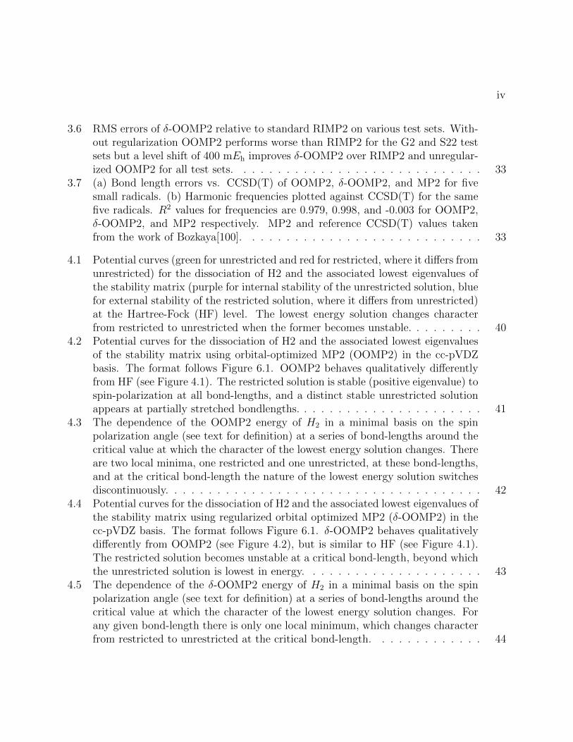
3.6 RMS errors of δ-OOMP2 relative to standard RIMP2 on various test sets. With-out regularization OOMP2 performs worse than RIMP2 for the G2 and S22 testsets but a level shift of 400 mEh improves δ-OOMP2 over RIMP2 and unregular-ized OOMP2 for all test sets. . . . . . . . . . . . . . . . . . . . . . . . . . . . . 33
3.7 (a) Bond length errors vs. CCSD(T) of OOMP2, δ-OOMP2, and MP2 for fivesmall radicals. (b) Harmonic frequencies plotted against CCSD(T) for the samefive radicals. R2 values for frequencies are 0.979, 0.998, and -0.003 for OOMP2,δ-OOMP2, and MP2 respectively. MP2 and reference CCSD(T) values takenfrom the work of Bozkaya[100]. . . . . . . . . . . . . . . . . . . . . . . . . . . . 33
4.1 Potential curves (green for unrestricted and red for restricted, where it differs fromunrestricted) for the dissociation of H2 and the associated lowest eigenvalues ofthe stability matrix (purple for internal stability of the unrestricted solution, bluefor external stability of the restricted solution, where it differs from unrestricted)at the Hartree-Fock (HF) level. The lowest energy solution changes characterfrom restricted to unrestricted when the former becomes unstable. . . . . . . . . 40
4.2 Potential curves for the dissociation of H2 and the associated lowest eigenvaluesof the stability matrix using orbital-optimized MP2 (OOMP2) in the cc-pVDZbasis. The format follows Figure 6.1. OOMP2 behaves qualitatively differentlyfrom HF (see Figure 4.1). The restricted solution is stable (positive eigenvalue) tospin-polarization at all bond-lengths, and a distinct stable unrestricted solutionappears at partially stretched bondlengths. . . . . . . . . . . . . . . . . . . . . . 41
4.3 The dependence of the OOMP2 energy of H2 in a minimal basis on the spinpolarization angle (see text for definition) at a series of bond-lengths around thecritical value at which the character of the lowest energy solution changes. Thereare two local minima, one restricted and one unrestricted, at these bond-lengths,and at the critical bond-length the nature of the lowest energy solution switchesdiscontinuously. . . . . . . . . . . . . . . . . . . . . . . . . . . . . . . . . . . . . 42
4.4 Potential curves for the dissociation of H2 and the associated lowest eigenvalues ofthe stability matrix using regularized orbital optimized MP2 (δ-OOMP2) in thecc-pVDZ basis. The format follows Figure 6.1. δ-OOMP2 behaves qualitativelydifferently from OOMP2 (see Figure 4.2), but is similar to HF (see Figure 4.1).The restricted solution becomes unstable at a critical bond-length, beyond whichthe unrestricted solution is lowest in energy. . . . . . . . . . . . . . . . . . . . . 43
4.5 The dependence of the δ-OOMP2 energy of H2 in a minimal basis on the spinpolarization angle (see text for definition) at a series of bond-lengths around thecritical value at which the character of the lowest energy solution changes. Forany given bond-length there is only one local minimum, which changes characterfrom restricted to unrestricted at the critical bond-length. . . . . . . . . . . . . 44

v
5.1 Dissociation curve of ethane in an aug-cc-pVTZ basis. 〈S2〉 of the unrestrictedsolution and lowest Hessian eigenvalue for the restricted solutions plotted to showdiscontinuity in orbitals. . . . . . . . . . . . . . . . . . . . . . . . . . . . . . . . 48
5.2 Dissociation curve of ethene in an aug-cc-pVTZ basis. 〈S2〉 of the unrestrictedsolution and lowest Hessian eigenvalue for the restricted solutions plotted to showdiscontinuity in orbitals. . . . . . . . . . . . . . . . . . . . . . . . . . . . . . . . 49
5.3 Dissociation curve of ethane in an aug-cc-pVTZ basis for σ-OOMP2 with an σvalue of 3.2. 〈S2〉 of the unrestricted solution and lowest Hessian eigenvalue forthe restricted solutions plotted to show discontinuity in orbitals. . . . . . . . . . 50
5.4 Dissociation curve of ethene in an aug-cc-pVTZ basis for σ-OOMP2 with an σvalue of 3.2. 〈S2〉 of the unrestricted solution and lowest Hessian eigenvalue forthe restricted solutions plotted to show discontinuity in orbitals. . . . . . . . . . 51
5.5 Dissociation curve of ethyne in an aug-cc-pVTZ basis for σ-OOMP2 with an σvalue of 3.2. 〈S2〉 of the unrestricted solution and lowest Hessian eigenvalue forthe restricted solutions plotted to show discontinuity in orbitals. . . . . . . . . . 52
6.1 δ-CC2 RMSE for various ground state test sets divided by RIMP2 RMSE on thesame sets for various values of δ. . . . . . . . . . . . . . . . . . . . . . . . . . . 56
6.2 Ozone symmetric dissociation curve at angle 142.76◦ for CC2 with regularizationparameters 0, 100, 150, and 200 mEh and CCSD in an aug-cc-pVTZ basis. . . . 57
7.1 Plot of 〈∆V 〉λ as a function of lambda for sampling with P = 200. R2 values forthe fits are 0.996, 0.984, and 0.998 for the monomer, dimer and sulfate clusterrespectively. . . . . . . . . . . . . . . . . . . . . . . . . . . . . . . . . . . . . . . 66
7.2 Errors in anharmonicity on a Morse potential of H2 using the free particle andharmonic propagator full energy approaches as well as thermodynamic integra-tion. The Morse potential is parameterized with De = 0.176 and a = 1.4886. . . 67
7.3 Errors in anharmonicity for H2O monomer using FFP, HOP, and TI. Referencevalues from direct grid fitting of CCSD(T) calculation[192]. . . . . . . . . . . . . 69
7.4 Errors in anharmonicity for H2O dimer using HOP and TI. The reference here isbased on CCSD(T) electronics, but only VPT2 for nuclear energies[193]. . . . . 70
7.5 Anharmonic ZPE for Sulfate 3 H2O cluster using TI. . . . . . . . . . . . . . . . 717.6 Relative Energies of Sulfate 3 H2O clusters using TI. . . . . . . . . . . . . . . . 727.7 Relative Energies of Sulfate 4 H2O clusters using TI. . . . . . . . . . . . . . . . 727.8 Relative Energies of Sulfate 5 H2O clusters using TI. . . . . . . . . . . . . . . . 737.9 Relative Energies of Sulfate 6 H2O clusters using TI. . . . . . . . . . . . . . . . 73

vi
List of Tables
2.1 Quantification of spin symmetry breaking in fullerene systems. ∆E = ERHF −EUHF and number of unpaired electrons as described in the text. . . . . . . . . . 16
2.2 Calculated Etriplet − Esinglet from restricted and unrestricted HF and MP2 com-pared to experimental literature values of C60 and C36. . . . . . . . . . . . . . . 19
5.1 Root mean square error (RMSE) in kcal/mol for σ-OOMP2 with various valuesof σ and δ-OOMP2 with the recommended parameterization of 400 mEh. . . . . 49
6.1 Excited state errors on the Thiel test set for regularized δ-EOM-CC2 vs. CC3values in TZVP and aug-cc-pVTZ basis for varying values of δ. All errors in eV. 58
6.2 Excited state errors on the Wiberg test set for regularized δ-EOM-CC2 valuesin a 6-311(3+,3+)G** basis for varying values of δ vs. accurate experimentalvalues. All errors in eV. . . . . . . . . . . . . . . . . . . . . . . . . . . . . . . . 58
7.1 Table of the number of samples required to reduce sampling error to within 5%of calculated anharmonic ZPE. . . . . . . . . . . . . . . . . . . . . . . . . . . . 68
7.2 Anharmonic ZPE for the lowest energy Sulfate-3 H2O cluster with CC-VSCF onMP2/TZP[194], TOSH and VPT2 on B3LYP/6-31+G*[179], and PIMC TI onpolarizable force field. . . . . . . . . . . . . . . . . . . . . . . . . . . . . . . . . 69

vii
Acknowledgments
I thank Ellie for supporting me in every way while working on my PhD. I thank Martin forbeing engaging when I was learning new things, open when I had ideas, and kind when Imade mistakes. I thank the group for being good colleagues, classmates, and friends; I don’tknow how I’d have made it 5 years with out you all, Paul, Sam, Eric, Yuezhi, Jules, Narbe,Nick, Jonathan, Rostam, Westin, Kristi, Evgeny, Tom, Daniel, Fran, Shaama.

1
Chapter 1
Introduction
1.1 Background
The First Question: Why?
Why do we study chemistry? We do so because it is useful and it is hard. It is useful becausechemical processes take place on the energy scale of life. Interesting molecules change fromstable to reactive depending on their environment, allowing humans to manipulate them intodifferent forms. It is hard because it takes place on a length scale that is small enough tohave no intuitive understanding by way of human senses. We can see a ball rolling, a lionhunting prey, or even an enzyme unzipping a DNA helix and we don’t need equations to atleast get a sense of what’s happening. But even seeing the density of a benzene molecule asin recent experiments gives us no intuition about its behavior and reactivity, which bringsus to the point: we can only ever understand chemistry through models.
For many years these models have been purely heuristic or quantitative but disconnected(we could measure acidity and heat of formation, but had no link between the two models).In the early 20th century, the development of quantum mechanics revolutionized our under-standing of the behavior of systems on an atomic length scale. We finally had the tools todescribe chemical processes starting from the atomic pieces of electrons and nuclei. Thisknowledge allowed us to develop assessment tools that rely on the electronic and vibrationalstructure of a molecule (spectroscopy, NMR, . . . ) rather than simple reactivity measures.
While spectra are useful, we can still (by definition really) only ever measure projectionsof the molecular wave function and can only do so for chemical systems we can access, i.e.have produced and stabilized in a measurable form and amount. The theoretician, aided byquantum theory, can now calculate the properties of molecules directly and quantitativelybut must make major approximations to do so in a tractable way. In this way, the tools ofexperimentalist and theoretician are complementary: experimentalists know that what theydo is real but can’t be sure of what they do, while computational chemists can know exactlywhat they’re modeling but not be sure of whether it’s modeling reality.

CHAPTER 1. INTRODUCTION 2
The Second Question: What?
What is quantum mechanics as it relates to molecular processes? Quantum mechanics (QM)is fundamentally different from classical mechanics (CM) in that particles are treated as fieldsto be characterized by multi-dimensional wave functions in a Hilbert spacerather than thediscrete points (xi, pi) of CM. On large size or energy scales these fields become so localizedas to be effectively points obeying CM, which is the correspondence principle. Molecularquantum mechanics is primarily governed by the Hamiltonian, given in atomic units by,
Hmol = Tn + Te + Vnn + Vne + Vee
=n∑i
1
2Mi
∇2Ri
+e∑i
1
2∇2ri
+n∑j>i
ZiZj
|Ri − Rj|−
n∑i
e∑j
Zi
|Ri − rj|+
e∑j>i
1
|ri − rj|(1.1)
The dynamics of the system are determined by the time propagator e−it~ H . Considering
the density operator, e−βH , shows that at low enough temperatures, systems will be domi-nated by the lowest eigenstate of H, the ground state, assuming excited states are higher inenergy than thermal fluctuations (which for the electronic part will almost certainly be truein standard conditions).
It is also interesting to consider molecules interacting with photons of light, which is notincluded in Hmol, but as far as this work is concerned we will focus on characterizing themolecular structure itself as a required first step to studying interactions of light and matter.
The Third Question: How?
Given Hmol for a chemical system, how do we determine the molecular wavefunction andits properties? The first approximation that we will assume for all of our modeling hereinis that the electronic states are not coupled through the kinetic energy operator–the Born-Oppenheimer approximation. We define,
Hnuc = Tn + Vnn
Hel = Te + Vne + Vee(1.2)
If we solve for the eigenvectors of Hel(r, R) over the space of electrons for given R, callthem φi(r, R) with eigenvalues Eel
i , we can without assumption write the wavefunction asa linear combination of the eigenvectors with R-dependent coefficients giving Ψ(r, R) =χi(R)φi(r, R). The approximation we make then is that,
〈φj(r, R)|Hnuc|χi(R)〉|φi(r, R)〉 = Hnuc|χj(R)〉δi,j (1.3)

CHAPTER 1. INTRODUCTION 3
Which allows for us to solve for the nuclear wavefunctions, χi(R), that give an eigenfunctionof the total Hamiltonian by projecting out the electronic part:
〈φj|Hnuc + Hel|χi〉|φi〉 = 〈φj|Etotal|χj(R)〉δi,j=⇒
(Hnuc + Eel
j (R))|χj〉 = Etotal|χj〉
(1.4)
Thus our nuclear wavefunctions are eigenfunctions of Hnuc plus a term that represents theelectronic potential energy surface. We will often neglect the quantum nature of the nucleiand simply add the nuclear repulsion to our electronic energies or account for quantumeffects through the harmonic approximation to Eel(R) to account for the fact that even thelowest energy vibrational state has zero-point energy (ZPE). We will also discuss higher levelapproximations later in this work.
Now that we’ve waved away the nuclear part of the equations for the moment, we candiscuss how we go about solving for the eigenvalues of the Hamiltonian. A simple approachis to choose a form for our wave function and minimize the energy (expectation value of H)with respect to the wavefunction parameters. This will give us an upper bound to the energyby the variational principle–since all wavefunctions can be written as linear combinations oforthogonal eigenvectors, the expectation value of an operator can be written as a weightedaverage of its eigenvalues which is always greater than or equal to the lowest such eigenvalue(assuming bounded from below). The simplest many electron wavefunction that satisfiesFermi statistics is an antisymmetrized product of one electron functions called a Slaterdeterminant.
The remaining question then is how will we construct these one electron functions? Itturns out that the realization that we should use Gaussians because it simplifies the mathe-matics was a foundational one for computational chemistry [1–3]. Now we pick a one electronbasis, the atomic orbitals or AO’s, which are combinations of radial Gaussians and sphericalharmonics that are preoptimized for chemical systems. Each occupied orbital, φi, will nowbe expressed in the basis of AO’s, χµ, as,
|i〉 = Cµi|µ〉 (1.5)
We require, without loss of generality, that the {φi} to be orthogonal and define a set ofunoccupied orbitals, {φa}, to form a complete orthogonal basis over the AO space. Thesevirtual orbitals are a formality for now but will become significant in higher level theories.The full wave function can be constructed as ψ(ri) = Det[φ(r1) . . . φ(rn)] to antisymmetrizethe wavefunction. We can now formulate the energy in matrix form by taking advantage ofthe Slater-Condon rules for inner products of determinantal forms with one and two electronoperators.

CHAPTER 1. INTRODUCTION 4
E = 〈ψ|H|ψ〉
= 〈i|T + Vne|i〉+1
2〈ij||ij〉
= hii +1
2Jii −
1
2Kii
(1.6)
Since this energy is invariant to orbital rotations within the occupied subspace, we canminimize the energy with respect to occupied virtual mixing only. Parameterizing all unitaryorbital rotations by U = eΘ where Θ is an antisymmetric matrix and taking the gradient ofE(Θ) gives:
∂E
∂θia= hia + Jia −Kia
= Fia
(1.7)
where F is the famous Fock matrix. We have now derived the Hartree-Fock (HF) methodusing a variational approach, but should note that the traditional derivation makes use of amean-field approximation where electrons are repelled by only the density of the electrons[4].These approaches give identical results; assuming independent electrons in our form for thewavefunction (excepting correlation through the antisymmetrizer) is equivalent to using amean-field coulomb potential. While the mean-field approach gives better physical intuition,the variational method dresses the mathematics in a way that shows it clearly as a nonlinearoptimization problem and invites us to consider the toolset of nonlinear optimization. Wecan implement this algorithm in O (n3) time by taking advantage of the spatial sparsity ofthe atomic orbital overlaps.
What we have left out of the previous discussion is the spin component of the electrons.As Fermions with with a spin of 1
2, electrons have a spin degree of freedom that can be
described in the basis of eigenstates of Sz, |α〉 and |β〉. The first approximation we make isthat each orbital has been projected onto either |α〉 or |β〉, and thus Slater determinants willbe eigenstates of Sz. In this unrestricted HF (UHF) approximation, single determinants arenot necessarily eigenstates of the full S2 operator–a condition that the exact wavefunctioncan meet due to S2 commuting with H. To satisfy this condition we can require that forevery α electron, we have a corresponding β electron that has the same spacial orbital. Thisnew approximation is referred to as restricted HF (RHF).
By the variational principle, each added constraint reduces the space we minimize overand thus can only raise the energy, bringing it farther from the true ground state energy,but our base wavefunction presumably is closer to the true eigenfunction in some sense asthey share the correct spin symmetry. This tension between better energetics versus spinsymmetry, referred to as the symmetry dilemma, will be fundamental to much of Chapters2-4 on symmetry breaking and orbital-optimized methods.

CHAPTER 1. INTRODUCTION 5
HF has given us an approach to optimize our one electron basis of MOs and constructa many electron function by taking the first n of them. What’s more is that we can form abasis for the n-particle Fock space by taking all possible combinations of n orbitals, or moreconstructively, view each of these determinants as an excitation from the ground state HFdeterminant, |0〉. We classify these determinants by excitation level so a state with orbitali and j replaced with a and b will be denoted as the doubly excited determinant |abij 〉.
1.2 Electron Correlation
Configuration Interaction
With only averaged Coulomb forces between electrons in the HF approach, the next levelto improve our calculations is the account for the correlations between electrons. Althoughincredibly limited in practice, we will begin our discussion of electron correlation with con-figuration interaction (CI) as a simple starting point. Given our may electron basis we’veconstructed using HF orbitals, if we want the lowest eigenvalue of H, we can simply con-struct the H matrix in a basis of our determinants and use any linear algebra approachto get the lowest eigenvalue (think of this as diagonalization but in practice something likeDavidson[5]). Since the determinants form a complete basis over the Fock space determinedby the AO’s, it actually doesn’t matter which set of MO’s we use to construct H; full CI(FCI) will always gives the exact energy for a given AO basis. So why do we need anythingother than FCI? Considering the size of H, we realize there are
(Nn
)determinants when we
have N AO’s and n electrons. This factorial growth is explosive and limits FCI to only thesmallest of atoms and diatomics.
If the full matrix is too large, why not just truncate it at some point? we can dothis and truncate at a given excitation level (i.e. CIS for singles, CISD for singles anddoubles. . . ) guided by the fact that we consider the ground state determinant to be a zerothorder approximation and thus mostly correct. While not unreasonable for small systems,the fundamental failing of truncated CI methods is their failure to be size consistent–theproperty that a method gives the same result for two noninteracting systems as it wouldfro calculating them separately. The basic idea of why CISD fails this test, is that while itcan describe double excitations on both independent molecules, when taken together, theseuncoupled double excitations are formally quadruple excitations and can’t be described inthe CISD framework.
Another way we can view CI that will more naturally extend to other correlated methodsis to view it as variationally minimizing a linearly parameterized combination of excitations.

CHAPTER 1. INTRODUCTION 6
The wavefunction can then be written,
ΨCI = (1 + T1 + T2 + · · ·+ Tn)|0〉T1 = tai a
†aai
T2 = tabij a†ba†aaj ai
(1.8)
Where Tx is the xth order excitation operator, ai destroys an electron in orbital i and a†acreates an electron in orbital a. Minimizing the expectation value of the Hamiltonian withrespect to the t-amplitudes is equivalent to finding the lowest eigenvector as before.
The first lesson we take from CI is that the more approximate the method, the moresensitive the results will be to zeroth order orbitals. The second is that the “no free lunch”idea can be seen in the a tradeoff of cost versus accuracy. A third lesson is that we wantmethods that are size consistent to allow us to describe retains where bonds are formed orbroken and to be able to apply our methods to large systems without accuracy degrading.
Coupled Cluster
Whereas the linear parameterization of the truncated CI wavefunction led to its failure todescribe independent correlations on different subsystems, coupled clusters (CC) utilizes anexponential parameterization to build the separability into the method. The CC wavefunc-tion is constructed as,
ΨCC = e(T1+T2+... )|0〉 (1.9)
Now if we truncate at double excitations (referred to as CCSD) we see that the wavefunc-tion can contain higher than double excitations (by considering the Taylor expansion), butonly as products of the singles and double excitation amplitudes. Unfortunately, attempt-ing to solve for the t-amplitudes using a variational approach leads to equations that don’ttruncate, so we solve using a projective approach . The CCSD amplitudes are solved usingthe following projected equations:
〈0|H|0〉 = ECC
〈ai |H|0〉 = 0
〈abij |H|0〉 = 0
(1.10)
Where H is the similarity transformed Hamiltonian e−(T1+T2)HeT1+T2 . We can simplify theequations by rewriting H using the Baker-Campbell-Hausdorff expansion which truncatesafter a finite number of terms. These equations can then be self-consistently iterated to solvefor the amplitudes. To really make sense of CC we recommend learning about diagrammaticrepresentations[6, 7] of the equations but do no use them here.
CHAPTER 1. INTRODUCTION 7
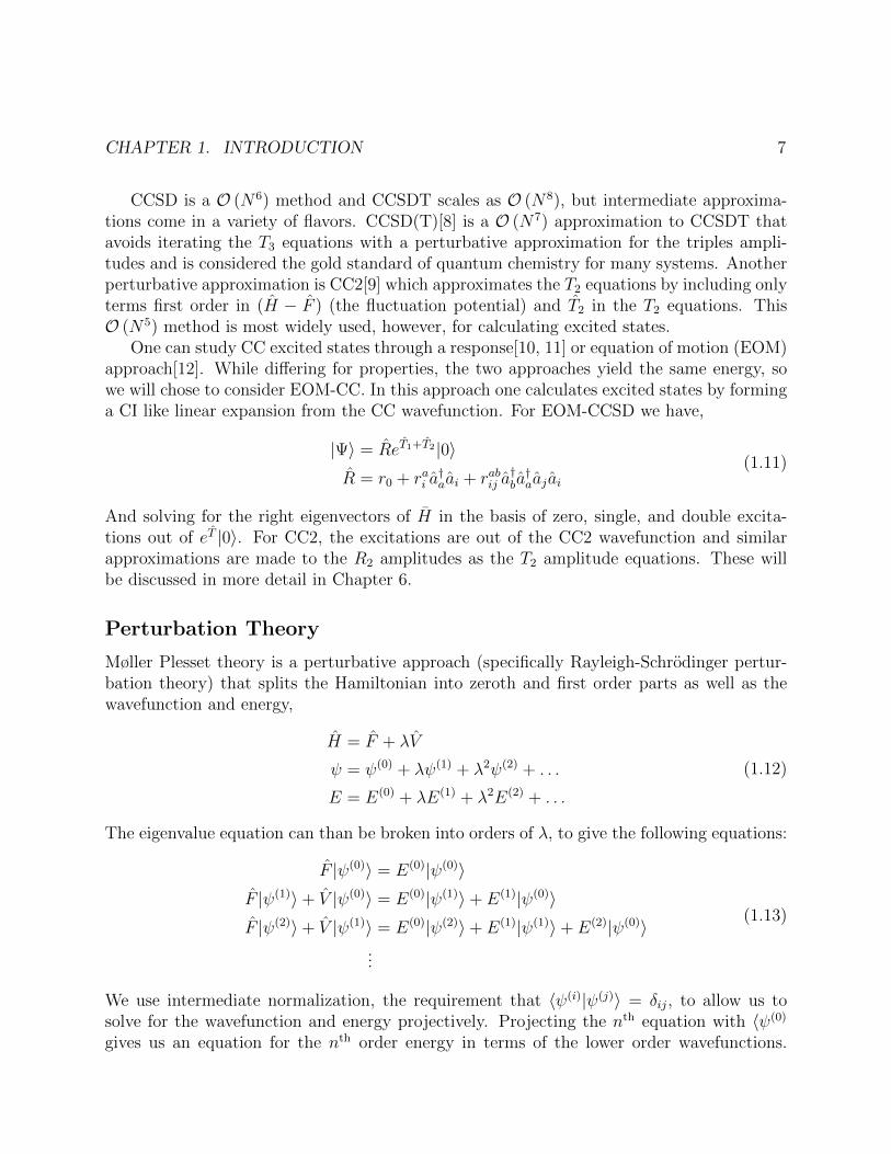
CCSD is a O (N6) method and CCSDT scales as O (N8), but intermediate approxima-tions come in a variety of flavors. CCSD(T)[8] is a O (N7) approximation to CCSDT thatavoids iterating the T3 equations with a perturbative approximation for the triples ampli-tudes and is considered the gold standard of quantum chemistry for many systems. Anotherperturbative approximation is CC2[9] which approximates the T2 equations by including onlyterms first order in (H − F ) (the fluctuation potential) and T2 in the T2 equations. ThisO (N5) method is most widely used, however, for calculating excited states.
One can study CC excited states through a response[10, 11] or equation of motion (EOM)approach[12]. While differing for properties, the two approaches yield the same energy, sowe will chose to consider EOM-CC. In this approach one calculates excited states by forminga CI like linear expansion from the CC wavefunction. For EOM-CCSD we have,
|Ψ〉 = ReT1+T2 |0〉R = r0 + rai a
†aai + rabij a
†ba†aaj ai
(1.11)
And solving for the right eigenvectors of H in the basis of zero, single, and double excita-tions out of eT |0〉. For CC2, the excitations are out of the CC2 wavefunction and similarapproximations are made to the R2 amplitudes as the T2 amplitude equations. These willbe discussed in more detail in Chapter 6.
Perturbation Theory
Møller Plesset theory is a perturbative approach (specifically Rayleigh-Schrodinger pertur-bation theory) that splits the Hamiltonian into zeroth and first order parts as well as thewavefunction and energy,
H = F + λV
ψ = ψ(0) + λψ(1) + λ2ψ(2) + . . .
E = E(0) + λE(1) + λ2E(2) + . . .
(1.12)
The eigenvalue equation can than be broken into orders of λ, to give the following equations:
F |ψ(0)〉 = E(0)|ψ(0)〉F |ψ(1)〉+ V |ψ(0)〉 = E(0)|ψ(1)〉+ E(1)|ψ(0)〉F |ψ(2)〉+ V |ψ(1)〉 = E(0)|ψ(2)〉+ E(1)|ψ(1)〉+ E(2)|ψ(0)〉
...
(1.13)
We use intermediate normalization, the requirement that 〈ψ(i)|ψ(j)〉 = δij, to allow us tosolve for the wavefunction and energy projectively. Projecting the nth equation with 〈ψ(0)
gives us an equation for the nth order energy in terms of the lower order wavefunctions.

CHAPTER 1. INTRODUCTION 8
Projecting with excited determinants allows us to solve for the wavefunctions. To calculatethe energy up to second order (MP2) we have,
E(0) + E(1) = 〈0|F + V |0〉= EHF
(1.14)
|ψ(1)〉 =〈abij |V |0〉
E(0) − 〈abij |F |abij 〉|abij 〉
=〈ij||ab〉
εi + εj − εa − εb|abij 〉
(1.15)
E(2) = 〈0|V |ψ(1)〉
=|〈ij||ab〉|2
εi + εj − εa − εb(1.16)
Where we have used that fact that the for HF orbitals Fia = 0 and we can diagonalize theoccupied and virtual blocks of F to give diagonal elements εp. This give us a O (N5) methodthat performs well for closed-shell molecular energies, geometries, and frequencies. Theproblems of MP2 that can occur when orbital symmetry breaking takes place for open-shellsystems or aromatic molecules will be further studied in Chapters 2-4.
1.3 Statistical Quantum Thermodynamics
Even if electronics are solved for exactly they are still only part of the story. As discussedpreviously, the Born-Oppenheimer approximation allows us to separate the electronic prob-lem from the nuclear problem, but not neglect it entirely. While nuclear contributions tendto be smaller and thus merit weaker approximations, often the harmonic level is not enough.One option is to study vibrations using a path integral (PI) formulation that allows us toturn problems of quantum mechancis into coupled classical thermodynamic problems[13, 14].
We begin with a fundamental quantity of thermodynamics, the partition function Q. Wecan translate the classical sum over states to the quantum trace over density operator and

CHAPTER 1. INTRODUCTION 9
see how expectation values work in the quantum context in the following equations,
Q =∑i
e−βEi
Q =∑i
〈ψi|e−βH |ψi〉
Q = Tr e−βH
〈A〉 =Tr Ae−βH
Tr e−βH
〈H〉 = − d
dβlnQ
(1.17)
Where β is the inverse temperature. We get the path integral formulation by representingthe trace in a spatial coordinate basis and inserting P − 1 sets of the identity,
Q = Tr e−βH
Q =
∫dx1 〈x1|e−βH |x1〉
Q =
∫. . .
∫dx1 . . . dxP 〈x1|e−
βPH |x2〉 . . . 〈xP |e−
βPH |x1
(1.18)
If βP
is small enough, we can use a high temperature approximation to these density matrixelements by treating them with some zeroth order Hamiltonian,
e−βP
(H0+∆V ) = e−βPH0e−
βP
∆V +O
((β
P
)3 [Ho,∆V
])
Q ≈∫. . .
∫dx1 . . . dxP
P∏i
〈xi|e−βPH0|xi+1〉〈xi|e−
βP
∆V |xi+1〉
Q ≈∫. . .
∫dx1 . . . dxP
P∏i
〈xi|e−βPH0|xi+1〉e−
βP
∆V (xi)
(1.19)
If we select H0 = T , the free particle approximation, we get a partition function thatcorresponds to a classical polymer of P systems connected to their neighbors with harmonicpotentials simulated at a temperature P
β. In chapter 7 we will discuss how using a better H0
can improve our results for calculating vibrational anharmonicities.
1.4 Outline
This thesis is organized as follows.

CHAPTER 1. INTRODUCTION 10
Chapter 2
The ground state restricted Hartree Fock (RHF) wave function of C60 is found to be unstablewith respect to spin symmetry breaking, and further minimization leads to a significantlyspin contaminated unrestricted (UHF) solution (〈S2〉 = 7.5, 9.6 for singlet and triplet respec-tively). The nature of the symmetry breaking in C60 relative to the radicaloid fullerene, C36,is assessed by energy lowering of the UHF solution, 〈S2〉, and the unpaired electron number.We conclude that the high value of each of these measures in C60 is not attributable to strongcorrelation behavior as is the case for C36. Instead, their origin is from the collective effectof relatively weak, global correlations present in the π space of both fullerenes. Second orderperturbation (MP2) calculations of the singlet triplet gap are significantly more accuratewith RHF orbitals than UHF orbitals, while orbital optimized opposite spin second ordercorrelation (O2) performs even better.
Chapter 3
Orbital optimized second order perturbation theory (OOMP2) optimizes the zeroth orderwave function in the presence of correlations, removing the dependence of the method onHartree–Fock orbitals. This is particularly important for systems where mean field orbitalsspin contaminate to artificially lower the zeroth order energy such as open shell molecules,highly conjugated systems, and organometallic compounds. Unfortunately, the promise ofOOMP2 is hampered by the possibility of solutions being drawn into divergences, which canoccur during the optimization procedure if HOMO and LUMO energies approach degeneracy.In this work, we regularize these divergences through the simple addition of a level shiftparameter to the denominator of the MP2 amplitudes. We find that a large level shiftparameter of 400 mEh removes divergent behavior while also improving the overall accuracyof the method for atomization energies, barrier heights, intermolecular interactions, radicalstabilization energies, and metal binding energies.
Chapter 4
Following the lowest eigenvalue of the orbital-optimized second order Møller-Plesset pertur-bation theory (OOMP2) hessian during H2 dissociation reveals the surprising stability of thespin-restricted solution at all separations, with a second independent unrestricted solution.We show that a single stable solution can be recovered by using the regularized OOMP2method (δ-OOMP2), which contains a level shift.
Chapter ??
Previous work[15] established the unexpected behavior of orbital-optimized second-orderperturbation theory (OOMP2) for bond dissociations wherein orbitals could change discon-

CHAPTER 1. INTRODUCTION 11
tinuously at the unrestriction point. Level-shift regularization (δ-OOMP2) was able to fixthe problem for H2 but we find this solution does not generalize to even other single bond dis-sociations. We implement a new regularization approach (σ-OOMP2) based on Evangelista’ssimilarity renormalization group theory[16] that we show to be more robust for describingeven triple bond dissociations.
Chapter 6
We extend the family of semi-empirically modified methods based on the introduction of aregularization parameter to ground and excited state CC2. It is found that a value of 150mEh reduces errors in energies across a broad spectrum of ground state chemical test setsand corrects the reported failure of CC2 for ozone. Similarly, a value of 150 mEh balancessystematic errors for valence and Rydberg excited states in small molecule test sets. Basedon the apparent robustness of these results we suggest the consideration of δ-CC2 as asemi-empirical, trivially modified CC2-based method.
Chapter 7
Electronic structure theory results are often limited in accuracy by their description of vi-brational errors, which are challenging to calculate beyond the harmonic approximation.To calculate anharmonic vibrational energy corrections for low temperature molecules andclusters with systematically reducible errors, we propose a novel combination of using ther-modynamic integration and a static harmonic propagator for path integral Monte Carlo.The method requires only electronic single point calculations for sampling as opposed togradients or Hessians (beyond an initial frequency calculation), and requires a much smallernumber of beads and steps due to its use of a more appropriate zeroth order approximationto the propagator. The method is applied to toy systems as well as reassessing the globalminimum energy structure of low temperature sulfate-water clusters.
1.5 Additional Work
In addition to the chapters listed above, some work has not made it into the thesis (mostlydue to the papers being written in Word rather than LaTex. . . ). Most notably, my workin collaboration with the Long group, modeling molecular organic frameworks (MOF) andtheir application for hydrogen storage. We published a paper comparing our models to thecite specific binding energies they got from temperature dependent IR on H2 in a BTTMOF[17]. We benchmarked our binding enthalpies against experimental numbers showinggood agreement, and looked at metal and ion substituted MOFs. Our prediction that Brwould make a stronger binding compound was confirmed after publication, but was notstudied further do to dangerous steps in synthesis due to the Br.

CHAPTER 1. INTRODUCTION 12
A second project with the Long group involved trying to understand the differentialbinding of H2 in MOFs that only differed by an isomerization in the organic linker[18].Modeling MOF-74 is difficult due to metal chains down the framework, but we did our bestto create a model that isolated the differences in the linker by capping metals with CO andfreezing them into experimental geometries. Our work showed a combination of increasedelectrons on the metal and an extra interaction with the ring present in only one isomer tobe creating higher binding in the meta variant.
Last I just wanted to document some work that never went anywhere do to convergenceissues and early discouraging results. I proposed using orthogonalized Hartree product or-bitals[19, 20] as a way to avoid artificial spin symmetry breaking for radicals and aromaticcompounds. The hypothesis was that since artificial spin symmetry breaking could be causedby HF using Fermi correlation (from the antisymmetrization of the wavefunction) to com-pensate for a complete lack of Coulomb correlation. Whereas OOMP2 tries to account forCoulomb correlation in the optimization process to achieve balance, another option could beto just get rid of Fermi correlation by using Hartree product orbitals. The first problem isthat they are not invariant to occupied-occupied rotations which makes the non-linear opti-mization process a huge pain. The second problem is that it appears that spin contaminatedsolutions still appear and were probably the global minima (although not for certain due todifficulty converging solutions); this may still be happening due to localization since we’renot allowing for Fermi correlation.

13
Chapter 2
On the Nature of ElectronCorrelation in C60
2.1 Introduction
Quantum chemists strive to model realistic chemical systems with a high degree of accu-racy. The problem is that accurate methods such as multireference configuration interaction(MRCI) and even single reference coupled cluster methods such as CCSD(T) become rapidlyunfeasible as system size increases[8, 21]. For this reason, whenever possible we would preferto take advantage of simpler, single determinant methods such as Hartree Fock (HF)[22] ordensity functional theory (DFT)[23, 24]. To that end, we would like to first approximate thesystem as well as possible within the space of HF methods and second to gain some insightinto when our approximations will be valid.
By allowing different orbitals for different spins, unrestricted Hartree Fock (UHF)[25]can improve upon the energy of spin restricted HF (RHF). UHF thus incorporates somecorrelation between electrons of opposite spin in a single determinant wave function[26, 27]as a result of permitting spin contamination[28]. This increase in the expectation value ofthe total spin squared operator is due to the breaking of spin symmetry and the presence ofhigher spin states in the solution[29]. Although spin contamination is an unphysical aspectof the UHF wavefunction, it may imply that there is static correlation present in the system.By static correlation, we mean that the lowest energy HF (i.e. UHF) wave function is notan appropriate zero order wave function, and thus cannot be satisfactorily corrected by e.g.low order perturbation theory.
A simple but illustrative case of spin symmetry breaking is the dissociation of H2 into twoH atoms[4]. RHF is insufficient, and dissociates H2 into a superposition of 2 H and H+ + H–.Allowing for the unrestriction of the spin orbitals leads to the correct products; however, asthe bond length increases beyond the equilibrium value, at a certain point, 〈S2〉 becomesincreasingly contaminated up to a final value of 1 due to the wavefunction becoming a linear

CHAPTER 2. ON THE NATURE OF ELECTRON CORRELATION IN C60 14
combination of a singlet and triplet.The energy is exact at dissociation (“asymptotic regime”), indicating that spin contam-
ination is not necessarily a serious problem. The more challenging region of the surface isthe so-called “recoupling regime” at bond lengths where the RHF solution is no longer theglobal minimum, but before the asymptotic regime is reached. This is the region where,unlike the equilibrium geometry, static correlation is becoming important, but unlike the“asymptotic regime,” the correlation energy is nonzero.
As opposed to RHF, in a broken spin symmetry UHF solution, the natural orbitalscan have fractional occupation numbers leading to a picture of a molecule with polyradicalbehavior. Measures of the extent of spin symmetry breaking should thus be signals ofpolyradical nature in a system. For example 〈S2〉 has been correlated to polyradicalismin polyacenes[30]; as the length of the acene increases, the singlet-triplet gap decreasesand the spin contamination increases. Another study on the acenes used density matrixrenormalization group theory to correlate the π space and showed the polyradicalism of thelarger acenes through unpaired electron number as well as various correlation functions [31].
A more complex example of a polyradical and likely strongly correlated system is theground state of the fullerene, C36. On the experimental side, it has been found from NMRthat solid C36 is of D6h symmetry due to the single peak present in the C13 spectra[32]. Onthe computational side, however, there has been significant discrepancy between differentelectronic structure methods on the optimized geometry[33–37] and even multiplicity[37, 38]of the ground state of this small fullerene.
One explanation for the failing of simple methods to give the fully symmetric D6h sym-metry is given by Fowler et al [39]. Their semi-empirical CI-based estimations of correlationenergy in the isomers of C36 show that the D6h symmetry structure has a significantly largercorrelation energy than any other isomer. They argue that methods which neglect the corre-lation, such as restricted HF (and perhaps restricted DFT with inexact functionals) thereforefalsely give lower energies for the geometries with less correlation and thus misrepresent themas being similar in energy to the D6h isomer.
Another computational study on C36 has found that the RHF ground state is unstablewith respect to UHF leading to a spin contaminated solution[37]. This spin contaminationhas been seen as an indicator of the presence of radicaloid character in the electronic structureof the ground state, which would in turn emphasize the importance of using a higher levelof theory than basic RHF for its description.
Based on the interesting nature of the HF results for the radicaloid C36, herein we investi-gate the larger, and experimentally more stable fullerene, C60, for similarities and differencesin the Hartree-Fock descriptions of their ground state, and therefore the comparative char-acter of electron correlations in the two fullerenes.

CHAPTER 2. ON THE NATURE OF ELECTRON CORRELATION IN C60 15
2.2 Results and Discussion
HF calculations were run using QCHEM 3.0[40] with a 6-31G* basis and all geometries wereoptimized at the HF level of theory used for energies; for the purposes of this communicationRHF implies restricted closed shell HF for singlets and restricted open shell HF for tripletcalculations.
The first surprise for C60, considering its molecular stability, is the discovery that theRHF ground state, although a minimum in the restricted space, is unstable with respectto UHF orbital rotations. This finding brings up the question of the extent of electroncorrelations in the relatively stable C60 as compared to the radicaloid C36. Several metricsare used to compare the nature of the spin symmetry breaking in the two systems.
The first metric used is the energy lowering due to breaking of spin symmetry defined as∆E = ERHF−EUHF. As can be seen from the variational principle, this difference must be anonnegative value, but the extent can give us a way to quantify the energetic gain from spinsymmetry breaking. The second is 〈S2〉 which shows the extent of contamination by higherspin states. Of course, bearing in mind the simple H2 example discussed in the introduction,neither of these measures by themselves can conclusively indicate whether the correlationsare of the strong static type (“recoupling regime”) or not (e.g. “asymptotic regime”).
The next metric considered is the number of unpaired electrons. In restricted frameworks,the number of unpaired electrons is constrained to be an integer; however, in UHF there isno single definition for the number of unpaired electrons in, say, a singlet polyradicaloid. Forthe purposes of this paper, we will choose the definition given by Head-Gordon[41]:
nU =M∑i=1
min(ni, 2− ni)
where ni is the ith natural orbital occupation number (NOON) and M is the dimension ofthe one particle basis. This definition is chosen for its straightforward interpretation andcorrect bounds on the maximum number of unpaired electrons.
The value for each metric in the case of the two fullerenes has been compiled in Table 2.1and we now look at the first two rows to analyze the spin symmetry breaking in C60. Eachmetric gives results which are, at least on first inspection, quite dramatic. The energyis lowered by a value even larger than the RHF singlet-triplet gap of 55 kcal/mol! Thesinglet and triplet values of 〈S2〉 are both about 7.5 higher than they should be, and thereare about 9 more unpaired electrons than RHF. Do these data, particularly the unpairedelectron numbers, indicate that C60 may be a strongly correlated molecule?
We next look to C36, a system that is more definitively considered to be strongly corre-lated[33, 34, 37, 38]. When comparing the two systems it is important to take into consid-eration their size, since C60 has almost twice as many π electrons as C36. In light of thisfact, viewing Table 2.1 shows the two fullerenes have similar values of spin contaminationby looking at the 〈S2〉 values, but in terms of unpaired electrons per C atom (or π electron),

CHAPTER 2. ON THE NATURE OF ELECTRON CORRELATION IN C60 16
∆E (kcal/mol) 〈S2〉 Unpaired e−
C60 singlet 59.62 7.5 8.8triplet 85.77 9.6 10.6
C36 singlet 180.88 7.7 9.9triplet 124.59 8.7 10.2
Table 2.1: Quantification of spin symmetry breaking in fullerene systems. ∆E = ERHF −EUHF and number of unpaired electrons as described in the text.
1C36 (0.28 e−/C) shows nearly twice as many as 1C60 (0.15 e−/C). In terms of energy low-ering, the difference is even more dramatic: the RHF-UHF energy lowering is 5 kcal/mol/Cfor 1C36, but only about 1 kcal/mol/C for 1C60.
When analyzed more carefully, the 〈S2〉 and unpaired electron numbers for the twofullerenes show an important difference. While the 〈S2〉 values are very large in both cases,for C60, the difference between triplet and singlet is about two, which is the correct difference.In C36, however, the difference is only one. Likewise, for unpaired electrons the difference ofabout two for C60 is the correct one for a triplet versus a singlet state, but in C36 the numberof unpaired electrons in singlet and triplet are nearly identical. We see then, that while inC60 the behavior of the triplet relative to the singlet is preserved upon spin unrestriction,in C36 spin symmetry breaking gives us a picture of nearly equally occupied HOMO andLUMO, characteristic of strongly correlated systems.
We can gain more insight into the nature of the unpaired electrons by looking directly atthe NOON of the two systems shown in Figure 2.1. There are a couple of interesting thingsabout this plot. First, we see that in both systems, the entire π space is at least partiallyspin polarized. Thus spin polarization is a collective phenomenon in both fullerenes. Itis therefore nearly certain that spin polarization will occur in all larger fullerenes as well.Second, there is a large difference in the extent of unpairing in C60 compared to C36. Weknow from the number of unpaired electrons that there should be nearly twice the number ofunpaired electrons per carbon in C36, but this plot shows that C60 doesn’t have any naturalorbitals that are actually half occupied, while C36 has the HOMO and LUMO both withoccupation number of nearly one. Apart from this pair, the C36 and C60 NOON distributionslook qualitatively similar. We thus expect to see at least two strongly correlated electronsin C36.
Another way to look at this unpairing is to plot the unpaired electron density. We canextend the idea of unpaired electrons to an unpaired electron density by adding densitiesof natural orbitals weighted by unpaired electron number. Likewise, we can create a spindensity that is the difference between α and β densities. Figure 2.2 shows plots of theunpaired electron density, colored by the value of the spin density (light gray indicatingexcess α and dark gray excess β) of singlet and triplet C36 and C60.
These plots show global spin polarization of the entire π space. Rather than seeing 4

CHAPTER 2. ON THE NATURE OF ELECTRON CORRELATION IN C60 17
Figure 2.1: Natural orbital occupation numbers of UHF spincontaminated singlets for C36
and C60. Orbitals are numbered as a fraction of the total π space (i.e. i36
or i60
for the ith πorbital of C36 or C60 respectively).
or 5 localized areas of spin polarization as might be suggested by the value of 8.8 unpairedelectrons, the entire π space polarizes. Similar results have been found in studies on graphenefragments[42–44], but with the key distinction that spin polarization primarily takes placeon the edge carbons, which are bonded to hydrogens. In fullerenes, there are no edge sitesso the entire molecule spin polarizes with an antiferromagnetic pattern that is frustrated bythe presence of pentagons.
To further confirm the idea that C36 is strongly correlated while C60 is not, we haverun CASSCF calculations using GAMESS [45] on C36 and C60 with [6,6] and [10,8] activespaces respectively chosen based on orbital symmetries. For C60 only one configuration gavesignificant weight and the HOMO and LUMO occupation numbers are nearly 2 and 0. Theresults for C36 on the other hand show significant static correlation and occupation numbersof 1.21 and 0.79 for HOMO and LUMO. These results are interesting in two ways. First, theyqualitatively support the greater unpairing seen in the UHF wave function for C36 versusC60. Second, they do not support the observation of other NOON values larger than 0.5 seenin the UHF calculations for both C36 and C60.
We may therefore conclude that the relative behavior of the highly spin contaminatedUHF wave functions for C36 versus C60 should alert us to differences in correlations in theπ space of C36 and C60. However, from the second observation above, we do not have aclear picture of whether the UHF wave functions are particularly “better” than the RHF

CHAPTER 2. ON THE NATURE OF ELECTRON CORRELATION IN C60 18
Figure 2.2: Unpaired electron density of singlet (top) and triplet (bottom) C60 (left) andC36 (right) plotted at isovalue 0.006 A−3, with shading determined by the sign of the spindensity as described in the text.
ones. The UHF energies are certainly much lower than the RHF ones, but RHF is a propereigenfunction of S2. This is simply the much discussed symmetry dilemma[28], and thereforefurther assessment is needed.
To gain some insight into the comparative quality of the two HF wave functions forthe two fullerenes, we will consider how they handle the singlet-triplet gap, an observableproperty that typically depends significantly on correlation. This assessment can be guidedby good gas phase experimental values for C60 from phosphorescence in rare gas matrices[46]and approximate numbers for C36 from anion photoelectron spectroscopy[47].
From Table 2.2 we see that for C60 UHF gives a significantly better singlet triplet gapthan RHF. While RHF substantially overestimates the gap by about 18 kcal/mol, UHFunderestimates it by less than 8 kcal/mol. What is more surprising is that for C36, RHFactually predicts a triplet ground state, whereas UHF at least gives the sign of the singlettriplet gap correctly. However the magnitude of the singlet-triplet gap errors are nearly equalfor both RHF and UHF for C36.
One explanation of this improvement is that the spin polarization is not just a spuriousby-product brought about by the mathematical formalism, but can give a better descriptionof properties (within the HF regime) by capturing part of the true electron correlation effect.This correlation is Hollett and Gill’s “Type A” static correlation[27] and, as Fukutome claims,can contain information about the spin correlation[26].
To confirm that the presence of spin contamination is not significantly due to basis setincompleteness, we have also calculated the spin contaminated singlet state of C60 in the

CHAPTER 2. ON THE NATURE OF ELECTRON CORRELATION IN C60 19
Singlet-Triplet Gap (kcal/mol)C60 RHF 55.16
UHF 29.01RMP2 43.28UMP2 80.20
O2 34.6Experimental[46] 36.95± 0.02
C36 RHF -21.29UHF 35.00
RMP2 18.26UMP2 26.33
O2 22.07Experimental[47] ∼ 8
Table 2.2: Calculated Etriplet−Esinglet from restricted and unrestricted HF and MP2 comparedto experimental literature values of C60 and C36.
6-311G(2df) basis. At twice the basis size, we computed 〈S2〉 = 7.4, a value similar enoughto the small basis that we can be confident that the basis set is not of key importance in ourresult.
With the discovery of the spin contaminated UHF solution for C60 we are left with thedifficult question of how to move forward to post-HF methods on these large molecules.It is well known that spin contaminated UHF orbitals typically recover significantly lesscorrelation energy than RHF orbitals at the MP2 level[48], but at the same time, spincontamination is an indicator of the poor quality of RHF orbitals. Table 2.2 shows how thetwo versions of MP2 handle the singlet-triplet gap of C36 and C60. For C60, RMP2 reducesthe error of RHF by a factor of three to 6 kcal/mol. By contrast, UMP2 for C60 using thespin contaminated orbitals performs characteristically poorly, actually increasing the error.
One way forward is to use a method that does not rely on the quality of HF orbitals,but reoptimizes them in the presence of electron correlation. Brueckner coupled clustermethods[49–51] would be ideal, but are presently too expensive for routine application toproblems of this size. A less computationally demanding alternative is orbital optimizedscaled opposite spin MP2 (O2)[52]. The O2 method is found to give the same results forC60 whether initialized with RHF or spin contaminated UHF orbitals – yielding closed shellorbitals for the singlet and nearly uncontaminated orbitals for the triplet. For C60, O2 givesa reasonably accurate singlet-triplet gap result (within 2.4 kcal/mol or 7% of experiment),improving on RMP2.
The MP2 and O2 results also give us more insight into the nature of correlation inC60. The success of second order perturbation theory on observable properties using eitherrestricted or optimized orbitals shows that strong correlation, which require multiple deter-

CHAPTER 2. ON THE NATURE OF ELECTRON CORRELATION IN C60 20
minants to describe, must not be present in C60. The signs of strong correlation—very highspin contamination and unpaired electron number—must in fact be attributable to relativelysmall (on a per atom scale) but global electron correlations in the π space.
For C36 on the other hand, none of the MP2 methods, including O2, give an accuratevalue for the singlet-triplet gap and one must go to multireference MP2 to get values thatmatch experiment[37]. For a strongly correlated system such as this one, it is as expectedthat to properly describe the system, we would need to use a method with more than oneSlater determinant as the reference, or relatively high order single reference coupled clustertheory.
This distinction between the two fullerenes can be made more clearly by analyzing theNOONs resulting from the O2 calculations as shown in Figure 2.3. We can see that theunpaired nature of C60’s π space has been tamed by stabilizing the orbitals with respect tothe MP2 correlation. C36 on the other hand still has its highest occupied orbital significantlyunoccupied. These data give further support to the CASSCF results showing major staticcorrelation present only in C36.
Figure 2.3: Natural orbital occupation numbers from O2 calculations on singlet C36 and C60.Orbitals are numbered as a fraction of the total π space.

CHAPTER 2. ON THE NATURE OF ELECTRON CORRELATION IN C60 21
2.3 Conclusion
Perhaps surprisingly, we have found the RHF ground state of the very stable C60 moleculeto be unstable with respect to spin symmetry breaking, and have compared the nature ofits spin polarization to that of the much less stable fullerene, C36. From the analysis of thenumber of unpaired electrons and 〈S2〉 we are left with the picture of a global π correlationpresent in both fullerenes but with the addition of at least two strongly correlated electronsin C36. The global correlation is responsible for the spin polarization of the whole π spaceseen in Figure 2.2, the large value added to 〈S2〉, and the number of unpaired electrons.This correlation serves as a background to the strong correlation in C36 which is seen inthe additional spin polarization energy and bringing together of 〈S2〉 and unpaired electronnumber for the singlet and triplet.
These results form an interesting case study on the issues associated with simple Hartree-Fock based calculations on molecules with extended π systems. Even stable molecule likeC60 can have unstable RHF solutions due to an aggregate of weaker correlations, leadingto dramatically different, lower energy, UHF solutions. However, it is clear that large 〈S2〉values do not necessarily imply the presence of strong, static correlations, and performingMP2 from the RHF orbitals is clearly preferable to using UHF orbitals. It is still better touse correlation optimized orbitals, as in the O2 method[52].

22
Chapter 3
Regularized Orbital-Optimized MP2
3.1 Introduction
The simplest wave function ansatz that satisfies Fermi statistics is an antisymmetrized prod-uct of single electron orbitals: the Slater determinant. The Hartree–Fock (HF) method—defined by variationally minimizing the expectation value of the Hamiltonian within theSlater determinant ansatz—gives a mean-field description that obtains approximately 99%of the total energy but ultimately fails at describing most chemical processes, such as reac-tion energies, with any reasonable accuracy[22]. Excepting cases of strong/static correlation,where multi-reference methods are required to properly describe the physics, a primary as-sumption in electronic structure theory is that the HF method is a good zeroth order approx-imation for the true wave function. Møller–Plesset perturbation theory (MP), configurationinteraction, and coupled cluster (CC) theories typically use HF orbitals as the starting pointfor building up to a more accurate wave function.
Unfortunately, the assumption that HF orbitals are a good zeroth order approximationdoes fail, particularly in the case of significant spin contamination. Restricted HF (RHF)follows our chemical intuition that electrons are paired by requiring alpha and beta elec-trons to have the same spatial orbitals. Removing this requirement leads to unrestrictedHF (UHF)[25], which allows for extra variational degrees of freedom that potentially lowerthe energy but lead to other unintended consequences. The most clear implication of thisunrestriction of the wavefunction is the introduction of spin contamination, indicating thatthe wavefunction is no longer an eigenfunction of the spin squared operator[28]. While onemight not be too concerned about getting the total spin of the wavefunction correct since theenergy has no direct dependence on spin degrees of freedom, such broken symmetry solutionstypically lead to very poor zeroth order wavefunctions for MP2 and CC theories[48, 53–55].
The point is made quite clearly in the dissociation of the lithium dimer where MP2using UHF orbitals dissociates correctly but gives a very poor description of the groundstate potential, while RHF orbitals lead to the correct equilibrium behavior but dissociate

CHAPTER 3. REGULARIZED ORBITAL-OPTIMIZED MP2 23
wildly incorrectly (Figure 3.1). Artificial spin symmetry breaking occurs on a larger scale inC60, leading UMP2 to fail at describing properties such as the single-triplet gap[56]. Spincontamination also leads to total delocalization of solitons in neutral polyenyl chains thatexperimentally are known to be localized over about 18 carbon atoms[57]. These examplesillustrate the need for post-HF methods that are not tied to HF orbitals.
One such option is approximating the Brueckner orbitals—defined as the orbitals thatgive a ground state determinant with maximal overlap with the exact wave function or equiv-alently, the orbitals for which there are no single excitations in full configuration interaction(FCI) wavefunction[58]. Within the framework of FCI, one can calculate the Bruecknerorbitals using either a projective or variational approach[59]. In the projective approach,one would calculate singles amplitudes as a function of orbital rotations and minimize themto zero. For the variational approach, we constrain the singles amplitudes to be zero andminimize the CI energy with respect to orbitals, which gives the Brueckener orbitals (sincethey satisfy the constraint by construction). While these two approaches are identical in theFCI limit, introducing truncations to the CI expansion will lead to two distinct methods.
These Brueckner orbital methods can also be applied to the size-consistent exponentialansatz of coupled-cluster approximations, although they are not exact in the full limit[60].The projective approach has been implemented for CCSD as Brueckener doubles (BD)[49, 50]with the variational approach implemented for CCSD as orbital-optimized doubles (OD)[61]and for Møller Plesset theory as orbital-optimized MP2 (OOMP2)[52] and OOMP3[62].While minimizing a non-variational method may sound troubling, the value being minimizedis actually a constrained energy where the single’s contribution is set to zero, penalizingorbital solutions which have large singles contributions to the full energy.
Many of the failings of HF orbitals can be mitigated by the use of approximate Bruecknerorbital methods. Spin contamination is generally removed or significantly reduced leadingto spin eigenfunctions without resorting to restricted constraints[52, 56, 59, 63]. In additionto rectifying spin properties, the use of approximate Brueckner orbitals has been shownto improve the description of bond lengths, frequencies, and relative energies of open shellsystems[51, 52, 59, 61, 63, 64]. The use of the variational approach garners additionalbenefits due to the fact that the energy is made stable to orbital rotations. This fact givesrise to a Hellmann-Feynmann condition, simplifying response properties of the wavefunctionand removing first derivative discontinuities present in UMP2 at the unrestriction point[65].
MP2 is the one of the simplest computational methods to account for electron correlationand naturally includes long-range dispersion interactions[4]. It is ab initio, systematically im-provable, and an important alternative to the more commonly used density functional theory(DFT) in cases where DFT self-interaction error is present[66]. For these reasons, OOMP2is an important method to accurately model large, open-shell systems such as radicals ororganometallic compounds, striking a balance between the speed of HF and the accuracyof CCSD. For the case of Li2 dissociation, it connects the spin pure equilibrium descriptionto the unrestricted asymptotic limit as seen in Figure 3.1. Recently, variants of OOMP2have been proposed that use a Thouless expansion representation of OOMP2[67] along with

CHAPTER 3. REGULARIZED ORBITAL-OPTIMIZED MP2 24
another approach to orbital-optimization based on a one particle operator approximation tothe MP2 energy[68].
Figure 3.1: Li2 dissociation curve for MP2 using restricted and unrestricted orbitals and forOOMP2 with a cc-pVDZ basis. RMP2 dissociates incorrectly and UMP2 distorts the equi-librium description while OOMP2 gets the best of both worlds by continuously connectingthe two regimes, albeit with a kink due to a slight discontinuous change to the orbitals uponunrestriction.
While enabling many improvements to traditional MP2, OOMP2 brings with it the loom-ing concern of energy divergence. Inherent in Rayleigh-Schrodinger perturbation theory isthe divergence for zeroth order states with nearly degenerate energies, which translates inMP2 to divergence as the HOMO-LUMO gap goes to zero. While there are classes of post-Kohn Sham theories that can properly describe small band gap systems such as RPA[69,70] and GW theory[71, 72], in small molecular systems such a degeneracy in the HF or-bital energies is a key indicator of the presence of static correlation requiring multireferencetechniques rather than MP2.
For OOMP2, on the other hand, these divergences do not need to be present in the orbitalsused to calculate the final energy to cause problems; due to the non-variational nature of theconstrained energy, the method must only come across one of these mathematical artifactsduring the optimization procedure to keep from finding a truly stable set of orbitals. Inthis case, by removing divergences, one could properly converge to a set of orbitals that donot contain orbital degeneracies. Thus, unlike standard MP2, the divergences present in

CHAPTER 3. REGULARIZED ORBITAL-OPTIMIZED MP2 25
OOMP2 can occur in many more situations since they may arise during the optimizationprocess even if they would have not appeared in the final energy expression.
There have been many approaches taken to regularize standard MP2 theory for nearlydegenerate zeroth order energies. Some apply methods of pseudo-degenerate perturbationtheory where zeroth order subspaces are defined for applying perturbation theory followed bydiagonalization[73]. Another approach is to treat each second order excited state contributionas uncoupled from all others and diagonalize as in degeneracy-corrected perturbation theory(DCPT2)[74, 75] or a generalized iterative approach to diagonalize a dressed Hamiltonian[76].There have been many methods based on the repartitioning of the diagonal portion of thezeroth and first order Hamiltonian through level shifts, which leaves the energy unchangedup to first order but modifies higher order terms. One partitioning is to shift the degeneracyinto the imaginary plane through a complex level shift parameter to damp out divergences[77,78]. Other repartitioning approaches have focused on the convergence of the MP series[79,80] and making low levels of theory stable to difficult correlations in single reference[81,82] and multireference perturbation theory[83, 84]. In the context of complete active spacesecond-order perturbation theory (CASPT2), a method has been developed to add a stateindependent level shift and then add a correction to remove the effect of the shift on theenergy[85].
These approaches all have established merits, but are more complicated than the verysimplest possibility, which is the introduction of a static level shift, which perhaps surpris-ingly, has not been carefully explored hitherto, to our knowledge. The simple addition of asingle, state independent level shift is well suited to our situation since we do not intend toproperly describe these degenerate cases, but simply remove them as minima from our orbitaloptimization space. It is a key point that we are not trying to develop a pseudo-degenerateperturbation theory but simply modify our OOMP2 energy functional in a way that avoidsartificial minima.
Accordingly, the purpose of this paper is to explore a modified OOMP2 theory with alevel-shift parameter to regularize divergences that can arise during orbital optimization. Weregard this parameter as potentially serving two purposes. First, regularization itself, and,second, since stability improvements should be related to accuracy improvements, the levelshift parameter is also a degree of freedom with which to remove some of the systematic errorof OOMP2. After discussing the theory, we investigate the magnitude of the level shift neededfor regularization, and then explore how compatible (or incompatible) it is with training thelevel shift parameter to remove systematic OOMP2 errors in calculated atomization energies.The transferability of the optimized parameter is then further investigated on a range of otherrelative energies, and also on optimized bond lengths and harmonic vibrational frequenciesfor molecules that are sensitive to symmetry breaking in the MP2 wavefunction.
CHAPTER 3. REGULARIZED ORBITAL-OPTIMIZED MP2 26
3.2 Theory
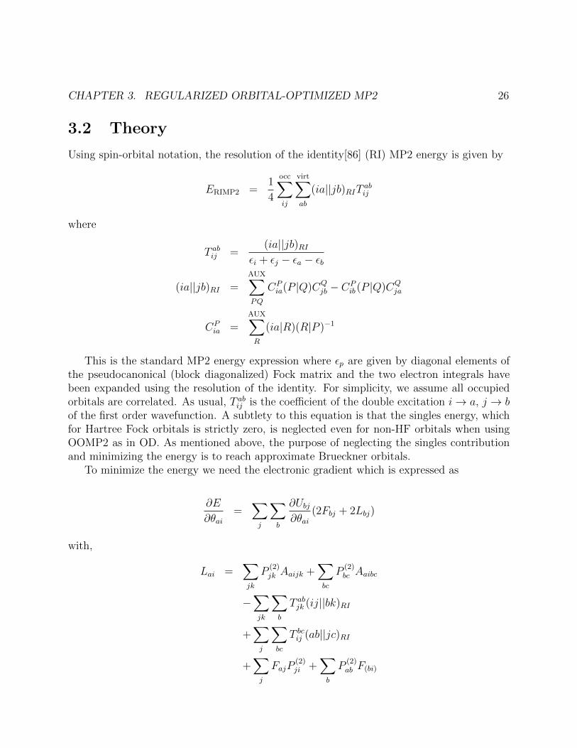
Using spin-orbital notation, the resolution of the identity[86] (RI) MP2 energy is given by
ERIMP2 =1
4
occ∑ij
virt∑ab
(ia||jb)RIT abij
where
T abij =(ia||jb)RI
εi + εj − εa − εb
(ia||jb)RI =AUX∑PQ
CPia(P |Q)CQ
jb − CPib (P |Q)CQ
ja
CPia =
AUX∑R
(ia|R)(R|P )−1
This is the standard MP2 energy expression where εp are given by diagonal elements ofthe pseudocanonical (block diagonalized) Fock matrix and the two electron integrals havebeen expanded using the resolution of the identity. For simplicity, we assume all occupiedorbitals are correlated. As usual, T abij is the coefficient of the double excitation i→ a, j → bof the first order wavefunction. A subtlety to this equation is that the singles energy, whichfor Hartree Fock orbitals is strictly zero, is neglected even for non-HF orbitals when usingOOMP2 as in OD. As mentioned above, the purpose of neglecting the singles contributionand minimizing the energy is to reach approximate Brueckner orbitals.
To minimize the energy we need the electronic gradient which is expressed as
∂E
∂θai=
∑j
∑b
∂Ubj∂θai
(2Fbj + 2Lbj)
with,
Lai =∑jk
P(2)jk Aaijk +
∑bc
P(2)bc Aaibc
−∑jk
∑b
T abjk (ij||bk)RI
+∑j
∑bc
T bcij (ab||jc)RI
+∑j
FajP(2)ji +
∑b
P(2)ab F(bi)

CHAPTER 3. REGULARIZED ORBITAL-OPTIMIZED MP2 27
and,
P(2)ij =
−1
2
∑k
∑ab
T abik Tabjk
P(2)ab =
1
2
∑ij
∑c
T acij Tbcij
Apqrs = (pq||rs) + (pq||sr)= 2(pq|rs)− (pr|ps)− (ps|qr)
Standard notation is used, where Fpq are Fock matrix elements, P(2)pq are elements of the
correction to the two particle density matrix, and Apqrs is from the HF orbital Hessian. Notethat the last two terms of the Lagrangian (Lai) come from off-diagonal Fock matrix elementsand appear since we are not using HF orbitals.
Our proposal is to tame the divergence of the OOMP2 energy by modifying the T am-plitudes which contain the energy denominators. The simplest place to start is to add alevel shift to the zeroth order energies which takes the form of a small constant factor tothe denominator, thus setting a lower limit to the divergence. Our new amplitudes are thusexpressed,
T abij (δ) =(ia||jb)RI
εi + εj − εa − εb − δ
This choice gives the added benefit of leaving the gradient equations unchanged exceptfor the replacement of T with T (δ).
The level shift can be theoretically justified as a repartitioning of the zeroth order Hamil-tonian as,
Hδ0 = H0 + δ · 1
Vδ = V − δ · 1
which leaves the first order energy unchanged, but modifies the first order amplitudes asT abij (δ).
Another way to derive δ-OOMP2 is to start from the Hylleraas functional[87] and penalizelarge amplitudes by including a third term:
JH(T) = 2T†V −T†(H0 − E0)T + δ ·T†T
From here we minimize JH by differentiating with respect to T and setting equal to zero:
∂JH∂T
= 2V + 2(E0 + δ −H0)T = 0

CHAPTER 3. REGULARIZED ORBITAL-OPTIMIZED MP2 28
and we get,
T =V
(E0 + δ −H0)
Thus we arrive at at the same equations by viewing δ as a level shift from repartitioningthe Hamiltonian, or as a quadratic penalty function applied to the T amplitudes. Morecomplicated (i.e. more non-linear) penalty functions are also possible[88].
3.3 Results and Discussion
Divergence
While the possibility of the OOMP2 energy diverging is clear, what is unclear is underwhat circumstances these divergences will interfere with the optimization procedure. Weare limited in our understanding of the energy as a function of orbitals due to the highdimensionality of the problem. One exception, however, is the case of H2 in a minimal basis(in an unrestricted framework), for which the only degrees of freedom to which the energy isnot invariant are the 2 rotations between occupied and virtual alpha and beta orbitals. Thus,for a given bond length, we can plot the OOMP2 energy landscape in three dimensions.
Figures 3.2 and 3.3 plot the energy surface at equilibrium and stretched geometries as afunction of Given’s rotations between occupied and virtual orbitals in α and β subspaces.There are a few points of note to help orient oneself in these plots. First, the (0◦, 0◦) pointcorresponds to the orbitals obtained by diagonalizing the core Hamiltonian and, for minimalbasis H2, corresponds quite nearly to RHF orbitals. Second, since the two axes correspond tomixing α and β orbitals independently, all points that lie off the central diagonal (θα = θβ)will correspond to spin contaminated (unrestricted) orbitals. The final point to note is thatrotation by 180◦ corresponds to multiplying the molecular orbital by -1 and leaves the energyunchanged. Thus the plotted region contains points corresponding to the same orbitals, butwe leave this degeneracy in the plot to get a clearer visual representation of the surface.
When we look at the energy surface at equilibrium, there appears to be a clear, singleminimum corresponding to the RHF solution at the origin. Although some “dents” appearnear the top of the curve, we can safely say that they will have no effect on any optimizationprocedure since they appear near the top of a nearly 1000 kcal/mol high maximum. We canfeel relatively sure that optimization on this energy surface will yield the global minimumsolution without much difficulty.
Once we stretch the bond to 4.0 A, we get a qualitatively different picture. Now, the newunrestricted solution shows up as a wide minimum around the point (140◦, 40◦). Unlike theequilibrium case, there are points on the orbital surface where the energy diverges due to thecoalescence of the HOMO and LUMO energies. In fact, the restricted solution is surroundedby these divergences.

CHAPTER 3. REGULARIZED ORBITAL-OPTIMIZED MP2 29
Figure 3.2: Dependence of the OOMP2 energy (the standard RIMP2 energy without singlescontribution) on the two occupied-virtual mixing angles for the hydrogen molecule in theSTO-3G basis at 0.74 A. The region around the RHF minimum at (0◦, 0◦) is well behaved.
Figure 3.3: Dependence of the OOMP2 energy on the two occupied-virtual mixing angles forthe hydrogen molecule in the STO-3G basis at 4.0 A. Divergences appear for orbitals withunfavorable HF energies but very large negative MP2 energy due to HOMO-LUMO energycoalescence. There is a stable minimum near the UHF solution around (140◦, 40◦), but it isnot the global minimum due to the divergences.
To get a sense of the size of the regularization parameter needed to be to remove thesepits, Figure 3.4 plots the energy surface for δ-OOMP2 for δ values of 100 and 400 mEh. Itshows that in our toy case, one must go to values over 10 eV to tame the divergences ofOOMP2. A value this high will certainly have a significant effect on absolute energies, butpotentially less so on relative energies as we will see. In this case, the unrestricted solutionhas been restored as the global minimum and the divergences have nearly been reducedto saddle points. In general, we expect that level shifts of this magnitude should removedivergences as absolute minima, since there will be a large penalty from the first orderenergy for bringing the HOMO and LUMO orbital energies to degeneracy. Unfortunately,there may still be artificial, shallow local minima, but they will be easily identifiable by aHOMO-LUMO gap of zero.
The difficulty of looking at divergences that arise in OOMP2 is that it is a problem that

CHAPTER 3. REGULARIZED ORBITAL-OPTIMIZED MP2 30
Figure 3.4: δ-OOMP2 orbital energy surface with level shifts, δ, of 100 mEh (left) and 400mEh (right) for the hydrogen molecule in the STO-3G basis at 4.0 A. The level shift of 400mEh has restored the solution near the UHF orbitals to be the global minimum and hasremoved the divergences.
depends on the specifics of the optimization algorithm and can be fixed by knowing theright answer ahead of time (since presumably the final set of orbitals should have a non-zeroHOMO-LUMO gap). Rather than immediately fixing our parameter by how “regularized”it makes the optimization, we choose to look at the problem from a different perspective, byviewing δ as a semi-empirical parameter and testing how it can improve systematic errors inOOMP2. We can then assess how compatible (or incompatible) the two perspectives are.
Test Sets
We proceed by investigating the effect of the δ parameter on errors in calculated atomizationenergies compared to QCISD(T) [89] for the 148 small molecules of the G2 test set [90, 91] inthe cc-pVTZ basis. The G2 test set is chosen as a fair testing grounds since thermochemistryof closed shell systems is definitely not the target of OOMP2; in fact, for such systems,standard RIMP2 will likely be faster and more accurate. In this sense, we hope to parametrizeδ-OOMP2 for general improvement, rather than fit it to a specific problem. The moderatelysized cc-pVTZ basis is used in both reference and OOMP2 calculations with the matchingauxiliary basis set for the resolution of the identity. In this way, we are not compensatingfor basis set incompleteness.
Figure 3.5 shows the root mean square error (RMSE) for δ-OOMP2 as well as the cor-responding δ-RIMP2 and an RIMP2 and OOMP2 variant with directly scaled correlationenergy (as has been previously applied to MP2 [92, 93]). The other two methods are brieflyconsidered here as a way to provide a fair comparison: inclusion of a semi-empirical param-eter will necessarily improve the statistical errors and we want to make sure that the pa-rameterization we are working with gives comparable improvements to other simple, singly-parameterized variants of MP2. These results show that a significantly large regularization
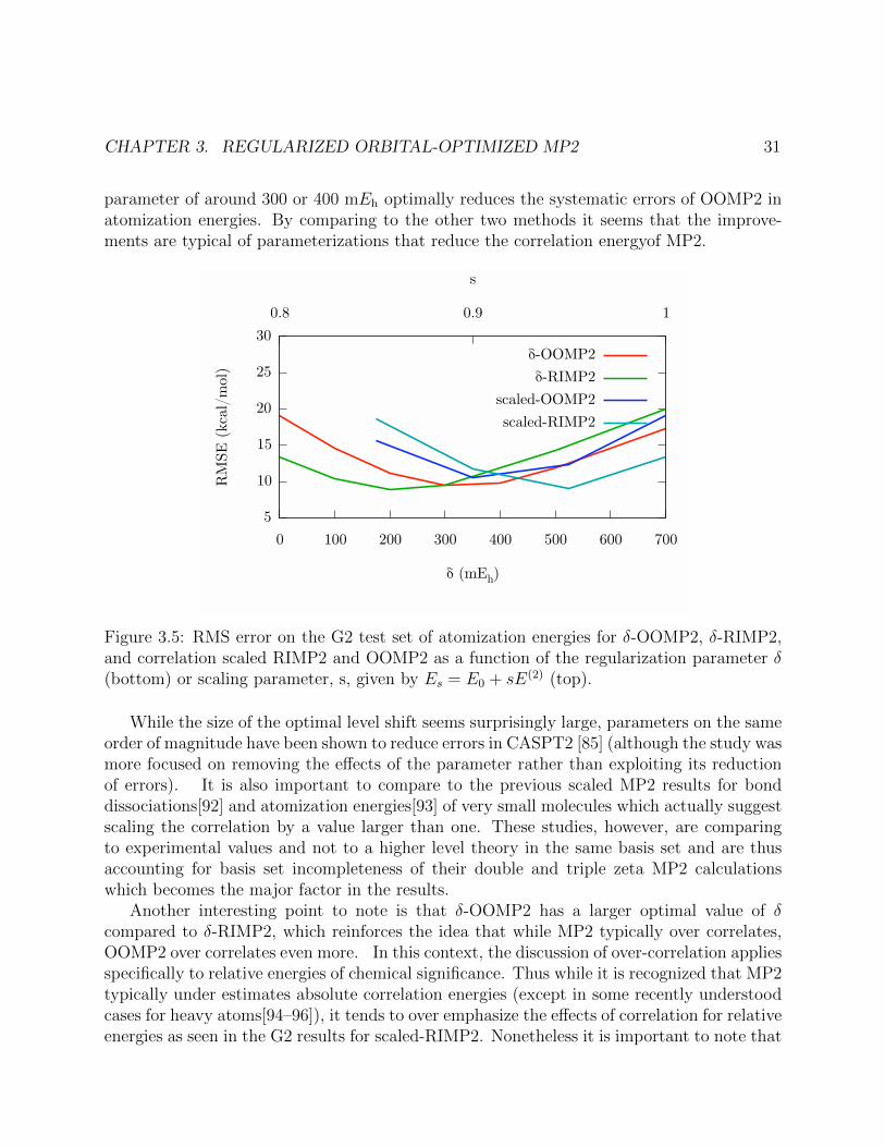
CHAPTER 3. REGULARIZED ORBITAL-OPTIMIZED MP2 31
parameter of around 300 or 400 mEh optimally reduces the systematic errors of OOMP2 inatomization energies. By comparing to the other two methods it seems that the improve-ments are typical of parameterizations that reduce the correlation energyof MP2.
Figure 3.5: RMS error on the G2 test set of atomization energies for δ-OOMP2, δ-RIMP2,and correlation scaled RIMP2 and OOMP2 as a function of the regularization parameter δ(bottom) or scaling parameter, s, given by Es = E0 + sE(2) (top).
While the size of the optimal level shift seems surprisingly large, parameters on the sameorder of magnitude have been shown to reduce errors in CASPT2 [85] (although the study wasmore focused on removing the effects of the parameter rather than exploiting its reductionof errors). It is also important to compare to the previous scaled MP2 results for bonddissociations[92] and atomization energies[93] of very small molecules which actually suggestscaling the correlation by a value larger than one. These studies, however, are comparingto experimental values and not to a higher level theory in the same basis set and are thusaccounting for basis set incompleteness of their double and triple zeta MP2 calculationswhich becomes the major factor in the results.
Another interesting point to note is that δ-OOMP2 has a larger optimal value of δcompared to δ-RIMP2, which reinforces the idea that while MP2 typically over correlates,OOMP2 over correlates even more. In this context, the discussion of over-correlation appliesspecifically to relative energies of chemical significance. Thus while it is recognized that MP2typically under estimates absolute correlation energies (except in some recently understoodcases for heavy atoms[94–96]), it tends to over emphasize the effects of correlation for relativeenergies as seen in the G2 results for scaled-RIMP2. Nonetheless it is important to note that

CHAPTER 3. REGULARIZED ORBITAL-OPTIMIZED MP2 32
this over-correlation is not a universal rule but is a significant trend seen quite clearly inthe 148 molecules of the G2 test set. Finally it is also encouraging that the optimal valueseems quite compatible with the values inferred as suitable for regularization in the previoussection.
Performance of δ-OOMP2 on test sets that typically give standard MP2 trouble are shownin Fig 3.6. In addition to the G2 atomization energies, we have considered the S22 (weakinteractions), RSE43 (radical stabilization energies), and BH76 (barrier heights) test setsfrom Grimme’s GMTKN30 database[97] as well as a subset of the SRMBE12 that excludessecond row transition metals. Calculations on the S22 test set are run in basis sets matchingthe original CCSD(T) values[98] without extrapolation while RSE43, BH76, and SRMB9are run using a T-Q basis set extrapolation[99] to compare to reference values. Since errorsin the various test sets can be orders of magnitude different, all RMS errors are plottedrelative to that of RIMP2 using unrestricted orbitals that have been confirmed as localminima by running a stability analysis. In all cases the regularization parameter improvesthe performance with a degree of insensitivity to the parameter that is surprising but verypromising.
While the S22 test set is not one particularly suited to orbital optimization, it is a sensitiveand important case with systematic errors that, while not improved directly with orbitaloptimization, are reduced by scaling back the correlation energy. These improvements areseen across all subsets of interactions—hydrogen bonding, dispersion, and mixed–but mostprominently improve the dispersion interactions.
Radical stabilization is where OOMP2 really shines and it is good to see that the levelshift reduces error in these systems as well. It is important to recognize that the major failingof RIMP2 in these cases is due to the spin contamination in the reference, and RIMP2 canbe improved using ROHF orbitals which are, however, not local minima in the full orbitalspace of spin polarized orbitals (and hence curves that smoothly separate bonds to correctfragments cannot be obtained).
Barrier heights are another case that requires balancing the description of two differenttypes of systems, in this case ground and transition states. Here too, the largest errors comefrom cases where spin symmetry breaking is not present equally on either side of the reactionleading to cases with large errors; however, these systems can not be simply rescued by arestricting the reference as reducing the degrees of freedom leads to even worse errors.
The significant improvement seen in the description of single reference metal containingcompounds is very encouraging. These systems are better described by the orbital-optimizedreference, but also show great improvement with respect to the level shift.
Frequencies
Recent results[100] have shown that for a collection of small radicals, while standard MP2fails dramatically for vibrational frequencies that involve symmetry breaking, OOMP2 sys-tematically overestimates bond lengths and under estimates frequencies. This overestimation

CHAPTER 3. REGULARIZED ORBITAL-OPTIMIZED MP2 33
Figure 3.6: RMS errors of δ-OOMP2 relative to standard RIMP2 on various test sets. With-out regularization OOMP2 performs worse than RIMP2 for the G2 and S22 test sets but alevel shift of 400 mEh improves δ-OOMP2 over RIMP2 and unregularized OOMP2 for alltest sets.
-0.02
-0.01
0
0.01
0.02
0.03
0.04
0.05
OOMP2
δ-OOMP2
MP2
LiO2 C3+ NO2
HOOH+
cisHOOH+
cisHOOH+
transHOOH+
trans
Bond Length Errors
Err
or v
s. C
CSD
(T)
(Å)
500
1000
1500
2000
2500
500 1000 1500 2000
δ-OOMP2
OOMP2
MP2
Frequency Errors
ω (
cm-1)
ωCCSD(T) (cm-1)
*25006 cm-1*
(a) (b)
Figure 3.7: (a) Bond length errors vs. CCSD(T) of OOMP2, δ-OOMP2, and MP2 forfive small radicals. (b) Harmonic frequencies plotted against CCSD(T) for the same fiveradicals. R2 values for frequencies are 0.979, 0.998, and -0.003 for OOMP2, δ-OOMP2, andMP2 respectively. MP2 and reference CCSD(T) values taken from the work of Bozkaya[100].
of bond lengths fits with our understanding that OOMP2 over correlates: as a single bond ispulled apart from equilibrium, electron correlations tend to grow stronger in the intermediateregime before they die off as the systems become separated. Thus the decrease in correlationenergy from including the level shift parameter should decrease bond lengths, reducing thesystematic errors.

CHAPTER 3. REGULARIZED ORBITAL-OPTIMIZED MP2 34
Figure 3.7(a) shows the results with a 400 mEh level shift parameter confirming theimprovement. The large scale failure of MP2 and systematic improvement of δ-OOMP2 overstandard OOMP2 for frequencies is seen in figure 3.7(b). The improvement is particularlypromising since it shows that the parameter independently chosen based on properties at theexternally fixed geometries of the test sets is transferable to describing the correct equilibriumplacement and local environment on the potential energy surface.
3.4 Conclusion
We have presented a simple proposal for regularizing orbital optimized MP2 for near orbitaldegeneracy. Comparisons to standard OOMP2 and MP2 on various test sets have shown thatchoosing a large nonzero value for δ not only helps the method avoid diverging to artificialminima but also improves the method’s accuracy. We have selected a roughly optimal value of400 mEh to use as the recommended value for δ-OOMP2 based initially on thermochemistry,but which shows improvements for all of the test sets studied in this work. While the costof δ-OOMP2 is the introduction of semi-empiricism, the benefits extend beyond improvedstatistical errors to include the ultimate goal of stabilizing the optimization to the presenceof divergences.
Since one of the greatest drawback of OOMP2 is the computational time required toiteratively calculate the MP2 energy, we plan to apply a level shift to the iterative O(N4)orbital-optimized opposite-spin scaled second-order correlation (O2)[52] to make for a moretractable method. There are also other interesting possibilities for related future work. First,there is great interest in double hybrid density functionals (DHDFs) [101] at present (forinstance [102–105]), including the recent possibility that orbital-optimized DHDFs [106] canoffer significant advantages. Very likely the inclusion of a regularization parameter as acomponent of an OO-DHDF would be useful both for accuracy and stability of the resultingfunctional. Separately, electronic attenuation has been shown to substantially increase theaccuracy of MP2 theory for non-covalent interactions in finite basis sets [107, 108]. It maybe that combining regularization and attenuation will further broaden the applicability ofthese MP2-derived methods.

35
Chapter 4
Stability Analysis without AnalyticalHessians
4.1 Abstract
Wavefunction stability analysis is commonly applied to converged self-consistent field (SCF)solutions to verify whether the electronic energy is a local minimum with respect to secondorder variations in the orbitals. By iterative diagonalization, the procedure calculates thelowest eigenvalue of the stability matrix or electronic hessian. However, analytical expres-sions for the electronic hessian are unavailable for most advanced post-Hartree Fock (HF)wave function methods and even some Kohn-Sham (KS) density functionals. To addresssuch cases, we formulate the hessian-vector product within the iterative diagonalization pro-cedure as a finite difference of the electronic gradient with respect to orbital perturbationsin the direction of the vector. As a model application, following the lowest eigenvalue of theorbital-optimized second order Møller–Plesset perturbation theory (OOMP2) hessian duringH2 dissociation reveals the surprising stability of the spin-restricted solution at all separa-tions, with a second independent unrestricted solution. We show that a single stable solutioncan be recovered by using the regularized OOMP2 method (δ-OOMP2), which contains alevel shift. Internal and external stability analyses are also performed for SCF solutionsof a recently developed range-separated hybrid density functional, ωB97X-V, for which theanalytical hessian is not yet available due to the complexity of its long-range non-local VV10correlation functional.
4.2 Introduction
Self-consistent field (SCF) solutions to wavefunction theory and Kohn-Sham (KS)[109, 110]formalism of density functional theory (DFT) are typically determined by imposing con-straints on the spin orbitals. These constraints not only lower SCF costs, but also allow the

CHAPTER 4. STABILITY ANALYSIS WITHOUT ANALYTICAL HESSIANS 36
approximate wavefunction to share some properties in common with the exact wavefunctionsuch as spin or spatial symmetry. Variational minimization ensures that the energy is sta-tionary with respect to first order changes in the spin orbitals. Therefore, second derivativeswith respect to spin orbital coefficients must be positive for the energy to be a true localminimum, and the procedure to verify this condition is termed stability analysis.
Thouless originally derived the conditions for stability of HF wavefunctions from secondquantization[111]. This was followed by a density matrix-based approach[112], and a refor-mulation of the Thouless conditions to treat both closed and open-shell systems[113, 114].Seeger and Pople[115] devised a systematic approach to treat HF instability beginning withreal spin-restricted HF orbitals, and progressively removing each of these constraints. Foreach case, they obtained the conditions for internal stability, where spin orbitals are variedwithin the space of defined constraints, as well as external stability where one constraint isremoved at a time. Stability analysis for HF involves the calculation of the lowest eigen-value of a stability matrix (or electronic hessian). Since diagonalization of the large stabilitymatrix (whose elements form a fourth rank tensor) may be prohibitive, stability analysis em-ploys iterative diagonalization techniques such as the Davidson method[116]. Fortunately,the critical step in iterative diagonalization, which involves contraction of the stability ma-trix with a trial vector, can be performed in a manner very similar to forming a Fock matrix.Therefore the cost of SCF stability analysis is comparable to SCF costs.
The HF solution is typically used as a reference for advanced methods that incorpo-rate correlation such as second order Møller– Plesset perturbation theory (MP2) and cou-pled cluster (CC) theory, although HF orbitals quite commonly suffer from spatial or spinsymmetry-breaking. To address these problems, orbital-optimized second-order perturba-tion theory (OOMP2)[117] distinguishes itself from standard MP2 by optimizing the zerothorder orbitals in the presence of correlation in an approach based on approximate Brueck-ner orbitals[118]. By optimizing the single reference, artificial spin contamination can beremoved[117–120] and energies as well as properties of open shell molecules can be signifi-cantly improved[117–119, 121–123]. Because the energy is made stationary to changes in theorbitals, a Hellman-Feynman condition applies and all first order properties will be contin-uous as the orbitals change continuously[124]. Recently, δ-OOMP2 has been developed as asimple way to regularize the method against small HOMO-LUMO gaps as well as removingsystematic errors in the method[125]. While approximate forms have been applied in pre-vious studies[119], full analytical expressions for the electronic hessian are unavailable andfinite difference electronic hessians are intractable. As a result, the stability of spin-restrictedand unrestricted formalisms of OOMP2 has not been properly investigated. For the samereason, stability analysis is not available for size-consistent, Brueckner orbital-based coupledcluster techniques such as Brueckner theory doubles (BD)[126] and optimized-orbital cou-pled cluster doubles (OD)[118, 121, 127].

CHAPTER 4. STABILITY ANALYSIS WITHOUT ANALYTICAL HESSIANS 37
The stability conditions for density functionals are essentially analogous to HF, and havebeen derived by Bauernschmitt and Ahlrichs for internal (singlet) and external (triplet)stability of restricted KS-DFT [128]. The formalism, however, requires calculation of sec-ond derivatives of the exchange-correlation energy. Analytical expressions for the secondderivative of the exchange correlation term in KS-DFT are not available for all functionals.ωB97X-V, for instance, is a minimally parameterized range-separated hybrid functional thatcan accurately capture both non-covalent interactions as well as thermochemistry[129]. Thefunctional includes non-local correlation described by VV10[130], for which an analyticalform of the hessian has not yet been derived. In such cases, stability analysis can prove in-tractable since calculation and diagonalization of the full finite difference electronic hessianis not feasible.
Our aim is to establish a technique for stability analysis that is readily applicable to anypost-HF or KS-DFT method, regardless of the availability of analytical second derivativesof electronic energy. We have previously reported a finite differences implementation of theDavidson method to calculate the lowest eigenvalue of a nuclear hessian, which can determinewhether a stationary point calculated using geometry optimization is a minimum or saddlepoint. The same approach can be extended to wavefunction space, where the finite differencesDavidson method is applied to perturbations in the molecular orbitals in order to calculatethe lowest eigenvalue of the electronic hessian[131]. Potential curves for dissociation of H2
are calculated to analyze the stability of SCF solutions for OOMP2 and δ-OOMP2 theory,with some interesting and in some ways remarkable results. Additionally, finite-differencebased stability analysis is applied to the ωB97X-V functional in order to demonstrate theutility of this technique when second derivatives are unavailable.
4.3 Method
The Davidson method is an iterative diagonalization procedure to determine a few extremeeigenvalues of large symmetric matrices when full diagonalization is prohibitive. The al-gorithm is described in detail elsewhere[116, 132]. Briefly, the procedure employs a smallorthonormal subspace of vectors, Bk = [bi] at each iteration k, consisting of dominant com-ponents of the desired eigenvector of a matrix, A. A smaller interaction matrix, BT
k ABk,is constructed and diagonalized to obtain the lowest/highest eigenpair, (λk, yk). The Ritzvector, xk = Bkyk, is then used to estimate the residual error between the exact and approx-imate eigenvector, rk = −(λkI −A)xk. The initial subspace is augmented with a new vectorthat contains this information, and the procedure is iterated until convergence.
The Davidson method was originally applied to large-scale configurational interaction(CI) treatment of wavefunctions[116, 133]. The finite difference implementation of the David-son method can be used when the matrix calculation itself is intractable. For instance, if

CHAPTER 4. STABILITY ANALYSIS WITHOUT ANALYTICAL HESSIANS 38
the matrix A corresponds to the hessian of the energy with respect to nuclear displacements,the exact matrix-vector product, Ab1, is replaced with a finite difference approximation interms of the gradient of the energy (∇E)
Ab1 ≈(∇E(X0 + ξb1)−∇E(X0 − ξb1))
2ξ(4.1)
where b1 is the subspace guess, X0 corresponds to nuclear coordinates of a system, and ξ isthe finite difference step. This expression can be used to calculate a few key eigenvectorsas inputs to mode-following methods for transition state searches on nuclear potential en-ergy surfaces[134–136]. The same principle can also be applied to selective mode trackingin vibrational analysis[137, 138], and characterization of stationary points[131, 139], wherethe lowest one or two eigenvalues of the nuclear hessian are sufficient to verify whether ageometry corresponds to a minimum or transition state, respectively.
Wavefunction stability analysis also requires only the lowest eigenvalue of the electronichessian. Therefore, the finite difference Davidson approach can be extended to stabilityanalysis in cases where analytical hessians are either expensive or unavailable. Since rota-tions between occupied-occupied or virtual-virtual orbitals do not affect the total energy,stability analysis is carried out in the space of occupied-virtual rotations. The most obviouschoice for the initial subspace guess, therefore, corresponds to a HOMO-LUMO rotation. Toavoid possible orthogonality between the guess and the exact eigenvector, a small amount ofrandomness is added in to the subspace guess.
Orbital perturbation in the occupied-virtual space along the subspace guess closely followsthe procedure outlined by Van Voorhis and Head-Gordon[140]. A skew-symmetric unitarytransformation matrix,U1± , is determined by first scaling the guess,
∆1± = ±ξb1 (4.2)
where b1 is the subspace guess corresponding to HOMO-LUMO rotation, ξ(= 0.01) is thefinite difference step, and the number in the subscript corresponds to the iteration. Thetransformation matrix is then given by
U1± = e∆1± (4.3)
The off-diagonal elements of this matrix correspond to rotations in the occupied-virtualspace. The rotated orbitals are given by a unitary transformation of the converged SCForbital coefficients, Cσ
0 , where corresponds to α- or β-spin.
Rotations of α-spin and β-spin orbital coefficients are identical during internal stabilityanalysis of restricted or unrestricted spin orbitals. In order to examine external stability of

CHAPTER 4. STABILITY ANALYSIS WITHOUT ANALYTICAL HESSIANS 39
restricted spin orbitals, on the other hand, spin symmetry needs to be broken. Therefore,α-spin and β-spin orbital coefficients are rotated in opposite directions.
Cβ1+ = −Cα
1+ and Cβ1− = −Cα
1− (4.4)
The hessian-vector product Davidson iterations is then calculated similar to equation 4.1using finite differences of gradients with respect to the rotated coefficients
Ab1 ≈
[(∇E(Cα
1+)−∇E(Cα1−))
2ξ,(∇E(Cβ
1+)−∇E(Cβ1−))
2ξ
]T(4.5)
where A corresponds to the electronic hessian. The Davidson algorithm proposed by Sleijpenand van der Vorst[141] is then employed to iteratively calculate the lowest eigenvalue.
Convergence can be accelerated using a good preconditioner for the residual. In theoriginal Davidson algorithm, the preconditioner at the kth iteration, Ξk, is given by
Ξk = (λkI −D)−1 (4.6)
where D is a matrix consisting of the diagonal elements of A. A reasonable guess for thediagonal hessian is the difference between orbital eigenvalues, ε, in the occupied-virtualspace[140],
Dia,jb = (εa − εi)δijδab (4.7)
where subscripts (i, j) correspond to occupied orbitals and (a, b) to virtual orbitals. In orderto ensure the convergence of the method to the lowest eigenvalue, the preconditioner mustbe negative definite[132]. In cases where preconditioning exceeds a certain cutoff, the cutoffvalue replaces the difference between the eigenvalue and diagonal element. The chosen value,∆E = −0.1Eh, is determined using simple benchmarking of the H2 molecule at equilibriumseparation with B3LYP[142, 143], and correlation-consistent basis sets. The technique isimplemented in a developmental version of Q-Chem 4.2[144], in order to examine internalstability of real restricted or unrestricted orbitals, as well as external stability of restrictedorbitals for OOMP2 theory and any KS-DFT.
4.4 Results
HF vs. orbital-optimized MP2 for bond dissociation
Bond dissociation problems are an important application of stability analysis. The reasonis that many orbital optimization methods will not automatically change the character ofthe orbitals from restricted to unrestricted as the bond is stretched, and therefore stabilityanalysis is needed to detect such a change. Figure 4.1 illustrates the standard result seen for

CHAPTER 4. STABILITY ANALYSIS WITHOUT ANALYTICAL HESSIANS 40
Figure 4.1: Potential curves (green for unrestricted and red for restricted, where it differsfrom unrestricted) for the dissociation of H2 and the associated lowest eigenvalues of thestability matrix (purple for internal stability of the unrestricted solution, blue for externalstability of the restricted solution, where it differs from unrestricted) at the Hartree-Fock(HF) level. The lowest energy solution changes character from restricted to unrestrictedwhen the former becomes unstable.
Hartree-Fock theory for the toy problem of H2 dissociation. The RHF to UHF instabilityis detected by a sign change of the smallest eigenvalue, which occurs at a bond-length ofabout 1.2A. Beyond this distance, the UHF solution exhibits an increasing positive smallesteigenvalue and becomes a distinct, lower energy solution, whilst the smallest eigenvalue ofthe RHF solution becomes steadily more negative.
How does the inclusion of electron correlation in the OOMP2 method affect this picture?The results are shown in Figure 4.2, and at first glance the ROOMP2 and UOOMP2 energycurves look qualitatively similar to the RHF and UHF ones. However the ROOMP2 en-ergy reaches a maximum value around 2.8A and then begins to turn over, as a result of theHOMO-LUMO gap decreasing. The ROOMP2 and UOOMP2 curves actually cross again atstill larger separations than are shown on the figure. What are the implications for orbitalstability analysis? Using the finite difference stability analysis code yields very interestingresults. The ROOMP2 and UOOMP2 solutions are in fact both stable when they are distinct

CHAPTER 4. STABILITY ANALYSIS WITHOUT ANALYTICAL HESSIANS 41
Figure 4.2: Potential curves for the dissociation of H2 and the associated lowest eigenvaluesof the stability matrix using orbital-optimized MP2 (OOMP2) in the cc-pVDZ basis. Theformat follows Figure 6.1. OOMP2 behaves qualitatively differently from HF (see Figure 4.1).The restricted solution is stable (positive eigenvalue) to spin-polarization at all bond-lengths,and a distinct stable unrestricted solution appears at partially stretched bondlengths.
solutions. They apparently do not coalesce upon going to shorter bond-lengths.
As a surprising consequence, despite the Hellman-Feynman condition for OOMP2, thereare still first derivative discontinuities in the dissociation curve for single bond dissociationssuch as H2. It is scarcely visible in Figure 4.2, but this is nonetheless a real effect. As aresult of the ROOMP2 solution always being a true minimum in orbital space, the UOOMP2solution must cross it in the energy coordinate without crossing in orbital space.
To better understand the topography of the solutions we look at the UOOMP2 energyfor H2 as a function of spin-polarization from the ROOMP2 solution in the minimal basiscase where there is only a single orbital rotation angle (θα and θβ) in each of the α and βspaces. A spin polarization angle, φ, can therefore be defined such that θα = φ and θβ = −φ.Figure 4.3 shows the OOMP2 energy as a function of φ for a number of bond lengths closeto the crossing, from ROOMP2 being lowest energy to UOOMP2 being lowest. The keyobservation from Figure 6.3 is the appearance of a second minimum at non-zero φ as the

CHAPTER 4. STABILITY ANALYSIS WITHOUT ANALYTICAL HESSIANS 42
Figure 4.3: The dependence of the OOMP2 energy of H2 in a minimal basis on the spinpolarization angle (see text for definition) at a series of bond-lengths around the criticalvalue at which the character of the lowest energy solution changes. There are two localminima, one restricted and one unrestricted, at these bond-lengths, and at the critical bond-length the nature of the lowest energy solution switches discontinuously.
bond is stretched, whilst the first stationary point (φ = 0) remains a minimum. As thebond-length increases, the second solution eventually becomes the global minimum leadingto the discontinuous change in orbitals as we follow the lowest energy orbitals.
While there is no reason to assume that the global minimum of a nonlinear problem willnot jump between multiple minima as parameters change, it is still surprising to see it heredue to our experience with HF (as exemplified by Figure 4.1). HF is a diagonalization-basedapproach, and so two states with the same energy that can couple through the Hamiltonianshould split in energy. OOMP2 on the other hand adds a perturbative correction, whichin this case preferentially stabilizes the restricted solution and lowers its energy relative tothe unrestricted orbitals bringing their energies to coalescence. Similar observations havebeen made in the context of orbital optimization in active space methods[145, 146]. In casessuch as these, as a consequence of the discontinuous change in orbitals, the potential energysurface exhibits a first derivative discontinuity at the point of the jump in orbital solutions(here, the ROOMP2 to UOOMP2 transition).

CHAPTER 4. STABILITY ANALYSIS WITHOUT ANALYTICAL HESSIANS 43
Figure 4.4: Potential curves for the dissociation of H2 and the associated lowest eigenvaluesof the stability matrix using regularized orbital optimized MP2 (δ-OOMP2) in the cc-pVDZbasis. The format follows Figure 6.1. δ-OOMP2 behaves qualitatively differently fromOOMP2 (see Figure 4.2), but is similar to HF (see Figure 4.1). The restricted solutionbecomes unstable at a critical bond-length, beyond which the unrestricted solution is lowestin energy.
How might one overcome this unphysical behavior of OOMP2, and recover smoother po-tential energy surfaces? We cannot give a complete answer here, but we can apply stabilityanalysis to a modified form of OOMP2 that includes a fixed level shift of 0.4 a.u., termedδ-OOMP2. δ-OOMP2 has been shown to yield systematic improvements relative to OOMP2across a broad range of properties while being robust to divergences during orbital optimiza-tion[125]. The performance of δ-OOMP2 for the dissociation of H2 is shown in Figure 4.4,and presents a striking contrast with OOMP2 shown in Figure 4.2. δ-OOMP2 shows onlyone stable solution at any geometry, like HF, and unlike OOMP2. As a consequence, asshown in Figure 4.5 for minimal basis H2, the optimized orbitals for the global minimumdo not change discontinuously as the bond is stretched, and thus the potential energy sur-face is continuous through first derivatives. Further calculations on a much larger range ofmolecules are required to test the generality of the present positive result, and the stabilityanalysis method introduced here is a crucial tool for this purpose.

CHAPTER 4. STABILITY ANALYSIS WITHOUT ANALYTICAL HESSIANS 44
Figure 4.5: The dependence of the δ-OOMP2 energy of H2 in a minimal basis on the spinpolarization angle (see text for definition) at a series of bond-lengths around the critical valueat which the character of the lowest energy solution changes. For any given bond-length thereis only one local minimum, which changes character from restricted to unrestricted at thecritical bond-length.
4.5 Conclusions
Stability analysis has thus far been limited to formalisms for which analytical second deriva-tives are available since the cost of full finite difference hessian calculation is prohibitive. Wedescribe a hessian-free approach in which the hessian-vector product required for iterativediagonalization within the Davidson method is approximated by finite differences of the gra-dients with respect to rotation of molecular orbital coefficients in the occupied-virtual space.The procedure is implemented for both orbital-optimized post-HF methods such as OOMP2as well as DFT, and can successfully examine internal and external stability with respectto spin symmetry constraints. In future, the implementation will also include internal andexternal stability analysis for complex as well as general spin orbitals. The technique willalso be made available for other orbital-optimized methods such as coupled cluster-basedBD and OD, for which stability analysis has hitherto not been performed.

CHAPTER 4. STABILITY ANALYSIS WITHOUT ANALYTICAL HESSIANS 45
4.6 Acknowledgements
The development of the stability approach is done by the first author of this paper fromwhich this chapter is cut from, Shaama Mallikarjun Sharada. This research was supportedby a grant from Chevron Energy Technology Co., by the Department of Energy Office ofScience Graduate Fellowship Program (DOE SCGF), made possible in part by the AmericanRecovery and Reinvestment Act of 2009, administered by ORISE-ORAU under contract no.DE-AC05- 06OR23100, and by the Office of Science, Office of Basic Energy Sciences, ofthe (U.S.) Department of Energy under Contract No. DE-AC02-05CH11231. We are alsograteful to Narbe Mardirossian for providing instructive examples for the stability analysiswith the ωB97X-V functional, and Dr. Julien Panetier for electrocatalyst geometries. Weacknowledge computational resources obtained under National Science Foundation (NSF)Award No. CHE-1048789 and NSF CHE-0840505.

46
Chapter 5
Exponential Regularized OOMP2 forDissociations
5.1 Introduction
Dissociation processes are good test cases for highlighting the problems associated with thesymmetry dilemma[28]. For example, for Li2 dissociation, restricted MP2 gives a good de-scription of the equilibrium geometry but qualitatively fails in the dissociation limit, whileunrestricted MP2 can handle the dissociation limit properly but fails in the equilibriumregime. In our previous work, we have proposed orbital-optimized second-order perturba-tion theory (OOMP2) as a black box approach that connects the closed shell equilibriumdescription to the unrestricted dissociated state[52, 147].
The OOMP2 method, which can be thought of as a approximation to Brueckner or-bitals[59], optimizes orbitals in the presence of correlation thereby reducing errors from spincontamination and improving descriptions of bond lengths, frequencies, and relative ener-gies[52, 56, 57, 63, 64]. Another benefit of the method is that due to a Hellmann-Feynmanncondition, first derivatives of the energy will be continuous as the orbitals change continu-ously[65]. The possibility of degeneracies leading to failures during optimization encouragedthe development of δ-OOMP2, where a 400 Eh level-shift is added to the T amplitudes toregularize the method[147]. It was shown that this parameterization improved properties ofthe method while also stabilizing the orbital potential energy surface for H2.
Previously, the development of a gradient-based stability analysis algorithm allowed usto calculate the stability of the OOMP2 solutions across dissociation curves and found thesurprising result that for the dissociation of H2, while the energy was changing continuouslyfrom the restricted to unrestricted solution, the wavefunction was not[15]! The restrictedsolution remained stable throughout the curve meaning that instead of the unrestrictedsolution breaking off at the unrestriction point, it formed at a higher energy and the twocrossed in energy but not wavefunction space. It was shown that the δ-OOMP2 is capable
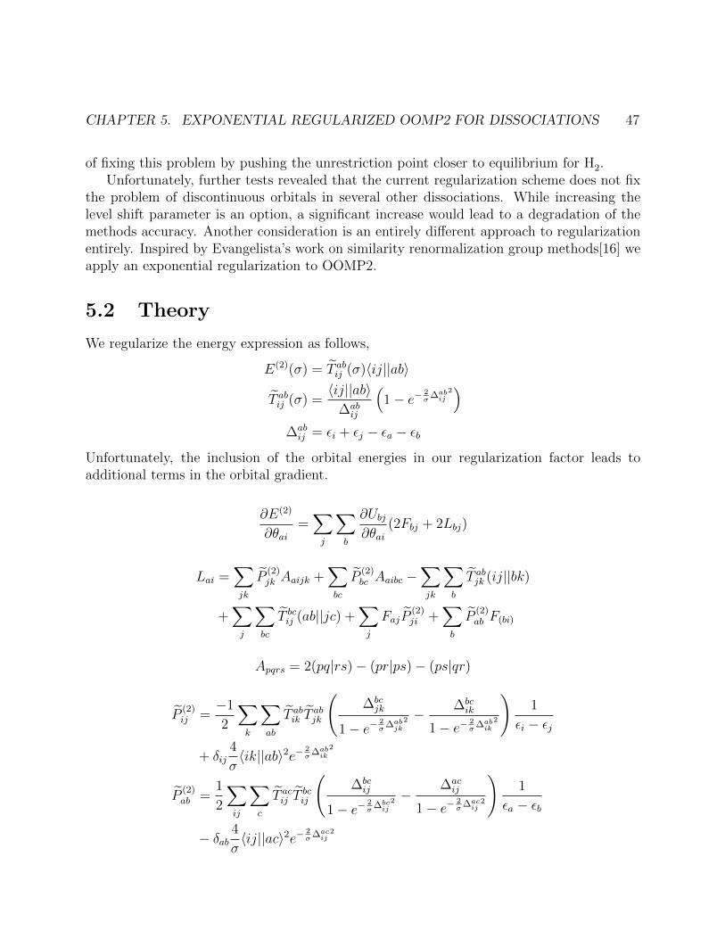
CHAPTER 5. EXPONENTIAL REGULARIZED OOMP2 FOR DISSOCIATIONS 47
of fixing this problem by pushing the unrestriction point closer to equilibrium for H2.Unfortunately, further tests revealed that the current regularization scheme does not fix
the problem of discontinuous orbitals in several other dissociations. While increasing thelevel shift parameter is an option, a significant increase would lead to a degradation of themethods accuracy. Another consideration is an entirely different approach to regularizationentirely. Inspired by Evangelista’s work on similarity renormalization group methods[16] weapply an exponential regularization to OOMP2.
5.2 Theory
We regularize the energy expression as follows,
E(2)(σ) = T abij (σ)〈ij||ab〉
T abij (σ) =〈ij||ab〉
∆abij
(1− e−
2σ
∆abij
2)
∆abij = εi + εj − εa − εb
Unfortunately, the inclusion of the orbital energies in our regularization factor leads toadditional terms in the orbital gradient.
∂E(2)
∂θai=∑j
∑b
∂Ubj∂θai
(2Fbj + 2Lbj)
Lai =∑jk
P(2)jk Aaijk +
∑bc
P(2)bc Aaibc −
∑jk
∑b
T abjk (ij||bk)
+∑j
∑bc
T bcij (ab||jc) +∑j
FajP(2)ji +
∑b
P(2)ab F(bi)
Apqrs = 2(pq|rs)− (pr|ps)− (ps|qr)
P(2)ij =
−1
2
∑k
∑ab
T abik Tabjk
(∆bcjk
1− e−2σ
∆abjk
2 −∆bcik
1− e− 2σ
∆abik
2
)1
εi − εj
+ δij4
σ〈ik||ab〉2e−
2σ
∆abik
2
P(2)ab =
1
2
∑ij
∑c
T acij Tbcij
(∆bcij
1− e−2σ
∆bcij
2 −∆acij
1− e−2σ
∆acij
2
)1
εa − εb
− δab4
σ〈ij||ac〉2e−
2σ
∆acij
2

CHAPTER 5. EXPONENTIAL REGULARIZED OOMP2 FOR DISSOCIATIONS 48
5.3 Results
We first look at the breakdown of δ-OOMP2 for dissociating single and double bonds. Fig 5.1and 5.2 show that for ethane and ethene, δ-OOMP2 jumps discontinuously between orbitals.This discontinuity in the wavefunction is seen in the jump in 〈S2〉 at the unrestriction pointand more definitively through the stability of the restricted solution as seen in the plottedlowest eigenvalue of the orbital Hessian. For ethane, the jump is small; the restricted solutionremains stable for less than 0.1 A after the unrestricted solution becomes the global minima.For ethene, we can see that the restricted solution remains stable throughout the entiredissociation process.
Figure 5.1: Dissociation curve of ethane in an aug-cc-pVTZ basis. 〈S2〉 of the unrestrictedsolution and lowest Hessian eigenvalue for the restricted solutions plotted to show disconti-nuity in orbitals.
To get an idea of how the new exponential regularization effects general performance, welook to the W4-11 small molecule test set of atomization energies, reaction energies, heavyatom transfers, and isomerizations[148]. We see in Table 5.1 that errors are minimized by avalue of σ about 3.2. Looking at the multireference (MR) and nonMR subsets (based on a%TAEe[T4 + T5] diagnostic with a cutoff at ≥ 0.5%) we see that the new parameterizationout performs δ-OOMP2 on non-MR but is poorer for the MR subset. This is promisingas the method is fundamentally single reference and should thus be focused on non-MRproblems. On the other hand, we don’t want to disregard the MR subset as some portion ofthe %TAEe[T4 + T5] diagnostic may be indicative of the single reference, poor zeroth order

CHAPTER 5. EXPONENTIAL REGULARIZED OOMP2 FOR DISSOCIATIONS 49
Figure 5.2: Dissociation curve of ethene in an aug-cc-pVTZ basis. 〈S2〉 of the unrestrictedsolution and lowest Hessian eigenvalue for the restricted solutions plotted to show disconti-nuity in orbitals.
systems OOMP2 is intended to handle. Thus a value of 3.2 appears to be a reasonablecompromise between the error on the subsets and a preference for a higher regularizationparameter.
reg nonMR MR Totalσ-OOMP2 0 7.85 10.63 9.76
2.4 7.11 6.15 6.493.2 6.93 7.01 6.984.0 6.60 8.57 8.14
δ-OOMP2 7.84 5.44 6.37
Table 5.1: Root mean square error (RMSE) in kcal/mol for σ-OOMP2 with various valuesof σ and δ-OOMP2 with the recommended parameterization of 400 mEh.
We now consider our new σ-OOMP2 approach on the highly problematic dissociation ofnon-trivial bonds. Across the board, we see the σ regularization fix the qualitative failing ofuntampered OOMP2. Figures 5.3 and 5.4 show that double and single bonds are dissociatedfrom a restricted equilibrium to the correct asymptotic limit. The clearest way to see thatthe orbitals unrestricted continuously, is that the lowest eigenvalue of the restricted solutioncrosses zero at the same point that the 〈S2〉 value becomes non-zero. This regularization

CHAPTER 5. EXPONENTIAL REGULARIZED OOMP2 FOR DISSOCIATIONS 50
parameter is even capable of dissociating triple bonds continuously as shown in Figure 5.5for ethyne.
Figure 5.3: Dissociation curve of ethane in an aug-cc-pVTZ basis for σ-OOMP2 with an σvalue of 3.2. 〈S2〉 of the unrestricted solution and lowest Hessian eigenvalue for the restrictedsolutions plotted to show discontinuity in orbitals.
With the the orbitals changing continuously across the potential surface due to the newregularization approach, we have restored the first derivative continuity that makes OOMP2particularly appealing. Unlike MP2, response properties of σ-OOMP2 will be continuous dueto the optimization with respect to orbitals and now the important condition that orbitalschange continuously.
5.4 Conclusion
We have further investigated the unexpected behavior of OOMP2 having discontinuous or-bital changes during bond dissociations. Based on a recommendation from the work ofEvangelista, we have implemented a new regularization approach, σ-OOMP2 that is ca-pable of improving thermochemistry as well as fixing the qualitative failures seen duringdissociations by selecting a regularization parameter σ = 3.2.

CHAPTER 5. EXPONENTIAL REGULARIZED OOMP2 FOR DISSOCIATIONS 51
Figure 5.4: Dissociation curve of ethene in an aug-cc-pVTZ basis for σ-OOMP2 with an σvalue of 3.2. 〈S2〉 of the unrestricted solution and lowest Hessian eigenvalue for the restrictedsolutions plotted to show discontinuity in orbitals.
5.5 Acknowledgements
D. S. is supported in part by the Department of Energy Office of Science Graduate FellowshipProgram (DOE SCGF), made possible in part by the American Recovery and ReinvestmentAct of 2009, administered by ORISE-ORAU under contract no. DE-AC05-06OR23100. Thiswork was also supported by the Office of Science, Office of Basic Energy Sciences, of theU.S. Department of Energy under contract no. DE-AC02-05CH11231. We acknowledgecomputational resources obtained under NSF award CHE-1048789.

CHAPTER 5. EXPONENTIAL REGULARIZED OOMP2 FOR DISSOCIATIONS 52
Figure 5.5: Dissociation curve of ethyne in an aug-cc-pVTZ basis for σ-OOMP2 with an σvalue of 3.2. 〈S2〉 of the unrestricted solution and lowest Hessian eigenvalue for the restrictedsolutions plotted to show discontinuity in orbitals.

53
Chapter 6
Regularized CC2
6.1 Introduction
While mean field Hartree Fock (HF) theory often provides a good foundation for calculatingmolecular energies, it has been well established that one needs to go further and accountfor dynamic correlation in order to get energies with acceptable accuracy. Coupled clus-ter formalism has proven to be a valuable approach to describing dynamic correlation bytruncating the expansion by level of excitation or based on ideas of perturbation theory[6].CC2[9] and Møller Plesset second-order perturbation theory (MP2) can both be viewed asperturbative approximations to full coupled cluster singles and doubles (CCSD). In pertur-bation approaches, the molecular Hamiltonian is broken into a mean-field part, F , that issolved exactly within a given basis and the remaining correlated part, ∆V . In CC2, thedoubles amplitude equations are treated to first order in ∆V where singles amplitudes areconsidered zeroth order and doubles are treated as first order. In MP2, by contrast, theamplitudes themselves are expanded in orders of ∆V and the energy is truncated at secondorder[6].
As approximations to CCSD, MP2 and CC2 share several properties; both methods areintermediate in accuracy between HF and CCSD and scale as O(N5). These methods bothhave efficient resolution of the identity implementations[86, 149] and can have their scalingreduced to O(N4) using a scaled opposite spin approximation[150, 151]. While the scalingof the two methods is equivalent, the typical performance is not, with MP2 being faster inpractice due to CC2 involving an iterative O(N5) step and requiring storage of the doublesamplitudes.
Despite their similarities, the two methods have found favor in differing applications–MP2for ground state energies, and CC2 for excited states. Excited states from linear responsetheory can only reliably be obtained for CC2 as MP2 will have second order poles which areinconsistent with the exact result[9, 152]. Methods such as CIS(D)[153, 154] serve as excitedstate analogs of MP2. On the other hand, the iterative nature and observed systematic

CHAPTER 6. REGULARIZED CC2 54
errors of CC2, as well an increased sensitivity to strong correlation have led to it being seenas non-competitive with MP2 for ground state calculations[151, 155]. It can also correctHilbert space topology by removing the artificial separate minima that may occur for bothrestricted and unrestricted orbitals upon bond stretching[15].
One major weakness of MP2 theory is its strong dependence on good HF reference or-bitals. For HF solutions, MP2 theory only includes doubles corrections which is to say that itcannot correct singles amplitudes (which are associated with orbital rotations) beyond firstorder, the same as HF. By classifying single excitations as a zeroth order effect, CC2 solvesthe singles amplitude equations iteratively and to full order using approximate doubles equa-tions. This extra freedom allows the method to correct for deficiencies in the HF orbitalsbut as mentioned previously, can lead to problems when strong correlations are present[155].
In simple cases such as closed shell organic molecules, the HF reference is qualitativelycorrect enough that MP2 is able to account for the correlation energy on top of the HF ref-erence. However, in the more difficult cases of radicals, inorganics, aromatics, and transitionstates, HF orbitals can be qualitatively incorrect, as often signaled by spin contamination[55,56, 156]. In light of these problematic references, orbital-optimized MP2 (OOMP2)[52, 64]was proposed as a way to introduce correlated reference orbitals. This improvement comesat the cost of OOMP2 becoming an iterative fifth order method. While solving the problemof poor references, OOMP2 created new issues of divergences appearing during optimization.We suggested a simple way to correct these divergences by adding a level-shift to the standardT2 equation leading to δ-OOMP2[147]. This level-shift parameter was chosen to be ratherlarge (400 mEh) so as to make optimization more robust but also, importantly, becauseit removed systematic errors in atomization energies, radical stabilizations and geometries,reaction energies, and barrier heights.
In light of the observed improvement of OOMP2 upon inclusion of a regularization param-eter, one might wonder if CC2 could benefit similarly. Although there are no orbital stabilityreasons for considering a level-shift for CC2 since we don’t need to avoid divergences, weconsider it valuable in and of itself to assess the performance of the parameterization onvarious methods to improve systematic errors.
For CC2, it is better to view the parameterization as coming from a penalty on thenorm of T2 which can be introduced in the Lagrangian; this term will be additive with theorbital energies and end up shifting the denominator in the T2 equations. Thus we can viewthe affect of the parameterization as damping the norm of the T2 operator which may besystematically overestimated similarly to MP2. In mathematical terms, the penalty functionserves to regularize otherwise ill-conditioned equations for the CC2 doubles amplitudes.
In this study, we are interested in the extensibility of this simple parameterization to,not only, ground state CC2 calculations, but also more interestingly to excited states. Reg-ularization can be naturally extended to excited state calculations through linear response,or by damping the R2 operator in the equation of motion (EOM) formulation. If damp-ing T2 amplitudes is a robust approach, then improvements in ground state energies shouldsimilarly improve the transformed hamiltonian of EOM-CC2.

CHAPTER 6. REGULARIZED CC2 55
6.2 Computational Methods
For this work, standard CC2 was implemented in QChem[40] taking advantage of the libten-sor library[40]. We can write out the CC2 Lagrangian with the The modifications to thestandard equations[9] is simply the addition of a constant, δ, to the zeroth order matrixelements in the doubles equations:
〈µ1|H + [H,T2]|0〉 = 0
〈µ2|H + [F + δ,T2]|0〉 = 0
The T2 amplitudes can then be solved as a function of δ as:
tabij =〈abij |e−T1HeT1|0〉
εi − εa + εj − εb + δ
The standard EOM-CC2 equations are similarly recast with a modified energy denomi-nator for the doubles:
rabij =〈abij |e−T1HeT1|ck〉rck
εi − εa + εj − εb + δ + ω
For an implementation-level description of these equations see the supplemental informationof Hohenstein et. al.[157]. All calculations are run with the frozen core approximation.
Ground state benchmarks are similar to those considered for assessing δ-OOMP2[147] andinclude the 148 atomization energies from the G2 test set[90, 91] compared to QCISD(T)[89]values in a cc-pVTZ basis. From Grimme’s GMTKN30 database[97] we have consideredbarrier heights and reaction energies from the BH76 set and radical stabilization energies ofthe RSE43 set in a cc-pVTZ basis. Lastly, we’ve looked at the W4-11 small molecule testset which covers a range of atomization energies, reaction energies, heavy atom transfers,and isomerizations using an aug-cc-pVTZ basis set[148]. This set is split into multi reference(MR) and non-MR subsets based on the %TAEe[T4 + T5] diagnostic from the benchmarkdata where molecules with ≥ 0.5% being classified as MR which corresponds to a naturalbreak in the data and selects approximately 30% of the molecules.
Excited state calculations were benchmarked using the singlet excitation test sets of va-lence states from Thiel et. al.[158, 159] and both valence and Rydberg states from Wiberget. al. [160]. Due to the presence of Rydberg states which are ignored in the Thiel bench-marks, excitations were matched up with benchmark values by recalculating CC2 valuesand matching energies within symmetry representation rather than by the order listed bythe term symbol. Energies were calculated using the TZVP and aug-cc-pVTZ basis sets forthe Thiel set and 6-311G(3+,3+)**[161] for the Wiberg set to compare to the benchmarkresults.

CHAPTER 6. REGULARIZED CC2 56
6.3 Results and Discussion
Figure 6.1 plots the root mean square error (RMSE) of δ-CC2 for various values of δ from0 to 400 mEh relative to the RMSE of RIMP2 on the same test sets. By standardizing toRIMP2, these RMSEs allow for the errors to be considered on the same scale and allows fora quick comparison of CC2 and MP2 performance. Before considering the parameterizationof CC2 it is interesting to note that the standard method performs similarly to RIMP2 forthe more well behaved systems (e.g. the RMS error for RIMP2 and CC2 is 13.44 and 12.72kcal/mol for the G2 test set) but mirrors OOMP2 in its improvement on radicals and moredifficult multireference systems (e.g. the RMS errors for RIMP2, OOMP2, and CC2 are4.25, 1.48, and 2.06 kcal/mol for the RSE43 test set).
Mean field HF has a difficult time describing radicals and often qualitatively fails assignaled by a spin contaminated reference; CC2 allows for a modified reference throughthe iterative inclusion of T1 amplitudes which can be viewed as allowing for a correlatedreference. While CC2 cannot be expected to properly describe MR systems, by allowingfor a modified reference, it can at least improve over MP2 which is stuck in the world ofcompletely uncorrelated orbitals. The one exception to expectations here is the lack ofimprovement for barrier heights (RMS error is 4.47 kcal/mol for CC2 and 4.44 kcal/mol forRIMP2) which tend to be less well behaved and thus more poorly described by the mean-fieldapproximation.
Figure 6.1: δ-CC2 RMSE for various ground state test sets divided by RIMP2 RMSE on thesame sets for various values of δ.

CHAPTER 6. REGULARIZED CC2 57
When we look at the effect of regularization through the varying of δ, we see improvementsfor values of δ somewhere between 100 and 200 mEh or simply very little change. The greatestimprovement is seen for atomization energies with most other properties relatively insensitiveto even large values of the δ parameter. Based on these results we select a regularizationparameter of 150 Eh for ground state δ-CC2.
CC2 has been shown to qualitatively fail for calculating the equilibrium geometry ofozone due to its biradical nature[162]. Unlike MP2 and higher level coupled cluster theory,restricted CC2 predicts a barrierless symmetric dissociation due to an unbalanced descriptionof correlation in the biradicaloid species. Turning to δ-CC2 we can see from Figure 6.2 that aregularization parameter of 150 Eh leads to a properly bound state and increasing it furtherprimarily leads to a constant shift in the surface. The regularization appears to make themethod less sensitive to problematic correlations when electrons are well paired.
Figure 6.2: Ozone symmetric dissociation curve at angle 142.76◦ for CC2 with regularizationparameters 0, 100, 150, and 200 mEh and CCSD in an aug-cc-pVTZ basis.
Excited states for molecules in the Thiel test set are calculated in the TZVP and aug-cc-pVTZ basis sets. Table 6.1 shows an analysis of the errors with respect to the subsetof 22 excitations which were calculated with CC3 as the more approximate CCSDR(3)[163]results have nearly the same systematic error as CC2 with respect to the higher level CC3(mean error 0.08 vs 0.11)[159].
Although the performance on these valence states is not an improvement, the accuracy isonly slightly degraded with the addition of the regularization parameter. To more completelyunderstand the effects of regularization, we also consider the excited state benchmarks of

CHAPTER 6. REGULARIZED CC2 58
TZVP aug-cc-pVTZδ 0 100 200 0 100 150 200
ME 0.14 0.21 0.27 0.11 0.20 0.24 0.27RMSE 0.25 0.31 0.37 0.17 0.25 0.29 0.33MAX 0.86 1.00 1.12 0.43 0.56 0.64 0.72
Table 6.1: Excited state errors on the Thiel test set for regularized δ-EOM-CC2 vs. CC3values in TZVP and aug-cc-pVTZ basis for varying values of δ. All errors in eV.
Wiberg, which contain both valence and excited states. Table 6.2 shows the performance ofδ-EOM-CC2 on the total test set as well as the 39 Rydberg and 30 valence states separately.Here we see that again, the systematic error for valence states is slightly increased, butnow this degradation is compensated by improved performance on Rydberg states. Previousstudies have characterized EOM-CC2 as having difficulties with Rydberg states comparedto other methods[164], so here we can view the regularization as creating a more balanceddescription of two subsets.
Total Rydberg Valenceδ 0 100 150 200 0 100 150 200 0 100 150 200
ME -0.18 -0.4 0.01 0.06 -0.48 -0.34 -0.28 -0.22 0.20 0.35 0.39 0.44RMSE 0.53 0.48 0.46 0.45 0.60 0.45 0.38 0.32 0.42 0.52 0.54 0.57MAX 1.25 1.29 1.31 1.33 1.25 1.04 0.95 0.86 1.00 1.29 1.31 1.33
Table 6.2: Excited state errors on the Wiberg test set for regularized δ-EOM-CC2 values ina 6-311(3+,3+)G** basis for varying values of δ vs. accurate experimental values. All errorsin eV.
6.4 Conclusion
The regularization approach created to avoid divergences in OOMP2 has been extended toCC2 for the dual purpose of creating a method with lower systematic errors at no computa-tional cost and assessing the robustness of this particular semi-emperical parameterization.Benchmarks on ground state systems show improvements that are maximized nearly acrossthe board at around δ = 150 mEh which we suggest for all future work. For excited states,the same regularization parameter is seen to create a more balanced description of Rydbergand valence states. The improved performance of δ-CC2 across a wide range of ground statetest sets shows the efficacy of the simplistic regularized T2 approach to parameterization,while the excited state results show that these same ground state improvements might notalways transfer to all types of excited states but may still create a more robust, balanced

CHAPTER 6. REGULARIZED CC2 59
method, as evidenced by lower overall RMS error in the test sets containing both valencestates (degraded slightly) and Rydberg states (improved significantly).
6.5 Acknowledgements
Many thanks to Evgeny Epifanovsky for his work on the object-oriented ccman2 moduleand his assistance in developing within it. D. S. is supported in part by the Department ofEnergy Office of Science Graduate Fellowship Program (DOE SCGF), made possible in partby the American Recovery and Reinvestment Act of 2009, administered by ORISE-ORAUunder contract no. DE-AC05-06OR23100. This work was also supported by the Office ofScience, Office of Basic Energy Sciences, of the U.S. Department of Energy under contractno. DE-AC02-05CH11231. We acknowledge computational resources obtained under NSFaward CHE-1048789.

60
Chapter 7
Path Integrals for AnharmonicVibrational Energy
7.1 Introduction
An electronic structure theorist’s first approximation is to assume the nuclear and electronicproblems are separable and then focus on the electrons. When accuracy is limited by neglectof nuclear vibrations or if nonzero temperature estimates of thermodynamic quantities arerequired, the vibration problem comes back to the forefront. The obvious starting point whendealing with vibrations is the harmonic approach which simply requires a calculation of thematrix of second derivatives of the electronic energy with respect to nuclear displacements–the Hessian. Diagonalizing the Hessian gives us the frequencies, reduced masses, and normalmodes from which we can calculate harmonic approximations to zero-point vibration energy(ZPE) as well as any other thermodynamic quantities we desire because we have a simpleanalytic form for the partition function for a harmonic oscillator,
QHO =e−
12β~ω
1− e−β~ω
While simple in form and straightforwardly calculated, the harmonic approximation isstill fundamentally limited in accuracy. This limitation can be a foundational one whencomparing to high accuracy experimental results or if dealing with cold, light atoms. To gobeyond this level of electronic structure theorist can turn to several methods which will bevery familiar from experience with electrons, namely VSCF, VPT, and VCI.
Like their electronic counterparts, accuracy comes at a cost. For VCI, reasonable ac-curacy can be obtained by including up to quadruples but doing so scales O(N8), but thepresence of Fermi resonances can lead to catastrophically bad performance. Another is-sue that arises with the wavefunction, based approaches to the vibrational problem is thathigher derivatives with respect to nuclear displacements must be calculated either by havingspecially implemented code or using cumbersome finite difference.

CHAPTER 7. PATH INTEGRALS FOR ANHARMONIC VIBRATIONAL ENERGY 61
Another way to calculate the full vibrational energy is to use a real space path inte-gral approach with Monte Carlo sampling (PIMC). Broadly, the advantages are that themethod can be carried out with only single-point energy evaluations and that the samplingis not inherently superlinearly scaling (although this depends very much on the efficiency ofsampling). The drawback is in the huge prefactor that comes from gathering a statisticallysignificant number of samples, and the fact that comes from gathering a statistically signifi-cant number of samples, and the fact that each sample still costs as much as the single pointevaluations from your model for the electrons.
What we propose then is to take the dearth of information about the system that we’vegained from the Hessian and develop a PIMC method that efficiently samples just the re-maining anharmonic part of the vibrational energy. To do this we apply a static harmonicpropagator (as opposed to the more standard free particle propagator) sampled with Levyflights for large scale, global moves and in conjunction with thermodynamic integration sothat we can estimate anharmonicity directly.
The harmonic oscillator propagator has been used in the past statically for toy sys-tems[165] as well as dynamically in several cases[166, 167]. Various other high level propa-gators have also been proposed[168–170]. We are interested primarily in the static harmonicpropagator as the various others require calculations of the gradient or hessian of V at eachstep as opposed to just a single point value, which would make the method too costly toconsider applying with electronic structure theory.
Thermodynamic integration[171] gives us a direct way to calculate free energy differencesbetween two given Hamiltonians and has been used on a broad class of problems, from re-action profiles[172–176], to isotopic substitution energies[177], to most relatedly anharmoniccorrections for high temperature classical vibrational energy[178].
We were initially interested in high accuracy vibrational energies after a study on sulfate-water clusters found that their assignment of low energy conformers was limited by theaccuracy of their zero-point energy which had significant anharmonicity[179, 180]. Thereare many low energy conformations for 6 water clusters, but their relative energies aredramatically affected by vibrational energies due to differing number of suflate-water andwater-water hydrogen bonds.
7.2 Theory
Model
As a quantum thermodynamics approach, PIMC[13, 181] starts with the partition function,which is the trace of the Boltzmann operator, and then expanding in a position basis, insertsP resolutions of the identity.
Q =∫. . .∫dx1 . . . dxP 〈x1|e−
βPH |x2〉 . . . 〈xP |e−
βPH |x1〉

CHAPTER 7. PATH INTEGRALS FOR ANHARMONIC VIBRATIONAL ENERGY 62
The purpose of inserting the P states is that now we can use high temperature approxima-tions for each of the P density matrix elements. The Trotter approximation allows us tosplit the density matrix elements into two–one whose distribution we know and one which
is diagonal in the position basis, both at an effective temperature ε =β
P.
e−βP
(H0+∆V ) = e−βPH0e−
βP
∆V +O((
βP
)2[Ho,∆V
])Thus if we pick P large enough, we can make the error as small as we want. It is alsoimportant to note that the error in the Trotter approximation can be reduced by reducing[H0,∆V ], most obviously by reducing the magnitude of ∆V .
It’s worth noting that in the context of PIMC the Boltzmann operator is also referredto as the propagator. This interpretation is built on the idea that the Boltzmann operator
can equivalently be viewed as an imaginary time propagator through e−βH = e
iτ
~H
withτ = −iβ~. Thus PIMC can be interpreted as approximating a cyclic path of time iβ~ by Pshort time steps.
The standard, most general approach to PIMC involves taking H0 to be T , the free par-ticle Hamiltonian, which means ∆V becomes the entire V . Since molecules are bound stateswe must have a small step size (large P ) to properly approximate the full propagator. Thebenefits of the free particle propagator (FFP) are simplicity, spatial invariance, and modelinvariance (we don’t need any information about V to from FP density matrix elements).Given that we care about low T vibrational energies for systems where we already havecalculated Hessians, it makes sense to use the system specific information to improve oursampling approach.
After transforming from standard cartesians to normal modes, we now split the Hamil-tonian using the harmonic reference as our short time propagator,
〈xi|e−βPH |xi+1〉 =
(2π~2β
mP
)− 12
γcsch(γ)e− βP
(mω2
2γ(tanh( γ
2)(x2i+x
2i+1)+csch(γ)(xi−xi+1)2)+∆V (xi)
)
Where we use the variable γ =β~ωP
, which should be viewed as the ratio of quantum
vibrational spacing versus thermal fluctuations at our artificially high temperature, ε. Wecan calculate a primitive energy estimator in this representation to get,
εE(x1, . . . , xP ) = 1P
P∑i=1
12~ω coth(γ) + 1
2~ω2
[sech2(γ)x2
i − coth(γ)csch(γ)(xi − xi+2)2]
+∆V (xi)
The important points to know about this estimator are that it provides an estimate ofthe total vibrational energy (we get the anharmonicity by subtracting off the exact harmonic

CHAPTER 7. PATH INTEGRALS FOR ANHARMONIC VIBRATIONAL ENERGY 63
energy) and that, similar to its free particle counterpart, its variance increases with P [182].This increased variance is particularly troublesome since increasing P already grows oursystem size and frustrates sampling and now it also increases the number of samples we needto reduce sampling error! This variance is also the variance in the estimation of the entirevibrational energy which is potentially an order of magnitude larger than the anharmonicenergy, which is all we actually care about calculating.
One way to avoid these problems is to directly sample the anharmonicity using thermo-dynamic integration (TI). TI is a way to calculate free energy differences between two statesgiven a parametrized Hamiltonian, Hλ, that continuously connects them as λ varies from 0to 1.
Hλ = T + (1− λ)V0 + λV1
Fλ = − logQλ
β
F1 − F0 =∫ 1
0dλdFλdλ
=∫ 1
0dλ
∫dqβ(V1 − V0)e−βHλ
βQλ
=∫ 1
0dλ〈V1 − V0〉λ
Where 〈·〉λ denotes the thermodynamic average sampled with Hλ. Its worth noting thatto estimate the anharmonicity we cannot simply sample ∆V using the full H since,
Efull − EHO = 〈εest〉full − 〈εHOest 〉HO6= 〈∆V 〉full
This path from H0 to H1 can be any number of options but ideally we will pick thesmoothest, most linear path to expedite the numerical quadrature. We apply Gaussianquadrature to approximate the integration over λ, which we mention primarily because theinferior trapezoid approximation is still commonly used by some in the field[176]. For ourpurposes, H0 is the harmonic reference and H1 is the full Hamiltonian so we can proposeHλ = H0 + λ∆V . For anharmonicity in clusters we will find this path gives us nearly lineartransitions.
One major issue that must be addressed is that in invoking the local harmonic reference,we lose the spatial invariance of our sampling and our choice of coordinate system becomesvery important. The important factor is to select coordinates in which the potential writtenin normal modes will remain harmonic for as long as possible. While this is a hard problemto solve in general, we have a very good heuristic solution for molecular vibrations in internalcoordinates selected based on chemical bonding[183, 184].
With the goal of using a non-redundant, black-box approach to selecting internal co-ordinates, we apply the delocalized internals of Baker et. al.[185, 186]. We use an atom

CHAPTER 7. PATH INTEGRALS FOR ANHARMONIC VIBRATIONAL ENERGY 64
specific distance criterion to determine bonds (which may need to be modified by the userfor unusual systems) as well as all possible bonds and torisions between bonds; for each sepa-rated cluster, we add in local translations and rotations and given all these primitive internalcoordinates we transform to delocalized, non-redundant internals by doing a singular valuedecomposition on the B matrices.
The last issue to consider when putting together our model is what we will use for thecalculation of electronic energy to give us V . While there is nothing formally stopping usfrom using electronic structure theory, the large number of expected samples discourages usfrom doing so. We propose the use of parameterized force fields to calculate anharmonic cor-rections to higher accuracy harmonic results. Although the absolute energies from forcefieldswill have large errors and even the errors in the harmonic energy tend to be too large, bylooking at the anharmonic corrections, errors are inherently on a smaller order of magnitude.
Sampling
To evaluate the multidimensional integrals of our path integral model, we turn to theMetropolis Monte Carlo algorithm, taking adavantage of our known harmonic informationto improve sampling efficiency. For sampling a value A(x) using the Hamiltonian H we have,
〈A(x)〉H =
∫. . .
∫ ( P∏i
dxi ρ0(xi, xi+1, ε)
)∑i
A(xi)
P
∏i
e−ε∆V (x)
Q
ρ0(xi, xi+1, ε) = 〈xi|eεH0|xi+1〉
To do this efficiently we propose moving a subsection of the P beads at a time using theanalytic distribution from ρ0 and accept or reject them based on weights e−ε∆V , an approachreferred to as Levy flights. Using the known ρHO distribution allows us to dramaticallyimprove our sampling by taking steps correctly based on the harmonic potential and thenaccepting or rejecting based only on ∆V . This is much more efficient compared to the freeparticle approximation which only considers mass and temperature in determining steps andmush accept/reject based on the larger full V . With Levy flights the only parameters leftto adjust our sampling are the number of degrees of freedom we sample at a time and thefraction of beads that we move per step; we choose these values to give us acceptance ratesof near 60-70%.
While we will have to look at test cases to assess model error, sampling error can be

CHAPTER 7. PATH INTEGRALS FOR ANHARMONIC VIBRATIONAL ENERGY 65
much more easily understood. We can estimate the variance in the mean by,
〈(〈∆V 〉 −∆V )2〉 =σ2
N+
2
N2
N∑i<j
(〈∆Vi∆Vj〉 − 〈∆Vi〉〈∆Vj〉)
=σ2
N
(1 +
2
N
N∑k=1
(N−k∑i=1
〈∆Vi∆Vi+k〉 − 〈∆Vi〉〈∆Vi+k〉σ2
))
=σ2
N
(1 + 2
∑k
A(k)N − kN
)
≡ σ2
N2τ
Where ∆V and σ2 are the mean and variance of the estimator over all the samplingpoints. By keeping track of some finite portion of the autocorrelation function, A(k), say1000 points, we can construct the variance in the mean precisely accounting for correlations.The next assumption that the mean value is normally distributed over our sampling pointsis fairly reasonable given the Central Limit Theorem and our the large sample sizes. Thisallows us to calculate a range that we are 95% confident contains the correct mean (for agiven model physics) as,
95% CI = ±1.96σ
√2τ
N
Our implementation estimates the number of samples required to get the confidence inter-val to be within a 5% relative error and sets the run length after running for an initializationperiod.
7.3 Results and Discussion
Model Systems
Before attempting to study water-sulfate clusters we will study some well characterizedmodel systems: a Morse potential model for H2, H2O, and H2O dimer. The methods weconsider are full vibrational energy calculations using free particle propagator (FPP) andHO propagator, as well as TI using the HOP.
Additionally, before we begin looking at systems, we need to determine the temperaturefor our sampling. Often specific temperatures are stipulated by experimental conditions butif ZPE is sought, low finite temperatures must be used as an approximation. A temperatureof 60 K (corresponding to about 0.12 kcal/mol or 34 cm−1 thermal fluctuations) is usedwhich is effectively 0 K on the energy scales we’re considering. PIMC sampling begins to

CHAPTER 7. PATH INTEGRALS FOR ANHARMONIC VIBRATIONAL ENERGY 66
become much more difficult at lower temperatures and begins to require larger values for Pbut it possible. While 60 K is not zero, higher vibrational states are effectively unpopulatedand we will consider energies and free energies at this temperature as ZPE.
The last remaining consideration before applying TI to test systems is that we haven’tdescribed yet is how many points we’ve chosen for our numeric integration of 〈∆V 〉λ. Figure?? shows a plot of 〈∆V 〉λ versus λ for several of our test systems using 11 grid points.As hinted at earlier, the plots for these small molecules are very linear, which mean wecan accurately integrate them with a single quadrature point! It is important to recognizethat all these systems are of clusters of small molecules, notably without bond torsions,so this fortuitous linearity must be reconsidered before applying the TI approach to morecomplicated molecules.
From these test systems, we see that our TI approach allows us to describe low temper-ature vibrations with a dramatically reduced P and N value compared to FPP and HOPapproaches. It also appears that we can achieve nearly zero vibrational error by choosingP = 200 for all theses systems and reduce all errors except electronic error due to our forcefield to small, controlled values within 5% of the anharmonic ZPE we’re calculating.
Figure 7.1: Plot of 〈∆V 〉λ as a function of lambda for sampling with P = 200. R2 values forthe fits are 0.996, 0.984, and 0.998 for the monomer, dimer and sulfate cluster respectively.
From the Morse oscillator we see that sampling using the HOP and TI yields improve-ments on two fronts: the higher level description of the physics leads to a reduction in thenumber of beads, P , required to get the same model error and improvements to samplinglead to a reduction in sampling number, N to get the same statistical errors. Figure 7.2

CHAPTER 7. PATH INTEGRALS FOR ANHARMONIC VIBRATIONAL ENERGY 67
shows the dramatic improvement from using HOP and TI with respect to P ; each methodimproves on the former by a factor of 2.
From Table 7.1 we can see that the number of sampling points needed to get the samelevel of statistical errors increases dramatically with P for FPP, slightly less so for HOP,and much less so for TI. There are a couple important facts to consider when looking at thisTable. First, since these errors are considered relative to the total anharmonic ZPE we needto compare the methods across P values with similarly reduced model error: for H2 we needto compare P values of 400 for FPP to 200 for HOP 100 for TI since these all give similarerrors with respect to P . This comparison shows how each new approach reduced samplingerrors by a full order of magnitude. Second the number of single point calculations requiredis really P times N so higher P values additionally increase the number of sample points(and explains why required N values can decrease with P since NP is still increasing).
Figure 7.2: Errors in anharmonicity on a Morse potential of H2 using the free particle andharmonic propagator full energy approaches as well as thermodynamic integration. TheMorse potential is parameterized with De = 0.176 and a = 1.4886.
Figures 7.3 and 7.4 show results for water monomer and dimer using the standard po-larizable AMOEBA[187–189] force field for water[190, 191]. We see similar multiplicativeimprovement of TI over HOP and HOP over FPP in the monomer case. Unlike the Morsepotential, for which we are comparing to an exact result using the same model potential asour path integrals, for the H2O cases and beyond, we will be using forcefields for our PIMCbut have reference values from electronic structure. This elucidates the three types of errorin our method: statistical (controlled by N), vibrational (controlled by P), and electronic

CHAPTER 7. PATH INTEGRALS FOR ANHARMONIC VIBRATIONAL ENERGY 68
P H2 Water Monomer Water Dimer Sulfate 3H2O Sulfate 6H2OFPP 50 10580 8502
100 24660 81668200 1519848 636924300 11581045 1574675400 26368856 3462925
HOP 50 271278 36574 140365100 427778 124347 222831200 2429968 463723 711451300 5334265 856822 761297
TI 50 158440 17276 17276 31056 25657100 408121 15360 15360 31362 15070200 338591 17107 17107 18349 31702300 275426 11551 11576 19033 31311
Table 7.1: Table of the number of samples required to reduce sampling error to within 5%of calculated anharmonic ZPE.
(inherent in the method used for single point calculations). These errors are also illustratedwell in Figure 7.3; statistical error is in the error bars, vibrational disappears as you reachthe asymptote, and electronic is the difference between the asymptote and zero. Assumedin the previous sentence is that the reference is exact, which for the H2O reference of a fullgrid approach using CCSD(T) results, is probably close enough to being true[192].
Not so clear is the reference value used for the water dimer[193]. Here electronic erroris quite low as the calculations are run with CCSD(T) again, but here the anharmonicityis only accounted for by VPT2. Thus, the difference between the TI P = 200 values andthe reference then are primarily due to the vibrational errors of the reference added to theelectronic error from the PIMC calculation (plus smaller contributions from statistical andvibrational).
Sulfate-Water Clusters
Before we begin calculating enharmonic ZPE for various sulfate clusters we will study thelowest energy 3 H2O cluster further. Figure 7.5 shows that we get similar behavior withrespect to P as in the small test cases. This cluster has also been studied with CC-VSCFwith MP2 electronics and VPT2 and TOSH with B3LYP electronic energies[179, 194] andwe compare to these results in Table 7.2.
While there are deviations between the fairly high level CC-VSCF values and our PIMCresults, these differences are not entirely due to the electronic error in the TI approach. TheCC-VSCF reported values neglect the lowest 14 out of 36 modes. While low modes account
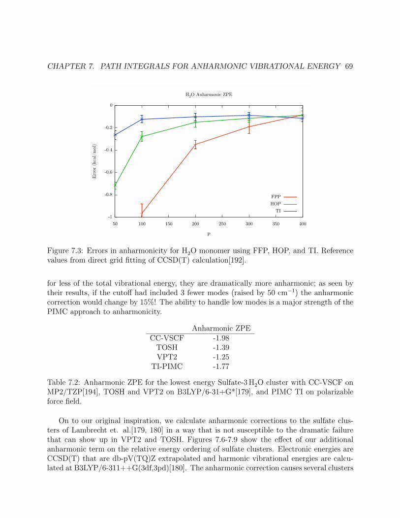
CHAPTER 7. PATH INTEGRALS FOR ANHARMONIC VIBRATIONAL ENERGY 69
Figure 7.3: Errors in anharmonicity for H2O monomer using FFP, HOP, and TI. Referencevalues from direct grid fitting of CCSD(T) calculation[192].
for less of the total vibrational energy, they are dramatically more anharmonic; as seen bytheir results, if the cutoff had included 3 fewer modes (raised by 50 cm−1) the anharmoniccorrection would change by 15%! The ability to handle low modes is a major strength of thePIMC approach to anharmonicity.
Anharmonic ZPECC-VSCF -1.98
TOSH -1.39VPT2 -1.25
TI-PIMC -1.77
Table 7.2: Anharmonic ZPE for the lowest energy Sulfate-3 H2O cluster with CC-VSCF onMP2/TZP[194], TOSH and VPT2 on B3LYP/6-31+G*[179], and PIMC TI on polarizableforce field.
On to our original inspiration, we calculate anharmonic corrections to the sulfate clus-ters of Lambrecht et. al.[179, 180] in a way that is not susceptible to the dramatic failurethat can show up in VPT2 and TOSH. Figures 7.6-7.9 show the effect of our additionalanharmonic term on the relative energy ordering of sulfate clusters. Electronic energies areCCSD(T) that are db-pV(TQ)Z extrapolated and harmonic vibrational energies are calcu-lated at B3LYP/6-311++G(3df,3pd)[180]. The anharmonic correction causes several clusters

CHAPTER 7. PATH INTEGRALS FOR ANHARMONIC VIBRATIONAL ENERGY 70
Figure 7.4: Errors in anharmonicity for H2O dimer using HOP and TI. The reference hereis based on CCSD(T) electronics, but only VPT2 for nuclear energies[193].
to change ordering, including the global minimum of the 5 H2O clusters. The presence oferror bars shows shows the statistical error, which could be further reduced through extrasampling, but it is important to realize that there are additional, non-quantified errors dueto the DFT harmonic calculation as well as the use of forcefields that are likely to be on asimilar scale of 0.1 kcal/mol.
7.4 Conclusion
We have developed a new approach to calculating anharmonic vibrational energy correctionsby combining the idea of using a local harmonic approach with thermodynamic integration,which allows us to systematically reduce vibrational errors for a given electronic model. Themethod can sample difficult, low temperatures by taking advantage of an improved zerothorder propagator, but the cost comes in the form of only applying at temperatures lowenough that the sampled region of phase space is well characterized by the minimum energypotential well. The cost of Monte Carlo sampling is that a large amount of single pointsmust be calculated, but due to improvements in efficiency, we’ve calculated accurate valueswith on the order of 4 × 10⁵ single point calculations for systems of 63 modes. Given fastenough algorithms, the TI approach can be applied to electronic structure single points justas easily as force field calculations to further reduce errors.

CHAPTER 7. PATH INTEGRALS FOR ANHARMONIC VIBRATIONAL ENERGY 71
Figure 7.5: Anharmonic ZPE for Sulfate 3 H2O cluster using TI.
7.5 Acknowledgements
D. S. is supported in part by the Department of Energy Office of Science Graduate FellowshipProgram (DOE SCGF), made possible in part by the American Recovery and ReinvestmentAct of 2009, administered by ORISE-ORAU under contract no. DE-AC05-06OR23100. Thiswork was also supported by the Office of Science, Office of Basic Energy Sciences, of theU.S. Department of Energy under contract no. DE-AC02-05CH11231. We acknowledgecomputational resources obtained under NSF award CHE-1048789.

CHAPTER 7. PATH INTEGRALS FOR ANHARMONIC VIBRATIONAL ENERGY 72
Figure 7.6: Relative Energies of Sulfate 3 H2O clusters using TI.
Figure 7.7: Relative Energies of Sulfate 4 H2O clusters using TI.

CHAPTER 7. PATH INTEGRALS FOR ANHARMONIC VIBRATIONAL ENERGY 73
Figure 7.8: Relative Energies of Sulfate 5 H2O clusters using TI.
Figure 7.9: Relative Energies of Sulfate 6 H2O clusters using TI.

74
References
(1) Boys, S. F. Electronic Wave Functions. I. A General Method of Calculation for theStationary States of Any Molecular System. Proc. R. Soc. A Math. Phys. Eng. Sci.Feb. 1950, 200, 542–554.
(2) Taketa, H.; Huzinaga, S.; O-ohata, K. Gaussian-Expansion Methods for MolecularIntegrals., en J. Phys. Soc. Japan Nov. 1966, 21, 2313–2324.
(3) Gill, P. M. W.; Pople, J. A. The prism algorithm for two-electron integrals. Int. J.Quantum Chem. Dec. 1991, 40, 753–772.
(4) Szabo, A.; Ostlund, N. S., Modern Quantum Chemistry ; Dover Publications: 1996,p 466.
(5) Davidson, E. R. The iterative calculation of a few of the lowest eigenvalues andcorresponding eigenvectors of large real-symmetric matrices. J. Comput. Phys. Jan.1975, 17, 87–94.
(6) Shavitt, I.; Bartlett, R. J., Many-Body Methods in Chemistry and Physics, 1st; Cam-bridge University Press: New York, 2009.
(7) Bartlett, R. J. Photo of Rod Bartlett. Mol. Phys. Mar. 2014, 112, 559–559.
(8) Purvis, G. D.; Bartlett, R. J. A full coupled-cluster singles and doubles model: Theinclusion of disconnected triples., en J. Chem. Phys. 1982, 76, 1910.
(9) Christiansen, O.; Koch, H.; Jørgensen, P. The second-order approximate coupledcluster singles and doubles model CC2. Chem. Phys. Lett. 1995, 243, 409–418.
(10) Dalgaard, E.; Monkhorst, H. J. Some aspects of the time-dependent coupled-clusterapproach to dynamic response functions. Phys. Rev. A Sept. 1983, 28, 1217–1222.
(11) Koch, H.; Jensen, H. J. A.; Jorgensen, P.; Helgaker, T. Excitation energies from thecoupled cluster singles and doubles linear response function (CCSDLR). Applicationsto Be, CH+, CO, and H2O. J. Chem. Phys. Sept. 1990, 93, 3345.
(12) Stanton, J. F.; Bartlett, R. J. The equation of motion coupled-cluster method. Asystematic biorthogonal approach to molecular excitation energies, transition prob-abilities, and excited state properties. J. Chem. Phys. May 1993, 98, 7029.

REFERENCES 75
(13) Chandler, D.; Wolynes, P. Exploiting the isomorphism between quantum theory andclassical statistical mechanics of polyatomic fluids., en J. Chem. Phys. 1981, 74,4078.
(14) Chandler, D. In Les Houches 51, Part 1, Liq. Freez. Glas. Transit. Levesque, D.,Zinn-Justin, J., Hansen, J., Eds.; Elsevier Science Publishers, B.V.: North Holland,1991, pp 193–285.
(15) Sharada, S. M.; Stuck, D.; Sundstrom, E. J.; Bell, A. T.; Head-Gordon, M. Wavefunc-tion stability analysis without analytical electronic Hessians: application to orbital-optimised second-order Møller–Plesset theory and VV10-containing density function-als., en Mol. Phys. Mar. 2015, 1–7.
(16) Evangelista, F. A. A driven similarity renormalization group approach to quantummany-body problems. J. Chem. Phys. Aug. 2014, 141, 054109.
(17) Sumida, K.; Stuck, D.; Mino, L.; Chai, J.-D.; Bloch, E. D.; Zavorotynska, O.; Murray,L. J.; Dinca, M.; Chavan, S.; Bordiga, S.; Head-Gordon, M.; Long, J. R. Impact ofMetal and Anion Substitutions on the Hydrogen Storage Properties of M-BTT Metal-Organic Frameworks. J. Am. Chem. Soc. Jan. 2013, 135, 1083–91.
(18) Kapelewski, M. T.; Geier, S. J.; Hudson, M. R.; Stuck, D.; Mason, J. A.; Nelson,J. N.; Xiao, D. J.; Hulvey, Z.; Gilmour, E.; FitzGerald, S. A.; Head-Gordon, M.;Brown, C. M.; Long, J. R. M2(m-dobdc) (M = Mg, Mn, Fe, Co, Ni) metal-organicframeworks exhibiting increased charge density and enhanced H2 binding at the openmetal sites. J. Am. Chem. Soc. Aug. 2014, 136, 12119–29.
(19) Levy, M.; Ne, T.-S.; Parr, R. G. Method for direct determination of localized orbitals.,en J. Chem. Phys. July 1975, 63, 316.
(20) Perera, S. A.; Bernholdt, D. E.; Bartlett, R. J. Localized Hartree product orbitals incorrelated studies of molecules. Int. J. Quantum Chem. Feb. 1994, 49, 559–573.
(21) Sherrill, C. D.; Schaefer, H. F. The Configuration Interaction Method: Advances inHighly Correlated Approaches. Adv. Quantum Chem. 1999, 34, 143.
(22) Roothaan, C. New developments in molecular orbital theory. Rev. Mod. Phys. 1951,23, 69.
(23) Kohn, W.; Sham, L. Self-consistent equations including exchange and correlationeffects. Phys. Rev. 1965, 140, A1133–A1138.
(24) Parr, R. G.; Yang, W., Density-Functional Theory of Atoms and Molecules ; OxfordUniversity Press: New York, 1989.
(25) Pople, J. A.; Nesbet, R. Self-Consistent Orbitals for Radicals. J. Chem. Phys. 1954,22, 571.
(26) Fukutome, H. Unrestricted Hartree–Fock theory and its applications to moleculesand chemical reactions. Int. J. Quantum Chem. 1981, 20, 955–1065.

REFERENCES 76
(27) Hollett, J. W.; Gill, P. M. W. The two faces of static correlation., en J. Chem. Phys.2011, 134, 114111.
(28) Lowdin, P.-O. Discussion on The Hartree-Fock Approximation. Rev. Mod. Phys. July1963, 35, 496–501.
(29) Lowdin, P.-O. Quantum Theory of Many-Particle Systems. III. Extension of theHartree-Fock Scheme to Include Degenerate Systems and Correlation Effects. Phys.Rev. Mar. 1955, 97, 1509–1520.
(30) Bendikov, M.; Duong, H. M.; Starkey, K.; Houk, K.; Carter, E. A.; Wudl, F. Oligoacenes:theoretical prediction of open-shell singlet diradical ground states. J. Am. Chem. Soc.June 2004, 126, 7416–7.
(31) Hachmann, J.; Dorando, J. J.; Aviles, M.; Chan, G. K.-L. The radical character ofthe acenes: a density matrix renormalization group study., en J. Chem. Phys. Oct.2007, 127, 134309.
(32) Piskoti, C.; Yarger, J.; Zettl, A. C36, a new carbon solid. Nature June 1998, 393,771–774.
(33) Jagadeesh, M. N.; Chandrasekhar, J. Computational studies on C36 and its dimer.Chem. Phys. Lett. May 1999, 305, 298–302.
(34) Fowler, P. W.; Hein, T.; Rogers, K.; Sandall, J.; Seifert, G.; Zerbetto, F. C36, ahexavalent building block for fullerene compounds and solids. Chem. Phys. Lett.Feb. 1999, 300, 369–378.
(35) Ito, A.; Monobe, T.; Yoshii, T.; Tanaka, K. Do C36 and C36H6 molecules have [36-D6h] fullerene structure? Chem. Phys. Lett. Sept. 2000, 328, 32–38.
(36) Slanina, Z.; Uhlık, F.; Zhao, X.; Osawa, E. Enthalpy–entropy interplay for C36 cages:B3LYP/6-31G* calculations., en J. Chem. Phys. 2000, 113, 4933.
(37) Varganov, S. A.; Avramov, P. V.; Ovchinnikov, S. G.; Gordon, M. S. A study of theisomers of C36 fullerene using single and multireference MP2 perturbation theory.Chem. Phys. Lett. Aug. 2002, 362, 380–386.
(38) Lu, X.; Chen, Z. Curved pi-conjugation, aromaticity, and the related chemistry ofsmall fullerenes (¡ C60) and single-walled carbon nanotubes. Chem. Rev. Oct. 2005,105, 3643–96.
(39) Fowler, P. W.; Mitchell, D.; Zerbetto, F. C 36 : The Best Fullerene for CovalentBonding. J. Am. Chem. Soc. Apr. 1999, 121, 3218–3219.
(40) Shao, Y. et al. Advances in molecular quantum chemistry contained in the Q-Chem4 program package. Mol. Phys. Sept. 2015, 113, 184–215.
(41) Head-Gordon, M. Characterizing unpaired electrons from the one-particle densitymatrix. Chem. Phys. Lett. Apr. 2003, 372, 508–511.

REFERENCES 77
(42) Wang, W. L.; Meng, S.; Kaxiras, E. Graphene nanoFlakes with large spin. Nano Lett.Jan. 2008, 8, 241–5.
(43) Nagai, H.; Nakano, M.; Yoneda, K.; Fukui, H.; Minami, T.; Bonness, S.; Kishi, R.;Takahashi, H.; Kubo, T.; Kamada, K. Theoretical study on third-order nonlinearoptical properties in hexagonal graphene nanoflakes: Edge shape effect., eng Chem.Phys. Lett. Aug. 2009, 477, 355–359.
(44) Yoneda, K.; Nakano, M.; Kishi, R.; Takahashi, H.; Shimizu, A.; Kubo, T.; Kamada,K.; Ohta, K.; Champagne, B.; Botek, E. Third-order nonlinear optical properties oftrigonal, rhombic and bow-tie graphene nanoflakes with strong structural dependenceof diradical character. Chem. Phys. Lett. Oct. 2009, 480, 278–283.
(45) Schmidt, M. W.; Baldridge, K. K.; Boatz, J. A.; Elbert, S. T.; Gordon, M. S.; Jensen,J. H.; Koseki, S.; Matsunaga, N.; Nguyen, K. A.; Su, S.; Windus, T. L.; Dupuis, M.;Montgomery, J. A. General atomic and molecular electronic structure system. J.Comput. Chem. Nov. 1993, 14, 1347–1363.
(46) Sassara, A.; Zerza, G.; Chergui, M. Phosphorescence of C60 in rare gas matrices.Chem. Phys. Lett. Oct. 1996, 261, 213–220.
(47) Kietzmann, H.; Rochow, R.; Gantefor, G.; Eberhardt, W.; Vietze, K.; Seifert, G.;Fowler, P. W. Electronic Structure of Small Fullerenes: Evidence for the High Sta-bility of C32. Phys. Rev. Lett. Dec. 1998, 81, 5378–5381.
(48) Handy, N. C.; Knowles, P. J.; Somasundram, K. On the convergence of the Moller-Plesset perturbation series. Theor. Chim. Acta July 1985, 68, 87–100.
(49) Chiles, R. A.; Dykstra, C. E. An electron pair operator approach to coupled clus-ter wave functions. Application to He2, Be2, and Mg2 and comparison with CEPAmethods., en J. Chem. Phys. 1981, 74, 4544.
(50) Handy, N. C.; Pople, J. A.; Head-Gordon, M.; Raghavachari, K.; Trucks, G. W. Size-consistent Brueckner theory limited to double substitutions. Chem. Phys. Lett. Dec.1989, 164, 185–192.
(51) Krylov, A. I.; Sherrill, C. D.; Byrd, E. F. C.; Head-Gordon, M. Size-consistent wavefunctions for nondynamical correlation energy: The valence active space optimizedorbital coupled-cluster doubles model., en J. Chem. Phys. 1998, 109, 10669.
(52) Lochan, R. C.; Head-Gordon, M. Orbital-optimized opposite-spin scaled second-ordercorrelation: an economical method to improve the description of open-shell molecules.J. Chem. Phys. Apr. 2007, 126, 164101.
(53) Nobes, R. H.; Pople, J. A.; Radom, L.; Handy, N. C.; Knowles, P. J. Slow convergenceof the møller-plesset perturbation series: the dissociation energy of hydrogen cyanideand the electron affinity of the cyano radical. Chem. Phys. Lett. July 1987, 138,481–485.

REFERENCES 78
(54) Lepetit, M. B.; Pelissier, M.; Malrieu, J.-P. Origins of the poor convergence of many-body perturbation theory expansions from unrestricted Hartree–Fock zeroth-orderdescriptions., en J. Chem. Phys. July 1988, 89, 998.
(55) Gill, P. M. W.; Pople, J. A.; Radom, L.; Nobes, R. H. Why does unrestricted Moller–Plesset perturbation theory converge so slowly for spin-contaminated wave func-tions?, en J. Chem. Phys. Dec. 1988, 89, 7307.
(56) Stuck, D.; Baker, T. A.; Zimmerman, P.; Kurlancheek, W.; Head-Gordon, M. On thenature of electron correlation in C60., en J. Chem. Phys. Nov. 2011, 135, 194306.
(57) Kurlancheek, W.; Lochan, R. C.; Lawler, K. V.; Head-Gordon, M. Exploring thecompetition between localization and delocalization of the neutral soliton defect inpolyenyl chains with the orbital optimized second order opposite spin method., en J.Chem. Phys. Feb. 2012, 136, 054113.
(58) Nesbet, R. Brueckner’s Theory and the Method of Superposition of Configurations.Phys. Rev. Mar. 1958, 109, 1632–1638.
(59) Sherrill, C. D.; Krylov, A. I.; Byrd, E. F. C.; Head-Gordon, M. Energies and analyticgradients for a coupled-cluster doubles model using variational Brueckner orbitals:Application to symmetry breaking in O[sub 4][sup +]., en J. Chem. Phys. Sept.1998, 109, 4171.
(60) Kohn, A.; Olsen, J. Orbital-optimized coupled-cluster theory does not reproduce thefull configuration-interaction limit., en J. Chem. Phys. Feb. 2005, 122, 84116.
(61) Scuseria, G. E.; Schaefer, H. F. The optimization of molecular orbitals for coupledcluster wavefunctions. Chem. Phys. Lett. Dec. 1987, 142, 354–358.
(62) Soydas, E.; Bozkaya, U. Assessment of Orbital-Optimized Third-Order Møller–PlessetPerturbation Theory and Its Spin-Component and Spin-Opposite Scaled Variants forThermochemistry and Kinetics. J. Chem. Theory Comput. Feb. 2013, 9, 1452.
(63) Bozkaya, U.; Turney, J. M.; Yamaguchi, Y.; Schaefer, H. F.; Sherrill, C. D. Quadrati-cally convergent algorithm for orbital optimization in the orbital-optimized coupled-cluster doubles method and in orbital-optimized second-order Møller-Plesset pertur-bation theory., en J. Chem. Phys. Sept. 2011, 135, 104103.
(64) Neese, F.; Schwabe, T.; Kossmann, S.; Schirmer, B.; Grimme, S. Assessment ofOrbital-Optimized, Spin-Component Scaled Second-Order Many-Body PerturbationTheory for Thermochemistry and Kinetics. J. Chem. Theory Comput. Nov. 2009,5, 3060–3073.
(65) Kurlancheek, W.; Head-Gordon, M. Violations of N-representability from spin-unrestrictedorbitals in Møller-Plesset perturbation theory and related double-hybrid density func-tional theory. Mol. Phys. Apr. 2009, 107, 1223–1232.

REFERENCES 79
(66) Dutoi, A. D.; Head-Gordon, M. Self-interaction error of local density functionals foralkali–halide dissociation. Chem. Phys. Lett. Apr. 2006, 422, 230–233.
(67) Simunek, J.; Noga, J. Optimised Thouless expansion second-order Møller–Plessettheory. Mol. Phys. July 2013, 111, 1119–1128.
(68) Lan, T. N.; Yanai, T. Correlated one-body potential from second-order Moller-Plessetperturbation theory: Alternative to orbital-optimized MP2 method., en J. Chem.Phys. June 2013, 138, 224108.
(69) Langreth, D.; Perdew, J. Exchange-correlation energy of a metallic surface: Wave-vector analysis. Phys. Rev. B Mar. 1977, 15, 2884–2901.
(70) Furche, F. Developing the random phase approximation into a practical post-Kohn-Sham correlation model. J. Chem. Phys. Sept. 2008, 129, 114105.
(71) Hybertsen, M.; Louie, S. Electron correlation in semiconductors and insulators: Bandgaps and quasiparticle energies. Phys. Rev. B Oct. 1986, 34, 5390–5413.
(72) Shishkin, M.; Kresse, G. Self-consistent GW calculations for semiconductors andinsulators. Phys. Rev. B June 2007, 75, 235102.
(73) Lowdin, P.-O. A Note on the Quantum-Mechanical Perturbation Theory. J. Chem.Phys. Dec. 1951, 19, 1396.
(74) Lepetit, M.-B.; Malrieu, J.-P. Improving the convergence of the many-body pertur-bation expansion through a convenient summation of exclusion principle violatingdiagrams. J. Chem. Phys. Nov. 1987, 87, 5937.
(75) Assfeld, X.; Almlof, J.; Truhlar, D. G. Degeneracy-corrected perturbation theory forelectronic structure calculations. Chem. Phys. Lett. 1995, 241, 438–444.
(76) Lepetit, M.-B.; Malrieu, J.-P. A self-consistent, non-divergent evaluation of second-order correlation energies. Chem. Phys. Lett. June 1993, 208, 503–510.
(77) Surjan, P. R.; Szabados, A. Damping of perturbation corrections in quasidegeneratesituations., en J. Chem. Phys. 1996, 104, 3320.
(78) Szabados, A.; Assfeld, X.; Surjan, P. R. Near-degeneracy corrections for second-orderperturbation theory: comparison of two approaches. Theor. Chem. Acc. May 2001,105, 408–412.
(79) Olsen, J.; Jørgensen, P.; Helgaker, T.; Christiansen, O. Divergence in Møller–Plessettheory: A simple explanation based on a two-state model. J. Chem. Phys. June2000, 112, 9736.
(80) Finley, J. P. Maximum radius of convergence perturbation theory. J. Chem. Phys.Apr. 2000, 112, 6997.
(81) Szabados, A.; Surjan, P. R. Optimized partitioning in Rayleigh–Schrodinger pertur-bation theory. Chem. Phys. Lett. 1999, 308, 303–309.

REFERENCES 80
(82) Surjan, P. R.; Szabados, A. Optimized partitioning in perturbation theory: Compar-ison to related approaches. J. Chem. Phys. Mar. 2000, 112, 4438.
(83) Witek, H. A.; Choe, Y.-K.; Finley, J. P.; Hirao, K. Intruder state avoidance mul-tireference Møller-Plesset perturbation theory. J. Comput. Chem. July 2002, 23,957–65.
(84) Granovsky, A. A. Extended multi-configuration quasi-degenerate perturbation the-ory: the new approach to multi-state multi-reference perturbation theory. J. Chem.Phys. June 2011, 134, 214113.
(85) Roos, B. O.; Andersson, K. Multiconfigurational perturbation theory with level shift— the Cr2 potential revisited. Chem. Phys. Lett.L Oct. 1995, 245, 215–223.
(86) Feyereisen, M.; Fitzgerald, G.; Komornicki, A. Use of approximate integrals in abinitio theory. An application in MP2 energy calculations. Chem. Phys. Lett. 1993,208, 359–363.
(87) Helgaker, T.; Olsen, J.; Jorgensen, P., Molecular Electronic-Structure Theory ; JohnWiley & Sons, Ltd.: 2000.
(88) Lawler, K. V.; Parkhill, J.; Head-Gordon, M. Penalty functions for combining coupled-cluster and perturbation amplitudes in local correlation methods with optimized or-bitals. Mol. Phys. Oct. 2008, 106, 2309–2324.
(89) Pople, J. A.; Head-Gordon, M.; Raghavachari, K. Quadratic configuration interac-tion. A general technique for determining electron correlation energies., en J. Chem.Phys. Nov. 1987, 87, 5968.
(90) Curtiss, L. A.; Raghavachari, K.; Trucks, G. W.; Pople, J. A. Gaussian-2 theory formolecular energies of first- and second-row compounds., en J. Chem. Phys. June1991, 94, 7221.
(91) Curtiss, L. A.; Raghavachari, K.; Redfern, P. C.; Pople, J. A. Assessment of Gaussian-2 and density functional theories for the computation of enthalpies of formation., enJ. Chem. Phys. Jan. 1997, 106, 1063.
(92) Gordon, M. S.; Truhlar, D. G. Scaling all correlation energy in perturbation theorycalculations of bond energies and barrier heights. J. Am. Chem. Soc. Sept. 1986,108, 5412–5419.
(93) Fast, P. L.; Corchado, J.; Sanchez, M. L.; Truhlar, D. G. Optimized Parameters forScaling Correlation Energy. J. Phys. Chem. A Apr. 1999, 103, 3139–3143.
(94) McCarthy, S. P.; Thakkar, A. J. Accurate all-electron correlation energies for theclosed-shell atoms from Ar to Rn and their relationship to the corresponding MP2correlation energies. J. Chem. Phys. Jan. 2011, 134, 044102.

REFERENCES 81
(95) McCarthy, S. P.; Thakkar, A. J. When does the non-variational nature of second-orderMøller-Plesset energies manifest itself? All-electron correlation energies for open-shellatoms from K to Br. J. Chem. Phys. Mar. 2012, 136, 054107.
(96) Malrieu, J.-P.; Angeli, C. The Møller–Plesset perturbation revisited: origin of high-order divergences. Mol. Phys. July 2013, 111, 1092–1099.
(97) Goerigk, L.; Grimme, S. A thorough benchmark of density functional methods forgeneral main group thermochemistry, kinetics, and noncovalent interactions., en Phys.Chem. Chem. Phys. Apr. 2011, 13, 6670–88.
(98) Jurecka, P.; Sponer, J.; Cerny, J.; Hobza, P. Benchmark database of accurate (MP2and CCSD(T) complete basis set limit) interaction energies of small model complexes,DNA base pairs, and amino acid pairs., en Phys. Chem. Chem. Phys. May 2006, 8,1985–93.
(99) Halkier, A.; Helgaker, T.; Jorgensen, P.; Klopper, W. Basis-set convergence in corre-lated calculations on Ne, N2, and H2O. Chem. Phys. Lett. 1998, 286, 243–252.
(100) Bozkaya, U.; Sherrill, C. D. Analytic energy gradients for the orbital-optimizedsecond-order Moller-Plesset perturbation theory., en J. Chem. Phys. May 2013,138, 184103.
(101) Grimme, S. Semiempirical hybrid density functional with perturbative second-ordercorrelation., en J. Chem. Phys. Jan. 2006, 124, 034108.
(102) Kozuch, S.; Gruzman, D.; Martin, J. M. L. DSD-BLYP: A General Purpose Dou-ble Hybrid Density Functional Including Spin Component Scaling and DispersionCorrection †. J. Phys. Chem. C Dec. 2010, 114, 20801–20808.
(103) Sharkas, K.; Toulouse, J.; Savin, A. Double-hybrid density-functional theory maderigorous., en J. Chem. Phys. Feb. 2011, 134, 064113.
(104) Chan, B.; Radom, L. Obtaining Good Performance With Triple-ζ-Type Basis Setsin Double-Hybrid Density Functional Theory Procedures. J. Chem. Theory Comput.Sept. 2011, 7, 2852–2863.
(105) Chai, J.-D.; Mao, S.-P. Seeking for reliable double-hybrid density functionals withoutfitting parameters: The PBE0-2 functional. Chem. Phys. Lett. 2012, 538, 121–125.
(106) Peverati, R.; Head-Gordon, M. Orbital optimized double-hybrid density functionals.,en J. Chem. Phys. July 2013, 139, 024110.
(107) Goldey, M.; Head-Gordon, M. Attenuating Away the Errors in Inter- and Intramolec-ular Interactions from Second-Order Møller–Plesset Calculations in the Small Aug-cc-pVDZ Basis Set. J. Phys. Chem. Lett. Dec. 2012, 3, 3592–3598.
(108) Goldey, M.; Dutoi, A.; Head-Gordon, M. Attenuated second-order Møller-Plessetperturbation theory: performance within the aug-cc-pVTZ basis., en Phys. Chem.Chem. Phys. Oct. 2013, 15, 15869–75.

REFERENCES 82
(109) Hohenberg, P.; Kohn, W. Inhomogeneous Electron Gas. Phys. Rev. Nov. 1964, 136,B864–B871.
(110) Kohn, W.; Sham, L. J. Self-Consistent Equations Including Exchange and CorrelationEffects. Phys. Rev. Nov. 1965, 140, A1133–A1138.
(111) Thouless, D. Stability conditions and nuclear rotations in the Hartree-Fock theory.Nucl. Phys. 1960, 21, 225–232.
(112) Adams, W. H. Stability of Hartree-Fock States. Phys. Rev. Sept. 1962, 127, 1650–1658.
(113) Cızek, J.; Paldus, J. Stability Conditions for the Solutions of the Hartree—FockEquations for Atomic and Molecular Systems. Application to the Pi-Electron Modelof Cyclic Polyenes. J. Chem. Phys. 1967, 47, 3976–3985.
(114) Paldus, J.; Cızek, J. Stability Conditions for the Solutions of the Hartree-Fock Equa-tions for Atomic and Molecular Systems. VI. Singlet-Type Instabilities and Charge-Density-Wave Hartree-Fock Solutions for Cyclic Polyenes. Phys. Rev. A Dec. 1970,2, 2268–2283.
(115) Seeger, R.; Pople, J. A. Self-consistent molecular orbital methods. XVIII. Constraintsand stability in Hartree–Fock theory. J. Chem. Phys. 1977, 66, 3045–3050.
(116) Davidson, E. R. The iterative calculation of a few of the lowest eigenvalues andcorresponding eigenvectors of large real-symmetric matrices. J. Comput. Phys. 1975,17, 87–94.
(117) Lochan, R. C.; Head-Gordon, M. Orbital-optimized opposite-spin scaled second-order correlation: An economical method to improve the description of open-shellmolecules. J. Chem. Phys. 2007, 126, 164101.
(118) Sherrill, C. D.; Krylov, A. I.; Byrd, E. F. C.; Head-Gordon, M. Energies and analyticgradients for a coupled-cluster doubles model using variational Brueckner orbitals:Application to symmetry breaking in O4+. J. Chem. Phys. 1998, 109, 4171–4181.
(119) Bozkaya, U.; Turney, J. M.; Yamaguchi, Y.; Schaefer, H. F.; Sherrill, C. D. Quadrati-cally convergent algorithm for orbital optimization in the orbital-optimized coupled-cluster doubles method and in orbital-optimized second-order Møller-Plesset pertur-bation theory. J. Chem. Phys. 2011, 135, 104103.
(120) Stuck, D.; Baker, T. A.; Zimmerman, P.; Kurlancheek, W.; Head-Gordon, M. On thenature of electron correlation in C60. J. Chem. Phys. 2011, 135, 194306.
(121) Scuseria, G. E.; III, H. F. S. The optimization of molecular orbitals for coupled clusterwavefunctions. Chem. Phys. Lett. 1987, 142, 354–358.
(122) Krylov, A. I.; Sherrill, C. D.; Byrd, E. F. C.; Head-Gordon, M. Size-consistent wavefunctions for nondynamical correlation energy: The valence active space optimizedorbital coupled-cluster doubles model. J. Chem. Phys. 1998, 109, 10669–10678.

REFERENCES 83
(123) Neese, F.; Schwabe, T.; Kossmann, S.; Schirmer, B.; Grimme, S. Assessment ofOrbital-Optimized, Spin-Component Scaled Second-Order Many-Body PerturbationTheory for Thermochemistry and Kinetics. J. Chem. Theory Comput. 2009, 5, 3060–3073.
(124) Kurlancheek, W.; Head-Gordon, M. Violations of N-representability from spin-unrestrictedorbitals in Møller–Plesset perturbation theory and related double-hybrid densityfunctional theory. Mol. Phys. 2009, 107, 1223–1232.
(125) Stuck, D.; Head-Gordon, M. Regularized orbital-optimized second-order perturbationtheory. J. Chem. Phys. 2013, 139, 244109.
(126) Handy, N. C.; Pople, J. A.; Head-Gordon, M.; Raghavachari, K.; Trucks, G. W. Size-consistent Brueckner theory limited to double substitutions. Chem. Phys. Lett. 1989,164, 185–192.
(127) Purvis, G. D.; Bartlett, R. J. A full coupled-cluster singles and doubles model: Theinclusion of disconnected triples. J. Chem. Phys. 1982, 76, 1910–1918.
(128) Bauernschmitt, R.; Ahlrichs, R. Stability analysis for solutions of the closed shellKohn–Sham equation. J. Chem. Phys. 1996, 104, 9047–9052.
(129) Mardirossian, N.; Head-Gordon, M. ωB97X-V: A 10-parameter, range-separated hy-brid, generalized gradient approximation density functional with nonlocal correla-tion, designed by a survival-of-the-fittest strategy. Phys. Chem. Chem. Phys. 2014,16, 9904–9924.
(130) Vydrov, O. A.; Van Voorhis, T. Nonlocal van der Waals density functional: Thesimpler the better. J. Chem. Phys. 2010, 133, 244103.
(131) Sharada, S. M.; Bell, A. T.; Head-Gordon, M. A finite difference Davidson proce-dure to sidestep full ab initio hessian calculation: Application to characterization ofstationary points and transition state searches. J. Chem. Phys. 2014, 140, 164115.
(132) Crouzeix, M.; Philippe, B.; Sadkane, M. The Davidson Method. SIAM J. Sci. Com-put. 1994, 15, 62–76.
(133) Sherrill, C. D.; III., H. F. S. In, Per-Olov Lowdin John R. Sabin, M. C. Z., Brandas,E., Eds.; Advances in Quantum Chemistry, Vol. 34; Academic Press: 1999, pp 143–269.
(134) Sawamura, A. A new approach to find a saddle point efficiently based on the Davidsonmethod. JSIAM Letters 2011, 3, 17–19.
(135) Vreven, T.; Frisch, M. J.; Kudin, K. N.; Schlegel, H. B.; Morokuma, K. Geometry op-timization with QM/MM methods II: Explicit quadratic coupling. Mol. Phys. 2006,104, 701–714.

REFERENCES 84
(136) Olsen, R. A.; Kroes, G. J.; Henkelman, G.; Arnaldsson, A.; Jonsson, H. Comparisonof methods for finding saddle points without knowledge of the final states. J. Chem.Phys. 2004, 121, 9776–9792.
(137) Reiher, M.; Neugebauer, J. A mode-selective quantum chemical method for trackingmolecular vibrations applied to functionalized carbon nanotubes. J. Chem. Phys.2003, 118, 1634–1641.
(138) Kaledin, A. L. Gradient-based direct normal-mode analysis. J. Chem. Phys. 2005,122, 184106.
(139) Deglmann, P.; Furche, F. Efficient characterization of stationary points on potentialenergy surfaces. J. Chem. Phys. 2002, 117, 9535–9538.
(140) Van Voorhis, T.; Head-Gordon, M. A geometric approach to direct minimization.Mol. Phys. 2002, 100, 1713–1721.
(141) Sleijpen, G.; van der Vorst, H.; Ruhe, A.; Bai, Z.; Ericsson, T.; Kowalski, T.; Kagstrom,B.; Li, R. In Templates for the Solution of Algebraic Eigenvalue Problems ; Chapter 8,pp 233–279.
(142) Becke, A. D. Density-functional exchange-energy approximation with correct asymp-totic behavior. Phys. Rev. A Sept. 1988, 38, 3098–3100.
(143) Lee, C.; Yang, W.; Parr, R. G. Development of the Colle-Salvetti correlation-energyformula into a functional of the electron density. Phys. Rev. B Jan. 1988, 37, 785–789.
(144) Shao, Y. et al. Advances in molecular quantum chemistry contained in the Q-Chem4 program package. Mol. Phys. 2015, 113, 184–215.
(145) Beran, G. J.; Head-Gordon, M. On the Nature of Unrestricted Orbitals in VariationalActive Space Wave Functions. J. Phys. Chem. A. 2006, 110, 9915–9920.
(146) Lawler, K. V.; Small, D. W.; Head-Gordon, M. Orbitals That Are Unrestricted inActive Pairs for Generalized Valence Bond Coupled Cluster Methods. J. Phys. Chem.A. 2010, 114, 2930–2938.
(147) Stuck, D.; Head-Gordon, M. Regularized orbital-optimized second-order perturbationtheory. J. Chem. Phys. Dec. 2013, 139, 244109.
(148) Karton, A.; Daon, S.; Martin, J. M. W4-11: A high-confidence benchmark dataset forcomputational thermochemistry derived from first-principles W4 data. Chem. Phys.Lett. 2011, 510, 165–178.
(149) Hattig, C.; Weigend, F. CC2 excitation energy calculations on large molecules usingthe resolution of the identity approximation. J. Chem. Phys. Oct. 2000, 113, 5154.
(150) Jung, Y.; Lochan, R. C.; Dutoi, A. D.; Head-Gordon, M. Scaled opposite-spin secondorder Møller-Plesset correlation energy: an economical electronic structure method.J. Chem. Phys. Nov. 2004, 121, 9793–802.

REFERENCES 85
(151) Hellweg, A.; Grun, S. A.; Hattig, C. Benchmarking the performance of spin-componentscaled CC2 in ground and electronically excited states., en Phys. Chem. Chem. Phys.July 2008, 10, 4119–27.
(152) Christiansen, O.; Jorgensen, P.; Hattig, C. Response functions from Fourier compo-nent variational perturbation theory applied to a time-averaged quasienergy. Int. J.Quantum Chem. 1998, 68, 1–52.
(153) Head-Gordon, M.; Rico, R. J.; Oumi, M.; Lee, T. J. A doubles correction to electronicexcited states from configuration interaction in the space of single substitutions.Chem. Phys. Lett. Mar. 1994, 219, 21–29.
(154) Head-Gordon, M. A perturbative correction to restricted open shell configurationinteraction with single substitutions for excited states of radicals. Chem. Phys. Lett.Nov. 1995, 246, 114–121.
(155) Hattig, C. Geometry optimizations with the coupled-cluster model CC2 using theresolution-of-the-identity approximation. J. Chem. Phys. Apr. 2003, 118, 7751.
(156) Kitagawa, Y.; Saito, T.; Nakanishi, Y.; Kataoka, Y.; Matsui, T.; Kawakami, T.;Okumura, M.; Yamaguchi, K. Spin contamination error in optimized geometry ofsinglet carbene ((1)A1) by broken-symmetry method. J. Phys. Chem. A Dec. 2009,113, 15041–6.
(157) Hohenstein, E. G.; Kokkila, S. I. L.; Parrish, R. M.; Martınez, T. J. Tensor hyper-contraction equation-of-motion second-order approximate coupled cluster: electronicexcitation energies in O(N4) time. J. Phys. Chem. B Oct. 2013, 117, 12972–8.
(158) Schreiber, M.; Silva-Junior, M. R.; Sauer, S. P. A.; Thiel, W. Benchmarks for elec-tronically excited states: CASPT2, CC2, CCSD, and CC3. J. Chem. Phys. Apr.2008, 128, 134110.
(159) Silva-Junior, M. R.; Sauer, S. P. A.; Schreiber, M.; Thiel, W. Basis set effects oncoupled cluster benchmarks of electronically excited states: CC3, CCSDR(3) andCC2. Mol. Phys. Feb. 2010, 108, 453–465.
(160) Caricato, M.; Trucks, G. W.; Frisch, M. J.; Wiberg, K. B. Electronic TransitionEnergies: A Study of the Performance of a Large Range of Single Reference DensityFunctional and Wave Function Methods on Valence and Rydberg States Comparedto Experiment. J. Chem. Theory Comput. Feb. 2010, 6, 370–383.
(161) Wiberg, K. B.; de Oliveira, A. E.; Trucks, G. A Comparison of the Electronic Tran-sition Energies for Ethene, Isobutene, Formaldehyde, and Acetone Calculated UsingRPA, TDDFT, and EOM-CCSD. Effect of Basis Sets. J. Phys. Chem. A Apr. 2002,106, 4192–4199.
(162) Pabst, M.; Kohn, A.; Gauss, J.; Stanton, J. F. A worrisome failure of the CC2 coupled-cluster method when applied to ozone. Chem. Phys. Lett. July 2010, 495, 135–140.

REFERENCES 86
(163) Christiansen, O.; Koch, H.; Jorgensen, P. Perturbative triple excitation corrections tocoupled cluster singles and doubles excitation energies. J. Chem. Phys. July 1996,105, 1451.
(164) Goings, J. J.; Caricato, M.; Frisch, M. J.; Li, X. Assessment of low-scaling approxi-mations to the equation of motion coupled-cluster singles and doubles equations. J.Chem. Phys. Oct. 2014, 141, 164116.
(165) Friesner, R. A.; Levy, R. M. An optimized harmonic reference system for the evalu-ation of discretized path integrals., en J. Chem. Phys. May 1984, 80, 4488.
(166) Jorish, V.; Zitserman, V. On the calculation of the partition function of an anhar-monic oscillator. Chem. Phys. Lett. July 1975, 34, 378–381.
(167) Fano, G.; Oetolani, F.; Storer, R. G. Local harmonic approximation in quantumstatistical mechanics. Lett. Al Nuovo Cim. Ser. 2 May 1977, 19, 73–78.
(168) Mak, C. H.; Andersen, H. C. Low-temperature approximations for Feynman pathintegrals and their applications in quantum equilibrium and dynamical problems., enJ. Chem. Phys. Mar. 1990, 92, 2953.
(169) Chao, C. E.; Andersen, H. C. Local parabolic reference approximation of thermalFeynman path integrals in quantum Monte Carlo simulations., en J. Chem. Phys.Dec. 1997, 107, 10121.
(170) Zillich, R. E.; Mayrhofer, J. M.; Chin, S. a. Extrapolated high-order propagators forpath integral Monte Carlo simulations. J. Chem. Phys. Jan. 2010, 132, 044103.
(171) Watanabe, M.; Reinhardt, W. Direct dynamical calculation of entropy and free energyby adiabatic switching. Phys. Rev. Lett. Dec. 1990, 65, 3301–3304.
(172) Schlitter, J.; Klahn, M. The free energy of a reaction coordinate at multiple con-straints: a concise formulation. Mol. Phys. Dec. 2003, 101, 3439–3443.
(173) Senn, H. M.; Thiel, S.; Thiel, W. Enzymatic Hydroxylation in p -HydroxybenzoateHydroxylase: A Case Study for QM/MM Molecular Dynamics. J. Chem. TheoryComput. May 2005, 1, 494–505.
(174) Kastner, J.; Senn, H. M.; Thiel, S.; Otte, N.; Thiel, W.; Ka, J.; Mu, D.-. QM/MMFree-Energy Perturbation Compared to Thermodynamic Integration and UmbrellaSampling: Application to an Enzymatic Reaction. J. Chem. Theory Comput. Mar.2006, 2, 452–461.
(175) Bruckner, S.; Boresch, S. Efficiency of alchemical free energy simulations. I. A practi-cal comparison of the exponential formula, thermodynamic integration, and Bennett’sacceptance ratio method. J. Comput. Chem. May 2011, 32, 1303–19.
(176) Bruckner, S.; Boresch, S. Efficiency of alchemical free energy simulations. II. Improve-ments for thermodynamic integration. J. Comput. Chem. May 2011, 32, 1320–33.

REFERENCES 87
(177) Marsalek, O.; Chen, P.; Dupuis, R.; Benoit, M.; Meheut, M.; Bacic, Z.; Tuckerman, M.Efficient Calculation of Free Energy Differences Associated with Isotopic SubstitutionUsing Path-Integral Molecular Dynamics. J. Chem. Theory Comput. 2014, 10, 1440.
(178) Alfe, D.; Price, G.; Gillan, M. Thermodynamics of hexagonal-close-packed iron underEarth′s core conditions. Phys. Rev. B July 2001, 64, 045123.
(179) Lambrecht, D. S.; Clark, G. N. I.; Head-Gordon, T.; Head-Gordon, M. Exploring therich energy landscape of sulfate-water clusters SO4(2-) (H2O)(n=3-7): an electronicstructure approach. J. Phys. Chem. A Oct. 2011, 115, 11438–54.
(180) Lambrecht, D. S.; McCaslin, L.; Xantheas, S. S.; Epifanovsky, E.; Head-Gordon,M. Refined energetic ordering for sulphate–water (n=3–6) clusters using high-levelelectronic structure calculations. Mol. Phys. Oct. 2012, 110, 2513–2521.
(181) Feynmann, R.; Hibbs, A., Quantum Mechanics and Path Integrals ; McGraw-Hill:New York, 1965.
(182) Cao, J.; Berne, B. J. On energy estimators in path integral Monte Carlo simulations:Dependence of accuracy on algorithm. J. Chem. Phys. Nov. 1989, 91, 6359.
(183) Njegic, B.; Gordon, M. S. Exploring the effect of anharmonicity of molecular vibra-tions on thermodynamic properties. J. Chem. Phys. Dec. 2006, 125, 224102.
(184) Piccini, G.; Sauer, J. Effect of Anharmonicity on Adsorption Thermodynamics. J.Chem. Theory Comput. June 2014, 10, 2479–2487.
(185) Baker, J.; Kessi, A.; Delley, B. The generation and use of delocalized internal coor-dinates in geometry optimization. J. Chem. Phys. July 1996, 105, 192.
(186) Pulay, P.; Fogarasi, G. Geometry optimization in redundant internal coordinates. J.Chem. Phys. Feb. 1992, 96, 2856.
(187) Ren, P.; Ponder, J. W. Consistent treatment of inter- and intramolecular polarizationin molecular mechanics calculations. J. Comput. Chem. Dec. 2002, 23, 1497–506.
(188) Ponder, J. W.; Case, D. A., Protein Simulations ; Advances in Protein Chemistry,Vol. 66; Elsevier: 2003, pp 27–85.
(189) Ponder, J. W.; Wu, C.; Ren, P.; Pande, V. S.; Chodera, J. D.; Schnieders, M. J.;Haque, I.; Mobley, D. L.; Lambrecht, D. S.; DiStasio, R. A.; Head-Gordon, M.; Clark,G. N. I.; Johnson, M. E.; Head-Gordon, T. Current status of the AMOEBA polariz-able force field. J. Phys. Chem. B Mar. 2010, 114, 2549–64.
(190) Ren, P.; Ponder, J. W. Polarizable Atomic Multipole Water Model for MolecularMechanics Simulation. J. Phys. Chem. B June 2003, 107, 5933–5947.
(191) Rasmussen, T. D.; Ren, P.; Ponder, J. W.; Jensen, F. Force field modeling of confor-mational energies: Importance of multipole moments and intramolecular polarization.Int. J. Quantum Chem. 2007, 107, 1390–1395.

REFERENCES 88
(192) Feller, D.; Peterson, K. A. High level coupled cluster determination of the structure,frequencies, and heat of formation of water., en J. Chem. Phys. Oct. 2009, 131,154306.
(193) Kalescky, R.; Zou, W.; Kraka, E.; Cremer, D. Local vibrational modes of the waterdimer – Comparison of theory and experiment. Chem. Phys. Lett. Dec. 2012, 554,243–247.
(194) Miller, Y.; Chaban, G. M.; Zhou, J.; Asmis, K. R.; Neumark, D. M.; Gerber, R. B.Vibrational spectroscopy of (SO4(2-)).(H2O)n clusters, n=1-5: harmonic and anhar-monic calculations and experiment., en J. Chem. Phys. Sept. 2007, 127, 094305.