Solidification Stress Model in Abaqusccc.illinois.edu/s/2004_Presentations/CCC2004_seid.pdf · CCC...

CCC Report, May 10, 2004

Solidification Stress Model in Solidification Stress Model in AbaqusAbaqus

Seid KoricEngineering Applications Analyst

National Center for Supercomputing Applications -NCSAPhD Candidate at Mechanical and Industrial Engineering

University of Illinois at [email protected]

University of Illinois at Urbana-Champaign • Metals Processing Simulation Lab • Seid Koric 1

ObjectivesObjectives

To predict the evolution of temperature, shape, stress and strain distribution in the solidifying shell in continuous casting mold by using world’s leading nonlinear commercial multipurpose finite element package with an accurate approach.

Validate the model with available analytical solution and benchmarks with in-house code CON2D.

To apply new Abaqus model to our real problems with even more complex phenomena.


If its convergence problems can be overcome, ABAQUS offers a wide range of capabilities.

It is relatively simple to use, other modelers in this field can largely benefit from this work, including our final customers – the steel industry.

Abaqus has imbedded pre and post processing tools supporting import of the major CAD formats. All major general purpose pre-processing packages like Patran and I-DEAS support Abaqus.

Abaqus is using full Newton-Raphson scheme for solution of global nonlinear equilibrium equations and has a powerful contact algorithm.

Abaqus has a rich library of 2D and 3D elements.

Abaqus has parallel implementation on High Performance Computing Platforms which can scale wall clock time significantly for large 2D and 3D problems.

Abaqus can link with external user subroutines (in Fortran and C) linked with the main code than can be coded to increase the functionality and the efficiency of the main Abaqus code.

Why ABAQUS ?Why ABAQUS ?


Basic PhenomenaBasic Phenomena Initial solidification occurs at the meniscus and is responsible for the surface quality of the final product.

Thermal strains arise due to volume changes caused by temp changes and phase transformations.Inelastic Strains develop due to both strain-rate independent plasticity and time dependant creep.

At inner side of the strand shell theferrostatic pressure linearly increasing with the height is present.

The mold taper has the task to compensate the shell shrinkage yielding good contact between strand shell and mold wall.

Many other phenomena are present due to complex interactions between thermal and mechanical stresses and micro structural effects. Some of them are still not fully understood.


1D Solidification Stress Problem for Program Validation1D Solidification Stress Problem for Program Validation


Analytical Solution exists (Weiner & Boley 1963)1D FE Domain used for validationGeneralized plane strain both in y and z direction to give 3D stress/strain stateYield stress linearly drops with temp. from 20Mpa @ 1000C to 0.07Mpa @ Solidus Temp 1494.35CTested both internal PLASTIC Abaqus procedure and a special high-creep function to emulate Elastic-Prefect Plastic material behavior

Governing EquationsGoverning EquationsHeat Transfer Equation:

Equilibrium Equations 2D:

xyxx

y xyy

z z

z x

z y

Fx y

Fy x

dA F

x dA M

y dA M

τσ

σ τ

σ

σ

σ

∂∆∂∆+ = ∆

∂ ∂∂∆ ∂∆

+ = ∆∂ ∂

∆ = ∆

∆ = ∆

∆ = ∆

∫∫∫

( ) ( ) ( )H T T T Tk T k TT t x x y y

ρ ∂ ∂ ∂ ∂ ∂ ∂ = + ∂ ∂ ∂ ∂ ∂ ∂


More Equations:More Equations:Constitutive Equations:

Generalized Plane Strain Finite Elements Implementations

Incremental Total Strain

{

{ }

wh

2xy x yε∆ = + ∂ ∂

∆ =

∆ =

} [ ]{ } [ ]{ }

{ } { }{ }

,e e

T

x y z xy

T

x y z xy

D Dereσ ε ε

σ σ σ σ τ

ε ε ε ε ε

∆ = ∆ + ∆

=

=

1 01 0

( )[ ] 1 2(1 )(1 2 ) 0 0 020 1

E TD

ν ν νν ν ν

νν ν

ν ν ν

− −

= −+ −

−

1

xx

yy

y x

z

uxuy

u u

a bx cy

ε

ε

ε

∂∆∂∂∆

∂

∂∆ ∂∆

∆ = + +

[ ]{ } [ ]{ } { }K T C T Q+ =

[ ]{ } { } { } { } { }th pl fp elK u F F F Fε ε∆ = ∆ + ∆ + +

{ } { } { } { }e th plε ε ε ε∆ = ∆ + ∆ + ∆


Constants Used in Constants Used in AbaqusAbaqus Numerical Numerical Solution of B&W Analytical Test ProblemSolution of B&W Analytical Test Problem

Conductivity [W/mK] 33.Specific Heat [J/kg/K] 661.Elastic Modulus in Solid [Gpa] 40.Elastic Modulus in Liq. [Gpa] 14.Thermal Linear Exp. [1/k] 2.E-4Density [kg/m3] 7500.Poisson’s Ratio 0.3Liquidus Temp [O C] 1494.48Solidus Temp [O C] 1494.38Initial Temp [O C] 1495.Latent Heat [J/kgK] 272000.Number of Elements 300.Uniform Element Length [mm] 0.1

Artificial and non-physical thermal BC from B&W (slab surface quenched to 1000C),replaced by a convective BC with h=220000 [W/m2K]

Simple calculation to get h, from surface energy balance at initial instant of time:

and for finite values)( ∞−=∂∂

− TThxTk 495

0001.049533 h=


Temperature and Stress Distributions for 1D Temperature and Stress Distributions for 1D SolidificationSolidificationAbaqusAbaqus and Analytical (Weinerand Analytical (Weiner--BoleyBoley)Solutions)Solutions

The numerical representations from MATLAB and Abaqusproduces almost identical results

Model is numerically consistentand has acceptable mesh


Add more complexity (physics) to the Add more complexity (physics) to the AbaqusAbaqus model model by means of user subroutinesby means of user subroutines

Applied instantaneous Heat Flux from a real plantmeasurements:

Elastic modulus decreases as temperature increase:

( ) ( )( )

30.504

5 0.2444 sec. 1.0sec./

4.7556 sec. 1.0sec.

t tq MW m

t t−

− ≤= >

0

1

2

3

4

5

0 10 20 30 40 50 60

Time Below Meniscus (sec.)

Temperature (oC)

ElasticModulus(GPa)

0 200 400 600 800 1000 1200 1400 16000

20

40

60

80

100

120

140

160

180

200


The only difference between solid and liquid is a large creep raThe only difference between solid and liquid is a large creep rate in the liquidte in the liquid

(this is still a “milder” version of the liquid creep function u(this is still a “milder” version of the liquid creep function used in CON2D)sed in CON2D)

Elastic Elastic viscovisco--plastic model of Kozlowski for solidifying plainplastic model of Kozlowski for solidifying plain--carbon steel as our constitutive carbon steel as our constitutive model:model:

≤

>−=

•

yield

yieldyield

ifif

σσ

σσσσε

|| 0

||)|(| 10.

( ) ( ) ( ) ( )( ) ( )( ) ( )( ) ( )( )

( )( ) ( )( )( ) ( )( )( ) ( )

( )

32

41

1

31

32

33

24 4 5

4.465 101/ sec. % exp

130.5 5.128 10

0.6289 1.114 10

8.132 1.54 10

(% ) 4.655 10 7.14 10 % 1.2 10 %

oo

of T Kf T Ko

o

o o

o o

o o

Kf C MPa f T K

T K

where

f T K T K

f T K T K

f T K T K

f C C C

−

−

−

−

× = − −

= − ×

= − + ×

= − ×

= × + × + ×

ε σ ε ε


Temperature and Stress DistributionTemperature and Stress DistributionElasticElastic--viscovisco--plastic model by Kozlowskiplastic model by Kozlowski

Different residual stress values due to different creep rate function

Lower temperatures due to real flux data


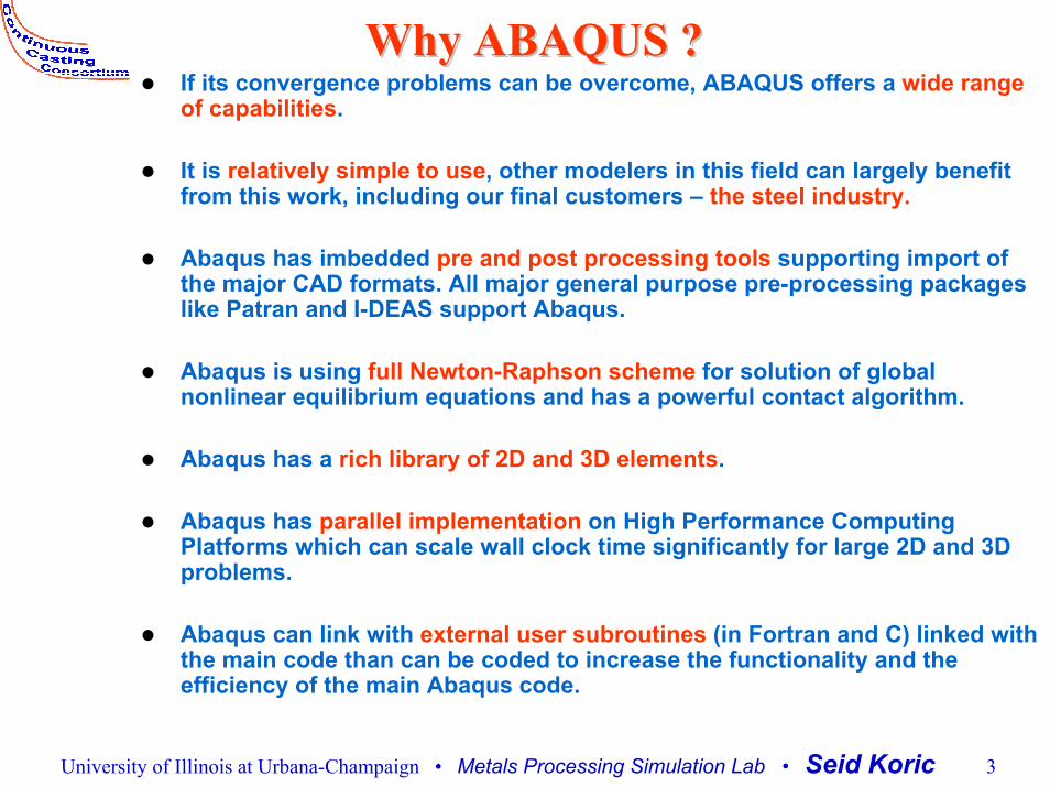
Comparison of Comparison of AbaqusAbaqus and CON2D for previous and CON2D for previous complex modelcomplex model

CON2D ABAQUS/Native ExplicitElement type 6 node triangular 4 node rectangularNumber of elements 400 300Number of nodes 1803 603Initial time step 1.E-4 1.E-11RAM used 350Mb 450MbWall clock on IBMp690 5 minutes 5760 minutes (96 hours)

D is ta n ce fro m s la b su rfa c e (m m )

Y-S

tress

(MP

a)

0 5 1 0 1 5 2 0 2 5 3 0-1 0

-5

0

A b a q u sC O N 2 D

4 3 s = > 1 m /m in

D IS T AN C E -F R O M -S LAB-S U R F AC E (m m )

STR

ES

S-Y

(MP

a)

0 10 20 30-7

-6

-5

-4

-3

-2

-1

0

1

2

3

4

5

C O N 2 D R e sultsAba qus results

5 se conds


Conclusions (Past Work):Conclusions (Past Work):

Nowadays, It is possible to perform numerical simulations of steel solidification process in the Continuous Casting Mold with multipurpose commercial finite element code-Abaqus.

~1000 x more CPU resources are needed with Abaqus explicit creep integration compared to in-house code CON2D for identical problem due to superior CON2D robust integration scheme

Main culprit for Abaqus slow performance is the integration of the in creep functions.

Abaqus native implicit creep integration has failed completely for this class of problems.

Quantitatively results are matching well, qualitative differences are under investigation.


Solutions to Solutions to AbaqusAbaqus Slow Performance Slow Performance Solution1: Apply Kozlowski III model everywhere (liquid and solid) through the CREEP subroutine with its explicit integration, and apply Abaqusnative perfect plasticity for liquid. Currently Abaqus Plasticity works only coupled with implicit creep integration. This issue has been addressed to HKS developers.

Solution 2: Replace Abaqus native local integration model with fully implict local integration from CON2D followed by its robust two level bounded NR integration scheme coded in another user defined subroutine UMAT. This work is currently under way. HKS has showed interest in our UMAT work.

Solution 2 is the focus of our current work !


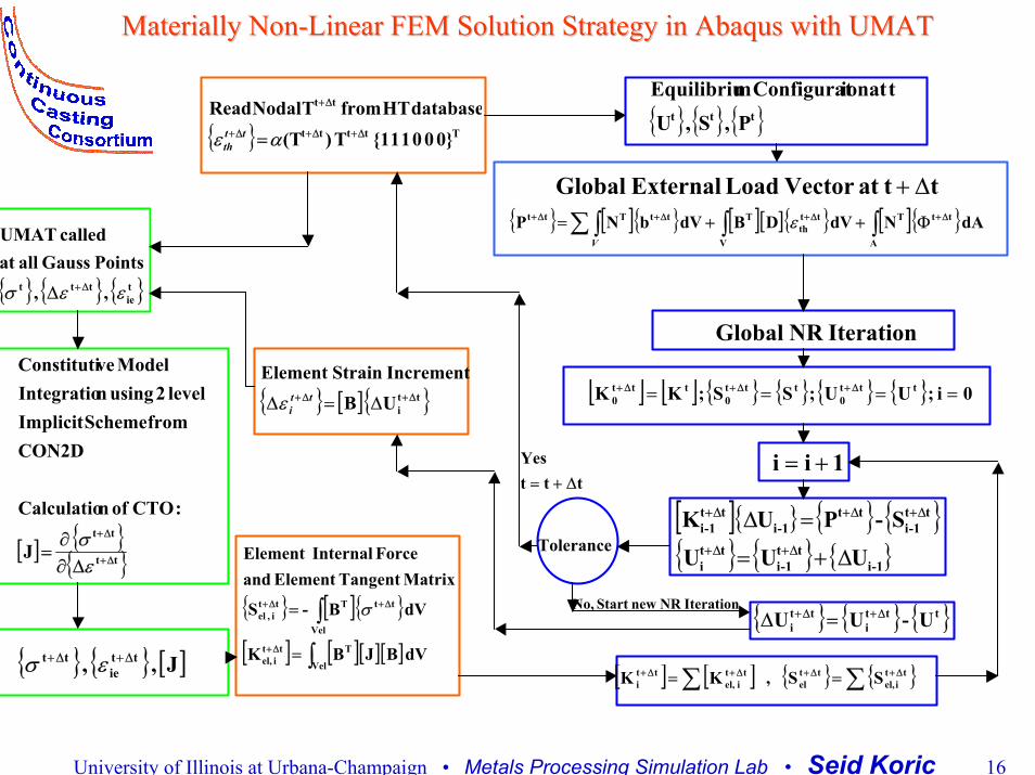
Materially NonMaterially Non--Linear FEM Solution Strategy in Linear FEM Solution Strategy in AbaqusAbaqus with UMATwith UMAT

IterationNR Global

[ ] [ ] { } { } { } { } 0i ; UU ; SS ; KK ttt0

ttt0

ttt0 ==== ∆+∆+∆+

1ii +=

[ ]{ } { } { }{ } { } { }-1i

tt-1i

tti

tt-1i

tt-1i

tt-1i

U U U

S - P U K

∆+=

=∆∆+∆+

∆+∆+∆+

Tolerance

{ } { } { }ttti

tti U - U U ∆+∆+ =∆

tt tYes

∆+=

IterationNR newStart No,

{ } [ ]{ } [ ][ ]{ } [ ]{ }dA N dV D B dV b N P tt

A

Tttth

V

TttTtt ∆+∆+∆+∆+ Φ++= ∫∫∑∫ εV

ttat Vector Load External Global ∆+

{ } { } { } P , S , Utat ionConfigurat mEquilibriu

ttt

{ } Ttttt

tt

0} 0 0 1 1 {1 T )(T database HT from T Nodal Read

∆+∆+∆+

∆+

=αε ttth

{ } [ ]{ }ttiU B

IncrementStrainElement ∆+∆+ ∆=∆ tt

iε

{ } { } { }tie

ttt , , Points Gauss allat

called UMAT

εεσ ∆+∆

[ ] { }{ }tt

tt J

:CTO of nCalculatio

CON2D from SchemeImplicit

level 2 using nIntegratioModel veConstituti

∆+

∆+

∆∂∂

=εσ

{ } { } [ ]J , , ttie

tt ∆+∆+ εσ

{ } [ ]{ }

[ ] [ ][ ][ ]dV B J B K

dV B- S

MatrixTangent Element andForceInternalElement

Vel

Ttti el,

tt

Vel

Ttti , el

∫

∫=

=

∆+

∆+∆+ σ

[ ] [ ] { } { }∑∑ ∆+∆+∆+∆+ == ttiel,

ttel

tti el,

tti S S , K K


lam6_5_9

Wall clock while keeping liquid creep function is ~25min,230x Improvement compared with Abaqus Native Explicit Integration, but still 5x slower then CON2D.

Elastic-Perfectly Plastic constitutive law with very low Yield Stress coded for liquid phase replacing aggressive creep function and avoiding its integration. This implementation is actually faster then CON2D, 4min for this problem size and more then 1000x faster then Abaqus native explicit creep integration.

Almost identical results for Stress Distribution for both cases with UMAT and Native Explicit Creep Integration

sec 8.6at onDistributi Stress yσ

Early Results with UMAT Early Results with UMAT


More work on validation of results and comparison with CON2D.

Add constitutive model for steels with delta-ferrite and temp dependant thermal linear expansion.

Move to 2D and perhaps 3D FE domains with Abaqus to increase process understanding.

Derive and add Consistent Tangent Operator for temperature to UMAT and fully couple HT and Stress analysis.

Add more Complexity (Physics) to the model: Internal BC with Ferrostatic Pressure, contact and friction between mold and shell, input mold distortion data, effects of superheat…

If there are enough dofs (3D), parallel Abaqus features can be applied (each time increment solved in parallel).

Future WorkFuture Work


New Engineering Computational Resources at the National Center For Supercomputing Applications at the University Of Illinois

Seid KoricEngineering Applications Analyst

http://www.ncsa.uiuc.edu

[email protected]


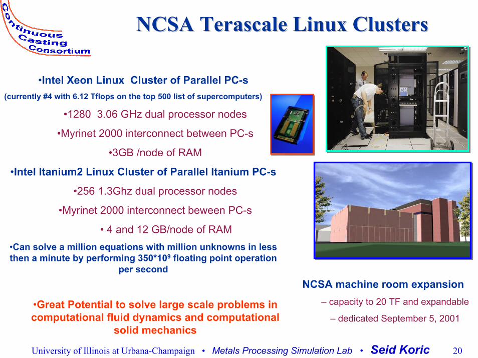
NCSA NCSA TerascaleTerascale Linux ClustersLinux Clusters

•Intel Xeon Linux Cluster of Parallel PC-s(currently #4 with 6.12 Tflops on the top 500 list of supercomputers)

•1280 3.06 GHz dual processor nodes

•Myrinet 2000 interconnect between PC-s

•3GB /node of RAM

•Intel Itanium2 Linux Cluster of Parallel Itanium PC-s

•256 1.3Ghz dual processor nodes

•Myrinet 2000 interconnect beween PC-s

• 4 and 12 GB/node of RAM•Can solve a million equations with million unknowns in less then a minute by performing 350*109 floating point operation

per second

•Great Potential to solve large scale problems in computational fluid dynamics and computational

solid mechanics

NCSA machine room expansion– capacity to 20 TF and expandable

– dedicated September 5, 2001


Shared Memory NCSA Capabilities: Shared Memory NCSA Capabilities:

•Shared memory systems IBM Regatta, Power 4•2+ TF of clustered SMP

•32 SMP CPUS, 1.3 Ghz

•large, 256 GB memory

•AIX IBM Unix OS

Perfect for engineering commercial software like:

Abaqus, Ansys, Fluent, LS-Dyna, Marc, PRO/E….

•Further SMP Expansions coming this year with newest SMP platform(s)

•Secondary and tertiary storage•500 TB secondary storage SAN

•3.4 PB tertiary storage


Computing in 21Computing in 21StSt Century, a story of Century, a story of TeraGridTeraGridComputing Resources: Anytime, AnywhereComputing Resources: Anytime, Anywhere

NCSA/UIUC

ANL

UICMultiple Carrier Hubs

Starlight / NW Univ

Ill Inst of Tech

Univ of Chicago

I-WIRE

StarLightInternational Optical Peering Point

(see www.startap.net)

Los Angeles

San Diego

TeraGrid Backbone

Abilene

Chicago

IndianapolisUrbana

OC-48 (2.5 Gb/s, Abilene)Multiple 10 GbE (Qwest)Multiple 10 GbE (I-WIRE Dark Fiber)

Qwest 40 Gb/s Backbone

$7.5M Illinois DWDM Initiative


0

5000

10000

15000

20000

25000

30000

Wall Clock (sec)

1 2 4 8

CPUS

Abaqus/Standard, SMP Solver, 1m dofs

IBM p690

HP Superdome

SGI O2K

Some CSM and CFD Applications on NCSA machines

WRF (Fixed Problem Size)

0.010

0.100

1.000

1 2 4 8 16 32 64 128

Number of Processors

Wal

l Clo

ck T

ime

(hou

rs)

TitanPlatinumCopperMercuryTungstenReference: Bob

Wilhelmson (NCSA)Severe Weather

Forecast


Acknowledgments:Acknowledgments:

Prof. Brian G. ThomasChungsheng Li, PhD, Former UIUC studentCaludio Ojeda, Former Visiting ScholarNational Center for Supercomputing Applications


Solidification Stress Model in Abaqusccc.illinois.edu/s/2004_Presentations/CCC2004_seid.pdf · CCC...

Documents

Transcript of Solidification Stress Model in Abaqusccc.illinois.edu/s/2004_Presentations/CCC2004_seid.pdf · CCC...