University of Central Florida University of Central Florida

STARS STARS

Honors Undergraduate Theses UCF Theses and Dissertations

2021

Small Business Risk In The Context of a Pandemic: A Simulation Small Business Risk In The Context of a Pandemic: A Simulation

Gregory J. Sperry University of Central Florida

Part of the Economics Commons, and the Entrepreneurial and Small Business Operations Commons

Find similar works at: https://stars.library.ucf.edu/honorstheses

University of Central Florida Libraries http://library.ucf.edu

This Open Access is brought to you for free and open access by the UCF Theses and Dissertations at STARS. It has

been accepted for inclusion in Honors Undergraduate Theses by an authorized administrator of STARS. For more

information, please contact STARS@ucf.edu.

Recommended Citation Recommended Citation Sperry, Gregory J., "Small Business Risk In The Context of a Pandemic: A Simulation" (2021). Honors Undergraduate Theses. 1010. https://stars.library.ucf.edu/honorstheses/1010

SMALL BUSINESS RISK IN THE CONTEXT OF A PANDEMIC:

A SIMULATION

by

GREGORY J. SPERRY

A thesis submitted in partial fulfillment of the requirements

for the Honors in the Major Program in Economics

in the College of Business

and in the Burnett Honors College

at the University of Central Florida

Orlando, Florida

Spring Term, 2021

Thesis Chair: Dr. Melanie Guldi

ii

Abstract

In this thesis, I consider the impact of the COVID-19 pandemic on small businesses, as

they are acutely at risk due to the lack of implicit government insurance that would be available

to larger corporations. I will discuss insurance's characteristics using the basic theory of

insurance, analyze pandemic insurance's viability in the private market, and critique alternative

solutions. While the theory suggests that pandemics are not insurable in the private market, I will

perform specific analysis to determine if this is the case or not. Using a simulation of the

economic landscape firms face, business owners with varying levels of risk aversion evaluate

whether or not to buy pandemic insurance. Specifically, I use the CRRA utility function to model

risk aversion and calculate the demand for insurance and the insurance company's viability. I

find that while the demand exists for a pandemic insurance product, being the counterparty is a

losing proposition in the wholly private insurance market. Future research evaluating alternative

solutions, including catastrophe bonds and potential public-private partnerships, is needed to

determine the most effective financing for small businesses for future pandemic events.

iii

Table of Contents

I. Introduction ........................................................................................................................................... 1

II. Literature Review .................................................................................................................................. 2

A. Insurance ........................................................................................................................................... 2

1. Risk ............................................................................................................................................... 2

2. Demand for Insurance ................................................................................................................... 3

3. Supply for Insurance and Model ................................................................................................... 6

4. Insurability of Risks ...................................................................................................................... 7

B. Alternative Solutions ...................................................................................................................... 12

1. Catastrophe (CAT) Bonds ........................................................................................................... 12

2. Public-Private Partnership........................................................................................................... 15

C. Summary ......................................................................................................................................... 16

III. Methodology ................................................................................................................................... 18

A. Data Generation .............................................................................................................................. 18

B. Calculations ..................................................................................................................................... 21

C. Outcomes ........................................................................................................................................ 22

IV. Results ............................................................................................................................................. 24

A. Risk Neutral Case ........................................................................................................................... 24

B. Risk Adverse Cases ......................................................................................................................... 25

V. Simulation Parameter Sensitivity Analysis ......................................................................................... 31

A. Uncorrelated Case ........................................................................................................................... 31

B. Small Business Size Distribution .................................................................................................... 33

C. Pandemic Chance ............................................................................................................................ 35

VI. Conclusion ...................................................................................................................................... 37

VII. Appendix ......................................................................................................................................... 41

VIII. References ....................................................................................................................................... 48

iv

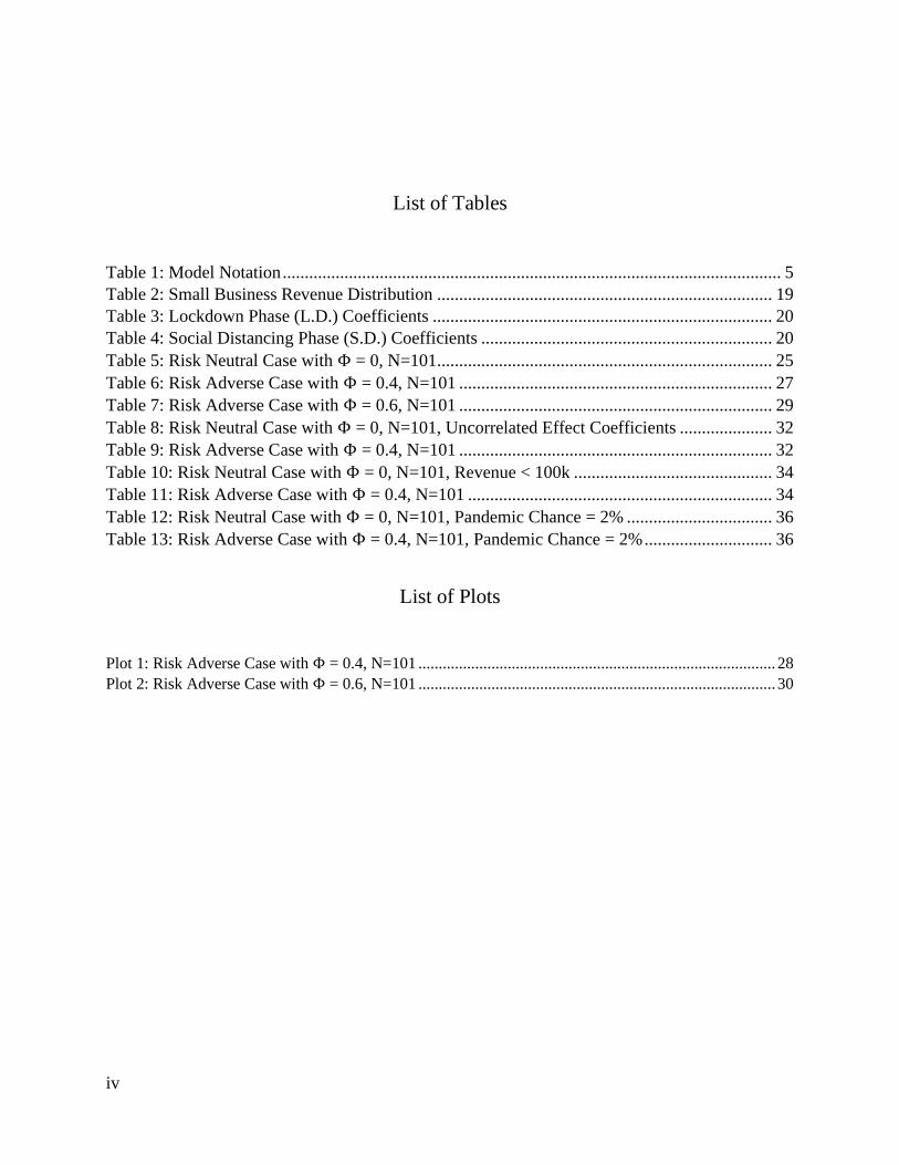
List of Tables

Table 1: Model Notation ................................................................................................................. 5

Table 2: Small Business Revenue Distribution ............................................................................ 19

Table 3: Lockdown Phase (L.D.) Coefficients ............................................................................. 20

Table 4: Social Distancing Phase (S.D.) Coefficients .................................................................. 20

Table 5: Risk Neutral Case with Φ = 0, N=101............................................................................ 25

Table 6: Risk Adverse Case with Φ = 0.4, N=101 ....................................................................... 27

Table 7: Risk Adverse Case with Φ = 0.6, N=101 ....................................................................... 29

Table 8: Risk Neutral Case with Φ = 0, N=101, Uncorrelated Effect Coefficients ..................... 32

Table 9: Risk Adverse Case with Φ = 0.4, N=101 ....................................................................... 32

Table 10: Risk Neutral Case with Φ = 0, N=101, Revenue < 100k ............................................. 34

Table 11: Risk Adverse Case with Φ = 0.4, N=101 ..................................................................... 34

Table 12: Risk Neutral Case with Φ = 0, N=101, Pandemic Chance = 2% ................................. 36

Table 13: Risk Adverse Case with Φ = 0.4, N=101, Pandemic Chance = 2% ............................. 36

List of Plots

Plot 1: Risk Adverse Case with Φ = 0.4, N=101 ........................................................................................ 28

Plot 2: Risk Adverse Case with Φ = 0.6, N=101 ........................................................................................ 30

1

I. Introduction

The COVID-19 pandemic has caused immense economic damage, especially to firms

offering products or services that preclude social distancing. Since firms did not predict the

current situation, it is understandable that most businesses did not have a pandemic risk

management solution in place. Or worse, many business owners thought their coverage under

general Business Interruption Insurance would apply to COVID-19. Unfortunately, thanks to the

response of the industry to the 2002-2003 SARS outbreak in China, many of these policies

explicitly exclude economic damage resulting from viruses (Ramnath 2020). Insurance

companies recognized the potential for these sorts of viruses to result in tremendous economic

disruptions. Accordingly, they added clauses to protect themselves from this sort of loss.

Furthermore, even if the clauses do not exclude pandemic loss, they typically require physical

damage for a claim to be filed. While businesses in emerging markets have access to quasi-

insurance instruments and programs to address pandemics, developed by both governmental and

non-governmental organizations, businesses in developed economies lack access. Consequently,

many US small businesses have suffered during the pandemic. This thesis will analyze

insurance's characteristics and determine pandemics' insurability in the private market using

simulated small business data and discuss catastrophe bonds and public private partnerships as

potential alternative solutions to private insurance.

2

II. Literature Review

A. Insurance

1. Risk

First, to discuss the idea of insurance, we must define risk. Henebry and Rejda (1995, 21)

note there are many different definitions of risk. For that reason, some choose to use the less

ambiguous term "loss exposure" instead, which Henebry and Rejda define as "any situation or

circumstance in which loss is possible, regardless of whether a loss occurs or not." Insurance

then is some scheme to transfer a loss exposure from one entity to another for a fee commonly

referred to as a premium.

Volumetric risk is the risk emergent from changing business conditions that cause a

decline in revenue. For example, Hofmann and Pooser (2017) identify how firms with exposure

to risk from weather events can hedge by buying weather derivatives, which are swap contracts

paying out based on the number of heating degree days or cooling degree days that occurred

relative to the terms set in the security. The applications are immediately apparent. Consider a

farmer growing strawberries who could have their entire crop decimated by too many heating

degree days (temperatures of less than 40°F). Such a farmer could buy a weather derivative that

pays out if a certain number of heating degree days occur to offset the financial pain of losing an

entire crop. Using a derivative in this manner causes them to function as a kind of insurance

administrated directly between a party seeking coverage and the capital suppliers. Of course,

pandemics have the potential to be a highly volumetric risk, as shown by the United States GDP

falling by a staggering 32.9% in the second quarter of 2020 (U.S. Bureau of Economic Analysis).

3

This massive reduction does not show the whole story as some industries have experienced an

even more significant revenue loss. Take the case of tourism or hospitability, especially early in

the pandemic, these industries ground to a screeching halt. Pandemic risk, in general, is

incredibly volumetric, and high-risk industries such as these only more so.

2. Demand for Insurance

When a small business or individual encounters a loss exposure that they find unacceptable,

they turn to insurance to mitigate that risk. Insurance can also be made compulsory in the interest

of public policy. Take automobile insurance, for example. It is a requirement for those who wish

to drive to be insured because most individuals cannot cover the losses or damages resulting from

an automobile accident. Small businesses with loans may be required to hold certain types of

insurance as a condition of the loan to ensure that even if a significant loss event occurs, the lender

can be made whole. Therefore, the risks agents find unacceptable to carry drive the demand for

insurance in nonmandated areas.

This concept can be made more rigorous by analyzing the situation through the lens of

utility theory. Imagine a customer has an automobile with a value of $25,000 and a 5% estimated

probability of suffering an accident that totals the vehicle. Multiplying these results in an expected

payout of $12501 if a consumer accepts a full insurance (that is to say, 100% loss coverage) policy.

Insurers often charge a premium equal to this expected payout, plus some "loading" fees for

administration and capital (Klein 2014). At first glance, there appears to be a contradiction since

it would not make sense for a person to enter into a contract with a negative expectation. Klein

1 $25,000 (𝑙𝑜𝑠𝑠 𝑒𝑥𝑝𝑜𝑠𝑢𝑟𝑒) ∗ 0.05 (𝑝𝑟𝑜𝑏𝑎𝑏𝑖𝑙𝑖𝑡𝑦 𝑜𝑓 𝑙𝑜𝑠𝑠 𝑜𝑐𝑐𝑢𝑟𝑟𝑖𝑛𝑔) = $1250

4

uses the example of betting $1 to win less than a dollar on a coin flip, which makes it easy to see

that insurance contracts will have a negative monetary expectation in absolute terms (2014).

A simple model of the expected utility of insurance an individual will receive is defined as

follows: First, small business owners who are risk-averse will have a utility function that is

increasing for wealth, but at a decreasing rate; call this function 𝑢∗. We can also use a basic utility

framework to demonstrate that risk-averse individuals will give up some wealth to avoid risk.

Assume that individuals derive utility only from wealth and are risk averse. If small businesses are

risk-averse, there are diminishing marginal returns on wealth for them. Then, the utility

function 𝑈(𝑊), will be increasing in wealth (𝑈′(𝑊) > 0) at a decreasing rate (𝑈′′(𝑊) < 0)

(Bhattachayra, Hyde, and Tu, 2013). Given these assumptions, the utility from a certain income

will be higher than the expected utility from an uncertain income, even when the expected income

is the same as the guaranteed income. Then π refers to the probability a loss of size 𝐿 occurs. 𝑊 is

the base state or wealth given no loss occurs. 𝑃 is the premium paid, a function of the amount of

coverage, 𝐶.

Understanding the demand for insurance from here requires us first to define the buyer's

wealth, which given our assumption that the loss will either occur for the total value of L or not at

all, we have 𝑊0 for the no insurance, no loss case. Continuing to the no insurance, loss case we

find 𝑊0 − 𝐿. For insurance, no loss case, we have 𝑊0 − 𝑃 and finally for the insurance loss case

we have 𝑊0 − 𝐿 − 𝑃 + 𝐶 (Ray and Achim 2008). Table 1 below contains all of the variables

defined in the model and a simple description. The critical insight here is to compare the effect of

insurance on the buyer's wealth. Insurance gives buyers the ability to transfer wealth from their

5

no-loss case to their loss case and reduces the variability between these two cases. Ray and Achim

define this transaction as "state-contingent wealth" and then the demand for insurance can be

thought of as demand for state-contingent wealth. Finally, the model of expected utility is:

𝐸[𝑢] = (1 − π)u(W − P(C)) + πu(W − P(C) − L + C) (Ray and Achim 2008).

Compared with the utility derived from a guaranteed change in wealth:

𝑈[𝐸(𝑊)] = 𝑈[(1 − π)(W − P(C)) + π(W − P(C) − L + C)]

Risk adverse agents prefer outcomes with a certain lower expected value as opposed to outcomes

with a higher but uncertain expected value. Insurance functions as a means to equalize utility

between the adverse and base states, and this arises from

Table 1: Model Notation

SYMBOL DESCRIPTION

𝒖 Risk-averse utility function

𝛑 Probability of loss

𝑳 Size of loss

𝑾 Wealth given no loss

𝑷 Premium paid

𝐂 Coverage

As applied to pandemic insurance, the demand for insurance results from how likely a

business owner finds the risk of a pandemic occurring to be and the damage expected. However,

given a pandemic of sufficient magnitude, the government will likely be forced to respond. As

stated, small businesses without access to implicit government insurance, the "too big to fail"

phenomenon, are the likely target market for this sort of product. Concerningly, a survey sent out

to North American small businesses found the representative small business only had two weeks

6

of cash reserves (Bartik et al., 2020). These low cash reserves suggest that small businesses are

not only unable to withstand even short term shutdowns, but also unlikely to be able to afford

pandemic insurance.

A risk-averse owner will value protecting the income they already have over risking that

income to secure a small amount of marginal income if the marginal utility of additional income

is decreasing. They will receive more utility from conserving the wealth they already have than

they will from receiving additional wealth. This follows from the second derivative of the utility

function for wealth. Given that a small business owner's income is likely to equal to the profit their

small business earns, it follows that small businesses may be more risk-averse than in the

traditional framework that assumes firms only maximize profit. Indeed, the more risk-averse an

agent is, the greater their demand for insurance. Small business owners who derive their entire

income from their business's profit are likely to be highly risk averse and therefore have a high

demand for insurance.

3. Supply for Insurance and Model

The conditions have now been established for when a party will purchase insurance. How

will the firms that supply this insurance be structured? What price will they charge? Firms here

are assumed to be risk-neutral, as in the seminal paper by Rothschild and Stiglitz (1976). This

assumption makes intuitive sense, as insurance companies are owned by agents with differing asset

allocations and risk tolerances. By and large, an insurance company is owned by many, highly

diverse people. Comparatively, the average small business is owned by few incredibly diversified

individuals. From this, we know the utility function 𝑈(𝑊) of an insurance company must have:

7

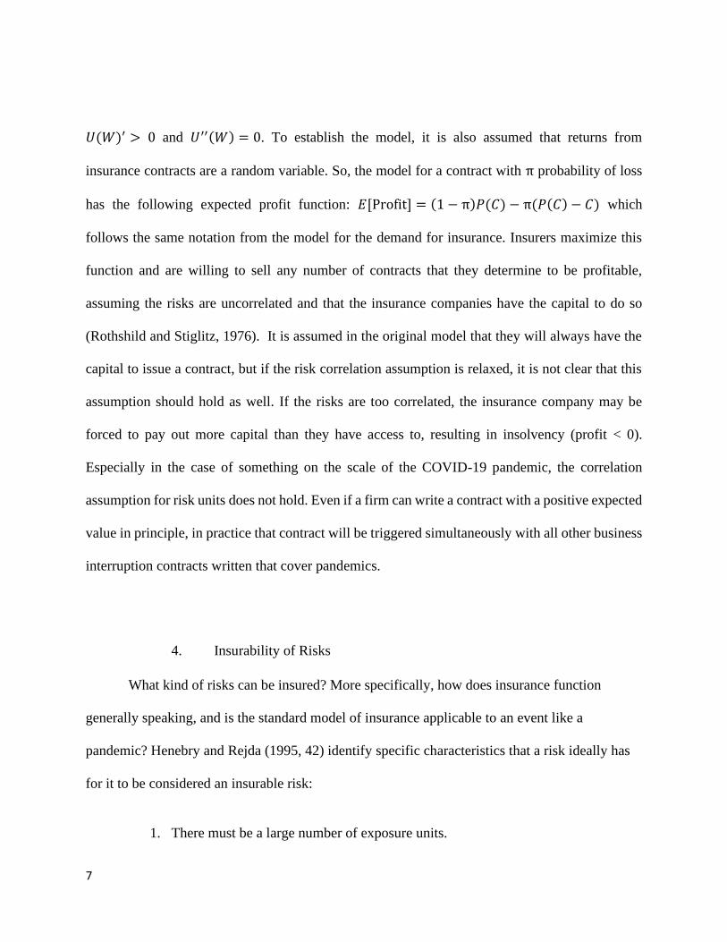
𝑈(𝑊)′ > 0 and 𝑈′′(𝑊) = 0. To establish the model, it is also assumed that returns from

insurance contracts are a random variable. So, the model for a contract with π probability of loss

has the following expected profit function: 𝐸[Profit] = (1 − π)𝑃(𝐶) − π(𝑃(𝐶) − 𝐶) which

follows the same notation from the model for the demand for insurance. Insurers maximize this

function and are willing to sell any number of contracts that they determine to be profitable,

assuming the risks are uncorrelated and that the insurance companies have the capital to do so

(Rothshild and Stiglitz, 1976). It is assumed in the original model that they will always have the

capital to issue a contract, but if the risk correlation assumption is relaxed, it is not clear that this

assumption should hold as well. If the risks are too correlated, the insurance company may be

forced to pay out more capital than they have access to, resulting in insolvency (profit < 0).

Especially in the case of something on the scale of the COVID-19 pandemic, the correlation

assumption for risk units does not hold. Even if a firm can write a contract with a positive expected

value in principle, in practice that contract will be triggered simultaneously with all other business

interruption contracts written that cover pandemics.

4. Insurability of Risks

What kind of risks can be insured? More specifically, how does insurance function

generally speaking, and is the standard model of insurance applicable to an event like a

pandemic? Henebry and Rejda (1995, 42) identify specific characteristics that a risk ideally has

for it to be considered an insurable risk:

1. There must be a large number of exposure units.

8

2. The loss must be accidental and unintentional.

3. The loss must be determinable and measurable.

4. The loss should not be catastrophic.

5. The chance of loss must be calculable.

6. The premium must be economically feasible.

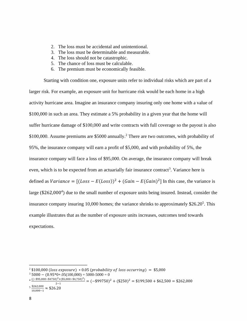
Starting with condition one, exposure units refer to individual risks which are part of a

larger risk. For example, an exposure unit for hurricane risk would be each home in a high

activity hurricane area. Imagine an insurance company insuring only one home with a value of

$100,000 in such an area. They estimate a 5% probability in a given year that the home will

suffer hurricane damage of $100,000 and write contracts with full coverage so the payout is also

$100,000. Assume premiums are $5000 annually.2 There are two outcomes, with probability of

95%, the insurance company will earn a profit of $5,000, and with probability of 5%, the

insurance company will face a loss of $95,000. On average, the insurance company will break

even, which is to be expected from an actuarially fair insurance contract3. Variance here is

defined as 𝑉𝑎𝑟𝑖𝑎𝑛𝑐𝑒 = [(𝐿𝑜𝑠𝑠 − 𝐸(𝐿𝑜𝑠𝑠))2 + (𝐺𝑎𝑖𝑛 − 𝐸(𝐺𝑎𝑖𝑛)2] In this case, the variance is

large ($262,0004) due to the small number of exposure units being insured. Instead, consider the

insurance company insuring 10,000 homes; the variance shrinks to approximately $26.205. This

example illustrates that as the number of exposure units increases, outcomes tend towards

expectations.

2 $100,000 (𝑙𝑜𝑠𝑠 𝑒𝑥𝑝𝑜𝑠𝑢𝑟𝑒) ∗ 0.05 (𝑝𝑟𝑜𝑏𝑎𝑏𝑖𝑙𝑖𝑡𝑦 𝑜𝑓 𝑙𝑜𝑠𝑠 𝑜𝑐𝑐𝑢𝑟𝑟𝑖𝑛𝑔) = $5,000 3 5000 − (0.95*0+.05(100,000) = 5000-5000 = 0

4 ((−$95,000−$4750)2+($5,000−$4,750)2)

2−1= (−$99750)2 + ($250)2 = $199,500 + $62,500 = $262,000

5 $262,000

10,000−1≈ $26.20

9

In the case of a pandemic, there are many exposure units as a pandemic affects any

business unable to operate under social distancing constraints. However, this differs from

traditional insurance markets as the exposure units are highly correlated. Specific industries, such

as restaurants and hospitality, represent many exposure units, but all of these exposure units will

file claims simultaneously. Therefore, the exposure unit condition is deceptive. It appears at first

glance that it is satisfied but depending on the industry makeup of the businesses insured, there

could be more claims than is standard for a given number of exposure units and loss probability.

Condition two, which requires a loss be accidental and unintentional, presents a challenge

when considering the contract's exact specification. Firm owners have control over their

operating conditions and may cut operating hours more sharply when they can offload some or

all of the lost revenue to a third party. More specifically, they have a perverse incentive to

operate their business as little as the insurance contract allows while maintaining similar

effective profit when the insurance is considered. Given a contract that replaces all lost revenue,

firm owners can avoid themselves contracting the disease or perhaps more critically, avoid

potential liability claims from employees that contract the disease while working for the

business.

Condition three, or the measurability and determinability of the loss, clearly requires

predicting in advance the magnitude of a pandemic, which presents significant challenges. A

model would have to consider many variables, including duration, severity, and contagiousness,

among others. Furthermore, even if government regulation allows for a particular activity or

10

business to operate during a pandemic, consumers must feel confident that they will be safe. This

uncertainty makes modeling the exact amount of loss difficult before the fact.

For instance, a restaurant operating under a stay-at-home order will face a substantial

reduction in revenue but perhaps can make some of that up with takeout orders and other

alternatives to sit-down dining. How was an insurance adjuster supposed to predict with accuracy

this alternative business line's success in mitigating losses? If they underestimate this mitigation

technique's effect, the premiums they charge may not be affordable by an industry already

known for infamously tight margins. However, if they overstate the effect, the premium charged

may not be enough to cover the value of the claims they must pay. As a result of the COVID-19

pandemic, there are now estimates adjusters will use. However, these estimates are based on this

pandemic's specific conditions and are not likely to be perfectly applicable to future ones.

Nevertheless, this condition is more viable for future pandemics than it was for COVID-19.

Condition four, the non-catastrophe requirement, is perhaps the most significant

impediment to pandemic insurance, as pandemics on the scale of COVID-19 have the potential

to go from merely catastrophic to cataclysmic. Cutler and Zeckhauser (1997) distinguish

between catastrophe and cataclysms, albeit with a – by their admission – arbitrary standard of

"5+ billion dollars". Nevertheless, the paper uses the concept to explore catastrophes that are so

large in scale the traditional insurance market breaks down, instead relying on alternative

solutions such as government intervention. A solution exists for large firms in the existing

framework, namely government bailouts and extremely favorable term bailout loans. These firms

considered "too big to fail" have a sort of implicit insurance and have no need for this sort of

11

product. Small businesses that are much less likely to receive this sort of treatment are the

primary focus of this thesis.

Condition five, the loss's calculability, has been tackled already by the insurance industry

for influenza pandemics. An exceedance probability analysis in Pandemics: Risk, Impacts, and

Mitigation found that there was a 1% chance in any given year of a global influenza pandemic

that resulted in 6+ million deaths (Madhav et al., Chapter 17, 2017). However, if the insurance

contract provides coverage for any pandemic, not just those caused by influenza, the probability

of loss may be marginally greater. Insurers must keep this slight potential for variability in mind.

For condition six, which requires that the market can bear the insurance companies'

premiums, the economic feasibility will depend on what the insurance company estimates to be

the chance of loss and how they handle the uncertainty regarding the loss's magnitude. The

premiums could be priced such that only the businesses most susceptible to interruption by

pandemics will be interested in purchasing the insurance, resulting in a substantial adverse

selection in the insurance market. Adverse selection occurs when asymmetric information

between the insurance company and the insured firm leads to the insurance company selling

insurance at a price that does not accurately capture the risk they are taking on (Henebry and

Rejda, 1995, 23). Overall, the condition is difficult to determine without modeling pandemic

insurance, which is part of what this thesis intends to accomplish.

Finally, given the problems presented by the insurability conditions related to the

magnitude and measurability of the loss associated with a pandemic, private market insurance is

likely not viable as a solution. The correlation of exposure units can be incredibly high, and

12

predicting these exposure units' claim amount involves a host of assumptions. There is a

considerable risk of making an incorrect assumption and drastically distorting the contract's

value an insurance company has written relative to its actual value. By their very nature,

pandemics are likely not an insurable risk in the private market without particular conditions. So,

I have demonstrated that traditional insurance may not be a good solution for pandemics due to

the conditions of insurability discussed. I proceed below by detailing alternatives to traditional

insurance.

B. Alternative Solutions

1. Catastrophe (CAT) Bonds

One of the most significant challenges I just identified for insuring pandemics is their

potential to be catastrophic in the loss's size. A single insurance company may not have the

capital on hand to pay out all of the claims, which will arrive all at once due to the highly

correlated nature of the underlying risk. To distribute this risk, some financial instrument that

provides financing in the event of the loss occurring is required, which is the catastrophe or CAT

bond. CAT bonds represent a way for an insurance company to partially diversify themselves

while insuring events with highly correlated risk units, which certainly includes pandemics. If an

insurer chooses to insure catastrophic events, they must have a plan in place to be able to respond

to the huge quantity of claims that arise at once due to the nature of the event. CAT bonds can

function as one tool in such a risk management solution.

Catastrophe bonds refer to derivatives that payout given a catastrophe occurs. They help

keep insurers solvent during widespread and exceptionally damaging events, such as hurricanes

and wildfires. This is part of a process known as reinsurance (Insurance Information Institute

13

2020). Reinsurance is paramount in the insurance industry – accounting for more than 25% of

the premium proceeds collected (Adiel 1996). A financial instrument's payout based on crossing

a specific indicator is referred to as a parametric trigger (Edesess, 2015). The chief advantage of

parametric triggers as opposed to indemnity or industry loss, the two other common types of

triggers used in CAT bonds, is the speed at which payouts can occur. According to Polacek's

(2018) calculations using data from Artemis (a financial company specializing in utilizing capital

markets to transfer disaster risk), parametric triggers payout on average in just three months,

compared to indemnity triggers at a staggering two to three years.

Before the current pandemic, less impactful diseases such as Ebola in 2014 and SARS in

early 2003 threatened the world economy. Informed by this, World Bank recognized the

challenges in securing just-in-time financing for pandemic responses in developing countries. It

launched the Pandemic Emergency Financing Facility in 2016 (World Bank, 2020). Shortly

after, bonds were issued with trigger conditions designed to provide relief for countries

supported by the International Development Association (IDA), the World Bank's policy arm

responsible for global economic development. The triggers are as follows, and all four must be

present in order for the securities to payout:

1. Outbreak size [all three sub-triggers must be met]:

• The rolling (or ongoing) total case amount reaches 250 or more.

• The total number of fatalities reaches 250 in IDA/IBRD countries (countries

identified as both poor and creditworthy that are eligible to receive loans)

• At least 12 weeks have passed from the start of the outbreak.

2. The confirmation ratio: confirmed cases as a percentage of total cases must

exceed 20%

14

3. Cross-border spread: the outbreak needs to be in more than one country, each

having had 20 or more fatalities.

4. Positive growth rate: the total number of cases in IDA countries must be growing

at an exponential rate as confirmed by the third-party calculation agent (AIR

Worldwide).

AIR Worldwide, an independent third-party contractually responsible for determining the

bonds' status, confirmed all four of these triggers on April 17, 2020, and the bonds started to

disperse money to IDA countries to provide relief for the COVID-19 pandemic. These securities

represent an attempt to mitigate pandemic risk in the context of international development, but

clearly, there are more areas in which adequate structures did not exist to address pandemic risk.

However, the payout time of only two months, a below-average amount of time for parametric

trigger bonds, was still considered too slow, and World Bank has abandoned them for future

pandemic financing (Brenton Woods Project, 2020).

The advantages of CAT bonds or other disaster derivatives are apparent for those using

them to hedge risk or, in the case of World Bank, relief funding, but why would a counterparty

find these to be an attractive investment? After all, predicting these events is not possible, so

upon first glance, it appears these investors are merely putting their chips on "minor hurricanes

this year" or the like without a sound strategy. However, as Edesess (2015, 6) notes, "the risks

they [CAT bonds] cover are virtually uncorrelated with other risks such as equity market risk,

interest rate risk, and credit risk." Therefore, an investor with considerable exposure to

traditional markets could use them to diversify their portfolio as part of a risk management

strategy.

15

While a sound system for other disasters, investors in World Bank's Pandemic Bonds saw

this strategy fail. The investors lost their money in the World Bank bonds as those funds were

used to provide relief to developing countries, as specified in the terms of the contract.

Unfortunately for the investors, unlike other disasters, COVID-19 resulted in a massive stock

market crash in the pandemic's early stages. Therefore, these investors saw instruments they

expected to be uncorrelated with overall equity markets plunge simultaneously as the equity

market. Baker et al. (2020) have suggested that this resulted from the widespread lockdowns

enacted by governments almost universally to contain the virus's spread. Future securitization of

pandemics seems unlikely given that traditional investors and institutions will likely no longer

view CAT bonds tracking pandemics as effective hedges to equity markets.

2. Public-Private Partnership

Given the sheer magnitude of pandemics, and the likely higher correlation of risk units

compared to even other catastrophic events, traditional reinsurance markets may fail to

adequately cover insurers operating in this space. For a given risk, the government can function

as a reinsurer of last resort if there is a significant publish interest in providing insurance for that

risk. As seen by British terrorism reinsurance and American flood reinsurance, this structure has

already been implemented to cover similar events the private market deems uninsurable.

Following the 1993 Provisional IRA's acts of terrorism, insurance companies added exceptions

for damage caused by terrorism. The U.K. government created a reinsurance scheme backed with

the full force of the treasury entitled PoolRe. Essentially, individual insurers agree to offer

terrorism insurance, pay a premium to PoolRe that is a fraction of terrorism-related claims, and

then PoolRe picks up the slack. Should the reserves be exhausted, the British government will

16

issue a loan for the remaining balance, which will be paid back over time using the premiums

collected by primary insurers (PoolRe 2019).

For the case of pandemics, the government can set up a program, funded by a tax on

businesses, that offers insurance in the event a pandemic occurs. Government can prevent

adverse selection by simply requiring businesses to purchase the insurance, whether or not they

would do so independently. The exact structure of this program is an area for future research, as

any policy taxing an already vulnerable institution like the small business must be crafted

carefully to avoid it out of existence. For example, instead of an additional tax, the funding could

come from taxes already paid by the small business. Direct transfers from the government can

also be considered, such as the Paycheck Protection Program in the US. Or, could be expanded

to include other types of insurance that firms typically carry. This would offset the tax by

eliminating the need for other types of premiums. The insurance company could administer the

program and be responsible for a predetermined amount of liability, and the government would

be liable for the rest as a reinsurer. Since the underlining private market issuers of pandemic

insurance are related to the magnitude of the loss, the government's addition to cover the losses

beyond reasonable for the insurance firm provides a solution. This is a very natural fit, as the

government already has an incentive to protect businesses to preserve tax revenue in the future

and current jobs.

C. Summary

In this literature review, I have discussed first risk and then insurance generally,

developing the theory and enumerating the conditions required for an event to be insurable.

17

Then, I applied the theory to the pandemic case and discussed some of the problems that arise.

Finally, I discussed public and private market mitigation methods for the issues presented. As

interesting as these hypothetical solutions are, they are complex to model and require

assumptions due to how theoretical it all is. Instead, I will proceed by focusing on the viability of

private market pandemic insurance. This question is answerable by using the theory of insurance

demand developed and applying it to business owners with varying risk aversion levels.

18

III. Methodology

A. Data Generation

Due to the recency of the pandemic, complete data on the economic impacts have not

been collected. Therefore, to analyze the viability of private market pandemic insurance,

simulated data based on assumptions from the available research is the next best alternative.

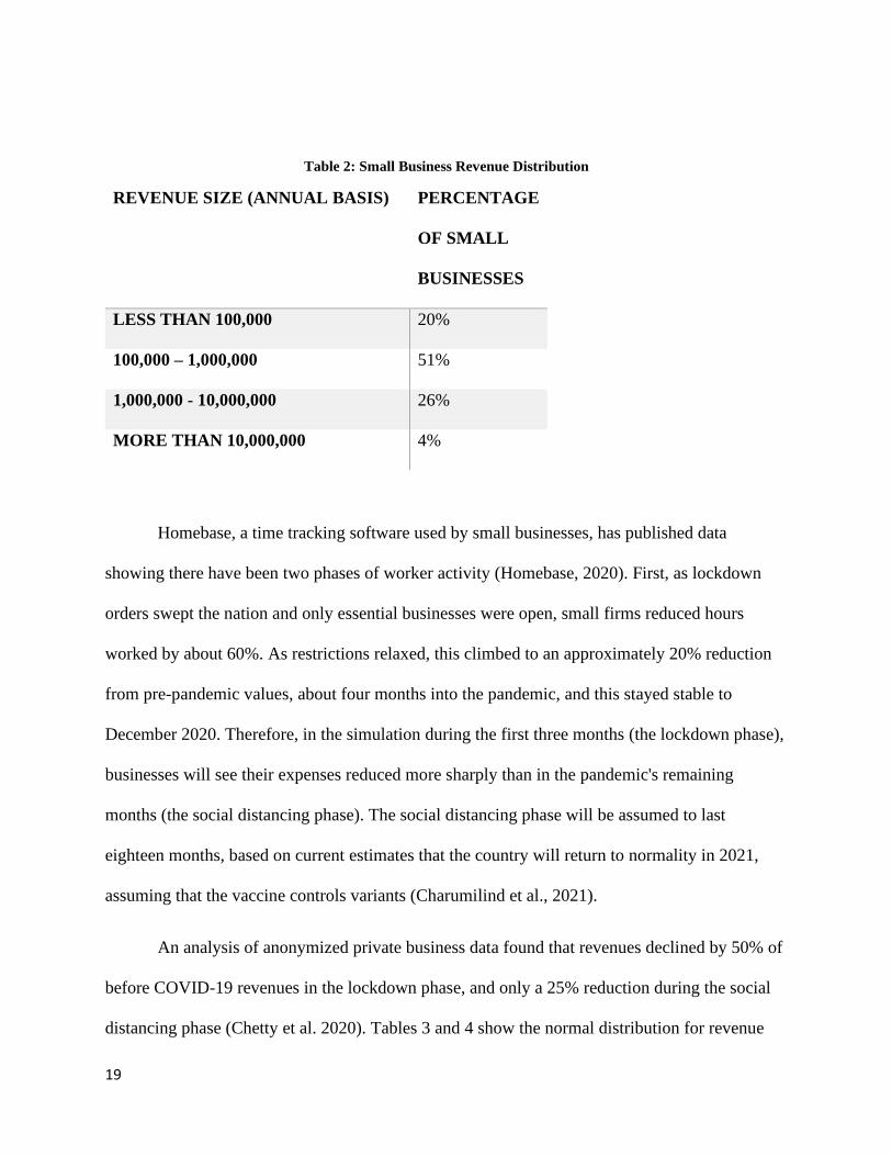
First, businesses are generated with a base yearly revenue. A small business for these

purposes is defined as having less than 500 employees. The businesses used in the simulation

will be distributed according to the following percentages and revenue breakdowns, collected

in the Small Business Annual Credit Report (Federal Reserve, 2019). These percentages,

displayed below in Table 2, do not add to 100%, as the original data was presented already

rounded. This is addressed in the simulation by scaling the sample size up slightly from the

initial value. From here, revenue and expenses during the pandemic will be calculated as

specified in the Calculations section. After finding these values, I will consider insurance that

fully covers the lost revenue during the pandemic and evaluate the demand for insurance

using a constant relative risk aversion (CRRA) utility function for the firm owners.

19

Table 2: Small Business Revenue Distribution

REVENUE SIZE (ANNUAL BASIS) PERCENTAGE

OF SMALL

BUSINESSES

LESS THAN 100,000 20%

100,000 – 1,000,000 51%

1,000,000 - 10,000,000 26%

MORE THAN 10,000,000 4%

Homebase, a time tracking software used by small businesses, has published data

showing there have been two phases of worker activity (Homebase, 2020). First, as lockdown

orders swept the nation and only essential businesses were open, small firms reduced hours

worked by about 60%. As restrictions relaxed, this climbed to an approximately 20% reduction

from pre-pandemic values, about four months into the pandemic, and this stayed stable to

December 2020. Therefore, in the simulation during the first three months (the lockdown phase),

businesses will see their expenses reduced more sharply than in the pandemic's remaining

months (the social distancing phase). The social distancing phase will be assumed to last

eighteen months, based on current estimates that the country will return to normality in 2021,

assuming that the vaccine controls variants (Charumilind et al., 2021).

An analysis of anonymized private business data found that revenues declined by 50% of

before COVID-19 revenues in the lockdown phase, and only a 25% reduction during the social

distancing phase (Chetty et al. 2020). Tables 3 and 4 show the normal distribution for revenue

20

and expenses during both the lockdown and social distancing phases, respectively. To model the

relationship between the two phases, the social distancing phase coefficients will be generated

from the lockdown phase coefficients with a correlation value of 0.8. This assumption is made to

ensure there are not overly large swings between the two phases. A business with a coefficient

on the left tail of the lockdown phase distribution should not have a social distancing coefficient

on that distribution's right tail. The correlation value is relatively strong but not perfect. A perfect

correlation would imply that the subsequent phase's performance can be predicted precisely from

the first, which is not a realistic assumption.

Table 3: Lockdown Phase (L.D.) Coefficients

EFFECT DISTRIBUTION

EXPENSES ~ N(-.6, .01)

REVENUE ~ N(-.6, .01)

Table 4: Social Distancing Phase (S.D.) Coefficients

EFFECT DISTRIBUTION

EXPENSES ~ N(-.2, .01)

REVENUE ~ N(-.25, .01)

An average profit margin for small enterprises of 7.0% was found in an operating

analysis of small businesses. (Government of Canada, 2015). While not computed from U.S.

firms, this figure is still a reasonable estimate for the mean of the normal distribution by which

profit margin will be distributed in the simulation, Profit Margin ~ N (0.07, 0.09).

21

B. Calculations

After base annual revenue, profit margin, and the phase-based effect coefficients for both

revenue and expenses have been generated according to the specified distributions,

(1) 𝑀𝑜𝑛𝑡ℎ𝑙𝑦 𝑅𝑒𝑣𝑒𝑛𝑢𝑒 = 𝐴𝑛𝑛𝑢𝑎𝑙 𝑅𝑒𝑣𝑒𝑛𝑢𝑒/12. From the profit margin equation

(2) 𝑃𝑟𝑜𝑓𝑖𝑡 𝑀𝑎𝑟𝑔𝑖𝑛 =𝑅𝑒𝑣𝑒𝑛𝑢𝑒−𝐸𝑥𝑝𝑒𝑛𝑠𝑒𝑠

𝑅𝑒𝑣𝑒𝑛𝑢𝑒, monthly expenses can be found by solving this equation

for expenses, which yields (3) 𝑀𝑜𝑛𝑡ℎ𝑙𝑦 𝐸𝑥𝑝𝑒𝑛𝑠𝑒𝑠 = −𝑃𝑟𝑜𝑓𝑖𝑡 𝑀𝑎𝑟𝑔𝑖𝑛 ∗ 𝑀𝑜𝑛𝑡ℎ𝑙𝑦 𝑅𝑒𝑣𝑒𝑛𝑢𝑒 +

𝑀𝑜𝑛𝑡ℎ𝑙𝑦 𝑅𝑒𝑣𝑒𝑛𝑢𝑒. Monthly profit is of course simply the difference between (1) and (3). Monthly

revenue during the lockdown phase is calculated by (4) 𝑀𝑜𝑛𝑡ℎ𝑙𝑦 𝑅𝑒𝑣𝑒𝑛𝑢𝑒 +

(𝑀𝑜𝑛𝑡ℎ𝑙𝑦 𝑅𝑒𝑣𝑒𝑛𝑢𝑒 ∗ 𝑅𝑒𝑣𝑒𝑛𝑢𝑒 𝐸𝑓𝑓𝑒𝑐𝑡 𝐶𝑜𝑒𝑓𝑓𝑖𝑐𝑒𝑛𝑡 𝐿𝐷). Expenses are calculated the same way

as in (4), simply replacing revenue for expenses. The formula for the social distancing phase is

identical to (4) but with the social distancing effect coefficient instead. Profit values for each phase

are calculated using the difference between monthly revenue and monthly expenses. Finally, the

total revenue effect is calculated as (𝑀𝑜𝑛𝑡ℎ𝑙𝑦 𝐿𝐷 𝑅𝑒𝑣𝑒𝑛𝑢𝑒 ∗ 3 + 𝑀𝑜𝑛𝑡ℎ𝑙𝑦 𝑆𝐷 𝑅𝑒𝑣𝑒𝑛𝑢𝑒 ∗ 18).

Next, the insurance company is considered. The insurance company will be assumed to write

actuarially fair insurance contracts in the base model and be risk neutral, maximizing profit. The

coverage is full, so the insurance payout is equal to 𝑇𝑜𝑡𝑎𝑙 𝑅𝑒𝑣𝑒𝑛𝑢𝑒 𝐸𝑓𝑓𝑒𝑐𝑡. The monthly payout is

this value amortized throughout the pandemic, which is twenty-one months. The probability of a

pandemic is estimated at 1% (Madhav et al., Chapter 17, 2017). Therefore, monthly premiums are

calculated as 𝑀𝑜𝑛𝑡ℎ𝑙𝑦 𝑃𝑎𝑦𝑜𝑢𝑡 ∗1%

12∗ 𝐿𝑜𝑎𝑑𝑖𝑛𝑔 𝐹𝑒𝑒. Loading fee is treated as an independent

variable but is chosen to be zero in the base model.

22

Finally, the effect on profitability is considered for the outcomes of a firm either having or

not having insurance and a pandemic occurring or not occurring. If a firm has insurance but a

pandemic not occurring, the firm earns its monthly profit less the premium paid. If a pandemic does

occur when the firm has insurance, the firm receives their monthly profit given a pandemic occurred,

plus the insurance payout. Of course, in the no pandemic, no insurance case the profit is simply

monthly profit. Lastly, if there is a pandemic and the firm has no insurance, the firm receives their

monthly profit (or very likely loss in this instance) under pandemic conditions.

C. Outcomes

The firm owner will derive their income from the profit of their business. In some models, these

owners will be assumed to be risk-neutral, and in others, risk-averse. Because an owner could

receive a negative profit, in order to assume risk aversion, some utility function must be identified,

which can coherently handle negative values. Archetypal risk-averse functions, such as 𝑈 = ln(𝑥)

or 𝑈 = √𝑥 clearly have domain restrictions that make them unusable. Linear transformation of profit

was considered but ultimately rejected due to the distorting effects on the traditional examples of

risk-averse utility functions. Instead, the isoelastic utility function or constant relative risk aversion

(CRRA) is used (Barseghyan et al. 2018). The CRRA function is a piecewise function defined as

𝑈(𝑥) =𝑥1−Φ

1−Φ 𝑓𝑜𝑟 Φ ≥ 0, Φ ≠ 𝑈(𝑥) = ln(𝑥) 𝑓𝑜𝑟 Φ = 1, where Φ is a parameter measuring risk

aversion. CRRA is an excellent candidate because as long as the value of Φ is chosen such that it

results in 𝑥 being raised to an odd power, the function can handle negative values. Furthermore,

when Φ = 0, the function is linear in 𝑥, giving the risk-neutral case. The risk-neutral owners' case is

also identical to assuming that the firm maximizes profit. So, the evaluation of a firm owner's

23

decision to buy insurance or not will be based on the expected utility under a CRRA utility function,

with varying values of the parameter Φ to represent different levels of risk aversion.

Firm owners will buy insurance if the expected utility is strictly positive and not buy insurance if

it is negative. Once the set of firm owners that will buy insurance is identified, the insurance

company's outcomes will be considered given the contracts they write. The insurance company is

assumed to be both willing and able to write a contact for any business with a demand for insurance.

The payout totals for the firms that buy the contract are summed, as well as the premiums. These

summed values are used to calculate the number of years the insurance firm must collect premiums

without a pandemic occurring to break even. This is calculated as 𝑃𝑎𝑦𝑜𝑢𝑡 𝑇𝑜𝑡𝑎𝑙

𝐴𝑛𝑛𝑢𝑎𝑙 𝑃𝑟𝑒𝑚𝑖𝑢𝑚𝑠 . To identify the

mean return, a Monte Carlo simulation is employed. From the binomial distribution, a sample of one

hundred is drawn with 1 % probability. The first instance of a one (pandemic) is noted, and the index

is recorded. If a one does not occur, there was no pandemic in the term specified and the insurance

company earns a profit of 𝑁𝑢𝑚𝑏𝑒𝑟 𝑜𝑓 𝑌𝑒𝑎𝑟𝑠 ∗ 𝐴𝑛𝑛𝑢𝑎𝑙 𝑃𝑟𝑒𝑚𝑖𝑢𝑚𝑠. If a one does occur, the

insurance company earns 𝐼𝑛𝑑𝑒𝑥 ∗ 𝐴𝑛𝑛𝑢𝑎𝑙 𝑃𝑟𝑒𝑚𝑖𝑢𝑚𝑠 − 𝑃𝑎𝑦𝑜𝑢𝑡 𝑇𝑜𝑡𝑎𝑙. This represents the number

of years the insurance company was able to successfully collect premiums before having to payout.

Finally, this process is repeated 100,000 times and the mean return of the insurance company is

calculated.

24

IV. Results

A. Risk Neutral Case

To begin, the simple results of the risk neutral case will be discussed. This case is

theoretically identical to assuming the owners maximize profit, and the results prove this. Setting

Φ = 0 collapses the CRRA utility function to simply be the expected profit. As displayed in

Table 5, 100% of the firms in the sample buy insurance in the simulation when it is actuarially

fair. This result is expected, as by definition the owner of the firm does not pay more than the

expected value of the coverage received. Introducing a loading fee results in actuarially unfair

insurance, that is an insurance contract with a negative expected value for the insured. Given the

assumption of risk neutrality, the business owners in this case are unwilling to pay any loading

premium, even a loading premium as small as 1%, for coverage. In terms of purely maximizing

profit, without regard for risk, insurance contracts with negative expected value will never be

accepted. Now, Φ will be increased beyond zero to allow the CRRA function to model risk

averse small business owners, which are willing to accept contracts with negative expected value

but with positive expected utility.

25

Table 5: Risk Neutral Case with 𝚽 = 0, N=101

INSURANCE LOADING

FEE

PERCENT OF FIRMS

BUYING INSURANCE

YEARS FOR

INSURANCE BREAK

EVEN

MEAN INSURANCE

COMPANY LOSS

0% 100% 100 66,314,691

1% 0% NULL 0

B. Risk Adverse Cases

The values of Φ, 0.4 and 0.6 were chosen because they model the expected behavior of risk

averse firm owners as loading costs increase. These values result in firms choosing to buy at

more realistic loading fees than higher values of risk aversion. In the insurance industry, loading

fees tend to top out at around 40% , so 0.4 does a more realistic job of modeling this (Karaca −

Mandic et. al, 2011). However, this model does suggest behavior that does not match well with

the intuition of the 0% loading fee case, as when assuming risk neutrality all of the business

owners buy insurance, but when applying the CRRA utility function only 72.28% and 83.17%

respectively of the firms buy insurance. This is likely a consequence of the CRRA function being

applied to negative values, while they are in the domain of the function mathematically, there is

distortion occurring between the interaction of negative values and the properties of the risk

averse utility function. The value of Φ which solves this is Φ = 0.91, but applying this value of

Φ to the model allows the loading premium to take on completely unrealistic values. Contracts

with loading fees as high as 400% are still bought by over half the firms with this high value of

26

Φ. Thankfully, actuarially fair insurance is unheard of outside of theoretical situations, and the

results for loaded insurance match expectations.

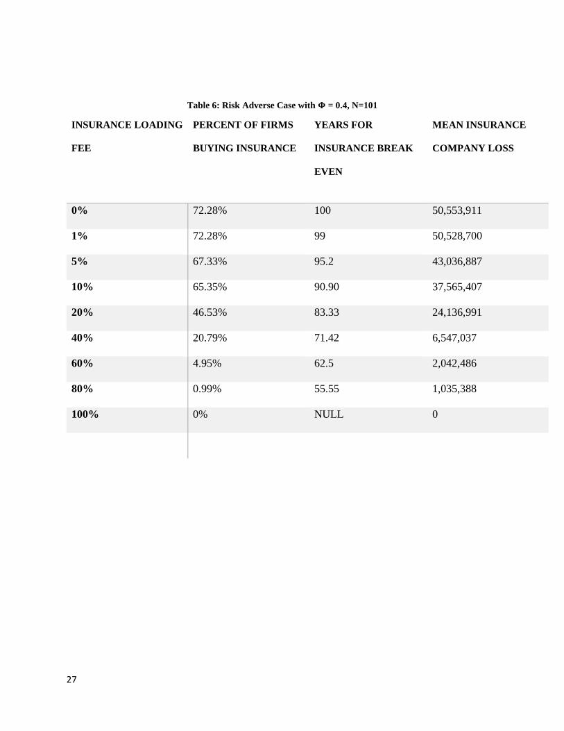
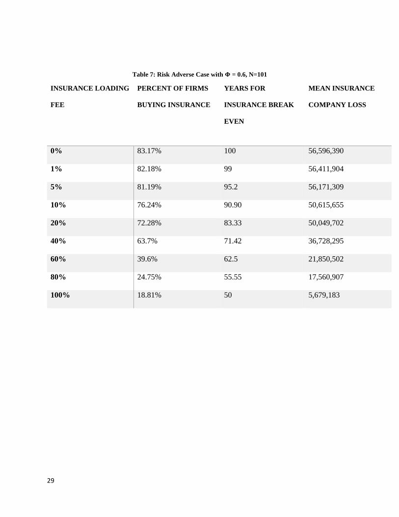
When Φ = 0.4, loading premiums higher than 40% result in a huge majority of the firm

owners no longer finding the contract worthwhile. These results are reported in Table 6, and Plot

1 specifically shows the effect of the loading fee on firms buying insurance. With Φ = 0.6, this

does not occur until 80%, which is an incredibly large loading premium. The results for the

higher value of risk aversion are reported in Table 7 and Plot 2. The lower risk aversion

coefficient seems to reflect expected real world behavior better than the slightly higher

assumption. The insurance company will only earn a profit if a pandemic does not occur until

after the break even point. However, the loss that does result from a pandemic occurring is so

extreme that the mean loss is always negative, even with incredibly high loading fees. The

market is unwilling to bear the loading fees that would result in the insurance company making a

profit on average.

27

Table 6: Risk Adverse Case with 𝚽 = 0.4, N=101

INSURANCE LOADING

FEE

PERCENT OF FIRMS

BUYING INSURANCE

YEARS FOR

INSURANCE BREAK

EVEN

MEAN INSURANCE

COMPANY LOSS

0% 72.28% 100 50,553,911

1% 72.28% 99 50,528,700

5% 67.33% 95.2 43,036,887

10% 65.35% 90.90 37,565,407

20% 46.53% 83.33 24,136,991

40% 20.79% 71.42 6,547,037

60% 4.95% 62.5 2,042,486

80% 0.99% 55.55 1,035,388

100% 0% NULL 0

28

Plot 1: Risk Adverse Case with 𝚽 = 0.4, N=101

0.00%

10.00%

20.00%

30.00%

40.00%

50.00%

60.00%

70.00%

80.00%

0% 20% 40% 60% 80% 100% 120%

Per

cen

t Fi

rms

Bu

yin

g In

sura

nce

Loading Fee

LOADING FEE EFFECT ON FIRMS BUYING INSURANCE

29

Table 7: Risk Adverse Case with 𝚽 = 0.6, N=101

INSURANCE LOADING

FEE

PERCENT OF FIRMS

BUYING INSURANCE

YEARS FOR

INSURANCE BREAK

EVEN

MEAN INSURANCE

COMPANY LOSS

0% 83.17% 100 56,596,390

1% 82.18% 99 56,411,904

5% 81.19% 95.2 56,171,309

10% 76.24% 90.90 50,615,655

20% 72.28% 83.33 50,049,702

40% 63.7% 71.42 36,728,295

60% 39.6% 62.5 21,850,502

80% 24.75% 55.55 17,560,907

100% 18.81% 50 5,679,183

30

Plot 2: Risk Adverse Case with 𝚽 = 0.6, N=101

0.00%

10.00%

20.00%

30.00%

40.00%

50.00%

60.00%

70.00%

80.00%

90.00%

0% 20% 40% 60% 80% 100% 120%

Per

cen

t Fi

rms

Bu

yin

g In

sura

nce

Loading Fee

LOADING FEE EFFECT ON FIRMS BUYING INSURANCE

31

V. Simulation Parameter Sensitivity Analysis

In this section, I test the sensitivity of the baseline results to different parameter

assumptions. To test this, the model will be rerun with Φ = 0.4 and some different assumptions

than the initial results. First, without a correlation between the revenue and expense effect

coefficient distributions. Then, with a different distribution of small businesses in the sample.

Finally, the chance of a pandemic occurring will be altered. Φ = 0.6 will not be considered in the

sensitivity analysis as the lower value was found to better model expected firm behavior in

response to rising costs of insurance.

A. Uncorrelated Case

I begin by removing the correlation between the revenue and expenses effect

distributions. While this assumption does make intuitive sense, I expect that the fundamental

results will not change when running the model without it. Furthermore, if the results persist with

the correlation factor being set to zero, it rules out any potential bias from this assumption that is

solely driving the results. As displayed in Table 8, for the risk neutral case the results are

identical, when the expected value of the contract is zero all risk neutral business owners buy the

insurance, but as soon as even a 1% loading fee is added to the contract and the expected value

becomes negative, none of them are willing to accept the contract. With the risk adverse case for

Φ = 0.4, the results are mostly the same but the effect of loading fee on the number of firms

buying insurance is more pronounced. In the uncorrelated case, the market only tolerates up to a

60% loading fee, whereas in the correlated case this reached as high as 100% with a small

number of firms still purchasing insurance.

32

Table 8: Risk Neutral Case with 𝚽 = 0, N=101, Uncorrelated Effect Coefficients

INSURANCE

LOADING FEE

PERCENT OF FIRMS

BUYING INSURANCE

YEARS FOR

INSURANCE BREAK

EVEN

MEAN INSURANCE

COMPANY LOSS

0% 100% 100 69,955,122

1% 0% NULL 0

Table 9: Risk Adverse Case with 𝚽 = 0.4, N=101

INSURANCE

LOADING FEE

PERCENT OF FIRMS

BUYING INSURANCE

YEARS FOR

INSURANCE BREAK

EVEN

MEAN INSURANCE

COMPANY LOSS

0% 71.29% 100 44,054,835

1% 67.33% 99 43,669,212

5% 63.37% 95.2 40,094,996

10% 58.42% 90.90 36,547,079

20% 41.58% 83.33 30,472,806

40% 18.81% 71.42 6,181,681

60% 3.96 62.5 283,393

80% 0% NULL 0

100% 0% NULL 0

33

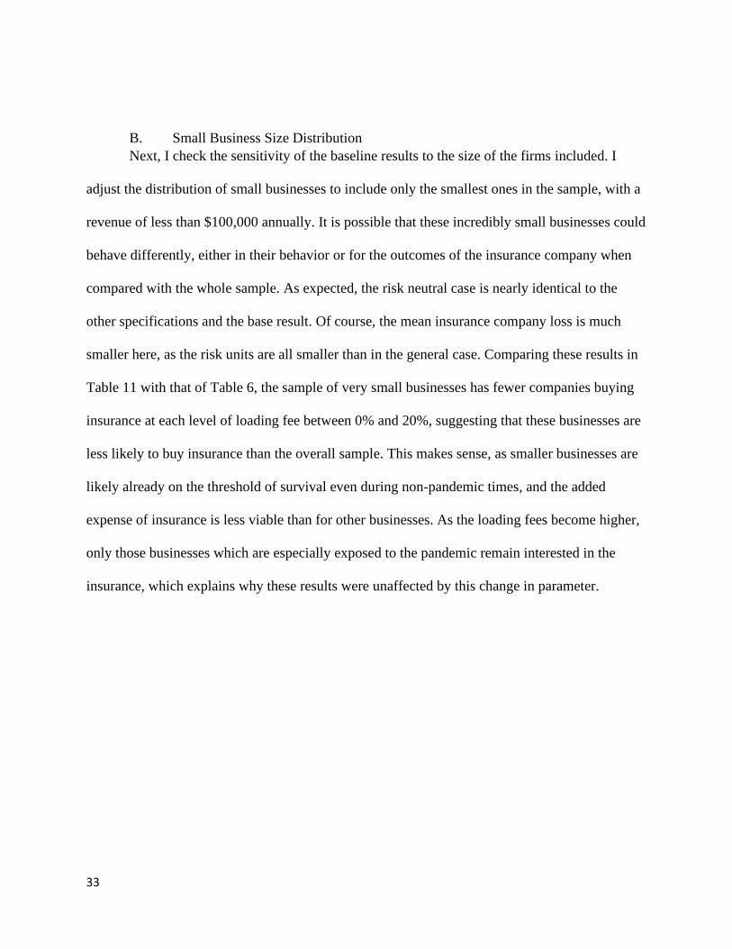
B. Small Business Size Distribution

Next, I check the sensitivity of the baseline results to the size of the firms included. I

adjust the distribution of small businesses to include only the smallest ones in the sample, with a

revenue of less than $100,000 annually. It is possible that these incredibly small businesses could

behave differently, either in their behavior or for the outcomes of the insurance company when

compared with the whole sample. As expected, the risk neutral case is nearly identical to the

other specifications and the base result. Of course, the mean insurance company loss is much

smaller here, as the risk units are all smaller than in the general case. Comparing these results in

Table 11 with that of Table 6, the sample of very small businesses has fewer companies buying

insurance at each level of loading fee between 0% and 20%, suggesting that these businesses are

less likely to buy insurance than the overall sample. This makes sense, as smaller businesses are

likely already on the threshold of survival even during non-pandemic times, and the added

expense of insurance is less viable than for other businesses. As the loading fees become higher,

only those businesses which are especially exposed to the pandemic remain interested in the

insurance, which explains why these results were unaffected by this change in parameter.

34

Table 10: Risk Neutral Case with 𝚽 = 0, N=101, Revenue < 100k

INSURANCE

LOADING FEE

PERCENT OF FIRMS

BUYING INSURANCE

YEARS FOR

INSURANCE BREAK

EVEN

MEAN INSURANCE

COMPANY LOSS

0% 100% 100 6,546,352

1% 0% NULL 0

Table 11: Risk Adverse Case with 𝚽 = 0.4, N=101

INSURANCE LOADING

FEE

PERCENT OF FIRMS

BUYING INSURANCE

YEARS FOR

INSURANCE BREAK

EVEN

MEAN INSURANCE

COMPANY LOSS

0% 71.84% 100 6,263,936

1% 67.96% 99 6,191,901

5% 63.11% 95.2 6,093,324

10% 57.28% 90.90 5,981,106

20% 41.75% 83.33 5,660,180

40% 21.36% 71.42 6,181,681

60% 6.8% 62.5 3,541,985

80% 0% NULL 0

100% 0% NULL 0

35

C. Pandemic Chance

As the world population grows, and in absolute value the number of people in poor living

conditions increases, the chances of a pandemic occurring are likely to increase (Dodds, 2019).

Therefore, this sensitivity analysis will consider the impact of assuming a 2% chance of a

pandemic occurring instead of a 1% chance. This adjustment is made to reflect the unfortunate

reality that the previous estimate may not be accurate in the future, and that pandemics will

become more likely. Once more, as expected, the risk neutral case presented in Table 12 shows

no fluctuation and risk neutral business owners continue to decline contracts of negative

expected value. In the risk averse case, with results presented in the table 13, I find the results to

be completely identical. This does not make the most intuitive sense, as ceteris paribus the more

likely an adverse event is, the more businesses that should want to be insured against it. This is

probably a result of the way the simulation is designed, with both the insurance company and the

small business owners assumed to have perfect information of the exact impact of the pandemic

on the firm, as well as the exact probablity. In a real-world setting, both of these are not known

variables and instead have to be estimated.

36

Table 12: Risk Neutral Case with 𝚽 = 0, N=101, Pandemic Chance = 2%

INSURANCE LOADING

FEE

PERCENT OF FIRMS

BUYING INSURANCE

YEARS FOR

INSURANCE BREAK

EVEN

MEAN INSURANCE

COMPANY LOSS

0% 100% 100 63,007,685

1% 0% NULL 0

Table 13: Risk Adverse Case with 𝚽 = 0.4, N=101, Pandemic Chance = 2%

INSURANCE

LOADING FEE

PERCENT OF FIRMS

BUYING INSURANCE

YEARS FOR

INSURANCE BREAK

EVEN

MEAN INSURANCE

COMPANY LOSS

0% 72.28% 100 48,032,869

1% 72.28% 99 47,982,448

5% 67.33% 95.2 43,036,887

10% 65.35% 90.90 37,565,407

20% 46.53% 83.33 24,136,991

40% 20.79% 71.42 6,547,037

60% 4.95% 62.5 2,042,486

80% 0.99% 55.55 1,035,388

100% 0% NULL 0

37

VI. Conclusion I explored the viability of business interruption insurance covering pandemic risk using

simulations. The simulation model made assumptions about the probability, the feasibility of

the premiums, and the loss's magnitude. It is likely an insurance company attempting to

insurance a pandemic would make errors when attempting to estimate a probability of loss

and the magnitude of the loss. These were taken as given by the insurance company in the

simulation. Despite simulation conditions being more favorable for the insurance company

than real-world conditions, in no estimation of the model did the insurance company turn a

profit. This thesis's primary result is strong: It is abundantly clear, both by theory and

simulation, that pandemics represent a catastrophic event that is utterly uninsurable in the

traditional insurance model. This result persisted among several differing robustness checks

on the simulation parameters.

This research was limited by the lack of available base small business data, instead

having to relying on assumptions for simulation. Doing the analysis on actual small business

data, and only having the insurance product being simulated would have been clearly

preferable. These assumptions were also made based strictly on the COVID-19 pandemic, so

generalizing to all pandemics should be done with care. Additionally, the utility function

selected does capture most of the intuition but does result in a contradiction when it implies

that risk neutral business owners will buy insurance more often than risk averse ones when

the insurance is actuarially fair. However, the average return of the insurance company

would still be negative, as it was in the risk neutral case.

38

The model was also unable to capture a potential source of moral hazard in the insurance

contracts as described. Business owners have a significant amount of control over the type of

services they offer and the amount of time they are open. If the contracts are structured to

completely recoup lost revenue, there is a strong perverse incentive for firms to sharply

curtail hours worked, as the insurance company would be obligated to foot the bill. Insurance

companies may have to require a minimum number of open hours or place an upper limit on

the amount they will pay out. Another approach is to not offer full coverage, and instead

require the business owner be responsible for some of the loss. The incentive to cut services

is not nearly as strong when the businessowners themselves are on the hook for some of the

lost revenue.

Further research is needed to determine the most viable alternative solution, which will

almost assuredly involve the government in some capacity. This public-private partnership

could take a variety of forms. For example, the government could act as reinsurer and charge

the insurance company a percentage of their profit to take on the risk beyond a certain

amount of loss. The government is likely to have to respond to the pandemic in the first place

and having a system setup already through this insurance scheme could increase the speed at

which funds can be distributed to business owners. Another option is for the insurance

company to structure this product as a loan, where firms will pay back the coverage received

in exchange for a lower premium. This solution would involve the government twice, to

ensure there are adequate funds when the catastrophic loss hits, and to make sure that

businesses do not default on their loan during the course of repayment. Additional research

39

should be done, and an appropriate system put in place before the next pandemic hits small

businesses and wreaks the same havoc that COVID-19 has.

40

R Code For Simulation

41

VII. Appendix #function that takes simulation parameters and then runs simulation)

simulation <- function(SampleSize, RiskAversion, LoadingFee, PandemicChance){

#converts loading fee to percentage for output purposes

ins_loading_fee_report <- (ins_loading_fee-1)*100

#divides annual chance of pandemic among the months

ins_monthly_pandemic_chance <- ins_yearly_pandemic_chance/12

#generation of annual business revenue data, percentages found in table 1

sb_rev_less_100k <- rnorm(n=.20*ss, mean = 50000, sd = 20000)

sb_rev_less_1mm <- rnorm(n=.51*ss, mean = 500000, sd = 200000)

sb_rev_less_10mm <- rnorm(n=.26*ss, mean = 5000000, sd = 2000000)

sb_rev_more_10mm <- rnorm(n=.04*ss, mean = 13000000, sd = 2000000)

sb_rev <- c(sb_rev_less_100k, sb_rev_less_1mm, sb_rev_less_10mm, sb_rev_more_10mm)

#adjusting sample size for the slight inflation that occurs

ss <- length(sb_rev)

#generation of phased based revenue effects

#loading package to create correlated variables

library(fabricatr)

rho_value <- 0.8

sb_rev_ld_effect <- rnorm(n=ss, mean = -0.6, sd = .1)

sb_rev_sd_effect <- correlate(given = sb_rev_ld_effect, rho = rho_value, rnorm, mean=-0.25, sd = .1)

#generation of profit margin data

42

sb_pm <- rnorm(n=ss, mean = 0.07, sd = 0.03)

#generation of dataframe with aggerated data

sb_df <- data.frame(RevAn=sb_rev, RevEffectLD = sb_rev_ld_effect, RevEffectSD = sb_rev_sd_effect,

PM = sb_pm )

#monthly revenue data

sb_df$RevMonthly <- sb_df$RevAn/12

#pre pandemic expenses

sb_df$ExpMonthly <- -sb_df$PM*sb_df$RevMonthly+sb_df$RevMonthly

#pre pandemic profit

sb_df$ProfitMonthly <- sb_df$RevMonthly-sb_df$Exp

#generation of phased based expense effects

sb_lockdown_phase_exp <- rnorm(n=ss, mean=-.6, sd=.1)

sb_df$ExpEffectLD <- sb_lockdown_phase_exp

sb_socialdist_phase_exp <- correlate(given = sb_lockdown_phase_exp, rho = rho_value, rnorm, mean=-

.2, sd = .1)

sb_df$ExpEffectSD <- sb_socialdist_phase_exp

#lock down revenue

sb_df$RevMonthlyLD <- 0

#looping over the rows to calculate the monthly post pandemic revenue, the sign of the $RevEffectLD

column indicates if the firm is a gaining or losing type

#in either case, simply adding the value found from multiplying the monthly revenue by the percent

change yields the adjusted revenue

for (i in 1:dim(sb_df)[1]) {

43

sb_df$RevMonthlyLD[i] <- sb_df$RevMonthly[i]+(sb_df$RevMonthly[i]*sb_df$RevEffectLD[i])

}

#lockdown expenses

for (i in 1:dim(sb_df)[1]) {

sb_df$ExpMonthlyLD[i] <- sb_df$ExpMonthly[i]+(sb_df$ExpEffectLD[i]*sb_df$ExpEffectLD[i])

}

#lockdown profit

sb_df$ProfitMonthlyLD <- sb_df$RevMonthlyLD-sb_df$ExpMonthlyLD

#social distancing revenue

sb_df$RevMonthlySD <- 0

for (i in 1:dim(sb_df)[1]) {

sb_df$RevMonthlySD[i] <- sb_df$RevMonthly[i]+(sb_df$RevMonthly[i]*sb_df$RevEffectSD[i])

}

#social distancing expenses

for (i in 1:dim(sb_df)[1]) {

sb_df$ExpMonthlySD[i] <- sb_df$ExpMonthly[i]+(sb_df$ExpEffectSD[i]*sb_df$ExpEffectSD[i])

}

#total lost/gained revenue

sb_df$RevEffectTotal <- -1*((sb_df$RevMonthly*21)-

((sb_df$RevMonthlyLD*3)+(sb_df$RevMonthlySD*18)))

sb_df$RevEffectMonthly <- sb_df$RevEffectTotal/21

44

#lockdown profit

sb_df$ProfitMonthlyLD <- sb_df$RevMonthlyLD-sb_df$ExpMonthlyLD

#social distancing profit

sb_df$ProfitMonthlySD <- sb_df$RevMonthlySD-sb_df$ExpMonthlySD

#total profit

sb_df$ProfitEffectTotal <- -1*((sb_df$ProfitMonthly*21)-

((sb_df$ProfitMonthlyLD*3)+(sb_df$ProfitMonthlySD*18)))

sb_df$ProfitEffectMonthly <- sb_df$ProfitEffectTotal/21

#building insurance company dataframe

ins_payout_total <- -1*sb_df$RevEffectTotal

ins_df <- data.frame(PayoutTotal = ins_payout_total)

ins_df$PayoutTotal <- ins_df$PayoutTotal

ins_df$MonthlyPayout <- ins_df$PayoutTotal/21

ins_df$MonthlyPremiums <- (ins_df$MonthlyPayout*ins_monthly_pandemic_chance)*ins_loading_fee

#building dataframe of effect of having/not having insurance in the pandemic and not having pandemic

cases

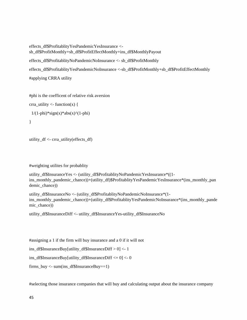
effects_df <- data.frame(ProfitablityNoPandemicYesInsurance = sb_df$ProfitMonthly-

ins_df$MonthlyPremiums)

45

effects_df$ProfitablityYesPandemicYesInsurance <-

sb_df$ProfitMonthly+sb_df$ProfitEffectMonthly+ins_df$MonthlyPayout

effects_df$ProfitablityNoPandemicNoInsurance <- sb_df$ProfitMonthly

effects_df$ProfitablityYesPandemicNoInsurance <-sb_df$ProfitMonthly+sb_df$ProfitEffectMonthly

#applying CRRA utility

#phi is the coefficent of relative risk aversion

crra_utility <- function(x) {

1/(1-phi)*sign(x)*abs(x)^(1-phi)

}

utility_df <- crra_utility(effects_df)

#weighting utilites for probablity

utility_df$InsuranceYes <- (utility_df$ProfitablityNoPandemicYesInsurance*((1-

ins_monthly_pandemic_chance))+(utility_df)$ProfitablityYesPandemicYesInsurance*(ins_monthly_pan

demic_chance))

utility_df$InsuranceNo <- (utility_df$ProfitablityNoPandemicNoInsurance*(1-

ins_monthly_pandemic_chance))+(utility_df$ProfitablityYesPandemicNoInsurance*(ins_monthly_pande

mic_chance))

utility_df$InsuranceDiff <- utility_df$InsuranceYes-utility_df$InsuranceNo

#assigning a 1 if the firm will buy insurance and a 0 if it will not

ins_df$InsuranceBuy[utility_df$InsuranceDiff > 0] <- 1

ins_df$InsuranceBuy[utility_df$InsuranceDiff <= 0] <- 0

firms_buy <- sum(ins_df$InsuranceBuy==1)

#selecting those insurance companies that will buy and calculating output about the insurance company

46

ins_df <- subset(ins_df, subset=(InsuranceBuy==1))

ins_payout_total <- sum(ins_df$PayoutTotal)

ins_prem <- sum(ins_df$MonthlyPremiums)

ins_years_break_even <- (ins_payout_total/ins_prem)/(21*12)

ins_expected_return <- 0

#monte carlo simulation of the insurance companies returns

pandemic_sim <- function(years){

pandemic <- rbinom(years, 1, 0.01)

index <- match(1, pandemic)

index[is.na(index)] <- 0

if (index > 0) {

ins_expected_return <- (index*12*ins_prem)-ins_payout_total

} else {

ins_expected_return <- years*12*ins_prem

}

return(ins_expected_return)

}

runs <- 100000

years <- 100

ins_final_returns <- (replicate(runs,pandemic_sim(years)))

ins_profitable <- (sum(ins_final_returns > 0)/runs)*100

ins_mean_return <- mean(ins_final_returns)

ins_median_return <-median(ins_final_returns)

#reports output of the simulation

output <- function() {

cat(firms_buy, "firms", "out of", ss, "will buy insurance assuming their owners' max utility under

CRRA", "with risk aversion factor of", phi, "and insurance loading fee of", ins_loading_fee_report, "%" )

47

cat("\n")

percent_firms <- round((firms_buy/ss)*100, 2)

cat(percent_firms, "% of the firms will buy insurance")

cat("\n")

cat("The insurance company must collect premiums for", ins_years_break_even, "years without a

pandemic occurring to at least break even. ")

cat("This will occur", round(ins_profitable,2), "% of the time. ")

cat("The mean return of the insurance company is", ins_mean_return, "and the median return is",

ins_median_return)

}

output()

}

#initial sample size parameter

#the final sample size will be slightly larger due to the percentages for rev dist not added to 100% due to

rounding in the source data

ss <- 100

#setting seed

set.seed(1337)

#variable parameters

phi <- 0

ins_loading_fee <- 1.0

ins_yearly_pandemic_chance <- 0.01

#calling the simulation funciton with given parameters

simulation(ss,phi,ins_loading_fee,ins_yearly_pandemic_chance)

48

VIII. References Adiel, Ron. 1996. “Reinsurance and the Management of Regulatory Ratios and Taxes in the

Property—Casualty Insurance Industry.” Journal of Accounting and Economics, Conference

Issue on Contemporary Financial Reporting Issues, 22 (1): 207–40.

https://doi.org/10.1016/S0165-4101(96)00436-3.

Baker, Scott R, Nicholas Bloom, Steven J Davis, Kyle Kost, Marco Sammon, and Tasaneeya

Viratyosin. 2020. “The Unprecedented Stock Market Reaction to COVID-19.” The Review of

Asset Pricing Studies, July, raaa008. https://doi.org/10.1093/rapstu/raaa008.

Barseghyan, Levon, Francesca Molinari, Ted O’Donoghue, and Joshua C. Teitelbaum. 2018.

“Estimating Risk Preferences in the Field.” Journal of Economic Literature 56 (2): 501–64.

https://doi.org/10.1257/jel.20161148.

Bartik, Alexander W., Marianne Bertrand, Zoe Cullen, Edward L. Glaeser, Michael Luca, and

Christopher Stanton. 2020. “The Impact of COVID-19 on Small Business Outcomes and

Expectations.” Proceedings of the National Academy of Sciences 117 (30): 17656–66.

https://doi.org/10.1073/pnas.2006991117.

Bhattacharya, Jay, Peter Tu, and Timothy Hyde. 2013. Health Economics.

Charumilind, Sarun, Matt Craven, Jessica Lamb, Adam Sabow, and Matt Wilson. n.d. “When Will the

COVID-19 Pandemic End? | McKinsey.” Accessed February 22, 2021.

https://www.mckinsey.com/industries/healthcare-systems-and-services/our-insights/when-will-

the-covid-19-pandemic-end.

Chetty, Raj, John Friedman, Nathaniel Hendren, Michael Stepner, and The Opportunity Insights

Team. 2020. “The Economic Impacts of COVID-19: Evidence from a New Public Database

Built Using Private Sector Data.” w27431. Cambridge, MA: National Bureau of Economic

Research. https://doi.org/10.3386/w27431.

Cutler, David M, and Richard J Zeckhauser. 1997. “Reinsurance for Catastrophes and Cataclysms.”

Working Paper 5913. Working Paper Series. National Bureau of Economic Research.

https://doi.org/10.3386/w5913.

Dodds, Walter. 2019. “Disease Now and Potential Future Pandemics.” The World’s Worst Problems,

December, 31–44. https://doi.org/10.1007/978-3-030-30410-2_4.

Edesess, Michael. 2015. “Catastrophe Bonds: An Important New Financial Instrument.” Alternative

Investment Analyst Review, 6.

Federal Reserve. 2019. “Survey & Reports.” 2019. https://www.fedsmallbusiness.org/survey.

Government of Canada, Innovation. 2015. “SME Operating Performance - SME Research and

Statistics.” Reports;Related Links. Innovation, Science and Economic Development Canada.

April 20, 2015. https://www.ic.gc.ca/eic/site/061.nsf/eng/h_02941.html#toc-03.01.

49

Henebry, Kathleen L., and George E. Rejda. 1995. Principles of Risk Management and Insurance.

Vol. 62. https://www.jstor.org/stable/253600?origin=crossref.

Hofmann, Annette, and David Pooser. 2017. “Insurance-Linked Securities: Structured and Market

Solutions.” In The Palgrave Handbook of Unconventional Risk Transfer, edited by Maurizio

Pompella and Nicos A Scordis, 357–73. Cham: Springer International Publishing.

https://doi.org/10.1007/978-3-319-59297-8_12.

Homebase. n.d. “Coronavirus Stats: Impact on Local Small Business.” Homebase. Accessed February

8, 2021. https://joinhomebase.com/data/.

Karaca-Mandic, Pinar, et al. “How Do Health Insurance Loading Fees Vary by Group Size?: Implications

for Healthcare Reform.” International Journal of Health Care Finance and Economics, vol. 11, no. 3,

2011, pp. 181–207. JSTOR, www.jstor.org/stable/23280301. Accessed 14 Apr. 2021.

https://www.jstor.org/stable/23280301

Klein, Robert W. 2014. “A Primer on The Economics of Insurance.”

https://doi.org/10.13140/2.1.4487.9681.

Madhav, Nita, Ben Oppenheim, Mark Gallivan, Prime Mulembakani, Edward Rubin, and Nathan

Wolfe. 2017. “Pandemics: Risks, Impacts, and Mitigation.” In Disease Control Priorities:

Improving Health and Reducing Poverty, edited by Dean T. Jamison, Hellen Gelband, Susan

Horton, Prabhat Jha, Ramanan Laxminarayan, Charles N. Mock, and Rachel Nugent, 3rd ed.

Washington (DC): The International Bank for Reconstruction and Development / The World

Bank. http://www.ncbi.nlm.nih.gov/books/NBK525302/.

Polacek, Andy. 2018. “Catastrophe Bonds: A Primer and Retrospective.” Chicago Fed Letter.

https://doi.org/10.21033/cfl-2018-405.

“Pool Re.” 2019. Pool Reinsurance Company LTD. 2019. https://www.poolre.co.uk/.

Ramnath, Shanti. 2020. “What Is Business Interruption Insurance and How Is It Related to the Covid-

19 Pandemic?” Chicago Fed Letter. https://doi.org/10.21033/cfl-2020-440.

Rothschild, Michael, and Joseph Stiglitz. 1976. “Equilibrium in Competitive Insurance Markets: An

Essay on the Economics of Imperfect Information.” The Quarterly Journal of Economics 90 (4):

629. https://doi.org/10.2307/1885326.

U.S. Bureau of Economic Analysis (BEA). n.d. “Gross Domestic Product, 2nd Quarter 2020

(Advance Estimate) and Annual Update.” Accessed November 11, 2020.

https://www.bea.gov/news/2020/gross-domestic-product-2nd-quarter-2020-advance-estimate-

and-annual-update.

50

World Bank. n.d. “Fact Sheet: Pandemic Emergency Financing Facility.” World Bank. Accessed

August 25, 2020. https://www.worldbank.org/en/topic/pandemics/brief/fact-sheet-pandemic-

emergency-financing-facility.

“World Bank Abandons Pandemic Bond Instrument after Disastrous Covid-19 Response.” 2020.

Bretton Woods Project. October 6, 2020. https://www.brettonwoodsproject.org/2020/10/world-

bank-abandons-pandemic-bond-instrument-after-disastrous-covid-19-response/.