Simulation of line fault locator on HVDC Light electrode line344138/FULLTEXT01.pdf · BACHELOR’S...

BACHELOR’S THESIS Electrical Engineering, Electric Power Technology Department of Engineering Science

August 10, 2010

Simulation of line fault locator on HVDC Light electrode line Andreas Hermansson

BACHELOR’S THESIS

i

Simulation of line fault locator on HVDC Light elec trode line

Summary

In this bachelor thesis, cable fault locators are studied for use on the overhead electrode

lines in the HVDC (High Voltage Direct Current) Light project Caprivi Link.

The cable fault locators studied operates with the principle of travelling waves, where a

pulse is sent in the tested conductor. The time difference is measured from the injection

moment to the reflection is received. If the propagation speed of the pulse is known the

distance to the fault can be calculated. This type of unit is typically referred to as a TDR

(Time Domain Reflectometer). The study is performed as a computer simulation where a

simplified model of a TDR unit is created and applied to an electrode line model by using

PSCAD/EMTDC. Staged faults of open circuit and ground fault types are placed at three

distances on the electrode line model, different parameters of the TDR units such as pulse

width and pulse amplitude along with its connection to the electrode line are then studied

and evaluated.

The results of the simulations show that it is possible to detect faults of both open circuit

and ground fault types with a suitable TDR unit. Ground faults with high resistance

occurring at long distances can be hard to detect due to low reflection amplitudes from the

injections. This problem can somewhat be resolved with a function that lets the user

compare an old trace of a “healthy” line with the new trace. The study shows that most of

the faults can be detected and a distance to the fault can be calculated within an accuracy of

± 250 m.

The pulse width of the TDR needs to be at least 10 µs, preferable 20 µs to deliver high

enough energy to the fault to create a detectable reflection. The pulse amplitude seams to

be of less significance in this simulation, although higher pulse amplitude is likely to be

more suitable in a real measurement due to the higher energy delivered to the fault. The

Hipotronics TDR 1150 is a unit that fulfil these requirements and should therefore be able

to work as a line fault locator on the electrode line.

Date: August 10, 2010 Author : Andreas Hermansson Examiner : Lars Holmblad Advisor : Sören Nyberg, ABB AB Programme : Electrical Engineering, Electric Power Technology Main field of study : Electrical Engineering Education level : Bachelor Credits : 15 HE credits Keywords Line fault locator, TDR, Arc reflection, simulation, electrode line, HVDC Publisher : University West, Department of Engineering Science,

S-461 86 Trollhättan, SWEDEN Phone: + 46 520 22 30 00 Fax: + 46 520 22 32 99 Web: www.hv.se

Simulation of line fault locator on HVDC Light electrode line

ii

Preface

I would like to thank Anna-Karin Skytt and Sören Nyberg at ABB AB who made this

bachelor’s thesis possible.

Andreas Hermansson

Ludvika 9 April 2010


iii

Contents Summary .............................................................................................................................................. i Preface ................................................................................................................................................ ii Abbreviations ................................................................................................................................... iv 1 Introduction ................................................................................................................................ 1

1.1 Background ....................................................................................................................... 1 1.2 Project description ........................................................................................................... 2 1.3 Methodology ..................................................................................................................... 2

2 Theory .......................................................................................................................................... 4 2.1 Travelling waves ............................................................................................................... 4 2.2 Description of the time domain reflectometer (TDR) ............................................... 6 2.3 Description of the impulse thumper ............................................................................. 6 2.4 Description of the arc reflection method ..................................................................... 7

3 Design .......................................................................................................................................... 8 3.1 Modelling of electrode line ............................................................................................. 8 3.2 Modelling of line fault locator ...................................................................................... 10

3.2.1 Time domain reflectometer ............................................................................ 10 3.2.2 Arc reflection .................................................................................................... 11

3.3 Fault model ..................................................................................................................... 12 4 Simulations ................................................................................................................................ 13

4.1 Fault type ......................................................................................................................... 13 4.1.1 Low resistance to ground ................................................................................ 14 4.1.2 High resistance to ground ............................................................................... 15 4.1.3 Open circuit ...................................................................................................... 16

4.2 Pulse width ...................................................................................................................... 17 4.3 Pulse amplitude .............................................................................................................. 18 4.4 Connection ...................................................................................................................... 19 4.5 Parallel/single line .......................................................................................................... 21 4.6 Electrode station configuration ................................................................................... 22 4.7 Arc reflection .................................................................................................................. 24

5 Results and analysis .................................................................................................................. 26 5.1 Fault type ......................................................................................................................... 26

5.1.1 Low resistance ground fault ............................................................................ 26 5.1.2 High resistance ground fault ........................................................................... 27 5.1.3 Open circuit ...................................................................................................... 28

5.2 Pulse width ...................................................................................................................... 28 5.3 Pulse amplitude .............................................................................................................. 29 5.4 Connection ...................................................................................................................... 29 5.5 Parallel/single line .......................................................................................................... 30 5.6 Electrode station configuration ................................................................................... 31 5.7 Arc reflection .................................................................................................................. 31

6 Conclusions and future work ................................................................................................. 33 References ........................................................................................................................................ 34


iv

Abbreviations

HVDC High Voltage Direct Current

IGBT Insulated Gate Bipolar Transistor

LFL Line Fault Locator

TDR Time Domain Reflectometer


1

1 Introduction

1.1 Background

Caprivi Link is a HVDC Light project that will be delivered to Namibia during 2010.

HVDC Light is a power transmission system developed by ABB that is based on voltages

source converters using IGBT semiconductors and high frequency pulse width modulation

to convert from AC to DC and back again. The Light version is available in the range from

50 to 1200 MW [1].

The project consists of converter stations, in Zambezi and Gerus, connected by two

overhead lines approximately 970 km long. The link has a power rating of 300 MW

operating at a DC voltage of 350 kV. This is the first HVDC Light project to be built with

overhead lines. At a first stage one monopole is delivered but there is an option to expand

to a bipole. This transmission link is very important for the power supply of the country as

the networks in the region are very weak [2].

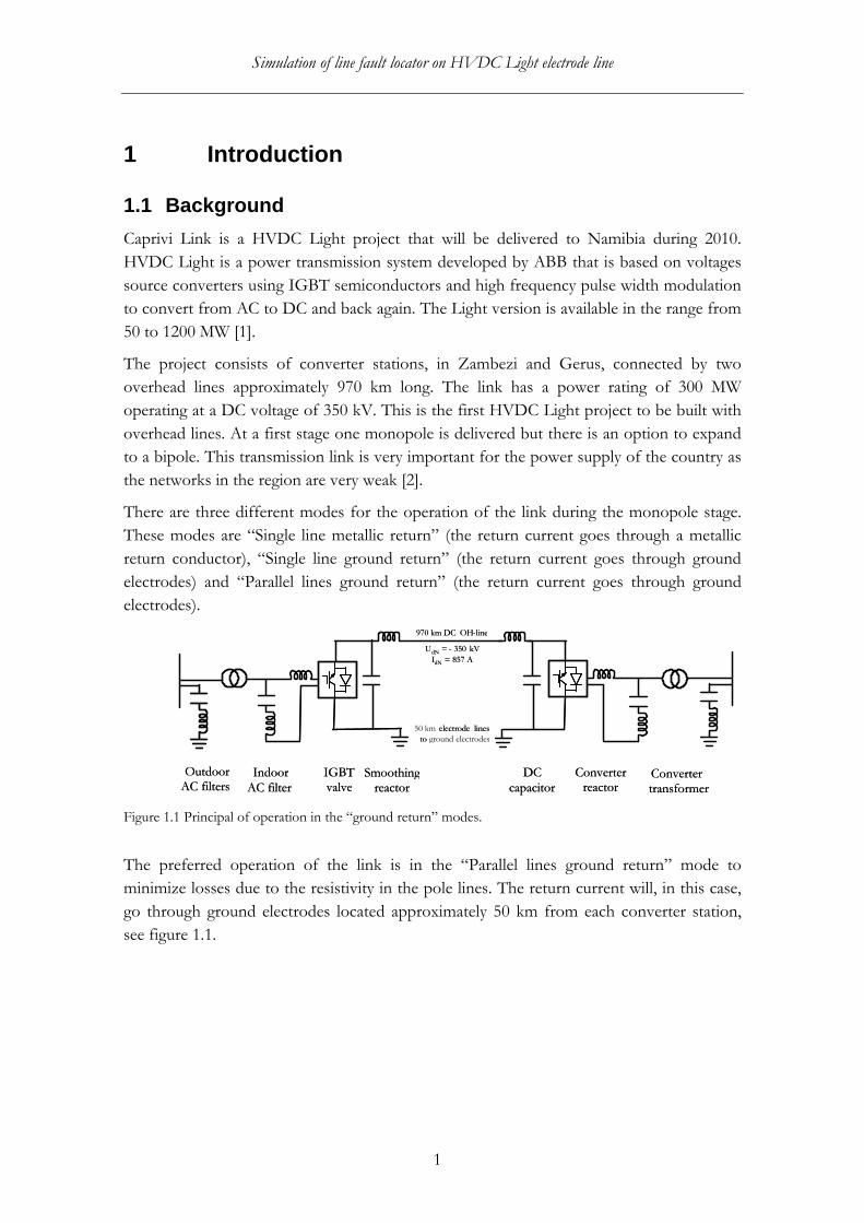
There are three different modes for the operation of the link during the monopole stage.

These modes are “Single line metallic return” (the return current goes through a metallic

return conductor), “Single line ground return” (the return current goes through ground

electrodes) and “Parallel lines ground return” (the return current goes through ground

electrodes).

Figure 1.1 Principal of operation in the “ground return” modes.

The preferred operation of the link is in the “Parallel lines ground return” mode to

minimize losses due to the resistivity in the pole lines. The return current will, in this case,

go through ground electrodes located approximately 50 km from each converter station,

see figure 1.1.

OutdoorAC filters

IndoorAC filter

IGBTvalve

Converter reactor

Converter transformer

DC capacitor

Smoothingreactor

970 km DC OH-line UdN = - 350 kV

I dN = 857 A

50 km electrode lines

to ground electrodes

OutdoorAC filters

IndoorAC filter

IGBTvalve

Converter reactor

Converter transformer

DC capacitor

Smoothingreactor

970 km DC OH-line UdN = - 350 kV

I dN = 857 A

electrode lines

to


2

1.2 Project description

A fault on the pole line can be detected on-line by detecting the incoming travelling waves

in each station, by comparing the arrival time of waves in the two stations the location can

be determined. However, as the voltage on the electrode lines is approximately zero or very

low, this method is not applicable.

The aim of this study is to find equipment that can detect the location of the fault along the

electrode line.

It can be off-line equipment, i.e. does not need to locate the fault when the link is in

operation. The fault locator will inject a pulse into the line and detect the time when the

reflected pulse comes back.

The simulations should answer a number of issues which affect the ability to locate a fault.

How different types of faults, distances to faults, pulse amplitude, pulse width affect the

ability to locate a fault. The simulation should also elucidate the existence of any

interference from parallel lines

1.3 Methodology

Since the electrode line is still under construction and a similar overhead line is hard to get

access to for field measurements, the study will be performed as a simulation using

PSCAD/EMTDC.

PSCAD/EMTDC is simulation software for design and verification of power systems.

EMTDC is a simulation engine and PSCAD is a graphical user interface, see figure

1.2. PSCAD/EMTDC is suitable for simulating electromagnetic transients or instantaneous

solutions.

Simplified models of the line fault locators are constructed from manufacturer’s datasheets

and information from their sales representatives. The LFL models are applied to electrode

line models with staged faults. Different parameters are varied one at a time to study the

behaviour of the LFL.


3

Figure 1.2 The PSCAD simulation environment.


4

2 Theory

2.1 Travelling waves

Any electrical charge applied to a conductor, such as a lightning stroke or the closing of a

circuit breaker, causes a rise of the potential of the conductor. This produces travelling

waves of voltage e and current i that propagates along the conductor at the speed of light.

The voltage and current waves are related by a surge impedance Z. For a lossless

transmission line, Z is dependent only to the inductance and capacitance according to

equations (1).

i

eZ =

(1)

C

LZ =

If a voltage and current wave hit a point of discontinuity in the impedance, while

propagating along a conductor, voltage and current waves are reflected backward and

transmitted forward from the point of discontinuity.

I.e. consider two conductors in series with surge impedances Z1 and Z2. Let the original

forward waves be denoted as e and i, the waves reflected backwards from the discontinuity

point be denoted e’ and i’ and the waves transmitted forward be denoted e’’ and i’’. Then

the normal equations (2) describe the travelling wave and the boundary equations (3) the

relationship at the point of discontinuity [3].

Normal equations

''''

''

2

1

1

iZe

iZe

iZe

⋅=⋅=⋅=

(2)

Boundary equations

'''

'''

iii

eee

−=+=

(3)


5

Then in terms of e and i we get

iZZ

Zi

iZZ

ZZi

eZZ

Ze

eZZ

ZZe

21

1

21

12

21

2

21

12

2''

'

2''

'

+⋅

=

⋅+−

=

+⋅

=

⋅+−

=

(4)

Now we can draw the following conclusions from equations (4) about the current and

voltage waves at the point of discontinuity:

If Z1=Z2, the reflected current and voltage waves are zero and the transmitted current and

voltage waves are equal to the original current and voltage waves.

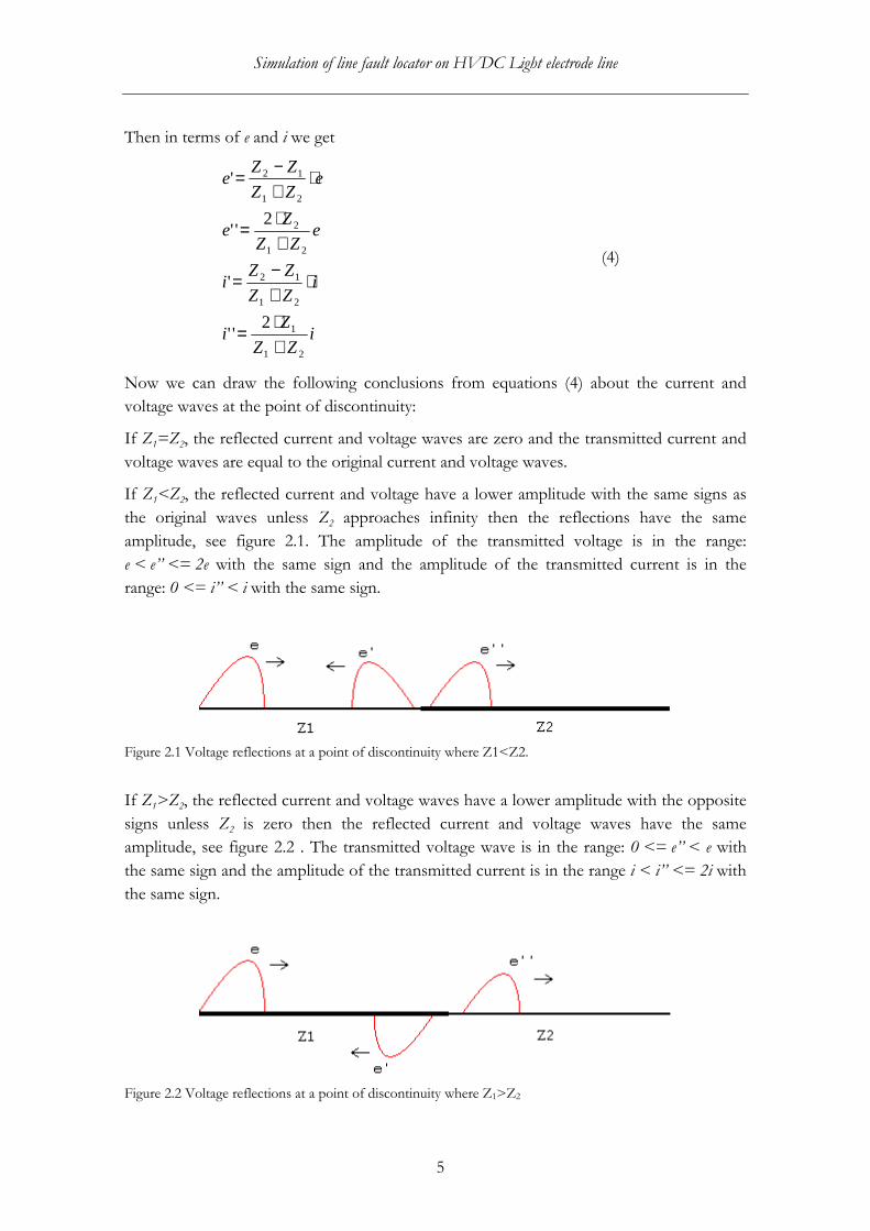
If Z1<Z2, the reflected current and voltage have a lower amplitude with the same signs as

the original waves unless Z2 approaches infinity then the reflections have the same

amplitude, see figure 2.1. The amplitude of the transmitted voltage is in the range:

e < e’’ <= 2e with the same sign and the amplitude of the transmitted current is in the

range: 0 <= i’’ < i with the same sign.

Figure 2.1 Voltage reflections at a point of discontinuity where Z1<Z2.

If Z1>Z2, the reflected current and voltage waves have a lower amplitude with the opposite

signs unless Z2 is zero then the reflected current and voltage waves have the same

amplitude, see figure 2.2 . The transmitted voltage wave is in the range: 0 <= e’’ < e with

the same sign and the amplitude of the transmitted current is in the range i < i’’ <= 2i with

the same sign.

Figure 2.2 Voltage reflections at a point of discontinuity where Z1>Z2


6

2.2 Description of the time domain reflectometer (T DR)

A time domain reflectometer, TDR, or pulse echo meter is a device which can measure

distances to changes in the impedance of a conductor. The technique is based upon the

principle of travelling waves. A short rise time pulse is injected in the conductor and it is

partly reflected by impedance discontinuities in the line. The trace is then displayed on an

oscilloscope screen. By measuring the travel time t between the pulse is sent and a

reflection is received it’s possible to calculate the distance to the discontinuity that caused

the reflection. To calculate the distance to the fault the wave propagation speed vp has to be

known. The wave propagation speed for an overhead transmission line is close to the speed

of light and can be calculated by equation (5) [3], where L is the inductance and C is the

capacitance per unit length. Then the distance d to the fault is given by equation (6). The

wave propagation speed can also be measured with a known length of the line by

extraction from equation (6), this will give the exact propagation speed of the conductor.

LC

v p

1= (5)

2

tvd p ⋅

= (6)

By inspecting the waveform of the reflection it’s possible to determine what type of fault

caused the reflection. From the conclusions in chapter 3.1 a short circuit is represented by

a negative reflection and an open circuit represented of a positive reflection. For a high

resistance shunt fault it’s likely that the amplitude of the reflection is too small to be

detectable. To resolve this problem some TDR units have a storage function so that an old

trace can be compared with a new one, there deviations between the two traces can point

out a fault [4].

2.3 Description of the impulse thumper

An impulse thumper is a high energy capacitive discharge unit that transmit a high energy

pulse between the faulty conductor and ground. The unit basically consists of a power

supply, capacitors and a high voltage switch. When the pulse reaches the fault location it

creates an arc which makes an audible thump. The fault can then be found simply by

listening after the thump created by the arc with a microphone or a magnetic loop antenna,

however this method is not applicable on an overhead line [4].


7

2.4 Description of the arc reflection method

The arc reflection method combines the use of a high capacitive discharge unit and a TDR.

The thumper and the TDR are connected via a filter that protects the TDR from the high

voltage pulses created by the thumper. When the energy pulse reaches a high resistance

fault it creates an arc that lowers the resistance of the fault. Simultaneously the TDR unit

can measure the distance to the arc [4].


8

3 Design

3.1 Modelling of electrode line

The electrode line is connecting the converter station to the electrode station. The line

consists of two parallel overhead lines and is approximately 50 km long. Each line is of the

type Rail which has an aluminium conductor with a steel reinforcement, see table 3.1 for

conductor data. The conductors are located 23 m above ground level and 1.76 m apart at

the towers, no shield wires are used, see figure 3.1. Each conductor can be individually

disconnected at both converter and electrode station making it possible to operate in

ground return mode with only one conductor. This means that a faulty conductor can be

measured without taking the electrode station out of service.

500.0 [ohm*m]Relative Ground Permeability:

Ground Resistivity:1.0

Earth Return Formula: Analytical Approximation

23 [m]

1.76 [m]

C1 C2

Conductors: Rail

Tower: Yiduell

0 [m]

Figure 3.1 Cross section of the electrode line model.

Table 3.1 Data for the two conductors in the electrode line.

Conductor Aluminium

area [mm2]

Equivalent

copper area

[mm2]

Current rating

[A]

DC resistance

at 70° C/km

[Ω]

C1/C2 484 304 920 0,0722

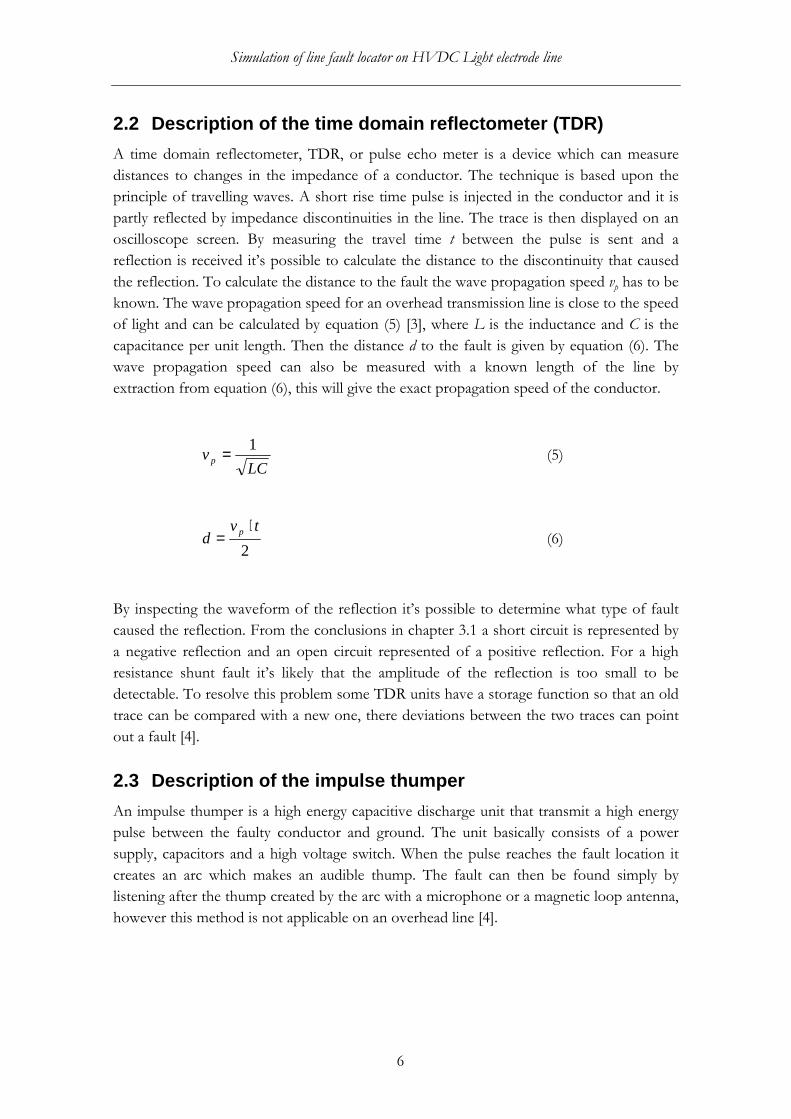
The electrode line model consists of an ideal current source and two frequency dependent

transmission line segments connected through ideal conductors. Table 3.2 shows the

settings of the transmission line model used in PSCAD/EMTDC. An electrode resistance

of 0.2 Ω has been used, which is the highest allowable resistance for the ground electrodes.

Two transmission line segments are used so that a fault can be staged anywhere along the

line by adjusting the individual length of the two segments. Figure 3.2 shows the electrode

line model with one of the two conductors disconnected at both the converter station and

the electrode station, a ground fault has also been placed between the two line segments.


9

Table 3.2 Transmission line model settings in PSCAD/EMTDC.

Frequency dependent (phase) model options

Travel time interpolation On

Curve fitting starting frequency 0.01 [Hz]

Curve fitting end frequency 20000 [Hz]

Total number of frequency increments 1000

Maximum order of fitting for Ysurge 20

Maximum order of fitting for prop. func. 20

Maximum fitting error for Ysurge 0.2 [%]

Maximum fitting error for prop. Func. 0.2 [%]

TLinezambeziTI10

.00

1 [o

hm

]

TLinezambe2T

Tlinezambezi

1

Tlinezambezi

1

Tlinezambe2

1

Tlinezambe2

10.2 [ohm]

0.001 [ohm]

0.001 [ohm]

Fa

ult

Figure 3.2 The electrode line model in PSCAD consists of a grounded current source, two transmission line segments with a ground fault applied between them and a resistor connected to ground representing the electrode .


10

3.2 Modelling of line fault locator

3.2.1 Time domain reflectometer

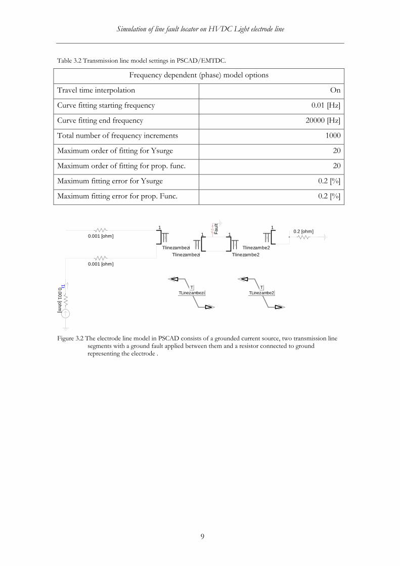
The TDR models are based on the Hipotronics TDR 1150 and the Megger MTDR. Data

for the two models are presented in table 3.3.

Table 3.3 Data for the TDR units [5] [6].

Model TDR 1150 MTDR

Pulse amplitude [V] 25 10

Max. pulse width [µs] 20 10

Max. range [km] 60 50

Sampling rate [MHz] 100 50

Voltage input protection level [V] 480 250

The TDR model consists of a voltage source, a circuit breaker and a voltmeter, see figure

3.3. The circuit breaker is connected to a timing device so that the pulse width can be

controlled.

Initial simulations showed a DC voltage on the electrode line of approximately 10 V. A

10k Ω resistor is therefore connected parallel to the voltmeter to resolve this problem.

The reading of the voltmeter is displayed on a graph that represents the oscilloscope of the

TDR. The time interval of the graphs is chosen so that the whole length of the line is

shown on the graphs.

Two cursors are then placed at the graph, one at the beginning of the generated pulse and

one at the beginning of the reflection. The time interval between the two cursors ∆t is then

used to calculate the distance using equation (6).

TimedBreaker

LogicOpen@t0

BRK150

[oh

m]

Ea

BRK1

10

[ko

hm

]

Figure 3.3 The TDR model, there Ea is the measured voltage.


11

3.2.2 Arc reflection

The Arc reflection model is based on the Hipotronics 5250-30 and the Megger PFL 40

series. Data for the two models are presented in table 3.4.

Table 3.4 Data for the Arc reflection units [5] [6].

Model Voltage [kV] Stored energy [J]

5250-30 0-30 2000

PFL 40 8/16/34 1500

The arc reflection model consists of a voltage source, a capacitor, two circuit breakers and

a voltmeter. The voltage source handles the charging of the capacitor. The capacitor stores

the energy released by the line fault locator. Equation 7 describes the relationship between

the energy stored in a capacitor and the voltage and capacitance.

Circuit breaker one separates the capacitor from the voltage source and circuit breaker two

releases the pulse. The voltmeter represents the oscilloscope of the TDR unit, see

figure 3.4.

2

2VCW

⋅= (7)

C

1 [o

hm

]

Ea

BRK1 BRK2

Figure 3.4 Arc reflection model.


12

3.3 Fault model

The fault model for ground faults consists of a fault module that can be switched on and

off. The fault module is connected in series with a resistor to ground. Two values of the

resistance are used: 1 Ω representing a short circuit to ground and a higher value of 231 Ω

which is the highest likely resistance to trip the differential protection system of the

electrode line, see table 3.5.

The electrode line has a longitudinal differential protection system that is used to detect

ground faults on the line. The protection system measures the current in both ends of the

line with DC current transducers. The system is set to alarm when a difference of 17 A is

detected [7]. This means that ground faults generating a current of 17A and above should

be localised.

The resistance of a fault that can be detected varies along the line due to the voltage drop

in the line. Close to the electrode the voltage to ground is lower than the voltage at the

converter station and a ground fault has to be of lower resistance to be detected by the

differential protection system.

Table 3.5 shows the voltage to ground (acquired by simulations in PSCAD/EMTDC) and

the maximum resistance of a ground fault that leads to an alarm (calculated by ohm’s law)

at increasing distances from the converter station. The calculations is based on a worst case

scenario with one of the electrode line conductors disconnected and the other operating at

it’s maximum current rating of 920 A.

Table 3.5 Voltage to ground and the corresponding fault resistance that leads to an alarm in the differential protection system at increasing distances from the converter station.

Distance [km] Voltage [kV] Resistance [Ω]

0 3,94 231

10 2,86 169

20 2,43 143

30 1,68 99

40 0,85 50


13

4 Simulations Table 4.1 shows a list of the simulations. The simulations are done by changing one

parameter at a time to be able to study changes.

Table 4.1 Issues to investigate.

No Item Issue Simulations

1 Fault type High resistance faults may be

hard to detect. Is the amplitude of

the reflection big enough to

detect?

Ground fault of 1 Ω

Ground fault of 231 Ω

Open circuit.

2 Distance to fault How does the distance from the

measuring point to the fault affect

the result?

5 km

25 km

45 km

3 Pulse width How do different pulse widths

affect the result?

1, 10 and 20 µs

4 Pulse amplitude How do different pulse

amplitudes affect the result?

25 V

10 V

5 Connection How does the connection of the

TDR to the line affect the result?

Conductor-Ground mode.

Conductor-Conductor mode.

6 Parallel line How does a parallel line in

operation affect the result?

On

Off

7 Electrode station

configuration

How does the connection of the

line to the electrode affect the

result?

Connected

Disconnected

8 Arc reflection Does a high voltage pulse

increase the performance of the

TDR?

30kV 2000J Pulse

4.1 Fault type

As default settings, pulse amplitude of 25 V and a pulse width of 10 µs have been used.

The TDR is connected between one conductor and ground as a default with the measured

conductor disconnected at the electrode station.


14

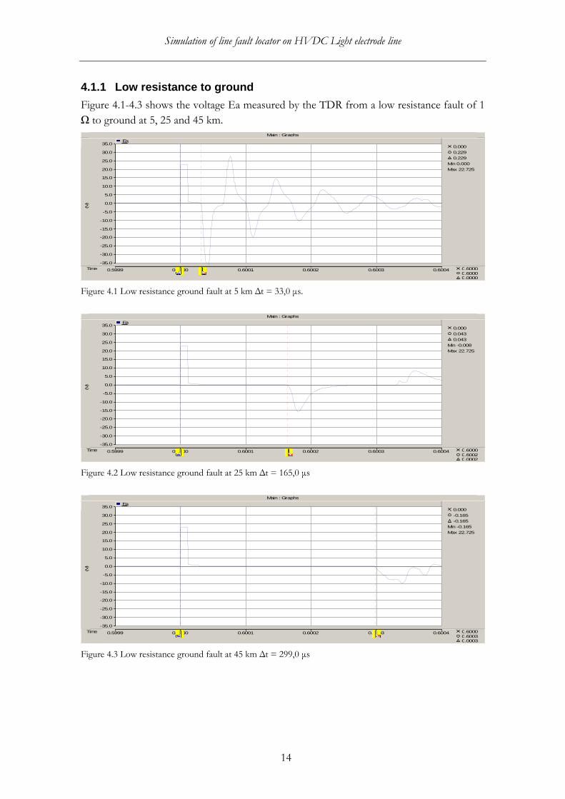
4.1.1 Low resistance to ground

Figure 4.1-4.3 shows the voltage Ea measured by the TDR from a low resistance fault of 1

Ω to ground at 5, 25 and 45 km. Main : Graphs

Time 0.5999 0.6000 0.6001 0.6002 0.6003 0.6004 0.6000 0.6000 0.0000

-35.0

-30.0

-25.0

-20.0

-15.0

-10.0

-5.0

0.0

5.0

10.0

15.0

20.0

25.0

30.0

35.0

(V)

0.000 0.229 0.229

Min 0.000 Max 22.725

Ea

Figure 4.1 Low resistance ground fault at 5 km ∆t = 33,0 µs.

Main : Graphs

Time 0.5999 0.6000 0.6001 0.6002 0.6003 0.6004 0.6000 0.6002 0.0002

-35.0

-30.0

-25.0

-20.0

-15.0

-10.0

-5.0

0.0

5.0

10.0

15.0

20.0

25.0

30.0

35.0

(V)

0.000 0.043 0.043

Min -0.008 Max 22.725

Ea

Figure 4.2 Low resistance ground fault at 25 km ∆t = 165,0 µs

Main : Graphs

Time 0.5999 0.6000 0.6001 0.6002 0.6003 0.6004 0.6000 0.6003 0.0003

-35.0

-30.0

-25.0

-20.0

-15.0

-10.0

-5.0

0.0

5.0

10.0

15.0

20.0

25.0

30.0

35.0

(V)

0.000 -0.165 -0.165

Min -0.165 Max 22.725

Ea

Figure 4.3 Low resistance ground fault at 45 km ∆t = 299,0 µs


15

4.1.2 High resistance to ground

Figure 4.4-4.6 shows the voltage Ea measured by the TDR from a high resistance fault of

231 Ω to ground at 5, 25 and 45 km. Main : Graphs

Time 0.5999 0.6000 0.6001 0.6002 0.6003 0.6004 0.6000 0.6000 0.0000

-35.0

-30.0

-25.0

-20.0

-15.0

-10.0

-5.0

0.0

5.0

10.0

15.0

20.0

25.0

30.0

35.0

(V)

0.006 -0.756 -0.762

Min -4.049 Max 22.726

Ea

Figure 4.4 High resistance ground fault at 5 km ∆t = 33,0 µs

Main : Graphs

Time 0.5999 0.6000 0.6001 0.6002 0.6003 0.6004 0.6000 0.6002 0.0002

-35.0

-30.0

-25.0

-20.0

-15.0

-10.0

-5.0

0.0

5.0

10.0

15.0

20.0

25.0

30.0

35.0

(V)

0.006 -0.147 -0.153

Min -0.147 Max 22.726

Ea


Main : Graphs

Time 0.5999 0.6000 0.6001 0.6002 0.6003 0.6004 0.6000 0.6003 0.0003

-35.0

-30.0

-25.0

-20.0

-15.0

-10.0

-5.0

0.0

5.0

10.0

15.0

20.0

25.0

30.0

35.0

(V)

0.006 -0.360 -0.366

Min -0.742 Max 22.726

Ea



16

4.1.3 Open circuit

Figure 4.7-4.9 shows the voltage Ea measured by the TDR from an open circuit at 5, 25

and 45 km. Main : Graphs

Time 0.5999 0.6000 0.6001 0.6002 0.6003 0.6004 0.6000 0.6000 0.0000

-5.0

0.0

5.0

10.0

15.0

20.0

25.0

30.0

35.0

40.0

(V)

0.247 2.584 2.336

Min 0.247 Max 22.748

Ea

Figure 4.7 Open circuit at 5km ∆t = 33,5µs

Main : Graphs

Time 0.5999 0.6000 0.6001 0.6002 0.6003 0.6004 0.6000 0.6002 0.0002

-5.0

0.0

5.0

10.0

15.0

20.0

25.0

30.0

35.0

40.0

(V)

0.247 0.289 0.042

Min 0.247 Max 22.748

Ea

Figure 4.8 Open circuit at 25km ∆t = 165,0 µs

Main : Graphs

Time 0.5999 0.6000 0.6001 0.6002 0.6003 0.6004 0.6000 0.6003 0.0003

-5.0

0.0

5.0

10.0

15.0

20.0

25.0

30.0

35.0

40.0

(V)

0.246 0.736 0.490

Min 0.246 Max 22.748

Ea

Figure 4.9 Open circuit at 45km ∆t=299,0 µs


17

4.2 Pulse width

The pulse width is a way of controlling the amount of energy applied to a fault.

A simulation of pulse width settings of 1 and 20 µs applied to a high resistance fault 25 km

from the converter station is showed in figure 4.10 and 4.11. The displayed values are the

voltage Ea measured by the TDR.

Main : Graphs

Time 0.5999 0.6000 0.6001 0.6002 0.6003 0.6004 0.6000 0.6002 0.0002

-35.0

-30.0

-25.0

-20.0

-15.0

-10.0

-5.0

0.0

5.0

10.0

15.0

20.0

25.0

30.0

35.0

(V

)

0.006 -0.017 -0.023

Min -0.159 Max 22.653

Ea

Figure 4.10 The reflection from a 1 µs pulse is too small to detect.

Main : Graphs

Time 0.5999 0.6000 0.6001 0.6002 0.6003 0.6004 0.6000 0.6002 0.0002

-35.0

-30.0

-25.0

-20.0

-15.0

-10.0

-5.0

0.0

5.0

10.0

15.0

20.0

25.0

30.0

35.0

(V

)

0.006 0.058 0.052

Min -0.111 Max 22.757

Ea

Figure 4.11 The reflection from a 20 µs pulse where ∆t=165,5 µs.


18

4.3 Pulse amplitude

The affects of higher or lower pulse amplitude is tested by applying a lower voltage of 10 V

in addition to the previous 25 V simulations. The simulations are done with a high

resistance fault, which is likely to be the hardest to detect, at 5, 25 and 45 km and a pulse

width of 10 µs. Figure 4.12-4.14 shows the result, where the displayed values are the


Main : Graphs

Time 0.5999 0.6000 0.6001 0.6002 0.6003 0.6004 0.6000 0.6000 0.0000

-15.0

-10.0

-5.0

0.0

5.0

10.0

15.0

(V)

0.002 -0.303 -0.305

Min -1.620 Max 9.090

Ea

Figure 4.12 High resistance ground fault at 5 km ∆t=33,0 µs

Main : Graphs

Time 0.5999 0.6000 0.6001 0.6002 0.6003 0.6004 0.6000 0.6002 0.0002

-15.0

-10.0

-5.0

0.0

5.0

10.0

15.0

(V)

0.002 0.009 0.006

Min -0.059 Max 9.090

Ea


Main : Graphs

Time 0.5999 0.6000 0.6001 0.6002 0.6003 0.6004 0.6000 0.6003 0.0003

-15.0

-10.0

-5.0

0.0

5.0

10.0

15.0

(V)

0.002 -0.028 -0.030

Min -0.144 Max 9.090

Ea



19

4.4 Connection

By connecting the LFL to both conductors instead of one conductor and ground, another

configuration is achieved. Simulations are done for a high resistance fault and an open line.

Figure 4.15-4.17 shows the high resistance simulations at 5, 25 and 45 km distance from

the converter station. The displayed values are the voltage Ea measured by the TDR.

Main : Graphs

Time 0.6000 0.6002 0.6004 0.6000 0.6000 0.0000

-35.0 -30.0 -25.0 -20.0 -15.0 -10.0 -5.0 0.0 5.0

10.0 15.0 20.0 25.0 30.0 35.0

(V)

0.246 -0.436 -0.682

Min -2.572 Max 22.917

Ea


Main : Graphs

Time 0.6000 0.6002 0.6004 0.6000 0.6002 0.0002

-35.0 -30.0 -25.0 -20.0 -15.0 -10.0 -5.0 0.0 5.0

10.0 15.0 20.0 25.0 30.0 35.0

(V)

0.246 0.263 0.017

Min 0.169 Max 22.917

Ea


Main : Graphs

Time 0.6000 0.6002 0.6004 0.6000 0.6003 0.0003

-35.0 -30.0 -25.0 -20.0 -15.0 -10.0 -5.0 0.0 5.0

10.0 15.0 20.0 25.0 30.0 35.0

(V)

0.246 0.259 0.013

Min -0.093 Max 22.917

Ea



20

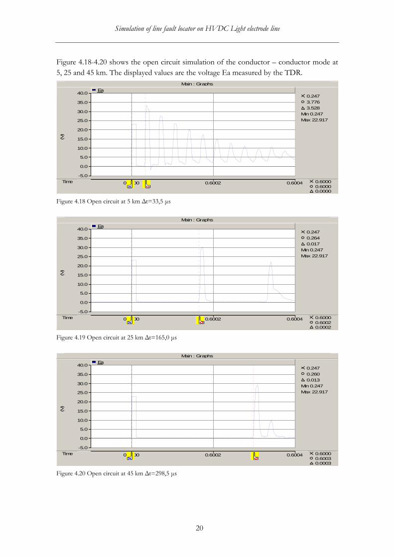
Figure 4.18-4.20 shows the open circuit simulation of the conductor – conductor mode at

5, 25 and 45 km. The displayed values are the voltage Ea measured by the TDR.

Main : Graphs

Time 0.6000 0.6002 0.6004 0.6000 0.6000 0.0000

-5.0

0.0

5.0

10.0

15.0

20.0

25.0

30.0

35.0

40.0

(V)

0.247 3.776 3.528

Min 0.247 Max 22.917

Ea

Figure 4.18 Open circuit at 5 km ∆t=33,5 µs

Main : Graphs

Time 0.6000 0.6002 0.6004 0.6000 0.6002 0.0002

-5.0

0.0

5.0

10.0

15.0

20.0

25.0

30.0

35.0

40.0

(V)

0.247 0.264 0.017

Min 0.247 Max 22.917

Ea


Main : Graphs

Time 0.6000 0.6002 0.6004 0.6000 0.6003 0.0003

-5.0

0.0

5.0

10.0

15.0

20.0

25.0

30.0

35.0

40.0

(V)

0.247 0.260 0.013

Min 0.247 Max 22.917

Ea



21

4.5 Parallel/single line

Parallel lines give a risk of induced voltages that might affect the ability to make accurate

measurements. Therefore a simulation is made with a change in the current in one

conductor.

Figure 4.21 shows the induced voltage at the converter station when di/dt changes from 2

A /ms to 0 A /ms in the parallel conductor. The displayed value is the voltage Ea

measured by the TDR.

Main : Graphs

Time 0.580 0.590 0.600 0.610 0.620 0.630 ... ... ...

0

50

100

150

200

250

300

(V

)

Ea

Figure 4.21 The induced voltage at the converter station from a parallel line.

A simulation with a single line as a reference and for future projects was also made with a

high resistance ground fault at 5, 25 and 45 km. The results are shown in figure 4.22-4.24,

where the displayed values are the voltage Ea measured by the TDR.

Main : Graphs

Time 0.5999 0.6000 0.6001 0.6002 0.6003 0.6004 0.6000 0.6000 0.0000

-35.0 -30.0 -25.0 -20.0 -15.0 -10.0 -5.0 0.0 5.0

10.0 15.0 20.0 25.0 30.0 35.0

(V)

0.006 -0.763 -0.769

Min -3.734 Max 22.730

Ea



22

Main : Graphs

Time 0.5999 0.6000 0.6001 0.6002 0.6003 0.6004 0.6000 0.6002 0.0002

-35.0 -30.0 -25.0 -20.0 -15.0 -10.0 -5.0 0.0 5.0

10.0 15.0 20.0 25.0 30.0 35.0

(V)

0.006 -0.028 -0.034

Min -0.337 Max 22.730

Ea


Main : Graphs

Time 0.6000 0.6002 0.6004 0.6000 0.6003 0.0003

-35.0 -30.0 -25.0 -20.0 -15.0 -10.0 -5.0 0.0 5.0

10.0 15.0 20.0 25.0 30.0 35.0

(V)

0.006 -0.030 -0.036

Min -0.030 Max 22.730

Ea


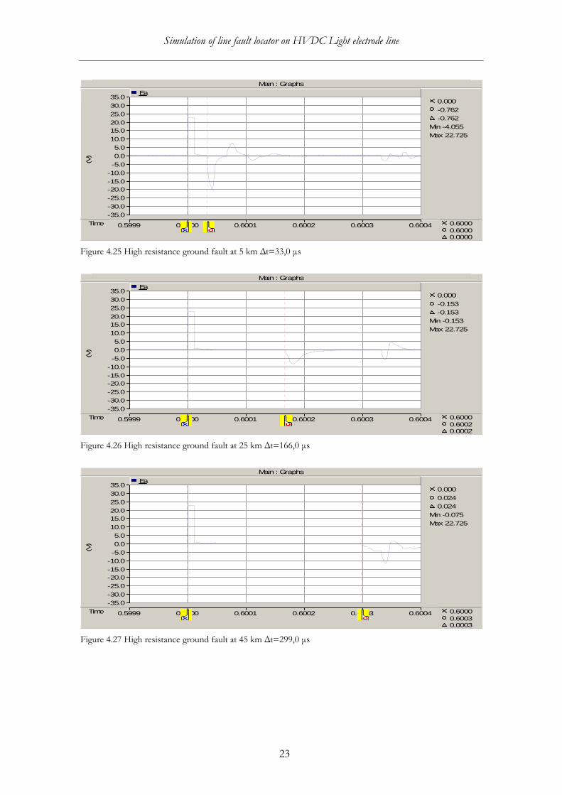
4.6 Electrode station configuration

In case of problems with the remote controlled disconnectors at the electrode station a

simulation is made with the disconnectors closed. The simulations are made with a high

resistance fault at 5, 25 and 45 km, see figure 4.25-4.27. The displayed values are the



23

Main : Graphs

Time 0.5999 0.6000 0.6001 0.6002 0.6003 0.6004 0.6000 0.6000 0.0000

-35.0 -30.0 -25.0 -20.0 -15.0 -10.0 -5.0 0.0 5.0

10.0 15.0 20.0 25.0 30.0 35.0

(V)

0.000 -0.762 -0.762

Min -4.055 Max 22.725

Ea


Main : Graphs

Time 0.5999 0.6000 0.6001 0.6002 0.6003 0.6004 0.6000 0.6002 0.0002

-35.0 -30.0 -25.0 -20.0 -15.0 -10.0 -5.0 0.0 5.0

10.0 15.0 20.0 25.0 30.0 35.0

(V)

0.000 -0.153 -0.153

Min -0.153 Max 22.725

Ea


Main : Graphs

Time 0.5999 0.6000 0.6001 0.6002 0.6003 0.6004 0.6000 0.6003 0.0003

-35.0 -30.0 -25.0 -20.0 -15.0 -10.0 -5.0 0.0 5.0

10.0 15.0 20.0 25.0 30.0 35.0

(V)

0.000 0.024 0.024

Min -0.075 Max 22.725

Ea



24

4.7 Arc reflection

Simulations with a high voltage pulse representing the Arc reflection method are done to

a high resistance ground fault at 5, 25 and 45 km, see figure 4.28-4.30. The displayed values

are the voltage Ea measured by the TDR.

Main : Graphs

0.2999 0.3000 0.3001 0.3002 0.3003 0.3004 0.3000 0.3000 0.0000

-40.0k-35.0k-30.0k-25.0k-20.0k-15.0k-10.0k-5.0k0.0 5.0k

10.0k15.0k20.0k25.0k30.0k35.0k40.0k

y (V

)

0.0069k -3.6001k -3.6070k

Min -5.5995k Max 29.6459k

Ea


Main : Graphs

0.2999 0.3000 0.3001 0.3002 0.3003 0.3004 0.3000 0.3002 0.0002

-40.0k-35.0k-30.0k-25.0k-20.0k-15.0k-10.0k-5.0k0.0 5.0k

10.0k15.0k20.0k25.0k30.0k35.0k40.0k

y (V

)

0.0069k -0.2725k -0.2794k

Min -0.2084k Max 29.6459k

Ea



25

Main : Graphs

0.2999 0.3000 0.3001 0.3002 0.3003 0.3004 0.3000 0.3003 0.0003

-40.0k-35.0k-30.0k-25.0k-20.0k-15.0k-10.0k-5.0k0.0 5.0k

10.0k15.0k20.0k25.0k30.0k35.0k40.0k

y (V

)

0.0069k 0.0372k 0.0302k

Min 0.0069k Max 29.6459k

Ea



26

5 Results and analysis To be able detect a line fault with a LFL the reflection from an injected pulse has to be well

defined with significant amplitude and a preferable low rise time. High amplitude of the

reflection makes it easier to distinguish from smaller reflections caused by discontinuities in

the line. A low rise time makes it easier to point out a more precise arrival time for the

reflection and there by give a more accurate distance to the fault.

The results from the simulations are presented in tables with the travel time for the pulse

and the amplitude of the reflection. Further is the distance to the fault calculated by

equation (6) and an error is calculated by subtracting the actual distance from the calculated

distance.

The propagation speed that has been used to calculate the distances is 302,35 m/µs which

been obtained as a mean value through simulations at 45 km distance. The odd result of a

higher propagation speed than the speed of light probably comes from an inefficiently long

solution time step setting of 0,5 µs. Simulations show that by shortening the solution time

step a more accurate propagation speed can be obtained. However as a shorter solution

time step increases the simulation time the longer time step has been chosen.

5.1 Fault type

5.1.1 Low resistance ground fault

The results of the low resistance simulations (figure 4.1-4.3) are shown in table 5.1. From

the results can we see that the reflections are of reversed polarity as indicated in section 2.1.

The amplitudes of the reflections are high at a close distance but attenuate as the distance

to the faults increases. The rise time of the fault reflections is low at a close distance but

increases with increased distance. The error seams to increase with increasing distance and

the maximum error is 201 m which is approximately 0,4% of the total length of the line.

Over all the low resistance fault of 1 Ω is highly detectable in the simulation.

Table 5.1 Results from the low resistance simulation.

Fault

distance

[km]

Pulse

amplitude

[V]

Pulse

width

[µs]

Reflection

amplitude

[V]

Travel

time [µs]

Calculated

distance

[m]

Error

[m]

5 25 10 -35 33,0 4 989 -11

25 25 10 -15 165,0 24 944 -56

45 25 10 -10 299,0 45 201 201


27

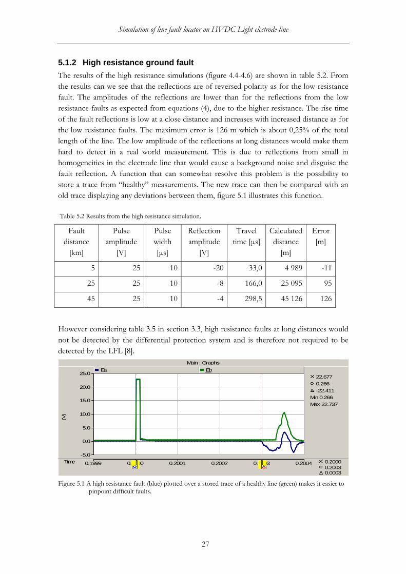
5.1.2 High resistance ground fault

The results of the high resistance simulations (figure 4.4-4.6) are shown in table 5.2. From

the results can we see that the reflections are of reversed polarity as for the low resistance

fault. The amplitudes of the reflections are lower than for the reflections from the low

resistance faults as expected from equations (4), due to the higher resistance. The rise time

of the fault reflections is low at a close distance and increases with increased distance as for

the low resistance faults. The maximum error is 126 m which is about 0,25% of the total

length of the line. The low amplitude of the reflections at long distances would make them

hard to detect in a real world measurement. This is due to reflections from small in

homogeneities in the electrode line that would cause a background noise and disguise the

fault reflection. A function that can somewhat resolve this problem is the possibility to

store a trace from “healthy” measurements. The new trace can then be compared with an

old trace displaying any deviations between them, figure 5.1 illustrates this function.

Table 5.2 Results from the high resistance simulation.

Fault

distance

[km]

Pulse

amplitude

[V]

Pulse

width

[µs]

Reflection

amplitude

[V]

Travel

time [µs]

Calculated

distance

[m]

Error

[m]

5 25 10 -20 33,0 4 989 -11

25 25 10 -8 166,0 25 095 95

45 25 10 -4 298,5 45 126 126

However considering table 3.5 in section 3.3, high resistance faults at long distances would

not be detected by the differential protection system and is therefore not required to be

detected by the LFL [8].

Main : Graphs

Time 0.1999 0.2000 0.2001 0.2002 0.2003 0.2004 0.2000 0.2003 0.0003

-5.0

0.0

5.0

10.0

15.0

20.0

25.0

(V)

22.677 0.266 -22.411

Min 0.266 Max 22.737

Ea Eb

Figure 5.1 A high resistance fault (blue) plotted over a stored trace of a healthy line (green) makes it easier to pinpoint difficult faults.


28


Fault

distance

[km]

Pulse

amplitude

[V]

Pulse

width

[µs]

Reflection

amplitude

[V]

Travel

time [µs]

Calculated

distance

[m]

Error

[m]

5 25 10 -20 33,0 4 989 -11

25 25 10 -8 166,0 25 095 95

45 25 10 -4 298,5 45 126 126

5.1.3 Open circuit

The results of the open circuit simulations (figure 4.7-4.9) are shown in table 5.3. From the

results can we see that the reflections are of the same polarity as the original pulse,

indicating that the fault is of a high resistance series character. The amplitudes of the

reflections are higher at a close distance but attenuate as the distance to the faults increases

as for the ground faults. The rise time of the fault reflections seams to be lower than for

the ground faults although the error shows no sign of improvement with a maximum error

of 201 m. The simulations show that an open circuit fault ought to be easier to detect than

ground faults due to the high amplitudes of the reflections.

Table 5.3 Results from open circuit simulation.

Fault

distance

[km]

Pulse

amplitude

[V]

Pulse

width

[µs]

Reflection

amplitude

[V]

Travel

time [µs]

Calculated

distance

[m]

Error

[m]

5 25 10 32 33,5 5 064 64

25 25 10 17 165,0 24 944 -56

45 25 10 10 299,0 45 201 201

5.2 Pulse width

The results of the pulse width simulations (figure 4.10-4.11) that were applied to a high

resistance ground fault are shown in table 5.4. The amplitudes of the reflections are higher

with a longer pulse width, this is probably from the increased amount of energy delivered

to the fault. The shorter pulse width of 1 µs is hardly detectable and a pulse width of at

least 10 µs preferable 20 µs seams suitable for a longer overhead line. A possible

application for a short pulse width is if the fault is close to the measuring point and longer

pulse widths would disguise it. The rise time of the fault reflections seams to be unaffected

by the longer pulse width. Further shows the error no difference between the two

detectable traces.


29

Table 5.4 Results from the pulse width simulation.

Fault

distance

[km]

Pulse

amplitude

[V]

Pulse

width

[µs]

Reflection

amplitude

[V]

Travel

time [µs]

Calculated

distance

[m]

Error

[m]

25 25 1 0 - - -

25 25 10 -8 166,0 25 095 95

25 25 20 -13 165,5 25 019 19

5.3 Pulse amplitude

The results of the pulse amplitude simulations (figure 4.12-4.14) that were applied to a high

resistance ground fault are shown in table 5.5. The amplitudes of the 10 V pulse reflections

are roughly in the same area as for the 25 V pulse amplitudes calculated as fractions of the

original pulses. The rise time of the fault reflections seams also to be unaffected by

differences in the pulse amplitude, this is somewhat expected due to the linearity of the

fault model. Further shows the error no bigger difference between the different pulse

amplitudes. The simulations show no difference between the pulse amplitudes and no

conclusions can be made stating that higher or lower pulse amplitude is better. A possible

reason for choosing lower pulse amplitude would be measurements on low voltage control

cables reducing the risk of interference. However as the LFL is to be used on an overhead

line this is not an issue of interest and higher pulse amplitude should be preferred due to

the higher energy delivered to the fault.

Table 5.5 Results from the pulse amplitude simulation.

Fault

distance

[km]

Pulse

amplitude

[V]

Pulse

width

[µs]

Reflection

amplitude

[V]

Travel

time [µs]

Calculated

distance

[m]

Error

[m]

5 10 10 -8 33,0 4 989 -11

25 10 10 -3 167,0 25 246 246

45 10 10 -2 298,5 45 126 126

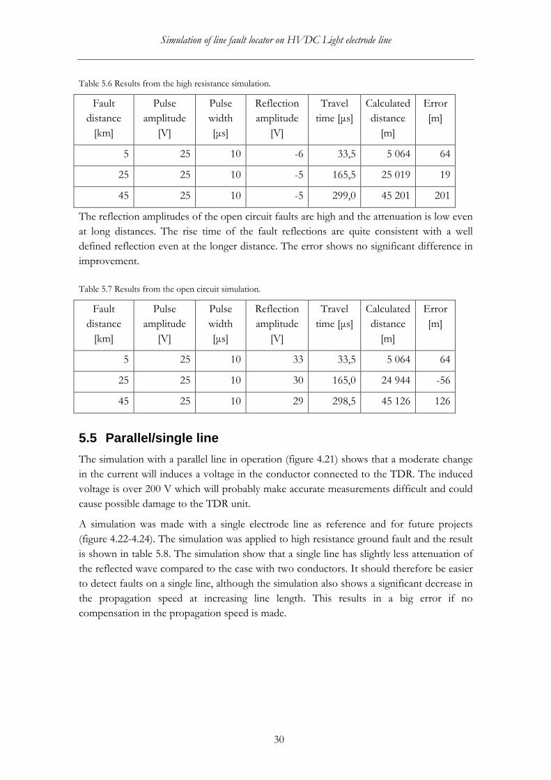
5.4 Connection

The results of the simulations with the TDR connected between the two conductors (figure

4.15-4.20) are shown in table 5.6 for the high resistance fault and in table 5.7 for the open

circuit. The reflections of the high resistance faults are lower at short distances although

they are more constant throughout the length of the line. The rise time of the fault

reflections are also quite consistent with a well defined reflection even at the longer

distance. The error shows no significant improvement to previous simulations.


30


Fault

distance

[km]

Pulse

amplitude

[V]

Pulse

width

[µs]

Reflection

amplitude

[V]

Travel

time [µs]

Calculated

distance

[m]

Error

[m]

5 25 10 -6 33,5 5 064 64

25 25 10 -5 165,5 25 019 19

45 25 10 -5 299,0 45 201 201

The reflection amplitudes of the open circuit faults are high and the attenuation is low even

at long distances. The rise time of the fault reflections are quite consistent with a well

defined reflection even at the longer distance. The error shows no significant difference in

improvement.

Table 5.7 Results from the open circuit simulation.

Fault

distance

[km]

Pulse

amplitude

[V]

Pulse

width

[µs]

Reflection

amplitude

[V]

Travel

time [µs]

Calculated

distance

[m]

Error

[m]

5 25 10 33 33,5 5 064 64

25 25 10 30 165,0 24 944 -56

45 25 10 29 298,5 45 126 126

5.5 Parallel/single line

The simulation with a parallel line in operation (figure 4.21) shows that a moderate change

in the current will induces a voltage in the conductor connected to the TDR. The induced

voltage is over 200 V which will probably make accurate measurements difficult and could

cause possible damage to the TDR unit.

A simulation was made with a single electrode line as reference and for future projects

(figure 4.22-4.24). The simulation was applied to high resistance ground fault and the result

is shown in table 5.8. The simulation show that a single line has slightly less attenuation of

the reflected wave compared to the case with two conductors. It should therefore be easier

to detect faults on a single line, although the simulation also shows a significant decrease in

the propagation speed at increasing line length. This results in a big error if no

compensation in the propagation speed is made.


31

Table 5.8 Results from the single line simulation.

Fault

distance

[km]

Pulse

amplitude

[V]

Pulse

width

[µs]

Reflection

amplitude

[V]

Travel

time [µs]

Calculated

distance

[m]

Error

[m]

5 25 10 -20 32,0 4 838 -162

25 25 10 -10 169,0 25 549 549

45 25 10 -6 306,50 46 335 1 335

5.6 Electrode station configuration

The results of the simulations with the disconnectors closed at the electrode station (figure

4.25-4.27) are shown in table 5.9. The reflection amplitudes show the same result as for the

high resistance faults with the disconnectors open. Further shows the simulations the same

attenuation and rise time as the high resistance simulation. At long distances the fault

reflection can be disguised by the reflection from the electrode and measurements should

therefore preferable be made with the disconnectors open.

Table 5.9 Results from the electrode station simulation.

Actual

fault

distance

[km]

Pulse

amplitude

[V]

Pulse

width

[µs]

Reflection

amplitude

[V]

Travel

time [µs]

Calculated

distance

[m]

Error

[m]

5 25 10 -20 33,0 4 989 -11

25 25 10 -8 166,0 25 095 95

45 25 10 -4 299,0 45 201 201

5.7 Arc reflection

The results from the Arc reflection simulations (figure 4.28-4.30) applied to a high

resistance fault are shown in table 5.10. The simulations show no difference from the low

voltage pulse simulations on high resistance faults. This is probably because of the linear

fault model and a better nonlinear model should be developed if this method is to be

simulated further.


32

Table 5.10 Results from the Arc reflection simulation.

Fault

distance

[km]

Pulse

amplitude

[kV]

Pulse

width

[µs]

Reflection

amplitude

[kV]

Travel

time [µs]

Calculated

distance

[m]

Error

[m]

5 30 10 -27 33,5 5 064 64

25 30 10 -10 166,0 25 095 95

45 30 10 -5 297,5 44 975 -25


33

6 Conclusions and future work The results of the simulations show that it is possible to detect faults of both open circuit

and ground fault types with a suitable TDR unit. Ground faults with high resistance

occurring at long distances can be hard to detect due to the low reflection amplitudes. This

problem can somewhat be resolved with a function that lets the user compare an old trace

of a “healthy” line with the new trace. The study shows that most of the faults can be

detected and the distance to the fault can be calculated within an accuracy of ± 250 m,

although further studies with field measurements and staged line faults should determine a

more precise accuracy of the final LFL.

The pulse width of the TDR needs to be at least 10 µs, preferable 20 µs to deliver high

enough energy to the fault to create a detectable reflection. The pulse amplitude seams to

be of less significance in this simulation, although higher pulse amplitude is likely to be

more suitable in a real measurement due to the higher energy delivered to the fault. The

Hipotronics TDR 1150 is a unit that fulfil these requirements and should therefore be able

to work as a LFL on the electrode line.

Further shows the simulation with the TDR connected between the two conductors that

this is a possible way of decreasing the rise time of the reflections and thereby increasing

the accuracy, however further field studies can clarify this.

The simulations show a risk of high voltage transients if measurements are done with a

parallel line in operation. This is due to induction from current changes in the parallel

conductor and could cause possible damage to a TDR unit.

In the case with a single conductor the simulation shows less attenuation of the reflections

and a fault should therefore be easier to detect. Although a significant decrease of the wave

propagation speed at increasing distance to the fault was detected. This results in a

substantial error in the calculated distance if no compensations are made to the

propagation speed.

Simulations with the electrode line connected to the electrode shows that high resistance

ground faults close to the electrode station can be disguised by the reflection of the

electrode. Measurements should therefore preferable be made with the disconnectors open

at the electrode station.

The simulation of the Arc reflection method, which combines the use of a TDR and a high

energy impulse generator, shows no improvement to the stand-alone TDR unit. This can

be explained with the linear fault model and a better fault model has to be developed to

study this method further.


34

References

1. ABB AB (2010) Easy introduction for laypersons [Electronic] ABB AB Available: <http://www.abb.com/industries/us/9AAF400197.aspx> [2010-04-06]

2. ABB AB (2010) Caprivi Link Interconnector [Electronic] ABB AB Available: <http://www.abb.com/cawp/gad02181/a93201eafb31ba07c125738000468455.aspx> [2010-04-06]

3. Hileman, Andrew R (1999) Insulation Coordination for Power Systems Marcel Dekker

4. Gill, Paul (2008) Electrical Power Equipment Maintenance and Testing CRC Press

5. Hipotronics (2010) Products - Cable Fault Locating Equipment [Electronic] Hipotronics Available: <http://www.hipotronics.com/products/cable-fault-locating-equipment/> [2010-04-06]

6. Megger (2010) PFL40A-1500 [Electronic] Megger Available: <http://www.megger.com/se/products/ProductDetails.php?ID=1227&Description= > [2010-04-06]

7. ABB AB 1JNL100119-686 HVDC Protection System Unpublished manuscript ABB AB

8. ABB AB 06MR0005 Rev.00 Caprivi Link Interconnector Converter Stations Project Volume 3 Sec 7.1.12.2 Unpublished manuscript ABB AB

Simulation of line fault locator on HVDC Light electrode line344138/FULLTEXT01.pdf · BACHELOR’S...

Documents

Transcript of Simulation of line fault locator on HVDC Light electrode line344138/FULLTEXT01.pdf · BACHELOR’S...