Sequential detection of almost-harmonic signals - … · Sequential Detection of Almost-Harmonic...

IEEE TRANSACTIONS ON SIGNAL PROCESSING, VOL. 51, NO. 2, FEBRUARY 2003 395

Sequential Detection of Almost-Harmonic SignalsStefano Marano, Vincenzo Matta, and Peter Willett, Senior Member, IEEE

Abstract—To detect a purely harmonic signal, it is difficult tobeat a fast Fourier transform (FFT). However, when the signal isvery long and weak, Parker and White have shown that a sequen-tial probability ratio test (SPRT) operating on magnitude-squareFFT data is far more efficient. Indeed, both from a numerical-errorperspective and in terms of robustness against a deviation from aprecisely tonal signal, the block-FFT/SPRT idea is very appealing.Here, the approach is extended to the case that the frequency isunknown, and expressions are developed for performance both interms of detection and of sample number. The approach is appli-cable to a large number of practical problems, but particular at-tention is paid to thecontinuous gravitational wave(GW) example.The computational savings as compared with a fixed test vary asa function of signal strength, block length, bandwidth and oper-ating point; however, gains of a factor of two are easy. That thesegains are not more exciting relates mostly to the underlying FFTstructure; although many SPRTs “end early,” it is difficult to takeadvantage of that with an efficient FFT algorithm. However, theprogressive reduction of the number of working SPRTs implies asubstantial reduction of the ensemble of the candidate frequencieswith time, which is an appealing feature, particularly in the GWcase.

Index Terms—Average sample number, detection, gravitationalwaves, numerical efficiency, sequential testing.

I. INTRODUCTION

A NUMBER of problems of practical interest may be formu-lated as the detection, in white Gaussian noise, of almost-

sinusoidal signals, namely, of sinusoids with slowly varyingphase. For instance, this model has been found to be appropriatefor addressing the detection of weak signals that require long in-tegration times, as is the case of some acoustic signals [2], or ofon/off keyed coherent lightwave transmission links, degradedby laser phase noise, as considered in [3]. Another example ofparticular interest to us is the detection of so-called continuous,or periodic, gravitational waves (GWs), which are slowly fre-quency-modulated harmonic signals; see [4]–[6]. In many cases,and in particular in the GW one, the nominal frequency is an un-known parameter.

In the acoustic and optical signal cases mentioned, the phasevariation may be considered a stochastic process and ultimatelya nuisance term. In the GW case, however, the modulationcharacteristics carry important physical information about thesource position in the sky and should be estimated if possible.

Manuscript received January 24, 2002; revised September 12, 2002. The as-sociate editor coordinating the review of this paper and approving it for publi-cation was Prof. Xiaodong Wang.

S. Marano and V. Matta are with DIIIE, Università degli Studi di Salerno,Fisciano, Italy (e-mail: [email protected]; [email protected]).

P. Willett is with the Electrical and Computer Engineering Depart-ment, University of Connecticut, Storrs, CT 06269 USA (e-mail: [email protected]).

Digital Object Identifier 10.1109/TSP.2002.806981

In either case, a conventional detection procedure, based on ageneralized likelihood ratio test (GLRT), would provide suchestimates. Unfortunately, the GLRT requires the computationof an exceedingly large matched filter. To give an idea of thesizes involved, let us say that the signal should be collectedat least for several months, at a sampling frequency of somekilohertz. Thus, the desiredphase trackingmay be impossiblewith the usual computational resources.

In all three cases discussed above, it is the phase variation thatmakes the detection procedure complicated. A possible way tocircumvent this is to divide the observation interval into shortframes in which the phase variation may be neglected. In eachsuch segment, asingle-framedetection statistic is computed(dispensing with the phase tracking problem), and these are ul-timately combined to form the overall statistic. With this ap-proach of segmentation, only a small amount of computation isrequired for each frame, whereas the alternative may be a com-putationally expensive task at the end of the whole observationtime. The segmented procedure is, in addition to quicker, morerobust both in terms of modeling assumptions (deviations fromthe assumed phase model) and in terms of implementation; theseaspects are crucial for the GW application. The price paid is inthe required signal energy to achieve a specified detection per-formance.

The performance loss was found in [2] and [3] in the fixed-length detection context to be surprisingly low. In the presentpaper, we consequently extend the idea to a sequential scenarioin which the number of frames is not fixeda priori: It is the par-ticular statistical realization that determines how many framesare needed to comply with the prescribed performance level.We deal with the design of a sequential detector for almost-si-nusoidal signals with unknown amplitude and frequency, af-fected by phase drift, and embedded in white Gaussian noise.The paper is organized as follows. Section II introduces thenecessary background on the sequential probability ratio test(SPRT); the classical results relating detection performance tothresholds are given, as are the approximations to the averagenumber of samples necessary to come to a decision. A nov-elty here is that an explicit approximation to the probabilitydensity function (pdf) of the sample number is also presented.In Section III, we discuss detection of pure and noncoherentsinewaves, and in Section IV, the overall detection scheme is de-veloped. It comprises preprocessing by magnitude-square FFTs,a bank of SPRTs each matched to an (approximate) center fre-quency, and an eventual fusion of the output from each. Theoverall system-level performance is developed and comparedwith simulation; the previous sample-number pdf was neces-sary for this. In Section V, an accurate evaluation of the com-putational burden is accomplished, and Section VI offers con-cluding remarks.

1053-587X/03$17.00 © 2003 IEEE

396 IEEE TRANSACTIONS ON SIGNAL PROCESSING, VOL. 51, NO. 2, FEBRUARY 2003

II. SPRT

A. Background and Familiar Performance Measures

Let us consider the following hypothesis test:

(1)

where are zero-mean Gaussian random vari-ables ( s), independent and identically distributed (i.i.d.), andwhere represents the (constant) signal to be detected.In the case that is known (and s variance as well), wehave a simple hypothesis test, whereas in the presence of anunknown parameter (e.g., known only to be positive), then(1) is composite. Assume for now thatis known. In order todecide between the occurrence of or , given a set of ob-servations , it is natural to resort to theNeyman–Pearson approach; this leads to the fixed-sample-size(FSS) test based on the log-likelihood ratio , which usesa given number of received samples. Specifically

choosechoose

(2)

The above test maximizes the detection probability for a givenfalse alarm probability, and according to the latter, the appro-priate threshold level is chosen. Here, is the log-likeli-hood ratio per sample:

(3)

where and are the pdfs of the sample underthe hypotheses and , respectively. If the white Gaussianmodel is in force, as assumed above, the log-likelihood ratio be-comes , where is the noise variance.

As an alternative to the FSS test, one that is particularlypleasing when the sample numberis not a priori assigned,we can resort to the well-known SPRT [7]:

choosechoose

take another sample(4)

where we note the presence of two threshold levels, and thepeculiarity of a random number of samples, say, needed forthe test to come a stop.

It is very easy to derive the approximate relationships:

(5)

(a powerful tool to make this computation is to build a martin-gale process based on the log-likelihood ratio and proceedingas in [8, pp. 341–343]), which give the recipe for setting thethreshold levels, and which hold provided that is a valid

log-likelihood ratio, regardless of the simple model (1) being inforce. Here

Pr decide is in force

Pr decide is in force (6)

are the nominal values (subscript) of the detection and falsealarm probabilities, respectively.

Similarly, the following approximations give the averagesample number (ASN) , which the test requires [7]:

under

under (7)

where and , denote the statistical expectation andthe pdf, according to theth hypothesis. Here, is thedivergence between the pdfs measured in nats (see [9]), whereas

(8)

Equation (7) may be derived assuming i.i.d. samples in both thehypotheses and but are otherwise valid for arbitraryand . If the model of (1) is assumed, then in (7), we have

. Usually, the above aver-ages are used to quantify the duration of the test. However, if amore complete statistical characterization be required, it is alsopossible to derive an approximate distribution of, as will bediscussed in Section II-B.

It has been shown by Wald that, for given and , theASN pertaining to the SPRT is less than the ASN of any othersequential test (that eventually terminates with probability one),both under and under [7]. Since the FSS test is a partic-ular case of a sequential procedure in which the random samplenumber has vanishing variance, we conclude that SPRT is op-timum in the sense that it minimizes the average sample numberfor given performances amongst all fixed- and variable-lengthtests.

A central concern is the following: What happens if the pdfactually in force is a certain , different from bothand assumed at the design stage? In other words, (7) holdstrue in nominal conditions, and (5), which relates thresholds toperformance, can be used only in nominal operating situations:What happens when neither nor is true?

To elaborate, let us assume that the i.i.d. samples actuallycollected by the detection device follow a certain pdf , anddenote by this adjoint hypothesis, e.g., with reference tomodel (1) with , let us assume that the value of isdifferent from that assumed at the design stage. Let us introducethe function implicitly defined through the following twoconditions:

(9)

MARANO et al.: SEQUENTIAL DETECTION OF ALMOST-HARMONIC SIGNALS 397

Then it can be shown that [7]

Pr choosing is in force

(10)

Similarly, with regard to the ASN under non-nominal operatingenvironments, it can be shown that [7]

(11)

where refers to expectation under . As for (7), a nice in-formation theoretic formulation of the above involves the diver-gence

(12)

Before concluding the section, we stress that all the givenapproximations are fair when the absolute value of the meanand the standard deviation of the log-likelihood ratio per sample

are much less than and under the actual distribu-tion of the samples . This basically amountsto ignoring the likelihood ratio threshold overshoots,which is a reasonable assumption if we require that the (random)sample number is large. Equivalently, the inherent approxi-mations are fair if the signal-to-noise ratio (SNR) (per sample)is small enough and/or if the nominal performances are suf-ficiently tight, i.e., false alarm probability very small and de-tection probability close to unity. In this paper, we assume thatthe above conditions are substantially met; if this were not thecase, more sophisticated mathematical tools such as nonlinearrenewal theory may be necessary for taking into account thethreshold overshoots, see [10]–[12].

It turns out that we will require a more precise probabilisticexpression for the efficiency of an SPRT. Equation (7) providesus the first moment of , but a full pdf of is given in the nextsubsection.

B. Distribution of the Sample Number for a SPRT

In this section, we postulate an analytical expression for thedistribution of the number of samples needed to reach a decisionand compare it with simulated data. We find that the fit is good,and hence, we will use the expression in the sequel.We have thefollowing in the literature.

• Let be i.i.d. random variables withand VAR . Let , and define

, with . The distributionof is found (see [13, p. 138]).

• Let be a Brownian motion with drift , wherethe variance of the increment is .Assume , and let the first time thatequals . The distribution of is found (see [14, p. 363]).

The former of these relates to discrete time, whereas the latter isformulated in a continuous framework. Both are very similar toour sequential procedure but for a single threshold. It turns out,respectively, that we have the following.

• and

Pr

• and

Pr

The distribution of the normalizedfirst passage timeis the samein the two cases. The relevant density is referred to asWald’s pdf (sometimes called inverse Gaussian), whose expres-sion is [13, p. 138]

(13)

being the step function, where for the two cases, we have,respectively

VARand (14)

It is easily seen that (with a slight abuse of notation), and VAR . Moreover, for ,

the cumulative distribution function is [13, p. 141]

(15)

where is the standard Gaussian exceedance probabilityfunction.

Coming back to our problem of characterizing the randomsample number , we postulate that is approximatelydistributed just as , with parameter VAR .Then, the distribution of the normalized variabledepends on a single parameter. We already have an analyticalexpression for ; thus, should the variance of be found,the distribution would be completely determined. Thiscomputation may be done by means of the same Martingaleapproach yielding (5) and (7). The final results are the fol-lowing approximations [15]: VAR VAR

and VARVAR / ,

where VAR denotes the variance computed underand . Accounting for the previously adopted single-thresholdapproximation (i.e., under , and under

), these formulas simplify to the following:

VAR VAR

VAR VAR (16)

Alternatively, one can assume that follows Wald’sdistribution , with parameter computed directly by (14),where, referring for instance to the first, is replaced with

and with , under ; similarly, under , isreplaced with and with . The two alternatives can beshown to give the same results for large and small .


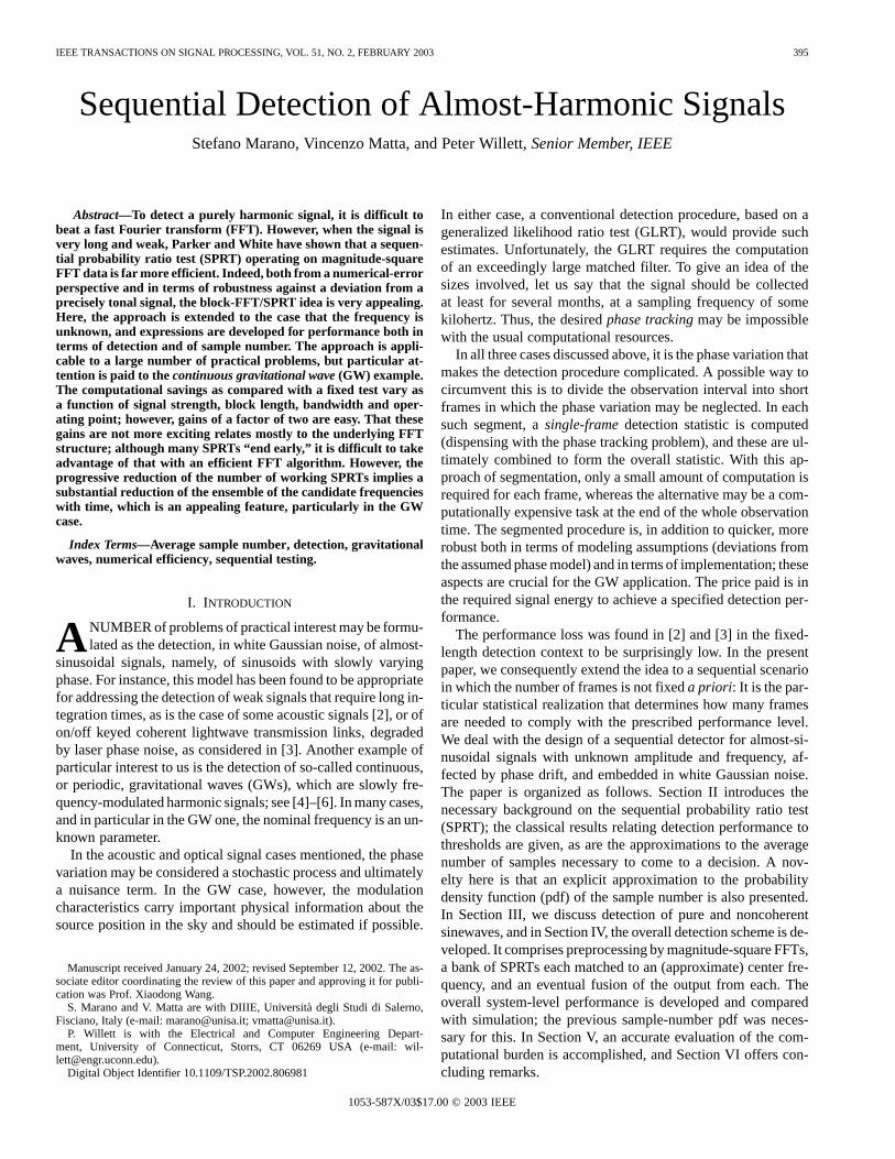
Fig. 1. Comparison between theoretical distribution (solid line) and empiricaldistribution (dashed line) of the normalized sample number. The left plotspertain to Wald’s distributionF (x), whereas the right ones pertain toTartakovsky’s distributionF (x). Simulations, obtained with 50 000 MonteCarlo runs refer toH , with P = 10 . For clarity, the vertical axes use aGaussian scale.

The left plots of Fig. 1 compare distribution (15) withsimulated data.1 It is seen that in the range and

, which is of interest for most applications, thefit is very accurate. Less precise results are obtained with lesssevere test performances, as expected. A possible refinementcan be attained by relaxing the single-threshold assumption;this has been done by Tartakovsky [16], which obtainedexactformulas for the stopping time distribution in the case ofa Brownian motion process. Tartakovsky’s formula, whichcan be easily applied to our discrete model in view of theassumptions detailed at the end of previous subsection, is in theform of a series expansion. The right plots of Fig. 1 compareTartakovsky’s formula with simulated data, confirming a bettermatching for larger error probabilities. Tartakovky’s formulaeare indeed more accurate, but it appears that (15) and (16) [or(14)] are sufficient, and since they are much simpler, we usethem.

III. SEQUENTIAL DETECTION OFHARMONIC SIGNALS

A. Pure Sine Waves

One difficulty arises for the SPRT when the signal to be de-tected is not constant. If we replace the constantunder bya signal sequence in (1), the i.i.d. property is lost. The simplerelationships given above lose validity: The SPRT is easy to im-plement, but its ASN analysis is less clear.

If we consider zero-mean Gaussian i.i.d. noise samples andlet be the signal energy collected up to thesample, then it has been shown that

underunder

(17)

1Simulated data of Fig. 1 refer to the noncoherent detection of almost har-monic signals of known frequency, reducing to a noncentral-� versus cen-tral-� hypothesis testing; more on this later. Wald’s distribution uses expres-sions (14).

where we recall that is the random number of samples ofthe SPRT. The above formula, derived in [17] via a Martin-gale approach, is a particular case of the more general result ac-cording to which the SPRT minimizes theinformational quan-tity among all tests achieving the same performances(see [18] for a lucid and accessible information theoretic per-spective of similar results).

In particular, if we assume that , with, and known parameters, then (17) leads to

underunder

(18)

which, when compared with (7) with , re-veals that the sequential detection of a sinusoidal signal achievesthe same performance as for a constant signal, provided that theconstant value is replaced by theeffectivevalue .

Sequential detection of sinusoids of known frequency hasbeen investigated in [1], where an equivalent of (18) is found.Now, when the signal to be detected is not only nonconstant butalso contains unknown parameters, it is easy to generalize test(2); a commonly adopted solution is represented by the so-calledgeneralized likelihood ratio test (GLRT). Unfortunately, it isoften less easy to obtain an equivalent generalization of theSPRT. However, there is progress, and this paper extends [1]to the unknown frequency case, as discussed in the following.

B. Noncoherent Detection of Almost-Harmonic Signals

Assume that the sine wave to be detected has a time-varyingphase term :

(19)

and that changes on time scale much longer than . Fordetecting such signals embedded in Gaussian noise, the fol-lowing FSS approach has been proposed. First, divide the re-ceived sequence into segments of samples; then, exploit anoncoherent detector for each segment, thus obtaining as manydecision statistics as the number of segments, say; finally,sum up all the decision statistics. The latter quantity is to becompared with a threshold level.

The above procedure was introduced first in [3] and subse-quently proposed for detecting a sinusoidal signal affected byphase drift in [2]; see the latter for many helpful details. For ourpurposes, the rationale behind the idea is of interest, which is asfollows. First, the segment length is chosen in such a way thatthe phase drift is negligible in any single signal patch. Then, theclassical noncoherent detection statistic, which is optimum forunknown but constant phase, is computed for each segment. Fi-nally, we take advantage of all the statistics by adding themtogether, which basically measures the energy of the signal. Inthe following section, we show a sequential implementation ofthe idea.

IV. SPRT-BANK APPROACH TONONCOHERENTDETECTION OF

ALMOST-HARMONIC SIGNALS

A. The Detection Procedure

To begin, let us introduce the signal model that we consider:

(20)


where and are the signal amplitude and constant phase,is the harmonic frequency, andand are the mod-ulation index and frequency, respectively. In the following, allthese parameters will be considered unknown to the receiver,according to the more general application scenario. It is clearthat many practical applications involve such a signal waveform,but we pay particular attention to the GW detection problemmentioned in Section I. Then, we have thatis the frequencyof the gravitational wave emission, divided by an appropriatesampling frequency , hereafter assumed to be 2 kHz. Astro-physical considerations and indirect observations (i.e., basedon electromagnetic measurements) may provide the range ofmeaningful values around which the-search should be per-formed; an order of magnitude is Hz/ . In addition,

Hz , where Hz is the daily Earth rotationfrequency; may be anything between zero and several hun-dreds, depending also on, and the ratio may be as lowas . Even employing a GLRT detector and assuming known

, , , and , the observation time for collecting enough SNRis in the order of 6 mo or more. This is practically infeasiblefrom a computational point of view; in addition, such long inte-gration times would require the inclusion, in the signal model,of further modulation terms and of spin-down effects that causea drift of ; see, for instance, [19] and references therein.

To illustrate the detection procedure, let us consider the statis-tical test (1) with the constant replaced by the signal givenin (20), and let us fix . We partition the incoming signal inframes of samples, where is chosen in such a way thatthe phase variation is negligible inside a frame.

Then, we consider , which is the Fourier transform ofthe received signal in theth frame and computed at frequency

. We define thenewfrequency domain received signal sample, pertaining to the current frameand to the frequency

, as

(21)

Under , is distributed according to a noncentral chi-square density with two degrees of freedom, with parameter

[20]. Under , the parameter , and thedistribution is a central chi-square. That is

under

under (22)

Let us consider now subsequent signal framesand look at the sequence as a receivedsignal to be tested for making a decision betweenand , asdefined in (22). The log-likelihood ratio corresponding to thesehypotheses, based on thesamples , ,is

(23)

where is the modified Bessel function of zero order [21].For making a decision, we adopt the SPRT strategy, namely, foreach

choosechoose

take another frame(24)

Within this th-order noncoherent frequency domainframework, we have reduced the GW detection problem to asimple SPRT with i.i.d. samples, whose characteristics andperformance are well known, and have been detailed in theprevious sections.

B. Dealing With the Unknown Parametersand

Thus far, we have left aside the problem that some parametersappearing in the signal waveform (20) are unknown to the re-ceiver. This is the case of the signal amplitude, the frequency

, the initial phase , and the modulation parametersand .A little thought reveals that and are irrelevant in that they actas a constant phase term, according to the choice of the framelength . This constant phase, which is added to, is thenirrelevant because of the noncoherent character of the statisticin each frame. We are left with the signal amplitudeand thesignal frequency . Let us focus on first.

We have found it convenient to deal withrather than with itself. As we have fixed and , the twoparameters are equivalent, for our purposes; note thatassumesthe meaning of SNRper frame.The problem with is hencethat its value cannot be assumed known in any realistic detec-tion model. Accordingly, it may be necessaryto tunethe detec-tion strategy to a variable value of the signal amplitude. Thiscan be done by simply repeating test (24) for an appropriate setof values of within its range of variability. However, the fol-lowing considerations indicate that this is not necessarily a goodidea.

Let us assume that we are in the position of fixing aminimumvalue of of interest. If the application is GW detection, thisvalue can result from astrophysical considerations on the na-ture of the sources; more generally, it can be chosen as a valuebelow which the detection performances are unsatisfying. Thisminimum value of is assumed at design stage, namely, it is thevalue used to build the likelihood ratio in (23).

Then, in the presence of signals with , both the ac-tual detection probability and the average sample number areaffected by the signal amplitude mismatching; see (10)–(12).Section IV-C1 justifies a known fact that in such circumstances,the detection probability, say , increases, and the averagesample number decreases, with respect to their nominal (design)values. These effects are both positive and allow us to design thetest based on the least favorable value of.

To get the complete point of view, we stress that in mismatchconditions, the stated optimality of the SPRT with respect tothe FSS test can no longer be claimed. Now, when , thefixed sample size procedure remains (loosely speaking) anop-timalprocedure, whereas the SPRT, which dominates the FSS innominal operating characteristics, loses its optimality. However,the FSS requires ana priori criterion for fixing the total sample


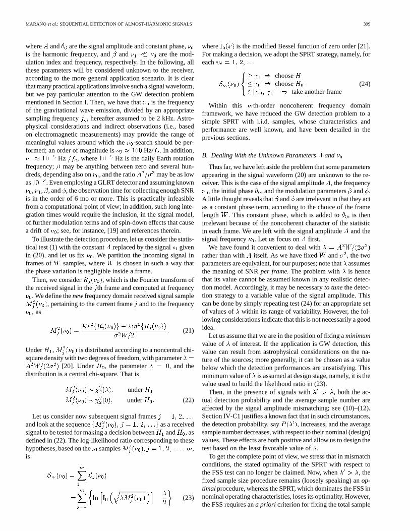
Fig. 2. Block diagram of the bank of sequential detectors. The DSP deviceprovides the spectral samplesM (� ) k = 1; 2; . . . ; Y (all the frequenciesof interest). These samples are then sent to individual branches, each tunedto a frequency value� , which compute the likelihood ratios; see (23). Thethreshold comparisons produce the local decisions or no decision at all. This isschematically denoted withD , wherem is the input data frame number andk the branch index. The last device takes the final decision on the basis ofD ,k = 1; 2; . . . ; Y , m = 1; 2; . . ..

number; this can be set on the basis of computational limits or,once again, on a minimum expected signal strength. The FSSultimately yields a detection probability gain ( ), al-though this may be of minor relevance if we are more interestedin minimizing the detection delay than in stressing the gain on

beyond the nominal and acceptable . (This dis-cussion is borrowed from [15]; see also [17, Sec. II]. Dealingwith SNRs that are different by that assumed at the design stageis a rather classical topic in sequential detection; see, for in-stance, [22].)

We now turn to the problem of the unknown signal frequency, which is considerably more problematic than. Within the

SPRT structure, there is no reasonable way to estimate the basicfrequency since such an estimate would require re-examinationof past data. The only reasonable approach seems to be to imple-ment a separate test for each different frequency. The frequencyaxis has to be properly discretized so that uniformly spaced fre-quency values are considered.

The detector structure takes the form of a bank of sequentialdetectors, each tuned to a frequency value. It is schemati-cally depicted in the block diagram of Fig. 2. On each branch

of the bank, apartial statistic isbuilt and, for each , compared with two thresholds (for sym-metry reasons these are the same on all the branches). Whena threshold is crossed, we say that apartial decisionhas beentaken, and the detection processon that branchstops.

The final decision is taken according to the following rules.

• A decision in favor of “signal presence” is taken at themoment thatany of the branch statisticscrosses its upperthreshold, namely, the first upper threshold crossing stopsthe detection process with final decision . In this case,the frequency pertaining to that branch is an estimate ofthe actual signal frequency.

Fig. 3. ASN versus detection probability withP = 10 and� = 0:3.Continuous curves refer to the designed SPRT detector, whereas dashed lines,which are depicted for comparison purposes, give the performance of them-noncoherent FSS. Points represent simulated values of SPRT. For clarity,the abscissa is plotted on a Gaussian scale.

• A decision in favor of “signal absence” is declared at themoment thatall of the branch statisticscross the respectivelower thresholds.

It is clear that the performance of the bank of sequential de-tectors depends on all the partial statistics, namely, on thelocalperformances of each of the individual branches. This is why,in the following section, we deal first with the simplified caseof a known value of (single branch) and then generalize theresults to the realistic case in which a search over theaxis hasto be performed (complete bank).

C. Performance of Proposed Noncoherent SPRT Bank

1) Performance With Known : In the case that the param-eters assumed at design stage, and, in particular, the value of,are exactly the same as those of the true incoming signal, thedetection and false alarm probabilities are equal to their nom-inal values and . The ASN can be derived on the basisof (7). The two density functions and to be considered are

and , respectively. The evaluation of the divergencein the denominator of (7) has been performed numerically andthe results, in terms of ASN under and , are shown inFig. 3 for , , as a function of plotted ona Gaussian scale. In this simulation, we refer to the case studyof , , and .

The points drawn in Fig. 3 represent simulated values andconfirm the accuracy of the analytical formulas. For the sake ofcomparison, we consider also a-order noncoherent FSS testthat achieves the same performance level. The correspondingfixed sample number is represented by the dashed lines of Fig. 3.We see, as expected, that the SPRT outperforms the FSS test, inthe sense that it requires, on average, fewer samples to come toa decision.

The situation is illustrated further in Fig. 4, where, along withthe ASN, we also provide, exploiting the formulas derived inSection II-B, the 10 and 90 percentiles of Wald’s distribution


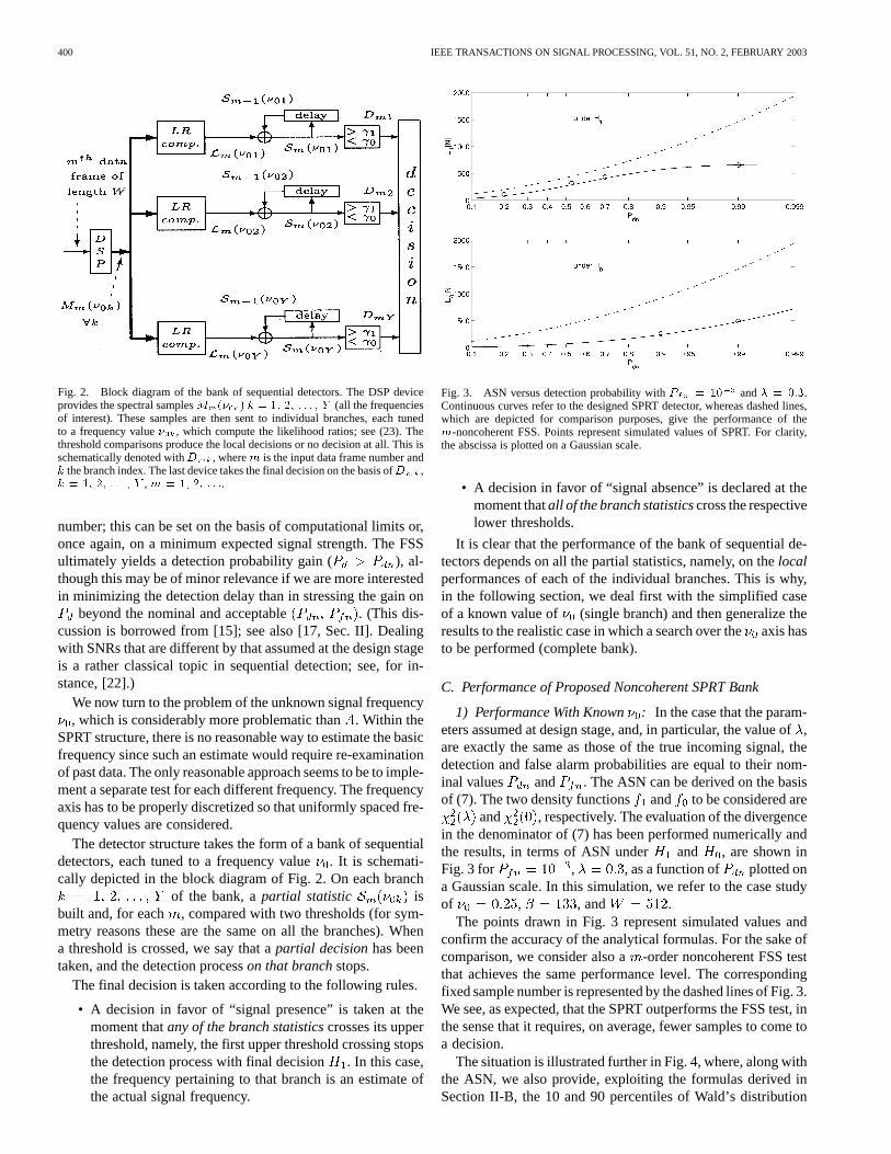
Fig. 4. Number of samples required to end the statistical test. Comparisonbetween the sequential procedure and an equivalentm-noncoherent FSS, withP = 10 for two different values of�. Continuous curves refer to theASN of the designed SPRT detector while dashed lines give the performance ofthe FSS. The two dash-and-dot curves refer to the 10 and 90 percentiles of theWald’s distribution.

that governs . It is worth noting that the sequential procedurerequires fewer samples than an FSS in at least 90% of the casesfor the performance values of interest.

Simpler formulas, which avoid the numerical integration in-volved in (7), can be obtained under the assumption of small.In fact, for vanishingly small , we can use the expansion [21]

(25)

which, neglecting the term in , yields. A discussion on the mismatch case is

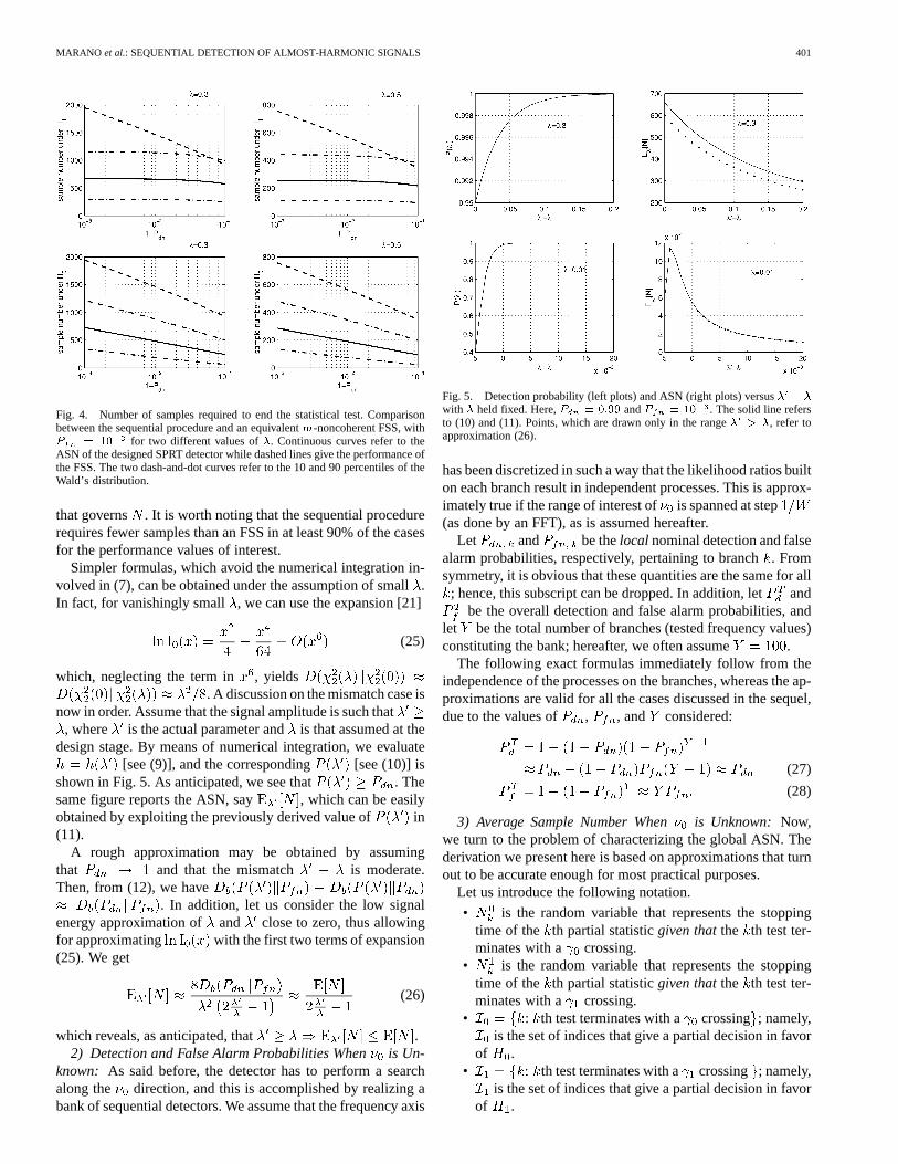
now in order. Assume that the signal amplitude is such that, where is the actual parameter andis that assumed at the

design stage. By means of numerical integration, we evaluate[see (9)], and the corresponding [see (10)] is

shown in Fig. 5. As anticipated, we see that . Thesame figure reports the ASN, say , which can be easilyobtained by exploiting the previously derived value of in(11).

A rough approximation may be obtained by assumingthat and that the mismatch is moderate.Then, from (12), we have

. In addition, let us consider the low signalenergy approximation of and close to zero, thus allowingfor approximating with the first two terms of expansion(25). We get

(26)

which reveals, as anticipated, that .2) Detection and False Alarm Probabilities Whenis Un-

known: As said before, the detector has to perform a searchalong the direction, and this is accomplished by realizing abank of sequential detectors. We assume that the frequency axis

Fig. 5. Detection probability (left plots) and ASN (right plots) versus� � �

with � held fixed. Here,P = 0:99 andP = 10 . The solid line refersto (10) and (11). Points, which are drawn only in the range� > �, refer toapproximation (26).

has been discretized in such a way that the likelihood ratios builton each branch result in independent processes. This is approx-imately true if the range of interest of is spanned at step(as done by an FFT), as is assumed hereafter.

Let and be thelocal nominal detection and falsealarm probabilities, respectively, pertaining to branch. Fromsymmetry, it is obvious that these quantities are the same for all

; hence, this subscript can be dropped. In addition, letandbe the overall detection and false alarm probabilities, and

let be the total number of branches (tested frequency values)constituting the bank; hereafter, we often assume .

The following exact formulas immediately follow from theindependence of the processes on the branches, whereas the ap-proximations are valid for all the cases discussed in the sequel,due to the values of , , and considered:

(27)

(28)

3) AverageSample Number When is Unknown: Now,we turn to the problem of characterizing the global ASN. Thederivation we present here is based on approximations that turnout to be accurate enough for most practical purposes.

Let us introduce the following notation.

• is the random variable that represents the stoppingtime of the th partial statisticgiven thatthe th test ter-minates with a crossing.

• is the random variable that represents the stoppingtime of the th partial statisticgiven thatthe th test ter-minates with a crossing.

• : th test terminates with a crossing ; namely,is the set of indices that give a partial decision in favor

of .• th test terminates with a crossing ; namely,

is the set of indices that give a partial decision in favorof .


• .• is the random variable denoting the stopping time of

the global test running on the filterbank.• is the index for the filter perfectly matched to the in-

coming signal under .Let us focus on hypothesis first. We get

is chosen

is chosen (29)

Since is close to unity, the first term can be neglected. Ac-cordingly, we have

is chosen

is nonempty

(30)

The approximation is to assume that the single local statistic la-beled with crosses the upper threshold in hypothesis .Namely, we assume that the cardinality of, which is expectedto be of few units, is just one and the index is just the right index

. The distribution of the can be approximated by the dis-tribution of the unconditioned stopping time because, under

, the lower threshold crossing is a rare event (an approxima-tion similar to the single-threshold assumption yielding Wald’sdistribution for ). Thus, we end up with the simple formula

under (31)

When the hypothesis in force is , in a similar fashion, we get

is chosen

The latter approximation amounts to replacement of the con-ditioned variables by the unconditioned counterparts ,

. Notice that the assumptions stated at the be-ginning of Section IV-C2 imply that are i.i.d.under . Then, by exploiting Wald’s distribution, we finallyget under

(32)Formulas (31) and (32) have been checked by simulations,

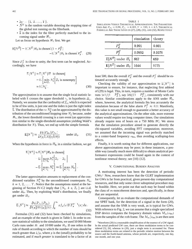
and an example of the match is given in Table I. In order to en-sure statistical validity to the simulations, we used 50 000 MonteCarlo runs under and 10 000 under . If one refers to therule of thumb according to which the number of runs should bemuch greater than , where is the (small) probability to beestimated, and ifmuch greateris translated to be a factor of at

TABLE ISIMULATIONS VERSUSTHEORETICAL APPROXIMATIONS. THE PARAMETERS

USED AREP = 0:99, P = 0:001, Y = 100, � = 0:3. THEORETICAL

FORMULAS ARE THOSEGIVEN IN (27), (28), (31),AND (32), RESPECTIVELY

least 500, then the overall and the overall should be es-timated accurately enough.

Checking the validity of our approximation to isimportant to ensure, for instance, that neglecting first addendof (29) is legal. This, in turn, requires a number of Monte Carloruns , say , consistently with ourchoice. Similar considerations apply to the ANS under,where, however, the analytical formula fits less accurately thesimulation because of the false alarm : Manifestly,this value is not small enough to guarantee a better accuracy ofthe analytical approximations. On the other side, more extremevalues would require too long computer times. Our simulationsalready require tens of hours on a 750 MHz PC. We stressthat the simulation procedure aimed to generate directly thechi-squared variables, avoiding FFT computation; moreover,we assumed that the incoming signal was perfectly matchedto a center-band frequency , thus avoiding scalloping-losseffects.

Finally, it is worth noting that for different applications, ourabove approximations may be poor; in these instances, a pos-sible way (usually much more difficult) to obtain analytical per-formance expressions could be found again in the context ofnonlinear renewal theory; see [10]–[12].

V. COMPUTATIONAL BURDEN ANALYSIS

A motivating interest has been the detection of periodicGWs.2 Now, researchers know that the GLRT implementationfor GWs is far from practical, given present-day computationalresources, and that only some clever suboptimal procedure maybe feasible. Here, we point out that such may be found withinthe class of -noncoherent detectors and, specifically, in thosethat are sequential.

Consequently, let us evaluate the computational demands ofour SPRT bank, for the detection of a signal in the form (20),and assume that the SNR is very weak, as is typical for GWs.With reference to Fig. 2, we can assume that a single specializedDSP device computes the frequency domain valuesfrom the samples of the th frame. The s are then sent

2Waveform (20) is a reasonable simplification of the essence of a GW signal.In the actual predicted GW case, there are three modulation terms to be con-sidered [5], [6], whereas in (20), just a single term is accounted for. Thesethree modulation terms are related to the periodic relative motion between thesource and the Earth-based antenna, whose periods are, respectively, one day,one month, and one year.


to individual computational units: one for each value of ,and these evaluate the test statistics; see (23). We neglect thecomputational costs associated with the statistic computationon each branch, focusing on the DSP burden. The DSP devicemay implement an FFT algorithm, which requiresfloating operations (FLOPs), providing all the DFT samples;actually, we are interested in a-search over a set of values,and may be much less than . In this case, it is convenient toresort to the so-called zoom-FFT algorithm, whose complexityis in the order of operations [23]. Furthermore, in thesequential case, the number of filters of the bank that areactive (no decision taken) at a certain timeis attime 0 but rapidly decreases in time. If , a directevaluation of the DFT that requires FLOPs via, e.g.,the Goertzel algorithm exploiting a recursive filtering of the data[24], may be convenient.

Thus, resorting to zoom-FFT algorithms, if ,and to direct DFT evaluation otherwise, we get the average com-putational complexity pertaining to the SPRT bank as

Pr

Pr (33)

where

(34)

with .Note that in the assumption that at best a single useful signal

is embedded in the noisy data, all (except maybe one) filterswork on noise-only samples; accordingly, the probability massfunction of can be computed by using Wald’s distribution(15) with parameters computed under; see Section II-B. Weget

Pr

(35)

Fig. 6 shows the behavior of for various data recordblock sizes . A smaller is of course simpler to implement;unfortunately, a smaller also increases the observationtime required to meet the specified and . For com-parison purposes, the computational burden associated to thefixed-sample-size bank is also given. The advantage of theSPRT—over the FSS—bank is quite evident, and it is inter-esting that it appears to increase as thebecomes smaller.

Apart from the computational costs, there is another valuablebenefit in using the sequential approach: The number ofcan-didate frequenciesdecreases with time since many frequenciesare ruled out. From a practical point of view, GW detection ismuch simpler if the signal frequency is known or if the numberof candidate frequencies is limited to few units so that whenthe number of surviving branches is small enough, one of the

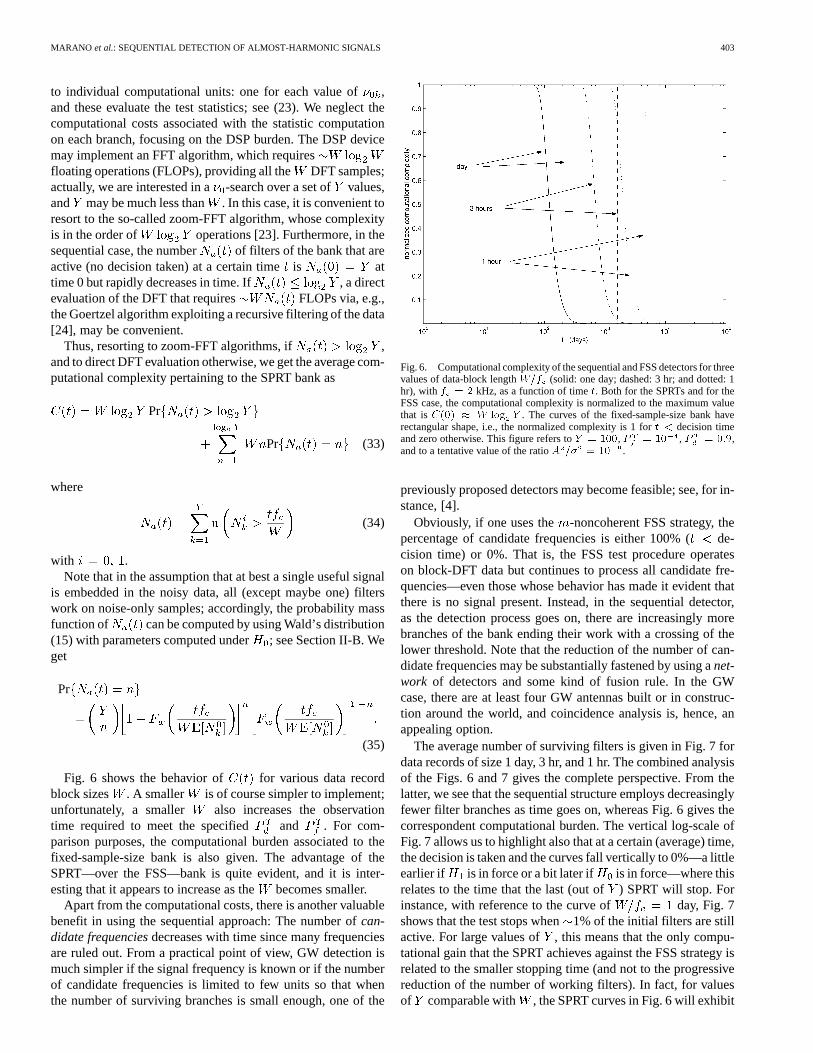
Fig. 6. Computational complexity of the sequential and FSS detectors for threevalues of data-block lengthW=f (solid: one day; dashed: 3 hr; and dotted: 1hr), with f = 2 kHz, as a function of timet. Both for the SPRTs and for theFSS case, the computational complexity is normalized to the maximum valuethat isC(0) � W log Y . The curves of the fixed-sample-size bank haverectangular shape, i.e., the normalized complexity is 1 fort < decision timeand zero otherwise. This figure refers toY = 100, P = 10 , P = 0:9,and to a tentative value of the ratioA =� = 10 .

previously proposed detectors may become feasible; see, for in-stance, [4].

Obviously, if one uses the -noncoherent FSS strategy, thepercentage of candidate frequencies is either 100% (de-cision time) or 0%. That is, the FSS test procedure operateson block-DFT data but continues to process all candidate fre-quencies—even those whose behavior has made it evident thatthere is no signal present. Instead, in the sequential detector,as the detection process goes on, there are increasingly morebranches of the bank ending their work with a crossing of thelower threshold. Note that the reduction of the number of can-didate frequencies may be substantially fastened by using anet-work of detectors and some kind of fusion rule. In the GWcase, there are at least four GW antennas built or in construc-tion around the world, and coincidence analysis is, hence, anappealing option.

The average number of surviving filters is given in Fig. 7 fordata records of size 1 day, 3 hr, and 1 hr. The combined analysisof the Figs. 6 and 7 gives the complete perspective. From thelatter, we see that the sequential structure employs decreasinglyfewer filter branches as time goes on, whereas Fig. 6 gives thecorrespondent computational burden. The vertical log-scale ofFig. 7 allows us to highlight also that at a certain (average) time,the decision is taken and the curves fall vertically to 0%—a littleearlier if is in force or a bit later if is in force—where thisrelates to the time that the last (out of) SPRT will stop. Forinstance, with reference to the curve of day, Fig. 7shows that the test stops when1% of the initial filters are stillactive. For large values of , this means that the only compu-tational gain that the SPRT achieves against the FSS strategy isrelated to the smaller stopping time (and not to the progressivereduction of the number of working filters). In fact, for valuesof comparable with , the SPRT curves in Fig. 6 will exhibit


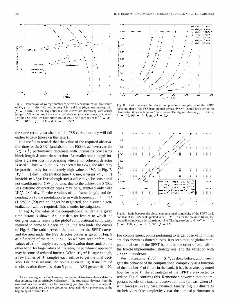
Fig. 7. Percentage of average number of active filters at timet for three valuesof W=f = 1 day (leftmost curves), 3 hr, and 1 hr (rightmost curves), withf = 2 kHz. For the sequential test, the curves are decreasing with abruptjumps to 0% at the time instant of a final decision (average values, of course).For the FSS case, we have either 100 or 0%. The figure refers toY = 100,P = 10 , P = 0:9, andA =� = 10 .

the same rectangular shape of the FSS curve, but they will fallearlier to zero (more on this later).

It is useful to remark that the value of the required observa-tion time for the SPRT (and also for the FSS) to achieve a certain

) performance decreases with increasing processingblock-length since the selection of a smaller block-length im-plies a greater loss in processing when a noncoherent detectoris used.3 Thus, with the SNR expected for GWs, the idea maybe practical only for moderately high values of. In Fig. 7,

day observation time 6 mo, whereashr yields 3.5 yr. Even though such a value might be considerednot exorbitant for GW problems, due to the achievable SNRs,less extreme observation times may be guaranteed only with

day. For these values of the frame length, and de-pending on , the modulation term with frequency(1 day) in (20) can no longer be neglected, and a suitable gen-eralization will be required. This is under investigation.

In Fig. 6, the value of the computational burden at a giventime instant is shown. Another detector feature to which thedesigner usually refers is theglobal computational complexityrequired to come to a decision, i.e., the area under the curvesof Fig. 6. The ratio between the area under the SPRT curvesand the area under the FSS detector curves is given in Fig. 8as a function of the ratio . As we have seen before, lowvalues of imply very long observation times and, on theother hand, for large values of this ratio, the partitioned approachmay become of reduced interest. When is large enough,a few frames of samples each suffice to get the final deci-sion. For these reasons, the points given in Fig. 8 are limitedto observation times less than 5 yr and to ASN greater than 20.

3As we have argued before, however, this loss is relative to a coherent detectorthat assumes, not surprisingly, coherence. If the true signal deviates from theassumed coherent model, then the processinggain from the use of a largeWmay be fallacious; see also the discussion about spin-down phenomena at thebeginning of Section IV-A.

Fig. 8. Ratio between the global computational complexity of the SPRTbank and that of the FSS bank plotted versusA =� . Dotted lines pertain toobservation times as large as 5 yr or more. The figure refers tof = 2 kHz,Y = 100, P = 10 , andP = 0:9.

Fig. 9. Ratio between the global computational complexity of the SPRT bankand that of the FSS bank, plotted versusY=W . As for the previous figure, thedotted lines indicate a decision time> 5 yr. The figure refers toA =� = 10 ,f = 2 kHz,P = 10 , andP = 0:9.

For completeness, points pertaining to larger observation timesare also shown as dotted curves. It is seen that the global com-putational cost of the SPRT bank is in the order of one half ofthe fixed-sample-number strategy one, and the variation with

is moderate.We now assume , as done before, and investi-

gate the behavior of the computational complexity as a functionof the number of filters in the bank. It has been already notedhow for large , the advantages of the SPRT are expected toreduce. Fig. 9 confirms this. Remember, however, that the im-portant benefit of a smaller observation time (at least whenis in force) is, in any case, retained. Finally, Fig. 10 illustratesthe behavior of the complexity versus the nominal performances


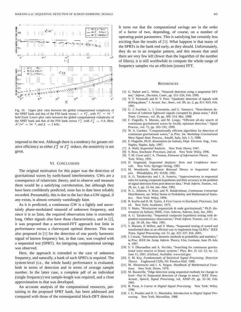
Fig. 10. Upper plot: ratio between the global computational complexity ofthe SPRT bank and that of the FSS bank versus1 � P , with P = 10

held fixed. Lower plot: ratio between the global computational complexity ofthe SPRT bank and that of the FSS bank versusP with P = 0:9. Here,A =� = 10 , andf = 2 kHz.

imposed to the test. Although there is a tendency for greater rel-ative efficiency as either or reduce, the sensitivity is notgreat.

VI. CONCLUSIONS

The original motivation for this paper was the detection ofgravitational waves by earth-based interferometry. GWs are aconsequence of relativistic theory, and to observe and measurethem would be a satisfying corroboration, but although theyhave been confidently predicted, none has to date been reliablyrecorded. Presumably, this is due to the fact that a GW signal, ifany exists, is almost certainly vanishingly faint.

As it is predicted, a continuous GW is a lightly and uncer-tainly phase-modulated sinusoid of unknown frequency, andsince it is so faint, the required observation time is extremelylong. Other signals also have these characteristics, and in [2],it was proposed that a sectioned-FFT approach lost little inperformance versus a clairvoyant optimal detector. This wasalso proposed in [1] for the detection of one purely harmonicsignal of known frequency but, in that case, was coupled witha sequential test (SPRT). An intriguing computational savingswas observed.

Here, the approach is extended to the case of unknownfrequency, and naturally, a bank of such SPRTs is required. Thesystem-level (i.e., the whole bank) performance is evaluated,both in terms of detection and in terms of average samplenumber. In the latter case, a complete pdf of an individual(single frequency) test sample-length was required, and a closeapproximation to that was developed.

An accurate analysis of the computational resources, per-taining to the proposed SPRT bank, has been addressed andcompared with those of the nonsequential block-DFT detector.

It turns out that the computational savings are in the orderof a factor of two, depending, of course, on a number ofoperating-point parameters. This is satisfying but certainly lessexciting than the results of [1]. What happens is that many ofthe SPRTs in the bank end early, as they should. Unfortunately,they do so in an irregular pattern, and this means that untilthere are very few left (fewer than the logarithm of the numberof filters), it is still worthwhile to compute the whole range offrequency samples via an efficient (zoom) FFT.

REFERENCES

[1] G. Parker and L. White, “Sinusoid detection using a sequential DFTtest,” Inform., Decision, Contr., pp. 551–556, Feb. 1999.

[2] V. V. Veeravalli and H. V. Poor, “Quadratic detection of signals withdrifting phase,”J. Acoust. Soc. Amer., vol. 89, no. 2, pp. 811–819, Feb.1991.

[3] G. J. Foschini, L. J. Greenstein, and G. Vannucci, “Noncoherent de-tection of coherent lightwave signals corrupted by phase noise,”IEEETrans. Commun., vol. 36, pp. 306–314, Mar. 1988.

[4] F. Flagiello, S. Marano, and M. Longo, “Efficient all-sky search ofcontinuous gravitational waves by locally optimum detection,”SignalProcess., vol. 72, pp. 183–192, 1999.

[5] W. A. Gardner, “Computationally efficient algorithms for detection ofcontinuous gravitational waves,” inProc. Int. Workshop GravitationalWave Signal Anal. Process., Amalfi, Italy, July 1–5, 1988.

[6] F. Flagiello, Ph.D. dissertation (in Italian), Dept. Electron. Eng., Univ.Naples, Naples, Italy, 1997.

[7] A. Wald, Sequential Analysis. New York: Dover, 1947.[8] S. Ross,Stochastic Processes, 2nd ed. New York: Wiley, 1996.[9] T. M. Cover and J. A. Thomas,Elements of Information Theory. New

York: Wiley, 1991.[10] D. Siegmund, Sequential Analysis: Tests and Confidence Inter-

vals. New York: Springer-Verlag, 1985.[11] M. Woodroofe, Nonlinear Renewal Theory in Sequential Anal-

ysis. Philadelphia, PA: SIAM, 1982.[12] A. G. Tartakovsky and I. A. Ivanova, “Approximations in sequential

rules for testing composite hypotheses and their accuracy in the problemof signal detection from post-detector data,”Prob. Inform. Transm., vol.28, no. 1, pp. 55–64, Jan.–Mar. 1992.

[13] N. L. Johnson, S. Kotz, and N. Balakrishnan,Continuous UnivariateDistributions, ser. Wiley Series in Probability and Mathematical Statis-tics. New York: Wiley, 1994.

[14] R. Karlin and H. M. Taylor,A First Course in Stochastic Processes, 2nded. New York: Academic, 1975.

[15] V. Matta, “Rivelazione sequenziale di onde gravitazionali,” Ph.D. dis-sertation (in Italian), DIIIE, Univ. Salerno, Salerno, Italy, Jan. 2001.

[16] A. G. Tartakovsky, “Sequential composite hypothesis testing with de-pendent nonstationary observations,”Prob. Inform. Transm., vol. 17, no.1, pp. 18–28, Jan.–Mar. 1981.

[17] S. Marano, P. Willett, and V. Matta, “Sequential testing of sorted andtransformed data as an efficient way to implement long GLRTs,”IEEETrans. Signal Processing, vol. 51, pp. 325–337, Feb. 2003.

[18] I. Csiszár, “Information theoretic methods in probability and statistics,”in Proc. IEEE Int. Symp. Inform. Theory, Ulm, Germany, June 29–July4, 1997.

[19] S. V. Dhurandhar and A. Vecchio, “Searching for continuous gravita-tional wave sources in binary systems,”Phys. Rev. D, vol. 63, no. 12,June 15, 2001. [Online]. Available: www.lanl.gov.

[20] S. M. Kay, Fundamentals of Statistical Signal Processing: DetectionTheory. Englewood Cliffs, NJ: Prentice-Hall, 1988.

[21] M. Abramowitz and I. A. Stegun,Handbook of Mathematical Func-tions. New York: Dover, 1970.

[22] M. Basseville, “Edge detection using sequential methods for change inlevel—Part II: Sequential detection of change in mean,”IEEE Trans.Acoust., Speech, Signal Processing, vol. ASSP–29, pp. 32–50, Feb.1981.

[23] B. Porat,A Course in Digital Signal Processing. New York: Wiley,1996.

[24] J. G. Proakis and D. G. Manolakis,Introduction to Digital Signal Pro-cessing. New York: Macmillan, 1988.


Stefano Maranoreceived the Laurea degree in elec-tronic engineering (cum laude) and the Ph.D. degreein electronic engineering and computer science, bothfrom the University of Naples, Naples, Italy, in 1993and 1997, respectively.

In November 1999, he was appointed the perma-nent position of Assistant Professor at the Universityof Salerno, Fisciano, Italy. His current research in-terests include detection and estimation theory, withemphasis on sequential detection procedures andreal-data analysis; decentralized fusion; stochastic

modeling of electromagnetic propagation in random media; and internettomography. He serves as referee for the main international journals publishingin the field of signal processing.

Dr. Marano was the co-recipient of the S. A. Schelkunoff Transactions PrizePaper Award of the IEEE Antennas and Propagation Society for the best paperpublished in the IEEE TRANSACTIONS ON ANTENNAS AND PROPAGATION in1999.

Vincenzo Matta received the Laurea degree (cumlaude) in electronic engineering from Universityof Salerno, Fisciano, Italy, in 2001, where he iscurrently pursuing the Ph.D. degree in informationengineering.

His main research interests include detection andestimation theory, with emphasis on sequential de-tection procedures and real-data analysis; detectionof gravitational waves; and internet tomography.

Peter Willett (SM’97) received the B.A.Sc.degree from the University of Toronto, Toronto,ON, Canada, in 1982 and the Ph.D. degree fromPrinceton University, Princeton, NJ, in 1986.

He is a Professor of electrical and computerengineering at the University of Connecticut,Storrs. He has written, among other topics, aboutthe processing of signals from volumetric arrays,decentralized detection, information theory, codedivision multiple access, learning from data, targettracking, and transient detection.

Dr. Willett is a Member of the IEEE Signal Processing Society’s Sensor Arrayand Multichannel Technical Committee. He is an associate editor both for theIEEE TRANSACTIONS ONAEROSPACE ANDELECTRONIC SYSTEMS and for theIEEE TRANSACTIONS ONSYSTEMS, MAN, AND CYBERNETICS. He is a track or-ganizer for Remote Sensing at the IEEE Aerospace Conference (2001–2003)and is co-chair of the Diagnostics, Prognosis, and System Health ManagementSPIE Conference in Orlando, FL.

Sequential detection of almost-harmonic signals - … · Sequential Detection of Almost-Harmonic...

Documents

Transcript of Sequential detection of almost-harmonic signals - … · Sequential Detection of Almost-Harmonic...