Rose-Hulman Institute of TechnologyRose-Hulman ScholarGraduate Theses - Electrical and ComputerEngineering Graduate Theses

5-2018

Harmonic Detection and Selectively FocusingElectromagnetic Waves onto Nonlinear Targetsusing Time-ReversalJoseph Michael Faia

Follow this and additional works at: https://scholar.rose-hulman.edu/electrical_grad_theses

Part of the Electrical and Computer Engineering Commons

This Thesis is brought to you for free and open access by the Graduate Theses at Rose-Hulman Scholar. It has been accepted for inclusion in GraduateTheses - Electrical and Computer Engineering by an authorized administrator of Rose-Hulman Scholar. For more information, please contactweir1@rose-hulman.edu.

Recommended CitationFaia, Joseph Michael, "Harmonic Detection and Selectively Focusing Electromagnetic Waves onto Nonlinear Targets using Time-Reversal" (2018). Graduate Theses - Electrical and Computer Engineering. 10.https://scholar.rose-hulman.edu/electrical_grad_theses/10

Harmonic Detection and Selectively Focusing Electromagnetic Waves onto Nonlinear Targets using Time-Reversal

A Thesis

Submitted to the Faculty

of

Rose-Hulman Institute of Technology

By

Joseph Michael Faia

In Partial Fulfillment of the Requirements for the Degree of Master

of

Science in Electrical Engineering

May 2018

© 2018 Joseph Michael Faia

i

ABSTRACT

Faia, Joseph Michael

M.S.E.E.

Rose-Hulman Institute of Technology

May 2018

Harmonic Detection and Selectively Focusing Electromagnetic Waves onto Nonlinear Targets using

Time-Reversal

Thesis Advisor: Dr. Edward Wheeler

Ultra-wide band radar is a growing interest for the enhanced capability of ranging, imaging,

and multipath propagation. An ultra-wide band pulse imposed on a system provides a near impulse

like response and is, therefore, more descriptive than a conventional monotonic pulse. Combining

pulse inversion with ultra-wide band DORT (a French acronym for the decomposition of the time

reversal operator) is a technique which could be used to for greater visibility of nonlinear targets

via harmonic detection in the presence of larger linear scatterers. Energy can be selectively focused

onto nonlinear scatterers in complex, inhomogeneous environments. This thesis1, will expand

upon previous work, and demonstrate nonlinear detection and selective focusing with pulse

inversion combined with DORT.

1 This thesis builds on conference paper published and presented at URSI GASS 2017 in Montreal,

Canada and forms the basis for a journal paper to be submitted this Spring.

ii

DEDICATION

This thesis is dedicated to my parents Dan and Dawn Faia for their unwavering love and support.

Thank you for providing the opportunity and encouragement to pursue my education in Electrical Engineering

iii

ACKNOWLEDGEMENTS

This thesis would not have been possible without the guidance and expertise brought by

Dr. Sun Hong. I would like to thank him for introducing me to this project and working with me.

I would also like to thank Dr. Ed Wheeler for his support of the work in this thesis. I would like to

thank Yuije “Tao” He and Matthew Howlett who were huge contributors in the setup of the

experiment and development of the experimental procedure. Finally, I owe a lot to the ECE

Department technicians Jack Shrader, Garry Meyers, and Mark Crosby for their time and efforts

in ensuring that we had everything we needed for this investigation.

iv

TABLE OF CONTENTS

TABLE OF FIGURES ............................................................................................................................... vi

LIST OF ABBREVIATIONS ................................................................................................................... ix

LIST OF SYMBOLS .................................................................................................................................. x

GLOSSARY................................................................................................................................................ xi

1. INTRODUCTION ............................................................................................................................... 1

2. BACKGROUND ................................................................................................................................. 3

Time-Reversal Invariance of the Lossless Wave Equation ....................................................................... 3

Generated Harmonics of Nonlinear Systems ............................................................................................ 4

3. LITERATURE REVIEW................................................................................................................... 6

Time-Reversal Mirror ............................................................................................................................... 6

The DORT Method ................................................................................................................................... 7

Pulse Inversion ........................................................................................................................................ 10

Nonlinear Time-Reversal ........................................................................................................................ 11

4. SIMULATED PI-DORT................................................................................................................... 13

Method .................................................................................................................................................... 13

Results ..................................................................................................................................................... 14

One Linear and One Nonlinear .......................................................................................................... 14

Two Nonlinear .................................................................................................................................... 18

Discussion ............................................................................................................................................... 19

5. DESCRIPTION OF MODEL .......................................................................................................... 20

Vivaldi Antenna ...................................................................................................................................... 20

Antenna Array ......................................................................................................................................... 23

Distributed Antenna Network ................................................................................................................. 25

Linear Target ........................................................................................................................................... 25

Nonlinear Target ..................................................................................................................................... 26

Interrogation Pulse .................................................................................................................................. 27

DORT Processing Script ......................................................................................................................... 28

Experimental Procedure .......................................................................................................................... 30

6. EXPERIMENTAL PI-DORT .......................................................................................................... 47

Method .................................................................................................................................................... 47

Results ..................................................................................................................................................... 48

One Linear Target ............................................................................................................................... 48

One Nonlinear Target ......................................................................................................................... 49

v

One Linear and One Nonlinear Target ............................................................................................... 51

Discussion ............................................................................................................................................... 53

7. FUTURE WORK .............................................................................................................................. 54

Addressing the Eigenvalue mixing problem ........................................................................................... 54

Furthering performance with Improved Antenna Design ....................................................................... 55

Frequency Signatures .............................................................................................................................. 55

Potential Applications ............................................................................................................................. 56

8. Survey of Applications ...................................................................................................................... 57

Biomedical Imaging and Microwave Thermotherapy ............................................................................ 57

Wireless Power Transfer ......................................................................................................................... 57

Security and Defense .............................................................................................................................. 58

5G Communications and IoT .................................................................................................................. 58

9. CONCLUSION ................................................................................................................................. 59

REFERENCES .......................................................................................................................................... 60

APPENDICES ........................................................................................................................................... 62

APPENDIX A—Pulse Generation Script ............................................................................................... 63

APPENDIX B –PI -DORT Processing Script ......................................................................................... 65

APPENDIX C—Spatially Variant Lens Paper Sent for Submission ................................................... 69

vi

TABLE OF FIGURES

Figure 1.1: Timeline for the Development of PI-DORT ............................................................................. 2

Figure 2.1: Illustration of the response of a (a) linear system, (b) asymmetric distortion nonlinear system and (c) symmetric distortion nonlinear system ............................................................................................. 4

Figure 3.1: Illustration of the TRM process of focusing to a point scatterer (a) the environment is interrogated with a short pulse (b) the scattered response suggests a complex medium and (c) the signal is mirrored in time and re-transmitted to reconstruct the pulse at the target .................................................... 7

Figure 3.2: Multi-static data matrix in (a) time domain and (b) frequency domain .................................... 8

Figure 3.3: Eigenvalue Decomposition of TRO Matrix ............................................................................... 9

Figure 4.1: PI-DORT simulation domain (a) first configuration with one linear and one nonlinear target (b) second configuration with two nonlinear targets................................................................................... 13

Figure 4.2: DORT using background subtraction for 1L and 1NL target .................................................. 15

Figure 4.3: Simulated focusing results for (a) the first eigenvalue (λ1) and (b) the second eigenvalue (λ2) .................................................................................................................................................................... 15

Figure 4.4: PI-DORT eigenvalues for 1L and 1NL target ......................................................................... 17

Figure 4.5: PI-DORT focusing onto 1NL target ........................................................................................ 17

Figure 4.6: Eigenvalues for 2NL targets .................................................................................................... 18

Figure 4.7: Focusing for 2NL targets with (a) eigenvalue 1 and (b) eigenvalue 2 .................................... 19

Figure 5.1: Electric Field lines on a Vivaldi antenna ................................................................................. 21

Figure 5.2: CST Model of Vivaldi Antenna .............................................................................................. 21

Figure 5.3: Measured and Simulated Return Loss for two Vivaldi antennas ............................................ 22

Figure 5.4: Usable Gain Bandwidth measurement setup ........................................................................... 22

Figure 5.5: Usable Gain Bandwidth for Vivaldi antennas ......................................................................... 23

Figure 5.6: Illustration of the Fraunhofer approximation in an array ........................................................ 24

Figure 5.7: Metal sphere suspended in interrogation environment ............................................................ 25

Figure 5.8: Simulated RCS pattern of a PEC sphere ................................................................................. 26

Figure 5.9: Bowtie antenna for NL targets ................................................................................................ 26

vii

Figure 5.10: Bowtie Antenna for NL Targets (a) Scattering Pattern at 3 GHz and (b) radiation pattern at 6 GHz ............................................................................................................................................................. 27

Figure 5.11: Interrogation Pulse ................................................................................................................ 27

Figure 5.12: Data Import matrix in the time-domain ................................................................................. 28

Figure 5.13: Data-Import matrix in the frequency domain ........................................................................ 28

Figure 5.14: multi-static matrix unarranged .............................................................................................. 29

Figure 5.15: Multi-static data matrix in time domain ............................................................................... 29

Figure 5.16: Workflow diagram for DORT experiment ............................................................................ 30

Figure 5.17: Benchtop Instrumentation for Experiment ............................................................................ 31

Figure 5.18: Demonstration of grating lobes with spacing (a) at 10 cm and (b) at 5 cm ........................... 32

Figure 5.19: Initial Experimental Setup ..................................................................................................... 33

Figure 5.20: Initial DORT results: one linear target .................................................................................. 34

Figure 5.21: Initial bi-static result one linear target (a) raw measurement (b) background subtracted ..... 35

Figure 5.22: Relative path length differences ............................................................................................ 36

Figure 5.23: Second Experimental Setup (a) Functional Diagram (b) Anechoic Chamber Photo ............. 37

Figure 5.24: Second Experimental results ................................................................................................. 38

Figure 5.25: Second Experimental results linear scaling ........................................................................... 39

Figure 5.26: Initial bi-static result one linear target (a) raw measurement (b) background subtracted...... 39

Figure 5.27: Second Experimental results linear scaling after time-gating ............................................... 40

Figure 5.28: NL Experimental setup .......................................................................................................... 41

Figure 5.29: NL Bi-static test (a) time domain and (b) frequency domain ................................................ 41

Figure 5.30: Nonlinear Experimental results in linear scaling ................................................................... 42

Figure 5.31: Nonlinear Experimental Bi-Static Time Domain .................................................................. 43

Figure 5.32: Nonlinear Experimental Mono-Static Time Domain ............................................................ 43

Figure 5.33: NL Experiment Setup ............................................................................................................ 44

Figure 5.34: Nonlinear Experimental results in linear scaling ................................................................... 44

viii

Figure 5.35: Quasi-mono-static measurement ........................................................................................... 45

Figure 5.36: Nonlinear Experimental results in linear scaling ................................................................... 46

Figure 6.1: Eigenvalues and eigenvectors from one linear target. ............................................................. 48

Figure 6.2: Eigenvalues and eigenvectors from one linear target. ............................................................. 49

Figure 6.3: Eigenvalue and Eigenvector for off-centered diode using a closely spaced array .................. 50

Figure 6.4: One linear and One NL experimental setup, diode is on the left and linear target is on the right ............................................................................................................................................................. 51

Figure 6.5: One Linear and One Nonlinear Target using Background subtraction eigenvalues ................ 52

Figure 6.6: One Linear and One Nonlinear Target using PI-DORT .......................................................... 52

ix

LIST OF ABBREVIATIONS

TR Time-reversal

TRM Time-reversal mirror

NL Nonlinear

PI Pulse inversion

DORT French acronym for decomposition of the time-reversal operator

EM Electromagnetic

EVD Eigenvalue decomposition

SVD Singular value decomposition

TRO Time-reversal operator

MDS Minimum discernable signal

DNR Dynamic range

UWB Ultra-wide band

VNA Vector network analyzer

CST MWS Computer Simulation Technology – Microwave Studio®

RF Radio frequency

x

LIST OF SYMBOLS

English symbols

𝑬𝑬 Electric field vector in the electromagnetic wave equation

𝑴𝑴 Multi-static data matrix

𝑯𝑯 Transfer matrix

𝑓𝑓 Frequency (in Hertz)

𝑡𝑡 Time (in seconds)

𝑚𝑚 Meters

𝑙𝑙 Path length

𝑑𝑑 Array spacing

Greek Symbols

𝜆𝜆 Wavelength

𝜔𝜔 Frequency (in radians per second)

𝜀𝜀 Permittivity of the medium

𝜇𝜇 Permeability of the medium

𝜑𝜑 Angle of target off of the normal vector of the array

xi

GLOSSARY

Harmonics Spectral copies of frequency response, occurs at integer multiples of the fundamental frequency

Time-reversal The response of the data y(t) has a time-reversal response of y(-t)

Multi-static The dataset which consists of a matrix containing all possible mono-static and bi-static combinations

Mono-static The dataset in which the transmit and receive antenna are the same

Bi-static The dataset in which the transmit and receive antenna are different

Greens function Describes the impulse response of a system in both space and time

Eigenvalues Scalar values that are characteristic to a set of differential equations

Eigenvectors A vector that when operated on by a given operator gives a scalar multiple of itself

1

1. INTRODUCTION

Developing the means to more efficiently and effectively detect and locate targets of

interest using electromagnetic waves has important applications ranging from wireless power

transfer to cancer detection to threat identification, all of which become significantly more difficult

in an inhomogeneous environment. In the work reported here, techniques originally developed for

use in acoustics are adapted to detect targets acting as non-linear scatterers of electromagnetic

waves.

In the early 1990’s, Mathias Fink from the University of Paris developed a technique using

time-reversal (TR) which allows a broadband signal from an acoustic point source to be detected

by an array of sensors, for this received signal to then be modified via TR to create a signal to be

fed back as the excitation to the acoustic array which results in a signal which focuses at the

location of the original point source, thereby allowing the acoustic array to act as a time-reversal

mirror (TRM) [1].

The next stage of refinement was realized when the array was allowed to act as original

excitation with the scattered signal from a target serving the role of point source. This was a crucial

step in that it allowed Fink’s PhD student Claire Prada to use the array as excitation to multiple

targets which then act as multiple scatterers. Together Prada and Fink developed a powerful

technique allowing for selective focusing on multiple targets, a technique known as decomposition

of the time-reversal operator (known as DORT after the French acronym) [2]. Since all this work

ultimately rests on the fact that acoustic waves are governed by the wave equation, these techniques

originally developed for acoustics can also be used in investigations involving electromagnetic

(EM) waves [3].

2

Figure 1.1: Timeline for the Development of PI-DORT

In this report, DORT is used in the identification of targets which scatter EM waves,

specifically on targets having non-linear (NL) characteristics such as diodes and transistors which

scatter waves with harmonics of the excitation frequencies. The main obstacle in attempting to

detect such NL targets in a complex environment of linear clutter (e.g., furniture, trees, and

buildings) is that the NL signals, particularly the harmonic responses, are often orders of

magnitude smaller than the waves scattered from linear targets. It is shown that summing the

responses from two broadband time-domain pulses, with one an inverted version of the other,

results in the odd-order harmonics, including the fundamental, to be largely removed while at the

same time enhancing the even-order harmonics. The aim of this work is to show that using DORT

together with pulse inversion (PI) allows relatively small nonlinear targets to be distinguished in a

complex environment, even one involving much larger linear targets [4].

The work presented in this thesis combines the use of ultra-wide band DORT and PI to

detect and selectively focus on NL targets in complex propagation environments. The simulation

and experimental results presented in this thesis provide substantial validation of PI DORT theory

with potential applications in defense, medicine, security, wireless power transfer and

communications.

3

2. BACKGROUND

Using conventional radar techniques it can be difficult to detect and focus energy onto a

target in an inhomogeneous (complex) environment. It would be an important step if this difficulty

could be overcome since, in many real-world applications, the medium will be complex – which

indoors could include the clutter of electronics, household goods and office furniture and outdoor

would include a range of buildings, vehicles, plants, and animals. In this section, the analytical

foundations will be developed to support the models, simulations, and measurements developed

within the work of this thesis.

Time-Reversal Invariance of the Lossless Wave Equation

The propagation of a plane wave is governed by the lossless wave equation (2.1). The

lossless wave equation is invariant under time-reversal because the time derivative is second order.

In order for the time-reversal technique to be possible, it must hold true that if 𝐸𝐸�𝒓𝒓, 𝑡𝑡� is a solution

to the wave equation then 𝐸𝐸�𝒓𝒓,−𝑡𝑡� must also be a solution. To show that this is true we start with

the general lossless, source-free wave equation

∇2𝑬𝑬 − 𝜇𝜇𝜀𝜀𝜕𝜕2𝑬𝑬𝜕𝜕𝑡𝑡2

= 0 (2.1)

Since the wave equation contains only a second derivative as an operator on time, the solution to

the wave equation must have symmetry in time.

Time-reversal invariance of the lossless wave equation implies reciprocity thereby

allowing a received wave to be backtracked through the inhomogeneous medium so that that the

original signal may be reconstructed at the original source location. The invariance of the wave

equation under has been exploited in acoustics and, more recently, in electromagnetics.

4

Generated Harmonics of Nonlinear Systems

Nonlinear distortion refers to the relationship between the input and output signals of a

nonlinear system and presents in two different forms, asymmetrical and symmetrical. The terms

come from types of distortion resulting from sinusoidal excitation, where symmetric NL distortion

results in symmetric distortion for the positive and negative portions of the sinusoid and

asymmetric NL distortion resulting in asymmetric distortion. Asymmetrical distortion is often

found in semiconductor devices such as diodes and transistors, the building blocks of electronics.

The asymmetry refers to the distortion across the center axis of the signal as shown in Figure 2.1.

Excitation of asymmetrical distortion nonlinear targets exhibit harmonics in their scattered

responses for asymmetrical distortion there are even and odd order harmonics present.

Figure 2.1: Illustration of the response of a (a) linear system, (b) asymmetric distortion nonlinear system and (c) symmetric

distortion nonlinear system

NL targets with symmetrical distortion present stronger odd order harmonics when excited.

This means the band of a finite bandwidth pulse will repeat itself on odd integer multiples (3ω,

5ω, etc.) of the center frequency, shown in Figure 2.1. The nonlinear targets identify themselves

on this principle. The detection of harmonics is often made difficult since their magnitude is

typically significantly smaller than the fundamental peaks given by linear scatterers (by an order

of magnitude or more). This becomes a significant problem in the context of dynamic range.

5

Schottky diodes are employed as a nonlinear targets exhibiting strong second order harmonics. In

an application involving the detection of asymmetric nonlinear targets like electronic devices, the

presence of rusty and or cracked metals can increase the difficulty of identification. They can be

distinguished from asymmetric targets, at least in part, by their symmetrical distortion and with

stronger odd order harmonics

6

3. LITERATURE REVIEW

The work presented here employs TR techniques to detect, identify and focus energy on

NL targets, specifically semiconductor junctions. The work in time-reversal originated in acoustics

and continues to evolve with emerging applications, both in acoustics and in electromagnetics.

This section serves to summarize the work of the investigators most involved in time-reversal and

nonlinear detection.

Time-Reversal Mirror

Time-Reversal was introduced as an ultrasonic method for the detection and locating

acoustic scatterers in inhomogeneous mediums by Mathias Fink. Time-reversal permits one to

collect scattered waves and, due to the TR invariance of the wave equation, then reverse the

propagation paths of these scattered waves to focus upon the point from which they originated [1].

Figure 3.1 illustrates the process for focusing on targets using a Time-Reversal Mirror (TRM).

As shown in Figure 3.1(a) an interrogation pulse is first transmitted from one of the

elements in the array. The scattered response is then received at all elements in the array shown in

Figure 3.1(b). These responses are then time reversed (also referred to as mirrored in the DORT

research community) so that they focus at the target location as shown in Figure 3.1(c) [1]. The

first challenge encountered by early workers was regarding how to treat the case when multiple

targets are present. If two targets were present, for example, the original TR techniques could not

selectively focus on each target, especially one target scattered more strongly than the other, which

would often result in the target with the strongest scattered signal being focused upon most

strongly. For many applications, one would like to selectively focus upon the target to receive the

focused signal, a task for which the standard TRM is inadequate.

7

Figure 3.1: Illustration of the TRM process of focusing to a point scatterer (a) the environment is interrogated with a short pulse (b) the scattered response suggests a complex medium and (c) the signal is mirrored in time and re-transmitted to reconstruct the

pulse at the target

The DORT Method

DORT is an adaptation of the TRM in which a multi-static matrix is decomposed into

eigenvalues and eigenvectors. An NxN matrix is constructed from the multi-static data received

from the transducer array. The matrix is then decomposed into eigenvalues and eigenvectors,

where each nonzero eigenvalue represent a scatterer. The most dominant scatterer is represented

by the first eigenvalue and the rest are in descending order. The eigenvectors correspond to the

magnitudes and phases of the array elements necessary to focus on the corresponding scatterer or

target. The DORT allows the beamforming information necessary to steer an array to multiple

targets to be gleaned from the environment through interrogating the environment with the array.

The DORT technique was first developed by Prada et al. and is executed by first having one

8

transducer (antenna) transmit a short pulse with a finite bandwidth. Next, the data is received by

all transducers in the array. The data is rearranged into an NxN matrix for every sample in time 𝑴𝑴

as shown in Figure 3.2(a).

Figure 3.2: Multi-static data matrix in (a) time domain and (b) frequency domain

The transfer matrix 𝑯𝑯 is used to better represent the frequency response of the targets and is

obtained from the following expression:

𝑴𝑴(𝜔𝜔) = 𝑓𝑓(𝜔𝜔)𝑯𝑯(𝜔𝜔) (3.1)

𝑯𝑯 can be found using (3.1) where 𝑓𝑓(𝜔𝜔) is the frequency domain expression of the transmitted

pulse. Next, the transfer matrix 𝑯𝑯 can factored using Green’s functions:

𝑯𝑯(𝜔𝜔) = 𝑷𝑷(𝜔𝜔)𝑺𝑺(𝜔𝜔)𝑷𝑷𝑇𝑇(𝜔𝜔) (3.2)

Where 𝑷𝑷(𝜔𝜔) = [𝒈𝒈(𝒓𝒓1,𝜔𝜔) 𝒈𝒈(𝒓𝒓2,𝜔𝜔) … 𝒈𝒈(𝒓𝒓𝑁𝑁,𝜔𝜔)] is the propogation matrix where 𝒈𝒈 is the

Green’s function between a particular target and the array elements. The diagonal elements of

𝑺𝑺(𝜔𝜔) represents the real valued scattering strength of the target, also referred to as the radar cross

section. If the targets are well resolved, such that there is no scattering between the targets, the off

diagonal elements of 𝑺𝑺(𝜔𝜔) are identically zero.

The time-reversal operator (TRO) is the separable matrix that is defined as:

9

𝑻𝑻(𝜔𝜔) = 𝑯𝑯†(𝜔𝜔)𝑯𝑯(𝜔𝜔) (3.3)

The Hermitian conjugate of the transfer matrix represents time-reversal in the frequency domain.

The TRO matrix 𝑻𝑻 is a self-adjoint since it is the product of a matrix and its conjugate transpose.

Therefore, the eigenvalue decomposition could be found by taking the singular value

decomposition of 𝑯𝑯†(𝜔𝜔) and 𝑯𝑯(𝜔𝜔) where they can be expressed as the following:

𝑯𝑯(𝜔𝜔) = 𝑼𝑼(𝜔𝜔)𝚺𝚺(𝜔𝜔)𝑽𝑽†(𝜔𝜔) (3.4a)

𝑯𝑯†(𝜔𝜔) = 𝑽𝑽(𝜔𝜔)𝚺𝚺†(𝜔𝜔)𝑼𝑼†(𝜔𝜔) (3.4b)

𝑼𝑼(𝜔𝜔) and 𝑽𝑽(𝜔𝜔) are unitary matrices 𝚺𝚺(𝜔𝜔) are the real valued singular values 𝑯𝑯(𝜔𝜔) of and Now

putting (3.4a) and (3.4b) into (3.3):

𝑻𝑻(𝜔𝜔) = 𝑽𝑽(𝜔𝜔)𝚺𝚺†(𝜔𝜔)𝑼𝑼†(𝜔𝜔)𝑼𝑼(𝜔𝜔)𝚺𝚺(𝜔𝜔)𝑽𝑽†(𝜔𝜔) (3.5)

Because 𝑼𝑼 is unitary (3.5) can be written as:

𝑻𝑻(𝜔𝜔) = 𝑽𝑽(𝜔𝜔)𝚲𝚲(𝜔𝜔)𝑽𝑽†(𝜔𝜔) (3.6)

Where the matrix 𝚲𝚲(𝜔𝜔) = 𝚺𝚺†(𝜔𝜔)𝚺𝚺(𝜔𝜔) is a real valued diagonal matrix whose elements are the

eigenvalues of the TRO matrix and the nonzero eigenvalues are representative of the resolved

targets. Another graphic showing the structure of (3.7) is shown in Figure 3.3.

Figure 3.3: Eigenvalue Decomposition of TRO Matrix

By substituting (3.2) into (3.3) the TRO matrix 𝑻𝑻 can be expressed as:

𝑻𝑻(𝜔𝜔) = 𝑷𝑷∗(𝜔𝜔)�𝑺𝑺†(𝜔𝜔)𝑷𝑷†(𝜔𝜔)𝑷𝑷(𝜔𝜔)𝑺𝑺(𝜔𝜔)�𝑷𝑷𝑇𝑇(𝜔𝜔) (3.7)

10

Wherein comparing (3.6) to (3.7) one can see that 𝚲𝚲(𝜔𝜔) = 𝑺𝑺†(𝜔𝜔)𝑷𝑷†(𝜔𝜔)𝑷𝑷(𝜔𝜔)𝑺𝑺(𝜔𝜔), 𝑽𝑽(𝜔𝜔) =

𝑷𝑷∗(𝜔𝜔), and 𝑽𝑽†(𝜔𝜔) = 𝑷𝑷𝑇𝑇(𝜔𝜔).

A function can be generated using the eigenvalue λi and associated eigenvector vi, which

represents the phase conjugated (time-reversed) Green’s function between the array elements and

the ith target, such that the focusing signal ki can be expressed as:

𝒌𝒌𝑖𝑖(𝜔𝜔) = 𝜆𝜆𝑖𝑖(𝜔𝜔)𝒗𝒗𝑖𝑖(𝜔𝜔) (3.8)

The focusing signal ki can be found for each array element and when transmitted simultaneously

the signal will be focused on the target [2] [5] [6].

Pulse Inversion

The targets of interest we consider here are nonlinear. Most electronic devices contain

semiconductor junctions (e.g., diodes, transistors, etc.) and therefore exhibit harmonic responses

upon excitation. The generated harmonics are difficult to distinguish since they can be orders of

magnitude smaller than the fundamental of linear scatterers. The range of the scattered signal,

including the large linear signals and much smaller NL ones, can exceed the dynamic range of

most receivers, leading to linearity problems and so compromise the received data, rendering it

useless and thus making it impossible to discern nonlinear scatterers from linear scatterers.

Receivers are typically tuned to receive a range of power from the minimum receive power or

sensitivity, known as the minimum discernable signal (MDS). The dynamic range (DNR) is

defined by the largest signal that the receiver can see before the receiver amplifier begins to

saturate causing nonlinear distortion.

Leighton discussed suppressing clutter and improving target discrimination by employing

twin inverted pulses as an excitation [7]. The respective scattered signals from this excitation are

11

then combined at the receiver. Once combined, the odd ordered harmonics are canceled out, and

the even-ordered harmonics are enhanced, allowing additional information to be acquired for small

NL targets. As this technique is further developed and refined, one can imagine gathering a variety

of important date – e.g., device type, possible function, identification.

Pulse inversion is done by using two transmit pulses similar to those shown in Figure 3.9,

namely 𝑝𝑝(𝑡𝑡) and 𝑛𝑛(𝑡𝑡), where 𝑛𝑛(𝑡𝑡) = −𝑝𝑝(𝑡𝑡). The received signals for each pulse can be expressed

as the power series expansion below:

𝑘𝑘+(𝑡𝑡) = 𝑘𝑘1𝑝𝑝(𝑡𝑡) + 𝑘𝑘2𝑝𝑝2(𝑡𝑡) + 𝑘𝑘3𝑝𝑝3(𝑡𝑡) … (3.9a)

𝑘𝑘−(𝑡𝑡) = −𝑘𝑘1𝑝𝑝(𝑡𝑡) + 𝑘𝑘2𝑝𝑝2(𝑡𝑡) − 𝑘𝑘3𝑝𝑝3(𝑡𝑡) … (3.9b)

It is obvious that the linear combination of 𝑘𝑘+(𝑡𝑡) and 𝑘𝑘−(𝑡𝑡) will numerically eliminate the

odd-ordered harmonics and enhance the even-ordered harmonics by a factor of two.

𝑘𝑘+(𝑡𝑡) + 𝑘𝑘−(𝑡𝑡) = 2𝑘𝑘2𝑝𝑝2(𝑡𝑡) + 2𝑘𝑘4𝑝𝑝4(𝑡𝑡) … (3.10)

With the fundamental and odd ordered harmonics suppressed, the detection of electronic

devices becomes a much easier problem. The effects of all linear scatterers are mitigated, and

nonlinear objects that are not of interest such as rusty or cracked metal are also mitigated since

they tend to only exhibit third order harmonics [7].

Nonlinear Time-Reversal

Since the wave equation is the governing relationship for both electromagnetic waves and

acoustic waves because they are both transverse waves, the scattering phenomena in both fields

are similar, and most ultrasound techniques can be applied to electromagnetic radar. In Hong et al.

pulse inversion and time-reversal were combined and applied to electromagnetic waves [8]. The

purpose of the experiment was to demonstrate that time-reversal combined with pulse inversion

12

would serve as a good technique for detecting and locating electronic devices in a complex

environment, resembling a room with windows, from the outside.

The experiment was set up to use a bi-static system to detect a nonlinear target in a

reverberant chamber. The reverberant chamber had openings that could represent windows in a

building and a stirrer to make a chaotic wave propagation environment. A TRM typically requires

that an array of transducers be surrounding the target; however, since the environment is wave

chaotic, it is suitable to perform time-reversal using a single antenna.

In a chaotic wave propagating environment, Hong et al. demonstrated that TR could be an

effective technique for focusing electromagnetic waves to NL targets [8]. The work demonstrates

nonlinear time-reversal and pulse inversion in electromagnetics and sets the foundation and

motivation for the rest of the work demonstrated in this thesis.

13

4. SIMULATED PI-DORT

The DORT method combined with PI was validated in simulation. Two cases were

investigated for simulation: the first configuration is with 1L target and 1NL target, and the second

configuration is with two NL targets. The results were published and presented at URSI GASS

2017 in Montreal, QC, Canada.

Method

To simulate the proposed approach, a quasi-2D electromagnetic model was generated in

CST Microwave Studio. Two parallel PEC boundaries separated by 1 cm are placed in the z-axis.

Since the separation between the PEC boundaries are much smaller than the wavelength, the model

effectively represents a 2D space where the electric field is perpendicular to the x-y plane and

propagate only in the x and y directions. A 12-element point source array was used with an element

spacing of 7.5 cm (Figure 4.1). The incident pulse used in the simulation was a modulated Gaussian

pulse centered at 1.25 GHz with a bandwidth of 0.5 GHz.

Figure 4.1: PI-DORT simulation domain (a) first configuration with one linear and one nonlinear target (b) second configuration with two nonlinear targets

NL Target (-35,35)

(a) (b)

14

The first configuration includes two point targets as shown in Figure 4.1(a). One target is

a linear scatterer represented by a short circuit (thin wire) connecting the top and bottom PEC

boundaries, and the other is an NL target represented by a diode. For this simulation, DORT was

applied to two different sets of data. The first data is the multi-static response using a positive

pulse 𝑝𝑝(𝑡𝑡) after background subtraction, where the background is the same environment with the

targets removed, to remove inter-element coupling. The second set is the multi-static data after

applying PI to eliminate fundamental (including inter-element coupling) and odd-order harmonics.

The second configuration consists of two nonlinear targets (also represented by diodes) as

shown in Figure 4.1(b). DORT was applied after PI for selective focusing on each target using the

second harmonic frequency.

Results

The results for the first configuration and second configuration (Figure 4.1(a) and Figure

4.1(b) respectively) demonstrate the separation between eigenvalues for well-resolved scatterers.

The figures of merit include eigenvalues and 2D E-Field heat maps for focusing simulations.

One Linear and One Nonlinear

Figure 4.2 shows the eigenvalues of TRO from the first configuration (1L and 1NL target)

after background subtraction. Two significant eigenvalues are obtained, one representing the

nonlinear scatterer and the other representing the linear scatterer. It is shown that only one of the

eigenvalues, λ1, has significant amplitudes in the harmonic bands.

15

Figure 4.2: DORT using background subtraction for 1L and 1NL target

The eigenvectors associated with λ1 and λ2 at the fundamental center frequency (1.25

GHz) were used to generate modulated Gaussian pulses to feed the array. Two separate focusing

simulations were run for λ1 and λ2 and the results are shown in Figure 4.3(a) and Figure 4.3(b),

respectively.

Figure 4.3: Simulated focusing results for (a) the first eigenvalue (λ1) and (b) the second eigenvalue (λ2)

(b)

16

Even though λ1 is the one with significant amplitude at harmonic bands, the waves

generated based on λ1 seem to focus at the linear target (Figure 4.3(a)) and the waves generated

based on λ2 focus at the nonlinear target, indicating the eigenvalues were mixed up. One possible

explanation is that, since eigenvalue decomposition (EVD) is done at each single frequency point

without any information of EVD at other frequencies, the eigenvalues are obtained depending on

the strongest scatterer at each frequency point. In other words, at the fundamental frequency band,

the strongest scatterer is the linear scatter, and therefore it appears in the first eigenvalue. However

at the harmonic frequencies, the nonlinear scatter is obviously the strongest scatterer and thus it

appears in the first eigenvalue.

Figure 4.4 shows the eigenvalues of TRO from the first configuration after PI (PI-DORT).

The fundamental and odd-order harmonics are minimized, making background subtraction

unnecessary and eliminating the mix-up of the eigenvalues since the only dominant eigenvalue is

over the even-order harmonic bands.

17

Figure 4.4: PI-DORT eigenvalues for 1L and 1NL target

Figure 4.5: PI-DORT focusing onto 1NL target

Ez

(x,y,to

) (V/m)

x (cm)

-50 0 50

y (c

m)

-60

-40

-20

0

20

40

60

-150

-100

-50

0

50

100

150

18

Figure 4.5 shows the results of focusing on a nonlinear target when the eigenvectors

associated with λ1 at the second harmonic frequency (2.5 GHz) were used to generate modulated

Gaussian pulses to feed the array. The focusing occurs at the nonlinear target as expected.

Two Nonlinear

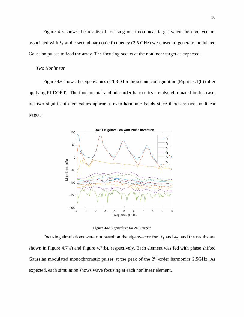
Figure 4.6 shows the eigenvalues of TRO for the second configuration (Figure 4.1(b)) after

applying PI-DORT. The fundamental and odd-order harmonics are also eliminated in this case,

but two significant eigenvalues appear at even-harmonic bands since there are two nonlinear

targets.

Figure 4.6: Eigenvalues for 2NL targets

Focusing simulations were run based on the eigenvector for λ1 and λ2, and the results are

shown in Figure 4.7(a) and Figure 4.7(b), respectively. Each element was fed with phase shifted

Gaussian modulated monochromatic pulses at the peak of the 2nd-order harmonics 2.5GHz. As

expected, each simulation shows wave focusing at each nonlinear element.

19

Figure 4.7: Focusing for 2NL targets with (a) eigenvalue 1 and (b) eigenvalue 2

Discussion

The simulated results verify the proposed technique of combining DORT with pulse-

inversion to selectively focus energy to NL targets via harmonic detection. The cases demonstrate

the technique applied to two cases: the first configuration (one linear target and one nonlinear

target) and the second configuration (two nonlinear targets).

In the results of the case of one linear and one NL target, eigenvalue mixing is observed

where the eigenvector at the fundamental frequency (1.25 GHz) associated with λ1is observed to

focus towards the linear target, and at the second harmonic (2.5 GHz) it is observed that the first

eigenvalue focus to the NL target. One likely explanation of this is that in the singular value

decomposition of the Hermitian conjugate of the transfer matrix the singular values are placed in

descending order. At the fundamental frequency the linear target is the strongest scatterer, thus the

corresponding eigenvector and eigenvalue appear at the first eigenvalue. Whereas the second order

harmonic the only response is from the NL scatterer. This phenomeon will be addressed in the

future work.

20

5. DESCRIPTION OF MODEL

The section of this thesis serves to describe the individual components of the experimental

set up including the experimental procedure. This section is provided for readers who wish to learn

more detail about the development of the testbed. This section may be skipped and there would

still be continuity. However, for a more comprehensive description of the chronological testbed

development the reader is urged to continue.

Vivaldi Antenna

Conventional technology for broadcast and communications utilize narrowband signals to

transmit data. There is interest amongst researchers using ultra-wideband (UWB) signals for

communications, imaging, radar, etc. UWB offers advantages over electromagnetic compatibility

over other systems. The power spectrum is dispersed over a large range of frequencies such that

no piece of the spectrum penetrates above the noise floor. Because of this, UWB signals can coexist

with conventional narrowband broadcast signals without interfering with them and are also more

immune to interference from them.

A Vivaldi antenna is an exponentially tapered slot antenna which is often used for UWB

radar and imaging applications because of its broadband performance and good directionality. As

illustrated in Figure 5.1, an electric field develops a curvature as the wave transitions from the

antenna to free space, a bowing which limits the gain or directionality of the antenna. As an aside,

a related investigation on the use of spatially-variant electromagnetic materials to further improve

the Vivaldi’s directivity is reported in Appendix C of this thesis.

21

Figure 5.1: Electric Field lines on a Vivaldi antenna

The antenna designed for this experiment is an antipodal variation of the Vivaldi antenna

where two exponentially tapered conductor flares separated by a dielectric are fed with a microstrip

transmission line.

Figure 5.2: CST Model of Vivaldi Antenna

The radiating bandwidth of the antenna is commonly held as those frequencies where the

return loss is less than -10dB, shows a bandwidth which spans from 1.1GHz to 20 GHz as shown

in Figure 5.3.

22

Figure 5.3: Measured and Simulated Return Loss for two Vivaldi antennas

A useful figure of merit for the antenna is the usable gain bandwidth. We are interested in

the antenna’s radiation in the direction of the targets. It is desired that the antenna to have a realized

gain of greater than 10 dB in the direction of propagation over the operating frequency, which will

henceforth be known as the usable gain bandwidth. To measure this a pair of antennas were placed

in the far-field of each other, and the transmission was measured using a vector network analyzer

(VNA) as shown in Figure 5.4.

Figure 5.4: Usable Gain Bandwidth measurement setup

Using the Friis transmission equation (5.1) the realized gain, including reflection loss, is

extracted and compared to simulation.

23

𝑃𝑃𝑟𝑟𝑃𝑃𝑡𝑡

= 𝐺𝐺2 �𝜆𝜆

4𝜋𝜋𝜋𝜋�2

(5.1a)

𝐺𝐺 = �4𝜋𝜋𝜋𝜋𝜆𝜆��𝑆𝑆21, 𝑆𝑆21 =

𝑃𝑃𝑟𝑟𝑃𝑃𝑡𝑡

(5.1b)

The realized gain vs. frequency in Figure 5.5 shows a usable bandwidth spanning from 3

to 12 GHz.

Figure 5.5: Usable Gain Bandwidth for Vivaldi antennas

Antenna Array

Array spacing is a critical parameter which determines the sampling angle for spatial

sampling of the environment. A widely spaced array, or more commonly known as a distributed

antenna network, can have significant spatial sampling. However, the focusing of a distributed

antenna network tends to introduce grating lobes resulting in less focusing. As the array spacing

decreases, the angle of spatial resolution increases. Consider Figure 5.6; the point target is assumed

to be in the far-field for the array such that the Fraunhofer approximation can be applied.

24

Figure 5.6: Illustration of the Fraunhofer approximation in an array

Using the Fraunhofer approximation, one can infer the angle at which the target is located

off the normal of the broadside of the array is the same for each element in the array, and can be

approximated so that:

∆𝑙𝑙 = 𝑑𝑑 sin∆𝜑𝜑 (5.2)

The differential length ,∆𝑙𝑙 , is limited by the sampling rate of the receiver and can be

expressed as the following:

∆𝑙𝑙 = ∆𝑡𝑡 ∙ 𝑐𝑐 (5.3)

Where (∆𝑡𝑡) is the minimum time-step of the receiver and (𝑐𝑐) is the speed of propogation in

free space. By substituting (5.3) into (5.2) and solving for (∆𝜑𝜑):

∆𝑡𝑡 ∙ 𝑐𝑐 = 𝑑𝑑 sin∆𝜑𝜑 (5.4a)

∆𝜑𝜑 = sin−14∆𝑡𝑡 ∙ 𝑐𝑐𝑑𝑑

(5.4b)

25

Distributed Antenna Network

In a distributed antenna network the target is assumed to be in the far-field for each antenna

element but not for the entire array – DORT does not require the target to be in the far-field of the

array. A large antenna spacing reduces the effect of inter-element coupling which can make

measurements difficult by exceeding the dynamic range of the receiver since the signals given by

inter-element coupling can have a magnitude much larger than the expected response from a target.

Another advantage to a distributed antenna network is that there is a greater spatial

resolution because the path length between elements is greater in a distributed network than a tight

array.

Linear Target

The first DORT measurements were taken with linear targets to simplify measurements as

the testbed was developed and refined. Measurements from the multi-static array were taken with

a metallic sphere placed in the center of the array cross-range and at 1.5 meters in down-range

shown in Figure 5.7.

Figure 5.7: Metal sphere suspended in interrogation environment

26

The sphere was modeled in CST Microwave Studio® (CST MWS) with a plane wave

excitation to determine its scattering pattern in Figure 5.8.

Figure 5.8: Simulated RCS pattern of a PEC sphere

Nonlinear Target

As shown in Figure 5.9, Schottky diodes made by Broadcom (HSMS2860) are placed at

the feed points of broadband bowtie antennas to serve as NL targets. The bowtie antenna was

fabricated on 1.02 mm thick Rodgers substrate (RO4730) with a relative permittivity of 3.

Figure 5.9: Bowtie antenna for NL targets

27

An important parameter to look at is the scattered signal (at 3 GHz) and radiation (at 6 GHz) pattern

shown in Figure 5.10 given by a plane wave excitation. This is important because RCS is directly

related to the power received by the diode which needs to be large enough to generate harmonics.

Figure 5.10: Bowtie Antenna for NL Targets (a) Scattering Pattern at 3 GHz and (b) radiation pattern at 6 GHz

Interrogation Pulse

The pulsed used in simulation and experimentation is a sinusoidal modulated Gaussian

pulse with a bandwidth of 2 GHz centered at 3 GHz. The time domain and frequency domain

representation of the pulse is shown in Figure 5.11.

Figure 5.11: Interrogation Pulse

(a) (b)

28

DORT Processing Script

To process the experimental data, the DORT time-domain multi-static dataset which

includes the mono-static and bi-static responses, is input into the DORT Matlab script (provided

in Appendix B). The code first extracts the time-domain data from each measurement and places

it into a matrix with rows equal to the number of time samples and columns equal to the number

of elements in the array squared. For example, an experimental set up with a four-element array

will appear as the following.

Figure 5.12: Data Import matrix in the time-domain

The matrix shown in Figure 5.12 is broken up into 4 sections where each section represents

a column in the multi-static matrix, that is that each section is broken up by the data sets provided

by the transmit antenna. In the figure above the blue section contains all the data where antenna 1

is the transmit antenna, the green section where antenna two is the transmit antenna, the beige

section where antenna 3 is the transmit antenna, and finally orange section where antenna four is

the transmit antenna. The matrix is then transferred to the frequency domain by means of Fourier

transform Figure 5.13.

Figure 5.13: Data-Import matrix in the frequency domain

29

This data can be portrayed in three dimensions and arranged in four frames where each

frame is mapped to one of the sections shown in the matrix above.

Figure 5.14: multi-static matrix unarranged

Notice the coordinates of the matrix above (Figure 5.14), the matrix has the coordinates

𝑡𝑡 × 𝑗𝑗 × 𝑖𝑖 and DORT works with the matrix 𝑖𝑖 × 𝑗𝑗 × 𝑡𝑡. A simple permute function in Matlab allows

us to change the order of the dimensions of any matrix so the data can be rearrange like the

following (Figure 5.15 same figure as Figure 3.2) which is the matrix that can be used for DORT

processing.

Figure 5.15: Multi-static data matrix in time domain

30

Experimental Procedure

The workflow for completing the DORT signal processing is shown in Figure 5.16. The

workflow can be broken up into three distinct stages – interrogation, identification and

transmission.

Figure 5.16: Workflow diagram for DORT experiment

The environment is illuminated with a short UWB pulse from an antenna array. Time

domain data is extracted from simulation or oscilloscope. The data is then processed in Matlab,

where the data is arranged into a multi-static 𝑁𝑁 × 𝑁𝑁 matrix (𝑁𝑁 is the number of array elements)

and transformed into the frequency domain. Then we employ the time-reversal operator (TRO)

and take the single-value decomposition (SVD) of the matrix. The entire band of eigenvalues and

eigenvectors are used to generate TR pulses for UWB focusing to overcome multipath and

complex environments. A more simplistic approach is using a monochromatic signals when there

is line-of-sight of the target to the array a set of phase shifted sinusoidal waveforms are generated

with the phase of the eigenvectors associated with the frequency. The sinusoidal waveform is then

31

truncated with a Gaussian window. In simulation the waveforms are Gaussian-windowed

monochromatic signals.

The Testbed for the validation of DORT combined with PI is broken up into three parts,

the computer (signal processing), the instrumentation, and the environment. Signal processing is

exclusively performed using Matlab (see Appendix B). The instrumentation utilizes the available

benchtop equipment including a 12.5 GHz dual-channel arbitrary waveform generator

(AWG70002A), a 2-20 GHz power amplifier (RM20220), and a 12.5 GHz high-speed oscilloscope

(MSO71254C).

Figure 5.17: Benchtop Instrumentation for Experiment

The first step in DORT is the interrogation of the environment using a short pulse

distinguishable in time. A pulse generated from Matlab (see Appendix A) is fed into the Tektronix

AWG. The AWG has two channels 1 and 2 with two differential ports as shown in Figure 5.17.

Channel 1 is amplified by the broadband amplifier which is then fed to the radiating antenna input.

Amp Scope

AWG

32

Channel 2 will emit another pulse, delayed by 30ns to trigger the oscilloscope so that it can collect

the scattered pulse return.

The output of channel 1 on the AWG feeds the input to an RF amplifier which provides

40dB of gain. The amplified pulse is then transmitted by a Vivaldi antenna. It is important that the

Vivaldi antenna is facing the target in this experiment. This experiment power constrained which

creates difficulty in exciting the nonlinearities of the diode. Therefore, to overcome path loss, the

antennas need to have a high directivity to deliver maximum power to the diode.

The first case considered in this experiment was using a metallic sphere, similar to that of

an RCS calibration sphere, to represent a linear target. Originally our antenna array spacing was

5 𝑐𝑐𝑚𝑚 which was at the maximum spacing of 𝜆𝜆2 where 𝜆𝜆 = 10 𝑐𝑐𝑚𝑚 before grating lobes would be

seen in focusing. Grating lobes are when maxima occur where it is unexpected because the spacing

of the array are greater than 𝜆𝜆2 such that maxima are repeated at unintended degrees of theta. This

can be demonstrated via simulation. Consider an array of 𝜆𝜆2-length dipole antnnas. The target

frequency is 3 GHz and 𝜆𝜆 = 10 𝑐𝑐𝑚𝑚. In Figure 5.18(a) the spacing is 10 cm and in Figure 5.18(b)

the spacing is 5 cm.

Figure 5.18: Demonstration of grating lobes with spacing (a) at 10 cm and (b) at 5 cm

33

The spacing 10 cm creates significant grating lobes at angles at theta equal to + −⁄ 90

degrees, whereas no grating lobes exist with a spacing of 5 cm.

Figure 5.19 shows the initial test set-up. The sphere was placed 1.5 meters in down-range

from the array with an element-spacing of 5cm with 6 elements. The array measurements were

taken in a series of discrete measurements involving two antennas at a time by fixing the transmit

antenna and changing the position of the receive antenna. After the first column of the multi-static

matrix is filled, i.e., the receive antenna has been moved to each position, the position of the

transmit antenna is changed, so the measurements for the next column of the multi-static matrix is

acquired. This process is repeated for each column in the multi-static matrix. The sphere is then

removed, and the measurements are repeated to obtain a background which will be used later to

de-embed effects of inter-element coupling.

Figure 5.19: Initial Experimental Setup

Next, the signals are processed using the DORT code (Appendix B) which was verified by

simulation. The initial results are shown below in Figure 5.20.

34

Figure 5.20: Initial DORT results: one linear target

There are several things in this figure that are not desirable. First, there is no significant

separation of eigenvalues. Since there is only one target in the field, there should only be one non-

zero eigenvalue ideally. Next, it is seen that there are harmonics at every integer multiple of 2.5

GHz which, for this case, was the center frequency of the transmit pulse. And there is also an

unexpected signal at 500 MHz.

The first thing investigated was the separation issue. At this time the harmonics generated

were not the primary concern since this could be explained by nonlinearities in the oscilloscope or

amplifier. It was determined that the antenna coupling was affecting our ability to resolve the

target, that a relatively large amount of energy was being coupled directly between antenna

elements, creating difficulties in correctly processing the smaller signals from the target. Looking

at some time-domain data shown in Figure 5.21.

35

Figure 5.21: Initial bi-static result one linear target (a) raw measurement (b) background subtracted

In Figure 5.21(a) the raw measurement for a single bi-static measurement (m16) is plotted.

One trace is with the sphere, and one is without the sphere. While it is visible, one can see there is

little difference in the two traces. At around 45ns the trace with the sphere (blue) peaks out from

behind the background measurement (orange). Next, we subtract the background from the trace

with the sphere, and the resulting plot is shown in Figure 5.21(b) even though the background is

subtracted out there is some quantization noise that is so great that the subtracted “error” is greater

than the signal we are trying to see. The antenna coupling (circled in red) is thought to be the pulse

circled in red because the difference in time that the two pulses arrive (green minus red) is around

10ns which is the expected time of arrival. For a 3 meter (1.5 * 2) path length at 3 × 108 m s⁄ for

propagation velocity, the time expected time of arrival is 10 ns. So it can be inferred that the pulse

circled in red represents the inter-element coupling subtraction error and the pulse circled in green

represents the scattered response from the metal sphere. Another difficulty encountered was that

it appeared that the pulses received by each bi-static measurement were arriving at the same time

because the time difference was smaller than the oscilloscope sampling rate as explained below.

When considering the path length difference we had the following shown in Figure 5.22.

36

Figure 5.22: Relative path length differences

The relative path length difference between the green path and the blue path can be

calculated as follows:

∆𝑙𝑙 = �0.0252 + 1.52 − �0.0752 + 1.52

∆𝑙𝑙 = 1.7 × 10−3𝑚𝑚

Relating the relative path difference to time we get:

𝑡𝑡 =∆𝑙𝑙𝑐𝑐

𝑡𝑡 = (1.7 × 10−3)/(3 × 10−8)

𝑡𝑡 = 5.5 𝑝𝑝𝑝𝑝

37

The expected time between each pulse is 5.5 ps which is much less than the sampling rate

of the scope (20 ps/sample). Therefore the oscilloscope could not possibly distinguish the arrival

time for each path. This same limitation was also the possible source of the difficulty in separating

the eigenvalues.

To address this challenge, the antenna array was spaced out which gives a larger path length

difference that can be resolved by the oscilloscope as well as having the added benefit of reducing

inter-element coupling. The new test set up is shown below in Figure 5.23.

Figure 5.23: Second Experimental Setup (a) Functional Diagram (b) Anechoic Chamber Photo

38

The array size was reduced to four elements, and there were four antennas fabricated to be

stationary in the chamber to improve repeatability between measurements. The cables for each of

the antennas (𝐿𝐿1, 𝐿𝐿2, 𝐿𝐿3, 𝐿𝐿4) are all close to equal in length to keep consistent phase progression

from the antenna to the scope. A splitter is used for the mono-static measurements. The signal

from the amplifier passes through port 1 of the splitter/combiner and leaves through the common

port remaining isolated from the scope by 20 dB, so that that the signal does not exceed the port

input power limits of the scope. The scattered response comes back through the common and half

the power goes to the scope and the other half gets “reflected” back to the amp. That power is so

small however that there is no risk of harming the amplifier. With the new set up we obtained the

results shown in Figure 5.24.

Figure 5.24: Second Experimental results

It is clear that some harmonics remain along with a 500 MHz signal; however what is most

concerning is still no significant separation between eigenvalue. Up to this point, we have been

looking at the eigenvalues on a dB scale. If you look at the eigenvalues on a linear scale, it is clear

that we are close to resolving the target (see Figure 5.25)

39

Figure 5.25: Second Experimental results linear scaling

Looking at the time domain data we can make more sense about the observation (see Figure

5.26).

Figure 5.26: Initial bi-static result one linear target (a) raw measurement (b) background subtracted

Similar to before we can see the response of the sphere emerging from beneath the

background measurement. After background subtraction, the resulting curve is plotted in Figure

5.26(b), and it is clear that the target response is greater than the other noise. To try to clean up the

40

data time gating was used as a means of ignoring the other artifacts in the measurement and

isolating the target response only. The following eigenvalues were acquired (see Figure 5.27).

Figure 5.27: Second Experimental results linear scaling after time-gating

It appears that time-gating does a great job in cleaning up the signal and also grants

significant separation between eigenvalues. It appears that a single linear target has been resolved.

While resolving the linear target was a major milestone there is still work to be done. After

all, the purpose of this thesis is to detect and selectively focus waves at NL targets by identifying

them by their harmonics. In the following experiment, the metal sphere was replaced with a bowtie

antenna with rounded corners, but the distance to the target (down-range) was changed from 1.5

m to 60 cm see Figure 5.28.

41

Figure 5.28: NL Experimental setup

Without employing the entire DORT method we sought to extract NL harmonics in a

simple bi-static case. We were unsuccessful in turning the diode on to generate harmonics. At this

point, the design of the target antenna was altered so a greater voltage was made available to the

diode so that it might turn on. With the new antenna design, the harmonics can be distinguished as

shown in Figure 5.29

Figure 5.29: NL Bi-static test (a) time domain and (b) frequency domain

42

The plots shown in Figure 5.29 show the data resulting from pulse inversion. A few things

to note are that there is definitely a harmonic generated at 6 GHz but also significant ringing at

500 MHz which is also visible in the time-domain. It was then determined that the 500 MHz

ringing was coming from the amplifier. To clean up the signal a mini-circuits high-pass filter

(passband f>2GHz) was placed on the input of the scope, and the 500 MHz ringing was resolved.

Full DORT was then performed on the single diode. The results are shown in Figure 5.30

Figure 5.30: Nonlinear Experimental results in linear scaling

The eigenvalues indicate that the diode is being turned on and harmonics are generated.

The 500MHz signal is eliminated; however, there seems to be some difficulty in separating the

eigenvalues once again. It is again useful to look at what is going on in the time-domain.

43

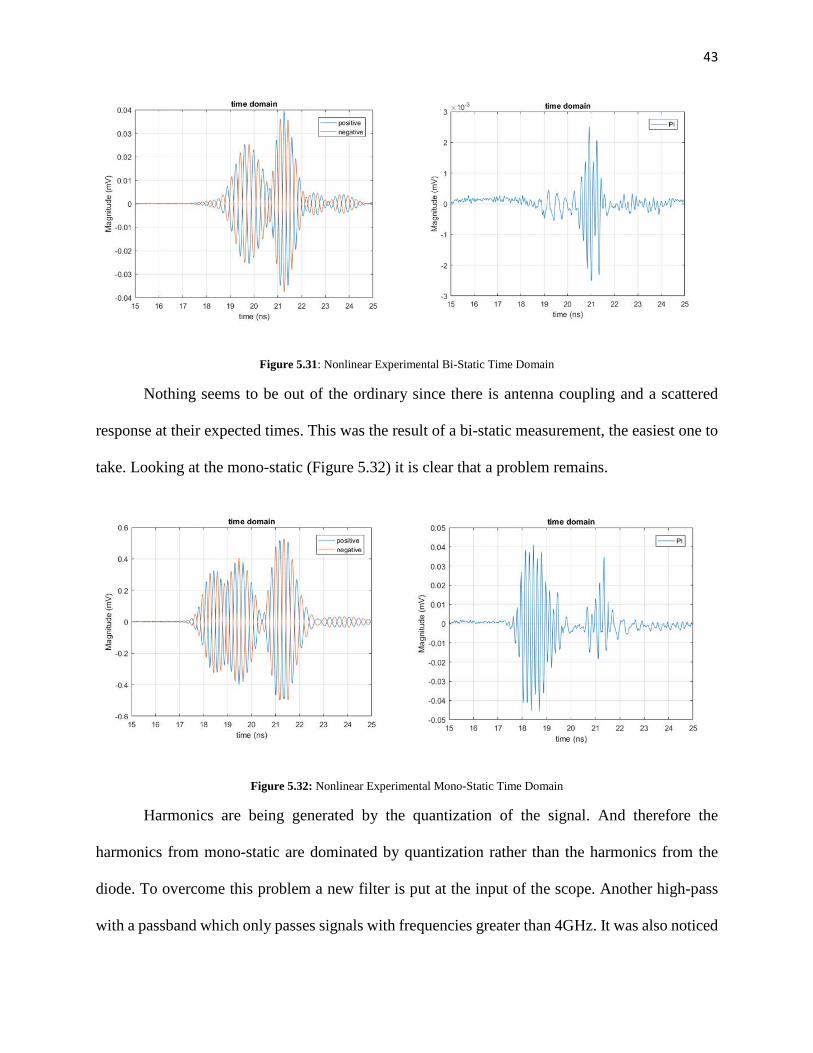
Figure 5.31: Nonlinear Experimental Bi-Static Time Domain

Nothing seems to be out of the ordinary since there is antenna coupling and a scattered

response at their expected times. This was the result of a bi-static measurement, the easiest one to

take. Looking at the mono-static (Figure 5.32) it is clear that a problem remains.

Figure 5.32: Nonlinear Experimental Mono-Static Time Domain

Harmonics are being generated by the quantization of the signal. And therefore the

harmonics from mono-static are dominated by quantization rather than the harmonics from the

diode. To overcome this problem a new filter is put at the input of the scope. Another high-pass

with a passband which only passes signals with frequencies greater than 4GHz. It was also noticed

44

that there were some harmonics coming out of the amplifier. So a band-pass was placed on the

output of the amplifier, and the pulse was redefined to fit the band of the filter (center frequency

= 2.9 GHz with a bandwidth of 400 MHz). See Figure 5.33 for new test setup

Figure 5.33: NL Experiment Setup

It is desirable that the system inside the blue area is completely linear, with the exception

of the target, so the band-pass filter (Mini-circuit VBF-2900+) and the high-pass filter (Mini-

circuit VHF-4600+) are used to ensure that the only harmonics that will reach the scope are

physical from the diode. With the new set up we acquired the results shown below.

Figure 5.34: Nonlinear Experimental results in linear scaling

45

At this point, the results indicated that the experimental testbed was nearing completion if

the eigenvalues could be separated to a greater extent. It was determined at this point that the power

being reflected from the antenna in the mono-static measurements were greater than the signal

received. This is due to the slight impedance mismatch of the Vivaldi antenna with the 50 W

transmission line. To solve this problem, a quasi-mono-static set up was developed whereby the

measurements are taken in the same procedure as bi-static which two antennas on either side of

the transmit antenna and take a geometric mean of the frequency domain response of the mono-

static measurement this gives us the same magnitude (assuming the magnitude doesn’t change

from one antenna to the other) and average phase to give the expected phase at the true mono-

static point (see Figure 5.35). This procedure is called a quasi-mono-static measurement.

Figure 5.35: Quasi-mono-static measurement

The resulting eigenvalues from this new technique are shown in Figure 5.36

46

Figure 5.36: Nonlinear Experimental results in linear scaling

There appears to be great separation between eigenvalues for these NL targets; however

the phase of the eigenvectors do not appear to indicate the direction of the target. It is assumed that

the relative phase for each element of the eigenvector associated with the nonzero eigenvalue

relates the position of the target relative to each other element. For an antenna array, this indicates

the direction of the target in the environment. This assumption is only true if the given elements

in the array are consistent in terms of phase progression. Slight fabrication variations in the

antennas and cables can make the phases unpredictable meaning that they have no bearing on

where the object is in the environment. For the experiment, it is desirable that the only source for

a relative phase difference between elements is the relative path length differences from the

transmit antenna to the target and back to the different elements in the array.

47

6. EXPERIMENTAL PI-DORT

This section serves to provide the results of combining DORT with PI to detect, locate, and

focus on nonlinear elements in numerical simulation and measurement. The cases investigated for

both simulation and measurement include the following:

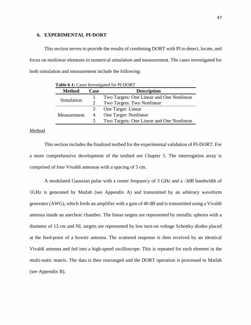
Table 6-1: Cases Investigated for PI-DORT Method Case Description

Simulation 1 Two Targets: One Linear and One Nonlinear 2 Two Targets: Two Nonlinear

Measurement 3 One Target: Linear 4 One Target: Nonlinear 5 Two Targets: One Linear and One Nonlinear

Method

This section includes the finalized testbed for the experimental validation of PI-DORT. For

a more comprehensive development of the testbed see Chapter 5. The interrogation array is

comprised of four Vivaldi antennas with a spacing of 5 cm.

A modulated Gaussian pulse with a center frequency of 3 GHz and a -3dB bandwidth of

1GHz is generated by Matlab (see Appendix A) and transmitted by an arbitrary waveform

generator (AWG), which feeds an amplifier with a gain of 40 dB and is transmitted using a Vivaldi

antenna inside an anechoic chamber. The linear targets are represented by metallic spheres with a

diameter of 13 cm and NL targets are represented by low turn-on voltage Schottky diodes placed

at the feed-point of a bowtie antenna. The scattered response is then received by an identical

Vivaldi antenna and fed into a high-speed oscilloscope. This is repeated for each element in the

multi-static matrix. The data is then rearranged and the DORT operation is processed in Matlab

(see Appendix B).

48

Results

The results for the following cases are presented here: one linear target, one NL target, one

linear and one NL targets. The results also investigate using a distributed element system and a

beam form array. A distributed element system is when the spacing between antennas is further

than what would be considered a tightly spaced beam-forming array, and can be useful for

sampling the field with greater resolution.

One Linear Target

The eigenvalues generated from DORT (see Appendix A) from one target show a clearly

dominant eigenvalue (λ1) as shown in Figure 6.1 and the phase of the eigenvectors demonstrate

that the target was placed closest to the third element in the array. The smaller non-zero

eigenvalues (λ2-λ4) may be explained by other modes introduced by the sphere since the scattering

is no longer a point scatterer.

Figure 6.1: Eigenvalues and eigenvectors from one linear target.

49

Significant separation of the eigenvalues at 3 GHz implies one linear scatterer detected.

Based on the phase of the eigenvector at 3GHz it can be seen that the target is closest to elements

2 and 3 of the array indicating that the target is located in the center of the field.

One Nonlinear Target

The eigenvalues generated from DORT (see Appendix A) from one target show a clearly

dominant eigenvalue (λ1) as shown in Figure 6.2 and the phase of the eigenvectors demonstrate

that the target was placed closest to the third element in the array. The smaller non-zero

eigenvalues (λ2-λ4) may be explained by other modes introduced by the bowtie antenna since the

scattering is no longer a point scatterer.

Figure 6.2: Eigenvalues and eigenvectors from one linear target.

Significant separation of the eigenvalues at 5.8 GHz implies one nonlinear scatterer

detected. Based on the phase of the eigenvector at 5.8 GHz it can be seen that the target is closest

to elements 2 and 3 of the array indicating that the target is located in the center of the field.

50

Another set of measurements were taken by using an array rather than a distributed antenna

network. This is so that the beam-width of each Vivaldi antenna could cover the interrogation field.

For a spacing of 5cm and using the quasi-mono-static technique described in section 5 the results

for an off-centered to the left diode are shown in Figure 6.3

Figure 6.3: Eigenvalue and Eigenvector for off-centered diode using a closely spaced array

The results shown in Figure 6.3 show significant separation between eigenvalues at the

harmonic band of 5.8 GHz. Again an explanation of why there are multiple nonzero eigenvalues

is that multiple modes may be received by the array seeing that the target is extended and may not

be fully resolved. At the fundamental band (2.9 GHz) there is significant suppression of the

fundamental however there is no complete canceling. That being said the fundamental is

suppressed enough so that the harmonic band can be discerned. The eigenvectors indicate that the

target is located towards the left side of the array.

51

One Linear and One Nonlinear Target

Another case that was investigated was using PI-DORT with the presence of one linear

target and one NL target. Using an array spacing of 5 cm, with the targets placed 1.2 m away both

off center. The linear target is represented by a bowtie antenna identical to the one used for the

nonlinear target. However, there is no diode soldered across the feed point. The set up can be seen

in Figure 6.4

Figure 6.4: One linear and One NL experimental setup, diode is on the left and linear target is on the right

In the experimental setup, the targets were placed 1.2 m down range and the NL target

resides on the left side of the array and the linear target resides on the right side of the array. Pulse

inversion mitigates the effect of linear targets therefore it doesn’t make sense to use pulse inversion

if the location of the linear target is desired. This is why the results shown in Figure 6.5 use

background subtraction.

52

Figure 6.5: One Linear and One Nonlinear Target using Background subtraction eigenvalues

Even though the detection and location of linear targets is not important to the work reported in

this thesis, these results show why combining PI and DORT is so useful. Without prior knowledge

of the linear and NL target, it would be impossible to discern the two. The harmonics are also

difficult to see in comparison to the fundamental response. PI-DORT is shown in Figure 6.6

Figure 6.6: One Linear and One Nonlinear Target using PI-DORT

53

The fundamental frequency component is greatly reduced and the harmonics are much

more visible when PI-DORT is employed. The eigenvector also shows that the nonlinear target is

on the left side of the array just as the targets are set up.

Discussion

The measurements show a successful identification of NL targets. However, there are

considerable components showing up in the secondary eigenvalues even when there is only one

target in the environment. As discussed before the targets have an extent to them which may excite

multiple modes that may appear as multiple targets.

Another cause may be the chamber itself. The chamber was designed to be anechoic at

above 7 GHz and lower than that the chamber may be more reverberant. So rather than the modes

being caused by an extended target the multiple-modes could be chamber modes that are excited.

The root cause is difficult to know for sure.

In summary, the experiment was successful in its goal, to demonstrate PI-DORT in a 3D

physical experiment. There are discernable eigenvalues with corresponding eigenvectors that have

some indication of the whereabouts of the targets. The value in using PI-DORT over traditional

DORT is that the harmonics from nonlinear targets become much more visible compared to the

fundamental frequency, which opens the door to a variety of applications.

54

7. FUTURE WORK

There are several avenues for future work in PI-DORT. The work reported here provides

a foundation upon which to build future investigations. Some of the limitations previously

discussed can be resolved by improving the antenna design for both the target and interrogator.

Also creating frequency dependent targets could greatly increase the capability of DORT and open

the technique up to a variety of applications.

Addressing the Eigenvalue mixing problem

As previously reported, there are instances where targets with a different frequency

response, such as linear and non-linear targets, the eigenvalue can be mixed if the most dominate

scatter at one frequency is different as the most dominate scatterer at another frequency. For

example, linear targets tend to scatterer a stronger fundamental than a nonlinear target. Therefore,

as seen with the simulated PI-DORT results, there is a mixing of eigenvalues and eigenvectors as

a function of frequency.

An algorithm can be employed which exploits a property of the eigenvectors that the

eigenvectors, 𝑽𝑽(𝜔𝜔𝑜𝑜), at a given frequency are orthogonal from one another. The eigenvectors can

be seen to be orthogonal from each-other when the inner product of the two eigenvectors are

identically zero, i.e.

⟨𝑽𝑽𝑖𝑖(𝜔𝜔𝑜𝑜),𝑽𝑽𝑗𝑗(𝜔𝜔𝑜𝑜)⟩ = 0 (7.1)

In most mediums, the greens function should not experience abrupt changes in its frequency

response. Therefore, the eigenstructure can be rearranged such that the adjacent frequency points

of the eigenvector are correlated [9].

55

Furthering performance with Improved Antenna Design

Applications which can employ DORT can be practically improved with improvements on

the interrogator array, and more specifically the individual antenna elements of the array. With

improved directivity of an array element, the resolution of the image can be greatly improved.

Attached in Appendix C is a paper describing how the gain Vivaldi antennas used could be

improved by employing a spatially variant and anisotropic dielectric lens in front of the radiator.

The target antenna could also be adapted to have a wider backscattered beam-width so that

the backscattered signal can be seen by a wider array. Currently, there is a lot of energy wasted

because the target antenna reradiates in two directions: one direction facing the array and the other

direction facing away from the array. Designing an antenna with a larger backscatter may enable

the investigation of more cases where the antenna orientation and location is less important.

Frequency Signatures

For many applications, it is desirable to know more about the target than whether or not it

is linear or nonlinear. For the experiment carried out in this thesis the targets were largely

frequency independent in their scattering characteristics. However, it is often the case that targets

of interest will have frequency characteristics. For example, a cell phone typically operates in a

frequency band of 2.4 GHz while a drone may communicate at 5.8 GHz and therefore a drone and

a cell phone could have drastically different frequency responses. Future work could include

frequency-dependent targets where there exists a certain frequency characteristic to give the target

a frequency signature to further identify the type of target that is in the environment.

A way to demonstrate this is to change the antenna design from a wide-band bow-tie

antenna to a more resonant dipole antenna. A demonstration can include two targets with slightly

56

different length dipoles such that they can be distinguished while falling within the band of the

interrogation pulse, or target antennas with DC-biased varactor diodes so the harmonic response

is tunable.

Potential Applications

Once the limitations have been addressed, there are several applications that can be

investigated. PI-DORT provides an answer to many difficult problems in imaging, radar, and

communications. The experimental setup described in this thesis can be altered to better suit many

applications which may include biomedical imaging, wireless power transfer, security and defense,

and cellular communications. Chapter 8 of this thesis provides a survey of potential applications

which can be investigated.

57

8. Survey of Applications

The detection and selective focusing at nonlinear targets have many applications including

biomedical imaging, wireless power transfer, security and defense, and cellular communications.

This section of the thesis provides a short survey of the possible areas of application in which PI-

DORT can be utilized.

Biomedical Imaging and Microwave Thermotherapy

An application of DORT is in medical imaging. Originally DORT was utilized in

ultrasound imaging of kidney stones. In order to illustrate the potential for electromagnetic

imaging, consider a breast cancer tumor. If NL nanoparticle were incorporated into the tumor, PI

DORT would be used to detect the presence of a tumor [9]. If the nano-particles in question were

metallic, it might prove feasible via focused radiation to heat and perhaps eliminate the tumor,

with much less damage to the surrounding tissue.

Wireless Power Transfer

Another application for DORT is wireless power transfer. With the rise of IoT, one hurdle

is to be able to power a wireless sensor network. Broadcast towers radiate information in an

omnidirectional pattern; however the device that needs the information is located at some point in

the “area” that the broadcast antenna can cover; therefore, there is RF energy that is unused

everywhere. There is currently a large interest in RF energy harvesting similar to solar-panels, but

for lower frequencies, and with the rapid growth of low energy devices emerging on the market,

the ambient energy may be enough to supply these devices.

58

Rectennas have nonlinear attributes to them which can be detected and DORT is a way to

efficiently harvest energy for a low energy device. DORT can be a way of achieving this by

selectively charging sensors without the need for human intervention

Security and Defense

DORT may be of interest for defense applications. With the rise of drones in the consumer

market, it may be difficult to detect an unmanned aerial vehicle in a secure airspace. Drones within

the airspace can be identified and tracked, and also if necessary a jamming signal can be sent to

the drone to remove it from the airspace.

IEDs are usually triggered by cell phones. By employing PI-DORT, these cell phones can

be identified as a threat or not. If the threat is deemed necessary to intervene direct high powered

microwaves can be transmitted to overload the target without damaging non-threatening

electronics which may be near-by.

5G Communications and IoT

There is a lot of interest in using TR for IoT and 5G communications. The reason being is

TR can effectively propagate a signal from the source to the destination regardless of the

environment. In fact, TR takes advantage of multipath to direct energy without the use of a massive

MIMO array.

59

9. CONCLUSION

This thesis set out to demonstrate the detection and location of nonlinear scatterers using

DORT combined with pulse inversion. Nonlinear scatterers are identified by harmonics occurring

at integer multiples of the fundamental frequency of the transmit pulse. Due to the law of

conservation of energy, a scattered response of the target is minuscule compared to the power

transmitted by the source. Therefore the magnitude of the harmonic is also tremendously small

therefore the receiver must be tuned to be sensitive enough to discern such a small scatterer.

However, there exist linear scatterers in the system that exhibit large responses compared to the

nonlinear scatterer. The response of the linear scatter can force the receiver outside its dynamic

range, which is the range defined to be linear, and excite harmonics that interfere with the response

from the nonlinear target of interest.

Pulse inversion is a technique used to cancel out the fundamental response of all targets,

which allows for the receiver to discern the nonlinear scatters in an environment with linear clutter.

Pulse inversion also eliminates the need to perform a background subtraction on the array. Antenna

coupling is a large obstacle in performing DORT. The technique cannot resolve a single target and

generates eigenvalues that are difficult to understand. Background subtraction is a technique which

can resolve this by taking the multi-static response with the target data and subtracting the multi-

static response with an empty environment (i.e., no targets) so that the antenna coupling is

subtracted out of the multi-static matrix. However, this is in many cases impractical since the

environments are typically dynamic and therefore performing a background subtraction on the

array may not work. With pulse inversion performing a background subtraction is not necessary

since the coupling between antennas is linear.

60

REFERENCES

[1] M. Fink, "Time reversed acoustics," Phys. Today, vol. 3, no. 50, pp. 34-40, 2004.

[2] C. Prada, S. Manneville, D. SPoliansky and M. Fink, "Decomposition of the Time Reversal Opperator: Detection and Selective Focusing on Two Scatterers," J. Acoust. Soc. Am, vol. 4, no. 99, pp. 2067-2076, 1996.

[3] G. Leosy, J. d. Rosney, A. Tourin, A. Derode, G. Montaldo and M. Fink, "Time Reversal of Electromagnetic Waves," Phys. Rev. Lett., vol. 19, no. 92, 2004.

[4] J. Faia, K. McClintik, and S. Hong, "Application of DORT and Pulse Inversion to Detection and Selective Electromagnetic Focusing of on Nonlinear Elements," in URSI GASS, Montreal, 2017.

[5] E. Barbiery and M. Meo, "Time reversal DORT method applied to nonlinear elastic wave scattering," Wave Motion, vol. 7, no. 47, pp. 452-467, 2010.

[6] M. E. Yavuz and F. L. Teixeira, "Full Time-domain DORT for Ultrawideband Electromagnetic Fields in Dispersive, Random Inhomogenous Media," IEEE Trans. Ant. Prop, vol. 8, no. 54, pp. 2305-2315, 2006.

[7] T. G. Leighton, G. H. Chua, P. R. White, K. F. Tong, H. D. Giffiths and D. J. Daniels, "Radar Clutter Suppression and Target Discrimination Using Twin Inverted Pulses," Proc. R. Soc. A, no. 469, 2013.

[8] S. K. Hong and e. al., "Nonlinear Electromagnetic Time Reversal in an Open Semireverberant System," Phys. Rev. Applied, no. 2, 2014.

[9] C.-L. Hsieh, Y. Pu, R. Grange, and a. D. Psaltis, "Digital phase conjugation of second harmonic radiation emitted by nanoparticles in turbid media," Optics Express, vol. 18, no. 12, 2010.

[10] D. H. Simpson, C. T. Chin and P. N. Burns, "Pulse Inverson Doppler: A New Method for Detecting Nonlinear echoes from Microbubble Contrast Agents," vol. 2, no. 46, pp. 372-382, IEEE Trans. Ultrason. Ferroelect. Freq. Control.

[11] Y. Chen, F. Han, Y.-H. Yang, H. Ma, Y. Han, C. Jiang, H.-Q. Lai, D. Claffey, Z. Safar and K. J. R. Liu, "Time-Reversal Wireless Paradigm for Green Internet of Things: An Overview," Internet of Things Journal, vol. 1, no. 1, pp. 81-98, 2016.

[12] Y. Chen, B. Wang, Y. Han, H.-Q. Lai, Z. Safar and K. J. R. Liu, "Why Time Reversal for Future 5G Wireless?," IEEE Signal Processing Magazine, pp. 17-25, 2016.

61

[13] D. Hossain and A. S. Mohon, "Cancer Detection in Highly Dense Breasts Using Coherently Focused Time-Reversal Microwave Imaging," IEEE Transactions on Computational Imaging, vol. 3, no. 4, pp. 928-939, 2017.

[14] Y. Mehdi, A. Ebrahimzadeh, M. Dehmollaian and A. Madannejad, "A Time-Reversal Imaging System for Breast Screening; Theory and Initial Phantom Results," IEEE Transactions on Biomedical Engineering, vol. PP, no. 99, pp. 1-1, 2018.

[15] S. K. Hong, "Effect of Target Resonances on Ultrawideband-DORT," Journal of Electromagnetic Waves and Applications, vol. Under Review, 2018.

62

APPENDICES

63

APPENDIX A—Pulse Generation Script

%% Generate Wide Band Pulse %%%%%%%%%%%%%%% % % Author: Joseph Faia % Last Updated: 3/2/2018 % %%%%%%%%%%%%%%%%%%%%%%%%%%%%%%%%%%%%%%%%%%%% %% Pulse Specs fh = 4;%GHz fl = 2;%GHz fo = 1e9*(fh+fl)/2; BW = 1e9*(fh-fl)/2; %fo = 2.9e9; %Fundemental Frequency %BW = 2e9; %Bandwidth 3dB fbw = BW/fo;%Fractional Bandwidth fs=25e9; %sample frequency dt=1/fs; %delta time PRF=1000e3; T=1/PRF; Np = 25000; % Number of points %td = 45e-9; %time shift td = 0; %original PW=20e-9; %pulsewidth N=T/dt; t = (-N/4*dt-td):dt:(N/4*dt-td); tt=(0:dt:dt*N); ts = (-5e-9*dt):dt:(N*dt+5e-9*dt); %% Generate Pulse x = 1*gauspuls(t,fo,fbw); y = 1*gauspuls(t,fo,fbw); z = [x y]; z = z(1:length(tt)); plot(tt,z); figure(2) plot(tt,z) Y = fft(x); f = linspace(0,1/dt,length(t)); figure(3) subplot(2,1,1) plot(t*1e9-527,x); xlim([0 12]); title('Time Domain and Frequency Domain Interrogation Pulse'); xlabel('Time (ns)'); ylabel('Normalized Magnitude'); subplot(2,1,2) plot(f*1e-9,abs(Y)/max(abs(Y))); xlim([0 12]); %ylim([-20 0])

64

xlabel('Frequency (GHz)'); ylabel('Normalized Magnitude'); %% Save to .mat file for AWG xx = [z(:,1:(length(tt)-1))';z(:,1:(length(tt)-1))']; Waveform_Name = 'CF_3GHz_BW_1GHz_pos'; Waveform_Data = xx(1:Np); save( [Waveform_Name '.mat'],'Waveform_Data','Waveform_Name','-v7.3');

65

APPENDIX B –PI -DORT Processing Script

%% Generate Wide Band Pulse %%%%%%%%%%%%%%% % % Author: Joseph Faia % Last Updated: 3/2/2018 % %%%%%%%%%%%%%%%%%%%%%%%%%%%%%%%%%%%%%%%%%%%% clear all clear clc close all N = 4; folder = 'C:\Users\faiajm\Documents\RHIT\2016-17\DORT\Summer2017_Thesis\Experimental Results\DORT\Data\3_28_18\diodeL\bi-static\'; folder2 = 'C:\Users\faiajm\Documents\RHIT\2016-17\DORT\Summer2017_Thesis\Experimental Results\DORT\Data\3_28_18\diodeL\mono-static\'; folder3 = 'C:\Users\faiajm\Documents\RHIT\2016-17\DORT\Summer2017_Thesis\Experimental Results\DORT\Data\2_2_17_1NL_2-4GHz\PathComp\'; Ns = 1000;%number of samples k = 1; sources = 4; %%%% Element Phase Error (rad) %%%%%% error_a1a = 0; error_a2a = 0.42; error_a3a = 0.76; error_a4a = 1.13; %%%%%%%%%%%%%%%%%%%%%%%%%%%%%%%%%%%%% [fs, S11s, S21s,~,~] = loadsNp([folder3 'splitter.s2p'], 9, 'MA', 0); %% IMPORT DATA for i = 1:N for j = 1:N if(i==j) P(:,k) = zeros(Ns,1); Nd(:,k) = zeros(Ns,1); Bp(:,k) = zeros(Ns,1); Bn(:,k) = zeros(Ns,1); X(:,k) = zeros(Ns,1); a(:,k) = zeros(Ns,1); myfilename_p = sprintf('p%d%da.txt',i,j); myfilename_n = sprintf('n%d%da.txt',i,j); myfilename_bp = sprintf('p%d%db.txt',i,j); myfilename_bn = sprintf('n%d%db.txt',i,j); filep = importdata([folder2, myfilename_p]); filen = importdata([folder2, myfilename_n]);

66

filebp = importdata([folder2, myfilename_bp]); filebn = importdata([folder2, myfilename_bn]); t = filep.data(:,1); tt = t*1e9; p_a = filep.data(:,2); p_b = filebp.data(:,2); p_a = p_a - mean(p_a); p_a = p_a - mean(p_b); Pma(:,k) = p_a; Pmb(:,k) = p_b; n_a = filen.data(:,2); n_b = filebn.data(:,2); n_a = n_a - mean(n_a); n_b = n_b - mean(n_b); Nma(:,k) = n_a; Nmb(:,k) = n_b; x_a = (p_a + n_a).*heaviside(tt-7).*heaviside(11-tt); x_b = (p_b + n_b).*heaviside(tt-7).*heaviside(11-tt); Xm_a = fft(x_a); Xm_b = fft(x_b); Xm_a = Xm_a; Xm_b = Xm_b; am_a(:,k) = Xm_a; am_b(:,k) = Xm_b; % k = k+1; else myfilename_p = sprintf('p%d%d.txt',i,j); myfilename_n = sprintf('n%d%d.txt',i,j); filep = importdata([folder, myfilename_p]); filen = importdata([folder, myfilename_n]); t = filep.data(:,1); tt = t*1e9; p = filep.data(:,2); p = p - mean(p); P(:,k) = p; n = filen.data(:,2); n = n - mean(n); Nd(:,k) = n; x = p+n; X(:,k) = x.*heaviside(tt-7).*heaviside(11-tt); eval(['a_temp = fft(x)*exp(sqrt(-1)*( error_a' num2str(j) ' + error_a' num2str(i) '));']); a(:,k) = a_temp; k = k+1; end end end %%%%Plot TD data%%%%%% figure(1) %plot(tt,P(:,2:4)*1e3,tt,Nd(:,2:5)*1e3); plot(tt,X(:,2:4)*1e3); %xlim([0 80]); xlabel('time (ns)'); ylabel('Voltage (mV)');

67

title('Bi-static Measurements after PI'); legend('h21', 'h31', 'h41'); figure(2) %plot(tt,Xma(:,1),tt,Xmb(:,1)); %xlim([0 80]); xlabel('time (ns)'); ylabel('Voltage (mV)'); title('Bi-static TD after Background Subtraction'); legend('h11a','h11b'); %%%%%%%%%%%%%%%%%%%%%%% %% DORT %%%%%% convert to Freq Domain %%%%%%% f = linspace(0,1/mean(diff(t)),length(P(:,1))); %%%%%%%%%%%%%%%%%%% Geometric Mean for Mono-static Data%%%%%%%%%%%%%% for jj=1:N^2 %am_abs(:,jj) = 1/2*(abs(am_a(:,jj))+abs(am_b(:,jj))); am_abs(:,jj) = sqrt(abs(am_a(:,jj)).*abs(am_b(:,jj))); am_phase(:,jj) = 1/2*(unwrap(angle(am_a(:,jj)))+unwrap(angle(am_b(:,jj)))); am(:,jj) = am_abs(:,jj).*exp(sqrt(-1)*am_phase(:,jj)); Xm(:,jj) = ifft(am(:,jj),'symmetric'); %am(:,jj) = sqrt(am_a(:,jj).*am_b(:,jj)); end %%%%%%%%%%%%%%%%%%%%%%%%%%%%%%%%%%%%% a = a + am; %Combine Mono-static and Bi-static Measurements for jj=1:N^2 a(:,jj) = heaviside(f-.5e9)'.*a(:,jj); % Filter end %%%%Rearrange Data Matrix%%%%%% for k=1:sources for j=1:sources M(:,j,k)= a(:,(k-1)*N+j); end end % t=A(:,1); M = permute(M, [2 3 1]); %%%%%%%%%%%%%%%%%%%%%%%%%%%%%%% %Frequency domain plot figure(3) plot(f*1e-9,abs(a(:,1:4)));xlim([0.1 10]); xlabel('Frequency (GHz)'); ylabel('Relative Magnitude'); title('first column freq. domain'); legend('M11','M21','M31','M41') %%%%%%%%%Apply DORT%%%%%%%%%%%%%%% for pp=1:length(f)

68

K=M(:,:,pp); TRO=K'*K; [U,L,V]=svd(K'); %%%% Singular Value Decomp. ss=diag(L); Sing(:,pp)=ss.^2; Us(:,:,pp)=U; end %%%%%%%%%%%%%%%%%%%%%%%%%%%%%%%%%%% %%%%%% Phase error Correcton %%%%%%% fo_ind1 = find(f<=5.8e9,1,'last') Us(1,:,fo_ind1)=Us(1,:,fo_ind1)*exp(sqrt(-1)*error_a1a); Us(2,:,fo_ind1)=Us(2,:,fo_ind1)*exp(sqrt(-1)*error_a2a); Us(3,:,fo_ind1)=Us(3,:,fo_ind1)*exp(sqrt(-1)*error_a3a); Us(4,:,fo_ind1)=Us(4,:,fo_ind1)*exp(sqrt(-1)*error_a4a); %%%%%%%%Plot Eig Val/Vec%%%%%%%%%%% figure(12) subplot(2,1,1) plot(f*1e-9,abs(Sing)); xlim([0.1 10]);% ylim([0 6e-4]); %plot(f*1e-9,20*log10(abs(Sing))); xlim([0.1 10]);% ylim([0 6e-4]); xlabel('Frequency (GHz)'); ylabel('Relative Magnitude'); title('DORT Eigenvalues and Eigenvectors with PI'); legend('\lambda_1','\lambda_2','\lambda_3','\lambda_4');%,'\lambda_5','\lambda_6') subplot(2,1,2) yyaxis left plot(1:sources,unwrap(angle(Us(:,1,fo_ind1)))); ylabel('Phase (rad)'); yyaxis right plot(1:sources,unwrap(angle(Us(:,2,fo_ind1)))); legend('\lambda_1','\lambda_2') xlabel('Element'); ylabel('Phase (rad)'); %%%%%%%%%%%%%%%%%%%%%%%%%%%%%%%%%%%%%%%%%%%%%%%%%

69

APPENDIX C—Spatially Variant Lens Paper Sent for Submission

> REPLACE THIS LINE WITH YOUR PAPER IDENTIFICATION NUMBER (DOUBLE-CLICK HERE TO EDIT) <

1

Abstract—The performance of ultra-wideband techniques used in

detection, sensing, communications and imaging applications can

be improved by increasing the gain of the antennas employed.

Lenses are means which can be used to increase antenna gain,

having the advantage of offering higher gain over a wide

bandwidth. If one further permits spatial variations in the lens

dielectric, the effective permittivity can be made spatially and

polarization dependent thus offering added flexibility in lens

design. Here we report on a spatially-variant anisotropic dielectric

lens which results in an increase in the gain-bandwidth of an

antipodal Vivaldi antenna when compared to an antenna without

a spatially-variant lens. The antennas, with and without the

spatial variant lenses, have bandwidths extending from less than

10 GHz to 35 GHz. When compared with the lens without spatial

variations, the anisotropic dielectric lens provides nearly the same

gain to 15 GHz and an improved gain from 15 to 35 GHz.

Index Terms—Antipodal Vivaldi antennas, dielectric lens,

spatially-variant dielectric, ultra-wideband (UWB) antennas.

I. INTRODUCTION

LTRA-WIDEBAND (UWB) techniques are used in areas of

application including communications, detection, imaging

and sensing [1, 2]. In those techniques involving antennas,

modifying or increasing antenna gain can result in improved

performance, added compatibility, increased resolution and

enhanced capability.

In the work reported here, the use of an UWB Vivaldi antenna

to explore possible improvements in antenna gain is a natural

choice, since it has been widely used in UWB applications

requiring a relatively high gain. The Vivaldi is an exponentially

tapered slot antenna where the electric field develops an

increased curvature as it propagates along the antenna’s

aperture, as illustrated in Fig. 1. This field “bowing” is a source

of unwanted spread of the antenna’s radiation pattern and which

can be modified to increase the antenna’s gain. One approach

to increasing antenna gain would then be to modify the wave-

front shape, to flatten it, through lensing.

Dielectric lenses have long been used as a means of

improving gain over a range of frequencies [4]. Approaches

which have been demonstrated effective in increasing the gain

Manuscript received -- ,----; J. M. Faia, Y. He and E. Wheeler are with the Department of Electrical and

Computer Engineering, Rose-Hulman Institute of Technology, Terre Haute, IN

47803 USA (e-mail: wheeler@rose-hulman.edu). J. Blauert is with the ElectroScience Laboratory, Ohio State University,

Columbus, OH 43210 USA.

of Vivaldi antennas have included placing a dielectric [5-8] or

else metallic patches [9, 10] in the antenna’s aperture.

Fig. 1. Electric Field Lines on a Vivaldi antenna

This paper explores the use of a spatially-variant dielectric

having an anisotropic permittivity tensor [11] which may then

be exploited for wave-front shaping and gain enhancement of

the antenna. The Vivaldi’s quasi-2D structure allows for the

proposed spatially-variant lens to be implemented with relative

ease using through a simple subtractive fabrication process.

II. ANTENNA WITH SPATIALLY-VARIANT LENS

The baseline antipodal Vivaldi antenna, with its two

exponentially tapered conducting flares separated by a

dielectric has a microstrip transmission line feed, is used here

as a reference design. It is here shown in Fig. 2 with a non-

spatially-variant lens with its parameters listed in Table 1.

Fig. 2. Parameterized Reference Model

S. K. Hong is with the School of Electronic Engineering, Soongsil University, Seoul, 06978 South Korea (e-mail: shong215@ssu.ac.kr).

Corresponding authors: S. K. Hong and E. Wheeler.

Using a Spatially-Variant Dielectric Lens to

Increase the Gain-Bandwidth of an

Antipodal Vivaldi Antenna

Joseph M. Faia, Student Member, IEEE, John Blauert, Student Member, IEEE, Yuije He,

Sun K. Hong, Member, IEEE, and Edward Wheeler, Senior Member, IEEE

U

> REPLACE THIS LINE WITH YOUR PAPER IDENTIFICATION NUMBER (DOUBLE-CLICK HERE TO EDIT) <

2

TABLE 1

DESIGN PARAMETERS FOR REFERENCE ANTENNA

Parameter Value (mm)

𝑤𝑚 1

𝐿𝑓 52

𝐿𝑡 27.5 𝐿𝑙 46.2

𝑊𝑠 40.8

𝐵 60

𝐴 110

The antenna flares are defined by two exponential curves

denoted by 𝑦1 and 𝑦2 and are defined by equations 1a through

1c.

𝑦1 =𝑒

𝑥−𝐿𝑡𝐴−𝐿𝑡

𝑔

1000−

𝑤𝑚

2

(1a)

𝑦2 =𝑒

𝑥−𝐿𝑡𝐴−𝐿𝑡

3𝑔

1000+

𝑤𝑚

2− 1

(1b)

𝑔 = ln (1000 (𝑊𝑠 + 𝑤𝑚 + 2

2)) (1c)

Spatially-variant dielectrics can be designed and fabricated

using isotropic dielectrics to yield a diagonal permittivity tensor

in which the effective permittivity depends on the polarization

of the electric field [11]. In designing the spatially-variant

dielectric, a higher permittivity particle material is embedded in

a lower-permittivity host material with the resulting

permittivity tensor depending on the size, shape and orientation

of the particle material. The geometric positioning of the

particle material compared to the host material creates a

shielding effect in the directions of low permittivity, whereas

there is no shielding effect in the direction of high permittivity.

In the 2D case considered here, the resulting permittivity tensor

is diagonal, with two low permittivity directions and one high

permittivity direction.

Fig. 3. Wiener Bounds use (a) parallel and (b) series capacitor analogies to

calculate effective permittivity

Figure 3 shows two orientations for boundary between the

host and partial material, parallel and normal to the electric

field. Given equivalent potentials across Fig. 3a and Fig. 3b, it

is clear that electric field in the region with higher permittivity,

either ε1 or ε2, is greater in Fig. 3a than in Fig. 3b, thus allowing

the effective permittivity in Fig. 3a to be higher than that in Fig.

3b. This can also be considered in terms of effective

capacitances. Where the electric field is parallel to the boundary

between the host and particle unit cell, the resulting

capacitances are in parallel and, since capacitances in parallel

add, the effective capacitance in Fig. 3a is higher than in Fig.

3b, thus resulting in a higher effective permittivity in Fig. 3a.

In general, of course, the electric field can have any orientation

to the boundaries between the two materials resulting in a

diagonal permittivity tensor resulting in an effectively

anisotropic dielectric, which offers a differing permittivity

depending on the polarization of the electric field [12].

Spatially varying the unit cell geometry leads to a permittivity

which varies as a function of position and so permits a degree

of wave-guiding, which is employed here to realize a spatially-

variant lens to increase the gain of an antipodal Vivaldi antenna.

The direction of the higher-permittivity to be used to improve

the realized gain of the antenna by orienting the material so that

the electric flux is parallel to the conducting and ground planes

and perpendicular to the desired direction of wave propagation.

The spatially-variant lens is also observed in simulation to also

reduce beam tilting and cross-polarization by creating low

permittivity paths orthogonal to the desired direction of the

electric flux density’s preferred path.

The design incorporates anisotropic cells in the referenced

elliptical dielectric lens to enhance wave-front shaping in order

to improve the gain of the Vivaldi antenna. The proposed design

is shown in Fig. 5.

(a)

(b)

Fig. 4. (a) Proposed design with (b) anisotropic dielectric lens

Simple and inexpensive subtractive fabrication is used to mill

out slots in the dielectric. The slots behave as the low

permittivity host material in which the large permittivity

coincides in and provides and effectively anisotropic dielectric.

> REPLACE THIS LINE WITH YOUR PAPER IDENTIFICATION NUMBER (DOUBLE-CLICK HERE TO EDIT) <

3

III. SIMULATION AND MEASUREMENT RESULTS

The antennas were modeled using CST Microwave Studio

and then fabricated and measured in an anechoic chamber with

a vector network analyzer (VNA). The simulated and measured

results are compared with those of the reference model to

demonstrate improved performance.

The plot in Fig. 5 is measured return loss (S11) for the

reference design compared to the simulated return loss. The

figure shows a radiation bandwidth, where the measured return

loss is less than -10dB, from approximately 8 to 35 GHz.

Fig. 5. Measured and Simulated Return Loss for Reference design

A useful figure of merit is the usable gain bandwidth. Here,

the gain bandwidth is defined as the range of frequencies where

the realized gain of the antenna is above 10dB, which sets a

reasonable metric for evaluating the gain of the Vivaldi

antenna.

(a)

(b)

Fig. 6. Measurement Testbed (a) diagram (b) photo

To find the usable gain bandwidth the antennas were setup in

an anechoic chamber placed a distance (R) apart, which puts

them in the far-field of each other. Next, a VNA was used to

capture the transmission from one antenna to the other (𝑆21).

Using the Friis transmission equation (2a) the gain for each

antenna can be extracted by rewriting the equation shown

below:

𝑃𝑟

𝑃𝑡

= 𝐺2 (𝜆

4𝜋𝑅)

2

(2a)

𝐺 = (4𝜋𝑅

𝜆) √𝑆21, 𝑆21 =

𝑃𝑟

𝑃𝑡

(2b)

The realized gain vs. frequency for the reference design in

Fig. 7 shows a usable bandwidth spanning from 7 to 27 GHz

simulated and 7 to 25 GHz measured.

Fig. 7. Usable gain bandwidth for reference Vivaldi antennas

The return loss of the baseline antenna remains less than -10

dB through 35 GHz with its gain dropping below 10dB after 25

GHz , indicating its radiation pattern spreads somewhat at

higher frequencies. This can be compared with the proposed

design using a spatially-variant lens, with a return loss less than

-10 dB through 35 GHz together with a gain above 10 dB

through 35 GHz.

> REPLACE THIS LINE WITH YOUR PAPER IDENTIFICATION NUMBER (DOUBLE-CLICK HERE TO EDIT) <

4

Fig. 8. Measured return loss for reference and proposed designs

Fig. 9. Comparison of usable gain bandwidth obtained using isotropic and

anisotropic lens

The anisotropic lens significantly increases the gain

bandwidth of the antenna up to 35 GHz as opposed to 25 GHz

for the isotropic lens. At 35 GHz the anisotropic lens provides

a gain enhancement of over 6 dB to that of the isotropic lens.

IV. CONCLUSION

An isotropic dielectric can be made to have an effectively anisotropic permittivity by using multiple dielectrics (here we use two) and spatially varying the boundary between the two materials. This paper reports on the use of a spatially-variant dielectric as an UWB lens which shapes the wave front radiating from the Vivaldi antenna to increase the realized gain over a wider bandwidth than that observed without the spatially-variant lens to enhance its performance for detecting, sensing and imaging applications.

REFERENCES

[1] M.E. Yavus and F.L. Teixeira, “Ultrawideband Microwave Sensing and

Imaging Using Time-Reversal Techniques: A Review,” Remote Sensing., vol. 9, 466-495, 2009.

[2] Y. Chen Y, Y.H. Yang, and F. Han., Time-reversal wideband

communications. IEEE Signal Process Lett., 2013, vol. 20, no. 12, 1219-1222.

[3] Faia J.M., McClintick K.W., Hong S.K., Application of DORT and pulse

inversion to detection and selective electromagnetic focusing on nonlinear elements, 32nd URSI General Assembly & Scientific Symposium (URSI-

GASS); 2017 Aug 19-26; Montreal, Canada.

[4] S. Silver. Microwave Antenna Theory and Design. New York: McGraw-

Hill Book Company, Inc. 1949. Print.

[5] A. Molaei, M. Kaboli, S. Mirtaheri, M. Abrishamian. “Dielectric lens

balanced antipodal Vivaldi antenna with low cross-polarisation for ultra-wideband applications.” IET Microw. Antennas Propag., 2014, Vol. 8, Iss.

14, pp. 1137–1142.

[6] J. Borqui et al. “Balanced antipodal Vivaldi antenna with dielectric director for near-field microwave imaging.” IEEE Transactions on

Antennas and Propagation, July 2010, Vol. 58, No. 7, pp. 2318–2326.

[7] R. Goncalves, N.B. Carvalho and P. Pinho, Wireless energy transfer: Dielectric lens antenna for beam shaping in wireless-power transfer

applications, 2017 C. R. Physique, vol. 18, pp. 78-85.

[8] G. Teni, N. Zhang, J. Qiu and P. Zhang, Research on a Novel Miniaturized Antipodal Vivaldi Antenna with Improved Radiation, IEEE Antennas and

Wireless Prop. Lett., Vol 21, pp. 417-420.

[9] M.H.H. Agahi, H. Abiri and F. Mohajeri, Investigation of a New Idea of Antipodal Vivaldi Antenna Design, Int. J. of Comp. and Elec. Eng., April

2011, Vol. 3, No. 2, pp. 277-281

[10] I.T. Nassar and T.M. Weller, A Novel Method for Improving Antipodal Vivaldi Antenna Performance, July 2015, IEEE Trans. Antennas Propag.,

Vol. 63, No. 7, pp. 3321-3324,

[11] R.C. Rumpf, J.J. Pazos, J.L. Digaum, S.M. Kuebler, 2015, Spatially variant periodic structures in electromagnetics., Phil. Trans. R. Soc. A

373: 20140359.

[12] D. E. Aspens, “Local-field effects and effective-medium theory: A microscopic perspective,” AM. J. Phys., vol. 50, no. 8, Aug. 1982