Old Dominion University Old Dominion University

ODU Digital Commons ODU Digital Commons

Electrical & Computer Engineering Theses & Dissertations Electrical & Computer Engineering

Summer 2010

Simultaneous Higher Harmonic Detection and Extraction of Simultaneous Higher Harmonic Detection and Extraction of

Information From Oxygen Spectra Information From Oxygen Spectra

Karan Dineshchandra Mohan Old Dominion University

Follow this and additional works at: https://digitalcommons.odu.edu/ece_etds

Part of the Electrical and Computer Engineering Commons, and the Optics Commons

Recommended Citation Recommended Citation Mohan, Karan D.. "Simultaneous Higher Harmonic Detection and Extraction of Information From Oxygen Spectra" (2010). Doctor of Philosophy (PhD), Dissertation, Electrical & Computer Engineering, Old Dominion University, DOI: 10.25777/gc9e-8338 https://digitalcommons.odu.edu/ece_etds/110

This Dissertation is brought to you for free and open access by the Electrical & Computer Engineering at ODU Digital Commons. It has been accepted for inclusion in Electrical & Computer Engineering Theses & Dissertations by an authorized administrator of ODU Digital Commons. For more information, please contact digitalcommons@odu.edu.

SIMULTANEOUS HIGHER HARMONIC DETECTION AND

EXTRACTION OF INFORMATION FROM OXYGEN SPECTRA

by

Karan Dineshchandra Mohan B.S.E.E. May 2004, Old Dominion University

M.E.E.E. August 2008, Old Dominion University

A Dissertation Submitted to the Faculty of Old Dominion University in Partial Fulfillment of the Requirements for the Degree of

DOCTORATE OF PHILOSOPHY

ELECTRICAL & COMPUTER ENGINEERING

OLD DOMINION UNIVERSITY

August 2010

Approved by:

Amin Dharamsi (Director)

unir Laroussi (Member)

Zia-ur Rahman (Member)

Leposava Vuskovic (Member)

ABSTRACT

SIMULTANEOUS HIGHER HARMONIC DETECTION AND EXTRACTION OF INFORMATION FROM OXYGEN SPECTRA

Karan Dineshchandra Mohan Old Dominion University, 2010 Advisor: Dr. Amin Dharamsi

Wavelength Modulation Spectroscopy (WMS) is a highly sensitive technique that

utilizes synchronous detection at the N-th harmonics of a modulating frequency, by

modulating the laser beam used to probe a gaseous species. The advantage of this

technique lies in the greater effective signal-to-noise ratio one obtains as a direct

consequence of the larger amount of structure present in the higher harmonics, and thus a

greater amount of information that can be obtained from that structure. We present the

development of a novel technique where data at multiple harmonics is obtained

simultaneously, rather than sequentially. This removes the susceptibility of the

experiment to changes in the environment, when one is collecting data at different

harmonics. The experimental setup is discussed, and results are presented illustrating that

the new method does not introduce any distortions to, nor lose any structure present, in

the previous, sequential setup for WMS.

We also utilize higher harmonic detection with wavelength modulation

spectroscopy to compare the sensitivity of signals to the lineshape profile used when

modeling experimental results. Transition profiles that are very similar when measured

with direct absorption and lower detection orders, are more differentiated at higher

harmonics. The effects of increasing modulation index as well as higher optical

pathlengths are investigated. The latter of these investigations results in novel optical

pathlength saturation effects, which a model assuming the Voigt lineshape function is

able to more accurately predict than a model using the Lorentzian profile. Furthermore,

the sensitivity provided by the derivative structure of WMS signals is used to resolve

weak spectra, that are otherwise indiscernible at direct absorption with the resolutions

available.

We also present a method, using Shannon's principles, to quantify the amount of

information, in bits or nats, that one obtains when increasing the precision of a

measurement of some parameter in a distribution of photons. The calculation is presented

for antenna array radiation patterns, as well as for experimental wavelength modulation

spectroscopy signals. Finally, we quantify the information lost and associated heat

generated when a lineshape function is measured with a finite resolution spectrometer.

V

Dedicated to my parents, Dinesh and Kalpana Mody.

VI

ACKNOWLEDGMENTS

It is with great honor that I acknowledge the many individuals that have

contributed to the successful completion of this dissertation. I would like to begin by

expressing gratitude to my advisor, Dr. Amin Dharamsi. Any student is incomplete

without the patience, commitment and guidance that an advisor provides. I began

working with Dr. Dharamsi as an undergraduate student, and my academic career has

been greatly shaped by his enlightening influence. I would also like to sincerely thank the

graduate committee for their time and guidance during the course of my studies.

Appreciation is also due to my former coworker Dr. Amir Khan for the many informative

discussions during the course of my research. Special thanks also go out to the

Department of Electrical and Computer Engineering for the education and support I have

received while maturing as a student.

I am also extremely grateful to my family, without whose love, support,

understanding and patience I would not have reached this point. I am especially indebted

to my parents, Dinesh and Kalpana Mody, for their constant support, encouragement and

teaching me to value knowledge. I would also like to make a special dedication to my late

uncle, Dr. D. Mody ("Big Daddy"). Finally I thank my sister, Devina, and my best

friends, especially Belinda, for keeping my spirits up throughout my educational career.

VII

TABLE OF CONTENTS

Page

LIST OF TABLES ix

LIST OF FIGURES x

CHAPTER

I: INTRODUCTION 1 1.1 BACKGROUND & MOTIVATION 3 1.2 SUMMARY OF WORK DONE 6

II: THEORETICAL DEVELOPMENT 9 2.1 THE INTERACTION OF LIGHT WITH MATTER 9

2.1.1 Quantum Antennas 9 2.1.2 Absorption and Emission of Light 23

2.2 SPECTROSCOPY OF THE OXYGEN A-BAND 26 2.2.1 Electronic Energy Levels in Molecular Oxygen 27 2.2.2 Vibrational and Rotational Energy Levels 30 2.2.3 Oxygen A-Band Transitions 33

2.3 THEORY OF WAVELENGTH MODULATION SPECTROSCOPY 35

2.3.1 Wilson's Method 38 2.3.2 Taylor Series Method 40 2.3.3 Wavelength Modulation Spectroscopy Signals 43 2.3.4 Pathlength Saturation Effects in WMS signals 48

2.4 LINESHAPE PROFILES 54 2.4.1 Doppler Broadening 55 2.4.2 Collision Broadening 57 2.4.3 Simultaneous Doppler and Collision Broadening:

Voigt Profile 60

III: SIMULTANEOUS HIGHER HARMONIC WMS MEASUREMENTS OFATMOSPHERIC OXYGEN 64

3.1 EXPERIMENTAL PROCEDURE 65 3.1.1 Sequential Higher Harmonic Detection 65 3.1.2 Simultaneous Higher Harmonic Detection 68 3.1.3 Modeling the Experimental Results 75

3.2 CHARACTERIZATION OF LINESHAPE FUNCTIONS WITH WMS 77

3.2.1 Direct Absorption Signals 78

VIII

3.2.2 Detection at Higher Harmonics 81 3.2.3 Effects of Increasing Modulation Index 86 3.2.4 Effect of Long Optical Pathlengths..: 90

3.3 RESOLUTION OF WEAK SPECTRAL LINES BY WMS 93 3.3.1 Resolution at higher harmonics 96 3.3.2 Effects of Modulation Broadening 99

IV: INFORMATION INHERENT IN THE STRUCTURE OF SIGNALS 101 4.1 INFORMATION FROM ANTENNA RADIATION

PATTERNS 106 4.2 INFORMATION IN THE STRUCTURE OF WMS

SIGNALS 117 4.3 THERMODYNAMICS OF INFORMATION LOSS IN

LINESHAPE MEASUREMENTS 121

V: CONCLUSIONS 128 5.1 SUMMARY AND CONCLUSIONS 128 5.2 FUTURE WORK 132

BIBLIOGRAPHY 134

APPENDIX A: VIRTUAL LOCK-IN AMPLIFIER PROGRAM IMPLEMENTED IN LAB VIEW 137

APPENDIX B: MATLAB PROGRAM USED FOR MODELING WMS SIGNALS 139

VITA 142

IX

LIST OF TABLES

Table Page

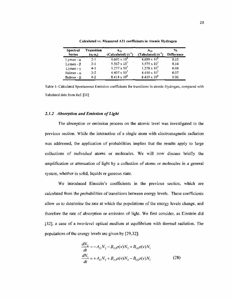
1. Calculated Spontaneous Emission coefficients for transitions in atomic Hydrogen, compared with Tabulated data from Ref. [31] 23

2. Parameters of the probed transitions in the Oxygen A-band, utilized for modeling (obtained from HITRAN [39]) 76

LIST OF FIGURES

ure Page

1. Evolution of the electron probability density function for an electric dipole transition in the Hydrogen atom (Is -> 2p° transition). The electronic charge distribution oscillates in a manner similar to a classical electric dipole antenna. While these figures illustrate absorption of a photon, the same behavior occurs (in reverse) during emission 20

2. Evolution of the electron probability density function for a magnetic dipole transition in the Hydrogen atom (Is -> 2p° transition). The electronic charge distribution rotates in a manner similar to a classical magnetic dipole antenna (e.g. current loop) 20

3. Molecular Orbital Structure of Oxygen 28

4. Potential Energy Curves in Molecular Oxygen, plotted vs internuclear separation 30

5. Oxygen A-band spectrum (Taken from HITRAN 2008 [39]) 35

6. Wavelength modulation spectroscopy signals (amplitude), for a Voigt absorption profile, for N=0 (direct absorption), and N=l through 5. The modulation index is m=3, and the amplitude modulation coefficient r = 0 (pure wavelength modulation) 45

7. Wavelength modulation spectroscopy signals, for a Voigt absorption profile, for N=l through 6. The modulation index is m=3, and the amplitude modulation coefficient r = 0.7 47

8. Illustration of non-uniform absorption across the transition frequency profile, with increasing penetration into the absorbing medium being probed. As the probe penetrates deeper into the absorbing medium, the absorption at linecenter is greater than in the wings. Thus, every element sees an input probe with a different profile than that of the preceding element 49

9. Pathlength saturation of the absorption profile with increasing optical depth. Since absorption at and near the linecenter is higher than in the wings of the profile, the linecenter saturates faster than the other regions. This leads to a broadening of the profile 50

XI

10. Pathlength saturation effects at higher harmonic wavelength modulation spectroscopy signals, at high optical pathlength of L=185m. The peaks at and around linecenter are suppressed at the higher harmonics (compare to Figure 6), an effect not present at direct absorption or lower detection harmonic orders. The signals are calculated for a modulation index of m=2.5... 52

11. Reduction of pathlength saturation effects at higher modulation indices, at pathlength of L=185m. When the modulation index is increased from m=2.5 to m=3.1, the peak suppression effect is reduced. In the case of N=6, the suppression is no longer easily discernable 53

12. Setup of experimental apparatus to perform WMS 65

13. Setup of experimental apparatus for Simultaneous Higher Harmonic WMS 69

14. Block diagram algorithm of phase-sensitive detection performed by a lock-in amplifier 71

15. Interface of Simultaneous Harmonic Detection program in Labview. Shown are the signals for N=4,5,6 and 7, obtained simultaneously in one sweep of the laser across the absorption profile 72

16. Comparison of harmonic signals obtained with a Stanford SR 850 (Blue) lock-in amplifier, against those obtained with a virtual simultaneous multiple harmonics lock-in amplifier on Labview. The quantity A is a measure of the cumulative percentage difference (absolute) between the two sets, with respect to the SR 850 system 74

17. Comparison of experimental (black lines) direct absorption signals with models assuming a Lorentzian (red lines) and Voigt (blue lines) profiles. Measurements were taken at pathlengths of (a) L=28m (b) L=68m and (c) L = 121m. The Lorentzian and Voigt models give nearly identical matches to the experiment 80

18. Fig. 18. Comparison of experimental WMS signals (black) with theoretical models using a Voigt profile (green) and a Lorentzian profile (red), as well as absolute differences (residuals) for the N=l,2...8t harmonic of the modulation frequency. The transitions being probed are oxygen A-band RR(13,13) and RQ(11,12) lines, with an optical pathlength of L=28m and a modulation index m=3.12. Insets are magnified portions of the data, illustrating the growing difference between experiment and the two models, sv and EL represent the mean absolute fractional deviations across the whole profile between theory and experiment, when modeling with a Voigt profile and Lorentzian profile, respectively. As is the percentage difference between

XII

Sv and 8L, with respect to ey 83

19. Mean Absolute Fractional Deviation between theory and experiment, when using Voigt and Lorentzian profiles, at various harmonics N of the modulation frequency. Error bars represent experimental uncertainty. As one goes to higher detection harmonic orders, the mismatch between theory and experiment increases. This makes any discrepancy between theory and experiment more pronounced at higher N, and therefore such measurements put a more stringent constraint on a model. In this particular case, it is also clear that (as would be expected under the experimental conditions) the Voigt is a better fit than a Lorentzian. However, it is harder to come to this conclusion at low N than at higher N 86

20. Comparison of experimental third harmonic WMS signals (black lines) with theoretical models using a Voigt profile (green lines) and a Lorentzian profile (red lines), for modulation indices of m=2.6 ((3=4.11 GHz), m=3.12 0=4.93 GHz) and m=4.18 (P=6.60 GHz). The optical pathlength, L = 28m 88

21. Comparison of experimental eighth harmonic WMS signals (black lines) with theoretical models using a Voigt profile (green lines) and a Lorentzian profile (red lines), for modulation indices of m=2.6 ((3=4.11 GHz), m=3.12 (p=4.93 GHz) and m=4.18 (p=6.60 GHz). The optical pathlength, L = 28m. The insets illustrate the decreased difference between models at higher modulation index 89

22. Fig. 22. Comparison of experimental WMS signals (black lines) with theoretical models using Voigt (green lines) and Lorentzian (red lines) profiles, for second (a), third (b), sixth (c) and eighth (d) harmonics at high pathlength of L=121m. (c) and (d) illustrate the suppression in peak that occurs at a modulation index of m = 3.12. The structure of the N=6 and N=8 signals are more accurately modeled when assuming a Voigt profile, while the Lorentzian model does not show a suppression of the central peak. While a depression is not directly visible at N=6, the pathlength saturation effect is still present: the peak of the RQ(11,12) line is lower than that of the RR(13,13) line (The same line has a higher amplitude at a lower pathlength as seen in previous figures, for example in figure (18f)) 91

23. Fig. 23. Reduction of pathlength saturation effect, when modulation index is increased from m=3.12 ((a) and (c)) to m=4.16 ((b) and (d)), in seventh and eighth harmonic signals at high pathlength of L=121m. While a depression is no longer visible at the higher modulation, the pathlength saturation effect is still present as a reduction of the peak heights 93

XIII

24. Experimental (black) direct absorption signals, compared with theoretical (green) model that includes the five labeled transitions, for pathlengths of L=68m ((a) and (b)) and L=121m ((c) and (d)). Figures (b) and (d) are magnified portions of the absorption signals in (a) and (c). Neither the experimental nor model data resolve the weak spectra, which are approximately two orders of magnitude weaker .......... 95

25. Experimental (black) and Theoretical (green) models, plotted on the full scale, for L= 121m and m=4.16, at (a) N=3 and (b) N=8. The weak transitions, which are not resolved at direct absorption or lower harmonics (e.g. N=3), are visible at N=8 97

26. Various harmonic signals between N=2 to N=8, on a 30X magnified scale, for L=121m and m=4.16. As shown, the weak spectra signals at N=8 are better resolved than at lower harmonics [ 98

27. Comparison of the resolution of weak spectra at (a) N=4, (b) N=5 and (c) N=6th harmonic of the modulation frequency, when the modulation index is increased from m=3.12 to m=4.16. The resulting modulation broadening causes a loss in the relative amplitudes and numbers of extra turning points that indicate the presence of the weak transitions 100

28. Shannon's simple communication system [11] 102

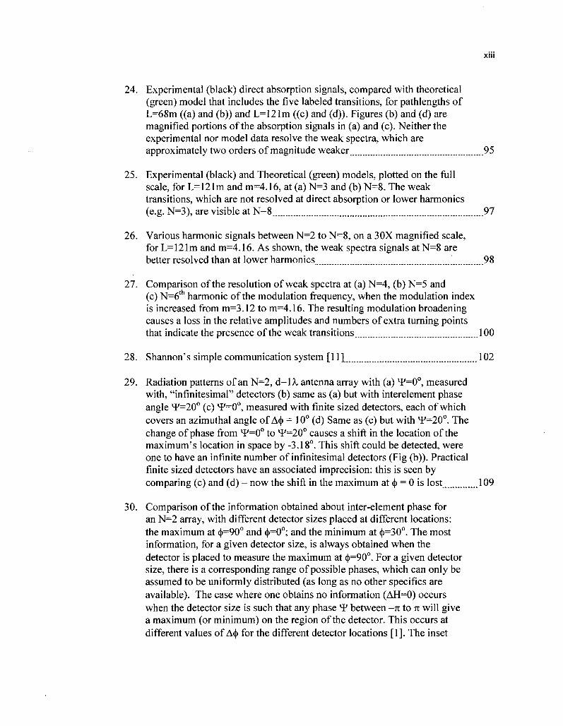
29. Radiation patterns of an N=2, d=lX antenna array with (a) ¥=0°, measured with, "infinitesimal" detectors (b) same as (a) but with interelement phase angle VF=20° (c) XF=0°, measured with finite sized detectors, each of which covers an azimuthal angle of A<j) =10° (d) Same as (c) but with ¥=20°. The change of phase from ¥=0° to 4/=20° causes a shift in the location of the maximum's location in space by -3.18°. This shift could be detected, were one to have an infinite number of infinitesimal detectors (Fig (b)). Practical finite sized detectors have an associated imprecision: this is seen by comparing (c) and (d) - now the shift in the maximum at (j) = 0 is lost 109

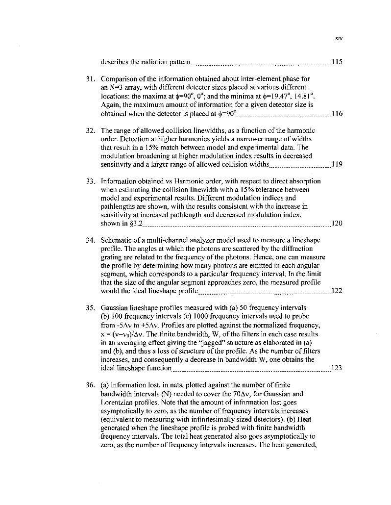
30. Comparison of the information obtained about inter-element phase for an N=2 array, with different detector sizes placed at different locations: the maximum at (j>=90° and §=0°; and the minimum at <j)=30°. The most information, for a given detector size, is always obtained when the detector is placed to measure the maximum at <))=90o. For a given detector size, there is a corresponding range of possible phases, which can only be assumed to be uniformly distributed (as long as no other specifics are available). The case where one obtains no information (AH=0) occurs when the detector size is such that any phase *F between -n to n will give a maximum (or minimum) on the region of the detector. This occurs at different values of A<|> for the different detector locations [1]. The inset

XIV

describes the radiation pattern 115

31. Comparison of the information obtained about inter-element phase for an N=3 array, with different detector sizes placed at various different locations: the maxima at <|>=90o, 0°; and the minima at <j>=19.47°, 14.81°. Again, the maximum amount of information for a given detector size is obtained when the detector is placed at <j)=90° 116

32. The range of allowed collision linewidths, as a function of the harmonic order. Detection at higher harmonics yields a narrower range of widths that result in a 15% match between model and experimental data. The modulation broadening at higher modulation index results in decreased sensitivity and a larger range of allowed collision widths 119

33. Information obtained vs Harmonic order, with respect to direct absorption when estimating the collision linewidth with a 15% tolerance between model and experimental results. Different modulation indices and pathlengths are shown, with the results consistent with the increase in sensitivity at increased pathlength and decreased modulation index, shown in §3.2 120

34. Schematic of a multi-channel analyzer model used to measure a lineshape profile. The angles at which the photons are scattered by the diffraction grating are related to the frequency of the photons. Hence, one can measure the profile by determining how many photons are emitted in each angular segment, which corresponds to a particular frequency interval. In the limit that the size of the angular segment approaches zero, the measured profile would the ideal lineshape profile 122

35. Gaussian lineshape profiles measured with (a) 50 frequency intervals (b) 100 frequency intervals (c) 1000 frequency intervals used to probe from -5Av to +5Av. Profiles are plotted against the normalized frequency, x = (v-vo)/Av. The finite bandwidth, W, of the filters in each case results in an averaging effect giving the "jagged" structure as elaborated in (a) and (b), and thus a loss of structure of the profile. As the number of filters increases, and consequently a decrease in bandwidth W, one obtains the ideal lineshape function 123

36. (a) Information lost, in nats, plotted against the number of finite bandwidth intervals (N) needed to cover the 70Av, for Gaussian and Lorentzian profiles. Note that the amount of information lost goes asymptotically to zero, as the number of frequency intervals increases (equivalent to measuring with infinitesimally sized detectors), (b) Heat generated when the lineshape profile is probed with finite bandwidth frequency intervals. The total heat generated also goes asymptotically to zero, as the number of frequency intervals increases. The heat generated,

XV

Q, is normalized to Q/Nohvo 126

37. (a) Heat generated vs. Information lost for the Gaussian and Lorentzian profiles. More heat is generated as the number of bits lost increases, (b) Heat generated per bit lost vs. the number of frequency intervals (N) used to measure the lineshape profile. The heat generated per bit lost follows a linear trend versus the number of intervals 127

1

CHAPTER I. INTRODUCTION

Every process of measurement inevitably leads to a perturbation of the medium

being studied. By measuring some property of a target, the measuring device ends up

distorting that target in some manner. This becomes particularly critical when one is

investigating highly sensitive phenomena, such as those on the atomic or molecular scale.

Thus, it has always been an important goal to find a method of measurement that

provides the least disturbance - fortunately, this is provided by light. Photons, being

massless, provide the "lightest touch" in many experiments, and absorption and emission

processes have become some of the most preferred sources of information for

characterization of any medium or process that absorbs or emits photons. One particular

application, for example, is the convenient characterization of a gaseous species by

probing its spectral absorption or emission profile.

Such methods have been successfully utilized to identify different species, and

make precise non-intrusive measurements of their temperature and velocity distributions,

pressure, density, and other physical parameters. Spectral techniques have even enabled

the study of the molecular and atomic structure of the gaseous medium being probed.

Optical sensing techniques furthermore allow one to probe regions that are unreachable,

such as terrestrial or higher earth atmospheres, or hostile environments. This allows for

many industrial applications, such as determination and control of reactants in a

processing environment, as would be necessary in microelectronics, for example.

Applications are also widespread in environmental monitoring and protection or national

Journal model used for this dissertation is Applied Physics B: Lasers & Optics

2

security, where the methods can be used for the detection of pollutants, particulate matter

or hazardous chemicals. Optical sensing methods provide a novel, precise, minimally

intrusive method for the investigation of gaseous substances.

The greater the precision of these measurement techniques, the faster the

advancements in industry and research utilizing these methods will be. However, often

times, such advancement is limited by the need to balance costs with accuracy.

Furthermore, certain apparatuses may or may not be compatible with the environment

they are intended for. Thus, there arises a need for different and efficient methods of

optical sensing. One such method, which is the focus of this research, is Wavelength

Modulation Spectroscopy (WMS), where a probing laser is modulated as it passes

through the target, and synchronous demodulation is performed at the receiving detector.

The advantage of this technique arises from the rich structure due to the derivative-like

behavior of higher harmonic WMS signals, resulting in turning points and zero crossings.

In this work, we develop a novel wavelength modulation spectroscopy method whereby

multiple harmonics are detected simultaneously, compared to previous sequential

detection methods. We investigate the sensitivity of WMS signals at higher harmonics to

differences in the theoretical modeling, and study the effects of modulation index and

high optical pathlengths on the ability to resolve spectra in atmospheric oxygen.

There are many questions that arise in such measurements. One such important

question, but less frequently asked, is "What is the maximum amount of information - in

bits - that one can extract from a measurement of some parameter?" An answer to this

question must first begin with the quantification of the amount of information in a

particular measurement. Understanding how to do so would allow one to optimize an

3

experimental setup for extraction of maximum information. We propose a method to

quantify the amount of information one obtains in such measurements, by investigating

radiation profiles in space and frequency.

1.1 BACKGROUND & MOTIVATION

Over the last couple of decades, the advent of diode lasers has resulted in a surge

in their use as optical probes in laser spectroscopy. In particular, their low cost,

compactness and tunability at various near-infrared and infrared wavelengths make them

ideal for probing gaseous molecules with vibrational-rotational transitions. Furthermore,

these lasers have generally stable operation at room temperature, are fiber-optic

compatible (allowing their light to be channeled to difficult-to-reach locations), and can

be easily tuned by adjusting the injection current or temperature. Due to these

advantages, among many others, semiconductor-based laser spectroscopy finds use in

many applications such as environmental monitoring, atmospheric sciences and materials

processing.

Over the last decade, one such application of diode lasers has been Wavelength

Modulation Spectroscopy (WMS). In WMS, the radiated frequency of the laser is

sinusoidally modulated. The signal on a photodetector, after the modulated beam passes

through a gaseous absorbing medium, is one that varies at the harmonics of the

modulation frequency, com. One can then demodulate the signal with a lock-in amplifier at

those harmonics of the modulation frequency, Noom. By doing so, one is able to eliminate

the majority of noise, except in a narrow bandwidth around the detection frequency. Such

techniques have been successfully utilized to study various gases and their properties, by

4

investigating the features of the WMS signals. Examples include, but are not limited to,

the measurement of temperature, line strengths, collision broadening and shock wave

effects in atmospheric oxygen [2-7], carbon dioxide [8-10] and hydrogen sulfide [11].

Most of these applications, however, have focused on the commonly used second

harmonic (2f) detection. It is well known that higher harmonic WMS signals provide a

greater degree of structure in the form of turning points and zero crossings, and can

therefore provide more sensitive probes for some of the above mentioned applications [2-

6]. However, the behavior of WMS signals is generally complex, and simply going to

higher harmonics is thus not always feasible. For example, higher harmonic signals have

a lower magnitude, and in the presence of noise would be difficult to resolve. This can be

countered by increasing the modulation index, but doing so broadens the signal, which

would cause loss of features as well. Thus, one has to find an optimal set of conditions

that allows for the maximum gain in information about the gaseous medium being

studied.

Furthermore, the previous methods have focused on a sequential collection of

data, where each harmonic signal is collected independently. This lends itself to

engineering difficulties, such as time-limitations and changes in the target that can occur

on the time-scales required for collection of each harmonic. Therefore, there arises a

necessity to develop detection apparatus that simultaneously collect signals at the

different harmonics. This eliminates uncertainties that would arise due to a changing

environment, which would otherwise be present when one performs sequential

measurements. In addition, the detection of various harmonic signals simultaneously may

possibly allow for a more efficient removal of distortions and noise. For example, when

5

one performs a particular series of sequential measurements N=l,2,3...8, each set of data

is associated with an independent noise pattern obtained at the time of each measurement.

However, if one utilized simultaneous detection of those eight harmonics, it is

conceivable that they would be able to more efficiently reduce the noise, since the noise

pattern would now be expected to be the same across the eight signals. This possibly

allows for a fundamental gain in information when using simultaneous instead of

sequential detection.

An aspect of the technique described in the references above that has not been

investigated before is the quantification of information that one obtains from a

wavelength modulation spectroscopy experiment. As every real measurement is

associated with some distortion, there is always an uncertainty in the quantity being

measured. For example, if one is estimating the temperature from the Doppler linewidth

of a spectral profile, then any uncertainty in the measurement of the profile will translate

to an uncertainty in the temperature. Such imprecisions in the measurement of the profile

would commonly arise from distortions due to noise or limited resolution of the

apparatus. This uncertainty can, however, be reduced by an improvement in the

apparatus, or by processing the data. According to Shannon [12-13], this reduction in

uncertainty can be quantified as a gain in the amount of information obtained about the

parameter being measured. Such quantification, as applied to radiation patterns in space

and frequency, as well as to WMS signals, has been described in references [1,14-19].

The work described in this dissertation investigates the use of simultaneous higher

harmonic wavelength modulation spectroscopy in the study of atmospheric oxygen [19].

In particular, we probe near-infrared optical transitions in the oxygen A-band.

6

Measurements of various line parameters of the oxygen A-band have been vital tools in

atmospheric sensing. For example, the Stratospheric Aerosol and Gas Experiment III

(SAGE III) instrument, which was a part of NASA's Earth Observing System of

satellites, used the oxygen A-band to measure temperature and pressure profiles of the

stratospheric and mesospheric levels of the atmosphere [20]. Likewise, the Atmospheric

Chemistry Experiment-Measurement of Aerosol Extinction in the Stratosphere and

Troposphere Retrieved by Occultation (ACE - MAESTRO) instrument, on the Canadian

SCISAT satellite, also utilizes the oxygen A-band to determine temperature and pressure

profiles in the atmosphere [21]. Hence, techniques to observe and accurately characterize

spectral profiles of transitions in the oxygen A-band play an important role in

atmospheric sensing.

The A-band is composed of transitions between the rotational energy levels of the

zeroth vibrational quanta (0 -> 0) of the ground electronic "triplet" state (X S~) to the

first excited electronic "singlet" state (b ~L+g). Transitions in this band are spin forbidden

and electric-dipole forbidden, but are magnetic dipole driven, making them fairly weak.

However, due to the high optical pathlengths available in the atmosphere, which enables

greater absorption by the species, the oxygen A-band transitions have been studied since

the early 1920s [22-23].

1.2 SUMMARY OF WORK DONE

We performed simultaneous wavelength modulation spectroscopy experiments on

transitions in the oxygen A-band, using tunable vertical cavity semiconductor emitting

7

lasers [5,19]. This involved modulating the injection current driving the laser, which

resulted in a wavelength modulation of the output of the laser. The beam was then passed

through a multi-pass cell based on the design of Altman [24], where the optical

pathlength could be varied. The output beam was then detected on a silicon photodetector

operating in the photoconductive mode, and the output signal was fed into National

Instruments Labview. A virtual Lock-In Amplifier program performs simultaneous phase

sensitive demodulation of the signal at multiple harmonics of the modulation frequency.

This additional element of signal processing makes WMS different from conventional

direct absorption spectroscopy, and provides additional structure that makes a WMS

signal sensitive to fine features that are otherwise difficult to detect. The experimental

data are then compared to theoretical models, which assume different lineshape profiles.

We find that higher harmonic WMS signals are sensitive to the type of lineshape profile

assumed in the theory, and allow one to distinguish between profiles that may not be

easily achievable with conventional spectroscopy. We investigate the effects of changing

the modulation index, as well as the optical pathlength, and discover features that allow

an even more sensitive probing of the lineshape profile.

A theoretical background is provided in Chapter II. We begin by reviewing the

interaction of light with matter by looking at a semi-classical treatment of the interaction

of an electric field with the hydrogen atom. We illustrate, through animations that were

obtained from quantum mechanical calculations, the behavior of the hydrogen atom when

it absorbs or emits a photon for different transitions. This is followed by a brief

discussion of the structure of the oxygen A-band, and we present a derivation of the

general equations of absorption of light by matter. A description of lineshape profiles that

8

we use in the theoretical modeling in this work is then provided. Finally, we describe the

theory of wavelength modulation spectroscopy, detailing the cases of pure frequency

modulation and frequency with amplitude modulation, as well as the effect of high

optical pathlengths.

Chapter III presents the experimental results, as well as theoretical modeling, of

the experiments done on two oxygen A-band transitions. We describe the development of

the simultaneous WMS apparatus, and present results comparing the output of our new

simultaneous detection mechanism to the previous sequential detection method. We then

investigate the sensitivity of WMS signals to the type of lineshape profile used in the

theoretical modeling, by matching the output of models to experimental data. We

investigate the sensitivity at different harmonics, as well as different optical pathlengths

and modulation indices, and suggest that higher harmonic detection allows for a more

sensitive characterization of the lineshape profile. Experimental results are also provided

that show higher harmonic WMS signals as a sensitive probe for the resolution of weak

spectra, that are otherwise not visible with direct absorption.

In Chapter IV, the quantification of information in distributions of photons in

space, as well as frequency, is discussed. First, the results of theoretical calculations for

the measurements of parameters in an antenna array by detecting its radiation patterns are

presented. The argument is extended to wavelength modulation spectroscopy signals, and

present results that suggest the rich structure of higher harmonic signals, which make

them more sensitive to changes in the parameters, allow for the extraction of more

information about those parameters. We conclude by providing a summary of our work in

Chapter V, and give a brief outline of the possible future direction of this work.

9

CHAPTER II. THEORETICAL DEVELOPMENT

2.1 THE INTERACTION OF LIGHT WITH MA TTER

2.1.1 Quantum Antennas

We begin by reviewing the fundamental theory behind the absorption or emission

of light by an atom. One fascinating consequence of our modern understanding of

quantum mechanics and electromagnetism (a field more properly described as quantum

electrodynamics), is the realization that the whole spectrum of electromagnetic radiation

is generated by the same process that governs the radiation from and reception by the

common antennas for radio and TV signals. This includes all wavelengths from the

ultrashort (with wavelengths in the sub-Angstrom range) such as gamma rays, x-rays,

ultraviolet and visible radiation, through infrared, microwave and very long wavelengths

(literally longer than thousands of kilometers).

Generally speaking, an antenna is a body that emits or absorbs electromagnetic

radiation. This definition makes every object an antenna, as every object will emit or

absorb electromagnetic radiation at some particular frequency based on its atomic,

molecular or crystal structure. This property of absorption and emission at a particular

frequency gives an element its "electromagnetic fingerprint." By studying the spectral

composition of the radiation that a body (essentially an antenna) emits, we can decode the

"fingerprint" and identify its composition - the well known technique of spectroscopy.

As the process of radiation depends on the atomic or molecular structure, we start by

studying the process at the lowest level possible, i.e. the atomic level. In this section, we

outline a calculation, using quantum mechanics, of the wavefunction of a Hydrogen atom

10

interacting with electromagnetic radiation. Having obtained the wavefiinction, we will

then produce plots illustrating the evolution of the probability density cloud of the

electron as the atom absorbs or emits a photon.

The concept of radiation in quantum mechanics involves the interference of

stationary states. These stationary states are stable "orbits" of the electron in an atom,

described by probability densities that are characterized by wave functions and energies.

As the electron transitions from one state to another, the difference in energy is related to

the absorption or emission of radiation, of frequency/ by hf = E2 -Ex; where E2 and Ej

are the energies of the upper and lower states, respectively, and h is Plank's constant. In

this process of "hopping" from one state to another, the electrons form a time-dependent

coherent interference state between the wavefunctions of the orbitals involved [25].

To appreciate the essence of this process, we will use a semi-classical approach

and consider the interaction of classically described electromagnetic radiation with a

quantum mechanical Hydrogen atom. While the case chosen is the simplest possible, the

physical understanding developed is easily extendable to more complex systems,

including the A-band of molecular oxygen studied in this dissertation. We apply time-

dependent perturbation theory with a small disturbance to the atom (in the form of

electromagnetic radiation), and then calculate, using quantum mechanics, the transition

probabilities between states involved in the emission or absorption of radiation.

Let us begin by considering the Hamiltonian of a freely orbiting electron in an

atom: H = h V(F), where p represents the momentum (and therefore kinetic energy), 2m

while V represents the potential energy. The Hamiltonian, in general, is an operator

11

related to the total energy of the system through an eingenvalue-eigenfunction equation

given by:

• •H-x¥(r,t) = E-*¥(r,t) (la)

where ^(rj) is the wavefunction of the electron, and ^(F,*)] gives the probability

density function of the electron.

Writing the momentum and energy operators explicitly gives us the more familiar

time-dependent Schrodinger equation (See, for example, Ref. [26-27]):

-—V2x¥(r,t) + V(r)*¥(r,t) = ih—¥(r,t) (lb) 2m dt

where the momentum operator is given by p = -/7?V and the energy operator E = ifidldt.

Solving (1), with the appropriate functional forms for the potential V, gives us the

wavefunction of an electron in an atom, which can then be used to determine the

probability density function and energies of the stationary states.

In the presence of electromagnetic radiation, however, the Hamiltonian will be

perturbed, giving:

H = H°+H' (2)

where H° is the stationary Hamiltonian in the absence of any disturbance (as given

above), and H' is the perturbing term due to the electromagnetic field. Note that when

writing the Hamiltonian as (2), we have assumed the contribution due to the disturbance

to be much smaller than the stationary Hamiltonian term. While this first order

approximation will be sufficient in understanding the behavior of an atom as it absorbs or

emits a photon, it only applies to cases where the interacting electromagnetic field has

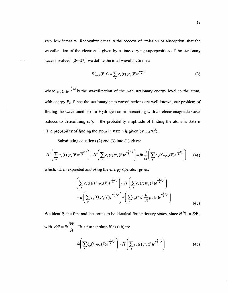
12

very low intensity. Recognizing that in the process of emission or absorption, that the

wavefunction of the electron is given by a time-varying superposition of the stationary

states involved [26-27], we define the total wavefunction as:

x¥,olal{r,t) = YJcM^'n{7)e,'E", (3)

where y/n (r)e h " is the wavefunction of the n-th stationary energy level in the atom,

with energy En. Since the stationary state wavefunctions are well known, our problem of

finding the wavefunction of a Hydrogen atom interacting with an electromagnetic wave

reduces to determining c„(t) - the probability amplitude of finding the atom in state n

(The probability of finding the atom in state n is given by \cn(t)\2).

Substituting equations (2) and (3) into (1) gives:

H° Zc»w^(F)e -EJ

\ " + H' ^cn{t)yy„{?)e » "'

v «

= ih-dt

E'UOV,, (*>"**"' V "

(4a)

which, when expanded and using the energy operator, gives:

( 5>B(0ff° ¥n{r)e

= ih

+ H' —EJ

IcB(/)f„(r)e h " V "

(4b)

We identify the first and last terms to be identical for stationary states, since H0x¥ = £ ¥ ,

with E?¥ = ih . This further simplifies (4b) to: dt

ih\ V "

Xc„(/)^(F)e"^"' =H\ YtCMvAryr**" (4c)

13

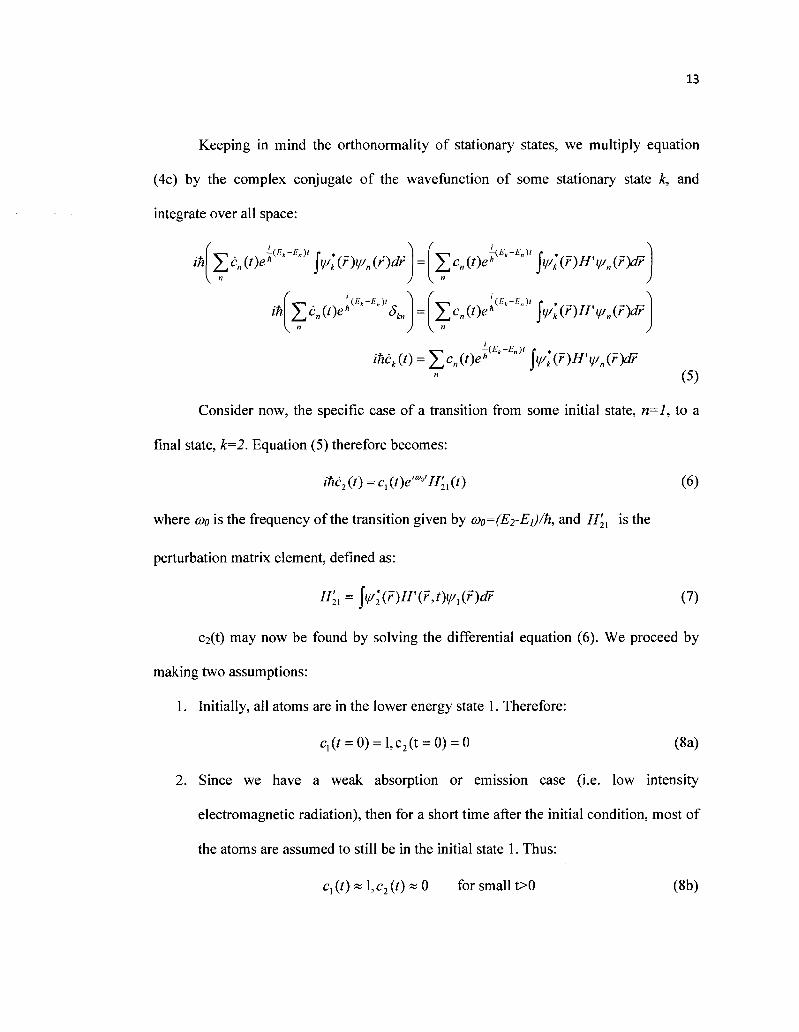
Keeping in mind the orthonormality of stationary states, we multiply equation

(4c) by the complex conjugate of the wavefunction of some stationary state k, and

integrate over all space:

\ f <• . . . . A

m £c„(Oe* (£ '" fn ) ' \w'k(r)ysn{r)dr = ^ M ^ " ' ^ ' \yk(r)H'y„(r)df , " J V "

ih

/ ^ ( 0 = XC«(0^ ( £ A"£" ) ' yk(r)H'rH(r)dr

V "

(5)

Consider now, the specific case of a transition from some initial state, n=l, to a

final state, k=2. Equation (5) therefore becomes:

ihc2(t) = c1(t)e/ao'H'2l(t) (6)

where coo is the frequency of the transition given by a>o=(E2-Ei)/h, and H'2l is the

perturbation matrix element, defined as:

H'2] = y2{r)H\7,t)yyx{r)dr (7)

C2(t) may now be found by solving the differential equation (6). We proceed by

making two assumptions:

1. Initially, all atoms are in the lower energy state 1. Therefore:

c,(/ = 0) = l,c2(t = 0) = 0 (8a)

2. Since we have a weak absorption or emission case (i.e. low intensity

electromagnetic radiation), then for a short time after the initial condition, most of

the atoms are assumed to still be in the initial state 1. Thus:

c, (0 « 1, c2 (0 * 0 for small t>0 (8b)

14

In light of these assumptions, equation (6b) reduces to:

c,{t) = ±-e,m°'H'n{t) (9) in

The solution of this simple differential equation, using the initial conditions (8a), is:

c2(t) = ±-)e""'H'2l(t')dt' (10) in 0

C](t) can be calculated from conservation of probability | cx(t)\ + \c2(t)\ -1. Knowing the

functional form of the perturbation Hamiltonian term, H'(f,t), we can determine c\(t) and

C2(t), as well as the total wavefunction T,^, (r,t).

As it stands, the above treatment is general and applies to any weak perturbation

on an atom that can be described by equation (2). We now proceed to determine H'(f,t),

for a specific case of interest to us: the interaction of electromagnetic radiation with an

atom. Assume that the atom interacts with a plane electromagnetic wave, described by

the magnetic vector potential:

A{r,t) = zA^sm{ky-(Ot) (11)

The total Hamiltonian of an electron in the presence of this field is given by [26-27]:

H=(p-qAf + F ( F ) ( 1 2 a )

2m

where q is the electronic charge. Expanding (12a), (being careful not to commute

operators):

2 21 J\2

H = ^- + V(r)—^-(p- A + A- p)+^-^- = H° + H' (12b) 2m 2m 2m

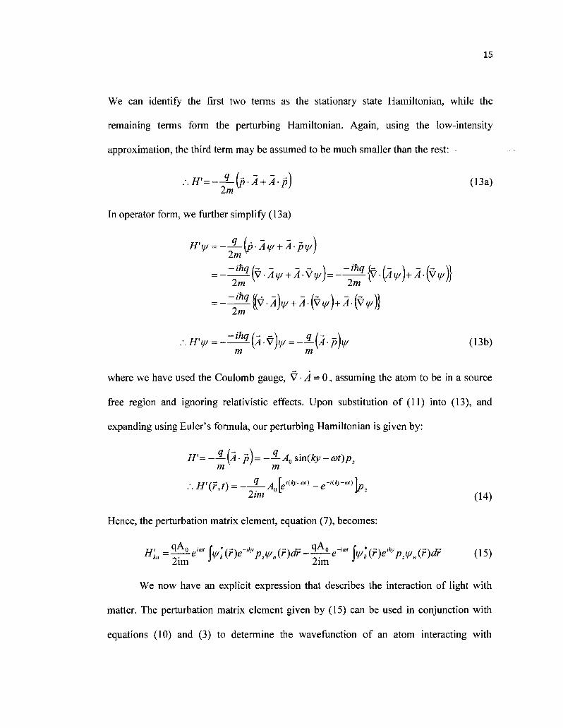
15

We can identify the first two terms as the stationary state Hamiltonian, while the

remaining terms form the perturbing Hamiltonian. Again, using the low-intensity

approximation, the third term may be assumed to be much smaller than the rest:

:.H'=-^-(p-A + A-p) (13a) 2m

In operator form, we further simplify (13a)

//'(// = ——\p-Ay/ + A-pi//) 2m

2m 2m

. • . / / y = _ Z ^ i ( ^ . v L = —?-(A-P)I// (13b) m m

where we have used the Coulomb gauge, V • A = 0, assuming the atom to be in a source

free region and ignoring relativistic effects. Upon substitution of (11) into (13), and

expanding using Euler's formula, our perturbing Hamiltonian is given by:

H'= -—[A pj= -—A0 sin(£y - coi)p. m m

:. H'(r,t) = —?-A0[e' l fy-a,) -e-^'^Xp, 2im ' (14)

Hence, the perturbation matrix element, equation (7), becomes:

H, = ^ e , „ yt(r)e-^p^m(f)dr-^-e^ yk(r)e^pziyn(?)dF (15)

2im J 2im J

We now have an explicit expression that describes the interaction of light with

matter. The perturbation matrix element given by (15) can be used in conjunction with

equations (10) and (3) to determine the wavefunction of an atom interacting with

16

electromagnetic radiation. While equation (15) is complete for describing the interaction

above, we expand the exponential term in the integral to further appreciate the emission

or absorption process:

Hi ~{e"* -e-m)\wl{7)p2wAr)dr

- - ^ ( * ' - +e-,")jV,,t(r)yplV,m{f)dr

+ higher order terms /1 /->

Let us examine the two terms separately. The momentum operator is related to the

stationary state Hamiltonian and position operators by the commutation relation [26]:

[z,HQ] = zU0-H0z = -pz (17) m

Substituting (17) into the first integral of (16), we obtain:

H^^^(eM -e-'-)yk(r)(zH0-HoZ)^(r)dr 2im ih J

= ~-(eM -e-*)yk(r)(zH0 -H0z)¥n{r)dr

= I ~ ( ^ -^)(E„ -Ek)yk(r)zvn(r)dr

= -i®oA sin(cDt)jt//l(r)qzi//n(r)dr

We also recognize that the electric and magnetic fields, in a source free region, are

related to the vector potential by:

r)A - -£ = - — , B = S7xA (19)

dt

Using equations (19) and (11), we can easily simplify (18) to:

# ' £ = - ' — £0sin(fflO(^k (20) CO

17

The term (qz)hl can be identified as an electric dipole moment oriented along the z-

direction [28]. Furthermore, the potential energy of an electric dipole in an electric field

is -p-E, where p is the electric dipole moment. Hence, the first term in the expansion

(16) corresponds to an electric dipole interaction between the electromagnetic wave and

the atom. Now consider the second term in (16), which we rewrite as:

qA0cos(cot)k r •,-.,( \ f~.r~

= - WkirnvPz ~zPy +yp, + zPyWn{r)df m J

2m J (21a)

The terms in parentheses of the first integral can be recognized as the x component of a

cross product of the position vector and momentum:

2m J

qA0 cos(fttf)A: r , \¥lir)Lxy/n(r)dr

2m J (21b)

where Lx is the x component of angular momentum. In addition, the amplitude of the

magnetic dipole moment of a current loop of area, a, and amplitude, /, is given by

fi = Ia = ——m1 = -*—mvr =-*—L . From (19), the amplitude of the magnetic field 2m 2m 2m

component of the electromagnetic wave in (11) is given by B0 = kA^. Therefore, equation

(21b) can be written as:

H'£a)=-B0cos(cot)(Mz)kn (21c)

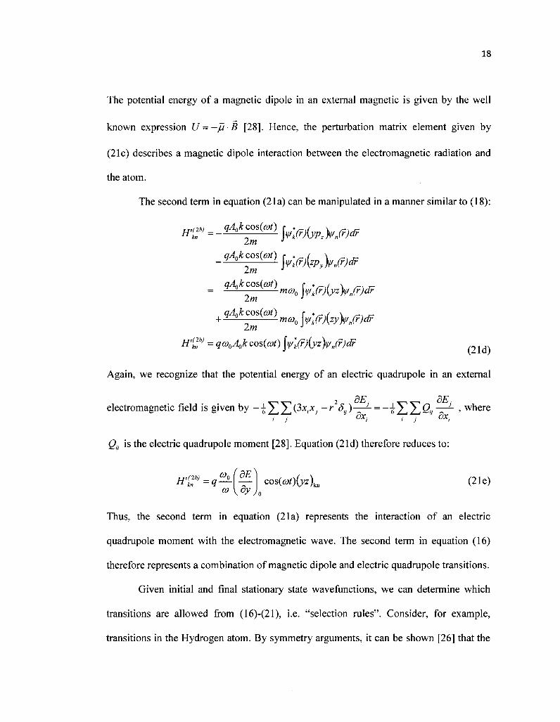
18

The potential energy of a magnetic dipole in an external magnetic is given by the well

known expression U--/1B [28]. Hence, the perturbation matrix element given by

(21c) describes a magnetic dipole interaction between the electromagnetic radiation and

the atom.

The second term in equation (21a) can be manipulated in a manner similar to (18):

TT,(2b> qA^kcosieot) r , , ^

2m J

— Wk(r)\zPykr,(r)dr 2m J

qA^kcosicot) r . / >. = — ^ ma>0\y/k(r)[yz)i/„(r)dF

2m J

+ — — mo)0 \xi/k(r)[zy}i/n(r)dr 2m J

H'Zb) = q®oA>k cos(flrf) jyr'k(r)(yz)f/„(r)dr ^

Again, we recognize that the potential energy of an electric quadrupole in an external

electromagnetic field is given by — jJ^J^Qx^j —r 8it)—- =-\'5\yy,QiJ—- > where i j fy i j dx,

Q0 is the electric quadrupole moment [28]. Equation (21d) therefore reduces to:

cos(<yO(j*L (2 1 e) n kn H ^dE^

CO

Thus, the second term in equation (21a) represents the interaction of an electric

quadrupole moment with the electromagnetic wave. The second term in equation (16)

therefore represents a combination of magnetic dipole and electric quadrupole transitions.

Given initial and final stationary state wavefunctions, we can determine which

transitions are allowed from (16)-(21), i.e. "selection rules". Consider, for example,

transitions in the Hydrogen atom. By symmetry arguments, it can be shown [26] that the

19

electric dipole transition, given by equation (20), vanishes except when A/ = ±1 and

Am = 0 (for a field polarized in the z-direction) or Am = ±1 (for a field polarized in x or y

direction); where / and m are the angular momentum and magnetic quantum numbers

respectively. Likewise, the selection rules for a magnetic dipole transition (equation

(21c)) are A/= 0 andAm = ± l , while the electric quadrupole transition (equation (21e))

requires A/ = 0,±2 and Am = 0,±1,±2 . The magnetic dipole and electric quadrupole

matrix elements vanish when the electric dipole matrix element is non-zero, and vice

versa (hence the commonly used term, "forbidden transitions," for the former two [26]).

The relative strengths of the different transition types can also be estimated from the

matrix elements, with the electric dipole being three orders of magnitude stronger than

the magnetic dipole and electric quadrupole transitions.

Examples of these transitions are illustrated in Figures 1 and 2 below, which plot

the evolution of the electron's probability density function during absorption of a photon.

Figure 1 is an electric dipole transition that occurs between the Is and 2p° states. Like a

classical electric dipole antenna, the probability density (i.e. "charge cloud") oscillates

vertically along the z-axis. Similarly, figure 2 illustrates a magnetic dipole transition that

occurs between the 2p° to 3p' state. In this case, the probability density undergoes a

rotation similar to a classical magnetic dipole antenna (i.e. current loop).

20

Fig. 1: Evolution of the electron probability density function for an electric dipole transition in the

Hydrogen atom (Is -> 2p° transition). The electronic charge distribution oscillates in a manner similar to a

classical electric dipole antenna. While these figures illustrate absorption of a photon, the same behavior

occurs (in reverse) during emission.

Fig. 2: Evolution of the electron probability density function for a magnetic dipole transition in the

Hydrogen atom (2p° -> 3p' transition). The electronic charge distribution rotates in a manner similar to a

classical magnetic dipole antenna (e.g. current loop).

21

An evaluation of the matrix elements also allows one to determine the Einstein

Rate coefficients (discussed in an upcoming section). From equation (15), the general

form of the perturbation matrix element may be deduced as H\n - axe~"°' + a2e'°" .

Substituting this expression into equation (10a) gives:

c2(t)«— \a,eKa°-m)' + a2e{m°+a)'dt

in 0

.-. c (t) = ai i\ - e'(^-»>}+ a* {l _ e^+a)l} (22)

In the limit that co -> coo, the second term rapidly oscillates to zero leaving one the

resonant first term. The probability of the upper state is therefore:

1 n{a)0-co) h{o)0-co) 2 2

{2-(e'Ao"+e-Alo')}= 2a ' 2{2-2cos(Ao)t)}

(23)

hl(Acoy " ' hz(Aco) , a ^ s i n ^ )

where ax = —3—5- w*k{r)p.y/n{r)dr for an electric dipole transition, and Aa> = coQ-co. 2im J

Note that the above probability is calculated assuming "sharp" energy levels, i.e. a

single, well-defined value of ©o. However, due to the Heisenberg uncertainty principle,

the energy levels are broadened and, as a result, there is a probability density g(coo) of the

transition frequency. Hence, the average probability [26,29-30] that the atom is in state 2

is given by:

22

. ,|2\ "ra, sin2(;r(v0-v)/) 2

7 0 fi (»"(vo-v)0

1 fsin(x)A

(JX. =-

h2

or, r 1 I sin(x) ) , a, , .

/I ' 7T\ X J (24)

The Einstein absorption coefficient, B12, is related to the rate of absorption

dN 2 [26,29-30] by — - = BnNlg(y)pv , where Nj is the population of state i andpv =j£E0

dt

is the energy density of the incoming electromagnetic radiation. Thus, we can equate the

occupation probability of N2 from this equation to (24), obtaining:

Bng(v)pj = ^^rg(y0)t

gi A- * (25)

where gi and g2 are the degeneracies of the two states. We obtain the Einstein

Spontaneous Emission coefficient, A21, from the relationship [26,29-30]:

A2l _ gx 8^7

Bn g2 A3

giving:

(26)

A» = 3Jf-ir (27)

A pv h

Table 1 presents A2i values calculated for some common transitions in atomic

Hydrogen, averaged across the / and m states for arbitrarily polarized electromagnetic

radiation [30]. The values are compared to tabulated data (from experimental and

astrophysical observations [31]), and are within 0.15%.

23

Calculated vs. Measured A21 coefficients in Atomic Hydrogen

Spectral Series

Lyman - a Lyman - P Lyman - y Balmer - a Balmer - p

Transition (nr i i i)

2-1 3-1 4-1 3-2 4-2

A21

(Calculated) (s"1)

4.692 x 10s

5.567 xlO 7

1.277 xlO 7

4.407 x 107

8.414 xlO 6

A21

(Tabulated) (s1)

4.699 x 108

5.575 xlO 7

1.278 xlO 7

4.410 xlO 7

8.419 xlO 6

% Difference

0.15 0.14 0.08 0.07 0.06

Table 1: Calculated Spontaneous Emission coefficients for transitions in atomic Hydrogen, compared with

Tabulated data from Ref. [31]

2.1.2 Absorption and Emission of Light

The absorption or emission process on the atomic level was investigated in the

previous section. While the interaction of a single atom with electromagnetic radiation

was addressed, the application of probabilities implies that the results apply to large

collections of individual atoms or molecules. We will now discuss briefly the

amplification or attenuation of light by a collection of atoms or molecules in a general

system, whether in solid, liquids or gaseous state.

We introduced Einstein's coefficients in the previous section, which are

calculated from the probabilities of transitions between energy levels. These coefficients

allow us to determine the rate at which the populations of the energy levels change, and

therefore the rate of absorption or emission of light. We first consider, as Einstein did

[32], a case of a two-level optical medium at equilibrium with thermal radiation. The

populations of the energy levels are given by [29,32]:

dN —L = -A2XN2- B2ip(v)N2 + Bnp{v)N, dt

^ = +A2lN2 + B2lp(v)N2 - Bnp(v)Nx (28)

24

where A21 is defined as the Einstein Spontaneous Emission Coefficient, B21 is the

Stimulated Emission Coefficient and Bn is the Absorption Coefficient. TV; and TV? are the

populations of the lower and upper energy levels respectively, while p(v) is the spectral

energy density of thermal radiation.

At equilibrium, the rate of change must be zero. Therefore:

^ = -A2lN2 - B2lp(v)N2 + Bl2p(v)N, = - ^ L = 0 at at

which results in

N2 _ Bnp(v)

TV, A2l + B2lp(v)

Since the system is at thermal equilibrium, we apply classical Boltzmann statistics:

(29a)

TV, ^, A2X +B2lp(v)

where g2 and gi are the degeneracies of the upper and lower states, respectively. From

(29b), we obtain:

p(v)- *21

BaM2_ei»i*T_B2i (30a) ^ 1

However, at thermal equilibrium, the spectral energy density is given by the well known

expression of Planck [29]:

87TV2 hv p(y)= cs e*w_x ( 3 0 b )

We can therefore obtain relationships between the three coefficients:

25

B2l c3 B2l gx

which we used in our determination of the spontaneous emission coefficient from

transition matrix elements (equation (26)). The above approach was initially used by

Einstein to determine the spectral energy density of blackbody radiation [32].

Let us now consider interaction of the medium with a coherent light source, i.e. a

laser, instead of thermal radiation. The spectral width in this case is very narrow and may

therefore be approximated by p(v)« pyS(v'-v), where pv is the energy density of the

probing beam. Furthermore, we note that since the energy levels are not "sharp" as

described above, the absorption or emission frequency v must instead be defined by a

probability density g(v). Hence, the rate equations (28), averaged over this probability

density and narrow spectral width become [29]:

dN —^ = -A2lN2 - B2lPvg(v)N2 + Bl2pvg{v)Nx (32)

at

The energy density of electromagnetic radiation ispv= I/c, where / is intensity. From

(32), we can now determine the change in intensity of light as a result of the change in

population, in a segment of the medium of length dz and area .4:

dN., hvAdz d ^T hvAdz 1 dQ. „ , . „ hvAdz „ , WT hvAdz — = ~A^i — - - " B2lPvg(v)N2 — — + Bl2pvg(v)Nx

dt A " * A 2 An "' " ~ ' ' A " ' ' " v ' ' A

2 ~dI = --\ AotN, ^ ^ )dz - - hvg(v){B21N2 - Bl2Nx )dz

dl hv

An

( n \ = — g(v)B2i N2--^NX

dz c

5,.

V 5 21 J

\( . „ hvdCi , + 2 \ A " N ' ^

26

The second term above can be considered "noise" due to its random nature, and we

disregard it since the work described in this dissertation focuses on absorption processes.

Thus, substituting (31) into the above expression, we obtain:

dz

(

N2-^-Nx g

i=°M i J

N,-&-N, g i J (33)

where ast(v) is defined as the stimulated emission cross section. An alternate use of the

00

cross section is in terms of the integrated cross section, defined as a = \a(v)dv , which 0

leads to <r(v) « (fg(v).

Equation (33) is a fundamental expression in any process that involves the

absorption or emission of light by matter. Assuming the density of the upper state to be

much smaller than the lower state, we can obtain the important absorption equation:

^- = -Nl(Jabs(v)I = -N1ag(v)I dz (34)

where aabs(v) is the absorption cross section, related to the stimulated emission cross

section by aabs(v) = g21gxa„(v).

2.2 SPECTROSCOPY OF THE OXYGEN A-BAND

The absorption or emission of light by matter was presented in the previous

section, with particular application to atomic Hydrogen. The physics of interaction

between light and matter composed of many atoms, however, is essentially the same, and

the above approach may be extended to molecules. All that is required is a sufficient

understanding of the structure of molecular energy levels. In this section, we review the

27

molecular structure of diatomic Oxygen. We briefly discuss electronic, vibrational and

rotational energy levels, with specific application to Oxygen A-band spectroscopy.

The first analyses of the Oxygen A-band were carried out by Mulliken [22,33-35],

mostly under the Born-Oppenheimer approximation. Under this approximation, the

electronic motions in a molecule are assumed to be much faster than the nuclear (i.e.

vibrational and rotational) motions. Hence, the total molecular wavefunction can be

decomposed into a product of the wavefunctions of the individual components. In this

manner, we can analyze the electronic, vibrational and rotational transitions separately,

and then sum the individual energies to calculate the absorption or emission lines.

2.2.1 Electronic Energy Levels in Molecular Oxygen

We begin by reviewing the electronic energy structure of molecular oxygen. The

ground state electronic distribution of atomic oxygen is given by (ls)2(2s)2(2p)4. When

two oxygen atoms bond, forming a diatomic molecule, the s-orbitals from each atom

form a bonds, while the three p orbitals form a a bond and two it bonds [36-38]. Let us

examine this latter statement by expanding the p-orbital configuration into its degenerate

states: (2p)4= (2px)2(2py)'(2pz)

1. If we define the inter-nuclear axis as oriented along the

z-direction, the two pz orbitals combine to form a a bond, while the px and py orbitals

form 7ix and ny bonds, respectively, a orbitals may be occupied by a maximum of two

electrons, while a degenerate n orbital can be occupied by up to four electrons.

In addition, according to molecular orbital theory, the coherent wavefunction of

all bonds can form with an addition or subtraction of the individual wavefunctions, i.e.

28

y/± = A ± B where A and B are the wavefunctions of the individual atoms [38]. Thus, one

obtains a bonding (+) or antibonding (-) orbital of each type mentioned above.

Furthermore, for homonuclear diatomic molecules, every bond is specified by its

inversion symmetry - that is, whether the wavefunction exhibits symmetric or

antisymmetric behavior when it is inverted through the molecule's center [36-38]. The

notation for inversion symmetry is a "g" (from the German word "gerade," meaning

even) for even symmetry, and "u" (from the German word "ungerade," meaning uneven)

for odd symmetry. The detailed structures of the different bonds, as well as higher order

bonds, are discussed thoroughly in references [36-38].

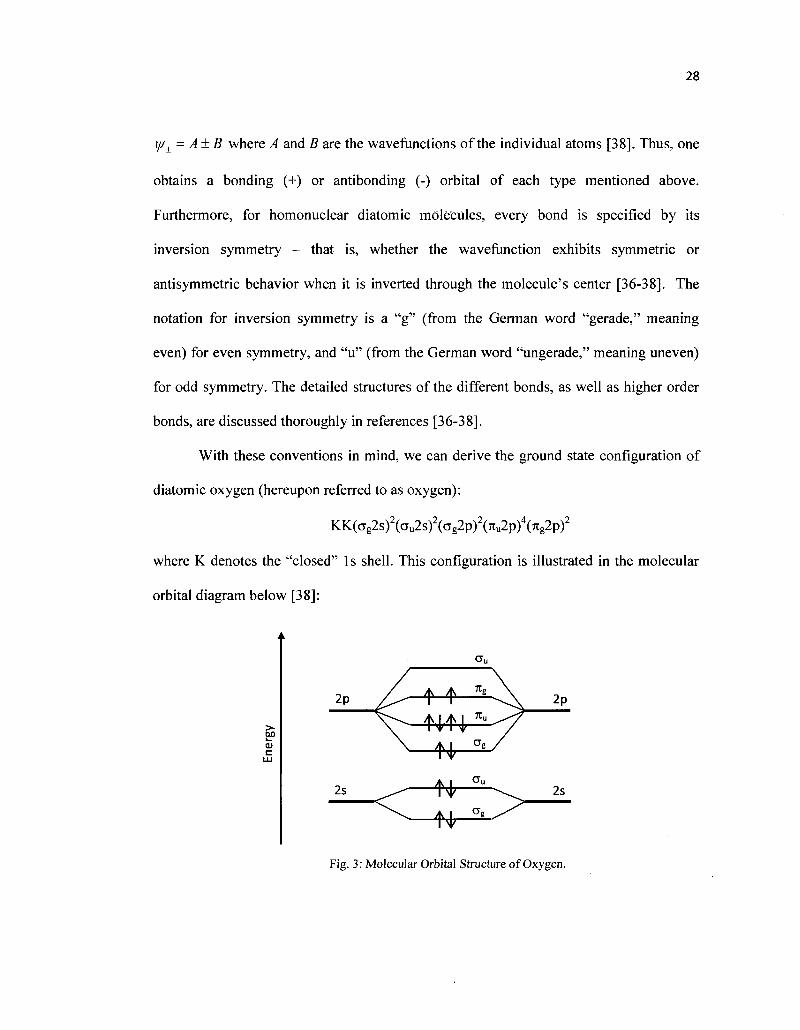
With these conventions in mind, we can derive the ground state configuration of

diatomic oxygen (hereupon referred to as oxygen):

KK(ag2s)2(au2s)2(ag2p)2(7iu2p)4(7ig2p)2

where K denotes the "closed" Is shell. This configuration is illustrated in the molecular

orbital diagram below [38]:

00

2s 2s

Fig. 3: Molecular Orbital Structure of Oxygen.

29

The two 7rg electrons in the open shell can lead to three configurations, giving

three different values for the total angular momentum quantum number, A [36-38]. The

two electrons may occupy different ng orbitals, with parallel spins, as shown in Figure 3,

with one in the 7igjX orbital and the second in the n&y orbital. This configuration leads to a

total angular momentum A = 0 (defined as the E energy level) and total spin S = 1

(defined as a triplet state). Another configuration involves both electrons in the same ne

orbital (Tcgx or 7igy), with antiparallel spins. In this case, A = 2 (defined as a A energy

level) and S = 0 (defined as a singlet state). The third configuration is the two electrons in

different orbitals, but with antiparallel spins; leading to A = 0 (E energy level) and S = 0

(singlet).

Thus, the three lowest configurations in oxygen are IT, Ag, £*. By Hund's

rule, the 3E~ state has the lowest energy and is therefore denoted as the ground state [36].

The oxygen A-band is one of four atmospheric absorption bands in molecular oxygen,

formed from transitions between the triplet E~ (ground) state and the singlet Eg

(excited) state: 3E~ -> E* . The four different bands arise from transitions between the

rotational states of different vibrational energy levels of these two electronic states. The

bands are labeled: A(0-»0), B(0^1) , y(0-»2), and 5(0->3), where (v '-*v") implies a

transition from the vibrational level v' of the lower electronic state to the vibrational level

v' of the upper electronic state; and the preceding letter denotes the band. Transitions

such as these involving changes in electronic, vibrational and rotational states are termed

rovibronic [36].

30

The two electronic energy levels are separated by approximately 13121 cm" [37]

centering the A-band at approximately 762nm. The transitions are electric dipole

forbidden and spin-forbidden, owing to the differences in symmetry and degeneracy.

They are instead, magnetic dipole driven, similar to the transition described in Figure 2,

making the absorption very weak. In addition, an electron must change its spin during the

transition, making the A-band lines even weaker. The potential energy curves of

molecular oxygen are given in Figure 4 below, illustrating A-band transitions.

80,000

60,000

t ~ 40,000

m

20,000

0

1 2 3 rxl^em—*-

Fig. 4. Potential Energy Curves in Molecular Oxygen, plotted vs internuclear separation.

2.2.2 Vibrational and Rotational Energy Levels

In addition to electronic energy levels, molecules are characterized by vibrational

and rotational energy levels. As can be seen in Figure 5, the minimum energy does not

occur at a single, "fixed," internuclear separation, but instead over some finite range of

values. The separation can only be defined to some finite precision, limited by the

Heisenberg Uncertainty Principle ApAx > h. As a result, the minimum energy is quantized

Oxygen A Band Transitions

31

at some level within the potential curve, constrained by a balance of uncertainty in

position and momentum.

The vibrational motion of diatomic molecules can be analyzed as a quantum

mechanical harmonic oscillator, i.e. mass and spring system. The allowed energy levels

of molecular vibrations, which fall within the potential wells (Figure 4), are then

approximately given by [36-37]:

Evtb=hco-(v + ^j (35)

where v is the vibrational quantum number and co = KI mr is the fundamental vibration

fti in frequency. Here, mr = —•—— is the reduced mass of the system, while K is the force

m] +m2

constant (i.e. "spring constant"), obtained from the molecular interaction potential. To

first order, we assume that the two atoms are bound by electrostatic attraction, given by

the Coulomb force [37]:

F=_}_(Mk (36a)

where Qj are the charges of the atoms in the molecule, and re is the equilibrium distance

between the atoms. However, it is also well known that the restoring force of a spring-

mass system is given by:

F = -K{r-re) dF (36b)

=>*: = dre

Equating (36a) and (36b), the force constant is therefore approximately:

32

*•-2-££ (37)

Note that the harmonic oscillator approximation, described by the evenly spaced

energy levels given in equation (35), is only valid for the low vibrational quantum

numbers, v. As can be seen from the potential curves in Figure 4 of a real system, the

higher energy levels (i.e. higher vibrational quantum numbers) are associated with

anharmonic oscillations. In this limit, the spacing between the energy levels continually

decreases as v increases, until the vibrational energy is high enough to cause dissociation

of the molecule. In the Oxygen A-band, however, transitions are between the lowest

vibrational energy levels, (0->0), and the harmonic oscillator approximation is therefore

sufficient.

At these low vibrational energy levels, we can also assume that the equilibrium

separation of the atoms is much larger than the distance over which the molecule

vibrates. Therefore, the radial motion can be approximated, to first order, by a rigid rotor

with energy levels [36]:

h2

ER= — J(J + \) = BhcJ(J + 1) (38)

where J is the rotational quantum number, / = jur2 is the moment of inertia, and B is the

rotational constant. The above approximation assumes that the two masses are held

together by a rigid massless bar. A better approximation, when considering the

vibrational motion, is the two mass points held together by a spring. In this latter case,

however, the internuclear distance, and therefore the moment of inertia, increases with

33

increasing rotation (as a result of the centrifugal force). Thus, a better description of the

rotational energy levels is [33,36]:

ER=BhcJ(J + l)-DhcJ2(J + \)2 (39)

where the rotational constant D = 4B3 la1. It should be noted that some authors define

the second order term with an addition, opting to define D as a negative of the above. The

values of B and D determine the spacing between rotational energy levels in a particular

vibrational rung.

We can now determine the total energy by combining the electronic, vibrational

and rotational energies:

^T = & electronic + -^vib + ^ R

~ ^electronic + "& ' v + - ] + BhcJ{J +1) - DhcJ2 (J +1)2

2 J (40)

2.2.3 Oxygen A-Band Transitions

Every transition between different energy levels is associated with selection rules.

The change in vibrational quantum number, v, can take any value i.e. Av - 0,±1,±2,...

However, intensities of the different vibrational transitions vary due to differences in

probabilities, dictated by the Franck Condon principle [36]. The oxygen A-band is

associated with the v'=0 -> v"=0 vibrational transition.

The total angular momentum is N=J+(A+S), where J is the rotational quantum

number, A is the orbital angular momentum quantum number and S is the spin quantum

number. This quantity changes by AN = 0, ±1 and the three possible cases are designated

"P" for AN = - 1 , "Q" for AN = 0 and "R" for AN = +1. Additionally, the rotational

34

quantum number can change by AJ = ±1, with a similar designation of P for AJ = - 1 ,

and R for AJ = +1. These transitions are forbidden by electric dipole criteria, but are

allowed by a magnetic dipole coupling of the electromagnetic field with the molecule.

Hence, A-band transitions are very weak and require relatively large pathlengths to be

observed.

From this set of selection rules and equation (40), the A-band therefore has two

branches about E'electromc-E"eleclmnic (X3S~ ->blI.+g). Note that AA = 0 for this transition.

The P-branch of the band is of lower energy, while the R-branch is higher. Transitions

are labeled with the notation:

AJAN(J",N")

where

AJ = J AN = <! 1 + 1 R

-1 P

0 Q + 1 R

and J", N" are the quantum numbers of the lower state. Consider, for example, the

RQ(11,12) absorption line. This implies a transition between J= 11 -> 12, N=12->12.

Likewise, the RR(13,13) line (another line probed in our work) involves a transition

between J=13-> 14, N=13->14. We determine from this that the total spin change is

S=l->0 during the RQ(l 1,12) transition, and S=0-»0 during the RR(13,13) transition.

Figure 5 illustrates the different transitions of the A-band, with line parameters

from the HITRAN database [39].

35

R-branch P-branch

•iifflii'i i i i iuumui ii .li i l • • • • :

759.0 "60.0 761.0 752.0 763.0 764.0 765.0 7S6.0 7S7.0 7« .0 '69.0 770 .C

Waveteiigtb [uifl]

Fig. 5. Oxygen A-band spectrum (Taken from HITRAN 2008 [39]).

2.3 THEORY OF WA VELENGTH MODULATION SPECTROSCOPY

Wavelength modulation spectroscopy involves the modulation of the frequency of

a probing laser, which then traverses an absorption medium, followed by synchronous

detection at the output. As we will see below, wavelength modulation spectroscopy

provides additional features that are not always discernible in conventional "direct

absorption" spectroscopy, making it advantageous over other spectroscopic methods in

certain applications. The frequency modulation of a laser can be achieved by many

different methods. Some of these techniques are capable of creating pure frequency

modulation in the probe beam, while others generate a "parasitic" amplitude modulation

in addition to the frequency modulation.

36

One method of performing wavelength modulation spectroscopy is by the use of

electro-optic phase modulators or external cavity lasing systems. External cavity lasers

are designed with a laser diode or lasing dye medium, with a high-reflection coating on

the back face and an anti-reflection coating on the front face. The feedback for laser

oscillation is then provided in an external cavity by using a diffraction grating, such as in

the Littrow configuration, or with a combination of a mirror and diffraction grating, as in

the Littman-Metcalf configuration [40]. The wavelength of the laser is then tuned, and

thereby also modulated, by rotating the diffracting grating or mirror, making this type of

laser capable of pure frequency modulation. External cavity lasers, however, require an

extremely high quality anti-reflection coating resulting in a high cost. In addition, the

accuracy of modulation depends on the mechanical precision of the device (such as a

motor) rotating the diffraction grating. This makes them preferable only in cases where

the species being investigated has very low absorption and therefore requires highly

sensitive apparatus.

Semiconductor lasers are another method commonly used for wavelength

modulation spectroscopy, as their frequencies can be easily controlled and modulated by

changing the temperature and injection current. Furthermore, their relatively low cost,

smaller sizes and fiber optic compatibility make them advantageous over their bulkier

and more expensive counterparts. However, injection-modulated lasers are one of the

sources associated with the parasitic amplitude modulation.

In this work, we have utilized Vertical Cavity Surface Emitting Lasers (VCSELs).

Briefly, a VCSEL is a semiconductor laser where the light emitted is perpendicular to the

surface. A thin semiconducting material of high gain, such as quantum wells, acts as the

37

lasing medium and is sandwiched between two highly reflective mirrors. These mirrors

may be dielectric multilayered mirrors, or distributed Bragg reflectors, capable of a

reflectivity greater than 99.9%. In addition to being smaller and more cost-effective than

edge emitting semiconductor lasers, the unique design of VCSELs provides narrow beam

divergence, low power consumption, high tunability and modulation bandwidth, and

better polarization control [41]. VCSELs also offer the possibility of making large,

compact arrays of coherent light sources [42]. Being injection current-driven lasers, we

must however keep in mind the amplitude modulation that accompanies the wavelength

modulation when developing a theory of WMS experiments that utilize VCSELs.

The frequency of a sinusoidally modulated laser [6,43] can be described by

v(/) = vL +J3coso>mt, analogous to frequency modulation in communication systems.

Here com is the modulation frequency (in radians per second), f3 is the amplitude of the

swing in frequency and vL is the frequency of the laser. In wavelength modulation

spectroscopy, the laser frequency is very slowly tuned over some wavelength range of an

absorption line. The period of this ramp, Tramp, is much greater than that of the

modulation, i.e. T » 2nl com. The ramped, modulated beam is then passed through an

absorbing medium. Coherent detection is then performed at the output, where the

absorption signal is demodulated at harmonics of the modulation frequency using a lock-

in amplifier. One advantage of this technique is a reduction in noise, because the

detection performed by the lock-in amplifier is in a narrow bandwidth around the N-th

harmonic frequency (which is usually higher than the 1/f type base-band noise of the

laser).

38

In this section, we will use these concepts to develop the theory of wavelength

modulation spectroscopy with tunable diode lasers. We will first derive the WMS signal

as a Fourier component at the harmonic N, using Wilson's method. While this model

gives us good agreement between experiment and theory, we will also investigate the

WMS signal under a weak absorption approximation, utilizing the Taylor series

expansion. This latter approach allows us to discuss the structure and variation of the

signal under different parameters (such as the modulation index and detection order). We

will also address in our models the simultaneous amplitude modulation that accompanies

the frequency modulation, as well as the slow ramp as the probing beam is swept across

the absorption spectrum. Finally, we will discuss a unique, novel feature in wavelength

modulation spectroscopy that occurs at high absorption lengths: pathlength saturation.

2.3.1 Wilson's Method

Consider first a conventional "direct absorption" spectroscopy experiment: A

laser probe beam passes through an absorbing medium, and is then measured on a

photodetector. The intensity through an infinitesimal segment of this medium is given by

equation (34), also known as the Beer-Lambert law:

~ = -nag(v)I = -a(v)I (41)

az

where n is the density of the lower state, a is the integrated absorption cross section and

g(v) is the lineshape function of the transition being probed. Assuming that the absorption coefficient a(v) = nag(v) is independent of intensity, the signal on a

photodetector after the beam traverses an absorbing medium of length L is given by:

39

I(v) = I0cxp[-nag(v)L] (42)

where Io is the initial intensity of the beam prior to entering the medium.

When the probe is frequency (wavelength) modulated, the lineshape function

depends on the probe frequency as g(v + ft cos coj) . Thus, the intensity on the

photodetector in a WMS experiment with pure frequency modulation is given by:

I(v + P cos co J) = I0 exp[-naLg(v + j5 cos coj)] (43a)

Because this function is periodic in com, we expand it in a Fourier series:

00

I(v + p cos coj) = £ Sm (v) cos(mcomt) , m = 0 *• '

In synchronous detection, the signal is demodulated at some harmonic, N, of the

modulation frequency. In our experiment, a lock-in amplifier mixes and filters the signal

from the photodetector with a sinusoidal signal of frequency Ncom, effectively producing

harmonic detection signals that are proportional to the N-th harmonic Fourier series

coefficient. The N-th harmonic WMS signal is therefore given by [44]:

1 " SN=— \l(y + j3 cos 9) cos(N0)dd (44)

71 -i

with 6 = coj . This cosine term of the Fourier series corresponds to the "x-signal" in a

lock-in amplifier. If the harmonic signal is determined from the sine term, we obtain the

"y-signal". In our work, we measure the amplitude of the signal, i.e. the "R-signal", equal

to the magnitude of equation (44).

In diode lasers, both the wavelength and intensity get modulated when the

injection current is modulated [6,19]. Therefore, equation (43a) is not sufficient to

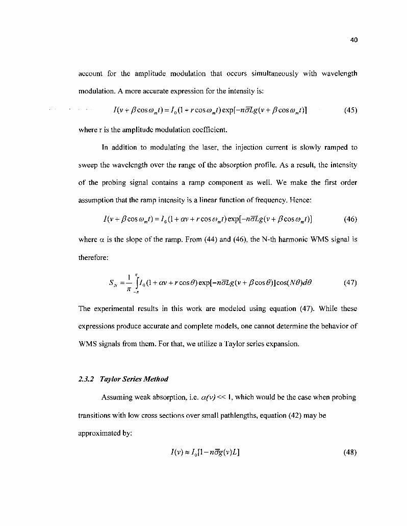
40

account for the amplitude modulation that occurs simultaneously with wavelength

modulation. A more accurate expression for the intensity is:

I(v + (5 cos co>J) = 10(1 + r cos co J) exp[-naLg(v + (3 cos co J)] (45)

where r is the amplitude modulation coefficient.

In addition to modulating the laser, the injection current is slowly ramped to

sweep the wavelength over the range of the absorption profile. As a result, the intensity

of the probing signal contains a ramp component as well. We make the first order

assumption that the ramp intensity is a linear function of frequency. Hence:

I(v + /3 cos comt) = I0 (1 + ccv + r cos coj) Qxp[-naLg(v + /?cos coj)] (46)

where a is the slope of the ramp. From (44) and (46), the N-th harmonic WMS signal is

therefore:

1 n

SN=— \lo(l + av + rcos0)exp[-naLg(y + /3cos0)]cos(N0)d0 (47) -71

The experimental results in this work are modeled using equation (47). While these

expressions produce accurate and complete models, one cannot determine the behavior of

WMS signals from them. For that, we utilize a Taylor series expansion.

2.3.2 Taylor Series Method

Assuming weak absorption, i.e. a(v)« 1, which would be the case when probing

transitions with low cross sections over small pathlengths, equation (42) may be

approximated by:

7(v)*/0[l-/i5j(v>I] (48)

41

From (44), the detected signal at the N-th Harmonic is:

1 " SN =- \lo[l-naLg(v + /3cos0)]cos(N$)dO

- -n -

= -naLI± {g{y + pcose)co^N9)de (49)

Using a Taylor series expansion about v, Myers and Putzer have shown [6,45] that the N-

th term of the Fourier series expansion of g(v + J3cos(comt))'m equation (49) is given by:

m=o ml V2/ , K»,-N (50)

where Bmm_N is the coefficient of the zm'N term in the expansion (z2 -\)m , z = e'* , and

where the residue theorem has been used. Therefore, from equations (49) and (50), the N-

th harmonic WMS signal is given by [6]:

SN =-naLIa{-\rvif{£\m+N 1 g2m+N(v) (51) til) m\{m + N)f

Here, [N]=N for even harmonics and [N]=N-1 for odd harmonics, and g2m+N(v) is the

(2m+N)-th derivative of the lineshape function.

For small modulation amplitudes, i.e. small (3, the m=0 term dominates, and it can

be seen that the N-th harmonic signal SN is proportional to the N-th derivative of the

lineshape profile. It is this feature of N-th harmonic WMS signals that gives them the

structure of (N+l) turning points and N zero crossings.

While this derivative signal is a good first order approximation, accurate

modeling requires a large number of terms in the expansion. This leads to possible

convergence problems depending on the functional form of the g(v). Furthermore,

42

regardless of how many terms one includes in the expansion when modeling, equation

(51) is insufficient, as it does not include amplitude modulation effects.

We will now include those effects. Recall from equation (45) that the intensity in

the presence of amplitude modulation is given by:

I(v + P cos coj) -10 (1 + r cos coj) Qxp[-naLg(v + /? cos coj)]

Again, assuming weak absorption, i.e. naLg(v0)«l, the intensity incident on the

detector is [6]:

I(v + ft coscoj) = IJ\-rioLg(v + P coscoj) Terml

+ r cos coj. Term 2

-rrioLg cos (coj) (v + /? cos coj)J Term 3 ^y\

When performing phase-sensitive detection (with a lock-in amplifier, for instance), Term

1 corresponds to the case of pure wavelength modulation. Term 2 contributes a constant

r/2 at the first harmonic, while Term 3 is the additional contribution due to the amplitude

modulation at all harmonics. As expected, one obtains the pure frequency modulation

case when r=0.

In order to evaluate the WMS signal, the same approach as that in obtaining

equation (50) is used. The components of the N-th harmonic signal from (51) are given

by:

oo

Term 1 => -noL( - \f]n £ f(N,fi, m) (53) m=0

Term 3 => -rnoL

"w'I+i

fdf(N-\,p,m)-Ydf(N + \,P,m) m=0(N>\)

(54)

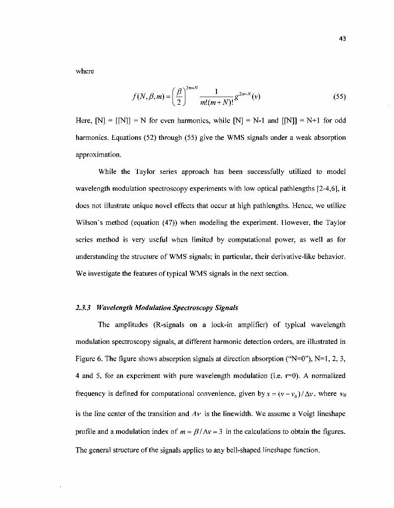
43

where

f a\2m+N

1 f{N,P,m)= Z- g — (v) (55)

\2) m\(m + N)\

Here, [N] = [[N]] = N for even harmonics, while [N] = N-l and [[N]] = N+l for odd

harmonics. Equations (52) through (55) give the WMS signals under a weak absorption

approximation.

While the Taylor series approach has been successfully utilized to model

wavelength modulation spectroscopy experiments with low optical pathlengths [2-4,6], it

does not illustrate unique novel effects that occur at high pathlengths. Hence, we utilize

Wilson's method (equation (47)) when modeling the experiment. However, the Taylor

series method is very useful when limited by computational power, as well as for

understanding the structure of WMS signals; in particular, their derivative-like behavior.

We investigate the features of typical WMS signals in the next section.

2.3.3 Wavelength Modulation Spectroscopy Signals

The amplitudes (R-signals on a lock-in amplifier) of typical wavelength

modulation spectroscopy signals, at different harmonic detection orders, are illustrated in

Figure 6. The figure shows absorption signals at direction absorption ("N=0"), N=l, 2, 3,

4 and 5, for an experiment with pure wavelength modulation (i.e. r=0). A normalized

frequency is defined for computational convenience, given by* = (v-v0)/Av, where v0

is the line center of the transition and Av is the linewidth. We assume a Voigt lineshape

profile and a modulation index of m = J3/ Av - 3 in the calculations to obtain the figures.

The general structure of the signals applies to any bell-shaped lineshape function.

44

The signals are characterized by a few fundamental features. Firstly, since the

harmonic signals have derivative-like structure, the harmonic detection signals have the

shapes of the N-th derivative of the direct absorption signal. This can be easily seen by

comparing the N=0 and N=l signals. Secondly, the derivative-like structure leads to N+l

peaks (turning points) and N zero crossings, for a total of 2N+1 salient points at the Nth

harmonic. These turning points are very useful in recognizing subtle features such as

recognizing overlapping or weak spectra, which may not be easily discernable at direct

absorption [4,6-7]. This higher number of turning points also provides stringent

constraints in modeling, making higher order WMS signals more sensitive to small

changes than direct absorption spectroscopy [5,19].

Thirdly, the amplitude signals are symmetric about the linecenter. All odd

harmonics have a zero crossing at linecenter, allowing for an accurate determination of

the center frequency of a transition. Even harmonics always have a maximum at the

linecenter, making them useful for sensitive detection of temperature and density

fluctuations. Last but not least, the signal magnitude decreases as the detection order

increases, as can be seen from equation (51).

45

N=0 N=l

0.76036 0.76037 0.76038 0.76039 0.7604 0.76041

Wavelength (X)

o.oE-to -r

0.76035 0.76036 0.76037 0.76038 0.76039 0.7604 0.76041

Wavelength jX)

N=2 N=3

3.76036 0.76037 0.76038 0.76039 0.7604 0.76041

Wavelength (X)

0.76035 0.76036 0.76037 0.76038 0.76039 0.7604 0.76041

Wavelength {X)

N=4 N=5

3.76036 0.76037 0.76038 0.76039 0.7604 0.76041

Wavelength (X)

0.76035 0.76036 0.76037 0.76038 0.76039 0.7604 0.76041

Wavelength (X)

Fig. 6. Wavelength modulation spectroscopy signals (amplitude), for a Voigt absorption profile, for N=0

(direct absorption), and N=l through 5. The modulation index is m=3, and the amplitude modulation

coefficient r = 0 (pure wavelength modulation).

46

Let us now consider WMS in an experiment where there is simultaneous

amplitude modulation accompanying the wavelength modulation. Figure 7 plots the

wavelength modulation signals with the same parameters as the signals in Figure 6, but

with the addition of a finite amplitude modulation. As can be easily seen by comparing

Figures 6 and 7, there are clear differences that arise due to amplitude modulation.

Firstly, as evident in equation (52), we can see that there is a DC contribution

from the amplitude modulation at the first harmonic. Also, while the signals were

symmetric about the linecenter in the pure frequency modulation case, that is, the

corresponding peaks around linecenter are equal in magnitude, this symmetry is lost in

the presence of amplitude modulation. At first harmonic, the higher wavelength turning

point has a larger amplitude than that of the corresponding lower wavelength peak. This

trend is reversed for detection orders greater than the first, i.e. the higher wavelength

maxima have lower magnitudes than their corresponding lower wavelength counterparts.

This distortion increases with a higher amplitude modulation coefficient, r.

Furthermore, the effects of amplitude modulation are more prominent at lower

harmonics than higher harmonics. The signals in Figure 7 were obtained using an

exaggerated value of r. When modulating semiconductor lasers via the injection current,

the amplitude modulation is usually small enough such that the distortions are minor at

higher detection orders. It is therefore common practice to use second-harmonic detection

when performing wavelength modulation spectroscopy [8-11]. We, however, show in this

dissertation that higher detection orders are more sensitive to the structure of the

lineshape profile, and also show novel effects present higher optical densities.

47

N=l N=2

O.OE+O -i

0.76035 0.76036 0.76037 0.76038 0.76039

Wavelength (X)

0.7604 0.76041 0.7604 0.76041

N=4

O.OE+O

0.76035 0. 76036 0.76037 0.7603S 0.76039

Wavelength (X.)

0.7604 0.76041 0,76037 0.76038 0.76039 0.7604 0.76041

Wavelength (X)

N=5 N=6

!.76036 0.76037 0.7603S 0.76039

Wavelength (/*)

0.7604 0.76041 0.7603S 0.76036 0.76037 0.76038 0.76039

Wavelength {X)

0.7604 0.76041

Fig. 7. Wavelength modulation spectroscopy signals, for a Voigt absorption profile, for N=l through 6. The

modulation index is m=3, and the amplitude modulation coefficient r = 0.7.

48

2.3.4 Pathlength Saturation Effects in WMS signals

We will now investigate a unique effect in the absorption profile that is visible at

high optical depths, and its manifestation in higher harmonic signals. We begin by

considering the absorption through a medium with a density of absorbers n and optical

path L, given by equation (41):

— = -nag(v)I = -a(y)I dz

Let us divide the optical path into a large number of small elements AL, as shown in

Figure 8. If the initial intensity IQ(V) has a constant distribution in frequency as illustrated,

then the intensity at the output of the first element, h(v), is:

/,(v) = /0(v){l-a(v)AL} (56)

Thus, the absorption across the profile in this element is non-uniform, i.e. there is

more absorption at the linecenter than at the wings of the profile. Hence, the initial

intensity to the second element is no longer constant in frequency, but instead is defined

by a(v), and therefore the lineshape function g(v). That is:

72(v)-/,(v) - 2 — — i — = -a(v)/,(v)

aL /2(v) = /1(v){l-a(v)AL} = /0(v){l-«(v)AL}{l-a(v)AL}

/2(v) = /0(v){l-«(v)AL}2 ( 5 7 )

It can be easily deduced that if the total pathlength L is divided into m elements, the

intensity at the output of the medium is given by:

•••MvWo(v){l-^}m (58)

In the limit as m goes to infinity, (58) becomes:

49

7/(v) = /0(v)exp[-a(v)Z] (59)

As a result, we see that the absorption becomes increasingly non-uniform with

increasing penetration into the medium. Since absorption at and around the linecenter is

stronger than elsewhere in the profile, the signal saturates faster near the linecenter than

in the wings of the profile. The signal therefore broadens at large optical depths due to

this saturation effect, dubbed pathlength saturation. This effect is illustrated in the direct

transmission signals, I(v)/Io, in Figure 9 below, where we have defined a pathlength

saturation parameter, r = a(v0)L = naLg(v0). ris a measure commonly referred to as the

optical depth. The pathlength saturation effect is a commonly observed phenomenon in

the spectra of stellar and planetary (including that of earth) atmospheres, where it is used

to determine the density, as well as thickness, of the atmospheres [46].

< d b

Io h Absorbing Medium j

m If=I f — l m

Io A/ ,— h

V XL x

Fig. 8. Illustration of non-uniform absorption across the transition frequency profile, with increasing

penetration into the absorbing medium being probed. As the probe penetrates deeper into the absorbing

medium, the absorption at linecenter is greater than in the wings. Thus, every element sees an input probe

with a different profile than that of the preceding element.

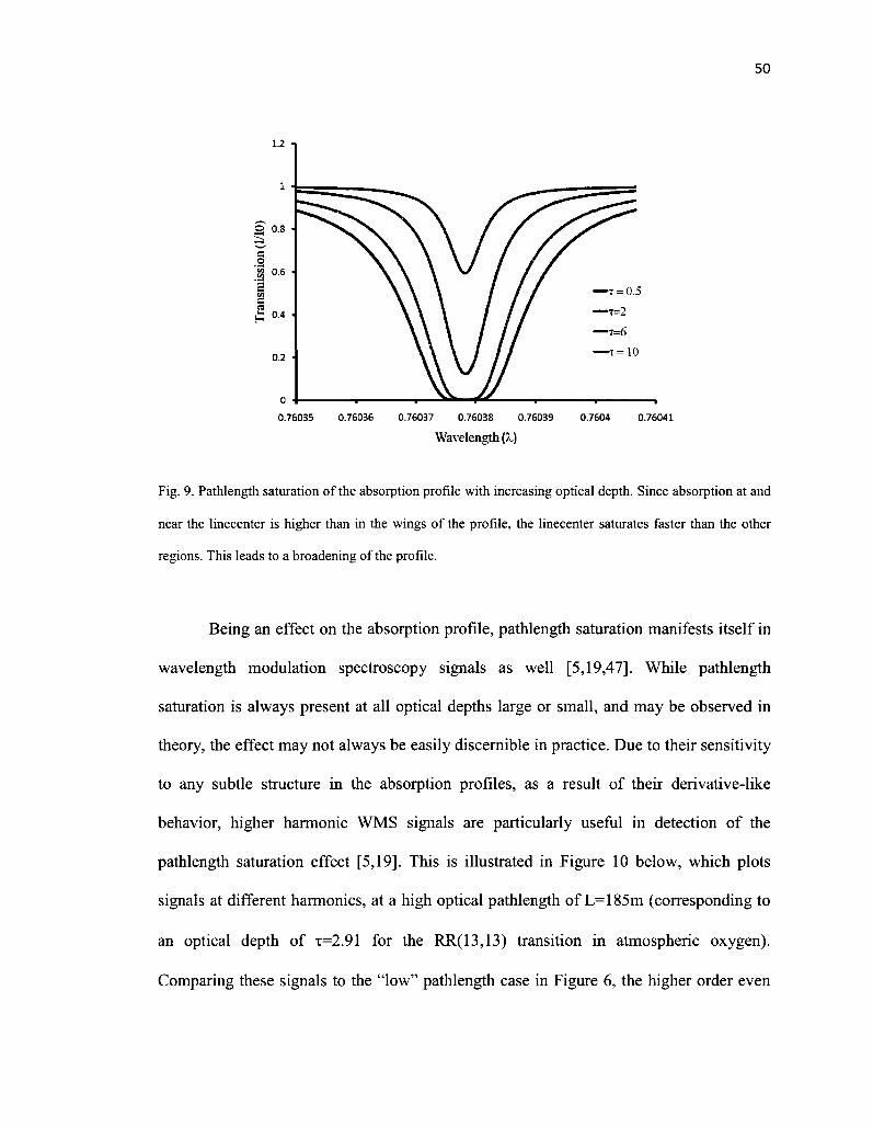
50

H

0.76035 0.76036 0.76037 0.76038 0.76039 0.7604 0.76041

Wavelength (?J

Fig. 9. Pathlength saturation of the absorption profile with increasing optical depth. Since absorption at and

near the linecenter is higher than in the wings of the profile, the linecenter saturates faster than the other

regions. This leads to a broadening of the profile.

Being an effect on the absorption profile, pathlength saturation manifests itself in

wavelength modulation spectroscopy signals as well [5,19,47]. While pathlength

saturation is always present at all optical depths large or small, and may be observed in

theory, the effect may not always be easily discernible in practice. Due to their sensitivity

to any subtle structure in the absorption profiles, as a result of their derivative-like

behavior, higher harmonic WMS signals are particularly useful in detection of the

pathlength saturation effect [5,19]. This is illustrated in Figure 10 below, which plots

signals at different harmonics, at a high optical pathlength of L= 185m (corresponding to

an optical depth of T=2.91 for the RR(13,13) transition in atmospheric oxygen).

Comparing these signals to the "low" pathlength case in Figure 6, the higher order even

51

harmonics (N=6 and N=8) show a clear suppression of the peak at linecenter at the higher

pathlengths. Furthermore, this effect is not easily visibly at direct absorption or the lower

harmonic signals. In a similar manner, the peaks around the linecenter of higher order

odd harmonics (N=7) are also suppressed.

A large modulation index, however, has an inverse effect on the detection of

pathlength saturation. In general, a higher modulation index results in a broadening of the

WMS signals, which tends to mask the spectral resolution. For example, while a higher

detection harmonic order offers the possibility of resolving congested spectra [3,7], an

increased value of the modulation index m and the resultant modulation broadening

reduces the ability to resolve adjacent lines. Likewise, a higher modulation index results

in the loss of the peak suppression that higher harmonics show at high optical

pathlengths. This is illustrated in Figure 11, which compares the detection signals at

N=6,7 and 8 for two different modulation indices at the same pathlength of L= 185m. The

peak suppression that is present at N=6 when m=2.5 is no longer visible when the

modulation index is increased to m=3.12. Likewise, the peaks around and at linecenter

for N=7 and 8 are no longer as suppressed as at the lower modulation index. There is

therefore an optimal range of modulation indices in which the pathlength saturation effect

is most evident [5,19].

Chapter 3 will present experimental results, with theoretical model comparisons,

verifying the aforementioned behaviors of wavelength modulation spectroscopy signals.

We also show that the structure of WMS signals, along with pathlength saturation effects,

provides a sensitive diagnostic for structure of lineshape functions.

52

N=0 N=2 1 -

0.995 :

—. 0.99 •) d

j j 0.985 -: > •

£ o.9S -

- 0.975 J

0.97 -

0.965 4

0.760365 0.76037 0.760375 0.7603S

Wavelength (A)

0.760385 0.76039

Inte

nsity

(a, u

.)

1.0E+0

9.0E-1 -

8.0E-1 -

7.0E-1 -

6.0E-1

S.OE-l

4.0E-1

3.0E-1

2.0E-1

l.OE-3

O.OE+O

0.76035 0.76036 0.76037 0.76038 0.76039

Wavelength (A)

0.7604 0.76041

N=5 N=6

O.OE+O

0.76035 >76037 0.76038 0.76039 0,7604 0,76041

Wavelength (/,)

0.76035 0.76036 0.76037 0.76038 0.76039 0.7604 0.76041

Wavelength (?.)

N=7 N=8

176036 0.76037 0.76038 0.76039 0.7604 0.76041

Wavelength (A)

1.4E-2

1.2E-2

_ l.OE-2 I

3. 8.0E-3

| -- 4.0E-3

2.0E-3 J

0.76035 0.76036 0.76037 0.76038 0.76039 0.7604 0.76041

Wavelength (A)

Fig. 10. Pathlength saturation effects at higher harmonic wavelength modulation spectroscopy signals, at

high optical pathlength of L=185m. The peaks at and around linecenter are suppressed at the higher

harmonics (compare to Figure 6), an effect not present at direct absorption or lower detection harmonic

orders. The signals are calculated for a modulation index of m=2.5.

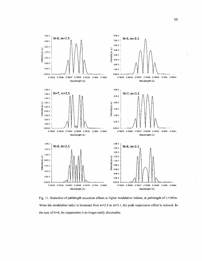
53

7.0E-2

60E-2

* 5.0E-2 -

i £ • 4.0E-2

£ 3.0E-2

2.0E-2

1.0E-2

O.OE»0 -

N=6, m=3.1

A 11 0.76036 0.76037 0.76038 0.76039 0.7604 0.76041

Wavelength (X)

0.76035 0.76036 0.76037 0.76038 0.76039 0.7604 0.76041

Wavelength {>.)

O.OE+O

0,76035 0.76036 0.76037 0.76038 0.76039 0.7604 0,76041

Wavelength (X)

N=7, m=3.1

0.76035 0.76036 0.76037 0.76038 0.76039 0.7604 0.76041

Wavelength (?.}

1.2E-2

l.OE-2

2. 8.0E-3

f -4.0E-3

2.0E-3

0.0E+0

N=8, m=2.5

0.76O36 0.76037 0.76038 0.76039 0.7604 0.76041

Wavelength (X)

0.76035 0.76036 0.76037 0.76038 0.76039 0.7604 0.76041

Wavelength (X.)

Fig. 11. Reduction of pathlength saturation effects at higher modulation indices, at pathlength of L= 185m.

When the modulation index is increased from m=2.5 to m=3.1, the peak suppression effect is reduced. In

the case of N=6, the suppression is no longer easily discernable.

54

2.4 LINESHAPE PROFILES

In any absorption experiment, the frequency absorbed or emitted by a particular

transition in the atom or molecule is not a single value, i.e. a delta function. Rather, the

absorption or emission profile is broadened by some process occurring during the

interaction of light with matter. For example, at the most fundamental level (the atomic

level), the energy levels of stationary states are broadened due to the Heisenberg

Uncertainty Principle [29]. Therefore, the frequency spectrum of absorption or emission

will be broadened as well, taking on a Lorentzian shape. We used this basic fact when

calculating the Einstein A21 coefficients, which are an important component of the

absorption cross section of transitions. In fact, A21 values are experimentally determined

by measuring linewidths and radiative lifetimes of transitions between the stationary

states of interest [48].

Heisenberg (also called "lifetime" or "natural") broadening, however, is much

weaker than the broadening that arises from the dynamics of the atoms and molecules.

There are various lineshape profiles that address the different broadening mechanisms,

such as the Lorentzian, Gaussian, Voigt, Galatry [49], Rautian-SobePman [50], speed-

dependent Berman [51], and many more. The Gaussian and Lorentzian profiles are

fundamental and form the basis for the other broadening descriptions, and are thus

described in detail in this section. We also derive the Voigt profile, which is a

combination of the Doppler broadened (Gaussian) and collision broadened (Lorentzian)

profiles.

55

2.4.1 Doppler Broadening

The Doppler Effect is the frequency shift that occurs as a source of waves moves

towards or away from the observer. This relative motion with respect to the observation

reference frame leads to a broadening of the lineshape profile. Radiation from emitters

moving towards the observer is shifted towards the blue spectrum, while that from atoms

or molecules moving away from the observer is red shifted. Doppler broadening is the

dominant broadening mechanism at low pressures, where mean-free-paths are large (and

time between collisions is large).

The Doppler shifted observed frequency for an atom or molecule emitting at

frequency vo moving towards an observer (e.g. a photodetector) at velocity u, is given by:

'l + - l (60)

where c is the speed of light (Note that this is the non-relativistic Doppler effect). Every

emitter, in a gaseous medium for example, contributes this Doppler shifted frequency

component to the total emission. Furthermore, the contribution scales accordingly with

the distribution of velocities of the emitting atoms and molecules. Thus, if p(u)du is the

probability of finding a molecule with velocity between u and u+du, then the probability,

g(v), of observing a frequency between vand v+dv along the line of sight is:

du g(y)dv = p(u)—dv (61)

dv

Substituting (60) into (61), we obtain:

( ( S\ r v

(62)

g(y)=—p

Vvo J J

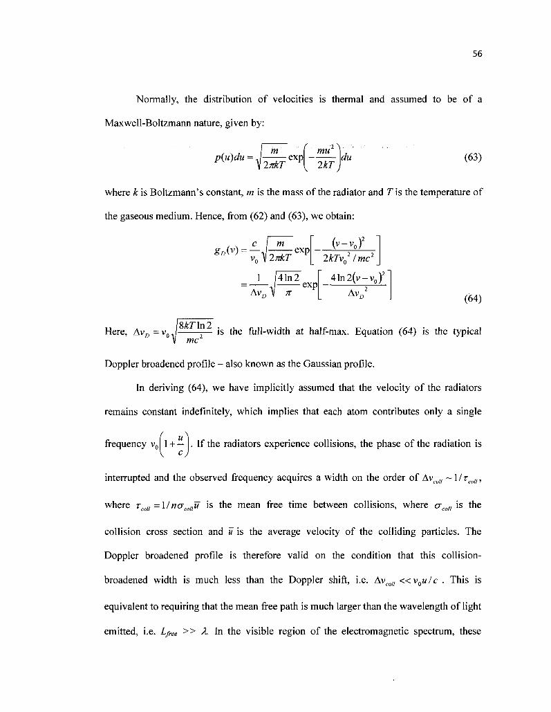
56

Normally, the distribution of velocities is thermal and assumed to be of a

Maxwell-Boltzmann nature, given by:

p(u)du = m 2nkT

exp ' mu2

2kT \du (63)

where k is Boltzmann's constant, m is the mass of the radiator and Tis the temperature of

the gaseous medium. Hence, from (62) and (63), we obtain:

(v-v0)2

gD(v) = ~ m v0 V 2nkT

exp

1 41n2

AvD V n •exp|

2kTv021 mc2

41n2(v-v0)2

Avn2

(64)

Here, AvD=v0J — is the full-width at half-max. Equation (64) is the typical

V mc

Doppler broadened profile - also known as the Gaussian profile.

In deriving (64), we have implicitly assumed that the velocity of the radiators

remains constant indefinitely, which implies that each atom contributes only a single

frequency vc v cj

. If the radiators experience collisions, the phase of the radiation is

interrupted and the observed frequency acquires a width on the order of Avcoll ~MTCOII,

where rcoll =\lnacollu is the mean free time between collisions, where crcoll is the

collision cross section and u is the average velocity of the colliding particles. The

Doppler broadened profile is therefore valid on the condition that this collision-

broadened width is much less than the Doppler shift, i.e. Avcoll «v0u/c . This is

equivalent to requiring that the mean free path is much larger than the wavelength of light

emitted, i.e. Lfree » A. In the visible region of the electromagnetic spectrum, these

57

conditions hold only at low densities or low pressures. If the motion of the radiators is

restricted by collisions, such as with other particles or the walls of the container, there are

other elements that must be considered towards the broadening of the profile.

2.4.2 Collision Broadening

In collision broadening, the waves emitted by radiators are assumed to undergo a

random series of dephasings, as a result of elastic collisions with other molecules. The

broadening that results from this process is generally described by the Lorentzian

lineshape function. We will derive the collision broadening profile under some first order

assumptions, commonly known as the impact approximation [52]. First, the relative

motions of the colliding particles are assumed to be semi-classical. Second, we assume

that the collision time is much smaller than the mean time between collisions, which are

therefore assumed to occur instantaneously.

Under these assumptions, let us consider what happens when a radiating particle

collides with another particle. During the collision, the electric field of the perturbing

particle affects the internal energy level structure of the emitting atom or molecule. As a

result of the random nature of the collisions, the phase of the electric field emitted by the

radiator is randomized as well [52-53]. The broadening of the transition is thus the result

of these collisions. We write the emitted electromagnetic wave as:

E(t) = exp[ia)0t + ij](tj\ (65)

where rj(t) is the random phase shift caused by the collisions, and coo is the unperturbed

frequency of the emitting particle. The power spectrum of the field can then be

determined from a Fourier analysis. The Fourier transform of the electric field is:

58

J (a) = JE(t)e~'°"dt = jexp[/(&>0 - co)t + irj(t)}it 0 0

with the power spectrum given by [52]:

I(a>) = \j(a>)\2

0 0 0 0

— 0 0 — 0 0

OO CO

(66)

Since the phase rj is a random function, the second integral represents an average

[52]. We will determine this average for a simple case - assuming that only three possible

phase changes can occur upon collision, r/a, rib and r/c. This approach can, however, be

extended in a straightforward manner to include any number of possible phase changes,

including the continuous limit. We also assume that each phase change has a collision

cross section cr„ and the total cross section is aj = cra+(Jb+crc. Thus, the probability of n

collisions of type a, m of type b and / of type c, occurring in time t, is given by the

Poisson distribution [52]:

r_ v \aT J

f _ A V A

v°V j

1

KaT J

(67) m\n\l\\T t

where ris the mean time between collisions. Under these assumptions, the average of the

exponential term in (66) can be shown to be [52]:

AnO+O-niO}^ = expl J_^y*. + ^ + ay»c ]1 (68)

Substituting equation (68) into (66), we obtain for the intensity, which is a real

quantity:

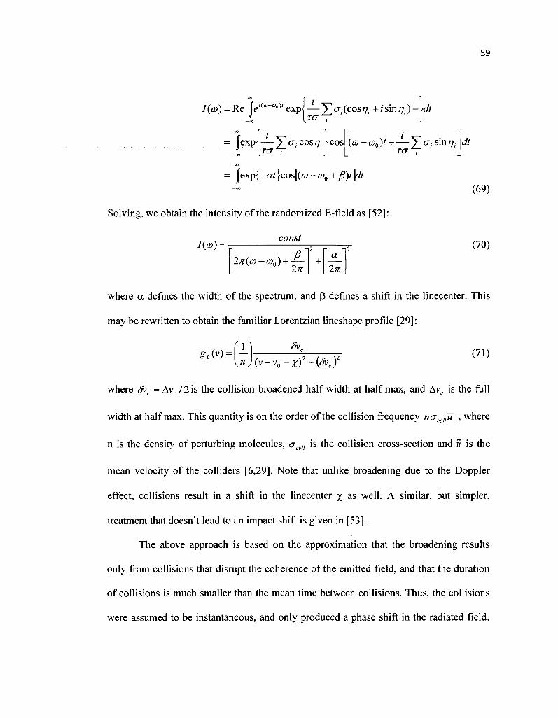
59

I(a>) = Re je*"-"0* expj — £ a, (cosr\t + isin 7,) - \dt

= f e x Pi—X°" ' c o s ^r c o s (»-*><>)'+—Z°"'sin77'

= jexp{- ctf }cos[(<y -a>0+ f3)t\lt

Solving, we obtain the intensity of the randomized E-field as [52]:

const

dt

I(co) = -

2n(a>-co0) + 2n + a

~2n

(69)

(70)

where a defines the width of the spectrum, and p defines a shift in the linecenter. This

may be rewritten to obtain the familiar Lorentzian lineshape profile [29]:

gL(y) = \n )

Sv„

(v-v0-z)2+{Svcf (71)

where Svc = Avc /2is the collision broadened half width at half max, and Avc is the full

width at half max. This quantity is on the order of the collision frequency nacollu , where

n is the density of perturbing molecules, acoll is the collision cross-section and u is the

mean velocity of the colliders [6,29]. Note that unlike broadening due to the Doppler

effect, collisions result in a shift in the linecenter 1 as well. A similar, but simpler,

treatment that doesn't lead to an impact shift is given in [53].

The above approach is based on the approximation that the broadening results

only from collisions that disrupt the coherence of the emitted field, and that the duration

of collisions is much smaller than the mean time between collisions. Thus, the collisions

were assumed to be instantaneous, and only produced a phase shift in the radiated field.

60

As a result, the collision broadened profile is a good approximation when modeling

instances where the pressure is very high (thus meeting our assumptions). Any physical

system however involves a combination of both Doppler and Collision broadening, which

is discussed in the next section.

2.4.3 Simultaneous Doppler and Collision Broadening: Voigt Profile

There are many approaches to treating the lineshape profile that arises from

simultaneous Gaussian and Lorentzian broadening. In one particular approach, we

assume that broadening due to the Doppler Effect is statistically independent from the

broadening due to interaction with perturbing particles (collisions), because the two

profiles arise from different physical mechanisms. Under this assumption, we can derive

the Voigt lineshape function, which we use when modeling the experimental results in

this dissertation.

As shown, the broadening due to the translational motion of radiating atoms and

molecules under Maxwell-Boltzmann thermal statistics leads to the Gaussian profile.

Likewise, collisions with surrounding particles can be described by a Lorentzian

lineshape function. That is:

gD(z) = rx\"

2

\nj

1

AvD ^exp

( \

VAlW (72)

'^hf%j

61

Avr where Avn = , V41n2

is the normalized Doppler linewidth, and z = v-v0. Under the

assumption of statistical independence between the two probability density functions, the

combined profile can be easily determined from a convolution of the two lineshape

functions:

CO

gv(z) = SD (*) * gL (z) = \gD (z')gL(z-z')dz'

f _, V •gy(y) =

\7TJ ntSv exp

D -co Av Dj

Sv„

(z-z')2+(svcy -dz'

(74)

Making the substitution of variables y = z'/AvD and dy = dz'/AvD , equation (74)

becomes:

gy(z) = 1

*™J J_ exp tz l

f \ z rAT^ K ^ j

y

-dy (75)

+ 1

We simplify this expression by defining the normalized frequency x = v-v„ <Sv„ <5v„

and

Sv the parameter b = c , which leads to the well known Voigt lineshape profile:

Av

gv(*): ( 1 A 1 ™

v ^ 3 / 2 ; - -exp ( - / ) -dy (76)

It can be seen that as the collision frequency, and therefore, Svc , goes to zero, the

Voigt function parameter, b, tends to zero as well. Hence in the limit of low density and

pressure, b«l and equation (76) reduces to the Gaussian profile. On the other hand, as

b»l, the profile takes on a Lorentzian shape, with the width determined mostly by the

62

phase changes occurring during collisions. Hence, b is a measure of the contributions of

Doppler and collision broadening components to the total profile.

The above profile was derived under the assumption that the collision and

Doppler broadening are statistically independent; effectively implying that dvc is

independent of velocity. This assumption holds only when the mean free path between

collisions is much larger than the wavelength emitted by the radiators. Thus, while the

Voigt profile is able to model most experiments with sufficient accuracy, this accuracy

depends on the absorbing species and the environment.

In general, however, the role of collisions in broadening is quite complex, as

collisions can perturb the translational motion of the radiating particles, as well as affect

the internal energy states. The exact lineshape function of a particular molecular

transition is multifaceted, and the dynamics of molecular collisions result in effects not

described by the simple and commonly-used impact approximation. For example,

collisions resulting in a constraint on the translational degree of freedom of an absorber

or emitter due to neighboring scattering particles result in a line narrowing, first predicted

by Dicke [54] and subsequently shown by him and others [55-56]. Furthermore, one can

expect the broadening due to collisions with species identical to the radiator ("self-

broadening") to be different than that due to collisions in a mixture of gases, such as air

for instance (often referred to as "air broadening").

For the experimental work described in this dissertation, which was done at

atmospheric temperatures and pressures, the Voigt profile was adequate under the

precision and resolution available. Higher order lineshape profiles would normally be

required to describe collisional narrowing, but these effects are only significant at higher

63

pressure under the resolutions available. Furthermore, in the environment of the

experiment, the b parameter was large enough such that the Lorentzian and Voigt

functions gave very similar absorption profiles. The resulting harmonic signals from

these two profiles are compared with experimentally obtained WMS signals, presented in

the Chapter 3. We show that higher harmonic detection allows us to determine with

greater confidence which profile gives more accurate models of an experiment, than

lower detection orders and direct absorption, when the profiles have nearly identical

shapes.

64

CHAPTER III. SIMULTANEOUS HIGHER HARMONIC WMS

MEASUREMENTS OF ATMOSPHERIC OXYGEN

In this chapter, we present experimental results with theoretical comparisons for

wavelength modulation spectroscopy of the A-band of atmospheric oxygen, utilizing

simultaneous multiple harmonic detection. The experimental apparatus for phase

sensitive detection is discussed, and we detail the motivation behind, and development of,

a simultaneous higher harmonic detection system. The system was designed and

implemented on a National Instruments Labview platform, and the output was verified

against that of a Stanford Research Systems Lock-In Amplifier that has been previously

used extensively by the same research group. The absorption signals at various harmonics

for different transitions in the Oxygen A-band were obtained and compared with

theoretical models.

The theoretical models were developed with two profiles: one utilizing a

Lorentzian lineshape function and another utilizing the Voigt lineshape function. Since

the experiments were performed at atmospheric pressure and temperature, the collision

linewidths were approximately three times greater than the Doppler broadening. As a

result, the b parameters of the Voigt function were relatively large and the two models

produced nearly identical signals at direct absorption, making them difficult to

distinguish at the resolutions available. Wavelength modulation spectroscopy is,

however, shown to be a useful tool for distinguishing between the two profiles,

particularly at higher harmonics. This has especially important applications for the

65

investigation of line structure and molecular dynamics, since that information is

contained in the finer features of the lineshape profile.

We also demonstrate the utility of wavelength modulation spectroscopy in the

resolution of weak spectra. From experimental results and modeling, we find that higher

harmonic signals result in a greater amplification of the weaker transitions compared to

the relatively stronger lines. It must be noted that the "strong" lines referred to here are

already much weaker (by at least six orders of magnitude) than what would normally be

considered a "strong" transition in conventional direct absorption spectroscopy. The

"weak" transitions are a further three to five orders of magnitude weaker. Therefore,

transitions that would not normally be visible at direct absorption or lower harmonic

orders under a given experimental resolution become visible at higher harmonics. This

has useful applications, for example, in the measurement and study of isotopes.

3.1 EXPERIMENTAL PROCEDURE

3.1.1 Sequential Higher Harmonic Detection

The experimental setup used to perform wavelength modulation spectroscopy is

illustrated in Figure 12. The apparatus consists of a tunable diode laser, temperature

controller, function generator and ramp that feed into a laser driver and a photodetector

and lock-in amplifier combination on the receiving end. While most common edge

emitting lasers are tunable over several hundred wavenumbers, we utilize a VCSEL,

which is easily tuned by adjusting the injection current and has a sufficient tunability

range for the lines of interest. The temperature controller and DC current from the laser

driver are first used to set the starting frequency of the laser. In our experiments

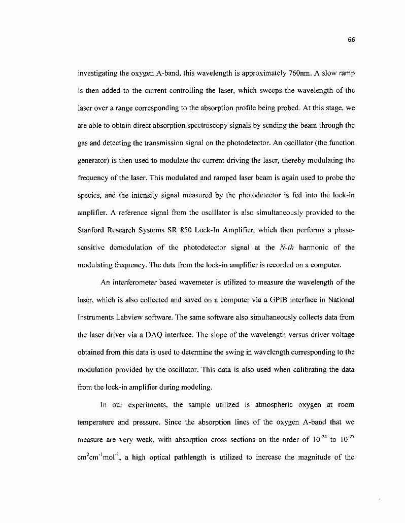
66

investigating the oxygen A-band, this wavelength is approximately 760nm. A slow ramp

is then added to the current controlling the laser, which sweeps the wavelength of the

laser over a range corresponding to the absorption profile being probed. At this stage, we

are able to obtain direct absorption spectroscopy signals by sending the beam through the

gas and detecting the transmission signal on the photodetector. An oscillator (the function

generator) is then used to modulate the current driving the laser, thereby modulating the

frequency of the laser. This modulated and ramped laser beam is again used to probe the

species, and the intensity signal measured by the photodetector is fed into the lock-in

amplifier. A reference signal from the oscillator is also simultaneously provided to the

Stanford Research Systems SR 850 Lock-In Amplifier, which then performs a phase-

sensitive demodulation of the photodetector signal at the N-th harmonic of the

modulating frequency. The data from the lock-in amplifier is recorded on a computer.

An interferometer based wavemeter is utilized to measure the wavelength of the

laser, which is also collected and saved on a computer via a GPIB interface in National

Instruments Labview software. The same software also simultaneously collects data from

the laser driver via a DAQ interface. The slope of the wavelength versus driver voltage

obtained from this data is used to determine the swing in wavelength corresponding to the

modulation provided by the oscillator. This data is also used when calibrating the data

from the lock-in amplifier during modeling.

In our experiments, the sample utilized is atmospheric oxygen at room

temperature and pressure. Since the absorption lines of the oxygen A-band that we

measure are very weak, with absorption cross sections on the order of 10~24 to 10"27

cm2cm"1mor1, a high optical pathlength is utilized to increase the magnitude of the

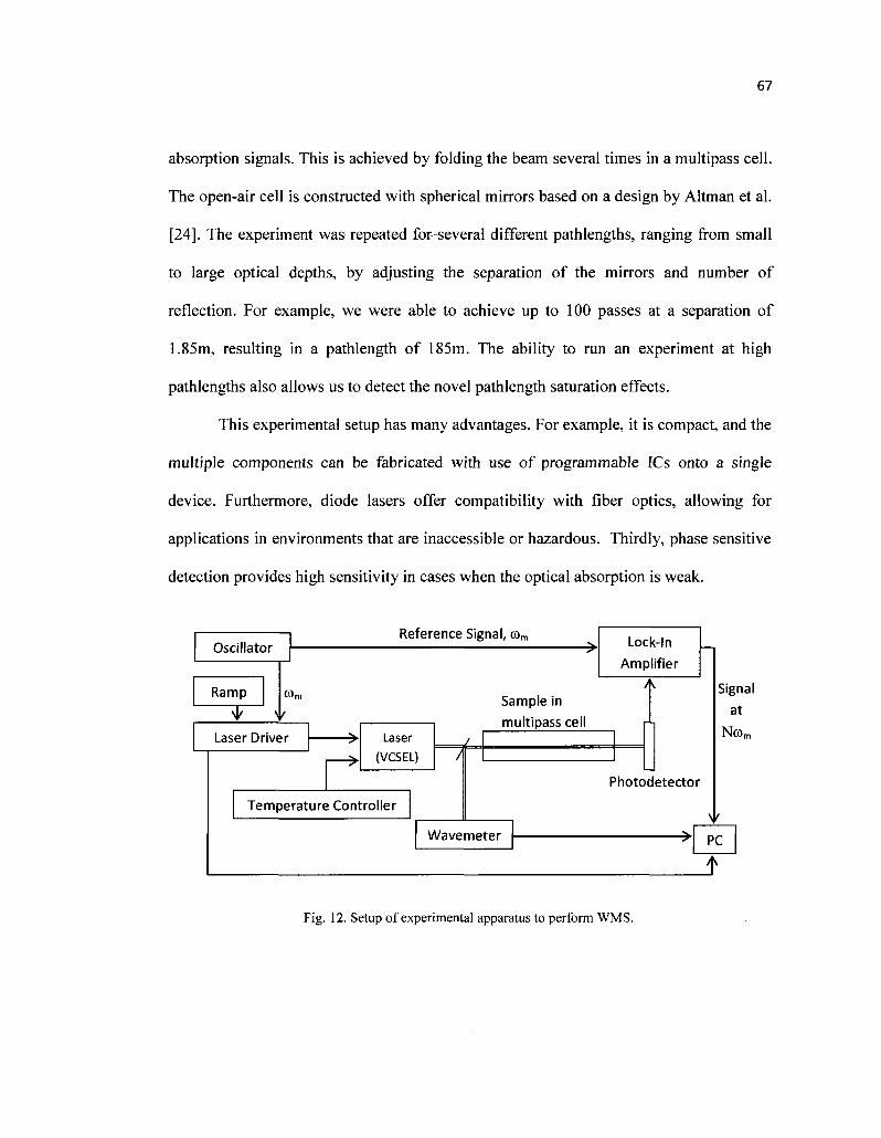
67

absorption signals. This is achieved by folding the beam several times in a multipass cell.

The open-air cell is constructed with spherical mirrors based on a design by Altman et al.

[24]. The experiment was repeated for several different pathlengths, ranging from small

to large optical depths, by adjusting the separation of the mirrors and number of

reflection. For example, we were able to achieve up to 100 passes at a separation of

1.85m, resulting in a pathlength of 185m. The ability to run an experiment at high

pathlengths also allows us to detect the novel pathlength saturation effects.

This experimental setup has many advantages. For example, it is compact, and the

multiple components can be fabricated with use of programmable ICs onto a single

device. Furthermore, diode lasers offer compatibility with fiber optics, allowing for

applications in environments that are inaccessible or hazardous. Thirdly, phase sensitive

detection provides high sensitivity in cases when the optical absorption is weak.

Oscillator

Ramp co„

Laser Driver

Reference Signal, co„

Laser

(VCSEL)

Temperature Controller

Lock-In

Amplifier

•71

Sample in

multipass cell

Photodetector

Wavemeter

Signal

at

Ncom

PC

T Fig. 12. Setup of experimental apparatus to perform WMS.

68

3.1.2 Simultaneous Higher Harmonic Detection

In the above setup, absorption signals at the different harmonics are collected

sequentially - that is, one first collects data at N = 1, then proceeds to N = 2, and so on.

This makes the experiment susceptible to any changes in the properties of the gas being

probed, such as temperature, pressure, density, etc. that might occur during the

acquisition of data at different harmonics. Hence, the parameters of the gas when the N=l

harmonic signal is detected, may be different than that when N=2 or any other harmonics

are measured - with this change occurring on the order of the ramp time. Out in the field

in an open environment, sequential measurements become even more vulnerable to a

changing environment; much more so than in the laboratory setup above, where there is

always an attempt (although never completely successful) to control such variations. In

addition, one may be constrained by time limits. The compilation of data at N harmonics

sequentially necessitates at least N times the time required to probe one harmonic.

Therefore, there is a need to develop a simultaneous higher harmonic detection

system, capable of obtaining signals at multiple harmonics in a single sweep. The

experimental setup in §3.1.1 was modified to allow for such a process. The new setup

utilized for simultaneous multiple higher harmonic detection is illustrated in Figure 13.

The apparatus used is identical to that for sequential detection, with one key

modification: instead of utilizing the SR 850 Lock-In Amplifier, we perform phase

sensitive detection virtually, in a program implemented in Labview. The absorption

signal from the photodetector and the reference signal from the oscillator are collected

with an NI-4474 DAQ Data Acquisition system. Because the input impedance of this

DAQ card is fairly low (approximately 200kQ), a buffer amplifier is placed between the

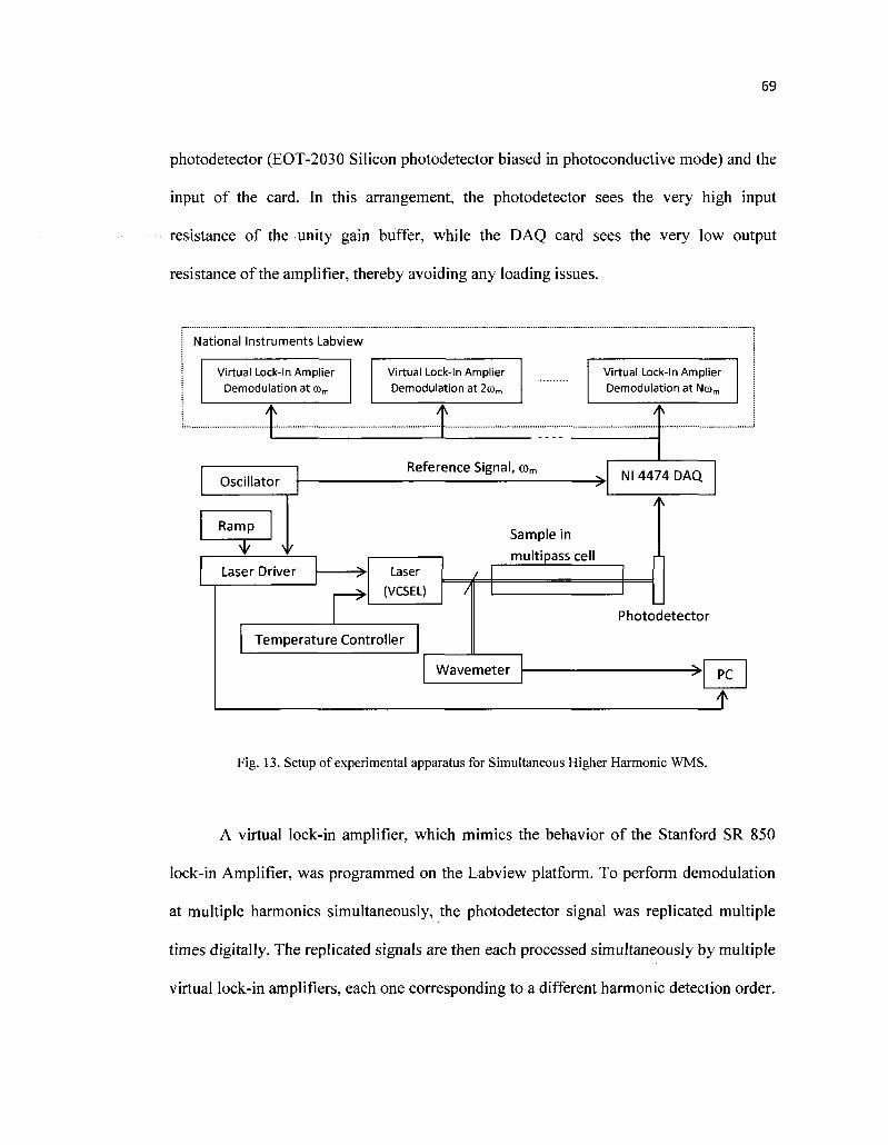
69

photodetector (EOT-2030 Silicon photodetector biased in photoconductive mode) and the

input of the card. In this arrangement, the photodetector sees the very high input

resistance of the unity gain buffer, while the DAQ card sees the very low output

resistance of the amplifier, thereby avoiding any loading issues.

; National Instruments Labview

Virtual Lock-In Amplier Demodulation at » m

/ V

Virtual Lock-In Amplier Demodulation at 2com

A

Virtual Lock-In Amplier Demodulation at Ncom

/\

Oscillator

Ramp

* \

Reference Signal, com

s Nl 4474 DAQ

M

Sample in t

Laser Driver >1 s -^

Laser

(VCSEL)

Temperature Controller

/ /

Photodetector

Wavemeter >4 S PC

t

Fig. 13. Setup of experimental apparatus for Simultaneous Higher Harmonic WMS.

A virtual lock-in amplifier, which mimics the behavior of the Stanford SR 850

lock-in Amplifier, was programmed on the Labview platform. To perform demodulation

at multiple harmonics simultaneously, the photodetector signal was replicated multiple

times digitally. The replicated signals are then each processed simultaneously by multiple

virtual lock-in amplifiers, each one corresponding to a different harmonic detection order.

70

The algorithm utilized to perform each lock-in amplifier operation is described in the

block diagram, shown in Figure 14. A phase-lock-loop algorithm processes the signal

collected on the reference channel, and determines the frequency of the reference signal.

It then generates sine and cosine signals at the N-th harmonic of that frequency - both of

which are in phase with the reference signal. The sine and cosine signals are then

multiplied with the photodetector signal. Since this signal can be decomposed into a

Fourier series, the resulting signal from the multiplication has two components around

each harmonic: the frequency of the first is the difference between the Na>m Fourier

components of the photodetector signal and the phase lock loop signal, e.g. cos(N-

l+<j>i)a)mt and sin(N-l+<|)i)comt; while the second is at the sum, e.g. cos(N+l+<j)i)o)mt and

sin(N+l+(j)i)comt. Here, <j>N is the phase difference between the N-th component of the

photodetector signal and the reference signal. Thus, the result of the multiplication will

always have a DC component corresponding to the N-th Fourier component of the

photodetector signal. A low pass filter can then be used to isolate these DC components,

labeled X and Y corresponding to the cosinusoidal and sinusoidal Fourier components of

the signal, respectively. From these, we can readily determine the magnitude signal, RN,

and the phase, <J)N.

71

Photodetector Signal

RjCOSfcOmt+((»,)

+ R2cos(2(omt+(t)2)

+...+ RNcos(Ncomt+(|)N) +.,

Reference Signal, ram

JU

.0 RiCOSfN+l+ iJCOmt

+ RiCOs(N-l- <t>i)comt

+...+ RNcos(2N+ <t>N)comt

+ RNcos((|)N) +.... Low Pass

Filter

cos(N<amt)

Phase-Lock Loop

sin(Ncomt)

T XN = RNcos(<|>N)

RN =

(XN +YN ) 0N=tan"1(YN/XN)

YN = RNsin(<t>N)

• &

Low Pass

Filter

RiSinfN+l+^Joimt

+ RiSinfN-1- <t>i)comt+...+RNsin(2N+ <|>N)comt

+ RNsin(<()N) +....

Fig. 14. Block diagram algorithm of phase-sensitive detection performed by a lock-in amplifier.

The simultaneous multiple harmonic lock-in amplifier program that was

implemented in Labview is given in Appendix A. The user-interface is composed of

controls allowing the operator to change the LIA parameters. In particular, one can adjust

the collection time, number of samples per second collected, and the filter algorithm and

time constant (i.e. bandwidth). This last quantity is very important, as it acts as a noise

filter. However, since the filter performs an averaging, the bandwidth must be kept small

enough so as not to average out the harmonic signals. The output of the program is

displayed on real time charts of each harmonic, along with the X, Y, R and <j) values, as

shown in Figure 15, as well as saved to a spreadsheet file. The work done in this

dissertation measured the magnitudes of the harmonic signals (i.e. R-signals).

Fig. 15. Interface of Simultaneous Harmonic Detection program in Labview. Shown are the signals for

N=4,5,6 and 7, obtained simultaneously in one sweep of the laser across the absorption profile.

The quality of this virtual lock-in amplifier was judged by comparing data

obtained through it to that from the Stanford SR 850 system. One such set of comparisons

is provided in Figure 16. The plots shown are signals at different harmonics between N=l

through 8, for an experiment probing the RR(13,13) line of the atmospheric oxygen A-

band. According to HITRAN [39], the linecenter of this transition is located at

13151.34866 cm"1, corresponding to wavelength of 760.37829 nm. The laser was

therefore swept from 760.30nm to 760.40nm. The experiment was run at an absorption

pathlength of L=68m, and modulation index m=4.1. The quantity, A, is the mean absolute

73

percent difference with respect to the SR 850 data, across the profile. The harmonic data

for the SR 850 system was collected sequentially, each sweep lasting approximately 45

seconds. All harmonics collected by the Labview system were obtained simultaneously,

in a single sweep. While we show just one set of the data here, the experiment was

repeated several times with the same results. Also, while the figure shows only N=l to 3

and 6 to 8, data was collected for all harmonics (including N=4 and 5).

We find that the signals of the Labview designed LIA are within approximately

4.5% of the Stanford LIA system. This cumulative difference is even smaller at the lower

harmonics; with the greater discrepancy at higher harmonics being due to the larger

amount of noise, relative to the signal, present there. This is because the signals become

progressively weaker as the detection order is increased. As a result, the contribution of

noise is greater, which distorts the total signal and therefore the average discrepancy, as

can be seen in Figures 16(e) and 16(f). The positive and negative limits on the percentage

differences are determined from the standard deviation of the discrepancy across the

absorption profile.

74

4.5E-1

4.0E-1

k 3.5E-1

; 3.0E-1

2.5E-1

2.0E-1

, 1.5E-1

1.0E-1

5.0E-2

O.OE+0

—SR 850 LIA —Labview Virtual LIA

(a) N = 1, A = 0.21 ±0.011%

760.37829

Wavelength |nm)

6.0E-2

5.0E-2

! " B 3.0E-2

1.0E-2

0.0E+O

(c) N = 3, A = 0.77±0.03%

1.4E-1 r

1.2E-1 •

> 1.0E-1

| 8.0E-2 £ .E 6.0E-2

2.0E-2

0OE+0

(b)N = 2

A = 0.36±0.018%

760.37829 Wavelength (nm)

1.0E-2

> 8.0E-3

| 6.0E-3

I*** 2.0E-3

0.0E+0

(d) N = 6, A = 2.33±0.13%

760.37829 Wavelength (nm)

760.37829

Wavelength (nm)

6.0E-3

5.0E-3

> j * t.OE-3

c B 3.0E-3 c

"ro §> 2 f " in

1.0E-3

O.OE'O

(e) N = 7, A = 3.61±0.18%

760.37829

Wavelength (nm)

3.5E-3

3.0E-3

S . 2.6E-3

£ 2.0E-3

3 1.5E-3 CO

c 9> 1.0E-3

W

5.0E-4

0 0E+0

(f) N = 8, A = 4.53±0.22%

760.37829

Wavelength (nm)

Fig. 16. Comparison of harmonic signals obtained with a Stanford SR 850 (Blue) lock-in amplifier, against

those obtained with a virtual simultaneous multiple harmonics lock-in amplifier on Labview. The quantity

A is a measure of the cumulative percentage difference (absolute) between the two sets, with respect to the

SR 850 system.

75

3.1.3 Modeling the Experimental Data

All the experiments presented in this dissertation are modeled using Wilson's

method, i.e. equation (47), with the appropriate form of the lineshape function. The

absorption parameters, such as linecenter, collision linewidth and integrated absorption

cross-sections, are obtained from the HITRAN 2008 database [39]. The Doppler

linewidth is estimated from the room temperature of approximately 296K. These values,

however, differ from the actual values of the experimental parameters, and are therefore

used as a starting point (For example, the HITRAN linewidths for the A-band have been

known to be off by up to 30% [20]). The parameters are therefore adjusted to obtain the

best match between experiment and theory.

The best fits between theoretical and experimental data are obtained under highly

stringent constraints: for a given set of data (direct absorption and N=l to 8),

corresponding to a particular modulation index and pathlength, we sought the best match

between experiment and theory at the highest harmonic obtained, i.e. N=8. This requires

matching at least the 2N+1 turning points, i.e. 17 zero-crossing and maxima, at N=8.

Furthermore, since the experiment did not measure the optical intensity, we normalized

the data by setting equal the line center peaks of the experimental and theoretical data.

All other experimental data sets were then compared to theoretical models obtained from

these parameters, with no other adjustments made, except changing the harmonic order

N, the modulation m and the pathlength L, as appropriate, in the model.

In this manner, we use the structure of WMS signals as a self-consistent check in

any conclusions drawn. With the forced normalization (between theory and experiment)

of the one point corresponding to the line center at N = 8, each set of experimental data

76

for a fixed path length and fixed modulation index must fall into place at at least 2N+1

turning points and zero crossings, summed over N=0,l,2,...8. This means that each fit

requires at least i 2_,(2N +1) >-1 = 80 experimentally independent points to match with

U=o J

the modeled results, per transition. Of course, the quality of the matches was still judged

over the entire absorption signal, and not only at these salient points. The modulation

index, m, was measured each time a set of experimental data was obtained. The

linewidths and cross-sections thus obtained from one set of results were then used for all

the other results, for all modulation indices and all pathlengths, each time only the one

normalization at the line center of N = 8 signal being applied.

We probed the RR(13,13) and RQ(11,12) transitions of 0-16, and the RQ(11,12)

and RR(12,12) transitions of 0-18. These latter isotopic transitions are two orders of

magnitude weaker than the former, owing to the lower concentration of the isotope. The

relevant modeling parameters from HITRAN for these transitions at 293K and 1 atm

pressure, which were used in a Matlab program (provided in Appendix B), are given in

Table 2 below. Molecular Oxygen A-band Parameters

Transition Species Wavelength Absorption Cross-Section Atmospheric Concentration (ixm) (cm2 cm'1 mol') (at 293K; cm"3)

RR(13,13) l b 0 2 0.76037829 5.64 xlO"24 5.14 xlO1 8

RQ(11,12) 1 60 2 0.760444903 7.64 xlO"24 5.14 x 1018

RQ(11,12)* 1 80 2 0.760412561 7.66xl0"24 1.04xl01 6

RR(12,12) '8Q2 0.760441158 6.32 x IP'24 1.04 xlO1 6

Table 2: Parameters of the probed transitions in the Oxygen A-band, utilized for modeling (obtained from

HITRAN [39]).

77

3.2 CHARACTERIZA TION OFLINESHAPE FUNCTIONS WITH WMS

We now demonstrate the utility of Wavelength Modulation Spectroscopy in

determining which lineshape profile best describes the absorption signal. We model the

experimental results with two lineshape functions: Lorentzian and Voigt. The choice of

these two profiles was made because of the computational convenience offered, as well

as being nearly identical at atmospheric conditions (under which the experimental results

were obtained). In theory, the two profiles can be distinguished under infinite

experimental precision. In fact, one can, under high enough precision, determine which

higher order lineshape functions (such as Rautian-Sobel'man or Galatry) model the

experimental conditions most accurately, as well as detect subtle effects such as Dicke

narrowing. Every physical experiment, however, is associated with fluctuations in the

data due to systematic limitations and electrical noise. Hence, when comparing matches

between different theoretical models and experiment, one is only able to determine which

is better to within some confidence limits.

The quality of a match was quantified by the mean absolute fractional error, with

respect to the experiment, across an entire sweep defined as:

\Model - Exp\

\ Exp

Therefore, in the figures below, sv corresponds to the error between experiment and the

model utilizing a Voigt function, while SL is that for the model assuming Lorentzian

broadening. The two models were calculated using the same physical parameters for the

transitions probed, i.e. collision cross section (collision width), temperature (Doppler

width) and absorption cross sections.

(77)

78

Experiments were run in a region probing at least two of the transitions mentioned

above. In each run, nine signals ("direct absorption", N=0; N=l, 2, 3 8) were obtained

simultaneously. Since the behavior of WMS signals is generally quite complex and

involves the interaction of multiple variables, experiments were performed in three broad

categories: (1) higher harmonic detection, for cases involving short and long optical

pathlengths; (2) varying modulation indices; and (3) varying optical pathlengths to

examine signal behavior in the optically thick regions [19]. The best fit matches shown

below, between the experimental results and theory, are obtained with collision half-

widths of dv\oH= 1.580 GHz and bv2coll = 1.586 GHz, for the RR(13,13) and RQ(11,12)

transitions, respectively. These compare to the HITRAN 2008 values of 1.374 GHz and

1.404 GHz. The Doppler linewidth used is 0.85GHz, estimated from the approximate

room temperature (293K), while the line strengths used are those given in Table 2.

3.2.1 Direct Absorption Signals

Conventional absorption signals measured in the presence of no modulation are

given in Figure 17 below, measured at different optical pathlengths. Plotted alongside the

signals are the two theoretical models, assuming a Voigt (blue) and Lorentzian (red lines)

profile. In the figures shown below, it is well known from HITRAN that there are four

more lines between the two transitions shown. However, being two orders of magnitude

weaker, we have ignored these and only modeled the RR(13,13) and RQ( 11,12)

transitions, which are the strongest transitions in the frequency range probed. The mean

errors are calculated for ±3 linewidths around the center of each of these transitions. This

prevents any contributions to the average from the un-modeled regions. Also plotted are

79

the residual discrepancies, |Model - Exp|, with the fractional errors s displayed on the

figure. The quantity, A, represents the absolute percentage difference between the

Lorentzian and Voigt mean errors, i.e. A = £,, —sL\lev xlOO. Here, we have assumed

the Voigt profile to be a more correct description of the absorption, from the physics of

the process.

As can be seen from the figures, the two models are almost indistinguishable: the

Voigt and Lorentzian mean fractional errors are nearly identical, and less than 5% of each

other. From several repetitions of the experiment, we determined an approximate

variation of the experimental data (displayed as error bars in the figure) of 4.56%. Thus,

both profiles would be suitable for modeling the experiment results - the confidence with

which one can differentiate the structure of the two profiles, and thereby investigate the

molecular dynamics, is very low. Obviously, with more precise apparatus and procedure,

one can show that the Voigt function is a better model, as done in References [55-56].

However, even those results were only able to differentiate the two profiles to within a

few percent, when the experiments were run at atmospheric pressure.

The figures also show the pathlength saturation effect in direct absorption. While

this is not directly visible as it would otherwise be with higher harmonic detection,

signals at the higher pathlength are broader (the transition profiles however have the

same linewidths). The next sections will demonstrate how the larger amount of structure

in higher harmonic wavelength modulation spectroscopy signals allows for the

determination of which lineshape function characterizes the experiment better, compared

to conventional direct absorption spectroscopy.

80

Experimental and Theoretical

Direct Absorption Signals

Residual Discrepancies between

Theory and Experiment

„ 4 CO

ra c °>2 -I 00

3-1) L = 2 8 m

RR(13,13) RQ(ll ,12r

-Experiment —Voigt Model —Lorentzian Model

1 ! 1 1

0.76036 0.76038

b

0.7604 0.76042 0.76044 0.76046

(a-2) L = 2 8 m

e v= 0 .0068

eL= 0 .0072

A = 5 .88%

-|Exp-Voigt|

-|Exp-Lorentzian|

0.76036 0.76O38 0.7604 0.76042 0.76044 0.76046

Wavelength (|im) Wavelength (nm)

- l ) L = 6 8 m

a 0.1

| 0.08

d> 5 0.06 O w

(b-2) L = 68m ev= 0.0164 £L= 0.0171 A = 4.26%

0.76038 0.7604 0.76042 0.76044

Wavelength (MITI)

0.76036 0.76038 0.7604 0.76042

Wavelength (urn)

0.76044 0.76046

0.16

0.14

8 0.12 c <u

fc o.i ^ s t Q 0.08 • a>

2 0.06 -o to

§ 0.04

(c-2)L=121m ev= 0.0171 8L= 0.0174 A = 4.09%

0.76036 0.76038 0.7604 0.76042 0.76044 0.76046 ;

Wavlength (nm)

0.76035 0.76037 0.76039 0.76041 0.76043 0.76045 0.76047

Wavelength (|im)

Fig. 17. Comparison of experimental (black lines) direct absorption signals with models assuming a

Lorentzian (red lines) and Voigt (blue lines) profiles. Measurements were taken at pathlengths of (a)

L=28m (b) L=68m and (c) L = 121m. The Lorentzian and Voigt models give nearly identical matches to

the experiment. The error bars shown are the experimental deviation over several repeated measurements.

81

3.2.2 Detection at Higher Harmonics

Owing to their derivative-like structure, which results in N zero crossings and

N+l turning points, wavelength modulation spectroscopy signals become progressively

sensitive with increasing detection order to the type of lineshape profile. The derivative

behavior of higher harmonic signals magnifies any subtle differences in the slope. In

particular, we expect the wings of the profile to differ most, due to the Gaussian

contribution to the Voigt profile. This can be somewhat seen in the direct absorption

signals in Figure 17. However, this difference is not as prominent as it is with higher

harmonic WMS signals, shown in Figure 18 below. Figure 18 presents experimental

WMS signals at different harmonics, compared with the two models assuming Lorentzian

and Voigt lineshape functions. The graphs shown are for an experimental pathlength of

L=28m and a modulation index of m=3.12. As can be seen, the mismatch between

experiment and theory increases as the harmonic detection order is increased.

Furthermore, the rate at which the mismatch between the Lorentzian model and

experiments increases with the detection order is greater than that for the Voigt model.

For example, when the detection order N=l is used, the mean fractional error

when modeling with a Voigt profile is sv=0.06 while that for the Lorentzian model is

EL=0.071, a difference of approximately 18%. Hence, there is already an improvement

over direct absorption spectroscopy. Likewise, for the same pathlength and modulation

index, when the detection harmonic is increased to N=4, the mean fractional errors are

8v= 0.0748 and SL= 0.1138, a much larger difference of 52%. The greatest gain, however,

is obtained when one models with the two profiles at the N=8 harmonic, where the

mismatch with a Lorentzian model is almost twice that of the Voigt model (sv=0.1539,

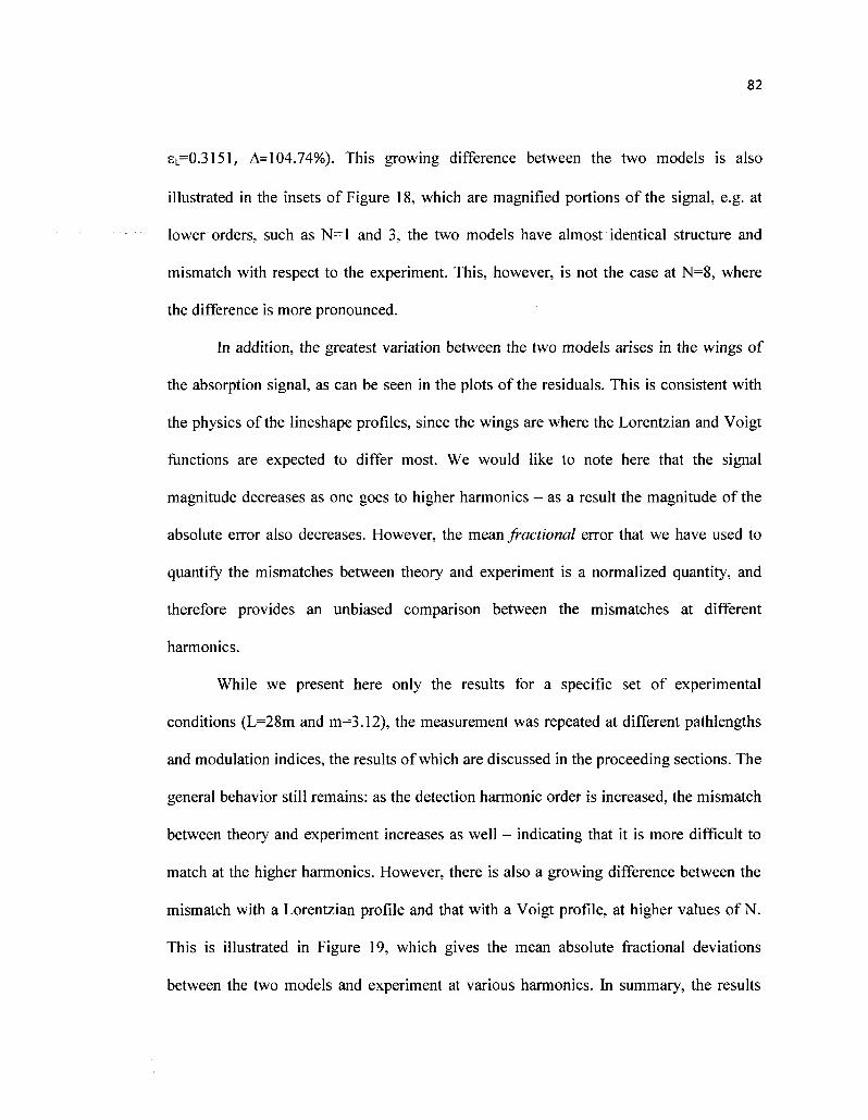
82

sL=0.3151, A= 104.74%). This growing difference between the two models is also

illustrated in the insets of Figure 18, which are magnified portions of the signal, e.g. at

lower orders, such as N=l and 3, the two models have almost identical structure and

mismatch with respect to the experiment. This, however, is not the case at N=8, where

the difference is more pronounced.

In addition, the greatest variation between the two models arises in the wings of

the absorption signal, as can be seen in the plots of the residuals. This is consistent with

the physics of the lineshape profiles, since the wings are where the Lorentzian and Voigt

functions are expected to differ most. We would like to note here that the signal

magnitude decreases as one goes to higher harmonics - as a result the magnitude of the

absolute error also decreases. However, the mean fractional error that we have used to

quantify the mismatches between theory and experiment is a normalized quantity, and

therefore provides an unbiased comparison between the mismatches at different

harmonics.

While we present here only the results for a specific set of experimental

conditions (L=28m and m=3.12), the measurement was repeated at different pathlengths

and modulation indices, the results of which are discussed in the proceeding sections. The

general behavior still remains: as the detection harmonic order is increased, the mismatch

between theory and experiment increases as well - indicating that it is more difficult to

match at the higher harmonics. However, there is also a growing difference between the

mismatch with a Lorentzian profile and that with a Voigt profile, at higher values of N.

This is illustrated in Figure 19, which gives the mean absolute fractional deviations

between the two models and experiment at various harmonics. In summary, the results

83

show that one is able to distinguish between

higher harmonics. This becomes particularly

allows for more precise characterization.

the two profiles with a higher confidence at

useful when estimating gas parameters, as it

Experimental and Theoretical

WMS Signals —Experiment —Voigt Model —Lorentzian Model

(a-1) N = 1 RQ(11,12)

Residual Discrepancies between

Theory and Experiment

— I Exp-Voigt | — I Exp-Lorentzian |

(a-2) N = 1 ev= 0.060

a ... eL= 0.071 I I A= 18.33% (A § 2-0E-3

0.76036 0.76038 0.76040 0.76042 0.76044 0.76046

Wavelength (\im)

(b-1) N = 2

0.76036 0.76038 0.76040 0.76042 0.76044 0.76046

Wavelength (urn)

(b-2) N = 2

£V= 0.0572 eL= 0.0658 A= 15.03%

< 4.0E-4

0.76036 0.76038 0.76040 0.76042 0.76044 0.76046

Wavelength (nm) 0.76036 0.76038 0.76040 0.76042 0.76044 0.76046

Wavelength (jim)

Fig. 18. Comparison of experimental WMS signals (black) with theoretical models using a Voigt profile

(green) and a Lorentzian profile (red), as well as absolute differences (residuals) for the N= 1,2...8th

harmonic of the modulation frequency. The transitions being probed are oxygen A-band RR(13,13) and

RQ(11,12) lines, with an optical pathlength of L=28m and a modulation index m=3.12. Insets are

magnified portions of the data, illustrating the growing difference between experiment and the two models.

8V and £L represent the mean absolute fractional deviations across the whole profile between theory and

experiment, when modeling with a Voigt profile and Lorentzian profile, respectively. As is the percentage

difference between ev and sL, with respect to Sy-

84

Experimental and Theoretical

25E . l n WMS Signals 1 (c-1) N = 3

0.76036 0.76038 0.76040 0.76042 0.76044 0.76046

Wavelength (urn)

Residual Discrepancies between

Theory and Experiment

2.5E-2

<D

S 2-°E-2

1 : Q 1.5E-2

Vi_-<£; IM - o

ev= 0.0647 £L= 0.0825 A= 27.51%

0.0E+0

0.76036 0.76038 0.76040 0.76042 0.76044 0.76046

Wavelength (jim)

(d - l )N=4

0.76036 0.76038 0.76040 0.76042 0.76044 0.76046

Wavelength (jim)

<B 1JE-4

c

<S iff

Q l.OE-4 a "5 o tn a < 5.0E-5 -

(d-2 N=4 ev= 0.0748 eL= 0.1138 A= 52.14%

J I 0.76036 0.76038 0.76040 0.76042 0.76044 0.76046

Wavelength (>im)

(e-1) N = 5

0.76036 0.76038 0.76040 0.76042 0.76044 0.76046

Wavelength (urn)

5.0E-5

fe 3.0E-5

(e-2) N = 5 ev= 0.1059 £L= 0.1755 A= 65.72%

MM 0.76036 0.76038 0.76040 0.76042 0.76044 0.76046

Wavelength (nm)

Fig. 18 (Continued)

85

Experimental and Theoretical

WMS Signals

Residual Discrepancies between

Theory and Experiment

(f-l) N = 6

; r 2.0E-2

GO

0.76036 0.76038 0.76040 0.76042 0.76044 0.76046

Wavelength (nm)

2.0E-5

8 c HI Qj 1.5E-5

b a 3 1.0E-S o in n <

(f-2) N = 6 8V= 0.1318 eL= 0.2111 A= 60.17%

A I 0.76036 0.76038 0.76040 0.76042 0.76044 0.76046

Wavelength (urn)

(g-1) N = 7

I 1 g l.OE-2 ^

0.76036 0.76038 0.76040 0.76042 0.76044 0.76046

Wavelength (\im)

CD 0) 6.0E-6 St

b 5 4.0E-6 o in n <

(g-2) N = 7 ev= 0.1291 eL= 0.2260 A= 75.05%

0.76036 0.76038 0.76040 0.76042 0.76044 0.76046

Wavelength (\im)

\ (h-1) N = 8

^T 8.0E-3 ra c D)

W

Ifr

0.76036 0.76038 0.76040 0.76042 0.76044 0.76046

Wavelength (nm)

(h-2)N=8 EV= 0.1539 sL= 0.3151 A=104.74 %

I 0.76036 0.76038 0.76040 0.76042 0.76044 0.76046

Wavelength (nm)

Fig. 18. (Continued)

86

U.4 -

0.35 •

. CO

2 1 a; E •g a> 0.25 -

15 S-_ UJ

S * 0-2 " •B £• o o to a> £ H 0.15 -

2 J 0.1 -ID

X )

0.05 -

0 •

• 1

i i

* Voigt model

!

i

•

i

• Lorentzian Model

•

i

]

I

I

I

\

i

1

1 1

*

i I

1 1

0 1 2 3 4 5 6 7 8 9

Harmonic Detection Order (N)

Fig. 19. Mean Absolute Fractional Deviation between theory and experiment, when using Voigt and

Lorentzian profiles, at various harmonics N of the modulation frequency. Error bars represent experimental

uncertainty. As one goes to higher detection harmonic orders, the mismatch between theory and experiment

increases. This makes any discrepancy between theory and experiment more pronounced at higher N, and

therefore such measurements put a more stringent constraint on a model. In this particular case, it is also

clear that (as would be expected under the experimental conditions) the Voigt is a better fit than a

Lorentzian. However, it is harder to come to this conclusion at low N than at higher N.

3.2.3 Effects of Increasing Modulation Index

It is well known that the modulation index, m, strongly affects wavelength

modulation spectroscopy signals. In particular, while a larger modulation index increases

the magnitudes of the signals, this is accompanied by modulation broadening which

causes a loss in features. For example, it has been shown previously [3] that while one is

able to increase the amplitude of a higher harmonic signal by increasing the modulation

index, the resulting broadening causes a loss of the features that allow one to detect

87

overlapping spectra. There is, therefore, an optimum combination of modulation index

and detection order N, needed for the resolution of overlapping lines. Experimental

results illustrating the effect of increasing the modulation index, m, on the ability to

differentiate between models are presented for N=3 in Figure 20 and N=8 in Figure 21

below.

As shown in both figures, for the same harmonic detection order and optical

pathlength, a higher modulation results in a smaller difference between the Voigt and

Lorentzian models, with respect to the experimental data. For example, in Figure 20, as

the modulation index is increased from m=3.12 to m=4.16, the difference in mean

fractional error drops from 27% to 10%. Thus, the ability to distinguish between the two

profiles is reduced. Likewise, at N=8, the same increase in modulation index decreases

the difference in mismatches from A=105% to A=86%. Hence, a smaller modulation

index results in a greater mismatch with the Lorentzian profile than with the Voigt

function.

In general, at a higher modulation index, the mismatch between the two models

and experiment are nearly identical. This reduction in sensitivity to the type of profile

assumed in the model arises from the loss in structure that occurs due to modulation

broadening. Hence, while the signal magnitude is higher at a higher value of m, the

confidence with which one can determine which model is more accurate is lower. This is

particularly visible at N=8 (insets of Fig. 21(b) and 21(c)), where the same wing, which

showed a significant difference between the two models for m=3.12, now has almost the

same theoretical values when m=4.18. Nonetheless, the overall cumulative difference at

N=8 is still significantly greater at N=8 than at N=3.

88

1.5E-1

Experimental and Theoretical

WMS Signals

—Experiment —Voigt Model —Lorentzian Model

(a-1) N=3, m=2.6

0.76036 0.76038 0.76040 0.76042 0.76044 0.76046

Wavelength (urn)

(b-1) N=3, m = 3.12

S

0.76036 0.76038 0.76040 0.76042 0.76044 0.76046

Wavelength (urn)

Residual Discrepancies between

Theory and Experiment

3.5E-4

3.0E-4

o 2.5E-4 c

§ l-OE-4

(a-2) m=2.6

ev= 0.0613

eL= 0.1026

A= 67.37%

— |Exp-Voigt| — |Exp-Lorentzian|

-J&JSJL 0.76036 0.76038 0.76040 0.76042 0.76044 0.76046

Wavelength (urn)

2.0E-2

1.8E-2

1.6E-2

" 1.4E-2

<5 St Q a 3 O J3

<

1.2E-2

1.0E-2

8.0E-3

6.0E-3

4.0E-3

(b-2) m = 3.12

ev= 0.0647

eL= 0.0825

A= 27.51%

0.76036 0.76038 0.76040 0.76042 0.76044 0.76046

Wavelength (urn)

(c-1) N=3, m = 4.16

0.76036 076038 0.76040 0.76042 0.76044 0.76046

Wavelength (urn)

i Q 3.0E-4 0) 3

(c-2)m = 4.16

ev= 0.0824

sL= 0.0910

A= 10.44%

1 0.76036 0.76038 0.76040 0.76042 0.76044 0.76046

Wavelength (urn)

Fig. 20 Comparison of experimental third harmonic WMS signals (black lines) with theoretical models

using a Voigt profile (green lines) and a Lorentzian profile (red lines), for modulation indices of m=2.6

((3=4.11 GHz), m=3.12 (P=4.93 GHz) and m=4.18 (0=6.60 GHz). The optical pathlength, L = 28m.

89

8.0E-3

7.0E-3

6.0E-3

| 5.0E-3

— 4.0E-3

O ) 3.0E-3

2.0E-3

1.0E-3

0.0E*O

Experimental and Theoretical

WMS Signals

—Experiment —Voigt Model —Lorentzian Model

(b-l) N=8, m = 2.6

h

0.76036 0.76038 0.76040 0.76042 0.76044 0.76046

Wavelength (p;m)

Residual Discrepancies between

Theory and Experiment

0) a 1-2E-6 -i t b B 3 8.0E-7 O m n <

(b-2) m = 2.6 £V= 0.1218 eL= 0.3481 A=185.79%

— |Exp-Voigt|

— I Exp-Lorentzian |

jJL M 0.76036 0.76038 0.76040 0.76042 0.76044 0.76046

Wavelength (^m)

P 8.0E-3

C 6.0E-3 g>

W 4.0E-3 •

(b-l) N=8,m = 3.12

:£\

0.76036 0.76038 0.76040 0.76O42 0.76044 0.76046

Wavelength (urn)

| , , ,

% 8.0E-4

(b-2) m = 3.12 ev= 0.1539 eL= 0.3151 A=104.74%

0.76036 0.76038 0.76040 0.76042 0.76044 0.76046

Wavelength (urn)

2.0E-2

"5 m l.OE-2 • C/3

(c-1) N=8, m = 4.16

0.76036 0.76038 0.76040 0.76042 0.76044 0.76046

Wavelength (urn)

8.0E-6

7.0E-6

0) 6.0E-6 O

O 4.0E-6 £ •§ 3.0E-6 CA

a < 2.0E-6

A

(c-2)m = 4.16

EV= 0.1392

eL = 0.2585

A= 85.70%

0.76036 0.76038 0.76040 0.76042 0.76044 0.76046

Wavelength (nm)

Fig. 21. Comparison of experimental eighth harmonic WMS signals (black lines) with theoretical models

using a Voigt profile (green lines) and a Lorentzian profile (red lines), for modulation indices of m=2.6

(p=4.11 GHz), m=3.12 (P=4.93 GHz) and m=4.18 ((3=6.60 GHz). The optical pathlength, L = 28m. The

insets illustrate the decreased difference between models at higher modulation index.

90

3.2.4 Effect of Long Optical Pathlengths

As detailed earlier in §2.3.4, pathlength saturation is an effect that occurs at large

optical depths because of non-uniform absorption across the transition lineshape profile,

for example in planetary and stellar atmospheres [46,57]. As described and presented in

detail in reference [5], the effect of this on WMS signals is a suppression of the peak at

line center with respect to adjacent peaks. Figure 22 shows a comparison of signals with

the two theoretical models, in an experiment with an optical pathlength where such

effects are visible: L=121m. The modulation index was m=3.12.

While the effect is not directly visible at the lower harmonics (N=2 and N=3 in

Figures 22(a) and 22(b), respectively), it is clearly present as a suppression of the line

center peak at N=8 (Figure 22(d)). While there is no line suppression at N=6 (Figure

22(c)), the effect is present in the form of a visible reduction of the peak height at

linecenter. Furthermore, in Figures 22(c) and 22(d), the Voigt model predicts this

depression or peak suppression effect at the line center of the RQ(11,12) line, while the

Lorentzian model does not. Pathlength saturation effects, in conjunction with higher

harmonic detection, therefore provide an additional, sensitive diagnostic for the

determination of lineshape functions.

91

8.0E-1

6.0E-1

> 15 c

—Experiment —Voigt Model —Lorentzian Model

(a) N=2

ev= 0.0463

sL= 0.0487

0.76038 0.76040 0.76042 0.76044 0.76046

Wavelength (|im)

(c) N=6

EV= 0.1254 eL= 0.1873 A= 49.36%

O.OEtO

0.76036 0.76038 0.76040 0.76042 0.76044 0.76046

Wavelength (urn)

0.76036 0.76038 0.76040 0.76042 0.76044 0.76046

Wavelength (urn)

4.0E-3

(d) N=8

ev= 0.1491 eL= 0.3038 A= 103.75%

-a^Afi^.

0.76036 0.76038 0.76040 0.76042 0.76044 0.76046

Wavelength (nm)

Fig. 22. Comparison of experimental WMS signals (black lines) with theoretical models using Voigt (green

lines) and Lorentzian (red lines) profiles, for second (a), third (b), sixth (c) and eighth (d) harmonics at high

pathlength of L=121m. (c) and (d) illustrate the suppression in peak that occurs at a modulation index of m

= 3.12. The structure of the N=6 and N=8 signals are more accurately modeled when assuming a Voigt

profile, while the Lorentzian model does not show a suppression of the central peak. While a depression is

not directly visible at N=6, the pathlength saturation effect is still present: the peak of the RQ(11,12) line is

lower than that of the RR(13,13) line (The same line has a higher amplitude at a lower pathlength as seen in

previous figures, for example in figure (18f)).

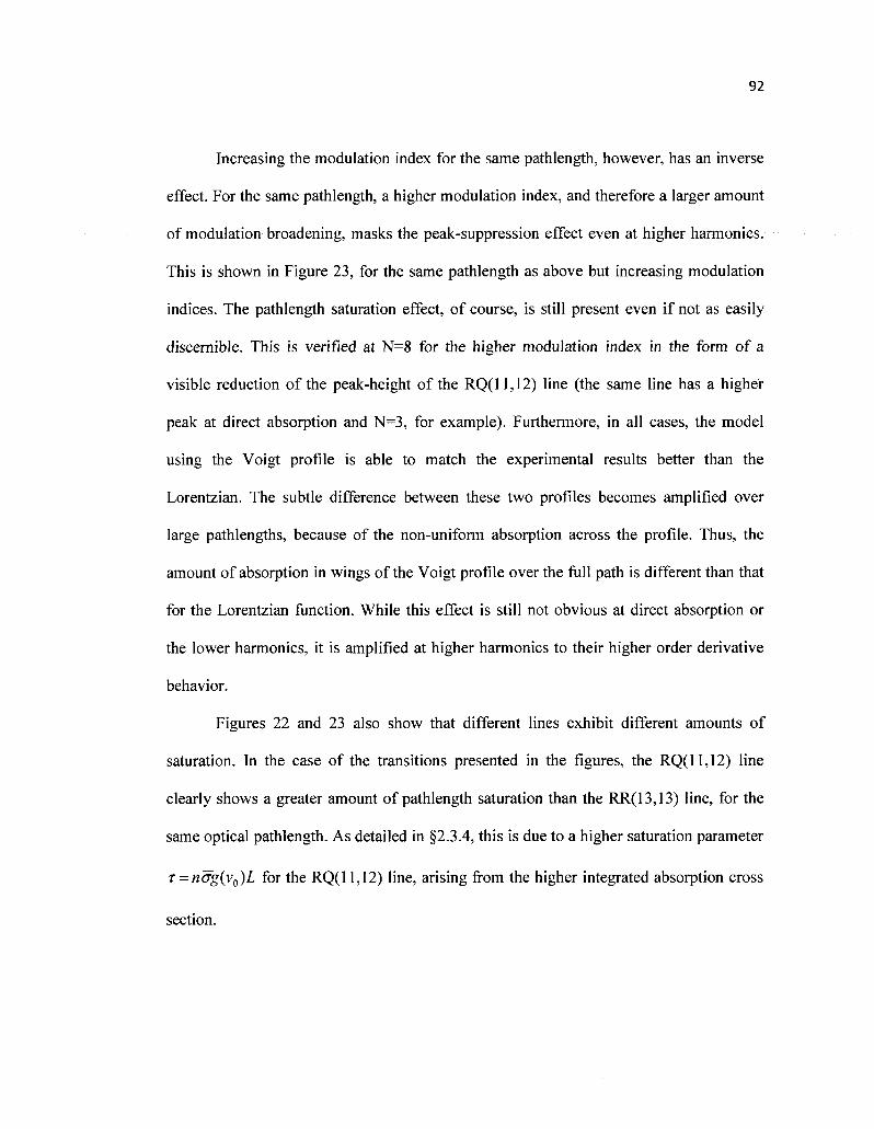
92

Increasing the modulation index for the same pathlength, however, has an inverse

effect. For the same pathlength, a higher modulation index, and therefore a larger amount

of modulation broadening, masks the peak-suppression effect even at higher harmonies.

This is shown in Figure 23, for the same pathlength as above but increasing modulation

indices. The pathlength saturation effect, of course, is still present even if not as easily

discernible. This is verified at N=8 for the higher modulation index in the form of a

visible reduction of the peak-height of the RQ(11,12) line (the same line has a higher

peak at direct absorption and N=3, for example). Furthermore, in all cases, the model

using the Voigt profile is able to match the experimental results better than the

Lorentzian. The subtle difference between these two profiles becomes amplified over

large pathlengths, because of the non-uniform absorption across the profile. Thus, the

amount of absorption in wings of the Voigt profile over the full path is different than that

for the Lorentzian function. While this effect is still not obvious at direct absorption or

the lower harmonics, it is amplified at higher harmonics to their higher order derivative

behavior.

Figures 22 and 23 also show that different lines exhibit different amounts of

saturation. In the case of the transitions presented in the figures, the RQ( 11,12) line

clearly shows a greater amount of pathlength saturation than the RR(13,13) line, for the

same optical pathlength. As detailed in §2.3.4, this is due to a higher saturation parameter

T = n<rg(vQ)L for the RQ( 11,12) line, arising from the higher integrated absorption cross

section.

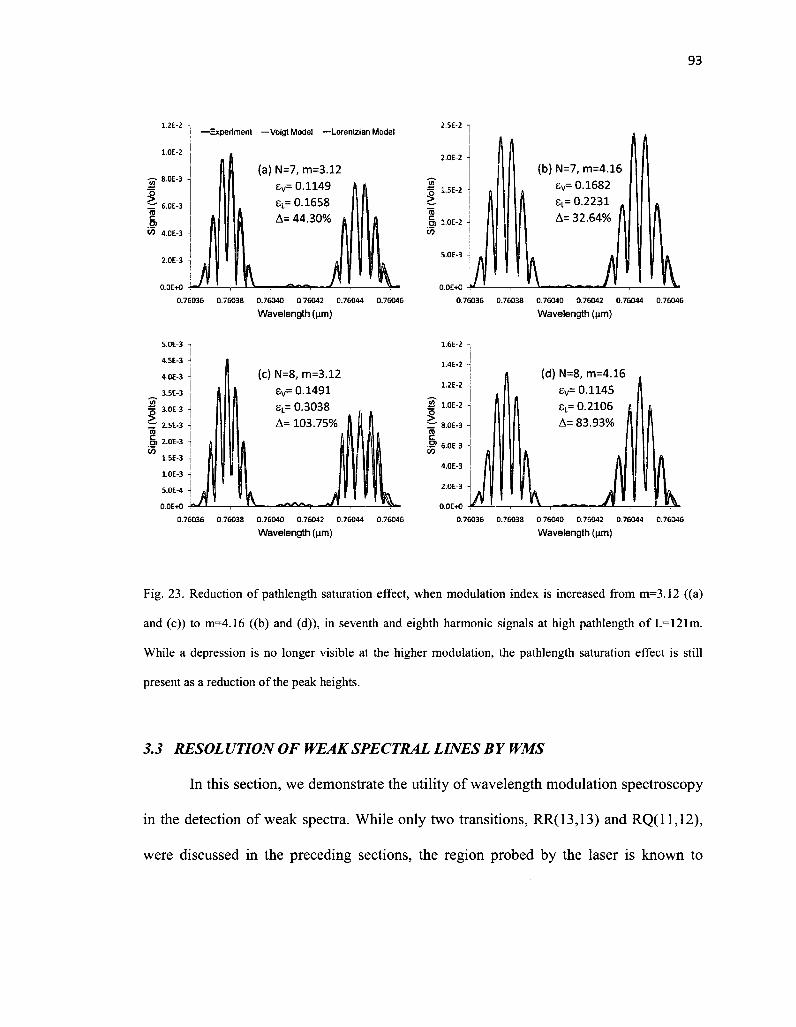
93

—Experiment —vbigt Model —Lorentzian Model

(a) N=7, m=3.12 8V= 0.1149 8L= 0.1658 A= 44.30%

0.76036 0.76038 0.76040 0.76042 0.76044 0.76046

Wavelength (jim)

(c) N=8, m=3.12 sv= 0.1491 eL= 0.3038 A= 103.75%

0.76036 0.76038 0.76040 0 76042 0.76044 0.76046

Wavelength {\im)

(b) N=7, m=4.16 ev= 0.1682 eL= 0.2231 A= 32.64%

0.76036 0.76038 0.76040 0.76042 0.76044 0.76046

Wavelength (jim)

(d) N=8, m=4.16 ev= 0.1145 £L= 0.2106 A= 83.93%

ft m. 0.76036 0.76038 0 76040 0.76042 0 76044 0.76046

Wavelength (nm)

Fig. 23. Reduction of pathlength saturation effect, when modulation index is increased from m=3.12 ((a)

and (c)) to m=4.16 ((b) and (d)), in seventh and eighth harmonic signals at high pathlength of L=121m.

While a depression is no longer visible at the higher modulation, the pathlength saturation effect is still

present as a reduction of the peak heights.

3.3 RESOLUTION OF WEAK SPECTRAL LINES BY WMS

In this section, we demonstrate the utility of wavelength modulation spectroscopy

in the detection of weak spectra. While only two transitions, RR(13,13) and RQ(11,12),

were discussed in the preceding sections, the region probed by the laser is known to

94

contain five spectral lines. Some of the additional lines that fall into our sweep, along

with their line strengths from HITRAN [39] are:

RR(13,13)*

RQ(13,13)**

RQ(11,12)*

RQ(11,12)**

RR(12,12)*

, 8 o 2

I 7 o 2

1 8 o 2

I 7 o 2

1 6 o 2

0.760355905um

0.760366631 urn

0.760412561 um

0.76041256 l|um

0.760441158um

5.77xl0"24cm2cm"

5.76xl0"24 cm2 cm"

7.66xl0"24cm2cm"

7.74xl0"24cm2cm"

6.31xl0"24cm2cm"

mol"

mol"

mol"

mol"

mol"

where the * and ** denote transitions in the lsO and 170 isotopes of molecular oxygen,

respectively. The greater nuclear mass of the isotopes results in a slight shift of the

linecenters of the same transitions. The absorption cross sections, on the other hand,

which depend on the A21 coefficient and therefore the quantum mechanical transition

probabilities, are almost the same as that for corresponding lines in 1602. However, due to

their much lower concentrations in the atmosphere (lsO has an abundance of

approximately 0.201% while that for 170 is 0.039%), these transitions are approximately

two to five orders weaker than the RR(13,13) and RQ( 11,12) transitions. Hence, the lines

are not discernible when employing direct absorption spectroscopy with the resolutions

available, as shown in Figure 24.

The direct absorption curve in Figure 24 was measured at two different optical

pathlengths, L=68m and L=121m. As can be seen from the magnified regions, the weak

transitions mentioned above are not discernible even at the higher pathlength where

absorption is stronger, either due to the systematic distortions and electrical noise, or due

to the overlap of the wings of the much stronger lines. The transitions that were included

in the calculations of the model (which used the Voigt profile) are labeled at the locations

95

they are expected to be. Rather than include all six weak transitions, we only analyzed

those that were a 100 times weaker than the "strong" lines: RR(13,13)*, RQ(11,12)* and

RR(12,12).

(b) L=68m Experiment —Model

0.76038 0.75040 0.76042

Wavelength (jim)

0.76044 0.76046 0.76039 0.7604 0.76041 0.76042

Wavelength (pm)

0.76043 0.76044

(c) L=121m

> ^ 4

* i / RR(13,13)

0.76036 0.76038 0.76040 0.76042

Wavelength ((im)

0.76044 0.76046 .76039 0.7604 0.76041 0.76042 0.76043

Wavelength (urn)

Fig. 24. Experimental (black) direct absorption signals, compared with theoretical (green) model that

includes the five labeled transitions, for pathlengths of L=68m ((a) and (b)) and L=121m ((c) and (d)).

Figures (b) and (d) are magnified portions of the absorption signals in (a) and (c). Neither the experimental

nor model data resolve the weak spectra, which are approximately two orders of magnitude weaker.

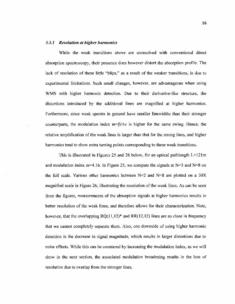
96

3.3.1 Resolution at higher harmonics

While the weak transitions above are unresolved with conventional direct

absorption spectroscopy, their presence does however distort the absorption profile. The

lack of resolution of these little "blips," as a result of the weaker transitions, is due to

experimental limitations. Such small changes, however, are advantageous when using

WMS with higher harmonic detection. Due to their derivative-like structure, the

distortions introduced by the additional lines are magnified at higher harmonics.

Furthermore, since weak spectra in general have smaller linewidths than their stronger

counterparts, the modulation index m=p/Av is higher for the same swing. Hence, the

relative amplification of the weak lines is larger than that for the strong lines, and higher

harmonics tend to show extra turning points corresponding to these weak transitions.

This is illustrated in Figures 25 and 26 below, for an optical pathlength L=121m

and modulation index m=4.16. In Figure 25, we compare the signals at N=3 and N=8 on

the full scale. Various other harmonics between N=2 and N=8 are plotted on a 30X

magnified scale in Figure 26, illustrating the resolution of the weak lines. As can be seen

from the figures, measurements of the absorption signals at higher harmonics results in

better resolution of the weak lines, and therefore allows for their characterization. Note,

however, that the overlapping RQ(11,12)* and RR(12,12) lines are so close in frequency

that we cannot completely separate them. Also, one downside of using higher harmonic

detection is the decrease in signal magnitude, which results in larger distortions due to

noise effects. While this can be countered by increasing the modulation index, as we will

show in the next section, the associated modulation broadening results in the loss of

resolution due to overlap from the stronger lines.

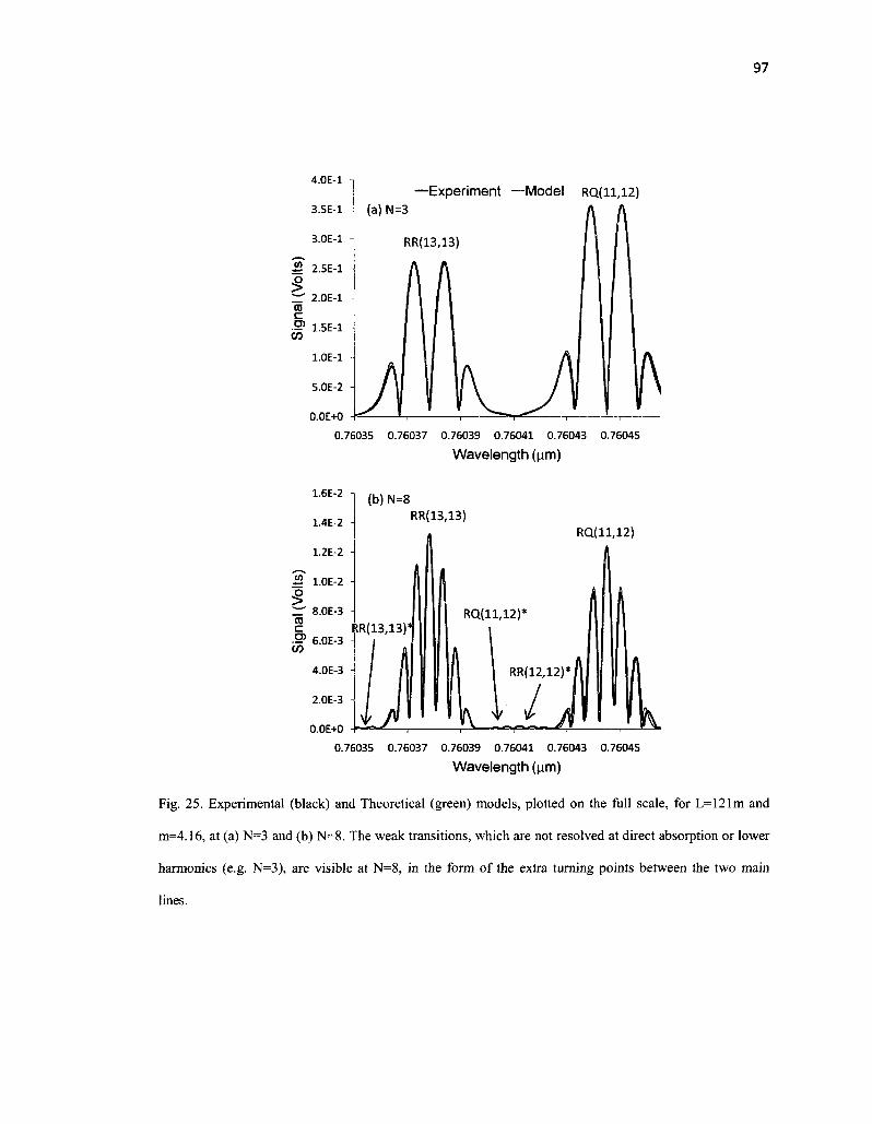
97

4.0E-1 Experiment —Model R Q ( H , 1 2 )

O.OE+O

0.76035 0.76037 0.76039 0.76041 0.76043 0.76045

Wavelength (nm)

RQ(11,12)

0.0E+0

0.76035 0.76037 0.76039 0.76041 0.76043 0.76045

Wavelength (nm)

Fig. 25. Experimental (black) and Theoretical (green) models, plotted on the full scale, for L=121m and

m=4.16, at (a) N=3 and (b) N=8. The weak transitions, which are not resolved at direct absorption or lower

harmonics (e.g. N=3), are visible at N=8, in the form of the extra turning points between the two main

lines.

98

(a) N=2 (b) N=4

0.76035 0.76037 0.76039 0.76041 0.76043 0.76045

Wavelength (nm)

(c) N=5

RQ(11,12)*

W l.OE-3

f

RR(12,12)*

O.0E*O - , ,

0.76035 0.76037 0.76039 0.76041 0.76043 0.76045

Wavelength (urn)

(e) N=7

7.0E-3

6.0E-3

3.0E-3 )

2.0E-3 -

l.OE-3

0.0E«0

I

0.76035 0.76037 0.76039 0.76041 0.76043 0.76045

Wavelength (nm)

(d) N=6

CO

0.76035 0.76037 0.76039 0.76041 0.76043 0.76045

Wavelength (nm)

(f) N=8

7? 3.0E-4 i

RQ(13,13)1 7 0.76035 0.76037 0.76039 0.76041 0.76043 0.76045

Wavelength ^m)

Fig. 26. Various harmonic signals between N=2

m=4.16. As shown, the weak spectra signals at N=£

0.76035 0.76037 0.76039 0.76041 0.76043 0.76045

Wavelength (nm)

to N=8, on a 30X magnified scale, for L=121m and

are better resolved than at lower harmonics.

99

3.3.2 Effect of Modulation Broadening

As discussed earlier, a higher modulation index results in a higher signal

magnitude. However, increasing the modulation index also results in a broadening of the

harmonic signals. Hence, any weak lines that might be resolved at a low modulation

index at some particular harmonic, may no longer be as resolved with a higher

modulation index, due to the loss of structure caused by the broadening. This effect is

illustrated in Figure 27, which plots the signals on a 30X magnified scale between the

two strong transitions for different modulation indices at a pathlength of 75m.

For example, when looking at the signal at N=4, increasing the modulation index

from m=3.12 to m=4.16 results in an almost complete loss of the weak RR(13,13)* and

RQ(11,12)* signals - one loses almost all distinguishing turning points that suggest the

presence of an additional line. This loss in the number of turning is also seen at N=5 for

the same change in modulation index. Likewise, the weak spectra at N=6 experience a

decrease in magnitude relative to the overall signal magnitude.

While higher harmonic signals provide greater resolution of the diffuse spectra,

signals get significantly weaker as N increases. At some point, the amount of noise

present compared to the signal magnitude becomes relevant and may override the signal

being sought. This is normally countered by increasing the modulation index, which,

however, results in a broadening of the spectra. As a result of this broadening, the

stronger lines may overlap and hide the weak transitions. Thus, an optimal balance

between harmonic order and modulation index is required when resolving weak spectra

with WMS,

100

m=3.12

(a-1) N=4

0.76035 0.76037 0.76039 0.76041 0.76043 0.76045

Wavelength (^m)

(b-1) N=5

0.0E+O

RQ(11,12I*

0.76035 0.76037 0.76039 0.76041 0.76043 0.76045

Wavelength (jim)

(c-1) N=6

RQ( 11,12)'

0.76035 0.76037 0.76039 0.76041 0.76043 0.76045

Wavelength (urn)

m=4.16

(a-2) N=4

P 4.0E-3

RQ111,12)*

0.76035 0.76037 0.76039 0.76041 0.76043 0.76045

Wavelength (jim)

(b-2) N=5

0.76035 0.76037 0.76039 0.76041 0.76043 0.76045

Wavelength (|im)

(c-2) N=6

^ 2-0E-3

I iT' 1.5E-3 c .•> "3 1.0E-3

RQ(11,12)*

0.76035 0.76037 0.76039 0.76041 0.76043 0.76045

Wavelength (jim)

Fig. 27. Comparison of the resolution of weak spectra at (a) N=4, (b) N=5 and (c) N=6l harmonic of the

modulation frequency, when the modulation index is increased from m=3.12 to m=4.16. The resulting

modulation broadening causes a loss in the relative amplitudes and numbers of extra turning points that

indicate the presence of the weak transitions.

101

CHAPTER IV. INFORMATION INHERENT IN THE STRUCTURE

OF SIGNALS

One common theme in all of the work presented in this dissertation has been the

extraction of information from the structure of signals. In the previous sections, for

example, information about weak spectra was contained in the structure of the absorption

profile, the finer features of which we were able to discern at higher harmonics.

Likewise, the higher sensitivity of higher detection orders allowed us to differentiate

between two profiles that are otherwise very similar in conventional direct absorption

spectroscopy. All the information about a radiating or absorbing source can be

determined from its absorption or emission frequency spectrum. For example, one can

obtain a measurement of temperature, pressure, collision dynamics, etc. from an accurate

measurement of the linewidth of the lineshape profile.

While the preceding arguments are made about distributions in the frequency

domain, one can obtain information from a target by examining various regions of any

relevant phase space. For example, the classical Young's double slit experiment carries,

in the spatial distribution of the fringes, information about those slits, in particular the slit

separation and slit width, and, were either of those to change, the spatial distribution of

the fringes would also change. Likewise, as we show in this chapter, one can obtain

information about the parameters of a classical antenna array by studying its spatial

distribution of power, i.e. the radiation pattern.

However, many questions arise in any such measurement, including: "What is the

maximum amount of information - in bits - that can be extracted using the experimental

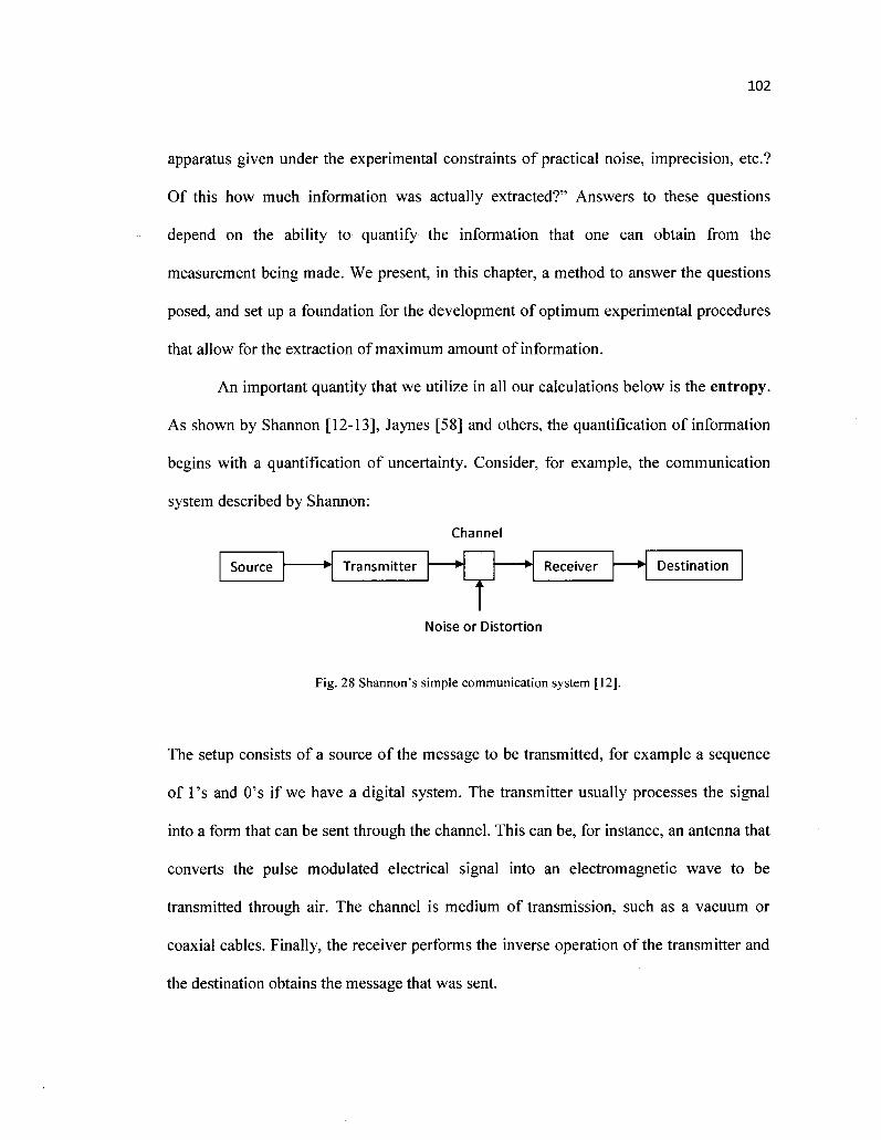
102

apparatus given under the experimental constraints of practical noise, imprecision, etc.?

Of this how much information was actually extracted?" Answers to these questions

depend on the ability to quantify the information that one can obtain from the

measurement being made. We present, in this chapter, a method to answer the questions

posed, and set up a foundation for the development of optimum experimental procedures

that allow for the extraction of maximum amount of information.

An important quantity that we utilize in all our calculations below is the entropy.

As shown by Shannon [12-13], Jaynes [58] and others, the quantification of information

begins with a quantification of uncertainty. Consider, for example, the communication

system described by Shannon:

Channel

Source Transmitter Receiver Destination

Noise or Distortion

Fig. 28 Shannon's simple communication system [12].

The setup consists of a source of the message to be transmitted, for example a sequence

of l's and O's if we have a digital system. The transmitter usually processes the signal

into a form that can be sent through the channel. This can be, for instance, an antenna that

converts the pulse modulated electrical signal into an electromagnetic wave to be

transmitted through air. The channel is medium of transmission, such as a vacuum or

coaxial cables. Finally, the receiver performs the inverse operation of the transmitter and

the destination obtains the message that was sent.

103

In this system, there are many locations where uncertainty could arise. For

example, the transmitter may be riddled with systematic processes that distort the signal

being sent to the destination. The presence of noise in the channel is also a big

contributor to uncertainty of the message being transmitted exactly. It is this uncertainty

that allows for the transmission of information; for if one knew everything about the

properties of the message, then there is no information to be transmitted. However, any

real physical process will always have some uncertainty associated with it, and the

reduction of this uncertainty is the information that one extracts. [12-13,58].

The uncertainty is quantified as information in terms of number of arrangements

[12-13,58-60]. Consider the very simple example of a box containing Ni red balls, N2

blue balls, and N3 green balls, where Ni is some very large number. Suppose also that the

box contains a total of N=Ni+N2+N3 slots. Thus, if the box is "shaken up," the balls will

fall into the slots in some particular arrangement, which we see if we open the box and

look. By "looking" in the box, i.e. making the measurement, we remove all uncertainty

and obtain information about the balls. However, prior to making the measurement, our

uncertainty depends on the number of arrangements, W, given by:

N! W = : (79a)

N,!N2!N3!

Since the number of balls is large, we employ the Stirling approximation N!« NNe"N .

Thus, the number of arrangements is approximately:

104

w* N N e - N

( N / V N ' ) ( N / V N 0 1 N 3 * V N 3 ) N N , + N 2 + N 3 e - N , e - N 2 e - N 3

(N1N 'e-N>)(N2%-^j(N3

N3e-N3)

/'XT "\ N v N y

N, / ^ r N-N

N OO v N y (79b)

where pi is the probability of obtaining the i-th ball. One can easily see from this that

maximum number of arrangements occurs when we have equal numbers of each color

ball, i.e. pi=p2=p3=l/3. Defining the entropy, H, as the log of number of arrangements per

outcome, as was done by Boltzmann and others for convenience purposes [12-13,60], we

obtain:

H = -Xp ilog(Pi) (80) i

which has the units of bits when the logarithm is taken in base 2 units, or nats if

calculated using natural logarithms. Hence, in this example, if the number of red, blue

and green balls is equal, then the act of opening the box and "measuring" results in a gain

of ln(3) nats of information. This definition and approach of entropy was used by James

Maxwell and Ludwig Boltzmann when deriving their distribution of gas molecules at

thermal equilibrium [60-61]. In fact, thanks to the efforts of the likes of Jaynes [58-59],

Landauer [62] and Bennet [63], we now appreciate that the entropy of information theory

is physically identical to that of thermodynamics.

The above arguments involving the measurement of arrangements of balls can

now be extended to communication systems as well. Instead of referring to the color of

the ball, we can instead define it as a state of the ball. Consider for example a simple

transistor, which operates in two states. If one has a very large number of transistors, or

105

equivalently operates one transistor to give a sequence of on and off states, the

arrangements of 1 and 0 states serves as a message of the kind in Shannon's

communication system. If the probability of the two states is equal, then by measuring the

state of a transistor, we obtain exactly 1 bit or ln(2) nats of information. On the other

hand, if we start with some precise sequence of 1 s and Os as a message, and a systematic

process in the channel or even random noise distorts that message, then we lose

information. Also consider a distribution of photons in space. Suppose that one is given

the probability density function with which photons are emitted at some azimuthal angle;

in this case, the entropy is a measure of the number of ways the distribution can be built

up - that is, the number of ways the spatial signal can be generated. Likewise, if we have

a distribution in frequency, then the entropy of that distribution measures the number of

arrangements in which that frequency profile may be built up.

Having defined the entropy, we will now calculate the information that one

obtains about a particular parameter by reducing the uncertainty. We will treat two cases:

the first is that of information about the phase of an antenna array radiation pattern, which

is a spatial distribution of photons. The second case that we treat involves the precise

measurement of frequency from higher harmonic signals. While the calculation will be

done for these two specific cases, the method described is general and can be extended to

any physical distribution in the relevant phase space.

106

4.1 INFORMA TION FROM ANTENNA RADIA TION PA TTERNS

We will examine, in this section, the amount of information that one obtains from

the radiation patterns of coherent antenna arrays. These are coupled systems of individual

antennas, which generate various spatial distributions of the radiated power (i.e. radiation

patterns), are useful in a wide variety of applications, such as beam steering or optical

sensing [64-65]. We calculate the information that one extracts by determining the phase

of an antenna array, by measuring the location of the maxima or minima of the radiation

pattern. The radiation pattern of a linear one-dimensional phased array is given by [1]:

PM<t>) = Pmd(e,$y ^ Qxp{j(kd, sin 0 sin <j> + y/,)} (81)

where Pind is the power distribution in the pattern of an individual antenna element, k is

the wave number, di is the spacing between the n individual elements of the array and *Pi

is the phase of the current driving the Ith current element. P„(0, <f>) is the power emitted per

unit solid angle in the direction (9, <j>).

The parameters of the phased array, such as the number of radiating elements, the

driving currents of each element, the relative phases between the elements, etc. can all

therefore be determined by measuring the array's radiation pattern, fully described by

(81). In this section, we discuss the determination of the inter-element phase by

measurement of the locations of maxima and minima of the radiation pattern. Let us

assume that the spacing between all the elements of the array is the same and fixed, d,

and let us also assume that the phase between the elements is the same and fixed, VF. Such

arrays, most commonly referred to as simple uniform phased arrays, have a radiation

pattern given by:

107

. 2jn(kd sin 0 sin <f> + (//)]

PtfJ) = PmM<l>) >/, , • / • , r f (82) -2J (kdsin<9sin^ + (//)| ' I 2

sin

The maxima of this radiation pattern occur at:

(kd sin 6 sin d> + u/} n

—— = u,n,2n,... 2 kd sin 9 sin <f> + if/ = 0,27i,47r,... = 2a7r (83a)

a = 0,1,2,....

while the minima occur when:

(kd sin 0 sin (i + u/) n

2

kd sin 6 sin (j> + y/ -2n I n,4n /«,... = 2an I n (83b)

fo/sin^sin^ + z 0,27r,4;r,... = 2(2 -

or = 0,1,2,....

Thus, knowing the exact location (G, ((>) of a maximum or minimum, one can

determine the phase ¥ of the array to infinite precision (keeping in mind the 2TC

periodicity). However, if there is an uncertainty in the measurement of this location, there

arises a corresponding uncertainty in the measured value of the phase. Such an

uncertainty will arise if, for example, the detectors covering the 4n space to measure the

radiation pattern are of some finite size. Hence, in that case, one can only specify the

location of a maximum or minimum to within some finite tolerance. A similar uncertainty

would arise if due to electrical noise, one is only able to define a maximum or minimum

over some range of values.

This is illustrated in Figure 29 below. Figure 29(a) shows the radiation pattern of

an array with n=2 elements, d = R and a phase that is initially VF0=0°, when measured with

108

an infinite number of infinitesimal detectors, the ideal - but obviously physically

unattainable - case. Figure 29(b) shows the radiation pattern measured in this idealized

case when the inter-element phase changes to ¥=20° (i.e., there is now a phase difference

of 20° between the excitation currents of the two antennas).

Figures 29(c) and 29(d) illustrate the same radiation patterns in Figures 29(a) and

(b), but when measured with finite sized detectors, each having a span of A<))=10o. We

observe from Figures 29(a) and (b), that when the phase changes from 0° to 20°, the

maximum that occurred initially at location <j>=0° has moved slightly to (j>=-3.18°. This

change, however, is not registered in the case when the radiation pattern is measured with

the finite sized detectors - the detector centered at §=0° will still register a maximum, and

therefore cannot determine whether the phase of radiating array has changed. Likewise,

the minimum (a null in this case) that occurs at (j>=30° when ^¥=0°, now occurs at (|>=26.40

when the phase changes ¥=20°. Again, the finite sized detector fails to register a change,

and therefore does not register the change in VF.

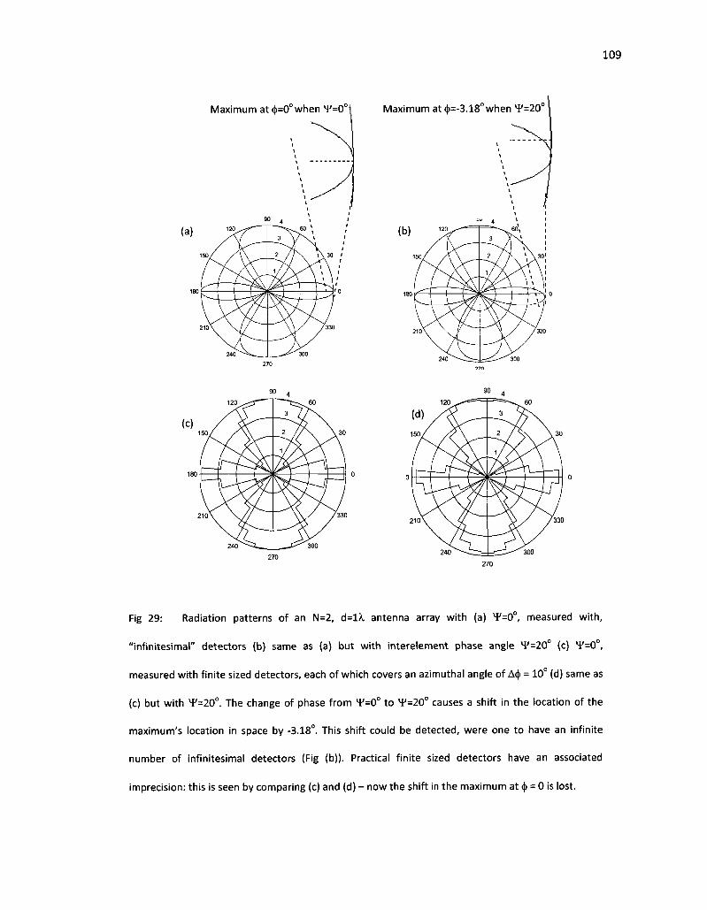
Fig 29: Radiation patterns of an N=2, d=lX antenna array with (a) V=0°, measured with,

"infinitesimal" detectors (b) same as (a) but with interelement phase angle ¥=20° (c) ^¥=0°,

measured with finite sized detectors, each of which covers an azimuthal angle of A§ = 10° (d) same as

(c) but with 4/=20°. The change of phase from ¥=0° to ¥=20° causes a shift in the location of the

maximum's location in space by -3.18°. This shift could be detected, were one to have an infinite

number of infinitesimal detectors (Fig (b)). Practical finite sized detectors have an associated

imprecision: this is seen by comparing (c) and (d) - now the shift in the maximum at (|> = 0 is lost.

110

From equations (83), we can therefore determine the range of phase values,

AT, over which the location of a maximum or minimum will be indistinguishable, when

the radiation pattern is measured with finite sized detectors as opposed to infinitesimal

ones. That is, if the phase of the current source driving the array fluctuates over AT, a

change in the location of a maximum or minimum of the radiation pattern measured will

not be observed over that detector. Thus, for a given finite sized detector placed at a

location where the radiation pattern has a maximum or minimum, we have a uniform

probability density function, p(iF)=l/Ax¥, of phase values that will register a maximum

or minimum for that detector [1]. Using the continuous limit of the definition of entropy,

the entropy of this phase distribution is given by:

H(At) = -\p(y)lnp(y/)dV, (84)

This entropy is a measure of the number of arrangements by which the possible

phase values could be distributed, but of which the measurement would yield no

information. To appreciate the meaning of the entropy as applied to our problem, assume

that instead of a continuous distribution, our current source fluctuations occur in phase

values that can only be any one of 360 values (i.e. 1°,2°,....360°). Hence, instead of an

infinite number of phase values within AT, we now instead have a finite number of phase

values - and a discrete probability distribution, p(T).

While we have chosen to assume that any one of only 360 values are possible for

illustrative purposes, we find that this can be any value, and in the limit that the

separation goes to zero, we arrive at the entropy measure for a continuous probability

I l l

density function p(vF) given by Equation (84). The entropy of this discrete probability

distribution, pOF), is thus given by Equation (80):

H{^) = -Ydp{ilf,)hip{y/t) (85)

where m is the number of discrete phase values in the interval, AT, over which the

excitation currents fluctuate.

We can now obtain an expression quantifying the amount of information that can

be gained when one set of finite sized (represented by A<j>i) detectors are replaced by

another set of finite sized (Afo) set. We apply (85) to three sets of detectors (A<|> = 1°, A(|>i,

A<j>2; A<|>i, A(|>2 assumed > 1°- just for the sake of the current discussion). The additional

information that would be obtained by going from detectors A<j>i to A<|> = 1° is H(A(j)i)-

H(A(|>=10). While in the imprecise case that A<j>i had many possible values of phase in a

distribution p(T), the precise case, A<j)=l°, gives us one exact value of T. Similarly, the

additional information that would be obtained by going from detectors of size A<j>2 to A<(> =

1° is H(A(|)2)-H(A(|)=10).

In this way, the information in nats, (or with a change in scale, in bits) improving

detection precision when going from detector size Afoto Ac|>i (with A<j>2 > A(j>i) is

AH = H(A<t>2)-H(A0l) (86)

While the discussion leading to (86) assumed that the phase only takes discrete values

within AT, the expression for information obtained, given by equation (86) remains the

same as we approach the continuous limit where all values in AT are possible. As shown

112

by Shannon [12-13], we may rewrite equation (85) in terms of a probability density

m

function, pQ¥), as//(A^) = -^jp(V/,)AV/i l n ^ , ) ^ , ] , where p C F , ^ , = pO^).

Equation (86) therefore becomes: m m

AH = -]rp(y/.,A<z>2)A<//,ln[p(y,, A^2)A(//,] + £/7(y/,, A^)Ai//,An[/?((//, A?*,) Ay/,] ;=1 (=1

In the limit that A*F -> dT, the summation becomes an integral:

AH-- \p(i//,A<f>2)\np(y/,A02)dy/- \p(i//,A02)ln(Ai{/)dtj/ Ay-> A /->

+ ^p(y/,A<f>])\np(iy,A<f>l)di//+ jp(y/,A^)h(Ay/)dy/

= - J/^,A^2)lnp(y/,A^2)^-ln(A^) ^p(i//,A</>2)di{/

+ \p(i//,A^)\np(y/,A^)dy/ + \n(Ay/) \p{ii/,A(l>})dy/

= - J^A^lnpO^A^^-lntAy/)

+ J/9(i/ A(0,) In/?((//, A^)d^ + ln(A^) A(c,

= - jp( ,A 2)ln/?( ,AfzS2)<fy/ + Jp((//,A^)lnyO(^,A^)^

.\A// = i /(A&)-//(A^)

which is exactly equation (86), but for a continuous density function of phase values.

Shannon, in his fundamental papers [12-13], discusses an important aspect of the entropy

of continuous distributions. Upon inspection of equation (84), we find that there is a

dimensions mismatch, i.e. the logarithm term is not dimensionless. In fact, the limit to a

continuous distribution of the discrete entropy given by equation (85) results in equation

(84) plus an infinite term. However, as Shannon, and remarkably Einstein in an earlier

113

paper [66], mention, taking a difference of entropies as done in (86) solves the dimension

problem.

Hence, H(A<|>), as defined by equation (84) is the amount of information one

obtains when replacing the finite sized detectors, of size A<|>, which result in a range of

values of *¥ with probability distribution pCF), with ideal (but not practical in reality)

infinitesimally precise detectors that result in one exact value of the phase VF. The amount

of information that can be gained when one set of such finite sized (represented by A<j>i)

detectors are replaced by another set of finite sized detectors (A^) is thus given by

equation (86).

Results of the calculation of the information that one obtains when going from the

most imprecise detector, given by size A(|>2 = n, to a more precise detector of size A<J>15 are

given in Figures 30 and 31 below. In the most uncertain scenario, A(j>2, the range of

phases is from y¥=-n to y¥=n, or Ai¥=2n and the entropy of this case, which serves as our

reference in the subtraction in equation (7), is given by ln(27i). The calculations in Figure

30 are performed for the case of N=2, d=lA, and for an initial phase of T=0. The

information obtained is calculated for different detector sizes, A<|>i, at three different

locations of the detector: a detector placed at the maximum at <|)=0o; at the maximum at

<t>=90°, and for the minimum at § = 30°. Since the radiation pattern is symmetric, the

results in the first quadrant apply to all four quadrants. Likewise, in Figure 31, we

calculate the information obtained about phase for the case of N=3, d=lA. and for an

initial phase of^M). In this case, we have two additional nulls between the major lobes.

114

From the figures, it can be seen that the most amount of information, for a given

detector size, is obtained when measuring the maximum at <|> = 90°. This corresponds to

the location with the smallest range of possible phases, A*¥, such that a maximum (or

minimum) is still measured on the detector. In all three cases, no information is obtained

when the size of the detector is such that the range of possible phases is 2n. This situation

occurs at different detector sizes for the different locations, due to the different sensitivity

to phase changes at these respective locations - i.e. if the detector is larger than a certain

size, one obtains zero information about the phase beyond this point, when compared to

using the most imprecise detector (A§2 = n, i.e. 180°).

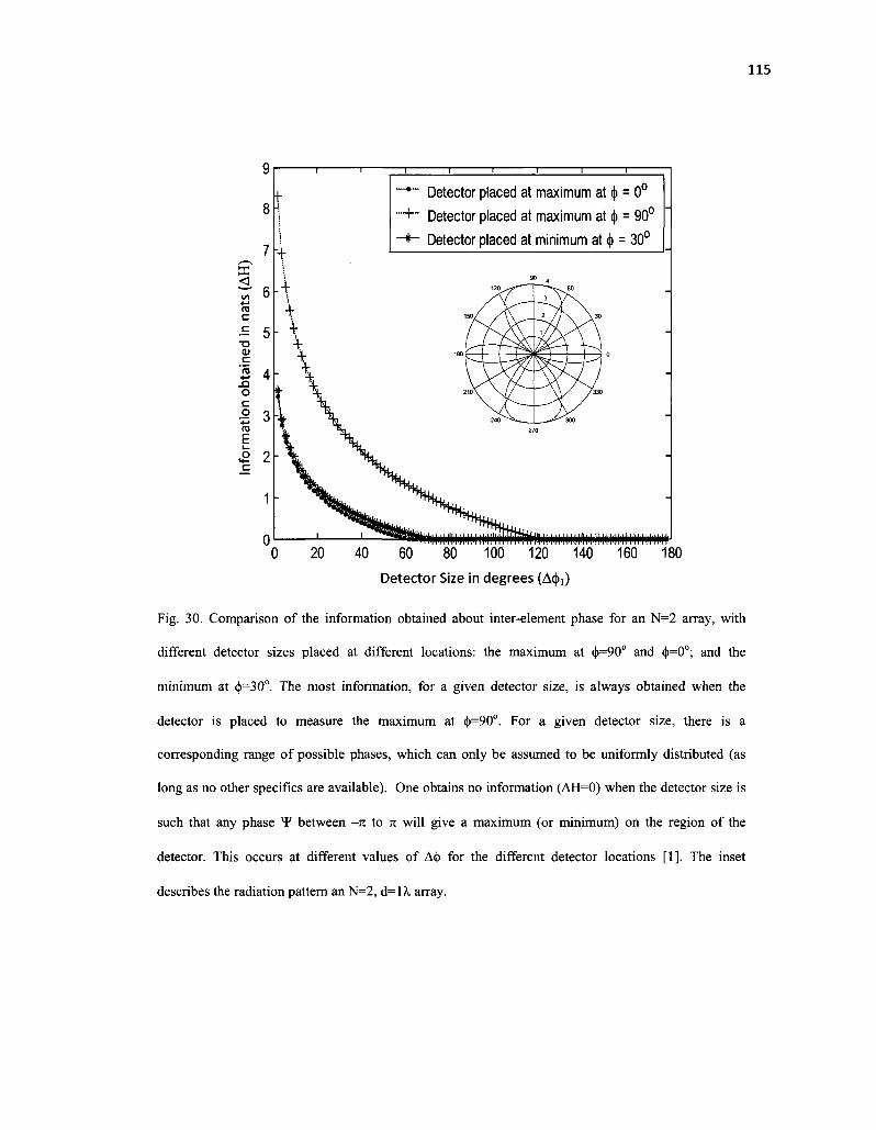
< ~ 6 4-* TO

C

•£ 5

3 4 - Q O C

£ £ 2 c

k- Detector placed at maximum at <|> = 0°

Detector placed at maximum at <|> = 90°

Detector placed at minimum at § = 30°

0 20 40 60 80 100 120 140 160 180

Detector Size in degrees (A<|>i)

Fig. 30. Comparison of the information obtained about inter-element phase for an N=2 array, with

different detector sizes placed at different locations: the maximum at (|>=90o and (j>=0o; and the

minimum at <j)=30°. The most information, for a given detector size, is always obtained when the

detector is placed to measure the maximum at <|>=90o. For a given detector size, there is a

corresponding range of possible phases, which can only be assumed to be uniformly distributed (as

long as no other specifics are available). One obtains no information (AH=0) when the detector size is

such that any phase *¥ between -n to n will give a maximum (or minimum) on the region of the

detector. This occurs at different values of A<|) for the different detector locations [1]. The inset

describes the radiation pattern an N=2, d=lX, array.

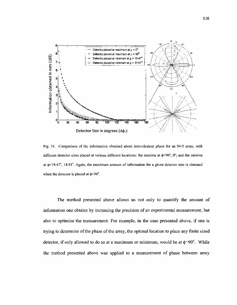
116

Fig. 31. Comparison of the information obtained about inter-element phase for an N=3 array, with

different detector sizes placed at various different locations: the maxima at 4>=90°, 0°; and the minima

at (|)=19.47°, 14.81°. Again, the maximum amount of information for a given detector size is obtained

when the detector is placed at (|>=90o.

The method presented above allows us not only to quantify the amount of

information one obtains by increasing the precision of an experimental measurement, but

also to optimize the measurement. For example, in the case presented above, if one is

trying to determine of the phase of the array, the optimal location to place any finite sized

detector, if only allowed to do so at a maximum or minimum, would be at 4>=90°. While

the method presented above was applied to a measurement of phase between array

117

elements, it may be extended to a measurement of other parameters such as inter-element

spacing, driving currents, etc.

Furthermore, while the above discussion was aimed at an antenna array and the

information that the radiation pattern of such an array carries, the method holds for any

system, which is monitored in its appropriate phase space. Hence, for example, one can

do an analogous treatment of the emission (or absorption) frequency spectrum of an atom

or molecule, or any remote sensing technique, including wavelength modulation

spectroscopy.

4.2 INFORMA TIONIN THE STRUCTURE OF WMS SIGNALS

Just as the uncertainty in location of the maxima or minima of an antenna array's

spatial photon distribution led to an uncertainty in the inter-element phase, uncertainty in

measurement of the frequency spectrum can lead to uncertainty in the linewidth. Since

the linewidth is dependent on various parameters, such as temperature, collision cross-

section, etc, these parameters will have associated range of possible values as well. We

will now apply the method described in §4.1 to calculate the information that one can

extract from the experimental wavelength modulation spectroscopy signals, described in

Chapter 3 [19].

Suppose one is attempting to estimate the collision linewidth contribution to the

Voigt profile (and therefore the collision cross-section) of the RQ(11,12) line, shown in

Figures 18 and 20, by matching the theoretical model to experimental data. At any

particular detection order, there will be a range of collision linewidth values that give a

model that matches the experimental data within a given tolerance. There is, therefore, an

118

uncertainty in the value of the linewidth. Likewise, at a different harmonic order, one will

have a different range of linewidths that gives a match between theory and experiment

within the same tolerance. This range of collision broadened widths in the second case

may be larger or smaller than the first case. Thus, in the process of going from the first to

the second case, one reduces or increases the uncertainty in the value of linewidth,

obtained from matching a theoretical model to the experimental data. This is analogous to

the uncertainty in the phase between inter-element driving currents in antenna arrays.

This decrease or increase in uncertainty may also be quantified as a gain or loss of

information about the linewidth, as done in §4.2.

The result of such a calculation for the RQ( 11,12) line at different modulation

indices and pathlengths is shown in Figure 32. Plotted are the range of allowed collision

linewidths around the nominal value of Sv2coll= 1.586 GHz, that give a tolerance of 15%

between theory and experiment for the RQ( 11,12) line, at different harmonic orders N.

We observe a reduction in the range of linewidths that give a less than 15% match as one

performs higher harmonic detection, consistent with the results of increased sensitivity at

higher harmonics given in §3.2. Furthermore, the modulation broadening at higher

modulation index results in a smaller sensitivity, and therefore larger range of allowed

model widths.

Given no other constraints, we assume that the linewidth values over this range

are distributed uniformly - that is, all values within the range of linewidths are equally

likely. Hence, the information obtained when determining the linewidth at some detection

order with respect to direct absorption (N=0) is given by:

I = ln{range(N = 0)}- ln{range(N)} = -ln{range(N)/range(N = 0)} (87)

119

The results of this calculation are plotted in Figure 33 and show a gain in the amount of

information about the collision linewidth when one makes the measurement at a higher

harmonic order. This effect is a direct consequence of the larger amount of structure of

higher harmonic WMS signals (as exemplified by the larger number of turning points and

zero crossings), which makes them more sensitive to smaller differences in linewidth,

compared to the lower order harmonics. Furthermore, since signals at a higher pathlength

are more sensitive to changes in linewidth, the amount of information obtained is larger.

1.6 -]

„ 1A • JZ

2 , , i • m=3.12, L=121m g 12 1 • m=4.18, L=28m

g i.o ^ ' ± m=3.12, L=28m

"o • o 0.8 -j

TJ . <U *

M 0.G ^ CD

| 0.4 J

i ! a i . -

0.2 ; •

0.0

0 1 2 3 4 5 6

Harmonic Order (N)

Fig. 32. The range of allowed collision linewidths, as a function of the harmonic order. Detection at

higher harmonics yields a narrower range of widths that result in an up to 15% match between model

and experimental data. The modulation broadening at higher modulation index results in decreased

sensitivity and a larger range of allowed collision widths.

c o

o to ro +-• u

> i/5

•S « 3

_c +-"

$ 2

c o

1 1 I -

c

• m=3.12, L=121m • m=3.12, L=28m A m=4.18, L=28m

3 4 5 6 7

Harmonic Order (N)

Fig. 33. Information obtained vs. Harmonic order, with respect to direct absorption when estimating

the collision linewidth with a 15% tolerance between model and experimental results. Different

modulation indices and pathlengths are shown, with the results consistent with the increase in

sensitivity at increased pathlength and decreased modulation index, shown in §3.2.

Thus, we have quantitatively shown that despite a decrease in the amplitude of

the signals, the higher sensitivity of high harmonic signals due to their larger amount

of structure (N zero crossings and N+l turning points) allows for the extraction of

more information about the linewidth parameter. This approach may be extended to

other parameters, as well as even higher detection orders greater than N. Ultimately,

due to distortions from noise, one is expected to arrive at some optimum order, N.

121

4.3 THERMODYNAMICS OF INFORMATION LOSS IN LINESHAPE

MEASUREMENTS

The relationship between information loss and heat generation is a well known

one. For example, Landauer [62], Bennet [63], and others have shown that at the

fundamental level, a minimum amount of heat equivalent to kTln2 is generated when 1

bit of information is erased. Hence, the question "How much information, in bits (or

nats), is lost when making a practical measurement and how much heat is generated in

the process?" arises. This is a fundamentally important question to answer in any

experimental measurement that strives to achieve the highest precision possible. In this

section, we calculate the information lost in a practical multi-channel spectral analyzer,

where the lineshape profile measured is averaged. This occurs due to the finite frequency

resolution of the device. We also present a calculation of the heat generated in the

photodetector in this system, and examine its connection to the information lost [14].

To model this situation, let us consider an optical experiment in which an

emission signal is measured by a multi-channel spectral analyzer (a basic grating

sprectrometer), illustrated in Figure 34 below. A diffraction grating scatters the emission

spectrum at various angles according the respective frequencies of the photons. The "exit

holes" at each angle are calibrated to the corresponding frequency intervals, and a

photodetector behind each exit hole counts the number of photons emitted in that

particular frequency interval. In addition, the bandgap of every photodetector is finely

tuned to the lower end of the corresponding frequency interval. This is to prevent any

excessive heat generation due to the relaxation of electron-hole pairs via phonon modes.

One can, therefore, measure the emission lineshape profile in this manner by measuring

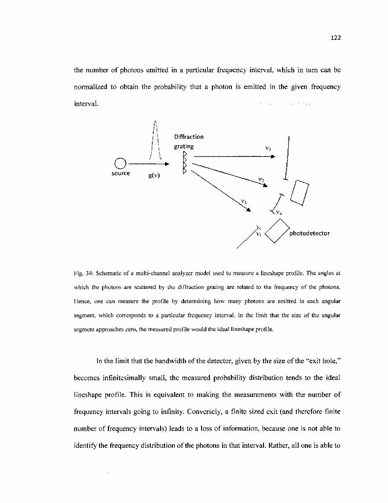
122

the number of photons emitted in a particular frequency interval, which in turn can be

normalized to obtain the probability that a photon is emitted in the given frequency

interval. -

O source

Diffraction

grating

g(v)

photodetector

Fig. 34: Schematic of a multi-channel analyzer model used to measure a lineshape profile. The angles at

which the photons are scattered by the diffraction grating are related to the frequency of the photons.

Hence, one can measure the profile by determining how many photons are emitted in each angular

segment, which corresponds to a particular frequency interval. In the limit that the size of the angular

segment approaches zero, the measured profile would the ideal lineshape profile.

In the limit that the bandwidth of the detector, given by the size of the "exit hole,"

becomes infinitesimally small, the measured probability distribution tends to the ideal

lineshape profile. This is equivalent to making the measurements with the number of

frequency intervals going to infinity. Conversely, a finite sized exit (and therefore finite

number of frequency intervals) leads to a loss of information, because one is not able to

identify the frequency distribution of the photons in that interval. Rather, all one is able to

123

obtain is the total number of photons and the frequency interval in which those photons

fall. There is therefore a loss of information in the distribution of the photons, with

respect to frequency. Again, because we are not privy to any further knowledge about the

distribution of the photons in the frequency interval, we assume it to be uniform (which is

the most unbiased distribution under these conditions [58-59]). Hence, there is a loss of

structure of the lineshape profile, as illustrated in Figure 35:

t O.OB

—7-3

(0

•>-+-» i/>

c 01

one

0.04

U.U^ l\

0 08

0.06

0.04

0.02

(M R

. •

Fig. 35. Gaussian lineshape profiles measured with (a) 50 frequency intervals (b) 100 frequency intervals

(c) 1000 frequency intervals used to probe from -5Av to +5Av. Profiles are plotted against the normalized

frequency, x = (v-v0)/Av. The finite bandwidth, W, of the filters in each case results in an averaging effect

giving the "jagged" structure as elaborated in (a) and (b), and thus a loss of structure of the profile. As the

number of filters increases, and consequently a decrease in bandwidth W, one obtains the ideal lineshape

function.

Hence, having obtained the probability distribution of the photons in frequency, one can

calculate the entropy of the distribution that is measured, given by equation (84):

H(N) = -\g(v;N)\n{g(v;N)}dv

124

where g(v;N) is the lineshape function when measured with N frequency intervals, and H

is the entropy in units of nats. This entropy is a measure of the number of ways in which

the elements in a given probability distribution can be arranged, such that the end result is

the same probability distribution. Hence, in the case of the lineshape profile, the entropy

is related to the number of different sequences in which the different frequency photons

are emitted, resulting in the build-up of the lineshape function. The averaging effect

above thus results in a loss of information about the profile, quantified by the difference

in entropy between the averaged case (as measured with a finite number of finite sized

frequency intervals) and the ideal case (as measured with an infinite number of

infinitesimally sized frequency intervals):

W = Hmt-HUml (88)

Furthermore, we may calculate the heat generated when the distribution of

photons in a particular frequency interval is lost. Since the bandgap of the photodetector

corresponding to a particular frequency interval is finely tuned to the bottom of that

frequency interval, i.e. hvi, every electron-hole pair generated by a photon with higher

energy undergoes a thermal relaxation to the bottom of the bandgap. Therefore, all one is

able to measure is the number of photons in the particular frequency interval, and can no

longer distinguish the different frequency photons over the interval. The heat generated to

these phonon modes in each frequency interval is therefore given by:

Q = •2 | w2

N0h \vg(v)dv - N0hvi \g(v)dv \

(89)

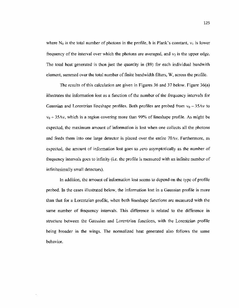
125

where No is the total number of photons in the profile, h is Plank's constant, vi is lower

frequency of the interval over which the photons are averaged, and v2 is the upper edge.

The totalheat generated is then just the quantity in (89) for each individual bandwith

element, summed over the total number of finite bandwidth filters, W, across the profile.

The results of this calculation are given in Figures 36 and 37 below. Figure 36(a)

illustrates the information lost as a function of the number of the frequency intervals for

Gaussian and Lorentzian lineshape profiles. Both profiles are probed from v<> - 35Av to

v0 + 35Av, which is a region covering more than 99% of lineshape profile. As might be

expected, the maximum amount of information is lost when one collects all the photons

and feeds them into one large detector is placed over the entire 70Av. Furthermore, as

expected, the amount of information lost goes to zero asymptotically as the number of

frequency intervals goes to infinity (i.e. the profile is measured with an infinite number of

infinitesimally small detectors).

In addition, the amount of information lost seems to depend on the type of profile

probed. In the cases illustrated below, the information lost in a Gaussian profile is more

than that for a Lorentzian profile, when both lineshape functions are measured with the

same number of frequency intervals. This difference is related to the difference in

structure between the Gaussian and Lorentzian functions, with the Lorentzian profile

being broader in the wings. The normalized heat generated also follows the same

behavior.

126

200

Fig. 36: (a) Information lost, in nats, plotted against the number of finite bandwidth intervals (N) needed to

cover the 70Av, for Gaussian and Lorentzian profiles. Note that the amount of information lost goes

asymptotically to zero, as the number of frequency intervals increases (equivalent to measuring with

infinitesimally sized detectors), (b) Heat generated when the lineshape profile is probed with finite

bandwidth frequency intervals. The total heat generated also goes asymptotically to zero, as the number of

frequency intervals increases. The heat generated, Q, is normalized to Q/N0h.

Figure 37 illustrates the relationship between the heat generated and the

information lost. Figure 37(a) shows the heat generated vs. the amount of information

lost. Consistent with the results of Bennet and others, the amount of heat generated

increases as the information lost increases. Also shown is the heat generated per bit lost

when the profile is measured with different numbers of frequency intervals of finite

bandwidths, in Figure 37(b). There appears to be a linear relationship between the heat

generated per bit lost and the number of frequency intervals used to probe the profile.

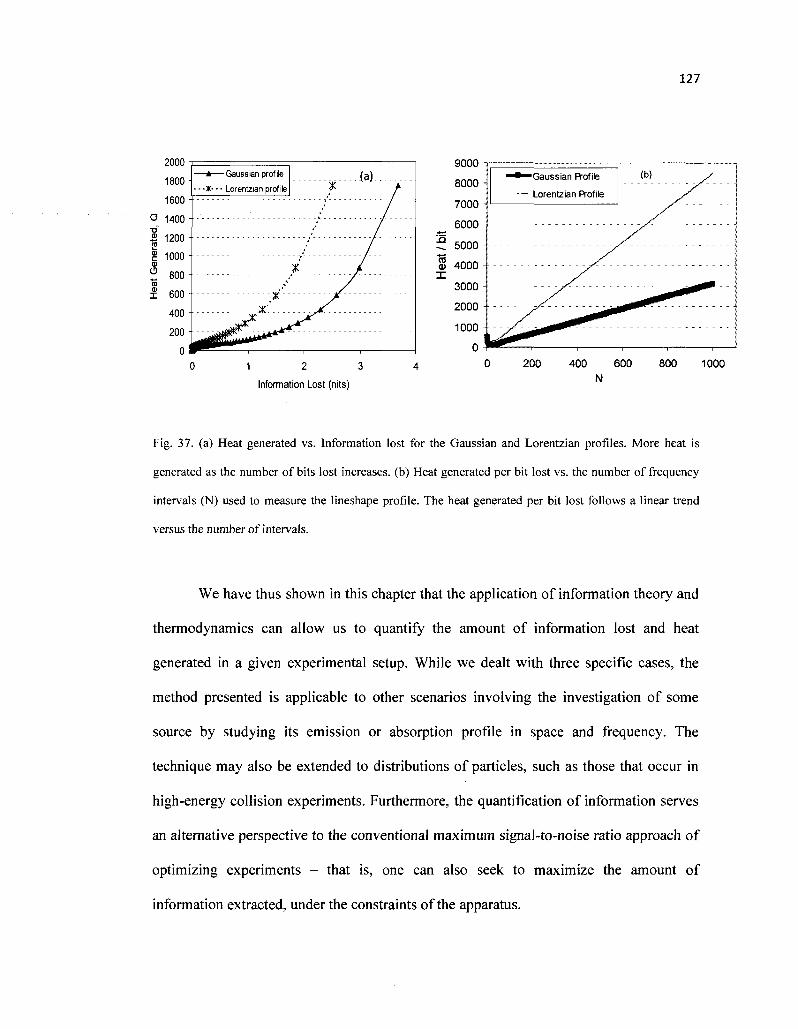
127

2000

1800

1600

0 1400

1 1200

2 1000

S 800

I 600

400

200

0

. : : — I

- - -X- • - Lorentzian profile

(a) *

/

* / /

x X"....

^gr ^

1 2 3

Information Lost (nits)

200 400 600 800 1000 N

Fig. 37. (a) Heat generated vs. Information lost for the Gaussian and Lorentzian profiles. More heat is

generated as the number of bits lost increases, (b) Heat generated per bit lost vs. the number of frequency

intervals (N) used to measure the lineshape profile. The heat generated per bit lost follows a linear trend

versus the number of intervals.

We have thus shown in this chapter that the application of information theory and

thermodynamics can allow us to quantify the amount of information lost and heat

generated in a given experimental setup. While we dealt with three specific cases, the

method presented is applicable to other scenarios involving the investigation of some

source by studying its emission or absorption profile in space and frequency. The

technique may also be extended to distributions of particles, such as those that occur in

high-energy collision experiments. Furthermore, the quantification of information serves

an alternative perspective to the conventional maximum signal-to-noise ratio approach of

optimizing experiments - that is, one can also seek to maximize the amount of

information extracted, under the constraints of the apparatus.

128

CHAPTER V. CONCLUSIONS

5.1 SUMMARY AND CONCLUSIONS

We developed and demonstrated the utility of a simultaneous higher order

harmonic detection system in the study of Oxygen A-band spectra. A system for the

collection of signals at multiple harmonics, simultaneously, was designed and

implemented using Labview. The results of the virtual lock-in amplifier developed were

compared to the sequential detection signals offered by a hardware based Stanford

Research Systems SR 850 lock-in amplifier, previously used by this research group. We

demonstrated that data collected by the two systems under identical experimental

conditions were within 5% of each other, which is within the experimental variations. By

doing so, we enhanced the experiment by first cutting the time required to run an

experiment by at least a factor of eight; and secondly, removing any susceptibility of the

experiment to changes in the environment that might occur on the time scale of collection

of data at each harmonic. For example, the ramp time in the experiments done in this

work was 40 seconds: it therefore takes at least 40 seconds to obtain each harmonic

signal. While this time scale is small in a laboratory environment, where there is a strong

attempt to control the experimental conditions, changes in the field can be more drastic.

Higher harmonic wavelength modulation spectroscopy signals were also used as a

powerful diagnostic tool for the comparison of lineshape functions. We presented

experimental results with theoretical comparisons probing multiple transitions in the

Oxygen A-band, simultaneously, to demonstrate the utility of wavelength modulation

spectroscopy in the investigation of gaseous behavior. In Chapter III, we examined the

129

sensitivity of higher harmonic signals to the form of the lineshape profile when modeling

under the same experimental parameters (temperature, pressure, etc). We illustrated that

the Voigt and Lorentzian absorption profiles have very similar structure at the

atmospheric conditions under which the experiments are run, and are therefore almost

indistinguishable when using conventional direct absorption spectroscopy. Higher

harmonic detection, however, showed greater sensitivity to the subtle differences between

the two lineshape functions, compared to lower order detection. The effects of increasing

modulation index on this ability to distinguish between profiles were also investigated. It

was shown that while a higher modulation index increased the magnitude of the signal,

the associated modulation broadening resulted in a loss of the finer structural differences

between the two profiles.

Another unique effect that we examined with wavelength modulation

spectroscopy was pathlength saturation: the non-uniform absorption across a profile over

long optical paths or high optical density. While such effects are commonly observed in

stellar and atmospheric spectra, where the absorption paths are several hundred to

thousands of kilometers, they are subtle with conventional direct absorption and lower

harmonic detection in the experimental environment where optical paths are on the order

of a few hundred meters. Higher harmonic signals, however, clearly illustrate this effect

as a depression of the peaks at linecenter, where absorption is greater than in the wings.

Furthermore, we showed that pathlength saturation effects provide an additional stringent

constraint when comparing models with different lineshape functions. For example,

under the same experimental parameters, the Lorentzian profile was unable to predict the

peak suppression that the model utilizing the Voigt profile did, when compared to the

130

experimental data. Wavelength Modulation Spectroscopy can therefore be used as a

diagnostic tool to distinguish between two different lineshape functions, in an

environment where conventional direct absorption spectroscopy is not a sufficiently

sensitive probe for the purpose. This allows for the more accurate characterization of

gaseous parameters and their molecular behavior.

We also presented, in Chapter III, the application of wavelength modulation

spectroscopy for the detection of weak spectra. The region we probed has been well

documented with other spectroscopic methods to contain at least eight optical transitions

[39]. Most of these transitions were isotopic counterparts of the two transitions probed in

the section 3.2. While those two, the RR(13,13) and RQ(11,12), are already many orders

of magnitude weaker than common electric dipole driven transitions, the isotopic

transitions are a further 100 times weaker due to the much lower atmospheric

concentrations. As a result, these weaker transitions are "hidden" under the wings of

stronger surrounding lines, and were unresolved with direct absorption spectroscopy. The

very subtle features of these additional spectra, however, which were indiscernible with

direct absorption and lower harmonic detection, were amplified at higher detection

orders. The impact of increasing modulation index on the resolution ability of WMS

signals was also investigated. Again, the resulting modulation broadening was found to

reduce the ability to discern the weak spectra lines. In general, however, higher harmonic

wavelength modulation spectroscopy signals provide the ability to examine weak spectra

that are otherwise difficult to detect under given experimental resolutions.

Both these applications arise due to the derivative-like behavior of WMS higher

order signals, which in general have N zero crossings and N+l turning points. Since the

131

N-th harmonic signal has the structure of the N-th derivative of the direct absorption

signal, any small features (that may not be discernible depending on the resolutions

available) are amplified. Our experiments also show that the additional structure imposed

on the usual WMS signals because of pathlength saturation can be an important aid to

drawing conclusions regarding internal gaseous molecular dynamics.

In Chapter IV, we introduced a novel aspect of looking at absorption signals. We

discussed the quantification of information that one obtains when determining parameters

from a distribution of photons, in either space or frequency. Principles of Shannon's

information theory were applied to calculate the information that one obtains from

measurements of antenna array radiation patterns, which are spatial photon distributions.

We investigated the information gained when one is attempting to determine the inter-

element phase from the location of turning points in the radiation pattern, under finite

spatial detector resolution. We found that for a given spatial extent of the detector, the

more sensitive turning points gave the most amount of information about changes in the

inter-element phase. In addition, the technique was general and applicable to the

measurement of other parameters of the array. We also calculated, using the same

methodology, the information gained from WMS signals about linewidth measurements

at higher detection orders. We found that higher sensitivity of higher detection order

signals, demonstrated experimentally in Chapter III, was associated with a larger amount

of information gained with respect to the direct absorption signals.

Last, but not least, we calculated the information lost and heat generated when a

direct absorption lineshape profile is measured with a finite resolution spectrometer. It

was shown that there is a finite amount of information that one can obtain from such an

132

experiment, and an associated amount of heat generated when part of that information is

lost. Such calculations form the foundation of future work in optimization of experiments

for the maximum extraction of information, compared to the conventional methods of

increasing signal to noise ratio. For example, while our WMS signals had decreasing

amplitude with increasing detection order, and therefore a lower signal-to-noise ratio, the

greater amount of structure offered by higher harmonics provided more information

about linewidth structure and weak spectra.

5.2 FUTURE WORK

Wavelength modulation spectroscopy has many more applications, in addition to

those discussed in this work. For instance, while the technique was utilized to investigate

two specific lineshape functions, namely the Lorentzian profile and the Voigt profile, the

methods presented were general and may be extended, under sufficient experimental

accuracy, to other lineshape functions (e.g. Rautian-Sobel'man, Galatry, etc.).

Furthermore, the same techniques could be applied to perform detection of possible

subtle features such as Dicke narrowing.

In addition, WMS might also be applicable in future studies of stellar

atmospheres, where pathlength saturation is a common occurrence. The absorption and

emission features from many stars are naturally modulated - for example because of

stellar wobble resulting from orbiting planets [67]. WMS techniques could be applied on

these modulated stellar spectra to resolve subtle features that may not be as obvious with

conventional spectroscopic methods. Another extension of our work is wavelength

133

modulation spectroscopy of emission profiles, for applications in environments where we

may be unable to send a probe beam.

Another application of higher harmonic signals is in the frequency stabilization of

lasers [68]. The zero crossing at linecenter of odd harmonics provides us with a

correction signal if a laser were to drift away from this center. Furthermore, the derivative

structure at higher harmonics results in steeper slopes around the zero crossings at odd

harmonics. Hence, while the amplitude and range of the correction signal may be smaller

at higher harmonics, the larger slope would allow for a tighter lock on the laser. This is

where simultaneous harmonic detection would be very useful, where one can determine a

correction signal from the multiple harmonic signals.

In conclusion, we have demonstrated the utility of a simultaneous multiple

harmonics wavelength modulation spectroscopy system in the precise characterization of

lineshape profiles and the detection of weak spectra, as well as pathlength saturation

effects. We have also presented a novel method of applying Shannon's information

theory principles to quantifying the information in WMS signals.

134

BIBLIOGRAPHY

1. K. D. Mohan, M. A. Khan, A. N. Dharamsi, Proc. SPIE 7310, DOI: 10.1117/12.818574 (2009).

2. A. N. Dharamsi, Y. Lu, Appl. Phys. B 62, 273 (1996). 3. A. N. Dharamsi, A. M. Bullock, Appl. Phys. B 63, 283 (1996). 4. A. M. Bullock, A. N. Dharamsi, W. P. Chu, L. R. Poole, Appl. Phys. Lett. 70,1195 (1997). 5. M. A. Khan, K. Mohan, A. N. Dharamsi, Appl. Phys. B 99, 363 (2010). 6. A. N. Dharamsi, J. Phys. D 29, 540 (1996). 7. A. M. Bullock, A. N. Dharamsi, J. Appl. Phys. 84, 6929 (1998). 8. S. Schilt, L. Thevenaz, P. Robert, Appl. Opt. 42, 6728 (2003). 9. A. Farooq, J. B. Jeffries, R. K. Hanson, Appl. Phys. B 96,161 (2009). 10. G. B. Rieker, J. B. Jeffries, R. K. Hanson, Appl. Phys. B 94, 51 (2009). 11. L. Ciaffoni, B.L Cummings, W. Denzer, R. Peverall, S.R. Procter, G.A.D. Ritchie, Appl.

Phys. B 92, 627 (2008). 12. C. E. Shannon, Bell System Tech. J. 27, 379 (1948). 13. C. E. Shannon, Bell System Tech. J. 27, 623 (1948). 14. K. D. Mohan, M. A. Khan, A. N. Dharamsi, Proc. SPIE 6377, DOI: 10.1117/12.685219

(2006). 15. K. D. Mohan, M. A. Khan, A. N. Dharamsi, Proc. SPIE 6008, DOI: 10.1117/12.629792

(2005). 16. K. D. Mohan, M. A. Khan, A. N. Dharamsi, Proc. SPIE 6299, DOI: 10.1117/12.679522

(2006). 17. M. A. Khan, K. D. Mohan, A. N. Dharamsi, in Frontiers in Optics, OSA Technical Digest

Series (Optical Society of America, 2005), paper FTuT5. 18. M. A. Khan, K. D. Mohan, A. N. Dharamsi, in Frontiers in Optics, OSA Technical Digest

(CD) (Optical Society of America, 2008), paper FWI4. 19. K. D. Mohan, M. A. Khan, A. N. Dharamsi, Manuscript Submitted to Applied Physics B,

April 2010. 20. M. C. Pitts, L W. Thomason, W. P. Chu, "Satellite Remote Sensing of Temperature and

Pressure by the Stratospheric Aerosol and Gas Experiment III" <http://www-sage3.larc.nasa.gov/library/media/ams satellite.pdf> Last Accessed March 18, 2010.

21. C. T. McElroy, C. R. Nowlan, J. R. Drummond, P. F. Bernath, D. V. Barton, D. G. Dufour, C. Midwinter, R. B. Hall, A. Ogyu, A. Ullberg, D. I. Wardle, J. Kar, J. Zou, F. Nichitiu, C. D. Boone, K. A. Walker, N. Rowlands, Appl. Opt. 46,4341 (2007).

22. R. S. Mulliken, Phys. Rev. 32, 880 (1928). 23. G. H. Dieke, H. D. Babcock, Proc. Nat. Acad. Sci. 13, 670 (1927). 24. J. Altman, R. Baumgart, C. Weitkamp, Appl. Opt. 20, 995 (1981). 25. G. Fowles, Modern Optics, Second ed. (Dover Publications Inc, New York, New York,

1989). 26. D. Bohm, Quantum Theory. (Prentice Hall Inc, Englewood Cliffs, New Jersey, 1951). 27. R. White, Basic Quantum Mechanics. (McGraw-Hill Inc, New York, New York, 1966). 28. J. D. Jackson, Classical Electrodymanics, Second Edition. (John Wiley & Sons Inc, New

York, New York, 1975). 29. J. T. Verdeyen, Laser Electronics. (Prentice Hall Inc, Upper Saddle River, New Jersey,

2000).

135

30. H. A. Bethe, E. E. Salpeter, Quantum Mechanics of One-And-Electron Atoms. (Plenum Publishing Corp., New York, New York, 1977).

31. A. N. Cox, Allen's Astrophysical Quantities, Fourth Edition. (Springer-Verlag Inc, New York, New York, 2000).

32. A. Einstein, Doc. 34 The Collected Papers of Albert Einstein, Volume 6: The Berlin Years: Writings, 1914-1917. Edited by A. J. Kox, M. J. Klein and R. Schulmann (Princeton University Press 1996).

33. R. S. Mulliken, Rev. Mod. Phys. 2, 60 (1930). 34. R. S. Mulliken, Rev. Mod. Phys. 3, 89 (1931). 35. R. S. Mulliken, Rev. Mod. Phys. 4 , 1 (1932). 36. G. Herzberg, Molecular Spectra and Molecular Structure I. Spectra of Diatomic

Moleculaes, Second Edition. (D. Van Nostrand Company Inc, Princeton, New Jersey, 1959).

37. H. Haken, H. C. Wolf, Molecular Physics and Elements of Quantum Chemistry, Second Edition. (Springer-Verlag, Berlin, Germany, 2004).

38. P. Atkins, J. de Paula, R. Friedman, Quanta, Matter and Change. (W. H. Freeman & Company, New York, New York, 2009).

39. L. S. Rothman, I. E. Gordon, A. Barbe, D. ChrisBenner, P. F. Bernath, M. Birk, V. Boudon, L. R. Brown, A. Campargue, J. -P. Champion, K. Chance, L. H. Coudert, V. Dana, V. M. Devi, S. Fally, J. -M. Flaud, R. R. Gamache, A. Goldman, D. Jacquemart, I. Kleiner, N. Lacome, W. J. Lafferty, J. -Y. Mandin, S. T. Massie, S. N. Mikhailenko, C. E. Miller, N. Moazzen-Ahmadi, O. V. Naumenko, A. V. Nikitin, J. Orphal, V. I. Perevalov, A. Perrin, A. Predoi-Cross, C. P. Rinsland, M. Rotger, M. Simeckova, M. A. H Smith, K. Sung, S. A. Tashkun, J. Tennyson, R. A. Toth, A. C. Vandaele, J. VanderAuwera, J. Quant. Spectrosc. Radiat. Transfer 110, 533 (2008).

40. M. G. Littman, H. J. Metcalf, Appl. Opt. 17, 2224 (1978). 41 . S. F. Yu, Analysis and Design of Vertical Cavity Surface Emitting Lasers. (John Wiley &

Sons Inc, Hoboken, New Jersey, 2003). 42. M. Orentstein, A. C. Von Lehmen, C. Chang-Hasnain, N. G. Stoffel, J. P Harbison, L. T.

Florez, Electron. Lett. 27, 437 (1991). 43. J. Reid, D. Labrie, Appl. Phys. B 26, 203 (1981). 44. G. V. H. Wilson, J. Appl. Phys. 34, 3276 (1963). 45. O. E. Myers, E. J. Putzer, J. Appl. Phys. 30,1987 (1959). 46. L H. Aller, Atoms, Stars, and Nebulae. (Harvard University Press, Cambridge,

Massachusetts, 1971). 47. M. A. Khan, K. D. Mohan, A. N. Dharamsi, Proc. SPIE 6378, DOI: 10.1117/12.685642

(2006). 48. L.R. Carlson, S.A. Johnson, E.F. Worden, C.A. May, R.W. Solarz, J.A. Paisner, Optics

Communications 21,116 (1977). 49. L. Galatry, Phys. Rev. 122,1218 (1961). 50. S. G. Rautian, 1.1. Sobel'man, Soviet Physics Uspekhi 9, 701 (1967). 51. P. R. Berman, J. Quant. Spectrosc. Radiat. Transfer 12,1331 (1972). 52. R. G. Breene, Rev. Mod. Phys. 29, 94 (1957). 53. H. Margenau, W. W. Watson, Rev. Mod. Phys. 8, 22 (1936). 54. R. H. Dicke, Phys. Rev. 89, 472 (1953). 55. K. J. Ritter, T. D. Wilkerson, J. Mol. Spectrosc. 1 2 1 , 1 (1987). 56. P. L Varghese, R. K. Hanson, Appl. Opt. 23, 2376 (1984).

136

57. E. B. Jenkins, Phys. Scr. 2009 014005, DOI: 10.1088/0031-8949/2009/T134/014005 (2009).

58. E. T. Jaynes, Proc. IEEE 70, 939 (1982). 59. E. T. Jaynes, Probability Theory : the logic of science. (Cambridge University Press, New

York, New York, 2005). 60. R. C. Tolman, The Principles of Statistical Mechanics. (Dover Publications, New York,

New York, 1979). 61. J. C. Maxwell, Scientific papers; edited by William Davidson Niven. (Dover Publications,

New York, New York, 1952). 62. R. Landauer, IBM J. Research and Development 5, 261 (1961). 63. C. H. Bennet, Intl. J. Theoretical Phys. 21, 905. 64. P. F. McManamon, T. A. Dorschner, D. L. Corkum, L. J. Friedman, D. S. Hobbs, M. Holz, S.

Liberman, H. Q. Nguyen, D. P. Resler, R. C. Sharp, E. A. Watson, Proc. IEEE 84, 268 (1996).

65. D. P. Resler, D. S. Hobbs, R. C. Sharp, L. J. Friedman, T. A. Dorschner, Opt. Lett. 21, 689 (1996).

66. A. Einstein, Doc. 26, The Collected Papers of Albert Einstein, Volume 6: The Berlin Years: Writings, 1914-1917. (English translation supplement). Translated by Alfred Engel, Edited by A. J. Kox, M. J. Klein, and R. Schulmann (Princeton University Press, Princeton, New Jersey 1997).

67. T. Takeuchi, T. Velusamy, D. N. C. Lin, Astroph. J. 618, 987 (2005). 68. G. J. Koch, A. N. Dharamsi, C. M. Fitzgerald, J. C. McCarthy, Appl. Opt. 39 (2000).

137

APPENDIX A:

VIRTUAL LOCK-IN AMPLIFIER PROGRAM IMPLEMENTED IN LAB

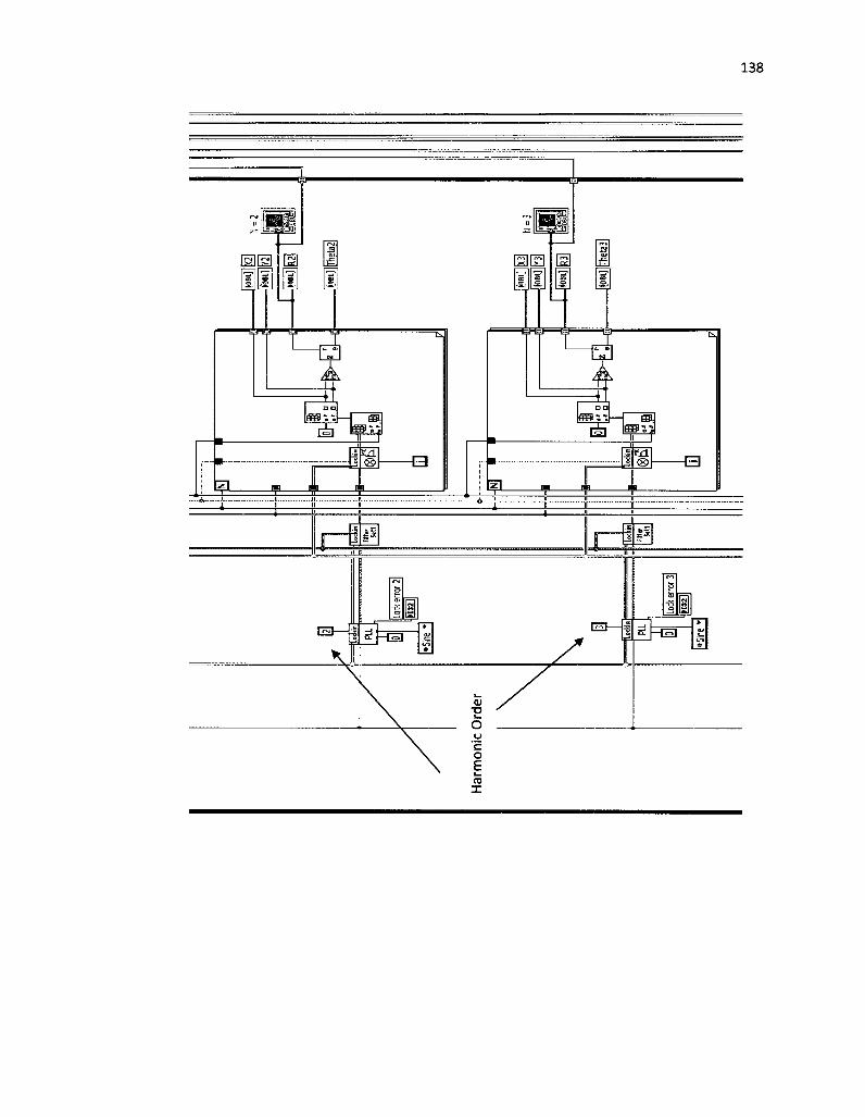
Har

mo

nic

Ord

er

m\

w rt

0-

d]

ET

? •cck

lw

•HJ

%i#

>-H

-J

NT

E

JWllT

lieta

2|

Mi

N =

3

-Lfw

liU

JtPB

t] ||T

heta

3|

00

APPENDIX B:

MATLAB PROGRAM USED FOR MODELING WMS SIGNALS

%This program models for 5 lines, with amplitude modulation, including pathlength saturation effect

format long;

dnucl = 1.15*2*0.0458*3el0*le-9: dnuc2 = 1.15*2*0.0468*3el0*le-9 dnuc3 = 1.10*2*0.0468*3el0*le-9 dnuc4= 1.10*2*0.0463*3el0*le-9 dnuc5 = 1.00*2*0.0458*3el0*le-9

%colHsion broadened FULL WIDTH half max GHz from hitran %collision broadened FULL WIDTH half max GHz from hitran %collision broadened FULL WIDTH half max GHz from hitran %collision broadened FULL WIDTH half max GHz from hitran %collision broadened FULL WIDTH half max GHz from hitran

f01cm=13151.34866; %line center of line in cm-1, from hitran f02cm=13150.19663; %line centerof line in cm-1, from hitran f03cm=13150.75594; %line center of line in cm-1, from hitran f04cm=13150.26139; %line centerof line in cm-1, from hitran f05cm=13151.73584; %line centerof line in cm-1, from hitran

c0=3e8; %speed of light in m/s cl=3el0; %speed of light in cm/s f01=f01cm*cl*le-9; %line center 1 in GHz f02=f02cm*cl*le-9; %line center 2 in GHz f03=f03cm*cl*le-9; %line center 3 in GHz f04=f04cm*cl*le-9; %line center 4 in GHz f05=f05cm*cl*le-9; %line center 5 in GHz 101=(l/f01cm)*(le-2)*le6; %line center 1 in microns 102=(l/fD2cm)*(le-2)*le6; %line center 2 in microns 103=(l/f03cm)*(le-2)*le6; %line center 3 in microns 104=(l/f04cm)*(le-2)*le6; %line center 4 in microns 105=(l/f05cm)*(le-2)*le6; %line center 4 in microns

%Assuming doppler width same on both lines T=296; %room temperature in Kelvin k=1.3806503e-23; %Boltzmann Constant m0=2*16*1.66e-27; %mass of oxygen molecule in kg

%First line's doppler width dnudl = f01*sqrt((8*k*T*log(2))/(mO.*(cO.A2)));%doppler linewidth GHz, estimated from temperature and

mass dnudbarl = dnudl/(sqrt(4*log(2))); %modified (normalized) doppler linewidth bl=dnucl/(2*dnudbarl); %voigt parameter

%Second line's doppler width dnud2 = fD2*sqrt((8*k*T*log(2))/(mO.*(cO.A2)));%doppler linewidth GHz, estimated from temperature and

mass dnudbar2 = dnud2/(sqrt(4*log(2))); %modified (normalized) doppler linewidth b2=dnuc2/(2*dnudbar2); %voigt parameter

%Third line's doppler width

140

dnud3 = f03*sqrt((8*k*T*log(2))/(mO.*(cO.A2)));%doppler linewidth GHz, estimated from temperature and mass

dnudbar3 = dnud3/(sqrt(4*log(2))); %modified (normalized) doppler linewidth b3=dnuc3/(2*dnudbar3); %voigt parameter

%Fourth line's doppler width dnud4 = f04*sqrt((8*k*T*log(2))/(mO.*(cO.A2)));%doppler linewidth GHz, estimated from temperature and

mass dnudbar4 = dnud4/(sqrt(4*log(2))); %modified (normalized) doppler linewidth b4=dnuc4/(2*dnudbar2); %voigt parameter

%Fifth line's doppler width dnud5 = f05*sqrt((8*k*T*log(2))/(mO.*(cO.A2))); %doppler linewidth GHz, estimated from temperature

and mass dnudbar5 = dnud5/(sqrt(4*log(2))); %modified (normalized) doppler linewidth b5=dnuc5/(2*dnudbar5); %voigt parameter

%gas parameters for main lines (first 2 - 0 - 1 6 ) nd = (0.20946*101325*0.99)/(k*T)*(0.01A3);%gas density /cm3 L = (2*131.4*46)+(2*25);%path length cm sigmal = 5.62E-24*3el0*le-9; %cross section cm2-GHz line 1 sigma2 = 7.63E-24*3el0*le-9; %cross section cm2-GHz line 2 al=nd*sigmal*L; a2=nd*sigma2*L; g01=(bl-*exp(blA2).*erfc(bl))/(sqrt(pi)*(dnucl/2)); g02=(b2.*exp(b2A2).*erfc(b2))/(sqrt(pi)*(dnuc2/2));

%gas parameters for weak lines (second 2 - O-l 8) nd = (0.20946*101325*0.00201)/(k*T)*(0.01A3);%gas density /cm3 L = (2*131.4*46)+(2*25);%path length cm sigma3 = l/0.00201*1.54E-26*3el0*le-9; %l/0.00201*cross section cm2-GHz line 3 sigma4 = l/0.00201*1.27E-26*3el0*le-9; %l/0.00201*cross section cm2-GHz line 4 sigma5 = 1/0.00201*1.16E-26*3elO*le-9; %l/0.00201*cross section cm2-GHz line 5 a3=nd*sigma3*L; a4=nd*sigma4*L; a5=nd*sigma5*L; g03=(b3.*exp(b3A2).*erfc(b3))/(sqrt(pi)*(dnuc3/2)); g04=(b4.*exp(b4A2).*erfc(b4))/(sqrt(pi)*(dnuc4/2)); g05=(b5.*exp(b5A2).*erfc(b5))/(sqrt(pi)*(dnuc5/2));

%modulation voltage beta = 0.0056*c0/((((101+102)/2)*le-6)A2)*0.0017e-6*le-9; %swing in frequency GHz ml = betaZ(dnudbarl); %modulation index line 1 m2 = beta/(dnudbar2); %modulation index line 2 m3 = beta/(dnudbar3); %modulation index line 3 m4 = beta/(dnudbar4); %modulation index line 4 m5 = beta/(dnudbar5); %modulation index line 5

v=le-9*c0./(lambda*le-6); %frequencies from wavelength points in GHz r=1.31e-5; %amplitude modulation index psi=pi; rho=-2.533887e-6; %ramp index 10=1;

141

theta=-pi:0.0001:pi; dtheta=theta(2)-theta( 1);

for N=8:1:8 %N=Harmonic Order for i=l:size(v); - N

forj=l:size(theta,2); SlG)=quad(@voigtweakQuad,-10,10,10A-8,[],v(i),bl,beta,dnucl/2,fDl,al,theta(j)); S2G)=quad(@voigtweakQuad,-10,10,10A-8,[],v(i),b2,beta,dnuc2/2,fD2,a2,thetaG)); S30)=quad(@voigtweakQuad,-10,10,10A-8,[],v(i),b3,beta,dnuc3/2,f03,a3,thetaG)); S4G)=quad(@voigtweakQuad,-10,10,10A-8,[],v(i),b4,beta,dnuc4/2,f04,a4,thetaG)); S5G)=quad(@voigtweakQuad,-10,10,10A-8,[],v(i),b5,beta,dnuc5/2,fD5,a5,thetaG));

end S(i,N)=sum(cos(N.*theta).*I0.*(l+(rho.*v(i))+(r.*cos(theta+psi))).*exp(Sl+S2+S3+S4+S5).*dtheta);

%rectangular integration end

end

RS=abs(S); figure plot(lambda,RS);

142

VITA

Karan D. Mohan

EDUCATION Old Dominion University (ODU), Norfolk, VA Doctor of Philosophy, Electrical Engineering, GPA: 4.00/4.00, August 2010 Master of Engineering, Electrical Engineering, GPA: 4.00/4.00, August 2008 Bachelor of Science, Electrical Engineering (Minor in Physics), GPA: 3.94/4.00, May 2004

EXPERIENCE Research Assistant, Laser & Plasma Engineering Institute at ODU; 04/2004 - Present • Performed theoretical and experimental research synthesizing areas in Lasers; Spectroscopy;

Antenna Arrays; Electromagnetics and Optics; Remote Sensing; Statistics; Information Theory. • Responsible for design, collection, analysis, modeling and documentation of procedures and data

from experiments involving sensing of various atmospheric oxygen parameters. • Developed new detection techniques in Wavelength Modulation Spectroscopy, as well as a new

metric of measurement quality utilizing Information Theory. • Presented and published results in journals and national conferences.

Research Assistant, Laser & Plasma Engineering Institute at ODU; 01/2003 - 04/2004 • Performed theoretical research, studying Quantum Mechanics of optically induced transitions in

atoms and molecules. • Programmed Mathematica scripts to analyze the properties of hydrogen atom transitions. • Presented novel results at national conferences, of optical transitions in the hydrogen atom.

Research Assistant, Department of Physics at ODU; 01/2002 - 05/2002 • Performed theoretical and experimental research in the Atomic, Molecular and Cold Physics Lab, for

Laser Cooling/Trapping project, developing a Permanent Magnet Zeeman Slower. • Developed C++ code to simulate magnetic fields of various permanent magnet configurations, as

well as performed experimental measurements of fields in the configurations.

Instructor; Depts. of ECE, Mathematics, and General Education; 09/2002 - Present • Responsible for complete organization, preparation, and delivery of various classes with up to 100+

students.

JOURNAL PUBLICATIONS 1) M. Amir Khan, K. Mohan, A.N. Dharamsi, "Optical Pathlength Saturation signatures in

wavelength modulation spectroscopy signals of atmospheric molecular oxygen," Applied Physics B: Lasers and Optics, 99, 363 (2010)

2) K. D. Mohan, M. Amir Khan, A.N. Dharamsi, "Characterization of Lineshape Structure by Wavelength Modulation Spectroscopy," Submitted to Applied Physics B: Lasers and Optics, April 2010.

CONFERENCE PROCEEDINGS AND PRESENTATIONS

1) Karan D. Mohan, Mohammad A. Khan, Amin N. Dharamsi, "Optimization of nano-photonic sensors and detectors by information theoretic principles," Proceedings of SPIE: Vol 6008 --Nanosensing Materials and Devices II, (November 2005)

143

2) Karan D. Mohan, Mohammad A. Khan and Amin N. Dharamsi , "Minimum harmonic detection order for Rayleigh resolution in modulation spectroscopy," Proceedings of SPIE: VoL 6299 — Remote Sensing of Aerosol and Chemical Gases, Model Simulation/Assimilation, and Applications to Air Quality, (September 2006)

3) K. Mohan, M. Khan and A. Dharamsi, "Thermodynamics of information loss in spectroscopic measurements," Proceedings of SPIE: VoL 6377 — Advanced Environmental, Chemical, and Biological Sensing Technologies IV, (October 2006)

4) Karan Mohan, M. Amir Khan, Amin Dharamsi, "Information Content in Antenna Radiation Patterns," presented at 75th Annual Meeting of the Southeastern Section of APS, (October 2008)

5) Karan D. Mohan, M. Amir Khan and Amin N. Dharamsi, "A Quantitative Measure for Information Content in Antenna Array Radiation Patterns," Proceedings of SPIE: VoL 7310 — Non-Intrusive Inspection Technologies II, (April 2009)

6) M. A. Khan, K. D. Mohan, and A. N. Dharamsi, "Thermodynamic Efficiency of Information Processing in Photonic Devices," Frontiers in Optics, OSA Technical Digest Series (Optical Society of America), (October 2005)

7) M. A. Khan, K. D. Mohan and A. N. Dharamsi, "Novel pathlength saturation effects in modulation spectroscopic techniques," Proceedings of SPIE: VoL 6378 — Chemical and Biological Sensors for Industrial and Environmental Monitoring II, (October 2006)

8) M. A. Khan, K. D. Mohan, and A. N. Dharamsi, "Information Theory of High-Precision Measurements," Frontiers in Optics, OSA Technical Digest (CD) (Optical Society of America), (October 2008)

9) M. Amir Khan, Karan D. Mohan, A.N. Dharamsi, "Information Extraction from Congested Molecular Spectra by Modulation Spectroscopy" Presented at 75th Annual Meeting of the Southeastern Section of APS, (October 2008)

10) M. A. Khan, K. D. Mohan, and A. N. Dharamsi, "Signal Structure and Precision in Optical Measurements: A new perspective to optimal experimental techniques," 21st Annual Meeting of the IEEE Lasers and Electro-Optics Society, 2008. LEOS 2008, (November 2008)

11) M. Amir Khan, Karan D. Mohan, A. N. Dharamsi, "Signal Structure and Sensitive Detection of Molecular Species: Optimal experimental techniques in Modulation Broadened Wavelength Modulation Spectroscopy," Proceedings of SPIE: VoL 7229 — Vertical-Cavity Surface-Emitting Lasers XIII, (February 2009)

AWARDS / HONORS • Newport and Spectra-Physics Research Excellence Award • University-wide Teaching Assistantship • Stuart Russell Scholarship • Faculty Award for Academic Achievement in Electrical Engineering • Office of International Programs Academic Achievement Award • Education Foundation of the Engineer's Club of Hampton Roads Scholarship • Charles H. Eure Memorial Scholarship • Academic Honors Scholarship • International Student Scholarship