Secular stagnation in Belgium? - serv.be · Secular stagnation in Belgium? ... As we saw in the...

Secular stagnation in Belgium?– determinants and policy recommendations –

Freddy Heylen

- Ghent University -

SERVacademie: The future of productivity

23 September 2016

- Finale versie van deze presentatie 26/9/2016 -

Figure 1a. Growth rate of real GDP per capita (Belgium, annual averages, in %)

Data source: Penn World Tables 8.1.

For 2011-2020 Federal Planning Bureau (Economische Vooruitzichten MLT, 2016-21).

Introduction and research questions

2

0,0

1,0

2,0

3,0

4,0

5,0

1951-60 1961-70 1971-80 1981-90 1991-00 2001-10 2011-20

3

Figure 1.b. Ten-year real government Real long-term corporate bond

bond yields (1980-2015, in %) yield (US, 1981-2015, in %)

Source: King and Low (2014) and Rachel and Smith (2015).

0,0

3,0

6,0

9,0

12,0

1981 1986 1991 1996 2001 2006 2011

Real corporate bond yield, in %, US

Source: Moody’s (nominal corporate bond rate BAA)

and Philadelphia FED (10-year ahead inflation

forecasts)


Have OECD countries entered a very long period of low

economic growth and rock-bottom real interest rates… a

secular stagnation?

4

Some economist say yes (Krugman, 2014; Summers, 2014, 2015; Buiter et al., 2015).


Other economists say no (Goodhart & Erfurth, 2014; Mokyr, 2014; Bernanke, 2015;

Rogoff, 2015; …).

A clear opposition in views… � Our research questions:

Secular stagnation: could it be possible?

And what would be the main driving forces?

What are the policy implications and recommendations?

Overview of the presentation

0. Introduction and research questions

1. Literature on secular stagnation: driving forces

- Slowdown in technical progress?

- Demographic change

- Rising inequality

- Other (deleveraging after financial crisis, fiscal consolidation, a lower bound to the interest rate,…)

2. A general equilibrium analysis (OLG model)

3. Model simulations

4. Conclusions, policy implications and recommendations

5F. Heylen, UGent, 26 September 2016

Driving forces of secular stagnation:

Slowdown in technical progress?

• In the very long run, per capita growth is equal to the rate of technical progress.

• Consider a neoclassical production function,

The long-run per capita growth rate is

The last decades show a strong decline in x.

Note: TFP-growth = (1-α-γ)x. We impose in our model α=0,255 and γ=0,12 => TFP-growth = 0,625 x

= effective labour (rising in number of employed workers L,

and in workers’ ability and human capital h)

Kt = private physical capital, Gt = public capital

7

Average annual rate of technical change (x) in %

1950-2009 : actual data

2010-... : our projection.



0,0

1,0

2,0

3,0

4,0

1950-64 1965-79 1980-94 1995-2009 2010-24 2025-39 2040-54 2055-69

Annual rate of technical change (x) Annual per capita GDP growth



• In the very long run, per capita growth is equal to the rate of technical progress.

• Consider a neoclassical production function,

The long-run per capita growth rate is

The last decades show a strong decline in x. What about the future?

Optimists (Mokyr, 2014) and ‘realists’ (Gordon, 2014, 2015; Fernald and Jones,

2014; IMF, 2015).

Our assumption/projection...

9

Average annual rate of technical change (x) in %

1950-2009 : actual data

2010-... : our projection. Motivation? AWG, Gordon (2014)



0,0

1,0

2,0

3,0

4,0

1950-64 1965-79 1980-94 1995-2009 2010-24 2025-39 2040-54 2055-69

Annual rate of technical change (x) Annual per capita GDP growth

Annual rate of technical progress (in %, *)

EU AWG EU AWG-risk Our

2010-24 0,6 0,6 0,6

2025-39 1,3 1,1 1,1

Long-run 1,5 1,25 1,25

• In the long run, per capita growth equals the rate of technical progress (x).

• In the intermediate period, per capita growth may be different. Demography!

• Arithmetically: lower per capita growth when total population grows faster

than employment

• Demographic change affects the behaviour of households and firms, i.e.

labour supply and demand, schooling, investment in physical capital.

10

Negative effect from

rising dependency

rate

Positive effect from

rising employment

rate


Demographic change

Note: nPOPgrowth rate of total population; nN growth rate of population at working age;

nL : growth rate of employment

40

50

60

70

80

1950 1960 1970 1980 1990 2000 2010 2020 2030 2040 2050 2060

Age dependency ratio, in % (-15 and +64 versus 15-64)

11

Overall dependency ratio (Belgium, in %)

Sources: OECD Historical population data and projections;

Belgian Federal Planning bureau and FOD Economie (ADS), Bevolkingsvooruitzichten 2015-2060 (maart 2016).

1 2 3 4 1, 4 : demography

weighs negatively on

per capita growth

2: demography raises

per capita growth


Demographic change

12

Growth effects of projected demographic change – for unchanged

employment rate (Belgium)

Average annual growth rate of population at working age relative to total population

(nN – nPOP, in %-points).

Sources: see previous slide

1951-61 1961-70 1971-80 1981-90 1991-00 2001-10 2011-20 2021-30 2031-40 2041-50 2051-60


Demographic change

-0,60

-0,45

-0,30

-0,15

0,00

0,15

0,30

0,45

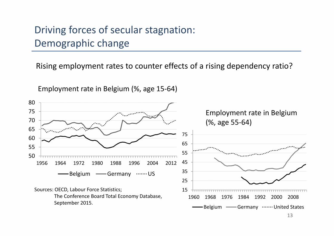
13

Employment rate in Belgium (%, age 15-64)

Sources: OECD, Labour Force Statistics;

The Conference Board Total Economy Database,

September 2015.

50

55

60

65

70

75

80

1956 1964 1972 1980 1988 1996 2004 2012

Belgium Germany US

15

25

35

45

55

65

75

1960 1968 1976 1984 1992 2000 2008

Belgium Germany United States

Employment rate in Belgium

(%, age 55-64)

Rising employment rates to counter effects of a rising dependency ratio?


Demographic change

14

Rising employment rates to counter effects of a rising dependency ratio?

Source: OECD Labour Force Statistics; for 2011-2020 Federal Planning Bureau (Economische Vooruitzichten

MLT, 2016-21, juni 2016).

Average annual growth rate of the employment rate

(nL – nN, in %-points)

-1,0

-0,5

0,0

0,5

1,0

1,5

1951-60 1961-70 1971-80 1981-90 1991-00 2001-10 2011-20


Demographic change

• In the long run, per capita growth equals the rate of technical progress.

• In the intermediate period, per capita growth may be different:

• Demographic arithmetic:

• Demographic change may affect behaviour of households and firms: labour

supply and demand (L), investment rates in physical capital (K), investment

in education (h).

Source of weak growth and stagnation? (arguments, counterarguments)

15


Demographic change

Behavioural effects of demographic change source of weak growth and stagnation?

• Decline in working age population � fall in the productivity of physical capital and

reduced need for capital � less investment (Ludwig et al., 2012; Heylen and Van de Kerckhove,

2013; Summers, 2014)

• Counterargument: the end of cheap labour � reduction of relative cost of capital �

more investment (Goodhart and Erfurth, 2014)

• Increasing longevity � work longer, increased saving during active life (Krueger and Ludwig)

� perspective of longer working life promotes education when

young (Ben-Porath, 1967; …)

� availability of more and better educated workers � higher

productivity of physical capital � more investment

• Increasing longevity � young retirees save more (Onder and Pestieau, 2014)

• Counterargument : lifecycle theory: (a growing group of) older retirees dissave

• Rising savings may feed through into lower interest rates � promote investment 16


Demographic change

17


Rising inequality

18


Rising inequality

19

Sources of rising inequality?

• Inequality in financial wealth, income from wealth and wealth transfers (e.g. bequests)

(Piketty, 2014)... (Note: Secular stagnation could further raise inequality).

• Inequality in human capital and the return to human capital

(Kanbur and Stiglitz, 2015)

• Counterargument:

• Higher inequality = higher reward for effort and success, for schooling � positive for

investment


Rising inequality

Growing inequality a source of weak growth? (OECD, 2015)

• larger fraction of income and wealth in hands of people with high propensity to

save.

• more (able but poor) young individuals cannot invest in education � negative for

human capital,.... � negative for the productivity of physical capital and the

return to investment

20

Tightening of borrowing constraints and private deleveraging after the financial

crisis � higher aggregate savings, weak demand

(Eggertsson and Mehrotra, 2014; Krugman, 2014)

Public sector deleveraging, fiscal consolidation � higher aggregate savings, weak

demand, negative effect on potential output if reduction of public investment or increase in

taxes on labour or productive capital.


Other arguments

A lower bound to the real interest rate (Summers, 2014; Eggertsson and Mehrotra, 2014).

As we saw in the previous slides, macroeconomic savings are highly likely to rise, investment

may fall. This need not be a problem if the real interest rate falls...

It becomes a problem (more disinvestment) if the interest rate is rigid downward. Why? • The zero lower bound to the nominal inflation and poor or even negative inflation expectations.

• Capital outflow to more dynamic economies.




- Slowdown in technical progress?

- Demographic change

- Rising inequality

- Other (deleveraging after financial crisis, fiscal consolidation, a lower

bound to the interest rate,…)





A general equilibrium analysis: OLG model

– in brief

22

Households

• of different age (10-24, 25-39, 40-54, 55-69, 70-84, 85-99)

• with different ability (high, medium, low) � human capital, earnings capacity

• Decisions?

• Intergenerational transfers from parents to children

• Demographic change

Firms

• Produce

• Decisions?

Fiscal government

• collects taxes on labour and consumption, to finance public investment, public consumption and pensions.

Goods market, labour market, capital market






- Parameterization (calibration) � see paper

- Exogenous variables

- Backfitting

- Simulations: Secular stagnation?

4. Conclusions, policy implications


Model simulations: exogenous variables

24

• We impose the time path of exogenous variables

– Annual rate of technical progress (x, in %)

0,0

1,0

2,0

3,0

4,0

1950-64 1965-79 1980-94 1995-2009 2010-24 2025-39 2040-54 2055-69

Annual rate of technical change (x)

25

• Demography in the model (exogenous force)

– Fertility: Evolution of the cohort of age 10-24

Data : Federal Planning Bureau, ”Bevolkingsvooruitzichten 2016-2061”

Size of the population of age 10-24 in period t (horizontal axis). Normalized to 1 in 1890-1904

0,65

0,75

0,85

0,95

1,05

1905-19 1920-34 1935-49 1950-64 1965-79 1980-94 1995-2009 2010-24 2025-39 2040-54 2055-69


26

• Demography in the model (exogenous force)

– Life expectancy: probability to live at higher age (55-69, 70-84 and 85-99)

Data : Federal Planning Bureau, ”Bevolkingsvooruitzichten 2016-2061”

Note: Life expectancy: the data concern individuals reaching age 10 in the period indicated on the horizontal axis. Our empirical

proxy for e.g. the upper line is the unconditional probability for these individuals to reach age 55 multiplied by the fraction of the

next 15 years they may expect to live, conditional on having reached age 55.

0,00

0,20

0,40

0,60

0,80

1,00

1905-19 1920-34 1935-49 1950-64 1965-79 1980-94 1995-2009 2010-24 2025-39 2040-54 2055-69

Unconditional probability to live at age 55-69 Unconditional probability to live at age 70-84

Unconditional probability to live at age 85-99


27


– a set of policy parameters (tax rates on gross wages paid by workers and firms,

consumption tax rate, pension replacement rates, public investment)


10,0

20,0

30,0

40,0

50,0

1950-64 1965-79 1980-94 1995-09 2010-14

Tax rate on gross wage paid by worker (tw)

Tax rate on gross wage paid by employer (tp)

Consumption tax rate (tc)

Tax policy parameters (in %, period average data)

28





Pension policy parameters (in %, period average data)

40,0

50,0

60,0

70,0

80,0

1950-64 1965-79 1980-94 1995-09 2010-14Net own-earnings related pension replacement rate (high earner, b_wH)

Net own-earnings related pension replacement rate (average eaner, b_wM)

Net own-income related pension replacement rate (low earner, b_wL)

Note: A low income earner also receives a flat pension, close to about 10% of aggregate average earnings at the

time of retirement.

29




1,0

1,5

2,0

2,5

3,0

3,5

1950-64 1965-79 1980-94 1995-09 2010-14

Gross public investment in percent of GDP

Public investment in % of GDP







- Parameterization (calibration) � see paper

- Exogenous variables

- Backfitting

- Simulations: Secular stagnation?



• The model integrates most of the main elements that are raised in the

literature as drivers of secular stagnation.

• Before simulating the future: What is the quality of the model to match the

evolution of key macroeconomic variables for Belgium in 1950-2009 ?

Model: backfitting (baseline model)

31

Per capita economic growth (%) Employment rate older workers (%)

20

30

40

50

1950-64 1965-79 1980-94 1995-09 2010-24

Employment rate 55-64 - facts

Employment rate 55-64 - simulation

0,0

1,0

2,0

3,0

4,0

1950-641965-791980-941995-092010-24

Per capita economic growth (annual) - facts

Per capita economic growth - simulation

32

Baseline scenario (fully flexible model, imposing the projections for the

rate of technical change and demographic change).

All simulations are assuming unchanged policies (as of 2014).

Secular stagnation?

- Long-lasting period of low per capita growth and very low

interest rates?

- Main drivers?

Model simulations: baseline simulations

33

• Net real return on private physical capital (interest rate)


3,0

4,0

5,0

6,0

7,0

8,0

1950-64 1965-79 1980-94 1995-09 2010-24 2025-39 2040-54 2055-69 2070-84

Real rate of return to private physical capital (net of depreciation)- simulation

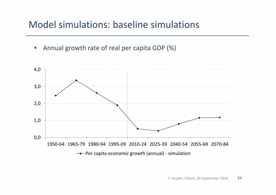
34

• Annual growth rate of real per capita GDP (%)


0,0

1,0

2,0

3,0

4,0

1950-64 1965-79 1980-94 1995-09 2010-24 2025-39 2040-54 2055-69 2070-84

Per capita economic growth (annual) - simulation

F. Heylen, UGent, 26 September 2016

35

• Inequality: Gini coefficient of market income


0,30

0,35

0,40

0,45

0,50

0,55

1965-79 1980-94 1995-09 2010-24 2025-39 2040-54 2055-69 2070-84

Gini - simulation

• Employment rate among older workers

Note: Facts for 2010-2024 concerns the employment rate in 2014.


10

20

30

40

50

60

1950-64 1965-79 1980-94 1995-09 2010-24 2025-39 2040-54 2055-69 2070-84

Employment rate 55-64 - facts Employment rate 55-64 - simulation


Model simulations: counterfactual per capita

output growth scenarios

0,0

1,0

2,0

1980-94 1995-09 2010-24 2025-39 2040-54 2055-69

Baseline simulation No demographic change

0,0

1,0

2,0

1980-94 1995-09 2010-24 2025-39 2040-54 2055-69

Baseline simulation No employment response 55+

No demographic change (since 1950) No response in employment at older age

(since 1980s)

38

Model simulations: counterfactual per capita

output level scenarios (index 1995-2009=100)

100

120

140

160

2000 2010 2020 2030 2040 2050 2060

Per capita output if only technical progress (TFP growth)

Baseline simulation

No demographic change

No employment response 55+

Conclusions

Are OECD countries stuck in a very long period of low

economic growth and rock-bottom real interest rates?

40

If we take policies as constant, and follow the EU AWG projection for technical

change (“risk scenario”) we are inclined to say yes. We then expect:

• Per capita growth rates significantly below the rate of technical change for two to

three more decades.

• Quite flat potential per capita output: growth not higher than 0,5% per year for two to

three more decades.

• Record low interest rate (rate of return to capital) for two or three more decades.

• Rising inequality.



Conclusions

Poor growth in our results is a problem of potential per capita output.

• This conclusion does not exclude that today many countries in Europe also suffer from

weak demand, and deflationary pressure (stagnation from the demand side).

• Additional result (not shown): If a lower bound on the real interest rate exists, and

‘bites’... this could imply even worse per capita output.

Are OECD countries stuck in a very long period of low

economic growth and rock-bottom real interest rates?

Poor growth in our results is a problem of potential per capita output. Main

drivers: the rate of technical change and demographic change.

• Behavioural effects induced by demographic change are not strong enough to counter

arithmetic effects.

• Mobilizing the employment potential can reduce the decline in per capita growth.

• Inequality may rise significantly. Additional simulations reveal no clear/sizable effect

from (rising) inequality on growth though.

Policy implications and recommendations

42

Fiscal policy is key:

• Public investment (infrastructure). Its marginal return is much higher than its cost.

0,0

1,0

2,0

3,0

1980-94 1995-09 2010-24 2025-39 2040-54 2055-69

Baseline simulation Public investment/GDP +1%-point from 2010 onwards


43

• Given the crucial of technical progress (x), promotion of investment in R&D,...

Fiscal policy can contribute � Buyse, Heylen, Schoonackers (2016).

• Subsidies to R&D investment in firms (if well chosen)• Tax incentives • Formation of high-skilled human capital (tertiary education)

• Excessive wage moderation has negative effects on business R&D investment

0,0

1,0

2,0

3,0

1980-94 1995-09 2010-24 2025-39 2040-54 2055-69

Baseline simulation Annual rate of technical change +0,5%-points from 2010 onwards


44

• Given the crucial role of mobilising the employment potential:

• Extended and better targeted taxshift (labour tax cut targeted at older workers and all

low-educated workers is most effective in job creation and in fighting inequality �

Heylen, Van de Kerckhove, Buyse (2015).

• Pension reform with (more) incentives to work longer � Buyse and Heylen (2014),

Buyse, Heylen and Van de Kerckhove (2016)

Given the major impact of demographic change...

• Policies aimed at promotion of fertility

• Migration also includes major opportunities (if immigrants work)

Thank you for the attention.

Further reading: • In Dutch: F. Heylen en P. Van Rymenant, 2016, “Langdurige stagnatie in België? Hoe reëel is de

mogelijkheid, en wat zijn de drijvende krachten?”, www.sherppa.be

• F. Heylen, P. Van Rymenant, B. Boone en T. Buyse, 2016, “On the possibility and driving forces of

secular stagnation: A general equilibrium analysis applied to Belgium”, Working Paper, Faculty of

Economics and Business Administration, Ghent University, N° 2016/919.

45

46

ReferencesBernanke, B. (2015), “Why are interest rates so low, part 2: Secular stagnation”, Ben Bernanke’s Blog, March 31.

Buyse, T. and Heylen, F. (2015), “Een structurele hervorming van het Belgische pensioensysteem. Macro-economische effecten, beleids-aanbevelingen en reflecties op de voorstellen van de Commissie Pensioenhervorming 2020-2040”, Documentatieblad, Federale Overheidsdienst Financiën (België), 74(4), p. 1-18

Buyse, T., Heylen, F. and Van de Kerckhove, R. (2016), “Pension reform in an OLG model with heterogeneous abilities”, Journal of Pension Economics and

Finance, forthcoming.

Buyse, T., Heylen, F. and Schoonackers, R. (2016), “On the role of public policies and wage formation for private investment in R&D: a long-run panel analysis”, Working Paper Research, National Bank of Belgium, N°292.

Eggertsson, G. and Mehrotra, N. (2014), “A model of secular stagnation”, NBER Working Paper, Cambridge MA, n°20574.

Goodhart, C. and Erfurth, P. (2014), “Demography and economics: Look past the past”, VoxEU.org, 4 November.

Fernald, J. and Jones, C. (2014), “The future of US economic growth”, American Economic Review: Papers & Proceedings 2014, 104, 44-49.

Gordon, R., 2014, The turtle’s progress: Secular stagnation meets the headwinds, in Teulings and Baldwin (eds.), Secular Stagnation: Facts, Causes and Cures, CEPR and Vox.Eu, 47-59.

Gordon, R.J. (2015), “Secular stagnation: A supply-side view", American Economic Review: Papers & Proceedings 2015, 105, 54-59.

Heylen, F. and Van de Kerckhove, R. (2013)“Employment by age, education, and economic growth: effects of fiscal policy composition in generalequilibrium”, B.E. Journal of Macroeconomics (Advances), 13(1), p. 49-103

Heylen, F., Van de Kerckhove, R. and Buyse, T. (2015), “Begrotingsbeleid voor werkgelegenheid en groei zonder ongelijkheid’, Economisch Statistische

Berichten, N° 4717, 10 september 2015, p. 528-531

IMF, 2015, Where are we headed? Perspectives on potential output, World Economic Outlook, April, p. 69-110.

Kanbur, R. and Stiglitz, J. (2015), “Wealth and income distribution: New theories needed for a new era”, VoxEU.org, 18 August.

Krueger, D. and A. Ludwig, 2007, ““On the consequences of demographic change for rates of return to capital, and the distribution of wealth and welfare”, Journal of Monetary Economics, 54, 49-87.

Ludwig, A., Schelke, T., Vogel, E. (2012),“Demographic change, human capital and welfare”, Review of Economic Dynamics, 94-107.

Krugman, P. (2014), “Four observations on secular stagnation”, in Teulings, C. and Baldwin, R. (Eds), Secular Stagnation: Facts, Causes and Cures, CEPR Press and VoxEU.org., 61-68.

Mokyr, J. (2014), “Secular stagnation? Not in your life”, in Teulings, C. and Baldwin, R. (Eds), Secular Stagnation: Facts, Causes and Cures, CEPR Press and VoxEU.org., London, 83-89.

OECD (2015), In It Together: Why Less Inequality Benefits All, OECD Publishing, Paris.

Piketty, T. (2014), Capital in the Twenty-First Century”, Harvard University Press.

Solt, F. (2014), "The standardized world income inequality database", Social Science Quarterly, forthcoming, http://myweb.uiowa.edu/fsolt/swiid/swiid.html.

Summers, L., 2014, “Reflections on the ‘New Secular Stagnation Hypothesis’”, in Teulings and Baldwin (eds.), Secular Stagnation: Facts, Causes and Cures, CEPR and Vox.Eu, p. 27-38.

Summers, L. (2015), “Demand side secular stagnation", American Economic Review: Papers & Proceedings, 105, 60-65.

47

500000

1500000

2500000

3500000

1948 1963 1978 1993 2008 2023 2038 2053

Children (age 0-14, left axis) Elderly (65 and older, left axis)

5500000

6000000

6500000

7000000

7500000

8000000

1948 1963 1978 1993 2008 2023 2038 2053Working age population (15-64)

Data : Federal Planning Bureau,

”Bevolkingsvooruitzichten 2016-

2061”

Appendix: demography and projections for future demography in Belgium

Secular stagnation in Belgium? - serv.be · Secular stagnation in Belgium? ... As we saw in the...

Documents

Transcript of Secular stagnation in Belgium? - serv.be · Secular stagnation in Belgium? ... As we saw in the...