Seashells. This presentation presents a method for modeling seashells. Why seashells you ask ? Two...
25
Seashells
-
Upload
lydia-cameron -
Category
Documents
-
view
226 -
download
1
Transcript of Seashells. This presentation presents a method for modeling seashells. Why seashells you ask ? Two...
Seashells
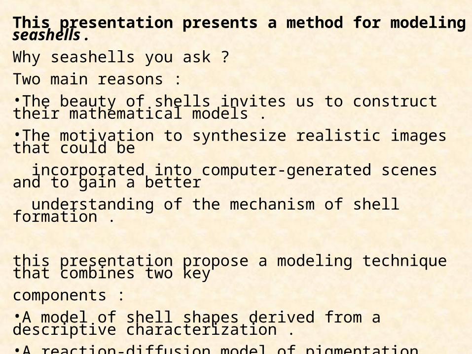
This presentation presents a method for modeling seashells .
Why seashells you ask ?
Two main reasons :•The beauty of shells invites us to construct their mathematical models .•The motivation to synthesize realistic images that could be
incorporated into computer-generated scenes and to gain a better
understanding of the mechanism of shell formation .
this presentation propose a modeling technique that combines two key
components :•A model of shell shapes derived from a descriptive characterization .•A reaction-diffusion model of pigmentation patterns .
The results are evaluated by comparing models with real shells .

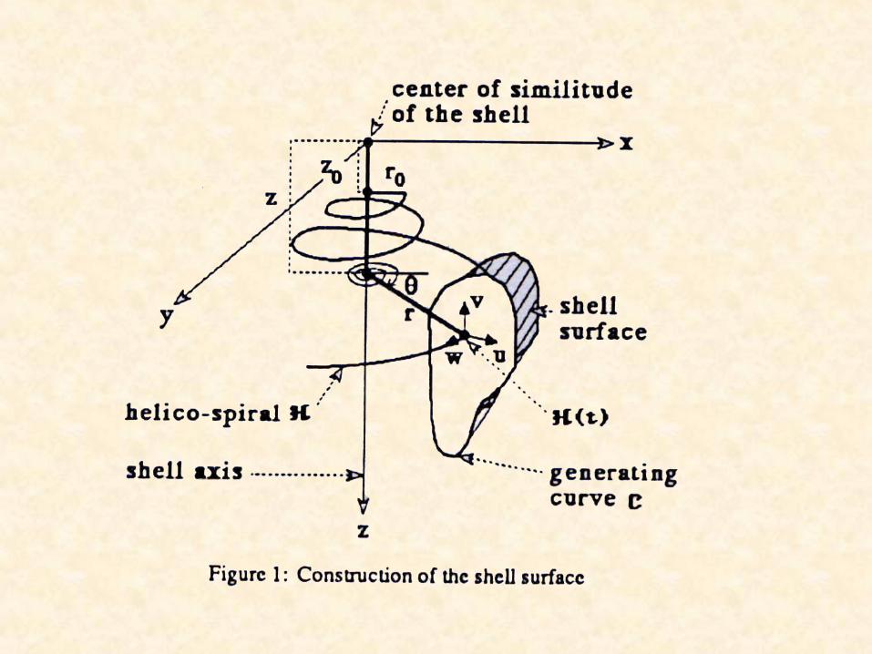
Modeling Shell Geometry (part 1)
The surface of any shell may be generated by the
revolution about a fixed axis of a closed curve , which ,
Remaining always geometrically similar to itself , and
increases its dimensions continually .
A shell is constructed using these steps:• the helico-spiral .• the generating curve .• Incorporation of the generating curve into the model.•Construction of the polygon mesh• modeling the sculpture on shell surfaces .
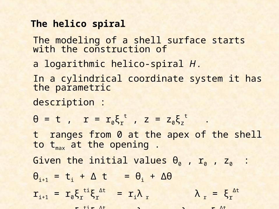
The helico spiral
The modeling of a shell surface starts with the construction of
a logarithmic helico-spiral H .
In a cylindrical coordinate system it has the parametric
description :
θ = t , r = r0ξrt , z = z0ξz
t .
t ranges from 0 at the apex of the shell to tmax at the opening .
Given the initial values θ0 , r0 , z0 :
θi+1 = ti + Δ t = θi + Δθ
ri+1 = r0ξrtiξr
Δt = riλ r λ r = ξrΔt
zi+1 = z0ξztiξz
Δt = ziλ z λ z = ξzΔt
In many shells , parameters λ r , λ z are the same .
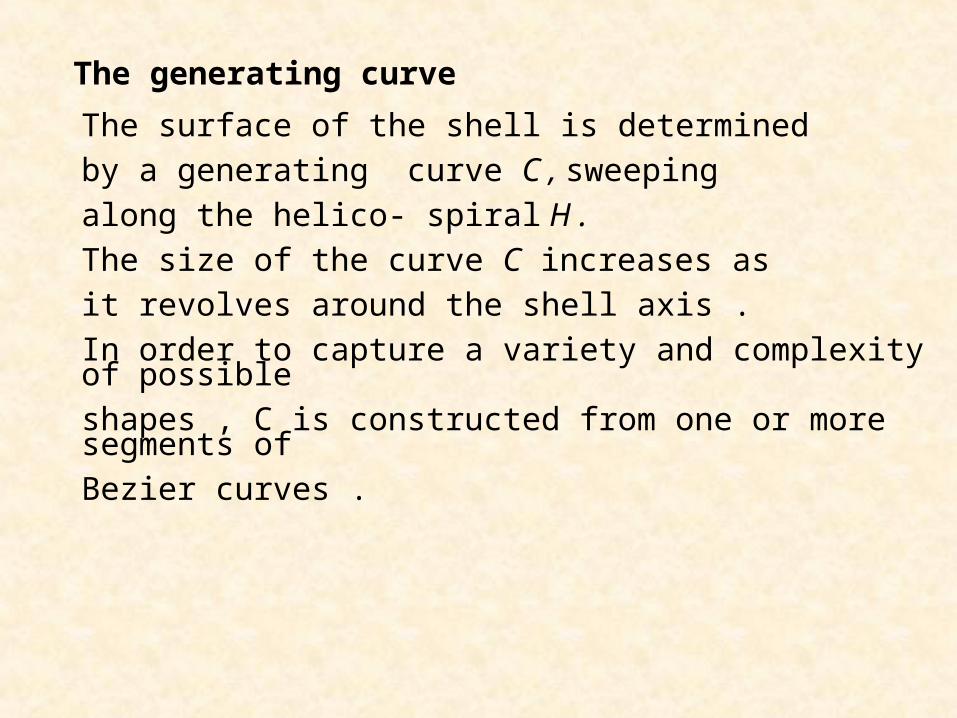
The generating curve
The surface of the shell is determined
by a generating curve C , sweeping
along the helico- spiral H .
The size of the curve C increases as
it revolves around the shell axis .
In order to capture a variety and complexity of possible
shapes , C is constructed from one or more segments of
Bezier curves .
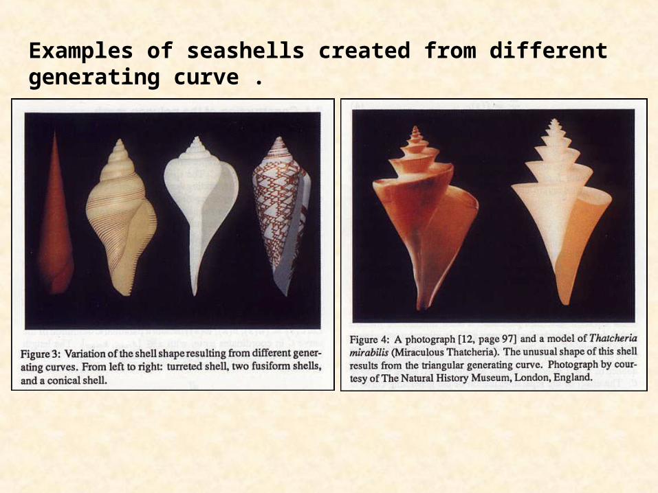
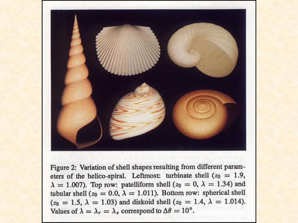
Examples of seashells created from different generating curve .
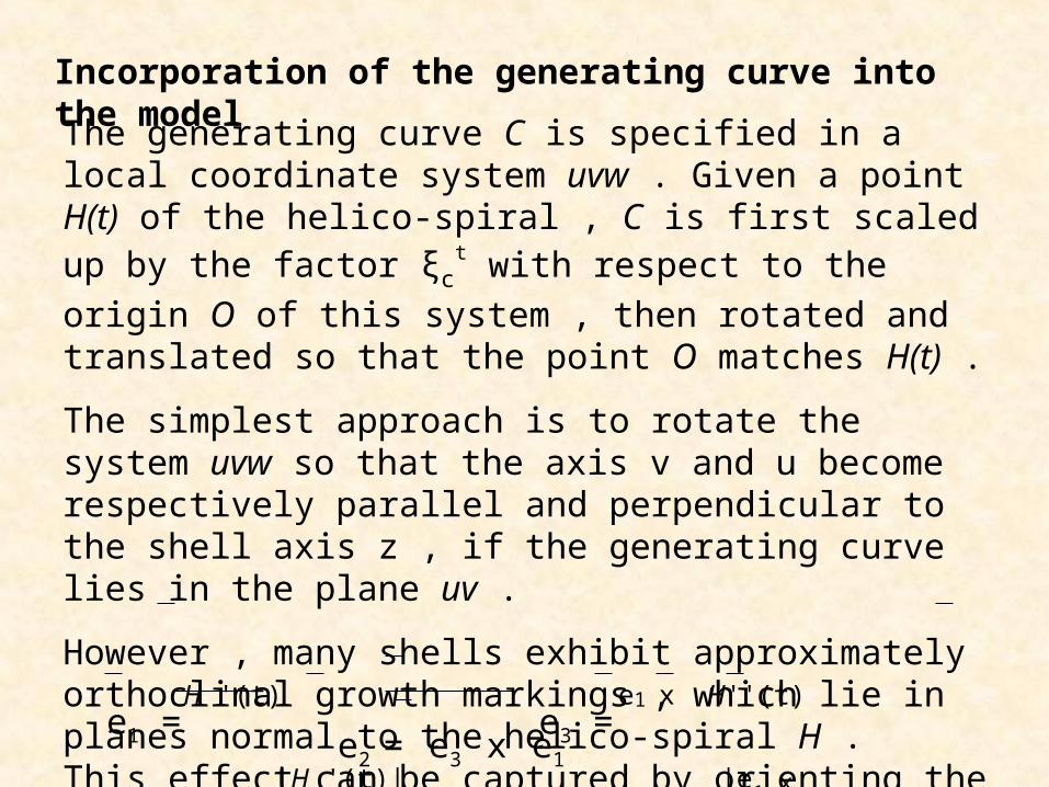
Incorporation of the generating curve into the model
The generating curve C is specified in a local coordinate system uvw . Given a point H(t) of the helico-spiral , C is first scaled up by the factor ξc
t with respect to the origin O of this system , then
rotated and translated so that the point O matches H(t) .
The simplest approach is to rotate the system uvw so that the axis v and u become respectively parallel and perpendicular to the shell axis z , if the generating curve lies in the plane uv .
However , many shells exhibit approximately orthoclinal growth markings , which lie in planes normal to the helico-spiral H . This effect can be captured by orienting the axis w along the vector e1 , aligning the axis u with the principal normal vector e2 .
H '(t)
e1 x H''(t)
e1 = e3 = e2 = e3 x e1
|H '(t)| |e1 x H''(t)|
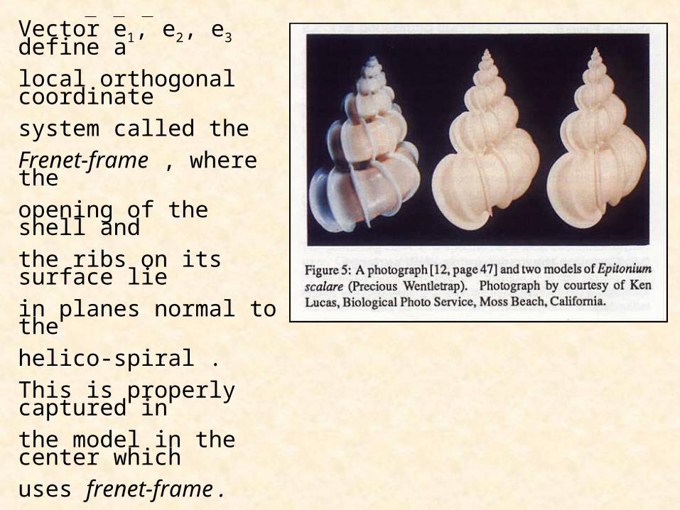
Vector e1, e2, e3 define a
local orthogonal coordinate
system called the
Frenet-frame , where the
opening of the shell and
the ribs on its surface lie
in planes normal to the
helico-spiral .
This is properly captured in
the model in the center which
uses frenet-frame .
The model on the right
incorrectly aligns the
generating curve with the
shell axis .
Construction of the polygon meshIn the mathematical sense , the surface of the shell is completely
defined by the generating curve C, sweeping along the helico-spiral H.
The mesh is constructed by specifying n+1 points on the
generating curve , and connecting corresponding points for
consecutive positions of the generating curve .
The sequence of polygons spanned between a pair of adjacent
generating curves is called a rim .
For pigmentation patterns equations (which will be explained later on) , it is best if the space in which they operate is discretized uniformly .This corresponds to the partition of the rim into polygons evenly spaced along the generating curve .
Let C(s) = ( u(s) , v(s) , w(s) ) a parametric definition of the curve
C in cordinates uvw , with s [smin , smax ] .
dl = f (s) , ds
du 2 dv 2 dw 2
f(s) = + + ds ds ds
smin
L = ∫ f (s) ds smax
ds 1 = dl f (s)
A method for achieving discretized uniformly space .
The length of an arc of C is related to an increment of
parameter s by the equations :
The total length L of C can be found by integrating f (s) in the interval [smin , smax ] :
1(
2(
3(
4(
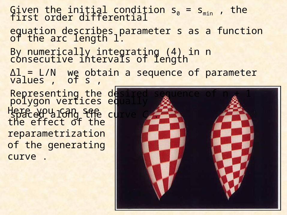
Given the initial condition s0 = smin , the first order differential
equation describes parameter s as a function of the arc length l.
By numerically integrating (4) in n consecutive intervals of length
Δl = L/N we obtain a sequence of parameter values , of s ,
Representing the desired sequence of n + 1 polygon vertices equally
spaced along the curve C .
Here you can see the effect of the reparametrization of the generating curve .
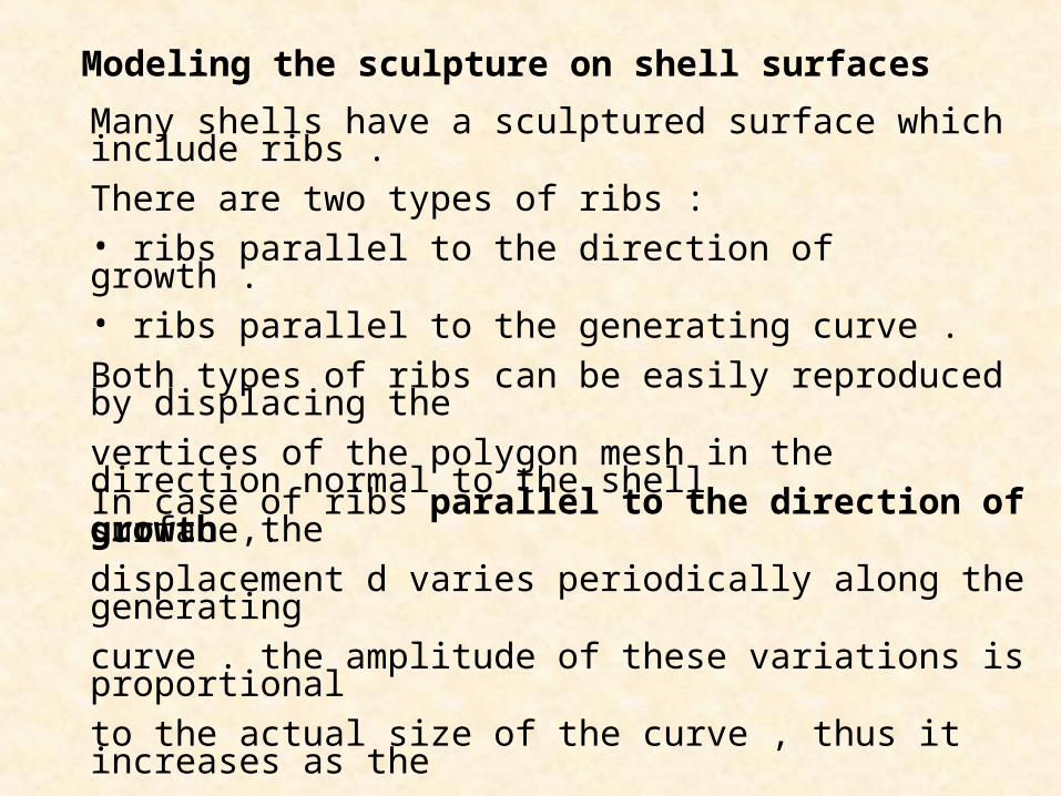
Modeling the sculpture on shell surfaces
Many shells have a sculptured surface which include ribs .
There are two types of ribs :• ribs parallel to the direction of growth . • ribs parallel to the generating curve .
Both types of ribs can be easily reproduced by displacing the
vertices of the polygon mesh in the direction normal to the shell
surface .
In case of ribs parallel to the direction of growth ,the
displacement d varies periodically along the generating
curve . the amplitude of these variations is proportional
to the actual size of the curve , thus it increases as the
shell grows .
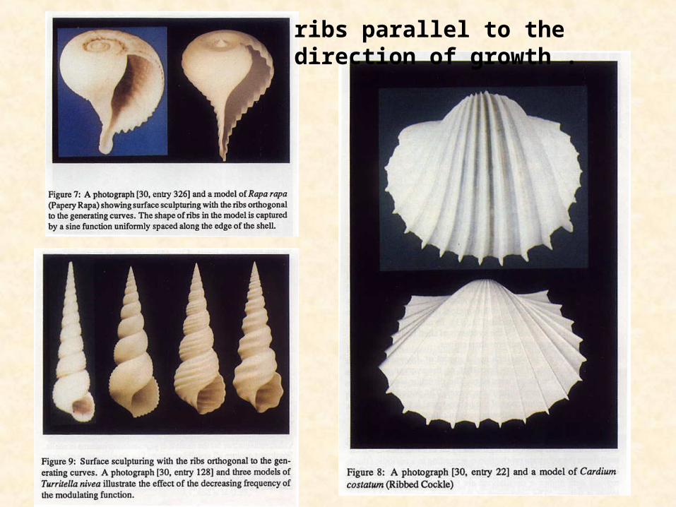
ribs parallel to the direction of growth .
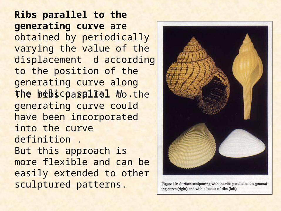
Ribs parallel to the generating curve are obtained by periodically varying the value of the displacement d according to the position of the generating curve along the helico-spiral H .
The ribs parallel to the generating curve could have been incorporated into the curve definition . But this approach is more flexible and can be easily extended to other sculptured patterns.
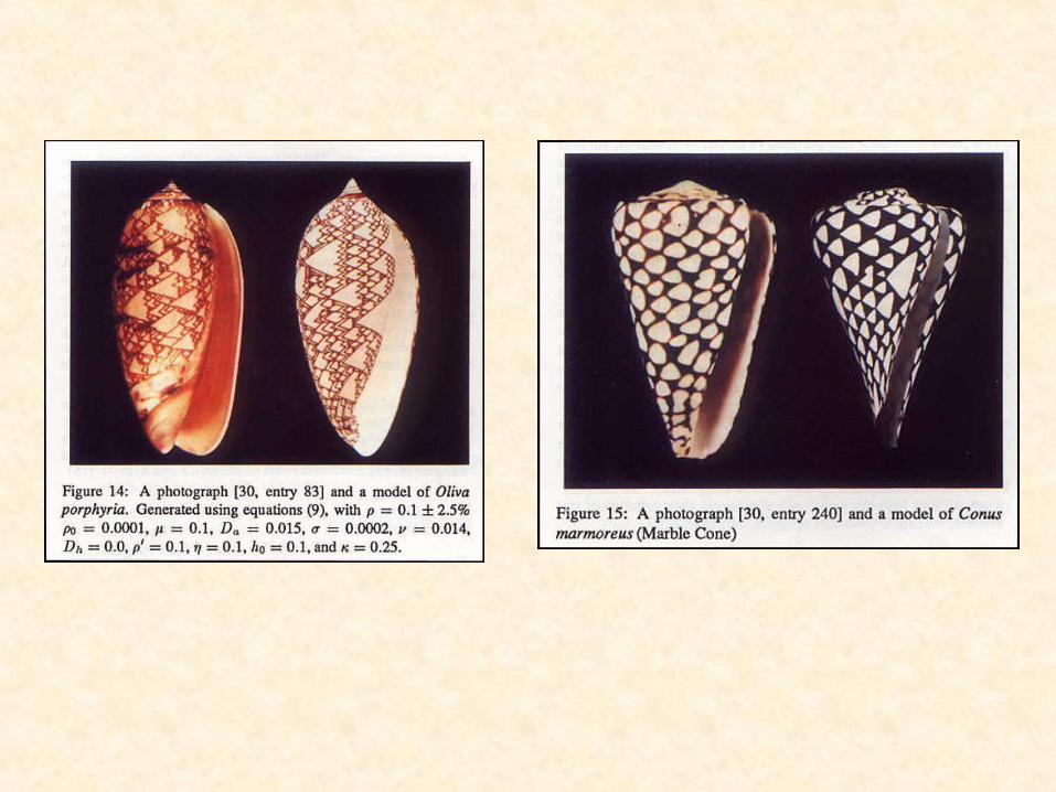
Generation of pigmentation patterns (part2)
Pigmentation patterns constitute an important aspect of shell
appearance because they show enormous diversity , which
may differ in details even between shells of the same species .
In this presentation pigmentation patterns are captured using
a class of reaction-diffusion models .
Generally , we group our models into two basic categories :
• Activator–substrate model .
• Activator–inhibitor model .
= ρs( + ρ0 ) – μa + Da ∂ t 1 + ka2 ∂ x2
= σ - ρs( + ρ0 ) – νs + Da ∂ t 1 + ka2 ∂ x2
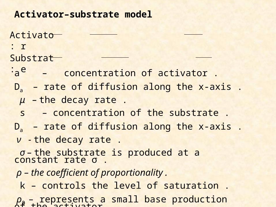
Activator–substrate model
a – concentration of activator .
Da – rate of diffusion along the x-axis .
μ – the decay rate .
s – concentration of the substrate .
Da – rate of diffusion along the x-axis .
ν - the decay rate .
σ – the substrate is produced at a constant rate σ .
ρ – the coefficient of proportionality .
k – controls the level of saturation .
ρ0 – represents a small base production of the activator ,
needed to initiate the reaction process .
Activator:
Substrate:
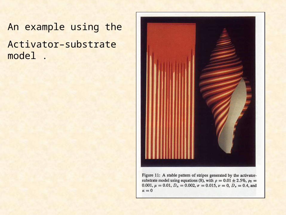
An example using the
Activator–substrate model .
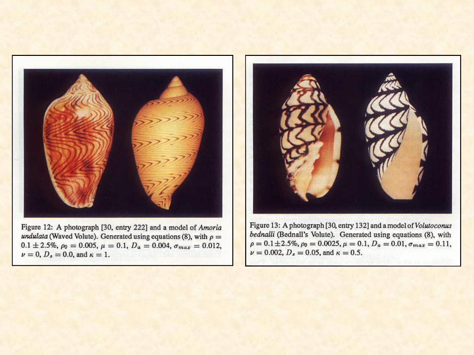
Activator–inhibitor model .
As you can see in the picture colliding waves is essential.
Observation of the shell indicates that the number of
traveling waves is approximately constant over time , this
suggests a global control mechanism that monitors the total
amount of activators in the system and initiartes new waves
when its concentration becomes too low .
∂ a ρ a2 ∂ 2a = ( + ρ0 ) – μa + Da ∂ t h+h0 1 + ka2 ∂ x2
= σ + ρ - h + Dh ∂ t 1 + ka2 c ∂ x2
= ∫ adx - ŋc dt xmax - xmin xmin
Conclusion
This presentation presents a comprehensive model of seashells ,
There are still some problems for further research :
• proper modeling of the sea shell opening .
• modeling of spikes
• capturing the the thickness of shell walls .
• alternative to the integrated model
• improved rendering
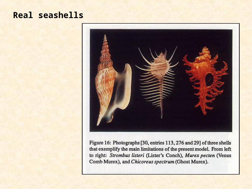
Real seashells
The end

![Practice sounds [S], [s] She sells seashells by the seashore. The shells she sells are surely seashells, so if she sells shells on the sea shore, Im sure.](https://static.fdocuments.net/doc/165x107/5517f595550346c6568b4d65/practice-sounds-s-s-she-sells-seashells-by-the-seashore-the-shells-she-sells-are-surely-seashells-so-if-she-sells-shells-on-the-sea-shore-im-sure.jpg)