RURALS: Review of Undergraduate Research in Agricultural and RURALS: Review of Undergraduate Research in Agricultural and

Life Sciences Life Sciences

Volume 1 Issue 1 Article 1

August 2006

Estimation of Heat Transfer Coefficients of Cooked Boneless Estimation of Heat Transfer Coefficients of Cooked Boneless

Ham Ham

Kimberly Ryland University of Nebraska-Lincoln, Kimberly.ryland@gmail.com

Lijun Wang University of Nebraska-Lincoln, lwang5@unl.edu

Alejandro Amézquita University of Nebraska-Lincoln, aamezquita2@unl.edu

Curtis L. Weller University of Nebraka-Lincoln, cweller1@unl.edu

Follow this and additional works at: https://digitalcommons.unl.edu/rurals

Recommended Citation Recommended Citation Ryland, Kimberly; Wang, Lijun; Amézquita, Alejandro; and Weller, Curtis L. (2006) "Estimation of Heat Transfer Coefficients of Cooked Boneless Ham," RURALS: Review of Undergraduate Research in Agricultural and Life Sciences: Vol. 1 : Iss. 1 , Article 1. Available at: https://digitalcommons.unl.edu/rurals/vol1/iss1/1

This Article is brought to you for free and open access by the Agricultural Economics Department at DigitalCommons@University of Nebraska - Lincoln. It has been accepted for inclusion in RURALS: Review of Undergraduate Research in Agricultural and Life Sciences by an authorized administrator of DigitalCommons@University of Nebraska - Lincoln.

Estimation of Heat Transfer Coefficients of Cooked Boneless Ham Estimation of Heat Transfer Coefficients of Cooked Boneless Ham

Cover Page Footnote Cover Page Footnote Funding for this project was provided through the University of Nebraska-Lincoln Agricultural Research Division, Undergraduate Honors Student Research Program. The authors express their gratitude to all who contributed to the project especially for their patience and teaching! Author biographies are listed at the end of the article. Review coordinated by Professor Lloyd B. Bullerman, Department of Food Science and Technology, University of Nebraska-Lincoln.

This article is available in RURALS: Review of Undergraduate Research in Agricultural and Life Sciences: https://digitalcommons.unl.edu/rurals/vol1/iss1/1

1. Introduction An estimated 76 million illnesses, 325,000 hospitalizations, and 5,000 deaths are caused by food-borne diseases each year in the United States (Mead et al., 1999). Considering the severity of potential public health problems associated with poor food safety practices, the Food Safety and Inspection Service (FSIS) of the U.S. Department of Agriculture (USDA) requires federally inspected meat processors to implement HACCP (Hazard Analysis and Critical Control Points) plans for all of their products.

In this context, cooling immediately after cooking of large ready-to-eat (RTE) meat products is an important processing step, and must be considered in development and implementation of HACCP plans. Rapid cooling of large RTE meat products is critical to prevent the potential outgrowth of spore-forming food-borne pathogens that survive the heat treatment. In 1999, the FSIS established time-temperature compliance guidelines for the cooling of RTE meat and poultry products (USDA, 1999). The FSIS proposed that by following these guidelines, allowable growth of Clostridium perfringens would be limited to a 1-log10 multiplication. In the case of cured products (i.e. at least 100 ppm ingoing sodium nitrite), the guidelines recommend that the product internal temperature be reduced from 54.4°C to 26.6°C in less than 5 h, and from 26.6°C to 7.2°C in the next 10 h (15 h total cooling time). For non-cured products, the guidelines recommend that the product internal temperature be reduced from 54.4°C to 26.6°C in less than 1.5 h, and from 26.6°C to 4.4°C in the next 5 h (6.5 h total cooling time).

In general, air chilling is the most common method for cooling of RTE meats in small meat-processing facilities. Typically, once the products are removed from the smokehouse at the conclusion of the cooking cycle, they are showered with tap water for 20 to 30 min, and finally placed in a chilling room. Inside the chilling room, cold air is forced through and over the products. This process involves convective heat exchange between the product surface and the cold airflow, and heat conduction through the product body. Product size and proximate chemical composition (i.e. mainly protein, fat and moisture percentages) determine the heat conduction rate through the body. Meanwhile product shape and arrangement, air velocity, air temperature and relative humidity inside the chilling room control the heat exchange rate between product surface and cooling medium (cold air).

In-depth understanding of heat transfer phenomena between product surface and cooling medium (convective heat transfer) is fundamental for accurate predictions of cooling times and rates. This information is very important as a quantitative tool for general food safety applications. In this study, two

1

Ryland et al.: Estimation of Heat Transfer Coefficients of Ham

Published by DigitalCommons@University of Nebraska - Lincoln, 2006

experimental methods were used to determine the convective heat transfer coefficient (hc) of a 2.25 kg (5 lb) processed boneless cooked ham in forced convection cooling conditions. To accomplish this, a block of aluminum shaped like a commercial ham was used as a theoretical standard from which hc could be estimated. Measured hc values were compared against well-established empirical correlations for ellipsoidal and other anomalous geometries.

1.1 Objective The objective of this study was to determine the convective heat transfer coefficient hc for an aluminum block of known standard ham shape during cooling, and to compare the experimental results with tabulated values and theoretically calculated values using well-known existing correlations. 2. Materials and Methods 2.1 Nomenclature For purposes of brevity and clarity the following nomenclature and corresponding metric units are used throughout. a minor semi-axes of the ellipsoidal body in Figure 3 (m) A area (m2)

major semi-axis of the ellipsoidal body in Figure 3 (m) Biot number

bBi ( )cBi h D k=

characteristic dimension (m) heat transfer coefficient (W/m

Dh 2°C)

mass (kg) Nusselt number

mNu ( )cNu h D k=

Pr Prandtl number ( )Pr c kμ=

Rayleigh number ( )

Reynolds number

Ra Ra Gr Pr= ⋅

Re ( )Re uDρ μ=

relative humidity time (s) temperature (°C) air velocity (m/s) volume (m

RHtTuV 3) λ latent heat (J/kg) μ viscosity (Pa s) ρ density (kg/m3)

2

RURALS: Review of Undergraduate Research in Agricultural and Life Sciences, Vol. 1 [2006], Iss. 1, Art. 1

https://digitalcommons.unl.edu/rurals/vol1/iss1/1

2.1.1 Subscripts 0 initial value

ambient or air aluminum

convection characteristic dimension

aalumcDfc forced convection

natural convection surface evaporation water

ncsvw 2.2 Aluminum ham model system A 'ham-shaped’ block of aluminum was used as a theoretical model. The model was milled from a solid block of grade-6061 aluminum at the Department of Biological Systems Engineering's machine shop (University of Nebraska-Lincoln, Lincoln, NE, USA). Its shape was modeled after a 2.25 kg commercial boneless ham. Dimensions of the aluminum ham model were: 23.5 cm long × 8.9 cm thick

12.7 cm wide, with rounded ends (radii 6.4 cm) and filleted edges (radii 2.5 cm). A small hole (0.325 cm diameter) through the center of its length allowed for the placement of a rigid multisensor temperature-profiling probe which will be described later. Drawings were constructed using SolidWorks

×

® 2001 software (SolidWorks Corporation, Concord, MA, USA) from which a surface area of 0.1215 m2 was calculated. Figure 1 shows an schematic of the aluminum model.

Figure 1. Drawing of Aluminum Ham Model (created in SolidWorks® 2001). Dimensions: 23.5 cm long 8.9 cm thick × 12.7 cm wide. ×

3

Ryland et al.: Estimation of Heat Transfer Coefficients of Ham

Published by DigitalCommons@University of Nebraska - Lincoln, 2006

2.3 Data acquisition system A 32-channel data acquisition (DAQ) system controlled by LabVIEW 6.1 software (National Instruments Corporation, Austin, TX, USA) was used for collection of experimental data necessary for validation experiments. The DAQ system consisted of a SCXI-1000 chassis that held a SCXI-1102 32-channel thermocouple amplifier module connected to a SCXI-1303 terminal block. The output signals were transmitted to a laptop computer through a DAQCard-AI-16XE-50 card. A program written in LabVIEW 6.1 controlled the DAQ system and recorded the data in real time. The program had a user-friendly interface where the experimenter simply specified the name of the output data storage file and the time interval over which experimental data was to be recorded.

A total of 11 sensors were connected to the 32-channel amplifier module for data collection, including: • One FMA-904-V air velocity transducer (Omega Engineering, Inc., Stamford,

CT, USA), • One HX303V RH/Temperature transmitter (Omega Engineering, Inc.), • One top-loading balance (TR-series) for collection of dynamic weight loss

data (Denver Instrument Company, Arvada, CO, USA), • One rigid multisensor probe consisting of 6 thermocouples inside a 0.318 cm

diameter 316 stainless steel sheath (Omega Engineering, Inc.) used for determining the temperature profile of the aluminum ham model (see Multisensor Temperature Profiling Probe), and

• One TMQSS-062G-6 single thermocouple (Omega Engineering, Inc.) used for verification of air temperature measurement.

2.4 Multisensor temperature profiling probe In order to determine the hc value, it was necessary to continuously record the temperature profile of the ‘ham’ model and the temperature of the environment. To verify the calculations, temperature data from multiple locations within the ‘ham’ was required. To capture this data, a custom-built Omega® profile probe was used.

The custom-ordered Omega® profile probe consisted of 6 individually stranded type-T thermocouples placed inside a single 0.318 cm outer sheath made of 316 stainless steel. This design allowed for temperature profiling at various points along a single axis through the center of the ‘ham’. The probe was 45.72 cm long with thermocouples placed at 0, 12.70, 15.24, 17.78, 20.32, and 22.86 cm from the tip (thermocouples numbered T1 to T6—see Figure 2). When placed in the ‘ham’, thermocouple number 6 (22.86 cm from the base) was positioned

4

RURALS: Review of Undergraduate Research in Agricultural and Life Sciences, Vol. 1 [2006], Iss. 1, Art. 1

https://digitalcommons.unl.edu/rurals/vol1/iss1/1

directly at the ‘ham’ model's center with thermocouples 2 through 5 located at 2.54 cm intervals within the ham. Thermocouple number 1 was located in the open air recording the chamber temperature (see Figure 2). The probe was rated at 200oC maximum temperature.

Figure 2. Placement of Custom-built multisensor temperature profiling probe (Omega Engineering, Inc.); thermocouples T1-T6 inside of aluminum ham model.

2.5 Methods for estimation of convective heat transfer coefficient Experimental measurement of hc was based on two different methods: (1) a quasi-steady state method based on the lumped parameter condition concept (Arce and Sweat, 1980; Rahman, 1995), and (2) a method described by Kondjoyan and Daudin (1997) based on constant drying rates of fully wetted bodies. 2.5.1 Method 1: The first method is valid when heat conduction can be ignored (Biot number < 0.1). Thus a material of high thermal conductivity was required (i.e. aluminum). For this method, the aluminum model was heated up to 80°C in an IsotempTM oven (Fischer Scientific, Hampton, NH, USA) to a center temperature of 71.1 1.7°C. The heated model was then immediately placed in an Aminco-Aire environmental chamber (Parameter Generation & Control, Inc., Black Mountain, NC, USA) where a continuous flow of cold air (T

±

a = 6.47 0.34°C) was forced around the aluminum model. Control of airflow inside the environmental chamber was achieved by placing an additional fan on the bottom of the chamber directed upward towards the ham model. Additionally, an artificial wind tunnel (1.3 m long) of square cross-sectional area (0.55 m × 0.55 m) was created using rigid cardboard deflectors.

±

Temperature data were recorded every 30 s using the previously described DAQ system during the entire cooling process. Values of hc were obtained by non-linear regression (SAS PROC NLIN) in the Statistical Analysis System

5

Ryland et al.: Estimation of Heat Transfer Coefficients of Ham

Published by DigitalCommons@University of Nebraska - Lincoln, 2006

Release 8.2 (SAS Institute, Inc., Cary, NC, USA), using the Marquardt updating formula. The non-linear model used was that corresponding to the lumped parameter condition (Equation 1). Four replicates of the experiment were carried out.

( )0 exp c sa a

alum alum

h AT T T T tm c

⎛ ⎞= + − −⎜

⎝ ⎠⎟ (1)

2.5.2 Method 2: The second method was based upon the drying of a fully-wetted body in an air current with constant properties. This method accounted for simultaneous heat and mass transfer during cooling. The heat transfer coefficient was determined during the constant drying-rate period, using the equations described by Kondjoyan and Daudin (1997). For that purpose, the aluminum ham model was wrapped in strips of newspaper and then coated with a 5-mm thick layer of Plaster of Paris and soaked in water overnight. Subsequently, the wetted model was suspended on a top-loading balance inside the wind tunnel previously described with a continuous flow of air directed around the plaster-covered model. During the entirety of testing the aluminum ham model was kept in thermal equilibrium with the chamber, which in turn was kept at constant dry bulb and wet bulb temperatures. The top-loading balance was connected to the DAQ system and dynamic weight loss was recorded every 30 s during the entire drying process. Air velocity, relative humidity and air temperature were also recorded every 30 s. Three replicates of the experiment were carried out. A new SolidWorks® drawing was constructed to calculate the new surface area resulting in 0.1374 m2.

The slope of the plot of weight loss vs. time during the constant-rate period was used for calculations (i.e. slope = wdm dt ). During the constant-rate drying period simultaneous heat and mass transfer can be described mathematically as:

( )c s a sw

v

h A T Tdmdt λ

−= (2)

In Equation 2, the effect of heat transfer by radiation was neglected due to

the low temperatures considered in the study.

6

RURALS: Review of Undergraduate Research in Agricultural and Life Sciences, Vol. 1 [2006], Iss. 1, Art. 1

https://digitalcommons.unl.edu/rurals/vol1/iss1/1

2.6 Empirical correlations for determination of hc as reported in the literature Values of hc measured experimentally by the above-described methodologies were compared with well-known existing correlations for ellipsoidal bodies and other anomalous geometries of similar shape. Relative errors between experimental values and those predicted by the empirical correlations were used as a measure of accuracy of the laboratory methods. 2.6.1 Correlations of Yovanovich: For ellipsoidal shapes, Yovanovich (1987) proposed the following correlation for natural convection (the characteristic dimension in Yovanovich's correlation is the square root of the surface area, sA ):

( ) 1 43.470 0.510s sA Anc

Nu Ra= + , 80 10sARa< < (3)

In the case of forced convection, Yovanovich (1988) proposed the

following correlation: ( ) ( )1 4 1 2 0.566 1 32 0.150 0.350

s sA AfcNu Re Re Prπ π= + +

sA , (4)

2 510 10sARe− < < & 0.71Pr =

Air properties were evaluated at film temperature ( )( )2f s aT T T= − from

tabulated values (Kays and Crawford, 1993). The combined natural and forced convective heat transfer coefficient were

calculated using an empirical correlation proposed by Churchill (1977). This correlation has been used in other studies dealing with cooling of meat products (Davey and Pham, 1997; Wang and Sun, 2002a, b):

( )1 33 3

c nc fch h h= + (5) 2.6.2 Correlations of Smith and coworkers: Smith et al. (Smith et al., 1967; Smith et al., 1971) developed a method for calculating heat transfer coefficients of boneless pressed hams based on their geometries. These researchers derived a relationship based on a pressed ham being modeled as two ellipsoids (see Figure 3).

7

Ryland et al.: Estimation of Heat Transfer Coefficients of Ham

Published by DigitalCommons@University of Nebraska - Lincoln, 2006

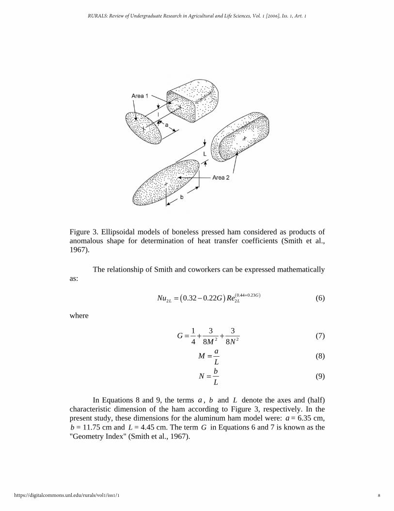
Figure 3. Ellipsoidal models of boneless pressed ham considered as products of anomalous shape for determination of heat transfer coefficients (Smith et al., 1967).

The relationship of Smith and coworkers can be expressed mathematically

as: (6) ( ) (0.44 0.23

2 0.32 0.22 GLNu G Re += − )

2L where

2

1 3 34 8 8

G 2M N= + + (7)

aML

= (8)

bNL

= (9)

In Equations 8 and 9, the terms , and a b L denote the axes and (half)

characteristic dimension of the ham according to Figure 3, respectively. In the present study, these dimensions for the aluminum ham model were: a = 6.35 cm,

= 11.75 cm and b L = 4.45 cm. The term in Equations 6 and 7 is known as the "Geometry Index" (Smith et al., 1967).

G

8

RURALS: Review of Undergraduate Research in Agricultural and Life Sciences, Vol. 1 [2006], Iss. 1, Art. 1

https://digitalcommons.unl.edu/rurals/vol1/iss1/1

3. Results and Discussion 3.1 Results for method 1: Table 1. Environmental conditions of aluminum ham testing (Method 1), forced-air cooling.

Replication

Air Velocity

(m/s) Standard Deviation

Relative Humidity (%)

Standard Deviation

Air (1) Temperature (oC)

Standard Deviation

1 1.00 0.20 81.69 0.81 6.44 0.17 2 1.27 0.20 83.39 0.32 6.53 0.50 3 1.08 0.19 82.97 0.31 6.36 0.29 4 1.36 0.24 83.40 0.35 6.55 0.40

Mean 1.17 0.21 82.86 0.45 6.47 0.34

(1) Dry bulb temperature

Table 1 presents the experimental values of the environmental conditions

inside the Aminco-Aire testing chamber for the 4 replications carried out for Method 1. In general, air velocity was slightly above 1 m/s in all cases, and relative humidity, as well as air temperature, remained fairly constant.

Figure 4 illustrates a typical time-temperature profile obtained for Method

1. As can be observed in this figure, all of the temperatures recorded within the aluminum ham body along its axis resulted in similar values for all times (T3 to T6 in Figure 4). However, as can be observed in Figure 4, temperature values recorded by the thermocouple T2 were slightly below those captured by the remaining sensors. The sensor T2 was located inside the aluminum ham model, at a location close to the surface (see Figure 2). The observation of lower values recorded by T2 indicated that there was a temperature distribution within the aluminum ham body, and therefore, the lumped parameter assumption was violated.

9

Ryland et al.: Estimation of Heat Transfer Coefficients of Ham

Published by DigitalCommons@University of Nebraska - Lincoln, 2006

0

10

20

30

40

50

60

70

80

0 8000 16000 24000 32000 40000 48000 56000

Time (sec)

Tem

pera

ture

(°C

)

T2

T3

T4

T5

T6

Mean 'ham' Temp

Air Temp

Figure 4. Sample temperature profile of aluminum ham testing (replication 1) during forced-air cooling (initial core temperature 71.2°C, air velocity 1.00 m/s, relative humidity 81.69%, air temperature 6.44°C). Table 2. Convective heat transfer coefficient estimated by non-linear regression using a lumped parameter condition approach (Method 1), forced-air cooling.

ReplicationCalculated hc (W/m2 °C)

Standard Deviation

1 5.24 0.0037 2 5.05 0.0025 3 5.09 0.0027 4 5.00 0.0022

Mean 5.10 0.0028 The mean time-temperature curve shown in Figure 4 was used for

estimation of hc values by non-linear regression. Results of non-linear regression (SAS PROC NLIN) from Equation 1 are presented in Table 2. Values of 0.1215 m2, 5.93 kg and 840 J/kg °C for sA , and , respectively, were set as constants during the non-linear regression procedure.

alumm alumc

10

RURALS: Review of Undergraduate Research in Agricultural and Life Sciences, Vol. 1 [2006], Iss. 1, Art. 1

https://digitalcommons.unl.edu/rurals/vol1/iss1/1

3.2 Results for method 2: Table 3. Environmental conditions of plaster-covered aluminum ham testing (Method 2).

Replication

Air Velocity

(m/s) Standard Deviation

Relative Humidity (%)

Standard Deviation

Air (1) Temperature (oC)

Standard Deviation

1 1.13 0.16 82.51 0.38 6.11 0.08 2 1.11 0.20 82.06 0.27 6.12 0.04 3 1.18 0.15 82.51 0.18 6.11 0.05

Mean 1.14 0.17 82.36 0.28 6.11 0.06

(1) Dry bulb temperature Table 3 presents the experimental values of the environmental conditions

inside the Aminco-Aire testing chamber for the 3 replications carried out for Method 2. In general, environmental conditions were very similar to those observed in experiments for Method 1.

Figure 5 illustrates a typical weight loss history obtained for Method 2. As

can be observed in this figure, during the entire cooling process mass loss rate appeared to be relatively constant. This is in compliance with the assumption of a constant drying-rate period upon which Method 2 was based. It was assumed that mass loss was only due to loss of moisture. Therefore, the slope of mass relative to time was used to find hc from Equation 2, using 0.1374 m2 as the value of sA . The observation of constant-rate drying indicated that mass transfer from the plaster-covered model surface to the circulating air was in equilibrium with moisture diffusion from within the plaster layer. Thus, in Equation 2, the value of

sT (°C) was taken as the wet bulb temperature of the air, which was obtained directly from a psychrometric chart using mean values of dry bulb temperature and relative humidity (see Table 3). Similarly, the latent heat of evaporation ( ) was obtained from steam tables at the surface temperature value (

vλ

sT ). A summary of results is presented in Table 4.

11

Ryland et al.: Estimation of Heat Transfer Coefficients of Ham

Published by DigitalCommons@University of Nebraska - Lincoln, 2006

6600

6610

6620

6630

6640

6650

6660

6670

6680

6690

6700

0 8000 16000 24000 32000 40000 48000 56000 64000

Time (sec)

Mas

s (g

)

Figure 5. Sample weight loss history of fully wetted plaster-covered aluminum ham testing (replication 2) during air drying (initial core temperature 6.24°C, air velocity 1.11 m/s, relative humidity 82.06%, initial mass 6,690.9 g).

Table 4. Calculated results from fully wetted plaster-covered aluminum ham testing (Method 2).

Replicate wdm dt

(g/s) Standard Deviation

aT (°C)

Standard Deviation

sT (°C)

vλ (J/g)

hc (1)

(W/m2°C) Standard Deviation

1 0.00068 0.0007 6.11 0.08 4.9 2489.81 10.18 2 0.00064 0.0002 6.12 0.04 4.9 2489.81 9.51 3 0.00064 0.0001 6.11 0.05 4.9 2489.81 9.58

Mean 0.00065 0.0003 6.11 0.06 4.9 2489.81 9.73 0.37 (1) Calculated from Equation 2

12

RURALS: Review of Undergraduate Research in Agricultural and Life Sciences, Vol. 1 [2006], Iss. 1, Art. 1

https://digitalcommons.unl.edu/rurals/vol1/iss1/1

3.3 Comparison with Empirical Correlations: Table 5. Estimated hc values using well-established empirical correlations for ellipsoidal bodies and other anomalous geometries of similar shape.

Aluminum model Plaster-covered model Correlation DNu (1)

ch (W/m2°C)

DNu (1)ch

(W/m2°C) Yovanovich (natural convection) (2)

45.08

3.17

30.69

2.03

Yovanovich (forced convection) (3)

140.33 9.86 143.03. 9.45

Combined (Yovanovich natural and forced) (4)

9.97 9.49

Smith et al. (5)

29.41 8.09 31.52 7.80

(1) The characteristic dimension ( D ) varies according to each correlation. In Yovanovich's correlations sD A= , whereas in Smith's correlation 2D L= (2) Equation 3 (3) Equation 4 (4) Equation 5 (5) Equation 6

Table 5 presents a summary of hc values calculated from the empirical

correlations used for comparison with experimental data in this study. Table 6 presents a summary of relative errors between mean values of experimentally determined hc (see Tables 2 and 4), and those estimated from empirical correlations presented in Table 5.

13

Ryland et al.: Estimation of Heat Transfer Coefficients of Ham

Published by DigitalCommons@University of Nebraska - Lincoln, 2006

Table 6. Relative errors between values of convective heat transfer coefficients determined experimentally by two methods and those estimated from well-established empirical correlations. Compared Values

Relative Error (%) Method 1 (1)

Relative Error (%) Method 2 (2)

Experimental vs. Yovanovich (combined)

48.84 (3)

2.52 (4)

Experimental vs. Smith

36.96 (5) 24.74 (6)

(1) Quasi-steady state method (2) Constant drying-rate method (3) Yovanovich's combined aluminum compared with experimental value of Method 1 (4) Yovanovich's combined plaster-covered compared with experimental value of Method 2 (5) Smith's aluminum compared with experimental value of Method 1 (6) Smith's plaster-covered compared with experimental value of Method 2

As can be observed from Table 6, the quasi-steady state method (Method

1) grossly underestimated hc values when compared with empirical correlations, resulting in very high relative errors. This may have occurred because the aluminum model was too large, violating the lumped-parameter assumption of a uniform temperature distribution throughout the body. This was previously discussed in Figure 4, in which the temperature sensor T2 (placed inside the ham model close to the surface) captured lower temperature values than the other sensors along the model axis. These temperature differences were as high as 11.9°C (in replication 1), particularly during the first stages of the cooling process. The quasi-steady approach has been successfully used in other meat processing applications involving smaller products such as hamburgers (Millsap and Marks, 2002). However, for products as large as a 2.25-kg ham, this methodology appeared inadequate in the present study.

Other possible sources of error could have been heat conduction through the ham caused by the large stainless steel probe. Although probe testing showed that the air chamber temperature readings (T1) were not significantly affected by heat conduction through the probe (data not shown), it is possible that heat conduction played a more significant role at other thermocouple locations, especially at T2 since it was located so close to the surface.

Conversely, hc values obtained from the experimental methodology proposed by Kondjoyan and Daudin (1997), which involves simultaneous heat

14

RURALS: Review of Undergraduate Research in Agricultural and Life Sciences, Vol. 1 [2006], Iss. 1, Art. 1

https://digitalcommons.unl.edu/rurals/vol1/iss1/1

and mass transfer, resulted in closer agreement with empirical correlations. Deviations between experimental and estimated (from correlations) data may have occurred because of the differences in shape assumptions made by the two empirical correlations.

The relative error obtained when comparing experimental values obtained with Method 2 and the empirical correlations proposed by Yovanovich (1987; 1988) was only 2.52%. This result indicates that this empirical correlation can be used for further computational simulations of forced-air cooling processes of large RTE meat products, such as boneless ham.

3.4. Conclusion Two experimental methodologies for determination of convective heat transfer coefficients (hc) of boneless cooked ham during cooling processes were evaluated. The first methodology was based on the assumption of a lumped parameter condition in a body of high thermal conductivity (i.e. aluminum). The second methodology was based on simultaneous heat and mass transfer during the drying of a fully-wetted body under constant environmental conditions. Experimental results were compared with hc values estimated from well-known empirical correlations for products of similar shapes (i.e. ellipsoidal bodies).

The methodology based on the lumped parameter assumption resulted in considerable underestimations of hc values when compared with empirical correlations. It was concluded that this occurred because the aluminum ham model used for the experiment was too large, thus violating the assumption of a uniform temperature distribution throughout the body.

General good agreement was observed between hc values obtained from the methodology based on constant drying rates of fully-wetted bodies and those estimated from empirical correlations. It was concluded that the most adequate empirical correlations for estimation of heat transfer coefficients of boneless cooked hams during air-forced cooling were those proposed by Yovanovich. References References are styled according to Transactions of the American Society of Agricultural and Biological Engineers.

Arce, J., and V.E. Sweat. 1980. Survey of published heat transfer coefficients encountered in food refrigeration processes. ASHRAE Trans. 86(2): 235-260.

15

Ryland et al.: Estimation of Heat Transfer Coefficients of Ham

Published by DigitalCommons@University of Nebraska - Lincoln, 2006

Churchill, S.W. 1977. A comprehensive correlating equation for laminar, assisting, forced and free convection. AIChE J. 23(1): 10-16.

Davey, L.M., and Q.T. Pham. 1997. Predicting the dynamic product heat load and weight loss during beef chilling using a multi-region finite difference approach. Int. J. Refrig. 20(7): 470-482.

Kays, W.M., and M.E. Crawford. 1993. Convective Heat and Mass Transfer. 3rd ed. New York, NY: McGraw-Hill, Inc.

Kondjoyan, A., and J.D. Daudin. 1997. Heat and mass transfer coefficients at the surface of a pork hindquarter. J. Food Eng. 32(2): 225-240.

Mead, P.S., L. Slutsker, V. Dietz, L.F. McCaig, J.S. Bresee, C. Shapiro, P.M. Griffin, and R.V. Tauxe. 1999. Food-related illness and death in the United States. Emerg. Infect. Dis. 5(5): 607-625.

Millsap, S.C., and B.P. Marks. 2002. Modeling condensing/convective heat transfer to food products in moist air impingement ovens. ASAE Paper No. 026045 Chicago, IL: ASAE Annual International Meeting.

Rahman, S. 1995. Food Properties Handbook. Boca Raton, FL: CRC Press LLC.

Smith, R.E., G.L. Nelson, and R.L. Henrickson. 1967. Analyses on transient heat transfer from anomalous shapes. Trans. ASAE 10(2): 236-245.

Smith, R.E., A.H. Bennett, and A.A. Vacinek. 1971. Convection film coefficients related to geometry for anomalous shapes. Trans. ASAE 14(1): 44.

USDA. 1999. Performance standards for the production of certain meat and poultry products. Final Rule. Federal Register 64(3): 732-749.

Wang, L., and D.W. Sun. 2002a. Modelling three-dimensional transient heat transfer of roasted meat during air blast by the finite element method. J. Food Eng. 51(4): 319-328.

Wang, L., and D.W. Sun. 2002b. Evaluation of performance of slow air, air blast and water immersion cooling in the cooked meat industry by the finite element method. J. Food Eng. 51(4): 329-340.

Yovanovich, M.M. 1987. On the effect of shape, aspect ratio and orientation upon natural convection from isothermal bodies of complex shape. In Proc. ASME Winter Annual Meeting, 82: 121. Boston, MA: ASME, 13-18 December.

Yovanovich, M.M. 1988. General expression for forced convection heat and mass transfer from isopotential spheroids. In Proc. AIAA 26th Aerospace Sciences Meeting: Paper No. 88-0743. Reno, NV: AIAA, 11-14 January.

16

RURALS: Review of Undergraduate Research in Agricultural and Life Sciences, Vol. 1 [2006], Iss. 1, Art. 1

https://digitalcommons.unl.edu/rurals/vol1/iss1/1

Author Biographies

Kimberly A. Ryland is a graduate of the Biological Systems Engineering program at the University of Nebraska-Lincoln. She is currently pursuing a Masters in Mechanical Engineering from UNL while doing biomedical research in conjunction with the University of Nebraska Medical Center.

Alejandro Amézquita, Ph.D. Agricultural and Biological Systems Engineering, originally from Medellín, Colombia, is an Adjunct Assistant Professor of Biological Systems Engineering. Food safety is the goal of Alejandro's work in meat processing. He modeled heat transfer to predict the surface temperature profiles on different cuts of meat under normal processing conditions to ensure that they are fit for consumption. He hoped that the results would be published in Spanish and English in the form of wall charts for management and line-workers in plants. Recipient of the V. Duane Rath Foundation Graduate Research Fellowship, Alejandro is a Project Leader at the Unilever Colworth Research Center in Sharnbook, England.

Lijun Wang, Ph.D., P.E.., C.E.M. is a Research Assistant Professor in Food and Bioprocess Engineering at the University of Nebraska-Lincoln. His research interests are in the areas of process design, analysis and synthesis, computational process engineering, and energy efficiency technology and management. Dr. Wang has developed a series of mathematical models and computer programs in Visual C++ and MatLAB for the simulation of conventional chilling/ freezing, vacuum cooling, food frying/grilling process, chromatographic separation, screw extrusion and fluidized bed gasification of biomass.

Faculty Sponsor: Curtis L. Weller, Ph.D., P.E. is a Professor of Food and Bioprocess Engineering, Department of Biological Systems Engineering, University of Nebraska-Lincoln. He is responsible for teaching and developing courses in engineering properties of biological materials, food and process engineering principles and unit operations for biological processes. Research responsibilities are in the broad area of food engineering with particular attention on value-added processing of agricultural commodities and physical properties determination. Concentration of research effort has been on property evaluation and modification of biopolymeric films, and refining of grain sorghum to recover co-products. Dr. Weller has been the recipient of over $2,500,000 in research grants and author or co-author on 86 refereed journal articles or book chapters. Chair of departmental curriculum committee and coordinator for International Agriculture and Natural Resources Minor.

17

Ryland et al.: Estimation of Heat Transfer Coefficients of Ham

Published by DigitalCommons@University of Nebraska - Lincoln, 2006