
Robotic hummingbird: Design of a control...
209
Universit ´ e libre de Bruxelles ´ Ecole polytechnique de Bruxelles Robotic hummingbird: Design of a control mechanism for a hovering flapping wing micro air vehicle Matˇ ej KAR ´ ASEK Thesis submitted in candidature for the degree of Doctor in Engineering Sciences November 2014 Active Structures Laboratory Department of Mechanical Engineering and Robotics
Transcript of Robotic hummingbird: Design of a control...

Universite libre de Bruxelles
E c o l e p o l y t e c h n i q u e d e B r u x e l l e s
Robotic hummingbird:Design of a control mechanism for a hovering
flapping wing micro air vehicle
Matej KARASEK
Thesis submitted in candidature for thedegree of Doctor in Engineering Sciences November 2014
Active Structures LaboratoryDepartment of Mechanical Engineering and Robotics

The composite image at the front cover uses a photograph of Ruby-throated hummingbird byJason Paluck: http://www.flickr.com/photos/jasonpaluck/4744474530/

Jury
Supervisor: Prof. Andre Preumont (ULB)
President: Prof. Patrick Hendrick (ULB)
Secretary: Prof. Johan Gyselinck (ULB)
Membres:
Dr. Guido de Croon (Delft University of Technology)
Dr. Franck Ruffier (CNRS / Aix-Marseille University)
Prof. Jean-Louis Deneubourg (ULB)
Prof. Emanuele Garone (ULB)
iii


To my grandfather, Stano...


Acknowledgements
First of all, I would like to thank to my supervisor, professor Andre Preumont, forinviting me to join the Active Structures Laboratory (ASL) as a visiting researcherand, after one year, for giving me the opportunity to stay and continue with myPhD on the exciting project of robotic hummingbird for another nearly four years.I am extremely grateful for his guidance, for his many ideas as well as challengingquestions and, last but not least, for his permanent availability.
I remain also deeply obliged to my former supervisor, professor Michael Valasek fromCzech Technical University in Prague, who gave me the chance to go to Belgiumwhile taking the risk of losing me.
Many thanks belong to all my ASL colleagues. In particular, I would like to thankto Laurent Gelbgras for introducing me to the hummingbird project and for all hiswork at the project beginning. I really enjoyed our collaboration and the numerousdiscussions we had. Many thanks go to Yanghai Nan and Mohamed Lalami, whojoined the project later, but quickly became valuable members of the team withwhom it was a pleasure to cooperate. They deserve special thanks for assemblingand testing the prototypes, designing and manufacturing the wings and for theirwork on the control design. I am also grateful to Renaud Bastaits for helping me alot with my FRIA fellowship proposal, among other things. I want to thank to Iu-lian Romanescu together with Mihaita Horodinca and Ioan Burda for their expertisein manufacturing, technology and electronics that was behind all the experimentalsetups used in this work. I would like to thank to Geoffrey Warniez for manufac-turing many parts. Hussein Altartouri deserves my thanks for helping me with thefinal version corrections. And I thank to all other lab members (Martin, Jose, Bi-lal, Christophe, David A., Elodie, Isabelle, Pierre, David T., Goncalo, ...) for theiradvices and for the friendly atmosphere there was among us.
I must not forget to thank to all the interns and students whose projects and mastertheses were, closely or remotely, related to this work, namely to Servane Le Neel,Lin Jin, Yassine Loudad, Michael Ngoy Kabange, El Habib Damani, Arnaud Ronse
vii

De Craene, Beatriz Aldea Pueyo, Ilias El Makrini, Raphael Girault, Mathieu Du-mas, Neda Nourshamsi, Roger Tilmans, Nicolas Cormond, Alexandre Hua, RomainHamel, Malgorzata Sudol, Tristan de Crombrugghe, Hava Ozdemir and others thatI might have already forgotten.
I want to thank to the BEAMS department for lending us their high speed cameramany times.
I am very grateful to Marie Currie Research Training Networks, which financed myfirst year as a visiting researcher at ASL, and to F.R.S.-FNRS for the F.R.I.A. fel-lowship (FC 89554) financing most of my PhD studies.
I would like to thank to all my Czech friends for paying me numerous visits in Brus-sels and for finding some time to meet me whenever I went back home. Many thanksgoes also to my friends in Brussels for all the outdoor activities, which worked greatfor taking my mind of this work every now and then.
Finally, I want to thank all my family, my brother and sister, my grandparents andmy parents for their love, continuous support and encouragements! And to Barney,the dog, of course...
viii

Abstract
The use of drones, also called unmanned aerial vehicles (UAVs), is increasing everyday. These aircraft are piloted either remotely by a human pilot or completely au-tonomously by an on-board computer. UAVs are typically equipped with a videocamera providing a live video feed to the operator. While they were originally devel-oped mainly for military purposes, many civil applications start to emerge as theybecome more affordable.
Micro air vehicles are a subgroup of UAVs with a size and weight limitation; manyare designed also for indoor use. Designs with rotary wings are generally preferredover fixed wings as they can take off vertically and operate at low speeds or evenhover. At small scales, designs with flapping wings are being explored to try tomimic the exceptional flight capabilities of birds and insects.
The objective of this thesis is to develop a control mechanism for a robotic humming-bird, a bio-inspired tail-less hovering flapping wing MAV. The mechanism shouldgenerate moments necessary for flight stabilization and steering by an independentcontrol of flapping motion of each wing.
The theoretical part of this work uses a quasi-steady modelling approach to approx-imate the flapping wing aerodynamics. The model is linearised and further reducedto study the flight stability near hovering, identify the wing motion parameters suit-able for control and finally design a flight controller. Validity of this approach isdemonstrated by simulations with the original, non-linear mathematical model.
A robotic hummingbird prototype is developed in the second, practical part. Detailsare given on the flapping linkage mechanism and wing design, together with testsperformed on a custom built force balance and with a high speed camera. Finally,two possible control mechanisms are proposed: the first one is based on wing twistmodulation via wing root bars flexing; the second modulates the flapping amplitudeand offset via flapping mechanism joint displacements. The performance of thecontrol mechanism prototypes is demonstrated experimentally.
ix


Glossary
List of abbreviations
ASL Active Structures LaboratoryBL DC Brushless Direct Current electric motorBR DC Brushed Direct Current electric motorCFRP Carbon Fibre Reinforced PolymerCOG Centre of GravityCP Centre of PressureDARPA Defense Advanced Research Projects Agency, United StatesDOF Degree of FreedomFDM Fused Deposition ModellingIMU Inertial Measurement UnitLQR Linear-Quadratic RegulatorMAV Micro Air VehicleRC Radio-ControlledSISO Single-Input Single-Output (system)SMA Shape Memory AlloySLS Selective Laser SinteringUAV Unmanned Aerial VehicleULB Universite Libre de Bruxelles
Nomenclature
x First derivative of x with respect to timex Second derivative of x with respect to timex Cycle averaged value of x (x represents forces, moments, speed),
average value of x (x represents dimensions)x x divided by mass (x represents forces), by inertia (moments) or
by characteristic length (dimensions)xe Equilibrium value of x∆x Difference from equilibrium value of x
xi

F′
Wing section forceFtr, Fr, Fa Quasi-steady components of force F due to translation,
rotation and added mass
Fx = ∂F∂x , Mx = ∂M
∂x Stability derivatives (partial derivatives of force F /moment M with respect to system state x)
Fp = ∂F∂p ,Mp = ∂M
∂p Control derivatives (partial derivatives of force F /
moment M with respect to control parameter p)A(s)/B(s) Transfer function of Laplace transforms of input b(t)
to output a(t)
List of symbols
α, αg Angle of attack, geometric angle of attackα0, αm Angle of attack offset and magnitude around mid-strokeα34 Angle of intermediary link 34 of the flapping mechanismα∗ Wing inclination angleβ Mean stroke plane angleδ Wing deviation angleδm1, δm2 Amplitudes of oval and figure-of-eight deviation patterns∆x,∆y x and y distance from the nominal position of the displaced
jointsεL, εR Left and right offset servo angleη Roll servo angleηm Motor efficiencyγ Wing root bar angleΓ Circulationλ System poleν Kinematic viscosityω Body angular velocity vectorωm Motor angular velocityωW , ωwx, ωwy, ωwz Wing angular velocity vector and its componentsΩW Wing angular velocity skew-symmetric matrixφ, φ0, φm Sweep angle, sweep angle offset and amplitudeφmax, φmin Maximal and minimal measured flapping angleφroot, φtip Flapping angle measured at wing root and at wing tipΦ Flapping amplitudeϕ, ϑ, ψ Roll, pitch and yaw body anglesϕα Phase shift between wing inclination and wing sweepΨ, ψ3 Intermediary link 34 amplitude and angleρ Air density
xii

θ Flapping mechanism input angleA Wing aspect ratioA1, A2 Flapping mechanism dimensionsAlong,Alat System matrices of longitudinal and lateral dynamicsB Distance between force balance sensorsBlong,Blat Input matrices of longitudinal and lateral dynamicsc, c, c Wing chord, mean wing chord and normalized wing chordCL, CD Lift and drag coefficientsCN , CT Normal and tangential force coefficientse Chest width (distance between wing shoulders)f Flapping frequencyFL, FD Lift and drag forcesFN , FT Normal and tangential forcesg Gravity accelerationH Vertical distance of the prototype from the force sensorsIxx, Iyy, Izz, Ixz Moments of inertia and inertia product in body axesJ Advance ratioJ,JS,JA,Jred Matrix of control derivatives, for symmetric, asymmetric
and reduced set of wing motion parameter changeskα, kφ Wing inclination and sweep angle function shape parameterskhover Reduced frequency in hoverkp, kq Gains of roll and pitch rate feedbackL,M,N Moments around body axes xB, yB and zB
L1, ..., L6 Flapping mechanism link dimensionsLext,Mext, Next External moments around body axes xB, yB and zB
m body massOB, xB, yB, zB Body coordinate systemOG, xG, yG, zG Global coordinate systemOW, xW, yW, zW Wing coordinate systemOSP, xSP, ySP, zSP Stroke plane coordinate systemp, q, r Body angular velocity components around xB, yB and zB axesp, pi Wing motion parameters vector, its ith elementPel Motor electrical powerPmech Mechanical power at the motor outputr, r Radial distance from the wing root, absolute and normalizedr Centre of pressure position vector in body frameR Wing lengthR Rotation matrixr2 Normalized radial centre of pressure positionrc Centre of pressure position vector in wing frame
xiii

RCP Radial centre of pressure positionrw Wing shoulder position vector in body frameRx Force balance reactionRx,Ry,Ry Rotation matrices for rotations around x, y and z axesRe Reynolds numbers Laplace transformation parameterS Wing areaS1, S2 Sensor 1 and 2 forcesSt Strouhal numbert, t+ Time, nondimensional cycle timeTm Motor torqueu, v, w Body velocity components around xB, yB and zB axesU,U∞, UCP Wing speed, free stream speed, centre of pressure speedU, Ux, Uy, Uz Wing speed vector and its components in body axesv Body velocity vectorX,Y, Z Forces along body axes xB, yB and zB
x State vectorx0 Non-dimensional position of wing rotation axisXext, Yext, Zext External forces along body axes xB, yB and zB
xW , zW Wing shoulder position in body framez Transfer function zero
xiv

Contents
Jury iii
Acknowledgements vii
Abstract ix
Glossary xi
1 Introduction 1
1.1 UAV applications . . . . . . . . . . . . . . . . . . . . . . . . . . . . . 1
1.2 UAV types . . . . . . . . . . . . . . . . . . . . . . . . . . . . . . . . 3
1.3 Flapping wing MAVs . . . . . . . . . . . . . . . . . . . . . . . . . . . 5
1.3.1 Actuators and flapping mechanisms . . . . . . . . . . . . . . 5
1.3.2 Tail stabilized and passively stable MAVs . . . . . . . . . . . 7
1.3.3 MAVs controlled by wing motion . . . . . . . . . . . . . . . . 9
1.4 Motivation and outline . . . . . . . . . . . . . . . . . . . . . . . . . . 11
1.5 References . . . . . . . . . . . . . . . . . . . . . . . . . . . . . . . . . 13
2 Flapping flight 17
2.1 Fixed wing aerodynamics . . . . . . . . . . . . . . . . . . . . . . . . 17
2.2 Flight in nature . . . . . . . . . . . . . . . . . . . . . . . . . . . . . . 21
2.2.1 Gliding flight . . . . . . . . . . . . . . . . . . . . . . . . . . . 21
2.2.2 Flapping forward flight . . . . . . . . . . . . . . . . . . . . . 24
2.2.3 Hovering flight . . . . . . . . . . . . . . . . . . . . . . . . . . 25
2.3 Hovering flapping flight aerodynamics . . . . . . . . . . . . . . . . . 30
2.3.1 Dynamic scaling . . . . . . . . . . . . . . . . . . . . . . . . . 30
2.3.2 Lift enhancing aerodynamic mechanisms . . . . . . . . . . . . 31
2.3.3 Flight stability . . . . . . . . . . . . . . . . . . . . . . . . . . 35
2.3.4 Attitude stabilization . . . . . . . . . . . . . . . . . . . . . . 37
2.3.5 Flight control . . . . . . . . . . . . . . . . . . . . . . . . . . . 40
2.4 References . . . . . . . . . . . . . . . . . . . . . . . . . . . . . . . . . 40
xv

xvi CONTENTS
3 Mathematical modelling 47
3.1 Flapping flight aerodynamics . . . . . . . . . . . . . . . . . . . . . . 47
3.1.1 Wing kinematics . . . . . . . . . . . . . . . . . . . . . . . . . 48
3.1.2 Quasi-steady aerodynamics . . . . . . . . . . . . . . . . . . . 50
3.1.2.1 Force due to wing translation . . . . . . . . . . . . . 51
3.1.2.2 Force due to wing rotation . . . . . . . . . . . . . . 52
3.1.2.3 Force due to the inertia of added mass . . . . . . . . 53
3.1.2.4 Total force . . . . . . . . . . . . . . . . . . . . . . . 54
3.1.3 Centre of pressure velocity and angle of attack . . . . . . . . 55
3.1.4 Comparison with CFD . . . . . . . . . . . . . . . . . . . . . . 58
3.2 Body dynamics . . . . . . . . . . . . . . . . . . . . . . . . . . . . . . 60
3.2.1 System linearisation . . . . . . . . . . . . . . . . . . . . . . . 62
3.2.2 Stability and control derivatives . . . . . . . . . . . . . . . . 64
3.3 Reduced model of a flapping wing MAV . . . . . . . . . . . . . . . . 65
3.4 Stability predicted by various aerodynamic models . . . . . . . . . . 66
3.4.1 Stability derivatives . . . . . . . . . . . . . . . . . . . . . . . 67
3.4.2 Longitudinal system poles . . . . . . . . . . . . . . . . . . . . 68
3.4.3 Lateral system poles . . . . . . . . . . . . . . . . . . . . . . . 69
3.4.4 Effect of derivatives Xq and Yp . . . . . . . . . . . . . . . . . 72
3.4.5 Effect of inertia product Ixz . . . . . . . . . . . . . . . . . . . 72
3.4.6 Conclusion . . . . . . . . . . . . . . . . . . . . . . . . . . . . 74
3.5 References . . . . . . . . . . . . . . . . . . . . . . . . . . . . . . . . . 74
4 Stability of near-hover flapping flight 77
4.1 Hummingbird robot parameters . . . . . . . . . . . . . . . . . . . . . 77
4.2 Pitch dynamics . . . . . . . . . . . . . . . . . . . . . . . . . . . . . . 78
4.2.1 Pitch stability derivatives . . . . . . . . . . . . . . . . . . . . 78
4.2.2 System poles . . . . . . . . . . . . . . . . . . . . . . . . . . . 83
4.2.3 Active stabilization . . . . . . . . . . . . . . . . . . . . . . . . 85
4.3 Roll dynamics . . . . . . . . . . . . . . . . . . . . . . . . . . . . . . . 89
4.3.1 Roll stability derivatives . . . . . . . . . . . . . . . . . . . . . 89
4.3.2 System poles . . . . . . . . . . . . . . . . . . . . . . . . . . . 93
4.3.3 Active stabilization . . . . . . . . . . . . . . . . . . . . . . . . 95
4.4 Vertical and yaw dynamics stability . . . . . . . . . . . . . . . . . . 96
4.5 Wing position choice . . . . . . . . . . . . . . . . . . . . . . . . . . . 98
4.6 Rate feedback gains . . . . . . . . . . . . . . . . . . . . . . . . . . . 99
4.7 Conclusion . . . . . . . . . . . . . . . . . . . . . . . . . . . . . . . . 101
4.8 References . . . . . . . . . . . . . . . . . . . . . . . . . . . . . . . . . 101

CONTENTS xvii
5 Flapping flight control 103
5.1 Control design . . . . . . . . . . . . . . . . . . . . . . . . . . . . . . 103
5.1.1 Pitch dynamics . . . . . . . . . . . . . . . . . . . . . . . . . . 104
5.1.2 Roll dynamics . . . . . . . . . . . . . . . . . . . . . . . . . . . 109
5.1.3 Yaw and vertical dynamics . . . . . . . . . . . . . . . . . . . 112
5.1.4 Complete controller . . . . . . . . . . . . . . . . . . . . . . . 114
5.2 Control moment generation . . . . . . . . . . . . . . . . . . . . . . . 115
5.2.1 Control derivatives . . . . . . . . . . . . . . . . . . . . . . . . 115
5.2.2 Choice of control parameters . . . . . . . . . . . . . . . . . . 117
5.3 Simulation results . . . . . . . . . . . . . . . . . . . . . . . . . . . . 118
5.4 Conclusion . . . . . . . . . . . . . . . . . . . . . . . . . . . . . . . . 122
5.5 References . . . . . . . . . . . . . . . . . . . . . . . . . . . . . . . . . 122
6 Flapping mechanism 125
6.1 Flapping mechanism concept . . . . . . . . . . . . . . . . . . . . . . 125
6.1.1 Kinematics . . . . . . . . . . . . . . . . . . . . . . . . . . . . 126
6.1.2 Mechanism design . . . . . . . . . . . . . . . . . . . . . . . . 128
6.1.3 Wing design . . . . . . . . . . . . . . . . . . . . . . . . . . . . 130
6.2 Experiments . . . . . . . . . . . . . . . . . . . . . . . . . . . . . . . . 133
6.2.1 Wing kinematics . . . . . . . . . . . . . . . . . . . . . . . . . 133
6.2.2 Force balance . . . . . . . . . . . . . . . . . . . . . . . . . . . 137
6.2.3 Lift production . . . . . . . . . . . . . . . . . . . . . . . . . . 140
6.2.4 Wing design optimization . . . . . . . . . . . . . . . . . . . . 140
6.3 References . . . . . . . . . . . . . . . . . . . . . . . . . . . . . . . . . 146
7 Control mechanism 147
7.1 Moment generation via wing twist modulation . . . . . . . . . . . . 148
7.1.1 Moment generation principle . . . . . . . . . . . . . . . . . . 149
7.1.2 Manually operated control mechanism performance . . . . . . 150
7.1.3 SMA actuated control mechanism . . . . . . . . . . . . . . . 154
7.1.4 SMA driven control mechanism performance . . . . . . . . . 156
7.1.5 Conclusion on wing twist modulation . . . . . . . . . . . . . 158
7.2 Moment generation via amplitude and offset modulation . . . . . . . 158
7.2.1 Amplitude and offset modulation . . . . . . . . . . . . . . . . 159
7.2.2 Control mechanism prototype . . . . . . . . . . . . . . . . . . 162
7.2.3 Wing kinematics . . . . . . . . . . . . . . . . . . . . . . . . . 162
7.2.4 Control mechanism dynamics . . . . . . . . . . . . . . . . . . 166
7.2.5 Pitch moment and lift generation . . . . . . . . . . . . . . . . 168
7.2.6 Combined commands . . . . . . . . . . . . . . . . . . . . . . 171
7.2.7 Conclusion on amplitude and offset modulation . . . . . . . . 174
7.3 Discussion and conclusions . . . . . . . . . . . . . . . . . . . . . . . . 174

xviii CONTENTS
7.4 References . . . . . . . . . . . . . . . . . . . . . . . . . . . . . . . . . 176
8 Summary and conclusions 1778.1 Original aspects . . . . . . . . . . . . . . . . . . . . . . . . . . . . . . 1788.2 Future work . . . . . . . . . . . . . . . . . . . . . . . . . . . . . . . . 1788.3 Publications . . . . . . . . . . . . . . . . . . . . . . . . . . . . . . . . 179
General Bibliography 181

Chapter 1
Introduction
Drones, also called unmanned aerial vehicles (UAVs), are aircraft without a humanpilot on board that can be either remotely piloted or completely autonomous. UAVsare slowly becoming part of our daily lives. While 20 years ago they were almostexclusively used by the military, the recent technological advancements made themaccesible even to the general public. Nowadays, UAVs are being used in many fieldsranging from aerial photography to remote inspection and small drones can be foundin hobby stores for less than e150, including a live video link.
Micro air vehicles (MAVs) are a class of UAVs restricted in size. DARPA origi-nally defined an MAV as a micro-drone of no more than 15 cm. The term, however,started to be used more broadly and refers to smaller UAVs. Thus, palm sized UAVsare sometimes called nano air vehicles. Most MAVs can perform hovering flight andoperate indoors, although this is not a requirement. Their popularity over largerUAVs increases as they are easily portable, more discreet and less dangerous in caseof a crash.
1.1 UAV applications
UAVs are being used in various fields and their number is growing (Figure 1.1).Traditionally, UAVs are equipped with an on-board camera and provide a live videofeed to the operator or to the ground station. They can be, however, also equippedwith other sensor types (chemical, biological, radiation, ...).
The obvious application of camera equipped UAVs is video surveillance and recon-naissance. Apart from military use, the UAVs are starting to be employed by policeand fire brigades. No men aboard and much lower costs compared to traditional
1

2 1 Introduction
Figure 1.1: UAV applications: monitoring of crops, inspection of power lines, transport ofpackages or police air reconnaissance are just a few examples.
aircraft allows their use even in risky conditions. The UAVs can be deployed duringnatural catastrophes or after terrorism acts to quickly map the situation, find accessroutes, identify potential dangers, look for victims, ... Their small size allows themeven to enter into buildings through windows and fly through confined spaces.
Another field of application is aerial photography. Images from a bird’s-eye vieware used for cartography, but also in archaeology, biology or in urbanism. UAVswere also quickly adopted in sports-photography and cinematography to shoot ac-tion scenes from unusual perspectives.
UAVs are further used for remote inspection of pipelines or power lines, as well as byfarmers for inspecting their fields and choosing the optimal moment for fertilizationor harvest. Security applications like patrolling around private properties or alongthe borderlines are also emerging. Last but not least, the use of UAVs for goodsdeliveries is being explored.

1.2 UAV types 3
1.2 UAV types
UAVs can be split into three groups according to the way they generate lift force.The fixed wing UAVs are similar to aeroplanes. To produce enough lift, the wingneeds to keep moving above certain minimal speed. This limits the use of fixed wingUAVs mostly to outdoors. On the other hand, it makes them efficient, as most en-ergy is spent to overcome drag, and thus suitable for applications where maximumflight time is the key factor. The forward thrust is usually produced by one or severalpropellers. Designs with tail wings are passively stable, however, smaller MAVs areoften built as flying wings, which usually require some stability augmentation by anon-board computer. Autonomous flight requires sophisticated trajectory planning,as all the manoeuvres need to stay within the aircraft’s flight envelope. Some ex-amples of fixed wing UAVs are shown in Figure 1.2.
Figure 1.2: Examples of fixed wing UAVs.
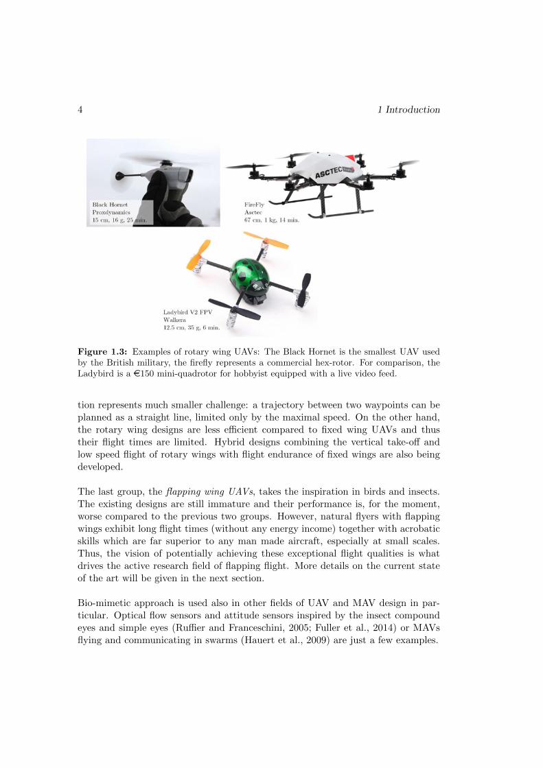
Rotary wing UAVs generate the lift by one or several rotating bladed rotors. Nowa-days, four and more rotor designs, known as quadrocopters and multicopters, arethe most popular UAV platform. These designs are inherently unstable and requirean on-board autopilot for attitude control. This, however, makes the designs alsovery manoeuvrable and agile yet relatively insensitive to disturbances. Nevertheless,the smallest commercially available professional MAV, the Black Hornet by Prox-dynamics, uses a traditional helicopter design with one main rotor and a stabilizingtail rotor. Examples of rotary wing UAVs are shown in Figure 1.3.
The advantage of rotary wing UAVs over fixed wing designs is the capability ofvertical take-off, hovering and slow flight in any direction, which makes them usefulespecially in confined urban environments or even indoors. Autonomous opera-
4 1 Introduction
Ladybird V2 FPV
Walkera
12.5 cm, 35 g, 6 min.
Figure 1.3: Examples of rotary wing UAVs: The Black Hornet is the smallest UAV usedby the British military, the firefly represents a commercial hex-rotor. For comparison, theLadybird is a e150 mini-quadrotor for hobbyist equipped with a live video feed.
tion represents much smaller challenge: a trajectory between two waypoints can beplanned as a straight line, limited only by the maximal speed. On the other hand,the rotary wing designs are less efficient compared to fixed wing UAVs and thustheir flight times are limited. Hybrid designs combining the vertical take-off andlow speed flight of rotary wings with flight endurance of fixed wings are also beingdeveloped.
The last group, the flapping wing UAVs, takes the inspiration in birds and insects.The existing designs are still immature and their performance is, for the moment,worse compared to the previous two groups. However, natural flyers with flappingwings exhibit long flight times (without any energy income) together with acrobaticskills which are far superior to any man made aircraft, especially at small scales.Thus, the vision of potentially achieving these exceptional flight qualities is whatdrives the active research field of flapping flight. More details on the current stateof the art will be given in the next section.
Bio-mimetic approach is used also in other fields of UAV and MAV design in par-ticular. Optical flow sensors and attitude sensors inspired by the insect compoundeyes and simple eyes (Ruffier and Franceschini, 2005; Fuller et al., 2014) or MAVsflying and communicating in swarms (Hauert et al., 2009) are just a few examples.

1.3 Flapping wing MAVs 5
1.3 Flapping wing MAVs
People have always been fascinated by flying animals. A sketch of one of the firstflying machines with flapping wings, although human powered, can be found inLeonardo da Vinci’s Paris Manuscript B dated 1488-1490 (Figure 1.4). However, ittook another five centuries to reach a sufficient technology level that allowed us tobuild first bio-inspired MAVs. The field of flapping wing MAVs is still very youngand provides plenty of space for improvement. The biggest challenge of flappingwing MAV design remains the integration of relatively complex flapping and controlmechanisms into a small and lightweight package that can be lifted by the thrustproduced.
Figure 1.4: Sketches of human powered flying machines with flapping wings by Leonardoda Vinci from Paris Manuscript B, 1488-1490.
1.3.1 Actuators and flapping mechanisms
When designing flying machines that mimic nature we need to find a replacementfor the animal’s powerful flight muscles as well as for their rapid metabolism sup-plying energy at high rates. Thanks to recent technological advancements in mobileelectronic devices, batteries with high energy densities emerged. Their high capac-ity to mass ratio made them a very attractive power source for MAVs. Thus, the

6 1 Introduction
Figure 1.5: Examples of flapping mechanisms. a) DelFly Micro mechanism (Bruggeman,2010), b)+c) Nano Hummingbird linkage and cable mechanism (Keennon et al., 2012), d)direct drive mechanism (Hines et al., 2014), e) compliant mechanism of Harvard robotic fly(Finio and Wood, 2010), f) flexible resonant wing (Vanneste et al., 2011), g) resonant thorax(Goosen et al., 2013).
majority of existing MAVs uses electric actuators driven by Lithium-ion (Li-ion) orLithium-ion polymer (Li-Pol) batteries.
The most common actuator is a DC motor, either with brushes (e.g. Keennon et al.,2012) or brushless (e.g. de Croon et al., 2009). It is usually combined with a reduc-tion gearbox and a transmission mechanism producing the flapping motion, whichcan either be a linkage mechanism as in Figures 1.5 a)+b) or a cable mechanism asin Figure 1.5 c). However, a direct drive option exploiting resonance is also beingexplored (Hines et al., 2014), see Figure 1.5 d).
Piezo-actuators are another option as they can be directly operated at the flappingfrequency. They are usually combined with a (compliant) linkage mechanism (Finioand Wood, 2010), Figure 1.5 e). Some flapping mechanisms try to mimic the res-

1.3 Flapping wing MAVs 7
onant thorax of insects, as this should provide high flapping amplitudes with lowenergy expenditure (Vanneste et al., 2011; Goosen et al., 2013). These designs aredriven by electro-magnetic actuators, see Figures 1.5 f)+g).
Apart from electric drives, an internal combustion engine was successfully used todrive a larger flapping wing MAV in the past (Zdunich et al., 2007). Also a ratherexotic chemical micro engine has been considered to drive a resonant thorax mech-anism (Meskers, 2010).
1.3.2 Tail stabilized and passively stable MAVs
The first designed flapping wing MAVs were either built passively stable, or usedtail surfaces for attitude stabilization. Majority of these designs have four wingsand take advantage of the clap-and-fling lift enhancement mechanism, which will beexplained in Section 2.3.2.
One of the first flapping wing MAVs was the Mentor shown in Figure 1.6 a), devel-oped under a DARPA program and presented in 2002. The first generation of thevehicle had a wingspan of 36 cm and weighted, from today’s perspective enormous,580 g due to an internal combustion engine driving the device. Nevertheless thevehicle was able to take-off and hover at a flapping frequency of 30 Hz. Two pairs ofwings were located at the top of the vehicle, flapping with 90 amplitude and usingthe clap-and-fling at both extremities. The flight was stabilized and actively con-trolled by fins exposed to the airflow coming from the wings. The flight endurancewas up to 6 minutes. The second generation used a brushless motor and was a bitsmaller and lighter (30 cm, 440 g). Its flight time was limited to only 20 s by thedischarge rate of the batteries available at that time.
DelFly was developed in 2005 by TU Delft (Lentink and Dickinson, 2009) and rep-resents one of many ornithopter projects (e.g. Park and Yoon, 2008; Yang et al.,2009). Unlike most ornithopters that fly only forward, the DelFly can also operatenear hovering or even fly slowly backwards, all controlled by tail control surfacesoperated by servos. Its two pairs of flapping wings are driven by a brushless motorand a linkage mechanism. It takes advantage of the clap-and-fling mechanism twice:when the lower wings meet the upper wings and also when the upper wings toucheach other. The current version, the DelFly Explorer shown in Figure 1.6 b), has awingspan of 28 cm, weights 20 g and has a flight endurance of 9 minutes (Wagteret al., 2014). It is capable of fully autonomous flight thanks to an on-board stereo-vision system (Tijmons et al., 2013). A smaller DelFly Micro shown in Figure 1.6 c)has a wingspan of 10 cm and weights only 3.07 g, including an on-board camera.

8 1 Introduction
Figure 1.6: Examples of flapping wing MAVs that are stabilized by tail or that are passivelystable.

1.3 Flapping wing MAVs 9
The first hovering passively stable MAV was built at Cornell University by vanBreugel et al. (2008), see Figure 1.6 e). It uses four pairs of wings, that clap andfling at both extremities. The vehicle has a 45 cm wingspan, although the wingsthemselves are rather short (around 85 mm). The flapping is driven by 4 DC pagermotors, one for each wing pair, and the total weight is 24.2 g. The passive stability isachieved by two lightweight sails, one above the wings and one at a greater distancebelow the wings. The vehicle can stay in the air, without any control, for 33 s. Anupdated version of the previous flyer, using only 2 wing pairs and a single motorwas presented by Richter and Lipson (2011). The major part of the robot, shownin Figure 1.6 f), is 3D printed, including the wings. With sails for passive stabilitythe robot weight is 3.89 g and it can fly for 85 s.
The last passively stable MAV has been presented recently by Ristroph and Chil-dress (2014). Unlike the previous robots, the inspiration comes from a swimmingjellyfish, see Figure 1.6 d). The vehicle has four wings, one on each side. The wingsdo not flap horizontally like in insects, but rather vertically. The opposing wingsflap together while the neighbouring wings are in anti-phase. The vehicle is verysmall (10 cm) and very light (2.1 g). It carries only a DC pager motor but no powersource; flying was demonstrated at 19 Hz flapping frequency while being tetheredto an external power source. The jelly-fish-like wings make the vehicle inherentlystable and thus it doesn’t need any additional stabilizing surfaces.
1.3.3 MAVs controlled by wing motion
Compared to the majority of MAVs from the previous section, designs that arestabilized and controlled by adjusting the wing motion are much closer in functionto their biological counterparts, insects and hummingbirds. However, they are alsomore complex because of the necessary control mechanisms that modify the wingkinematics. First MAV stabilized and controlled through wing motion was presentedin 2011 and only three designs have demonstrated stable hovering flight so far.
The Nano Hummingbird shown in Figure 1.7 a) is an MAV funded by DARPA,presented in 2011 by AeroVironment, mimicking a hummingbird (Keennon et al.,2012). It is the only flapping wing MAV capable of true hovering as well as of flightin any direction while carrying an on-board camera with live video feed. All thisis integrated into a robot with 16.5 cm wingspan weighting 19 g that has a flightendurance of up to 4 minutes. The necessary control moments are generated byindependent modulation of the wing twist.

10 1 Introduction
Figure 1.7: Examples of flapping wing MAVs that are actively controlled by wing motion.
The Harvard RoboBee with a wingspan of only 3 cm and weight of 80 mg is thesmallest and lightest MAV, see Figure 1.7 b). It took off for the first time in 2008while using guide wires for stabilization (Wood, 2008) and performed first controlledhovering flight five years later (Ma et al., 2013). It mimics insects of the Dipteraorder, the true flies. It has a single pair of wings that are driven independentlyby a pair of piezoelectric bimorph actuators. Each wing can be operated with dif-ferent amplitude, different mean position and different speed in each half-stroke,so that moments along the three body axis can be produced to stabilize the robotin air. The power source as well as flight controller remain off-board for the moment.
The BionicOpter, Figure 1.7 c), was built as a technology demonstrator of Festocompany (Festo, 2013). It mimics a dragonfly, although it is much larger (63 cmwingspan) and heavier (175 g). It uses four flapping wings that are driven by a singlemotor and that beat at a frequency of 15 Hz to 20 Hz. Their amplitude and flapping

1.4 Motivation and outline 11
plane inclination can be controlled independently by 8 servo motors in total, whichallows independent drag and lift modulation of each wing. Thus, the vehicle canhover as well as fly in any direction without the need to pitch or roll.
1.4 Motivation and outline
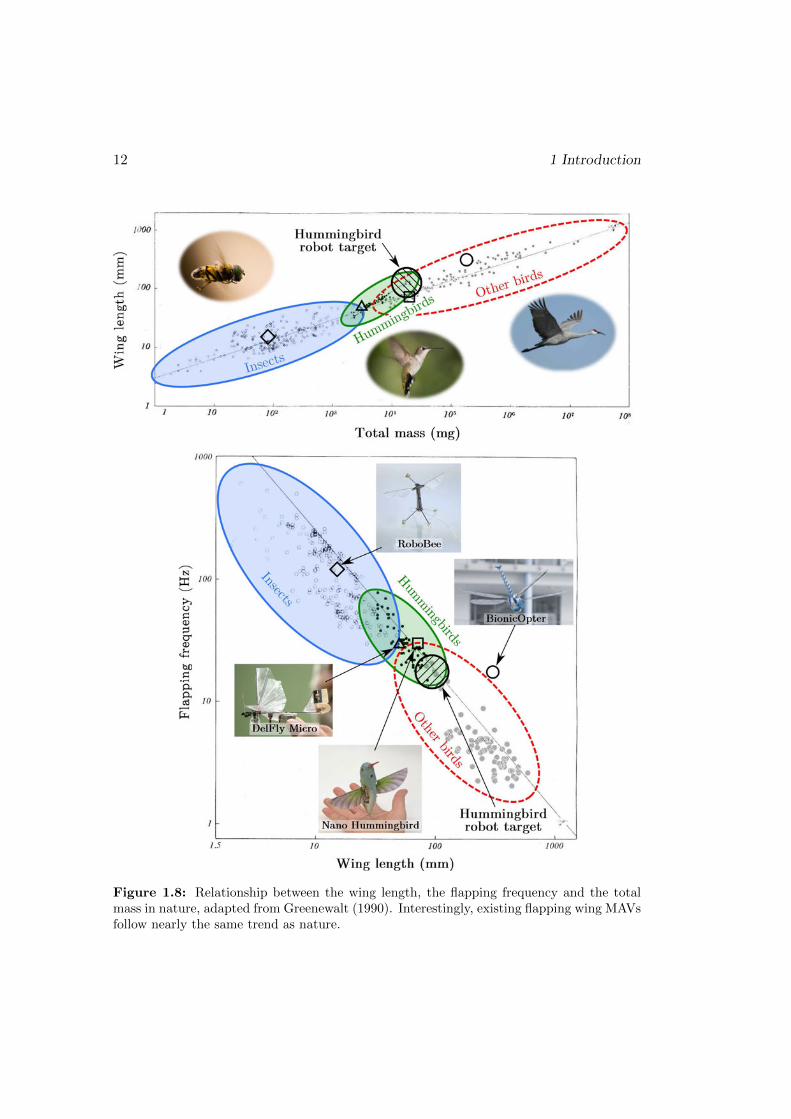
The goal of our project is to develop a tail-less flapping wing MAV capable of hov-ering flight. The flight should be stabilized and controlled by adapting the wingmotion. Looking into the nature, only insects and hummingbirds are capable of sus-tained hovering. Their wing beat frequency and total mass are linearly correlatedwith the wing length, see Figure 1.8. Interestingly, existing flapping wing MAVsalso follow this trend.
To make our lives easier, we have chosen to mimic larger hummingbirds, whichshould allow us to use, at least to some extent, some of the off-the-shelf componentsas well as traditional technologies. Thus, the target specification for the designedrobotic hummingbird was set to: 20 g total mass, 25 cm wingspan and flappingfrequency between 20 and 30 Hz.
The aim of this thesis is to design a working prototype of the wing motion controlmechanism that generates the control moments necessary to stabilize and controlthe flight. The thesis was split into two parts, theoretical (Chapters 2 - 5) andpractical (Chapters 6 - 7).
Chapter 2 recalls the basics of fixed wing aerodynamics. Then, different types offlight observed in nature are explained. More details are given on hovering flappingflight, its aerodynamic mechanisms as well as control mechanisms observed in nature.
Chapter 3 introduces a mathematical model of flapping flight, which combines quasi-steady aerodynamics and rigid body dynamics. Further, the model is linearised andreduced and its validity is demonstrated by comparisons to other models, includinga CFD study.
Chapter 4 is devoted to near-hover flapping flight stability. The damping effectscoming from the flapping wings are explained, with a special attention given to theeffect of wing position, and a simplified solution of the stability problem is proposed.
Chapter 5 describes the control design for the developed MAV, based on the lin-earised mathematical model. Wing kinematics parameters suitable for flight controlare identified and the control performance is demonstrated on numerical simulations.
12 1 Introduction
Figure 1.8: Relationship between the wing length, the flapping frequency and the totalmass in nature, adapted from Greenewalt (1990). Interestingly, existing flapping wing MAVsfollow nearly the same trend as nature.

1.5 References 13
Chapter 6 gives details on the development of the flapping mechanism and of thewing shape and presents experimental results obtained with a high speed cameraand a custom built force balance.
Finally, Chapter 7 describes the development of two control mechanisms and theirimplementation to the robot prototype. Their performance is demonstrated byforce and moment measurements and by high speed camera wing kinematics mea-surements.
1.5 References
B. Bruggeman. Improving flight performance of delfly ii in hover by improving wingdesign and driving mechanism. Master’s thesis, Delft University of Technology,2010.
G. de Croon, K. de Clerq, R. Ruijsink, B. Remes, and C. de Wagter. Design,aerodynamics, and vision-based control of the DelFly. International Journal ofMicro Air Vehicles, 1(2):71–97, Jun. 2009. doi:10.1260/175682909789498288.
Festo. BionicOpter. http://www.festo.com/cms/en_corp/13165.htm, 2013. Ac-cessed: 18/08/2014.
B. M. Finio and R. J. Wood. Distributed power and control actuation in the thoracicmechanics of a robotic insect. Bioinspiration & biomimetics, 5(4):045006, 2010.doi:10.1088/1748-3182/5/4/045006.
S. B. Fuller, M. Karpelson, A. Censi, K. Y. Ma, and R. J. Wood. Controlling freeflight of a robotic fly using an onboard vision sensor inspired by insect ocelli.Journal of The Royal Society Interface, 11(97), 2014. doi:10.1098/rsif.2014.0281.
J. F. Goosen, H. J. Peters, Q. Wang, P. Tiso, and F. van Keulen. Resonance basedflapping wing micro air vehicle. In International Micro Air Vehicle Conferenceand Flight Competition (IMAV2013), Toulouse, France, September 17-20, page 8,2013.
C. H. Greenewalt. Hummingbirds. Dover Publications, 1990.
S. Hauert, J.-C. Zufferey, and D. Floreano. Evolved swarming without positioninginformation: anapplication in aerial communication relay. Autonomous Robots,26(1):21–32, 2009. ISSN 0929-5593. doi:10.1007/s10514-008-9104-9.
L. Hines, D. Campolo, and M. Sitti. Liftoff of a motor-driven, flapping-wing mi-croaerial vehicle capable of resonance. IEEE Transactions on Robotics, 30(1):220–231, 2014. doi:10.1109/TRO.2013.2280057.

14 References
M. T. Keennon, K. R. Klingebiel, H. Won, and A. Andriukov. Development ofthe nano hummingbird: A tailless flapping wing micro air vehicle. AIAA paper2012-0588, pages 1–24, 2012.
D. Lentink and M. H. Dickinson. Biofluiddynamic scaling of flapping, spinning andtranslating fins and wings. Journal of Experimental Biology, 212(16):2691–2704,2009. doi:10.1242/jeb.022251.
K. Y. Ma, P. Chirarattananon, S. B. Fuller, and R. J. Wood. Controlledflight of a biologically inspired, insect-scale robot. Science, 340:603–607, 2013.doi:10.1126/science.1231806.
A. Meskers. High energy density micro-actuation based on gas generation by meansof catalysis of liquid chemical energy. Master’s thesis, Delft University of Tech-nology, 2010.
J. H. Park and K.-J. Yoon. Designing a biomimetic ornithopter capable of sustainedand controlled flight. Journal of Bionic Engineering, 5(1):39–47, 2008.
C. Richter and H. Lipson. Untethered hovering flapping flight of a 3d-printed me-chanical insect. Artificial life, 17(2):73–86, 2011. doi:10.1162/ artl a 00020.
L. Ristroph and S. Childress. Stable hovering of a jellyfish-like flying machine. Jour-nal of The Royal Society Interface, 11(92):1–13, 2014. doi:10.1098/rsif.2013.0992.
F. Ruffier and N. Franceschini. Optic flow regulation: the key to aircraft au-tomatic guidance. Robotics and Autonomous Systems, 50(4):177–194, 2005.doi:10.1016/j.robot.2004.09.016.
S. Tijmons, G. Croon, B. Remes, C. Wagter, R. Ruijsink, E.-J. Kampen, and Q. Chu.Stereo vision based obstacle avoidance on flapping wing mavs. In Q. Chu, B. Mul-der, D. Choukroun, E.-J. Kampen, C. Visser, and G. Looye, editors, Advances inAerospace Guidance, Navigation and Control, pages 463–482. Springer Berlin Hei-delberg, 2013. doi:10.1007/978-3-642-38253-6 28.
F. van Breugel, W. Regan, and H. Lipson. From insects to machines. RoboticsAutomation Magazine, IEEE, 15(4):68–74, 2008. doi:10.1109/MRA.2008.929923.
T. Vanneste, A. Bontemps, X. Q. Bao, S. Grondel, J.-B. Paquet, and E. Cattan.Polymer-based flapping-wing robotic insects: Progresses in wing fabrication, con-ception and simulation. In ASME 2011 International Mechanical EngineeringCongress and Exposition, pages 771–778. American Society of Mechanical Engi-neers, 2011.

References 15
C. D. Wagter, S. Tijmons, B. Remes, and G. de Croon. Autonomous flight of a 20-gram flapping wing mav with a 4-gram onboard stereo vision system. Acceptedat ICRA 2014, 2014.
R. J. Wood. The first takeoff of a biologically inspired at-scale roboticinsect. IEEE Transactions on Robotics, 24(2):341–347, Apr. 2008.doi:10.1109/TRO.2008.916997.
L.-J. Yang, C.-K. Hsu, F.-Y. Hsiao, C.-K. Feng, and Y.-K. Shen. A micro-aerial-vehicle (mav) with figure-of-eight flapping induced by flexible wing frames. InConference proceedings of 47th AIAA Aerospace Science Meeting, Orlando, USA,5-8, Jan., 2009 (AIAA-2009-0875), page 14. 47th AIAA Aerospace Science Meet-ing, Orlando, USA, 2009.
P. Zdunich, D. Bilyk, M. MacMaster, D. Loewen, J. DeLaurier, R. Kornbluh, T. Low,S. Stanford, and D. Holeman. Development and testing of the Mentor flapping-wing micro air vehicle. Journal of Aircraft, 44(5):1701–1711, 2007.

16 References
Chapter 2
Flapping flight
This chapter introduces the reader to the problematic of flapping flight. Becausethe majority of man made aircraft uses fixed wings, basic concepts of fixed wingaerodynamics are reviewed first. Then, three flight types observed in nature (glid-ing, flapping and hovering flapping flight) are described. An extra attention is givento the hovering flapping flight and its aerodynamic mechanisms enhancing the liftproduction as well as to flight control in nature.
2.1 Fixed wing aerodynamics
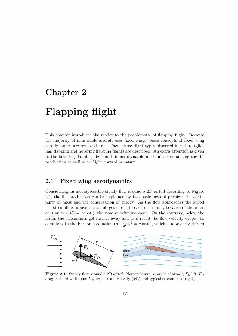
Considering an incompressible steady flow around a 2D airfoil according to Figure2.1, the lift production can be explained by two basic laws of physics: the conti-nuity of mass and the conservation of energy. As the flow approaches the airfoilthe streamlines above the airfoil get closer to each other and, because of the masscontinuity (AU = const.), the flow velocity increases. On the contrary, below theairfoil the streamlines get further away and as a result the flow velocity drops. Tocomply with the Bernoulli equation (p+ 1
2ρU2 = const.), which can be derived from
upper
lower
Figure 2.1: Steady flow around a 2D airfoil. Nomenclature: α angle of attack, FL lift, FDdrag, c chord width and U∞ free-stream velocity (left) and typical streamlines (right).
17

18 2 Flapping flight
the conservation of energy, the static pressure needs to drop above the wing and risebelow the wing. This pressure difference results in a suction force lifting the airfoil:the lift force.
Figure 2.2: Pressure distribution around an airfoil (left) and the resulting lift force distri-bution (right), from Whitford (1987).
The distribution of the lift force is given by the pressure distribution, as in Figure2.2. Thus, the resultant lift force vector is placed at the centre of pressure (CP).For an airfoil of a general shape, the CP location is varying with the angle of attack.However, it can be demonstrated by employing the thin airfoil theory that for asymmetric airfoil the CP lies in 1/4 of the chord from the leading edge.
If we start moving an airfoil from rest the flow pattern at the very beginning willlook like in Figure 2.3 (left). A circulation Γ will develop around the airfoil to fulfilthe Kutta condition, i.e. move the stagnation point to the trailing edge as in Figure2.3 (right). This circulation is associated to a vortex that remains bound to thewing and is thus called the bound vortex. According to Kelvin’s theorem, statingthat the total circulation is conserved, the bound vortex needs to be compensated
Figure 2.3: Circulation theory of lift: inviscid flow around an airfoil producing zero lift(left), circulation according to the Kutta condition (centre) and combined flow fulfilling theKutta condition and generating lift (right). Figure adapted from Ellington (1984c).

2.1 Fixed wing aerodynamics 19
by a vortex with an opposite circulation. This vortex is formed near the trailingedge due to high velocity gradients and is called the starting vortex. Once thetrailing edge is reached the flow reaches steady conditions: the bound vortex stopsgrowing and the starting vortex is shed into the wake. Similar transverse vortex isshed whenever the bound circulation changes, e.g. due to a change of angle of attack.
In a finite wing another pair of counter-rotating vortices is present in the wake be-hind the wing tips, one on each side. They are called the wing-tip vortices and arecaused by an opposite spanwise flow above and below the wing. The whole vortexsystem of a finite wing is shown in Figure 2.4. Stopping the wing suddenly makesalso the bound vortex shed, forming a ring vortex. It will be shown in the nextsection that similar vortex systems can be observed around flapping wings.
Figure 2.4: Vortex system of a finite span wing: a) Development of the starting vortexas the wing starts moving, b) steady state, c) vortex ring shed when the wing is stopped.Figure adapted from Lehmann (2004).
For a steady flow around a flat 2D airfoil the circulation of the bound vortex can beexpressed using the thin airfoil theory as
Γ = παcU∞, (2.1)
where α is the angle of attack, c the chord width and U∞ the free stream velocity.Combining the result with the Kutta-Joukowski theorem, F ′L = ρU∞Γ, we obtainthe lift force as
F ′L = ρU∞Γ = παcρU2∞, (2.2)
where ρ is the fluid density.

20 2 Flapping flight
The lift coefficient is a dimensionless characteristic of the airfoil profile defined as
CL =FL
12ρU
2∞S
=F ′L(1)
12ρU
2∞c(1)
, (2.3)
where S = c(1) is the surface of a unity span wing with a chord c. By combiningthe last two equations we obtain the lift coefficient for a flat airfoil as CL = 2πα.
According to equation (2.2) the lift of a theoretical flat airfoil increases linearly withangle of attack. In reality the lift drops above certain value of angle of attack, seeFigure 2.5. The pressure gradients on the upper airfoil side become too high, whichresults into flow separation due to viscosity. The pressure in the separated regiondoes not drop any more and as a consequence the lift is reduced. This phenomenonis called stall.
Figure 2.5: Stall: Lift coefficient drops at high angles of attack due to flow separation,from Whitford (1987).
While the lift force is given by the pressure distribution around the airfoil, there areseveral sources of drag force. The total drag of a 2D airfoil is called the profile drag.It is given by terms due to viscosity (skin friction drag) and due to pressure andsubsequent separation (form drag). The total drag coefficient is defined similarly tothe lift coefficient
CD =FD
12ρU
2∞S
=F ′D(1)
12ρU
2∞c(1)
. (2.4)
In a finite wing, a small downward flow component, called the downwash w, is su-perposed to the flow around the wing, coming from the wing tip vortices (Figure2.6). The downwash varies along the wingspan and as a result the local angle ofattack changes. The original, geometric, angle of attack αg decreases by an induced

2.2 Flight in nature 21
Figure 2.6: Wing tip vortices formed in clouds behind Boeing B-757 (left) and the effectsof the resulting downwash on a local section of a finite length wing (right).
angle of attack αi. The local lift is then produced according to an effective angle ofattack αeff = αg − αi measured with respect to the relative flow.
Since the local lift vector FL is perpendicular to the relative flow vector, it has acomponent in the direction of U∞ called the induced drag FDi. The induced dragincreases with increasing angle of attack. It is proportional to the inverse of thesquare of velocity and so it is mostly important at low speeds. The induced dragcan be reduced by several design means (high aspect ratio wing, tapered wing,twisted wing, winglets, ...).
2.2 Flight in nature
No matter how big progress has been made in aviation since the first powered flight ofthe Wright brothers in 1903, the flight qualities and agility of modern aircraft remainincomparable to flying animals that have evolved over several hundred millions ofyears. When looking into nature, three types of flight can be observed: gliding flight,flapping flight and hovering.
2.2.1 Gliding flight
In gliding flight the animal is moving forward and descending at the same time. Thenecessary thrust to maintain the forward speed is produced by the gravity force. Itis a common flight technique for bats and larger birds, but gliding flight was alsoobserved among certain fish, frogs, reptiles or even squirrels. The aerodynamics ofmost gliding animals can be described by the theory for fixed wing aircraft.
The ratio between the lift and drag is equal to the glide ratio, which relates the trav-elled horizontal distance to the vertical descent. The best natural gliders, vultures

22 2 Flapping flight
CLmax trailing-edge flap (a)
a
b
c
d
leading-edge slat (b)
split flap (d)
slotted trailing edge flap (c)
symmetric airfoil
Figure 2.7: High lift devices used in aircraft and their equivalents in flying animals, fromNorberg (2002).
and albatrosses, can achieve glide ratios higher than 20:1 (Pennycuick, 1971). Forcomparison, the best man made glider has a glide ratio of 70:1 (Flugtechnik & Le-ichtbau, 2001). To keep the altitude some animals glide in ascending air that risesdue to convenient atmospheric conditions or due to terrain relief. Such flight iscalled soaring.
Several mechanisms are used to increase the maximal lift coefficient of fixed wingaircraft. These high lift devices, consisting of flaps and slats, are used particularly atlow flight speeds, i.e. during take-off and landing, see Figure 2.7 (top). Equivalentmechanisms can be observed in natural flyers (Norberg, 2002). Bats can activelycontrol the camber of their wing (Figure 2.7 a), which increases the lift coefficientand delays the stall. It is equivalent to trailing edge flaps and Kreuger flaps ordrooped leading edges used in aircraft. Stall can be further delayed by leading-edgeslats and slotted trailing edge flaps. The role of these devices, which deviate partof the flow from below the wing above the wing, is to delay the stall by modifyingthe pressure distribution above the wing and energizing the upper surface boundary

2.2 Flight in nature 23
layer. Birds can achieve similar effect by lifting their “thumb” with several featherson the leading edge (Figure 2.7 b). Equivalent to the slotted trailing edge flaps canbe observed in birds with long forked tail, which they can spread wide to help keep-ing the flow attached even at high angles of attack (Figure 2.7 c). During landings,a raised covert feathers can be observed in many birds (Figure 2.7 d). This self-activated mechanism prevents backward flow of the turbulent air and delays flowseparation. It is similar to split flaps, used during aircraft landings to increase thegliding angle.
Vortex generators in Sea Harrier
Wikimedia Commons, commons.wikimedia.org
de.academic.ru
a) Protruding digit in a bat wing
b) Serrated leading edge feather of an owl
c) Corrugated dragonfly wing
Figure 2.8: Vortex generators used in aircraft to introduce turbulence into the boundarylayer (left) and their equivalents in flying animals, from Norberg (2002); Neuweiler (2000),(right).
Another way to delay the stall is to introduce turbulence in the boundary layer of theupper wing surface. The turbulence helps to maintain an interchange of momentumbetween the slow layers close to the wing and the free flow, so the flow separationoccurs at higher angles of attack. In aircraft, this is done by vortex generators, whichare typically placed close to the thickest part of the wing and distributed along thespan, see Figure 2.8 (left). A protruded digit on bat wing, serrated feathers at thewing leading edge in owls and corrugated wings of dragonflies have the same role,see Figure 2.8 (right). Apart from delaying the stall, this solution also reduces theflight noise.
24 2 Flapping flight
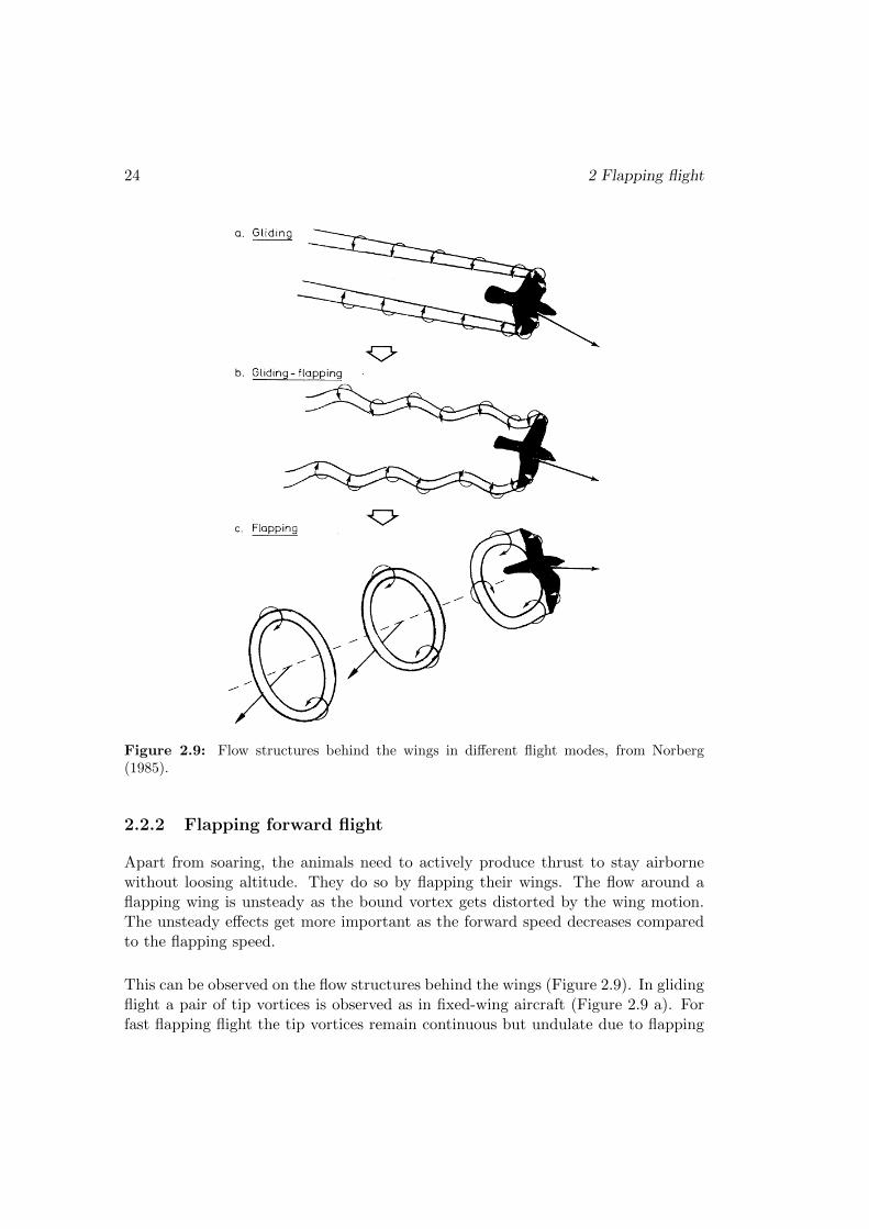
Figure 2.9: Flow structures behind the wings in different flight modes, from Norberg(1985).
2.2.2 Flapping forward flight
Apart from soaring, the animals need to actively produce thrust to stay airbornewithout loosing altitude. They do so by flapping their wings. The flow around aflapping wing is unsteady as the bound vortex gets distorted by the wing motion.The unsteady effects get more important as the forward speed decreases comparedto the flapping speed.
This can be observed on the flow structures behind the wings (Figure 2.9). In glidingflight a pair of tip vortices is observed as in fixed-wing aircraft (Figure 2.9 a). Forfast flapping flight the tip vortices remain continuous but undulate due to flapping

2.2 Flight in nature 25
(Figure 2.9 b). For slower speeds the downstroke becomes dominant in thrust gener-ation. Transverse vortices are being periodically created on the trailing edge at thebeginning and at the end of each downstroke (Shyy et al., 2013). It is similar to thestarting vortex and to the shedding of bound vortex when a fixed wing starts andstops to move, respectively. These transverse vortices connect with the two wing tipvortices and a vortex ring is shed at the end of each downstroke (Figure 2.9 c).
With decreasing flight speed the animals adapt the flapping motion direction. Theflapping plane is almost vertical for cruising speeds but it inclines backwards as thespeed decreases (Figure 2.10). The body posture is also adapted.
6 m s–1 14 m s–110 m s–1 12 m s–18 m s–1
Figure 2.10: Wing-tip path of a pigeon flying at speeds of 6-14 m.s-1. Adapted fromTobalske and Dial (1996).
2.2.3 Hovering flight
Hovering flight can be mostly observed in insects and hummingbirds. While bats(Muijres et al., 2008) and other birds (Tobalske et al., 1999) are also capable ofhovering, they only use it in transitions (taking off, landing, perching) as hoveringcan require more than twice the power necessary for cruising (Dial et al., 1997).Apart from hummingbirds, birds generate most of the lift during downstroke whentheir wing is fully extended; they flex their wings in upstroke to reduce drag (Figure2.11). We call this type of hovering asymmetric hovering (Norberg, 2002) or avianstroke (Azuma, 2006).
Hummingbirds and many insects can hover for much longer periods as they usesymmetric hovering, also called insect stroke (Figures 2.12). The wings remain fullyextended throughout the wingbeat, but rotate and twist at the end of each halfstroke. Hummingbirds flap their wings almost horizontally (Figure 2.13 left) andproduce lift also during upstroke, about 25%-33%. The flapping plane of two-wingedinsects can be slightly inclined (Figure 2.13 right); nevertheless, the upstroke gener-ates up to 50% (Warrick et al., 2005, 2012).

26 2 Flapping flight
Downstroke
Upstroke
Time
Figure 2.11: Asymmetric hovering typical for birds and bats. Adapted from Azuma (2006).
Downstroke
Upstroke
Time
Figure 2.12: Symmetric hovering typical for hummingbirds (left) and insects (right).Adapted from Greenewalt (1990).
Figure 2.13: Wingtip trajectory in hovering hummingbirds and insects. Adapted fromEllington (1984a,b).

2.2 Flight in nature 27
Hummingbird wing morphology differs from other birds as the the upper arm andforearm bones are significantly shorter (Figure 2.14) and so the “hand” part of thewing, called the handwing, is much larger: over 75% of wing area in hummingbirdscompared to about 50% in most birds (Warrick et al., 2012). On top of that thewrist and the elbow cannot articulate; all the motion comes from the very mobileshoulder. The wing is being moved by a pair of powerful muscles: a depressor mus-cle powers the downstroke and an elevator the upstroke. The depressor is twiceas heavy as the elevator, which corresponds to the uneven lift production betweendownstroke and upstroke mentioned earlier. The hummingbird muscles form up to30% of the body weight (Greenewalt, 1990, p116).
Figure 2.14: Wing morphology: size of forelimb bones with human arm as a reference(left) and handwing size (right, handwing in grey). The handwing is significantly larger inhummingbirds. Adapted from Dial (1992); Warrick et al. (2012) and www.aokainc.com.
There are two ways how flapping motion is produced in insects (Dudley, 2002). Phy-logenetically older insects use direct muscles to flap their wings (Figure 2.15 left).They have two groups of muscles, the depressors and the elevators, that contract tomove the wing in downstroke and in upstroke, respectively. Direct drive is typicalfor four-winged insects like dragonflies and damselflies. The brain controls each wingindependently, which makes their flight very agile, but it also limits their flappingfrequency, which is relatively low.
In phylogenetically modern insects, e.g. flies and bees, the wings are driven indi-rectly by the deformation of thorax and by displacing the dorsal part of the thoraxcalled the notum (Figure 2.15 right). The upstroke is effected by contracting thevertical muscles and lowering the notum. Longitudinal muscles are contracted indownstroke to deform the thorax in longitudinal direction and subsequently raisethe notum. The thorax acts as a resonant system, so the animals can flap at muchhigher frequencies, with greater amplitudes and the wings are always synchronized.

28 2 Flapping flight
Figure 2.15: Direct (left) and indirect insect flight muscles (right). From Hill et al. (2012).
Surprisingly, the maximum lift to muscle-weight ratio is constant among insects andbirds, despite their different evolution paths (Marden, 1987).
Hummingbirds and insects can combine precise hovering flight with fast cruising aswell as with backward flight. Figure 2.16 shows wing-tip path and body positionsof a hummingbird in all the mentioned flight modes. As in other birds, the flappingplane is nearly vertical in cruising. It inclines backwards as the flight speed de-creases becoming approximately horizontal when hovering. It inclines further backto fly backwards. The wing-tip follows an oval pattern in most situations, but afigure-of-eight pattern is used near hovering.
Figure 2.17 shows wing-tip paths of a bumblebee flying at different speeds. Thepaths in this figure combine the flapping velocity with the downwash (the air movedby the interaction with the flapping wings). The shape of these paths can be charac-terized by a dimensionless ratio between the flight velocity and the (average) flappingvelocity called the advance ratio (Ellington, 1984b)
J =U
2ΦfR, (2.5)

2.2 Flight in nature 29
Figure 2.16: Wing-tip paths of a hummingbird in forward, hovering and backward flight.Adapted from Greenewalt (1990).
Figure 2.17: Wing-tip paths of a bumblebee at different flight speeds composed of flappingvelocity and downwash. The arrows represent the generated forces. The imbalance betweenupstroke and downstroke path lengths and forces is characterized by the advance ratio J .Figure from Ellington (1999).

30 2 Flapping flight
where Φ is the flapping amplitude, f the flapping frequency and R the wing length.Ellington defines hovering as flight with advance ratio J below 0.1, where both up-stroke and downstroke produce approximately equal amount of lift. We can observethat as the advance ratio increases, the upstroke paths become more vertical andshorter while downstroke paths more horizontal and longer. This signifies that forhigher advance ratios downstroke generates higher force, which is directed upwardsto provide lift, while the force during upstroke is smaller and is directed forwards toprovide thrust.
2.3 Hovering flapping flight aerodynamics
Because of the scope of this work, only symmetric hovering flight (ie. flight withan advanced ratio J less than 0.1) with a single pair of flapping wings is consideredfurther.
2.3.1 Dynamic scaling
The flow patterns over flapping wings can be characterized by several dimensionlessnumbers (Shyy et al., 2013). The most important is the Reynolds number whichrelates the inertial and viscous forces. For hovering flight it is defined as
Rehover =UrefLref
ν=
2ΦfRc
ν=
4ΦfR2
νA, (2.6)
where ν is the kinematic viscosity of air, the mean tip velocity, calculated as 2ΦfR,is taken as the reference speed Uref and mean chord c as the reference length Lref .The definition was also rewritten using the wing aspect ratio A = 2R
c . We can seethat for flyers with similar flapping amplitudes Φ and aspect ratiosA the Reynoldsnumber is proportional to fR2. Typical Reynolds numbers for hovering flappingflight lie between ∼10 and ∼10 000.
For forward flight the forward velocity U∞ is usually taken as the reference velocityand the definition becomes independent of flapping
Reforward =U∞c
ν. (2.7)
Another dimensionless quantity, characterizing an oscillating flow, is the Strouhalnumber. It relates the oscillatory and forward motion and is thus only applicable toforward flight. It is defined as
St =fLrefUref
=ΦfR
U∞, (2.8)

2.3 Hovering flapping flight aerodynamics 31
where the reference length is the distance travelled by the wing tip over one half-stroke ΦR. The Strouhal numbers typical for most swimming and flying animalsare between 0.2 and 0.4 (Taylor et al., 2003).
The level of unsteadiness associated with flapping wings in hover can be character-ized by the reduced frequency used for pitching and plunging airfoils. It is definedas
khover =2πfLrefUref
=πfc
2ΦfR=
π
ΦA, (2.9)
where the reference velocity is again the mean tip velocity and the reference length ishalf of the mean chord c/2. The higher is the value of reduced frequency the greateris the role of the unsteady effects on the aerodynamic force production. Morpholog-ical data and dimensionless numbers of several hovering animals are in Table 2.1.
Chalcid FruitHawkmoth
Rufous Giantwasp fly hummingbird hummingbird
m [g] 2.6e-7 0.002 1.6 3.4 20R [mm] 0.7 2.39 48.3 47 130c [mm] 0.33 0.78 18.3 12 43f [Hz] 370 218 26.1 43 15Φ [] 120 140 115 116 120A [-] 4.2 6.1 5.3 7.8 6Re [-] 23 126 5885 6249 22353k [-] 0.35 0.21 0.30 0.20 0.25
Table 2.1: Morphological parameters and dimensionless numbers of hovering flapping flightin nature. Data taken from Shyy et al. (2010); Weis-Fogh (1973).
2.3.2 Lift enhancing aerodynamic mechanisms
When researchers tried to model insect aerodynamics using traditional, steady stateformulations in a quasi steady manner the models would grossly under-predict thegenerated lift; some of the animals would hardly be able to take-off (Ellington,1984a). This induced further research that revealed that the produced forces are en-hanced by flow patterns of highly unsteady nature. The flow structures around thewings involve periodic formation and shedding of vortices; they are still under activeresearch. Many key mechanisms were observed and identified both experimentallyand numerically, including the delayed stall of leading edge vortex, Kramer effect,wake capture and clap-and-fling (Sane, 2003; Lehmann, 2004).
32 2 Flapping flight
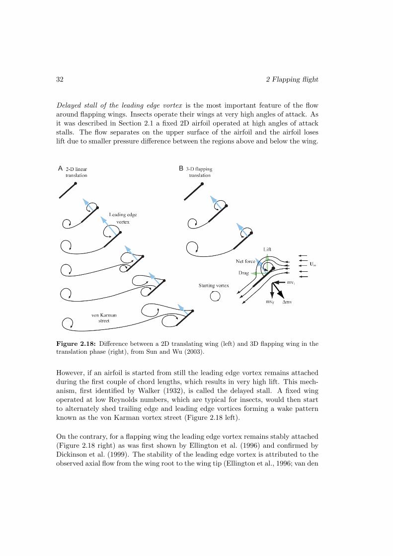
Delayed stall of the leading edge vortex is the most important feature of the flowaround flapping wings. Insects operate their wings at very high angles of attack. Asit was described in Section 2.1 a fixed 2D airfoil operated at high angles of attackstalls. The flow separates on the upper surface of the airfoil and the airfoil loseslift due to smaller pressure difference between the regions above and below the wing.
Figure 2.18: Difference between a 2D translating wing (left) and 3D flapping wing in thetranslation phase (right), from Sun and Wu (2003).
However, if an airfoil is started from still the leading edge vortex remains attachedduring the first couple of chord lengths, which results in very high lift. This mech-anism, first identified by Walker (1932), is called the delayed stall. A fixed wingoperated at low Reynolds numbers, which are typical for insects, would then startto alternately shed trailing edge and leading edge vortices forming a wake patternknown as the von Karman vortex street (Figure 2.18 left).
On the contrary, for a flapping wing the leading edge vortex remains stably attached(Figure 2.18 right) as was first shown by Ellington et al. (1996) and confirmed byDickinson et al. (1999). The stability of the leading edge vortex is attributed to theobserved axial flow from the wing root to the wing tip (Ellington et al., 1996; van den

2.3 Hovering flapping flight aerodynamics 33
Figure 2.19: Leading edge vortex stabilized by axial flow, from van den Berg and Ellington(1997)
Berg and Ellington, 1997; Usherwood and Ellington, 2002), see Figure 2.19, similarlyto low aspect ratio delta wings. This flow tends to be important for higher Reynoldsnumbers, while being rather weak for lower Reynolds numbers (Birch et al., 2004),nevertheless this seems to be sufficient for the leading edge vortex stability (Shyyand Liu, 2007).
The leading edge vortex enhances not only the lift but also the drag force. It con-tributes by about 7 to 16% to the bound circulation of a hummingbird wing (Warricket al., 2009) and by up to 40% to the circulation of slow flying bats (Muijres et al.,2008).
The second mechanism that can enhance the lift production is the Kramer effect,sometimes called the rapid pitch rotation (Shyy et al., 2010) or rotational forces(Sane and Dickinson, 2002). As it was first demonstrated by Kramer (1932) in thecontext of wing flutter, the lift of a fixed wing in steady flow will increase if thewing rotates from low to high angle of attack. The span-wise rotation of the wingcauses that the stagnation point moves away from the trailing edge and as a resultadditional circulation is generated to restore the Kutta condition. Depending on thesense of rotation, this circulation is added to or subtracted from the bound vortexcirculation which results into positive or negative change of lift force, respectively.

34 2 Flapping flight
Similar mechanism occurs in flapping wings at the reversal point between strokes,where the wing rotates rapidly along its span-wise axis. Studies of this phenomenacarried out by Dickinson et al. (1999); Sane and Dickinson (2002) showed that anadvanced rotation will enhance the lift force whereas a delayed rotation will causethe lift to drop. Insects take advantage of this phenomena by timing the rotationduring manoeuvres (Dickinson et al., 1993).
Another mechanism related to the stroke reversal is the wake capture, sometimesalso called the wing-wake interaction. It was first demonstrated by Dickinson et al.(1999) and further investigated by Birch and Dickinson (2003). As the wing reversesit interacts with the shed vortices from the previous strokes (Figure 2.20). Thisincreases the relative flow speed and the transferred momentum results in higheraerodynamic force just after reversal. The magnitude of this enhancement dependsstrongly on the wing kinematics just before and just after the reversal.
Figure 2.20: Wake capture mechanism. Light blue arrows represent the generated force,dark blue arrows show the flow direction, from Sane (2003)
The last aerodynamic mechanism enhancing the lift is called the clap-and-fling orclap-and-peel (Weis-Fogh, 1973; Ellington, 1984b). It occurs only in animals thattouch their wings dorsally at the end of upstroke. In the ’clap’ phase the wings touchfirst with their leading edges and keep rotating until also the trailing edges touch,pushing the trapped air downwards, which generates additional thrust (Figure 2.21).Once the wings start to ’fling’ apart a gap opens between the leading edges. The airis sucked in which boosts the circulation build-up around the wings. Also, the start-ing vortices eliminate each other which further enhances the circulation development.
Clap-and-fling mechanism was observed in multiple insect species (e.g. Weis-Fogh(1973); Ellington (1984b); Zanker (1990)) and can enhance the lift by up to 25%(Marden, 1987).

2.3 Hovering flapping flight aerodynamics 35
Figure 2.21: Clap and fling mechanism. Light blue arrows represent the generated force,dark blue arrows show the flow direction, from Sane (2003).
Apart from purely aerodynamic mechanisms, the interaction of the flow and thewing structure can also have a positive effect on the lift production (Shyy et al.,2013; Tanaka et al., 2013). For example, an appropriate combination of chord- andspan-wise flexibility leads to a relative phase-advance of the wing rotation, resultinginto lift increase due to Kramer effect.
2.3.3 Flight stability
While lift generation is of a primary importance for flying animals they also need tobalance their body when facing perturbations coming from the wind or when ma-noeuvring. Many works tried to identify whether this stability is inherent or whetherit is augmented by the sensory systems. To control the flight, insects can rely ontheir vision (compound eyes and ocelli) as well as on airflow sensors (antennae andwind sensitive hairs) and on inertial sensors (halteres), see Taylor and Krapp (2008).Studying passive stability experimentally is complicated as breaking the feedbackloops by “deactivation” of the sensory systems leads to abnormal behaviour of theanimal. Thus, numerical treatment was preferred by most authors.
36 2 Flapping flight
The numerical studies employed aerodynamic models with various complexities(CFD, quasi-steady aerodynamics). The studies considered hovering or forwardflight and covered both longitudinal and lateral directions of various insect speciesdiffering in size and in wing kinematics (Sun et al., 2007; Xiong and Sun, 2008;Zhang and Sun, 2010; Faruque and Humbert, 2010a,b; Orlowski and Girard, 2011;Cheng and Deng, 2011). While minor differences in the predicted behaviour existespecially in the lateral direction (Karasek and Preumont, 2012), the common con-clusion is that the hovering flapping flight is inherently unstable and needs to beactively controlled.
Experimental studies of near-hover flapping flight stability are sparse. Taylor andThomas (2003) performed experiments on a desert locust in forward flight and foundthat it was unstable. However, the animal was tethered and it could use its sensorysystems. Hedrick et al. (2009) studied yaw turns in animals ranging from fruit fliesto large birds. They showed that the deceleration phase of a yaw turn can be ac-complished passively, without any active control of the animal, thanks to dampingcoming from the flapping motion, which they termed Flapping Counter Torque.
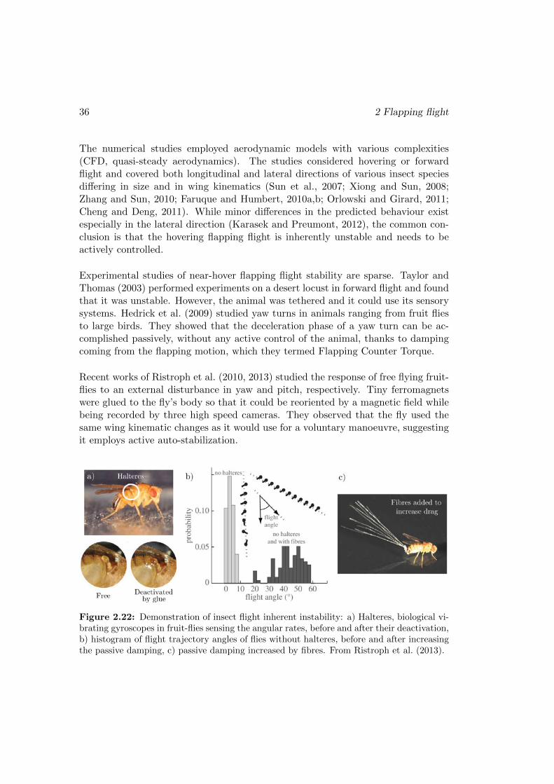
Recent works of Ristroph et al. (2010, 2013) studied the response of free flying fruit-flies to an external disturbance in yaw and pitch, respectively. Tiny ferromagnetswere glued to the fly’s body so that it could be reoriented by a magnetic field whilebeing recorded by three high speed cameras. They observed that the fly used thesame wing kinematic changes as it would use for a voluntary manoeuvre, suggestingit employs active auto-stabilization.
Figure 2.22: Demonstration of insect flight inherent instability: a) Halteres, biological vi-brating gyroscopes in fruit-flies sensing the angular rates, before and after their deactivation,b) histogram of flight trajectory angles of flies without halteres, before and after increasingthe passive damping, c) passive damping increased by fibres. From Ristroph et al. (2013).

2.3 Hovering flapping flight aerodynamics 37
In the next experiment they deactivated the halteres (insect gyroscopes), leavingthe fly with only the visual feedback, whose reaction is about four times slower.This made the fly unable to fly as it fell nearly straight down, suggesting that theflight is indeed inherently unstable. Nevertheless, it was possible to restore theinsects stability by attaching light dandelion fibres to its abdomen. This generatedsufficient damping, so that the insect could keep more or less the same orientation,see Figure 2.22.
2.3.4 Attitude stabilization
Due to the inherent instability of flapping flight, hovering animals need to balancetheir bodies actively. The attitude stabilization requires independent control of bodyrotation around the roll (longitudinal) and pitch (lateral) axis. On top of that, turn-ing requires control of rotation around the yaw (vertical) body axis. The necessarymoments are produced by introducing small asymmetries into otherwise symmetricwing motion.
Figure 2.23: Pitch moment generation in insects: a) via angle of attack asymmetry, b) viamean wing position. Adapted from Conn et al. (2011).
For pitching the animal needs to shift the centre of lift in fore/aft direction (Elling-ton, 1999). This shift can be realized by moving the maximal/minimal wing strokepositions (the mean stroke angle) and/or by a difference in the angle of attack duringupstroke and downstroke (Dudley, 2002), see Figure 2.23. The former was observedin free flying fruit flies during the auto-stabilization after an externally triggeredpitch perturbation (Ristroph et al., 2013) and also in tethered fruit flies (Zanker,1988).

38 2 Flapping flight
Figure 2.24: Roll moment generation in insects: a) via angle of attack difference, b) viaflapping amplitude difference. Adapted from Conn et al. (2011).
Roll can be initiated by introducing an asymmetry between the lift of the left andright wing. Insects achieve this by increasing the flapping amplitude and/or bymodifying the angle of attack on one wing (Ellington, 1999), as it was observed intethered fruit-flyes (Hengstenberg et al., 1986), see Figure 2.24.
Finally yawing can be effected by increasing the drag force on one of the wings. Adifference in angle of attack while yawing was observed by Ellington (1999), see Fig-ure 2.25. The same was reported for fruitflies by Bergou et al. (2010), together withsignificant asymmetry of mean stroke angles. Nevertheless, they attributed 98% ofthe yaw moment to the angle of attack difference. Interestingly, a different strategyin fruit-fly yaw turns was reported by Fry et al. (2003). They observed a backwardtilt of stroke plane together with an increase of amplitude on the outside wing.
Figure 2.25: Yaw moment generation in insects via angle of attack asymmetry. Adaptedfrom Conn et al. (2011).

2.3 Hovering flapping flight aerodynamics 39
Apart from wings also other body parts contribute to the overall torques produced.Zanker (1988) observed lateral deflection of the abdomen that should increase thedrag on one side during visually simulated yaw turns in tethered fruit-flies. A(smaller) dorso-ventral deflection was reported while pitching. The drag can beincreased further by hindlegs (Zanker et al., 1991). Video footages of flying hum-mingbirds also reveal that many species use their tail, in addition to wing motionand stroke plane changes, to control their body rotation when manoeuvring, seeFigure 2.26.
Figure 2.26: Rufous hummingbird flying backwards. The interval between the dis-played positions is 3 wingbeats, each position is a composite of two frames to showthe wing limit positions and the stroke plane direction. Original video footage,http://youtu.be/Cly6Y69WOYk, courtesy of JCM Digital Imaging (http://jcmdi.com).

40 References
2.3.5 Flight control
Flying animals control their speed by modulating the thrust force. Hummingbirdscan increase the produced thrust by increasing the stroke amplitude and at a smallerrate also the flapping frequency, as it was documented by Altshuler and Dudley(2003) by load lifting. The same was observed by Chai et al. (1996) by reducingthe air pressure. Insects on the other hand are operating their wings at an approxi-mately constant frequency (Dudley, 2002), because their thorax works as a resonantsystem. The thrust modulation is thus achieved through changes of flapping ampli-tude. Some insects can however further enhance the thrust by employing the clapand fling mechanism (Ellington, 1999), which can provide an additional boost of upto 25% (Marden, 1987). The maximal amplitudes of both hummingbirds and insectsare mechanically limited by their morphology.
Flying forward and sideways is usually achieved by tilting the mean thrust vectorinto the desired direction, resulting into a horizontal force component that acceler-ates the flight. This strategy is similar to helicopters. In steady flight, the animalsdo this by tilting the stroke plane together with the body along the pitch or alongthe roll axis for forward/backward or sideways flight respectively (Vogel, 1967; Dud-ley and Ellington, 1990; Dudley, 2002; Tobalske et al., 2007). However, the relativeangle between the body axis and stroke plane can slightly change when manoeu-vring, see Figure 2.26. The same was observed in hawkmoths even in steady flight(Willmott and Ellington, 1997).
A strategy that generates directly a longitudinal or lateral force by modulatingthe drag forces was observed recently. Forward flight was induced by a paddlingmotion in fruit-fly (Ristroph et al., 2011), as the fly used different angles of attackduring upstroke and downstroke. A lateral force resulting into sideways flight canbe generated by differential timing of wing rotation in the same species (Ristrophet al., 2009).
2.4 References
D. L. Altshuler and R. Dudley. Kinematics of hovering hummingbird flight alongsimulated and natural elevational gradients. Journal of Experimental Biology, 206:3139–3147, 2003. doi:10.1242/jeb.00540.
A. Azuma. The Biokinetics of Flying and Swimming. AIAA Education Series. AIAA,2nd edition edition, 2006.

References 41
A. J. Bergou, L. Ristroph, J. Guckenheimer, I. Cohen, and Z. J. Wang. Fruit fliesmodulate passive wing pitching to generate in-flight turns. Physical review letters,104(14):1–4, 2010. doi:10.1103/PhysRevLett.104.148101.
J. M. Birch and M. H. Dickinson. The influence of wingwake interactions on the pro-duction of aerodynamic forces in flapping flight. Journal of Experimental Biology,206:2257–2272, 2003. doi:10.1242/jeb.00381.
J. M. Birch, W. B. Dickson, and M. H. Dickinson. Force production andflow structure of the leading edge vortex on flapping wings at high and lowreynolds numbers. Journal of Experimental Biology, 207:1063–1072, 2004.doi:10.1242/jeb.00848.
P. Chai, R. Harrykissoon, and R. Dudley. Hummingbird hovering performance inhyperoxic helliox: effects of body mass and sex. Journal of Experimental Biology,199:2745–2755, 1996.
B. Cheng and X. Deng. Translational and rotational damping of flapping flight andits dynamics and stability at hovering. IEEE Transactions on Robotics, 27(5):849–864, Oct. 2011. doi:10.1109/TRO.2011.2156170.
A. T. Conn, C. S. Ling, and S. C. Burgess. Biomimetic analysis of insect wingkinematics for flapping MAVs. International Journal of Micro Air Vehicles, 3(1):1–11, 2011. doi:10.1260/1756-8293.3.1.1.
K. Dial, A. Biewener, B. Tobalske, and D. Warrick. Mechanical power output ofbird flight. Nature, 390(6655):67–70, 1997.
K. P. Dial. Avian forelimb muscles and nonsteady flight: Can birds fly without usingthe muscles in their wings? The Auk, 109(4):874–885, 1992.
M. H. Dickinson, F.-O. Lehmann, and K. G. Gtz. The active control of wing rotationby drosophila. Journal of Experimental Biology, 182:173–189, 1993.
M. H. Dickinson, F.-O. Lehmann, and S. P. Sane. Wing rotation and theaerodynamic basis of insect flight. Science, 284(5422):1954–1960, Jun. 1999.doi:10.1126/science.284.5422.1954.
R. Dudley. The Biomechanics Of Insect Flight: Form, Function, Evolution. Prince-ton University Press, 2002.
R. Dudley and C. P. Ellington. Mechanics of forward flight in bumblebees: I. kine-matics and morphology. Journal of Experimental Biology, 148(1):19–52, 1990.

42 References
C. P. Ellington. The aerodynamics of hovering insect flight. I. the quasi-steadyanalysis. Philosophical Transactions of the Royal Society of London. Series B,Biological Sciences, 305(1122):1–15, Feb. 1984a.
C. P. Ellington. The aerodynamics of hovering insect flight. III. kinematics. Philo-sophical Transactions of the Royal Society of London. Series B, Biological Sci-ences, 305(1122):41–78, Feb. 1984b.
C. P. Ellington. The aerodynamics of hovering insect flight. IV. aerodynamic mech-anisms. Philosophical Transactions of the Royal Society of London. Series B,Biological Sciences, 305(1122):79–113, Feb. 1984c.
C. P. Ellington. The novel aerodynamics of insect flight: application to micro-airvehicles. Journal of Experimental Biology, 202:3439–3448, 1999.
C. P. Ellington, C. van den Berg, A. P. Willmott, and A. L. R. Thomas. Leading-edgevortices in insect flight. Nature, 384:626–630, 1996. doi:10.1038/384626a0.
I. Faruque and J. S. Humbert. Dipteran insect flight dynamics. Part 1: Longitudinalmotion about hover. Journal of Theoretical Biology, 264(2):538–552, May. 2010a.doi:10.1016/j.jtbi.2010.02.018.
I. Faruque and J. S. Humbert. Dipteran insect flight dynamics. Part 2: Lateral-directional motion about hover. Journal of Theoretical Biology, 265(3):306–313,Aug. 2010b. doi:10.1016/j.jtbi.2010.05.003.
Flugtechnik & Leichtbau. Eta glider. http://www.leichtwerk.de/eta/de/
flugerprobung/leistung.html, 2001. Accessed: 18/08/2014.
S. N. Fry, R. Sayaman, and M. H. Dickinson. The aerodynamics of free-flight ma-neuvers in drosophila. Science, 300(5618):495–498, Apr. 2003.
C. H. Greenewalt. Hummingbirds. Dover Publications, 1990.
T. L. Hedrick, B. Cheng, and X. Deng. Wingbeat time and the scaling of passiverotational damping in flapping flight. Science, 324(5924):252–255, Apr. 2009.doi:10.1126/science.1168431.
R. Hengstenberg, D. Sandeman, and B. Hengstenberg. Compensatory head roll inthe blowfly calliphora during flight. Proceedings of the Royal society of London.Series B. Biological sciences, 227(1249):455–482, 1986.
R. W. Hill, G. A. Wyse, and M. Anderson. Animal Physiology, companion website:sites.sinauer.com/animalphys3e. Sinauer Associates, Inc., 2012.

References 43
M. Karasek and A. Preumont. Flapping flight stability in hover: A comparison ofvarious aerodynamic models. International Journal of Micro Air Vehicles, 4(3):203–226, 2012. doi:10.1260/1756-8293.4.3.203.
M. Kramer. Die zunahme des maximalauftriebes von tragflugeln bei plotzlicheranstellwinkel vergrosserung. Zeitschrift fur Flugtechnik und Motorluftschiffahrt,23:185–189, 1932.
F.-O. Lehmann. The mechanisms of lift enhancement in insect flight. Naturwis-senschaften, 91(3):101–122, 2004. doi:10.1007/s00114-004-0502-3.
J. H. Marden. Maximum lift production during takeoff in flying animals. Journalof Experimental Biology, 130(1):235–258, 1987.
F. T. Muijres, L. Johansson, R. Barfield, M.Wolf, G. Spedding, and A. Hedenstrm.Leading-edge vortex improves lift in slow-flying bats. Science, 319(5867):1250–1253, 2008.
G. Neuweiler. The Biology of Bats. Oxford University Press, 2000.
U. M. Norberg. Evolution of vertebrate flight: an aerodynamic model for the tran-sition from gliding to active flight. American Naturalist, 126(3):303–327, 1985.
U. M. L. Norberg. Structure, form, and function of flight in engineering and theliving world. Journal of morphology, 252(1):52–81, 2002. doi:10.1002/jmor.10013.
C. T. Orlowski and A. R. Girard. Stability derivatives for a flapping wing MAV ina hover condition using local averaging. In 2011 American Control Conf., pages1604–1609, San Francisco, California, Jun. - Jul. 2011.
C. Pennycuick. Gliding flight of the white-backed vulture gyps africanus. Journalof Experimental Biology, 55(1):13–38, 1971.
L. Ristroph, G. J. Berman, A. J. Bergou, Z. J. Wang, and I. Cohen. Automatedhull reconstruction motion tracking (HRMT) applied to sideways maneuvers offree-flying insects. Journal of Experimental Biology, 212(9):1324–1335, 2009.doi:10.1242/jeb.025502.
L. Ristroph, A. J. Bergou, G. Ristroph, K. Coumes, G. J. Berman, J. Guckenheimer,Z. J. Wang, and I. Cohen. Discovering the flight autostabilizer of fruit flies byinducing aerial stumbles. Proceedings of the National Academy of Sciences, 107(11):4820–4824, 2010. doi:10.1073/pnas.1000615107.
L. Ristroph, A. J. Bergou, J. Guckenheimer, Z. J. Wang, and I. Cohen. Paddlingmode of forward flight in insects. Physical review letters, 106(17):178103, 2011.doi:PhysRevLett.106.178103.

44 References
L. Ristroph, G. Ristroph, S. Morozova, A. J. Bergou, S. Chang, J. Gucken-heimer, Z. J. Wang, and I. Cohen. Active and passive stabilization of bodypitch in insect flight. Journal of The Royal Society Interface, 10(85):1–13, 2013.doi:10.1098/rsif.2013.0237.
S. P. Sane. The aerodynamics of insect flight. Journal of Experimental Biology, 206:4191–4208, 2003. doi:doi:10.1242/jeb.00663.
S. P. Sane and M. H. Dickinson. The aerodynamic effects of wing rotation and arevised quasi-steady model of flapping flight. Journal of Experimental Biology,205:1087–1096, 2002.
W. Shyy and H. Liu. Flapping wings and aerodynamic lift: the role of leading-edgevortices. AIAA Journal, 45(12):2817–2819, 2007.
W. Shyy, H. Aono, S. Chimakurthi, P. Trizila, C.-K. Kang, C. Ces-nik, and H. Liu. Recent progress in flapping wing aerodynamics andaeroelasticity. Progress in Aerospace Sciences, 46(7):284–327, Oct. 2010.doi:http://dx.doi.org/10.1016/j.paerosci.2010.01.001.
W. Shyy, H. Aono, C.-K. Kang, and H. Liu. An Introduction to Flapping WingAerodynamics. Cambridge University Press, 2013.
M. Sun and J. H. Wu. Aerodynamic force generation and power requirements inforward flight in a fruit fly with modeled wing motion. Journal of ExperimentalBiology, 206:3065–3083, 2003. doi:doi:10.1242/jeb.00517.
M. Sun, J. Wang, and Y. Xiong. Dynamic flight stability of hovering insects. ActaMech. Sinica, 23(3):231–246, Jun. 2007. doi:10.1007/s10409-007-0068-3.
H. Tanaka, H. Suzuki, I. Kitamura, M. Maeda, and H. Liu. Lift generation ofhummingbird wing models with flexible loosened membranes. In 2013 IEEE/RSJInternational Conference on Intelligent Robots and Systems (IROS), pages 3777–3783, 2013.
G. K. Taylor and H. G. Krapp. Sensory systems and flight stability: what doinsects measure and why? Advances in insect physiology, 34(231-316), 2008.doi:10.1016/S0065-2806(07)34005-8.
G. K. Taylor and A. L. R. Thomas. Dynamic flight stability in the desert locustschistocerca gregaria. Journal of Experimental Biology, 206(16):2803–2829, Aug.2003. doi:10.1242/jeb.00501.
G. K. Taylor, R. L. Nudds, and A. L. R. Thomas. Flying and swimming animalscruise at a Strouhal number tuned for high power efficiency. Nature, 425:707–711,Oct. 2003. doi:10.1038/nature02000.

References 45
B. W. Tobalske and K. P. Dial. Flight kinematics of black-billed magpies and pigeonsover a wide range of speeds. Journal of Experimental Biology, 1999(2):263–280,1996.
B. W. Tobalske, W. L. Peacock, and K. P. Dial. Kinematics of flap-bounding flightin the zebra finch over a wide range of speeds. Journal of Experimental Biology,202(13):1725–1739, 1999.
B. W. Tobalske, D. R. Warrick, C. J. Clark, D. R. Powers, T. L. Hedrick,G. A. Hyder, and A. A. Biewener. Three-dimensional kinematics of humming-bird flight. Journal of Experimental Biology, 210(13):2368–2382, Jul. 2007.doi:10.1242/jeb.005686.
J. R. Usherwood and C. P. Ellington. The aerodynamics of revolving wings: I. modelhawkmoth wings. Journal of Experimental Biology, 205:1547–1564, 2002.
C. van den Berg and C. P. Ellington. The vortex wake of a hoveringmodel hawkmoth.Philosophical Transactions of the Royal Society of London. Series B: BiologicalSciences, 352:317–328, 1997.
S. Vogel. Flight in drosophila II. variations in stroke parameters and wing contour.Journal of Experimental Biology, 46(2):383–392, 1967.
P. Walker. Experiments on the growth of circulation about a wing and an apparatusfor measuring fluid motion. Technical Report 1402, Air ministry, AeronauticalResearch Committee, Reports and memoranda, 1932.
D. Warrick, T. Hedrick, M. J. Fernndez, B. Tobalske, and A. Biewener. Humming-bird flight. Current Biology, 22(12):472–477, 2012.
D. R. Warrick, B. W. Tobalske, and D. R. Powers. Aerodynamics of the hoveringhummingbird. Nature, 435:1094–1097, 2005. doi:10.1038/nature03647.
D. R. Warrick, B. W. Tobalske, and D. R. Powers. Lift production in the hov-ering hummingbird. Proceedings of the Royal Society B, 276:3747–3752, 2009.doi:10.1098/rspb.2009.1003.
T. Weis-Fogh. Quick estimates of flight fitness in hovering animals, including novelmechanisms for lift production. Journal of Experimental Biology, 59(1):169–230,1973.
R. Whitford. Design for air combat. Jane’s Publishing Company Limited, 1987.
A. P. Willmott and C. P. Ellington. The mechanics of flight in the hawkmoth man-duca sexta I. Kinematics of hovering and forward flight. Journal of ExperimentalBiology, 200:2705–2722, 1997.

46 References
Y. Xiong and M. Sun. Dynamic flight stability of a bumblebee in forward flight.Acta Mech. Sinica, 24(1):25–36, Feb. 2008. doi:DOI 10.1007/s10409-007-0121-2.
J. Zanker. The wing beat of drosophila melanogaster. I. Kinematics. PhilosophicalTransactions of the Royal Society of London. Series B, Biological Sciences, 327(1238):1–18, 1990.
J. M. Zanker. How does lateral abdomen deflection contribute to flight control ofdrosophila melanogaster? Journal of Comparative Physiology A, 162(5):581–588,1988.
J. M. Zanker, M. Egelhaaf, and A.-K. Warzecha. On the coordination of motoroutput during visual flight control of flies. Journal of Comparative Physiology A,169(2):127–134, 1991.
Y. Zhang and M. Sun. Dynamic flight stability of a hovering model insect: lateralmotion. Acta Mech. Sinica, 26(2):175–190, May. 2010. doi:10.1007/s10409-009-0303-1.
Chapter 3
Mathematical modelling
In this chapter a dynamic model of hovering flapping flight is introduced. This modelserves as a basis for stability study of flapping flight as well as for control designand flight simulations of the designed hummingbird robot. Its goal is to providereasonable estimates of the generated aerodynamic forces and moments rather thana detailed analysis of the flow around the flapping wings. Thus, a computationallyefficient model with low complexity was selected. The robot is modelled as a rigidbody and a quasi-steady modelling approach is used to evaluate the aerodynamicforces of the flapping wings.
3.1 Flapping flight aerodynamics
The unsteady nature of the flow mechanisms in flapping flight has already been dis-cussed in the previous chapter. Hence, proper modelling of flapping flight requiresa numerical solution of Navier-Stokes equations. Such a solution is usually verycomplex due to moving boundaries and 3D geometry. On top of that real wingsare being twisted and flexed under the aerodynamic loads, which means the Navier-Stokes model should be coupled with a model of structural dynamics.
Many CFD simulations were used to study the aerodynamics of hovering insects ofdifferent sizes, some considering also flexible wings. A thorough review of publishedresults was carried out by Shyy et al. (2013). However, these models require signif-icant computational power and their implementation is very complex, which limitstheir use in flight simulations and in control design.
An alternative to complex models can be the quasi steady modelling approach (Saneand Dickinson, 2002). Unlike in a proper unsteady treatment, the quasi-steadymodel assumes that the instantaneous forces depend only on the wing motion at
47

48 3 Mathematical modelling
the given instant. The model was derived from steady flow thin airfoil theory andfrom theory originally developed for flutter analyses (Sedov, 1965; Fung, 1969). Itconsists of relatively simple analytic equations with force coefficients from Dickinsonet al. (1999) that partially include the effect of delayed stall, which was discussedin Section 2.3.2. It is thus possible to predict the time history of wing forces forany kinematic pattern with low demands on computation power. Despite many sim-plifications, it will be demonstrated that this model provides cycle-averaged resultscomparable to a CFD simulation when assessing hovering flight stability.
3.1.1 Wing kinematics
The flapping motion of hummingbird and insect wings has three DOFs (Figure 3.1).The principal motion is an oscillatory motion with frequency f (the wingbeat fre-quency) occurring in the stroke plane xSPySP. The stroke plane is inclined from the
α*
δ
αg
xSPOBOSP
zSP
xB
zB
stroke planexSPySP
β
zW αg
α*
stroke planexSPySP
ϕ
ϕ
xSPySP
ϕ
xSP OBOSPzSP
β
ySP xWFigure 3.1: Angles defining the wing position.

3.1 Flapping flight aerodynamics 49
body horizontal plane xByB by angle β. The wing position inside the stroke planeis defined by the sweep angle φ. One stroke consists of two consecutive half-strokes:the downstroke (dorso-ventral motion, φ < 0) and the upstroke (ventro-dorsal mo-tion, φ > 0). At the reversal between each half-stroke the wing rotates along itslongitudinal axis, its orientation is given by the wing inclination angle α∗ measuredbetween the wing chord and the normal to the stroke plane. The geometric angle ofattack αg, measured from the stroke plane, is thus defined as αg = π/2− |α∗|. Therotation is termed pronation and supination on the dorsal and ventral side, respec-tively. The wings can also deviate from the stroke plane by the deviation angle δ,which is measured with respect to wing longitudinal axis.
The wing motion can be parametrised, similar to Berman and Wang (2007), in thefollowing way:
φ = φ0 +φm
arcsin(kφ)arcsin [kφ cos (2πft)]
α∗ = α0 +π/2− αmtanh(kα)
tanh [kα sin(2πft− ϕα)] (3.1)
δ = δm1 sin(2πft) + δm2 sin(4πft),
t is time, φ0 sweep offset (mean position), φm sweep (flapping) amplitude, αm geo-metric angle of attack around mid-stroke, α0 inclination offset, ϕα the phase shiftbetween the sweep and the inclination, δ1 deviation amplitude of an oval pattern andδ2 deviation amplitude of a figure-of-eight pattern. The parameter kφ defines theshape of sweep angle function φ(t) from harmonic (kφ → 0) to triangular (kφ = 1).Similarly, the parameter kα changes the shape of the inclination angle functionα∗(t) from harmonic (kα → 0) to square wave (kα →∞). The parameter effects aredemonstrated in Figures 3.2 and 3.3.
δm2 ϕ0
ϕm
β
αm+α0
αm-α0Downstroke
Upstroke
δm1
Figure 3.2: Parameters defining the wing kinematics.
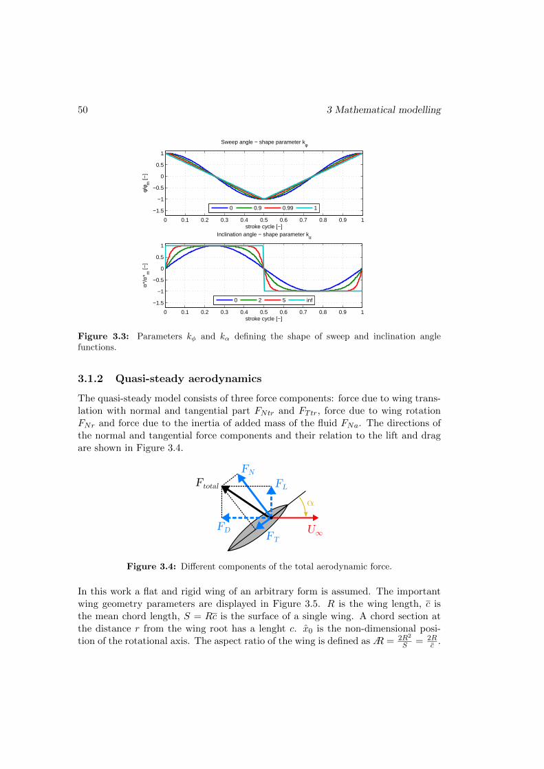
50 3 Mathematical modelling
0 0.1 0.2 0.3 0.4 0.5 0.6 0.7 0.8 0.9 1
−1.5
−1
−0.5
0
0.5
1
stroke cycle [−]
φ/φ m
[−]
Sweep angle − shape parameter kφ
0 0.9 0.99 1
0 0.1 0.2 0.3 0.4 0.5 0.6 0.7 0.8 0.9 1
−1.5
−1
−0.5
0
0.5
1
stroke cycle [−]
α*/α
* m [−
]
Inclination angle − shape parameter kα
0 2 5 inf
Figure 3.3: Parameters kφ and kα defining the shape of sweep and inclination anglefunctions.
3.1.2 Quasi-steady aerodynamics
The quasi-steady model consists of three force components: force due to wing trans-lation with normal and tangential part FNtr and FTtr, force due to wing rotationFNr and force due to the inertia of added mass of the fluid FNa. The directions ofthe normal and tangential force components and their relation to the lift and dragare shown in Figure 3.4.
Figure 3.4: Different components of the total aerodynamic force.
In this work a flat and rigid wing of an arbitrary form is assumed. The importantwing geometry parameters are displayed in Figure 3.5. R is the wing length, c isthe mean chord length, S = Rc is the surface of a single wing. A chord section atthe distance r from the wing root has a lenght c. x0 is the non-dimensional posi-tion of the rotational axis. The aspect ratio of the wing is defined asA = 2R2
S = 2Rc .

3.1 Flapping flight aerodynamics 51
dr
r2R
Centre of pressure
Wing centroid
c/2
c/2c/4
Axis of wing rotation
R
x0c
r
c(r)
Wing root
Figure 3.5: Wing geometry parameters
3.1.2.1 Force due to wing translation
The lift force due to translation of a 2D airfoil can be expressed according to anequation for fixed wing in steady flow as
F ′Ltr =1
2ρCL(α)cU2
∞, (3.2)
where ρ is the air density and CL is the lift coefficient.
If we consider hovering flapping flight and wing motion with 2 DOF the sectionspeed can be expressed as U∞(r) = rφ. For a wing with length R and mean chordc we introduce the non-dimensional section position and the non-dimensional chordlength as r = r
R and c = cc , respectively (Ellington, 1984a). The force of the whole
wing is given by an integral of the section force over the wing span
FLtr =
∫ R
0F ′Ltr(r)dr =
=1
2ρCL(α)φ2
∫ R
0c(r)r2dr =
=1
2ρCL(α)φ2R3c
∫ 1
0c(r)r2dr =
=1
2ρCL(α)Sr2
2R2φ2, (3.3)
where r22 =
∫ 10 c(r)r
2dr is the non-dimensional radius of the second moment of iner-tia. It defines the span-wise position of the centre of pressure where the forces with

52 3 Mathematical modelling
circulatory origin act. Its chord-wise position is assumed, similar to other studies,to be at one quarter of the chord from the leading edge (Figure 3.5), which is asimplification as Dickson et al. (2006) showed experimentally on a model wing thatthe location of the centre of pressure depends on the angle of attack.
The lift can also be formulated as a function of the centre of pressure speed UCP =r2
2R2φ2 as
FLtr =1
2ρCL(α)SU2
CP . (3.4)
Similar formulation can be written for the drag force
FDtr =1
2ρCD(α)SU2
CP . (3.5)
Since the remaining force components to be introduced in the next sections are allof a pressure origin and thus act normally to the wing chord it is convenient totransform the above lift and drag forces also into normal and tangential component(Deng et al., 2006)
FNtr =1
2ρCN (α)SU2
CP (3.6)
FTtr =1
2ρCT (α)SU2
CP . (3.7)
The normal and tangential force coefficients CN and CT were obtained by trans-formation of the empirical coefficients of Dickinson et al. (1999), which include theeffect of the delayed stall of the leading edge vortex, and have the following form
CN (α) = 3.4 sin(α) (3.8)
CT (α) =
0.4 cos2(2α) 0 ≤ |α| < π
40 π
4 ≤ |α| <3π4
−0.4 cos2(2α) 3π4 ≤ |α| < π.
(3.9)
3.1.2.2 Force due to wing rotation
Another force component that contributes to the total force generated by a flappingwing is the force due to wing rotation. It was derived from quasi-steady equationsused for flutter analysis (e.g. Fung, 1969). A translating wing that also starts torotate will develop additional circulation around itself to satisfy the Kutta condition(Ellington, 1984b). With the notation of Figure 3.5 this circulation can be expressedas
Γr = παc2
(3
4− x0
). (3.10)

3.1 Flapping flight aerodynamics 53
For a 2D airfoil the force is defined as
F ′Nr(r) = ρU∞Γr = πρc2
(3
4− x0
)U∞α. (3.11)
As a force of circulatory origin it acts at the centre of pressure and normally to thewing.
The total wing force is again obtained by integration over the wingspan while sub-stituting U∞(r) = rφ and introducing the non-dimensional position r and chord c
FNr =
∫ R
0F ′Nrdr =
= πρ
(3
4− x0
)αφR2c2
∫ 1
0c2(r)rdr. (3.12)
This can be rewritten further using the centre of pressure speed UCP as
FNr = ρπ
(3
4− x0
)αUCP
Rc2
r2
∫ 1
0c2(r)rdr. (3.13)
3.1.2.3 Force due to the inertia of added mass
The force due to the inertia of the added mass off the fluid can be formulated withthe help of equations originally introduced for flutter analysis. According to Fung(1969) this force consists of two components: a force due to the acceleration of anapparent mass and a centrifugal force.
The apparent mass acceleration force acts at the mid-chord (Figure 3.6). It is defined
as the apparent mass of a cylindrical section ρπ c2
4 times the normal acceleration
c/2
c/2
xr
C
rϕ
-rϕ.A
C'
A'
α
α*
aN
FNa
Figure 3.6: Wing section and parameters for calculation of the added mass force.

54 3 Mathematical modelling
aN of the mid-chord. Assuming hovering flight and wing motion with 2 DOF theacceleration of a wing section at a distance r from the wing root can be written as
aN (r) = xrα− rφ sinα, (3.14)
where xr is the distance of the axis of rotation A to the mid-chord C (Figure 3.6).Assuming further that this distance is equal to a quarter chord (xr = c
4) the forcebecomes
F ′Na(r) = ρπc2(r)
4aN (r) = ρπ
c2(r)
4
(c(r)
4α− rφ sinα
). (3.15)
The centrifugal force is a force of circulatory origin and is located at 3/4 of thechord from the leading edge. It is defined as the apparent mass times Uα, where Uis the component of relative wind speed in chord direction. For hovering flight with2 DOF the wing section force can be written as
F ′Nc(r) = ρπc2(r)
4
(−rφ cosα
)α. (3.16)
The total force is obtained by integration of the section forces over the wingspanwhile also introducing the non-dimensional position r and chord c
FNa =
∫ R
0
[F ′Na(r) + F ′Nc(r)
]dr =
= −1
4ρπR2c2
(φ sinα+ φα cosα
)∫ 1
0c2rdr +
1
16ρπRc3α
∫ 1
0c3dr. (3.17)
This formulation was presented by Maybury and Lehmann (2004), which is theformulation from Sane and Dickinson (2001) with additional corrections. Comparedto Maybury and Lehmann (2004) the terms including derivations of sweep angle φin our formulation differ in sign. This is due to an opposite definition of the positivedirection of φ.
3.1.2.4 Total force
Since the effects of the added mass inertia are relatively small compared to the othertwo components it will be neglected further in the text for simplicity. However, itseffects will be demonstrated at the end of this section. Thus, the total force of theflapping wing is a sum of forces due to translation and rotation
FN = FNtr + FNr =1
2ρCN (α)SU2
CP + ρπ
(3
4− x0
)αUCP
Rc2
r2
∫ 1
0c2(r)rdr
FT = FTtr =1
2ρCT (α)SU2
CP . (3.18)

3.1 Flapping flight aerodynamics 55
For a wing with given form the force varies only with the velocity of the centre ofpressure UCP and with the angle of attack α. The angle of attack is defined in Figure3.7 as the angle between the negative xW axis of the wing and the UCP velocity vec-tor. It can be either positive or negative, with values from the interval 〈−π, π〉. Thenormal component FN acts in zW direction (thus for hovering flight we get positivevalues in downstroke and negative in upstroke) and the tangential component FTacts in xW direction (in hover it is always positive or zero). The expressions for thecentre of pressure velocity and for the angle of attack for arbitrary flight conditionswill be derived in the following section.
xW
zW
UCP
FN
α
+α
FT
Downstroke Upstroke
α*
+α*
stroke planexSPySP CP
zB
xB
OB
+α +α*
α
α*
UCP
zW
xW
FT
FN
CP
stroke planexSPySP
Figure 3.7: Angle of attack α and orientation of normal, FN , and tangential, FT , forcecomponent in upstroke and downstroke (hovering flight). The figure displays right wingsection and considers β = 0 and δ = 0 for clarity.
3.1.3 Centre of pressure velocity and angle of attack
For hovering flight (body velocities and angular velocities are zero) and zero devi-ation from the stroke plane the aerodynamic angle of attack can be approximatedas α = sign (UCP )π/2 − α∗ (see Figure 3.7). Assuming further that the centre ofpressure (CP) lies on the span-wise rotation axis, its velocity is given by relationUCP = r2Rφ.
For a general case, when the body is in motion, the CP velocity is modified. Sincenot only the magnitude but also the direction of CP velocity changes, the aerody-namic angle of attack is also affected as can be seen in Figure 3.8 a). Situations,where angle of attack is negative or greater than 90 are sketched in 3.8 b) and 3.8c) respectively. Things get even more complicated when the wing deviates from thestroke plane and the rotation axis is not going through the CP.

56 3 Mathematical modelling
xW
zW
CP
UCPα
+α
velocity dueto flapping
velocity dueto body motion
stroke plane
zW xW
CP
+α
α
UCP
zW
xW
CP
+α
α
UCP
a) b) c)
Figure 3.8: Influence of body motion on the angle of attack; the figures represent theright wing cross-section and consider β = 0 and δ = 0 for clarity. a) Decomposition of thewing velocity into components due to flapping and due to body motion. b) Situation withnegative angle of attack. c) Situation with angle of attack greater than 90.
The motion of the wing with respect to the surrounding air can be decomposed intoa series of simultaneous motions. For their description we introduce three coordi-nate frames displayed in Figure 3.9 a) - global (inertial) frame G, body-fixed frameB and wing-fixed frame W. A left superscript with the frame letter will be used toindicate the coordinate system in which a vector or matrix is expressed. The originof the B frame is in the centre of gravity of the bird. In hover its axes are parallelto global frame axes with zB axis pointing towards the sky, xB axis in the backwardflight direction and yB axis in the direction of the right wing. The origin of thewing frame W is placed into the wing-root. The yW axis is aligned with the wingspanwise rotation axis, xW axis is parallel to the chord and pointing towards thetrailing edge of the wing and zW axis is normal to the wing surface, positive on thedorsal side of the wing.
OB
CP
xG
zG
yG
OG
U
rc
OWr
w
v
ω
r
ωw
OBxW
zW
yW
CPxB
zB
yB
xG
zG
yG
OG
OW
a) b)
Figure 3.9: Wing kinematics description. a) Introduced coordinate frames: global frameG, body-fixed frame B and wing-fixed frame W. b) Centre of pressure position and velocityas a result of simultaneous motions.
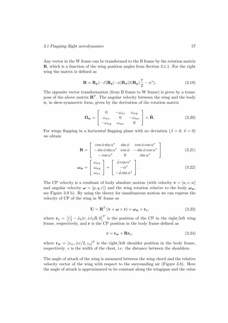
3.1 Flapping flight aerodynamics 57
Any vector in the W frame can be transformed to the B frame by the rotation matrixR, which is a function of the wing position angles from Section 3.1.1. For the rightwing the matrix is defined as
R = Ry(−β)Rz(−φ)Rx(δ)Ry(π
2− α∗). (3.19)
The opposite vector transformation (from B frame to W frame) is given by a trans-pose of the above matrix RT . The angular velocity between the wing and the bodyis, in skew-symmetric form, given by the derivation of the rotation matrix
Ωw =
0 −ωwz ωwyωwz 0 −ωwx−ωwy ωwx 0
= R. (3.20)
For wings flapping in a horizontal flapping plane with no deviation (β = 0, δ = 0)we obtain
R =
cosφ sinα∗ sinφ cosφ cosα∗
− sinφ sinα∗ cosφ − sinφ cosα∗
− cosα∗ 0 sinα∗
(3.21)
ωw =
ωwxωwyωwz
=
φ cosα∗
−α∗−φ sinα∗
. (3.22)
The CP velocity is a resultant of body absolute motion (with velocity v = [u, v, w]and angular velocity ω = [p, q, r]) and the wing rotation relative to the body ωw,see Figure 3.9 b). By using the theory for simultaneous motion we can express thevelocity of CP of the wing in W frame as
U = RT (v + ω × r) + ωw × rc, (3.23)
where rc =[(1
4 − x0)c,±r2R, 0]T
is the position of the CP in the right/left wingframe, respectively, and r is the CP position in the body frame defined as
r = rw + Rrc, (3.24)
where rw = [xw,±e/2, zw]T is the right/left shoulder position in the body frame,respectively. e is the width of the chest, i.e. the distance between the shoulders.
The angle of attack of the wing is measured between the wing chord and the relativevelocity vector of the wing with respect to the surrounding air (Figure 3.8). Herethe angle of attack is approximated to be constant along the wingspan and the value

58 3 Mathematical modelling
for the CP is used. The magnitude of the CP velocity vector in xWzW plane of thewing is
UCP =√U2x + U2
z . (3.25)
The effect of the spanwise component Uy on the aerodynamics is not considered.
According to Figure 3.8 the angle of attack can be computed as
α = atan2 (−Uz,−Ux) , (3.26)
where the atan2 is a four-quadrant inverse tangent function returning values between−π and π (MathWorks, 2014). The time derivative of the angle of attack can bederived from the above equation as
α =UzUx − UzUxU2x + U2
z
. (3.27)
The velocity derivations in the formula represent the change of CP velocity vectorin the wing frame and thus need to be carried out in that frame.
3.1.4 Comparison with CFD
To justify the use of quasi-steady aerodynamics and to show the importance of theforce component due to rotation, the instantaneous forces calculated by our modelare compared to CFD data. Lift, drag and side force curves from CFD study byZhang and Sun (2010a) are plotted in Figure 3.10 together with the curves result-ing from the quasi-steady model. To demonstrate the degree of importance of thequasi-steady model components, first only the force due to translation (3.6-3.7) isconsidered and the model is called ASL (tr). In model ASL (tr+rot) the force due torotation (3.13) is also included. Finally in model ASL (tr+rot+add) the last com-ponent due to the inertia of the added mass, similar to (3.17), is considered. Thedetails on the wing kinematics and morphology used are in (Karasek and Preumont,2012).
The forces are presented in the form of non-dimensional force coefficients defined asCL = FL/(0.5ρSU
2CP ) and similarly for CD and CY . UCP is the mean CP velocity
defined as UCP = 4φmf r2R. Lift FL is the force that is normal to the stroke plane.Drag FD lies inside the stroke plane and represents the force in an opposite directionto the wing instantaneous motion. Finally the side force FY represents the yB axiscomponent of the drag force. The curves start at cycle time t+ = 0, which is thepoint of reversal between upstroke and downstroke, the cycle is completed at t+ = 1.

3.1 Flapping flight aerodynamics 59
Lift Drag Y force
AS
L (
tr)
AS
L (
tr+
rot)
AS
L (
tr+
rot+
ad
d)
CF
D -
Zh
an
g&
Su
n
0 0.25 0.5 0.75 11
0
1
2
3
4
CL
[]
0 0.25 0.5 0.75 12
1
0
1
2
3
CD
[]
0 0.25 0.5 0.75 1
2
1
0
1
2
CY
[]
0 0.25 0.5 0.75 11
0
1
2
3
4
CL
[]
0 0.25 0.5 0.75 12
1
0
1
2
3
CD
[]
0 0.25 0.5 0.75 1
2
1
0
1
2
CY
[]
0 0.25 0.5 0.75 11
0
1
2
3
4
CL
[]
0 0.25 0.5 0.75 12
1
0
1
2
3
CD
[]
Flight Sideways Left Wing Flight Sideways Right Wing Reference Flight
0 0.25 0.5 0.75 1
2
1
0
1
2
CY
[]
0 0.25 0.5 0.75 11
0
1
2
3
4
CL
[]
t+
[ ]
0 0.25 0.5 0.75 12
1
0
1
2
3
t+
[ ]
CD
[]
0 0.25 0.5 0.75 1
2
1
0
1
2
CY
[]
t+
[ ]
Figure 3.10: Instantaneous forces over one flapping cycle predicted with quasi-steadymodel with increasing number of components and compared to CFD results of Zhang andSun (2010a).
60 3 Mathematical modelling
Apart from the wing forces in hovering conditions (dash-dotted line, lift and dragidentical for both wings), the left and right wing forces in sideways-flight with speedv = 0.15 UCP are also displayed. Good agreement of the force traces when the sys-tem is slightly deviated from its equilibrium is important for assessing the systemstability, which will be studied in the following section.
When we compare the CFD results (Figure 3.10, 4th row) to the force curves from thetranslational component model ASL (tr) (Figure 3.10, 1st row) it is clear, that sucha model is insufficient. On the contrary, the curves obtained by the ASL (tr+rot)model (Figure 3.10, 2nd row) show much better agreement with the CFD results.The rotational force component is responsible for the positive lift peak before andnegative lift peak after the stroke reversal. Similar peaks can be observed in dragand in the side force (both positive). Major differences occur after the reversal,where the forces predicted by the ASL (tr+rot) model drop, while positive peakscan be observed in the CFD force traces. The differences might be, at least partially,explained by the wake capture mechanism that is included only in the CFD model.
The addition of the added mass inertia component increases the magnitude of thecurves and further modifies the behaviour around the stroke reversal (Figure 3.10,3rd row). The accordance with the CFD results is slightly improved in some parts(lift peak and side force sign after the reversal) while in other parts the accordancegets worse (non-zero lift and drag force at the reversal). Thus, the overall improve-ment over the ASL (tr+rot) model force traces is insignificant, if any.
All the quasi-steady models over predict the CFD force magnitudes by about 20%.Considering that the used quasi-steady force coefficients were determined empiricallyfor a wing with different geometry and under different conditions, this difference isstill acceptable. Regardless the magnitudes, the shape of the force traces and thetrend of their changes, important for studying the stability and control of flappingflight, are captured with good accordance when the force due to rotation is used.
3.2 Body dynamics
The dynamics of the flying robot can be described, under rigid body assumption,by Newton-Euler motion equations. Similar to an aircraft we obtain 12 ordinarydifferential equations with 12 unknown coordinates - velocity (u, v, w), angular ve-locity (p, q, r), position (x, y, z) and orientation expressed by Roll-Pitch-Yaw angles(ϕ, ϑ, ψ) - see Figure 3.11. By omitting the equations for position and heading (yaw)

3.2 Body dynamics 61
angle ψ the system is reduced to 8 equations
u = − (wq − vr) +X/m+ g sinϑ
v = − (ur − wp) + Y/m− g cosϑ sinϕ
w = − (vp− uq) + Z/m− g cosϑ cosϕ
Ixxp = (Iyy − Izz) qr + Ixz (r + pq) + L
Iyy q = (Izz − Ixx) pr + Ixz(r2 − p2
)+M
Izz r = (Ixx − Iyy) pq + Ixz (p− qr) +N
ϕ = p+ q sinϕ tanϑ+ r cosϕ tanϑ
ϑ = q cosϕ− r sinϕ, (3.28)
where m is the body mass and Ixx, Iyy, Izz and Ixz are the non-zero moments andproduct of inertia in body frame (products Ixy and Iyz are both zero due to bodysymmetry). Aerodynamic forces and moments are represented by vectors (X,Y, Z)and (L,M,N) respectively.
xB
zB
yB
u, X
v, Y
w, Z
φp, L
ψr, N
ϑq, M
OB
Yaw
Roll
Pitch
Figure 3.11: Definition of body coordinates
There are two main types of aerodynamic forces to be considered: wing forces anddrag of body, legs and tail. According to Ristroph et al. (2013) the body drag forcebecomes important only in miligram-scale insects and legs and tail need to be con-sidered only in specific species. Xiong and Sun (2008) showed, that the body effectsbecome significant only for higher forward speeds. Thus, all drag-type forces areneglected and only the wing forces are considered further.

62 3 Mathematical modelling
The wing forces (3.18) are transformed into the body frame as follows
[X,Y, Z]T =∑i
[Xi, Yi, Zi]T =
∑i
Ri [FT i, 0, FNi]T (3.29)
[L,M,N ]T =∑i
rci × [Xi, Yi, Zi]T , (3.30)
where index i stands for the left and the right wing.
3.2.1 System linearisation
The mathematical model introduced in the previous sections is nonlinear and wasused in flight simulations. For stability studies and control design a linear model ispreferred.
The system dynamics (3.28) include aerodynamic forces and moments (3.29, 3.30)that are functions of wing motion parameters p = [f , βL, φmL, φ0L, αmL, α0L, ϕαL,δm1L, δm2L, βR, · · · , δm2R]T , system state x = [u, v, w, p, q, r, ϕ, ϑ]T and time t.Assuming the flapping frequency is much higher than the bandwidth of the system,the aerodynamic forces can be replaced by their cycle averaged values (mean valuesover one wingbeat), e.g.
X =
∫ 1f
0X(x,p, t)dt = X(x,p), (3.31)
that depend only on x and p. Small perturbation theory is used to rewrite the statesand wing motion parameters as
x = xe + δx, p = pe + δp, (3.32)
where subscript e signifies the equilibrium values and δ symbol stands for the per-turbation. The aerodynamic forces and moments are approximated by the linearterms of Taylor’s expansion. For the x-axis force we obtain
X(x,p) = Xe(xe,pe) +6∑i=1
∂X
∂xi(xe,pe)δxi +
n∑j=1
∂X
∂pj(xe,pe)δpj , (3.33)
where Xe is the cycle averaged force generated in equilibrium and n is the numberof wing kinematic parameters. The terms of the first summation are the derivativeswith respect to body velocities and angular velocities called the stability derivatives.If taken with an opposite sign they represent aerodynamic damping. The secondsummation terms are the derivatives with respect to changes in wing motion. They
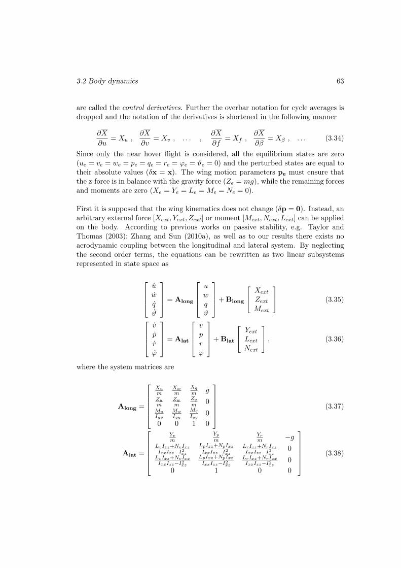
3.2 Body dynamics 63
are called the control derivatives. Further the overbar notation for cycle averages isdropped and the notation of the derivatives is shortened in the following manner
∂X
∂u= Xu ,
∂X
∂v= Xv , . . . ,
∂X
∂f= Xf ,
∂X
∂β= Xβ , . . . (3.34)
Since only the near hover flight is considered, all the equilibrium states are zero(ue = ve = we = pe = qe = re = ϕe = ϑe = 0) and the perturbed states are equal totheir absolute values (δx = x). The wing motion parameters pe must ensure thatthe z-force is in balance with the gravity force (Ze = mg), while the remaining forcesand moments are zero (Xe = Ye = Le = Me = Ne = 0).
First it is supposed that the wing kinematics does not change (δp = 0). Instead, anarbitrary external force [Xext, Yext, Zext] or moment [Mext, Next, Lext] can be appliedon the body. According to previous works on passive stability, e.g. Taylor andThomas (2003); Zhang and Sun (2010a), as well as to our results there exists noaerodynamic coupling between the longitudinal and lateral system. By neglectingthe second order terms, the equations can be rewritten as two linear subsystemsrepresented in state space as
uwq
ϑ
= Along
uwqϑ
+ Blong
Xext
ZextMext
(3.35)
vprϕ
= Alat
vprϕ
+ Blat
YextLextNext
, (3.36)
where the system matrices are
Along =
Xum
Xwm
Xqm g
Zum
Zwm
Zqm 0
MuIyy
MwIyy
Mq
Iyy0
0 0 1 0
(3.37)
Alat =
Yvm
Ypm
Yrm −g
LvIzz+NvIxzIxxIzz−I2xz
LpIzz+NpIxzIxxIzz−I2xz
LrIzz+NrIxzIxxIzz−I2xz
0LvIxz+NvIxxIxxIzz−I2xz
LpIxz+NpIxxIxxIzz−I2xz
LrIxz+NrIxxIxxIzz−I2xz
0
0 1 0 0
(3.38)

64 3 Mathematical modelling
and the control matrices are
Blong =
1m 0 0
0 1m 0
0 0 1Iyy
0 0 0
(3.39)
Blat =
1m 0 0
0 IzzIxxIzz−I2xz
IxzIxxIzz−I2xz
0 IxzIxxIzz−I2xz
IxxIxxIzz−I2xz
0 0 0
. (3.40)
In reality, the control forces and moments will be generated by the wings. From theapproximation in (3.33) a relation between the vector of cycle averaged forces andmoments and the modifications of wing kinematics parameters ∆p can be writtenas
[X,Y, Z, L,M,N ]T = J∆p, (3.41)
where J is the matrix of control derivatives defined as
J =
Xp1 Xp2 · · · Xpn
Yp1 Yp2 · · · Ypn...
.... . .
...Np1 Np2 · · · Npn
. (3.42)
The kinematic parameters modifications that should produce desired forces/momentsare estimated by a pseudoinverse of the previous relation
∆p = J+[X,Y, Z, L,M,N ]T . (3.43)
3.2.2 Stability and control derivatives
The stability and control derivatives are computed numerically. For example, thevalue of Xu can be obtained from the mean force X computed for small positive andfor small negative forward velocity ∆u and −∆u, respectively, while keeping otherstates x and wing motion parameters in their equilibrium values xe and pe.
Xu =∂X
∂u∼=X(xe + ∆u,pe)− X(xe −∆u,pe)
2∆u, (3.44)
where ∆u = [∆u, 0, 0, 0, 0, 0]. Other stability and control derivatives are obtainedin a similar manner.

3.3 Reduced model of a flapping wing MAV 65
3.3 Reduced model of a flapping wing MAV
In hovering flapping flight, many of the stability derivatives can be dropped. As-suming symmetric wing motion and wing shoulders placed in the zByB plane of thebody, derivatives Xw, Zu, Zq and Mw will be zero in the longitudinal system andYr, Lr, Nv and Np in the lateral system. This simplifies the system matrices Along
and Alat substantially as many of the cross-coupling terms disappear.
In natural fliers the forward flight is the preferred motion. Thus, even in hoveringtheir body posture stays inclined slightly forward with respect to the vertical axis.Due to the definition of the body axes (Figure 3.11) the product of inertia Ixz isnon-zero and is responsible for the coupling of roll and yaw. Most hovering MAVs,on the other hand, are designed so that hovering is the nominal operating point andso their body posture is vertical and Ixz = 0, which decouples yaw from the rest ofthe system.
Thus, the flapping MAV dynamics can be modelled by four subsystems:
• the pitch dynamics (u, q, ϑ)
uq
ϑ
=
Xu Xq g
Mu Mq 0
0 1 0
uqϑ
+
1 0
0 1
0 0
[ Xext
Mext
](3.45)
• the vertical dynamics (w)
w = Zww + Zext (3.46)
• the roll dynamics (v, p, ϕ)
vpϕ
=
Yv Yp −gLv Lp 0
0 1 0
vpϕ
+
1 0
0 1
0 0
[ YextLext
](3.47)
• the yaw dynamics (r)
r = Nrr + Next, (3.48)
where the following shortened notation was used: Xu = Xu/m, etc. for force deriva-tives, Mu = Mu/Iyy, etc. for moment derivatives, Xext = Xext/m, etc. for externalforces and Lext = Lext/Ixx for external moments.

66 3 Mathematical modelling
3.4 Stability predicted by various aerodynamic models
The objective of this section is to compare the pole locations of various models,including CFD, to justify the use of quasi-steady aerodynamics and cycle-averagingapproximations near hovering. This section is based on the results published in(Karasek and Preumont, 2012).
Similar to the model developed in the preceding sections, all the models consideredin the comparison employ the rigid body assumption: the periodic effects due to flap-ping are neglected and only the cycle averaged forces are applied on a rigid body,whose equations of motion are linearised, subsequently. The validity of the rigidbody assumption was confirmed by Zhang and Sun (2010b) who coupled Navier-Stokes equations with equations of motion and, for small amplitude disturbances,observed no major difference from the cycle-averaged linearised model even for ahawkmoth with relatively low flapping frequency (26.1 Hz).
Because the studied systems (3.35-3.36) are reachable and, assuming all the statesbeing accessible, also observable, the poles and respective modes of motion of theinsect can be computed as eigenvalues and eigenvectors of the linearised system ma-trices Along (3.37) and Alat (3.38). The stability derivatives that appear in thelinearised model are calculated based on the wing aerodynamics in all the models;the body drag is not considered as it was found to be negligible near hover (Sun andXiong, 2005).
It is difficult to measure the stability derivatives directly on flying animals as itwould require “deactivation” of all their control system to obtain correct data (Tay-lor and Thomas, 2003). Thus, most of the published data come from numericalstudies. The model animal that will be studied in this section was chosen to be adrone-fly, because CFD-based results are available both for longitudinal (Wu andSun, 2009) and lateral dynamics (Zhang and Sun, 2010a) for this insect. The im-portant morphological and wing kinematics parameters are in Table 3.1.
Models from Cheng and Deng (2011) and Orlowski and Girard (2011) based onquasi-steady aerodynamics are also included in the comparison. They consider onlythe force component due to translation, equivalent to (3.6-3.7), but provide analyticexpressions of the stability derivatives that can be evaluated for any animal or MAV.Similar to the comparison of force traces in Section 3.1.4 the quasi-steady modelfrom this chapter is represented three times: ASL (tr) includes only the force due totranslation (3.6-3.7), ASL (tr+rot) adds the force due to rotation (3.13) and finallyASL (tr+rot+add) adds also the component due to the inertia of the added mass,which is similar to (3.17).

3.4 Stability predicted by various aerodynamic models 67
f φm m Ixx Iyy Izz Ixz R A
(Hz) () (mg) (kg.m2) (kg.m2) (kg.m2) (kg.m2) (mm) (-)
164 53.55 87.76 6.58e-10 1.31e-9 8.35e-10 -5.50e-10 11.2 7.52
Table 3.1: Dronefly wing and morphological parameters.
3.4.1 Stability derivatives
The stability derivatives resulting from all the considered models are summarisedin Table 3.2 for longitudinal and in Table 3.3 for lateral system. As in the case ofthe reduced MAV model from the previous section, many of the derivatives are zeroor negligible (compared to derivatives of the same type, i.e. with the same units)no matter what aerodynamic model is used, namely Xw, Zu, Zq and Mw in thelongitudinal system and Yr, Lr, Nv and Np in the lateral system. Thus, the verticalmotion w is aerodynamically decoupled from the rest of the longitudinal system(u, q, ϑ) and the yaw rotation r is aerodynamically decoupled from the rest of thelateral system (v, p, ϕ). Nevertheless, there still exists coupling of roll p and yaw rthrough the inertia product Ixz. All the coordinates were defined in Figure 3.11.
ModelXu Xq Zw Mu Mq
(s-1) (ms-1) (s-1) (m-1s-1) (s-1)
Wu and Sun (2009) (CFD)* -2.22 0.0095 -2.03 -638 -1.65ASL (tr+rot+add) -3 -0.0641 -4.7 -691 -9.94
ASL (tr+rot) -3 -0.0539 -4.7 -607 -9.58ASL (tr) -3 -0.00549 -4.7 -369 -3.18
Cheng and Deng (2011) -2.67 0 -3.63 -328 -2.87Orlowski and Girard (2011) -2.74 0 -3.8 -243 -3.11
Table 3.2: Stability derivatives - longitudinal system. ∗Further non-zero derivatives werefound by the CFD study of Wu and Sun (2009): Xw = 0.179 s-1, Zu = −0.108 s-1, Zq =
0.0012 ms-1, Mw = 43.0 m-1s-1.
When comparing the stability derivatives from the quasi-steady models to the CFDresults the conclusions are ambiguous: for some derivatives we get the same signand similar magnitude for all the models (e.g. Xu, Yv, Nr) while for many othersthere exists no clear correspondence as the magnitudes and sometimes even the signsdiffer. On the other hand, not all the stability derivatives affect the stability (systempoles) in the similar manner. As has been shown in Sun et al. (2007) and Zhangand Sun (2010a) the most important derivatives with respect to stability are Xu,Zw, Mu, Mq (longitudinal system) and Lv, Lp, Nr (lateral system).

68 3 Mathematical modelling
ModelYv Yp Lv Lp Nr
(s-1) (ms-1) (m-1s-1) (s-1) (s-1)
Zhang and Sun (2010a)* (CFD) -1.57 0.0043 -575 -19.7 -25.8ASL (tr+rot+add) -1.26 -0.0606 -692 -21.4 -29.6
ASL (tr+rot) -1.26 -0.0609 -429 -20.8 -29.2ASL (tr) -1.26 0.00228 310 -37.6 -29.2
Cheng and Deng (2011) -1.11 0 272 -20.6 -21.5
Table 3.3: Stability derivatives - lateral system. ∗Further non-zero derivatives were foundby the CFD study of Zhang and Sun (2010a): Lr = 0.0493 s-1, Nv = −21.4 m-1s-1, Np =−1.54 s-1.
3.4.2 Longitudinal system poles
If it was difficult to make some conclusions from the control derivatives values, thepole maps make the situation much easier to understand. The longitudinal systempoles are given in Table 3.4. The pole map in Figure 3.12 shows that althoughthe pole locations vary among the different models, the general distribution remainsthe same: we always see a pair of complex conjugate poles with positive real part,resulting into an unstable oscillatory natural mode, and two negative real poles,representing fast and slow stable natural modes, called subsidence modes by Wuand Sun (2009).
It can be observed that even the simplest models, Cheng & Deng, Orlowski & Girardand ASL (tr), with only translational component give us poles which are reasonablyclose to the CFD study. If we add the components due to rotation and added massinertia, the oscillatory mode poles move towards the CFD poles, on the other handthe fast stable mode pole moves away from its CFD counterpart.
ModelLongitudinal system
λ1,2 (Mode 1) λ3 (Mode 2) λ4 (Mode 3)
Wu and Sun (2009) 7.88 ± 16i -19.6 -2.03ASL (tr+rot+add) 5.87 ± 15.5i -24.7 -4.7
ASL (tr+rot) 5.47 ± 14.9i -23.5 -4.7ASL (tr) 5.68 ± 13.2i -17.5 -4.7
Cheng and Deng (2011) 5.57 ± 12.7i -16.7 -3.63Orlowski and Girard (2011) 4.76 ± 11.5i -15.4 -3.8
Table 3.4: Poles of the longitudinal system

3.4 Stability predicted by various aerodynamic models 69
The eigenvectors (Table 3.6) further show that all the natural modes are estimatedreasonably well both in amplitude as well as in phase for all the models. The slowstable subsidence mode (Mode 3), representing the motion in vertical direction w,is decoupled from the rest. The remaining two modes are dominated by horizontalmotion u coupled with pitch rotation q. These two motions are in phase for Mode2 (fast subsidence), but almost in anti-phase (phase difference always greater than120) for Mode 1 (unstable oscillatory).
−25 −20 −15 −10 −5 0 5−20
−15
−10
−5
0
5
10
15
Re (λ)
Im (λ)
Wu (CFD)
ASL(tr+rot+add)
ASL(tr+rot)
ASL(tr)
Cheng
Orlowski*
Dronefly − longitudinal stability
Figure 3.12: Pole map - longitudinal system. All the models show similar dynamic be-haviour.
3.4.3 Lateral system poles
In the lateral direction the situation is different, see Table 3.5 and Figure 3.13. Thequasi steady based models with only translational force, Cheng & Deng and ASL(tr), predict one pair of complex conjugate poles with positive real part, resultinginto unstable oscillatory mode, and two negative real poles, representing fast andslow stable subsidence modes. On the contrary the models where rotational forceis included as well as the CFD model predict a positive real pole, representing aslow unstable divergence mode, a pair of complex conjugate poles with negative realparts (a stable oscillatory mode) and a negative real pole (fast subsidence mode).This shows the importance of the rotational force component on the stability results.

70 3 Mathematical modelling
ModelLateral system
λ5(5,6) (Mode 4) λ6,7(7) (Mode 5) λ8 (Mode 6)
Zhang and Sun (2010a) 12.9 -14.6 ± 9.32i -83.7ASL (tr+rot+add) 14.3 -15.1 ± 9.33i -98.8
ASL (tr+rot) 11.5 -13.5 ± 7.87i -97.2ASL (tr) 0.274 ± 8.64i -20.3 -130
Cheng and Deng (2011) 1.25 ± 10.1i -14.9 -82.5
Table 3.5: Poles of the lateral system
−140 −120 −100 −80 −60 −40 −20 0−15
−10
−5
0
5
10
Re (λ)
Im (λ)Dronefly − lateral stability
Zhang (CFD)
ASL(tr+rot+add)
ASL(tr+rot)
−140 −120 −100 −80 −60 −40 −20 0−15
−10
−5
0
5
10
Re (λ)
Im (λ)
ASL(tr)
Cheng
Figure 3.13: Pole map - lateral dynamics. Results divided into two figures according tothe pole location structure: CFD study Zhang and Sun (2010a) and quasi-steady modelsthat include rotational force (top) and quasi-steady models based only on translational force(bottom).

3.4
Stab
ilityp
redicted
by
various
aerod
yn
amic
mod
els71
Wu andSun (2009), ASL ASL ASL Cheng and Orlowski andZhang and (tr+rot+add) (tr+rot) (tr) Deng (2011) Girard (2011)
Sun (2010a)
Mode 1
u 0.522 (56.9) 0.531 (66.3) 0.556 (65.3) 0.619 (57.1) 0.647 (57.1) 0.715 (56.9)w 0.004 (-49.1) 0 (0) 0 (0) 0 (0) 0 (0) 0 (0)q 17.859 (-63.8) 16.578 (-69.3) 15.910 (-69.9) 14.369 (-66.7) 13.901 (-66.4) 12.444 (-67.5)ϑ 1 (0) 1 (0) 1 (0) 1 (0) 1 (0) 1 (0)
Mode 2
u 0.553 (180) 0.526 (180) 0.540 (180) 0.682 (180) 0.701 (180) 0.777 (180)w 0.002 (180) 0 (0) 0 (0) 0 (0) 0 (0) 0 (0)q 19.626 (180) 24.667 (180) 23.513 (180) 17.527 (180) 16.668 (180) 15.373 (180)ϑ 1 (0) 1 (0) 1 (0) 1 (0) 1 (0) 1 (0)
Mode 3
u 3.965 (180) 0 (0) 0 (0) 0 (0) 0 (0) 0 (0)w 58.792 (180) 1 (0) 1 (0) 1 (0) 1 (0) 1 (0)q 2.034 (180) 0 (0) 0 (0) 0 (0) 0 (0) 0 (0)ϑ 1 (0) 0 (0) 0 (0) 0 (0) 0 (0) 0 (0)
Mode 4
v 0.675 (180) 0.686 (180) 0.821 (180) 1.118 (100) 0.945 (103) -p 12.888 (0) 14.310 (0) 11.534 (0) 8.644 (88.2) 10.186 (82.9) -r 2.972 (180) 3.076 (180) 2.152 (180) 1.603 (20) 2.743 (38) -ϕ 1 (0) 1 (0) 1 (0) 1 (0) 1 (0) -
Mode 5
v 0.616 (35.3) 0.533 (37.6) 0.619 (35.8) 0.519 (0) 0.710 (0) -p 17.325 (147) 17.775 (148) 15.623 (150) 20.263 (180) 14.926 (180) -r 11.892 (74.6) 12.120 (83.8) 9.158 (92.9) 30.264 (180) 22.222 (180) -ϕ 1 (0) 1 (0) 1 (0) 1 (0) 1 (0) -
Mode 6
v 0.124 (0) 0.039 (0) 0.041 (0) 0.078 (0) 0.121 (0) -p 83.682 (180) 98.839 (180) 97.176 (180) 130.466 (180) 82.518 (180) -r 77.503 (0) 92.924 (0) 91.553 (0) 110.773 (0) 73.580 (0) -ϕ 1 (0) 1 (0) 1 (0) 1 (0) 1 (0) -
Table 3.6: Eigenvectors of the longitudinal (Modes 1-3) and lateral system (modes 4-6) showing the amplitude and phase (inparenthesis). Longitudinal system values are normalized by pitch ϑ, lateral by roll ϕ.

72 3 Mathematical modelling
The addition of the third component due to added mass inertia further moves thecomplex pair of poles towards the CFD results.
From the eigenvectors in Table 3.6 we see that the dominant motion in Mode 4 isthe sideways motion v. For the first three models it is in anti-phase with roll pbut in phase with yaw r. In the remaining models, ASL(tr) and Cheng & Deng,the sideways motion and roll are nearly in phase, the phase difference from yaw issmaller than 90. Mode 5 is a combination of the three motions v, p, r. In thefirst three models the sideways motion and roll are out of phase by about 110 andthe yaw phase lies approximately in between. In the remaining models the sidewaysmotion is in anti-phase with roll and yaw rotation. Mode 6, similar in all the models,represents the out of phase coupling of roll and yaw.
3.4.4 Effect of derivatives Xq and Yp
In Section 3.4.1 it was shown that various models predict very similar dynamic be-haviour, even though the sign of stability derivatives Xq and Yp varies among themodels. This suggests that these derivatives have very small effect on the dynamics.The comparison of pole positions for the full system and for the system with Xq = 0and Yp = 0 is in Table 3.7. The differences are indeed very small and, therefore, thederivatives Xq and Yp can be neglected in the preliminary analyses.
ModelLongitudinal system Lateral system
λ1,2 λ3 λ5(5,6) λ6,7(7) λ8
Wu&Sun (2009) / 7.88 ± 16i -19.6 12.9 -14.6 ± 9.32i -83.7Zhang&Sun (2010a) 7.94 ± 15.9i -19.7 12.9 -14.6 ± 9.28i -83.7
ASL (tr+rot+add)5.87 ± 15.5i -24.7 14.3 -15.1 ± 9.33i -98.85.39 ± 16i -23.7 13.8 -15.3 ± 9.9i -98
ASL (tr+rot)5.47 ± 14.9i -23.5 11.5 -13.5 ± 7.87i -97.25.1 ± 15.3i -22.8 11.2 -13.6 ± 8.32i -96.7
ASL (tr)5.68 ± 13.2i -17.5 0.274 ± 8.64i -20.3 -1305.65 ± 13.2i -17.5 0.266 ± 8.64i -20.3 -130
Table 3.7: Effect of derivatives Xq and Yp on the system poles: complete system (black),
Xq and Yv neglected (red). Only the poles and models that were affected are displayed.
3.4.5 Effect of inertia product Ixz
While in longitudinal system the vertical dynamics is decoupled from the pitch, acoupling between yaw and roll exists in the lateral system due to the inertia product

3.4 Stability predicted by various aerodynamic models 73
Ixz. Assuming the dronefly body posture in hovering is vertical (as in most hoveringMAVs), the inertia product Ixz becomes zero and the coupling disappears. Theresulting pole locations are shown in Figure 3.14 and listed in Table 3.8.
We can observe some differences compared to the nominal body posture (inclined by48 from the vertical axis), nevertheless the pole distribution remains the same. Thebiggest difference is in the fastest stable real pole, which after decoupling representsthe yaw dynamics. On the other hand, the remaining poles (now representing theroll and lateral dynamics) represent still a good approximation of the original sys-tem. Hence, the roll and lateral dynamics can be in the first approximation treatedindependently of yaw, which greatly simplifies the problem of stability and controldesign, as will be shown in the next chapter.
− 40 −120 −100 −80 −60 −40 −20 0−15
−10
−5
0
5
10
Re ( )
Im ( )
140 120 100 80 60 40 20 015
10
5
0
5
10
Re ( )
Im ( )Dronefly lateral stability
Zhang (CFD)
ASL(tr+rot+add)
ASL(tr+rot)
ASL(tr)
Cheng
Ixz≠0 Ixz=0
Figure 3.14: Effect of inertia product Ixz on the lateral poles: nominal body posture(Ixz 6= 0) in blue, vertical posture (Ixz = 0) in red. Results split into two parts accordingto the pole location structure: CFD study Zhang and Sun (2010a) and quasi-steady modelsthat include rotational force (top), quasi-steady models based only on translational force(bottom).

74 References
ModelLateral system
λ5(5,6) λ6,7(7) λ8
Zhang and Sun (2010a)12.9 -14.6 ± 9.32i -83.710.9 -11.2 ± 11.6i -113
ASL (tr+rot+add)14.3 -15.1 ± 9.33i -98.811.7 -11.9 ± 12.3i -130
ASL (tr+rot)11.5 -13.5 ± 7.87i -97.29.65 -10.7 ± 10.3i -128
ASL (tr)0.274 ± 8.64i -20.3 -130
1 ± 8.23i -22.3 -128
Cheng and Deng (2011)1.25 ± 10.1i -14.9 -82.52.26 ± 8.88i -16 -94.6
Table 3.8: Effect of inertia product Ixz on the system poles: original body posture (Ixz 6= 0,black), vertical body posture (Ixz = 0, red).
3.4.6 Conclusion
It was shown that the stability of the flapping flight in hover can be successfullyestimated while using a quasi-steady based model that includes components dueto rotation and translation. Despite the simplifications used (the effective angle ofattack and relative wing velocity were considered constant along the wingspan, thecentre of pressure was placed on the wing spanwise rotation axis) the results arecomparable to the ones obtained by CFD modelling, while the necessary compu-tation power is significantly reduced. Therefore such a quasi-steady model can beadvantageously used in flapping-wing MAV parameter and control design. However,the model, assuming rigid wings, will still remain a rather gross approximation asthe wings of many natural fliers as well as of most MAVs are flexible.
The linearised model was further reduced by neglecting the inertia product Ixz andderivatives Xq and Yp, whose effects on the pole locations were shown to be verysmall. Thus, the dynamics of hovering flapping flight can be described by only 8stability derivatives and splits into 4 subsystems (pitch, roll, yaw and vertical dy-namics) that can be treated separately in the control design.
3.5 References
G. J. Berman and Z. J. Wang. Energy-minimizing kinematics in hover-ing insect flight. Journal of Fluid Mechanics, 582:153–168, Jun. 2007.

References 75
doi:10.1017/S0022112007006209.
B. Cheng and X. Deng. Translational and rotational damping of flapping flight andits dynamics and stability at hovering. IEEE Transactions on Robotics, 27(5):849–864, Oct. 2011. doi:10.1109/TRO.2011.2156170.
X. Deng, L. Schenato, W. C. Wu, and S. S. Sastry. Flapping flight for biomimeticrobotic insects: part I-system modeling. IEEE Transactions on Robotics, 22(4):776–788, Aug. 2006. doi:10.1109/TRO.2006.875480.
M. H. Dickinson, F.-O. Lehmann, and S. P. Sane. Wing rotation and theaerodynamic basis of insect flight. Science, 284(5422):1954–1960, Jun. 1999.doi:10.1126/science.284.5422.1954.
W. B. Dickson, A. D. Straw, C. Poelma, and M. H. Dickinson. An integrative modelof insect flight control. 44th AIAA Aerospace Sciences Meeting and Exhibit; Reno,NV; USA; 9-12 Jan, pages 1–19, 2006.
C. P. Ellington. The aerodynamics of hovering insect flight. II. Morphological pa-rameters. Philosophical Transactions of the Royal Society of London. Series B,Biological Sciences, 305(1122):17–40, Feb. 1984a. doi:10.1098/rstb.1984.0050.
C. P. Ellington. The aerodynamics of hovering insect flight. IV. aerodynamic mech-anisms. Philosophical Transactions of the Royal Society of London. Series B,Biological Sciences, 305(1122):79–113, Feb. 1984b.
Y. C. Fung. An introduction to the theory of aeroelasticity. Dover, New York, 1969.
M. Karasek and A. Preumont. Flapping flight stability in hover: A comparison ofvarious aerodynamic models. International Journal of Micro Air Vehicles, 4(3):203–226, 2012. doi:10.1260/1756-8293.4.3.203.
MathWorks. Matlab documentation: atan2 function. http://www.mathworks.com/help/matlab/ref/atan2.html, 2014. Accessed: 18/08/2014.
W. J. Maybury and F.-O. Lehmann. The fluid dynamics of flight control by kine-matic phase lag variation between two robotic insect wings. Journal of Experi-mental Biology, 207:4707–4726, 2004. doi:10.1242/jeb.01319.
C. T. Orlowski and A. R. Girard. Stability derivatives for a flapping wing MAV ina hover condition using local averaging. In 2011 American Control Conf., pages1604–1609, San Francisco, California, Jun. - Jul. 2011.
G. D. Padfield. Helicopter Flight Dynamics: The Theory and Application of FlyingQualities and Simulation Modeling. Blackwell Science Ltd., 2nd edition, 2007.

76 References
L. Ristroph, G. Ristroph, S. Morozova, A. J. Bergou, S. Chang, J. Gucken-heimer, Z. J. Wang, and I. Cohen. Active and passive stabilization of bodypitch in insect flight. Journal of The Royal Society Interface, 10(85):1–13, 2013.doi:10.1098/rsif.2013.0237.
S. P. Sane and M. H. Dickinson. The control of flight force by a flapping wing: liftand drag production. Journal of Experimental Biology, 204:2607–2626, 2001.
S. P. Sane and M. H. Dickinson. The aerodynamic effects of wing rotation and arevised quasi-steady model of flapping flight. Journal of Experimental Biology,205:1087–1096, 2002.
L. I. Sedov. Two-dimensional problems in hydromechanics and aerodynamics. In-terscience publishers, New York, 1965.
W. Shyy, H. Aono, C.-K. Kang, and H. Liu. An Introduction to Flapping WingAerodynamics. Cambridge University Press, 2013.
M. Sun and Y. Xiong. Dynamic flight stability of a hovering bumblebee. Journal ofExperimental Biology, 208:447–459, 2005.
M. Sun, J. Wang, and Y. Xiong. Dynamic flight stability of hovering insects. ActaMech. Sinica, 23(3):231–246, Jun. 2007. doi:10.1007/s10409-007-0068-3.
G. K. Taylor and A. L. R. Thomas. Dynamic flight stability in the desert locustschistocerca gregaria. Journal of Experimental Biology, 206(16):2803–2829, Aug.2003. doi:10.1242/jeb.00501.
J. Wu and M. Sun. Control for going from hovering to small speed flight of a modelinsect. Acta Mech. Sinica, 25(3):295–302, Jun. 2009. doi:10.1007/s10409-009-0241-y.
Y. Xiong and M. Sun. Dynamic flight stability of a bumblebee in forward flight.Acta Mech. Sinica, 24(1):25–36, Feb. 2008. doi:DOI 10.1007/s10409-007-0121-2.
Y. Zhang and M. Sun. Dynamic flight stability of a hovering model insect: lateralmotion. Acta Mech. Sinica, 26(2):175–190, May. 2010a. doi:10.1007/s10409-009-0303-1.
Y. Zhang and M. Sun. Dynamic flight stability of a hovering model insect: theoryversus simulation using equations of motion coupled with navier-stokes equation.Acta Mech. Sinica, 26(4):509–520, 2010b. doi:10.1007/s10409-010-0360-5.

Chapter 4
Stability of near-hover flappingflight
This chapter studies the stability of the developed hummingbird-like MAV aroundhovering. The linearised model of near-hover flapping flight from the previous chap-ter is employed. The choice of wing position for an easily controllable MAV isdiscussed and a simplified solution of the pitch and roll stability problem is pro-posed.
4.1 Hummingbird robot parameters
Since the existing models predict that the hovering flapping flight of natural fliers isunstable, it is very unlikely that a passively stable MAV design would exist (with-out additional stabilizing surfaces like sails). However, the mathematical model canhelp us identify a design that would be easily controllable. In this section a 20 ghummingbird-like MAV with parameters according to Table 4.1 will be studied. Thewing parameters were selected according to the robot prototype that will be pre-sented in Chapter 6, the mass properties are an estimate based on a CAD model.Vertical body orientation is assumed while hovering so the inertia product Ixz isequal to zero.
m Ixx Iyy Izz e R A r2 x0
∫ 10 c
2rdr*
(g) (kg.m2) (kg.m2) (kg.m2) (mm) (mm) (-) (-) (-) (-)
20 1e-5 1e-5 1e-3 31.6 90 9.33 0.531 0.25 0.418
Table 4.1: Hummingbird robot parameters, according to definitions in Chapter 3. *Wingshape characteristic in equation (3.13).
77

78 4 Stability of near-hover flapping flight
OB
xB
zB
yB
xBzw
xw
e
Figure 4.1: The position of the wing shoulders with respect to the COG.
Based on experiments that will be presented in Section 6.2 the wing operating con-ditions were estimated to a flapping amplitude φm = 80 and frequency f = 26 Hz.The value of the angle of attack in mid-stroke that provides an equilibrium betweenthe weight and the average lift force, αm = 33, was found by iterations. The lastbut very important design parameter is the position of the wings with respect to thecentre of gravity (Figure 4.1). Our intuition tells us that the wings should be higherthan the centre of gravity, which is also what can be observed in nature. To see itseffect the vertical wing position zw was kept as a free parameter. The longitudinalposition of the wings was set to xw = 0.
4.2 Pitch dynamics
The pitch dynamics is represented by the state space model uq
ϑ
=
Xu Xq g
Mu Mq 0
0 1 0
uqϑ
+
1 0
0 1
0 0
[ Xext
Mext
]. (4.1)
The positive directions of the coordinates are displayed in Figure 4.2.
4.2.1 Pitch stability derivatives
The stability of the pitch dynamics is determined by the stability derivatives Xu,Xq, Mu and Mq. Their values can be evaluated numerically by the aerodynamic
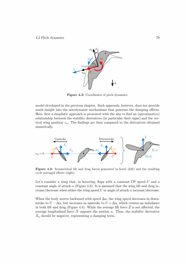
4.2 Pitch dynamics 79
xB
zB
OB
M
X
u
ϑ
q
g
Figure 4.2: Coordinates of pitch dynamics.
model developed in the previous chapter. Such approach, however, does not providemuch insight into the aerodynamic mechanisms that generate the damping effects.Here, first a simplistic approach is presented with the aim to find an (aproximative)relationship between the stability derivatives (in particular their signs) and the ver-tical wing position zw. The findings are then compared to the derivatives obtainednumerically.
zW = 0Z
M=0
X=0
Upstrokeα FD
FL
U
DownstrokeFD
FL αU
Figure 4.3: Symmetrical lift and drag forces generated in hover (left) and the resultingcycle averaged efforts (right).
Let’s consider a wing that, in hovering, flaps with a constant CP speed U and aconstant angle of attack α (Figure 4.3). It is assumed that the wing lift and drag in-crease/decrease when either the wing speed U or angle of attack α increase/decrease.
When the body moves backward with speed ∆u, the wing speed decreases in down-stroke to U −∆u, but increases in upstroke to U + ∆u, which creates an imbalancein both lift and drag (Figure 4.4). While the average lift force Z is not affected, theaverage longitudinal force X opposes the motion u. Thus, the stability derivativeXu should be negative, representing a damping term.

80 4 Stability of near-hover flapping flight
zW = 0Z
M=0
X<0
ΔuΔu
Upstrokeα ↑FD
↑FL↑U
Downstroke↓FD
↓FL α↓U
Figure 4.4: Effects of a disturbance in longitudinal direction ∆u when the wing shouldersare placed at the COG (zw = 0). A wing speed difference between upstroke and downstrokeinduces a cycle-averaged damping force X that opposes the disturbance.
zW<0
Upstroke Downstrokeα ↓FD
↓FL↑FD
↑FL αzW>0
Z
M<0
X<0
Z
M>0
Δu Δu
α ↓FD
↓FL↑FD
↑FL α X<0
Δu
Δu
↑U
↑U
↓U
↓U
Figure 4.5: Effects of a disturbance in longitudinal direction ∆u for a general wing shoulderposition (zw 6= 0). The cycle-averaged drag force acts at a lever zw and induces a pitchmoment M , whose sign is opposite to the sign of zw.
For a general wing shoulder position (zW 6= 0) a pitch moment M = Xzw arises dueto the lever arm from the wing shoulder to the COG (Figure 4.5). Therefore, Mu
should be positive below the COG and negative above the COG.
Rotating the body around the pitch axis with an angular rate ∆q affects both thewing speed and the angle of attack. Considering first the wing shoulders placed atthe COG (zW = 0), the principal effect is on the angle of attack α (Figure 4.6). Theangle increases for wing positions behind the body but decreases in front of the bodybecause of a vertical velocity component due to the body rotation. The resultingdifference in lift and drag averages out over one wingbeat, but the lift imbalance

4.2 Pitch dynamics 81
↓αUpstrokeΔq
zW = 0Downstroke
Δq
zW = 0
↑α ↑FD
↑FL ↓FD
↓FL
↓α↑α↑FD
↑FL ↓FD
↓FL
Z
M<0
Δq
X=0
Back Front
Figure 4.6: Effects of a pitch disturbance ∆q when the wing shoulders are placed at theCOG (zw = 0). The angle of attack increases behind the body, but decreases in front of thebody, which causes an uneven distribution of the lift force and results into a cycle-averagedpitch moment M that opposes the disturbance.
α ↓FD
↓FL ↑FD
↑FL αzW<0
Upstroke
Δq
Downstrokeα ↓FD
↓FL
Δq
↑FD
↑FL αzW>0
Z
M<0
Δq
X<0
Z
M<0
Δq
X>0
↑U
↑U↓U
↓U
Figure 4.7: Effects of a pitch disturbance ∆q for a general wing shoulder position (zw 6=0). On top of the angle of attack changes the speed increases/decreases in upstroke anddecreases/increases in downstroke when the wings shoulders are placed above/below theCOG, respectively. This induces a non-zero cycle averaged force X, whose sign is oppositeto the sign of zw, and decreases further the negative stabilizing pitch moment M for bothpositive and negative zW .

82 4 Stability of near-hover flapping flight
gives rise to a pitch moment M opposing the rotation ∆q. Thus, the derivative Mq
should be negative.
If the wing shoulders are placed above or below the COG, the wing speed is alsomodified in the central wing position (Figure 4.7). The speed increases in upstrokeand decreases in downstroke for zw > 0; the opposite is true for zw < 0. This cre-ates a drag asymmetry between upstroke and downstroke, which translates into thecycle averaged longitudinal force X. Therefore, the derivative Xq should be positivefor zw < 0 and negative for zw > 0. Further, the pitch moment gets modified toM = M0 +Xzw, where the first term represents the pitch damping moment for wingshoulders at COG (zw = 0). The second term is always smaller or equal to zero dueto opposite signs of X and zw. Thus, the derivative Mq should stay negative for anywing shoulder position.
−1.5
−1
−0.5
0
−0.1
0
0.1
−100
0
100
−30 −20 −10 0 10 20 30−10
−5
0
ASL(tr+rot) ASL(tr)
Xu [s-1
]
Xq [m
.s-1]
M
q [s-1
]
Mu [m
-1s-1
]
zw [mm]
Figure 4.8: Stability derivatives of pitch dynamics for varying wing position zW .
The stability derivatives given by the model presented in the previous chapter forrobot parameters given in Section 4.1 are plotted in Figure 4.8. Two quasi-steadymodels were used, a simpler model including only the force due to translation, ASL(tr), and a more complex model that includes also the force due to rotation, ASL

4.2 Pitch dynamics 83
(tr+rot). It has been shown in Section 3.4 that the latter gives comparable stabilityderivatives to a CFD model.
The simpler model ASL (tr) plotted in red dashed lines in Figure 4.8 is in completeagreement with the findings about the derivative signs based on Figures 4.4-4.7 madeearlier. The derivative Xu representing the damping of the forward translation isalways negative and independent on the wing position. The derivative Mq, the pitchrotation damping, remains always negative, varying with square of wing position z2
w
with a maximum at zw = 0. The cross-coupling derivatives Mu and Xq are zero forzw = 0 and vary linearly, with a negative slope, with the wing position zw.
The addition of the force due to rotation in ASL (tr+rot) has no effect on thederivative Xu (blue solid lines in Figure 4.8). We can observe some differencesamong the other three derivatives, but the general behaviour remains similar. Thepitch damping Mq remains approximately quadratic function of z2
w. Its maximumvalue, now at zw ≈ −18 mm, slightly increases, but stays negative. The derivativesXq and Mu are slightly offset from the simpler model, but keep the same slope. Xq
stays always negative in the studied range, while Mu crosses zero at around -4 mm.
4.2.2 System poles
Assuming a reachable and observable system with a system matrix A, the systempoles are defined as roots of the characteristic equation |λI − A| = 0. For pitchdynamics, we obtain a cubic equation
λ3 −(Xu + Mq
)λ2 +
(XuMq − MuXq
)λ− Mug = 0 (4.2)
with three roots. Figure 4.9 shows position of the poles (root locus) for wing po-sition zw ranging from -30 mm to 30 mm, calculated from the stability derivativesshown in Figure 4.8. In both models, ASL (tr) in red-dashed lines and ASL (tr+rot)in blue lines, we can observe 3 different pole configurations. For positive values ofzw (wings placed above the centre of gravity), we have a pair of complex unstablepoles and one real stable pole. For negative zw, there is one stable real pole and anunstable pair of complex poles. Finally, there is a narrow transient region aroundthe COG (zw ≈ 0) for ASL (tr) and below the COG (zw ≈ −4mm) for ASL (tr+rot)where 3 real poles exist.
It can be demonstrated that the pole configuration is determined by the derivativeMu. By neglecting the derivative Xq (whose effect on the dynamics has been shownto be very small, see Section 3.4.4) the characteristic equation becomes
λ3 −(Xu + Mq
)λ2 + XuMqλ− Mug = 0, (4.3)

84 4 Stability of near-hover flapping flight
−15 −10 −5 0 5 10−10
−5
0
5
10
−15 −10 −5 0 5 10−30
0
30
ASL (tr+rot)
ASL (tr)
Im (
λ)
z w [m
m]
Figure 4.9: Influence of wing position zw on the pitch dynamics: pole positions in complexplane (top) and real part of the poles against the wing position (bottom).
which can be rewritten as
λ(λ− Xu
)(λ− Mq
)− Mug = 0 (4.4)
or
1 + Mu−g
λ(λ− Xu
)(λ− Mq
) = 0. (4.5)
The equation has the same form as a characteristic equation of system H(s) =−g/(λ(λ− Xu)(λ−Mq)) in closed loop with a feedback gain Mu. Thus, a root locusmethod can be used to study the effect of the derivative Mu on the pitch dynamicspoles.
The system H(s) has three poles, one at the origin and two on the real axis givenby the derivatives Xu and Mq, respectively. Since H(s) has no zeros and a negativenumerator, the root locus will follow asymptotes at ±60 and 180 for Mu → −∞and asymptotes at 0 and ±120 for Mu → ∞. The start point of the asymptotes

4.2 Pitch dynamics 85
Re (λ)
Im (
λ)
0
0
Mq X
u
Mu → +∞
0
Mu → −∞
60°
120°
Mq + X
u
3
^ ^
Figure 4.10: Root locus showing the effect of derivative Mu on the system dynamics.
lies at (Xu + Mq)/3. The resulting root locus is shown in Figure 4.10 and looksvery similar to the locus for varying wing position zw (Figure 4.9): negative Mu
results into a pair of unstable complex poles and a stable real pole, while positiveMu results into an unstable real pole and a pair of stable complex poles.
Provided that both Xu and Mq are negative, a small region of stability exists forsmall negative values of Mu. This region, with one fast real pole and a pair of slowlightly damped complex poles, can only be enlarged by increasing the damping offorward translation or pitch rotation. This can be done either passively by addingsome damping surfaces (tail, sails) or actively by feedback control.
4.2.3 Active stabilization
Flying animals are equipped with sensory systems that provide feedback for activestabilization of their flight. As it has been mentioned already in Section 2.3.3, fliesuse two types of sensors to sense angular velocities: the compound eyes and the hal-teres. Compared to compound eyes, which are most sensitive to rates of the orderof 100/s, the halteres can sense rates up to 1000/s (Taylor and Krapp, 2008) andtheir latency is about four times shorter (Ristroph et al., 2013). Sherman and Dick-inson (2004) showed that the wing response simply follows a weighted sum of the twosensory signals. Thus, the aim of this section is to show under which conditions canthe pitch dynamics be stabilized using a simple angular rate feedback with a gain kq.

86 4 Stability of near-hover flapping flight
Such control will introduce a stabilizing moment M = −kqq. By plugging themoment into the state space model we get u
q
ϑ
=
Xu Xq g
Mu Mq − kq 0
0 1 0
uqϑ
+
1 0
0 1
0 0
[ Xext
Mext
], (4.6)
which yields the characteristic equation
λ3 +(kq − Xu − Mq
)λ2 +
[Xu
(Mq − kq
)− MuXq
]λ− Mug = 0. (4.7)
The necessary (but not sufficient) condition for stability requires that all coefficientsof the characteristic equation are positive. This already shows that the pitch ratefeedback can stabilize the system only if the derivative Mu is negative. By neglectingagain the derivative Xq and rewriting the characteristic equation into the root locusform with parameter Mu we obtain
1 + Mu−g
λ(λ− Xu
)(λ+ kq − Mq
) = 0. (4.8)
We can observe, that the feedback gain moves the pole related to the pitch ratedamping towards minus infinity (see Figure 4.11). This results into a shift of the
Re (λ)
Im (
λ)
0
0
Mq Xu
Mu → +∞
0
Mu → −∞
Mq − kq + Xu
3
^ ^
kq
CL
CL
OLOL
Figure 4.11: The effect of derivative Mu on the pitch dynamics in open loop (OL) and inclosed loop (CL) with pitch rate feedback kq.

4.2 Pitch dynamics 87
asymptotes origin to the left and causes an “opening” of the root locus for negativevalues of Mu. Thus, the system becomes stable for a much larger interval of thestability derivative Mu.
The minimal necessary gain for stability for a given Mu can be expressed by using theRouth-Hurwitz stability criterion (e.g. Franklin et al., 2002, p. 158). The criterionyields three conditions(
kq − Xu − Mq
) [Xu
(Mq − kq
)− MuXq
]+ Mug > 0 (4.9)
kq − Xu − Mq > 0 (4.10)
−Mug > 0. (4.11)
The third condition confirms that Mu must be negative. The second condition isusually fulfilled as both derivatives Xu and Mq are typically negative (see Table 4.2).Thus, the minimal gain can be expressed from the first condition. Since the gainshould be positive we obtain
kq,min =MuXq − 2XuMq − X2
u +
√(X2u + MuXq
)2+ 4XuMug
−2Xu
. (4.12)
For a typical hovering animal the minimal necessary gain is much higher than theremaining terms in the brackets on the left side of relation (4.9), namely kq,min (−Xu − Mq
)and kq,min
(−Mq +
MuXq
Xu
). By neglecting these terms, and keep-
ing in mind that Xu < 0, we obtain much simpler condition
kq >
√Mu
Xu
g, (4.13)
which can serve as a good first estimate of minimal necessary gain. Moreover, if
Mq <MuXq
Xu, all the terms neglected on the left side of the relation (4.9) are posi-
tive. In that case the relation (4.13) becomes a sufficient condition for stability.
Table 4.3 shows the poles computed for several animals using stability derivativesfrom Table 4.2. It also compares the values of the minimal feedback gain k cal-culated with the exact formula (4.12) and the values estimated by relation (4.13).We can see that in most cases the approximative formula is very close to the exactsolution.

88 4 Stability of near-hover flapping flight
Animal ModelXu Xq Mu Mq Zw(s-1) (ms-1) (s-1) (m-1s-1) (s-1)
Bumblebee 1CFD1 -1.35 0.00456 -1360 -3.34 -1.78
quasi-steady -3.08 0 -988 -3.17 -2.69Bumblebee 2 morphology -4.19 -0.0163 -445 -1.9 -
Hawkmoth 1 CFD2 -3.61 0.0342 -908 -8.76 -2.05Hawkmoth 2 quasi-steady -3.02 0 -185 -1.79 -2.32Hawkmoth 3 morphology -3.04 -0.0265 -151 -2.85 -
Rufous hummingbird
morphology
-0.624 -0.00437 -9.01 -0.432 -Blue-throated hum. -0.717 -0.01 -8.43 -0.566 -Magnificent hum. -0.758 -0.00833 -5.61 -0.362 -
Black-chinned hum. -0.741 -0.00815 -13.6 -0.242 -
Table 4.2: Stability derivatives computed using CFD, quasi-steady modelling and esti-mated from animal morphology. Data taken from the following studies: CFD1 - Sun andXiong (2005) with correction from Xiong and Sun (2008), CFD2 - Zhang and Sun (2010),quasi-steady - Cheng and Deng (2011), morphology - Ristroph et al. (2013).
Animal Model λ1 λ2,3 kq,min k∗q,min
Bumblebee 1CFD1 -25.2 10.2 ± 20.6 i 92.9 99.2
quasi-steady -23.5 8.6 ± 18.4 i 51.4 56.1Bumblebee 2 morphology -18.6 6.3 ± 14 i 29.3 32.3
Hawkmoth 1 CFD2 -24.6 6.1 ± 18.0 i 34.8 49.7Hawkmoth 2 quasi-steady -13.9 4.5 ± 10.5 i 21.2 24.5Hawkmoth 3 morphology -13.6 3.8 ± 9.7 i 18.5 22.1
Rufous hummingbird
morphology
-4.8 1.9 ± 3.8 i 11.2 11.9Blue-throated hum. -4.8 1.8 ± 3.8 i 9.9 10.7Magnificent hum. -4.2 1.5 ± 3.3 i 7.8 8.5
Black-chinned hum. -5.5 2.2 ± 4.4 i 12.9 13.4
Table 4.3: System poles as roots of (4.2), minimal feedback gain for stability kq,min from(4.12) and its estimate k∗q,min according to (4.13). All the values computed for the data inTable 4.2.

4.3 Roll dynamics 89
4.3 Roll dynamics
The roll dynamics is represented by the state space model vpϕ
=
Yv Yp −gLv Lp 0
0 1 0
+
1 0
0 1
0 0
[ YextLext
]. (4.14)
The positive directions of the coordinates are shown in Figure 4.12. The systemhas the same structure as the pitch dynamics (4.1). Both systems have 3 DOF andcoupling exists between the translation and rotation rate. The different sign nextto the gravity acceleration g comes from the frame orientation, the effect on thedynamics remains the same as in pitch.
OB
yB
zB
φ
Y
g
vp
L
Figure 4.12: Coordinates of roll dynamics.
4.3.1 Roll stability derivatives
The roll dynamics stability is determined by the stability derivatives Yv, Yp, Lv andLp. As in previous section, a simplistic approach is used to approximate the rela-tionship between the signs of the stability derivatives and the vertical wing positionzw. The findings are again compared to the derivatives obtained numerically.
In the simplistic model the wing forces depend on the angle of attack α and the CPvelocity U , which is the velocity component tangential to the flapping motion. It isassumed, that the velocity component in the direction of the wing longitudinal axishas no effect on the produced forces.

90 4 Stability of near-hover flapping flight
A lateral body motion ∆v affects the velocity U mostly close to the extremal wingpositions (Figure 4.13). U is reduced when the wing moves in the direction of lat-eral disturbance, but it is increased when moving in the opposite direction. Thisaffects the drag force distribution over the cycle; its dominant direction determinesthe cycle averaged lateral force Y , which is negative and opposes the disturbance ∆v.
For a general wing position (zw 6= 0) the averaged drag force, acting at the wingshoulder, also produces a roll moment L = Y zw (Figure 4.14). Therefore, the deriva-tive Yv should be negative and independent on zw. Lv should be positive for wingshoulders placed below the COG and negative for wing shoulders above the COG.
↑U
↓U
↑FD
↓FD
Δv
↑U
↓U
↑FD
↓FD
↓FD
↓U
↑U↑FD
UpstrokeΔv
↓FD↓U
↑U
↑FD
DownstrokeΔv
Y<0L=0
zW = 0Figure 4.13: Effects of a disturbance in lateral direction ∆v when the wing shoulders areplaced at the COG (zw = 0). The tangential component of the wing speed U increaseswhen the wing moves in the same direction as the body, but decreases when the wing movesopposite to the body. This induces an asymmetry in the drag forces and results into acycle-averaged damping force Y that opposes the lateral disturbance.
Z
Δv
L<0 L<0
Y<0
Y<0
Z
Δv
L>0FD
FD
zW<0zW>0
Figure 4.14: Effects of a disturbance in lateral direction ∆v for a general wing shoulderposition (zw 6= 0). The cycle-averaged drag force acts at a lever zw and induces a rollmoment L, whose sign is opposite to the sign of zw.

4.3 Roll dynamics 91
Δp
zW = 0 α FD
FLαFD
FL
Right LeftΔp
Z
L<0
Y=0
Figure 4.15: Effects of a roll disturbance ∆p when the wing shoulders are placed at theCOG (zw = 0). The angle of attack decreases on the right wing and increases on the leftwing, causing a lift asymmetry and resulting into a roll moment L opposing the roll rotation.
A roll disturbance ∆p has a dominant effect on the angle of attack, which increaseson the left wing and decreases on the right wing. This causes a lift difference result-ing into a cycle-averaged roll moment L opposing the disturbance direction (Figure4.15). Therefore, the derivative Lp should be negative.
For a general wing position (zw 6= 0), the body roll introduces also a speed compo-nent in the lateral direction (Figure 4.16). Similar to the lateral disturbance, thedrag distribution is modified resulting into a cycle averaged lateral force Y . Thus,the derivative Yp should be positive for wing shoulders above the COG and negativefor wing shoulders below the COG. On top of that, the lateral force modifies furtherthe roll moment to L = L0 +Y zwm/Ixx, where L0 is the roll moment at zw = 0 andthe second term is always smaller or equal to zero due to opposite signs of Y andzw. Therefore, the derivative Lp should always stay negative.
The roll stability derivatives given by the model from the previous chapter are plot-ted in Figure 4.17. Again two quasi-steady models were used, a simpler modelincluding only the force due to translation ASL (tr) and a more complex model thatincludes also the force due to rotation, ASL (tr+rot).
As in pitch dynamics, the simpler model ASL (tr) plotted in red dashed lines in Fig-ure 4.17 is coherent with the findings based on Figures 4.13-4.16. The derivative Yvis negative and thus represents the lateral motion damping. It is independent on thewing position zw. The derivative Lp stays also negative and represents the dampingof the roll rotation. Its maximum is at zw = 0 and it decreases with a square of wingposition z2
w. The derivatives Lv and Yp represent the cross-coupling terms. Theyare zero at zw = 0 and vary linearly, with a positive slope, with the wing position zw.

92 4 Stability of near-hover flapping flight
↑U
↓U
↓U
↑U
Downstroke ↑U
↓U
↓U
↑U
UpstrokeZ
L<0
Y>0
Δp
zW<0
↑U
↓U
↓U
↑U
↑U
↓U↑FD
↓FD
↓FD
↓U
↑U
↑FD
Δp
Z
L<0
Y>0
Δp
zW>0
FDFD
FDFD
↑FD
↑FD↓FD
↓FD
FDFD
↑FD
↓FD ↑FD
↓FD
↑FD
FD
↓FD↑FD
FD
↓FD
Figure 4.16: Effects of a roll disturbance ∆p for a general wing shoulder position (zw 6=0). On top of the angle of attack changes, the wing speed due to body rotation has alateral component, which is negative/positive for wing shoulders above/below the COG,respectively. This component introduces a drag force asymmetry similar to the lateraldisturbance ∆v and results into a lateral force with the same sign as zw. Moreover, the rollmoment decreases further for both positive and negative zw.
The more complex model ASL (tr+rot), which includes also the force due to rota-tion, is plotted in blue lines in Figure 4.17. There is no change in the derivative Yv.The roll damping Lp keeps its quadratic form, but the maximum slightly increasesand moves to zw ≈ 22mm, while staying negative. The cross/coupling derivativesLv and Yp keep the same slope, but are offset. The former crosses zero at around 5mm, the latter stays negative in the studied range.
We can observe that while the aerodynamic mechanisms behind the stability deriva-tives of pitch and roll dynamics are different, they follow the same trends withrespect to wing shoulder position zw. The translation derivatives Xu and Yv areboth negative and constant, the rotation derivatives Mq and Lp are also negativeand vary with the square of wing position z2
w, and the cross-terms Mu, Xq and Lv,
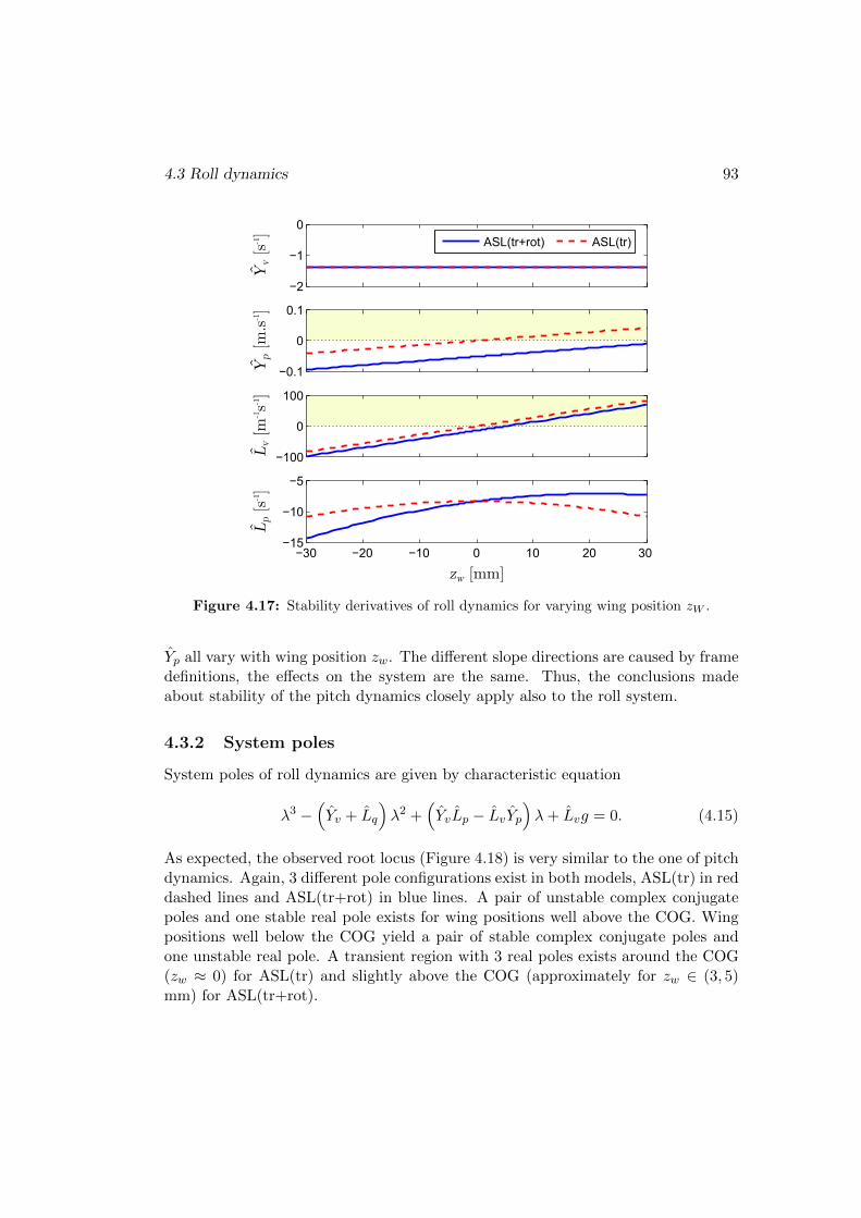
4.3 Roll dynamics 93
−2
−1
0
−0.1
0
0.1
−100
0
100
−15
−10
−5
ASL(tr+rot) ASL(tr)
Yv [s-1
]
Yp [m
.s-1]
L
v [m
-1s-1
]
Lp [s-1
]
−30 −20 −10 0 10 20 30
zw [mm]
Figure 4.17: Stability derivatives of roll dynamics for varying wing position zW .
Yp all vary with wing position zw. The different slope directions are caused by framedefinitions, the effects on the system are the same. Thus, the conclusions madeabout stability of the pitch dynamics closely apply also to the roll system.
4.3.2 System poles
System poles of roll dynamics are given by characteristic equation
λ3 −(Yv + Lq
)λ2 +
(YvLp − LvYp
)λ+ Lvg = 0. (4.15)
As expected, the observed root locus (Figure 4.18) is very similar to the one of pitchdynamics. Again, 3 different pole configurations exist in both models, ASL(tr) in reddashed lines and ASL(tr+rot) in blue lines. A pair of unstable complex conjugatepoles and one stable real pole exists for wing positions well above the COG. Wingpositions well below the COG yield a pair of stable complex conjugate poles andone unstable real pole. A transient region with 3 real poles exists around the COG(zw ≈ 0) for ASL(tr) and slightly above the COG (approximately for zw ∈ (3, 5)mm) for ASL(tr+rot).

94 4 Stability of near-hover flapping flight
−20 −15 −10 −5 0 5 10−10
−5
0
5
10
−20 −15 −10 −5 0 5 10−30
0
30
ASL (tr+rot)
ASL (tr)
Im (
λ)
z w [m
m]
Figure 4.18: Influence of wing position zw on the roll dynamics: pole positions in complexplane (top) and real part of the poles against the wing position (bottom).
The pole configuration in the pitch dynamics was determined by the derivativeMu, the pitch moment induced by longitudinal translation. In roll the importantderivative is Lv, the roll moment induced by the lateral translation. Assuming thederivative Yp is negligible and following the same steps as in pitch, the characteristicequation can be rewritten to
1 + Lvg
λ(λ− Yv
)(λ− Lp
) = 0, (4.16)
which is a root locus form with virtual feedback gain Lv. The root locus is shown inFigure 4.19. Because the numerator of the virtual open loop system is positive, thesituation is opposite to the pitch dynamics. We observe a pair of unstable complexpoles and a stable real pole for positive Lv, while negative Lv results into an unstablereal pole and a pair of stable complex poles.
However, because positive wing shoulder positions zw > 0 yield positive Lv, butnegative Mu, the difference in the root locus positive directions of pitch and of roll

4.3 Roll dynamics 95
Re (λ)
Im (
λ)
0
0
Lp Y
v
Lv → +∞
0
Lv → −∞
60°
120°
Lp + Y
v
3
^ ^
Figure 4.19: Root locus showing the effect of derivative Lv on the roll dynamics.
is compensated; for a given wing position zw the two systems behave similarly. Asmall region of stability exists in roll for small positive values of Lv, provided thatthe derivatives Yv and Lp remain negative. The stable region (with one fast realpole and a pair of slow lightly damped complex poles) can be enlarged by increasingthe damping of lateral translation or roll rotation. The roll can be damped similarto pitch: either passively by damping surfaces (tail, sails) or by an active feedback.
Due to the different predictions of the derivative Lv by the two models ASL(tr)and ASL(tr+rot) there exists an interval of positive wing positions, where ASL(tr)already predicts an unstable pair of complex poles and a stable real pole, whileASL(tr+rot) still gives a stable pair of complex poles and an unstable real pole.This can explain the discrepancy in the dronefly stability results (Section 3.4.3)among the considered models. Although the more complex models predict the poleconfiguration with an unstable real pole, the following section will show that theother configuration with an unstable complex pole-pair is more probable as it iseasier to control.
4.3.3 Active stabilization
The active stabilization of roll via rate feedback is analogous to pitch. A proportionalgain kp introduces a stabilizing moment L = −kpp. The characteristic equationbecomes
λ3 +(kp − Yv − Lp
)λ2 +
[Yv
(Lp − kp
)− LvYp
]λ+ Lvg = 0 (4.17)

96 4 Stability of near-hover flapping flight
and can be rewritten further while neglecting Yp as
1 + Lvg
λ(λ− Yv
)(λ+ kp − Lp
) = 0. (4.18)
The feedback gain moves the pole related to the roll rate damping towards minusinfinity which “opens” the root locus for positive values of Lv and enlarges the in-terval of stability.
The Routh-Hurwitz stability criterion yields three conditions(kp − Yv − Lp
) [Yv
(Lp − kp
)− LvYp
]− Lvg > 0 (4.19)
kp − Yv − Lp > 0 (4.20)
Lvg > 0. (4.21)
The third condition requires that Lv must be positive. The second condition isusually met as both derivatives Yv and Lp are typically negative. Finally, the firstcondition can be used to express the minimum gain value for stability. Assumingthe gain is positive we obtain
kp,min =LvYp − 2YvLp − Y 2
v +
√(Y 2v + LvYp
)2− 4YvLvg
−2Yv. (4.22)
4.4 Vertical and yaw dynamics stability
The vertical and yaw dynamics are decoupled from the rest of the dynamics (as longas Ixz = 0) and each can be treated separately. They are modelled by two first-orderdifferential equations
w = Zww + Zext (4.23)
r = Nrr + Next (4.24)
with coordinates according to Figure 4.20. The system poles can be expresseddirectly from the characteristic equation as
λw = Zw (4.25)
λr = Nr. (4.26)

4.4 Vertical and yaw dynamics stability 97
xB
zB
OB
Z
wr
N
Figure 4.20: Cordinates of vertical and yaw dynamics.↓αUpstroke
Δw
Downstroke↓FD
↓FL↓α↓FD
↓FL ↓Z
Δw
Figure 4.21: Effects of a disturbance in vertical direction ∆w. A decreased angle of attackin both upstroke and downstroke causes the cycle-averaged vertical force Z to drop, opposingthe disturbance.
For a stable system, the stability derivatives Zw and Nr need to be negative.
Figure 4.21 shows that a vertical disturbance ∆w decreases the angle of attack inboth upstroke and downstroke resulting into a drop of cycle-averaged vertical forceZ. Thus, the derivative Zw should be negative, representing a damping of the ver-tical motion.
The effect of a yaw disturbance ∆r on the wing aerodynamic forces is captured inFigure 4.22. In downstroke, the right wing moves in the sense of the disturbance,which increases the wing velocity and results into an increase of drag. The left wingmoves against the disturbance, which reduces the wing velocity and subsequently thedrag. Opposite situation can be observed in upstroke. Overall, the drag produced
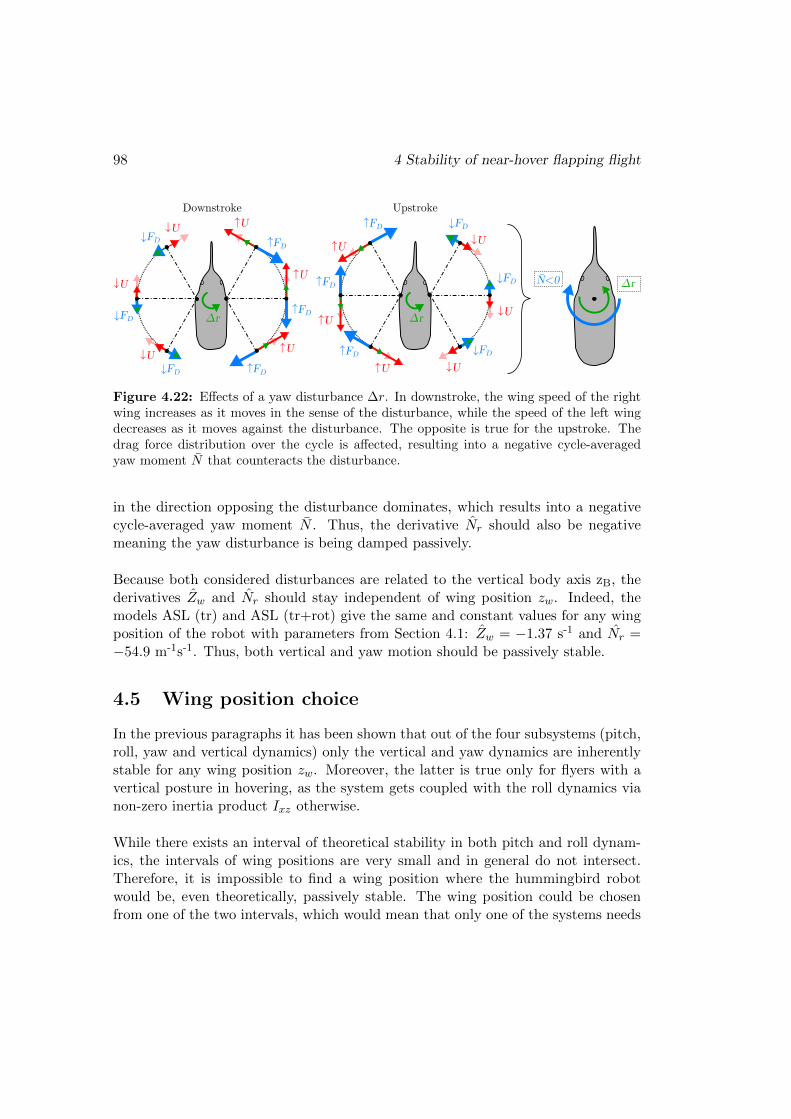
98 4 Stability of near-hover flapping flight
↓U↑U
UpstrokeDownstroke
Δr
↑FD ↑U
↑U
↓U
↓FD
↓U ↓U↑U
Δr↑U
↑U
↓U
↓U
ΔrN<0↓FD
↓FD
↓FD
↓FD
↓FD
↑FD
↑FD
↑FD
↑FD
↑FD
Figure 4.22: Effects of a yaw disturbance ∆r. In downstroke, the wing speed of the rightwing increases as it moves in the sense of the disturbance, while the speed of the left wingdecreases as it moves against the disturbance. The opposite is true for the upstroke. Thedrag force distribution over the cycle is affected, resulting into a negative cycle-averagedyaw moment N that counteracts the disturbance.
in the direction opposing the disturbance dominates, which results into a negativecycle-averaged yaw moment N . Thus, the derivative Nr should also be negativemeaning the yaw disturbance is being damped passively.
Because both considered disturbances are related to the vertical body axis zB, thederivatives Zw and Nr should stay independent of wing position zw. Indeed, themodels ASL (tr) and ASL (tr+rot) give the same and constant values for any wingposition of the robot with parameters from Section 4.1: Zw = −1.37 s-1 and Nr =−54.9 m-1s-1. Thus, both vertical and yaw motion should be passively stable.
4.5 Wing position choice
In the previous paragraphs it has been shown that out of the four subsystems (pitch,roll, yaw and vertical dynamics) only the vertical and yaw dynamics are inherentlystable for any wing position zw. Moreover, the latter is true only for flyers with avertical posture in hovering, as the system gets coupled with the roll dynamics vianon-zero inertia product Ixz otherwise.
While there exists an interval of theoretical stability in both pitch and roll dynam-ics, the intervals of wing positions are very small and in general do not intersect.Therefore, it is impossible to find a wing position where the hummingbird robotwould be, even theoretically, passively stable. The wing position could be chosenfrom one of the two intervals, which would mean that only one of the systems needs

4.6 Rate feedback gains 99
to be stabilized actively. However, even if the model predictions were correct, thepoles would still lie very close to the imaginary axis so some stability augmentationwould be necessary.
Since the flight needs to be stabilized in any case, a wing position should be chosenso that the controller can be as simple as possible yet robust. It has been shownthat if Mu is positive and Lv is negative, both pitch and roll systems have a pair ofcomplex unstable poles and a real stable pole. Such a system can be easily stabilizedby a simple rate feedback. On the other hand, negative Mu and positive Lv yieldsa pair of stable complex poles and an unstable real pole, a configuration that willremain unstable even with the rate feedback.
Re (λ)
Im (
λ)
0
0Re (λ)
Im (
λ)
0
0
zw ≫ 0
zw ≪ 0
OB
OB
→ not controllable by rate feedback → controllable by rate feedback
Figure 4.23: Pole configurations observed in both pitch and roll systems: situation forMu 0 or Lv 0 (wing positions well below the COG) cannot be stabilized by ratefeedback (left); situation for Mu 0 or Lv 0 (wing positions well above the COG) iscontrollable by rate feedback (right).
The quasi-steady based aerodynamic model predicts that positive Mu and negativeLv can only be obtained if the wing shoulders are placed (sufficiently high) abovethe COG. For the MAV considered in this chapter the wings should be placed abovezw > 5 mm (see Figures 4.8 and 4.17). To keep a certain safety margin, zw = 10mm was selected.
4.6 Rate feedback gains
The minimal necessary gains for stable pitch and roll rate feedback can be com-puted from equations (4.12) and (4.22), respectively. Considering zw = 10 mm we

100 4 Stability of near-hover flapping flight
will obtain kq,min ≈ 13.8 and kp,min ≈ 1.5. As expected, the pitch dynamics requireslightly higher gain as the chosen wing position is further from the passively stableinterval in pitch than in roll.
The root locus can be obtained by rewriting the characteristic equations 4.7 and4.17 (while neglecting Xq and Yp) into the following form
1 + kqλ(λ− Xu
)λ(λ− Xu
)(λ− Mq
)− Mug
= 0 (4.27)
1 + kpλ(λ− Yv
)λ(λ− Yv
)(λ− Lp
)+ Lvg
= 0. (4.28)
where the terms multiplied by the gains kq and kp are the open-loop transfer func-tions Q(s)/M(s) and P (s)/L(s), respectively. The root loci for gains kq and kp goingfrom zero to infinity are plotted in Figure 4.24. We can observe that, no matter howbig the gain is, the real part of the originally unstable pair of poles will always stay“trapped” between the pair of zeros, one at the origin and the other given by Xu
and Yv for pitch and roll, respectively. Thus, a more complex controller needs to beused if faster response is required. Alternatively, the derivatives Xu and Yv could bedecreased by adding passive damping surfaces. However, this would also influencethe remaining stability derivatives that define the open loop poles, so the effect onthe whole root locus is not apparent.
6
Im (
λ)
Re (λ)
4
2
0
-2
-4
-6
-20 -15 -10 -5 0 5
Pitch dynamics
6
Im (
λ)
Re (λ)
4
2
0
-2
-4
-6
-20 -15 -10 -5 0 5
Roll dynamics
Figure 4.24: Root locus for a rate feedback gain in pitch (left) and in roll systems (right).

4.7 Conclusion 101
4.7 Conclusion
The inherent instability of pitch and roll dynamics was demonstrated through a sim-plistic approach, which is coherent with quasi-steady modelling results. The systemscan be actively stabilized by a simple angular rate feedback, provided that the wingshoulders are placed sufficiently above the COG. This conclusion is in accordancewith morphology of hovering animals as well as with observations of basic motoricresponse in fruit-flies. Of course a more sophisticated control law can be used (andis probably used to some extent also by flying animals). The design of a controllerfor the hummingbird robot will be described in more detail in the next chapter.
4.8 References
B. Cheng and X. Deng. Translational and rotational damping of flapping flight andits dynamics and stability at hovering. IEEE Transactions on Robotics, 27(5):849–864, Oct. 2011. doi:10.1109/TRO.2011.2156170.
G. F. Franklin, J. Powel, and A. Emami-Naeini. Feedback Control of DynamicSystems. Prentice Hall, 4th edition, 2002.
L. Ristroph, G. Ristroph, S. Morozova, A. J. Bergou, S. Chang, J. Gucken-heimer, Z. J. Wang, and I. Cohen. Active and passive stabilization of bodypitch in insect flight. Journal of The Royal Society Interface, 10(85):1–13, 2013.doi:10.1098/rsif.2013.0237.
A. Sherman and M. H. Dickinson. Summation of visual and mechanosensory feed-back in drosophila flight control. Journal of Experimental Biology, 207(1):133–142,2004. doi:10.1242/jeb.00731.
M. Sun and Y. Xiong. Dynamic flight stability of a hovering bumblebee. Journal ofExperimental Biology, 208:447–459, 2005.
G. K. Taylor and H. G. Krapp. Sensory systems and flight stability: what doinsects measure and why? Advances in insect physiology, 34(231-316), 2008.doi:10.1016/S0065-2806(07)34005-8.
Y. Xiong and M. Sun. Dynamic flight stability of a bumblebee in forward flight.Acta Mech. Sinica, 24(1):25–36, Feb. 2008. doi:DOI 10.1007/s10409-007-0121-2.
Y. Zhang and M. Sun. Dynamic flight stability of a hovering model insect: theoryversus simulation using equations of motion coupled with navier-stokes equation.Acta Mech. Sinica, 26(4):509–520, 2010. doi:10.1007/s10409-010-0360-5.

102 References

Chapter 5
Flapping flight control
Since the hovering flapping flight is inherently unstable, it needs to be stabilizedpassively (by additional damping surfaces like tails or sails) or actively (by wingmotion). In this chapter an active attitude controller is developed based on thelinearised cycle-averaged model from the previous chapter. On top of that, a 4DOF flight controller is added to control the heading and the flight velocity in anydirection. Wing motion parameters suitable for thrust and control moment mod-ulation are selected. Finally, the controller performance is demonstrated throughsimulations with the full non-linear model from Chapter 3.
5.1 Control design
Many strategies of tail-less flapping flight control can be found in the literature. Ithas been demonstrated on a real insect-sized MAV that a simple angular rate feed-back succeeds to stabilize the attitude (Fuller et al., 2014), confirming the previouschapter conclusions. For flight control, most works use design techniques based onoutput or state feedback with decentralized (Doman et al., 2010) or centralized ar-chitectures (Deng et al., 2006b,a; Rifai et al., 2009; Rakotomamonjy et al., 2010; Maet al., 2013). Nevertheless, more elaborate control techniques have also been em-ployed (Chung and Dorothy, 2010). Most of the controllers were tested numericallyin non-linear simulations, often based on quasi-steady aerodynamics. However, thecontroller of Ma et al. (2013) succeeded to control near hover flight of a real insect-sized MAV inside a flight arena with a position tracking system.
The control design presented here uses the linearised model developed in the pre-vious chapters. The controllers are chosen and tuned by pole placement method.The MAV parameters were given in Section 4.1. According to the conclusions of theprevious chapter, the wing shoulders are placed at zw = 10 mm. Nevertheless, the
103

104 5 Flapping flight control
described approach should be applicable to any MAV with vertical body posture inhovering (Ixz = 0) and with wing shoulders placed sufficiently high above the COG.
The dynamics of such an MAV splits into 4 subsystems (pitch, roll, yaw and verticaldynamics) that can be treated separately. Pitch and roll dynamics are unstable,therefore the attitude is stabilized first. The second step is to control the flightvelocity (u, v, w) and the steering (r). In this section it is assumed that an arbitraryexternal moment and force can be applied on the MAV body. The generation ofthese control moments and forces by wing motion will be discussed in Section 5.2.From now on, the subscript ext of external efforts will be dropped, i.e. Lext = L,etc.
5.1.1 Pitch dynamics
The pitch dynamics has 2 DOFs: the pitch angle ϑ and the longitudinal velocity u.However, they do not need to be controlled independently. Similar to quadrocopters,e.g. Michael et al. (2010), the flight speed can be controlled by pitching the bodyforward and backward, which modulates the longitudinal component of the totalthrust vector. Thus, the pitch dynamics can be controlled through a single input,the pitch moment M , and the state space model (3.45) can be rewritten as a set oftransfer functions
U(s)
M(s)=
Xqs+ g
s3 − (Xu + Mq)s2 + (XuMq − MuXq)s− Mug(5.1)
Θ(s)
M(s)=
s− Xu
s3 − (Xu + Mq)s2 + (XuMq − MuXq)s− Mug. (5.2)
The system poles are given by the denominator roots. For wings placed above theCOG (zw > 0), the derivative Mu is negative, which results into a stable real poleand an unstable pair of complex-conjugate poles (see previous chapter). The zerosare given by the numerator roots and are different for the two transfer functions:z = −g/Xq for forward motion and z = Xu for pitch (another zero at z = 0 wouldappear for transfer function to pitch rate q due to derivation).
For the hummingbird robot parameters and zw = 10 mm we get the poles λ1 = −8.2and λ2,3 = 2.11±5.65i and zeros z = 215 for forward motion and z = −1.1 for pitch.The open loop pole-zero maps are displayed in Figure 5.1.
The proposed controller uses a cascade structure according to Figure 5.2. The in-nermost loop 1 controls the pitch rate q, the middle loop 2 controls the pitch angle ϑand the outer loop 3 controls the forward speed u. The first two loops can be imple-mented on-board of an MAV equipped with an Inertial Measurement Unit (IMU),

5.1 Control design 105
−50 0 50 100 150 200 250−6
−4
−2
0
2
4
6
U(s)/M(s) − open loop
Real Axis
Imag A
xis
−10 −5 0−6
−4
−2
0
2
4
6
Θ(s)/M(s) − open loop
Real Axis
Imag A
xis
Figure 5.1: Open loop pole-zero maps of pitch dynamics: forward motion (left) and pitchangle (right).
which senses the attitude and angular velocities. The third loop represents the pilotoperating the MAV or an autopilot, if an external measurement system like motiontracking or GPS is available. Each loop compensator was tuned by pole-placement,starting from the innermost loop. As it will be shown in Section 5.3, the output ofthe full non-linear model needs to be cycle-averaged to remove the oscillation dueto flapping from the feedback. This introduces a time delay not included in thelinearised model. Thus, an emphasis was put on keeping the phase margin large inorder to make the controller more robust.
It has been shown in the previous chapter that the pitch rate can be stabilized by arate feedback. However, much better performance is achieved by adding an integra-tor (cancelling the system zero at the origin) and a negative zero, i.e. a PI controller.The resulting root-locus and Bode plot for the selected gain are shown in Figure 5.3.Such a compensator reduces the steady state error and has a relatively high phasemargin of 77. The step response of the linear system is plotted in Figure 5.6 (left).The steady state error is still present but it will be compensated by the outer loops.
+-
M+-PI
uref +- PIP
q ϑ uQ(s)/M(s) 1/s
ϑref qref
LOOP 2LOOP 3
LOOP 1
U(s)/Θ(s)
Figure 5.2: Cascade control of pitch dynamics: loop 1 controls the pitch rate q, loop 2 thepitch angle ϑ and loop 3 the longitudinal velocity u.

106 5 Flapping flight control
102
101
100
101
360
180
0
P.M.: 77 degFreq: 4.99 Hz
Frequency (Hz)
Phase (
deg)
10
5
0
5
10
15
20
G.M.: 18 dB
Freq: 1.05 Hz
Magnitude (
dB
)
20 15 10 5 0 58
6
4
2
0
2
4
6
8
Real Axis
Imag A
xis
Figure 5.3: Loop 1 - pitch rate q: root locus (left) and Bode plot1 for the selected gain(right).
102
101
100
101
102
180
135
90
45
P.M.: 74.1 degFreq: 1.86 Hz
Frequency (Hz)
Phase (
deg)
60
40
20
0
20
40
G.M.: infFreq: Inf
Magnitude (
dB
)
15 10 5 050
40
30
20
10
0
10
20
30
40
50
Real Axis
Imag A
xis
Figure 5.4: Loop 2 - pitch angle ϑ: root locus (left) and Bode plot for the selected gain(right).
1In non-minimum phase systems (with poles/zeros in the right hand plane) the Bode plot followsless common rules and the stability condition gets modified. If an increasing gain brings the unstablesystem to stability and if its magnitude crosses 0 dB once, the stability criterion requires thatmagnitude is greater than 0 dB at −180 phase. The definitions of the gain and phase margins aremodified accordingly.

5.1 Control design 107
102
101
100
101
102
103
P.M.: 65.5 degFreq: 0.696 Hz
Frequency (Hz)
Phase (
deg)
150
100
50
0
50
G.M.: 14.3 dBFreq: 2.85 Hz
Magnitude (
dB
)
0 50 100 150 200 250 300
100
50
0
50
100
Real Axis
Imag A
xis
2 1.5 1 0.5 0
1
0.5
0
0.5
1
Imag A
xis
270
180
90
360
Figure 5.5: Loop 3 - longitudinal velocity u: root locus (top, left) with detail views(bottom) and Bode plot for the selected gain (top, right).
The output of the first closed loop is integrated to obtain the pitch angle ϑ, whichresults into an additional system pole at the origin. The second loop is controlledby a simple proportional feedback. The root locus and the Bode plot are shownin Figure 5.4. The phase margin is 74.1and the step response (Figure 5.6 centre)shows that closed loop system converges quickly to the desired value.
The output of the second closed loop is multiplied by the transfer function U(s)/Θ(s) =(Xqs+ g)/(s− Xu) to get the longitudinal speed u. Thus, the small negative zero ofthe pitch motion is cancelled and a large positive zero of forward motion is added.A PI controller (an integrator and a negative zero) is used to control u in the lastloop. The root locus and bode plot is shown in Figure 5.5. The chosen controllergain results into a phase margin of 65.5. The step response is displayed in Figure5.6 (right) showing a good performance with very little overshoot.

108 5 Flapping flight control
0 1 2 31
0
1
2
3x 10
3
0 1 2 31
0
1
2
3x 10
3
0 1 2 31
0
1
2
3x 10
3
0 1 2 30.5
0
0.5
1
1.5
0 1 2 32
0
2
4
6
8
0 1 2 32
0
2
4
0 1 2 30.5
0
0.5
1
1.5
0 1 2 30.5
0
0.5
1
1.5
0 1 2 30.2
0
0.2
0.4
0 1 2 32
0
2
4
6
8
0 1 2 32
0
2
4
6
8
0 1 2 30.5
0
0.5
1
1.5
Loop 1: qref = 1
xB
zB
OB
M
u
ϑ
q
Loop 2: ϑref = 1 Loop 3: uref = 1
u [m
.s-1]
ϑ [ra
d]
q [s-1
]M
[N
m]
time [s] time [s] time [s]
Figure 5.6: Step response of the linearized pitch dynamics in closed loop: loop 1 - pitchrate control (left), loop 2 - pitch angle control (center) and loop 3 - longitudinal speed control(right).

5.1 Control design 109
5.1.2 Roll dynamics
The control of the roll dynamics is nearly identical to pitch. The lateral flight speedis controlled by rolling the body left or right. Thus, only one input, the roll momentL, is considered. The system can be represented by a pair of transfer functions
V (s)
L(s)=
Yps− gs3 − (Yv + Lp)s2 + (YvLp − LvYp)s+ Lvg
(5.3)
Φ(s)
L(s)=
s− Yvs3 − (Yv + Lp)s2 + (YvLp − LvYp)s+ Lvg
. (5.4)
For wings well above the COG the denominator roots give one stable real pole andan unstable pair of complex-conjugate poles. Unlike in longitudinal direction, thelateral motion zero is negative, placed at z = g/Yp (derivative Yp is always neg-ative). The roll motion zero lies at z = Yv (another zero would lie at z = 0 fortransfer function to roll rate p). For the hummingbird robot parameters we getthe system poles λ1 = −9.2 and λ2,3 = 0.2 ± 3.8i and zeros z = −258 for lateralmotion and z = −1.4 for roll. The open loop pole-zero maps are shown in Figure 5.7.
V(s)/L(s) − open loop
−300 −250 −200 −150 −100 −50 0 50−4
−2
0
2
4
Real Axis
Imag A
xis
Φ(s)/L(s) − open loop
−10 −8 −6 −4 −2 0 2−4
−2
0
2
4
Real Axis
Imag A
xis
Figure 5.7: Open loop pole-zero maps of roll dynamics: sideways motion (left) and rollangle (right).
Again a cascade controller is used, where the innermost loop 1 controls the roll ratep, the middle loop 2 controls the roll angle ϕ and the outer loop 3 controls thelateral speed v (Figure 5.8). The compensators were chosen the same as in the pitchsystem: PI for loops 1 and 3 and P for loop 2. They were tuned by pole placement.

110 5 Flapping flight control
+-
L+-PI
vref +- PIP
p φ vQ(s)/M(s) 1/s
φref pref
LOOP 2LOOP 3
LOOP 1
U(s)/Θ(s)
Figure 5.8: Cascade control of roll dynamics: loop 1 controls the roll rate p, loop 2 thepitch angle ϕ and loop 3 the lateral velocity v.
102
101
100
101
360
270
180
90
P.M.: 83.4 degFreq: 3.34 Hz
Frequency (Hz)
Phase (
deg)
10
0
10
20
30
40
G.M.: 34.7 dB
Freq: 0.618 HzM
agnitude (
dB
)
15 10 5 0 55
4
3
2
1
0
1
2
3
4
5
Real Axis
Imag A
xis
Figure 5.9: Loop 1 - roll rate p: root locus (left) and Bode plot for the selected gain (right).
102
101
100
101
102
180
135
90
45
P.M.: 69 degFreq: 1.46 Hz
Frequency (Hz)
Phase (
deg)
80
60
40
20
0
20
40
G.M.: inf
Freq: Inf
Magnitude (
dB
)
15 10 5 030
20
10
0
10
20
30
Real Axis
Imag A
xis
Figure 5.10: Loop 2 - roll angle ϕ: root locus (left) and Bode plot for the selected gain(right).

5.1 Control design 111
101
100
101
102
103
270
225
180
135
90
P.M.: 77.4 degFreq: 0.423 Hz
Frequency (Hz)
Phase (
deg)
150
100
50
0
50
G.M.: 17.5 dB
Freq: 2.37 Hz
Magnitude (
dB
)
250 200 150 100 50 0
20
15
10
5
0
5
10
15
20
Real Axis
Imag A
xis
10 5 0
15
10
5
0
5
10
15
Real Axis
Imag A
xis
1.5 1 0.5 0
0.8
0.6
0.4
0.2
0
0.2
0.4
0.6
0.8
Real Axis
Imag A
xis
Figure 5.11: Loop 3 - lateral velocity v: negative root locus (top, left) with detail views(bottom) and Bode plot for the selected gain (top, right).
The root loci and the bode plots for the three loops are shown in Figures 5.9-5.11.The plots of loops 1 and 2 are equivalent to those in pitch. The loop 3, however,is different. A negative gain is required because the body needs to roll in negativeϕ direction to move in positive v direction and also both system zeros are negative.The phase margins of the loops 1, 2 and 3 are 83.4, 69and 77.4, respectively.
The step responses for all three compensators are plotted in Figure 5.12. The per-formance is comparable to the pitch system. The lateral speed response is slightlyslower due to a smaller gain, because a higher phase margin was preferred.

112 5 Flapping flight control
0 1 2 35
0
5
10
15x 10
4
0 1 2 3
0
10
20x 10
4
0 1 2 310
5
0
5x 10
4
0 1 2 30.5
0
0.5
1
1.5
0 1 2 32
0
2
4
6
8
0 1 2 33
2
1
0
1
0 1 2 30.5
0
0.5
1
1.5
0 1 2 30.5
0
0.5
1
1.5
0 1 2 30.4
0.2
0
0.2
0 1 2 38
6
4
2
0
2
0 1 2 38
6
4
2
0
2
0 1 2 30.5
0
0.5
1
1.5
Loop 1: pref = 1 Loop 2: φref = 1 Loop 3: vref = 1
time [s] time [s] time [s]
v [m
.s-1]
φ [ra
d]
p [s-1
]L [N
m]
OB
yB
zB
φ
vp
L
Figure 5.12: Step response of the linearized roll dynamics in closed loop: loop 1 - roll ratecontrol (left), loop 2 - roll angle control (center) and loop 3 - lateral speed control (right).
5.1.3 Yaw and vertical dynamics
The yaw dynamics is a SISO (single input single output) system that can be repre-sented by the transfer function from yaw moment N to yaw rate r

5.1 Control design 113
R(s)
N(s)=
1
s− Nr
. (5.5)
Because Nr is negative, the system pole λ = Nr is always stable (see Section 4.4).For the considered MAV parameters we get λ = −54.9. While the yaw could becontrolled by a simple proportional feedback, a pure integral feedback results intoa zero steady state error. The root locus showing the selected gain and the closedloop step response are displayed in Figure 5.13 (left).
The vertical dynamics is also a SISO system with a transfer function from verticalforce Z to vertical speed w
W (s)
Z(s)=
1
s− Zw. (5.6)
The system is also passively stable, because the derivative Zw is negative, but theaerodynamic damping is much smaller than in yaw (λ = −0.027 for the consideredMAV). Thus, a PI compensator is used for vertical speed control. The root locusand step response are shown in Figure 5.13 (right).
−60 −50 −40 −30 −20 −10 0−20
−15
−10
−5
0
5
10
15
20
Real Axis
Imag A
xis
Yaw rate
−12 −10 −8 −6 −4 −2 0−5
0
5
Real Axis
Imag A
xis
Vertical speed
time [s]
r [s
-1]
0 0.05 0.1 0.15 0.2 0.250
0.5
1
w [
m.s
-1]
0 0.2 0.4 0.6 0.80
0.5
1
time [s]
Figure 5.13: Root locus (top row) and step response (bottom row) of the yaw rate (left)and vertical speed (right) controllers. The vertical speed system pole is very close to theorigin and so it is overlapped by the integrator pole in the root locus.

114 5 Flapping flight control
5.1.4 Complete controller
The scheme of the complete controller with all 4 subsystems is shown in Figure5.14. The right dashed rectangle highlights the attitude controller, the velocitycontroller is inside the dashed rectangle on the left and represents the (auto)pilot.The compensator parameters are summarized in Table 5.1.
+-
M+-PI
uref +- PIP
q ϑ uQ(s)/M(s) 1/s U(s)/Θ(s)
ϑref
+-
ZPI
wrefw
qref
+-
NI
rrefr
+-
L+-PI
vref +- PIP
p φ vP(s)/L(s) 1/s V(s)/Φ(s)
φref pref
W(s)/Z(s)
R(s)/N(s)
VELOCITY CONTROL ATTITUDE CONTROL LINEARISED DYNAMICS
Figure 5.14: Cascade control of the linearised system.
Transfer function KP KI
q 0.0003s+ 10
s0.0003 0.003
Pitch dynamics ϑ 10 10 -
u 0.5s+ 1.3
s0.5 0.65
p 0.0002s+ 10
s0.0002 0.002
Roll dynamics ϕ 9 9 -
v -0.3s+ 1.2
s-0.3 -0.36
Yaw dynamics r 0.0031
s- 0.003
Vertical dynamics w 0.3s+ 5
s0.3 1.5
Table 5.1: Control parameters: the compensator transfer function and an equivalent PIcontroller with a proportional gain KP and an integral gain KI .

5.2 Control moment generation 115
5.2 Control moment generation
The proposed controller can stabilize the attitude and control the flight in 4 DOF bymodulating an external vertical force Z and moments around the three body axesL, M and N . In reality, these control efforts need to be generated through changesof wing kinematics.
5.2.1 Control derivatives
As it was already presented in Section 3.2.1, the effects of the wing motion parameterchanges ∆p on the generated efforts are given by the control derivatives matrix Jdefined as
J =
Xp1 Xp2 · · · Xpn
Yp1 Yp2 · · · Ypn...
.... . .
...Np1 Np2 · · · Npn
. (5.7)
Each matrix element represents a partial derivative of a cycle averaged force / mo-ment component with respect to one of the wing motion parameters, pi. The deriva-tives are calculated in the equilibrium with states xe and wing motion parameters
pe; a shortened notation is used as in the previous sections, i.e. Xpi = ∂X∂pi
(xe,pe).
The wing motion parameter changes ∆p, necessary to generate the desired combi-nation of forces and moments, can be computed by relation
∆p = J+[X,Y, Z, L,M,N ]T , (5.8)
where J+ is a pseudo-inverse of the matrix J. Finally, these changes are added tothe equilibrium values
p = pe + ∆p. (5.9)
The control derivatives were evaluated numerically using the approach described inSection 3.2.2, assuming the set of wing kinematics parameters p according to Sec-tion 3.1.1. The results are split into two parts. First, we change the parameterssymmetrically, i.e. the parameter changes made on both wings are equal and haveidentical signs. Second, we change the parameters asymmetrically, i.e. the changesdone on the two wings have equal magnitudes but opposite signs.

116 5 Flapping flight control
When applying the wing kinematic changes symmetrically (subscript S) only thelongitudinal system efforts (X, Z and M) are modified. The linearised relationshipcan be written as
[X,Z,M ]T = JS [φmS , φ0S , αmS , α0S , ϕαS , δm1S , δm2S , βS , fS ]T . (5.10)
The matrix JS was normalized to have comparable values between the forces andmoments: the row belonging to the moment M was divided by a characteristiclength RCP = Rr2 (the CP position on the wing). The normalized matrix withunits mN/, or mN/Hz in case of the flapping frequency, was evaluated as
JS =
φmS φ0S αmS α0S ϕαS δm1S δm2S βS fS
X 0 0.59 0 −4.8 0 0.29 0 −3.4 0Z 4.9 0 1.4 0 −0.6 0 4.3 0 15MRCP
0 −2.5 0 −0.41 0 2.9 0 −0.44 0
. (5.11)
For asymmetric changes of wing kinematics (subscript A) only the lateral systemforce and moments Y , L and N are affected. The relationship can be written as
[Y,L,N ]T = JA [φmA, φ0A, αmA, α0A, ϕαA, δm1A, δm2A, βA]T , (5.12)
where the control derivatives matrix, normalized as before, is
JA =
φmA φ0A αmA α0A ϕαA δm1A δm2A βA
Y −0.66 0 0.31 0 1.9 0 −0.29 0L
RCP−4.3 0 −2 0 0.47 0 −7.2 0
NRCP
0 0.2 0 −7.8 0 0.094 0 −3.8
. (5.13)
By studying the matrices JS and JA we can identify two groups of parameters ac-cording to their effect on the generated forces and moments. The first group includesflapping frequency f , sweep amplitude φm, angle of attack amplitude αm, phase shiftϕα and amplitude of figure eight-like deviation δm2 (Figure 5.15 left). If we modifythese parameters symmetrically on both wings, we control the vertical force Z. Ifwe modify these parameters, excluding the flapping frequency, asymmetrically (withpositive sign on the left wing and negative on the right wing) we modulate the rollmoment L and lateral force Y .
The second group includes sweep angle offset φ0, angle of attack offset α0, amplitudeof oval-like deviation δm1 and mean stroke plane inclination β (Figure 5.15 right).Symmetric changes of these parameters result into pitch moment M and longitu-dinal force X modulation. Same parameters taken asymmetrically modify the yawmoment N .

5.2 Control moment generation 117
ϕm
δm2αm
βδm1
ϕ0
αm+α0
αm-α0
Δsymmetric → Z
Δasymmetric → L & Y
Δsymmetric → M & X
Δasymmetric → N
flapping frequency
f
phase shiftφα
Figure 5.15: Wing kinematics parameters, split into two groups according to their effecton the cycle averaged forces: parameters affecting Z, L and Y (left) and M , X and N(right).
5.2.2 Choice of control parameters
In the MAV design the number of parameters needed for control needs to be min-imized. The matrices (5.11) and (5.13) show that two parameters modified sym-metrically and two modified asymmetrically are sufficient to generate independentlythe four control forces/moments Z, L, M and N . While this leaves no control ofthe ”parasite” forces X and Y , it allows a simpler design of the MAV wing motioncontrol mechanism. Another two parameters, one symmetric and one asymmetric,would be necessary to assure that X and Y is zero.
For the selected 4 parameters (pS1 controlling Z, pS2 controlling M , pA1 controllingL and pA2 controlling N) the control derivatives matrix reduces to Jred and thecontrol force and moments can be expressed as
ZMLN
= Jred
∆pS1
∆pS2
∆pA1
∆pA2
=
ZpS1 0 0 0
0 0 LpA1 00 MpS2 0 00 0 0 NpA2
∆pS1
∆pS2
∆pA1
∆pA2
. (5.14)

118 5 Flapping flight control
The relationship shows that the control system is, in theory, fully decoupled. Finally,the control force and moments are transformed into the wing kinematic parametersas
[∆pS1,∆pS2,∆pA1,∆pA2]T = J−1red[X,L,M,N ]T . (5.15)
There are many possible choices of the control parameters set. Since the effect onX and Y forces is ignored, a successful control is not guaranteed. Thus, the controlperformance of each selected combination needs to be tested in a non-linear simu-lation. Finally, the choice of the control parameters is heavily constrained by thedesign feasibility of the wing motion control mechanism.
Because the designed MAV is powered by a DC motor, the flapping frequency can becontrolled easily. It was chosen as the symmetric parameter controlling the verticalforce Z. The choice of the remaining parameters reflects the control mechanism thatwill be presented in Section 7.2 and is sketched in Figure 5.16. The roll momentL is controlled by asymmetric modulation of the flapping amplitude φm, the pitchmoment M by symmetric modulation of the mean wing position (offset) φ0 and theyaw moment by asymmetric modulation of the offset φ0.
L (roll) M (pitch) N (yaw)
−Δϕm +Δϕm −Δϕ0 −Δϕ0 +Δϕ0 −Δϕ0
Figure 5.16: Control moments generated through wing kinematics parameters φm and φ0.
5.3 Simulation results
Figure 5.17 shows the control scheme with the full, non-linear model that has beenimplemented in Matlab/Simulink. The model includes the non-linear aerodynamicsand body dynamics from Chapter 3. A moving average over the last wingbeat isused to remove the periodic oscillation due to flapping from the feedback. To testthe controller performance, a trajectory with step commands in all four controlledDOFs (velocities u,v,w, angular velocity r) was used. First a step input was appliedsuccessively on each DOF, one at a time, to show the control performance with thecoupling effects of the rest of the nonlinear system. Then, the step input was appliedto all the 4 DOFs at once to reveal any control cross-coupling effects and evaluate

5.3 Simulation results 119
VELOCITY CONTROL
+-
AERO-
DYNAMICS
+
BODY
DYNAMICS
M
Z
w
ϑ
u
+-
PI
+-
PI
CONTROL
DERIVATIVES
MATRIX
J+
Δp
wref
uref
+- L
N
+-
PI
+-
rref
vref
I
v
r
φ
wingkinematicsparameters
p
q+-
+-
PI
PI
P
P
ATTITUDE CONTROL
u
w
v
r
φ
ϑ q
p
CYCLE
AVERAGING
CYCLE
AVERAGING
++
p0
Figure 5.17: Cascade control of the full non-linear system.
the potential decrease of control performance. The control commands were set to0.1 m/s and 10/s for the linear and angular velocities, respectively, representingslow flight around hovering.
The simulation results are shown in Figure 5.18 where the green solid lines repre-sent the full non-linear model, the black dotted lines the linearised model and thered dashed lines the command. Unlike in the linearised model, there exists smallcoupling between the pitch and vertical dynamics and between the roll and yawdynamics in the non-linear model. Nevertheless, the longitudinal (pitch + verticaldynamics) and lateral (roll + yaw dynamics) systems stay independent.
The high frequency oscillation in the longitudinal DOFs (u, w, ϑ) of the non-linearsystem is caused by the periodic aerodynamic forces due to the wing flapping. Themean values, however, are closely following the linear results. In the lateral DOFs(v, r, ϕ) the oscillation appears only when the left and right wing kinematics or flowconditions differ. It is in particular pronounced during the lateral motion, wherean asymmetrically varying wing drag induces high yaw oscillation (see Figure 4.13).Yet again, the non-linear system response is reasonably close to the linearised model.
The time behaviour of the control parameters (Figure 5.19) shows that the neces-sary changes in the wing kinematics are very small. The vertical flight controllervaries the flapping frequency f by approximately ±2 Hz. The lateral flight controlrequires changes of flapping amplitude φm by only ±0.5. The wing offset φ0 is usedfor both longitudinal flight and yaw control. While variation of ±1.5 is enoughfor longitudinal speed control, up to ±4 is required for yaw rotation. This is in

120 5 Flapping flight control
0 2 4 6 8 10 12 14 16 18 20
0.1
0
0.1
0 2 4 6 8 10 12 14 16 18 20
0
0.05
0.1
0 2 4 6 8 10 12 14 16 18 20
0.05
0
0.05
0.1
0.15
0 2 4 6 8 10 12 14 16 18 2040
20
0
20
40
0 2 4 6 8 10 12 14 16 18 20
2
1
0
1
0 2 4 6 8 10 12 14 16 18 205
0
5
0 2 4 6 8 10 12 14 16 18 20
0
20
40
Longit
udin
al
speed
u [m
.s-1]
Lateral
speed
v [m
.s-1]
Vertic
al
speed
w [m
.s-1]
Yaw
rate
r [°.s
-1]
Roll
angle
φ [°]
Pit
ch
angle
ϑ [°]
Yaw
angle
ψ [°]
Time [s]
Full model Command Linear model
Individualsteps
Combinedsteps
Figure 5.18: Simulation results: response to a sequence of step inputs and a combinedstep in the 4 controlled DOFs (u, v, w and r). Comparison of the full, non-linear modelwith the cycle-averaged linearised model.
.

5.3 Simulation results 121
0 2 4 6 8 10 12 14 16 18 20
24
26
28
0 2 4 6 8 10 12 14 16 18 20
79.5
80
80.5
0 2 4 6 8 10 12 14 16 18 20−5
0
5left right
Fla
ppin
g
frequency
f [H
z]
Fla
ppin
g
am
plitude
ϕm [°]
Fla
ppin
g
offset
ϕ0 [°]
Time [s]
Figure 5.19: Simulation results: wing kinematic parameters controlling the flight duringthe test sequence in Figure 5.18.
0 2 4 6 8 10 12 14 16 18 20
0.05
0
0.05
0 2 4 6 8 10 12 14 16 18 20
0.1
0
0.1
0 2 4 6 8 10 12 14 16 18 200.04
0.02
0
0.02
0.04
Roll m
om
ent
L [m
Nm
]
Time [s]
Pit
ch m
om
ent
M [m
Nm
]
Yaw
mom
ent
N [m
Nm
]
Figure 5.20: Simulation results: estimates of cycle averaged control moments generatedby the wings during the test sequence in Figure 5.18.

122 References
accordance with the control derivatives matrix (5.13), which shows that the effect ofφ0 on yaw moment N is relatively low. A more effective parameter for yaw controlcould be chosen, but a solution using the same parameter for both pitch and rollwas preferred as it reduces the MAV design complexity. No significant change inthe overall performance is observed in the combined command and also the wingkinematics parameters remain in a similar range.
Figure 5.20 displays the control moments generated by the wings with the modifiedwing kinematics. They were obtained by averaging the wing aerodynamic effortsover each flapping cycle while removing the component due to aerodynamic damping(estimated by the linearised model). Their maximum absolute values are |L|max ≈0.05 mNm (roll), |M |max ≈ 0.13 mNm (pitch) and |N |max ≈ 0.04 mNm (yaw).
5.4 Conclusion
The controller of near-hover flapping flight presented in this chapter can stabilizeand control the flight in 4 DOF by altering 4 parameters: the flapping frequency, thedifference between the left and right wing flapping amplitude and, independently,the left and right wing offset. The controller was tuned for the linearised, cycle-averaged model. Its performance was tested in a non-linear simulation that showedgood agreement between the two models. The study provides an initial estimate ofthe necessary wing kinematics changes as well as of control moments these changesshould generate. A prototype designed based on these results will be presented inthe following chapters.
5.5 References
S. Chung and M. Dorothy. Neurobiologically inspired control of engineered flappingflight. Journal of Guidance, Control, and Dynamics, 33(2):440–453, 2010.
X. Deng, L. Schenato, and S. Sastry. Flapping flight for biomimetic robotic insects:part II-flight control design. IEEE Transactions on Robotics, 22(4):789–803, Aug.2006a. doi:10.1109/TRO.2006.875483.
X. Deng, L. Schenato, W. C. Wu, and S. S. Sastry. Flapping flight for biomimeticrobotic insects: part I-system modeling. IEEE Transactions on Robotics, 22(4):776–788, Aug. 2006b. doi:10.1109/TRO.2006.875480.
D. B. Doman, M. W. Oppenheimer, and D. O. Sigthorsson. Wingbeat shape modula-tion for flapping-wing micro-air-vehicle control during hover. Journal of Guidance,Control, and Dynamics, 33(3):724–739, 2010. doi:10.2514/1.47146.

References 123
G. F. Franklin, J. Powel, and A. Emami-Naeini. Feedback Control of DynamicSystems. Prentice Hall, 4th edition, 2002.
S. B. Fuller, M. Karpelson, A. Censi, K. Y. Ma, and R. J. Wood. Controlling freeflight of a robotic fly using an onboard vision sensor inspired by insect ocelli.Journal of The Royal Society Interface, 11(97), 2014. doi:10.1098/rsif.2014.0281.
K. Y. Ma, P. Chirarattananon, S. B. Fuller, and R. J. Wood. Controlledflight of a biologically inspired, insect-scale robot. Science, 340:603–607, 2013.doi:10.1126/science.1231806.
N. Michael, D. Mellinger, Q. Lindsey, and V. Kumar. The GRASP Multi-ple Micro UAV Testbed. IEEE Robotics and Automation, 17(3):56–65, 2010.doi:10.1109/MRA.2010.937855.
T. Rakotomamonjy, M. Ouladsine, and T. L. Moing. Longitudinal modelling andcontrol of a flapping-wing micro aerial vehicle. Control engineering practice, 18(7):679–690, Jul. 2010. doi:10.1016/j.conengprac.2010.02.002.
H. Rifai, J.-F. Guerrero-Castellanos, N. Marchand, and G. Poulin. Bounded at-titude control of a flapping wing micro aerial vehicle using direct sensors mea-surements. In 2009 IEEE International Conference on Robotics and Automation,Kobe, Japan, pages 3644–3650. 2009 IEEE International Conference on Roboticsand Automation, Kobe, Japan, 2009.

124 References

Chapter 6
Flapping mechanism
While the theoretical basis of the hovering flapping flight has been introduced inthe previous text, the remaining chapters are dedicated to the robotic humming-bird design. Our project aims at a tail-less flapping wing MAV with a wingspan ofaround 20 cm and a mass around 20 g. This chapter presents the development of anuncontrolled robot prototype generating the lift force, consisting of a flapping mech-anism and a pair of wings. Details are given on its design as well as on conductedexperiments that lead to a successful tethered take-off demonstration.
6.1 Flapping mechanism concept
The lift production is crucial for any air vehicle. The designed hummingbird-likerobot generates the lift by flapping its wings. They need to be driven at a frequencythat is high enough to counteract the gravity and stay airborne. There are manyways how to obtain the flapping motion - the design of the transmission mechanismdepends strongly on the actuator choice. The vast majority of existing MAV designsemployed rotary electric motors (e.g. de Croon et al., 2009; Keennon et al., 2012).However, other actuators were also used, including piezo-actuators (Wood, 2008),SMA actuators (Furst et al., 2013), magnetic actuators (Vanneste et al., 2011) andeven combustion engines (Zdunich et al., 2007).
In this project an electric DC motor was chosen for three main reasons:
1. There is a relatively wide choice of electric motors in the 2 g to 7 g range (10 %to 35 % of expected total weight).
2. DC motors can be directly powered by off-the-shelf speed controllers and Li-Pobatteries.
125
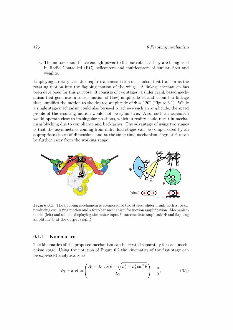
126 6 Flapping mechanism
3. The motors should have enough power to lift our robot as they are being usedin Radio Controlled (RC) helicopters and multicopters of similar sizes andweights.
Employing a rotary actuator requires a transmission mechanism that transforms therotating motion into the flapping motion of the wings. A linkage mechanism hasbeen developed for this purpose. It consists of two stages: a slider crank based mech-anism that generates a rocker motion of (low) amplitude Ψ, and a four-bar linkagethat amplifies the motion to the desired amplitude of Φ = 120 (Figure 6.1). Whilea single stage mechanism could also be used to achieve such an amplitude, the speedprofile of the resulting motion would not be symmetric. Also, such a mechanismwould operate close to its singular positions, which in reality could result in mecha-nism blocking due to compliance and backlashes. The advantage of using two stagesis that the asymmetries coming from individual stages can be compensated by anappropriate choice of dimensions and at the same time mechanism singularities canbe further away from the working range.
θΨ
Φ
"slot" ≡
Figure 6.1: The flapping mechanism is composed of two stages: slider crank with a rockerproducing oscillating motion and a four-bar mechanism for motion amplification. Mechanismmodel (left) and scheme displaying the motor input θ, intermediate amplitude Ψ and flappingamplitude Φ at the output (right).
6.1.1 Kinematics
The kinematics of the proposed mechanism can be treated separately for each mech-anism stage. Using the notation of Figure 6.2 the kinematics of the first stage canbe expressed analytically as
ψ3 = arctan
A1 − L1 cos θ −√L2
2 − L21 sin2 θ
L3
+π
2, (6.1)

6.1 Flapping mechanism concept 127
where θ is the input angle and ψ3 is the angle of the intermediary link 3-4. Theanalytic solution of the second (amplification) stage is a classical solution of a fourbar mechanism
φ = arctan(ab
)− arccos
(c√
a2 + b2
), (6.2)
where
a = −2L4L6 sin (ψ3 − α34)
b = 2A2L6 − 2L4L6 cos (ψ3 − α34) (6.3)
c = L25 −A2
2 − L24 − L2
6 + 2A2L4 cos (ψ3 − α34) .
The dimensions were optimized numerically by minimizing a cost function, whichconsisted of a difference from the desired amplitude and a difference between up-stroke and downstroke velocity profiles; the final dimensions are in Table 6.1. Therelationship of the output angle φ on the input angle θ is very close to a harmonicfunction (Figure 6.3).
Figure 6.2: Kinematic scheme of the flapping mechanism.
L1 L2 L3 L4 L5 L6 A1 A2 α34
2.25 12.00 8.00 14.00 7.53 3.57 11.00 -9.20 -70
Table 6.1: Mechanism dimensions (lengths in mm, angles in )
The final structure of the flapping mechanism was rearranged (compared to Figure6.2) to minimize the overall mechanism dimensions. The mutual orientation of thetwo stages was adapted as is shown in Figure 6.1 and the wing bar was connected
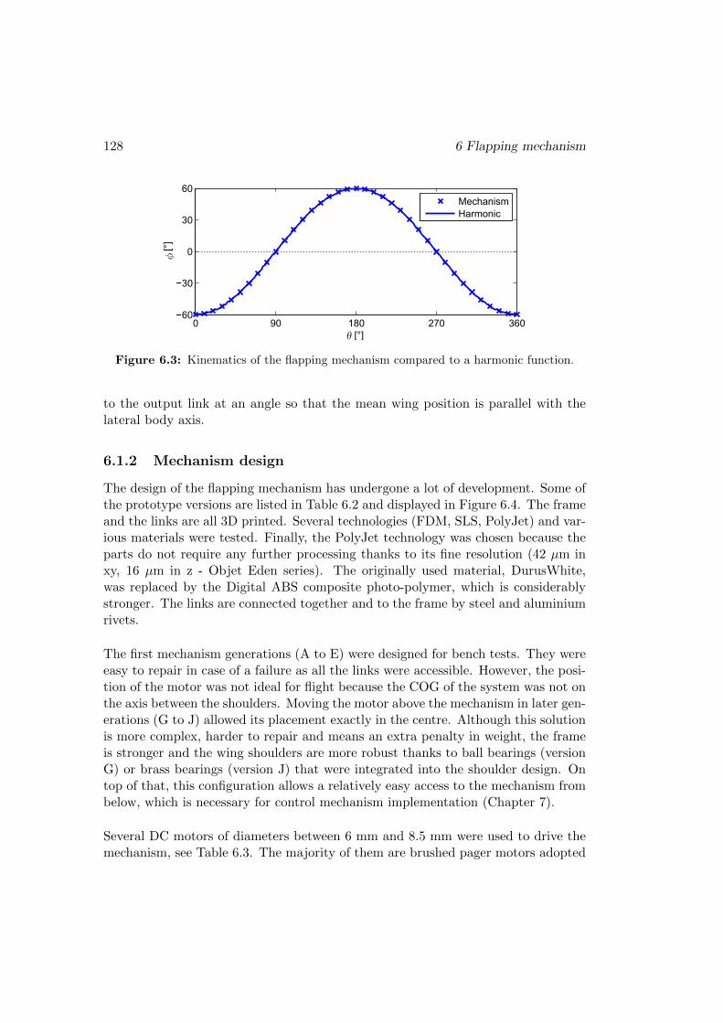
128 6 Flapping mechanism
0 90 180 270 36060
30
0
30
60
[°]
[°]
Mechanism
Harmonic
ϕ
θ
Figure 6.3: Kinematics of the flapping mechanism compared to a harmonic function.
to the output link at an angle so that the mean wing position is parallel with thelateral body axis.
6.1.2 Mechanism design
The design of the flapping mechanism has undergone a lot of development. Some ofthe prototype versions are listed in Table 6.2 and displayed in Figure 6.4. The frameand the links are all 3D printed. Several technologies (FDM, SLS, PolyJet) and var-ious materials were tested. Finally, the PolyJet technology was chosen because theparts do not require any further processing thanks to its fine resolution (42 µm inxy, 16 µm in z - Objet Eden series). The originally used material, DurusWhite,was replaced by the Digital ABS composite photo-polymer, which is considerablystronger. The links are connected together and to the frame by steel and aluminiumrivets.
The first mechanism generations (A to E) were designed for bench tests. They wereeasy to repair in case of a failure as all the links were accessible. However, the posi-tion of the motor was not ideal for flight because the COG of the system was not onthe axis between the shoulders. Moving the motor above the mechanism in later gen-erations (G to J) allowed its placement exactly in the centre. Although this solutionis more complex, harder to repair and means an extra penalty in weight, the frameis stronger and the wing shoulders are more robust thanks to ball bearings (versionG) or brass bearings (version J) that were integrated into the shoulder design. Ontop of that, this configuration allows a relatively easy access to the mechanism frombelow, which is necessary for control mechanism implementation (Chapter 7).
Several DC motors of diameters between 6 mm and 8.5 mm were used to drive themechanism, see Table 6.3. The majority of them are brushed pager motors adopted

6.1
Fla
pp
ing
mech
anism
concep
t129
Ver. Date Material MotoraMotor Mechanism Total Max. Wing FlappingWeight Weight Weight Lift Length Frequency
[g] [g] [g] [g] [mm] [Hz]
A 2/2012 FDM ABS A-6 1.77 3.43 5.2 - - -C2 5/2012 DurusWhite A-6 1.77 4.03 5.8 6.4 70 21.1E2 10/2012 DurusWhite D-7 2.78 4.72 7.5 9.6 70 23.5E4 1/2014 Digital ABS F-8 5.20 4.90 10.1 16.1 90 26.2
G2 4/2013 DurusWhite A-7 2.69 6.28 9.0 9.6 70 24.5J2 1/2014 Digital ABS F-8 5.20 7.30 12.5 16 90 23.8
Table 6.2: Evolution of the flapping mechanism. aSee Table 6.3 for motor details.
A C2 E4
G2 J2
Figure 6.4: Evolution of the flapping mechanism - generations A (2/2012) to J (1/2014).

130 6 Flapping mechanism
by RC modellers (BR DC), but professional brushless motors (BL DC) were alsosuccessfully used. The factors limiting the maximal speed of small DC motors areusually the temperature (the motor is heated by current and friction) and, in caseof brushed motors, the wear of the brushes. It is the latter case that also limits thelifetime of the brushed motors.
The highest lift was obtained with the 8mm BL DC from Faulhaber. Its advantageis that the performance remains constant over time, but it needs to be driven bya speed controller whose stock version (SC 1801P) is too large and heavy (23 mmx 32 mm, 3.6 g). Thus, a smaller and lighter speed controller needs to be eitherfound on the market or developed to use this motor in flight. An alternative motor,giving nearly the same performance, is the 8.5 mm BR DC from AEO-RC. Theperformance, however, decreases with time as the motor heats up. The motor lastsonly about 5 minutes when operated at the maximal flapping frequency before itsbrushes wear out. Currently, the BL motor is used for bench tests and the BR motorfor take-off demonstrations.
A two stage gearbox is used to reduce the motor speed. The limited space requiresthat gears with a small module of 0.3 mm are used. The choice of the reductionratio was limited by the gears available on the market. The final gearbox consistsof a 9t pinion, 40t/9t double spur gear and 40t spur gear giving a reduction ratio ofapproximately 19.75:1. A custom built gear set with a gear ratio optimized for theload and motor characteristic combination is being considered.
An exploded view of the most recent flapping mechanism (version J) is shown inFigure 6.5. Its weight, without the motor, is 7.3 g.
6.1.3 Wing design
The design of the wings is inspired by the Nano Hummingbird (Keennon et al., 2012)and by the DelFly (de Croon et al., 2009). The wing is made of a thin flat mem-brane. It has two sleeves, one on the leading edge and one on the root edge (close tothe body), that accommodate the leading edge and root edge CFRP (carbon-fibre-reinforced polymer) bars. Since the angle between the sleeves is greater than theangle between the bars the wing becomes cambered and twisted after the assembly(Figure 6.6). The camber is bistable - it flips passively from one side to anotherdepending on the direction of motion, as can be seen in Figure 6.7.
The wings are hand built - a reasonable accuracy and repeatability is achieved byprinting the desired shape on a sheet of paper that is attached under the membrane

6.1 Flapping mechanism concept 131
Motor Typem D L kV R Pmax
+
[g] [mm] [mm] [rpm/V] [Ω] [W]
A-6 BR* AEO-RC GPS6 1.77 6 14 13000 2.8 1.2
A-7 BR* AEO-RC GPS7 2.69 7 16 11000 2.1 1.5
A-8 BR* AEO-RC EPS8 4.85 8.5 20 12600 0.7 2.5
D-7 BR* Didel MK07-1.7 2.78 7 17 11000 2.1 1.6F-8 BL Faulhaber 0824-006B 5.20 8 24 5753 3.1 > 2.5
Table 6.3: DC motors used along the project. BR = brushed motor, BL = brushlessmotor. All motors have output shaft of 1 mm in diameter. *No data-sheets provided,parameters estimated experimentally. +Maximal output power achieved during experimentswith flapping prototype E4 without motor overheating (approximate values).
DC Motor
Motor adapter(optional)
Brass bearings
Leading edge bar
Root edge bar
Top frame
Bottom frame
Gearbox
Flapping mechanism
Connecting rivets
Shoulder hinge axis
Motor pinion
Figure 6.5: Exploded view of the flapping mechanism J2.

132 6 Flapping mechanism
BoPET (Mylar) Polyester (Icarex) CFRP
Figure 6.6: Polyester film wing becomes cambered after assembly.
0 ms 2 ms 4 ms 6 ms 8 ms 10 ms
Figure 6.7: High speed camera sequence of a wing flipping at the stroke reversal (top view)while flapping at 15 Hz. The whole sequence represents about 15 % of the flapping cycle.
and used as a template for cutting. The best results (in terms of lift and durability)were obtained with a 15 micron thick polyester film. 1 mm x 0.12 mm CFRP bandsare used as stiffeners. The sleeves at the leading edge and at the root edge arereinforced with Icarex to increase their durability. They allow an easy assembly anddisassembly as well as free rotation around the 0.8 mm leading edge and 0.5 mmroot edge CFRP bars.
In the early prototypes the whole wing frame, including the leading edge and rootedge bars, was mobile, as displayed in Figure 6.8 (left). An adapted version ofthis solution has an adjustable angle between the leading edge and root edge bars(Figure 6.8 centre) and is used to find an optimal angle between the sleeves. Finallythe design was simplified and the mass being moved reduced by fixing the root bardirectly to the frame, making it coincident with the wing shoulder axis (Figure 6.8right).

6.2 Experiments 133
Figure 6.8: Different solutions of the wing frame: mobile root bar (left), mobile root barwith adjustable angle (center), fixed root bar (right).
6.2 Experiments
Many tests were carried out throughout the development process. While the maingoal was to maximize the generated lift force by mechanism and wing design opti-misations, mechanism reliability and wing robustness were also important factors.A high speed camera (Photron FASTCAM SA3, resolution 1024 x 1024 pixels) wasused to observe the wing behaviour throughout the cycle and to track the mecha-nism and wing kinematics. The generated forces were measured on a custom builtforce balance.
6.2.1 Wing kinematics
While the flapping mechanism was designed for a nominal flapping amplitude Φ0 =120, the amplitude will increase with frequency due to compliance of the wing barsand of the mechanism itself. The high speed camera was employed to quantify these
ϕroot R
ϕR
xB
yB
Figure 6.9: Definition of the tracked angles.

134 6 Flapping mechanism
effects as well as to identify any imperfections compared to the mechanism theoret-ical kinematics.
The sweep angle was tracked at the wing root (φroot) and at the wing tip (φtip, seeFigure 6.9). The camera was set to record at 2000 fps with a shutter speed of 10000 fps to remove any motion blur. The amplitude was subsequently calculated asΦ = φmax− φmin and offset as φ0 = (φmax + φmin)/2, where φmax and φmin are themaximal and minimal observed angles φ, respectively.
Figure 6.10 shows the traces of wing angles of prototype E4 over two wingbeatsat a flapping frequency of 25Hz. The increase of the tracked flapping amplitudecompared to the theoretical model is significant. The amplitude measured at thewing roots includes the effect of backlashes in the linkage mechanism as well as thecompliance of its links. The compliance of the leading edge bars results into a fur-ther amplification of the amplitude, measured at the wing tip. It can be observedthat the bars flex in particular during the stroke reversal when the accelerations arehigh. Thus, the sweep angle at the wing tip becomes more triangular compared tothe theoretical, nearly harmonic curve.
0 0.25 0.5 0.75 1 1.25 1.5 1.75 2
90
60
30
0
30
60
90
Wingbeat [ ]
Sw
eep a
ngle
[°]
Flapping frequency: 25 Hz
tip R
tip L
root R
root L
theory
Figure 6.10: Tracked wing kinematics of prototype E4 at f = 25 Hz. Left wing traces arein blue, right wing traces in red. The sweep angle was measured at the wing tip (φtip) andat the output of the mechanism (φroot). Black dash-dotted line represents the theoreticalkinematics, without compliance and backlashes.

6.2 Experiments 135
t=0ms
t=20mst=20ms
0 1
2
3
4
5
6
78
01
2
3
4
5
67 8
t=40ms
t=20mst=20ms
16 1514
13
12
11
10
9889
10
11
12
13
14
15
DOWNSTROKE
UPSTROKE
Figure 6.11: High speed camera measurement: the image displays the wings every 2.5 msover one complete cycle at 25 Hz. The sequence is split into the downstroke (frames 0 → 8,top) and the upstroke (frames 8→ 16, bottom).

136 6 Flapping mechanism
The small differences in the left and right wing amplitudes are caused by the mech-anism imperfections. There is, however, a small difference in the timing of the wingreversal, which is an inherent property coming from the design of the joints betweenthe slider crank stage and the amplification stages. The right wing reverses beforethe left wing when behind the body (φ > 0), while the opposite happens in frontof the body (φ < 0). This can produce a small oscillation around the yaw axis,nevertheless, the effects should average out over one wingbeat.
A composite image of high speed camera frame sequence showing the wing positionsevery 2.5 ms over the full wingbeat is shown in Figure 6.11. We can observe theleading edge bar deformation close to the reversal, the differences between upstrokeand downstroke of left and right wing as well as the positions of mechanism jointsthroughout the wingbeat.
The relationship between the flapping amplitude and offset and the flapping fre-quency is displayed in Figure 6.12. For the measured range of frequencies (15 to25 Hz) the mechanism amplitude increases from above 140 to almost 150. Theincrease of the wing tip amplitude is more significant, from below 160 to almost180. As will be shown in Section 6.2.3, this can be considered as beneficial, be-cause an increase of flapping amplitude means a lower frequency is needed to takeoff and a lower frequency means lower accelerations and lower inertial forces on themechanism links.
15 20 25
140
150
160
170
180
Frequency [Hz]
Fla
ppin
g a
mplit
ude
[°]
wingtip R
wingtip L
wingroot R
wingroot L
Φ
15 20 250
2
4
6
8
10
Frequency [Hz]
Mean w
ing p
ositio
n
[°]
wingtip R
wingtip L
wingroot R
wingroot L
ϕ0
Figure 6.12: The tracked flapping amplitude (left) and offset (right) as a function offlapping frequency. Results measured for prototype E4.

6.2 Experiments 137
The offset remains slightly positive and nearly constant in the studied range (around4 on the left and between 4 and 7 on the right wing); there is almost no differencebetween the wing roots and tips. The small non-zero offset does not represent amajor problem. The generated pitch moment can be compensated by a small shiftof the prototype COG.
6.2.2 Force balance
Measuring the efforts of a flapping wing robot is a challenging task. The generatedforces are relatively small (order of 0.01 N) which requires high sensitivity. On topof that these efforts are of a periodic nature where not only the flapping frequencybut also the higher harmonics are present. Hence the sensor should have a highresonance frequency.
The most frequently used commercial 6DOF force-torque sensor in the flapping wingresearch is the Nano17 Titanium (ATI, 2014). It is the only sensor on the marketthat is compact and has a high sensitivity to forces (resolution up to 1/682 N ≈0.15 g) and moments (resolution up to 3/364 mNm ≈ 0.008 mNm) while keeping ahigh resonance frequency in all DOFs (3 kHz). However, its price was well above theproject budget so a decision was made to build a custom force balance. To keep thedesign simple the balance should be able to measure only lift Z and pitch momentM . Moreover, only the cycle averaged efforts were of our primary interest.
In the past we already used a precision pocket scale to evaluate the mean lift withacceptable results. The sensors used in the scales are usually double beam can-tilevers with strain gages in full bridge configuration. Their advantage is that theyare insensitive to the axial force as well as to the bending moment. The experimen-tally determined resonance frequency of a sensor extracted from one of the scaleswas 210 Hz, roughly 8 times the flapping frequency of the robot prototype. That isnot enough to measure the time histories within one flapping cycle, but sufficient toevaluate the cycle averaged values. Thus these sensors were selected as inexpensiveyet reasonably precise base components for the designed force balance.
The balance uses two of these single axis force sensors in a configuration that isshown in Figure 6.13. Applying lift FL, drag FD and moment M on the balanceresults in the following sensor forces
S1 = (FDH −M)/B − FL/2S2 = (M − FDH)/B − FL/2 (6.4)
Rx = −FD.

138 6 Flapping mechanism
Figure 6.13: Schematics of the force balance (left) and its free body diagram (right).
Originally a third sensor was used to measure the drag force FD. However, thefirst tests showed that the cycle averaged drag force was very low and its effecton the moment was negligible. Thus the third sensor has been dismounted for themeasurements presented here. This allows to mount the robot closer to the rotationjoints, which increases the resonant frequency of the whole system. The moment atthe robot COG, M , is approximated by the moment at the centre between the tworotation joints, MC . The measured efforts can be expressed as
FL = −S1 − S2
MC = M − FDH = (S2 − S1)B/2. (6.5)
The sensitivity of sensors 1 and 2 to the moment can be tuned by the selection ofdistance B between the two sensor joints. It was set to 50 mm, giving a good sensi-tivity yet enough space in between to fix the robot prototype. For small distance Hand small cycle averaged drag force FD the moment MC is a good approximation ofthe true moment M , with an error that can be expressed from equation (6.5). Thishas no effect on the lift force precision.
The assembled force balance is shown in Figure 6.14. Each sensor is connected toa custom build electronic circuit that provides stabilized power to the bridge andamplifies the bridge output. The sensors have been calibrated one at a time. Therotational joints in the system should have as little friction as possible. The jointon the left is constructed as a blade inside a groove. The joint is held together bya magnetic force of a NdFeB cylindrical magnet that attracts the blade inside thegroove. Both the blade and the groove are from soft magnetic steel. The joint onthe right is built in a similar manner. Since it should also allow displacement to thesides to have an isostatic system, the blade was replaced by a steel ball that is touch-ing a flat steel plate. Since the contact of the spherical ball and flat plate is onlyin one point, another magnet was attached on the top to increase the attractive force.

6.2 Experiments 139
Steelblade
Steelgroove
Magnet Magnet
Steelplate
Steelball
Sensor 1 Sensor 2
Sensor 1Sensor 2
Flapper attachment
Tested prototype
Amplifiers
Figure 6.14: Force balance overview and detail views on sensors and magnetic joints
The force balance signals are processed with a dSpace 1103 digital signal proces-sor, together with the voltage and current readings of the DC motor. The flappingfrequency can be detected from the motor current, because the motor torque is con-stantly changing due to the periodic aerodynamic and inertial forces. Nevertheless,the setup is also equipped with an optional infrared barrier providing a trigger signalat every wing pass. In case of the brushless DC the frequency is calculated from thesignals of Hall sensors, which are integrated in the motor.
The measured resonant frequency of the balance is 173 Hz for lift and 297 Hz forpitch moment (Figure 6.15). As expected, this is too low to measure detailed forceand moment traces over a flapping cycle, but the system provides enough bandwidthto evaluate the cycle averages for the expected flapping frequencies (below 30 Hz).
50 100 150 200 250 300 350 40010
20
30
40
50
Frequency [Hz]
Magnitude [
dB
]
Lift force
fpeak = 173 Hz
flappingfrequency
50 100 150 200 250 300 350 40010
20
30
40
50
Frequency [Hz]
Magnitude [
dB
]
Pitch moment
fpeak = 297 Hz
flappingfrequency
Figure 6.15: Force balance: measured frequency response gain magnitude of lift (left) andmoment (right) showing the resonance frequencies.
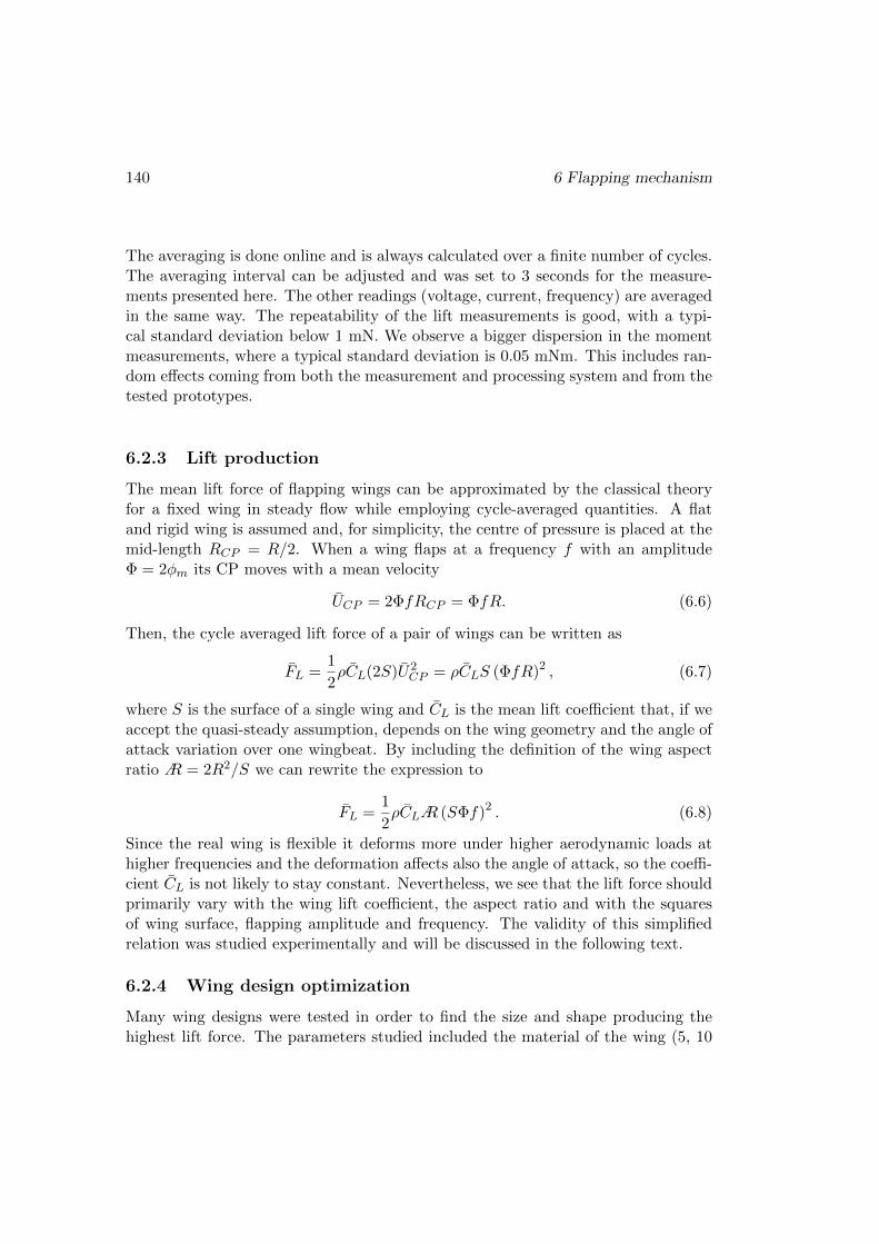
140 6 Flapping mechanism
The averaging is done online and is always calculated over a finite number of cycles.The averaging interval can be adjusted and was set to 3 seconds for the measure-ments presented here. The other readings (voltage, current, frequency) are averagedin the same way. The repeatability of the lift measurements is good, with a typi-cal standard deviation below 1 mN. We observe a bigger dispersion in the momentmeasurements, where a typical standard deviation is 0.05 mNm. This includes ran-dom effects coming from both the measurement and processing system and from thetested prototypes.
6.2.3 Lift production
The mean lift force of flapping wings can be approximated by the classical theoryfor a fixed wing in steady flow while employing cycle-averaged quantities. A flatand rigid wing is assumed and, for simplicity, the centre of pressure is placed at themid-length RCP = R/2. When a wing flaps at a frequency f with an amplitudeΦ = 2φm its CP moves with a mean velocity
UCP = 2ΦfRCP = ΦfR. (6.6)
Then, the cycle averaged lift force of a pair of wings can be written as
FL =1
2ρCL(2S)U2
CP = ρCLS (ΦfR)2 , (6.7)
where S is the surface of a single wing and CL is the mean lift coefficient that, if weaccept the quasi-steady assumption, depends on the wing geometry and the angle ofattack variation over one wingbeat. By including the definition of the wing aspectratio A = 2R2/S we can rewrite the expression to
FL =1
2ρCLA (SΦf)2 . (6.8)
Since the real wing is flexible it deforms more under higher aerodynamic loads athigher frequencies and the deformation affects also the angle of attack, so the coeffi-cient CL is not likely to stay constant. Nevertheless, we see that the lift force shouldprimarily vary with the wing lift coefficient, the aspect ratio and with the squaresof wing surface, flapping amplitude and frequency. The validity of this simplifiedrelation was studied experimentally and will be discussed in the following text.
6.2.4 Wing design optimization
Many wing designs were tested in order to find the size and shape producing thehighest lift force. The parameters studied included the material of the wing (5, 10
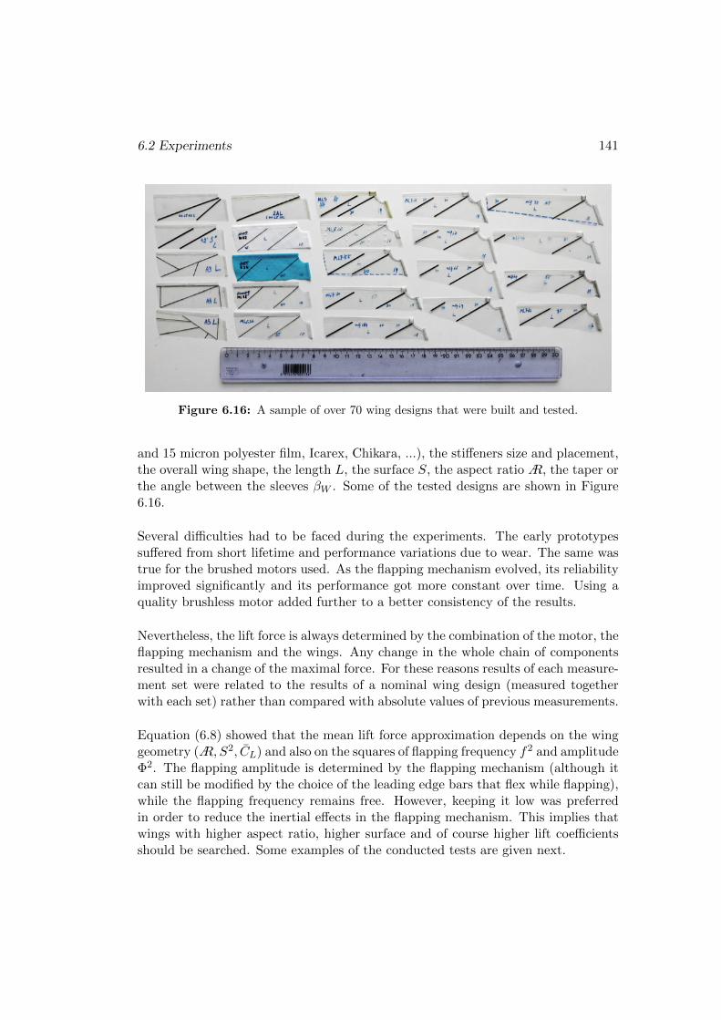
6.2 Experiments 141
Figure 6.16: A sample of over 70 wing designs that were built and tested.
and 15 micron polyester film, Icarex, Chikara, ...), the stiffeners size and placement,the overall wing shape, the length L, the surface S, the aspect ratioA, the taper orthe angle between the sleeves βW . Some of the tested designs are shown in Figure6.16.
Several difficulties had to be faced during the experiments. The early prototypessuffered from short lifetime and performance variations due to wear. The same wastrue for the brushed motors used. As the flapping mechanism evolved, its reliabilityimproved significantly and its performance got more constant over time. Using aquality brushless motor added further to a better consistency of the results.
Nevertheless, the lift force is always determined by the combination of the motor, theflapping mechanism and the wings. Any change in the whole chain of componentsresulted in a change of the maximal force. For these reasons results of each measure-ment set were related to the results of a nominal wing design (measured togetherwith each set) rather than compared with absolute values of previous measurements.
Equation (6.8) showed that the mean lift force approximation depends on the winggeometry (A, S2, CL) and also on the squares of flapping frequency f2 and amplitudeΦ2. The flapping amplitude is determined by the flapping mechanism (although itcan still be modified by the choice of the leading edge bars that flex while flapping),while the flapping frequency remains free. However, keeping it low was preferredin order to reduce the inertial effects in the flapping mechanism. This implies thatwings with higher aspect ratio, higher surface and of course higher lift coefficientsshould be searched. Some examples of the conducted tests are given next.
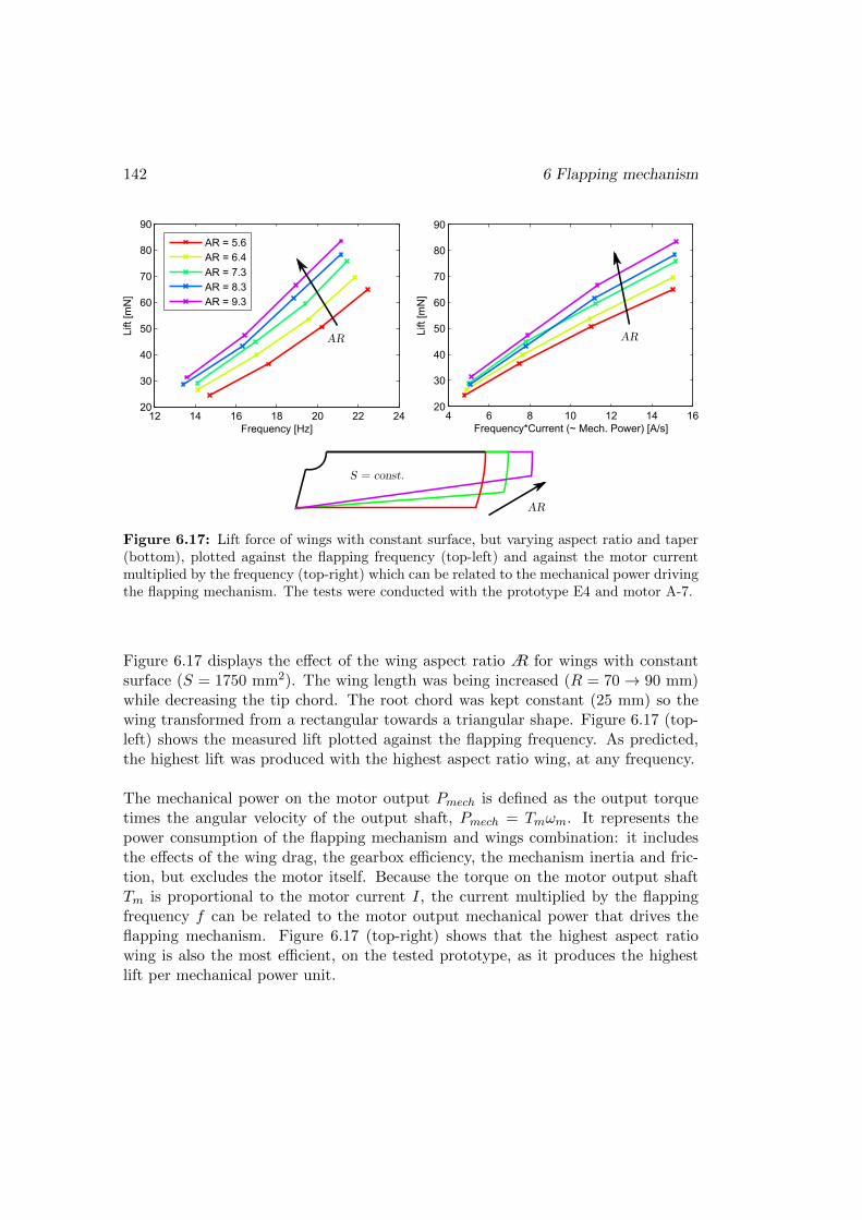
142 6 Flapping mechanism
4 6 8 10 12 14 1620
30
40
50
60
70
80
90
Frequency*Current (~ Mech. Power) [A/s]Lift
[mN
]12 14 16 18 20 22 24
20
30
40
50
60
70
80
90
Frequency [Hz]
Lift
[mN
]
AR = 5.6
AR = 6.4
AR = 7.3
AR = 8.3
AR = 9.3
AR
S = const.
AR AR
Figure 6.17: Lift force of wings with constant surface, but varying aspect ratio and taper(bottom), plotted against the flapping frequency (top-left) and against the motor currentmultiplied by the frequency (top-right) which can be related to the mechanical power drivingthe flapping mechanism. The tests were conducted with the prototype E4 and motor A-7.
Figure 6.17 displays the effect of the wing aspect ratio A for wings with constantsurface (S = 1750 mm2). The wing length was being increased (R = 70→ 90 mm)while decreasing the tip chord. The root chord was kept constant (25 mm) so thewing transformed from a rectangular towards a triangular shape. Figure 6.17 (top-left) shows the measured lift plotted against the flapping frequency. As predicted,the highest lift was produced with the highest aspect ratio wing, at any frequency.
The mechanical power on the motor output Pmech is defined as the output torquetimes the angular velocity of the output shaft, Pmech = Tmωm. It represents thepower consumption of the flapping mechanism and wings combination: it includesthe effects of the wing drag, the gearbox efficiency, the mechanism inertia and fric-tion, but excludes the motor itself. Because the torque on the motor output shaftTm is proportional to the motor current I, the current multiplied by the flappingfrequency f can be related to the motor output mechanical power that drives theflapping mechanism. Figure 6.17 (top-right) shows that the highest aspect ratiowing is also the most efficient, on the tested prototype, as it produces the highestlift per mechanical power unit.

6.2 Experiments 143
10 15 20 25 3020
40
60
80
100
120
140
160
Frequency [Hz]
Lift
[mN
]
S = 1750 mm2
S = 2054 mm2
S = 2382 mm2
0.58 0.6 0.62 0.64 0.66 0.68
20
40
60
80
100
120
140
160
Motor efficiency [−]
Lift
[mN
]
S
AR = const.
SS
Figure 6.18: Lift force of wings with constant aspect ratio, but varying surface. Themeasured lift is plotted against the flapping frequency (top-left) and against the efficiency ofthe motor driving the flapping mechanism (top-right). The tests were terminated when themotor recommended heat limit was reached. The tests were conducted with the prototypeE4 and motor F-8.
The effect of the wing area S on the lift force should be even more pronounced asit appears in the approximation in the second power. The experimental results forwings of constant aspect ratio (A = 9.3) are shown in Figure 6.18. The surface wasbeing increased while preserving the overall shape. Indeed, for a constant frequency,the highest lift was produced by the largest wing (Figure 6.18 top-left).
All the wings produce comparable amount of lift per mechanical watt. To includealso the electric drive, the lift is this time plotted against the motor efficiency ηmdefined as the ratio between the mechanical and electrical power
ηm =PmechPel
=TmωmUI
, (6.9)
where U and I are the motor voltage and current, respectively. Figure 6.18 (top-right) shows that the most efficient wing with the used drive (BL DC Faulhaber0824) is the smallest wing. On top of that, this allows to reach a higher mechanicalpower without a risk of motor overheating and thus also a higher absolute lift, al-though at a cost of increased flapping frequency. These results show that the wingsneed to be optimized for every new combination of motor and flapping mechanismin order to achieve maximal efficiency, which will be crucial for flight endurance.

144 6 Flapping mechanism
βw = 16°
30° cmin = 14 mm
L = 90 mm
cmax = 25 mm
30°
Figure 6.19: Shape and dimensions of the wing producing the highest lift. Its aspect ratiois A = 9.3.
90 mm32 mm
Faulhaber0824
Figure 6.20: Prototype J2 with the best wing producing almost 160 mN of lift at 24 Hz.
It needs to be said that not all the tests were as conclusive as those presented here.The effects of the stiffeners placement were much more subtle. Some results wouldeven contradict previous findings due to differences among the used motors and pro-totypes. Nevertheless, the experimental approach lead to a gradual lift increase.
The highest generated lift so far, almost 160 mN ≈ 16 g, was produced with thewings with dimensions shown in Figure 6.19 attached to the mechanism J2 drivenby the 8 mm brushless motor F-8 (Figure 6.20). The measured lift curve is plottedin Figure 6.21. The grey dash-dotted line represents a trend-line assuming the liftforce FL is proportional to the second power of frequency f , while the lift coef-ficient CL and flapping amplitude Φ in equation (6.8) remain constant. The realmeasured curve scales with slightly higher power, because the flapping amplitudealso increases with frequency (see Figure 6.12) and the lift coefficient changes dueto wing flexibility. Nevertheless, this shows that FL ≈ const.f2 can be used as a(conservative) rule of thumb when extrapolating the results.

6.2 Experiments 145
5 10 15 20 250
20
40
60
80
100
120
140
160
Frequency [Hz]
Lift
[mN
]
ftake-off
= 21.5 Hz
prototype weight 12.5 g
FL
* = const.f 2
0 1 2 3 40
20
40
60
80
100
120
140
160
Power [W]Lift
[mN
]
mechanical power
electrical power
Figure 6.21: Measured lift of the best wing: relationship on the flapping frequency (left)and on the mechanical and electrical power of the motor (right). The black dotted line dis-plays the prototype weight, grey dash-dotted line is a fitted curve assuming FL = const.f2.Individual measurements are plotted with crosses, the lines connect the average values.
The force necessary to lift the prototype weight (12.5 g) is displayed by the blackdotted line, showing that the prototype would take-off around f = 21.5 Hz. How-ever, the power source is still off-board and the prototype lacks any control.
Due to the hovering flapping flight inherent instability, a take-off was demonstratedwith a help of guide-wire that fixes the prototype attitude, but allows a free move-ment along the vertical axis as well as free yaw rotation (Figure 6.22). Older proto-
Figure 6.22: Take-off demonstration: a guide wire was used to stabilize the attitude ofthe uncontrolled prototype E4. Power was off-board, brought by 200 microns thin copperwires and controlled by hand to maintain a constant altitude after the take-off. Time ofeach frame is displayed in the upper left corner.

146 References
type E4 was used for this test, because it was easier to attach it to the guide wire.The power was still off-board and was brought by 200 microns thin copper wires.A control mechanism needed for active stabilization is being developed and will bedescribed in the next chapter.
6.3 References
ATI Industrial Automation. Nano17 titanium. https://www.ati-ia.
com/products/ft/ft_models.aspx?id=Nano17+Titanium, 2014. Accessed:18/08/2014.
G. de Croon, K. de Clerq, R. Ruijsink, B. Remes, and C. de Wagter. Design,aerodynamics, and vision-based control of the DelFly. International Journal ofMicro Air Vehicles, 1(2):71–97, Jun. 2009. doi:10.1260/175682909789498288.
S. J. Furst, G. Bunget, and S. Seelecke. Design and fabrication of a bat-inspiredflapping-flight platform using shape memory alloy muscles and joints. Smart Ma-terials and Structures, 22(1):014011, 2013. doi:10.1088/0964-1726/22/1/014011.
M. T. Keennon, K. R. Klingebiel, H. Won, and A. Andriukov. Development ofthe nano hummingbird: A tailless flapping wing micro air vehicle. AIAA paper2012-0588, pages 1–24, 2012.
T. Vanneste, A. Bontemps, X. Q. Bao, S. Grondel, J.-B. Paquet, and E. Cattan.Polymer-based flapping-wing robotic insects: Progresses in wing fabrication, con-ception and simulation. In ASME 2011 International Mechanical EngineeringCongress and Exposition, pages 771–778. American Society of Mechanical Engi-neers, 2011.
R. J. Wood. The first takeoff of a biologically inspired at-scale roboticinsect. IEEE Transactions on Robotics, 24(2):341–347, Apr. 2008.doi:10.1109/TRO.2008.916997.
P. Zdunich, D. Bilyk, M. MacMaster, D. Loewen, J. DeLaurier, R. Kornbluh, T. Low,S. Stanford, and D. Holeman. Development and testing of the Mentor flapping-wing micro air vehicle. Journal of Aircraft, 44(5):1701–1711, 2007.

Chapter 7
Control mechanism
The primary role of the flapping wings is the thrust production. In a tail-less designthe wings have a second, yet equally important, role: the active flight stabilizationand control. To stabilize the body attitude and to steer, the wings need to generatemoments around the three body axes: roll moment L around xB, pitch moment Maround yB and yaw moment N around zB axis.
To produce the control moments the robot needs to be able to modulate the meanlift and drag forces of each wing independently and also to control the placement ofthe cycle-averaged lift force with respect to the centre of gravity, see Figure 7.1. Insuch case the roll moment can be generated through a difference between the meanlift force of the left and of the right wing. The pitch moment can be produced byplacing the mean lift force of both wings in front of or behind the centre of gravity.Finally, the yaw moment can be generated by a difference between the mean dragof the left and of the right wing.
xB
OB
M
2FL
yB
zB
L
stroke plane
↑FL
↓FL
yB
xB
N−FD
+FD
Roll moment Pitch moment Yaw moment
stroke plane
zB
Figure 7.1: Principle of control moment generation. FL and FD are cycle averaged liftand drag forces, respectively, generated by a single wing.
147

148 7 Control mechanism
Two possible solutions of the control mechanism, published in (Karasek et al., 2013,2014), are presented in the following text. The first is based on the wing twistmodulation according to Keennon et al. (2012). The second generates the necessarymoments by modulating the wing flapping amplitude and offset (mean position),a strategy similar to Ma et al. (2013) and Truong et al. (2014).
7.1 Moment generation via wing twist modulation
The wing design presented in Section 6.1.3 consists of a membrane attached betweenthe leading edge and root edge bars. At rest the membrane is slightly loose. Thewing becomes cambered and twisted when moved due to a pressure difference. Fora wing with specifically optimized geometry (Figure 7.2 left), the lift force can beincreased by moving the root bar away from the membrane (membrane is stretched,γ > 0) and decreased by moving it towards the membrane (membrane is loosened,γ < 0 in Figure 7.2 right). This concept is used in the Nano Hummingbird and iscalled the Variable Wing Twist Modulation (Keennon et al., 2012).
γ
γ
Figure 7.2: Wing twist modulation principle adapted from Keennon et al. (2012) (left)and measurement of lift as a function of angle γ for various flapping frequencies (right).
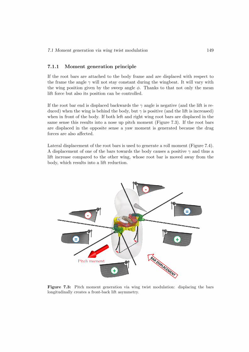
7.1 Moment generation via wing twist modulation 149
7.1.1 Moment generation principle
If the root bars are attached to the body frame and are displaced with respect tothe frame the angle γ will not stay constant during the wingbeat. It will vary withthe wing position given by the sweep angle φ. Thanks to that not only the meanlift force but also its position can be controlled.
If the root bar end is displaced backwards the γ angle is negative (and the lift is re-duced) when the wing is behind the body, but γ is positive (and the lift is increased)when in front of the body. If both left and right wing root bars are displaced in thesame sense this results into a nose up pitch moment (Figure 7.3). If the root barsare displaced in the opposite sense a yaw moment is generated because the dragforces are also affected.
Lateral displacement of the root bars is used to generate a roll moment (Figure 7.4).A displacement of one of the bars towards the body causes a positive γ and thus alift increase compared to the other wing, whose root bar is moved away from thebody, which results into a lift reduction.
Figure 7.3: Pitch moment generation via wing twist modulation: displacing the barslongitudinally creates a front-back lift asymmetry.
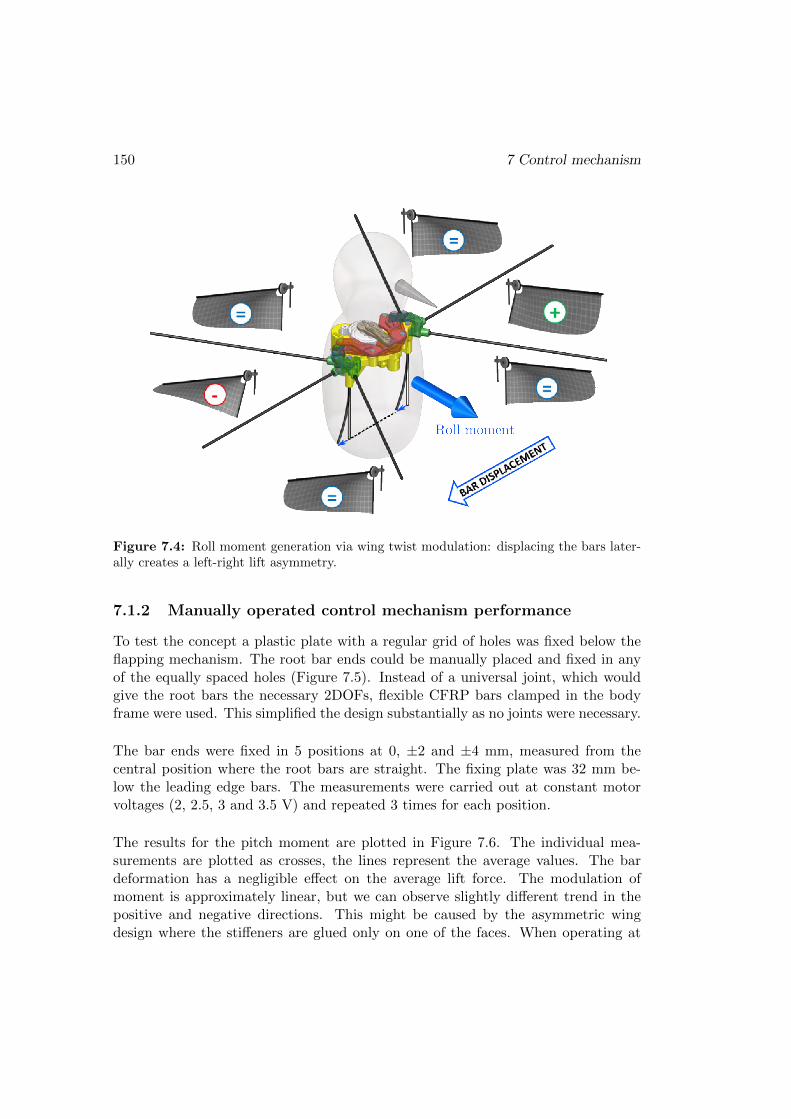
150 7 Control mechanism
Figure 7.4: Roll moment generation via wing twist modulation: displacing the bars later-ally creates a left-right lift asymmetry.
7.1.2 Manually operated control mechanism performance
To test the concept a plastic plate with a regular grid of holes was fixed below theflapping mechanism. The root bar ends could be manually placed and fixed in anyof the equally spaced holes (Figure 7.5). Instead of a universal joint, which wouldgive the root bars the necessary 2DOFs, flexible CFRP bars clamped in the bodyframe were used. This simplified the design substantially as no joints were necessary.
The bar ends were fixed in 5 positions at 0, ±2 and ±4 mm, measured from thecentral position where the root bars are straight. The fixing plate was 32 mm be-low the leading edge bars. The measurements were carried out at constant motorvoltages (2, 2.5, 3 and 3.5 V) and repeated 3 times for each position.
The results for the pitch moment are plotted in Figure 7.6. The individual mea-surements are plotted as crosses, the lines represent the average values. The bardeformation has a negligible effect on the average lift force. The modulation ofmoment is approximately linear, but we can observe slightly different trend in thepositive and negative directions. This might be caused by the asymmetric wingdesign where the stiffeners are glued only on one of the faces. When operating at

7.1 Moment generation via wing twist modulation 151
32 m
m
Pitch Roll
Figure 7.5: Testing prototype allowing fixing the bar ends in a grid of holes: hover position(top), pitch command (bottom-left) and roll command (bottom-right).
3.5 V, displacing the bars by ±4 mm generates a pitch moment between -0.59 mNmand 0.5 mNm.
While our force balance cannot measure the roll moment, it was possible to estimateit indirectly (Figure 7.7). The roll moment is generated by increasing the lift forceof one wing (by moving the root bar end towards the body) and decreasing the liftforce of the other wing (by moving the bar end away from the body); the total liftshould remain nearly constant. If both bars are moved symmetrically (e.g. towardsthe body) the roll moment is zero, but the total lift will change. Thus, the relation-ship between the bar deformation and the lift force can be evaluated and used toestimate the roll moment for asymmetric bar deformations.
The measured relationship between the total lift and the symmetric bar deformationis shown in Figure 7.7 a). Ideally, this relationship should be linear, however, themeasurement shows a maximum at -2 mm and the lift starts to drop again for lowervalues. The linearity could be improved by a modified wing design.

152 7 Control mechanism
15 17.5 20 22.5 250
20
40
60
80
100
Flapping frequency [Hz]
Lift
[mN
]
15 17.5 20 22.5 25
0.5
0.25
0
0.25
0.5
Flapping frequency [Hz]
4 mm2 mm0 mm
2 mm4 mm
Pitch
mo
me
nt
[mN
m]
− −2 0 2 40
20
40
60
80
100
Bar position [mm]
Lift
[mN
]
−4 −2 0 2 4
−0.5
−0.25
0
0.25
0.5
Bar position [mm]
2V 2.5V 3V 3.5V
Pitch
mo
me
nt
[mN
m]
−4 mm
0 mm4 mm
32 mm
Figure 7.6: Lift and pitch moment at various positions of root bar ends. The bars weredisplaced manually.
The roll moment is estimated from the lift difference between positive and negativewing bar positions. The results, together with the estimated total lift, are plottedin Figure 7.7 c). The total lift decreases slightly with increasing absolute value ofroll moment due to the nonlinear relation between the bar deformation and lift forcementioned earlier. The modulation of the roll moment is approximately linear (forhigher motor voltages), although a small moment decrease can be observed in theextremities, again due the nonlinearity. At 3.5 V, a roll moment of ±0.43 mNm isestimated for the maximal bar displacement of ±4 mm.
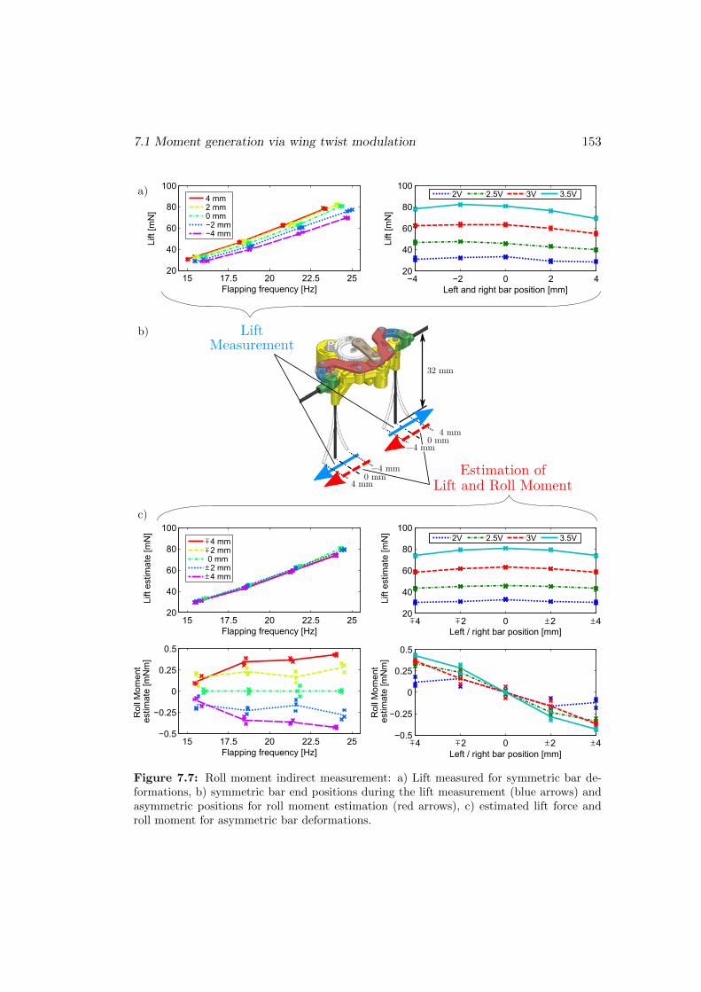
7.1 Moment generation via wing twist modulation 153
Left and right bar position [mm]
−4 −2 0 2 420
40
60
80
100
Lift
[mN
]
2V 2.5V 3V 3.5V
20
40
60
80
100
−0.5
−0.25
0
0.25
0.5
15 17.5 20 22.5 2520
40
60
80
100
Flapping frequency [Hz]
15 17.5 20 22.5 2520
40
60
80
100
Flapping frequency [Hz]
15 17.5 20 22.5 25−0.5
−0.25
0
0.25
0.5
Flapping frequency [Hz]
Roll
Mom
ent
Estimation ofLift and Roll Moment
4 2 0 2 4±∓ ∓ ±
4 2 0 2 4±∓ ∓ ±
4 mm2 mm0 mm−2 mm−4 mm
2V 2.5V 3V 3.5V4 mm2 mm
0 mm2 mm4 mm
∓
±
±
∓
LiftMeasurement
32 mm
0 mm−4 mm
4 mm
0 mm4 mm
−4 mm
estim
ate
[m
Nm
]Lift
estim
ate
[m
N]
Roll
Mom
ent
estim
ate
[m
Nm
]Lift
estim
ate
[m
N]
Lift
[mN
]
Left / right bar position [mm]
Left / right bar position [mm]
a)
b)
c)
Figure 7.7: Roll moment indirect measurement: a) Lift measured for symmetric bar de-formations, b) symmetric bar end positions during the lift measurement (blue arrows) andasymmetric positions for roll moment estimation (red arrows), c) estimated lift force androll moment for asymmetric bar deformations.

154 7 Control mechanism
7.1.3 SMA actuated control mechanism
One of the concepts considered for active displacement of the bar ends is using ShapeMemory Alloys (SMA) wires as actuators. The material uses a shape memory ef-fect: when heated above certain temperature the crystal structure changes and, ifthe material is under stress, we observe contraction of the wire. After cooling theoriginal shape is restored (Lagoudas, 2008).
The use, advantages and limitations of SMAs were thoroughly reviewed by Mohd Janiet al. (2014). We chose this actuator because it is very lightweight and provides di-rectly a displacement. It can be heated simply by Joule effect. But it also has somelimitations that need to be considered in the design: the maximal stroke is onlyabout 5% of the wire length. The necessary (passive) cooling reduces significantlythe bandwidth. Moreover, the material has a hysteretic behaviour due to phasetransformation: the heating follows different characteristics than the cooling. It canalso suffer from fatigue, so operation at smaller strains (under 3.5%) and limitedstresses (under 160MPa) is recommended (SAES Getters, 2009).
The use of flexible bars instead of joints not only reduces the control mechanism com-plexity, but the bar deformation also creates the stress necessary for SMA properfunction. The small stroke achievable with an SMA wire can be overcome by thekinematics. The SMA wire is attached between two supports; the distance betweenthese is just slightly shorter than the length of the SMA wire itself. Thus, a smallcontraction of the wire results in a relatively large displacement in the normal di-rection (Figure 7.8 left). The downside of this approach is that the maximal forceis also reduced.
COLD
HOT Front wire on(nose-down
pitch)
Rear wire on(nose-uppitch)
Both wires on(roll)
Both wires off(hover)
SMA wire
Figure 7.8: SMA driven control mechanism: kinematics for larger stroke (left), bottomview of the mechanism model (middle) with corresponding stress distribution for the frontwire (right). The two supports are on top of each other in the bottom view.
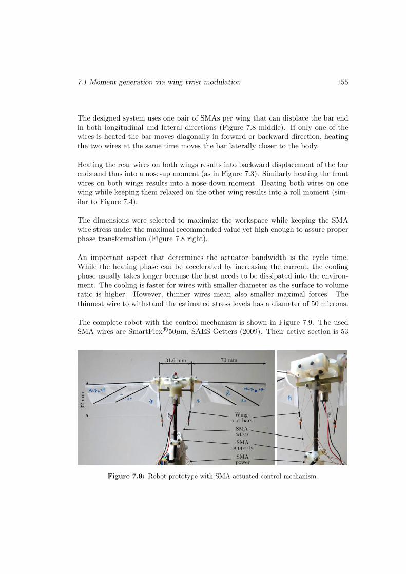
7.1 Moment generation via wing twist modulation 155
The designed system uses one pair of SMAs per wing that can displace the bar endin both longitudinal and lateral directions (Figure 7.8 middle). If only one of thewires is heated the bar moves diagonally in forward or backward direction, heatingthe two wires at the same time moves the bar laterally closer to the body.
Heating the rear wires on both wings results into backward displacement of the barends and thus into a nose-up moment (as in Figure 7.3). Similarly heating the frontwires on both wings results into a nose-down moment. Heating both wires on onewing while keeping them relaxed on the other wing results into a roll moment (sim-ilar to Figure 7.4).
The dimensions were selected to maximize the workspace while keeping the SMAwire stress under the maximal recommended value yet high enough to assure properphase transformation (Figure 7.8 right).
An important aspect that determines the actuator bandwidth is the cycle time.While the heating phase can be accelerated by increasing the current, the coolingphase usually takes longer because the heat needs to be dissipated into the environ-ment. The cooling is faster for wires with smaller diameter as the surface to volumeratio is higher. However, thinner wires mean also smaller maximal forces. Thethinnest wire to withstand the estimated stress levels has a diameter of 50 microns.
The complete robot with the control mechanism is shown in Figure 7.9. The usedSMA wires are SmartFlex R©50µm, SAES Getters (2009). Their active section is 53
31.6 mm 70 mm
32 m
m
SMAwires
SMAsupports
Wingroot bars
SMApower
Figure 7.9: Robot prototype with SMA actuated control mechanism.

156 7 Control mechanism
mm long, the distance between the supports is 47 mm. The system to attach theSMA wires consists of two washers under the head of a bolt. The SMA wire goesaround the bolt and is pressed between the washers. The power is brought by an-other cable, pressed by the second washer to the support.
7.1.4 SMA driven control mechanism performance
To determine the mechanism bandwidth the front and rear pair of wires were peri-odically heated and cooled in an alternating manner, i.e. the bars were alternatingbetween the positions for nose-down and nose-up pitch moment. The achieved dis-placement was measured from a long exposure camera image. The duty cycle was50 % and the frequency was being changed from 1 Hz to 5Hz. The current wasconstant during the heating phase, a value of 110 mA was identified as optimal (nooverheating). The airflow from the wings accelerated the cooling process. The re-sults presented in Figure 7.10 were measured at a moderate flapping frequency ofabout 16 Hz. The maximal displacement of 2.9 mm at 1 Hz decreases significantly asthe command becomes faster. According to the results from the previous section themaximal displacement would generate a pitch moment of approximately ± 0.2 mNm.
1 2 3 4 50
0.5
1
1.5
2
2.5
3
Driving frequency [Hz]
∆ [m
m]
Figure 7.10: Long exposure images of root bar displacement by the SMA actuators drivenat various frequencies (top) and processed results (bottom).

7.1 Moment generation via wing twist modulation 157
15 17.5 20 22.50
20
40
60
Flapping frequency [Hz]
Lift
[mN
]
Hover Nose down Nose up
15 17.5 20 22.5
0.15
0.075
0
0.075
0.15
Flapping frequency [Hz]
Pitch
mo
me
nt [m
Nm
]
Nose down Hover Nose up0
20
40
60
Lift
[mN
]
Nose down Hover Nose up
0.15
0.075
0
0.075
0.15
Bar position [ ]
~2V ~2.5V ~3V
Bar position [ ]
Pitch
mo
me
nt
[mN
m]
Figure 7.11: Lift and moment measurement results - SMA actuated bar displacement.
A direct pitch moment measurement was carried out in three (steady) positions ac-cording to Figure 7.8 (right): 1) in the hover position with all the wires relaxed,2) in the nose-up moment position with the rear pair of wires heated and 3) in thenose-down moment position with the front pair of wires heated. The measurementwas repeated five times in each position. The results are plotted in Figure 7.11;individual measurements are displayed as crosses and the lines represent the averagevalues. The lift in hover position is slightly lower when compared to both nose-upand nose-down positions. This is in accordance with our expectations, because togenerate a moment the wing root bar moves also in lateral direction which stretchesthe wing membrane and results in a lift increase.
The maximum generated pitch moment is approximately -0.11 mNm (nose-up) and0.06 mNm (nose-down), which is already at the limit of the resolution of the forcebalance. The moments are lower than ± 0.2 mNm estimated from the results inprevious section, probably due to smaller bar displacements at higher flapping fre-quencies that involve higher stress and higher cooling rates. However, direct com-parison is not completely correct as the wing design in the SMA actuated prototypehad to be modified to compensate for the wing root bar deformation, that needsto be present even in hover position to create pre-stress. The asymmetry betweennose-up and nose-down moments might come from imperfections of the hand builtprototype (slight misalignment of the SMA supports, small variations of the SMA

158 7 Control mechanism
wires lengths, ...). The indirect measurement of the roll moment estimated evenlower moment values, which were already at the level of variation among individualmeasurements, because the SMA wires didn’t provide enough displacement.
7.1.5 Conclusion on wing twist modulation
The presented concept, combining the wing twist modulation with flexible wingroot bars, proved to be a feasible solution for generating the control moments. Theexperiments showed that a (manual) bar displacement of ±4 mm can generate apitch moment of ±0.5 mNm and roll moment of ±0.4 mNm, which is about 4 timesand 8 times the necessary value, respectively, predicted by the flight simulation inSection 5.3. The maximal generated lift produced during the experiments (about85 mN) was close to the maximal performance of the flapping mechanism at thetime of the experiment. Because the control mechanism only acts on the root barends, it is completely independent on the flapping mechanism. The newest flappingmechanism version produces almost twice as much lift and so a similar increase inthe pitch moment can be expected.
The actively controlled mechanism driven by SMA wires was attractive due to itslow weight and relatively low complexity. However, several weak points of this so-lution were identified. Most importantly, the bandwidth as well as the achievablestroke (and thus the moments) were too low. Apart from that, it was cumbersometo adjust the initial stress in the SMA wires and many wire failures were experienceddue to stress concentration in the attachment points. Thus, the full potential of theconcept should be exploited by an alternative solution using actuators with largerstroke and higher bandwidth, such as micro-servomotors.
7.2 Moment generation via amplitude and offsetmodulation
The second concept generates the control moments by modulating the flapping am-plitude and offset (mean wing position) according to Figure 7.12. This strategywas also used in the simulation presented in Chapter 5. Compared to wing twistmodulation this strategy is more straight forward and works with any wing design.However, it requires a modification of the flapping mechanism. The roll moment isproduced by increasing the amplitude of one wing and decreasing the amplitude ofthe other wing, which introduces a lift imbalance between the two wings. Movingthe mean wing position of both wings forward or backward results into a nose-up or

7.2 Moment generation via amplitude and offset modulation 159
Figure 7.12: Moment generation via flapping amplitude and offset modulation.
nose-down pitch moment as the mean lift force origin moves forward or backwardfrom the COG, respectively. Yaw moment generation is not so evident, but themathematical model in Section 5.2 predicts that the necessary drag imbalance canalso be introduced by changing the mean wing position asymmetrically, see equation(5.13).
7.2.1 Amplitude and offset modulation
During the flapping mechanism optimization process it has been found that boththe flapping amplitude and the offset can be controlled by displacing the mechanismjoints A and B, highlighted in Figure 7.13 a). The map in Figure 7.13 b) showsthe relation between the position of the joint and the wing amplitude Φ and offsetφ0. The blue lines connect positions with constant offset and the red lines con-nect positions with constant amplitude. Thus, moving the joint along a blue linewill modify the amplitude, but the offset will remain constant. Similarly a displace-ment along a red line will only affect the offset while keeping the amplitude constant.
It can be noticed that the two sets of curves cross each other at high angles (above70) meaning the two parameters can be controlled independently. Moreover, thelines of constant offset are almost straight and nearly parallel; the curves of constant
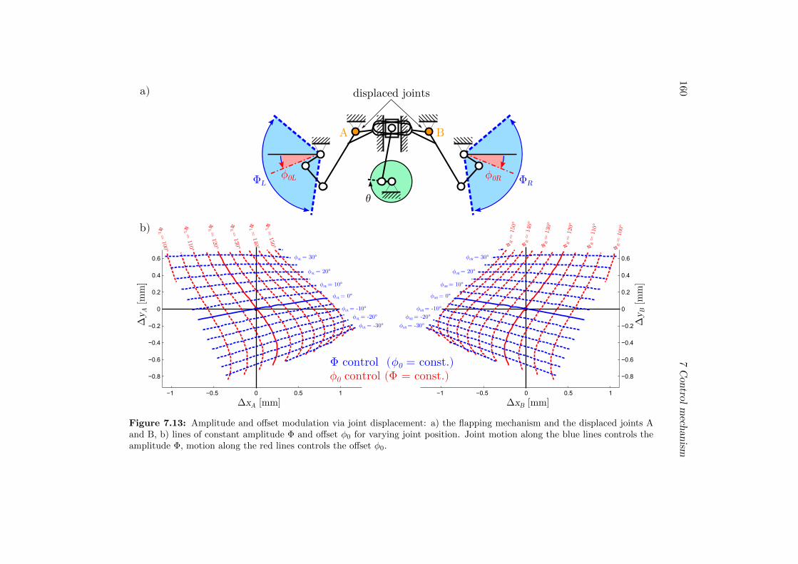
1607
Con
trolm
echan
ism
−1 −0.5 0 0.5 1
−0.8
−0.6
−0.4
−0.2
0
0.2
0.4
0.6
ΦL =
120°
ΦL =
110°
ΦL =
130°
ΦL =
140°
ΦL =
150°
ΦL =
100°
ϕ0L
= 0°
ϕ0L
= 10°
ϕ0L
= 20°
ϕ0L
= 30°
ϕ0L
= -10°
ϕ0L
= -20°
ϕ0L
= -30°
ΔxA [mm]
Δy
A [m
m]
−0.8
−0.6
−0.4
−0.2
0
0.2
0.4
0.6
ΦR
=
120°
ΦR
=
110°
ΦR
=
130°
ΦR
=
140°
ΦR
=
150°
ΦR
=
100°
ϕ0R
= 0°
ϕ0R
= 10°
ϕ0R
= 20°
ϕ0R
= 30°
ϕ0R
= -10°
ϕ0R
= -20°
ϕ0R
= -30°
ΔxB [mm]
Δy
B [m
m]
θ
ΦL
ϕ0L ΦR
ϕ0R
−1 −0.5 0 0.5 1
A B
Φ control (ϕ0 = const.)
ϕ0 control (Φ = const.)
a)
b)
displaced joints
Figure 7.13: Amplitude and offset modulation via joint displacement: a) the flapping mechanism and the displaced joints Aand B, b) lines of constant amplitude Φ and offset φ0 for varying joint position. Joint motion along the blue lines controls theamplitude Φ, motion along the red lines controls the offset φ0.

7.2
Mom
ent
genera
tionvia
am
plitu
de
and
offset
mod
ulation
161
−1 −0.5 0 0.5 1
−0.8
−0.6
−0.4
−0.2
0
0.2
0.4
0.6
ΔxA [mm]
Δy
A [m
m]
η = constεL = const
Δη =
0°
Δη =
-4°
Δη =
-8°
Δη =
4°
Δη =
8°
ΔεL = 0°
ΔεL = 4°
ΔεL = 8°
ΔεL = -4°
ΔεL = -8°
−0.8
−0.6
−0.4
−0.2
0
0.2
0.4
0.6
ΔxB [mm]
Δy
B [m
m]
η = constεR = const
Δη
= 0
°
Δη
= 4
°
Δη
= 8
°
Δη
= -4°
Δη
= -8°
ΔεR = 0°
ΔεR = 4°
ΔεR = 8°
ΔεR = -4°
ΔεR = -8°
η εL εRη
ROLL CONTROL
(ΔΦL = -ΔΦR)
PITCH CONTROL (εL = εR)
A Bϕ0L ϕ0R
ΦRΦL
YAW CONTROL (εL = -εR)a)
b)
−1 −0.5 0 0.5 1
Figure 7.14: Amplitude and offset modulation via joint displacement: a) the control mechanism with 3DOF (εL, εR, η) definingthe position of joints A and B by an intersection of two mobile slots, b) lines of constant commands ε and η approximatingwell the lines of constant amplitude Φ and offset φ0 in Figure 7.13 b). Joint motion along the magenta lines controls the rollmoment, motion along the green lines controls the pitch (∆εL = ∆εR) or yaw (∆εL = −∆εR) moments.

162 7 Control mechanism
amplitude are also equally spaced and can be approximated by straight lines aroundthe nominal position. This allows to design a joint displacement mechanism withtwo DOFs where the control is decoupled - one DOF controls directly the amplitudeand the other controls the offset.
7.2.2 Control mechanism prototype
The scheme of the proposed mechanism for joint displacement is shown in Figure7.14 a). Each joint is displaced by two arms with slots that rotate with respect to theframe by angles ε and η, respectively. The joint position is defined by an intersectionof the two slots. The arm hinges are located on the lines of nominal amplitude andof the nominal offset, respectively. If one of the arms is blocked and the other oneis moving, the joint moves along a line defined by the slot of the blocked arm. Ifthe hinges are placed far enough from the nominal position of the displaced joint(∆x = 0, ∆y = 0), these lines appear nearly parallel in the region of interest andthe joint paths approximate well the theoretical curves of constant amplitude andoffset, see Figure 7.14 b).
The control of left and right wing offset needs to be independent, operated by sep-arate actuators: a symmetric offset change (∆εL = ∆εR) produces pitch momentwhile an asymmetric change (∆εL = −∆εR) produces yaw moment. However, theamplitude can be controlled by a single actuator (η) since only asymmetric ampli-tude changes are needed for roll. This can be achieved by a parallelogram linkingthe two arms responsible for amplitude control as is shown in Figure 7.14 a).
The final mechanical solution of the joint displacement mechanism is shown in Figure7.15. The rivets of the joints to be displaced are fixed from the top to ”anchors” thatare free to slide in the horizontal plane of the frame. The displacement is limitedto the zone considered in Figure 7.14 b) by the shape of the frame cut-out. All theparts were 3D printed, a photograph of an assembled prototype is shown in Figure7.16. The mechanism is actuated by three micro servos (HobbyKing 5330) with aweight of 2.0 g each. The total weight of the controlled prototype including theservos (6.0 g) and the propulsion motor (5.2 g) is 21.4 g.
7.2.3 Wing kinematics
A high speed camera (Photron FASTCAM SA3) was used to study the changes in thewing kinematics of the control prototype. The wing motion was recorded at 500 fpsunder different control commands and the sweep angle φ was tracked in the record-ings (see Figure 6.9 in the previous chapter for its definition). As already mentionedin Section 6.2.1 the observed amplitudes were much larger than the design value of

7.2 Moment generation via amplitude and offset modulation 163
Roll servo arm
Topview
Sectionview
Bottomview
Explodedview
Displaced joints
Right offsetservo arm
Left offsetservo arm
Roll controlparallelogram
Controlservos
Controlmechanism
Flappingmechanism
PropulsionDC motor
"Anchor" sliding freely inside the frame
Figure 7.15: CAD model of the control prototype. Details of the flapping mechanism withthe joint displacement system (left) and an exploded view of the whole prototype (right).
Figure 7.16: The assembled prototype with pitch, roll and yaw control via joint displace-ment.
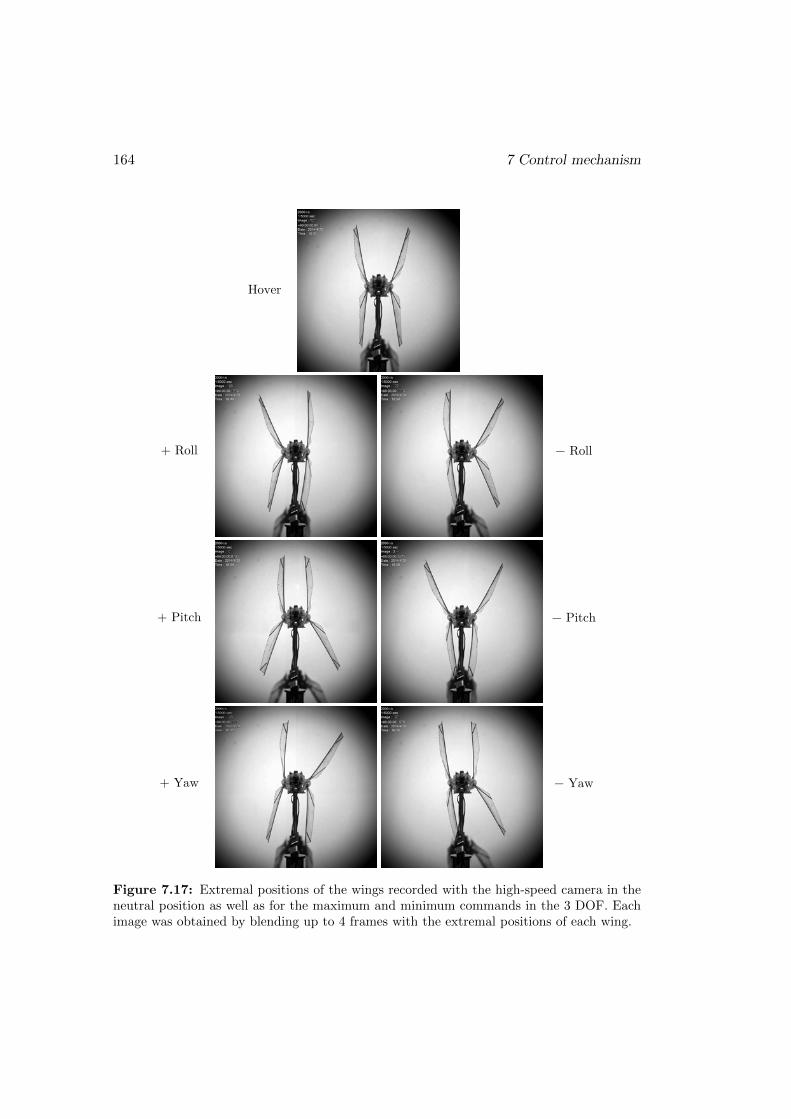
164 7 Control mechanism
+ Roll
+ Pitch
+ Yaw
Hover
− Roll
− Pitch
− Yaw
Figure 7.17: Extremal positions of the wings recorded with the high-speed camera in theneutral position as well as for the maximum and minimum commands in the 3 DOF. Eachimage was obtained by blending up to 4 frames with the extremal positions of each wing.

7.2 Moment generation via amplitude and offset modulation 165
120 due to the wing bars compliance and partly also due to the mechanism back-lash. Unless mentioned otherwise, the tests were carried out at a moderate flappingfrequency of 15Hz in order to have consistent results along all the tests. For higherfrequencies the prototype performance can slightly deteriorate over time due to wear.
The wing extremal positions under maximal and minimal commands of pitch, rolland yaw are displayed in Figure 7.17. The mechanism succeeds to modify the flap-ping amplitude and offset in the desired manner. The roll and pitch command willbe studied in more detail in the following text. The performance in yaw is the sameas in pitch, only the left and right wing offset commands have opposite signs.
Figure 7.18 shows the results of amplitude difference control. The servos controllingthe wing offset were kept in their nominal position and the roll control servo wascommanded from the minimal to the maximal position with a step of 10% of the fullrange. The left and right wing amplitudes, ΦL and ΦR, are approximately equal forzero servo position. As intended, their difference ∆Φ = ΦR−ΦL increases/decreasesapproximately linearly as the servo moves towards the positive/negative limit, wherethe difference is +52 and −44, respectively. Thus, a good control authority of theroll moment is achieved. The wing offset remains relatively close to zero and theaverage amplitude Φ = (ΦR + ΦL)/2 stays approximately constant (around 155)in the central part of the servo range. There exist some imperfections, in particularclose to the limits, but these should be compensated by the flight controller feedbackin future.
−1 −0.5 0 0.5 1120
140
160
180
Fla
ppin
g a
mplit
ude [
°]
−1 −0.5 0 0.5 1−20
−10
0
10
20
Servo position [−]
Win
g o
ffset
[°]
Average Right wing Left wing
Figure 7.18: Amplitude control with the roll servo.
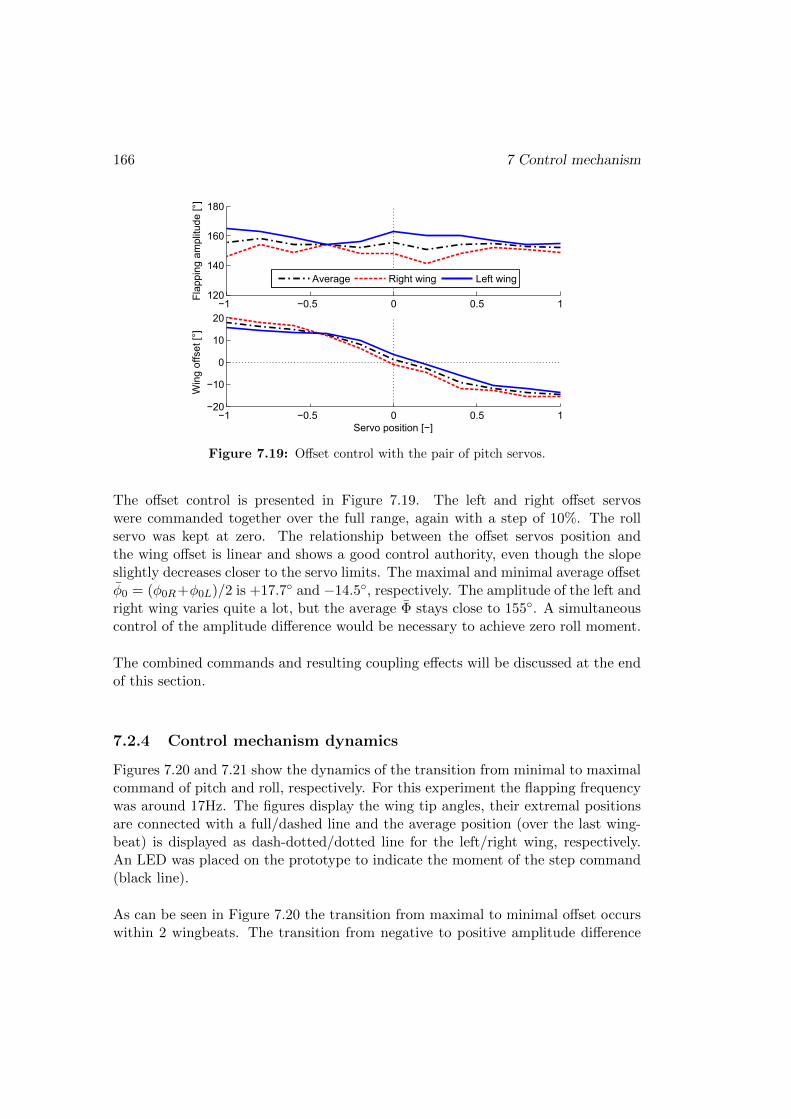
166 7 Control mechanism
−1 −0.5 0 0.5 1120
140
160
180F
lappin
g a
mplit
ude [
°]
−1 −0.5 0 0.5 1−20
−10
0
10
20
Servo position [−]
Win
g o
ffset
[°]
Average Right wing Left wing
Figure 7.19: Offset control with the pair of pitch servos.
The offset control is presented in Figure 7.19. The left and right offset servoswere commanded together over the full range, again with a step of 10%. The rollservo was kept at zero. The relationship between the offset servos position andthe wing offset is linear and shows a good control authority, even though the slopeslightly decreases closer to the servo limits. The maximal and minimal average offsetφ0 = (φ0R+φ0L)/2 is +17.7 and −14.5, respectively. The amplitude of the left andright wing varies quite a lot, but the average Φ stays close to 155. A simultaneouscontrol of the amplitude difference would be necessary to achieve zero roll moment.
The combined commands and resulting coupling effects will be discussed at the endof this section.
7.2.4 Control mechanism dynamics
Figures 7.20 and 7.21 show the dynamics of the transition from minimal to maximalcommand of pitch and roll, respectively. For this experiment the flapping frequencywas around 17Hz. The figures display the wing tip angles, their extremal positionsare connected with a full/dashed line and the average position (over the last wing-beat) is displayed as dash-dotted/dotted line for the left/right wing, respectively.An LED was placed on the prototype to indicate the moment of the step command(black line).
As can be seen in Figure 7.20 the transition from maximal to minimal offset occurswithin 2 wingbeats. The transition from negative to positive amplitude difference
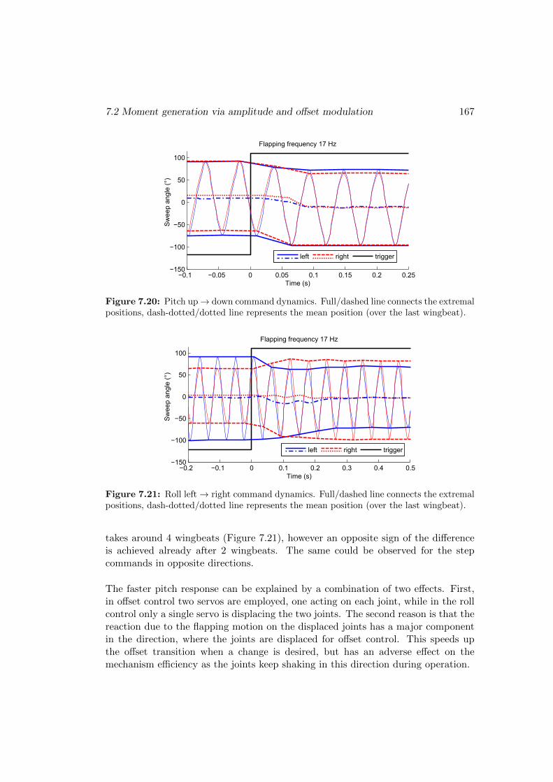
7.2 Moment generation via amplitude and offset modulation 167
−0.1 −0.05 0 0.05 0.1 0.15 0.2 0.25−150
−100
−50
0
50
100
Time (s)
Sw
eep a
ngle
(°)
Flapping frequency 17 Hz
left right trigger
Figure 7.20: Pitch up→ down command dynamics. Full/dashed line connects the extremalpositions, dash-dotted/dotted line represents the mean position (over the last wingbeat).
−0.2 −0.1 0 0.1 0.2 0.3 0.4 0.5−150
−100
−50
0
50
100
Time (s)
Sw
eep a
ngle
(°)
Flapping frequency 17 Hz
left right trigger
Figure 7.21: Roll left→ right command dynamics. Full/dashed line connects the extremalpositions, dash-dotted/dotted line represents the mean position (over the last wingbeat).
takes around 4 wingbeats (Figure 7.21), however an opposite sign of the differenceis achieved already after 2 wingbeats. The same could be observed for the stepcommands in opposite directions.
The faster pitch response can be explained by a combination of two effects. First,in offset control two servos are employed, one acting on each joint, while in the rollcontrol only a single servo is displacing the two joints. The second reason is that thereaction due to the flapping motion on the displaced joints has a major componentin the direction, where the joints are displaced for offset control. This speeds upthe offset transition when a change is desired, but has an adverse effect on themechanism efficiency as the joints keep shaking in this direction during operation.

168 7 Control mechanism
7.2.5 Pitch moment and lift generation
Apart from the wing kinematics measurements, the generated lift and pitch momentwas measured directly on the force balance presented in Section 6.2.2. Figure 7.22shows the measured pitch moment, lift, frequency and motor current for the fullrange of the pitch servos. The motor voltage was kept at 4.2V, which gives a flap-ping frequency of approximately 15Hz for the nominal servo position. The measuredpitch moment ranged from -0.5 mNm to 0.8 mNm. The lift force and the flappingfrequency increase and the current decreases when the servos approach the servolimits. This is caused by the shaking of the displaced joints due to flapping (alreadymentioned earlier) that happens particularly for the central servo positions. Thejoints get a better fix in the limit positions, where the servo pushes the displacedjoints against a wall of the frame, and thus the efficiency increases. The lift variesbetween 53 and 59 mN and the frequency between 14.9 and 16.2 Hz.
−1 −0.5 0 0.5 150
52
54
56
58
60
62
Pitch servo [−]
Lift
[mN
]
−1 −0.5 0 0.5 1
−0.5
0
0.5
1
Pitch servo [−]
−1 −0.5 0 0.5 10.22
0.24
0.26
0.28
0.3
0.32
Pitch servo [−]
Curr
ent
[A]
−1 −0.5 0 0.5 114.5
15
15.5
16
16.5
Pitch servo [−]
Fre
quency [
Hz]
Figure 7.22: Lift, pitch moment, motor current and flapping frequency against pitchservos position. Measurement done at 4.2 V leading to 15 Hz at the nominal position.Individual measurements are displayed as crosses, the solid line represents an average offour measurements.

7.2 Moment generation via amplitude and offset modulation 169
Figure 7.23 combines the moment measurement with the wing kinematics measure-ment from the previous section. The relationship is approximately linear with aslope of 0.04 mNm per degree of the offset φ0. The non-zero moment produced atzero offset can be explained by a combination of asymmetric wing design (stiffenersglued only on one side of the membrane), different velocity profiles in upstroke anddownstroke and by an imperfect alignment of the prototype on the balance. Never-theless, a compensating moment can be easily introduced by an offset of the COGfrom the shoulders in the longitudinal direction.
−20 −10 0 10 20−1
−0.5
0
0.5
1
Offset [°]
Figure 7.23: Pitch moment against wing offset φ0.
Figure 7.24 shows the pitch moment, lift, frequency and motor current for motorvoltages up to 6V. The three curves represent the measurements for servo positions-1, 0 and 1, respectively, related to the full range. The behaviour corresponds to theone observed at 15Hz. At the highest tested voltage the mechanism produces pitchmoments from -0.7 mNm to 1.1 mNm while the lift ranges between 90 and 100 mN.
The lift vs frequency characteristic is close to the one of the uncontrolled prototype(with fixed joints), see Figure 7.25, with only small differences caused by a variationof the flapping amplitude. However, the electrical power of the controlled versionis almost twice as high due to losses in the shaking joints. Thus, the mechanicaldesign of the joint displacement mechanism needs to be improved in order to get abetter fix of the joints and, subsequently, a better efficiency.

170 7 Control mechanism
3 4 5 60
25
50
75
100
Motor voltage [V]
Lift
[mN
]
3 4 5 6
Figure 7.24: Lift, pitch moment, motor current and flapping frequency measured forincreasing motor voltage. Black lines represent the zero pitch servos position, red and bluelines represent the minimal and maximal pitch command. The crosses represent individualmeasurements.
10 12 14 16 18 202
4
6
8
10
12
Frequency [Hz]
Lift
[g]
0 1 2 32
4
6
8
10
12
Electrical power [W]
Lift
[g]
Joints fixed
Pitch 1
Pitch 0
Pitch −1
Figure 7.25: Pitch moment against wing offset.

7.2 Moment generation via amplitude and offset modulation 171
7.2.6 Combined commands
Finally, combined pitch and roll commands were tested to identify the amount ofcross-coupling. Again all the measurements were carried out at a constant motorvoltage (4.2V) giving a flapping frequency of around 15Hz at the nominal positionof the servos. The measurements were taken at servo positions -0.8, -0.4, 0, 0.4 and0.8 of the full range for both pitch and roll servos. Thus, 25 measurements weretaken in total.
Figure 7.26 shows the amplitude and offset maps of the left and the right wing fromthe high speed recordings. The camera images combining the extremal wing posi-tions for maximal commands (corners of the maps) are shown in Figure 7.27. Wecan see that while a small cross-coupling always exists, the roll servo has a domi-nant effect on the amplitude and the pitch servo has a dominant effect on the offset.Moreover, the relation between the amplitude/offset and roll/pitch servo positions
a) b)
c) d)
Figure 7.26: Experimental results: Kinematics for combined pitch and roll servo com-mands. a) Left amplitude, b) right amplitude, c) left offset, d) right offset.

172 7 Control mechanism
+ Roll − Roll
− Pitch
+ Pitch + Pitch
− Roll+ Roll
− Pitch
Figure 7.27: Extremal positions of the wings recorded with the high-speed camera for thecombined commands in pitch and roll. Each image was obtained by blending up to 4 frameswith the extremal positions of each wing.
stays always monotonic. Thus, a feedback controller should be able to compensatethe coupling effects and the small differences between the left and right wing be-haviour, caused by the mechanism imperfections.
The same experiment was repeated with the force balance, the results are shown inFigure 7.28. The maps show the pitch moment and lift force for the selected servoinput combinations. The lift map keeps a valley-like shape in the pitch servo direc-tion, similar to what was observed for the pure pitch command and what can beexplained by an improper joint fixation in the central pitch servo positions. There isalso a smaller increase of lift in the positive roll direction, which most likely comesfrom the imperfections of the prototype. The minimum and maximum lift is 48 and59 mN, respectively. The lift force variation is related to the square of frequencytimes amplitude displayed in Figure 7.29 c), in accordance with equation (6.8).
The pitch moment depends mostly on pitch servo positions, while there are onlyminor differences when the roll servo position changes. Thus, the minimal and max-imal pitch moment values stay at the same levels as for the pure pitch command,-0.4 mNm and 0.8 mNm respectively. The pitch moment corresponds closely to themean offset shown in Figure 7.29 a).

7.2 Moment generation via amplitude and offset modulation 173
a) b)
Figure 7.28: Experimental results: Force balance measurements for combined pitch androll servo commands. a) Lift, b) pitch moment. Lift is tied to the square of mean amplitudetimes frequency in Figure 7.29 a), pitch moment to the mean offset in Figure 7.29 b).
a) b)
c)
Figure 7.29: Experimental results: Kinematics for combined pitch and roll servo com-mands. a) Square of mean amplitude times frequency, b) mean wing offset, c) flappingamplitude difference.

174 7 Control mechanism
The roll moment could not be measured directly, but it should correspond to theamplitude difference shown in Figure 7.29 c).
7.2.7 Conclusion on amplitude and offset modulation
The second presented control mechanism generates the necessary control momentsby modulating the flapping wing amplitude and offset. The wing kinematics mod-ifications are achieved by displacing the joints of the flapping linkage mechanism.It was demonstrated experimentally that sufficient offset (±15) and amplitude dif-ferences (above ±40) for pitch and roll control can be introduced by very smalldisplacements of the linkage joints (below ±1mm) in two directions. The transi-tions between maximum and minimum command takes less than two wingbeats inpitch and about four wingbeats in roll. A very low level of cross-coupling existsfor combined commands. The prototype can produce pitch moments between -0.7mNm and 1.1 mNm (at least 6 times the moment predicted by the flight simulationin Section 5.3) while flapping at frequencies around 18Hz and producing a lift ofat least 90mN. The roll moment could not be measured, but should be more thansufficient as the measured amplitude differences are 40 times higher than those pre-dicted by flight simulation.
While the control mechanism succeeds in modifying the wing kinematics and, subse-quently, in the moment generation with sufficient dynamics, the prototype efficiencydrops significantly compared to the uncontrolled prototype. The drawback of theproposed solution is that the displaced joints need to hold rather large and oscillatingreaction forces due to flapping. This causes the joints to shake, which reduces signif-icantly the mechanism performance and at higher frequencies also its lifespan. Themotor draws up to twice the electrical power compared to an uncontrolled prototypewith fixed joints. Thus, an alternative mechanical solution, which would reduce theeffect of the oscillating reaction forces on the servos displacing the joints, should befound.
7.3 Discussion and conclusions
Two control mechanisms generating moments around the three body axis (roll, pitch,yaw) were developed and tested. The first solution, based on wing twist modulation,is inspired by the control mechanism of the Nano Hummingbird (Keennon et al.,2012). The second, original solution generates the moments by flapping amplitudeand offset modulation through displacements of the flapping mechanism linkagejoints. Both control mechanisms succeeded in generating moments that were several

7.3 Discussion and conclusions 175
times higher than the moments needed in the flight simulation in Chapter 5. Nev-ertheless, the experiments revealed that each of the mechanisms has several strongpoints, but also some weaknesses that require further development.
The advantage of the wing twist modulation mechanism is that it is fully inde-pendent on the flapping mechanism. It acts at the wing root bar ends, where thereaction forces, that it needs to hold, are relatively small (compared to the secondsolution). This is advantageous as it permits the use of smaller and lighter actuators.Moreover, the use of flexible root bars instead of universal joints greatly reduces themechanism complexity. On the other hand, the wing twist modulation concept re-quires a specific wing design, whose lift force varies approximately linearly with theroot bar deformation. This requires that the wing at the nominal bar position isoperated below its maximal lift.
The second mechanism modulating the flapping amplitude and offset works withany wing design. It is an integral part of the flapping mechanism as it displacesone of the linkage joints. This can be considered as beneficial as the whole designis compact and the actuators can be placed close to the flapping mechanism part.On the other hand, any design change of the flapping mechanism requires also aredesign of the joint displacement system. Another drawback of this solution is thatthe system needs to hold the reaction forces from the displaced joints, which are inparticular high in the pitch control direction. This made the joints shake during theoperation and resulted into efficiency degradation.
A remaining challenge for both solutions are the actuators. The most fitting actu-ators for this application on the market, the smallest available micro servos, havean acceptable power, but remain still relatively large and heavy. While they showedsufficient dynamics in the joint displacement system, they were unable to fix thejoints completely. Nevertheless, a modified mechanical solution might succeed inreducing the joint shaking.
As an alternative, a shape memory alloy actuator was used in the wing twist mod-ulation system. This actuator is very light and provides satisfactory stroke in staticexperiments, however its performance decreases significantly under dynamic testsand thus it is not a good candidate for the control actuator.
To conclude, both presented control systems succeed in moment generation, butrequire further development and testing, focused mostly on efficiency improvementsand weight reduction. In future, a combination of both systems might also beconsidered in order to solve potential cross-coupling of the three generated controlmoments.

176 References
7.4 References
M. Karasek, Y. Nan, I. Romanescu, and A. Preumont. Pitch moment generationand measurement in a robotic hummingbird. International Journal of Micro AirVehicles, 5(4):299–310, 2013. doi:10.1260/1756-8293.5.4.299.
M. Karasek, A. Hua, Y. Nan, M. Lalami, and A. Preumont. Pitch and roll controlmechanism for a hovering flapping wing MAV. In International Micro Air VehicleConference and Flight Competition (IMAV2014), Delft, The Netherlands, August12-15, pages 118–125, 2014.
M. T. Keennon, K. R. Klingebiel, H. Won, and A. Andriukov. Development ofthe nano hummingbird: A tailless flapping wing micro air vehicle. AIAA paper2012-0588, pages 1–24, 2012.
D. C. Lagoudas. Shape Memory Alloys: Modeling and Engineering Applications.Springer, 2008. doi:10.1007/978-0-387-47685-8.
K. Y. Ma, P. Chirarattananon, S. B. Fuller, and R. J. Wood. Controlledflight of a biologically inspired, insect-scale robot. Science, 340:603–607, 2013.doi:10.1126/science.1231806.
J. Mohd Jani, M. Leary, A. Subic, and M. A. Gibson. A review of shape memoryalloy research, applications and opportunities. Materials & Design, 56:1078–1113,2014. doi:10.1016/j.matdes.2013.11.084.
SAES Getters. Smartflex wire & springs. http://www.saesgetters.com/sites/
default/files/SmartFlex%20Wire%20%26%20Spring%20datasheets_1.pdf,2009. Accessed: 18/08/2014.
T. Q. Truong, V. H. Phan, S. P. Sane, and H. C. Park. Pitching moment generationin an insect-mimicking flapping-wing system. Journal of Bionic Engineering, 11(1):36–51, 2014.
Chapter 8
Summary and conclusions
This work dealt with development of a hummingbird-sized tail-less flapping wingmicro air vehicle capable of hovering. More specifically, the aim of this thesis was todevelop a control mechanism that generates the moments controlling the flight byvarying the wing motion of each wing independently.
First, the problem was studied theoretically. In Chapter 3, a mathematical modelwas developed combining quasi-steady aerodynamics with rigid body dynamics. Themodel was linearised and further reduced. It has been shown that the model givescomparable results to CFD data from the literature. In Chapter 4, stability of thedesigned MAV was studied showing, in accordance with other studies, that hoveringflapping flight is inherently unstable. It has been demonstrated that stability canbe achieved with an angular rate feedback, which is most likely used by insects, aslong as the wings are placed sufficiently high above the centre of gravity. A flightcontroller with cascade structure has been designed in Chapter 5. Several ways ofgeneration of the necessary control moments by wing motion changes have beenidentified. A good control performance has been shown in simulation (using thefull, non-linear model) for an example of flapping amplitude and offset (mean wingposition) modulation.
A prototype of the robotic hummingbird was designed and tested in Chapter 6.The flapping mechanism has undergone a lot of development. Its dimensions wereoptimized for symmetric wing motion, which was confirmed by high speed camerameasurements. A force balance capable of measuring cycle averaged lift force andpitch moment was built to evaluate the prototype performance. The wing shapewas optimized experimentally for maximal lift. The latest prototype, with off-boardpower and no control, has a lift to mass ratio of nearly 1.3. A take off was demon-strated while the prototype was stabilized by a guide cable.
177

178 8 Summary and conclusions
Last but no least, two types of control mechanisms generating the necessary con-trol moments were designed in Chapter 7. The first solution generates the controlmoments by modulating the twist of the wings by flexing the wing root bars. Thesecond solution modulates the flapping amplitude and offset via displacements ofthe flapping mechanism joints in specific directions. Shape memory alloy actuatorswere employed to drive the first solution, however, the performance was not suffi-cient due to low bandwidth. Micro-servomotors were used for the second solutionand satisfactory response times were achieved. Prototypes of both solutions weretested on the force balance, both generating control moments several times largerthan the maximum control moments estimated in the flight control simulation.
8.1 Original aspects
The following parts of this work represent an original contribution:
• It has been shown, by comparing several aerodynamic models, that the com-plex non-linear dynamics of flapping flight, once cycle averaged, can be repre-sented by a reduced linear model, where the decoupled pitch and roll dynamicsare characterized by three poles each. The pole configuration depends on thewing position. If the wings are well above the centre of gravity, a simple an-gular rate feedback stabilizes the system.
• A new flapping mechanism with high amplitude consisting of two stages, aslider-crank and four-bar mechanisms, has been developed. The mechanismoutput has nearly symmetric velocity profile, which is ideal for hovering flightand a big advantage over single stage linkage mechanisms.
• A new control mechanism concept generating the necessary control momentsby amplitude and offset modulation via displacements of the flapping mecha-nism joints has been developed. The mechanism is tied to a specific flappingmechanism, but is fully independent of the wing design.
8.2 Future work
The developed robotic hummingbird demonstrated that it can generate sufficient liftto take-off or sufficient moments to stabilize itself in the air. However, the weight ofthe current design of the controlled prototype is too high (i) due to the used servo

8.3 Publications 179
actuators, (ii) because it was designed for bench tests, where robustness and long lifewere a priority and (iii) due to a relatively low strength to weight ratio of the photo-polymer material used in the 3D printing process. Thus, further development of therobot prototype is necessary, concentrating mainly on improving the lift productionand reducing the weight:
• The control mechanism should be redesigned to better fix the displaced joints.Currently, a significant amount of energy is lost because the joints shake whenflapping. A possible solution that uses cams to reduce the forces transferredto the servo actuators is already under development.
• Lightweight actuators with sufficient stroke and power need to be found ordeveloped. The shape memory alloy wires used in this study are light enough,but their response times are too slow and the stroke too short. The micro servo-motors have the necessary performance, but they are too heavy, representingalmost 30% of the total mass.
• The generated lift should be increased by optimizing further the wing designand by optimizing the gear-ratio for maximal efficiency of a specific motor-mechanism-wing combination.
• The robot structure mass needs to be reduced. It should be redesigned for pos-sible weight savings and a different manufacturing technology, using materialswith higher strength to mass ratio, should be considered.
Apart from the mechanical design, robot avionics, including a radio, an attitudesensor, a motor speed controller and a micro-controller needs to be integrated intoa sufficiently small and lightweight package, before a stable hovering flight can beachieved.
8.3 Publications
The work presented in this thesis has led to the following publications:
Journal papers
M. Karasek and A. Preumont. Flapping flight stability in hover: A comparison ofvarious aerodynamic models. International Journal of Micro Air Vehicles, 4(3):203–226, 2012. doi:10.1260/1756-8293.4.3.203.
M. Karasek and A. Preumont. Simulation of flight control of a hummingbird likerobot near hover. Acta Technica, 58(2):119–139, 2013.

180 8 Summary and conclusions
M. Karasek, Y. Nan, I. Romanescu, and A. Preumont. Pitch moment generationand measurement in a robotic hummingbird. International Journal of Micro AirVehicles, 5(4):299–310, 2013. doi:10.1260/1756-8293.5.4.299. The paper receivedthe ”Best Paper Award” at IMAV2013 conference.
Conference proceedings
M. Karasek and A. Preumont. Control of longitudinal flight of a robotic humming-bird model. In 5th ECCOMAS Thematic Conference on Smart Structures andMaterials SMART11, conference proceedings CD-ROM, Saarbrucken, Germany,July 6-8, 2011.
M. Karasek, A. Hua, Y. Nan, M. Lalami, and A. Preumont. Pitch and roll controlmechanism for a hovering flapping wing mav. In International Micro Air VehicleConference and Flight Competition (IMAV2014), Delft, The Netherlands, August12-15, pages 118–125, 2014.
Oral presentations and posters
M. Karasek and A. Preumont. Robotic hummingbird: Simulation model and longi-tudinal flight control (poster and oral presentation). International Workshop onBio-Inspired Robots, Nantes, France, April 6-8, 2011.
M. Karasek and A. Preumont. Flight simulation and control of a tailless flappingwing MAV near hover (poster). International Micro Air Vehicle Conference andFlight Competition (IMAV2012), Braunschweig, Germany, July 3-6, 2012.
M. Karasek and A. Preumont. Simulation of flight control of a hummingbird likerobot near hover (oral presentation). Engineering Mechanics 2012, Svratka, CzechRepublic, May 14-17, 2012.
M. Karasek, Y. Nan, I. Romanescu, and A. Preumont. Pitch moment generation andmeasurement in a robotic hummingbird (oral presentation). International MicroAir Vehicle Conference and Flight Competition (IMAV2013), Toulouse, France,September 17-20, 2013.
M. Karasek, I. Romanescu, and A. Preumont. Development of a robotic hum-mingbird (oral presentation). International Conference on Manufacturing Sys-tems (ICMS2013), Iasi, Romania, October 24-25, 2013.

General Bibliography
D. L. Altshuler and R. Dudley. Kinematics of hovering hummingbird flight alongsimulated and natural elevational gradients. Journal of Experimental Biology, 206:3139–3147, 2003. doi:10.1242/jeb.00540.
ATI Industrial Automation. Nano17 titanium. https://www.ati-ia.
com/products/ft/ft_models.aspx?id=Nano17+Titanium, 2014. Accessed:18/08/2014.
A. Azuma. The Biokinetics of Flying and Swimming. AIAA Education Series. AIAA,2nd edition edition, 2006.
A. J. Bergou, L. Ristroph, J. Guckenheimer, I. Cohen, and Z. J. Wang. Fruit fliesmodulate passive wing pitching to generate in-flight turns. Physical review letters,104(14):1–4, 2010. doi:10.1103/PhysRevLett.104.148101.
G. J. Berman and Z. J. Wang. Energy-minimizing kinematics in hover-ing insect flight. Journal of Fluid Mechanics, 582:153–168, Jun. 2007.doi:10.1017/S0022112007006209.
J. M. Birch and M. H. Dickinson. The influence of wingwake interactions on the pro-duction of aerodynamic forces in flapping flight. Journal of Experimental Biology,206:2257–2272, 2003. doi:10.1242/jeb.00381.
J. M. Birch, W. B. Dickson, and M. H. Dickinson. Force production andflow structure of the leading edge vortex on flapping wings at high and lowreynolds numbers. Journal of Experimental Biology, 207:1063–1072, 2004.doi:10.1242/jeb.00848.
B. Bruggeman. Improving flight performance of delfly ii in hover by improving wingdesign and driving mechanism. Master’s thesis, Delft University of Technology,2010.
P. Chai, R. Harrykissoon, and R. Dudley. Hummingbird hovering performance inhyperoxic helliox: effects of body mass and sex. Journal of Experimental Biology,199:2745–2755, 1996.
181

182 General Bibliography
B. Cheng and X. Deng. Translational and rotational damping of flapping flight andits dynamics and stability at hovering. IEEE Transactions on Robotics, 27(5):849–864, Oct. 2011. doi:10.1109/TRO.2011.2156170.
S. Chung and M. Dorothy. Neurobiologically inspired control of engineered flappingflight. Journal of Guidance, Control, and Dynamics, 33(2):440–453, 2010.
A. T. Conn, C. S. Ling, and S. C. Burgess. Biomimetic analysis of insect wingkinematics for flapping MAVs. International Journal of Micro Air Vehicles, 3(1):1–11, 2011. doi:10.1260/1756-8293.3.1.1.
G. de Croon, K. de Clerq, R. Ruijsink, B. Remes, and C. de Wagter. Design,aerodynamics, and vision-based control of the DelFly. International Journal ofMicro Air Vehicles, 1(2):71–97, Jun. 2009. doi:10.1260/175682909789498288.
X. Deng, L. Schenato, and S. Sastry. Flapping flight for biomimetic robotic insects:part II-flight control design. IEEE Transactions on Robotics, 22(4):789–803, Aug.2006a. doi:10.1109/TRO.2006.875483.
X. Deng, L. Schenato, W. C. Wu, and S. S. Sastry. Flapping flight for biomimeticrobotic insects: part I-system modeling. IEEE Transactions on Robotics, 22(4):776–788, Aug. 2006b. doi:10.1109/TRO.2006.875480.
K. Dial, A. Biewener, B. Tobalske, and D. Warrick. Mechanical power output ofbird flight. Nature, 390(6655):67–70, 1997.
K. P. Dial. Avian forelimb muscles and nonsteady flight: Can birds fly without usingthe muscles in their wings? The Auk, 109(4):874–885, 1992.
M. H. Dickinson, F.-O. Lehmann, and K. G. Gtz. The active control of wing rotationby drosophila. Journal of Experimental Biology, 182:173–189, 1993.
M. H. Dickinson, F.-O. Lehmann, and S. P. Sane. Wing rotation and theaerodynamic basis of insect flight. Science, 284(5422):1954–1960, Jun. 1999.doi:10.1126/science.284.5422.1954.
W. B. Dickson, A. D. Straw, C. Poelma, and M. H. Dickinson. An integrative modelof insect flight control. 44th AIAA Aerospace Sciences Meeting and Exhibit; Reno,NV; USA; 9-12 Jan, pages 1–19, 2006.
D. B. Doman, M. W. Oppenheimer, and D. O. Sigthorsson. Wingbeat shape modula-tion for flapping-wing micro-air-vehicle control during hover. Journal of Guidance,Control, and Dynamics, 33(3):724–739, 2010. doi:10.2514/1.47146.

General Bibliography 183
R. Dudley. The Biomechanics Of Insect Flight: Form, Function, Evolution. Prince-ton University Press, 2002.
R. Dudley and C. P. Ellington. Mechanics of forward flight in bumblebees: I. kine-matics and morphology. Journal of Experimental Biology, 148(1):19–52, 1990.
C. P. Ellington. The aerodynamics of hovering insect flight. I. the quasi-steadyanalysis. Philosophical Transactions of the Royal Society of London. Series B,Biological Sciences, 305(1122):1–15, Feb. 1984a.
C. P. Ellington. The aerodynamics of hovering insect flight. II. Morphological pa-rameters. Philosophical Transactions of the Royal Society of London. Series B,Biological Sciences, 305(1122):17–40, Feb. 1984b. doi:10.1098/rstb.1984.0050.
C. P. Ellington. The aerodynamics of hovering insect flight. III. kinematics. Philo-sophical Transactions of the Royal Society of London. Series B, Biological Sci-ences, 305(1122):41–78, Feb. 1984c.
C. P. Ellington. The aerodynamics of hovering insect flight. IV. aerodynamic mech-anisms. Philosophical Transactions of the Royal Society of London. Series B,Biological Sciences, 305(1122):79–113, Feb. 1984d.
C. P. Ellington. The novel aerodynamics of insect flight: application to micro-airvehicles. Journal of Experimental Biology, 202:3439–3448, 1999.
C. P. Ellington, C. van den Berg, A. P. Willmott, and A. L. R. Thomas. Leading-edgevortices in insect flight. Nature, 384:626–630, 1996. doi:10.1038/384626a0.
I. Faruque and J. S. Humbert. Dipteran insect flight dynamics. Part 1: Longitudinalmotion about hover. Journal of Theoretical Biology, 264(2):538–552, May. 2010a.doi:10.1016/j.jtbi.2010.02.018.
I. Faruque and J. S. Humbert. Dipteran insect flight dynamics. Part 2: Lateral-directional motion about hover. Journal of Theoretical Biology, 265(3):306–313,Aug. 2010b. doi:10.1016/j.jtbi.2010.05.003.
Festo. BionicOpter. http://www.festo.com/cms/en_corp/13165.htm, 2013. Ac-cessed: 18/08/2014.
B. M. Finio and R. J. Wood. Distributed power and control actuation in the thoracicmechanics of a robotic insect. Bioinspiration & biomimetics, 5(4):045006, 2010.doi:10.1088/1748-3182/5/4/045006.
Flugtechnik & Leichtbau. Eta glider. http://www.leichtwerk.de/eta/de/
flugerprobung/leistung.html, 2001. Accessed: 18/08/2014.

184 General Bibliography
G. F. Franklin, J. Powel, and A. Emami-Naeini. Feedback Control of DynamicSystems. Prentice Hall, 4th edition, 2002.
S. N. Fry, R. Sayaman, and M. H. Dickinson. The aerodynamics of free-flight ma-neuvers in drosophila. Science, 300(5618):495–498, Apr. 2003.
S. B. Fuller, M. Karpelson, A. Censi, K. Y. Ma, and R. J. Wood. Controlling freeflight of a robotic fly using an onboard vision sensor inspired by insect ocelli.Journal of The Royal Society Interface, 11(97), 2014. doi:10.1098/rsif.2014.0281.
Y. C. Fung. An introduction to the theory of aeroelasticity. Dover, New York, 1969.
S. J. Furst, G. Bunget, and S. Seelecke. Design and fabrication of a bat-inspiredflapping-flight platform using shape memory alloy muscles and joints. Smart Ma-terials and Structures, 22(1):014011, 2013. doi:10.1088/0964-1726/22/1/014011.
J. F. Goosen, H. J. Peters, Q. Wang, P. Tiso, and F. van Keulen. Resonance basedflapping wing micro air vehicle. In International Micro Air Vehicle Conferenceand Flight Competition (IMAV2013), Toulouse, France, September 17-20, page 8,2013.
C. H. Greenewalt. Hummingbirds. Dover Publications, 1990.
S. Hauert, J.-C. Zufferey, and D. Floreano. Evolved swarming without positioninginformation: anapplication in aerial communication relay. Autonomous Robots,26(1):21–32, 2009. ISSN 0929-5593. doi:10.1007/s10514-008-9104-9.
T. L. Hedrick, B. Cheng, and X. Deng. Wingbeat time and the scaling of passiverotational damping in flapping flight. Science, 324(5924):252–255, Apr. 2009.doi:10.1126/science.1168431.
R. Hengstenberg, D. Sandeman, and B. Hengstenberg. Compensatory head roll inthe blowfly calliphora during flight. Proceedings of the Royal society of London.Series B. Biological sciences, 227(1249):455–482, 1986.
R. W. Hill, G. A. Wyse, and M. Anderson. Animal Physiology, companion website:sites.sinauer.com/animalphys3e. Sinauer Associates, Inc., 2012.
L. Hines, D. Campolo, and M. Sitti. Liftoff of a motor-driven, flapping-wing mi-croaerial vehicle capable of resonance. IEEE Transactions on Robotics, 30(1):220–231, 2014. doi:10.1109/TRO.2013.2280057.
M. Karasek and A. Preumont. Flapping flight stability in hover: A comparison ofvarious aerodynamic models. International Journal of Micro Air Vehicles, 4(3):203–226, 2012. doi:10.1260/1756-8293.4.3.203.

General Bibliography 185
M. Karasek, Y. Nan, I. Romanescu, and A. Preumont. Pitch moment generationand measurement in a robotic hummingbird. International Journal of Micro AirVehicles, 5(4):299–310, 2013. doi:10.1260/1756-8293.5.4.299.
M. Karasek, A. Hua, Y. Nan, M. Lalami, and A. Preumont. Pitch and roll controlmechanism for a hovering flapping wing MAV. In International Micro Air VehicleConference and Flight Competition (IMAV2014), Delft, The Netherlands, August12-15, pages 118–125, 2014.
M. T. Keennon, K. R. Klingebiel, H. Won, and A. Andriukov. Development ofthe nano hummingbird: A tailless flapping wing micro air vehicle. AIAA paper2012-0588, pages 1–24, 2012.
M. Kramer. Die zunahme des maximalauftriebes von tragflugeln bei plotzlicheranstellwinkel vergrosserung. Zeitschrift fur Flugtechnik und Motorluftschiffahrt,23:185–189, 1932.
D. C. Lagoudas. Shape Memory Alloys: Modeling and Engineering Applications.Springer, 2008. doi:10.1007/978-0-387-47685-8.
F.-O. Lehmann. The mechanisms of lift enhancement in insect flight. Naturwis-senschaften, 91(3):101–122, 2004. doi:10.1007/s00114-004-0502-3.
D. Lentink and M. H. Dickinson. Biofluiddynamic scaling of flapping, spinning andtranslating fins and wings. Journal of Experimental Biology, 212(16):2691–2704,2009. doi:10.1242/jeb.022251.
K. Y. Ma, P. Chirarattananon, S. B. Fuller, and R. J. Wood. Controlledflight of a biologically inspired, insect-scale robot. Science, 340:603–607, 2013.doi:10.1126/science.1231806.
J. H. Marden. Maximum lift production during takeoff in flying animals. Journalof Experimental Biology, 130(1):235–258, 1987.
MathWorks. Matlab documentation: atan2 function. http://www.mathworks.com/help/matlab/ref/atan2.html, 2014. Accessed: 18/08/2014.
W. J. Maybury and F.-O. Lehmann. The fluid dynamics of flight control by kine-matic phase lag variation between two robotic insect wings. Journal of Experi-mental Biology, 207:4707–4726, 2004. doi:10.1242/jeb.01319.
A. Meskers. High energy density micro-actuation based on gas generation by meansof catalysis of liquid chemical energy. Master’s thesis, Delft University of Tech-nology, 2010.

186 General Bibliography
N. Michael, D. Mellinger, Q. Lindsey, and V. Kumar. The GRASP Multi-ple Micro UAV Testbed. IEEE Robotics and Automation, 17(3):56–65, 2010.doi:10.1109/MRA.2010.937855.
J. Mohd Jani, M. Leary, A. Subic, and M. A. Gibson. A review of shape memoryalloy research, applications and opportunities. Materials & Design, 56:1078–1113,2014. doi:10.1016/j.matdes.2013.11.084.
F. T. Muijres, L. Johansson, R. Barfield, M.Wolf, G. Spedding, and A. Hedenstrm.Leading-edge vortex improves lift in slow-flying bats. Science, 319(5867):1250–1253, 2008.
G. Neuweiler. The Biology of Bats. Oxford University Press, 2000.
U. M. Norberg. Evolution of vertebrate flight: an aerodynamic model for the tran-sition from gliding to active flight. American Naturalist, 126(3):303–327, 1985.
U. M. L. Norberg. Structure, form, and function of flight in engineering and theliving world. Journal of morphology, 252(1):52–81, 2002. doi:10.1002/jmor.10013.
C. T. Orlowski and A. R. Girard. Stability derivatives for a flapping wing MAV ina hover condition using local averaging. In 2011 American Control Conf., pages1604–1609, San Francisco, California, Jun. - Jul. 2011.
G. D. Padfield. Helicopter Flight Dynamics: The Theory and Application of FlyingQualities and Simulation Modeling. Blackwell Science Ltd., 2nd edition, 2007.
J. H. Park and K.-J. Yoon. Designing a biomimetic ornithopter capable of sustainedand controlled flight. Journal of Bionic Engineering, 5(1):39–47, 2008.
C. Pennycuick. Gliding flight of the white-backed vulture gyps africanus. Journalof Experimental Biology, 55(1):13–38, 1971.
T. Rakotomamonjy, M. Ouladsine, and T. L. Moing. Longitudinal modelling andcontrol of a flapping-wing micro aerial vehicle. Control engineering practice, 18(7):679–690, Jul. 2010. doi:10.1016/j.conengprac.2010.02.002.
C. Richter and H. Lipson. Untethered hovering flapping flight of a 3d-printed me-chanical insect. Artificial life, 17(2):73–86, 2011. doi:10.1162/ artl a 00020.
H. Rifai, J.-F. Guerrero-Castellanos, N. Marchand, and G. Poulin. Bounded at-titude control of a flapping wing micro aerial vehicle using direct sensors mea-surements. In 2009 IEEE International Conference on Robotics and Automation,Kobe, Japan, pages 3644–3650. 2009 IEEE International Conference on Roboticsand Automation, Kobe, Japan, 2009.
General Bibliography 187
L. Ristroph and S. Childress. Stable hovering of a jellyfish-like flying machine. Jour-nal of The Royal Society Interface, 11(92):1–13, 2014. doi:10.1098/rsif.2013.0992.
L. Ristroph, G. J. Berman, A. J. Bergou, Z. J. Wang, and I. Cohen. Automatedhull reconstruction motion tracking (HRMT) applied to sideways maneuvers offree-flying insects. Journal of Experimental Biology, 212(9):1324–1335, 2009.doi:10.1242/jeb.025502.
L. Ristroph, A. J. Bergou, G. Ristroph, K. Coumes, G. J. Berman, J. Guckenheimer,Z. J. Wang, and I. Cohen. Discovering the flight autostabilizer of fruit flies byinducing aerial stumbles. Proceedings of the National Academy of Sciences, 107(11):4820–4824, 2010. doi:10.1073/pnas.1000615107.
L. Ristroph, A. J. Bergou, J. Guckenheimer, Z. J. Wang, and I. Cohen. Paddlingmode of forward flight in insects. Physical review letters, 106(17):178103, 2011.doi:PhysRevLett.106.178103.
L. Ristroph, G. Ristroph, S. Morozova, A. J. Bergou, S. Chang, J. Gucken-heimer, Z. J. Wang, and I. Cohen. Active and passive stabilization of bodypitch in insect flight. Journal of The Royal Society Interface, 10(85):1–13, 2013.doi:10.1098/rsif.2013.0237.
F. Ruffier and N. Franceschini. Optic flow regulation: the key to aircraft au-tomatic guidance. Robotics and Autonomous Systems, 50(4):177–194, 2005.doi:10.1016/j.robot.2004.09.016.
SAES Getters. Smartflex wire & springs. http://www.saesgetters.com/sites/
default/files/SmartFlex%20Wire%20%26%20Spring%20datasheets_1.pdf,2009. Accessed: 18/08/2014.
S. P. Sane. The aerodynamics of insect flight. Journal of Experimental Biology, 206:4191–4208, 2003. doi:doi:10.1242/jeb.00663.
S. P. Sane and M. H. Dickinson. The control of flight force by a flapping wing: liftand drag production. Journal of Experimental Biology, 204:2607–2626, 2001.
S. P. Sane and M. H. Dickinson. The aerodynamic effects of wing rotation and arevised quasi-steady model of flapping flight. Journal of Experimental Biology,205:1087–1096, 2002.
L. I. Sedov. Two-dimensional problems in hydromechanics and aerodynamics. In-terscience publishers, New York, 1965.
A. Sherman and M. H. Dickinson. Summation of visual and mechanosensory feed-back in drosophila flight control. Journal of Experimental Biology, 207(1):133–142,2004. doi:10.1242/jeb.00731.

188 General Bibliography
W. Shyy and H. Liu. Flapping wings and aerodynamic lift: the role of leading-edgevortices. AIAA Journal, 45(12):2817–2819, 2007.
W. Shyy, H. Aono, S. Chimakurthi, P. Trizila, C.-K. Kang, C. Ces-nik, and H. Liu. Recent progress in flapping wing aerodynamics andaeroelasticity. Progress in Aerospace Sciences, 46(7):284–327, Oct. 2010.doi:http://dx.doi.org/10.1016/j.paerosci.2010.01.001.
W. Shyy, H. Aono, C.-K. Kang, and H. Liu. An Introduction to Flapping WingAerodynamics. Cambridge University Press, 2013.
M. Sun and J. H. Wu. Aerodynamic force generation and power requirements inforward flight in a fruit fly with modeled wing motion. Journal of ExperimentalBiology, 206:3065–3083, 2003. doi:doi:10.1242/jeb.00517.
M. Sun and Y. Xiong. Dynamic flight stability of a hovering bumblebee. Journal ofExperimental Biology, 208:447–459, 2005.
M. Sun, J. Wang, and Y. Xiong. Dynamic flight stability of hovering insects. ActaMech. Sinica, 23(3):231–246, Jun. 2007. doi:10.1007/s10409-007-0068-3.
H. Tanaka, H. Suzuki, I. Kitamura, M. Maeda, and H. Liu. Lift generation ofhummingbird wing models with flexible loosened membranes. In 2013 IEEE/RSJInternational Conference on Intelligent Robots and Systems (IROS), pages 3777–3783, 2013.
G. K. Taylor and H. G. Krapp. Sensory systems and flight stability: what doinsects measure and why? Advances in insect physiology, 34(231-316), 2008.doi:10.1016/S0065-2806(07)34005-8.
G. K. Taylor and A. L. R. Thomas. Dynamic flight stability in the desert locustschistocerca gregaria. Journal of Experimental Biology, 206(16):2803–2829, Aug.2003. doi:10.1242/jeb.00501.
G. K. Taylor, R. L. Nudds, and A. L. R. Thomas. Flying and swimming animalscruise at a Strouhal number tuned for high power efficiency. Nature, 425:707–711,Oct. 2003. doi:10.1038/nature02000.
S. Tijmons, G. Croon, B. Remes, C. Wagter, R. Ruijsink, E.-J. Kampen, and Q. Chu.Stereo vision based obstacle avoidance on flapping wing mavs. In Q. Chu, B. Mul-der, D. Choukroun, E.-J. Kampen, C. Visser, and G. Looye, editors, Advances inAerospace Guidance, Navigation and Control, pages 463–482. Springer Berlin Hei-delberg, 2013. doi:10.1007/978-3-642-38253-6 28.
General Bibliography 189
B. W. Tobalske and K. P. Dial. Flight kinematics of black-billed magpies and pigeonsover a wide range of speeds. Journal of Experimental Biology, 1999(2):263–280,1996.
B. W. Tobalske, W. L. Peacock, and K. P. Dial. Kinematics of flap-bounding flightin the zebra finch over a wide range of speeds. Journal of Experimental Biology,202(13):1725–1739, 1999.
B. W. Tobalske, D. R. Warrick, C. J. Clark, D. R. Powers, T. L. Hedrick,G. A. Hyder, and A. A. Biewener. Three-dimensional kinematics of humming-bird flight. Journal of Experimental Biology, 210(13):2368–2382, Jul. 2007.doi:10.1242/jeb.005686.
T. Q. Truong, V. H. Phan, S. P. Sane, and H. C. Park. Pitching moment generationin an insect-mimicking flapping-wing system. Journal of Bionic Engineering, 11(1):36–51, 2014.
J. R. Usherwood and C. P. Ellington. The aerodynamics of revolving wings: I. modelhawkmoth wings. Journal of Experimental Biology, 205:1547–1564, 2002.
F. van Breugel, W. Regan, and H. Lipson. From insects to machines. RoboticsAutomation Magazine, IEEE, 15(4):68–74, 2008. doi:10.1109/MRA.2008.929923.
C. van den Berg and C. P. Ellington. The vortex wake of a hoveringmodel hawkmoth.Philosophical Transactions of the Royal Society of London. Series B: BiologicalSciences, 352:317–328, 1997.
T. Vanneste, A. Bontemps, X. Q. Bao, S. Grondel, J.-B. Paquet, and E. Cattan.Polymer-based flapping-wing robotic insects: Progresses in wing fabrication, con-ception and simulation. In ASME 2011 International Mechanical EngineeringCongress and Exposition, pages 771–778. American Society of Mechanical Engi-neers, 2011.
S. Vogel. Flight in drosophila II. variations in stroke parameters and wing contour.Journal of Experimental Biology, 46(2):383–392, 1967.
C. D. Wagter, S. Tijmons, B. Remes, and G. de Croon. Autonomous flight of a 20-gram flapping wing mav with a 4-gram onboard stereo vision system. Acceptedat ICRA 2014, 2014.
P. Walker. Experiments on the growth of circulation about a wing and an apparatusfor measuring fluid motion. Technical Report 1402, Air ministry, AeronauticalResearch Committee, Reports and memoranda, 1932.

190 General Bibliography
D. Warrick, T. Hedrick, M. J. Fernndez, B. Tobalske, and A. Biewener. Humming-bird flight. Current Biology, 22(12):472–477, 2012.
D. R. Warrick, B. W. Tobalske, and D. R. Powers. Aerodynamics of the hoveringhummingbird. Nature, 435:1094–1097, 2005. doi:10.1038/nature03647.
D. R. Warrick, B. W. Tobalske, and D. R. Powers. Lift production in the hov-ering hummingbird. Proceedings of the Royal Society B, 276:3747–3752, 2009.doi:10.1098/rspb.2009.1003.
T. Weis-Fogh. Quick estimates of flight fitness in hovering animals, including novelmechanisms for lift production. Journal of Experimental Biology, 59(1):169–230,1973.
R. Whitford. Design for air combat. Jane’s Publishing Company Limited, 1987.
A. P. Willmott and C. P. Ellington. The mechanics of flight in the hawkmoth man-duca sexta I. Kinematics of hovering and forward flight. Journal of ExperimentalBiology, 200:2705–2722, 1997.
R. J. Wood. The first takeoff of a biologically inspired at-scale roboticinsect. IEEE Transactions on Robotics, 24(2):341–347, Apr. 2008.doi:10.1109/TRO.2008.916997.
J. Wu and M. Sun. Control for going from hovering to small speed flight of a modelinsect. Acta Mech. Sinica, 25(3):295–302, Jun. 2009. doi:10.1007/s10409-009-0241-y.
Y. Xiong and M. Sun. Dynamic flight stability of a bumblebee in forward flight.Acta Mech. Sinica, 24(1):25–36, Feb. 2008. doi:DOI 10.1007/s10409-007-0121-2.
L.-J. Yang, C.-K. Hsu, F.-Y. Hsiao, C.-K. Feng, and Y.-K. Shen. A micro-aerial-vehicle (mav) with figure-of-eight flapping induced by flexible wing frames. InConference proceedings of 47th AIAA Aerospace Science Meeting, Orlando, USA,5-8, Jan., 2009 (AIAA-2009-0875), page 14. 47th AIAA Aerospace Science Meet-ing, Orlando, USA, 2009.
J. Zanker. The wing beat of drosophila melanogaster. I. Kinematics. PhilosophicalTransactions of the Royal Society of London. Series B, Biological Sciences, 327(1238):1–18, 1990.
J. M. Zanker. How does lateral abdomen deflection contribute to flight control ofdrosophila melanogaster? Journal of Comparative Physiology A, 162(5):581–588,1988.

General Bibliography 191
J. M. Zanker, M. Egelhaaf, and A.-K. Warzecha. On the coordination of motoroutput during visual flight control of flies. Journal of Comparative Physiology A,169(2):127–134, 1991.
P. Zdunich, D. Bilyk, M. MacMaster, D. Loewen, J. DeLaurier, R. Kornbluh, T. Low,S. Stanford, and D. Holeman. Development and testing of the Mentor flapping-wing micro air vehicle. Journal of Aircraft, 44(5):1701–1711, 2007.
Y. Zhang and M. Sun. Dynamic flight stability of a hovering model insect: lateralmotion. Acta Mech. Sinica, 26(2):175–190, May. 2010a. doi:10.1007/s10409-009-0303-1.
Y. Zhang and M. Sun. Dynamic flight stability of a hovering model insect: theoryversus simulation using equations of motion coupled with navier-stokes equation.Acta Mech. Sinica, 26(4):509–520, 2010b. doi:10.1007/s10409-010-0360-5.