REVIEW OF AGGREGATE BLENDING TECHNIQUES Dah-yinn Lee, Iowa State University

A number of aggregate blending methods have been proposed and used since the work of Fuller and Thompson on proportioning concrete. In this paper, a review of these methods is made, from the simplest trial-and-error method for two aggregates to the most sophisticated mathematical method based on theories of least squares and use of electronic computers. Six ma­jor methods are examined: trial and error, triangular chart, rectangular­chart or straight-line method and variations, Sargent's (triangular-prism projection) method, Rothfuchs' (balanced area) method and modification by the Japanese Highway Institution, and mathematical method and its varia­tions. A general discussion of grading requirements and the general prin­ciples and procedures of aggregate blending problems are presented. For each method reviewed, the specific theories and steps are described, the applications and limitations are suggested, and one or more examples are given to illustrate the method.

•FOR various reasons mostly associated with achieving maximum density, certain de­sirable gradation limits are usually required of aggregates and soils for all portland cement concretes, asphalt concretes, granular bases and subbases, and soils as em­bankments, stabilized bases, subbases, or subgrades . Because it is unlikely that nat­ural materials will meet these specifications, modification of in-place materials and blending of two or more aggregates or soils of different gradations to meet specifica­tion limits, or more importantly for economic considerations, have presented prob­lems and challenges to highway engineers, contractors, plant operators, and aggre­gate producers.

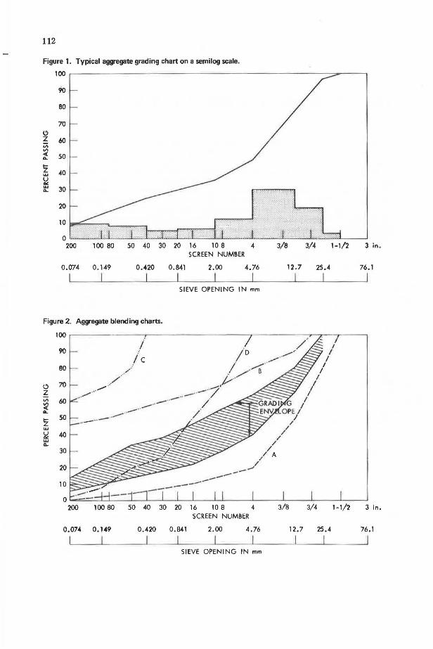
Gradation or particle size distribution of an aggregate can be expressed in terms of total percentages, by weight, passing each sieve of a series; total percentages retained on each sieve; or percentages passing one sieve and retained on the next (size fractions). The nature of particle size distribution can be examined by graphically representing the gradation by (a) a cumulative distribution curve on a semilog scale (Fig. 1), (b) the cumulative percentage passing versus the exponential function of the sieve size (1), or (c) a histogram or bar diagram of "percent fractions" among sieves and sieve sizes (Fig . 1).

The gradation specifications are usually in terms of upper and lower limits of total or cumulative percentages passing each sieve or percentages of fractions between successive sieves (percentage passing one sieve and retained on the next).

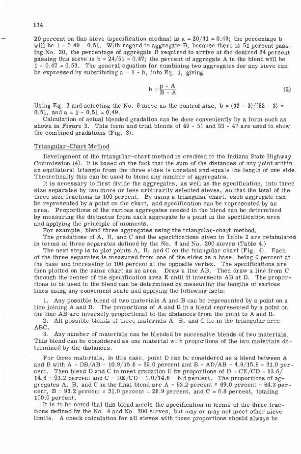
If the specifications are expressed in terms of the total percentage passing each sieve, they can be plotte d as bands or envelopes (Fig. 2). A method of transforming a "passing-retained" Specification to an approximate equivalent "total percentage pass­ing" specification was described by Dalhouse (2). The transformation enables the plot­ting of the passing-retained specification on the total percentage passing chart and makes visual examination and comparison of different specifications possible. How­ever, in this paper, all gradations and specification are expressed on a total percentage passing basis, unless otherwise stated.

GENERAL PROCEDURES

A large number of blending methods (techniques of determining relative proportions of various aggregates to obtain a desired gradation) have been developed since the

111

112

Figure 1. Typical aggregate grading chart on a semilog scale.

C) z ;;; V'I ,c( ... z w u ... w ...

100 .--------- ---- ----- -------- ----;;,,,-- - ~

90

80

70

60

50

40

30

20

10

100 80 50 40 30 20 16 10 8 SCREEN NUMBER

0.074 0.149 0.420 0.841 2.00 4.76

SIEVE OPENING IN mm

3 in .

12.7 25.4 76.1

Figure 2. Aggregate blending charts.

(j z

100 .------ ----.--- ----- ----,--------r-,.-- -,---~

90

BO

70

60

50

40

30

20

10

-/

/c ... ✓···/··

. / ' I D ./' ..,,,,..

/ ,,.,,,..---s··

... - J,,,·· ··--7' --4---_ .. --· / ' -·· . .-··- " / .. --··___,. .

0 --=;..._-'--.J_-....L.-.J_---1-_.__...__....,_..,_ __ ....,_ __ __._ __ __._ _ _ ___. _ _ _. 200 100 80 50 40 30 20 16 10 8 4 3/8 3/4 1-1/2 3 in.

SCREEN NUMBER

0.074 0.149 0.420 0.841 2.00 4.76 12.7 25.4 76.1

SIEVE OPENING IN mm

113

suggestion of "ideal gradation" by Fuller and Thompson (3). The suitability of these methods depends on the types of specifications and number of aggregates involved, the experiences of the individual, and the major emphasis of the blending (closeness to the desired gradation or economics).

Regardless of the number of aggregates involved or of the method to be used, the basic formula expressing the combination is

p = Aa + Bb + Cc +

where

(1)

p = the percentage of material passing (or retained on) a given sieve for the combined aggregates A, B, C, ... ;

A, B, C, = percentages of material passing (or retained on) the given sieve for aggregates A, B, C, ... ; and

a, b, c, = proportions (decimal fractions) of aggregates A, B, C, ... used in the combination and where a + b + c + ... = 1.00.

It is desirable, no matter which method is used, to first plot the gradations of the aggregates to be blended and the specification limits on a gradation chart (Fig. 2) be­fore actual blending is attempted. From these plots, decisions can be made prior to any calculation on (a) whether a blend(s) can be found using the available aggregates to meet the specification limits, (b) where the critical sizes are, and (c) if trial-and-error method is used, the approximate trial proportions to be selected. These decisions can be made based on the following simple facts:

1. The gradation curves for all possible combinations of aggregates A and B fall between curves A and B. It is impossible to blend aggregates C and B to meet the specification regardless of the method used (Fig. 2).

2. If two curves cross at any point (Band C, Fig. 2), the grading curves for all possible combinations pass through that point.

3. The curve for a blend containing more of aggregate A than Bis closer to curve A than B and vice versa.

REVIEW OF MAJOR BLENDING TECHNIQUES

In the following sections, six major blending methods and their variations are re­viewed using examples. For clarity and ease of comparison among methods, only three blending problems involving blending of two, three, and four aggregates to meet respective gradation specifications (Tables 1, 2, and 3) are used .

Trial-and-Error Method

As the name implies, in this method, trial blends are selected (aided by experience and plots of individual gradation curves and specification) and calculated for each sieve for the combined grading (using Eq. 1). The grading that results is compared with the specification. Adjustments can be made for the second or the third trial blends and the calculations repeated for the critical sieves until the satisfactory or optimum blend is obtained. This method, guided by a certain amount of reasoning, mathematics, and graphics , is the easiest procedure to determine a satisfactory blend for two or even three aggregates.

For example, blend aggregates using the trial-and-error method (problem 1, Table 1). Examination of grading curves indicates that it is possible to find a blend that falls

within the specification limits, possibly a 50- 50 blend because of the relative distance of the curves to the center of the band. The first trial blend can be determined more intelligently if certain critical sizes or control sizes are selected. By inspecting the gradations, it can be noted that all fractions re tained on the 3/a-in. sieve (100 - 80 = 20 percent) have to come from aggregate A and all that are less than the No. 30 aggregate mus t be furnishe d by agf regate B. With regard to aggregate A, because 100 - 59 = 41 pe rcent retained on the 1/a-in . sieve from A, the percentage needed fr om A to retain

114

20 percent on this sieve (specification median) is a = 20/ 41 = 0.49; the percentage b will be 1 - 0.49 = 0.51. With regard to aggregate B, because there is 51 percent pass­ing No. 30, the percentage of aggregate B required to arrive at the desi red 24 percent passing this sieve is b = 24/51 = 0 .47; the percent of aggregate A in the blend will be 1 - 0.47 = 0. 53. The general equation for combining two aggregates for any sieve can be expressed by substituting a = 1 - b, into Eq. 1, giving

Using Eq. 2 and selecting the No. 8 sieve as the control size, b = (43 - 3) / (82 - 3) 0.51, and a = 1 - 0.51 = 0.49.

(2)

Calculation of actual blended gradation can be done conveniently by a form such as shown in Figure 3. This form and trial blends of 49 - 51 and 53 - 47 are used to show the combined gradations (Fig. 3).

Triangular-Chart Method

Development of the triangular-chart method is credited to the Indiana State Highway Commission (4). It is based on the fact that the sum of the distances of any point within an equilateraCtriangle from the three sides is constant and equals the length of one side. Theoretically this can be used to blend any number of aggregates.

It is necessary to first divide the aggregates, as well as the specification, into three size separates by two more or less arbitrarily selected sieves, so that the total of the three size fractions is 100 percent. By using a triangular chart, each aggregate can be represented by a point on the chart, and specification can be represented by an area. Proportions of the various ag{!:regates needed in the blend can be determined by measuring the distances from each aggregate to a point in the specification area and applying the principle of moments.

For example, blend three aggregates using the triangular-chart method. The gradations of A, B, and C and the specifications given in Table 2 are retabulated

in terms of three separates defined by the No. 4 and No. 200 sieves (Table 4.) The next step is to plot points A, B, and C on the triangular chart (Fig . 4) . Each

of the three separates is measured from one of the sides as a base, being 0 percent at the base and increasing to 100 percent at the opposite vertex. The specifications are then plotted on the same chart as an area. Draw a line AB. Then draw a line from C through the center of the specification area E until it intersects AB at D. The propor­tions to be used in the blend can be determined by measuring the lengths of various lines using any convenient scale and applying the following facts:

1. Any possible blend of two materials A and B can be represented by a point on a line joining A and B. The proportions of A and Bin a blend represented by a point on the line AB are inversely proportional to the distances from the point to A and B.

2. All possible blends of three materials A, B, and C lie in the triangular area ABC.

3 . Any number of materials can be blended by successive blends of two materials. This blend can be considered as one material with proportions of the two materials de­termined by the distances.

For three materials, in this case, point D can be considered as a blend between A and B with A= DB/ AB= 10 .9/ 15.8 = 69.0 percent and B =AD/ AB = 4.9/ 15 .8 = 31.0 per­cent. Then blend D and C to meet gradation E by proportions of D =CE / CD= 13.6/ 14.6 = 93.2 percent and C = DE / CD = 1.0/14.6 = 6.8 percent. The proportions of ag­gregates A, B, and C in the final blend are A = 93 .2 percent x 69.0 percent = 64.3 per­cent, B = 93.2 percent x 31.0 percent= 28.9 percent, and C = 6.8 percent, totaling 100.0 percent.

It is to be noted that this blend meets the specification in terms of the three frac­tions defined by the No. 4 and No. 200 sieves, but may or may not meet other sieve limits. A check calculation for all sieves with these proportions should always be

Table 1. Blending of two aggregates, Table 2. Blending of three aggregates, problem problem 1 (based on percentage passing). 2 (based on percentage passing).

Aggregate Aggr egate Median of

Sieve Size A B Specification Specifications Sieve Size A B

1/~ in. 100 100 100 100 1 ln . 100 100 1/2 in. 90 100 80 to 100 90 ½ rn. 63 100 1/~ in. 59 100 70 to 90 80 No . 4 19 100

No 4 16 96 50 to 70 60 No. 10 8 93 No , 8 3 82 35 to 50 43 No. 40 5 55 No , 30 0 51 18 to 29 24 No. 80 3 36 No , 50 0 36 13 to 23 18 No. 200 2 3 No. 100 0 21 8 to 16 12 No , 200 0 9 4 to 10 7

Figure 3. Trial-and-error calculations for problem 1.

Iowa State University Civil Engineering Materials l..boratory

Aggregate Blending

C Specifi cation

100 94 to 100 100 70 to 85 100 40 to 55 100 30 to 42 100 20 to 30

97 12 to 22 88 5 to 11

Median of Specifications

97 78 48 36 36 17

8

Design to meet. ___ _ Date. _ _ ______ _

Specification Operator ______ _ No. ____ _

A B

< ., -~ ,0

"' -" . "' . lf ~ i lf ~ .... ,i ! i g'

lf .. . lf "°gi ~

" .. ] ~ ... ~~ ! ... ~

-~ 3 .... < 3 3 3 3 ... <( ... • .... g II) II) .. ., <( ., < Ill .. e •rl E'3 :i II) ....

.,,... :l';l., =~ m ~3 ... .... II) 0 • II) 0 •

~ ~ ~ .,

0,; ., ., ., 0 • .,

~ g' " ... ., :i ., : ! .. : : p.. ~ :;:! .... i =-~ p.. ...... ., p.. ... 8. ~ .... 0 .... ~ ~ ~ ;': .... ~ ., .... ~t: ~~ .... ~ ti .... ~ <fJ:Z: ~ .. ... ... .... p.. ~E-< E-< ...... ti).-<

0.4 49 .0 0 .5 51.0 100 3/4 100 0.5 53,0 100 0.4 47.0 r,nn 100

1,,1,, l 51 C las 1/2 90 1,,7 .7 100 47.0 la1,, 80-10 ~

?A .9 51.0 179 3/8 59 31. 3 100 47.0 78. 70-90

7 8 49 .0 !56 . 4 16 8.5 96 45.l Is~ 50-70

l 5 41 8 '1,, ~

8 3 1 r.. 82 38 5 11,,n 35-50

0 26.0 6.0 30 0 0 51 ?I,, 0 !4 . 0 18-29 .

0 18. 4 A .i.

50 9 0 36 16.9 6,9 13-23

n 10 7 LO 7 100 0 0 21 9.9 9.8 8-16

n 4 6 I,, ~

200 0 0 9 4.2 4 ~ 4-10

115

116

done. A calculation of the gradation of the blend by these proportions indicates that the blend meets specification limits for all sieve sizes (Table 5).

Ranges of percentages for aggregates A, B, and C can be determined by plotting lower and upper limits of the specification on Figure 4 as L and M and determining pe rcentages of A, B, and C for Land for M separately (5). To improve the likelihood of the proportions d~termined from the triangle chart defined by two sieves or three fractions to meet requirements of other sieves, two procedures can be used as follows:

1. Select the two control s i eves by comparing the steepness of the grading curves, so that the sum of the coarse fraction of coarse aggregate (i.e., A in this example), medium fraction of medium aggregate (aggregate B), and fine fraction of the fine ag­gregate (C) is a maximum (6). For the materials in this example, sieves No. 8 and No. 200 may be chosen because the sum is 90 + 92 + 88 = 270 as compared to the sum of 81 + 97 + 88 = 266 for sieves No. 4 and No. 200.

2. The procedures can be repeated using a second or third triangle chart, each time using different control sieves to divide the aggregates and specification into three fractions and each time determining the ranges of needed materials. By comparing the lower and upper limits determined from different triangle charts , ranges of materials can be determined that meet the limits of all sieves selected.

Modifi d Tria.ngular - ChaJ·t Methods

Modified triangular-chart methods were introduced by Driscoll (7) and Aron (8) by which one solution, showing all possible blends of three aggregates;- can be obtained graphically. Though no calculation or guesswork is needed and steps are simple to follow, the procedures are quite cumbersome, especially if more sieves are involved in the specifications.

To find the most economical blend, "iso-cost" lines ("isopleths") can be drawn either on the blending chart or on a separate transparent triangular chart.

Rectangular-Chart or Straight-Line Method

The rectangular-chart method is possibly the best method for blending two aggre­gates because it is simple, it requires no computation, it considers all sieve require­ments at once, and it provides solutions for all possible blends that will aid in selec­tion of the most economical blend. Even though the procedure can be used to blend three or more aggregates, repeated trials may be necessary, and there is no assur­ance of obtaining the optimum or the most economical blend.

Example 1-Blend two aggregates (Table 1) using the rectangular-chart method. T his method is illustrated in Fi gure 5, which shows a diagram with vertical per­

centage scales for the two aggregates and horizontal scales for proportions of aggre­gates in the blend. Gradation of aggregate A is represented by points on a 100 percent A vertical scale; gradation of aggregate B is plotted on a 100 percent B (0 percent A) scaie. Points on ihe vertical scales con1nion to the same sieve sizes are connected and labeled. This line will contain all possible percentages of that size material for any blend of A and B . A vertical line intersecting any sloping line indicates that the blend of A and B, as measured from horizontal scales, will yield a mixture with a percentage passing that sieve as indicated by the vertical scales.

For a particular sieve size, specification limits are indicated on the sloping line. That portion of the line between the two points represents the proportions of aggregates A and B, measured on the horizontal scale, that will meet specification limits for that sieve. When all specification limits on all sieves are plotted and points of lower and upper limits of consecutive sieves are connected, a specification envelope will be formed by which all possible blends can be defined. In this example , 43 to 55 per­cent A and 45 to 57 percent B will meet the specifications when blended. If the mid­point of all possible blends is selected, the best blend will be 49 percent A and 51 per­cent B. The gradation of the blend can be read directly off the vertical scale, as indicated by the points of intersections of the vertical line and the respective sieve sloping lines.

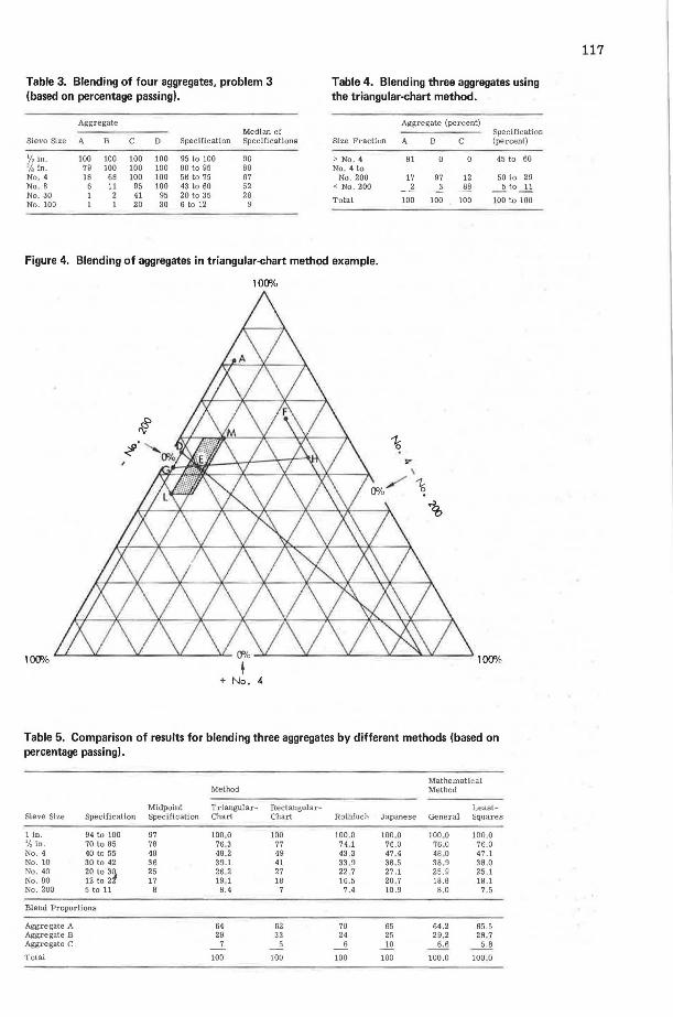
Table 3. Blending of four aggregates, problem 3 Table 4. Blending three aggregates using (based on percentage passing). the triangular-chart method.

Aggregate Aggregate (percent) Median of Specification

Sieve Size A B C D Specification Specifications Size Fraction A B C (percent)

/J2 in. 100 100 100 100 95 to 100 98 > No. 4 Bl 0 0 45 to 60 1/, In. 79 100 100 100 BO to 95 BB No, 4 to No. 4 18 68 !00 100 58 to 75 67 No. 200 17 97 12 50 to 29 No . B 6 11 95 100 43 to 60 52 < No. 200 2 3 ~ ___E. to 11 No. 30 1 2 41 95 20 to 35 28

Total 100 100 100 100 to 100 No. 100 1 1 20 30 6 to 12 9

Figure 4. Blending of aggregates in triangular-chart method example.

100'/o

lO<J>/o lO<J'/c

+ No. 4

Table 5. Comparison of results for blending three aggregates by different methods (based on percentage passing).

Mathematical Method Method

Midpaint Triangular- Rectangular- Least-Sieve Size Specification Specification Chart Chart Rothfuch Japanese General Squares

1 ln. 94 to 100 97 100,0 100 100 ,0 100.0 100.0 100.0 ½ in. 70 to 85 78 76 .3 77 74 .1 76.0 76 .0 76.0 No. 4 40 to 55 48 48.2 49 43.3 47.4 48 ,0 47.1 No. 10 30 to 42 36 39.1 41 33 .9 38 .5 38 ,9 38.0 No. 40 20 to 3~ 25 26 ,2 27 22.7 27.1 25.9 25.1 No. BO 12 to 2 17 19. 1 18 16.5 20 .7 18.8 18.1 No. 200 5 to 11 B 8.4 7 7.4 10.9 8.0 7.5

Blend Proportions

Aggregate A 64 62 70 65 64.2 65.5 Aggregate B 29 33 24 25 29 ,2 28.7 Aggregate C 7 5 6 ...!Q ___!& 2J! Total 100 100 100 100 100.0 100 ,0

117

118

Two ingenious procedures for using this method, for repeated blending of two ma­terials to meet different specifications or repeated blending of two different materials to meet one given specification, have been suggested ~. 10).

Example 2-Blend three aggregates (Table 2) using the rectangular-chart method. When more than two aggregates are to be combined and the rectangular-chart method

is used the best combinations of two of the materials must first be selected on one chart as previously described. This combination is then considered as a single ag­gregate, and its combination with a third material is determined in the same way on a second chart. The procedure is illustrat d by solving this p1·oblem as follows (Fig. 6):

1. Plot gradations of aggregates A, B, and C on scales A B, and C. 2. Connect the percentage passing for each respective sieve size by straight lines

between scales A and B. Mark on each sieve line the specification limits for that par­ticular sieve.

3. Choose a vertical line that will strike the best average between the specification limits. In this example, the vertical line selected represents 65 percent A and 35 per­cent B.

4. Project horizontally the intersections of each sieve line with the selected vertical line to scale A. The values projected on scale A represent the gradation for an aggre­gate blend composed of 65 percent aggregate A and 35 percent aggregate B.

5. Repeat steps 2 and 3 to determine the final proportions for blending aggregate C with the combination of aggregates A and B. In this example, the vertical line chosen represents 5 percent aggregate C and 95 percent aggregates A and B, or aggregate C = 5 percent, aggregate B = 0.95 x 35 percent = 33 percent, and aggregate A ,,. 0.95 per­cent x 65 percent = 62 percent totaling 100 percent.

6. The gradation of the final bl~nd can be obtained by horizontally projecting the intersections of each line with the selected vertical lipe (Table 5).

Rothfuchs' Balanced Area Method

The method developed by Rothfuchs (11-13) is widely used outside the United States and has been considered in many countries as one of the most useful graphical proce­dures. It is reasonably quick and simple and can be applied to mixtures of any number of aggregates .

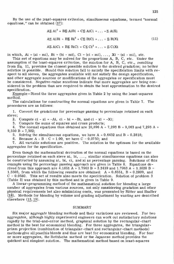
For example, plend three agg1:egates (Table 2) using the Rothfuchs method. The solution and procedure, shown in Figure 7, a.re as follows:

1. Plot the median or midpoint of the specifications using linear ordinates for the percentage passing, but choose a scale of sieve size such that the grading plots as a straight line. Tllis can be done readily by drawing an inclined line, S, and marking on it the sizes corresponding to the various percentages passing.

2. The gradings of aggregates A, B, and Care plotted on this scale (curves A, B, and C).

3. Straigh· lines fual most nea1°ly approximate the grading curves of the individual aggregates are drawn (lines A~ B ~ and C'). This is done by selecting a straight line for each curve such that the areas enclosed between it and the curve are a minimum and are balanced about the straight line.

4. The opposite ends of these straight lines are joined together; the propol'tions for the blend can be read off from the points where these joining lines intersec the straight line representing the specification irrading (P 1 and P 3). Figure 7 shows that this method yields the following proportions: aggregate A = 70 percent, aggregate B = 24 percent, and aggregate C = 6 percent, totaling 100 pe1·cent. The grading for tllis combination is given in Table 5.

It is to be noted that calculations using the proportions determined graphically are necessary and that the blend may or may not meet the specification. The only case in which the blend determined from the ehart yields the exact specification grading (S) is when (a) all agg1·egate grading curves are linear as plotted on the cha.rt and (b) there is neither gap nor overlapping among the aggregates; i.e. , the opposite ends of the st1·aight gradation lines of the aggregates can be joined by vertical lines as shown in Figure 8.

Figure 5. Blending two aggregates by straight-line chart method.

A % B B - 0

20 40 60 80 100

80

(!) z 60

<( -V'I

~< <( Q..

~z 40 <><w

l!lu '-'~ <( Q..

20

80 60 40 20 0

%A

Figure 6. Blending three aggregates by rectangular-chart method.

'-' z V'> V'> <( 0..

..... z w u "' w 0..

C

0 100

~

80 I"'-.

60

40

20

0 100

% Agg. A + Agg. B A 0

100 20 40 60

;;:--- I/, .

~ ~ -..:.!.!.:..., -t----..

""' ~ ~ ~ ' "' "" ~ " ~ ""' " 0 " "- f.,.,t

"' " ~ "-' '%

80 60 40

% Agg. C

20 80

-- ~- --............ .....--

,4

~ r-...... -(a I~ ..... ~.., ~ I""-. / .JV

~ ""' "", // V

~

20

' /

,~ 0

100

/ / ,,,- ~

_..-

80

c0 z w 0 ..... ,_ <( (!)

<( u w u:: "" (!) u

(!) LU

<( Q.. V,

% Agg . B 40 60 80

,., \~•

----v _:,.,,,- / .. ,, i..,...-

-2J / / "~

/ 1J,-"'

V I/ / ~ / -

B 100

V V

./

./ y

-~ . _v--V ~_!)!!- I--"'"

----No. ')()('

60 40 20 0 % Agg. A

119

120

Japanese Method.

A method, recommended by the Japanese Highway Institution (14) , is based on a concept similar to that of Rotb.fuchs' method . In the Japanese method, a straight-line specillcation median and aggregate gradings are plotted as described in Rothfuc hs' method. But instead of approximating the grading curves to straigh t lines, vertical lines are drawn between the opposite ends of adjacent curves so that, if tile two grada­tions overlap, the percentage retained on the upper curve equals the percentage passing on the lower curve (curves A and B, Fig. 9), and, if there is a gap between the two gradations curves, the horizontal distances from the opposite ends of the curves to the vertical line are equal (curves C and D, Fig . 9) . Again, the proportions for the blend can be read off from the point where these vertical lines cross the specification median. This method is shown in Figure 9.

Example 1-Blend three aggregates (Table 2) using the Japanese method . The solution for this problem is shown in Figure 10. This gives the following pro­

portions : aggregate A = 65 percent, aggregate B = 25 percent, and aggregate C : 10 percent, totaling 100 percent. The r esulting gradation of the blend was calculated and is given in Table 5.

It has been demonstrated (13) that the plotting of gradations on a straight-line spec­ification scale is not necessary in the Japanese method. Identical results can be ob­tained if vertical lines between adjacent a ggregate grading cu-rves are drawn on a reg­ular semllog gradation chart.

Example 2-Blend four aggregates (Table 3) using the modified Japanes e method . The blending is shown in Figure 11. The grading of the blend is given in Table 6.

Though the Japanese method is very quick, simple, and exact, it is less reliable than Rothfuchs' method. However, the latter method is not exact because of tile judgment factor involved when straight lines are drawn to approximate the grading curves of the individual aggregates. In either case, adjustments of the proportions obtained graph­ically may have to be made when sieve-by-sieve comparison between the gradation of the blend and the specification is examined .

Projection-Triangular Chart or T1•iangle-Rec tangular Chart Method

A method using a combination of rectangular -chart and triangular-chart techniques for an economical blend of three aggregates was developed independently by Sargent (15) and Sheeler (16). In both approaches, the possibilities of blending two aggregates at a time to meet certain sieve limits are evaluated on rectangular charts . The ranges for each sieve are plotted on a triangular chart as an area. The common area enclosed by ranges for all sieves represents all possible blends of the three aggregates that will meet the specification.

Sars;rent 's Method

The procedure for this method is illustrated first by blending three aggregates to meet a hypo thetical specification in terms of limitations by only one sieve size (Fig. 12) and then by solving problem 2 (Table 2 and Fig. 13). In Figure 12, the blending problem is as follows:

Sieve Size

No. 4

Agg1·egate Gradations (percent) A B C

60 30 10

Specification (percent)

40 to 50

The ranges 01 proportions that will mee t the specifications with respect to the No. 4 sieve (as indicated by the shaded area) are aggregate A = 33 to 82 percent, aggregate B = 0 to 67 percent, and aggregate C = 0 to 40 percent.

The ranges of proportions that will meet the specifications of problem 2 are as fol ­lows (shaded areas in Fig. 13): aggregate A = 62 to 74 percent, aggregate B = 16 to 36 percellt, and aggregate C = 4 to 10 percent.

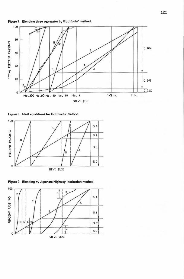
Figure 7. Blending three aggregates by Rothfuchs' method.

100 ,--,--:::-r---:::;;.,-...-------,--,----=:....-----------~--------,~

80 (!) z ;;; ~

60 "-

z w u D< w 40 "-...J <( .... 0 .... 20

No.200 No.SO No. 40 No. 10 No. 4

SIEVE SIZE

Figure 8. Ideal conditions for Rothfuchs' method.

SIEVE SIZE

Figure 9. Blending by Japanese Highway Institution method.

(!) z "' ~ "-

2 ... u 115 "-

SIEVE SIZE

1/2 in. in.

121

Figure 10. Blending three aggregates by Japanese Highway Institution method.

100

80 / 1

0 / I z B . I V, ./ I VI < I I ... 60 z I w u I "' I w ... 40 ...I

< .... 0 ....

20 _,,./

0 No. 200 No.BO No. 40 No.10 No. 4

SIEVE SIZE

Figure 11. Blending four aggregates by modified Japanese method.

100

90

80

0 z 70 vi V'I < 60 ... .... z

50 w u m ... -40 ...I

< 6 30 ....

20

10

0

, .. --, I I .. , I

I I { I I , . J

o/

/ _/ /

/ '

1 5 10 20 -400270200 100 50 30 16 SIEVE SIZES

1 5 10 20 50 100 500 1000 log SCALE I I I I I I I I AVERAGE I I I I I I I CLEAi 0.00005 0.0001 0.0005 0.001 0.005 0 .01 0.05 OPENING

Table 6. Comparison of results for blending four aggregates by different methods (based on percentage passing).

Steve Size Specification

½ in. 95 to 100 % in. 80 to 95 No. 4 58 to 75 No. 8 43 to 60 No. 30 20 to 35 No. 100 6 to 12

Blend Proportions

Aggregate A Aggregate B Aggregate C Aggregate D

0.65A

0.258

0.10C

1/2 in . ir.

0.30A

0.208

0 . 30C

0.20D

B 4 3/B 3/4 1-1/"1 3 in . SQUARE :JPENING

5000 10000 50000 MICRONS

' I I

' 0., 0.5 2 3 in.

Method Median Specification Japanese Rothiuch Mathematical

98 100,0 100.0 100 88 93 ,7 95.2 92 67 69.0 72.5 65 52 52,5 51 ,2 53 28 32,0 24.0 27

9 12 .6 11.0 11

30 23 38,8 20 27 9,5 30 45 42 ,9 20 5 9.0

Figure 12. Blending three aggregates to meet one-size specification by Sargent's method.

100 100

100'----------------' 100

Figure 13. Blending three aggregates by Sargent's method.

100 • A 100

100

Agg. C

100

1/2 in . No . 4

No. 10 No . 40

No . 80 No . 200

100

124

Mathematical Method

General Equations-As stated previously, the basic equation for aggregate blending is

aA + bB + cC + . . . = S (3)

which can be obtained for each sieve . In this equation, Sis the percentage either pass­ing or retained on the particular sieve for the midrange of specification limits. Thus, for two aggregates , the equations will be (for sieve i)

aAi + bBi = Si (4)

and

a+b = l (5)

For blending three aggregates, the following simultaneous equations can be obtained for control sieves 1 and 2: aA 1 + bB1 + cC 1 = S1, aA2 + bB2 + cC 2 = S2 , and a + b + c = 1.

Example-Blend the three aggregates given in Table 2 using the mathematical method. F or percentages retained on the No. 4 sieve,

81a +Ob+ Oc = 52

For percentages passing the No . 200 sieve,

2a + 3b + 88c = 8

Also,

a+b+c=l

(6)

(7)

(8)

Solving Eqs . 6, 7, and 8 for a , b, and c yields a= 0.642, b = 0.292, and c = 0 .066. It is obvious that s olutions for the simultaneous equations can meet the requirem ents

of only n - 1 sieves, with n being the number of aggregates in the blend. Therefore, check calculations for all other sieves in the specifications are necessary. Gradations of the blend with the preceding proportions are computed and given in Table 5.

Least-Squar es Method- Least-squares method, developed by Mackintosh (§) and Neumann (17), pr ovides the best possible blend from the available aggregates by con­structing simultaneous normal equations with unique solutions. The equations are con­structed based on fractions retained on each sieve and minimization of the sum of the squared residual terms for all sieves.

Assume that M aggregates are to be blended to meet midpoint specification X and that the proportion (in decimal fractions) of each aggregate to produce the desired blend will be A, B, C, . .. , M for aggregates A, B, C, . . . , M respectively . M represents the last aggregate; therefore, we have

A + B + C + ... + M = 1.00 (9)

and

A, B, C, ... , M;;,: 0. (10)

Let the percentage retained on each of the n sieves in the gradations for the first aggregate be al, a2, a3, ... , ai, ... , an; for the second aggregate bl, b2, b3, ... , bi, ... , bn; and for the last aggregate ml, m2, m3, ... , mi, ... , mn, etc., where the subscript indicates an arbitrarily assigned sieve number . The percentage retained on each sieve for the specification median is xl, x2, x3, ... , xi, ... , xn .

125

By the use of the least-squares criterion, simultaneous equations, termed "normal equations," can be obtained (17):

A~ Ai2 + BI: AiBi + CE AiCi + ... =I: AiXi

Ar; AiBi + BI: Bi2 + CE BiCi + ... = E BiXi (11)

AI: AiCi + BE BiCi + Cr; Ci 2 + ... = E CiXi

in which, Ai = (ai - mi), Bi = (bi - mi), Ci = (ci - mi), ... , Xi = (xi - mi), etc. This set of equations may be solved for the proportions A, B, C, etc. Under the

assumption of the least-squares criterion, the solution for A, B, C, etc., resulting from Eq. 11, provides the closest possible solution to the desired gradation; no better solution is possible. Should this solution fail to satisfy the specification limits with re­spect to all sieves, the aggregates available will not satisfy the design specification, and other aggregate sources or modifications of the aggregates or specification must be considered. Negative-value solutions indicate that more aggregates are being con­sidered in the problem than are required to obtain the best approximation to the desired specification.

Example-Blend the three aggregates given in Table 2 by using the least-squares method.

The calculations for constructing the normal equations are given in Table 7. The procedures are as follows:

1. Convert the gradations for percentage passing to percentage retained on each sieve;

2. Compute ci - ai = -Ai, ci - bi= -Bi, and ci - xi= -Xi; 3. Compute the sums of squares and cross products; 4. The normal equations thus obtained are 10,896 A+ 7,293 B = 9,063 and 7,293 A+

9,550 B = 7,382; 5. Solving the simultaneous equations, we have A= 0.6432 and B = 0.2818; 6. Because A+ B + C = 1.00, we have C = 0.0750; and 7. All variable solutions are positive. The solution is the optimum for the available

aggregates for the specification.

Even though the mathematical derivation of the normal equations is based on the percentage retained on each sieve ai, bi, ... , similar simultaneous equations can also be constructed by assuming ai, bi, ci, and xi as percentage passing. Solutions of this example using the percentage passing approach are given in Table 8. Equations de­rived from this approach are 4.1651 A+ 1.7963 B = 3.2439 and 1.7963 A+ 1.3020 B = 1.5503, from which the following results are obtained: A = 0.6551, B = 0.2809, and C = 0.0580. This set of results also meets the specification. Solution of problem 3 (Table 3) was obtained by this method and is given in Table 9.

A linear-programming method of the mathematical solution for blending a large number of aggregates from various sources, not only considering gradation and other physical requirements but also minimizing costs, was presented by Ritter and Shaffer (18). Methods for blending by volume and grading adjustment by wasting are described elsewhere (13,~).

SUMMARY

Six major aggregate blending methods and their variations are reviewed. For two aggregates, although highly experienced engineers can work out satisfactory solutions rapidly by the trial-and-error method, graphical solution by the rectangular-chart method is the best for economical blending. For three aggregates, the triangular­prism projection (combination of triangular-chart and rectangular-chart methods) methods give all possible blends and thus are best for economical blending. For four or more aggregates, the Rothfuchs method or the Japanese method provides the quickest and simplest solution. The mathematical method based on least-squares

Table 7. Blending three aggregates by least-squares method (based on percentage retained).

Gradation

Aggregate Value Midpoint

A B C SpecU1catton -Al -Bi -Xi Sieve Size {al) (bi) (ct) [X(xl)] (ci • ai) (cl - bl) (cl - xi) Al1 AJBi AIXi Bl' BiXI

1 in. 0 0 0 3 0 0 -3 0 0 0 0 0 '/2 In . 37 0 0 19 -37 0 - 19 1,369 0 703 0 0 No. 4 44 0 0 30 -44 0 -30 1,936 0 1,320 0 0 No. 10 11 7 0 12 -11 -7 - 12 121 77 132 49 84 No. 40 3 38 0 II -3 -38 • 11 9 114 33 1,444 418 No. 80 2 19 3 8 1 -16 -5 I -16 -5 256 80 No. 200 l 33 9 9 8 -24 0 64 -192 0 576 0 Pan 2 ...1 88 8 86 85 80 7,396 !d.!Q 6,880 7,225 6,800

Total 100 100 100 100 10,896 7,293 9,063 9,550 7,382

Note: 10,896 A+ 7,293 8 aa 9,063; 7,293 A+ 9,550 8 ,. 7,382; and A+ B + C = 1, A • 0 .6432, B • 0 2818, and C = 0 0750

Table 8. Blending three aggregates by least-squares method (based on percentage passing).

Gradation Value

Aggregate Specification -Al -Bl -XI

Sieve Size A B C (X) (C • A) (C • B) (C - X) Al' AlBI A!Xi Bf BiXf

1 in. 100 100 100 97 0 0 0.03 0 0 0 0 ,0 '12 in . 63 100 100 78 0.37 0 0.22 0.1369 0 0.0814 0 0 No. 4 19 100 100 48 0.81 0 0.52 0.6561 0 0.4212 0 0 No. 10 B 93 100 36 0,92 0 .07 0.64 O.B464 0.0644 0.5B8B 0.0049 0.044B No. 40 5 55 100 25 0.95 0. 45 0.75 0 .9025 0.4275 0.7125 0.2025 0.3375 No. BO 3 36 97 17 0.94 0,61 0,80 0.8836 0.5734 0.7520 0.3721 0.4880 No. 200 2 3 88 8 O.B6 0 ,85 0,80 ~ 0.7310 0.6880 ~ ~ Total 4.1 651 1.7963 3.2439 1.3020 1.5503

Note: AtAi2 + BtAiBi • tAiXi, A!AiBi + BI:8i2 = I:BiXi, and A+ B + C = 1.(Xl, A -- 0,6551, B • 0.2869, and C • 0,0580.

Table 9. Blending four aggregates by least-squares method.

Desired Value Aggregate Specifi-

Sieve cation -Ai -B! -Ci · XI Size A B C D (X) (n - A\ (D · B) (B-C) (D · X) Al' AiBi AJCI AJXI Bl ' BICI B!Xl Cl' CIXI

½in. 100 100 100 100 98 0 0 0 0.02 0 0 0 0 0 0 0 0 0 % in. 79 100 100 100 88 0 ,21 0 0 0 ,12 0.0441 0 0 0.0252 0 0 0 0 0 No. 4 18 68 100 100 67 0.82 0.32 0 0.33 0 .6724 0,2624 0 0.2706 0.1024 0 0. 1056 0 0 No. 8 6 11 95 100 52 0.94 0.89 0.05 0.48 0.8836 0.8366 0.0470 0.4512 0.7921 0 .0445 0.4272 0.0025 0.024 No. 16 2 3 60 100 No. 30 1 2 41 95 28 0 .94 0.93 0.54 0 .67 0.8836 0.8742 0.5076 0.6298 0.8649 0.5022 0.6231 0.2916 0.361 No. 50 1 2 31 86 No. 100 1 l 22 39 No. 200 1 1 20 30 0 .29 0.29 0.10 0.21 0.0841 .2.:.Q.!!!!. 0.0290 0.0609 0.0841 0.0290 0.0609 0.0010 0.021

Total 2. 5678 2.0573 0.5836 1.4377 1.8435 0.5757 12168 0.2951 0 .408

Note: 2.5678 A+ 2.0573 B + 0 5836 C = 1 4377; 2.0573 A+ 1,8435 B + 0.5757 C • t 2168; 0 5636 A + 0.5757 B + 0,2951 C • 0 4068; and A+ B + C + 0 • 1,000 A• 0 386, B • 0,095, C • 0.429, and O • 0 .090.

127

criterion gives the best possible blend from all available materials. The linear­programming method of solution can be u_sed if minimizing costs is the major con­sideration a large number of aggregates of different characteristics are considered, other linear restrictions are placed in addition to gradation limits, and an electronic computer is readily available.

ACKNOWLEDGMENT

This work was supported in part by funds from the Engineering Research Ins titute, Iowa State University. The author thanks J. B. Sheeler, Department of Civil Engi ­neering, Iowa State University, for his critical review of the manuscript.

REFERENCES

1. Goode, J. F., and Lufsey, L. A. A New Graphical Chart for Evaluating Aggre­gate Gradations. Proc . AAPT, Vol. 31, 1962, p . 176 .

2. Dalhouse, J. B. Plotting Aggregate Gradation Specifications for Bituminous Con­crete. Public Roads, Vol. 27, No. 7, 1953, p. 155.

3. Fuller, W. B., and Thompson, S. E. The Laws of Proportioning Concrete. Trans. ASCE, Vol. 59, 1907, p . 76.

4. Spangler, M. G. Soil Engineering, 2nd Ed. 1960, p. 217, 5. Driscoll, G. F. How to Blend Aggregates to Meet Specifications. Engineering

News-Record, Jan. 5, 1950, p. 45. 6. Macltintosh, C. S. Blending of Aggregates for a Premix Carpet. Transvaal

Roads Department, Pretoria, 1959. 7. Driscoll, G. F. Graphical Method Simplifies Economical Blending of Aggregates.

EngineeringNews-Record, Sept. 21, 1961, p. 134. 8. Aron, G. Proportioning a Mix of Three Soils by Graph. Civil Engineering, Feb.

1959, p. 66. 9. Principles of Highway Construction as Applied to Airports, Flight Strips, and

Other Landing Areas for Aircrafts . U.S. Public Roads Administration, 1943. 10. Aaron, H. Stabilization Control on the Washington National Airport. HRB Proc.,

Vol. 21, 1941, pp. 515-530. 11. Roth[uchs, G. Graphical Determination of the Proportioning of the Various Aggre­

gates Required to Produce a Mix of a Given Grading. Betonstrasse, Vol. 14, No. 1, 1939, p. 12.

12. British Road Research Laboratory. Soil Mechanics for Road Engineers. Her Majesty 's Stationery Office, 1951, p. 227.

13. Fossberg, P. E. A Review of Methods for Aggregate Blending. National Institute for Road Research, Republic of South Africa, 1968.

14. Asphalt Pavement Concretes Handbook. Japanese Highway Institution, 1967. 15. Sargent, C. Economic Combinations of Aggregates for Various Types of Con­

crete. HRB Bull. 275, 1960, p. 1-17. 16. Sheeler, J. B. Private communication. 1972. 17. Neumann, D. L. Mathematical Method for Blending Aggregates. Jour. Con­

struction Div., ASCE, Vol. 90, No. 2, 1964, p. 1. 18. Ritter, J. B., and Shaffer, L. R. Blending Natural Earth Deposits for Least

Cost. Jour. Construction Div., ASCE, Vol. 87, No. 1, 1961, p. 39. 19. Mix Design Methods for Asphalt Concrete, 3rd Ed. The Asphalt Institute, 1969.