Rethinking the Effects of Fiscal Policy on Macroeconomic

*For helpful discussions, I thank Cem Karayalcin, Peter Thompson, Sheng Guo and Veysel Avsar.

**PhD Candidate, Department of Economics, Florida International University, FL 33199, USA. E-mail:

[email protected]

Rethinking the Effects of Fiscal Policy on Macroeconomic Rethinking the Effects of Fiscal Policy on Macroeconomic Rethinking the Effects of Fiscal Policy on Macroeconomic Rethinking the Effects of Fiscal Policy on Macroeconomic

Aggregates: A Disaggregated SVAR AnalysisAggregates: A Disaggregated SVAR AnalysisAggregates: A Disaggregated SVAR AnalysisAggregates: A Disaggregated SVAR Analysis****

Umut UnalUmut UnalUmut UnalUmut Unal********

First Draft---September 2011

AbstractAbstractAbstractAbstract

This paper characterizes the dynamic effects of net tax and government spending

shocks on prices, interest rate, GDP and its private components in four OECD countries using

a structural VAR approach. For the first time in this literature, I propose a structural

decomposition of total net taxes into four components: corporate income taxes, income taxes,

indirect taxes and social insurance taxes. The paper provides estimates of the responses of

macroeconomic aggregates to innovations in these net tax components. The main conclusions

of the analysis can be summarized as follows: 1) decompositions of total net tax innovations

show that net tax components have different impacts on economic variables; 2) the size and

persistence of these effects vary across countries depending upon the strength of wealth,

substitution, and income effects reflecting the structure of the economies; 3) positive tax

multipliers reported in previous studies are found only for the corporate income tax in the

US, Canada, and France and for the social security tax in the US; 4) while we find that private

investment is crowded out both by taxation and government spending in the UK and the US

as consistent with the neo-classical model, our results for France and partially for Canada,

indicate that there are opposite effects of tax and spending increases on private investment in

line with Keynesian theory; and 5) private consumption is crowded in by government

spending for all countries except the UK and crowded out by taxation in all countries except

France. While the former result is consistent with a Keynesian model, the latter is in line

with neo-classical theory.

JEL classification: E62; H20; H30

Keywords: Fiscal shocks; Structural vector autoregression; Tax policy

1

1.1.1.1. IntroductionIntroductionIntroductionIntroduction

A common approach in both empirical and theoretical studies on fiscal policy shocks

is to evaluate the response of macroeconomic aggregates to exogenous changes in the fiscal

policy variables. From a theoretical point of view, the impacts of discretionary fiscal policy

on the economy hinge on a number of key assumptions. For instance, in examining the

transmission mechanism of fiscal policy, the presence or absence of forward-looking

behavior plays a crucial role. If agents do not look forward, expected future changes do not

have any effect on current-period decisions. Agents with rational expectations, on the other

hand, do look forward in anticipation of future changes in key macroeconomic variables.

The empirical evidence, however, does not provide a common picture either. In

particular, even though the most recent and standard strand of the literature, which started

with Blanchard and Perotti (2002), shows positive short-term output multipliers resulting

from government expenditure increases and tax cuts, the estimated size and duration of these

effects vary across studies. In fact, the magnitude of the multiplier may depend on the

specification and/or sample period employed. Interestingly, there is even evidence of

negative government spending multipliers for Australia, Canada and the UK for some sub-

sample periods (Perotti, 2004).

There is a substantial body of literature devoted to the effects of fiscal policy on key

macroeconomic indicators using Structural Vector Autoregression (SVAR) models. For

instance, Alesina, Ardagna, Perotti and Schiantarelli (2002) investigated the effects of a

change in fiscal policy on private investment using a panel of OECD countries. Their finding

that increases in taxes have a negative impact on output is parallel to the findings of

2

Blanchard and Perotti (2002) 1. In addition, the latter concludes that private consumption

increases following an increase in tax rates.

Both of these studies demonstrate that any increase in taxes will reduce private

investment. Further, Perotti (2004) points out that the impact of any change in tax policy on

GDP and its components becomes weaker over time. Mountford and Uhlig (2008) try to

distinguish the effects of fiscal policy shocks for the US economy between 1955 and 2000.

They envisage three different scenarios: a deficit-financed spending increase, a balanced

budget spending increase, and a deficit-financed tax cut. They conclude that among these

three scenarios the deficit-financed tax cut is the most efficient one to help raise the GDP.

More recently, by employing a new database, Burriel et al (2010) analyze the effect of fiscal

policy for the US economy and Euro area as a whole. They find that GDP and inflation

increase in response to government spending shocks even though the output multipliers are

very similar and steadily increasing after 2000, possibly due to the “global saving glut”, in

both areas.

Alternatively, Burnside et al. (2004), Pappa (2009) and Ramey (2007) report a

decrease in unemployment in response to a positive spending shock. On the other hand, a

few studies consider the reaction of the real wage following an increase in government

spending. Among those, Pappa (2009) documents an increase whereas Burnside et al. (2004)

report a decrease in the real wage in response to an expansionary fiscal policy.

Some of the stylized facts above appear to contradict either neo-classical theory, real

business cycle (RBC) model or Keynesian approach. In other words, the sign and magnitude

of the effect of discretionary fiscal policy on macroeconomic aggregates often offers opposite

conclusions. For instance, following a positive government spending shock, New Keynesian

1 For a detailed discussion, see also Fatas and Mihov (2001), Tenhofen and Wollf (2007), De Castro and De Cos

(2008), Mertens and Ravn (2009) and Romer and Romer (2010).

3

theory tends to predict an increase in output, real wages and interest rate and a decrease in

consumption and private investment. Yet in RBC models, the expansionary fiscal policy will

lead to a decrease in real wages and an increase in private investment.

Additionally, economic theory suggests that different forms of taxation have different

impacts in macroeconomic activity. For instance, Barro (1990) points out that while non-

productive expenditures financed by a distortionary tax have an unambiguously negative

growth effect, non-distortionary tax-financed increases in productive expenditures are

predicted to have a positive impact upon the growth rate. Baxter and King (1993) point out

that financing government spending with lump-sum taxes and distortionary taxes have

different effects on economy. Gordon et al. (2004 and 2004a) analyze the impact on revenue

and costs of a substantial change in fiscal policy, such as the effects of switching from capital

income taxation to consumption-based tax system. They both find that consumption taxes

and income taxes have different impacts on saving and investment decisions.

In view of these discrepancies, the central message of this paper is that different tax

groups have different effects on macroeconomic aggregates, depending on the underlying

cause of the tax increase. Our results suggest that analyzing the fiscal policy by decomposing

total net taxes and examining their effect on the aggregate economy provide a more accurate

picture than treating total net taxes as the fiscal policy variable. To this end, under the

Blanchard and Perotti (2002) identification scheme, a five-variable VAR model, which

includes total government spending, total net taxes, GDP, a measure of inflation and the

interest rate is used as a benchmark for Canada, France, the UK and the US. Thereafter, I

propose a structural decomposition of total net taxes into four components: corporate income

taxes, income taxes, indirect taxes and social insurance taxes. The paper provides estimates of

the responses of macroeconomic aggregates to innovations in different tax groups by

replacing total net taxes with each tax components separately. In a further step, the responses

4

of the GDP components, private investment and consumption, to a shock to each tax

component will be examined.

Decompositions of total net tax innovations will help us assess the macroeconomic

implications of fiscal policy shocks for four major economies with different economic

structures. In this context, corporate income tax shocks, for instance, will have a very

different impact on macroeconomic indicators than an indirect tax innovation. It is,

therefore, important that we understand the extent to which increases in net taxes are driven

by one shock or another, before concerning ourselves possible policy responses.

The main conclusions of the analysis can be summarized as follows: 1)

Decompositions of total net tax innovations show that net tax components are found to have

different impacts on economic variables; 2) The size and persistence of effects vary across

countries depending upon different effects (i.e., negative wealth and output effects,

substitution effect and income effect) resulting from the structure of the economy; 3) The

positive tax multipliers reported in previous studies are found only for corporate income tax

in the US, Canada and France and for the social security tax in the US; 4) As regards macro

theories, we find that private investment is crowded out both by taxation and government

spending in the UK and the US which is consistent with a neo-classical model. On the other

hand, our results for France, and partially for Canada indicate that there are opposite effects

of tax and spending increases on private investment, which is in line with Keynesian theory;

and 5) Private consumption is crowded in by government spending for all countries except

the UK and crowded out by taxation in all countries except France. While the former result

is consistent with a Keynesian model, the latter is in line with neo-classical theory.

The remainder of the paper is organized as follows. Section II focuses on the

identification of the structural shocks. Section III describes the data. Section IV investigates

5

the impacts of the shocks identified in Section II on macroeconomic aggregates of four

countries. Section V analyzes the robustness of the results and section VI concludes.

2.2.2.2. The The The The Identification StrategyIdentification StrategyIdentification StrategyIdentification Strategy

Our identification strategy follows Blanchard and Perotti (2002). Denoting the vector

of endogenous variables by �� and the vector of reduced form residuals by ��, the reduced

form VAR can be represented as

�� = �� + �� (1)

where �� is a ��1 vector of endogenous variables, �� is a �� matrix lag polynomial,

and �� is a ��1 vector of reduced-form innovations which are assumed to be independently

and identically distributed with covariance matrix equal to the identity matrix. In our

benchmark specification �� and �� consist of the following variables: �� = [��, ��, �� , �� , ��]′

and �� = [��, ��

� , ��, ��

�, ��

�]′.

I start by expressing the reduced form innovations of the government spending and

net taxes equations as linear combinations of the structural fiscal shocks ��and ��

� to these

variables and the innovations of the other reduced form equations of the VAR, namely:

��, ��

� and ��

. This leads to the following formal representation of the reduced form

residuals:

�� = !�

��

+ !��

�+ !

�� + "�

��

+ �� (2)

��

= !��

�+ !�

��

�+ !

��

� + "��

� + �� (3)

As mentioned by Perotti (2004), in this framework, the coefficients !# measure both

the automatic response of fiscal variable $ to the macroeconomic variable % and the

6

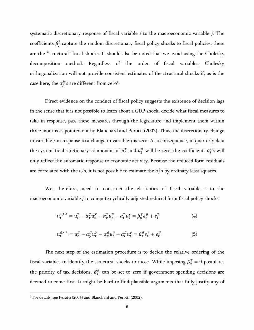
systematic discretionary response of fiscal variable $ to the macroeconomic variable %. The

coefficients "# capture the random discretionary fiscal policy shocks to fiscal policies; these

are the “structural” fiscal shocks. It should also be noted that we avoid using the Cholesky

decomposition method. Regardless of the order of fiscal variables, Cholesky

orthogonalization will not provide consistent estimates of the structural shocks if, as is the

case here, the !#&’s are different from zero2.

Direct evidence on the conduct of fiscal policy suggests the existence of decision lags

in the sense that it is not possible to learn about a GDP shock, decide what fiscal measures to

take in response, pass these measures through the legislature and implement them within

three months as pointed out by Blanchard and Perotti (2002). Thus, the discretionary change

in variable $ in response to a change in variable % is zero. As a consequence, in quarterly data

the systematic discretionary component of �� and ��

� will be zero: the coefficients !#

’s will

only reflect the automatic response to economic activity. Because the reduced form residuals

are correlated with the ��’s, it is not possible to estimate the !# ’s by ordinary least squares.

We, therefore, need to construct the elasticities of fiscal variable $ to the

macroeconomic variable % to compute cyclically adjusted reduced form fiscal policy shocks:

��,'( = ��

� − !��

�− !�

��

− ! ��

� = "��

�+ ��

� (4)

��,'(

= ��

− !��

�− !�

��

�− !

��

� = "��

� + �� (5)

The next step of the estimation procedure is to decide the relative ordering of the

fiscal variables to identify the structural shocks to those. While imposing "�� = 0 postulates

the priority of tax decisions, "�� can be set to zero if government spending decisions are

deemed to come first. It might be hard to find plausible arguments that fully justify any of

2 For details, see Perotti (2004) and Blanchard and Perotti (2002).

7

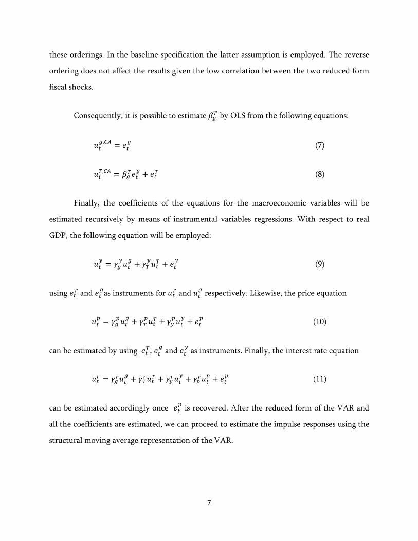
these orderings. In the baseline specification the latter assumption is employed. The reverse

ordering does not affect the results given the low correlation between the two reduced form

fiscal shocks.

Consequently, it is possible to estimate "�� by OLS from the following equations:

��,'(

= �� (7)

��,'( = "�

��

+ �� (8)

Finally, the coefficients of the equations for the macroeconomic variables will be

estimated recursively by means of instrumental variables regressions. With respect to real

GDP, the following equation will be employed:

��

= +��

�+ +�

��

� + �� (9)

using �� and ��

�as instruments for ��

� and �� respectively. Likewise, the price equation

��

= +��

�+ +�

��

� + +��

�+ ��

� (10)

can be estimated by using ��, ��

� and ��

� as instruments. Finally, the interest rate equation

�� = +�

��

+ +��

� + +��

�+ +�

��

+ �� (11)

can be estimated accordingly once �� is recovered. After the reduced form of the VAR and

all the coefficients are estimated, we can proceed to estimate the impulse responses using the

structural moving average representation of the VAR.

8

3.3.3.3. Specification, Samples and Data:Specification, Samples and Data:Specification, Samples and Data:Specification, Samples and Data:

3.1 The Data:

Our sample comprises four countries: Canada, France, the United States and the

United Kingdom. The benchmark specification of the VAR includes quarterly data on

government spending (��), net taxes (��) and GDP (��) all in real terms3; the GDP deflator

(��), and the Treasury bill rate (��)4. �� is defined as public revenues net of transfers, whereas

�� includes both public consumption and public investment. All the variables, except the

interest rate, are log-transformed. Since the availability of the quarterly fiscal variables,

particularly for the net tax components, is a binding constraint, the sample runs from 1960:1

to 2000:4 for the US, 1961:1 to 2000:4 for the UK and 1970:1 to 2000:4 for Canada and

France. All variables have been seasonally adjusted by the original sources. For all countries,

the Treasury bill rate and the GDP deflator data are obtained from the IMF International

Financial Statistics database. The rest of the data have been taken from the Bureau of

Economic Analysis for the US and OECD World Economic Outlook for the other countries.

3.2 The Specification:

Equation (1) is estimated by OLS and the number of lags was set according to the

information provided by likelihood ratio (LR) test, the Akaike, Schwarz and Hannan-Quinn

information criteria and the final prediction error in general5.

3 Following the standard literature, the GDP deflator is employed to obtain the corresponding real values. 4 The data source defines the Treasury bill rate as the rate at which short-term securities are issued or traded in

the market. 5 Most of the time, the information criteria suggest different results. For instance, while estimating the model

with corporate income taxes for the US, Hannan Quinn and Schwarz criteria suggest 2 lags, whereas final

prediction error and Akaike information criteria suggest 6 lags. Here, I choose 6 lags, since 2 lags is often

regarded as too short to capture enough economic interpretations among variables for a model with quarterly

data as also mentioned in Kim and Roubini (2008). However, as a robustness check, the model is also estimated

9

In order to obtain the response of macroeconomic aggregates to various tax policy

innovations, the VAR specification described in the previous section is estimated. Each

model comprises of the following variables: government expenditures (��), tax revenue (��,

measured by the tax revenue of the ith tax group), the GDP (��, the GDP deflator (��) and

the Treasury bill rate (��). After the benchmark model (with total net taxes and government

spending) is estimated, we estimate the responses of macroeconomic aggregates to

innovations in different tax groups by replacing total net taxes with each tax components

separately. In a further step, we estimate a number of other specifications where GDP is

substituted in turn by its private components (consumption and investment).

Following the leading studies in the literature6, the elasticities of taxes to GDP is

constructed from data provided by the OECD7. We also assume that, in quarterly data, the

contemporaneous elasticity of government purchases with respect to output is zero8. Given

that interest payments on government debt are excluded from the definitions of government

net taxes and spending, the semi-elasticities of these two variables with respect to interest

rate, !�� and !�

�, innovations are set to zero9. Furthermore, the elasticity of the fiscal

variables with respect to real private consumption and investment are equal to the elasticities

with respect to real GDP component in the sum of both. Finally, following Tenhofen et al.

(2006), the GDP deflator elasticity is simply the real GDP elasticity of the fiscal variable less

110. Table 1 provides an overview of the quarterly elasticities in use.

with the alternative lags and led to very similar conclusions. For an extensive survey of model selection criteria,

see also Lutkepohl (1991). 6 For instance, Monacelli and Perotti (2010), Perotti (2007). 7 The calculations are based on Van den Noord (2000), Daude et al (2010). 8 This is standard in the literature for most of the studies i.e. Blanchard and Perotti (2002), Burriel et al. (2010),

Perotti (2004) or De Castro and De Cos (2008) among others. 9 This is again one of the standard assumptions in the literature. See Perotti (2004), Castro and De Cos (2008),

Tenhofen et al. (2006). 10

The authors mainly follow the assumption that “the response of the nominal fiscal variable is the same to

both price and real GDP movements, which is, in turn, given by the real GDP elasticity of the real fiscal

10

4.4.4.4. Empirical ResultsEmpirical ResultsEmpirical ResultsEmpirical Results

I compute the effects of various types of fiscal policy shocks on the basis of the

estimated SVAR model. The figures depict the results displaying the impulse responses to a

1% exogenous increase in the corresponding fiscal variable. In all cases, impulse responses

are reported for five years and the 90% confidence bands, corresponding to the 5th and 95th

percentiles of the responses, have been obtained by bootstrapping with 200 replications. In

this respect, it is worth noting that, the choice of the confidence interval width is wider than

that of the 68% literature standard.

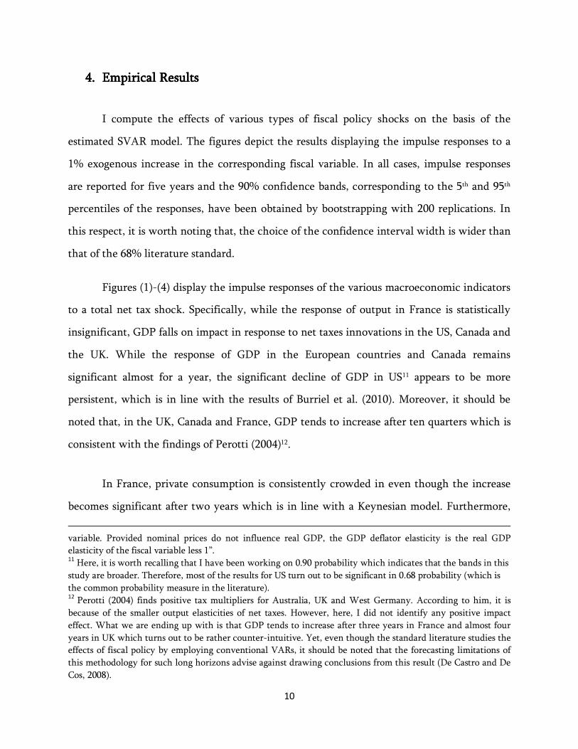
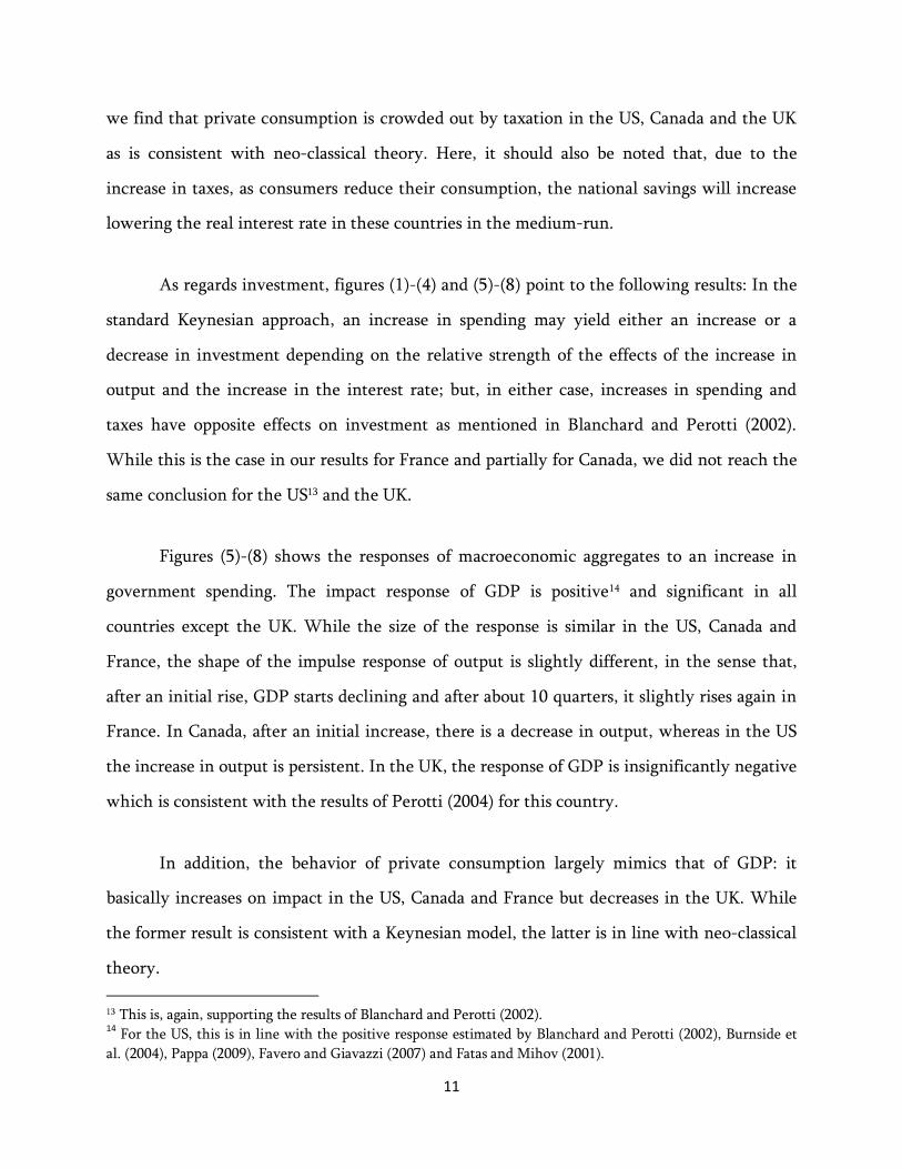
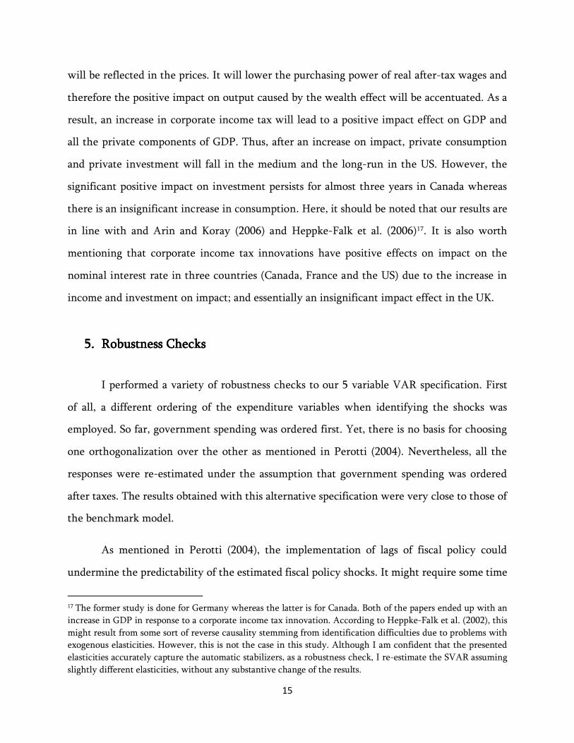
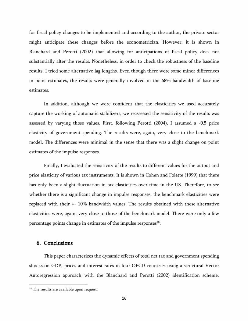
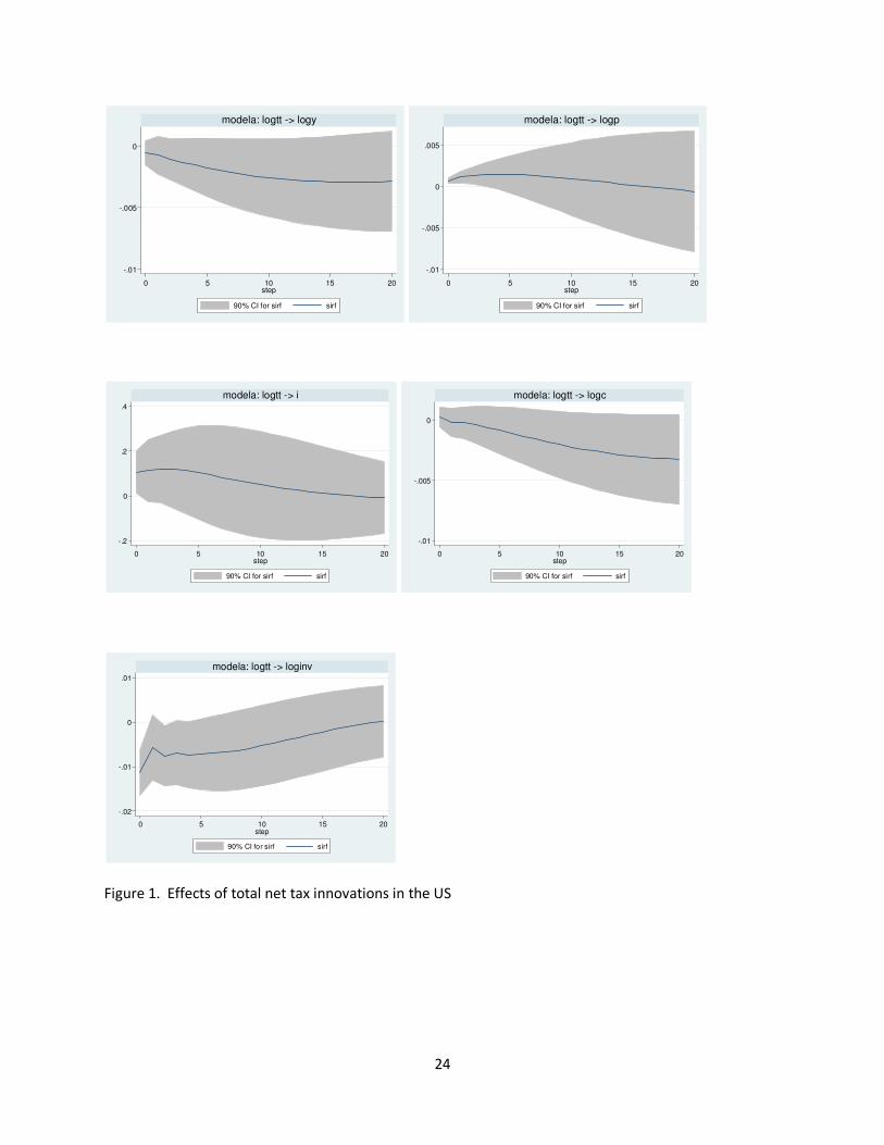
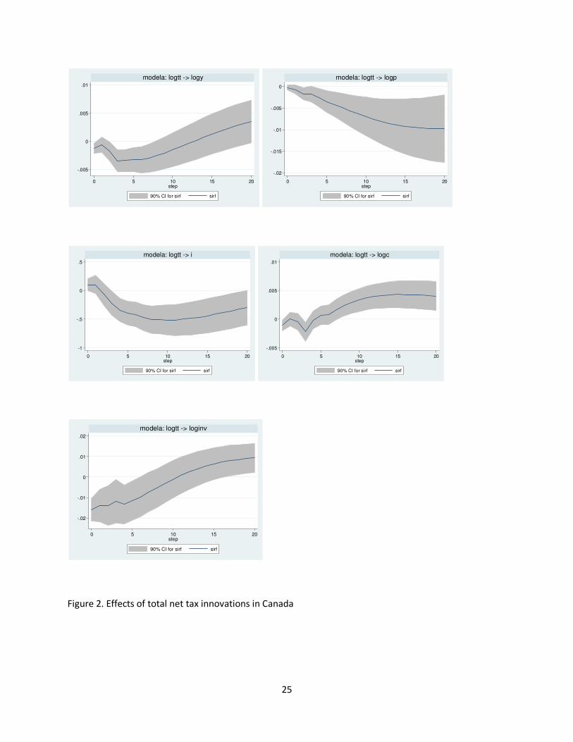
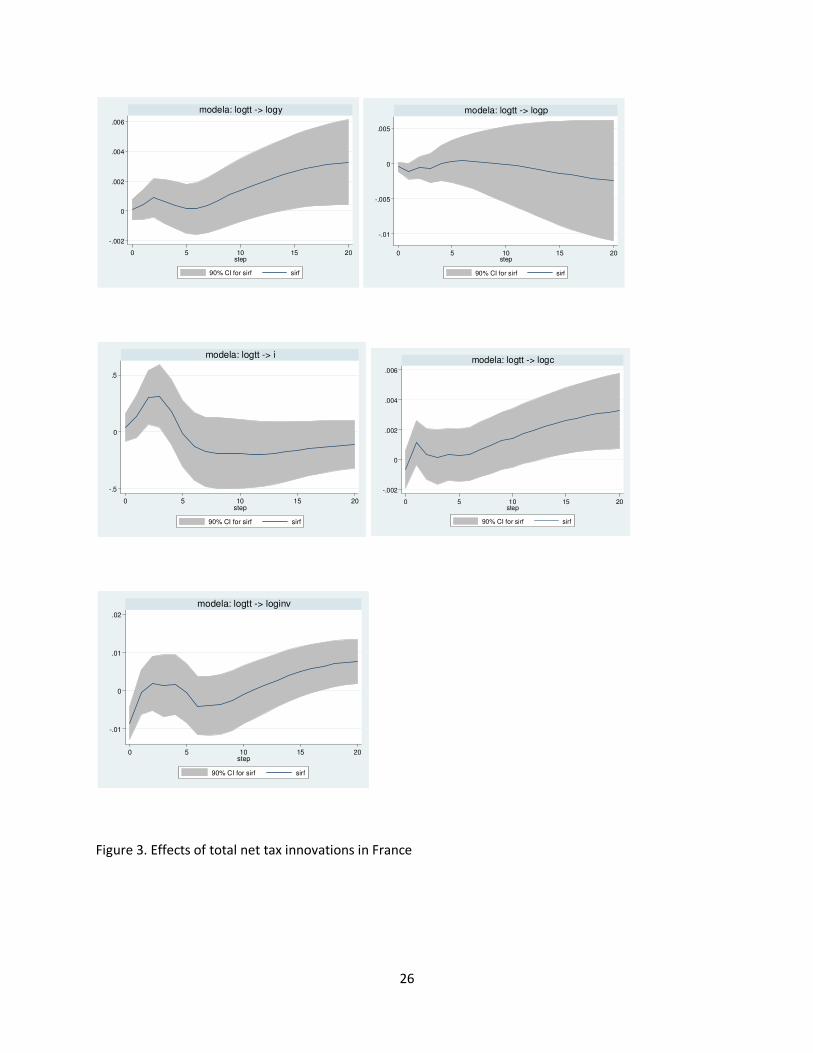
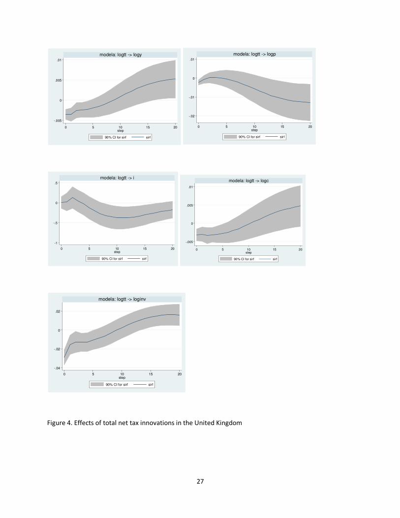
Figures (1)-(4) display the impulse responses of the various macroeconomic indicators

to a total net tax shock. Specifically, while the response of output in France is statistically

insignificant, GDP falls on impact in response to net taxes innovations in the US, Canada and

the UK. While the response of GDP in the European countries and Canada remains

significant almost for a year, the significant decline of GDP in US11 appears to be more

persistent, which is in line with the results of Burriel et al. (2010). Moreover, it should be

noted that, in the UK, Canada and France, GDP tends to increase after ten quarters which is

consistent with the findings of Perotti (2004)12.

In France, private consumption is consistently crowded in even though the increase

becomes significant after two years which is in line with a Keynesian model. Furthermore,

variable. Provided nominal prices do not influence real GDP, the GDP deflator elasticity is the real GDP

elasticity of the fiscal variable less 1”. 11

Here, it is worth recalling that I have been working on 0.90 probability which indicates that the bands in this

study are broader. Therefore, most of the results for US turn out to be significant in 0.68 probability (which is

the common probability measure in the literature). 12 Perotti (2004) finds positive tax multipliers for Australia, UK and West Germany. According to him, it is

because of the smaller output elasticities of net taxes. However, here, I did not identify any positive impact

effect. What we are ending up with is that GDP tends to increase after three years in France and almost four

years in UK which turns out to be rather counter-intuitive. Yet, even though the standard literature studies the

effects of fiscal policy by employing conventional VARs, it should be noted that the forecasting limitations of

this methodology for such long horizons advise against drawing conclusions from this result (De Castro and De

Cos, 2008).

11

we find that private consumption is crowded out by taxation in the US, Canada and the UK

as is consistent with neo-classical theory. Here, it should also be noted that, due to the

increase in taxes, as consumers reduce their consumption, the national savings will increase

lowering the real interest rate in these countries in the medium-run.

As regards investment, figures (1)-(4) and (5)-(8) point to the following results: In the

standard Keynesian approach, an increase in spending may yield either an increase or a

decrease in investment depending on the relative strength of the effects of the increase in

output and the increase in the interest rate; but, in either case, increases in spending and

taxes have opposite effects on investment as mentioned in Blanchard and Perotti (2002).

While this is the case in our results for France and partially for Canada, we did not reach the

same conclusion for the US13 and the UK.

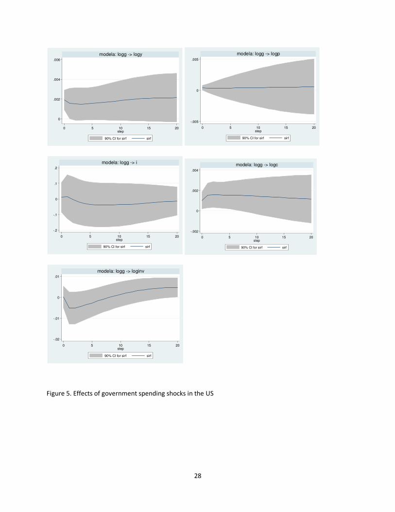
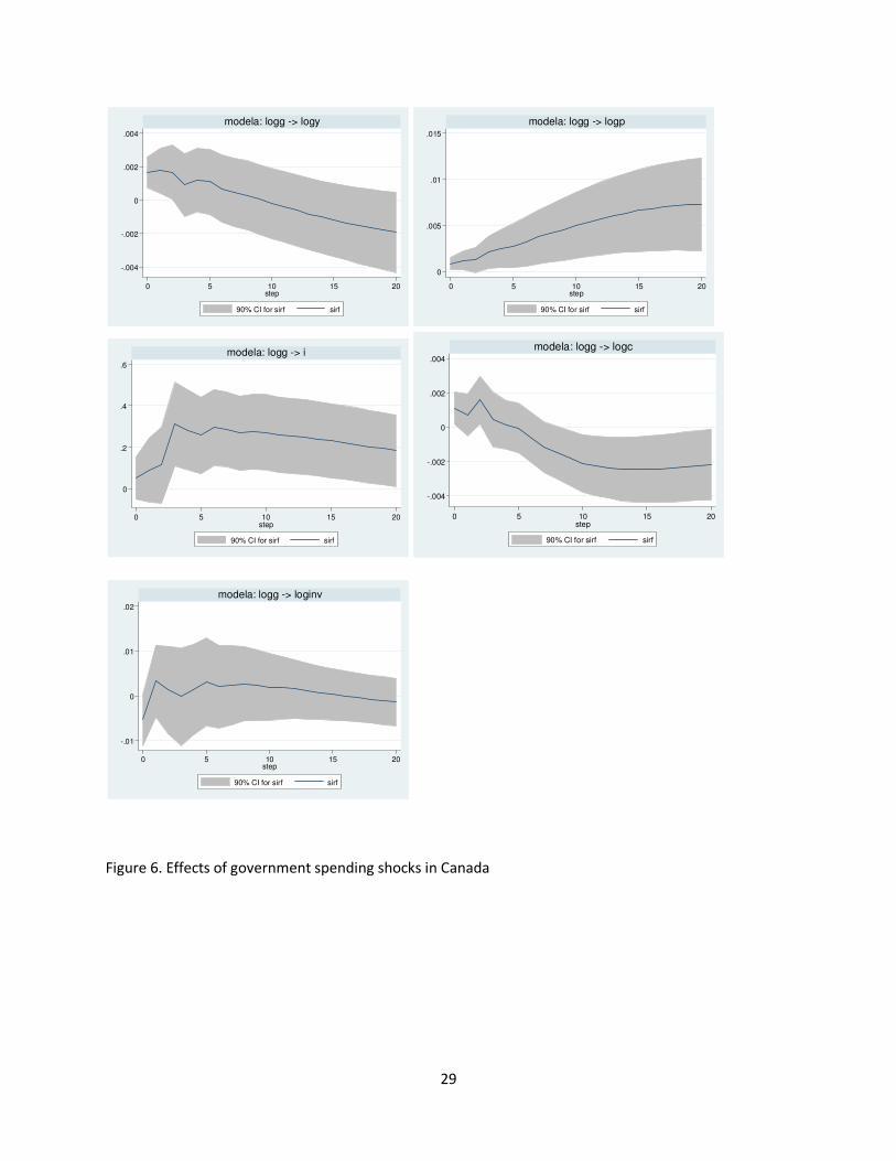
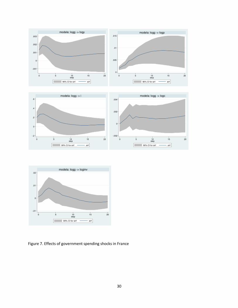
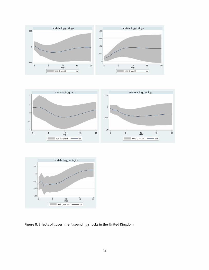
Figures (5)-(8) shows the responses of macroeconomic aggregates to an increase in

government spending. The impact response of GDP is positive14 and significant in all

countries except the UK. While the size of the response is similar in the US, Canada and

France, the shape of the impulse response of output is slightly different, in the sense that,

after an initial rise, GDP starts declining and after about 10 quarters, it slightly rises again in

France. In Canada, after an initial increase, there is a decrease in output, whereas in the US

the increase in output is persistent. In the UK, the response of GDP is insignificantly negative

which is consistent with the results of Perotti (2004) for this country.

In addition, the behavior of private consumption largely mimics that of GDP: it

basically increases on impact in the US, Canada and France but decreases in the UK. While

the former result is consistent with a Keynesian model, the latter is in line with neo-classical

theory.

13 This is, again, supporting the results of Blanchard and Perotti (2002). 14

For the US, this is in line with the positive response estimated by Blanchard and Perotti (2002), Burnside et

al. (2004), Pappa (2009), Favero and Giavazzi (2007) and Fatas and Mihov (2001).

12

Government spending shocks have positive effects on the interest rate in three

countries (Canada, France and the UK) and essentially no impact effect in the US15. It is

useful to note here that, the former result can be reconciled both with a neo-classical and a

Keynesian model.

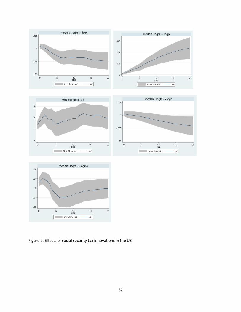
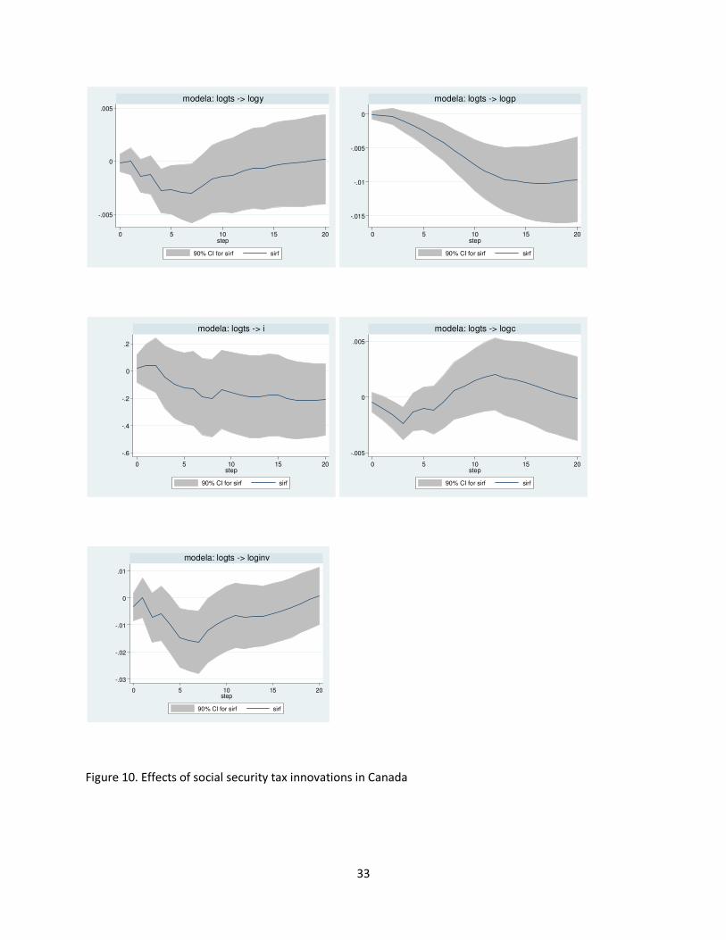
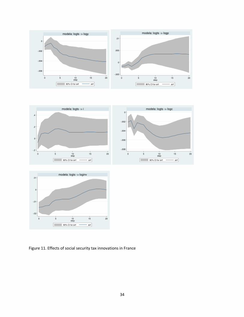
Figures (9)-(12) present the effects of a shock to social security contributions on

macroeconomic indicators. As is widely known, social security taxes are levied on labor as a

payroll tax. A priori, the impact response of output will, therefore, depend on two effects: the

substitution effect and the income effect.

Social security tax innovations will lead to a decrease in tax-payer’s after tax reward

for each extra hour worked, lowering the cost of leisure. Thus, the individual will be willing

to work less in response to lower reward. This is the substitution effect (SE). On the other

hand, a decrease in the real wage will reduce household lifetime earnings and, thus, human

wealth. So, they will not be able to afford additional leisure and, as a result, will supply more

labor. This is the income effect (IE). The relative magnitude of the two effects depends on

the circumstances such as the elasticities of labor supply and demand. Hence, the hours

worked may increase, decrease or remain the same after the tax innovation.

It is seen from figure (9) that in the US, IE dominates SE yielding a significant

increase in output on impact. It is also worth noting that the behavior of private investment

and private consumption mimic that of GDP: it typically increases on impact in this country.

For Canada, France and the UK, higher social security taxes decline output, which decreases

significantly and remains significant for five years in France. As far as GDP components are

concerned, investment and private consumption responses, in general, mimic the GDP’s one.

Some slight differences may be observed though, particularly in the short-run behavior. The

15 Note that the interest rate response in the US and UK are insignificant for the entire period.

13

price level in Canada decreases significantly after four quarters and remains significant for

five years due to the decrease in demand in response to a social security tax innovation in

this country. However, the opposite behavior is observed in France in the sense that, after a

significant decline in the short-run, prices insignificantly rise in the medium-run due to the

0.4 % decrease in output in response to a shock to social security contributions.

The impact effect of the social security tax innovation on the interest rate is positive

in the US due to the increase in money demand and private investment, whereas the

estimated impact effect on the interest rate is insignificant for the rest of the countries.

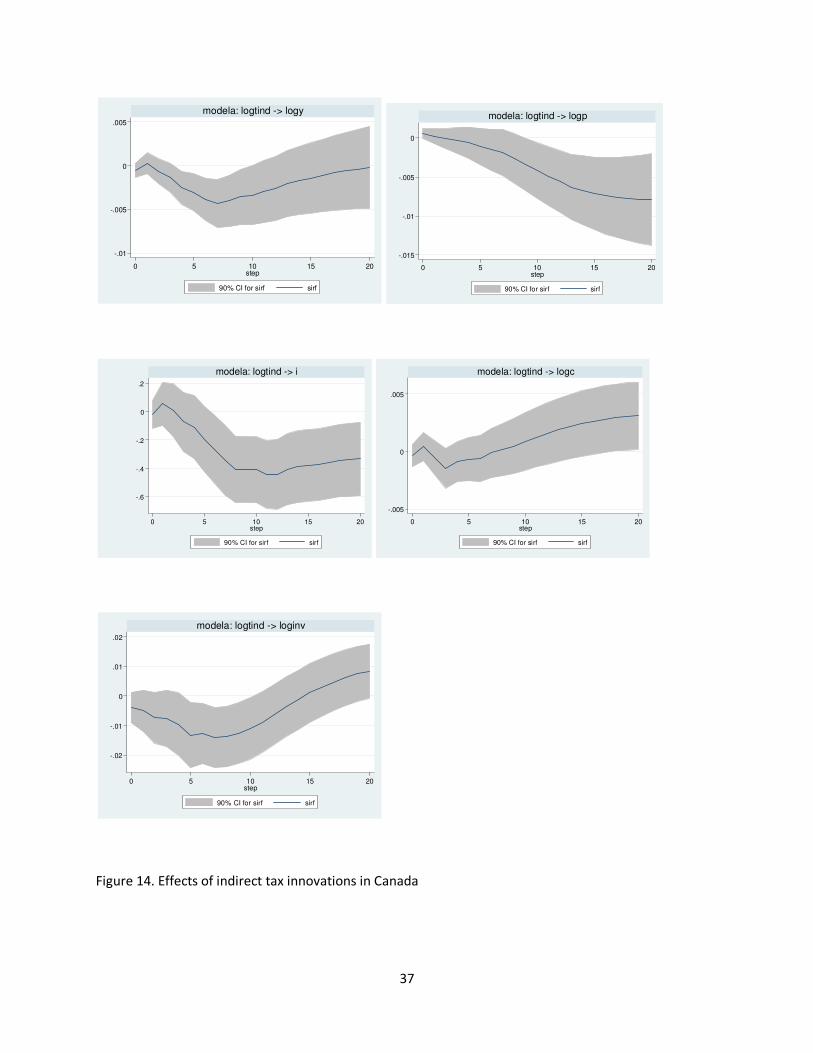
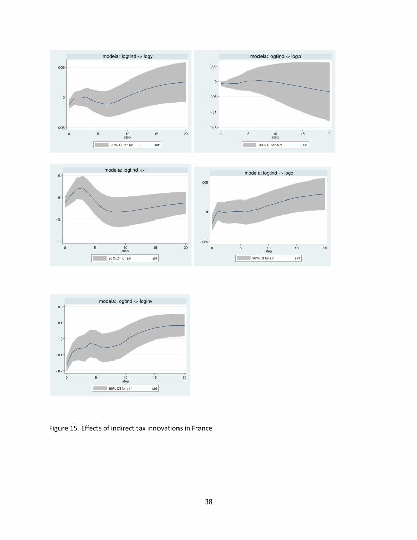
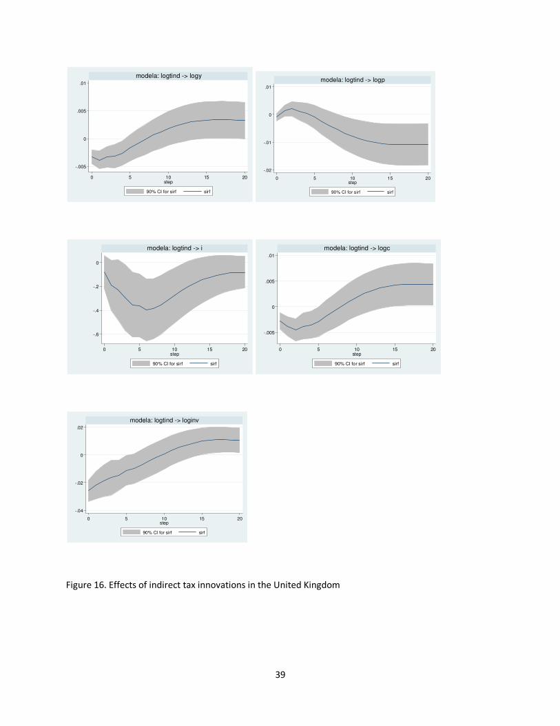
Figures (13)-(16) present the effects of a shock to indirect taxes on macroeconomic

indicators. The response of each component is typically similar across countries, hence

summarizing their shapes is not difficult. Over the whole sample, the impact response is

negative for GDP in all countries. Because they lower the purchasing power of real after-tax

wages, indirect taxes lead to a strong incentive to curtail investment as seen in figures. On

the other hand, since the indirect taxes can be defined as the sales taxes, taxes on goods and

services, there is a decrease in consumption in response to an increase in tax levels. Indirect

tax innovations also lead to a decrease in the price level due to lower demand. Note that,

with the partial exception of Canada and France (where we have seen an insignificant

increase in the interest rate for three quarters), there is a decline in the interest rate on

impact in response to an indirect tax innovation. This can be explained by the decrease in

income and investment levels.

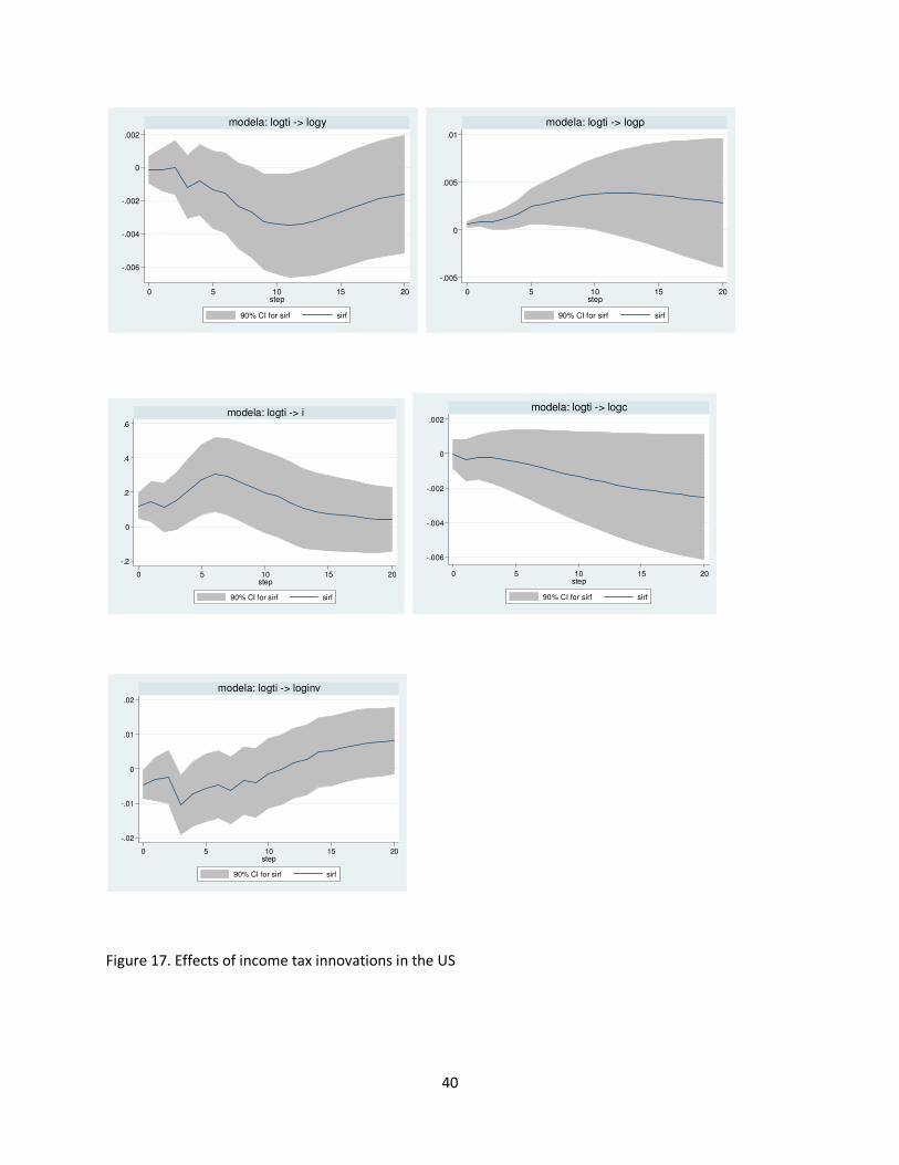
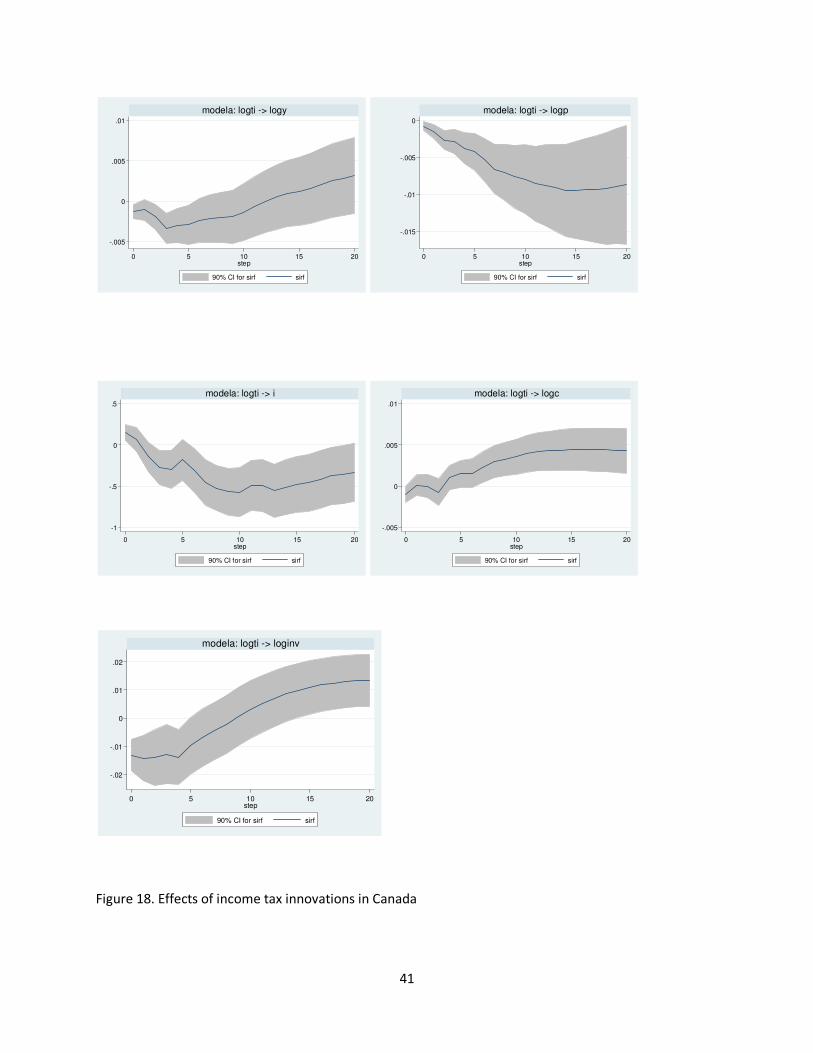
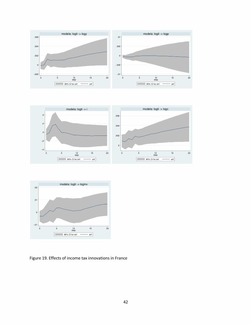
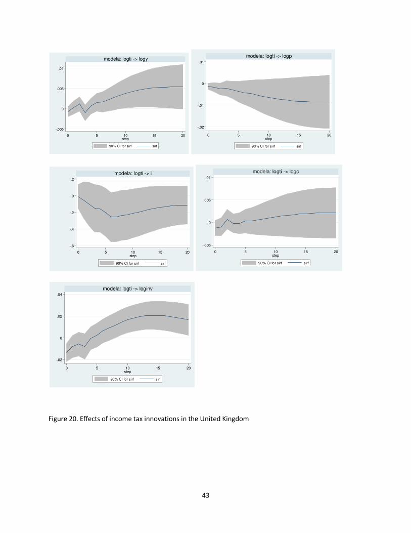
Figures (17)-(20) depict the responses of the endogenous variables to an income tax

innovation. Here, two opposing effects need to be taken into account. First, an increase in

income taxes reduces the household wealth by increasing the present value of household tax

liabilities. Thus, consumption decreases while saving, interest rate and labor supply increases.

However, the rise in hours worked will lead to a decline in real wages, therefore, investment

14

and output increase. This is the wealth effect. Second, the same policy will slow down

economic activity by decreasing output. Because the money demand depends on income, the

decline in output decreases the interest rate which partially crowds in private investment.

The degree of crowding in will hinge on the sensitivity of private investment to income and

the interest rate. Yet, the final effect of the contraction will be a decline in consumption,

investment and output. This is the output effect. Hence, the overall effect on macroeconomic

indicators will depend on these two effects.

For the US, Canada and the UK, the output effect dominates the wealth effect and

therefore the impact response of consumption, investment and output are negative. For

France, although the impact response of output and investment are negative, the output

persistently increases, and there is an insignificant increase in investment after the third

quarter. On the other hand, it should be noted that consumption significantly rises in Canada

and France. There are several ways to explain this16. For instance, Linnemann (2006) applies

a non-seperable utility function in consumption and leisure in a RBC setup in which

consumption and leisure are substitutes. The negative wealth effect of the fiscal contraction

raises hours worked which decreases leisure. The marginal utility of consumption, therefore,

increases. In order to lessen the negative wealth effect, individuals are willing to work more

and to consume more which will lead to an increase in consumption.

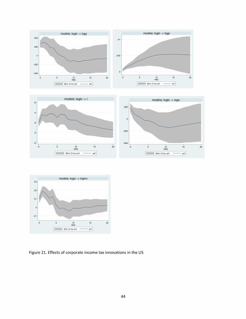
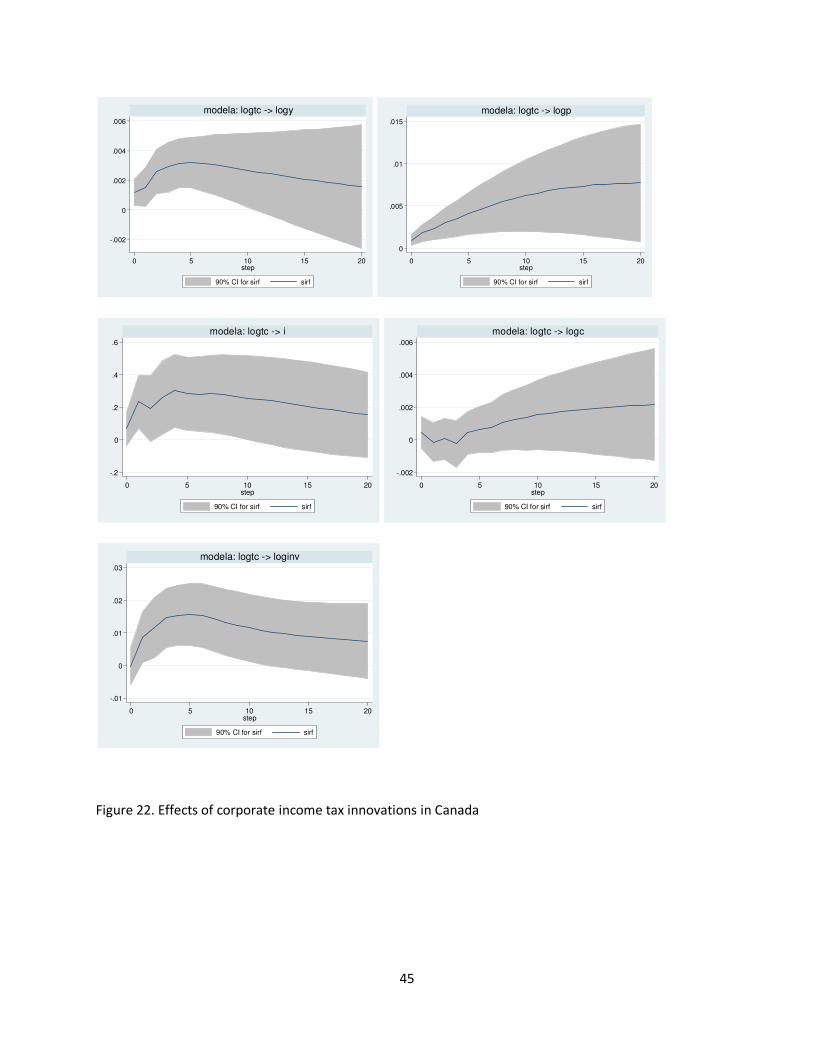
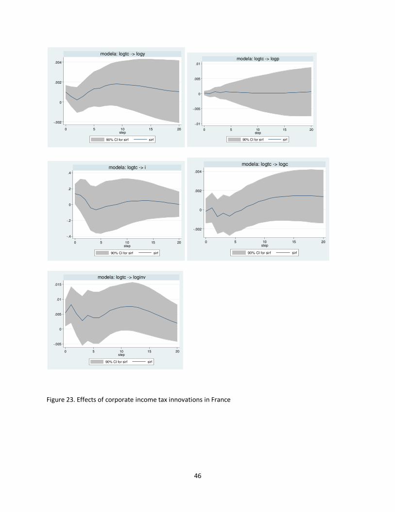
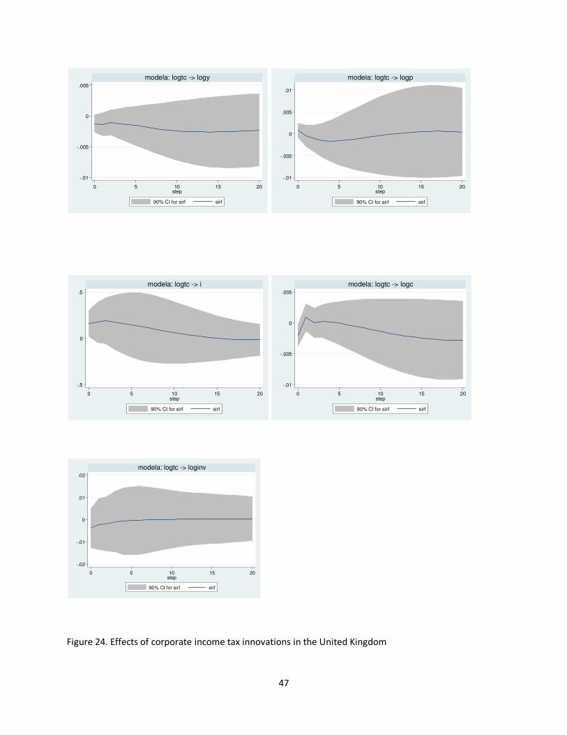
Figures (21)-(24) display the responses of the macroeconomic indicators to a corporate

income tax innovation. The impulse responses show a significant positive response of GDP

on impact for all countries except UK. This can, again, be explained by the negative wealth

effect and output effect. Here, the wealth effect dominates the income effect for Canada,

France and US. Moreover, it should be further noted that the increase in capital income tax

16

Another plausible explanation takes place when habit formation is included in any model. For more details,

see Ravn, Schmitt-Grohe and Uribe (2006), Bouakez and Rebei (2007). Alternatively, Corsetti, Meier and

Muller (2009) modeled a spending reversal effect and ended up with the same conclusion.

15

will be reflected in the prices. It will lower the purchasing power of real after-tax wages and

therefore the positive impact on output caused by the wealth effect will be accentuated. As a

result, an increase in corporate income tax will lead to a positive impact effect on GDP and

all the private components of GDP. Thus, after an increase on impact, private consumption

and private investment will fall in the medium and the long-run in the US. However, the

significant positive impact on investment persists for almost three years in Canada whereas

there is an insignificant increase in consumption. Here, it should be noted that our results are

in line with and Arin and Koray (2006) and Heppke-Falk et al. (2006)17. It is also worth

mentioning that corporate income tax innovations have positive effects on impact on the

nominal interest rate in three countries (Canada, France and the US) due to the increase in

income and investment on impact; and essentially an insignificant impact effect in the UK.

5.5.5.5. Robustness ChecksRobustness ChecksRobustness ChecksRobustness Checks

I performed a variety of robustness checks to our 5 variable VAR specification. First

of all, a different ordering of the expenditure variables when identifying the shocks was

employed. So far, government spending was ordered first. Yet, there is no basis for choosing

one orthogonalization over the other as mentioned in Perotti (2004). Nevertheless, all the

responses were re-estimated under the assumption that government spending was ordered

after taxes. The results obtained with this alternative specification were very close to those of

the benchmark model.

As mentioned in Perotti (2004), the implementation of lags of fiscal policy could

undermine the predictability of the estimated fiscal policy shocks. It might require some time

17 The former study is done for Germany whereas the latter is for Canada. Both of the papers ended up with an

increase in GDP in response to a corporate income tax innovation. According to Heppke-Falk et al. (2002), this

might result from some sort of reverse causality stemming from identification difficulties due to problems with

exogenous elasticities. However, this is not the case in this study. Although I am confident that the presented

elasticities accurately capture the automatic stabilizers, as a robustness check, I re-estimate the SVAR assuming

slightly different elasticities, without any substantive change of the results.

16

for fiscal policy changes to be implemented and according to the author, the private sector

might anticipate these changes before the econometrician. However, it is shown in

Blanchard and Perotti (2002) that allowing for anticipations of fiscal policy does not

substantially alter the results. Nonetheless, in order to check the robustness of the baseline

results, I tried some alternative lag lengths. Even though there were some minor differences

in point estimates, the results were generally involved in the 68% bandwidth of baseline

estimates.

In addition, although we were confident that the elasticities we used accurately

capture the working of automatic stabilizers, we reassessed the sensitivity of the results was

assessed by varying those values. First, following Perotti (2004), I assumed a -0.5 price

elasticity of government spending. The results were, again, very close to the benchmark

model. The differences were minimal in the sense that there was a slight change on point

estimates of the impulse responses.

Finally, I evaluated the sensitivity of the results to different values for the output and

price elasticity of various tax instruments. It is shown in Cohen and Folette (1999) that there

has only been a slight fluctuation in tax elasticities over time in the US. Therefore, to see

whether there is a significant change in impulse responses, the benchmark elasticities were

replaced with their +- 10% bandwidth values. The results obtained with these alternative

elasticities were, again, very close to those of the benchmark model. There were only a few

percentage points change in estimates of the impulse responses18.

6.6.6.6. ConclusionsConclusionsConclusionsConclusions

This paper characterizes the dynamic effects of total net tax and government spending

shocks on GDP, prices and interest rates in four OECD countries using a structural Vector

Autoregression approach with the Blanchard and Perotti (2002) identification scheme.

18 The results are available upon request.

17

Moreover, we propose a structural decomposition of net taxes into four components:

corporate income taxes, income taxes, indirect taxes and social insurance taxes. Our results

suggest that analyzing the fiscal policy by decomposing net taxes and examining their effect

on the aggregate economy provide a more accurate picture than treating net taxes as the

fiscal policy variable.

The main conclusions of the analysis can be summarized as follows: 1)

Decompositions of total net tax innovations show that net tax components are found to have

different impacts on economic variables; 2) The size and persistence of these effects vary

across countries depending on different effects (i.e. negative wealth and output effects,

substitution effect and income effect) resulting from the structure of these economies; 3) The

positive tax multipliers reported in previous studies are found only for corporate income tax

in the US, Canada and France and for social security tax in the US; 4) As regards macro

theories, on the one hand, we find that private investment is crowded out both by taxation

and government spending in the UK and the US as is consistent with the neo-classical model.

On the other hand, our results for France and partially for Canada indicate that there are

opposite effects of tax and spending increases on private investment that are in line with

Keynesian theory; 5) Private consumption is crowded in by government spending for all

countries except the UK, and crowded out by taxation in all countries except France. While

the former result is consistent with a Keynesian model, the latter is in line with neo-classical

theory.

My analysis sheds light on the interpretation of positive net tax multipliers found in

the existing literature. Decompositions of net tax innovations will help us better assess the

macroeconomic implications of fiscal policy shocks and, it is, therefore, important that we

understand the extent to which increases in net taxes are driven by one shock or another.

18

The findings in this paper also indicate that existing approaches to modeling fiscal

policy shocks have to be re-thought. First, the results suggest that the usefulness of the

existing macroeconomic applied work built on the assumption of “total” tax changes may be

unclear. In examining the transmission mechanism of fiscal policy shocks, it is seen from our

results that the traditional priority on net tax shocks may be misleading. Instead, more

attention needs to be paid to different tax policy instruments.

19

References:References:References:References:

Alesina, A., Ardagna, S., Perotti, R., Schiantarelli, F., 2002. Fiscal Policy, Profits and

Investment. American Economic Review, 92(3): 571-589.

Arin, P. K. and Koray, F. 2006. Are some taxes different than others? An empirical

investigation of the effects of tax policy in Canada. Empirical Economics 31: 183-193.

Barro, R., 1990. Government Spending in a Simple Model of Endogenous Growth.

Journal of Political Economy 98(1): 103-117.

Baxter, M., King, R. G., 1993. Fiscal Policy in General Equilibrium. American

Economic Review, American Economic Association, vol. 83(3): 315-34.

Blanchard, O., Perotti R., 2002. An Empirical Characterization of the Dynamic Effects

of Changes in Government Spending and Taxes on Output. Quarterly Journal of Economics

177: 1329-1368.

Bouakez, H. and Rebei, N. 2007. Why does private consumption rise after a

government spending shock?. Canadian Journal of Economics 40: 954-79.

Burnside, C., Eichenbaum, M. and Fisher, J. 2004. Fiscal shocks and their

consequences. Journal of Economic Theory, 115: 89-117.

Burriel, P., De Castro, F., Garrote, D., Gordo, E., Paredes, J., Perez, J. 2010. Fiscal

Policy Shocks in the Euro Area and the US: An Empirical Assessment. Fiscal Studies, 31(2):

251-285.

Cohen, D., Folette, G. 1999. The Automatic Fiscal Stabilizers: Quietly Doing Their

Thing. Division of Research and Statistics, Federal Reserve Board.

Corsetti, G., Meier, A. and Müller, G. 2010. Cross-border spillovers from fiscal

stimulus. International Journal of Central Banking 6: 5-37.

20

Daude, C., Melguizo, A., Neut, A. 2010. Fiscal Policy in Latin America: Counter-

cyclical and Sustainable at last? OECD Development Centre, Working Paper No: 291.

De Castro, F. and de Cos, P. 2008. The economic effects of fiscal policy: the case of

Spain. Journal of Macroeconomics 30: 1005-1028.

Fatás, A. and Mihov, I. 2001. The effects of fiscal policy on consumption and

employment: theoryand evidence. CEPR Discussion 2760.

Favero, C. and Giavazzi, F. 2007. Debt and the effect of fiscal policy. NBER Working

Paper 12822.

Giordano, R., Momigliano, S. Neri, S., and Perotti, R. 2007. The effects of fiscal policy

in Italy: estimates from a VAR model. European Journal of Political Economy 23: 707-733.

Gordon, R. H., Kalambokidis, L., Rohaly, J. & Slemrod, J. 2004. Toward a

consumption tax, and beyond. American Economic Review, Papers and Proceedings 94(2):

161-165.

Gordon, R. H., Kalambokidis, L. & Slemrod, J. 2004a. If capital income taxes are so

high, why do we collect so little revenue? A new summary measure of the effective tax rates

on investment, in P. B. Sorensen (ed.), Measuring the Tax Burden on Capital and Labour,

MIT Press, Cambridge, USA, chapter 4.

Hemming, R., Kell, M. and Mahfouz, S. 2002. The effectiveness of fiscal policy in

stimulating economic activity- a review of the literature. International Monetary Fund

Working Paper 02/208.

Heppke-Falk, K., Tenhofen, J., and Wolff, G. 2006. The macroeconomic effects of

exogenous fiscal policy shocks in Germany: a disaggregated analysis. Deutsche Bundesbank

Discussion Paper 41.

Kim, S. and Roubini, N. 2008. Twin deficit or twin divergence? Fiscal policy, current

account, and real exchange rate in the U.S. Journal of International Economics 74: 362-83.

21

Linnemann, L. 2006. The effects of government spending on private consumption: a

puzzle? Journal of Money, Credit and Banking 38: 1715-35.

Lutkepohl, H. 1991. Introduction to Multiple Time Series Analysis. Springer-Verlag,

Berlin.

Mertens, K. and Ravn, M. 2009. Understanding the aggregate effects of anticipated

and unanticipated tax policy shocks. EUI, mimeo.

Monacelli, T. and Perotti, R. 2010. Fiscal policy, the real exchange rate, and traded

goods. Economic Journal 120: 437-461.

Mounford, A., Uhlig, H., 2008. What are the Effects of Fiscal Policy Shocks? NBER

Working Paper Series 14551.

Pappa, E. 2009. The effects of fiscal shocks on employment and real wages.

International Economic Review 50: 217-44.

Perotti, R., 2004. Estimating the Effects of Fiscal Policy in OECD Countries. CEPR

Working Paper n. 276.

Perotti, R. 2007. In search of the transmission mechanism of fiscal policy. NBER

Macroeconomic Manual 2007 22.

Ramey, A. 2008. Identifying government spending shocks: it’s all in the timing.

UCSD, mimeo.

Ravn, M., Schmitt-Grohé, S. and Uribe, M. 2006. Deep habits. Review of Economic

Studies 73: 195-218.

Romer, C. and Romer, D. 2010. The macroeconomic effects of tax changes: estimates

based on a new measure of fiscal shocks. American Economic Review 100: 763–801.

Tenhofen, J. and Wolff, G. 2007. Does anticipation of government spending matter?

Evidence from an expectation augmented VAR. Deutsche Bundesbank Discussion Paper 14.

22

Van den Noord, P. 2000. “The Size and Role of Automatic Fiscal Stabilizers in the

1990s and Beyond”, OECD Economics Department Working Papers, No. 230.

23

Appendix:Appendix:Appendix:Appendix:

Table 1. Exogenous Elasticities

United StatesUnited StatesUnited StatesUnited States CanadaCanadaCanadaCanada FranceFranceFranceFrance United KingdomUnited KingdomUnited KingdomUnited Kingdom

,-./ 1.8 1 1.8 0.6

,-.0 0.6 1.2 0.6 1.4

,-.1 0.6 0.9 0.5 1.2

,-.023 0.9 0.7 0.7 1.1

,-4 1.1 1 1 1.1

,-5 0 0 0 0

,6./ 0.8 0 0.8 -0.4

,6.0 -0.4 0.2 -0.4 0.4

,6.1 -0.4 -0.1 -0.5 0.2

,6.023 -0.4 -0.3 -0.3 0.1

,64 -0.1 0 0 0.1

,65 -1 -1 -1 -1

,/./ 1.44 0.75 1.35 0.48

,/.0 0.48 0.9 0.45 1.12

,/.1 0.48 0.675 0.975 0.96

,/.023 0.72 0.525 0.525 0.88

,/4 0.88 0.75 0.75 0.88

,/5 0 0 0 0

,027./ 0.36 0.25 0.45 0.12

,027.0 0.12 0.3 0.15 0.28

,027.1 0.12 0.225 0.125 0.24

,027.023 0.18 0.175 0.175 0.22

,0274 0.22 0.25 0.25 0.22

,0275 0 0 0 0

�: total net tax

89: corporate income tax

8 : income tax

8 :;: indirect tax

8<: social security tax

$=>: private investment

c: private consumption

�: government spending (public consumption + public investment)

24

Figure 1. Effects of total net tax innovations in the US

-.01

-.005

0

0 5 10 15 20step

90% CI for sirf sirf

modela: logtt -> logy

-.01

-.005

0

.005

0 5 10 15 20step


modela: logtt -> logp

-.2

0

.2

.4

0 5 10 15 20step


modela: logtt -> i

-.01

-.005

0

0 5 10 15 20step


modela: logtt -> logc

-.02

-.01

0

.01

0 5 10 15 20step


modela: logtt -> loginv

25

Figure 2. Effects of total net tax innovations in Canada

-.005

0

.005

.01

0 5 10 15 20step



-.02

-.015

-.01

-.005

0

0 5 10 15 20step



-1

-.5

0

.5

0 5 10 15 20step


modela: logtt -> i

-.005

0

.005

.01

0 5 10 15 20step



-.02

-.01

0

.01

.02

0 5 10 15 20step



26

Figure 3. Effects of total net tax innovations in France

-.002

0

.002

.004

.006

0 5 10 15 20step



-.01

-.005

0

.005

0 5 10 15 20step



-.5

0

.5

0 5 10 15 20step


modela: logtt -> i

-.002

0

.002

.004

.006

0 5 10 15 20step



-.01

0

.01

.02

0 5 10 15 20step



27

Figure 4. Effects of total net tax innovations in the United Kingdom

-.005

0

.005

.01

0 5 10 15 20step



-.02

-.01

0

.01

0 5 10 15 20step



-1

-.5

0

.5

0 5 10 15 20step


modela: logtt -> i

-.005

0

.005

.01

0 5 10 15 20step



-.04

-.02

0

.02

0 5 10 15 20step



28

Figure 5. Effects of government spending shocks in the US

0

.002

.004

.006

0 5 10 15 20step


modela: logg -> logy

-.005

0

.005

0 5 10 15 20step


modela: logg -> logp

-.2

-.1

0

.1

.2

0 5 10 15 20step


modela: logg -> i

-.002

0

.002

.004

0 5 10 15 20step


modela: logg -> logc

-.02

-.01

0

.01

0 5 10 15 20step


modela: logg -> loginv

29

Figure 6. Effects of government spending shocks in Canada

-.004

-.002

0

.002

.004

0 5 10 15 20step



0

.005

.01

.015

0 5 10 15 20step



0

.2

.4

.6

0 5 10 15 20step


modela: logg -> i

-.004

-.002

0

.002

.004

0 5 10 15 20step



-.01

0

.01

.02

0 5 10 15 20step



30

Figure 7. Effects of government spending shocks in France

-.001

0

.001

.002

.003

0 5 10 15 20step



0

.005

.01

.015

0 5 10 15 20step



-.2

0

.2

.4

.6

0 5 10 15 20step


modela: logg -> i

-.002

0

.002

.004

0 5 10 15 20step



-.01

0

.01

.02

0 5 10 15 20step



31

Figure 8. Effects of government spending shocks in the United Kingdom

-.005

0

.005

0 5 10 15 20step



0

.005

.01

.015

.02

0 5 10 15 20step



-.4

-.2

0

.2

.4

0 5 10 15 20step


modela: logg -> i

-.01

-.005

0

.005

0 5 10 15 20step



-.03

-.02

-.01

0

.01

0 5 10 15 20step



32

Figure 9. Effects of social security tax innovations in the US

-.01

-.005

0

.005

0 5 10 15 20step


modela: logts -> logy

0

.005

.01

.015

0 5 10 15 20step


modela: logts -> logp

-.2

0

.2

.4

0 5 10 15 20step


modela: logts -> i

-.01

-.005

0

.005

0 5 10 15 20step


modela: logts -> logc

-.02

-.01

0

.01

.02

0 5 10 15 20step


modela: logts -> loginv

33

Figure 10. Effects of social security tax innovations in Canada

-.005

0

.005

0 5 10 15 20step



-.015

-.01

-.005

0

0 5 10 15 20step



-.6

-.4

-.2

0

.2

0 5 10 15 20step


modela: logts -> i

-.005

0

.005

0 5 10 15 20step



-.03

-.02

-.01

0

.01

0 5 10 15 20step



34

Figure 11. Effects of social security tax innovations in France

-.006

-.004

-.002

0

0 5 10 15 20step



-.005

0

.005

.01

0 5 10 15 20step



-.2

0

.2

.4

0 5 10 15 20step


modela: logts -> i

-.008

-.006

-.004

-.002

0

0 5 10 15 20step



-.02

-.01

0

.01

0 5 10 15 20step



35

Figure 12. Effects of social security tax innovations in the United Kingdom

-.005

0

.005

.01

0 5 10 15 20step



-.01

0

.01

.02

0 5 10 15 20step



-.4

-.2

0

.2

.4

0 5 10 15 20step


modela: logts -> i

-.005

0

.005

.01

0 5 10 15 20step



-.04

-.02

0

.02

.04

0 5 10 15 20step



36

Figure 13. Effects of indirect tax innovations in the US

-.005

0

.005

0 5 10 15 20step


modela: logtind -> logy

-.015

-.01

-.005

0

0 5 10 15 20step


modela: logtind -> logp

-.6

-.4

-.2

0

.2

0 5 10 15 20step


modela: logtind -> i

-.005

0

.005

0 5 10 15 20step


modela: logtind -> logc

-.02

-.01

0

.01

0 5 10 15 20step


modela: logtind -> loginv

37

Figure 14. Effects of indirect tax innovations in Canada

-.01

-.005

0

.005

0 5 10 15 20step



-.015

-.01

-.005

0

0 5 10 15 20step



-.6

-.4

-.2

0

.2

0 5 10 15 20step



-.005

0

.005

0 5 10 15 20step



-.02

-.01

0

.01

.02

0 5 10 15 20step



38

Figure 15. Effects of indirect tax innovations in France

-.005

0

.005

0 5 10 15 20step



-.015

-.01

-.005

0

.005

0 5 10 15 20step



-1

-.5

0

.5

0 5 10 15 20step



-.005

0

.005

0 5 10 15 20step



-.02

-.01

0

.01

.02

0 5 10 15 20step



39

Figure 16. Effects of indirect tax innovations in the United Kingdom

-.005

0

.005

.01

0 5 10 15 20step



-.02

-.01

0

.01

0 5 10 15 20step



-.6

-.4

-.2

0

0 5 10 15 20step



-.005

0

.005

.01

0 5 10 15 20step



-.04

-.02

0

.02

0 5 10 15 20step



40

Figure 17. Effects of income tax innovations in the US

-.006

-.004

-.002

0

.002

0 5 10 15 20step


modela: logti -> logy

-.005

0

.005

.01

0 5 10 15 20step


modela: logti -> logp

-.2

0

.2

.4

.6

0 5 10 15 20step


modela: logti -> i

-.006

-.004

-.002

0

.002

0 5 10 15 20step


modela: logti -> logc

-.02

-.01

0

.01

.02

0 5 10 15 20step


modela: logti -> loginv

41

Figure 18. Effects of income tax innovations in Canada

-.005

0

.005

.01

0 5 10 15 20step



-.015

-.01

-.005

0

0 5 10 15 20step



-1

-.5

0

.5

0 5 10 15 20step


modela: logti -> i

-.005

0

.005

.01

0 5 10 15 20step



-.02

-.01

0

.01

.02

0 5 10 15 20step



42

Figure 19. Effects of income tax innovations in France

-.002

0

.002

.004

.006

0 5 10 15 20step



-.01

-.005

0

.005

.01

0 5 10 15 20step



-.4

-.2

0

.2

.4

0 5 10 15 20step


modela: logti -> i

0

.002

.004

.006

0 5 10 15 20step



-.01

0

.01

.02

0 5 10 15 20step



43

Figure 20. Effects of income tax innovations in the United Kingdom

-.005

0

.005

.01

0 5 10 15 20step



-.02

-.01

0

.01

0 5 10 15 20step



-.6

-.4

-.2

0

.2

0 5 10 15 20step


modela: logti -> i

-.005

0

.005

.01

0 5 10 15 20step



-.02

0

.02

.04

0 5 10 15 20step



44

Figure 21. Effects of corporate income tax innovations in the US

-.004

-.002

0

.002

.004

0 5 10 15 20step


modela: logtc -> logy

0

.005

.01

0 5 10 15 20step


modela: logtc -> logp

-.2

0

.2

.4

.6

0 5 10 15 20step


modela: logtc -> i

-.004

-.002

0

.002

0 5 10 15 20step


modela: logtc -> logc

-.01

0

.01

.02

.03

0 5 10 15 20step


modela: logtc -> loginv

45

Figure 22. Effects of corporate income tax innovations in Canada

-.002

0

.002

.004

.006

0 5 10 15 20step



0

.005

.01

.015

0 5 10 15 20step



-.2

0

.2

.4

.6

0 5 10 15 20step


modela: logtc -> i

-.002

0

.002

.004

.006

0 5 10 15 20step



-.01

0

.01

.02

.03

0 5 10 15 20step



46

Figure 23. Effects of corporate income tax innovations in France

-.002

0

.002

.004

0 5 10 15 20step



-.01

-.005

0

.005

.01

0 5 10 15 20step



-.4

-.2

0

.2

.4

0 5 10 15 20step


modela: logtc -> i

-.002

0

.002

.004

0 5 10 15 20step



-.005

0

.005

.01

.015

0 5 10 15 20step



47

Figure 24. Effects of corporate income tax innovations in the United Kingdom

-.01

-.005

0

.005

0 5 10 15 20step



-.01

-.005

0

.005

.01

0 5 10 15 20step



-.5

0

.5

0 5 10 15 20step


modela: logtc -> i

-.01

-.005

0

.005

0 5 10 15 20step



-.02

-.01

0

.01

.02

0 5 10 15 20step



Rethinking the Effects of Fiscal Policy on Macroeconomic

Documents

Transcript of Rethinking the Effects of Fiscal Policy on Macroeconomic