RESOURCE ALLOCATION FORUPLINK CODE-DOMAIN

NON-ORTHOGONAL MULTIPLEACCESS

A THESIS SUBMITTED TO THE UNIVERSITY OF MANCHESTER

FOR THE DEGREE OF DOCTOR OF PHILOSOPHY

IN THE FACULTY OF SCIENCE AND ENGINEERING

2021

Yanely Montserrat Jimenez Licea

Department of Electrical and Electronic Engineering

Contents

List of Tables 6

List of Figures 7

Abstract 10

Declaration 11

Copyright 12

Acknowledgements 13

List of Abbreviations 14

List of Mathematical Notation 17

List of Variables 18

1 Introduction 23

1.1 Motivation . . . . . . . . . . . . . . . . . . . . . . . . . . . . . . . . 27

1.2 Contributions . . . . . . . . . . . . . . . . . . . . . . . . . . . . . . 28

1.3 Thesis organization . . . . . . . . . . . . . . . . . . . . . . . . . . . 29

1.4 Publications . . . . . . . . . . . . . . . . . . . . . . . . . . . . . . . 30

2

2 Non orthogonal multiple access 31

2.1 Introduction . . . . . . . . . . . . . . . . . . . . . . . . . . . . . . . 31

2.2 Wireless channels theory . . . . . . . . . . . . . . . . . . . . . . . . 32

2.2.1 Path loss and shadowing . . . . . . . . . . . . . . . . . . . . 32

2.2.2 Fading and multipath effect . . . . . . . . . . . . . . . . . . 33

2.3 Non orthogonal multiple access in the uplink . . . . . . . . . . . . . 34

2.3.1 Successive Interference Cancellation . . . . . . . . . . . . . . 36

2.3.2 Sum rate and decoding order for NOMA uplink system . . . . 36

2.4 Coded Non-orthogonal Multiple Access . . . . . . . . . . . . . . . . 40

2.5 Chapter summary . . . . . . . . . . . . . . . . . . . . . . . . . . . . 42

3 Sparse Code Multiple Access 43

3.1 SCMA codebook design . . . . . . . . . . . . . . . . . . . . . . . . 44

3.2 SCMA transmission . . . . . . . . . . . . . . . . . . . . . . . . . . . 53

3.3 SCMA receiver and signal detection . . . . . . . . . . . . . . . . . . 55

3.4 Factor graph design and sparsity . . . . . . . . . . . . . . . . . . . . 59

3.5 Sparsity of codewords . . . . . . . . . . . . . . . . . . . . . . . . . . 60

3.6 Numerical results . . . . . . . . . . . . . . . . . . . . . . . . . . . . 60

3.7 Chapter summary . . . . . . . . . . . . . . . . . . . . . . . . . . . . 65

4 Resource allocation for Uplink SCMA System 66

4.1 SCMA capacity and resource allocation . . . . . . . . . . . . . . . . 67

4.2 Subcarrier allocation for SCMA . . . . . . . . . . . . . . . . . . . . 68

4.2.1 Greedy algorithm based methods . . . . . . . . . . . . . . . . 68

4.2.1.1 Proposed subcarrier allocation algorithm . . . . . . 68

4.2.1.2 Low complexity proposed algorithm . . . . . . . . 71

3

4.2.2 Matching Theory . . . . . . . . . . . . . . . . . . . . . . . . 71

4.2.2.1 Considerations of matching theory in SCMA . . . . 75

4.2.2.2 Complexity of Matching theory for SCMA . . . . . 77

4.3 Power allocation solution . . . . . . . . . . . . . . . . . . . . . . . . 78

4.3.1 Problem formulation and solution . . . . . . . . . . . . . . . 78

4.3.2 Problem solution using Lagrange dual solution and subgradi-ent algorithm in SCMA . . . . . . . . . . . . . . . . . . . . . 80

4.4 Numerical results . . . . . . . . . . . . . . . . . . . . . . . . . . . . 83

4.5 Chapter summary . . . . . . . . . . . . . . . . . . . . . . . . . . . . 93

5 Pattern Division Multiple Access uplink system 94

5.1 PDMA transmission . . . . . . . . . . . . . . . . . . . . . . . . . . . 95

5.2 Factor graph design and sparsity in PDMA . . . . . . . . . . . . . . . 96

5.3 PDMA and resource allocation . . . . . . . . . . . . . . . . . . . . . 98

5.3.1 Subcarrier allocation in PDMA . . . . . . . . . . . . . . . . 99

5.3.2 Proposed subcarrier allocation algorithm based on greedy al-gorithm . . . . . . . . . . . . . . . . . . . . . . . . . . . . . 99

5.4 Power allocation in PDMA . . . . . . . . . . . . . . . . . . . . . . . 101

5.4.1 Optimal power allocation for sum rate maximization in PDMAwith power constraint . . . . . . . . . . . . . . . . . . . . . . 103

5.4.2 Problem solution using Lagrange dual solution and subgradi-ent algorithm in PDMA for power allocation with minimumrate constraint . . . . . . . . . . . . . . . . . . . . . . . . . . 107

5.5 Numerical results . . . . . . . . . . . . . . . . . . . . . . . . . . . . 118

5.6 Chapter summary . . . . . . . . . . . . . . . . . . . . . . . . . . . . 123

6 Conclusions and future works 124

6.1 Conclusions . . . . . . . . . . . . . . . . . . . . . . . . . . . . . . . 124

4

6.2 Future works . . . . . . . . . . . . . . . . . . . . . . . . . . . . . . 125

6.2.1 Coded NOMA with multiple antennas . . . . . . . . . . . . . 125

6.2.2 Massive connectivity and resource management . . . . . . . . 126

6.2.3 Cache-aided D2D communication . . . . . . . . . . . . . . . 126

References 127

A Multiplexed signal for SCMA system 138

B Proof 1: Independence of decoding order on uplink sum rate 142

C Proof 2: Derivation of the SINR for the SCMA rate equation 145

D Proof 3: Derivation of the SNR for the SCMA rate equation 147

E Proof 4: Derivation of the rate per section in PDMA 149

F Multiplexed signal for PDMA system 152

5

List of Tables

2.1 ITU Pedestrian Model . . . . . . . . . . . . . . . . . . . . . . . . . . 34

3.1 Parameters of link performance simulation for SCMA and PDMA . . 61

4.1 Parameters of simulation for SCMA . . . . . . . . . . . . . . . . . . 84

4.2 Complexity comparison of subcarrier allocation schemes . . . . . . . 87

5.1 Parameters of simulation for PDMA4X6 . . . . . . . . . . . . . . . . 118

6

List of Figures

1.1 Pyramid deployment of 5G industry . . . . . . . . . . . . . . . . . . 24

1.2 Graphic representation of downlink and uplink . . . . . . . . . . . . 25

2.1 Graphic representation of different multiple access techniques . . . . 35

2.2 Successive Interference Cancellation process . . . . . . . . . . . . . 36

2.3 SCMA uplink transmission . . . . . . . . . . . . . . . . . . . . . . . 38

3.1 Diagram of SCMA system components . . . . . . . . . . . . . . . . 44

3.2 Rotation of vector S1 to obtain the Mother Constellation [60] . . . . . 46

3.3 SCMA system transmission representation . . . . . . . . . . . . . . . 53

3.4 Graphic representation of the codebooks and multiplexed signals . . . 54

3.5 Graph showing the connection of variable nodes with function nodes. 57

3.6 Probability functions diagram . . . . . . . . . . . . . . . . . . . . . . 58

3.7 BER performance of SCMA system in the uplink for the purpose ofcomparison with PDMA . . . . . . . . . . . . . . . . . . . . . . . . 62

3.8 BER performance of SCMA systems in the uplink per user . . . . . . 63

3.9 Comparison of average BER in SCMA vs PDMA systems . . . . . . 64

3.10 BER per user in PDMA system. The users are ordered from low BERto high BER. User 1 shows the lowest BER and user 6 shows the high-est BER. . . . . . . . . . . . . . . . . . . . . . . . . . . . . . . . . . 65

4.1 Graphic representation of first user’s subcarrier allocation . . . . . . . 69

7

4.2 Graphic example of odd and even numbered users’ subcarrier allocation 70

4.3 Swap blocking pairs . . . . . . . . . . . . . . . . . . . . . . . . . . . 74

4.4 Graphic representation of a swap operation . . . . . . . . . . . . . . 74

4.5 Example of a pivot element to start looking for possible blocking pairs 75

4.6 Subcarrier allocation in SCMA . . . . . . . . . . . . . . . . . . . . . 85

4.7 Comparison of total rate of the classic greedy method and our proposedalgorithm for subcarrier allocation in SCMA . . . . . . . . . . . . . . 86

4.8 Power allocation in SCMA . . . . . . . . . . . . . . . . . . . . . . . 88

4.9 Comparison of individual users’ rates in SCMA with equal power allo-cation (EP) and a subgradient (SG) solution for power allocation. Theusers are ordered in decreasing order, user 1 is the user with strongestchannel gain and user 6 is the user with the weakest channel gain.Power range per user 10−20 dBm. . . . . . . . . . . . . . . . . . . . 90

4.10 Comparison of rates per user for equal power allocation and the sub-gradient method when the available power in the mobile equipment is20 dBm. The users are ordered in decreasing order . . . . . . . . . . 91

4.11 Outage probability when 6 users are transmitting over 4 subcarriers.Comparison between equal power allocation and our proposed solu-tion with different subcarrier allocation solutions with a minimum raterequirement of 500 kbps . . . . . . . . . . . . . . . . . . . . . . . . 92

4.12 Outage probability when 6 users are transmitting over 4 subcarriers.Comparison between equal power allocation and our proposed solu-tion with different subcarrier allocation solutions with a minimum raterequirement of 1 Mbps . . . . . . . . . . . . . . . . . . . . . . . . . 92

5.1 PDMA transmission for three users . . . . . . . . . . . . . . . . . . . 95

5.2 Graph showing the connection of variable nodes with function nodesin PDMA2X3. . . . . . . . . . . . . . . . . . . . . . . . . . . . . . . 96

5.3 Graph showing the connection of variable nodes with function nodesin PDMA4X6. . . . . . . . . . . . . . . . . . . . . . . . . . . . . . . 97

8

5.4 Graphic example of subcarrier allocation in PDMA . . . . . . . . . . 100

5.5 Example of PDMA pattern with users divided by sections . . . . . . . 102

5.6 Comparison of total sum rate in PDMA . . . . . . . . . . . . . . . . 120

5.7 Comparison of individual users’ rates in PDMA with a closed form so-lution power allocation (CF), equal power allocation (EP) and a sub-gradient (SG) solution for power allocation. The users are ordered indecreasing order, user 1 is the user with strongest channel gain anduser 6 is the user with the weakest channel gain. . . . . . . . . . . . . 121

5.8 Comparison of individual users’ rates in PDMA with 20 dBm availablepower transmission. The users are ordered in decreasing order, user 1is the user with strongest channel gain and user 6 is the user with theweakest channel gain. . . . . . . . . . . . . . . . . . . . . . . . . . . 122

5.9 Average user power consumption for equal power allocation, closedform solution and subgradient schemes. . . . . . . . . . . . . . . . . 122

E.1 PDMA pattern divided by sections A and B . . . . . . . . . . . . . . 149

9

Abstract

Code domain Non-orthogonal Multiple Access (NOMA) is a promising technique forimproving throughput performance in multi-user systems. The technique is expectedto be implemented in future generations for wireless communications standards suchas 5G and 6G. Resource allocation is essential due to the presence of interference whenseveral users are transmitting simultaneously.The aim of this research is to optimise resource allocation in code domain NOMA, fo-cusing on Sparse Code Multiple Access (SCMA) and Pattern Domain Multiple Access(PDMA).We focus on resource allocation for the transmission process of code domain NOMAdue to its significant effect on the total transmission rate. We focus on subcarrier andpower allocation, which are two main aspects of this problem, with maximisation of thetotal rate for the system as our main objective. To reduce the complexity of the joint so-lution for sum rate maximisation the problem will be divided into these sub-problems.In order to tackle the negative effects of the multi-user transmission SCMA system, theproposed solutions are based on iterative and convex optimisation. They are also com-pared with other methods for resource allocation. Our research also studies PDMA andits transmission characteristics in the code domain. The resource allocation problemin PDMA is tackled and decomposed into two sub-problems, as with SCMA, subcar-rier and power allocation. For power allocation a closed form solution is obtained anda subgradient based solution is presented through optimisation tools, such as the La-grange dual decomposition approach. Simulation results performed in this work showimprovement in the total transmission rate and the individual user rates.

10

Declaration

No portion of the work referred to in this thesis has beensubmitted in support of an application for another degree orqualification of this or any other university or other instituteof learning.

11

Copyright

i. The author of this thesis (including any appendices and/or schedules to this the-sis) owns certain copyright or related rights in it (the “Copyright”) and s/he hasgiven The University of Manchester certain rights to use such Copyright, includ-ing for administrative purposes.

ii. Copies of this thesis, either in full or in extracts and whether in hard or electroniccopy, may be made only in accordance with the Copyright, Designs and PatentsAct 1988 (as amended) and regulations issued under it or, where appropriate,in accordance with licensing agreements which the University has from time totime. This page must form part of any such copies made.

iii. The ownership of certain Copyright, patents, designs, trade marks and other in-tellectual property (the “Intellectual Property”) and any reproductions of copy-right works in the thesis, for example graphs and tables (“Reproductions”), whichmay be described in this thesis, may not be owned by the author and may beowned by third parties. Such Intellectual Property and Reproductions cannotand must not be made available for use without the prior written permission ofthe owner(s) of the relevant Intellectual Property and/or Reproductions.

iv. Further information on the conditions under which disclosure, publication andcommercialisation of this thesis, the Copyright and any Intellectual Propertyand/or Reproductions described in it may take place is available in the Univer-sity IP Policy (see http://documents.manchester.ac.uk/DocuInfo.aspx?DocID=487), in any relevant Thesis restriction declarations deposited in the Uni-versity Library, The University Library’s regulations (see http://www.manchester.ac.uk/library/aboutus/regulations) and in The University’s policy on pre-sentation of Theses

12

Acknowledgements

I would like to thank the University of Manchester for providing me with a place in itsbuildings to improve myself every day.My professors for all the contributions they made during this learning process butmainly Dr. Daniel So, who always assisted me with accurate feedback, support andgave valuable time to my research.CONACYT and Mexico’s government for believing in me and granting me a scholar-ship to pursue my professional dreams.My family, friends and tutors who endlessly supported me through this learning pro-cess.

13

List of Abbreviations

1G 1st Generation2G 2nd Generation3G 3rd Generation3GPP The 3rd Generation Partnership Project4G 4th Generation5G 5th Generation

AMPS Advanced Mobile Phone ServiceAWGN Additive White Gaussian Noise

BP Belief PropagationBS Base Station

CD-NOMA Code Domain Non-orthogonal Multiple AccessCDMA Code Division Multiple AccessCF Closed formCSI Channel State Information

D2D Device to device Communication

eMBB Enhanced Mobile BroadbandEP Equal Power

FCC Federal Communications ComissionFDD Frequency Division DuplexFRA Future Radio Access

14

IoT Internet of ThingsISI Intersymbol InterferenceITU International Telecommunications Union

KKT Karush–Kuhn–Tucker

LDS Low Density SignatureLTE Long Term Evolution

MAI Multiple Access InterferenceMC Mother ConstellationMETIS Mobile and wireless communications Enablers

for the Twenty-twenty Information SocietyMIMO Multiple Input Multiple OutputMISO Multiple Input Single OutputmMTC Massive Machine-Type CommunicationsMPA Message Passing Algorithm

NOMA Non-orthogonal Multiple AccessNR New Radio

OFDMA Orthogonal Frequency Division Multiple AccessOMA Orthogonal Multiple Access

PARP Peak to Average Power RatioPD-NOMA Power Domain Non-orthogonal Multiple AccessPDMA Pattern Division Multiple Access

QAM Quadrature Amplitude Modulation

SCMA Sparse Code Multiple AccessSG SubgradientSIC Successive Interference CancellationSIMO Single Input Multiple OutputSINR Signal Interference to Noise Ratio

15

SNR Signal to Noise Ratio

TACS Total Access Communication SystemTDD Time Division Duplex

URLLC Ultra-Reliable Low-Latency Communications

WCDMA Wideband Code Multiple AccessWRC World Radiocommunication Conference

16

List of Mathematical Notation

L LagrangeO(.) Complexity ordere Exponential∂F∂(.) Partial derivative of a function

inf Infimum of the functionlogx(.) Logarithmic function to base xmax Argument of the maximum

∑ Summation

17

List of Variables

Hk, j Complex channel with frequency selective fadingof subcarrier k and user j

Az Swap matching functionA Set of codebook patternsB BandwidthFφ Factor graph of rotation angles of K by J dimen-

sionsF Factor graph of K by J elementsIk, j Interference of user j over subcarrier k

Id Identity matrix with unitary vectors of K by K

sizeJ Number of usersK Number of subcarriersMC Mother constellationM Length of the coding alphabetNo Additive white Gaussian noiseN Sparsity valuePL Path loss factorPmax Maximum transmission power per userPj Power per user j

PrFV Probability of variable function connected to anode

PrV F Probability of variable node connected to a func-tion

Qm Gray mapping element of size M

RA Rate of section ARB Rate of section B

18

Rk, j Rate in subcarrier k per user j

RkHML−−−→Rate per subcarrier k with decoding order fromhigh to low

RkLMH−−−→Rate per subcarrier k with decoding order fromlow to high

Rk Rate per subcarrier k

Rtot Total rateSCk Set of subcarriers kSN Rotation vector of N dimensionSe Even element of vector S

S Rotation vectorUN Multidimensional phase rotation matrixU j Set of users jVj Dispersity matrix V per user j

V K by N dimensional matrixX i Codebook for user i

Xk Codebook for user k

X j Codebook for user j

X Codebook∆R Difference in total rate∆ j Rotation operator per user j

ε Shadowing factorγa1 Lagrange multiplier for minimum rate constraint

per subcarrier a

γa2 Lagrange multiplier for minimum rate constraintfor subcarrier a

γb1 Lagrange multiplier for minimum rate constraintper subcarrier b

γb2 Lagrange multiplier for minimum rate constraintfor subcarrier b

xin Estimated value of x for user i in subcarrier n

x jn Estimated value of x for user j in subcarrier n

xkn Estimated value of x for user k in subcarrier n

λ1 Lagrange multiplier for power constraint of user1

19

λ2 Lagrange multiplier for power constraint of user2

λxa Lagrange multiplier for power constraint of userx in subcarrier a

λxb Lagrange multiplier for power constraint of userxin subcarrier b

λya Lagrange multiplier for power constraint of usery in subcarrier a

λyb Lagrange multiplier for power constraint of usery in subcarrier b

λ j Lagrange multiplier for power constraint for userj

B Binary numbersC Complex numbersZ Integer numbersdf Overloading factordv Spreading factorµo Meanµ Function of a set of users (players)PL Average Path Lossφu Angle phase rotation per user per subcarrierσ2 Varianceτ1 Lagrange multiplier for minimum rate constraint

of user 1τ2 Lagrange multiplier for minimum rate constraint

of user 2τxa Lagrange multiplier for minimum rate constraint

of user x in subcarrier a

τxb Lagrange multiplier for minimum rate constraintof user x in subcarrier b

τya Lagrange multiplier for minimum rate constraintof user y in subcarrier a

τyb Lagrange multiplier for minimum rate constraintof user y in subcarrier b

20

τ j Lagrange multiplier for minimum rate constraintfor user j

θ Factor of rotation of vector SN

ζ Mapping function of binary streams into a con-stellation

ai Codebook pattern for user i. ai ∈ A

b Bitsc Valued constellation pointd0 Reference distancede Euclidean distanced Distancee Error thresholdfφ j Condensed factor graph of rotation angles for

user j

fk, j Binary variable of user j on subcarrier k

g j,k Normalised channel gain in user j subcarrier k

hH,k Channel gain in user with high channel in sub-carrier k

hL,k Channel gain in user with low channel in subcar-rier k

hM,k Channel gain in user with medium channel insubcarrier k

h Channel matrixnk Noise in channel k

pH,k Power in user with high channel in subcarrier k

pL,k Power in user with low channel in subcarrier k

pM,k Power in user with medium channel in subcarrierk

pa1 Power of user 1 subcarrier a

pa2 Power of user 2 subcarrier a

pax Power of user x subcarrier a

pay Power of user y subcarrier a

pb1 Power of user 1 subcarrier b

pb2 Power of user 2 subcarrier b

pbx Power of user x subcarrier b

21

pby Power of user y subcarrier b

pk, j Power per user j over subcarrier k

rmin Minimim rate valuet Number of iterationsw Noise signalx j Codeword or codebook vector for user i

x j Codeword or codebook vector for user j

x j Codeword or codebook vector for user k

x codewordy Transmitted signal

22

Chapter 1

Introduction

The ever-present demand for connectivity and requirements for high data transmissionrates in mobile communications systems have strengthened the need to develop newtechnologies and techniques capable of fulfilling user and provider needs. All thesetechnologies should be able to manage the amount of traffic produced by the Internetof Things (IoT) and its applications [1].

We have witnessed the continuous development of generations of wireless communi-cation systems. The analogue Frequency Division Multiple Access (FDMA) transmis-sion deployed in 1G, known in the United States as Advance Mobile Phone Service(AMPS), a technology where the total available spectrum was divided into two 25-MHz bands. One band was assigned for the communication from mobile channels tothe base station and the other band for the base station transmitting to mobile channels.Europe used a similar system called the Total Access Communication System(TACS).The Time Division Multiple Access (TDMA) combined with FDMA and Code Do-main Multiple Access (CDMA) in 2G, introduced low data transmission systems andthe voice and text services in their early stage [2] [3]. It was later on in this generationwhere the packet data transmission was increased, using adaptative modulation andcoding schemes based on the channel conditions. 3G was able to achieve higher datatransmission of up to 2 Mpbs in the best scenarios [4]. It also introduced multime-dia messaging and streaming services [5]. North America used an enhanced versionof coded multiple access: CDMA2000, whereas Europe used spread code sequences:Wideband Code Division Multiple Access (WCDMA). Long Term Evolution (LTE),

23

as the predecessor of 4G (Long Term Evolution advanced) was implemented based onOrthogonal Frequency Multiple Access (OFDMA) aided by cyclix prefix and offsetfrequency, in order to achieve higher data rates and enhanced video over Internet [6].

The upcoming generation of mobile communications technologies is expected to achievehigher data rates, better coverage, and greater capacity than previous generations. Inthe year 2022, downlink and uplink are expected to be able to manage an increasein traffic with expected peak rates of 20 Gbps and 10 Gbps respectively [7], whichestablishes further challenges for researchers in the industry.

It is expected that by the end of 2020, a complete framework of standards for thenew generation will be published. However, there is no final agreement about thesestandards between academia and industry because even though the 5G non-standalonenetwork has already been deployed, the 5G standalone is still under development[8].

We can say that the industry in 5G is expected to be deployed over three main basesas presented in Figure 1.1. These include enhanced mobile broadband that includeshigher data rates, a wider spectrum range and wide area of applications; ultra-reliablelow latency communications for mission critical applications and specific quality ofservice; massive machine-type communications with scalable connectivity, wider areacoverage and more indoor penetration signal [9], [10].

Figure 1.1: Pyramid deployment of 5G industry

24

The main technology components included for the deployment of the 5G radio accesssolution are: advanced multi-antenna technologies such as massive MIMO and beam-forming, ultra-lean transmission to reduce interference in multiple access user systemsand to maximise resource efficiency, access/backhaul integration and well-integrateddevice-to-device communication [11, 12].

In [11] the main techniques needed in order to achieve higher data rates and improve-ments in capacity are specified. These include broader spectrum utilisation, carrieraggregation, network densification and advancement in the physical layer by enhanc-ing spectral efficiency. Examples of these improvements are advanced physical layertechniques (modulation, coding), advances in spatial processing (network MIMO andMassive MIMO) and advanced schemes in the media access layer [13], [14]. The com-munication between the user and the base station occurs in the access media layer, viatwo routes of communication; the uplink (communication from the mobile equipmentto the base station) and the downlink (communication from the base station to the mo-bile equipment). These simultaneous connections work through the use of differentfrequencies, using Frequency Division Duplex (FDD) or using the same range of fre-quencies separated by different time slots with Time Division Duplex (TDD). Figure1.2 exemplifies the uplink and the downlink in a mobile system.

Figure 1.2: Graphic representation of downlink and uplink

The air interface, described as the link of radio communication between the base sta-tion and the mobile equipment of the upcoming generation of radio access technology

25

and known in some literature as New Radio (NR), is an important aspect that is ex-pected to deal with unused spectrum bands such as millimetre wave bands. However,researchers and technology leaders believe that, in contrast to previous generations,the new era of mobile communications technologies is oriented to operate based on adiversity of bands from low to very high. In the World Radiocommunication Confer-ence (WRC-19) [15], experts focused on the usage of high frequency spectrum bands,although many leading companies in the industry have stated that use of low bandsbelow 6GHz will be required to ensure coverage and available bandwidth for the fu-ture applications. The WRC-19 vision for IMT-2020 and the Federal CommunicationsCommission (FCC), have expressed the intention of releasing the 28GHz and 39GHzbands for the use of the radio link. The NR is expected to migrate to bands below6GHz in the short term, eventually occupying existing mobile bands below 3GHz.Even though unused bands will be available to fulfil the requirements of the new mo-bile networks, adaptive resource management is required to enhance the performanceof the system while ensuring the best use of the already available resources and thosethat will be released in the near future. In the specifications of the ITU-R [16], it wasestablished that the upcoming systems are expected to support a higher user densitywhile assuring a satisfactory experience at the service delivery point. When severaldevices per unit area are attempting to access the service, for instance, public transportor public entertainment events, there is the necessity for advanced techniques in theradio interface that allow multiple users to access the resources simultaneously. Con-sequently, techniques such as power based and coded non-orthogonal multiple accessare promising for the future infrastructure of the mobile networks due to their abilityto accommodate several devices in multiple subcarriers.

In conventional schemes such as Orthogonal Multiple Access (OMA), multiple usersare assigned to radio resources orthogonally in time, frequency, or code. Ideally, thereis no interference among the users due to the orthogonality, however in reality, OMAsystems require the use of frequency offset, which implies usage of spectrum. It isknown that OMA systems present limitations in the total data transmission and in thenumber of users transmitting at the same time [17]. NOMA was proposed to deal withthese limitations of OMA and has been investigated since its inception. Unlike OMA,NOMA allows the presence of controlled interference and exploits the use of powerdifference and coding techniques [18]. The main advantages of NOMA are spectral ef-ficiency, low latency, reduced signalling and massive connectivity [19]. Additionally,

26

the performance improves when the non-orthogonal system exploits the benefit of cod-ing. Sparse Code Multiple Access (SCMA) [20] and Pattern Division Multiple Access(PDMA) [21] are examples of code domain NOMA (CD-NOMA), where the use ofmultidimensional codebooks and patterns allows the allocation of several users in a re-duced number of radio resources. However, all these characteristics of NOMA impactthe complexity of the detection process and the utilisation of the available resourcessuch as power and subcarriers.

1.1 Motivation

Throughout the deployment of previous generations of mobile systems such as 4G,operators have expressed their concern about the increase in energy consumption andthe lack of available frequency bands. Conversely, customers have demanded batteriesthat last for longer and a decrease in the service prices. In parallel, the developmentin the telecommunications industry has a direct ecological impact [22]. Therefore, wecan say there is a high demand for greener communications and efficient use of all theenergy resources such as power and wireless spectrum. The appropriate managementof energy resources not only results in economic benefit for the industry and privatesector, it also has low carbon foot print impact and makes a positive contribution to-wards fighting climate change.

The upcoming generation will require an infrastructure and software development. Wehave mentioned before the expected solutions 5G will bring in the private and industrialservices. However, both converge in the necessity for enhanced data rate transmissionover a wider range of spectrum and massive communication of devices with low la-tency. As a result of the constantly increasing demand for high-speed and increaseddata transmission in communication systems with simultaneous users, improving net-work efficiency and optimisation of resources are key elements in the development ofmobile networks. These aspects should be considered in the design of the systemsand management of resource allocation, particularly in non-orthogonal multiple ac-cess systems where the spectrum is shared by multiple users at a time. Code domainNOMA helps to solve this problem by exploiting the advantage of multidimensionalcoding and interference diversity.

In terms of quality of service and technical requirements, there is a clear expectationin the forthcoming development of access techniques: the systems should be resilient

27

against random fluctuation of the channel conditions by adapting the allocation of re-sources in an efficient, fair, and scalable manner. The complication in applying all theseexigencies lies mainly in dealing conveniently with the massive connectivity of simul-taneous, autonomous and selfish users attempting to access a set of resources.

From the users’ perspective, the power consumption should be optimised, achieving amaximum data rate transmission. Battery capacity is increasing only 1.5x per decadeand has always been a concern for the user [22]. In the short term, there will beunlimited access to information and data sharing with the ever increasing high energyconsuming applications. Therefore, to satisfy users’ demand for battery life and highdata rate transmission, more energy efficient multiple access techniques in wirelesscommunication are crucial.

1.2 Contributions

In this thesis, the resource allocation challenges for different code domain techniquessuch as SCMA and PDMA have been studied. Solutions to the formulated prob-lems have been proposed. The main contributions of this work are summarised asfollows:

• Analyse the NOMA system in the uplink and compare mathematically differentSIC decoding orders and the effects on system performance.

• Extend and describe the framework for the SCMA system with multiple usersover orthogonal frequencies as a specific example of code domain non-orthogonalaccess.

• Design and propose a low complexity subcarrier allocation solution for the SCMAuplink system based on the greedy principle.

• Provide a formulated approach to solve the power allocation problem. This isnon-convex, therefore, a low complexity solution is proposed based on LagrangeDual Decomposition and the water filling principle subgradient algorithm.

• Investigate PDMA as another example of a NOMA system. Extend the frame-work by implementing a PDMA system in the code domain and provide a re-source allocation solution.

• Design and propose a solution for resource allocation in a PDMA system in

28

the uplink. This solves the subcarrier allocation problem based jointly on ratecalculation and the greedy principle.

• Design a scheme for power allocation in a PDMA system. This may be ap-proached in one of two ways. The first approach provides a closed form solution,and the second approach tackles the problem with constraints using optimisationtools such as Dual Lagrange Decomposition and the subgradient algorithm.

1.3 Thesis organization

The thesis is presented in 6 chapters as follows:Chapter 1 provides an overview of this work. It introduces the background of multipleaccess systems and the reasons why radio resource optimisation is necessary. The mo-tivation for and the objectives of this research are also included in this chapter.Chapter 2 includes a description of the power based NOMA system and introduces thebackground to explore coded NOMA, which in turn provides the case to investigatefurther SCMA and PDMA.Chapter 3 presents the characteristics of SCMA system uplink. It contains a detaileddescription of the elements involved in the construction of the SCMA system fromcodebook design to detection of the signal. Simulations in the link performance areincluded to support the implementation of the system.Chapter 4 proposes a joint resource allocation solution for SCMA. The solution is pre-sented in two stages; subcarrier and power allocation. The implemented algorithmsare then compared with other resource allocation schemes.Chapter 5 presents the PDMA system and its resource allocation solution. The problemis divided into two sub-problems; subcarrier and power allocation. There is a compar-ison between the implemented solution and other approaches to show its optimality.Finally, Chapter 6 concludes this work and presents plans for future research. Appen-dices include mathematical proof of the equations used in NOMA, SCMA and PDMAsum rate.

29

1.4 Publications

The following paper was produced from this research:

• (Chapter 4) Y. J. Licea, K. Shen and D. K. C. So, "Subcarrier and Power Al-location for Sparse Code Multiple Access," 2020 IEEE 91st Vehicular Tech-nology Conference (VTC2020-Spring), Antwerp, Belgium, 2020, pp. 1-5, doi:10.1109/VTC2020-Spring48590.2020.9128928.

30

Chapter 2

Non orthogonal multiple access

2.1 Introduction

Cellular systems have grown exponentially in recent years, and mobile equipmentshave become vital as the main way of communication in the development of businessand daily life. Wireless communications have been assisting wired networks for along period of time. Wired networks are continually evolving to provide higher datarates to support feature-rich modern applications, and wireless networks must evolve inturn to meet user expectations and provide comparable functionality [23]. Sometimes,wireless systems can reach extreme or remote locations where the deployment of fibreoptic or copper is not feasible. Additionally, wired options can be expensive, whilecellular communication can be relatively easy to implement and with a low cost ofmaintenance. However, the increase in possible solutions and the high demands ofservices based on wireless networks bring new challenges for the design of robust andresilient systems that deliver the necessary performance to support emerging high datarate applications. Improved wireless networks require enhanced techniques to obtainbetter throughput of data and efficient use of radio spectrum. An important aspect inthe design of wireless systems is the characterisation of the system’s wireless channels.This chapter provides a brief introduction to the theory behind wireless channels. Italso explains the concept of NOMA and presents a literature review of power and codedomain NOMA and its main characteristics.

31

2.2 Wireless channels theory

The impairments of wireless channels need to be studied in order to investigate re-source allocation in the air interface. The random fluctuations of the wireless channelsimpact the performance of the system. In order to provide reliability and resilienceagainst these rapid variations and their propagation effects, we need to consider chan-nel models and study their behaviour. In cellular networks, it is very common to findobstacles such as buildings and vegetation between the transmitter and the receiver,which means there is no direct signal between them. This case is known in literatureas Non-Line of Sight (NLOS) and the simplest channel is free space, Line of Sight(LOS). It occurs when there is direct communication between the transmitter and thereceiver. Based on the effects on the wireless channels, there is a classification [24] ofLarge-scale and Small-scale propagation effects.

2.2.1 Path loss and shadowing

The presence of ground and obstacles can cause effects on the propagation channel.Path-loss and shadowing occur in long distances and are known as large-scale propa-gation effects [25], [26]. When the signal dissipates its power while travelling acrossthe distance to the receiver, it is known as path loss (PL). In general we can expressthe average path loss in dB as shown in (2.1):

PL(d) = PL(do)+10ν log( d

do

)(2.1)

where PL is the mean path loss at a referenced distance do, d depicts the distance fromthe mobile to the BS, ν represents the path loss exponent, which can vary depending onthe characteristics of the environment (usually between 2 to 6) [26] [27]. Shadowingoccurs when the signal is attenuated by passing through obstacles such as buildings,automobiles and trees. The signal attenuates between the transmitter and the receiverthrough effects such as: absorption, reflection, diffraction and scattering [27], [25].The shadowing effect can be modelled as a log-normal distribution. In equation (2.2)we present the path loss at a distance d considering shadowing. ε depicts the shadowingeffect with zero mean and standard deviation σ (in dB)

PL(d) = PL(d)+ ε (2.2)

32

2.2.2 Fading and multipath effect

The power variations to the signal occur in short distances in a relatively short period oftime due to the multiple replicas of the same signal causing constructive or destructiveinterference. These are considered as small scale propagation effects. The importanceof the characterisation of the fading channel effect is to design adequate receivers.We can say that there are two different types of small scale fading channels: variantchannels and multipath fading channels. The first category depends directly on thespeed of the mobile and the Doppler spread. Fast fading occurs when the Doppler shiftis high and the coherence time is smaller than the symbol period. It means that thechannel variations are faster than the baseband signal variations. In contrast, in slowfading, the Doppler spread is low and the coherence time is greater than the symbolperiod.

Conversely, multipath fading results from the reflection of the transmitted signal withthe surfaces of objects on the way, resulting in several replicas of the same signal atthe receiver. The resultant signal can be affected by the constructive or destructiveeffect of the copies with different phase, amplitude and delays. This category is splitinto flat and frequency selective fading. When the coherence bandwidth is greater thanthe transmitted signal bandwidth, we can say there is a flat fading effect. However,frequency selective fading occurs when the channel has a coherence bandwidth thatis smaller than the transmitted signal bandwidth. The delay spread is greater than thesymbol period, causing time dispersion of the information symbols through the chan-nel, distorting the received signal and producing inter-symbol interference (ISI).

Throughout this work, for the simulation of the system we use a six-path frequencyselective fading channel with the ITU pedestrian model B, where the average powerand the relative delays of the multipath are listed in Table 2.1, unless otherwise stated.

33

Channel A Channel BTap Relative

delay (ns)Average

power (dB)Relative

delay (ns)Average

power (dB)1 0 0 0 02 110 -9.7 200 -0.93 190 -19.2 800 -4.94 410 -22.8 1200 -8.05 2300 -7.86 3700 -23.9

Table 2.1: ITU Pedestrian Model

2.3 Non orthogonal multiple access in the uplink

Non orthogonal multiple access is considered to be a promising technology for futureradio access (FRA). It provides access to multiple users by obtaining the maximumusage efficiency of the available spectrum and is different from conventional orthogo-nal access. For instance Orthogonal Frequency Division Multiple Access (OFDMA)

as a case of OMA, allocates one user per resource at a time. In particular, OFDMApresents some limitations for the future implementation of the 5G network. Char-acteristics such as cyclic prefix and the carrier frequency offset affect the spectrumefficiency and orthogonality, however, it is more resilient against multiple access inter-ference (MAI) [28]. It is well known that the orthogonal resources are limited, there-fore, NOMA alleviates the problem of restricted resources by exploiting and managingthe multiuser interference [19]. In fact, due to NOMA’s characteristic of non orthog-onal code domain multiplexing, it is able to increase the total transmission rate ofthe users connected at the same time [29]. However, this leads to intra cell inter-ference. (This trait is shared with Power Domain Non-orthogonal Multiple Access(PD-NOMA)) [17, 18, 30]. Coded NOMA derives itself from Code Domain MultipleAccess (CDMA), Low Density Signatures (LDS) and NOMA principles and aims toimprove the data rate by including redundancy and the coding gain in the transmis-sion and reducing the complexity at the receiver by the use of sparse codes or patterns.Figure 2.1 shows a graphic comparison of the techniques discussed previously.

Researchers have worked on NOMA systems, exploring the use of superposition, mul-tiple antenna transmission, detection and resource allocation. Receiver and resourceallocation optimisation in uplink NOMA have been explored in [31], showing that the

34

adequate allocation of resources can considerably improve the performance of the sys-tem. In [32] power allocation and game theory allocation have been presented as asolution to maximise the sum-rate. The main feature of PD-NOMA is that it exploitsthe multiuser effect by using the difference in the channel gain of the users multiplexedthrough different power allocations over the same resources. NOMA differs fromorthogonal transmission by intentionally introducing inter-user interference in orderto implement non-orthogonal transmission [33] [34]. At the receiver, power domainNOMA applies Successive Interference Cancellation (SIC) to separate the transmittedsignals [17, 35]. In contrast, code domain NOMA uses SIC aided by Message PassingAlgorithm (MPA) to decode the transmitted data.

It is vital to present the generalities of the uplink NOMA system because it is the pio-neer of non-orthogonal access techniques and provides useful information in order toobtain a better understanding of coded NOMA. However, it is important to mentionthat power domain NOMA does not always require subcarrier allocation as often ascoded NOMA systems. Furthermore, the operation of downlink NOMA differs fromthat of uplink NOMA. In the downlink, the source of power comes from the base sta-tion, while in the uplink the power comes from each user’s mobile equipment. Thischaracteristic impacts the effect of grouping users and managing of the power in mul-tiuser techniques and optimisation methods.

Figure 2.1: Graphic representation of different multiple access techniques

35

2.3.1 Successive Interference Cancellation

PD-NOMA uses Successive Interference Cancellation (SIC), which is a detectionscheme that deals with a compound signal built from combining the multiplexed users’signals. It is applied at the receiver to decode the transmitted signals as shown in Fig-ure 2.2. SIC can work in two ways; by decoding the signals with the strongest channelconditions first in the presence of interference from weaker users, and removing itscontribution from the received signal, or vice-versa. The principle of SIC in the down-link is that the signal with the greatest received power will treat the signal from otherusers as noise. The receiver should iteratively decode and subtract the signals until allsignals are recovered [36] [37] [30].

Figure 2.2: Successive Interference Cancellation process

2.3.2 Sum rate and decoding order for NOMA uplink system

Downlink and uplink transmissions in NOMA apply SIC at the receiver to decode theusers’ signals. However, in the downlink, the decoding order is usually fixed. The userwith the stronger channel must first decode the message for the weaker user, subtractthe corresponding signal and then decode its own message. The weaker user will onlybe able to decode its own message. This decoding order is dependent on the fact thatmore power is allocated to the weak user’s signal, which ensures that the signal powercan overcome the degradations due to the channel. On the other hand, the decoding

36

order in uplink NOMA can be performed in either direction as the achievable sum-rate will not be affected [32], [38], [39]. However, each individual user’s rates willbe affected by the uplink decoding order. Related works on uplink NOMA [40], [41]and [42] suggest that the signal from the stronger user should be decoded first, suchthat the weaker user’s signal is free from interference. Works presented in [32], [35]and [43] have simulated scenarios in the uplink which assume perfect interferencecancellation at the receiver. This assumption may lead to suboptimal rate results whenevaluated in more realistic scenarios which consider non-ideal factors. Furthermore,in a practical NOMA system, hardware restrictions of the equipment may prevent SICfrom being implemented perfectly.

In NOMA scenarios where imperfect SIC is studied, the performance is shown to de-grade with increasing levels of SIC error when cancelling the interference [44]. Inother words, there is residual interference in the system from the users whose signalswere cancelled first. However, the residual interference caused by imperfect SIC is acomplicated function of multiple factors such as coding/modulation related parame-ters, channel impairments, device/hardware limitations, etc. Additionally, due to thecharacteristics of error propagation of imperfect SIC, modelling the impact of imper-fect SIC is challenging in the sum-rate analysis of the uplink NOMA system, which isa separate line of research. Therefore, with the focus of this thesis being on the evalu-ation and analysis of coded NOMA, we have assumed perfect SIC in this work, in linewith other major NOMA literature [44] [45]. Coded NOMA is described in furtherdetail in Section 2.4.

In this chapter, to describe NOMA in the uplink, we consider a scenario with a basestation and J number of users, and the spectrum of the system divided into K sub-channels with equal bandwidth B. Each user has a maximum available power de-noted as Pmax

j , where the transmission power of user j allocated to subcarrier k isexpressed as pk, j. The channel gain for the j-th user at subcarrier k is expressed as

|hk, j|2 =ε|Hk, j|2

PL . The users are uniformly distributed around the BS with the presenceof path loss (PL), log-normal shadowing ε and frequency selective fading expressedas the channel gain|Hk, j|2. No denotes the additive white Gaussian noise (AWGN)signal.

Therefore, assuming |hk,1|2 > |hk,2|2 > .. . |hk,J|2, the achievable rate per subcarrier k

for a NOMA uplink system with J users is presented as:

37

Rk = BJ

∑j=1

log2

(1+

pk, j|hk, j|2

BNo +∑Ji=( j+1) pk,i|hk,i|2

). (2.3)

The summation of Rk, j across the subcarriers can be depicted as the total rate:

Rtot = BK

∑k=1

J

∑j=1

log2

(1+

pk, j|hk, j|2

BNo +∑Ji=( j+1) pk,i|hk,i|2

). (2.4)

We can see in equation (2.5) that the rate per subcarrier is the summation of Signal toInterference and Noise Ratio (SINR) per user. The importance of the decoding orderis that it will considerably affect the individual rate of the users even when the totalrate of the system remains the same [32, 37].

Rk = BJ

∑j=1

log2

(1+SINRk, j

)(2.5)

Based on equation (2.5), we can perform the analysis of the rate per subcarrier. Forinstance, let us consider an uplink scenario with three users as presented in Figure2.3:

Figure 2.3: SCMA uplink transmission

The rate for subcarrier k can be calculated as:

Rk = B log2(SINRk,H)+ log2(1+SINRk,M)+ log2(1+SINRk,L) (2.6)

38

Equation (2.6) is synonymous to:

Rk = B(

log2(1+pk,H |hk,H |2

w+ pk,M|hk,M|2 + pk,L|hk,L|2)+ log2(1+

pk,M|hk,M|2

w+ pk,L|hk,L|2)+

log2(1+pk,L|hk,L|2

w)),

(2.7)

where the subindexes H, M and L describe the order of users with respect to theirchannel gain; high, medium and low. the noise signal is represented by w. Therefore,for subcarrier k, equation (2.7) can be represented in terms of Signal to Noise Ratio(SNR) as:

Rk =(

log2(1+SNRH,k

1+SNRM,k +SNRL,k)+ log2(1+

SNRM,k

1+SNRL,k)+ log2(1+SNRL,k)

)(2.8)

There are two possible scenarios. First, with a decreasing channel gain order, thestrong user’s signal is detected and cancelled first, and then the weak user’s signalcan be detected free from interference. Second, the weak user’s signal is detected andcancelled first, and then the strong user’s signal can be detected free from interference.However, in order to demonstrate the contribution and effect of each user on the overallrate, both scenarios should be considered. Equation (2.8) depicts the former scenarioand equation (2.9) the latter:

Rk =(

log2(1+SNRL,k

1+SNRM,k +SNRH,k)+ log2(1+

SNRM,k

1+SNRH,k)+ log2(1+SNRH,k)

)(2.9)

Lemma: The decoding order does not affect the overall rate.

K

∑k=1

RkHML−−−→=

K

∑k=1

RkLMH−−−→(2.10)

In order to prove this statement, we need to show the equivalence of both decodingorders. For this comparison, we assume that the users have perfect knowledge of the

39

Channel State Information (CSI) and perfect SIC is applied at the receiver. Therefore,we expect that when subtracted, the expanded terms for both variants cancel to zero.The comparison is shown as follows; we define the rate per subcarrier with decodingorder from high to low (HML−−−→):

RkHML−−−→=(

log2(1+SNRH,k

1+SNRM,k +SNRL,k)+ log2(1+

SNRM,k

1+SNRL,k)+ log2(1+SNRL,k)

)(2.11)

and rate per subcarrier with decoding order from low to high (LMH−−−→):

RkLMM−−−→

(log2(1+

SNRL,k

1+SNRM,k +SNRH,k)+ log2(1+

SNRM,k

1+SNRH,k)+ log2(1+SNRH,k)

).

(2.12)

Then, we show the difference is equal to zero in Proof 1 in Appendix B, based onthe assumption of perfect SIC and the complete removal of the interference in bothscenarios. From the above, we prove that the achievable rate of the system is notaffected by the way the interference is treated in the detection process.

2.4 Coded Non-orthogonal Multiple Access

Coded NOMA and power domain NOMA are similar in allowing multiple users touse the resources in a non-orthogonal manner. However, in contrast to power domainNOMA, coded NOMA uses coding techniques to implement the multiplexing of sig-nals. Similar to LDS-CDMA, where users are multiplexed in the same resources suchas time and spectrum, users’ separation of their own signals is done by assigning codes,known in the literature as spreading signatures, that are unique for each user [46]. Theterm low density signature relates to the action of reducing the weight of the codes.However, as previously mentioned, in systems where users share the resources, degrad-ing effects such as multiple access interference (MAI) and inter-symbol interference(ISI) are present and lead to a degradation in performance [47].

Mitigating these undesirable effects is a heavily researched area. Some of the tech-niques used have included the optimisation of spreading, coding and detection, which

40

has led to the creation of new techniques such as coded multiple non-orthogonal ac-cess. This exploits the power difference between the users’ signals in the multiplexing,the multilayer coding and the redundancy of the data transmission while aiding theprocess of the detection techniques by applying MPA.

Furthermore, MPA plays a crucial role in assisting SIC in the process of recovering thetransmitted users’ signals because once the superposed signal has been received at thebase station, the signals are detected and decoded into symbols. The decoding is per-formed at the base station, with previous knowledge of the codebooks and the channelmapping, based on MPA. Once the interference from other users is removed by SIC,the resultant signal is processed and compared against the codewords in the codebooksto find the set of codewords with the maximum likelihood of being transmitted. Af-ter the comparison with the known codewords, the receiver selects the binary valuescorresponding to these codewords as the decoded signal. The accuracy of the detec-tion process in SCMA is mainly based on the performance and efficiency of the MPAdecoder [48–50].

With the intention of solving the issues previously discussed and including more fea-tures such as multidimensional coding and spatial diversity, various techniques havebeen developed, for instance, access schemes such as sparse code multiple access(SCMA), developed by Huawei in 2013 [51] and later pattern division multiple ac-cess (PDMA) based on the same principle [21].

SCMA is a technique that uses multidimensional codebooks and a non-orthogonalspreading approach to assign a group of users to a particular set of resources. QAMsymbol mapping and spreading are combined together in SCMA in order to map bitsinto multidimensional codewords of codebook sets [20]. The multidimensional con-stellation allows shaping gain that provides enhancements in comparison to the QAMsymbols in LDS. As in LDS, SCMA maintains an acceptable level of complexity in thereception techniques due to the sparsity present in SCMA codewords [52]. In PDMA,the element that is added is a pattern, which is introduced to differentiate signals ofusers sharing the same resources. The design of these patterns is made based on dis-parate diversity order and sparsity. Therefore, PDMA can take advantage of the jointdesign of transmitter and receiver to enhance the system performance while maintain-ing detection complexity at a reasonable level [53].

41

2.5 Chapter summary

In this chapter, power based NOMA has been described and in parallel the backgroundof coded NOMA and its particularities. These techniques have been the focus of ex-tensive research in academia and the telecommunications industry as a main key toimproving the user experience while enhancing the performance of future mobile net-works. This chapter explains the main characteristics of SIC and the decoding orderfor NOMA in the uplink. A novel proof of the independence of the decoding orderon uplink sum rate is presented and developed in detail in Appendix B . We presentSIC combined with MPA as a detection technique. In addition, special emphasis hasbeen placed on the uplink transmission because this work is implemented in the uplinkcoded NOMA. We will find the description of the SCMA system in the next chapterand a description of PDMA in Chapter 5. These are examples of coded NOMA.

42

Chapter 3

Sparse Code Multiple Access

SCMA is a novel non-orthogonal multiple access scheme. The technique is based onthe CDMA principle, where Quadrature Amplitude Modulation (QAM) symbols arespread over OFDMA tones, and where a CDMA encoder spreads these into a pre-designed sequence of complex symbols.

A particular case of CDMA and the predecessor of SCMA is Low Density Signa-ture (LDS), where the symbols are spread in lower density sequences of bits. Thesequences are known as spread signatures [52]. In contrast with LDS, in SCMA theprocesses of mapping and spreading QAM symbols are combined together, resulting ina direct mapping of bits into sparse codewords [54]. The codewords come from thesemultidimensional complex domain pre-designed codebooks [48]. Each codebook of adifferent user represents a layer; therefore, as there are many users many multidimen-sional layers will exist. The SCMA system benefits from coding gain, shaping gain andcode sparsity due to the multidimensional modulation of the multiple users’ signals.All these characteristics provide advantages to the receiver because the application ofthe multiple detection techniques enables the decoding of multiplexed codewords withlow to moderate complexity [55]. The SCMA system includes a number of basic ele-ments to set up the system, shown in Figure 3.1. In the transmission process, we cansee that the data is mapped into SCMA codewords and multiplexed into a signal beforeit is sent through the air and affected by the channel impairments. Then, it is receivedat the base receptor, where MPA is applied in order to decode each user signal andrecover the sent data.

43

Figure 3.1: Diagram of SCMA system components

3.1 SCMA codebook design

The codebook is an important part of the SCMA system because the users are multi-plexed over the same resource. Although this work does not focus on the design ofthe codebook, it is crucial to describe the implementation of it, as this will allow usto describe the system and achieve an understanding of the encoding and transmissionprocess [56].

Several papers have proposed codebook designs based on advanced mathematical meth-ods such as: spherical, Star-QAM based constellations, constellation rotation and in-terleaving [57–59]. However, for the purposes of this research, the SCMA codebookis presented according to [60], which is a clear and practical example of codebookdesign. The codebook construction is needed because it plays a crucial role in theencoding process of a bitstream’s users.

An SCMA encoder can be represented by a function f : Blog2(M) 7→ X which maps abitstream of length log2(M) to a codebook vector or codeword xxx of a codebook XXX . AK-dimensional complex codeword, described as xxx∈CK , is built as a sparse vector with(K−N) zero-valued entries and the bitstream mapped to it. All the codebooks containzeros in the same (K−N) dimensions within each codebook and (K−N) in all zerorows. We can assume that the codebooks have M codewords, consisting of K complexvalues when N are non-zero values, where N is the sparsity value.

The encoding process, where the bits are mapped to a codebook, can be split into afunction, ccc = ζ(b) mapping the bitstream onto a complex valued constellation point

44

ccc ∈ CN and a K by N dimensional matrix, VVV ∈ CK×N , mapping the N-dimensionalcomplex constellation point onto a K-dimensional codeword xxx. The constellation map-ping function is defined as ζ : Blog2(M) 7→ C N . The function representing the encodercan therefore be rewritten as f :=VVV ζ [61, 62].

We present the creation of the codebook as part of the encoding process, which issummarised as follows:

• The constellation rotation and interleaving design are obtained from the con-struction of a Mother Constellation (MC) based on Gray Mapping coding vec-tors.

• This structure is then rotated to create a multidimensional base constellation.

• Once the whole structure is obtained for one user, the base constellation is rotatedagain to obtain the set of codebooks for more users.

This process is presented as follows:

PHASE I - Create the Mother Constellation.

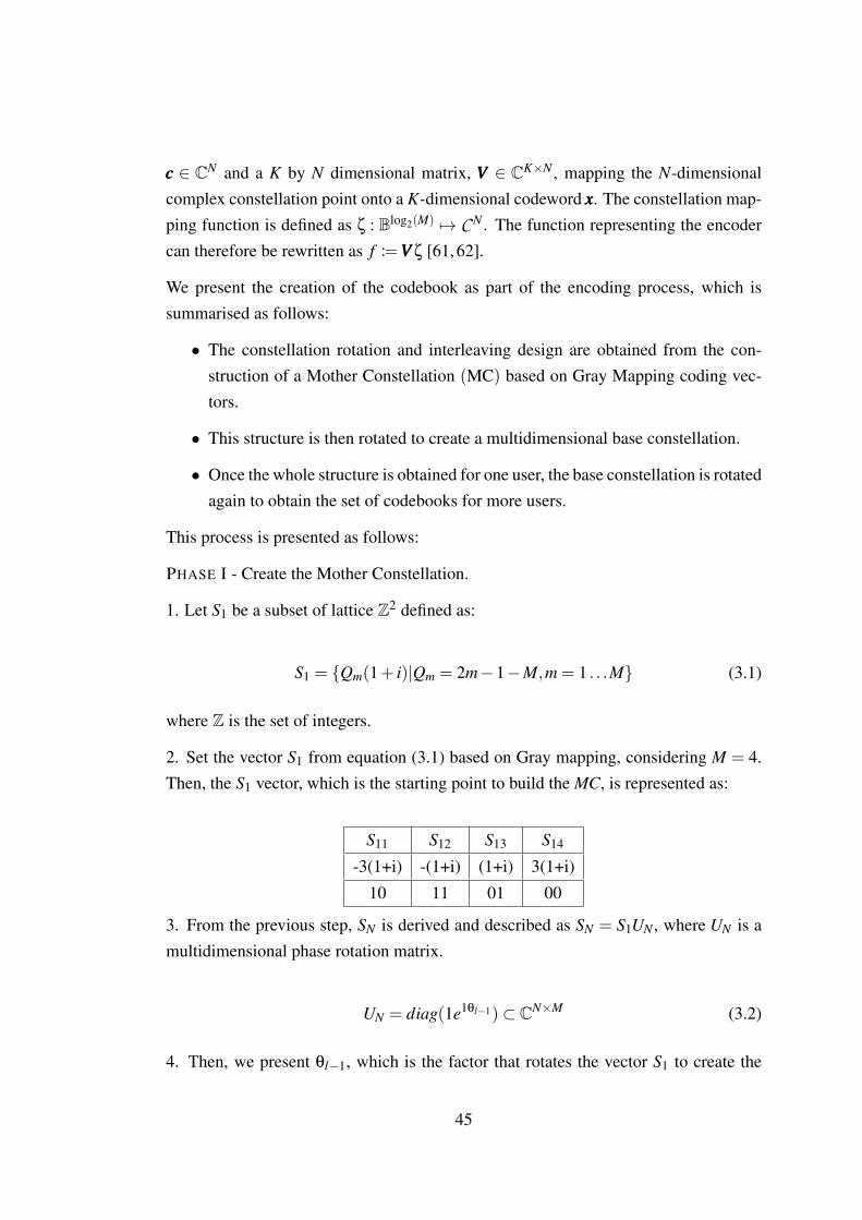
1. Let S1 be a subset of lattice Z2 defined as:

S1 = {Qm(1+ i)|Qm = 2m−1−M,m = 1 . . .M} (3.1)

where Z is the set of integers.

2. Set the vector S1 from equation (3.1) based on Gray mapping, considering M = 4.Then, the S1 vector, which is the starting point to build the MC, is represented as:

S11 S12 S13 S14

-3(1+i) -(1+i) (1+i) 3(1+i)

10 11 01 00

3. From the previous step, SN is derived and described as SN = S1UN , where UN is amultidimensional phase rotation matrix.

UN = diag(1e1θl−1)⊂ CN×M (3.2)

4. Then, we present θl−1, which is the factor that rotates the vector S1 to create the

45

multi-dimension in the MC. In Figure 3.2, the MC is illustrated, using the base vectorS1 and the N dimensions after rotating the vector, and it is defined as:

θl−1 = (l−1)× π

MN, l = 1, . . . ,N (3.3)

Figure 3.2: Rotation of vector S1 to obtain the Mother Constellation [60]

5. After rotating the SN vector, the N-dimensional matrix MC with M points can beexpressed as:

MC = (S1, . . .SN)T =

S11 S12 . . . S1M

...... . . .

......

... . . ....

SN1 SN2 . . . SNM

6. The interleaving and reordering of the elements in the vector is needed to improvethe performance of the codewords in the presence of fading. It is done as follows:

6a) Select the even dimensions (rows) in the MC and reorder them. For example, theSe vector after interleaving is S′e, where e is an even element of N and it can be writtenas:

46

S′e = {−Se,M/2+1, . . . ,−Se,3M/4,Se,3M/4+1, . . . ,−Se,M,Se,M, . . . ,

−Se,3M/4,Se,3M/4, . . . ,Se,M/2+1} (3.4)

6b) After this step, the MC is represented as:

MC = (S1, . . . ,S′e, . . . ,SN)T (3.5)

7. For simplification and to calculate the MC, let us set N = 2 and M = 4. From Step1 and 2 we have the elements of the S1 vector as follows:

S11 =−3(1+ i), S12 =−(1+ i), S13 = (1+ i), S14 = 3(1+ i)

8. We calculate the angle of rotation phases in the MC from equation (3.3) as fol-lows:

For l = 1 and for l = 2, we have:

θ1−1 = θ0 =(1−1)π(4)(2) = 0 and θ1−2 = θ1 =

(2−1)π(4)(2) = π

8 .

The angles θ0 = 0 and θ1 = π/8 ensure that the minimum square Euclidean distancehas been maximized for the MC, as proved in the design presented in [60].

9. The angles rotate the initial vector and determine the dimensions of the MC. Weobtain SN =UNS1 from equation (3.2), then we have UN = diag(1eiθl−1).

9a) For θ0 = 0, we have

S1 =

1+0i 0 0 0

0 1+0i 0 00 0 1+0i 00 0 0 1+0i

−3−3i

−1−1i

1+1i

3+3i

=

−3−3i

−1−1i

1+1i

3+3i

as a result:

S11 =−3−3i

S12 =−1−1i

S13 = 1+1i

S14 = 3+3i

47

9b) For θ1 =π

8 , we have

S2 =

ei π

8 0 0 00 ei π

8 0 00 0 ei π

8 00 0 0 ei π

8

−3−3i

−1−1i

1+1i

3+3i

=

−1.62−3.92i

−0.54−1.31i

0.54+1.31i

1.62+3.92i

as a result

S21 =−1.62−3.92i

S22 =−0.54−1.31i

S23 =0.54+1.31i

S24 =1.62+3.92i

10. After we have obtained the S vectors, we finish the interleaving process for theeven numbered S vectors. S2, represented by Se, will be modified as shown in equation(3.4) before the interleaving.

Se1 =S21 = −3(1+ i)ei π

8 ,

Se2 =S22 = −(1+ i)ei π

8 ,

Se3 =S23 = (1+ i)ei π

8 ,

Se4 =S24 = 3(1+ i)ei π

8

As in this example, e= 2, we have S′e = S′2 therefore after the interleaving, we have:

S′21 =S′e1 = S22 =− (1+ i)ei π

8 ,

S′22 =S′e2 = S24 =3(1+ i)ei π

8 ,

S′23 =S′e3 = S21 =−3(1+ i)ei π

8 ,

S′24 =S′e4 = S23 =(1+ i)ei π

8

11. Then, MC = (S1,S′2)T , where the final MC is represented as:

MCMCMC =

[ 00 01 10 11

S1 −3.00−3.00i −1.00−1.00i 1.00+1.00i 3.00+3.00i

S2 −0.54−1.31i 1.62+3.92i −1.62−3.92i 0.54−1.31i

]

48

PHASE II - Populate the complex Mother Constellation onto the sparse codewords.A codebook X j for a single user is generated by concatenating the codewords corre-sponding to different symbols transmitted by the user j. We represent each symbol inthe codebook with a column vector containing K rows. Two of the rows are populatedwith complex numbers and two contain the value 0. Therefore, the SCMA codebook,known as X j for j-th user, is created as follows [61]:

X j =Vj∆ jMC, j = 1,2, . . . ,J (3.6)

1. The dispersion matrix for each user sparsely populated is Vj, whereVVV ∈BK×N , map-ping the N-dimensional complex constellation point onto a K-dimensional codewordxxx.

For this case, when K = 4, N = 2 and J = 6, the matrices Vj, j = 1 . . .J are:

V1 =

1 00 00 10 0

V2 =

0 01 00 10 0

V3 =

0 00 01 00 1

V4 =

1 00 10 00 0

V5 =

1 00 00 00 1

V6 =

0 01 00 00 1

2. The codebook construction for different users requires that the Mother Constellationis rotated. The angles phase rotation are expressed:

φu = (u−1)2π

Mdf+ eu

2π

M,∀u = 1, . . . ,df (3.7)

49

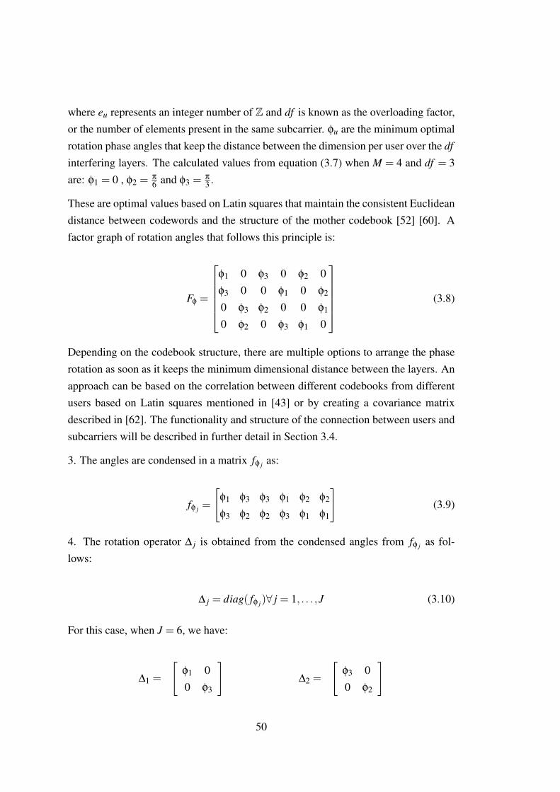
where eu represents an integer number of Z and df is known as the overloading factor,or the number of elements present in the same subcarrier. φu are the minimum optimalrotation phase angles that keep the distance between the dimension per user over the df

interfering layers. The calculated values from equation (3.7) when M = 4 and df = 3are: φ1 = 0 , φ2 =

π

6 and φ3 =π

3 .

These are optimal values based on Latin squares that maintain the consistent Euclideandistance between codewords and the structure of the mother codebook [52] [60]. Afactor graph of rotation angles that follows this principle is:

Fφ =

φ1 0 φ3 0 φ2 0φ3 0 0 φ1 0 φ2

0 φ3 φ2 0 0 φ1

0 φ2 0 φ3 φ1 0

(3.8)

Depending on the codebook structure, there are multiple options to arrange the phaserotation as soon as it keeps the minimum dimensional distance between the layers. Anapproach can be based on the correlation between different codebooks from differentusers based on Latin squares mentioned in [43] or by creating a covariance matrixdescribed in [62]. The functionality and structure of the connection between users andsubcarriers will be described in further detail in Section 3.4.

3. The angles are condensed in a matrix fφ j as:

fφ j =

[φ1 φ3 φ3 φ1 φ2 φ2

φ3 φ2 φ2 φ3 φ1 φ1

](3.9)

4. The rotation operator ∆ j is obtained from the condensed angles from fφ j as fol-lows:

∆ j = diag( fφ j)∀ j = 1, . . . ,J (3.10)

For this case, when J = 6, we have:

∆1 =

[φ1 00 φ3

]∆2 =

[φ3 00 φ2

]

50

∆3 =

[φ3 00 φ2

]∆4 =

[φ1 00 φ3

]

∆5 =

[φ2 00 φ1

]∆6 =

[φ2 00 φ1

]Therefore, the SCMA codebook, known as X j for j-th user is expressed as:

X j =Vj∆ jMC, j = 1,2, . . . ,J (3.11)

For example, for j = 1:

X1 =

1 00 10 00 0

[

φ1 00 φ3

][S11 S12 S13 S14

S′21 S′22 S′23 S′24

]

=

1 00 00 10 0

[

e0 00 e

π

6

][−3.00−3.00i −1.00−1.00i 1.00+1.00i 3.00+3.00i

−0.54−1.31 j 1.62+3.92i −1.62−3.92i 0.54−1.31i

]

then, after normalising the values we have X1

X1 =

00 01 10 11

SC1 −0.5741−0.5741i −0.2807−0.2807i 0.2807+0.2807i 0.6461+0.6461i

SC2 0.0000+0.0000i 0.0000+0.0000i 0.0000+0.0000i 0.0000+0.0000i

SC3 0.0358−0.2688i −0.1563+1.1801i 0.1563−1.1801i 0.2418−0.1862i

SC4 0.0000+0.0000i 0.0000+0.0000i 0.0000+0.0000i 0.0000+0.0000

For j = 2 . . .J, the codebooks are:

51

X2 =

00 01 10 11

SC1 0.0000+0.0000i 0.0000+0.0000i 0.0000+0.0000i 0.0000+0.0000i

SC2 −0.2101−0.7842i −0.1027−0.3834i 0.1027+0.3834i 0.2365+0.8827i

SC3 0.1654−0.2148i −0.7255+0.9438i 0.7255−0.9438i 0.3025−0.0404i

SC4 0.0000+0.0000i 0.0000+0.0000i 0.0000+0.0000i 0.0000+0.0000i

X3 =

00 01 10 11

SC1 0.0000+0.0000i 0.0000+0.0000i 0.0000+0.0000i 0.0000+0.0000i

SC2 0.0000+0.0000i 0.0000+0.0000i 0.0000+0.0000i 0.0000+0.0000i

SC3 −0.2101−0.7842i −0.1027−0.3834i 0.1027+0.3834i 0.2365+0.8827i

SC4 0.1654−0.2148i −0.7255+0.9438i 0.7255−0.9438i 0.3025−0.0404i

X4 =

00 01 10 11

SC1 −0.5741−0.5741i −0.2807−0.2807i 0.2807+0.2807i 0.6461+0.6461i

SC2 0.0358−0.2688i −0.1563+1.1801i 0.1563−1.1801i 0.2418−0.1862i

SC3 0.0000+0.0000i 0.0000+0.0000i 0.0000+0.0000i 0.0000+0.0000i

SC4 0.0000+0.0000i 0.0000+0.0000i 0.0000+0.0000i 0.0000+0.0000i

X5 =

00 01 10 11

SC1 0.2020−0.7538i 0.1131−0.4222i −0.1131+0.4222i −0.3862+1.4413i

SC2 0.0000+0.0000i 0.0000+0.0000i 0.0000+0.0000i 0.0000+0.0000i

SC3 0.0000+0.0000i 0.0000+0.0000i 0.0000+0.0000i 0.0000+0.0000i

SC4 −0.0993−0.2410i 0.5007+1.2116i −0.5007−1.2116i 0.1899−0.4607i

X6 =

00 01 10 11

SC1 0.0000+0.0000i 0.0000+0.0000i 0.0000+0.0000i 0.0000+0.0000i

SC2 0.2020−0.7538i 0.1131−0.4222i −0.1131+0.4222i −0.3862+1.4413i

SC3 0.0000+0.0000i 0.0000+0.0000i 0.0000+0.0000i 0.0000+0.0000i

SC4 −0.0993−0.2410i 0.5007+1.2116i −0.5007−1.2116i 0.1899−0.4607i

52

3.2 SCMA transmission

We consider an SCMA uplink multiuser system, serving a group of j ∈ (1,... , J)

users that are sharing k ∈ (1,... , K) subcarriers. Figure 3.3 shows the principle ofSCMA users transmitting to the base station (BS). The BS will provide the users withinformation regarding codebook assignment as well as resource allocation, after thecodebooks are generated, this process is visited in further detail in Section 3.1. Thisprocess is based on constellation rotation and the interleaving method. In particular,the first dimension is constructed using a Mother Constellation with Gray mappingvectors and interleaving. The other dimensions are then obtained by rotating the firstdimension via a rotation operator and multiplying the resulting constellation by eachunique user’s sparse matrix [60]. Finally, a codeword (codebook pattern) will be se-lected from the user’s codebook to represent a sequence of bits for each user.

Figure 3.3: SCMA system transmission representation

The codewords are multiplexed with the other users’ codewords over the k sharedorthogonal resources, resulting in a k-th vector. The compound vector y is the math-ematical representation of the user’s signal received at the base station, representedgraphically in Figure 3.4.

53

Figure 3.4: Graphic representation of the codebooks and multiplexed signals

The users will be located at different distances from the base station, and with theeffect of path loss and fading, each of them will experience different channel gain. Itis assumed that the BS and the users have perfect knowledge of the CSI. The channelgain for the j-th user at subcarrier k is expressed as |hk, j|2 =

ε|Hk, j|2PL . The users are

uniformly distributed around the BS with the presence of path loss (PL), log-normalshadowing ε and a frequency selective fading gain of |Hk, j|2 [25, 27]. The gain can berepresented by the matrix h such that:

h =

h1,1 h1,2 . . . hk,6

...... . . .

......

... . . ....

h4, j h4,2 . . . hK,J

for j = 1...J and k = 1...K (3.12)

Each of the k elements of the noise vector nk satisfy the characteristic nk ∼ CN(0,σ2),which means they follow a complex valued normal random variable with mean µo = 0and variance σ2. We can express the transmitted signal on the uplink channel, asreceived at the base station, as follows:

54

yk =J

∑j=1

hk, jxk, j +nk,∀k = 1 . . .K (3.13)

The parameter that will determine the sparsity in the codewords, expressed as xk, j, isthe number of subcarriers which are allocated to each user’s codewords, better knownas the spreading factor dv over the total number of subcarriers. The number that repre-sents the amount of users assigned to a subcarrier is known as the overloading factor df .The overloading with respect to the number of symbols is determined by the ratio of thenumber of users sharing the same subcarrier (df = 3) to the number of subcarriers peruser (dv = 2), resulting in df

dv = 1.5. The non-zero N elements on each codeword needto be fewer in number than the number of subcarriers in order to call the system sparse.These values will define the complexity and the characteristics of the codebook’s de-sign. The size of the codebook will be maximised when N = K/2 [63]. As an example,we present a numerical exercise to obtain the resultant signal y in Appendix A.

3.3 SCMA receiver and signal detection

After the superposed signal has been transmitted to the base station, the signal mustbe detected and decoded into symbols. This action is performed by the base stationwith previous knowledge of the codebooks for each user and channel mappings. Thereceived signal is detected based on MPA, as shown in Figure 3.1 (Section 3). Oncethe interference from other users is removed, the resultant signal is processed andcompared against the codewords in the codebooks to find the set of codewords withthe highest likelihood of being transmitted. After the comparison with the knowncodewords, the receiver selects the binary values corresponding to these codewords asthe decoded signal. The accuracy of the detection process in SCMA is affected by avariety of factors, including codebook design, channel performance and interference[48–50].

One effective way of performing the detection of the symbols sent by each user is Mes-sage Passing Algorithm (MPA) also known as belief propagation (BP) algorithm [64].MPA operates by passing the message through the nodes along the edges in a factorgraph until a maximum number of iterations is reached and uses the sum-product ineach iteration to calculate joint probabilities of different codewords based on Bayesianprinciples. In order to obtain the probability calculation of the transmitted symbols, the

55

numerical values of the received vector and the probability of the codewords within theuser’s codebooks are required [64].

For practical purposes and to illustrate the detection process, we consider one of thetechniques that implements MPA at the receiver based on [55, 65]. In this case, eachuser presents their own codebook containing four codewords to choose from, assumingthat all users will transmit a codeword within a data frame. As we have no knowledgeof the data that is to be transmitted and assume that each codeword is selected by a userwith equal likelihood (note that due to their nature, efficient compression, encryptionand source coding/compression will produce data streams which use all symbols withroughly equal probability) we can set the initial probability of a user choosing a givencodeword to be 1 divided by the cardinality of the set of codewords in a user’s code-book, as shown in equation (3.14). Thus, all codewords will have an initial probabilityof 1

4 as each user has four of them,

Pr(0)VkFn(xk

n) =1∣∣Xkn∣∣ , Pr(0)ViFn

(xin) =

1∣∣X in∣∣ , Pr(0)V jFn

(x jn) =

1∣∣X jn∣∣ (3.14)

where Pr(0)VkFnis the initial probability of a node connected to a function. xk

n, xin and

x jn are the estimated transmitted symbols for each user (k, i, j) present in the node n

and Xkn , X i

n and X jn are the corresponding codebooks of user k, i and j.

∣∣ · ∣∣ denotescodebook cardinality.

Subsequently, a connected graph is formed, containing nodes corresponding to theusers and subcarriers in order to propagate the probability calculation, as depicted inFigure 3.5. For this example, we have six variable nodes representing users and fourfunctional nodes (sometimes also known as factor or check nodes in some literature)representing subcarriers. Edges between functional and variable nodes represent thata user is carried by a given subcarrier or that a subcarrier is carrying a given user.Probabilities calculated at each step of the process can be said to be sent betweenconnected nodes along these edges. From the connected graph in Figure 3.5 , we cansee that each user uses two subcarriers to transmit its signal (so each variable node haslines exiting it to connect to two functional nodes) and each subcarrier is shared bythree users, therefore, it has three lines entering it.

56

V1 V2 V3 V4 V5 V6

F1 F2 F3 F4

Variablenodes(layers)

Functionnodes

(resources)

Figure 3.5: Graph showing the connection of variable nodes with function nodes.

The initial probabilities of each codeword will be the entry value to a function whichrepresents a functional node. The function uses these values and the difference fromthe received signal vector to calculate the probability of the codeword in the receivedvector corresponding to the subcarrier.

The functional node then supplies each variable node with the probability that each ofits codewords corresponded to the received signal vector when combined with code-words from the other two nodes connected to that functional node. These probabilitiesare then normalised in order to make them sum to one at the variable node and passedto the functional node, in place of the initial probabilities, for the next iteration of theprocess. A higher number of iterations can achieve a greater level of accuracy in thedecoded signal. Figure 3.6 illustrates the iterative process of MPA [66].

57

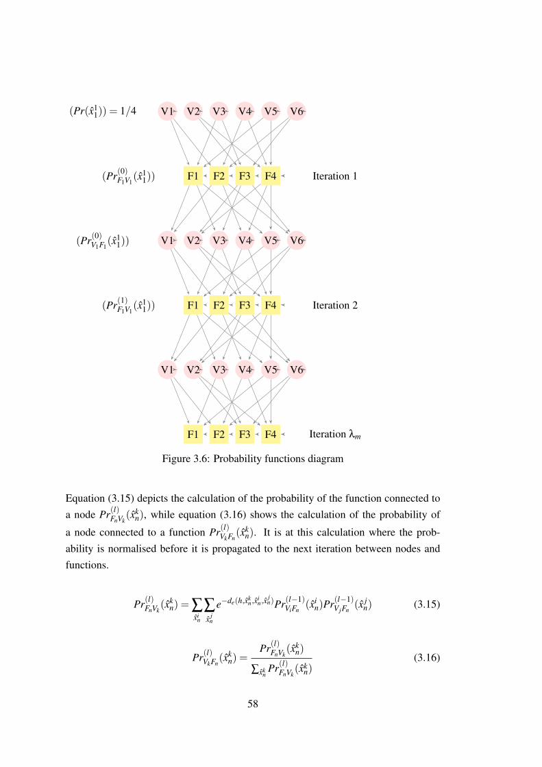
V1 V2 V3 V4 V5 V6

F1 F2 F3 F4

(Pr(x11)) = 1/4

Iteration 1(Pr(0)F1V1(x1

1))

V1 V2 V3 V4 V5 V6

F1 F2 F3 F4 Iteration 2

V1 V2 V3 V4 V5 V6

F1 F2 F3 F4 Iteration λm

(Pr(0)V1F1(x1

1))

(Pr(1)F1V1(x1

1))

Figure 3.6: Probability functions diagram

Equation (3.15) depicts the calculation of the probability of the function connected toa node Pr(l)FnVk

(xkn), while equation (3.16) shows the calculation of the probability of

a node connected to a function Pr(l)VkFn(xk

n). It is at this calculation where the prob-ability is normalised before it is propagated to the next iteration between nodes andfunctions.

Pr(l)FnVk(xk

n) = ∑xi

n

∑x j

n

e−de(h,xkn,x

in,x

jn)Pr(l−1)

ViFn(xi

n)Pr(l−1)V jFn

(x jn) (3.15)

Pr(l)VkFn(xk

n) =Pr(l)FnVk

(xkn)

∑xknPr(l)FnVk

(xkn)

(3.16)

58

From both equations, l is the number of the iteration to decode the symbols of the usersthat are sharing the same resource.

de(h, xkn, x

in,x

jn) = |yn− (hk

nxkn +hi

nxin +h j

nx jn)|2 (3.17)

Equation (3.17) obtains the Euclidean distance between the transmitted signal and thesymbols for each user (k, i and j) per function node, expressed as:

xkn, x

in, x

jn (3.18)

The marginal probability of each codeword is calculated for each user, after the pre-vious step, by multiplying the two functional node outputs relating to that user. Thisproduces a resultant marginal probability value for each of a user’s codewords. Next,the codeword with the highest marginal probability is selected for each user, andthe bitstreams corresponding to the selected codewords are the data output for thatuser [65].

Having the received compound signal y = [y1,y2, ...,yn], the knowledge of the channelh and the value of the joint maximum a-posteriori probability (MAP) the detection willbe expressed as:

x = argx∈X1∗...∗X jmax Pr(X/y) (3.19)

where x is the expected codeword from the codebook and X is the known value of thecodebook.

3.4 Factor graph design and sparsity

We have explained how users will be spread over subcarriers and how the subcarrierswill be connected to users in a connected graph, as presented in Figure 3.5. This will berepresented by a matrix F = [ fk, j] with entries (0,1) that shows the mapping betweenusers and subcarriers. If fk j = 1, it indicates that a user is allocated to a particularsubcarrier and otherwise if it is 0. The number of users contributing to each subcarrierwill be defined by d f k = (d f 1, ...,d f K)

T = ∑Jj=1 f j

59

FFF =

1 0 1 0 1 01 0 0 1 0 10 1 1 0 0 10 1 0 1 1 0

(3.20)

3.5 Sparsity of codewords

The parameter that will determine the sparsity of the codewords is the number of avail-able subcarriers K minus the number of effective subcarriers (allocated subcarriers)represented by dv, also known as the spreading factor over the subcarriers. The non-zero N elements on each codeword need to be fewer in number than the number oftotal subcarriers in order to call the system sparse. These values will determine thecomplexity and characteristics of the codebook, given by the calculation

(NK

). The size

of the codebook is maximised when N = K/2.

Having this combinatorial number, we can now calculate the size of the codebooks,which will be greatly increased when the number of subcarriers increases, while main-taining sparsity and its advantages. For instance, for K = 4 and N = 2, the number ofcodebooks generated will be 6, corresponding to the number of users. However, forK = 12 and N = 6, the number of codebooks generated will be 924 [63].

3.6 Numerical results

In this section, we present link-level simulation results from the SCMA and PDMAsystems, in order to illustrate the functionality and importance of each element in-volved in the transmission and detection processes of the coded NOMA systems. Wehave simulated SCMA and PDMA systems in MATLAB (PDMA is described in fur-ther detail in Section 5). The simulations include uplink scenarios with a single cell andJ users, which are uniformly distributed from the base station with total transmissionpower Pt and bandwidth divided into K number of subcarriers. The codebook for thetransmitted signal has been generated based on the process presented in Section 3.1.For the receiver in the system the initial probability of each symbol is 1/4. The wire-less channel is modelled as a Rayleigh fading channel with Additive White GaussianNoise (AWGN) as described in Section 3.2. The simulation results have been carriedout using the Monte Carlo method with the parameters in Table 3.1 as follows:

60

Parameters SCMA Values PDMA Values

Number of users 6 6

Number of codebooks 6 6

Subcarriers 4 4

Sparsity 2 -

Overloading of symbols 1.5 1.5

Factor overloading 3 2

Factor spread 2 -

Factor spread for overlay users - 2

Factor spread for underlay users - 1

Pedestrian model B B

PL exponent 3 3

Bandwidth 180 kHz 180 kHz

Noise -174 dBm -174 dBm

Shadowing 8dB 8dB

Transmit power 0-23dBm 0-23dBm

Initial probability 1/4 1/4

Monte Carlo iterations 10 000 10 000

Table 3.1: Parameters of link performance simulation for SCMA and PDMA

As part of the simulation of the SCMA system, we include BER simulations of theoverall system in Figure 3.7 and BER per user in Figure 3.8. This provides an illus-trative example of the performance of the codebook design and the detection processrelative to the transmission bit error rate.

61

Figure 3.7: BER performance of SCMA system in the uplink for the purpose of com-parison with PDMA

It must be noted that although this work does not investigate the codebook design oreffectiveness of the detection process, it is important to simulate the average BER ofthe system in order to provide a framework for comparison with further code domainmultiple access techniques such as PDMA.

62

Figure 3.8: BER performance of SCMA systems in the uplink per user

The average BER results presented in Figure 3.9 aim to compare the performance ofSCMA and PDMA systems. We simulate a system with a similar codebook struc-ture to the one presented in the SCMA system. It has been proved that the sparsity inthe codebook is directly connected to the factor graph in coded based systems. How-ever, the PDMA factor graph has lower density than the one presented for SCMA. Wecan see from the blue line in Figure 3.9 that the performance can be considerably de-graded with a less dense codebook. The decoding process of the transmitted symbolsin PDMA is applied in the same manner as the decoding process applied for the usersin SCMA presented in Section 3.3. This is possible due to the similarity of structurewith the pattern presented in PDMA. The differences are in the sparse codes for theusers ( j = 3 . . .J). This does not impact the implementation of the decoder, however,higher diversity will impact the complexity of the detection process.

63

Figure 3.9: Comparison of average BER in SCMA vs PDMA systems

Figure 3.10 presents the BER results per user in order to compare those users withdifferent pattern allocation and the direct impact on the performance. The users withlower density patterns present higher BER than those with higher density patterns.

64

Figure 3.10: BER per user in PDMA system. The users are ordered from low BER tohigh BER. User 1 shows the lowest BER and user 6 shows the highest BER.

3.7 Chapter summary

As in the case of SCMA, coded NOMA in the uplink has been of interest to researchersas the technique is able to accommodate several users by overloading the subcarriers.In this chapter, the system of SCMA has been described in detail in order to under-stand and implement the elements that are part of the system. We have focused specialattention on the implementation of the codebook design and a particular decoding tech-nique. Due to the complexity of the codebooks and detection techniques and for prac-tical purposes, implementation examples are supplied for specific cases. Numericalresults are provided to support the description of the systems and show the link perfor-mance evaluation. Results are also provided for the PDMA system described later inChapter 5 of this work. BER comparisons per system and per user are presented. Thischapter established the main principles of SCMA, which provides grounds for the nextissue to investigate in order to enhance the system, namely resource allocation.

65

Chapter 4

Resource allocation for Uplink SCMASystem

Resource allocation plays a vital role in multiple access techniques. Non-orthogonalaccess has many advantages over its predecessors and as shown in previous work,accurate resource allocation algorithms are essential to ensure the inherent capabilitiesof multiple access. Through this chapter, we will demonstrate how in order to exploitthe full potential of code domain NOMA an efficient and practical subcarrier and powerallocation solution is needed.

We have mentioned before that the assignment of resources can be approached in twostages. Previous work on SCMA has been implemented in a similar manner. Workin [67] has placed special emphasis on subcarrier allocation using matching theory.On the other hand, in that research power allocation was overlooked by using a simplewaterfilling method and not taking interference from other users into account. Workin [62] has solved the subcarrier allocation problem by using an algorithm where ineach iteration one user is allocated at a time per resource until all the possible code-book patterns are exhausted. However in the same work, power allocation is solvedwith a numerical calculation using the convex tools in MATLAB. The problem ofinterference is widely common in multiple user systems and has been of interest tooptimisation experts. In the work presented in [32], in the NOMA uplink system aresource allocation solution has been explored, using matching theory and the waterfilling principle but taking the interference into account. This work has been very use-ful even when the subcarrier allocation constraints are not included and no minimum

66

rate is considered. The authors of [29] presented a system combining PD-NOMAand CD-NOMA techniques to support an increased number of users. Using powerdomain NOMA, additional low data rate users were superimposed onto an SCMA sys-tem. D2D transmission and matching theory in the uplink have been explored in [68],which provided deeper knowledge of MT and its complexity.

4.1 SCMA capacity and resource allocation

In the previous chapter, we have described the components of the SCMA system andits characteristics. We have witnessed the importance of maintaining the pattern of thecodebook.

From the Shannon’s capacity equation and based on power NOMA uplink, we canderive the SCMA rate total equation. The binary variable fk, j indicates whether auser j is allocated to a particular subcarrier k, and the mobile equipment has a limitedtotal power Pmax

j , which is split between dv subcarriers of equal bandwidth B. Thetransmission power of user j allocated to subcarrier k is expressed as pk, j. The rate persubcarrier k can be depicted as [32]:

Rk = BJ

∑j=1

log2(1+fk, j pk, j|hk, j|2

BNo + Ik, j) (4.1)

where Ik j is the interference caused by the other users over the subcarrier k, expressedas:

Ik, j =J

∑i=1,i 6= j

fk,i pk,i|hk,i|2 (4.2)

In previous sections, the SCMA system has been described and we have presentedthe challenge of this technique. The objective of the system is to transmit the highestamount of information by the best management of the available resources such as theones optimised in this work; power and subcarriers. In order to solve this problem, itneeds to be split into two sub-problems, which need to be solved independently, thus,a suboptimal joint solution is presented.

67

4.2 Subcarrier allocation for SCMA

SCMA benefits from allocating multiple users to the same resources by increasing theoverall transmission rate, however, the codebook constraints can limit the effect of thisfeature due to the number of users that can be assigned to a specific subcarrier andthe restriction of duplicated codebook patterns. These constraints and the presence ofmultiple users will generate high interference between them. Although this negativeeffect is partly mitigated by the sparsity of the codebook, subcarrier allocation will berequired to improve the performance of the transmission rate.

In this research, different subcarrier allocation methods were carried out in order tocompare method complexity and the effect of each method on the total rate perfor-mance [43], [67], [69], [70]. In this section, a proposed low complexity algorithm isdescribed and presented to solve the problem of subcarrier allocation.

4.2.1 Greedy algorithm based methods

There are several approaches to solve heuristic problems. The greedy algorithm isknown for being able to find solutions by solving the problem in local stages, not con-sidering the global problem or whole picture. Additionally, algorithms based on thisprinciple are usually capable of achieving good results with moderate complexity re-quirements. Whilst the optimal global solution may not be identified, greedy algorithmapproaches often obtain a near-optimal or acceptable solution under specific purposes,using minimal computational complexity [71,72]. For this reason, it is worth exploringdifferent subcarrier allocation schemes using this principle as minimising resource useis an important factor in mobile equipment applications. For this particular problem,exhaustive search will be used to find the global optimal solution in order to produce anupper bound indicator for the proposed algorithms. Random or fixed subcarrier alloca-tion will be presented to establish a lower bound indicator for this comparison.

4.2.1.1 Proposed subcarrier allocation algorithm

User-subcarrier mapping fk, j,∈ [0,1], from equation (4.1), is the discrete variable inthe capacity equation of SCMA that requires optimisation. In order to solve this sub-problem, we have designed a subcarrier algorithm that is presented as follows:

1: Let A be a set of possible codebook pattern assignments ai ∈ A {0,1}.

68

2: All the possible K-rowed binary column vectors from the codebook [57, 60], whichcontain dv number of ones and (K− dv) number of zeros, are defined as codebookpattern assignments.

3: F is defined as a matrix with dimensions (J×K) representing user-subcarrier allo-cations. We initialise it as a zero-value matrix F = 0K,J and complete each column byusing the following algorithm.

First, a random pattern is selected from all the possible patterns for user 1, and theoverall rate is calculated, assuming no interference as all the other users are not yetallocated. The vector that achieves the highest rate is allocated and is deleted from A,A′ = A\a as shown in Figure 4.1.

Figure 4.1: Graphic representation of first user’s subcarrier allocation

We proceed to the adjacent user and the opposite pattern a is selected, for instance,as shown in Figure 4.2. This is deleted from the set of available codebook patternassignments A′′ = A′ \ a.

For the odd numbered user j = (2n+1), the overall rate is calculated in order to selectthe best pattern allocation. We allocate even numbered users j = (2n) the opposite pat-tern compared to the previous odd user, as represented in Figure 4.2. Used assignmentsare deleted from the set of available codebook pattern assignments at each stage.

69

Figure 4.2: Graphic example of odd and even numbered users’ subcarrier allocation

This process should continue until all the users are allocated a codebook pattern asdescribed in Algorithm 1.

Algorithm 1 Proposed subcarrier algorithm1: Inputs:

K,J,dv,h2: Initialize:

n = 0 and F = 0K,J3: A = { all possible user-subcarrier assignment vectors}4: Select dv subcarriers with highest channel gain from h5: Set the corresponding row values in column 1 of F to 16: Set column 2 of F to the binary inverse of column 1.7: Delete the vectors matching columns 1 and 2 F from A8: do9: Let n = n+1 and j = 2n+1

10: Calculate the rate obtained when each vector from A is used in position j of F11: Select vector ai ∈ A which gives the best performance.12: Assign the selected member of A to column j of F13: Set the values of column j+1 to the inverse of those in column j14: Delete vectors matching Fj and Fj+1 from A, where Fj is the j-th column vector

of F15: while n < (J/2)16: Obtain F*

70

4.2.1.2 Low complexity proposed algorithm

Computational complexity is an element that should be considered in subcarrier al-location methods. For this reason, a low complexity algorithm based on the greedyprinciple is proposed in this work (Algorithm 1, Section 4.2.1.1) with the aim of satis-fying the limitation of the power and processing of the mobile equipment with respectto the base station. The proposed algorithm is able to achieve a close to optimal so-lution while reducing the operations and the number of iterations. Thereby savingconsiderable computational resources such as time and computing processing, whichcan facilitate the practical implementation. The exhaustive search is affected by thenumber of permutations, the number of users to be allocated and the calculation of thetotal rate in every iteration, which results in O(J!). The complexity of the proposedsubcarrier allocation algorithm in SCMA can be obtained based on the following cal-culations:

• The complexity is determined by the rate calculation operations and the numberof elements in the greedy algorithm (J). Using the opposite pattern allocationfor even numbered users reduces the number of operations required in the greedyprocess to (J−df ).

• The number of rate calculation operations is given by (df ).

• Therefore, we can express the complexity as O((J−df )2).

4.2.2 Matching Theory

Matching theory is a tool used to generate a dynamic relation among a set of playerscompeting for their own individual benefits. It has been widely used in different dis-ciplines from economics to sociology since its first appearance with the work of Galeand Shapley on the stable marriage and college admission problems in 1962 [73]. Ithas recently been applied in wireless communications theory to deal with the interac-tion between rational and selfish resources [74] [75] [76]. For instance, in [77], MTis applied in OFDMA systems to assign the users to the available resources. In [78],the authors aim to optimize the sub-channel assignment to achieve a balance betweenthe number of scheduled users and total sum rate maximization. The work presentedin [79] proposes a Matching Theory resource allocation solution for MIMO cognitiveradio links. There are variants of matching theory such as: one to one, many-to-oneand many-to-many. The most well known and used is the one to one approach, which is

71

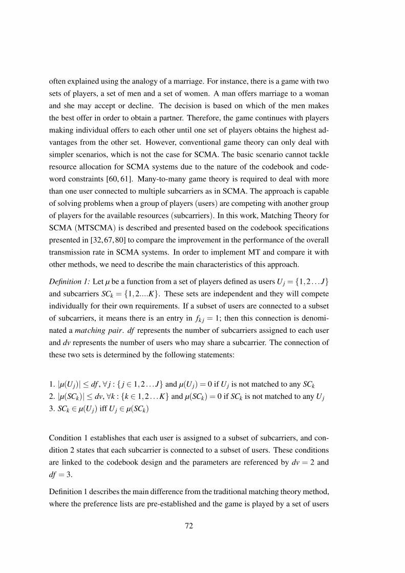
often explained using the analogy of a marriage. For instance, there is a game with twosets of players, a set of men and a set of women. A man offers marriage to a womanand she may accept or decline. The decision is based on which of the men makesthe best offer in order to obtain a partner. Therefore, the game continues with playersmaking individual offers to each other until one set of players obtains the highest ad-vantages from the other set. However, conventional game theory can only deal withsimpler scenarios, which is not the case for SCMA. The basic scenario cannot tackleresource allocation for SCMA systems due to the nature of the codebook and code-word constraints [60, 61]. Many-to-many game theory is required to deal with morethan one user connected to multiple subcarriers as in SCMA. The approach is capableof solving problems when a group of players (users) are competing with another groupof players for the available resources (subcarriers). In this work, Matching Theory forSCMA (MTSCMA) is described and presented based on the codebook specificationspresented in [32,67,80] to compare the improvement in the performance of the overalltransmission rate in SCMA systems. In order to implement MT and compare it withother methods, we need to describe the main characteristics of this approach.

Definition 1: Let µ be a function from a set of players defined as users U j = {1,2 . . .J}and subcarriers SCk = {1,2....K}. These sets are independent and they will competeindividually for their own requirements. If a subset of users are connected to a subsetof subcarriers, it means there is an entry in fk j = 1; then this connection is denomi-nated a matching pair. df represents the number of subcarriers assigned to each userand dv represents the number of users who may share a subcarrier. The connection ofthese two sets is determined by the following statements:

1. |µ(U j)| ≤ df , ∀ j : { j ∈ 1,2 . . .J} and µ(U j) = 0 if U j is not matched to any SCk

2. |µ(SCk)| ≤ dv, ∀k : {k ∈ 1,2 . . .K} and µ(SCk) = 0 if SCk is not matched to any U j

3. SCk ∈ µ(U j) iff U j ∈ µ(SCk)

Condition 1 establishes that each user is assigned to a subset of subcarriers, and con-dition 2 states that each subcarrier is connected to a subset of users. These conditionsare linked to the codebook design and the parameters are referenced by dv = 2 anddf = 3.

Definition 1 describes the main difference from the traditional matching theory method,where the preference lists are pre-established and the game is played by a set of users

72

with just one offer at a time. In the many-to-many approach adapted to resource alloca-tion for SCMA uplink, the swap operation, known as any possible exchange betweenany set of players and its offers, continues until the rate conditions are accomplished.The swap matching is defined as:

Az(µ)i ji′ j′ = {µ /∈ {(i,µ(i)),(i′,µ(i′))}}∪{(i,{{µ(i) /∈ { j}}∪{ j′}}),

(i′,{{µ(i′) /∈ { j′}}∪{ j}})} (4.3)

where j ∈ µ(i) and j′ ∈ µ(i′) and j′ /∈ µ(i) and j /∈ µ(i′). This statement means thata pair of users can exchange one of their matched resources with each other whilekeeping the other subcarrier unchanged.

Definition 2: The process defines a swap−blocking pair when one of the users iden-tifies another user sharing the same resource (Figure 4.3). (U j,U ′j) is defined as aswap−blocking pair if the statement is accomplished.1)∀z ∈ {i, i′, j, j′},Az(µ)

i ji′ j′ ≥ Az(µ)

2)∃z ∈ {i, i′, j, j′},Az(µ)i ji′ j′ > Az(µ)

where Az(µ) is the value of the function before and after the exchange between swap−blocking pairs, which is the decision factor in the subcarrier allocation in MT.

The swap− blocking pairs are allowed to carry out swap operations, meaning thattwo users sharing a subcarrier can potentially become swap pairs. In other words, twousers connected by a common shared subcarrier can exchange their allocation of theirother assigned subcarriers without breaking the allocation rules.This swap may or maynot increase the total sum rate, though the resulting sum rate can be compared againstthe original sum rate, and the swap is kept if there is an improvement.

73

Figure 4.3: Swap blocking pairs

Definition 3: A f unction matching Az(µ) is a two sided exchange if there are no otherpossible swap−blocking pairs, which means that all the users have played and thereis no other possible arrangement Az(µ)

i ji′ j′ ≥ Az(µ). A graphic example of this exchange

before and after the swap of pairs is show in Figure 4.4.

Figure 4.4: Graphic representation of a swap operation

74

4.2.2.1 Considerations of matching theory in SCMA

The MTSCMA process is divided into four main steps as follows:1) Set up an initial matching state with random/fixed allocation.2) Select a pivot or starting point for the swap− blocking pair to start the swap

matching process (Figure 4.5).3) Check the condition for each swap operation.4) Select the output for the final state. The process ends when there are no moreswap−blocking pairs and the final matching is done.

Figure 4.5: Example of a pivot element to start looking for possible blocking pairs

75

Algorithm 2 MTSCMA algorithm1: Inputs:

J,K,dv,df ,h2: Initialize:

1) Mobile users and subcarriers are randomly assigned based onthe codebook constraints2) All the users have the same power allocation

3:4: for j= 1to J do5: for k=1 to K do6: Swap-matching process7: Select a user U j as a pivot element and find another U ′j element sharing the

same resource to form a blocking pair.8: If U j,U ′j establish a possible swap blocking pair along with j ∈ µ(i) and

j ∈ µ(i′)9: Perform the swap between the pair and keep the remaining users the same.

ifAz(µ)> Az(µ′)10: then11: update the actual matrix (the change benefits)12: else13: keep current state (no swap blocking pair )14: endif15: Move to the next possible blocking pair.16: Repeat until there are no swap blocking pairs and all the users have been

played.17: end for18: end for

76

The elements that should be considered for MT implementation are

• EffectivenessEvery swap operation is only performed if the total sum rate in the system isincreasing. Let us suppose every swap operation changes the state Az(µ)

i ji′ j′ to

Az(µ). This action is taken when U j(µ)i ji′ j′ ≥U j(µ) and U ′j(µ)

i ji′ j′ ≥U ′j(µ).

• StabilityThe stability of the process is reached, once the maximum gain is obtained andall the possible players have checked their possible swaps with all the blocking

pairs defined as (U j,U ′j).Definition 4: We can define Az(µ) as a stable state if the system is not lookingfor more swaps in the matrix.

• ConvergenceBased on the previous statements, the sum rate increases after every swap op-eration. The upper bound is established due to the limited spectrum availablefor use. The process converges when there is no higher rate that can possibly beachieved. The systems stops making changes when there are no further arrange-ments that can increase the sum rate.

Definition 5: A pair−wise stability is a term used to describe when the systemhas converged to an stable point, avoiding infinite swaps between blocking pairs.

4.2.2.2 Complexity of Matching theory for SCMA

The complexity of matching theory in SCMA can be obtained based on the sum of thefollowing calculations:

1: The sum of the number of links between the users per resource block O(df K).

2: Number of elements on the list of users that are checked in every swap−matching

to find a swap−blocking pair is O(2df ).

3: Number of times that every user looks for open blocks in the subcarriers to exchangeand form a swap− blocking pair, given by the maximum number of possible swapsand the calculation of the total rate every time a swap is required O(JK).

77

4.3 Power allocation solution

In this section, with the objective of maximising the sum rate of the SCMA system,a power allocation scheme with minimum rate and maximum power constraints willbe presented and compared with other power schemes. As the codebook has beenassigned, we can assume that the elements of the binary variable fk, j have been set to1 or 0 in the subproblem presented in Section 4.2.1.1, then the total rate Rtot of theuplink SCMA system over K subcarriers can be simplified from (4.1) as presentedin [32, 35, 81] and based on the Proof 2 in Appendix C:

Rtot = BJ

∑j=1

K

∑k=1

fk, j log2(1+ pk, jgk, j) (4.4)

where gk, j is the channel gain normalised by noise (i.e., |hk, j|2BNo

).

4.3.1 Problem formulation and solution

The optimisation problem can be formulated as:

maxpk, j

Rtot , (4.5)

subject to:K

∑k=1

pk, j ≤ Pmaxj , (4.6)

pk, j > 0, (4.7)

K

∑k=1

Rk, j ≥ rmin, (4.8)

where (4.6) represents the total transmission power constraint and (4.7) ensures thatthe power values are positive. Constraint (4.8) establishes that each user will achievetheir minimum transmission rate.

Based on the objective function in 4.5 and using the Lagrange Dual Decomposition(LDD)

technique to solve the problem, including the constraints (4.6), (4.7) and (4.8), the La-grangian equation of the optimisation problem is presented as [82]:

78

L(pk, j,λ j,τ j) = B ∑j∈J

∑k∈K

fk, j log2(1+ pk, jgk, j)−∑j∈J

λ j(Pmaxj −

∑k∈K

pk, j)− τ j(rmin−K

∑k=1

Rk, j). (4.9)

In (4.9), λ j and τ j are the Lagrange multipliers. From here, the Karush–Kuhn–Tucker(KKT) conditions can be established as:

λ j ≥ 0, j = 1, ...,J (4.10)

τ j ≥ 0, j = 1, ...,J (4.11)

λ j(∑k∈K

pk, j−Pmaxj ) = 0 (4.12)

τ j(rmin− ∑k∈K

B log2(1+ pk, jgk, j)) = 0 (4.13)

Taking the derivative of (4.9) with respect to the power, the resulting equation is:

∂L∂pk, j

= λ j−fk, jgk, j(1+ τ j)

1+ Ik, j + pk, jgk, j. (4.14)

Where Ik, j is the interference term in subcarrier k defined as:

Ik, j =J

∑i=( j+1)

pk,igk,i (4.15)

As we can see from the resulting equation (4.9) with respect to the power, we cannotobtain a closed form solution as we cannot separate the term pk, j. The equation willbe non-convex and requires the use of complex numerical solutions [83].

79

4.3.2 Problem solution using Lagrange dual solution and subgra-dient algorithm in SCMA

We have proposed a simplified solution for power allocation. From equation (4.14),if we order the users with respect to the channel gain such that |hk,1|2 ≥ ... ≥ |hk,J|2,we can assume that the weakest user j = J will receive no interference. Therefore, wecan eliminate the interference term and we can present the problem as a water fillingproblem. Let us define the achievable rate for user J as:

K

∑k=1

Rk,J = B log2(1+K

∑k=1

Pk,Jgk,J) (4.16)

Then, the optimisation problem for user J can be presented as:

maxpk,J

Rk,J , (4.17)

subject to:K

∑k=1

pk,J ≤ PmaxJ , (4.18)

pk,J > 0, (4.19)

K

∑k=1

Rk,J ≥ rmin, (4.20)

(4.18) depicts the total transmission power constraint and (4.19) ensures that the powervalues are positive. Constraint (4.20) establishes that user J will achieve its minimumtransmission rate.

From the objective function in (4.17) and using the Lagrange Dual Decomposition(LDD)

technique to tackle the problem as presented in equation (4.9), the Lagrangian equationof the optimisation problem for user J is:

L(pk,J,λJ,τJ) = B ∑k∈K

fk,J log2(1+ pk,Jgk,J)−λJ(PmaxJ − ∑

k∈Kpk,J)

− τJ(rmin−K

∑k=1

Rk,J). (4.21)

80

Where λJ and τJ are the Lagrange multipliers. From here, the Karush–Kuhn–Tucker(KKT) conditions can be established as:

λJ ≥ 0 (4.22)

τJ ≥ 0 (4.23)

λJ(∑k∈K

pk,J−PmaxJ ) = 0 (4.24)

τJ(rmin− ∑k∈K

B log2(1+ pk,Jgk,J)) = 0. (4.25)

We calculate the derivative of (4.21) with respect to the power and the resulting equa-tion is:

∂L∂pk,J

= λJ−K

∑k=1

gk,J(1+ τJ)

1+ pk,Jgk,J. (4.26)

We separate the term pk,J as follows:

Pk,J =1λJ− 1

∑Kk=1 gk,J(

11+τJ

). (4.27)

Therefore, the power allocation in (4.27) is synonymous with a single-user water fillingproblem, and it can be extended and solved by considering the interference Ik, j fromother users as noise [32]. However, by treating the users independently, the powerwill be allocated to each user in succession starting with the user J and following withthe remaining users j = (J− 1 . . .2,1). As a result of this, a mathematical method isrequired to obtain a solution. In this work, a subgradient based approach is proposed inorder to obtain a suboptimal power scheme [84–86], where the interference is updatedwith each user’s power calculation. Based on this analysis, the following iterativesolution is proposed.

From the KKT conditions, by solving the Lagrange variable λJ using the subgradient

81

method, we obtain pk,J . Next by solving (4.28) for the Lagrange variable λJ−1 andtaking the interference into account from user J, we solve equation (4.27), and weobtain pk,J−1. This process is successively solved for the remaining Lagrange λ j. Theequation for the power for user j is:

pk, j =1λ j− 1

∑Kk=1 gk, j(

11+τ j

)

(1+

J

∑i= j+1

pk,igk,i

). (4.28)

The power value in each iteration for user j must be positive in order to ensure that theselected subcarriers are used. The variables µJ . . .µ1 and λJ . . .λ1 can be solved by thesubgradient method given by:

∆λJ =K

∑k=1

pk,J−PmaxJ

...

∆λ1 =K

∑k=1

pk,1−Pmax1

(4.29)

∆τJ = rmin−B(log2(1+K

∑k=1

pk,Jgk,J))

...

∆τ1 = rmin−B(log2(1+K

∑k=1

pk,1gk,1))

(4.30)

In the subgradient method, the variables are initialised and updated in each iteration,based on the following equations:

λJ(t +1) = [λJ(t)+αλ∆λJ]+ (4.31)

τJ(t +1) = µJ(t)+ατ∆µJ (4.32)

82

From (4.31) and (4.32), t represents the iteration index for the subgradient algorithmand e the error threshold. The variables αλ and αµ represent the values of the stepsizes for each multiplier, which are set at .001√

t andPmax

j100t2 , respectively. The step sizes

used in this work have been initialised based on the step size calculations presentedin the subgradient method in [87]. The works in [86] [88] use similar step sizes tosolve resource allocation problems. The value of the arbitrary constant was modifiedin order to find convergence efficiently in the solution for this problem.The steps ofthe proposed algorithm to implement the resource allocation solution are described inAlgorithm 3.

Algorithm 3 Subgradient power allocation algorithm1: Inputs:

K,J,dv,df ,h,e

2: Obtain design of graph F (subcarrier allocation)3: Initialize:

j = J

4: do5: Initialize:

t j = 0, λ j = init and µ j = init

6: do7: Solve pk, j based on eq. (4.28)8: Update Ik, j based on eq. (4.2)9: Update λ j(t j +1) based on eq. (4.31)

10: Update τ j(t j +1) based on eq. (4.32)11: t j = t j +112: while |λ j(t−1)−λ j(t)| ≤ e, |τ j(t−1)− τ j(t)| ≤ e

13: Obtain λ∗j and p∗k, j respectively14: Move to the next user j

15: j = j−116: while j ≥ 1

4.4 Numerical results

In this section, the simulation results from the SCMA system are presented. The sim-ulations for resource allocation in SCMA were implemented in MATLAB as follows:

83

we considered an uplink scenario with a single cell and J users. The users are uni-formly distributed from the base station. As presented in Section 3.2, the bandwidthis divided into K subcarriers. The total power transmission is Pmax

j . For the resourceallocation solution, the wireless channel is modelled as a six path frequency selec-tive fading channel, using the ITU pedestrian model-B as depicted in Table 2.1. Thechannel we have considered is quasi-static, i.e. the channel is constant within a giventransmission block but varies independently between blocks. The subcarrier allocationsolution is implemented as depicted in the steps presented in Section 4.2.1.1. Then, theresultant matrix F is used to implement the solution for power allocation in SCMA.For the power allocation simulations, we have implemented equal power allocation persubcarrier regardless of the order of the users and the channel gain. In other words, ifthe total available power of a user is 20 dBm, then 17 dBm is assigned for transmis-sion to one subcarrier and 17 dBm is assigned to the other. Water-filling is a methodthat is well-known as a solution for resource allocation. For practicality, we do notinclude the method, but the solution is implemented as presented in [32]. Our solutionof power allocation is obtained through the subgradient method as presented in 4.3.2.The simulation results have been carried out using the Monte Carlo method with theparameters listed in Table 4.1 as follows:

Parameters SCMA ValuesNumber of users 6

Number of codebooks 6Subcarriers 4

Sparsity 2Overloading (symbols) 1.5

Factor overloading 3Factor spread 2

Pedestrian model BPL exponent 3Bandwidth 180 kHz

Noise -174 dBmShadowing 8dB

Transmit power 0-23dBmCell diameter 200 m

Monte Carlo iterations 10 000Error threshold 10−5

Table 4.1: Parameters of simulation for SCMA

84

10 12 14 16 18 20 22

Power dbm

2.25

2.3

2.35

2.4

2.45

2.5

2.55

2.6

2.65

2.7

2.75

Su

m r

ate

(b

ps)

107 SCMA subcarrier allocation

Exhaustive search

Random allocation

Proposed subcarrier allocation

MT subcarrier allocation

Figure 4.6: Subcarrier allocation in SCMA

From Figure 4.6, we can see that subcarrier allocation plays a significant role in thesum rate maximisation of SCMA and in adequately exploiting sparsity as random orfixed assignment of users to the subcarriers will considerably degrade the performance,as proved in [43], [67], [69] and [70]. Authors in [70], studied the joint impact of theSCMA constellation design and subcarrier allocation on the Peak to Average PowerRatio (PAPR). In the work presented in [43], an iterative algorithm for subcarrier al-location based on the average sum rate of an uplink system is presented. The authorsfocused their solution on the use of two main factor graphs and the probability functionof the distance between the users. In [69], the subcarrier allocation solution is based onremoving allocated users and updating the interference term. In [67], a Matching The-ory method is introduced to solve the subcarrier allocation problem for SCMA.

Based on the above works and with the purpose of taking advantage of the SCMAcharacteristics such as sparsity and multidimensional codebooks, a subcarrier alloca-tion algorithm has been designed and presented in Algorithm 1 (Section 4.2.1). Theproposed algorithm is implemented based on the parameters presented in Table 4.1and evaluated against other existing work conducted on subcarrier algorithms such asMT based approach and exhaustive search, which sets an optimal target. It is clearfrom the results that the proposed algorithm does not offer the closest performance to

85

the optimal, however, the complexity of implementation is lower in comparison withmatching theory and exhaustive search. This provides practical implementation in thesystem as it is a simple mechanism to solve the subcarrier allocation problem.

10 12 14 16 18 20 22

Power dbm

2.25

2.3

2.35

2.4

2.45

2.5

2.55

2.6

2.65

2.7

Su

m r

ate

(b

ps)

107 SCMA subcarrier allocation

Random subcarrier allocation

Proposed subcarrier allocation

Classic greedy algorithm subcarrier allocation

Figure 4.7: Comparison of total rate of the classic greedy method and our proposedalgorithm for subcarrier allocation in SCMA

From Figure 4.7 we can see the improvement on the rate on a classic version of agreedy algorithm implemented for the subcarrier allocation problem, where the ratecalculation is not considered when making a decision on which user is allocated to acertain pattern. It is clear that our proposed algorithm increases the total rate of thesystem.

Computational complexity is a factor that should be considered for resource allocationalgorithms. We have mentioned the importance of the factor graph design presented in3.4 for SCMA and its impact on the system performance. Furthermore, practical imple-mentation and a reduced use of computational resources are desirable in software basedsolutions. Exhaustive search is used to find the optimal factor graph. It is affected bythe number of permutations, the number of users to be allocated and the calculation ofthe total rate in every iteration, which results in a complexity of O(J!). When J = 6and K = 4, the calculated value is 720 [43]. This method is not practical, however, itestablishes an upper bound to enable comparison with other algorithms.

86

As presented in Section 4.2.2.2, the complexity of the Matching Theory method isdetermined by the sum of the complexity factors of the components involved in theallocation process. We calculate the complexity based on the number of links betweenthe users per resource O(df K) = 12, the elements on the list of users that are checkedin every swap O(2df ) = 8, and the calculation of the total rate every time a swap is re-quired O(JK) = 24. This results in a calculated value of 44. Additionally, the averagenumber of possible swaps (rate calculations before an after the swap) is 55. In contrast,in our proposed algorithm presented in Section 4.2.1.2, the complexity is considerablyreduced by inverting the pattern allocation for odd numbered users. The complexity ofthe simple greedy algorithm is calculated based on the number of elements involved inthe decision, which for the general case is O(J) [72], resulting in a value of 6. The com-plexity of the proposed algorithm is determined by the maximum number of iterations,which is the number of total rate calculation operations (J−df )= 3 and the complexityof the greedy algorithm. As a result, we can express the complexity as O((J− df )2).The calculated value for our case is 9. Therefore, although the overall sum rate is notimproved in our proposed solution, as we can see in the Table 4.2, the complexity isclearly less than exhaustive search and matching theory, and the proposed algorithmoutperforms exhaustive search and matching theory alternatives.

Exhaustive search Proposed algorithm Matching Theory

Rate calculations 720 3 55

Elements evaluated inevery swap

- 3 8

Table 4.2: Complexity comparison of subcarrier allocation schemes

87

10 12 14 16 18 20 22

Power dbm

2.35

2.4

2.45

2.5

2.55

2.6

2.65

2.7

2.75S

um

ra

te (

bp

s)

107 SCMA power allocation

Proposed subcarrier and equal power allocation

Proposed Power and subcarrier allocation

Water filling power & proposed subcarrier allocation

Equal power & MT subcarrier allocation

Proposed power & MT subcarrier allocation

Water filling power & MT subcarrier allocation

Figure 4.8: Power allocation in SCMA

We have previously discussed that proper management of power can improve theperformance of non-orthogonal multiple user systems. For instance, authors in [29]and [35] have proved this statement in power domain NOMA. However, limited workhas been carried out on the resource allocation problem of the uplink SCMA system.The work presented in [43] has implemented a resource allocation solution by stabil-ising predetermined fixed proportional power assignment per user. In [69], the powerallocation solution is obtained by updating the interference term using CVX toolboxMATLAB. Authors in [67] have proposed a solution based on simple water-fillingmethod without taking into consideration either the interference term or the minimumrate constraints. Based on these works, a practical power allocation solution with mini-mum rate constraints for SCMA has been designed and presented in Algorithm 3. Thissolution is jointly implemented with the subcarrier allocation algorithms previouslypresented; the matching theory approach and the proposed subcarrier allocation algo-rithm. The comparison has been carried out based on the parameters in Table 4.1 andthe solution is compared with equal power allocation and simple water-filling powerallocation, as depicted in Figure 4.8.

From the graph, we can see that the designed subgradient power allocation schemeimproves the performance of the system because it maximises the total sum rate whilst

88

ensuring each user will achieve a minimum target rate. This approach guarantees a ratetransmission for users dealing with the effect of the interference, as we can see fromFigure 4.9. In contrast, equal power allocation treats all the users equally without anydistinction and distributes the power regardless of the channel conditions. On the otherhand, water filling power allocation tends to assign most of the available power to thestrongest channels, with the disadvantage of under-utilising some strong channels. Itis also important to mention that the simple water filling method does not take intoconsideration the undesired effect of the interference when assigning power to theactive subcarriers.

It is quite clear in Figure 4.8 that the proposed power allocation scheme with the pro-posed subcarrier allocation solution provides a performance almost as effective as theMT approach. The performance gap between those approaches and equal power al-location is evident. Therefore, this demonstrates that the proposed power allocationscheme can overcome the suboptimality of the low complexity subcarrier allocationscheme while achieving a close to optimum performance. An improvement in theoverall rate has been seen when compared to the equal power and water-filling methodswhile assuring a minimum transmission rate is achieved for each user and optimisingthe use of limited power within the mobile equipment. This is shown in Figure 4.10,where individual rates are presented at a maximum of 20 dBm power transmission perdevice.

89

Figure 4.9: Comparison of individual users’ rates in SCMA with equal power alloca-tion (EP) and a subgradient (SG) solution for power allocation. The users are orderedin decreasing order, user 1 is the user with strongest channel gain and user 6 is the userwith the weakest channel gain. Power range per user 10−20 dBm.

90

Figure 4.10: Comparison of rates per user for equal power allocation and the subgra-dient method when the available power in the mobile equipment is 20 dBm. The usersare ordered in decreasing order

Another way of evaluating the efficiency of a method and the performance of a systemis with the simulation of users in outage. This parameter allows a comparison of theimprovement when different methods are applied in a system. Figure 4.11 and Figure4.12 present the results when we are comparing the outage probability of 6 users over4 subcarriers when different power allocation is implemented in the system. In Figure4.11, the target rate for the proposed algorithm is 500 kbps, this being the threshold tomeasure the percentage of users in outage. In Figure 4.12, the target for the proposedsolution has been changed to 1 Mbps, this being the threshold to evaluate the users inoutage.

91

10 12 14 16 18 20 22

Power dbm

1.1

1.15

1.2

1.25

1.3

1.35

1.4

1.45

1.5

1.55

1.6%

ou

tag

eOutage probability in resource allocation for uplink SCMA

Equal power allocation and MT

Subgradient power allocation and proposed subcarrier allocation

Equal power and proposed subcarrier allocation

Subgradient based power allocation and MT

Figure 4.11: Outage probability when 6 users are transmitting over 4 subcarriers. Com-parison between equal power allocation and our proposed solution with different sub-carrier allocation solutions with a minimum rate requirement of 500 kbps

10 12 14 16 18 20 22

Power dbm

12.5

13

13.5

14

% o

uta

ge

Outage probability in resource allocation for uplink SCMA

Subgradient power allocation and proposed subcarrier allocation

Equal power and proposed subcarrier allocation

Subgradient based power allocation and MT

Equal power allocation and MT

Figure 4.12: Outage probability when 6 users are transmitting over 4 subcarriers. Com-parison between equal power allocation and our proposed solution with different sub-carrier allocation solutions with a minimum rate requirement of 1 Mbps

92

4.5 Chapter summary

Enhancing the performance of the system is desirable due to the high demand of datatransmission caused by multiple users connected at the same time. In order to sat-isfy the demand, it is necessary to optimise the use of resources such as spectrum andpower transmission. In this chapter, SCMA capacity is studied and we have proposeda full resource allocation scheme with the aim of maximising the overall rate. A lowcomplexity subcarrier allocation has been proposed, based on greedy algorithm andcompared to other methods. Although the proposed subcarrier allocation is subopti-mal, the computational complexity of the compared subcarrier allocation methods hasbeen presented in order to show the practical implementation of our solution. A powerallocation solution has been proposed and implemented, based on the LDD approach,which has been solved by the subgradient algorithm. Equal power allocation and waterfilling approaches have been implemented in order to compare them with the proposedsolution. Simulations of the individual rate of users and outage probability show theimprovement in the performance of the system and the advantage of the solution, sincethis guarantees a minimum rate per user while maximising the sum rate.

93

Chapter 5

Pattern Division Multiple Accessuplink system

Pattern Division Multiple Access is a versatile technique that can be implemented ei-ther in power, code or spatial domain. PDMA in code domain is derived from theprevious technique, Low Density signature CDMA, where determined sequences aredesigned and implemented to allocate users to specific resources [89]. This techniqueis synonymous to SCMA described previously in Chapter 4, where users are allocatedto a specific group of subcarriers, however, PDMA presents less dense codebooks orpatterns [90]. In PDMA, the same symbol can be connected to a different numberof subcarriers [91]. Another element where PDMA works differently from SCMA iswhere the users are strictly allocated to one subcarrier at a time, similar to the mannerin which users are allocated in OFDMA systems. These orthogonal patterns are de-signed to maximise the diversity and reduce the interference caused by multiple usersoverlapping [92].

At the receiver in power domain, PDMA applies SIC, according to SINR differenceamong the multiplexed users’ signals. MPA is applied at the receiver in code domainPDMA, to separate the signals from different users, similar to the receiver in SCMA.Multiplexing in space, can be compared with a multiple antenna scenario [53] [91][93].

PDMA is comparable to cognitive radio, where users can be seen as underlay andoverlay users. Underlay users are known in the literature as those users that transmitover a group of subcarriers, using a main channel of transmission and the others as a

94

second resource in presence of interference. Those users who transmit over a primaryresource in the presence of no interference are denominated overlay users [94]. In or-der to exemplify, the simplest case of multiplexed users in PDMA is shown in Figure5.1, where we can see them as two overlay users and one underlay user. This can alsobe a two user case of conventional NOMA.

Figure 5.1: PDMA transmission for three users

PDMA reduces the overloading factor by creating orthogonal patterns at the transmitterand improves the spectral efficiency by supporting massive connectivity based on areasonable unequal diversity. This means the overlapping of users is considerablyreduced, achieving near orthogonality in the transmitted signals, thus alleviating theerror propagation [95] [96].

5.1 PDMA transmission

In the PDMA system, the encoding process maps a bit stream to a complex multidi-mensional codeword as presented in Section 3.2. The mapping function for the PDMAencoder is expressed as f : Blog2(M) 7→ XXX mapping bk

n to an N-dimensional complexcodeword that is taken from the codebook. The channel mapping and superpositionof users’ codewords is defined by a dispersion matrix, Vj, where VVV ∈ BK×N such thatv j = 1 if the j-th layer is mapped to the k-th element of a codeword xk, j [97]. Thisdispersion matrix presents a different sparsity, for some users, from the one used inSCMA in Section 3.1.

The users will be located at different distances from the base station, and with theeffect of path loss and fading each of them will experience different channel gain.

95

It is assumed that the base station and the users have perfect knowledge of the CSI.The channel gain for the j-th user at subcarrier k is expressed as |hk, j|2. The channelcharacteristics and the noise vector nk are described in detail in Section 3.2.

The transmitted signal on the uplink PDMA system as received at the base station canbe represented graphically as in Figure 3.4 and the following mathematical expres-sion:

yk =J

∑j=1

hk, jxk, j +nk,∀k = 1 . . .K (5.1)

As an example, we present a numerical exercise to obtain the resultant signal in thePDMA system. This is presented in Appendix F.

5.2 Factor graph design and sparsity in PDMA

We have explained how users will be spread over subcarriers and how the subcarrierswill be connected to users in a connected graph as similarly presented in Section 3.4for the SCMA scenario. A factor graph will be represented by a matrix F = [ fk, j]

with entries (0,1) that shows the mapping between users and subcarriers. If fk j = 1,it indicates that a user is allocated to a particular subcarrier and if fk j = 0 it indicatesthat that user is not allocated to the subcarrier [98].

V1 V2 V3

F1 F2

Variablenodes(layers)

Functionnodes

(resources)

Figure 5.2: Graph showing the connection of variable nodes with function nodes inPDMA2X3.

The simplest case of a factor graph design, known as pattern in PDMA, is representedin Figure 5.2 and in a factor graph depicted as [96]:

96

F2×3F2×3F2×3 =

[1 1 01 0 1

](5.2)

We can present the sum rate of PDMA2X3 as:

RtotPDMA2X3= B

[log2(1+

p1,1g1,1

1+ p1,2g1,2)+ log2(1+ p1,2g1,2)

+ log2(1+p2,1g2,1

1+ p2,3 p2,3)+ log2(1+ p2,3g2,3)

](5.3)

Based on Proof 2 and 3 presented in Appendices C and D, the equation above is syn-onymous to equation (5.4):

RtotPDMA2X3= B

[log2(1+ p1,1g1,1 + p1,2g1,2)+ log2(1+ p2,1g2,1 + p2,3g2,3)

](5.4)

Another pattern used in PDMA, is the factor graph F derived from the connected graphin Figure 5.3. This graph presents similar connected edges to the design of the SCMAfactor graph presented in Figure 3.5 (Section 3.3 ), but with a smaller overloadingfactor.

V1 V2 V3 V4 V5 V6

F1 F2 F3 F4

Variablenodes(layers)

Functionnodes

(resources)

Figure 5.3: Graph showing the connection of variable nodes with function nodes inPDMA4X6.

97

The factor graph F for PDMA4X6 can be represented as the pattern shown in 5.5. Thispattern is built with two underlay users (user 1 and 2) and (J−2) overlay users.

FFF =

1 0 1 0 0 01 0 0 1 0 00 1 0 0 1 00 1 0 0 0 1

(5.5)

The total rate equation of a PDMA is expressed as:

Rtot = BJ

∑j=1

K

∑k=1

fk, j log2(1+ pk, jgk, j) (5.6)

where the transmission power of user j allocated to subcarrier k is expressed as pk, j

and gk, j is the channel gain normalised by noise (i.e., |hk, j|2BNo

).

5.3 PDMA and resource allocation

Coded NOMA has the ability to handle multiple users in one resource block by mak-ing use of known information about the codebook pattern in the decoding process.Therefore, the receiver has assistance when trying to identify the sent codewords bypre-emptively populating the codebooks with the known information [53]. However,these patterns require assignment of users to a specific group of subcarriers, even whenthe channel gains are not as effective as other available subcarrier assignments that arenot feasible due to the restriction on duplicated patterns. This constraint can affect theperformance by dropping the total rate significantly. The transmission power of eachuser is an element that should be considered when evaluating the rate capacity per-formance of the system, as previous work in multiuser techniques has shown that anadequate management of this resource can lead to an improvement in the system withrespect to data rate transmission [99], [100]. Similar to the factor graph in SCMA, theperformance of PDMA is largely determined by the design of the subcarrier allocation,referred to as the PDMA pattern matrix [101].

98

5.3.1 Subcarrier allocation in PDMA

Multiple user systems such as PDMA benefit from allocating users to the same re-sources, in order to increase the overall transmission rate. Similar to SCMA, PDMA isrestricted by the design, density and assignment of the pattern. These constraints canlimit the effect of overloading the system because of the number of users that can beassigned to a specific subcarrier and the restriction of only assigning specific patternsto specific subcarriers. The presence of multiple users may result in high interferencebetween them. For PDMA in particular, the undesirable effect of the interference ispartly mitigated by reducing the overloading factor in the PDMA patterns. However,proper subcarrier allocation should be considered in order to achieve desirable trans-mission rate performance [101].

In this section, a low complexity algorithm for PDMA to solve the problem of subcar-rier allocation is described and presented.

5.3.2 Proposed subcarrier allocation algorithm based on greedyalgorithm

We have described in Section 4.2.1 the principle of the greedy algorithm and the feasi-bility of using the greedy algorithm to find close to optimal solutions while maintaininglow complexity. As the algorithm was useful when investigating SCMA, we exploreits use in PDMA for similar reasons. It is worth exploring subcarrier allocation basedon this principle for PDMA as adequate and practical management of resources is de-sirable for multiuser systems. In order to produce an upper bound indicator for theproposed algorithm, exhaustive search will be used to find the global optimal solutionand a random or fixed subcarrier allocation used to establish a lower bound indicatorto set a point of reference for this comparison.

For PDMA, fk, j,∈ [0,1] in equation (5.6), is a discrete variable that represents thepattern of the user-subcarrier mapping . This variable should be optimised due to theimpact of this relationship between users and subcarriers on the performance of thesystem.

1: Let A be a set of possible codebook pattern assignments ai ∈ A {0,1}.

2: Let Id be an identity matrix with unitary vectors of K by K size.

99

3: All the possible K column vectors from the codebook [97], which contains dv num-ber of one and (K−dv) number of zeros, are defined as pattern assignments.

4: F is defined as a matrix with dimensions (J×K) representing user-subcarrier allo-cations. We initialise it as a zero-value matrix. F = 0K,J

First, divide the set A into pairs of patterns. Then a random pair pattern is selected fromthe possible pairs for user 1 and 2, and the overall rate is calculated, considering nointerference as all the other users are not yet allocated. The pair of vectors that achievesthe highest rate is allocated and it is deleted from A, a′ = A /∈ a. Therefore, we proceedto the remaining users, where the highest channel is selected for user (J− (dv+1)) touser (J), as shown in Figure 5.4. This process should continue until all the remainingusers are allocated to one subcarrier as presented in Algorithm 4.

Figure 5.4: Graphic example of subcarrier allocation in PDMA

100

Algorithm 4 Proposed subcarrier algorithm for PDMA4X6

1: Inputs:K,J,dv,h

2: Initialize:n = 0 and F = 0K,J

3: A = { all possible user-subcarrier assignment vectors}4: Id = {Identity matrix with unitary vectors of KxK}5: do6: Let n = 17: Set the corresponding values in column 1 of F to 1 and column 2 to the inverse

values.8: Calculate the rate obtained when each vector from A is used in position j and

j+1 of F

9: Select the pair of patterns of A which gives the best performance.10: Delete vectors matching columns 1 and 2 of F from A

11: while n < (df )

12: do13: Let n = df

14: Select the subcarrier with highest channel gain from h

15: Delete unitary vectors matching from B

16: while n < (J)

17: Obtain F*

5.4 Power allocation in PDMA

Similar to many other multiple user systems, PDMA, which carries more than one userper subcarrier, suffers from the effect of interference. In order to tackle this problem,optimal power allocation is required to achieve the maximum performance of the datatransmission while ensuring the fairness for individual user transmission.

Based on the pattern presented in (5.5), we can see that the interaction between usersand subcarriers can be split into two independent sections. The users in Section A willnot be assigned to subcarriers in Section B and vice-versa. Thus, we can express thetotal rate of the pattern presented in (5.5) as:

101

Rtot4X6 = RA +RB (5.7)

where RA and RB are the sum rate of the users allocated in subcarriers respectively asshown in Figure 5.5:

Figure 5.5: Example of PDMA pattern with users divided by sections

RA and RB are presented as:

RA = BJ

∑j=1

K−dv

∑k=1

fk, j log2(1+ pk, jgk, j) = B(

log2

(1+

pa,1ga,1

1+ pa,xga,x

)+

log2

(1+

pb,1gb,1

1+ pb,xgb,x

)+ log2

(1+ pa,xga,x

)+ log2

(1+ pb,xgb,x

))(5.8)

RB = BJ

∑j=1

K

∑k=K−dv+1

fk, j log2(1+ pk, jgk, j) = B(

log2

(1+

pa,2gb,2

1+ pa,yga,y

)+

log2

(1+

pb,2gb,2

1+ pb,ygb,y

)+ log2

(1+ pa,yga,y

)+ log2

(1+ pb,ygb,y

))(5.9)

where x and y represent the number of the overlay users sharing subcarriers. a and b

represent the active subcarriers. The derivations of the equations (5.9) and (5.8) areincluded in Appendix E, where we have proved that the rate in the PDMA uplink canbe represented as the summation of the users’ SNR.

102

5.4.1 Optimal power allocation for sum rate maximization in PDMAwith power constraint

In this section, with the objective of maximising the sum rate of the PDMA system,a power allocation solution with maximum power constraints will be presented. Theoptimisation of the total rate problem can be managed in two parts, RA and RB, sumrate for sections A and B respectively, and formulated as:

maxpk, j

Rtot4X6 = RA +RB, (5.10)

subject to:K

∑k=1

pk, j ≤ Pmaxj , (5.11)

pk, j > 0, (5.12)

where (5.11) represents the total transmission power constraint and (5.12) ensures thatthe power values are positive. Based on the optimisation problem above, the La-grangian function of the problem, divided into Sections A and B, including the con-straints (5.11) and (5.12) can be presented as:

LA(pa,1, pb,1, pa,x, pb,x,λ1,λxa,λxb) = B(

log2

(1+ pa,1ga,1 + pa,xga,x

)+ log2

(1+ pb,1gb,1 + pb,xgb,x

))−

λ1(pa,1 + pb,1−Pmax1 )−λxa(pa,x−Pmax

xa )−λxb(pb,x−Pmaxxb ) (5.13)

LB(pa,2, pb,2, pa,y, pb,y,λ2,λya,λyb) = B(

log2

(1+ pa,2ga,2 + pa,yga,y

)+ log2

(1+ pb,2gb,2 + pb,ygb,y

))−

λ2(pa,2 + pb,2−Pmax2 )−λya(pa,y−Pmax

ya )−λyb(pb,y−Pmaxyb ) (5.14)

103

In (5.13) and (5.14), λ1, λ2, λxa, λxb, λya, λyb represent Lagrange multipliers, respec-tively. From here, the Karush–Kuhn–Tucker (KKT) conditions can be establishedas:

λ1 ≥ 0 , λxa ≥ 0 and λxb ≥ 0 (5.15)

λ2 ≥ 0 , λya ≥ 0 and λyb ≥ 0 (5.16)

λ1((pa,1 + pa,1)−Pmax1 ) = 0 , λxa(pa,x−Pmax

xa ) = 0 and λxb(pb,x−Pmaxxb ) = 0 (5.17)

λ2((pa,2 + pa,2)−Pmax2 ) = 0 , λya(pa,y−Pmax

ya ) = 0 and λyb(pb,y−Pmaxyb ) = 0 (5.18)

If we calculate the derivatives in respect of the power per user, we obtain:

∂LA

∂pa,1=−λ1 +

Bga,1

(1+ pa,1ga,1 + pa,xga,x) log(2)(5.19)

∂LA

∂pb,1=−λ1 +

Bgb,1

(1+ pb,1gb,1 + pb,xgb,x) log(2)(5.20)

∂LB

∂pa,2=−λ2 +

Bga,2

(1+ pa,2ga,2 + pa,yga,y) log(2)(5.21)

∂LB

∂pb,2=−λ2 +

Bgb,2

(1+ pb,2gb,2 + pb,ygb,y) log(2)(5.22)

∂LA

∂pa,x= −λxa +

Bga,x

(1+ pa,xga,x) log(2)+

Bga,1 pa,1ga,x

(pa,xga,x)2(1+ pa,1ga,1 + pa,xga,x) log(2)(5.23)

104

∂LA

∂pb,x= −λxb +

Bgb,x

(1+ pb,xgb,x) log(2)+

Bgb,1 pb,1gb,x

(pb,xgb,x)2(1+ pb,1gb,1 + pb,xgb,x) log(2)(5.24)

∂LB

∂pa,y= −λya +

Bga,y

(1+ pa,yga,y) log(2)+

Bga,2 pa,2ga,y

(pa,yga,y)2(1+ pa,2ga,2 + pa,yga,y) log(2)(5.25)

∂LB

∂pb,y= −λyb +

Bgb,y

(1+ pb,ygb,y) log(2)+

Bgb,2 pb,2gb,y

(pb,ygb,y)2(1+ pb,2gb,2 + pb,ygb,y) log(2)(5.26)

∂LA

∂λ1=−pa,1− pb,1 +Pmax

1 (5.27)

∂LB

∂λ2=−pa,2− pb,2 +Pmax

2 (5.28)

∂LA

∂λa,x=−pa,x +Pmax

xa (5.29)

∂LA

∂λb,x=−pb,x +Pmax

xb (5.30)

∂LB

∂λa,y=−pa,y +Pmax

ya (5.31)

∂LB

∂λb,y=−pb,y +Pmax

yb (5.32)

If we solve the set of equations from (5.19) to (5.32), we can obtain a closed formsolution. We can see from the objective function in (5.10) that the function is mono-tonically increasing if we assign the maximum available power to the overlay users by

105

making equations from (5.27) to (5.32) equal to zero. Therefore, we can reach thesolution by solving the equations and we obtain:

pa,x−Pmaxax = 0 , pa,x = Pmax

ax (5.33)

pb,x−Pmaxbx = 0 , pb,x = Pmax

bx (5.34)

pa,y−Pmaxay = 0 , pa,y = Pmax

ay (5.35)

pb,y−Pmaxby = 0 , pb,y = Pmax

by (5.36)

After solving (5.19) to (5.32), the closed form solution can be obtained for the under-lay users and presented as:

pa,1 =(ga,1)− (gb,1)+(gb,1ga,x pa,x)+(ga,1gb,x pb,x)+(ga,1gb,1Pmax

1 )

(2ga,1gb,1)(5.37)

pb,1 =(−ga,1)+(gb,1)+(gb,1ga,x pa,x)− (ga,1gb,x pb,x)+(ga,1gb,1Pmax

1 )

(2ga,1gb,1)(5.38)

pa,2 =(ga,2)− (gb,2)+(gb,2ga,y pa,y)+(ga,2gb,y pb,y)+(ga,2gb,2Pmax

2 )

(2ga,2gb,2)(5.39)

pb,2 =(−ga,2)+(gb,2)+(gb,2ga,y pa,y)− (ga,2gb,y pb,y)+(ga,2gb,2Pmax

2 )

(2ga,2gb,2)(5.40)

As we can see from the solution presented above, no constraints with respect to anytarget rates are considered. The closed form solution is presented in Algorithm 5 asfollows:

106

Algorithm 5 Closed form power allocation algorithm for PDMA1: Inputs:

K,J,h

2: Obtain F (the pattern allocation)3: Initialize:

pa,1 = 0, pb,1 = 0,pa,x = 0, pb,x = 0 andpa,2 = 0,pb,2 = 0,pa,y = 0, pb,y = 0

4: Solve Section A and Section B simultaneously5: Solve pa,x and pb,x based on eq. (5.33) and (5.34)6: Solve pa,y and pb,y based on eq. (5.35) and (5.36)7: Solve pa,1 and pb,1 based on eq. (5.37) and (5.38)8: Solve pa,2 and pb,2 based on eq. (5.39) and (5.40)9: Obtain pa,1, pb,1, pa,x, pb,x, pa,2, pb,2, pa,y and pb,y

Even though we have obtained a closed form solution, it is vital to take into consid-eration individual rates per user, pursuing fairness between them. Therefore, with theobjective of maximising the sum rate of the PDMA system considering fairness, apower allocation scheme with minimum rate and maximum power constraints will bepresented.

5.4.2 Problem solution using Lagrange dual solution and subgra-dient algorithm in PDMA for power allocation with mini-mum rate constraint

The optimisation problem can be split into two parts and formulated as before, but thistime addressing the previously mentioned constraints:

maxpk, j

Rtot4X6 = RA +RB, (5.41)

subject to:K

∑k=1

pk, j ≤ Pmaxj , (5.42)

pk, j > 0, (5.43)

107

K

∑k=1

Rk, j ≥ rmin, (5.44)

Rk, j ≥ rminsc, (5.45)

where (5.42) represents the total transmission power constraint and (5.43) ensures thatthe power values are positive. Constraint (5.44) establishes that each user will achievetheir minimum transmission rate. Constraint (5.45) ensures the selected subcarriers arenot given zero power in order to mantain the PDMA codeword pattern. This is doneby achieving a minimum target rate per subcarrier.

Based on the optimisation problem above, the Lagrangian function of the problem,including the constraints (5.42), (5.43), (5.44) and (5.45), can be split into Sections Aand B and presented as:

Lagrange function for Section A

LA(pa,1, pb,1, pa,x, pb,x,λ1,λxa,λxb,τ1,τxa,τxb,γa1,γb1)=B(

log2

(1+ pa,1ga,1+ pa,xga,x

)+ log2

(1+ pb,1gb,1 + pb,xgb,x

))−λ1(pa,1 + pb,1−Pmax

1 )

−λxa(pa,x−Pmaxxa )−λxb(pb,x−Pmax

xb )−

τ1

(rmin−B

(log2

(1+

pa,1ga,1

1+ pa,xga,x

)+ log2

(1+

pb,1gb,1

1+ pb,xgb,x

)))τxa

(rmin−B log2

(1+ pa,xga,x

))− τxb

(rmin−B log2

(1+ pb,xgb,x

))γa1

(rminsc−B log2

(1+

pa,1ga,1

1+ pa,xga,x

))− γb1

(rminsc−B log2

(1+

pb,1gb,1

1+ pb,xgb,x

))(5.46)

and Lagrange function for Section B

LB(pa,2, pb,2, pa,y, pb,y,λ2,λya,λyb,τ2,τya,τyb,γa2,γb2)=B(

log2

(1+ pa,2ga,2+ pa,yga,y

)+ log2

(1+ pb,2gb,2 + pb,ygb,y

))−λ2(pa,2 + pb,2−Pmax

2 )

−λya(pa,y−Pmaxya )−λyb(pb,y−Pmax

yb )−

108

τ2

(rmin−B

(log2

(1+

pa,2ga,2

1+ pa,yga,y

)+ log2

(1+

pb,2gb,2

1+ pb,ygb,y

)))τya

(rmin−B log2

(1+ pa,yga,y

))− τyb

(rmin−B log2

(1+ pb,ygb,y

))γa2

(rminsc−B log2

(1+

pa,2ga,2

1+ pa,yga,y

))− γb2

(rminsc−B log2

(1+

pb,2gb,2

1+ pb,ygb,y

))(5.47)

where λ1, λxa, λxb, τ1, τxa, τxb, γa1 and γb1 are the Lagrange multipliers for sectionA and λ2, λya, λyb, τ2, τya, τyb, γa2 and γb2 for Section B, respectively. To solve theoptimisation problem in 5.10, we obtain the KKT conditions as follows:

For Section A:

∂LA

∂pa,1=−λ1 +

Bga,1(1+ τ1 + γa1)

(1+ga,1 pa,1 +ga,x pa,x) log(2)= 0 (5.48)

∂LA

∂pa,2=−λ1 +

Bgb,1(1+ τ1 + γb1)

(1+gb,1 pb,1 +gb,x pb,x) log(2)= 0 (5.49)

∂LA

∂pa,x=−λxa +

Bga,x(1+ τxa)

(1+ga,x pa,x) log(2)

+Bga,xga,1(1+ γa1)

((1+ga,x pa,x)2 +(1+ga,x pa,x)(ga,1 pa,1)) log(2)= 0 (5.50)

∂LA

∂pb,x=−λxb +

Bgb,x(1+ τxb)

(1+gb,x pb,x) log(2)

+Bgb,xgb,1(1+ γa2)

((1+gb,x pb,x)2 +(1+gb,x pb,x)(gb,1 pb,1)) log(2)= 0 (5.51)

λ1(pa,1 + pb,1−Pmax1 ) = 0 (5.52)

λax(pa,x−Pmaxax ) = 0 (5.53)

109

λbx(pb,x−Pmaxbx ) = 0 (5.54)

τ1

(rmin−B

(log2

(1+

pa,1ga,1

1+ pa,xga,x

)+ log2

(1+

pb,1gb,1

1+ pb,xgb,x

)))= 0 (5.55)

τax(rmin−B log2(1+ pa,xga,x)) = 0 (5.56)

τbx(rmin−B log2(1+ pb,xgb,x)) = 0 (5.57)

γa1

(rminsc−B log2

(1+

pa,1ga,1

1+ pa,xga,x

))= 0 (5.58)

γb1

(rminsc−B log2

(1+

pb,1gb,1

1+ pb,xgb,x

))= 0 (5.59)

and the KKT conditions for the Lagrange function of Section B

∂LB

∂pa,2=−λ2 +

Bga,2(1+ τ2 + γa2)

(1+ga,2 pa,2 +ga,y pa,y) log(2)(5.60)

∂LB

∂pb,2=−λ2 +

Bgb,2(1+ τ2 + γb2)

(1+gb,2 pb,2 +gb,y pb,y) log(2)(5.61)

∂LB

∂pa,y=−λya +

Bga,y(1+ τya)

(1+ga,y pa,y) log(2)

+Bga,yga,2(1+ γa2)

((1+ga,y pa,y)2 +(1+ga,y pa,y)(ga,2 pa,2)) log(2)(5.62)

∂LB

∂pb,y=−λyb +

Bgb,y(1+ τyb)

(1+gb,y pb,y) log(2)

+Bgb,yga,2(1+ γa2)

((1+gb,y pb,y)2 +(1+gb,y pb,y)(gb,2 pb,2)) log(2)(5.63)

110

λ2(pa,2 + pb,2−Pmax2 ) = 0 (5.64)

λay(pa,y−Pmaxay ) = 0 (5.65)

λby(pb,y−Pmaxby ) = 0 (5.66)

τ2

(rmin−B

(log2

(1+

pa,2ga,2

1+ pa,yga,y

)+ log2

(1+

pb,2gb,2

1+ pb,ygb,y

)))= 0 (5.67)

τay(rmin−B log2(1+ pa,yga,y)) = 0 (5.68)

τby = (rmin−B log2(1+ pb,ygb,y) = 0 (5.69)

γa2

(rminsc−B log2

(1+

pa,2ga,2

1+ pa,yga,y

))= 0 (5.70)

γb2

(rminsc−B log2

(1+

pb,2gb,2

1+ pb,ygb,y

))= 0 (5.71)

In order to obtain an optimal solution, complex numerical calculations are requiredto solve the optimisation problem presented in equation (5.41) with power and mini-mum rate constraints. In the next section, we present a solution based on subgradientalgorithm to obtain a suboptimal solution for power allocation [82].

From the obtained KKT conditions in (5.48) to (5.59) in Section A and (5.60) to (5.71)in Section B, the power allocation at each subcarrier can be expressed as:

pa,1 =B((ga,xλ1)− (ga,1λax)− (ga,1λaxτ1)+(ga,xλ1τax)− (ga,1λaxγa1))

λ1(ga,xλ1−ga,1λax) log(2)(5.72)

pb,1 =B((gb,xλ1)− (gb,1λbx)− (gb,1λbxτ1)+(gb,xλ1τbx)− (gb,1λbxγb1))

λ1(gb,xλ1−gb,1λbx) log(2)(5.73)

111

pa,x =B(−(ga,1ga,xτ1)+(ga,1ga,xτax)− (ga,1ga,xγa1)+(ga,xλ1 log(2))− (ga,1λax log(2)))

ga,x(ga,xλ1−ga,1λxa) log(2)(5.74)

pb,x =B(−(gb,1gb,xτ1)+(gb,1gb,xτbx)− (gb,1gb,xγb1)+(gb,xλ1 log(2))− (gb,1λbx log(2)))

gb,x(gb,xλ1−gb,1λbx) log(2)(5.75)

pa,2 =B((ga,yλ2)− (ga,2λay)− (ga,2λayτ2)+(ga,yλ2τay)− (ga,2λayγa2))

λ2(ga,yλ2−ga,2λay) log(2)(5.76)

pb,2 =B((gb,yλ2)− (gb,2λby)− (gb,2λbyτ2)+(gb,yλ2τby)− (gb,2λbyγb2))

λ2(gb,yλ2−gb,2λby) log(2)(5.77)

pa,y =B(−(ga,2ga,yτ2)+(ga,2ga,yτay)− (ga,2ga,yγa2)+(ga,yλ2 log(2))− (ga,2λay log(2)))

ga,y(ga,yλ2−ga,2λya) log(2)(5.78)

pb,y =B(−(gb,2gb,yτ2)+(gb,2gb,yτby)− (gb,2gb,yγb2)+(gb,yλ2 log(2))− (gb,2λby log(2)))

gb,y(gb,yλ2−gb,2λyb) log(2)(5.79)

Therefore, the problem defined in 5.41 becomes a dual problem, where the dual objec-tive DA and DB are defined as the minimum value of the Lagrangian over the valuesof pa,1, pb,1, pa,x, pb,x and pa,2, pb,2, pa,y, pb,y, which are concave even if the originalproblems are not convex because it is the pointwise infimum (inf) of a family of affinefunctions of λ1,λxa,λxb,τ1,τxa,τxb,γa1,γb1 and λ2,λya,λyb,τ2,τya,τyb,γa2,γb2 [84] andthey can be presented as:

112

max DA(λ1,λxa,λxb,τ1,τxa,τxb,γa1,γb1) = infpa,1,pb,1,pa,x,pb,x

LA(pa,1, pb,1, pa,x, pb,x,λ1,λxa,λxb,τ1,τxa,τxb,γa1,γb1) (5.80)

subject to:λ1 > 0 , λxa > 0 and λxb > 0 (5.81)

and

max DB(λ2,λya,λyb,τ2,τya,τyb,γa2,γb2) = infpa,2,pb,2,pa,y,pb,y

LB(pa,2, pb,2, pa,y, pb,y,λ2,λya,λyb,τ2,τya,τyb,γa2,γb2) (5.82)

subject to:λ2 > 0 , λya > 0 and λyb > 0 (5.83)

The Lagrange multipliers also termed as the dual variables λ1, λxa, λxb, τ1, τxa, τxb,γa1, γb1, λ2, λya, λyb, τ2, τya, τyb, γa2 and γb2 can be solved by the subgradient method.To implement the algorithm, it is necessary to obtain the subgradients, presented asfollows [84–86]:

∇λ1 = pa,1 + pb,1−Pmax1 (5.84)

∇λax = pa,x−Pmaxax (5.85)

∇λbx = pb,x−Pmaxbx (5.86)

∇τ1 =(

rmin−B(

log2

(1+

pa,1ga,1

1+ pa,xga,x

)+ log2

(1+

pb,1gb,1

1+ pb,xgb,x

)))(5.87)

∇τax = (rmin−B log2(1+ pa,xga,x)) (5.88)

113

∇τbx = (rmin−B log2(1+ pb,xgb,x)) (5.89)

∇γa1 =(

rminsc−B log2

(1+

pa,1ga,1

1+ pa,xga,x

))(5.90)

∇γb1 =(

rminsc−B log2

(1+

pb,1gb,1

1+ pb,xgb,x

))(5.91)

∇λ2 = pa,2 + pb,2−Pmax2 (5.92)

∇λay = pa,y−Pmaxay (5.93)

∇λby = pb,y−Pmaxby (5.94)

∇τ2 =(

rmin−B(

log2

(1+

pa,2ga,2

1+ pa,yga,y

)+ log2

(1+

pb,2gb,2

1+ pb,ygb,y

)))(5.95)

∇τay = (rmin−B log2(1+ pa,yga,y)) (5.96)

∇τby = (rmin−B log2(1+ pb,ygb,y) (5.97)

∇γa2 =(

rminsc−B log2

(1+

pa,2ga,2

1+ pa,yga,y

))(5.98)

∇γb2 =(

rminsc−B log2

(1+

pb,2gb,2

1+ pb,ygb,y

))(5.99)

The obtained subgradients are used to implement the subgradient method. In the al-gorithm, the dual variables are initialised and updated in each iteration through thefollowing equations.

114

Section A:

λ1(t +1) = [λ1(t)+αλ1∇λ1]+ (5.100)

λax(t +1) = [λax(t)+αλax∇λax]+ (5.101)

λbx(t +1) = [λbx(t)+αλbx∇λbx]+ (5.102)

τ1(t +1) = [τ1(t)+ατ1∇τ1] (5.103)

τax(t +1) = [τax(t)+ατax∇τax] (5.104)

τbx(t +1) = [τbx(t)+ατbx∇τbx] (5.105)

γa1(t +1) = [γa1(t)+αγa1∇γa1] (5.106)

γb1(t +1) = [γb1(t)+αγb1∇γb1] (5.107)

Section B:λ2(t +1) = [λ2(t)+αλ2∇λ2]

+ (5.108)

λay(t +1) = [λay(t)+αλay∇λay]+ (5.109)

λby(t +1) = [λby(t)+αλby∇λby]+ (5.110)

τ2(t +1) = [τ2(t)+ατ2∇τ2] (5.111)

115

τay(t +1) = [τay(t)+ατay∇τay] (5.112)

τby(t +1) = [τby(t)+ατby∇τby] (5.113)

γa2(t +1) = [γa2(t)+αγa2∇γa2] (5.114)

γb2(t +1) = [γb2(t)+αγb2∇γb2] (5.115)

From the equations, t is defined as the iteration index and the variables α are the posi-tive step sizes respectively to each subgradient and [.]+ denotes the projection onto thenon-negative orthant [84].

The subgradient algorithm is presented in Algorithm 6 as follows:

116

Algorithm 6 Subgradient power allocation algorithm for PDMA1: Inputs:

K,J,dv,df ,h,e

2: Obtain F (the pattern allocation)3: Initialize:

t = 0, λ1 = init,λxa = init,λxb = init,τ1 = init,τxa = init,τxb =

init,γa1 = init,γb1 = init,λ2 = init,λya = init,λyb = init,τ2 =

init,τya = init,τyb = init,γa2 = init,γb2 = init4: do5: Solve Section A and Section B simultaneously6: Solve pa,1,pb,1,pa,x and pb,x based on eq. (5.72), (5.73), (5.74) and (5.75)7: Solve pa,2,pb,2,pa,y and pb,y based on eq. (5.76), (5.77), (5.78) and (5.79)8: Update λ1(t +1) based on eq. (5.100)9: Update λax(t +1) based on eq. (5.101)

10: Update λbx(t +1) based on eq. (5.102)11: Update λ2(t +1) based on eq. (5.103)12: Update λay(t +1) based on eq. (5.104)13: Update λby(t +1) based on eq. (5.105)14: Update τ1(t +1) based on eq. (5.106)15: Update τax(t +1) based on eq. (5.107)16: Update τbx(t +1) based on eq. (5.108)17: Update τ2(t +1) based on eq. (5.109)18: Update τay(t +1) based on eq. (5.110)19: Update τby(t +1) based on eq. (5.111)20: Update γa1(t +1) based on eq. (5.112)21: Update γb1(t +1) based on eq. (5.113)22: Update γa2(t +1) based on eq. (5.114)23: Update γb2(t +1) based on eq. (5.115)24: t = t +125: while |λ1(t−1)−λ1(t)| ≤ e , |λax(t−1)−λax(t)| ≤ e , |λbx(t−1)−λbx(t)| ≤ e ,|τ1(t−1)−τ1(t)| ≤ e , |τax(t−1)−τax(t)| ≤ e , |τbx(t−1)−τbx(t)| ≤ e , |γa1(t−1)−γa1(t)| ≤ e , |γb1(t−1)−γb1(t)| ≤ e and |λ1(t−1)−λ1(t)| ≤ e , |λay(t−1)−λay(t)| ≤ e , |λby(t−1)−λby(t)| ≤ e , |τ2(t−1)−τ2(t)| ≤ e , |τay(t−1)−τay(t)| ≤e , |τby(t−1)− τby(t)| ≤ e , |γa2(t−1)− γa2(t)| ≤ e , |γb2(t−1)− γb2(t)| ≤ e

26: Obtain λ∗1, λ∗xa, λ∗xb, τ∗1, τ∗xa, τ∗xb, γ∗a1, γ∗b1, λ∗2, λ∗ya, λ∗yb, τ∗2, τ∗ya, τ∗yb, γ∗a2, γ∗b2 andp∗a,1,p∗b,1,p∗a,x,p∗b,x,p∗a,2,p∗b,2,p∗a,y,p∗b,y respectively

117

5.5 Numerical results

For the system level simulation and the resource allocation simulations in PDMA, weconsidered an uplink scenario with a single cell and J users, which are uniformly dis-tributed from the base station. The bandwidth is divided into K subcarriers. The totalpower transmission is Pt . The wireless channel is modelled as a six path frequencyselective fading channel, using the ITU pedestrian model-B as depicted in Table 2.1.The channel we have considered is quasi-static. The subcarrier allocation has been im-plemented as presented in Section 5.3.2. The power allocation has been implementedusing three different approaches: equal power allocation, which means that if the totalpower available is 20 dBm, 17 dBm is assigned for transmission to one subcarrier and17 dBm is assigned to the other, power allocation based on the closed form solutionas described in Section 5.4.1 and power allocation obtained through the subgradientmethod as presented in 5.4.2. The simulation results have been carried out using theMonte Carlo method with the parameters listed in Table 5.1.

Parameters for PDMA4X6 Values

Number of users 6

Subcarriers 4

Factor overloading 2

Factor spread for overlay users 2

Factor spread for underlay users 1

Pedestrian model B

PL exponent 3

Bandwidth 180 kHz

Noise -174 dBm

Shadowing 8dB

Transmit power 0-23dBm

Monte Carlo iterations 10 000

Error threshold 10−5

Table 5.1: Parameters of simulation for PDMA4X6

In previous sections, the essential role of resource optimisation in improving systemperformance and individual user rates has been discussed. Furthermore, in work pre-sented in [100], the authors design a joint solution with a different pattern, PDMA3X7.

118

The subcarrier allocation scheme is based on removing the allocated users based ontheir performance and the power solution is a reversed version of the water-fillingmethod. The works in [90] have presented a PDMA4X6 pattern similar to our patternunder study, however, [90] presents a different higher density in the sparse pattern andit does not explore resource allocation. The authors in [96] evaluate the performanceof PDMA2X3, which is clearly a lower density pattern with fewer users. They evaluatethe achievable sum rate and the outage probability per user. Taking these elements intoconsideration, we can see that limited work has been produced in terms of resourceallocation in PDMA. Therefore, we have designed resource allocation schemes forPDMA with the aim of maximising the system performance. Similar to the solutionoffered for SCMA in Chapter 4 we have implemented a solution for PDMA, combiningour subcarrier allocation method presented in Algorithm 4 and the two proposed powerallocation methods. The first scheme joints our subcarrier allocation method with thefirst power allocation method that considers power constraints and provides a closedform solution, presented in Section 5.4.1 and implemented in Algorithm 5. The sec-ond scheme joints our subcarrier allocation method with the second power allocationmethod that solves the problem taking into consideration minimum rate constraints,presented in Section 5.4.2 and implemented in Algorithm 6.

The results compared in Figure 5.6 are equal power allocation against our proposedsolutions; closed form solution and subgradient method. Closed form solution is oneof the contributions of this work. The result is marginally better than equal powerallocation, as shown in Figure 5.6. Furthermore, in the rate results per user presentedin Figure 5.7, although the best user’s rate is slightly worse, the weakest user’s rateis higher. This provides fairness to the users in the system. While the closed formsolution can achieve an optimal result, there is a drawback because users allocated toone subcarrier are given the maximum amount of the available power. An additionallimitation is that the solution does not provide valid power values in approximately30% of the simulated attempts.

119

Figure 5.6: Comparison of total sum rate in PDMA

On the other hand, we can see from the Figure 5.6, that although the second contribu-tion, subgradient method, does not outperform closed form solution and equal powerallocation in the more generalised problem of sum rate, it has benefits over them whenspecific conditions are required. The user with the strongest channel has a consider-ably higher rate due to the controlled interference from other users, as shown in Figure5.7 and 5.8, in comparison with the individual users’ rates from the other two powerallocation approaches. An optimised power control reduces interference from the over-lay users while increasing the underlay users’ rate and achieving a close to optimumperformance. It needs to be considered that the reduced interference implies reducingthe data transmission rate for some users with less favourable channels. Nevertheless,while the subgradient method may reduce the rate of weaker users, it guarantees thoseusers a minimum target rate transmission.

Additionally, the subgradient method achieves minimum rates for those users allocatedto one subcarrier and provides a solution where the average power consumption forthe users is not fully used as shown in Figure 5.9. We can say that the reduction ofthe average power usage can be considered as a positive result in comparison withequal power allocation and the close form solution where the total available power iscompletely used.

120

Figure 5.7: Comparison of individual users’ rates in PDMA with a closed form solutionpower allocation (CF), equal power allocation (EP) and a subgradient (SG) solutionfor power allocation. The users are ordered in decreasing order, user 1 is the user withstrongest channel gain and user 6 is the user with the weakest channel gain.

121

Figure 5.8: Comparison of individual users’ rates in PDMA with 20 dBm availablepower transmission. The users are ordered in decreasing order, user 1 is the user withstrongest channel gain and user 6 is the user with the weakest channel gain.

Figure 5.9: Average user power consumption for equal power allocation, closed formsolution and subgradient schemes.

122

Equal power allocation splits evenly the total available power (0− 23 dBm standardrange for a mobile equipment) between the allocated subcarriers (dv = 2). This meansthat if the total power available is 20 dBm, 17 dBm is assigned for transmission toone subcarrier and 17 dBm is assigned to the other. Equal power allocation can bean option and was presented as a benchmark, but the aim of this work was to proposean optimised solution without rate constraints and a second one that results in an im-proved method when there is a requirement for minimum rates to be achieved for allusers.

5.6 Chapter summary

In this chapter, the PDMA system is explored and described. We have discussed inprevious chapters the characteristics of multiple user systems and the undesirable ef-fects of users sharing and competing for the same resources, as is the case with PDMA.As a result, resource allocation solutions have been designed for a particular scenariowith similar characteristics to the SCMA system presented in Chapter 3. A low com-plexity subcarrier solution has been presented and two power allocation schemes havebeen propsed; a closed form solution with power constraint and a subgradient basedsolution with additional minimum rate constraints in order to reduce the effect of in-terference.

123

Chapter 6

Conclusions and future works

6.1 Conclusions

Clearly, the high demands of upcoming generations of mobile communications will re-quire massive connectivity of multiple devices simultaneously in order to solve the ex-pectations of multiple users within the public and industry sector. Through this work,we have studied the multiple access techniques that allocate users non-orthogonally.NOMA can theoretically support an unlimited number of simultaneous connectionsand thus can cause high levels of interference, degrading the performance of the sys-tem and affecting the rate transmission of individual devices. We have presented someof the schemes that operate on the code domain in non-orthogonal systems with thepurpose of understanding their implementations, characteristics and similarities. Tech-niques such as SCMA and PDMA were evaluated because of NOMA’s practical lim-itations in the number of users that can be assigned to a specific frequency. Throughthe study of coded domain schemes, we have seen that several users can transmit datasimultaneously and exploit the effect of assigning them to a group of resources if theyare assigned adequately.

SCMA and PDMA present similarities because they both work in the code domainand use factor graphs. Nevertheless, through this work we observed that in SCMA,even though multiple users can be allocated over the same resources, because of therestriction of codebooks, different approaches are needed to solve particular resourceallocation problems.

A low complexity uplink resource allocation scheme for SCMA systems is proposed

124

with the objective of allocating subcarriers and power effectively over a set of users.According to the simulation results, the joint allocation scheme can achieve an in-creased total rate without the drawbacks of high computational complexity.

In SCMA, a power allocation solution was proposed based on water-filling and subgra-dient algorithm, where the interference term is updated through each iteration insteadof considering the interference coming from all users at the same time. Furthermore,the power allocation scheme itself is versatile as there is an overall rate improvementregardless of the subcarrier allocation method in use. An improvement in the over-all rate has been seen when compared to the equal power and typical water-fillingmethods, while ensuring a minimum transmission rate is achieved for each user andoptimising the use of limited power within the mobile equipment.

In contrast, in PDMA we managed to obtain a closed form solution that offers an op-timal solution to tackle the power allocation problem when there are no minimum raterequirements. Additionally, the second method is implemented considering the inter-ference in the overlay users in the subgradient algorithm at the same time. This schememanages to improve the strongest user’s rate and keep control of the interference whileachieving the minimum rate for the rest of the users.

6.2 Future works

The continuous increase in requirements and development of new technology solutionshas created an open area of research in the mobile communications sector. This thesisstudied the resource allocation problem for maximising the sum rate in code domainNOMA systems such as SCMA and PDMA. There are numerous other features andapplications of non-orthogonal access in the uplink that have not been considered inthis work, but would be interesting fields of study for additional research. Potentialextensions to this work and future areas of research are elaborated further below.

6.2.1 Coded NOMA with multiple antennas

SCMA and PDMA as potential solutions for multi-user data transmission can be imple-mented jointly with other spatial access techniques such as SIMO, MISO and MIMO.In recent decades, mobile devices and base stations have been equipped with multipleantennas for transmission and reception. However, further implementation will be re-quired, considering the characteristics of coded NOMA. In SCMA and PDMA uplink,

125

the allocation of more than one user at a time can be viewed as a case of MISO itselfwhen the signals from different users are considered to behave as multiple transmittingantennas. Although it is common to find base stations with two or more antennas at thereceiver, a scenario where SCMA or PDMA are combined with multiple uplink mobiledevices can be implemented and evaluated as a special case of MIMO.

6.2.2 Massive connectivity and resource management

A common scenario for wireless communications in the uplink occurs when severaldevices are transmitting data at the same time with ultra reliable and low latency trans-mission. This requires multiple transmitters, allocated over a limited number of sub-carriers. We have shown before that with the appropriate interference management andwith accurate resource allocation the performance of the system can improve consid-erably. Regarding the issue of several users transmitting simultaneously, this work haspresented a solution based on radio resource allocation. This should be developed andevaluated, considering practical scenarios which could accommodate a large numberof users whilst maintaining the reliability and latency characteristics. Additionally, anincrease in users can cause a change in codebook patterns, which may have a negativeimpact on the system. Therefore, further research on scenarios with these characteris-tics should be pursued.

6.2.3 Cache-aided D2D communication

D2D caching is widely studied and has the benefits of allowing multiple users to storepopular content locally beforehand [102]. Since it is difficult to predict with full ac-curacy which data to cache locally, it would be interesting to cache a large variety ofcontent at the user equipment. This cached content can then exploit the uplink channel,using SCMA or PDMA resource allocation to allow groups of users to communicateand exchange the cached content with each other during peak times. This further opensthe pathway into content caching strategies, in addition to how coded NOMA could beimplemented with D2D communications.

126

References

[1] M. R. Palattella, M. Dohler, A. Grieco, G. Rizzo, J. Torsner, T. Engel, andL. Ladid, “Internet of things in the 5g era: Enablers, architecture, and businessmodels,” IEEE Journal on Selected Areas in Communications, vol. 34, no. 3,pp. 510–527, March 2016.

[2] 3GPP, “Universal mobile telecommunications system; requirements for theumts terrestrial radio access system,” 1997, (UMTS 21.01 version 3.0.1).

[3] 3GPP, “Universal mobile telecommunications system; requirements for the sup-port of data services in umts,” 1998, (UMTS 21.04 version 1.0.0).

[4] 3GPP, “Digital cellular telecommunications system (phase 2+); general packetradio service (gprs) requirements specification of gprs,” 1998, (GSM 01.60 ver-sion 6.0.0).

[5] M. Etoh and T. Yoshimura, “Wireless video applications in 3g and beyond,”Wireless Communications, IEEE, vol. 12, pp. 66 – 72, 09 2005.

[6] I. Selinis, K. Katsaros, M. Allayioti, S. Vahid, and R. Tafazolli, “The race to 5gera; lte and wi-fi,” IEEE Access, vol. 6, pp. 56 598–56 636, 2018.

[7] International Telecommunication Union (ITU), “Minimum requirements re-lated to technical performance for imt-2020 radio interface(s),” Report ITU-R

M.2410-0, p. 2, Nov 2017.

[8] Ericsson, “Non-standalone and standalone: two standards-based paths to 5g,”July 2019, [Accessed: 2016-11-24]. [Online]. Available: https://www.ericsson.com/en/blog/2019/7/standalone-and-non-standalone-5g-nr-two-5g-tracks

[9] P. Marsch, I. Da Silva, O. Bulakci, M. Tesanovic, S. E. El Ayoubi, T. Rosowski,A. Kaloxylos, and M. Boldi, “5g radio access network architecture: Design

127

guidelines and key considerations,” IEEE Communications Magazine, vol. 54,no. 11, pp. 24–32, 2016.

[10] Siemens, “Industrial 5g. the wireless network of the future,” [Ac-cessed: 11-07-2020]. [Online]. Available: http://web.archive.org/web/20191115021222/https://new.siemens.com/global/en/company/stories/industry/industrial-5g-the-wireless-network-of-the-future.html

[11] 3GPP, “3gpp release 15 overview,” ieee spectrum,” 2018, [Accessed:14-04-2020]. [Online]. Available: https://bit.ly/3ekSTxv

[12] J. Monserrat, G. Mange, V. Braun, H.Tullberg, G. Zimmermann, andO. Bulakci, “Metis research advances towards the 5g mobile andwireless system definition,” EURASIP Journal on Wireless Communications

and Networking, vol. 2015, no. 1, p. 53, 2015. [Online]. Available:http://dx.doi.org/10.1186/s13638-015-0302-9

[13] M. Zeng, A. Yadav, O. A. Dobre, G. I. Tsiropoulos, and H. V. Poor, “On the sumrate of mimo-noma and mimo-oma systems,” IEEE Wireless Communications

Letters, vol. 6, no. 4, pp. 534–537, 2017.

[14] Mobile and wireless communications Enablers for the Twenty-twentyInformation Society (METIS), “Novel radio link concepts and state of theart analysis,” 2013, [Accessed: 2016-11-24]. [Online]. Available: https://www.metis2020.com/wp-content/uploads/deliverables/METIS_D2.2_v1.pdf

[15] International Telecommunication Union (ITU), “World radiocommuni-cation conference 2019. final acts,” 2019, [Accessed: 2019-11-22].[Online]. Available: https://www.itu.int/dms_pub/itu-r/opb/act/R-ACT-WRC.14-2019-PDF-E.pdf

[16] International Telecommunication Union (ITU), “Future technology trends ofterrestrial imt systems,” 2015, accessed: 2016-11-24. [Online]. Available:https://www.itu.int/dms_pub/itu-r/opb/rep/R-REP-M.2320-2014-PDF-E.pdf

[17] Z. Q. Al-Abbasi and D. K. C. So, “Resource allocation in non-orthogonal andhybrid multiple access system with proportional rate constraint,” IEEE Trans-

actions on Wireless Communications, vol. 16, no. 10, pp. 6309–6320, 2017.

[18] Z. Q. Al-Abbasi and D. K. C. So, “User-pairing based non-orthogonal multiple

128

access (noma) system,” in 2016 IEEE 83rd Vehicular Technology Conference

(VTC Spring), May 2016, pp. 1–5.

[19] Z. Ding, Y. Liu, J. Choi, Q. Sun, M. Elkashlan, I. Chih-Lin, and H. V. Poor,“Application of non-orthogonal multiple access in lte and 5g networks,” IEEE

Communications Magazine, vol. 55, no. 2, pp. 185–191, 2017.

[20] H. Nikopour and H. Baligh, “Sparse code multiple access,” in 2013 IEEE 24th

Annual International Symposium on Personal, Indoor, and Mobile Radio Com-

munications (PIMRC), Sept 2013, pp. 332–336.

[21] W. Tang, S. Kang, B. Ren, and X. Yue, “Uplink grant-free pattern division mul-tiple access (gf-pdma) for 5g radio access,” China Communications, vol. 15,no. 4, pp. 153–163, 2018.

[22] A. Abrol and R. K. Jha, “Power optimization in 5g networks: A step towardsgreen communication,” IEEE Access, vol. 4, pp. 1355–1374, 2016.

[23] L. Underberg, R. Kays, S. Dietrich, and G. Fohler, “Towards hybrid wired-wireless networks in industrial applications,” in 2018 IEEE Industrial Cyber-

Physical Systems (ICPS), 2018, pp. 768–773.

[24] WiMAX forum AATG, “Channel models: A tutorial,” pp. 1–6, 2007.[Online]. Available: https://www1.cse.wustl.edu/~jain/wimax/ftp/channel_model_tutorial.pdf

[25] A. Goldsmith, Wireless communications. Cambridge University Press, 2005.

[26] Z. Q. A. Al-Abbasi, “Resource allocation for downlink non-orthogonal multipleaccess (noma) system,” Ph.D. dissertation, University of Manchester.

[27] D. So, “Lecture notes in wireless communications,” February-March 2017.

[28] L. S. T. Jiang and Y. Zhang, Orthogonal frequency division multiple access fun-

damentals and applications. CRC Press, 2010.

[29] N. M. Balasubramanya, A. Gupta, and M. Sellathurai, “Combining code-domain and power-domain noma for supporting higher number of users,” in2018 IEEE Global Communications Conference (GLOBECOM), 2018, pp. 1–6.

[30] Z. Q. Al-Abbasi and D. K. C. So, “Power allocation for sum rate maximization

129

in non-orthogonal multiple access system,” in 2015 IEEE 26th Annual Inter-

national Symposium on Personal, Indoor, and Mobile Radio Communications

(PIMRC), Aug 2015, pp. 1649–1653.

[31] Y. Saito, Y. Kishiyama, A. Benjebbour, T. Nakamura, A. Li, and K. Higuchi,“Non-orthogonal multiple access (noma) for cellular future radio access,” in2013 IEEE 77th Vehicular Technology Conference (VTC Spring), June 2013,pp. 1–5.

[32] R. Ruby, S. Zhong, H. Yang, and K. Wu, “Enhanced uplink resource alloca-tion in non-orthogonal multiple access systems,” IEEE Transactions on Wireless

Communications, vol. PP, no. 99, pp. 1–1, 2017.

[33] N. Otao, Y. Kishiyama, and K. Higuchi, “Performance of non-orthogonal ac-cess with sic in cellular downlink using proportional fair-based resource allo-cation,” in 2012 International Symposium on Wireless Communication Systems

(ISWCS), 2012, pp. 476–480.

[34] M. Moltafet, N. Mokari, M. R. Javan, H. Saeedi, and H. Pishro-Nik, “A newmultiple access technique for 5g: Power domain sparse code multiple access(psma),” IEEE Access, vol. 6, pp. 747–759, 2018.

[35] F. Fang, Z. Ding, W. Liang, and H. Zhang, “Optimal energy efficient powerallocation with user fairness for uplink mc-noma systems,” IEEE Wireless Com-

munications Letters, vol. 8, no. 4, pp. 1133–1136, 2019.

[36] A. Benjebbour, Y. Saito, Y. Kishiyama, A. Li, A. Harada, and T. Naka-mura, “Concept and practical considerations of non-orthogonal multiple access(noma) for future radio access,” in 2013 International Symposium on Intelligent

Signal Processing and Communication Systems, 2013, pp. 770–774.

[37] S. Sen, N. Santhapuri, R. R. Choudhury, and S. Nelakuditi, “Successive interfer-ence cancellation: A back-of-the-envelope perspective,” in Proceedings of the

9th ACM SIGCOMM Workshop on Hot Topics in Networks. ACM, 2010, p. 17.

[38] K. Higuchi and A. Benjebbour, “Non-orthogonal multiple access (noma) withsuccessive interference cancellation for future radio access,” IEICE Transac-

tions on Communications, vol. E98.B, pp. 403–414, 03 2015.

130

[39] S. Schiessl, M. Skoglund, and J. Gross, “Noma in the uplink: Delay analy-sis with imperfect csi and finite-length coding,” IEEE Transactions on Wireless

Communications, vol. 19, no. 6, pp. 3879–3893, 2020.

[40] N. Zhang, J. Wang, G. Kang, and Y. Liu, “Uplink nonorthogonal multiple accessin 5g systems,” IEEE Communications Letters, vol. 20, no. 3, pp. 458–461,2016.

[41] X. Chen, A. Benjebbour, A. Li, and A. Harada, “Multi-user proportional fairscheduling for uplink non-orthogonal multiple access (noma),” in 2014 IEEE

79th Vehicular Technology Conference (VTC Spring), 2014, pp. 1–5.

[42] S. M. R. Islam, N. Avazov, O. A. Dobre, and K.-s. Kwak, “Power-domain non-orthogonal multiple access (noma) in 5g systems: Potentials and challenges,”IEEE Communications Surveys Tutorials, vol. 19, no. 2, pp. 721–742, 2017.

[43] Z. Yang, J. Cui, X. Lei, Z. Ding, P. Fan, and D. Chen, “Impact of factor graph onaverage sum rate for uplink sparse code multiple access systems,” IEEE Access,vol. 4, pp. 6585–6590, 2016.

[44] X. Chen, R. Jia, and D. W. K. Ng, “On the design of massive non-orthogonalmultiple access with imperfect successive interference cancellation,” IEEE

Transactions on Communications, vol. 67, no. 3, pp. 2539–2551, 2019.

[45] M. R. Usman, A. Khan, M. A. Usman, Y. S. Jang, and S. Y. Shin, “On theperformance of perfect and imperfect sic in downlink non orthogonal multipleaccess (noma),” in 2016 International Conference on Smart Green Technology

in Electrical and Information Systems (ICSGTEIS), 2016, pp. 102–106.

[46] J. Van de Beek and B. M. Popovic, “Multiple access with low-density signa-tures,” in GLOBECOM 2009 - 2009 IEEE Global Telecommunications Confer-

ence, 2009, pp. 1–6.

[47] F. L. Luo and C. Zhang, Signal Processing for 5G: Algorithms and Implemen-

tations. John Wiley & Sons, 2016.

[48] A. Bayesteh, H. Nikopour, H. Baligh, and M. Taherzade-hboroujeni, “Low complexity scma/lds detection sys-tems and methods,” patent, 9 2016. [Online]. Available:https://patentscope.wipo.int/search/en/detail.jsf?docId=US177226295&

131

recNum=5&maxRec=12&office=&prevFilter=&sortOption=Pub+Date+Desc&queryString=FP%3A%28scma+systems%29&tab=NationalBiblio

[49] V. P. Klimentyev and A. B. Sergienko, “Detection of scma signal with channelestimation error,” in 2016 18th Conference of Open Innovations Association

and Seminar on Information Security and Protection of Information Technology

(FRUCT-ISPIT), April 2016, pp. 106–112.

[50] D. Wei, Y. Han, S. Zhang, and L. Liu, “Weighted message passing algorithm forscma,” in 2015 International Conference on Wireless Communications Signal

Processing (WCSP), 2015, pp. 1–5.

[51] Y. Chen, A. Bayesteh, Y. Wu, S. Han, M. Taherzadeh, D. Chen, and J. Ma,“Scma: A promising non-orthogonal multiple access technology for 5g net-works,” in 2016 IEEE 84th Vehicular Technology Conference (VTC-Fall), Sept2016, pp. 1–6.

[52] R. Hoshyar, F. P. Wathan, and R. Tafazolli, “Novel low-density signature forsynchronous cdma systems over awgn channel,” IEEE Transactions on Signal

Processing, vol. 56, no. 4, pp. 1616–1626, April 2008.

[53] Y. Jiang, P. Li, Z. Ding, F. Zheng, M. Ma, and X. You, “Joint transmitter andreceiver design for pattern division multiple access,” IEEE Transactions on Mo-

bile Computing, vol. 18, no. 4, pp. 885–895, 2019.

[54] O. Shental, B. M. Zaidel, and S. S. Shitz, “Low-density code-domain noma:Better be regular,” in 2017 IEEE International Symposium on Information The-

ory (ISIT), 2017, pp. 2628–2632.

[55] A. Bayesteh, H. Nikopour, M. Taherzadeh, H. Baligh, and J. Ma, “Low com-plexity techniques for scma detection,” 2015 IEEE Globecom Workshops (GC

Wkshps), pp. 1–6, Dec 2015.

[56] M. Boroujeni, H. Nikopour, and A. Bayesteh, “System and method fordesigning and using multidimensional constellations,” patent, 12 2014.[Online]. Available: https://patentscope.wipo.int/search/en/detail.jsf?docId=US128463836&recNum=5&office=&queryString=FP%3A%28System+and+Method+for+Designing+and+Using+Multidimensional+Constellations+%29&prevFilter=&sortOption=Pub+Date+Desc&maxRec=5

[57] J. Bao, Z. Ma, Z. Ding, G. K. Karagiannidis, and Z. Zhu, “On the design of

132

multiuser codebooks for uplink scma systems,” IEEE Communications Letters,vol. 20, no. 10, pp. 1920–1923, Oct 2016.

[58] L. Yu, X. Lei, P. Fan, and D. Chen, “An optimized design of scma codebookbased on star-qam signaling constellations,” in 2015 International Conference

on Wireless Communications Signal Processing (WCSP), Oct 2015, pp. 1–5.

[59] J. Bao, Z. Ma, M. A. Mahamadu, Z. Zhu, and D. Chen, “Spherical codesfor scma codebook,” 2016 IEEE 83rd Vehicular Technology Conference (VTC

Spring), pp. 1–5, May 2016.

[60] D. Cai, P. Fan, X. Lei, Y. Liu, and D. Chen, “Multi-dimensional scma codebookdesign based on constellation rotation and interleaving,” in 2016 IEEE 83rd

Vehicular Technology Conference (VTC Spring), 2016, pp. 1–5.

[61] M. Taherzadeh, H. Nikopour, A. Bayesteh, and H. Baligh, “Scma codebookdesign,” in 2014 IEEE 80th Vehicular Technology Conference (VTC2014-Fall),Sept 2014, pp. 1–5.

[62] Z. Li, W. Chen, F. Wei, F. Wang, X. Xu, and Y. Chen, “Joint codebook as-signment and power allocation for scma based on capacity with gaussian in-put,” in 2016 IEEE/CIC International Conference on Communications in China

(ICCC), July 2016, pp. 1–6.

[63] H. Yang, X. Fang, Y. Liu, X. Li, Y. Luo, and D. Chen, “Impact of overloadingon link-level performance for sparse code multiple access,” 2016 25th Wireless

and Optical Communication Conference (WOCC), pp. 1–4, May 2016.

[64] K. Sunil, P. Jayaraj, and K. Soman, “Message passing algorithm:a tutorial re-view,” IOSR Journal of Computer Engineering, vol. 2, no. 3, pp. 12–24, 2012.

[65] S. Zhang, X. Xu, L. Lu, Y. Wu, G. He, and Y. Chen, “Sparse code multipleaccess: An energy efficient uplink approach for 5g wireless systems,” in 2014

IEEE Global Communications Conference, Dec 2014, pp. 4782–4787.

[66] H. Mu, Z. Ma, M. Alhaji, P. Fan, and D. Chen, “A fixed low complexity messagepass algorithm detector for up-link scma system,” IEEE Wireless Communica-

tions Letters, vol. 4, no. 6, pp. 585–588, Dec 2015.

133

[67] B. Di, L. Song, and Y. Li, “Radio resource allocation for uplink sparse code mul-tiple access (scma) networks using matching game,” in 2016 IEEE International

Conference on Communications (ICC), May 2016, pp. 1–6.

[68] Z. Zhou, K. Ota, M. Dong, and C. Xu, “Energy-efficient matching for resourceallocation in d2d enabled cellular networks,” IEEE Transactions on Vehicular

Technology, vol. 66, no. 6, pp. 5256–5268, 2017.

[69] G. Xiong and J. Sun, “An optimal resource allocation algorithm based on sumrate maximization for uplink scma system,” in 2018 IEEE 18th International

Conference on Communication Technology (ICCT), 2018, pp. 805–810.

[70] A. S. Rajasekaran, M. Vameghestahbanati, M. Farsi, H. Yanikomeroglu, andH. Saeedi, “Resource allocation-based papr analysis in uplink scma-ofdm sys-tems,” IEEE Access, vol. 7, pp. 162 803–162 817, 2019.

[71] F. L. Luo and C. Zhang, Signal Processing for 5G: Algorithms and Implemen-

tations. John Wiley and Sons, 2016.

[72] T. H. Cormen, C. E. Leiserson, R. L. Rivest, and C. Stein, Introduction to Algo-

rithms, Third Edition, 3rd ed. The MIT Press, 2009.

[73] Z. Han, Y. Gu, and W. Saad, Fundamentals of Matching Theory. Springer,2017.

[74] S. Bayat, Y. Li, L. Song, and Z. Han, “Matching theory: Applications in wirelesscommunications,” IEEE Signal Processing Magazine, vol. 33, no. 6, pp. 103–122, 2016.

[75] Y. Gu, W. Saad, M. Bennis, M. Debbah, and Z. Han, “Matching theory for fu-ture wireless networks: fundamentals and applications,” IEEE Communications

Magazine, vol. 53, no. 5, pp. 52–59, 2015.

[76] M. Y. Abdelsadek, Y. Gadallah, and M. H. Ahmed, “Matching-based resourceallocation for critical mtc in massive mimo lte networks,” IEEE Access, vol. 7,pp. 127 141–127 153, 2019.

[77] B. Di, S. Bayat, L. Song, and Y. Li, “Radio resource allocation for full-duplexofdma networks using matching theory,” in 2014 IEEE Conference on Computer

Communications Workshops (INFOCOM WKSHPS), 2014, pp. 197–198.

[78] B. Di, S. Bayat, L. Song, and Y. Li, “Radio resource allocation for downlink

134

non-orthogonal multiple access (noma) networks using matching theory,” in2015 IEEE Global Communications Conference (GLOBECOM), 2015, pp. 1–6.

[79] E. A. Jorswieck and P. Cao, “Matching and exchange market based resource al-location in mimo cognitive radio networks,” in 21st European Signal Processing

Conference (EUSIPCO 2013), 2013, pp. 1–5.

[80] S. Bayat, Y. Li, L. Song, and Z. Han, “Matching theory: Applications in wirelesscommunications,” IEEE Signal Processing Magazine, vol. 33, no. 6, pp. 103–122, Nov 2016.

[81] D. Tse and P. Viswanath, Fundamentals of Wireless Communication. Cam-bridge University Press, 2005.

[82] M. N. Dani, Z. Q. Al-Abbasi, and D. K. C. So, “Power allocation for layeredmulticast video streaming in non-orthogonal multiple access system,” in 2017

IEEE Globecom Workshops (GC Wkshps), 2017, pp. 1–6.

[83] H. Yin and Z. Ding, “Lecture notes in machine learning and optimisation tech-niques,” 2019.

[84] D. P. Palomar and Mung Chiang, “A tutorial on decomposition methods fornetwork utility maximization,” IEEE Journal on Selected Areas in Communica-

tions, vol. 24, no. 8, pp. 1439–1451, Aug 2006.

[85] S. Boyd and L. Vandenberghe, Convex Optimization. Cambridge UniversityPress, 2004.

[86] M. N. Dani, Z. Q. Al-Abbasi, and D. K. C. So, “Power allocation for layeredmulticast video streaming in non-orthogonal multiple access system,” in 2017

IEEE Globecom Workshops (GC Wkshps), 2017, pp. 1–6.

[87] S. Boyd, “Lecture notes in subgradient methods,” May 2014.

[88] M. K. Awad, V. Mahinthan, M. Mehrjoo, X. Shen, and J. W. Mark, “A dual-decomposition-based resource allocation for ofdma networks with imperfectcsi,” IEEE Transactions on Vehicular Technology, vol. 59, no. 5, pp. 2394–2403,2010.

[89] W. Tang, S. Kang, B. Ren, X. Yue, and X. Zhang, “Uplink pattern divisionmultiple access in 5g systems,” IET Communications, vol. 12, no. 9, pp. 1029–1034, 2018.

135

[90] S. Chen, B. Ren, Q. Gao, S. Kang, S. Sun, and K. Niu, “Pattern division multipleaccess—a novel nonorthogonal multiple access for fifth-generation radio net-works,” IEEE Transactions on Vehicular Technology, vol. 66, no. 4, pp. 3185–3196, 2017.

[91] B. Wang, K. Wang, Z. Lu, T. Xie, and J. Quan, “Comparison study of non-orthogonal multiple access schemes for 5g,” in 2015 IEEE International Sym-

posium on Broadband Multimedia Systems and Broadcasting, 2015, pp. 1–5.

[92] Z. Wu, K. Lu, C. Jiang, and X. Shao, “Comprehensive study and comparison on5g noma schemes,” IEEE Access, vol. 6, pp. 18 511–18 519, 2018.

[93] K. Zhang, J. Xu, C. Yin, C. Pan, W. Tan, and G. Xu, “A pattern division multipleaccess scheme with low complexity iterative receiver for 5g wireless commu-nication systems,” in 2018 IEEE 88th Vehicular Technology Conference (VTC-

Fall), 2018, pp. 1–6.

[94] F. Jasbi and D. K. C. So, “Hybrid overlay/underlay cognitive radio networkwith mc-cdma,” IEEE Transactions on Vehicular Technology, vol. 65, no. 4, pp.2038–2047, 2016.

[95] Y. Mao, J. Zeng, X. Su, L. Liu, and Y. Kuang, “Pattern design in joint spacedomain and power domain for novel multiple access,” in 2016 IEEE 83rd Ve-

hicular Technology Conference (VTC Spring), 2016, pp. 1–5.

[96] J. Zeng, D. Kong, X. Su, L. Rong, and X. Xu, “On the performance of patterndivision multiple access in 5g systems,” in 2016 8th International Conference

on Wireless Communications Signal Processing (WCSP), 2016, pp. 1–5.

[97] A. T. Abebe and C. G. Kang, “Multiple codebook-based non-orthogonal multi-ple access,” IEEE Wireless Communications Letters, vol. 9, no. 5, pp. 683–687,2020.

[98] B. Ren, Y. Wang, S. Kang, X. Dai, X. Yue, W. Tang, and K. Niu, “Link perfor-mance estimation technique for pdma uplink system,” IEEE Access, vol. 5, pp.15 571–15 581, 2017.

[99] X. Zhang, S. Kang, and X. Fu, “Pattern division multiple access featuringamplify-and-forward relaying in an uplink network,” IEEE Access, vol. 8, pp.85 656–85 663, 2020.

136

[100] J. Zeng, B. Liu, and X. Su, “Joint pattern assignment and power allocation inpdma,” in 2017 IEEE 86th Vehicular Technology Conference (VTC-Fall), 2017,pp. 1–5.

[101] Z. Ding, X. Lei, G. K. Karagiannidis, R. Schober, J. Yuan, and V. K. Bhargava,“A survey on non-orthogonal multiple access for 5g networks: Research chal-lenges and future trends,” IEEE Journal on Selected Areas in Communications,vol. 35, no. 10, pp. 2181–2195, 2017.

[102] K. Z. Shen, T. E. A. Alharbi, and D. K. C. So, “Cache-aided device-to-devicenon-orthogonal multiple access,” in 2020 IEEE 91st Vehicular Technology Con-

ference (VTC2020-Spring), 2020, pp. 1–6.

137

Appendix A

Multiplexed signal for SCMA system

We provide a numerical example of the resultant signal y when number of users is J = 6 and the number of subcarriers is K = 4.

First, we select the channel gain of the matrix h for each user (column vector of h) and we expand it in a diagonal matrix to multiplywith the vector codebook x and we add the noise n as shown below:

y =J

∑j=1

h jx j +n

138

Substituting in example values, we have:

y =

h1−0.7027+0.3423i 0 0 0

0 0.1283+1.1412i 0 00 0 0.0529+0.4182i 00 0 0 −0.1219−1.0221

x1(01)−0.2807−0.2807i

0.0000+0.0000i

−0.1563+1.1801i

0.0000+0.0000i

+

h20.3032+0.7760i 0 0 0

0 −0.3693+0.0774i 0 00 0 −0.2759+0.4025i 00 0 0 −0.7354+0.3377i

x2(10)0.0000+0.0000i

0.1027+0.3834i

0.7255−0.9438i

0.0000+0.0000i

+

h30.1125+0.5740i 0 0 0

0 0.4367−0.3672i 0 00 0 0.1330+0.5629i 00 0 0 −1.4203+0.0462i

x3(00)0.0000+0.0000i

0.0000+0.0000i

−0.2101−0.7842i

0.1654−0.2148i

+

139

h40.6695+0.0899i 0 0 0

0 −0.8171−0.1364i 0 00 0 1.2968−0.4847i 00 0 0 −0.3400+0.8590i

x4(11)0.6461+0.6461i

0.2418−0.1862i

0.0000+0.0000i

0.0000+0.0000i

+

h5−1.5593−0.9230i 0 0 0

0 −0.3528+1.0807i 0 00 0 1.1343+0.1525i 00 0 0 0.0545−0.7113i

x5(10)−0.1131+0.4222i

0.0000+0.0000i

0.0000+0.0000i

−0.5007−1.2116i

+

h60.2236−0.8103i 0 0 0

0 0.2886+0.8725i 0 00 0 0.4336+1.0664i 00 0 0 −0.2731−0.6498i

x6(11)0.0000+0.0000i

−0.3862+1.4413i

0.0000+0.0000i

0.1899−0.4607i

+

140

n−0.9461+0.9908i

−0.2166−0.2770i

0.0596−0.0493i

0.3083−1.5869i

Once each channel gain per user has been multiplied by the column vector of the codebook we add the resultant values and the noisecolumn vector. We then obtain the resultant multiplexed signal as follows:

y=

User10.2933+0.1011i

0.0000+0.0000i

0.4853+0.1278i

0.0000+0.0000i

+

User20.0000+0.0000i

0.0676+0.1337i

−0.1797−0.5524i

0.0000+0.0000i

+

User30.0000+0.0000i

0.0000+0.0000i

0.4135−0.2226i

−0.2250+0.3127i

+

User40.3745+0.4906i

−0.2230+0.1192i

0.0000+0.0000i

0.0000+0.0000i

+

User50.5661−0.5540i

0.0000+0.0000i

0.0000+0.0000i

−0.8892+0.2901i

+

User60.0000+0.0000i

−1.3689+0.0790i

0.0000+0.0000i

−0.3512+0.0024i

+

n−0.9461+0.9908i

−0.2166−0.2770i

0.0596−0.0493i

0.3083−1.5869i

=y

0.2878+1.0286i

−1.7409+0.0548i

0.7787−0.6965i

−1.1571−0.9817i

141

Appendix B

Proof 1: Independence of decodingorder on uplink sum rate

To prove, in theory, the decoding order does not affect the total rate in the uplinksystem, we need to show the equivalence of both decoding orders. For this comparison,we assume that the users have perfect knowledge of the CSI, and perfect SIC is appliedat the receiver. Therefore, we expect that when subtracted, the expanded terms for bothvariants cancel to zero. The mathematical comparison is shown as follows:

Define ∆R as the rate difference between the total rates with different decoding order.i.e.

∆R =K

∑k=1

RkHML−−−→−

K

∑k=1

RkLMH−−−→

Then:

∆R=(

log2(1+SNRH,k

1+SNRM,k +SNRL,k)+log2(1+

SNRM,k

1+SNRL,k)+log2(1+SNRL,k)

)−(

log2(1+SNRL,k

1+SNRM,k +SNRH,k)+ log2(1+

SNRM,k

1+SNRH,k)+ log2(1+SNRH,k)

)

Simplifying:

142

∆R =(

log2(1+SNRH,k

1+SNRM,k +SNRL,k)(1+

SNRM,k

1+SNRL,k)(1+SNRL,k)

)−(

log2(1+SNRL,k

1+SNRM,k +SNRH,k)(1+

SNRM,k

1+SNRH,k)(1+SNRH,k)

)

then, we calculate the difference:

∆R =((1+

SNRH,k

1+SNRM,k +SNRL,k)(1+

SNRM,k

1+SNRL,k)(1+SNRL,k)

)−(

(1+SNRL,k

1+SNRM,k +SNRH,k)(1+

SNRM,k

1+SNRH,k)(1+SNRH,k)

)

=((1+

SNRH,k

1+SNRM,k +SNRL,k)(

SNRM,k

1+SNRL,k)(

(SNRH,k)(SNRM,k)

(1+SNRM,k +SNRL,k)(1+SNRL,k)))

(1+SNRL,k)−

(1+SNRL,k

1+SNRH,k +SNRM,k)(

SNRM,k

1+SNRH,k)(

(SNRL,k)(SNRM,k)

(1+SNRH,k +SNRM,k)(1+SNRH,k)))

(1+SNRH,k

)

=((1+SNRL,k)+

(SNRH,k)(1+SNRL,k)

1+SNRM,k +SNRL,k+SNRM,k +

(SNRH,k)(SNRM,k)

1+SNRM,k +SNRL,k

)−(

(1+SNRH,k)+(SNRL,k)(1+SNRH,k)

1+SNRH,k +SNRM,k+SNRM,k +

(SNRL,k)(SNRM,k)

1+SNRH,k +SNRM,k

)

= (1+SNRL,k)+(SNRH,k)+((SNRH,k)(SNRL,k))

1+SNRM,k +SNRL,k+

(SNRH,k)(SNRM,k)

1+SNRM,k +SNRL,k−1

−SNRH,k−(SNRL,k)+((SNRL,k)(SNRH,k))

1+SNRH,k +SNRM,k−

(SNRL,k)(SNRM,k)

1+SNRH,k +SNRM,k

= SNRL,k−SNRH,k +(SNRH,k)(1+SNRM,k +SNRL,k)

1+SNRM,k +SNRL,k−

143

(SNRL,k)(1+SNRH,k +SNRM,k)

1+SNRH,k +SNRM,k

= SNRL,k−SNRH,k +SNRH,k−SNRL,k = 0

∴ ∆R = 0

From the previous derivations and algebraic operations, we have shown that ∆R = 0,therefore, in theory, the rates with different decoding orders are equal, and we provethat the achievable rate of the system is not affected by the decoding order and the waythe interference is treated in the detection process.

144

Appendix C

Proof 2: Derivation of the SINR forthe SCMA rate equation

The equation of the rate per subcarrier shown above can be represented as the summa-tion of the SINR, however it can be simplified as the summation of the SNR.

We define gk, j as the channel gain normalised by noise (i.e., |hk, j|2BNo

), the rate per sub-carrier k and the number of users is J = 3.

Rk = BJ

∑j=1

fk, jlog2

(1+

pk, jgk, j

1+∑Ji=,i 6= j pk,igk,i

)=B(

log2

(1+

pk,1gk,1

1+ pk,2gk,2 + pk,3gk,3

)+log2

(1+

pk,2gk,2

1+ pk,3gk,3

)+log2

(1+ pk,3gk,3

))=B(

log2

(1+

pk,1gk,1

1+ pk,2gk,2 + pk,3gk,3

)+log2

(1+ pk,2gk,2 + pk,3gk,3

1+ pk,3gk,3

)+log2

(1+ pk,3gk,3

))=B(

log2

(1+

pk,1gk,1

1+ pk,2gk,2 + pk,3gk,3

)+log2(1+ pk,2gk,2+ pk,3gk,3)−log2(1+ pk,3gk,3)+

log2(1+ pk,3gk,3))=B(

log2

(1+

pk,1gk,1

1+ pk,2gk,2 + pk,3gk,3

)+log2(1+ pk,2gk,2+ pk,3gk,3)

)= B

(log2

(1+ pk,1gk,1 + pk,2gk,2 + pk,3gk,3

1+ pk,2gk,2 + pk,3gk,3

)+ log2(1+ pk,2gk,2 + pk,3gk,3)

)= B

(log2(1+ pk,1gk,1 + pk,2gk,2 + pk,3gk,3)

− log2(1+ pk,2gk,2 + pk,3gk,3)+ log2(1+ pk,2gk,2 + pk,3gk,3))

145

= B(

log2(1+ pk,1gk,1 + pk,2gk,2 + pk,3gk,3))= B

(log2(1+

J

∑j

pk, jgk, j))

(C.1)

146

Appendix D

Proof 3: Derivation of the SNR for theSCMA rate equation

The equation of the rate per subcarrier shown above can be represented as the summa-tion of the SNR, however, it can be expanded as the summation of the SINR.

Let us define βk, j = fk, j pk, j|hk, j|2 and w = BNo. The rate in subcarrier k:

log2

(1+

βk,1 +βk,2 +βk,3 +βk,4 +βk,5 +βk,6

w

)= log2

((ww

)+(

βk,1 +βk,2 +βk,3 +βk,4 +βk,5 +βk,6

w

))= log2

(w+βk,1 +βk,2 +βk,3 +βk,4 +βk,5 +βk,6

w

)= log2

((w+βk,6

w+βk,6

)(w+βk,1 +βk,2 +βk,3 +βk,4 +βk,5 +βk,6

w

))= log2

((w+βk,6

w

)(w+βk,1 +βk,2 +βk,3 +βk,4 +βk,5 +βk,6

w+βk,6

))= log2

(w+βk,6

w

)+ log2

(w+βk,1 +βk,2 +βk,3 +βk,4 +βk,5 +βk,6

w+βk,6

)= log2

(w+βk,6

w

)+ log2

((w+βk,6 +βk,5)(w+βk,1 +βk,2 +βk,3 +βk,4 +βk,5 +βk,6)

(w+βk,6 +βk,5)(w+βk,6)

)= log2

(w+βk,6

w

)+ log2

(w+βk,6 +βk,5

w+βk,6

)+ log2

(w+βk,1 +βk,2 +βk,3 +βk,4 +βk,5 +βk,6

w+βk,6 +βk,5

)147

= log2

(w+βk,6

w

)+ log2

(w+βk,6 +βk,5

w+βk,6

)+ log2

((w+βk,6 +βk,5 +βk,4)(w+βk,1 +βk,2 +βk,3 +βk,4 +βk,5 +βk,6)

(w+βk,6 +βk,5 +βk,4)(w+βk,6 +βk,5)

)= log2

(w+βk,6

w

)+ log2

(w+βk,6 +βk,5

w+βk,6

)+ log2

(w+βk,6 +βk,5 +βk,4

w+βk,6 +βk,5

)+ log2

(w+βk,1 +βk,2 +βk,3 +βk,4 +βk,5 +βk,6

w+βk,6 +βk,5 +βk,4

)= log2

(w+βk,6

w

)+ log2

(w+βk,6 +βk,5

w+βk,6

)+ log2

(w+βk,6 +βk,5 +βk,4

w+βk,6 +βk,5

)+ log2

((w+βk,6 +βk,5 +βk,4 +βk,3)(w+βk,1 +βk,2 +βk,3 +βk,4 +βk,5 +βk,6)

(w+βk,6 +βk,5 +βk,4 +βk,3)(w+βk,6 +βk,5 +βk,4)

)= log2

(w+βk,6

w

)+ log2

(w+βk,6 +βk,5

w+βk,6

)+ log2

(w+βk,6 +βk,5 +βk,4

w+βk,6 +βk,5

)+ log2

(w+βk,6 +βk,5 +βk,4 +βk,3

w+βk,6 +βk,5 +βk,4

)+ log2

(w+βk,6 +βk,5 +βk,4 +βk,3 +βk,2 +βk,6

w+βk,6 +βk,5 +βk,4 +βk,3

)= log2

(w+βk,6

w

)+ log2

(w+βk,6 +βk,5

w+βk,6

)+ log2

(w+βk,6 +βk,5 +βk,4

w+βk,6 +βk,5

)+ log2

(w+βk,6 +βk,5 +βk,4 +βk,3

w+βk,6 +βk,5 +βk,4

)+ log2

((w+βk,6 +βk,5 +βk,4 +βk,3 +βk,2)(w+βk,1 +βk,2 +βk,3 +βk,4 +βk,5 +βk,6)

(w+βk,6 +βk,5 +βk,4 +βk,3 +βk,2)(w+βk,6 +βk,5 +βk,4 +βk,3)

)= log2

(w+βk,6

w

)+ log2

(w+βk,6 +βk,5

w+βk,6

)+ log2

(w+βk,6 +βk,5 +βk,4

w+βk,6 +βk,5

)+ log2

(w+βk,6 +βk,5 +βk,4 +βk,3

w+βk,6 +βk,5 +βk,4

)+ log2

(w+βk,6 +βk,5 +βk,4 +βk,3 +βk,2

w+βk,6 +βk,5 +βk,4 +βk,3

)+ log2

(w+βk,6 +βk,5 +βk,4 +βk,3 +βk,2 +βk,1

w+βk,6 +βk,5 +βk,4 +βk,3 +βk,2

)= log2

(1+

βk,6

w

)+ log2

(1+

βk,5

w+βk,6

)+ log2

(1+

βk,4

w+βk,6 +βk,5

)+ log2

(1+

βk,3

w+βk,6 +βk,5 +βk,4

)+ log2

(1+

βk,2

w+βk,6 +βk,5 +βk,4 +βk,3

)+ log2

(1+

βk,1

w+βk,6 +βk,5 +βk,4 +βk,3 +βk,2

)=

J

∑j=1

log2

(1+

βk, j

w+∑Ji=1,i6= j Ik,i

)

148

Appendix E

Proof 4: Derivation of the rate persection in PDMA

The total rate for the PDMA system can be split into rate RA and rate RB, and they aregraphically presented as follows:

Figure E.1: PDMA pattern divided by sections A and B

We can represent the above subcarrier allocation as the following F4X6 pattern:

149

FFF =

1 0 1 0 0 01 0 0 1 0 00 1 0 0 1 00 1 0 0 0 1

(E.1)

The rate of Section A is derived as follows:

RA = BJ

∑j=1

K−dv

∑k=1

fk, j log2(1+ pk, jgk, j) =

B(

f1,1 log2

(1+

p1,1g1,1

1+ p1,2g1,2 + p1,3g1,3 + p1,4g1,4 + p1,5g1,5 + p1,6g1,6

)+

f1,2 log2

(1+

p1,2g1,2

1+ p1,3g1,3 + p1,4g1,4 + p1,5g1,5 + p1,6g1,6

)+

f1,3 log2

(1+

p1,3g1,3

1+ p1,4g1,4 + p1,5g1,5 + p1,6g1,6

)+ f1,4 log2

(1+

p1,4g1,4

1+ p1,5g1,5 + p1,6g1,6

)+

f1,5 log2

(1+

p1,5g1,5

1+ p1,6g1,6

)+ f1,6 log2

(1+ p1,6g1,6

)+

f2,1 log2

(1+

p2,1g2,1

1+ p2,2g2,2 + p2,3g2,3 + p2,4g2,4 + p2,5g2,5 + p2,6g2,6

)+

f2,2 log2

(1+

p2,2g2,2

1+ p2,3g2,3 + p2,4g2,4 + p2,5g2,5 + p2,6g2,6

)+

f2,3 log2

(1+

p2,3g2,3

1+ p2,4g2,4 + p2,5g2,5 + p2,6g2,6

)+ f2,4 log2

(1+

p2,4g2,4

1+ p2,5g2,5 + p2,6g2,6

)+

f2,5 log2

(1+

p2,5g2,5

1+ p2,6g2,6

)+ f2,6 log2

(1+ p2,6g2,6

)).

Due to the sparse nature of the PDMA factor graph, the rate RA can be simplified basedon the variable fk, j and the users that are not allocated to subcarriers k = 1 and k = 2.Then, we obtain:

RA = B(

f1,1 log2

(1+

p1,1g1,1

1+ p1,6g1,6

)+ f1,3 log2

(1+ p1,3g1,3

)+

f2,1 log2

(1+

p2,1g2,1

1++p2,4g2,4

)+ f2,4 log2

(1+ p2,4g2,4

)).

150

Similarly, RB can also be derived as follows:

RB = BJ

∑j=1

K

∑k=K−dv+1

fk, j log2(1+ pk, jgk, j) =

B(

f3,1 log2

(1+

p3,1g3,1

1+ p3,2g3,2 + p3,3g3,3 + p3,4g3,4 + p3,5g3,5 + p3,6g3,6

)+

f3,2 log2

(1+

p3,2g3,2

1+ p3,3g3,3 + p3,4g3,4 + p3,5g3,5 + p3,6g3,6

)+

f3,3 log2

(1+

p3,3g3,3

1+ p3,4g3,4 + p3,5g3,5 + p3,6g3,6

)+

f3,4 log2

(1+

p3,4g3,4

1+ p3,5g3,5 + p3,6g3,6

)+ f3,5 log2

(1+

p3,5g3,5

1+ p3,6g3,6

)+

f3,6 log2

(1+ p3,6g3,6

)+ f4,1 log2

(1+

p4,1g4,1

1+ p4,2g4,2 + p4,3g4,3 + p4,4g4,4 + p4,5g4,5 + p4,6g4,6

)+

f4,2 log2

(1+

p4,2g4,2

1+ p4,3g4,3 + p4,4g4,4 + p4,5g4,5 + p4,6g4,6

)+

f4,3 log2

(1+

p4,3g4,3

1+ p4,4g4,4 + p4,5g4,5 + p4,6g4,6

)+ f4,4 log2

(1+

p4,4g4,4

1+ p4,5g4,5 + p4,6g4,6

)+

f4,5 log2

(1+

p4,5g4,5

1+ p4,6g4,6

)+ f4,6 log2

(1+ p4,6g4,6

)).

Again, the rate equation can be simplified by removing some terms based on the vari-able fk, j and the users that are not allocated to subcarriers k = 3 and k = 4

RB = B(

f3,2 log2

(1+

p3,2g3,2

1+ p3,5g3,5

)+ f3,5 log2

(1+ p3,5g3,5

)+

f4,2 log2

(1+

p4,2g4,2

1+ p4,6g4,6

)++ f4,6 log2

(1+ p4,6g4,6

)).

151

Appendix F

Multiplexed signal for PDMA system

We provide a numerical example of the resultant signal y in PDMA when number of users is J = 6 and the number of subcarriers isK = 4.

First, we select the channel gain of the matrix h for each user (column vector of h) and we expand it in a diagonal matrix to multiplywith the codebook vector x and we add the noise vector n as follows:

y =J

∑j=1

h jx j +n

152

Substituting in example values, we have:

y =

h1−0.7027+0.3423i 0 0 0

0 0.1283+1.1412i 0 00 0 0.0529+0.4182i 00 0 0 −0.1219−1.0221

x1(11)0.6461+0.6461i

0.2418−0.1862i

0.0000+0.0000i

0.0000+0.0000i

+

h20.3032+0.7760i 0 0 0

0 −0.3693+0.0774i 0 00 0 −0.2759+0.4025i 00 0 0 −0.7354+0.3377i

x2(11)0.0000+0.0000i

0.0000+0.0000i

0.3025−0.0404i

0.2365+0.8827i

+

h30.1125+0.5740i 0 0 0

0 0.4367−0.3672i 0 00 0 0.1330+0.5629i 00 0 0 −1.4203+0.0462i

x3(00)−0.5741−0.5741i

0.0000+0.0000i

0.0000+0.0000i

0.0000+0.0000i

+

153

h40.6695+0.0899i 0 0 0

0 −0.8171−0.1364i 0 00 0 1.2968−0.4847i 00 0 0 −0.3400+0.8590i

x4(01)0.0000+0.0000i

0.1131−0.4222i

0.0000+0.0000i

0.0000+0.0000i

+

h5−1.5593−0.9230i 0 0 0

0 −0.3528+1.0807i 0 00 0 1.1343+0.1525i 00 0 0 0.0545−0.7113i

x5(10)0.0000+0.0000i

0.0000+0.0000i

0.7255−0.9438i

0.0000+0.0000i

+

h60.2236−0.8103i 0 0 0

0 0.2886+0.8725i 0 00 0 0.4336+1.0664i 00 0 0 −0.2731−0.6498i

x6(11)0.0000+0.0000i

0.0000+0.0000i

0.0000+0.0000i

0.1899−0.4607i

+

154

n−0.9461+0.9908i

−0.2166−0.2770i

0.0596−0.0493i

0.3083−1.5869i

Once each channel gain per user has been multiplied by the column vector of the codebook we add the resultant values and the noisecolumn vector. We then obtain the resultant signal as follows:

=

User1−0.6752−0.2328i

0.2435+0.2521i

0.0000+0.0000i

0.0000+0.0000i

+

User20.0000+0.0000i

0.0000+0.0000i

−0.0672+0.1329i

−0.4720−0.5693i

+

User30.2649−0.3941i

0.0000+0.0000i

0.0000+0.0000i

0.0000+0.0000i

+

User40.0000+0.0000i

−0.1500+0.3295i

0.0000+0.0000i

0.0000+0.0000i

+

User50.0000+0.0000i

0.0000+0.0000i

0.9668−0.9599i

0.0000+0.0000i

+

User60.0000+0.0000i

0.0000+0.0000i

0.0000+0.0000i

−0.3512+0.0024i

+

n−0.9461+0.9908i

−0.2166−0.2770i

0.0596−0.0493i

0.3083−1.5869i

=y

−0.4102−0.6269i

0.0935+0.5816i

0.8996−0.8270i

−0.8233−0.5669i

155