
Optimization of radio resource allocation in uplink green ...
207
HAL Id: tel-01071448 https://hal.archives-ouvertes.fr/tel-01071448 Submitted on 14 Oct 2014 HAL is a multi-disciplinary open access archive for the deposit and dissemination of sci- entific research documents, whether they are pub- lished or not. The documents may come from teaching and research institutions in France or abroad, or from public or private research centers. L’archive ouverte pluridisciplinaire HAL, est destinée au dépôt et à la diffusion de documents scientifiques de niveau recherche, publiés ou non, émanant des établissements d’enseignement et de recherche français ou étrangers, des laboratoires publics ou privés. Optimization of radio resource allocation in uplink green LTE networks Fatima Zohra Kaddour To cite this version: Fatima Zohra Kaddour. Optimization of radio resource allocation in uplink green LTE networks. Networking and Internet Architecture [cs.NI]. Telecom paristech, 2014. English. tel-01071448
Transcript of Optimization of radio resource allocation in uplink green ...

HAL Id: tel-01071448https://hal.archives-ouvertes.fr/tel-01071448
Submitted on 14 Oct 2014
HAL is a multi-disciplinary open accessarchive for the deposit and dissemination of sci-entific research documents, whether they are pub-lished or not. The documents may come fromteaching and research institutions in France orabroad, or from public or private research centers.
L’archive ouverte pluridisciplinaire HAL, estdestinée au dépôt et à la diffusion de documentsscientifiques de niveau recherche, publiés ou non,émanant des établissements d’enseignement et derecherche français ou étrangers, des laboratoirespublics ou privés.
Optimization of radio resource allocation in uplink greenLTE networks
Fatima Zohra Kaddour
To cite this version:Fatima Zohra Kaddour. Optimization of radio resource allocation in uplink green LTE networks.Networking and Internet Architecture [cs.NI]. Telecom paristech, 2014. English. tel-01071448

T
H
È
S
E
2014-ENST-0012
EDITE - ED 130
Doctorat ParisTech
T H E S E
pour obtenir le grade de docteur delivre par
TELECOM ParisTech
Specialite Informatique et Reseaux
presentee et soutenue publiquement par
Fatima Zohra KADDOUR
le 4 mars 2014
Optimisation de l’allocation des ressources radiosur le lien montant d’un reseau OFDMA sous contraintes
de consommation d’energie
Directeur de these: Prof. Philippe MARTINS
Co-encadrement de la these: Dr. Emmanuelle VIVIER
Jury
Prof. Luc VANDENDORPE, Professeur, UCL, Belgique Rapporteur
Prof. Xavier LAGRANGE, Professeur, TELECOM Bretagne, France Rapporteur
Prof. Michel TERRE, Professeur, CNAM, France Examinateur
Dr. Jerome BROUEH, Ingenieur, Alcatel-lucent, France Examinateur
Dr. Lina MROUEH, Enseignant Chercheur, ISEP, FRANCE Invite
Dr. Mylene PISCHELLA, Enseignant Chercheur, CNAM, France Invite
TELECOM ParisTech
Ecole de l’Institut Mines-Telecom - membre de ParisTech
46 rue Barrault 75013 Paris - (+33) 1 45 81 77 77 - www.telecom-paristech.fr


To the memory of my dad


Acknowledgment
My deep gratitude goes first to my advisers Dr. Emmanuelle VIVIER at ISEP (Institut Superieur
d’Electronique de Paris), and Prof. Philippe MARTINS at Telecom ParisTech. This work would
not have been completed without their unlimited encouragement, continuous support, and all their
suggestions during the development of my thesis.
I would like to thank very much the thesis reviewers Prof. Luc VANDENDORPE at ULC (Uni-
versite Catholique du Louvain) and Prof. Xavier LAGRANGE at Telecom Bretagne for their time
devoted to carefully reading the manuscript. The same gratitude goes to the examiners Dr. Jerome
BROUEH at Alcatel-Lucent and Prof. Michel TERRE at CNAM (Conservatoir National des Arts et
Metiers) who gave me the honor for presiding over the jury. Their advice and detailed comments were
very helpful to significantly improving the quality of the final report.
My deepest gratitude goes also to Dr. Lina MROUEH at ISEP and Mylene PISCHELLA at
CNAM for their availability, recommandations, continuous support and valuable advice. It was a
great fortune for me to collaborate with them and I really enjoyed it.
I am really grateful to ISEP for financing my research and providing me the opportunity to do
teaching assistance of signal processing and telecommunications lectures in the school. This experience
could not happen without the help of ISEP teachers and the SITe team members.
Great thanks to all my friends and my colleagues in SITe team. I would like to thank particularly
Itebeddine, Ujjwal, Mario, Louis, Marthe and Yacine for their friendship and their invaluable support.
I am deeply grateful to my family, specially my mother and brother for their unlimited support
that help me to move forward in life, and giving me the opportunity to come to Paris to complete my
Master degree at Telecom ParisTech.
Finally, I dedicate my thesis to my beloved father, who unfortunately passed away few moths after
my arrival to France. He was a such devoted father, always dreaming for a better future for us and
working hard for that. Without his encouragements and his wise vision, I would have never gone that
far in life.
iii


Abstract
ACTUALLY, 3rd Generation Partnership Project (3GPP) Long Term Evolution (LTE) net-
works present a major advance in cellular technology. They offer significant improvements
in terms of spectrum efficiency, delay and bandwidth scalability, thanks to the simple archi-
tecture design and the use of the Orthogonal Frequency Division Multiplexing (OFDM) based access
techniques in the physical layer. In LTE architecture, the evolved Node B (eNB) is considered as the
single node between the User Equipment (UE) and the Evolved Packet Core (EPC). Consequently,
the eNB is responsible of the mobility and the Radio Resource Management (RRM).
This thesis studies the uplink RRM in green LTE networks, using the Single Carrier Frequency
Division Multiple Access (SC-FDMA) technique. The objective is the throughput maximization in a
distributed radio resource allocation architecture. Hence, a channel dependent RRM is studied. First,
to evaluate the channel condition metrics, a new Inter-Cell Interference (ICI) estimation model is
proposed, when a power control process is applied to the UEs transmission power. The ICI estimation
model validation and robustness against environment variations are established analytically and with
simulations.
Then, the LTE networks dimensioning is investigated. The adequate 3GPP standardized band-
width that can be allocated to each cell in order to satisfy the UEs Quality of Service (QoS) is
evaluated in random networks, by considering the statistical behavior of the networks configuration,
and depending on the used RRM policy: fair or opportunistic Resource Block (RB) allocations, for
Single Input Single Output (SISO) and Multiple Input and Multiple Output (MIMO) systems. In
addition, the MIMO diversity and multiplexing gains are discussed.
As a standardized bandwidth is allocated to a cell, the RRM of the limited number of available
RBs is investigated. Therefore, a new radio resource allocation algorithm, respecting the SC-FDMA
constraints, is proposed in SISO systems. It efficiently allocates the RBs and the UE transmission
power to the users. The proposed RB allocation algorithm is adapted to the QoS differentiation. The
proposed channel dependent power control considers a minimum guaranteed bit rate that the UE
should reach. The performances of the proposed RRM are compared with the performances of other
well known schedulers, respecting the SC-FDMA constraints, found in the literature. Finally, the
proposed RB allocation algorithms are also extended to the Multi-User MIMO (MU-MIMO) systems
where a new transceiver is proposed. It combines the Zero Forcing (ZF) and the Maximum Likelihood
(ML) decoders at the receiver side.
v


Contents
Acknowledgment iii
Abstract v
Table of contents x
List of figures xiii
List of tables xv
Notation xvii
Abreviations and acronyms xxi
Resume Detaille de la These xxv
1 Introduction and Outline 1
1.1 Motivations . . . . . . . . . . . . . . . . . . . . . . . . . . . . . . . . . . . . . . . . . . 1
1.2 Contributions . . . . . . . . . . . . . . . . . . . . . . . . . . . . . . . . . . . . . . . . . 2
1.3 Assumptions . . . . . . . . . . . . . . . . . . . . . . . . . . . . . . . . . . . . . . . . . 4
1.4 Thesis outline . . . . . . . . . . . . . . . . . . . . . . . . . . . . . . . . . . . . . . . . . 5
1.5 List of publications . . . . . . . . . . . . . . . . . . . . . . . . . . . . . . . . . . . . . . 7
2 Preliminaries 9
2.1 LTE system technical specificities . . . . . . . . . . . . . . . . . . . . . . . . . . . . . . 9
2.1.1 LTE performance targets . . . . . . . . . . . . . . . . . . . . . . . . . . . . . . 9
2.1.2 Orthogonal Frequency Division Multiplexing . . . . . . . . . . . . . . . . . . . 10
2.1.3 OFDM based LTE multiple access techniques . . . . . . . . . . . . . . . . . . . 11
2.1.4 LTE RB allocation constraints . . . . . . . . . . . . . . . . . . . . . . . . . . . 13
2.1.5 Uplink LTE frame structure . . . . . . . . . . . . . . . . . . . . . . . . . . . . . 14
2.1.6 QoS in LTE . . . . . . . . . . . . . . . . . . . . . . . . . . . . . . . . . . . . . . 14
2.1.7 Radio resource management . . . . . . . . . . . . . . . . . . . . . . . . . . . . . 15
vii

2.2 Wireless channel model . . . . . . . . . . . . . . . . . . . . . . . . . . . . . . . . . . . 17
2.2.1 Cell types . . . . . . . . . . . . . . . . . . . . . . . . . . . . . . . . . . . . . . . 17
2.2.2 User Equipment class . . . . . . . . . . . . . . . . . . . . . . . . . . . . . . . . 17
2.2.3 Propagation model . . . . . . . . . . . . . . . . . . . . . . . . . . . . . . . . . . 18
2.2.4 eNB and UE antennas gains . . . . . . . . . . . . . . . . . . . . . . . . . . . . . 18
2.2.5 Shadowing and fading effects . . . . . . . . . . . . . . . . . . . . . . . . . . . . 19
2.3 SINR computation in point-to-point and multi-user systems . . . . . . . . . . . . . . . 21
2.3.1 Single Input Single Output (SISO) systems . . . . . . . . . . . . . . . . . . . . 22
2.3.2 Multiple Input Multiple Output (MIMO) systems . . . . . . . . . . . . . . . . 23
2.3.3 Multi-User MIMO (MU-MIMO) system . . . . . . . . . . . . . . . . . . . . . . 24
2.3.4 Capacity region and Multiplexing gain . . . . . . . . . . . . . . . . . . . . . . . 26
2.4 Mathematical basics . . . . . . . . . . . . . . . . . . . . . . . . . . . . . . . . . . . . . 27
2.4.1 Stochastic geometry in wireless network . . . . . . . . . . . . . . . . . . . . . . 27
2.4.2 Poisson Point Process . . . . . . . . . . . . . . . . . . . . . . . . . . . . . . . . 27
2.4.3 Definition of a marked Poisson point process . . . . . . . . . . . . . . . . . . . 28
2.4.4 Useful formulas . . . . . . . . . . . . . . . . . . . . . . . . . . . . . . . . . . . . 29
2.5 Conclusion . . . . . . . . . . . . . . . . . . . . . . . . . . . . . . . . . . . . . . . . . . 31
3 ICI estimation in green LTE networks 33
3.1 Introduction . . . . . . . . . . . . . . . . . . . . . . . . . . . . . . . . . . . . . . . . . . 34
3.2 Inter-cell interference mitigation . . . . . . . . . . . . . . . . . . . . . . . . . . . . . . 34
3.2.1 ICI mitigation state of the art . . . . . . . . . . . . . . . . . . . . . . . . . . . . 34
3.2.2 Adopted ICI mitigation . . . . . . . . . . . . . . . . . . . . . . . . . . . . . . . 35
3.3 Inter-cell interference estimation models . . . . . . . . . . . . . . . . . . . . . . . . . . 36
3.3.1 ICI estimation state of the art . . . . . . . . . . . . . . . . . . . . . . . . . . . 36
3.3.2 ICI estimation model for green uplink LTE networks . . . . . . . . . . . . . . . 37
3.4 ICI estimation model validation . . . . . . . . . . . . . . . . . . . . . . . . . . . . . . . 39
3.5 Analytical validation . . . . . . . . . . . . . . . . . . . . . . . . . . . . . . . . . . . . . 44
3.5.1 Median and mean UEs transmission power analytical determination . . . . . . 44
3.5.2 Simulation results . . . . . . . . . . . . . . . . . . . . . . . . . . . . . . . . . . 49
3.6 Conclusion . . . . . . . . . . . . . . . . . . . . . . . . . . . . . . . . . . . . . . . . . . 52
4 Dimensioning outage probability Upper bound depending on RRM 55
4.1 Introduction . . . . . . . . . . . . . . . . . . . . . . . . . . . . . . . . . . . . . . . . . . 56
4.2 Assumptions for dimensioning outage probability upper bound derivation . . . . . . . 57
4.3 Dimensioning outage probability upper bound in SISO systems . . . . . . . . . . . . . 58
4.3.1 Single users’ QoS class in SISO systems . . . . . . . . . . . . . . . . . . . . . . 58
4.3.2 Multiple user’s QoS class in SISO systems . . . . . . . . . . . . . . . . . . . . . 61
4.4 Dimensioning outage probability upper bound computation in MIMO systems . . . . . 62
4.4.1 MIMO diversity gain with fair RB allocation algorithm . . . . . . . . . . . . . 63

4.4.2 MIMO multiplexing gain with fair RB allocation algorithm . . . . . . . . . . . 64
4.4.3 MIMO diversity gain with opportunistic RB allocation algorithm . . . . . . . . 67
4.4.4 MIMO multiplexing gain: Opportunistic RB allocation algorithm . . . . . . . . 68
4.5 Validation of the analytical model . . . . . . . . . . . . . . . . . . . . . . . . . . . . . 69
4.5.1 Analytical model validation . . . . . . . . . . . . . . . . . . . . . . . . . . . . . 69
4.5.2 Bandwidth allocation . . . . . . . . . . . . . . . . . . . . . . . . . . . . . . . . 74
4.6 Conclusion . . . . . . . . . . . . . . . . . . . . . . . . . . . . . . . . . . . . . . . . . . 77
4.A Appendices . . . . . . . . . . . . . . . . . . . . . . . . . . . . . . . . . . . . . . . . . . 77
4.A.1 Derivation of area Aj expression in SISO system with fair RB allocation algo-
rithm (Formulas 4.45) . . . . . . . . . . . . . . . . . . . . . . . . . . . . . . . . 77
5 Radio resource allocation scheme for green LTE networks 81
5.1 Introduction . . . . . . . . . . . . . . . . . . . . . . . . . . . . . . . . . . . . . . . . . . 82
5.2 State of the art . . . . . . . . . . . . . . . . . . . . . . . . . . . . . . . . . . . . . . . . 84
5.3 Efficient radio resource allocation scheme . . . . . . . . . . . . . . . . . . . . . . . . . 86
5.3.1 Channel dependent RB allocation . . . . . . . . . . . . . . . . . . . . . . . . . 86
5.3.2 Channel dependent UE transmission power allocation . . . . . . . . . . . . . . 89
5.4 Radio resource allocation computational complexity . . . . . . . . . . . . . . . . . . . 89
5.4.1 Power control complexity evaluation . . . . . . . . . . . . . . . . . . . . . . . . 91
5.4.2 Radio resource allocation scheme computational complexity . . . . . . . . . . . 91
5.4.3 Comparison of the algorithms complexity . . . . . . . . . . . . . . . . . . . . . 93
5.5 Radio resource allocation scheme performances evaluation . . . . . . . . . . . . . . . . 95
5.5.1 Performances evaluation in regular networks . . . . . . . . . . . . . . . . . . . . 95
5.5.2 Performances evaluation in random networks . . . . . . . . . . . . . . . . . . . 99
5.6 OEA based radio resource allocation algorithm for LTE-A networks . . . . . . . . . . 110
5.7 Conclusion . . . . . . . . . . . . . . . . . . . . . . . . . . . . . . . . . . . . . . . . . . 113
6 RB allocation in MU-MIMO 115
6.1 Introduction and Motivations . . . . . . . . . . . . . . . . . . . . . . . . . . . . . . . . 116
6.2 Background materials . . . . . . . . . . . . . . . . . . . . . . . . . . . . . . . . . . . . 116
6.2.1 Preliminaries on MIMO coding . . . . . . . . . . . . . . . . . . . . . . . . . . . 117
6.2.2 Preliminaries on multi-user linear ZF decoder . . . . . . . . . . . . . . . . . . . 119
6.3 Uplink Spatial Multiplexing Transceiver . . . . . . . . . . . . . . . . . . . . . . . . . . 120
6.3.1 Multiplexing region of the MU-MIMO uplink channel . . . . . . . . . . . . . . 120
6.3.2 Combined multi-user ZF and ML decoder . . . . . . . . . . . . . . . . . . . . . 120
6.3.3 Transceiver schemes for UEs with nt = 1 . . . . . . . . . . . . . . . . . . . . . . 121
6.3.4 Transmission scheme for UEs with nt = 2 . . . . . . . . . . . . . . . . . . . . . 124
6.4 RB Allocation in the Uplink of Multi-User MIMO LTE Networks . . . . . . . . . . . . 130
6.4.1 Multi-user allocation strategies over one RB . . . . . . . . . . . . . . . . . . . . 130
6.4.2 Extension to the whole LTE bandwidth . . . . . . . . . . . . . . . . . . . . . . 131

6.5 Performance evaluation . . . . . . . . . . . . . . . . . . . . . . . . . . . . . . . . . . . 132
6.6 Conclusion . . . . . . . . . . . . . . . . . . . . . . . . . . . . . . . . . . . . . . . . . . 135
Conclusion and Perspectives 137
A Correlated fast fading 139
A.1 Generating a frequency correlated Rayleigh fading . . . . . . . . . . . . . . . . . . . . 139
A.2 Generating a time-frequency correlated Rayleigh fading . . . . . . . . . . . . . . . . . 141
B Gaussian distribution of the coefficients 143
B.1 Complex Gaussian Variable . . . . . . . . . . . . . . . . . . . . . . . . . . . . . . . . . 143
B.2 Gaussian complex vectors . . . . . . . . . . . . . . . . . . . . . . . . . . . . . . . . . . 144
B.3 Complex Gaussian Matrix . . . . . . . . . . . . . . . . . . . . . . . . . . . . . . . . . . 144
References 151
x

List of Figures
2.1 Cyclic Prefix of an OFDM symbol . . . . . . . . . . . . . . . . . . . . . . . . . . . . . 10
2.2 OFDMA and SC-FDMA technique block diagrams for LTE . . . . . . . . . . . . . . . 11
2.3 Interleaved and Localized SC-FDMA . . . . . . . . . . . . . . . . . . . . . . . . . . . . 12
2.4 LTE FDD frame structure . . . . . . . . . . . . . . . . . . . . . . . . . . . . . . . . . . 15
2.5 Packet Scheduler design . . . . . . . . . . . . . . . . . . . . . . . . . . . . . . . . . . . 16
2.6 Correlated Rayleigh Fading-FFT based approach . . . . . . . . . . . . . . . . . . . . . 20
2.7 Time-Frequency correlated Rayleigh fading . . . . . . . . . . . . . . . . . . . . . . . . 21
2.8 Point-to-point transmission . . . . . . . . . . . . . . . . . . . . . . . . . . . . . . . . . 22
2.9 Multiple Input Multiple Output system . . . . . . . . . . . . . . . . . . . . . . . . . . 23
2.10 Multi-user Multiple Access Channel: Ns UEs with nt antennas each and an eNB
equipped with nr antennas . . . . . . . . . . . . . . . . . . . . . . . . . . . . . . . . . 25
2.11 Multiplexing gain region for the case of two UEs having nt = 3 antennas each and an
eNB equipped with nr = 4 antennas. . . . . . . . . . . . . . . . . . . . . . . . . . . . . 26
3.1 Frequency reuse pattern for tri-sectored antennas and Kf = 3 . . . . . . . . . . . . . . 36
3.2 UE transmission power in dB as a function of UE locations . . . . . . . . . . . . . . . 37
3.3 First ring of uplink inter-cell interference . . . . . . . . . . . . . . . . . . . . . . . . . . 38
3.4 First ring uplink inter-cell interference estimation model . . . . . . . . . . . . . . . . . 39
3.5 Histogram of UE transmission powers after convergence . . . . . . . . . . . . . . . . . 41
3.6 CDF of MS transmission powers . . . . . . . . . . . . . . . . . . . . . . . . . . . . . . 42
3.7 Kullback-Leilbler test curves . . . . . . . . . . . . . . . . . . . . . . . . . . . . . . . . . 43
3.8 Intersection between the sector’s limit and the boundary of A for τ ≥ 1, R∩s < R . 47
3.9 Intersection between the sector’s limit and the boundary of A for τ ≥ 1, R∩s > R . 48
3.10 Monte Carlo vs Analytical model UEs transmission power Kullback Leiber test for R=1
km . . . . . . . . . . . . . . . . . . . . . . . . . . . . . . . . . . . . . . . . . . . . . . . 51
3.11 ICI cumulative distribution function for R=1 km . . . . . . . . . . . . . . . . . . . . . 52
3.12 UEs transmission power for R=1 km . . . . . . . . . . . . . . . . . . . . . . . . . . . . 53
3.13 UEs transmission power for R=5 km . . . . . . . . . . . . . . . . . . . . . . . . . . . . 53
xi

4.1 Evaluated dimensioning outage probability and dimensioning outage probability upper
bound for different target throughputs C0 in SISO systems with fair RB allocation
algorithm . . . . . . . . . . . . . . . . . . . . . . . . . . . . . . . . . . . . . . . . . . . 70
4.2 Evaluated dimensioning outage probability and dimensioning outage probability upper
bound for different target throughputs C0 in SISO systems with opportunistic RB
allocation algorithm . . . . . . . . . . . . . . . . . . . . . . . . . . . . . . . . . . . . . 71
4.3 Validation of the upper bound dimensioning outage probability (using Log ratio test)
for fair RB allocation algorithm . . . . . . . . . . . . . . . . . . . . . . . . . . . . . . . 72
4.4 Validation of the upper bound dimensioning outage probability (using Log ratio test)
for opportunistic RB allocation algorithm . . . . . . . . . . . . . . . . . . . . . . . . . 72
4.5 Validation of the upper bound dimensioning outage probability (using Log ratio test)
for fair and opportunistic RB allocation algorithms with two QoS classes . . . . . . . . 73
4.6 Validation of the upper bound dimensioning outage probability (using Log ratio test)
in MIMO systems . . . . . . . . . . . . . . . . . . . . . . . . . . . . . . . . . . . . . . . 74
4.7 Average number of necessary RBs and corresponding total LTE bandwidth for SISO
systems with fair RB allocation algorithm . . . . . . . . . . . . . . . . . . . . . . . . . 75
5.1 Opportunistic and efficient radio resource allocation scheme . . . . . . . . . . . . . . . 86
5.2 Required number of operations for radio resources allocation . . . . . . . . . . . . . . 94
5.3 Aggregate throughput with NRB=25 in one sector of a regular network . . . . . . . . 96
5.4 Maximum RBs wastage ratio in a regular network . . . . . . . . . . . . . . . . . . . . 97
5.5 Free RBs ratio in a regular network . . . . . . . . . . . . . . . . . . . . . . . . . . . . . 98
5.6 Average energy efficiency before power control in a regular network . . . . . . . . . . . 98
5.7 Average energy efficiency after power control in a regular network . . . . . . . . . . . 99
5.8 Average UE transmission power in a regular network . . . . . . . . . . . . . . . . . . . 100
5.9 Saved power (W) in a regular network . . . . . . . . . . . . . . . . . . . . . . . . . . . 100
5.10 Random Network . . . . . . . . . . . . . . . . . . . . . . . . . . . . . . . . . . . . . . . 101
5.11 CDF of ICI suffered on one RB, generated by each algorithm for λUE = 2.10−5 in a
random network . . . . . . . . . . . . . . . . . . . . . . . . . . . . . . . . . . . . . . . 103
5.12 Aggregate throughput in the concerned sector of a random network . . . . . . . . . . . 105
5.13 Average proportion of served UEs in a random network . . . . . . . . . . . . . . . . . 106
5.14 Average ratio of wastage RBs in a random network . . . . . . . . . . . . . . . . . . . . 107
5.15 Fairness among users in terms of throughput in a random network . . . . . . . . . . . 108
5.16 Average ratio of unused RBs in a random network . . . . . . . . . . . . . . . . . . . . 108
5.17 Energy efficiency of the UEs in a random network, before the power allocation . . . . 109
5.18 Energy efficiency of the UEs in a random network, after the power allocation . . . . . 109
5.19 Average UEs transmission power in one TTI, in a random network . . . . . . . . . . . 110
5.20 Aggregate throughput in a concerned sector of a random LTE and LTE-A networks . 111
6.1 MIMO system: Space Time coding at the encoder and Maximum Likelihood at the
decoder . . . . . . . . . . . . . . . . . . . . . . . . . . . . . . . . . . . . . . . . . . . . 117
6.2 Combined ZF and ML decoder: Multi-user ZF removes the multi-user interference.
The single-user ML decoder jointly decode the ri data streams of each user such that
ri ≤ min(nt, nr) and∑K
i=1 ri = min(nr,Knt). . . . . . . . . . . . . . . . . . . . . . . . 120
6.3 The linear ZF precoder decomposes the multi-user uplink MIMO channel into two
parallel SIMO 1× 3 channels that do not interfere. The receive diversity is equal to 3:
Virtual SIMO reception. . . . . . . . . . . . . . . . . . . . . . . . . . . . . . . . . . . . 122
6.4 The linear ZF precoder decomposes the multi-user uplink MIMO channel into three
parallel SIMO 1× 2 channels that do not interfere. The receive diversity is equal to 2:
Virtual SIMO reception. . . . . . . . . . . . . . . . . . . . . . . . . . . . . . . . . . . . 123
6.5 The linear ZF precoder decomposes the multi-user uplink MIMO channel into four
parallel SISO 1× 1 channels that do not interfere. . . . . . . . . . . . . . . . . . . . . 124
6.6 The linear ZF precoder decomposes the multi-user uplink MIMO channel into two
parallel MIMO 2× 2 channels that do not interfere. . . . . . . . . . . . . . . . . . . . 125
6.7 The linear ZF precoder decomposes the multi-user uplink MIMO channel into two
parallel MISO 2× 1 channels and one 2× 2 MIMO channel that do not interfere. . . . 127
6.8 The linear ZF precoder decomposes the multi-user uplink MIMO channel into four
parallel MISO 1 × 2 channels that do not interfere. The transmit diversity is equal to
2: Virtual MISO. . . . . . . . . . . . . . . . . . . . . . . . . . . . . . . . . . . . . . . . 130
6.9 Aggregate throughput in the cell for RMS and COS algorithms using the combined
multi-user ZF-ML decoder with nt = 1 . . . . . . . . . . . . . . . . . . . . . . . . . . . 132
6.10 Percentage of served UEs in the cell for RMS and COS algorithms using the combined
multi-user ZF-ML decoder with nt = 1 . . . . . . . . . . . . . . . . . . . . . . . . . . . 133
6.11 Comparison of the combined ZF-ML decoder, the classical ZF decoder and the sym-
metric ML decoder for nt = 2 . . . . . . . . . . . . . . . . . . . . . . . . . . . . . . . . 134
A.1 Relationship between the channel transfer function [1]. . . . . . . . . . . . . . . . . . . 140
A.2 Tapped Delay Line Model . . . . . . . . . . . . . . . . . . . . . . . . . . . . . . . . . . 140
xiii


List of Tables
1 Le test Log Ratio ∆(x) . . . . . . . . . . . . . . . . . . . . . . . . . . . . . . . . . . . xxxi
2.1 SINR to Code rate mapping [2] . . . . . . . . . . . . . . . . . . . . . . . . . . . . . . . 13
2.2 Bandwidth vs number of available RBs [3] . . . . . . . . . . . . . . . . . . . . . . . . . 14
2.3 Okumura Hata propagation model parameters . . . . . . . . . . . . . . . . . . . . . . . 18
2.4 Multi-tap channel: power delay profile [4] . . . . . . . . . . . . . . . . . . . . . . . . . 20
3.1 Simulation parameters for ICI estimation model validation . . . . . . . . . . . . . . . . 41
3.2 ∆ obtained by Log Ratio test . . . . . . . . . . . . . . . . . . . . . . . . . . . . . . . . 43
3.3 Divergence obtained by Kullback-Leibler test results . . . . . . . . . . . . . . . . . . . 44
3.4 Proposed model vs analytical model UEs transmission power Kullback-Leibler diver-
gence test . . . . . . . . . . . . . . . . . . . . . . . . . . . . . . . . . . . . . . . . . . . 50
4.1 Dimensioning outage probability computed for different QoS class C0 (in kbps), using
LTE standard bandwidth B (in MHz) in SISO systems with fair RB allocation algorithm 75
4.2 Required average number of RBs in MIMO systems . . . . . . . . . . . . . . . . . . . 76
4.3 Dimensioning outage probability in MIMO systems. . . . . . . . . . . . . . . . . . . . 76
4.4 Dimensioning outage probability computed after modifying the allocated bandwidth in
MIMO systems. . . . . . . . . . . . . . . . . . . . . . . . . . . . . . . . . . . . . . . . . 76
5.1 Summary of the proposed RRM algorithms . . . . . . . . . . . . . . . . . . . . . . . . 85
5.2 Time required for radio resource allocation (in milliseconds) . . . . . . . . . . . . . . . 94
5.3 Simulation parameters in a regular network . . . . . . . . . . . . . . . . . . . . . . . . 95
5.4 Simulation Parameters in random network . . . . . . . . . . . . . . . . . . . . . . . . . 102
5.5 Ratio of served UEs obtained by each algorithm as a function of NUE . . . . . . . . . 102
5.6 Parameter of the ICI distributions generated by each RB allocation algorithm (µ and
σ in dB) . . . . . . . . . . . . . . . . . . . . . . . . . . . . . . . . . . . . . . . . . . . . 104
xv


Notation
Sets and numbers
C Set of complex numbers
R Set of reals.
|A| Cardinality of a set Adxe Closest integer dxe ≥ xx∗ Conjugate of a complex number
|z| Absolute value of a complex number z ∈ C.
Probability and statistics
X Random variable
pX(x) Probability distribution function (pdf) of X
FX(x) Cumulative distribution function (cdf) FX(x) = ProbX ≤ xCN (0, σ2) Complex Gaussian random variable with zero mean and variance σ2
E[x] Expectation of x
Matrices and vectors
A Matrix
v Vector
IN Identity matrix with N ×N size
det(A) Determinant of square matrix A
Tr(A) Trace of a square matrix A
‖v‖ Euclidian norm of vector v
A† Transpose-conjugate of matrix A
V[T ] Transpose of vector v
diag(a) Diagonal matrix whose diagonal entries are the elements of vector ai
ker Kernel of a matrix
xvii
Thesis specific notations
A Set of semi-orthogonal users
Ak Set of allocated RBs of UE k
C Set of available RBs
K Set of users
Mx Matrix of metrics
S Set of simultaneously active UEs in MU-MIMO systems
As Shadowing coefficient
Af Fast fading coefficient
Ck Theoretical Shannon capacity of user k
C(m,n).I.O Theoretical Shannon capacity of the .I.O system (SISO, MIMO, SIMO,
MISO) in the resource element (m,n)
fc Frequency carrier
GM Mobile antenna gain
GA eNB antenna gain
Il,s Inter-cell interference generated by the interfering sector l and received
at the concerned sector s
K Path loss constant
Kf Frequency reuse factor
N Thermal noise in the considered bandwidth
NRB Number of RBs
Ns Number of simultaneously transmitting UEs in a MU-MIMO systems
NUE Number of users in the concerned sector
PeNBmax eNB maximum transmission power
Pe,k Transmission power of UE k on one RB considering the standardized
MCS, after power control
Pmean Mean power
Pmed Median power
PkTx Transmission power of UE k on one RB
P ckTx Transmission power of UE k on RB c, after power control
PmkTx Transmission power of UE k on subcarrier m
P(m,n)k,eNB Received power at the eNB level
PL Path loss
Pmax UE maximum transmission power
PRBAlg Average transmission power per RB in function of the used algorithm
Rr Total individual throughput of UE k

rk Instantaneous rate of user k in one RB
SRB Solution of the RB allocation problem
β Path loss exponent
δck Number of bits per resource element
∆γ Signal to interference plus noise ratio margin
γ Signal to Interference plus Noise Ratio
γeff(k,c) Effective signal to interference plus noise ratio of UE k in the resource
block c1ν Mean service time
ρ Surface density
(.)(m,n) Specific value of a resource element (m,n)
xix


Abreviations and acronyms
3GPP Third Generation Partnership Project
4G Fourth Generation
CA Carrier Aggregation
CCU Cell Center Users
CDF Cumulative Distribution Function
CDMA Code Division Multiple Access
CEU Cell Edge Users
CQI Channel Quality Identifier
CP Cyclic Prefix
CSI Channel State Information
DAST Diagonal Algebraic Space Time Block
eNB evolved NodeBs
EPC Evolved Packet Core
EPS Evolved Packet System
E-UTRAN Evolved-Universal terrestrial Radio Access Network
FDD Frequency Division Duplexing
FDPS Frequency Domain Packet Scheduling
FFR Fractional Frequency Reuse
FFT Fast Fourier Transform
GBR Guaranteed Bit Rate
HSPA High Speed Packet Access
ICI Inter-Cell Interference
ICT Information Communities and Telecommunications
IFFT Inverse Fast Fourier Transform
IP Internet protocol
ISI Inter-Symbol Interference
I-SC-FDMA Interleaved Single carrier Frequency Division Multiple Access
xxi

LTE Long Term Evolution
L-SC-FDMA Localized Single Carrier Frequency Division Multiple Access
MAI Multiple Access Interference
MCS Modulation and Coding Scheme
ML Maximum Likelihood
MIMO Multiple Input Multiple Output
MMSE Minimum Mean Square Error
MSC Mobile Switching Controller
MU-MIMO Multi-user MIMO
OFDM Orthogonal Frequency Division Multiplexe
OFDMA Orthogonal Frequency Division Multiple Access
PAPR Peak to Average Power Ratio
PC Power Control
PCC Policy and Charging Control
PCN Packet Core Network
PDN Packet Data network
PDP Power Delay Profile
PS Packet Scheduler
QCI Quality of Service Class Identifier
QoS Quality of Service
RAC Radio Admission Controller
RAN Radio Access Network
RE Resource Element
RNC Radio Access Controller
RRM Radio Resource Management
SC-FDMA Single Carrier Frequency Division Multiple Access
SDMA Space Division Multiple Access
SFR Soft Frequency Reuse
SISO Single Input Single Output
SVD Singular Value Decomposition
TDPS Time Domain Packet Scheduling
TTI Transmission Time Interval
UE User Equipement
UMTS Universal Mobile Telecommunication System
ZF Zero Forcing

xxiii

Resume Detaille de la These
DE nos jours, avec la popularite des terminaux mobiles intelligents (smartphones), offrant
des fonctionnalites et applications gourmandes en debit, la communaute des technologies
de l’information et de la communication est face a de grands defis pour repondre a une
hausse continue du debit a offrir aux possesseur de ces terminaux. Le reseau 3GPP (Third Generation
Partnership Project) LTE (Long Term Evolution) represente une grande avancee dans les reseaux
cellulaires. Grace a son interface radio basee sur l’OFDM (Orthogonal Frequency Division Multiplex)
qui transmet les signaux numeriques sur des frequences orthogonales et son architecture simplifiee, le
reseau 3GPP LTE permet en particulier d’atteindre des debits eleves et un temps de latence relative-
ment reduit (10 ms).
La technologie LTE utilise des techniques d’acces multiples basees sur l’OFDM : l’OFDMA (Or-
thogonal Frequency Division Multiple Access) sur le lien descendant et le SC-FDMA (Single Carrier-
Frequency Division Multiple Access) sur le lien montant. Ces techniques permettent une allocation
de bande de frequences flexible, allant de 1.4 MHz a 20 MHz, et une efficacite spectrale trois fois plus
elevee que celle obtenue par le reseau HSPA (High Speed Packet Access). Lorsque une bande passante
de 20 MHz est allouee a une cellule, on obtient un debit agrege de 75 Mbps sur le lien descendant
(reseau vers abonne) et 50 Mbps sur le lien montant dans le cas d’un systeme SISO (Single Input
Single Output), et 350 Mbps sur le lien descendant dans le cas d’un systeme 4x4 MIMO (Multiple
Input Multiple Output).
Dans cette these, nous etudions l’optimisation de l’allocation des ressources radio sur le lien mon-
tant d’un reseau LTE, utilisant la technique d’acces SC-FDMA, sous des contraintes de consommation
d’energie. Nos etudes se concentrent sur l’allocation des ressources radio, incluant l’allocation des blocs
de ressources (Resource Block (RB))1 sur lesquels le mobile transmet ses donnees ainsi que l’allocation
de la puissance de transmission de ce dernier. Notre objectif etant de maximiser le debit agrege dans
la cellule, nous optons pour une politique d’allocation opportuniste se basant sur les conditions radio
de chaque utilisateur dans la cellule.
Nous nous interessons dans un premier temps a l’estimation des conditions radio de l’utilisateur,
1la plus petite granularite defini dans le standard qu’on peut alloue a un utilisateur
xxv

RESUME DETAILLE DE LA THESE
et plus precisement a l’estimation du niveau d’interference inter-cellulaires (IIC) recu au niveau de la
station de base (Base Station (BS)), cause par l’utilisation d’un meme RB dans les cellules voisines.
Les details relatifs au nouveau modele d’estimation du niveau d’interference propose dans cette these
sont presentes dans le Chapitre 3. En LTE, la station de base est l’entite responsable de l’allocation
des ressources radio aux utilisateurs. Une etude de planification est etablie au prealable pour definir la
bande de frequences allouee a chaque cellule. Afin de minimiser la probabilite de depassement de di-
mensionnement, une bande de frequences adequate doit etre definie en fonction de la charge du reseau,
de la Qualite de Service (QdS) offerte aux utilisateurs ainsi que de la politique d’allocation utilisee.
Un modele analytique, permettant d’evaluer la borne superieure de la probabilite de depassement de
dimensionnement, est propose dans le Chapitre 4. Ce modele a ete developpe lorsqu’une ou plusieurs
QdS sont offertes aux utilisateurs en considerant deux politiques d’allocation des blocs de ressources,
une opportuniste et une autre equitable. Le nombre de RBs dans une bande de frequences etant limite,
la station de base doit allouer ses ressources judicieusement. Nous proposons donc dans le Chapitre
5 un algorithme opportuniste et efficace, qui maximise le debit total de la cellule, tout en minimisant
la puissance de transmission des mobiles, sans affecter la QdS des utilisateurs. Dans le Chapitre 6,
l’etude des performances de l’algorithme d’allocation de ressources radio propose a ete etendue au cas
d’un systeme multi-utilisateurs (Multi-User MIMO) ou un nouveau decodeur a ete propose.
Chapitre 3 - Estimation du niveau d’interferences intercellulaires
Le niveau d’interference inter-cellulaires, subi par un utilisateur sur sa liaison montante et recu au
niveau de la station de base, est cause par l’utilisation du meme bloc de ressource par d’autres util-
isateurs dans les cellules voisines. Puisque l’emplacement de l’utilisateur interferent n’est pas fixe,
l’estimation du niveau d’interference inter-cellulaires sur le lien montant est plus complexe que sur le
lien descendant. Il est egale a la puissance recue au niveau de la station de base centrale, de la part
des utilisateurs interferents. Ainsi, le controle de puissance, en reduisant la puissance d’emission des
mobiles et donc des interferents, reduit le niveau de l’interference inter-cellulaire.
Le controle de puissance adopte dans cette these est base sur la QdS desiree, traduit par le niveau
du rapport signal a bruit plus interference (Signal to Interference plus Noise Ratio (SINR)) et les
conditions radio.
Nous pourrons decrire la puissance d’emission P ckTx d’un mobile k emettant des donnees sur le RB c,
desirant une QdS correspondant a un niveau de SINR γtg, comme suit:
P ckTx = min
γtg.(N + IceNB)
Λck‖h‖2, Pmax
(1)
Ou:
• Pmax est la puissance de transmission maximale du mobile,
• h est le coefficient de l’evanouissement rapide (fading de Rayleigh),
• N est le niveau de bruit thermique recu,
xxvi
RESUME DETAILLE DE LA THESE
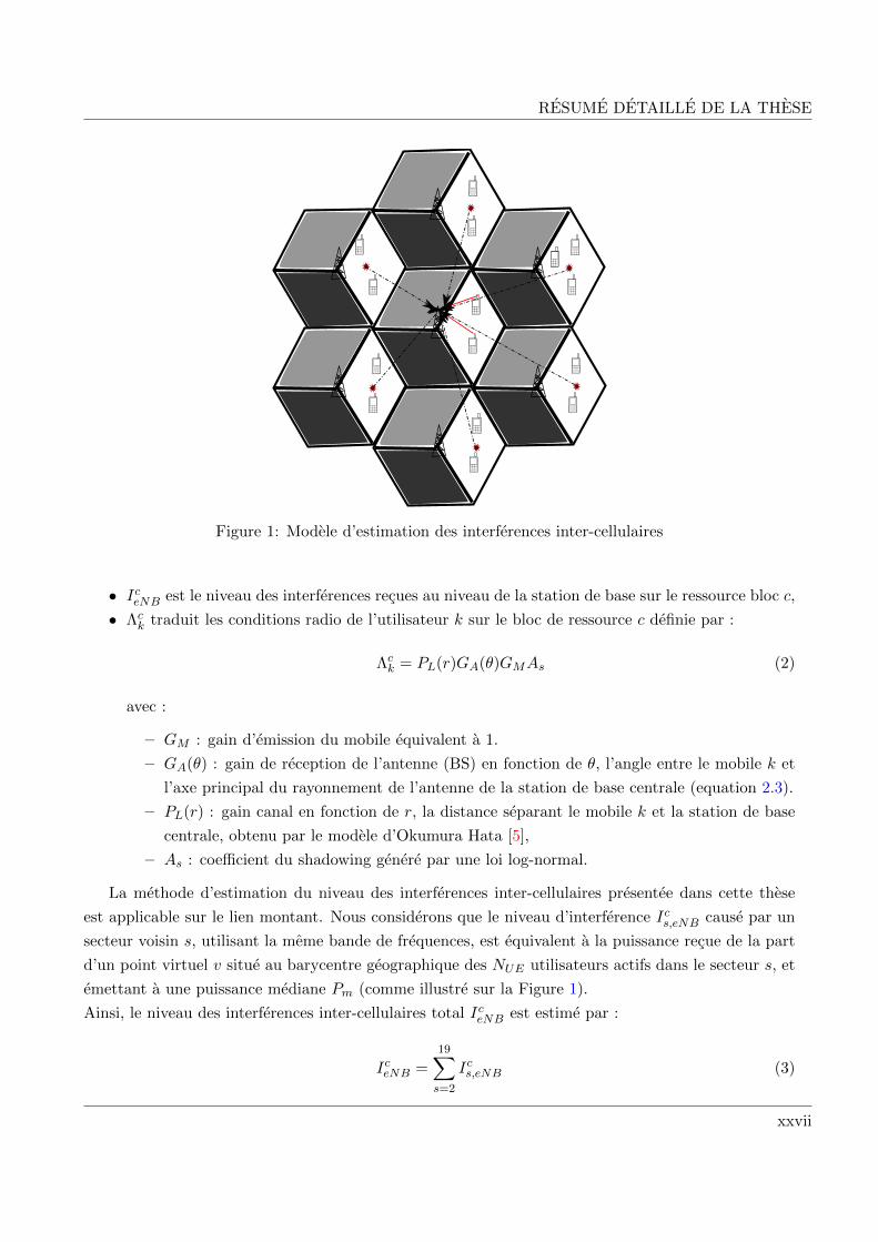
Figure 1: Modele d’estimation des interferences inter-cellulaires
• IceNB est le niveau des interferences recues au niveau de la station de base sur le ressource bloc c,
• Λck traduit les conditions radio de l’utilisateur k sur le bloc de ressource c definie par :
Λck = PL(r)GA(θ)GMAs (2)
avec :
– GM : gain d’emission du mobile equivalent a 1.
– GA(θ) : gain de reception de l’antenne (BS) en fonction de θ, l’angle entre le mobile k et
l’axe principal du rayonnement de l’antenne de la station de base centrale (equation 2.3).
– PL(r) : gain canal en fonction de r, la distance separant le mobile k et la station de base
centrale, obtenu par le modele d’Okumura Hata [5],
– As : coefficient du shadowing genere par une loi log-normal.
La methode d’estimation du niveau des interferences inter-cellulaires presentee dans cette these
est applicable sur le lien montant. Nous considerons que le niveau d’interference Ics,eNB cause par un
secteur voisin s, utilisant la meme bande de frequences, est equivalent a la puissance recue de la part
d’un point virtuel v situe au barycentre geographique des NUE utilisateurs actifs dans le secteur s, et
emettant a une puissance mediane Pm (comme illustre sur la Figure 1).
Ainsi, le niveau des interferences inter-cellulaires total IceNB est estime par :
IceNB =19∑s=2
Ics,eNB (3)
xxvii

RESUME DETAILLE DE LA THESE
Figure 2: Histogramme des puissances de transmission des mobiles apres controle de puissance
Ou :
Ics,eNB = Pm.Λcv‖h‖2 (4)
Nous avons choisi la puissance mediane Pm plutot que la puissance moyenne car en statistique, celle-
ci est plus fiable pour representer la tendance centrale d’une distribution asymetrique [6] [7] [8].
La Figure 2, representant l’histogramme des puissances de transmission des mobiles avec un tirage
aleatoire des interferents dans les secteurs voisins, confirme l’asymetrie de la distribution des puissances
de transmission.
Pour valider la methode proposee, nous comparons ses performances avec celles generees par des
tirages de Monte Carlo. Pour ce faire, nous comparons la distribution des puissances de transmission
des mobiles apres controle de puissance en estimant le niveau des interferences inter-cellulaires avec
la methode proposee, avec la distribution des puissances de transmission apres controle de puissance
lorsqu’on tire aleatoirement un interferent dans chaque secteur voisin. Afin de comparer les deux
distributions, nous utilisons deux tests probabilistes :
1. Le test Log Ratio : defini par le logarithme du rapport entre deux distributions. Dans notre
cas le rapport entre la densite de probabilite des puissances de transmission apres controle de
puissance en estimant le niveau des interferences inter-cellulaires par le modele propose et la
densite de probabilite des puissances de transmission apres controle de puissance en calculant le
niveau des interferences inter-cellulaires avec la methode de Monte Carlo. On note ce rapport
xxviii

RESUME DETAILLE DE LA THESE
∆(x) et on le calcule par la formule suivante :
∆(x) = logProb(dM ≤ x)
Prob(dMC ≤ x)(5)
Nous considerons que le modele d’estimation d’IIC est valide si le logarithme du rapport des
deux distributions ∆(x) est inferieur a 1 ou idealement tant vers 0.
2. Le test de divergence de Kullback-Leibler : plus utilise dans le domaine de la theorie
de l’information, il est considere comme un test Log Ratio pondere. Ce test est une mesure
non-symetrique de la difference entre deux distributions. On le note KL(x) et definit comme
suit :
KL(x) = Prob(dM ≤ x).∆(x) (6)
Pour ces deux tests, dM et dMC representent les puissances de transmission stables des mobiles
(puissance de transmission apres convergence du controle de puissance) obtenues en estimant le
niveau des interferences inter-cellulaires par le modele propose ”Modele d’estimation des IIC”
(Algorithme 1) et par la methode de ”Monte Carlo” (Algorithme 2) respectivement.
Pour des raisons d’equite, nous considerons dans nos simulations que tous les utilisateurs cherchent
a atteindre le meme debit (le meme γtg), et nous n’allouons qu’un seul bloc de ressource a chaque
utilisateur.
Algorithm 1 Modele d’estimation des IIC
Init : Ic = 0Placer aleatoirement NUE utilisateurs actifs,Determiner leur barycentre,for It = 1 to S do
for k = 1 to MS do
P ckTx(It) = min[γtg∗(N+IceNB)
Λck|h|2, Pmax
]end forPm = median[P ckTx ]
IceNB =∑19
k=2 PmΛck|h|2: IIC generee par les 18 secteurs interferentsend forfor k = 1 to MS doPSk = P ckTx(S): puissance de transmission stable de l’utilisateur k
end forVS(i) = [PS1PS2 ...PSMS ]: sauvegarde des puissances d’emission apres controle de puissance.
L’algorithme 1 resume les etapes proposees pour l’estimation du niveau des interferences inter-
cellulaires, avec S le nombre d’iterations necessaires pour la convergence de la puissance d’emission.
La Figure 3 represente la densite de probabilite des puissances de transmission stables des mobiles
dans la cellule centrale en estimant le niveau des interferences par le modele propose et la densite
de probabilite des puissances de transmission stables des mobiles dans la cellule centrale en calculant
xxix

RESUME DETAILLE DE LA THESE
Algorithm 2 Simulation de Monte Carlo
Init : P ckTx = Pmax k = 1, ..., NUE
for i = 1 to M doTirer aleatoirement NUE utilisateurs actifsPour chaque utilisateur actiffor m = 1 to MT do
Tirer aleatoirement un utilisateur interferent ks dans chaque secteur voisin s avec une puissancede transmission P ckTx,sfor It = 1 to S do
for s = 2 to 19 doIceNB =
∑19s=2 P
ckTx
Λck|h|2 .end forP ckTx(It) = min[
γtg∗(N+IceNB)
Λck|h|2, Pmax], mise a jour de P ckTx pour k = 1, ..., NUE .
end forPSk = P ckTx(S), Puissance de transmission stableVS(m) = [PS1 , PS2 , ..., PSMT
]end forSauvegarder VS(m) dans la matrice Mat P(i) M ×NUE
end forSauvegarder Mat P (i) dans la table de resultats (Taille finale : (MT ∗M)×NUE).
le niveau des interferences par la methode de Monte Carlo. Nous remarquons la similitude des deux
courbes obtenues par les deux approches. La puissance de transmission stable des mobiles varie entre
−48 dBm et 21 dBm. Cette plage de variation respecte l’intervalle exige par la norme [9]. Le tableau 1
represente les resultats de simulation obtenues par le test Log Ratio dans le cas :
• PL : Attenuation de parcours (Path Loss) uniquement en utilisant le modele d’Okmura Hata.
• PL+Fad : Attenuation de parcours avec un fading de Rayleigh d’ecart-type σf = 1.
• PL+Fad+Shad : Attenuation de parcours avec un fading de Rayleigh d’ecart-type σf = 1 et un
Shadowing d’ecart-type σs = 4 dB.
Les valeurs resumees dans le tableau sont tres inferieures a 1. La plus grande valeur de ∆(x) est egale
a 0.14, ce qui nous permet de valider notre modele.
La Figure 4 represente le resultat obtenu par le test de divergence de Kullback-Leibler. La courbe
representant KL(x) dans le cas considerant le modele d’Okumura Hata uniquement presente un max-
imum de 0.03. Pour tester la robustesse du modele nous avons ajoute du fading de Rayleigh et du
shadowing avec differents ecart-types. Nous avons fait varier l’ecart-type du fading de Rayleigh (σf )
de 1 a 3, et l’ecart-type du shadowing (σs) de 4 dB a 7 dB. Les courbes representant le test Kullback-
Leibler avec ces variations de parametres sont plus lisses et avec une dynamique plus importante.
Mais dans tous les cas de figures, les valeurs respectent la condition de validite du test Log Ratio (le
maximum atteint est 0.1 avec un fading de Rayleigh d’ecart-type σf = 1 et un shadowing d’ecart-type
de σs = 7 dB).
xxx

RESUME DETAILLE DE LA THESE
Puissance (dBm)∆(x)
σf =1, σs = 4 dBPL PL + Fad PL+Fad+Shad
≤ -30 0.14 0.11 0.122
[-30;-25] 0.048 0.063 0.11
[-25;-20] 0.04 0.009 0.099
[-20;-15] 0.024 0.026 0.09
[-15;-10] 0.022 0.033 0.078
[-1;-5] 0.02 0.024 0.068
[-5;0] 0.03 0.042 0.06
[0;5] 0.043 0.042 0.049
[5;10] 0.026 0.031 0.037
[10;15] 0.014 0.018 0.0 28
[15;21] 0.003 0.0042 0.015
Table 1: Le test Log Ratio ∆(x)
−50 −40 −30 −20 −10 0 10 200
0.1
0.2
0.3
0.4
0.5
0.6
0.7
0.8
0.9
1
Transmission power (dBm)
Pro
ba
bili
ty (
Psj<
=x)
Proposed method
Monte Carlo draws
Figure 3: Densite de probabilite des puissances de transmission des mobiles apres convergence
xxxi

RESUME DETAILLE DE LA THESE
−100 −80 −60 −40 −20 0 20 400
0.01
0.02
0.03
0.04
0.05
0.06
0.07
0.08
0.09
0.1
Power (dBm)
Ku
llba
ck−
Le
ible
r d
ive
rge
nce
te
st
σf
=1, σs
=7
σf
=1, σs
=4
Path loss
σf
=2, σs
=4
σf=3, σ
s=4
σf
=1, σs
=5
σf
=1, σs=6
Figure 4: Le test de divergeance de Kullback-Leibler
Afin de valider le modele analytiquement et tester la fiabilite de la puissance mediane Pmed par
rapport a la puissance moyenne Pmean, nous avons developpe l’expression analytique de Pmed et Pmean.
La validite du modele analytique a ete prouvee grace aux tests statistiques utilises lors de la simulation.
De la Figure 5, nous constatons la validite du modele puisque les valeurs du test de Kullback-Leibler
obtenues sont faibles, et la meilleure performance est obtenue par le modele utilisant la puissance
mediane.
Chapitre 4 - Modele analytique de la borne superieure de la probabilite de depassement
de dimensionnement
Sachant que le nombre de blocs de ressources dans une bande de frequences est limite, l’entite re-
sponsable de l’allocation des ressources radio cherche a maximiser les performances du reseau en
allouant efficacement les RBs aux utilisateurs. Cet objectif ne peut etre atteint que lorsque la bande
de frequences allouee a une cellule est adaptee a sa charge ainsi qu’a la QdS offerte aux utilisateurs.
Dans cette these, nous avons developpe un modele analytique qui permet d’evaluer la borne superieure
de la probabilite de depassement de dimensionnement et ce, en fonction de la charge du reseau, de
la QdS offerte aux utilisateurs et de la politique d’allocation de RB appliquee. Nous avons considere
une politique d’allocation equitable et opportuniste dans un systeme SISO et un systeme MIMO,
lorsqu’une ou plusieurs QdS sont offertes aux utilisateurs.
Nous considerons qu’une cellule est en depassement de dimensionnement, lorsque cette derniere
n’a pas assez de blocs de ressources pour les allouer aux utilisateurs qui lui sont rattaches en satis-
xxxii

RESUME DETAILLE DE LA THESE
−40 −30 −20 −10 0 10 20 300
0.02
0.04
0.06
0.08
0.1
0.12
0.14
0.16
0.18
UE Transmission power (dBm)
Kullb
ack−
Leib
ler
test
Proposed method with median
Proposed method with mean
Figure 5: Test de divergence de Kullback-Leibler entre le modele analytique de la methode proposeeet le tirage de Monte Carlo
.
faisant leur QdS. Afin de developper le modele analytique de la borne superieure de la la probabilite
de depassement de dimensionnement, nous utilisons la geometrie stochastique et son large arsenal
d’outils mathematiques.
On considere NUE = |ϕUE | le nombre d’utilisateurs presents dans la cellule C et ϕUE l’ensemble
de ces utilisateurs. Le debit correspondant a la QdS requise par l’utilisateur est note C0. Le nombre
total de RBs N necessaires pour servir et satisfaire la QdS de tous les utilisateurs presents dans la
cellule C est donc:
N =∑
k∈ϕUE
Nk(x) (7)
avec Nk(x) le nombre total de RBs necessaires pour satisfaire la QdS de l’utilisateur k.
Nous considerons que le systeme est en depassement de dimensionnement, si le nombre total de RB
necessaires pour servir et satisfaire la QdS de tous les utilisateurs de la cellule N est superieur au
nombre de RBs disponibles au niveau de la station de base.
Lors de l’etablissement du modele analytique de la borne superieure de la probabilite de depassement
de dimensionnement, nous avons calcule les debit en fonction de la capacite de Shannon. Ainsi, le
xxxiii

RESUME DETAILLE DE LA THESE
nombre de RB necessaires pour satisfaire la QdS de l’utilisateur k est :
Nk =
⌈C0
Ck
⌉(8)
avec Ck = W log2(1 + γk) la capacite de Shannon moyenne, W la largeur de bande de frequences d’un
RB et γk le niveau du SINR permettant d’atteindre la QdS requise par l’utilisateur k.
Afin de simplifier les calculs, nous avons pose les hypotheses suivantes:
1. La cellule C est ronde, d’un rayon R, avec une station de base munie d’une antenne omnidi-
rectionnelle situee au centre de la cellule
2. On n’autorise un utilisateur a transmettre que si :
- le niveau de SINR de l’utilisateur est superieur a γmin, ce qui implique un nombre maxi-
mum de RBs Nmax a allouer a un utilisateur, donne par :
Nmax =
⌈C0
W log2(1 + γmin)
⌉(9)
- l’utilisateur est selectionne par l’ordonnanceur (i.e. z = 1 ou z = 0 indique respective-
ment si l’utilisateur est selectionne ou pas par l’ordonnanceur). Deux types de politique
d’allocation de ressources radio sont consideres :
(a) une politique equitable : tous les utilisateurs ont la meme chance d’etre selectionnes
par l’ordonnaceur,
(b) une politique opportuniste : l’ordonnanceur selectionne en premier l’utilisateur ayant
les meilleures conditions radio.
3. Le controle de puissance de transmission des utilisateurs n’est pas pris en compte. Ainsi, la
puissance de transmission moyenne d’un utilisateur par RB est PkTx = PmaxNmax
.
En se basant sur ces hypotheses, nous developpons un modele analytique de la borne superieure de
la probabilite de depassement de dimensionnement en considerant une politique d’allocation equitable
et opportuniste dans un systeme SISO et MIMO avec une et plusieurs QdS.
Borne superieure de la probabilite de depassement de dimensionnement dans un
systeme SISO
La probabilite de depassement de dimensionnement est donnee par :
Pout = Prob
(∫Ndϕ ≥ NRB
)(10)
En se basant sur la geometrie stochastique, ou les utilisateurs sont generes par un processus de Poisson
ponctuel d’intensite Λ(x) (donne en fonction de la densite surfacique des utilisateurs ρ et leur temps
moyen de service ν, Λ(x) = ρν ), nous utilisons le theoreme de la limite centrale (theoreme 2.3) pour
calculer la borne superieure de la probabilite de depassement de dimensionnement. Lorsque αNRB
xxxiv

RESUME DETAILLE DE LA THESE
blocs de ressources sont alloues a la cellule, la borne superieure de la probabilite de depassement de
dimensionnement Psup est exprimee par:
Prob
(∫Ndϕ ≥ αNRB
)≤ Psup
ou,
Psup = exp(− vNN2
maxg(
(α−1)mNNmax
vN
))(11)
avec g(t) = (1 + t) ln(1 + t)− t.
Pour obtenir Psup, nous devons calculer les deux premiers moment mN et vN de notre processus.
Le nombre de RB necessaires pour satisfaire la QdS de chaque utilisateur k est :
Nk(x, y, z) =
⌈C0
W log2
(1+
PtPL(x)
ηy
)⌉z (12)
=
C0
W log2
(1+
PtK
ηy‖x‖β
) z
(13)
Le processus de Poisson ponctuel est donc marque par la marque du shadowing note y et la marque
de la decision de l’ordonnanceur z. Ces marques etant independantes, le processus de Poisson marque
devient un processus de Poisson ponctuel dans R3 d’intensite Λ(x)⊗ ps(y)dy ⊗ p(z)dz.Grace a la formule de Campbell (Formule 2.1) nous pouvons calculer mN et vN comme suit:
mN =
∫N(x, y, z) ps(y)dy p(z)dz dΛ(x) (14)
et
vN =
∫N2(x, y, z) ps(y)dy p(z)dz dΛ(x) (15)
Les deux premiers moments du processus N peuvent aussi etre exprimes en fonction des aires Aj
contenant les utilisateurs ayant besoin au plus de j RBs pour satisfaire leur QdS :
mN =ρ
ν
Nmax−1∑j=1
j(Aj −Aj−1) +ρ
νNmax(πR2 −ANmax−1) (16)
et
vN =ρ
ν
Nmax−1∑j=1
j2(Aj −Aj−1) +ρ
νN2
max(πR2 −ANmax−1) (17)
xxxv

RESUME DETAILLE DE LA THESE
On considere γj le seuil du niveau du SINR, j le nombre de RBs necessaires a l’utilisateur pour
atteindre sa QdS definie par son debit cible C0, avec :
γj = 2C0/(jW ) − 1 pour j = 1, · · · , Nmax − 1 et γ0 =∞
Les surfaces Aj peuvent etre determines par :
Aj =
∫C×R+×Z
1y‖x‖β≤PtK/ηγj ps(y)dy p(z)dz dx
=
∫C×R+×Z
p(y‖x‖β ≤ γj
)p(z)dz dy dx (18)
avec γj = PtKηγj
.
Dans le cas d’une allocation equitable de RBs, nous obtenons :
Aj = νρR2 exp (2/ζ + 2αj/ζ)Φ(ζ lnR− 2/ζ − αj) + ν
ρΦ(αj − ζ lnR) (19)
Lorsqu’une allocation opportuniste de RB est utilisee, nous obtenons :
Aj = 2π
∫ R
0
1−(
1− Φ( γjrβ− µsσs
))NUE r dr (20)
Lorsque plusieurs QdS sont offertes aux utilisateurs, nous considerons chaque classe d’utilisateurs
demandant une QdS definie comme etant un processus de Poisson ponctuel marque par sa classe de
QdS l, avec l ∈ L. Le developpement du modele analytique de la borne superieure de la probabilite
de depassement de dimensionnement de tout le systeme, considerant les differentes QdS offertes reste
inchange. La difference reside dans le calcul des deux premiers moments du processus global qui
peuvent etre decrits comme suit :
mN =∑L
l=1mN,l (21)
vN =∑L
l=1 vN,l, (22)
et la valeur du nombre maximum de RBs alloues a un utilisateur est definie par :
Nmax = maxl
Nl,max (23)
Ainsi, la borne superieure de la probabilite de depassement de dimensionnement P SISOsup,QoS est donnee
par :
P SISOsup,QoS = exp
(− vNN2
maxg(
(α−1)mN Nmax
vF
))(24)
xxxvi

RESUME DETAILLE DE LA THESE
Borne superieure de la probabilite de depassement de dimensionnement dans un
systeme MIMO
Dans le cas d’un systeme MIMO, pour des raisons de complexite de calcul, nous ne considerons que
l’effet du fading. Le signal venant d’un meme utilisateur subit la meme attenuation de parcours et
le meme shadowing. Ce qui differencie la qualite du signal venant des differentes antennes d’emission
d’un meme mobile sont les differentes coefficients du fading subi sur chacun des chemins. Dans ce
systeme, nous avons etudie le gain de diversite et le gain de multiplexage.
1- Gain de diversite
Il consiste a choisir le meilleur chemin pour envoyer l’information. Lorsque une politique d’allocation
equitable est consideree, cela revient a une selection aleatoire de l’utilisateur qui transmet, mais le
choix de l’antenne de transmission se fait sur la base des coefficients des fading qu’il subit sur les
differents chemins. Considerons nt antennes de transmission et nr antennes de reception, le chemin
choisi est |h∗|2, qui maximise le gain de fading sur ntnr chemins.
|h∗|2 = max1≤i≤nt,1≤j≤nr
|hi,j |2.
En appliquant les meme etapes de developpement utilisees dans le cas d’un systeme SISO, nous
obtenons la borne superieure de la probabilite de depassement de dimensionnement en fonction
des deux premiers moments du processus. Ces derniers se calculent en fonction des aires Aj dont
l’expression dans le cas d’un systeme MIMO avec gain de diversite utilisant une politique d’allocation
de RB equitable est :
Aj = 1NUE
[πR2 − 2π
∫ R
0r
(1− e−
rβ
γj
)ntnrdr
](25)
Lorsque une politique d’allocation de RB opportuniste est utilisee, l’utilisateur selectionne par l’ordonnanceur
est celui qui a les meilleurs conditions radio, et la transmission se fait sur le meilleur chemin. Ceci
revient a choisir l’utilisateur ayant le meilleur gain de fading parmi NUE utilisateurs et le meilleur
coefficient de fading parmi ntnr chemins :
k∗ = arg max1≤k≤NUE
[max
1≤i≤nt,1≤j≤nr| h(k)
i,j |2].
L’expression de Aj dans ce cas la est donnee par :
Aj = πR2 − 2π
∫ R
0r
(1− e−
rβ
γj
)NUEntnr
dr (26)
xxxvii

RESUME DETAILLE DE LA THESE
2- Gain de multiplexage
Cette technique consiste a transmettre l’information sur les nt antennes de transmission. On suppose
que les conditions canal ne sont pas connues de l’emetteur. La puissance de transmission est repartie
equitablement sur ses nt antennes. La capacite du canal depend donc des valeurs propres de la
matrice HH† = UDU†. D est la matrice diagonale contenant les valeurs propres µ1, µ2, . . . , µm de la
decomposition de HH† avec m = min(nt, nr). Dans ce cas, la capacite du MIMO est decrite comme
suit,
C = log2 det(Int + PtK
ntη‖x‖βHH†)
(27)
= C log2
∏mi=1
(1 + PtKµi
ntη‖x‖β
)(28)
En considerant Ctot le debit total exige par un utilisateur afin qu’il puisse transmettre les flux de
donnees sur les nt antennes, le nombre de RB necessaires afin de satisfaire la QdS de cet utilisateur
est donc :
Nk(x, µ, z) =
Ctot
W log2(∏mi=1(1 + PtKµi
ntη‖x‖β ))
z (29)
Les valeurs propres n’etant pas independantes, nous avons ete contraints de faire le dimensionnement
sur une seule antenne. Pour des raisons evidentes nous avons prefere un sur-dimensionnement du
reseau prenant en compte l’antenne necessitant le plus de RBs (i.e. ayant la plus petite valeur propre).
Puisque les valeurs propres sont ordonnees, le nombre necessaire de RBs pour satisfaire la QdS de
l’utilisateur k est :
Nk(x, µ, z) ≥
Ctot
Wm log2
(1 + PtKµ1
ntη‖x‖β
) z (30)
Lorsqu’une politique d’allocation de RB equitable est utilisee, l’utilisateur selectionne par l’ordonnanceur
est choisi aleatoirement. En revanche, le dimensionnement se fait sur la plus petite valeur propre µ1
comme decrit precedemment. Les deux premier moments du processus sont calcules en fonction des
aires Aj , dont l’expression dans un systeme MIMO 2x2 est donnee par :
Aj = 1NUE
[πR2 − 2π
∫ R
0
(1− e
−2 rβ
γMIMOj
)rdr
](31)
Dans le cas d’une politique d’allocation opportuniste, l’utilisateur choisi est celui beneficiant des
meilleures conditions radio et le dimensionnement se fait toujours sur la plus petite valeur propre.
L’expression de Aj est donc donnee par :
Aj = πR2 − 2π
∫ R
0
(1− e
−2 rβ
γMIMOj
)NUE
rdr, (32)
xxxviii

RESUME DETAILLE DE LA THESE
1.3 1.4 1.5 1.6 1.7 1.80
0.05
0.1
0.15
0.2
0.25
0.3
0.35
0.4
0.45
α
∆F
air
SIS
O=
log(P
sup,F
air
SIS
O/P
out,F
air
SIS
O)
∆Fair,100 kbps
SISO
∆Fair,200 kbps
SISO
∆Fair,300 kbps
SISO
∆Fair,400 kbps
SISO
Figure 6: Test Log Ratio de la borne superieure de la probabilite de depassement de dimensionnementdans un systeme SISO avec une politique equitable d’allocation de RB
Afin de valider le modele, nous avons utilise le test Log Ratio defini precedement. Ce test permet de
mesurer l’ecart entre la borne superieure de la probabilite de depassement de dimensionnement obtenue
par le modele analytique propose, et la probabilite de depassement de dimensionnement obtenue par
simulation par des tirages de Monte Carlo. Les resultats obtenus (Figure 6 dans le cas d’un systeme
SISO et Figure 7 dans le cas d’un systeme MIMO) nous ont permis de valider le modele dans le cas de
systemes SISO et MIMO avec gain de multiplexage et gain de diversite, tout en considerant les deux
types de politique d’allocation de RB.
La borne superieure de la probabilite de depassement de dimensionnement nous a permis de juger
si la bande de frequences allouee est adequate ou non au reseau tout en considerant la charge du reseau,
la QdS offerte, la politique d’allocation de RB adoptee et le systeme utilise. Dans le cas ou la bande
de frequences est non adequate (probabilite de depassement elevee), nous proposons d’accroıtre le
nombre de RBs disponibles en augmentant la bande allouee au reseau avec la technique d’aggregation
de porteuse (Carrier Aggregtion). Ceci nous permet d’augmenter le nombre total de RBs dans la
cellule et de diminuer par la meme occasion la probabilite de depassement de dimensionnement.
xxxix

RESUME DETAILLE DE LA THESE
1.3 1.4 1.5 1.6 1.7 1.80.26
0.28
0.3
0.32
0.34
0.36
0.38
0.4
0.42
0.44
c
Log r
atio test
∆Opp
Div,MIMO
∆Fair
Mux,MIMO
∆Opp
Mux,MIMO
∆Fair
Div,MIMO
Figure 7: Test Log Ratio de la borne superieure de la probabilite de depassement de dimensionnementdans un systeme MIMO
Chapitre 5 - Allocation des ressources radio
Apres avoir defini la bande de frequences adequate a allouer a une cellule, nous nous interessons
ensuite a la politique d’allocation des ressources radio, en nombre limite, aux utilisateurs. Notre objec-
tif est de maximiser le debit total de la cellule. Nous proposons un nouvel algorithme, Opportunistic
and Efficient RB allocation algorithm (OEA), base sur une politique opportuniste, tout en allouant
efficacement les ressources radio (blocs de ressources et puissance de transmission des mobiles) aux
utilisateurs. La solution de l’allocation des ressources radio sur le lien montant est SRB ∈ S qui
maximise la somme des debits individuels des utilisateurs Rk ∀ k = 1, · · · , NUE , avec S l’ensemble
des allocations possibles de RB aux utilisateurs. Le probleme d’allocation des ressources radio sur le
lien montant est donc exprime par:
SRB = arg maxSRB∈S
NUE∑k=1
Rk
sous les contraintes suivantes :
- Chaque RB est alloue exclusivement a un utilisateur,∑k∈K
wck(t) = 1 ∀c ∈ C
xl

RESUME DETAILLE DE LA THESE
avec K l’ensemble des utilisateurs dans la cellule, C l’ensemble des RBs et wck(t) = 0 ou wck(t) = 1
indique si le RB c est alloue a l’utilisateur k a l’instant t.
- Contrainte de contiguıte : les RBs alloues a un meme utilisateur doivent etre contigus dans le
domaine frequentiel,
∀ k ∈ K, wck(t) = 0 ∀ c ≥ j + 2 si wjk(t) = 1 and wj+1k (t) = 0
- Contrainte du MCS robuste : un utilisateur doit utiliser le meme schema de codage et de
modulation (MCS : Modulation and Coding Scheme) sur l’ensemble des RBs qui lui sont allouees
Rk(t) = rk(t)|Ak| (33)
avec Rk(t) le debit total de l’utilisateur k a l’instant t, rk(t) le debit instantane de l’utilisateur
k sur un RB en considerant la contrainte du MCS robuste, et Ak l’ensemble des RB alloues a
l’utilisateur k.
- Prise en compte de la limite de la puissance de transmission du mobile, puisque la somme des
puissances de transmission d’un meme utilisateur sur les differents RBs qui lui sont alloues ne
doit pas exceder Pmax.
Vu la complexite de l’allocation conjointe (allouer conjointement les RBs et la puissance de trans-
mission), nous avons opte pour une allocation separee. Sachant que le SINR depend de la puissance
de transmission des mobiles, nous avons donc choisi d’allouer dans un premier temps les RBs aux
utilisateurs, puis d’ajuster la puissance de transmission des mobiles en fonction des conditions radio
de chaque l’utilisateur sur les RBs qui lui sont alloues.
L’allocation des RBs prend en consideration les contraintes imposees par la technique SC-FDMA
(i.e. contrainte de contiguıte des RBs et la contrainte du MCS robuste).
L’efficacite de l’algorithme resulte des conditions supplementaires imposees lors de l’allocation
d’un RB supplementaire. L’algorithme propose n’alloue un RB supplementaire a l’utilisateur k que
si l’allocation de ce dernier ameliore le debit total de l’utilisateur tout en respectant la contrainte du
MCS robuste.
En SC-FDMA la puissance de transmission du mobile est equitablement repartie sur l’ensemble des
RBs alloues a un utilisateur. Puisque le SINR efficace sur un RB depend de la puissance de transmission
du mobile sur ce meme RB, une mise a jour de la metrique (i.e. SINR) est donc appliquee avant chaque
nouvelle allocation, telle que :
γeff(k,c) = γeff
(k,c) − 10 log(|Ak|+ 1) ∀c ∈ Ak (34)
avec γeff(k,c) le SINR efficace moyen de l’utilisateur k sur RB c, et |.| la cardinalite d’un ensemble.
Une condition supplementaire est verifiee lors de l’extension de l’allocation. Cette derniere impose
xli

RESUME DETAILLE DE LA THESE
un nombre maximum de RB alloues a un utilisateur αkmax . Dans le cas opportuniste, un nombre
maximum egal au nombre maximum de RBs dans la cellule, est autorise (i.e. la station de base peut
allouer a un meme utilisateur tous les RBs dont elle dispose αkmax = NRB).
Afin d’adapter cet algorithme a la QdS des utilisateurs, une variante de l’algorithme, nommee QoS
based OEA, est proposee. Cette variante fixe le nombre maximum de RBs a allouer a un utilisateur
en fonction de sa QdS demandee (definie par Rtarget,k le debit cible de l’utilisateur k) et ses conditions
radio tel que :
αkmax =
⌈Rtarget,krk(t)
⌉(35)
L’allocation des RBs aux utilisateurs considere que la puissance de transmission des mobiles est
fixee a Pmax. A la fin du processus d’allocation de RB, l’utilisateur k atteint un debit Rk(t). Notre
objectif est de diminuer la puissance de transmission Pe,k du mobile k en appliquant un controle de
puissance, sans affecter son debit atteint avant le controle de puissance. Pour atteindre cet objectif,
le controle de puissance doit prendre en compte le niveau minimum du SINR, atteint sur l’ensemble
des RBs allouees, afin de garantir l’utilisation du meme MCS qu’avant le controle de puissance. Ainsi
le controle de puissance est defini dans ce cas par :
Pe,k =Pmax
|Ak|γtg
γeff(k,min)
(36)
ou, γtg le debit cible est exprime en dB comme suit :
(γtg)dB = (γMCS,k)dB + (∆γ)dB (37)
avec γMCS,k le niveau minimum du SINR requis pour pouvoir utiliser le meme MCS, ∆γ une marge
de SINR, et γeff(k,min) le SINR minimum effectivement atteint par l’utilisateur k sur l’ensemble des RBs
qui lui sont alloues :
γeff(k,min) = min
c∈Akγeff
(k,c) (38)
Les performances de l’algorithme propose sont etudiees dans un reseau regulier (i.e. compose
de cellules hexagonales, chacune munie d’une station de base au centre de la cellule) et un reseau
aleatoire (i.e. un reseau genere par la superposition de deux processus de Poisson d’intensite λeNB
et λUE representant respectivement les stations de base et les utilisateurs) en termes de complexite,
debit agrege, efficacite energetique, nombre d’utilisateurs servis, taux de RBs alloues et equite de debit
entre les utilisateurs.
Les performances du OEA sont comparees avec les performances de la methode optimale obtenue
par la programmation entiere [10], connue pour sa complexite, et d’autres algorithmes references
xlii

RESUME DETAILLE DE LA THESE
0 50 100 150 2000
0.5
1
1.5
2
2.5
3
3.5
4
4.5
5x 10
5
Number of users
Num
ber
of oppera
tions
OEA
RME
FDPS−LMF
HLGA
Figure 8: Nombre d’opaerations necessaires pour l’allocation des ressources radio
dans le domaine tels que : Frequency Domain Packet Scheduling- Largest Mertic First (FDPS-LMF),
Recursive Maximum Expansion (RME), Heuristic Localized Gradian Algorithm (HLGA), proposes
respectivement dans [11], [12] et [13].
La complexite etant polynomiale pour les algorithmes OEA, FDPS-LMF, HLGA et RME, nous
avons calcule et compare le nombre necessaire d’operations a effectuer par chacun des algorithmes
pour allouer les RBs aux utilisateurs de la cellule, et ce pour differentes charges du reseau. La Fig-
ure 8 montre que le nombre d’operations necessaires pour l’algorithme OEA est inferieur a celui de
l’algorithme RME lorsque le nombre d’utilisateurs dans la cellule depasse 70 utilisateurs. Le nombre
d’operations necessaires pour allouer les RBs aux utilisateurs, lorsqu’une bande de 10 MHz est allouee
a la cellule et que le nombre d’utilisateurs NUE est egal a 100, est inferieur a 0.2 million operations.
Ceci prouve que l’algorithme peut etre execute en moins de 0.5 ms (la periode d’ordonnancement) avec
une station de base munie d’un processeur a deux corps qui operent a 2 x 34 k millions d’instructions
par seconde (disponible dans le marche).
La Figure 9 illustre les debits agreges obtenus par les differents algorithmes. Le debit agrege
obtenu par l’OEA est proche de celui obtenu par la methode optimale. L’algorithme QoS based OEA
atteint un debit agrege un peu plus faible. Ceci est du au debit cible exige par les utilisateurs fixe a
600 kbps. Les algorithmes HLGA, FDPS-LMF et RME atteignent le plus faible debit agrege car leur
metrique cherchant une equite en debit entre les utilisateurs, ils allouent les RBs aux utilisateurs qui
xliii

RESUME DETAILLE DE LA THESE
ont un faible debit et probablement des conditions radio qui ne leur permettent finalement meme pas
d’employer le plus robuste des MCS.
0 0.5 1 1.5 2 2.5 3 3.5
x 10−4
0
1
2
3
4
5
6
7
8
9
10
λUE
Agg
reg
ate
th
rou
gh
pu
t (M
bp
s)
RME
FDPS
HLGA
QoS based OEA
Optimal
Optimal−es
Opport
OEA
Figure 9: Debit agrege dans un secteur d’un reseau aleatoire
La Figure 10 represente la proportion d’utilisateurs servis par chaque algorithme. L’algorithme
QoS based OEA, avec ses conditions de debit ameliore et de nombre maximum de RBs alloues par
utilisateur, permet de maximiser la proportion d’utilisateurs servis. Les algorithmes HLGA et FDPS-
LMF atteignent une proportion d’utilisateurs servis elevee. Ceci est du a leur politique d’allocation
qui considere qu’un utilisateur est servi lorsque l’expansion de l’allocation est interrompue a cause
de la contrainte de contiguite non satisfaite entre les RBs ou l’utilisateur en question maximise la
metrique.
Les algorithmes RME, FDPS-LMF et HLGA, allouant des RBs a des utilisateurs ne pouvant pas
employer le plus robuste des MCS, atteignent un debit nul quelque soit le nombre de RBs qui leur est
alloue. Ils maximisent donc le taux de RBs gaspilles (i.e. allouer des RBs a des utilisateurs ayant un
debit nul). La Figure 11 presentant le taux moyen de RBs gaspilles montre que les algorithmes OEA
et QoS based OEA annulent le gaspillage des RBs grace a la mise a jour de la metrique avant chaque
nouvelle allocation et leur condition d’amelioration de debit.
xliv

RESUME DETAILLE DE LA THESE
0 0.5 1 1.5 2 2.5 3 3.5
x 10−4
0
0.1
0.2
0.3
0.4
0.5
0.6
0.7
0.8
0.9
1
λUE
Avera
ge p
roport
ion o
f serv
ed U
E
RME
FDPS
HLGA
QoS based OEA
Optimal
Optimal−es
Opport
OEA
Figure 10: Proportion moyenne d’utilisateurs servis dans un reseau aleatoire
0 0.5 1 1.5 2 2.5 3 3.5
x 10−4
0
0.1
0.2
0.3
0.4
0.5
0.6
0.7
0.8
0.9
λUE
Avera
ge r
atio o
f w
aste
d R
Bs
RME
FDPS
HLGA
QoS based OEA
Optimal
optimal−es
Opport
OEA
Figure 11: Taux moyen de RB gaspilles dans un reseau aleatoire
xlv

RESUME DETAILLE DE LA THESE
0 1 2 3 4
x 10−4
0
0.1
0.2
0.3
0.4
0.5
0.6
0.7
0.8
0.9
1
λUE
Fairness in term
of T
hro
ughput
RME
FDPS
HLGA
QoS based OEA
Optimal
Optimal−est
Opport
OEA
Figure 12: Equite en terme de debit entre les utilisateurs dans un reseau aleatoire
Nous avons calcule l’equite en terme de debit comme definie dans [14], et donnee par :
FAlg =
(∑NUEk=1 Rk(∆T )
)2(NUE
∑NUEk=1 Rk(∆T )2
) (39)
La Figure 12 illustrant cette equite montre que les algorithmes RME, FDPS-LMF et HLGA max-
imisent l’equite en terme de debit entre les utilisateurs. Le calcul d’equite de ces algorithmes prend
cependant en compte les utilisateurs ayant un debit nul. Vu le taux de gaspillage de RB observe pour
ces algorithmes, nous soupconnons que ce niveau eleve d’equite est aussi du au taux eleve de RB
gaspilles.
En terme d’efficacite energetique, nous avons compare le niveau moyen de puissance de transmission
des utilisateurs apres le controle de puissance. La Figure 13 montre que la puissance de transmission
moyenne atteinte par les algorithmes proposes, a forte charge, est de 13 dBm. Cette reduction de
puissance de transmission des mobiles permet de maximiser l’efficacite energetique et de maximiser la
dure de vie de la batterie des mobiles.
Chapitre 6 - Allocation des RBs dans une systeme multi-utilisateurs
Vu les performances de l’algorithme propose OEA, nous avons etendu l’etude de ce dernier dans
un systeme multi-utilisateurs MIMO (MU-MIMO), ou plusieurs utilisateurs potentiels Nu,p peuvent
transmettre leurs donnees dans un meme RB, grace a un codeur/ decodeur adapte. Pour cela, nous
xlvi

RESUME DETAILLE DE LA THESE
0 0.5 1 1.5 2 2.5 3 3.5
x 10−4
12
13
14
15
16
17
18
19
20
21
λUE
UE
s tra
nsm
issio
n p
ow
er
(dB
m)
Pmax
QoS based OEA
OEA
Opportunistic
Optimal
Optimal−es
RME
HLGA
FDPS−LMF
Figure 13: Puissance de transmission moyenne des utilisateurs sur un TTI, dans un reseau aleatoire
proposons un nouveau decodeur (Figure 14) qui combine un decodeur zero forcing (ZF) et un decodeur
a maximum de vraisemblance (ML) afin d’annuler le niveau d’interference entre utilisateurs partageant
le meme RB et decoder les donnees envoyees par chacun.
.
..
...Multi User
ZF
Single User
Single User
ML
ML
.
..
yeNB
y1
yK
r1 data streams
rK data streams
Figure 14: Decoder combine ZF et ML
Nous avons etudie l’impact de la metrique sur l’algorithme dans un contexte multi-utilisateurs, en
etudiant les performances suivant deux metriques :
• Mrate : maximise le debit par RB. Le nombre d’utilisateurs partageant un RB estNs ≤ min (nr, Nu,p).
• MUE : maximise le nombre d’utilisateurs transmettant des donnees par RB,Ns = min(nr, Nu,p).
Ces deux metriques nous permettent de selectionner les utilisateurs partageant le meme RB.
L’extension de l’allocation des RBs pour chaque utilisateur se fait en fonction de l’algorithme Cen-
xlvii
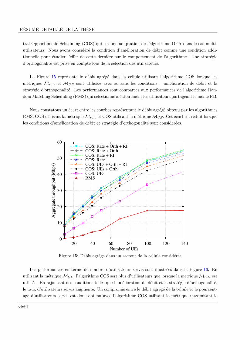
RESUME DETAILLE DE LA THESE
tral Opportunistic Scheduling (COS) qui est une adaptation de l’algorithme OEA dans le cas multi-
utilisateurs. Nous avons considere la condition d’amelioration de debit comme une condition addi-
tionnelle pour etudier l’effet de cette derniere sur le comportement de l’algorithme. Une strategie
d’orthogonalite est prise en compte lors de la selection des utilisateurs.
La Figure 15 represente le debit agrege dans la cellule utilisant l’algorithme COS lorsque les
metriques Mrate et MUE sont utilisees avec ou sans les conditions : amelioration de debit et la
strategie d’orthogonalite. Les performances sont comparees aux performances de l’algorithme Ran-
dom Matching Scheduling (RMS) qui selectionne aleatoirement les utilisateurs partageant le meme RB.
Nous constatons un ecart entre les courbes representant le debit agrege obtenu par les algorithmes
RMS, COS utilisant la metriqueMrate et COS utilisant la metriqueMUE . Cet ecart est reduit lorsque
les conditions d’amelioration de debit et strategie d’orthogonalite sont considerees.
0
10
20
30
40
50
60
20 40 60 80 100 120 140
Ag
gre
gat
e th
rou
gh
pu
t (M
bp
s)
Number of UEs
COS: Rate + Orth + RICOS: Rate + OrthCOS: Rate + RICOS: RateCOS: UEs + Orth + RICOS: UEs + OrthCOS: UEs RMS
Figure 15: Debit agrege dans un secteur de la cellule consideree
Les performances en terme de nombre d’utilisateurs servis sont illustrees dans la Figure 16. En
utilisant la metriqueMUE , l’algorithme COS sert plus d’utilisateurs que lorsque la metriqueMrate est
utilisee. En rajoutant des conditions telles que l’amelioration de debit et la strategie d’orthogonalite,
le taux d’utilisateurs servis augmente. Un compromis entre le debit agrege de la cellule et le pourcent-
age d’utilisateurs servis est donc obtenu avec l’algorithme COS utilisant la metrique maximisant le
xlviii
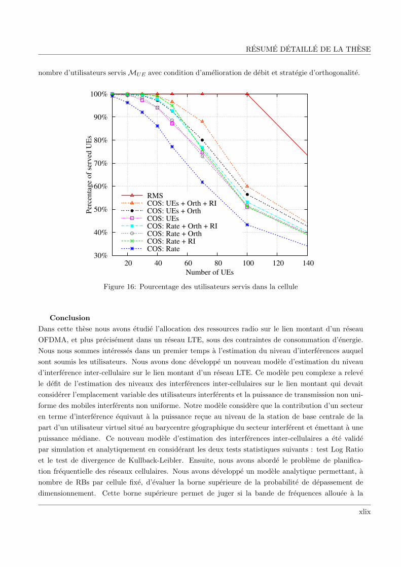
RESUME DETAILLE DE LA THESE
nombre d’utilisateurs servisMUE avec condition d’amelioration de debit et strategie d’orthogonalite.
30%
40%
50%
60%
70%
80%
90%
100%
20 40 60 80 100 120 140
Per
cen
tag
e o
f se
rved
UE
s
Number of UEs
RMSCOS: UEs + Orth + RICOS: UEs + OrthCOS: UEs COS: Rate + Orth + RICOS: Rate + OrthCOS: Rate + RICOS: Rate
Figure 16: Pourcentage des utilisateurs servis dans la cellule
Conclusion
Dans cette these nous avons etudie l’allocation des ressources radio sur le lien montant d’un reseau
OFDMA, et plus precisement dans un reseau LTE, sous des contraintes de consommation d’energie.
Nous nous sommes interesses dans un premier temps a l’estimation du niveau d’interferences auquel
sont soumis les utilisateurs. Nous avons donc developpe un nouveau modele d’estimation du niveau
d’interference inter-cellulaire sur le lien montant d’un reseau LTE. Ce modele peu complexe a releve
le defit de l’estimation des niveaux des interferences inter-cellulaires sur le lien montant qui devait
considerer l’emplacement variable des utilisateurs interferents et la puissance de transmission non uni-
forme des mobiles interferents non uniforme. Notre modele considere que la contribution d’un secteur
en terme d’interference equivaut a la puissance recue au niveau de la station de base centrale de la
part d’un utilisateur virtuel situe au barycentre geographique du secteur interferent et emettant a une
puissance mediane. Ce nouveau modele d’estimation des interferences inter-cellulaires a ete valide
par simulation et analytiquement en considerant les deux tests statistiques suivants : test Log Ratio
et le test de divergence de Kullback-Leibler. Ensuite, nous avons aborde le probleme de planifica-
tion frequentielle des reseaux cellulaires. Nous avons developpe un modele analytique permettant, a
nombre de RBs par cellule fixe, d’evaluer la borne superieure de la probabilite de depassement de
dimensionnement. Cette borne superieure permet de juger si la bande de frequences allouee a la
xlix

RESUME DETAILLE DE LA THESE
cellule est adequate ou non, tout en prenant en compte la charge du reseau, le comportement de
l’environnement radio, la QdS offerte aux utilisateurs et la politique d’allocation de ressources radio
utilisee. Le modele analytique de la borne superieure de la probabilite de depassement de dimension-
nement a ete developpe pour un systeme SISO et un systeme MIMO en considerant le gain de diversite
et le gain de multiplexage. En fonction de la probabilite de depassement de dimensionnement obtenue,
nous avons evalue la bande de frequences a allouer a une cellule et ajuste cette derniere en agregeant
une porteuse adequate afin de diminuer la probabilite de depassement de dimensionnement. Lorsque
la bande de frequences adequate est allouee a une cellule, nous avons propose un nouvel algorithme
base sur une politique opportuniste, qui alloue efficacement les RBs aux utilisateurs et permet de max-
imiser le debit total de la cellule. Les performances de cet algorithme ont ete etudiees dans un reseau
regulier et dans un reseau aleatoire, en les comparant aux algorithmes les plus references trouves dans
la litterature. Vu les resultats encourageants que nous avons obtenus, nous avons etendu l’application
de cet algorithme a un systeme multi-utilisateurs MIMO. Nous avons propose un nouveau decodeur
qui combine un decodeur zero forcing (ZF) et un maximum de vraisemblance (ML) pour annuler
l’interference entre les utilisateurs partageant le meme RB. Cette etude a ete faite pour differentes
metriques (metrique maximisant le debit par RB, et metrique maximisant le nombre d’utilisateurs par
RB) et un compromis a ete trouve en terme de maximisation de debit total de la cellule, en utilisant
la metrique de maximisation de nombre d’utilisateurs servis par RB, et en imposant des conditions
d’orthogonalite et d’amelioration de debit dans l’algorithme d’allocation de RBs aux utilisateurs.
l

Chapter 1
Introduction and Outline
1.1 Motivations
NOWADAYS, popularity of smart terminals, with their enhanced functionalities and ap-
plications, makes the Information and Communication Technologies (ICT) face more and
more serious challenges. The third Generation Partnership Project (3GPP) Long Term
Evolution (LTE) networks represent a major advance in cellular technology and their performances
accommodate the wireless broadband constantly increasing demand. LTE offers significant improve-
ments over previous technologies. Among them we can note that it provides a higher data throughput.
Actually, the system supports, within 20 MHz bandwidth, 75 Mbps in downlink and 50 Mbps in uplink
in Single Input Single Output (SISO) and up to 350 Mbps in downlink with 4×4 Multiple Input Mul-
tiple Output (MIMO) [15]. In addition, the simple system access architecture decreases the system
latency: only 10 ms of latency is needed to transmit data between users and the network [16].
Indeed, the Mobile Switching Controller (MSC) and Radio Access Controller (RNC), that are
placed respectively in the core network and the 2G and 3G Radio Access Network (RAN), do not
exist in LTE architecture. The LTE base station, commonly termed evolved NodeB (eNB), inherited
of some high level of RNC and MSC functionalities, such as mobility management and Radio Resource
Management (RRM). The remaining functionalities have been removed up to the Packet Core Network
(PCN) [17]. The RRM has a crucial role because a best use of radio resources can greatly improve the
system performances. The limited radio resources place the RRM as the main interest on researchers
to fully exploit LTE potentialities. The RRM is responsible of managing multi-user radio access and
determines the strategies and algorithms for allocating the radio resources to the users depending on
their individual Quality of Service (QoS) requirements and channel conditions.
1

CHAPTER 1. INTRODUCTION AND OUTLINE
In LTE, new multiple access techniques to the radio air interface, based on Orthogonal Frequency
Division Multiplex (OFDM) method, are introduced: Orthogonal Frequency Division Multiple Access
(OFDMA) in the downlink and Single Carrier Frequency Division Multiple Access (SC-FDMA) in
the uplink [18]. These access techniques allow a flexible bandwidth allocation (from 1.4 MHz to 20
MHz) [15], and an increase of the spectral efficiency (three or four times higher than the spectral
efficiency of High Speed Packet Access (HSPA) Release 6) [19]. In OFDMA, the available bandwidth
is divided into orthogonal subcarriers, whose narrowness is such that fading is considered as flat over
each of them. Consequently, their allocation to the users can be done according to the users channel
conditions over each subcarrier. Since the users are orthogonally multiplexed, the intra-cell inter-
ference is cancelled. The drawback of OFDMA is a high generated Peak to Average Power Ratio
(PAPR), which makes it irrelevant on uplink due to the User Equipment (UE) battery life. Unlike
OFDMA, SC-FDMA generates a low PAPR, by considering the whole allocated subcarriers as a single
carrier and sharing equally the UE transmission power over it [20] [21] [22]. The LTE release 8 stan-
dards impose on each UE to be allocated contiguous subcarriers and to use the same Modulation and
Coding Scheme (MCS) over its whole allocated subcarriers [23]. Due to these two SC-FDMA specific
constraints, the RRM algorithms proposed for the downlink can not be directly applied to the uplink.
Radio resource allocation process occurs each Transmission Time Interval (TTI) of 1 ms duration,
it is performed throughout the allocation of Resource Blocks (RB), which are the smallest grid that
can be allocated to one UE. Each user can be allocated more than one RB to guarantee its required
QoS. The LTE standardized bandwidth contains a fixed number of RBs [3]. To benefit from the
full performances of the system, we should efficiently allocate the limited number of RBs in order
to increase the cell’s capacity, to serve more users and to prevent from wasting radio resources. In
addition, radio resource allocation should be processed with low computational complexity, as it occurs
recursively every 1 ms and potentially concerns a large number of heterogenous users in highly loaded
networks.
1.2 Contributions
The main purpose of this dissertation is to show how we can efficiently allocate the flexible bandwidth
to each cell (or sector) regarding the QoS required by the users and minimizing their dimensioning out-
age probability due to insufficient resources. Once the frequency planning is performed, the allocation
of radio resources in uplink LTE networks is discussed. We consider a distributed resource allocation
architecture, where each eNB allocates radio resources independently of the radio resources allocation
decision of the other eNBs of the network. In this context, radio resources allocation includes both the
allocation of RBs to the users and the determination of the UEs transmission power. In addition, the
RB allocation entity respects the SC-FDMA technique constraints and aims at maximizing the system
satisfaction level. It is then extended to the Multi-User MIMO (MU-MIMO) case, where one RB can
be shared by several users. Green power allocation is also studied, where the UE transmission power is
2

1.2. CONTRIBUTIONS
established according to the user’s QoS requirements and the radio channel conditions experienced by
the concerned user over its whole allocated RBs. UE transmission power reduction leads to decrease
the Inter-Cell Interference (ICI). Consequently, a new model of ICI estimation is proposed for the
uplink, adapted to the Power Control (PC) applied on the UE transmission powers.
The main objectives of the studies performed in this thesis are:
• to estimate the inter-cell interference in uplink green LTE networks. Since ICI is caused by the
use of the same resources by other users in the neighboring cells, then the ICI level, in uplink,
depends of the transmission power of these interfering users. However, in case of UE power
control application, the ICI level is different from the one used while the UE transmission powers
are set at their maximum. For that purpose, we propose a low computational complexity model
of ICI level estimation received at the eNB over each RB when UE power control is applied.
• to propose an analytical model for the dimensioning outage probability evaluation, which helps
the radio dimensioning of uplink LTE networks. To allocate an adequate bandwidth to each cell
(or sector) according to the network’s load and the user’s QoS, an analytical model of the di-
mensioning outage probability is developed. This model evaluates analytically the upper bound
of the probability that users are in outage because of insufficient resources. The upper bound
of the dimensioning outage probability, by considering the network’s configuration, helps us to
determine the required number of RBs that should be allocated to the cell (or sector), with the
corresponding maximum dimensioning outage probability. An average number of RBs needed
to serve the users, by considering the RB allocation policy and the users QoS requirements,
is computed. The fair RB allocation algorithm and the opportunistic RB allocation algorithm
are investigated. The dimensioning outage probability upper bound is evaluated for one and
multiple users QoS classes. This study is also extended to the MIMO systems.
• to determine a low computational complexity radio resource allocation scheme, which aims at
maximizing the aggregate throughput of the network with a low UE transmission power. Our aim
is an efficient allocation of the radio resources to users, with respect to the release 8 SC-FDMA
constraints. The RBs are efficiently allocated to the users according to their individual channel
conditions and QoS requirements. Then, an adjustment of UE transmission power is performed
without affecting the throughput achieved by the concerned user before the transmission power
reduction. The performances of the proposed radio resource allocation scheme are given in
regular and random networks. The RB allocation algorithm performance analysis is extended
to the MU-MIMO systems, where the spectrum efficiency is improved. An adaptation of the
RB allocation algorithm for the LTE-Advanced (LTE-A) networks is also investigated.
3

CHAPTER 1. INTRODUCTION AND OUTLINE
1.3 Assumptions
Throughout this thesis, we make some assumptions that are given in the following:
• Distributed radio resource allocation architecture:
Each eNB is responsible of the radio resource allocation over its served users, without considering
the resource allocation decision made by the neighboring eNBs. The radio resource allocation
is based on the radio channel conditions given by the Channel State Information (CSI).
• Network topology :
Except Chapter 4, tri-sectored antennas are used. To manage ICI, we allocate different frequency
bandwidths at each sector and adopt a 1 × 3 × 3 frequency reuse pattern. Two topologies are
used: a regular topology and a random topology. The regular one is a grid of hexagonal cells
where users are classified into each sector regarding to their geographical positions. The random
topology is a superposition of Poisson point processes of intensity λeNB and λUE that represent
respectively the eNBs and the UEs. The sector selection, in random networks, is given with
respect to the Reference Signal Received Power (RSRP), where a comparison of the downlink
received power from each sector is performed.
• Knowledge of the channel conditions:
We assume a full knowledge of the channel conditions at the receiver. This knowledge is due to
the CSI that estimates the propagation of the signal including the shadowing and fading effects
with help of the Reference Signals (RS). These RS are sent both in uplink and downlink in a
specific resource element (RE) of each RB.
• Frequency Division Duplexing (FDD) mode:
We consider a LTE FDD mode, where the uplink and the downlink transmissions operate in
two different bandwidths. The FDD LTE frame structure of 10 ms duration is considered. Each
frame is divided into ten subframes and each subframe consists of two time slots.
• Resource allocation:
The resource allocation process occurs each TTI which corresponds at one subframe of 1 ms
duration. As the allocated resources are of 0.5 ms duration, the allocated resources in the first
slot of one subframe are maintained for the second slot. Since the resource allocation is based
on the channel state information on each resource, then the metric used to allocate the radio
resources is averaged over the two slots. We consider a perfect synchronization between UEs
and eNB, with the standardized Cyclic Prefix (CP). Thus, the Inter-Symbol Interference (ISI)
is assumed to be null.
4

1.4. THESIS OUTLINE
• Users Traffic:
The users are drawn uniformly in the area. We assume that each active user has an infinite
backlog of data to send. Our objective is to maximize the aggregate throughput of the network;
therefore we allocate to the users the radio resources that maximize their individual throughput,
except in Chapter 4, where the upper bound of the dimensioning outage probability is established
considering a target throughput of each user, and in Chapter 5, when QoS differentiation RB
allocation algorithm is proposed.
1.4 Thesis outline
The optimization of radio resource allocation is investigated. In Chapter 2 the technical and math-
ematical necessary background is given. Since it is based on the channel state information of each
UE on each radio resource, the ICI level is first estimated in green LTE network (Chapter 3). Then,
we aim at determining the adequate allocated bandwidth to each cell (or sector) according to a given
maximum dimensioning outage probability. The analytical model of the dimensioning outage prob-
ability upper bound is developed, for SISO and MIMO systems, in Chapter 4. Once the allocated
bandwidth is performed, the algorithms and strategies for radio resource allocation are studied in
Chapter 5. They include the allocation of resource blocks and the UE transmission power. Then, the
RB allocation study is expanded to MU-MIMO system in Chapter 6.
• Chapter 2 - Preliminaries
Chapter 2 provides the technical and mathematical background needed in this thesis. The tech-
nical background concerns the LTE system technical specificities: radio resource management,
modulation and coding scheme, QoS, MIMO and MU-MIMO techniques, and the main simula-
tion parameter considered in this thesis. The mathematical background consists of the Poisson
point process and the marked Poisson point process which are used in Chapter 4 to evaluate
the dimensioning outage probability upper bound.
• Chapter 3 - Inter-cell interference estimation in green LTE networks
This chapter investigates the inter-cell interference estimation in the uplink of green LTE net-
works. We propose a new model of inter-cell interference estimation when the UE transmission
power control is applied. The proposed model is given in a regular network where the location
and the controlled power of each user is assumed known. This model has low computational
complexity and it avoids Monte Carlo simulations. The ICI estimation model is validated both
analytically and by simulations.
• Chapter 4 - dimensioning Outage probability upper bound depending on RRM
Chapter 4 focuses on dimensioning uplink LTE networks. We propose an analytical model
to evaluate an upper bound of the probability that users are blocked because of an insufficient
number of resources. This upper bound helps cell planners to estimate the network configuration
and the necessary allocated bandwidth to each cell. The number of RBs allocated to each UE is
established as a function of its required QoS. The study is expanded to the multiple QoS class
5

CHAPTER 1. INTRODUCTION AND OUTLINE
in SISO system. The diversity and multiplexing gains in MIMO systems are also investigated.
• Chapter 5 - Radio resource allocation scheme for green LTE networks
In this chapter, we focus on the uplink radio resource allocation. It includes algorithms and
strategies to allocate RBs to the UEs and to adjust their transmission power. Two algorithms
are proposed: the Opportunistic and Efficient RB Allocation (OEA) algorithm and the Quality
of Service based Opportunistic and Efficient RB Allocation (QoS based OEA) algorithm. These
algorithms allocate efficiently the RBs, while respecting the LTE release 8 SC-FDMA constraints.
An adaptation of these two algorithms for LTE-A networks is investigated. The UE power
allocation consists of allocating the lowest possible power to each UE without affecting its
individual throughput. The simulation performances are given in regular and random networks,
which allow us to analyze the RB allocation algorithms stability.
• Chapter 6 - Radio resource management in MU-MIMO
In this chapter, the proposed OEA algorithm discussed in Chapter 5 is extended to MU-MIMO
networks. For this, we first propose a new transceiver structure that gives the possibility to spa-
tially multiplex different UEs data streams and offers to each UE a reliable individual throughput
by exploiting the transmit and receive diversity. Then, we show, using this transceiver structure,
how to extend the OEA algorithm in the MU-MIMO context.
6

1.5. LIST OF PUBLICATIONS
1.5 List of publications
International journals
• F.Z. Kaddour, E. Vivier, L. Mroueh, M. Pischella and P. Martins, “Green Opportunistic and
Efficient Resource Block Allocation Algorithm for LTE Uplink Networks”, submitted to IEEE
Transaction on Vehicular Technology.
International conferences
• F.Z. Kaddour, E. Vivier, M. Pischella, L. Mroueh and P. Martins, “Green Opportunistic and
Efficient Resource Block Allocation Algorithm for LTE Uplink Networks ”, in proceedings of
3rd IEEE GreenComm online conference, Oct. 2013.
• M.V.V. Reddy, E. Vivier, F. Z. Kaddour, “Joint benefits of Fractional Frequency Reuse and
Relays in LTE Networks ”, in proceedings of 3rd IEEE GreenComm online conference, Oct.
2013.
• L. Mroueh, E. Vivier, F.Z. Kaddour, M. Pischella and P. Martins, “Combined ZF and ML
Decoder for Uplink Scheduling in Multi-User MIMO LTE Networks ”, in proceedings to IEEE
International Symposium on Personal, Indoor and Mobile Radio Communications (PIMRC),
London, UK, Sept. 2013.
• F.Z. Kaddour, P. Martins, L. Decreusefond, E. Vivier and L. Mroueh, “Outage probability
upper’s bound in uplink Long Term Evolution networks with multi QoS users classes ”, in
proceedings of IEEE Global Communications conference (GLOBECOM), Atlanta, USA, Dec.
2013.
• F.Z. Kaddour, M. Pischella, P. Martins, E. Vivier and L. Mroueh, “Opportunistic and Effi-
cient Resource Block Allocation Algorithms for LTE Uplink Networks”, in proceedings of IEEE
Wireless Communications and Networking Conference (WCNC), Shanghai, China, Apr. 2013.
• F.Z. Kaddour, E. Vivier, M. Pischella and P. Martins, “A New Method for Inter-Cell Interfer-
ence Estimation in Uplink SC-FDMA Networks”, in proceedings of IEEE Vehicular Technology
Conference (VTC) Spring 2012, Yokohama, Japan, May. 2012.
• A. Kessab, F.Z. Kaddour, E. Vivier, L. Mroueh, M. Pischella and P. Martins, “Gain of Multi-
Resource Block Allocation and Tuning in the Uplink of LTE Networks”, in proceedings of IEEE
International Symposium of Wireless Communication System (ISWCS), Aug. 2012.
7

CHAPTER 1. INTRODUCTION AND OUTLINE
8

Chapter 2
Preliminaries
AS A STARTING point of this thesis, this chapter provides a background on the technical
and the mathematical tools that will be relevant to further developments. Some technical
preliminaries on various aspects of LTE systems are introduced with a special focus on the
uplink of radio resource management. Both physical and Medium Access Control (MAC) layers are
also detailed. Then, we provide a unified system model for wireless transmission taking into account
Single Input Single Output (SISO), Multiple Input Multiple Output (MIMO) and Multi-User MIMO
(MU-MIMO) systems. Finally, we provide some mathematical background on the Poisson point
process. These tools will be later used in Chapter 4 to compute the dimensioning outage probability
due to the lack of resources in LTE networks.
2.1 LTE system technical specificities
In this section, we review from [24] [9] the main specificities of the LTE system covering its performance
targets and the physical and medium access layers. We also provide a comparative study of the
advantage in terms of PAPR1 of the use of SC-FDMA technique rather than OFDMA one.
2.1.1 LTE performance targets
The goal of LTE standards aim at creating a new technology providing higher data rates, larger
coverage area, lower latency and higher spectral efficiency. These objectives are largely reached due to
a new architecture and a new air interface. LTE is a simplified architecture which refers to a reduced
number of access nodes between the UEs and the core network. Only the eNB is considered as an
1PAPR is a ratio between the peak amplitude squared and the average power squared.
9

CHAPTER 2. PRELIMINARIES
access component in the Evolved-Universal Terrestrial Radio Access Network (E-UTRAN), between
UE and the Evolved Packet Core (EPC) network. It is considered as the terminal point of the RAN.
LTE realize on OFDMA modulation. It supports a flexible bandwidth which can be 1.4, 3, 5, 10,
15 and 20 MHz [9]. It is useful for mobile operators that can not guarantee a contiguous 20 MHz
bandwidth on account of the fragmentation of spectrum allocation. The flexible bandwidth allows
several combinations of Carrier Aggregation (CA), that are added in LTE-A (Release 10). Actually,
each component carrier has one of the standard bandwidths cited above, and the maximum number of
carrier components that can be aggregated, is set to five. Thereby, the maximum allocated bandwidth
reaches 100 MHz [25]. Within a 20 MHz bandwidth, the LTE peak data rate reaches 75 Mbps in
downlink and 50 Mbps for SISO uplink, and up to 350 Mbps in uplink with 4 × 4 MIMO antennas.
In the SISO case, the peak data rate corresponds to 5 bps/Hz in downlink and 2.5 bps/Hz in uplink,
which is higher than the spectral efficiency reached with the HSPA networks [19].
2.1.2 Orthogonal Frequency Division Multiplexing
The wireless local area networks IEEE 802.11a and wireless metropolitan area networks IEEE 802.16-
2004 standards are the first technologies which introduce the multi-carrier technique by using OFDM/TDMA
mode, in the communication networks. OFDMA was first adopted in 2005 by the mobile services of
WiMAX [26]. But it was revealed by the 3GPP LTE which adopted it in downlink and adapted it for
the uplink by introducing the SC-FDMA. OFDM divides the available bandwidth into orthogonal nar-
rowband subcarriers. This results in a flat fading channel in each subcarrier. The subcarriers can then
be allocated in an opportunistic way. Each UE will be allocated subcarriers where it experiences good
radio channel conditions. The techniques based on OFDM modulation are efficient in opportunistic
allocation. Increasing the number of subcarriers introduces a multi-user diversity. Consequently, the
probability that all the users are in a deep fade in all subcarriers decreases. The data symbols are
transmitted over orthogonal subcarriers which leads to an inter-symbol interference cancellation. The
orthogonality is obtained with an Inverse Fast Fourier Transform (IFFT) at transmission, and a Fast
Fourier Transform (FFT) at reception with an adequate regular spacing frequency [21]. The robustness
of the OFDM technique in case of multi-path is reached with the insertion of the Cyclic Prefix (CP).
The CP is a duplication of the last temporal information of each OFDM symbol at the beginning of
this symbol (Figure 2.1). Then, even in case of delay in radio transmission, all the symbols will be
recovered.
NFFT+CP
CP NFFT
Figure 2.1: Cyclic Prefix of an OFDM symbol
10

2.1. LTE SYSTEM TECHNICAL SPECIFICITIES
2.1.3 OFDM based LTE multiple access techniques
In the following, two access technique based on OFDM are presented: the OFDMA and the SC-FDMA.
Orthogonal Frequency Division Multiple Access - OFDMA
OFDMA is a multiple access technique based on OFDM physical layer. It allows a multiple access
and shares simultaneously the available frequency bandwidth over multiple users. The drawback of
the OFDMA technique is the high generated PAPR, which relates on the power amplifier efficiency
at the transmitter. The power amplifier should operate in very large linear region to overcome the
distortion of the signal peaks into non-linear region. This leads to an increase of the power amplifier
complexity design and an expensive UEs.
Single Carrier Frequency Division Multiple Access - SC-FDMA
Due to a high PAPR, OFDMA use in uplink is not adapted to mobile terminal constraint (because of
the battery autonomy). Then, its variant SC-FDMA, termed also DFTS-OFDM (for Discrete Fourier
Transform Spread-OFDM), was adopted for the uplink of the LTE networks. This technique consists
in adding a FFT at the beginning of the transmission (before the subcarrier mapping) and an IFFT at
the end of the reception (after the subcarrier remapping and equalization). With FFT/ IFFT a large
number of zeros symbols are added to obtain a power 2 number of subcarriers. This aims at reducing
the PAPR [21]. Both OFDMA and SC-FDMA techniques block diagrams are given in Figure 2.2.
Demod-
dulationFFT
S to P Remove
CP
Analog
to
DigitalP to S
S to P Modu-
lationIFFT
P to S Add
CP
Digital
to
Analog
+SC-FDMA
OFDMA
FFT
IFFT
Figure 2.2: OFDMA and SC-FDMA technique block diagrams for LTE
SC-FDMA advantages
Thanks to the FFT mapper block added by the SC-FDMA technique, which spreads the informa-
tion over multiple subcarriers, the SC-FDMA inherits of the OFDM frequency diversity gain. Two
11

CHAPTER 2. PRELIMINARIES
SC-FDMA types were proposed: Interleaved SC-FDMA (I-SC-FDMA) and Localized SC-FDMA (L-
SC-FDMA). In I-SC-FDMA, the symbols are spread over subcarriers and complete the N points of
FFT with zeros symbols in-between. L-SC-FDMA centralizes the data symbols in a portion of adja-
cent subcarriers and complete the N FFT points with zero symbols as shown in figure 2.3.
Since the information are spread over the entire bandwidth, the I-SC-FDMA is more robust to the
from FFT to FFT
00
0
0
0
0
0
from FFT to FFT
L-SC-FDMA I-SC-FDMA
Figure 2.3: Interleaved and Localized SC-FDMA
frequency selective fading and offers an additional frequency diversity gain compared to the classical
OFDMA. The L-SC-FDMA, in combination with a channel dependent scheduling, can potentially
offer multi-user diversity in frequency channel conditions [20].
The major advantage of SC-FDMA over OFDMA is the low generated PAPR while transmitting the
signal. Authors of [22] compare the generated PAPR between OFDMA and the two SC-FDMA types:
I-SC-FDMA and L-SC-FDMA. The study reveals that the I-SC-FDMA gives better performances
than the L-SC-FDMA. Actually, I-SC-FDMA generates a PAPR, in case of QPSK modulation, which
is about 10 dB lower than the one generated by OFDMA. Whereas, the PAPR generated by the
L-SC-FDMA is only about 3 dB lower. However, the SC-FDMA modulated signal can be viewed
as a single carrier signal. A pulse shaping filter can be applied to the transmitted signal. As a re-
sult, the PAPR performances of I-SC-FDMA are degraded, while the L-SC-FDMA performances are
unchanged [20] [22]. Consequently, the overall PAPR performances of L-SC-FDMA are better than
the I-SC-FDMA ones. Therefore, L-SC-FDMA was finally adopted for the uplink of LTE release 8
networks.
As a consequence for our thesis, the subcarriers adjacency constraint will be considered for radio re-
source allocation to UEs. This constraint will not be taken into account in LTE-A networks. Actually,
since carrier aggregation was adopted by the standards in LTE-A in order to increase the data rate,
the component carriers can belong to different operating bandwidth. Then, in order to support the
carrier aggregation in the uplink, as well in downlink, the I-SC-FDMA was adopted which enables
frequency selective scheduling within carrier components [27].
12

2.1. LTE SYSTEM TECHNICAL SPECIFICITIES
2.1.4 LTE RB allocation constraints
By adopting L-SC-FDMA in LTE release 8, the RB allocation in our thesis should consider the
following constraints:
1. Contiguity constraint: the L-SC-FDMA technique requires contiguous subcarriers for each
UE. Then to obtain an optimal PAPR, the RBs allocated to each UE should also be contiguous
in the frequency domain.
2. Modulation and Coding Scheme (MCS) robustness: the MCS summarizes the modula-
tion type and the coding rate that are possible for data transmission. The MCS configuration
depends on the radio channel conditions, expressed by the Signal to Interference plus Noise
Ratio (SINR) experienced by each UE on each RB. The SINR level translates the received sig-
nal and the receiver ability to decode correctly the sent information. The SINR level required
for each modulation and coding scheme is given in Table 2.1, taken from [2] and restricted
to the MCS considered in this thesis: QPSK, 16 QAM and 64 QAM modulations with 12 ,
23
and 34 coding rates. The high order modulation is more sensitive to bad channel conditions
than the low order modulations, due to higher density constellation that the receiver should
decode. Thereby, the adapted coding rate should be chosen in order to allow error correction.
To keep the control information overhead small, the same MCS is used by each UE over its
whole allocated bandwidth [28]. This constraint is called the MCS robustness.
SINR range (dB) Modulation Code rate
−7 < SINR ≤ −5 QPSK 0.07
−5 < SINR ≤ −3 QPSK 0.11
−3 < SINR ≤ −1 QPSK 0.18
−1 < SINR ≤ 1 QPSK 0.30
1 < SINR ≤ 3 QPSK 0.43
3 < SINR ≤ 5 QPSK 0.58
5 < SINR ≤ 7 16QAM 0.36
7 < SINR ≤ 8.5 16QAM 0.47
8.5 < SINR ≤ 10 16QAM 0.60
10 < SINR ≤ 11.5 64QAM 0.45
11.5 < SINR ≤ 13.5 64QAM 0.55
13.5 < SINR ≤ 15 64QAM 0.65
15 < SINR ≤ 17 64QAM 0.75
17 < SINR ≤ 19.5 64QAM 0.85
SINR ≥ 19.5 64QAM 0.92
Table 2.1: SINR to Code rate mapping [2]
The contiguity constraint makes the RB allocation less flexible and adds more challenges to the
RRM entity. Thus, most RRM strategies proposed for LTE downlink can not be directly used for
the uplink. For this purpose, new RB allocation algorithms, respecting the LTE release 8 SC-FDMA
constraints, are proposed in Chapter 5. Since the I-SC-FDMA technique is used for LTE-A networks,
13

CHAPTER 2. PRELIMINARIES
the contiguity constraint is cancelled, while maintaining the MCS robustness constraint. Thus, we
prove that with small modifications, our proposed RB allocation algorithms, can also be applied to
LTE-A networks.
2.1.5 Uplink LTE frame structure
Considering LTE FDD, the same frame structure is applied in both uplink and downlink. Each frame
consists of ten subframes of 1 ms each. One subframe is defined as two consecutive slots, where the
time slot duration is 0.5 ms. In case of SC-FDMA technique, the signal transmitted in each slot is
described with a grid of NULRB contiguous RBs. One RB is the smallest grid that can be allocated to
one UE. It consists of NRBsc equal to 12 consecutive subcarriers and NUL
symb equal to 6 or 7 SC-FDMA
symbols according to the prefix cyclic type [24]. The frame structure described in Figure 2.4 considers
a normal cyclic prefix.
Different number of RBs are available according to the flexible standardized LTE bandwidths, as
detailed in Table 2.2.
Channel bandwidth (MHz) B 1.4 3 5 10 15 20
FFT size 128 256 512 1024 1536 2048
Number of subcarriers 72 180 300 600 900 1200
Number of available RBs 6 15 25 50 75 100
Table 2.2: Bandwidth vs number of available RBs [3]
2.1.6 QoS in LTE
Unlike previous cellular systems, LTE has been designed to support only packet-switched services.
It aims at providing seamless IP connectivity between UEs and the Packet Data Network (PDN),
without disturbing the user’s applications during mobility. QoS support in LTE is provided through
an Evolved Packet System (EPS) bearer. An EPS bearer is established when a UE connects to the
PDN and is categorized into either a Guaranteed Bit Rate (GBR), or a non Guaranteed Bit rate
(non-GBR) bearer, depending on whether the user has a minimum guaranteed bit rate requirement
or not. The QoS parameters that are set and controlled by a Policy and Charging Control (PCC)
architecture within the EPC network are: the Allocation Retention Priority (ARP) which helps the
network to decide which RBs are kept in congestion case, the Maximum Bit Rate (i.e. a limit on data
rates: no radio bearer exhausts the network resources), the GBR, and the QoS Class Identifier (QCI).
The QCI defines a set of characteristics that describe the packet forwarding treatment between the
UE and the EPC. These characteristic are: the bearer type, the packet delay budget (between the UE
and the EPC), and the Packet Loss Rate. They are summarized in the 3GPP standards [29].
14

2.1. LTE SYSTEM TECHNICAL SPECIFICITIES
0 1 2 3 10 11 19
One frame (10 ms)
One subframe (1 ms)
One slot (0.5 ms)
Sub
carr
iers
Symbols
Resource element (m,n)
Resource block
SC-FDMA symbols
n
m
NRBsc ×NUL
symb resource elements
Figure 2.4: LTE FDD frame structure
2.1.7 Radio resource management
The parameters cited above are considered by the Radio Resource Management (RRM) which plays
a crucial role in LTE networks by managing the limited radio resources in such a way that the radio
transmission is as efficient as possible. In E-UTRAN, the role of RRM focuses on two major tasks:
1. Radio Admission Controller (RAC): which is responsible for examining UEs admission
requests for new connections. The admission control is performed considering the available
resources, the current network’s load and the QoS required by the UEs [28].
2. Packet Scheduler (PS): which refers to the allocation of RBs to the UEs considering the link
adaptation. According to [30], the PS can be uncoupled into two entities : (i) Time Domain
Packet Scheduling (TDPS) which establishes the priority between the users selected by the
RAC, and (ii) Frequency Domain Packet Scheduling (FDPS) which searches the pair (RB,UE)
that maximizes the utility function. These two entities are illustrated on Figure 2.5.
Adapted management of radio resources optimizes the system performance and also reduces the cost
per bit transmitted over the radio interface. In SISO, the number of users that can be served during
one TTI is limited by the number of available RBs in the allocated bandwidth (the number of served
15

CHAPTER 2. PRELIMINARIES
Time Domain
Packet Scheduling
Frequency Domain
Packet Scheduling
QoS requirements
CSI
Active UE
Figure 2.5: Packet Scheduler design
users will not exceed the number of available RBs within the allocated bandwidth Table 2.2). The
uplink scheduler must map efficiently the RBs among users considering the limited UE transmission
power. LTE uplink scheduling can be addressed as an optimization problem, where the desired solution
is the mapping between the schedulable UEs and the RBs, that maximizes the desired performance
target. Solving the scheduling problem can be very complex due to the high number of factors to take
into account, as well as the virtually unlimited number of scheduling patterns to examine. In addition,
the packet scheduler faces the hard-time constraints where the scheduling is done at the frequency of
subframes which corresponds to one TTI. As the TTI duration is equal to 1 ms, the scheduler has
only few milliseconds to come up with the optimal allocation scheme. We can divide the scheduling
problem in two subproblems :
1. Utility function: a mathematical function that translates into a metric the satisfaction of
the system related to its target. These target requirements can refer to performance metrics
such as data throughput (total throughput of the system or throughput per UE), fairness (in
terms of throughput or resources), minimization of transmission power, or minimization of the
dimensioning outage probability. The utility function depends on the metrics used in the time
domain (MTD) and the frequency domain (MFD) packet scheduling respectively. The utility
function that user k experiences in the resource block c can be computed as :
Uk →MTD(k).MFD(k, c) (2.1)
Usually, MTD and MFD measure the quality of the radio channel. In this case, the scheduler
is called channel-dependent.
2. Allocation policy: the allocation policy involves the strategies and algorithms that the net-
work adopts to allocate the radio resources to the users. These strategies are defined by the
operators. Dynamic resource allocations are applied. They take the users QoS requirements
into consideration in order to satisfy the served users. The allocation policy aims at limiting
the network’s congestion and enhancing the service quality [31].
16

2.2. WIRELESS CHANNEL MODEL
In this thesis, only the frequency domain packet scheduling is considered. Since the metric used is
the SINR experienced by each UE over each RB at each TTI, and the allocations of RBs performed
at each TTI are independents, we prefer to use for the algorithm we propose the term RB allocation
instead of scheduling.
Chapter 4 focuses on fair and opportunistic RB allocation algorithms to evaluate the dimensioning
outage probability upper bound. These two algorithms are the extreme cases. The dimensioning
outage probability of other RB allocation algorithms will be lower bounded and upper bounded by
opportunistic and fair RB allocations. In Chapter 5, other RB allocation algorithms are investigated,
such as the OEA and the QoS based OEA algorithms. The proposed algorithms are compared with
the most cited RB allocation algorithms for LTE uplink networks, in the literature. An extension of
the algorithm is proposed in MU-MIMO context (Chapter 6).
2.2 Wireless channel model
In this section, we provide a unified model for the propagation over the wireless channel when com-
municating over the uplink channel, from the UE towards the eNB. We first review the modeling of
the transmission of SISO system when using OFDM technique and, taking into account the eNB and
UE transmission power’s and antenna’s gains, the path loss propagation model, the fading and the
shadowing parameters. Then, we define for this channel model the effective SINR computation. We
give then a brief overview on the MIMO systems and the diversity and spatial division multiplexing
techniques. Then, we show how to compute the MIMO effective SINR using optimal and sub-optimal
decoders. Finally, we recall the system model of multi-user MIMO uplink systems, focusing on the
capacity region and the Spatial Division Multiple Access (SDMA) techniques.
2.2.1 Cell types
There are four types of cells in LTE networks: macrocells, microcells, picocells, and femtocells. For
urban areas, the cells used are macrocells, which cover areas in kilometers and serve a hundreds of
users. Microcells cover smaller areas, and are added to improve the coverage in dense urban areas. In
this thesis, we consider only macrocells, where the maximum inter-site distance in the regular network
is set to 1.7 km. We assume that the eNBs are installed at a 30 m height and radiate with a maximum
power PeNB equal to 20 W (equivalent to 43 dBm).
2.2.2 User Equipment class
The user equipment is the device used directly by the end user to communicate. It can be a hand-
held telephone, a laptop computer equipped with a mobile broadband adapter, or any other device.
Whatever the device, the UE specifications are given by the LTE standards. In [32], four UE classes
are defined. Each class of UE has its specific transmission power and its tolerance. In this thesis, a UE
17

CHAPTER 2. PRELIMINARIES
class 3 is used, implying a maximum transmission power Pmax equal to 125 mW which is equivalent
to 21 dBm.
2.2.3 Propagation model
Unlike wired media, the wireless medium is unreliable due to its broadcast nature and the propagation
environment effects. The transmitted signal from the UE to the eNB which are separated with
a distance r undergoes an attenuation due to the radio waves propagation, called path loss. To
predict the signal attenuation and the coverage by the same way, many statistical models are proposed
according the used frequency band, the type of deployment (urban, suburban, rural, etc), and the type
of used technology. The most widely used propagation models are summarized in [33]. In LTE, there
are three models that can be used: Okumura Hata, COoperation in Science and Technology (COST-
231) and International Mobile Telecommunication (IMT-2000). In this dissertation, the Okumura
Hata propagation model for urban area is used [5], where the path loss is expressed as:
PL(r) = Kr−β (2.2)
with, K the path loss constant equal to 10−a10 , and β is the path loss exponent equal to b
10 . The
parameters a and b are computed according to the frequency carrier fc and the UE and eNB heights
set respectively to 1.5 m and 30 m. Table 2.3 summarizes the obtained Okumura Hata propagation
model parameters according to the used frequency carrier.
fc(MHz) a b
2600 137.7 34.4
800 117.85 34.4
Table 2.3: Okumura Hata propagation model parameters
2.2.4 eNB and UE antennas gains
Gains of antennas used for transmission and reception aim at improving the signal strength. Except in
Chapter 4 where the eNB antenna is considered as omnidirectional with 0 dBi gain, in the rest of the
thesis, tri-sectored eNB antennas are considered, whatever the network topology: regular networks
or random networks. The antenna’s radiation pattern used at each sector, taken from the LTE radio
frequency system scenarii given in the standards [34], is expressed in dB as:
(GA(θ))dB = (GeNB)dB −min
12
(θ
θ3dB
)2
, Am
, −180 ≤ θ ≤ 180 (2.3)
where GeNB is the eNB antenna gain set to 17 dBi in the boresight direction, θ3dB is the 3 dB beam
width equal to 70, and Am is the maximum attenuation set to 20 dB.
In regular networks equipped with tri-sectored antennas, the angle between the users of each sector
18
2.2. WIRELESS CHANNEL MODEL
and the antenna boresight does not exceed 60. In this case, the antenna radiation pattern can be
written as:
(GA(θ))dB = (GeNB)dB − 12
(θ
θ3dB
)2
, −60 ≤ θ ≤ 60 (2.4)
This simplified antenna radiation pattern will be used in Chapter 3 for the ICI estimation analytical
model.
The UE is equipped with an omnidirectional antenna with a transmission gain GM = 0 dBi [32]. To
be able to use the MIMO technique in Chapter 4 and 6, the UE will have four omnidirectional antennas.
2.2.5 Shadowing and fading effects
In addition to the path loss, the radio waves can encountered some obstacles that are present on the
path. Then, the transmitted signal can be scattered, reflected or diffracted, which leads to additional
attenuations. Each path can have a different amount of attenuation and delay. Two major effects are
considered in this thesis:
a)- Shadowing
Shadowing is considered as a large-scale fading which results of attenuations due to signal
diffraction around large objects in the propagation path. In our dissertation, we note the
shadowing attenuation parameter As, which is modeled with a log-normal distribution.
b)- Fast fading
Fast fading coefficients, noted h, refer to rapid variations of the signal levels, due to multi-path
scattering effects, time dispersion, and Doppler shifts that arise from relative motion between
the transmitter and the receiver. Fast fading is called Rayleigh fading or Rician fading because
when a large number of reflective paths is encountered, the received signal envelope is described
by a Rayleigh or Rician probability density function (PDF)2. Considering, in this thesis, an
urban area with multiple reflective paths with No-dominant Line-Of-Sight (NLOS) propagation
path, Rayleigh fading is used.
1. Uncorrelated Rayleigh fading
Assuming uncorrelated fast fading, we consider the fading coefficients h as random vari-
ables following a Rayleigh distribution : h ∼ Rayleigh(σ), if h =√X2 + Y 2, where the
variables X and Y , following a normal distribution, i.e. X ∼ N(0, σ2) and Y ∼ N(0, σ2),
are considered as independent. The uncorrelated fading coefficients are used for: 1) the
robustness analysis of the ICI estimation model over fading effects (Chapter 3), and 2)
the dimensioning study in MIMO systems (Chapter 4).
2. Frequency correlated Rayleigh fading
In the case of frequency correlated Rayleigh fading, the fading coefficients hm with 1 ≤m ≤ NRB
sc , are considered to be correlated in the frequency domain. So, each user expe-
2The Rice distribution is a generalization of the Rayleigh distribution.
19

CHAPTER 2. PRELIMINARIES
riences a correlated fading over the subcarriers, with respect to the coherence bandwidth
Bc. To generate a frequency correlated Rayleigh fading, a Fourier Transform of the Power
Delay Profile (PDP) is used [1] [35]. Pedestrian users are considered in our simulation.
The corresponding PDP value for six paths, taken from [4], are given in Table 2.4. The
resulting frequency correlated fading coefficients are illustrated in Figure 2.6 for a band-
width of 10 MHz and an FFT size of 1024. The frequency correlated Rayleigh fading is
0 200 400 600 800 1000 12000
5
10
15
20
25
30
35
40Rayleigh fading
h2
subcarreir
Figure 2.6: Correlated Rayleigh Fading-FFT based approach
used in instantaneous simulations such as in our thesis, for the performance study over
one TTI of the RB allocation algorithm in MU-MIMO systems (Chapter 6).
Power of path (pk) [dB] 0 −1 −9 −10 −15 −20
Path delay (τk) [µs] 0 0.3 0.7 1.1 1.7 2.5
Table 2.4: Multi-tap channel: power delay profile [4]
3. Time-frequency correlated Rayleigh fading
Here, we consider that each UE experiences different fast fading coefficient h(m,n) over
the different resource elements of one RB (i.e. 1 ≤ m ≤ NRBsc and 1 ≤ n ≤ NUL
symb).
The fast fading coefficients are assumed to be correlated in time and frequency, with a
correlation factor of αcor = 0.5. The used method to generate a time-frequency correlated
fast fading coefficients is presented in Appendix A.2.
Figure 2.7 shows the variation of the fast fading coefficients over: 1) subcarriers: 1024
subcarriers corresponding to 10 MHz bandwidth, and 2) symbols: in 140 symbols which
constitute one LTE FDD frame of 10 ms. This kind of fading coefficients is used in
Chapter 5, where the proposed RB allocation algorithms performance analysis is given
through 1000 TTI simulations.
20

2.3. SINR COMPUTATION IN POINT-TO-POINT AND MULTI-USER SYSTEMS
Figure 2.7: Time-Frequency correlated Rayleigh fading
After an overview of the wireless channel propagation signal, we give in the following section how can
we use these parameters to compute the effective SINR of each UE over each RB in SISO, MIMO and
MU-MIMO systems.
2.3 Effective SINR computation in point-to-point and multi-user
systems
Before transmitting their data, the UEs need information about their channel conditions, which are
measured thanks to the SINR. While the RB is the smallest grid to be allocated to one UE, the SINR
computation smallest grid is one Resource Element (RE). The SINR that each UE k experiences on
each RE (m,n) is expressed as:
γ(m,n)k =
P(m,n)k,eNB
N + I(m,n)eNB
(2.5)
where P(m,n)k,eNB is the received power of the transmitted signal from UE k at the eNB level. N is the
noise in the frequency bandwidth (i.e. the subcarrier m). In practice, the noise is predominantly
thermal and it can be calculated with the following formula:
N = kBTB (2.6)
with kB = 1.38 10−23 the Boltzmann constant, T = 290 K the receiver ambient temperature and B
the frequency bandwidth, corresponding, in this case, to the subcarrier spacing (15 kHz).
Since orthogonal modulation is used, the intra-cell interference are cancelled and only the inter-cell
interferences are considered. Thus, I(m,n)eNB represents the ICI level received at the eNB level on the RE
21

CHAPTER 2. PRELIMINARIES
(m,n), and results from the frequency reuse pattern strategy.
Over the whole RB c, the effective SINR of UE k can be deduced from the grid SINRs γ(m,n)k , using
the mean instantaneous capacity method, defined in [34], such that,
γeff(k,c) = 2Ck/N
ULsymb − 1 (2.7)
where Ck is the normalized capacity computed as:
Ck =1
NRBsc
.
NULsymb∑i=1
NRBsc∑j=1
log2
(1 + γ
(m,n)k
)(2.8)
The power P(m,n)k,eNB received at the eNB level from UE k depends on the UE transmission power per
RB, the channel propagation parameters, and the system used as detailed in the following subsections.
2.3.1 Single Input Single Output (SISO) systems
In point-to-point transmission, only one antenna is used at the transmitter side and at the receiver
side, as illustrated in Figure 2.8. The UE data transmission is ensured by a SISO channel, and the
total UE transmission power is used on this channel. Then, the power of the signal received at the
SISO channel
TxRx
Figure 2.8: Point-to-point transmission
eNB level from UE k is expressed as:
P(m,n)k,eNB = P
(m)kTx
Λ | Af |2 (2.9)
where P(m)kTx
, the UE k transmission power over subcarrier m, is given as a function of the UE trans-
mission power per RB PkTx as:
P(m)kTx
=PkTxNRBsc
Λ groups the antennas gains, the path loss and the shadowing coefficient as follows:
Λ = PL(r) GA(θ) GM As (2.10)
22

2.3. SINR COMPUTATION IN POINT-TO-POINT AND MULTI-USER SYSTEMS
where r and θ are respectively, the distance between UE k and the eNB and the angle between the
UE and the eNB boresight antenna.
The fast fading coefficient Af is equal to h, hm or h(m,n) according to the considered fast fading type:
uncorrelated, frequency correlated or time-frequency correlated.
2.3.2 Multiple Input Multiple Output (MIMO) systems
In MIMO systems, multiple antennas are used at both the transmitter and the receiver sides. This has
the advantage of generating a diversity between UE antennas and eNB antennas, which is represented
by a channel matrix having the fading coefficients as elements. One of the main advantage of using
MIMO system is the possibility to multiplex different data streams on the different antennas. The
number of separable data streams is equal to the rank of the channel matrix. Moreover, when using
adequate space time coding, these different schemes can benefit from the different channel paths and
hence increase the communication robustness by exploiting the diversity gain. This latest sends the
same data coded informations over multiple paths with independent uncorrelated fading paths. Then,
if one or more paths are in deep fading, the data can be successfully transmitted over an other path.
When the channel is perfectly known at the transmitter side, waterfilling algorithm is used to distribute
efficiently the power among the different eigen modes by allocating low power to the low eigen modes
and high power to the highest ones [36]. When the total power is very low, this corresponds to
allocating the whole power to the strongest eigen mode. However, for high SINR, this corresponds to
an uniform power allocation. The full channel knowledge at the transmitter side is not always feasible
in a practical system. The power is uniformly distributed among all the antennas without penalizing
the maximal number of data streams that can be transmitted. Unless clearly mentioned, we assume
in this thesis that the wireless channel is only known at the receiver side, without any knowledge of
the channel at the transmitter side, even in MIMO systems.
In the following, we consider the transmission over a MIMO system as depicted in Figure 2.9, when
Binary entry Binary output
Coding
and
Modulation
and
Decoding
Demodulation
h11
x1 y1
y2
ynr
x2
xnt
hnrnt
h21
hnr1
Figure 2.9: Multiple Input Multiple Output system
having nt antennas at the transmitter side (the UE) and nr antennas at the receiver side (the eNB). In
the uplink of LTE release 8, there are up to 4 antennas at the eNB side and only one antenna is used
23

CHAPTER 2. PRELIMINARIES
for transmission at the UE side. In LTE-A, there are up to 8 antennas at the eNB and 4 antennas
at the UE, and four layers are allowed in uplink (4 × 4 MIMO). We assume that this MIMO system
is studied in a LTE context using an OFDM system. The transmission with MIMO is characterized
by the fading coefficients hi,j between the antenna j of the UE and the antenna i of the eNB. Notice
that if two antennas are separated with a distance more than λ/2, the fading coefficients are then
uncorrelated. The channel matrix H contains the fading coefficients hi,j .
Let x ∈ Cnt×1 denote the transmitted vector at each UE and at a given time-frequency slot. Then,
the received signal y ∈ Cnr×1 at the eNB and at this time-frequency slot3 is,
y =
√P
(m)kTx
Λ
ntHx + (z + i)
where z is the additive noise vector with variance E[zz†] = N0Inr and i is the interference that will
be considered as Gaussian noise with mean E[ii†] = Imean. We assume that, in MIMO systems, the
interference is treated as a noise at the eNB. The transmitted signal x is such that E[xx†] = 1. When
using a maximum likelihood decoder, the capacity of this MIMO system at a given time-frequency
grid or resource element has been derived in [37] and is such that,
C(m,n)MIMO = log2 det
(Inr +
P(m)kTx
Λ
nt(N0 + Imean)HH†
)= min(nt, nr) log2(1 + γ
(m,n)k ) (2.11)
The effective SISO SINR over one RE required to decode one data stream can be then computed as,
γ(m,n)k = 2
C(m,n)MIMO
min(nt,nr) − 1 (2.12)
and the effective SISO SINR over the whole RB can be deduced from Equation (2.8). Using the
mapping between the SINR and the MCS, the SISO spectral efficiency per-stream can be deduced and
the MIMO spectral efficiency corresponds to the SISO spectral efficiency multiplied by min(nt, nr).
2.3.3 Multi-User MIMO (MU-MIMO) system
We consider a multi-user MIMO uplink channel where we denote by S the set of simultaneously
active UEs and Ns = |S| its cardinality. The UEs having nt antennas each want to communicate
simultaneously with a common eNB equipped with nr receive antennas. Multi-user MIMO technique
allows the eNB to transmit or receive a signal to or from multiple users on the same time-frequency
grid. Then, in uplink, the eNB can receive multiple signals transmitted from different users, carried
on the same resource blocks (see figure 2.10).
We note Hk the channel matrix that contains the uncorrelated fading coefficients h(k)i,j between the
antenna j of UE k and the antenna i of the eNB. Let xn ∈ Cnt×1 denote the transmitted vector at
3Note that the time-frequency index is dropped here to simplify the notation.
24

2.3. SINR COMPUTATION IN POINT-TO-POINT AND MULTI-USER SYSTEMS
each UE. Then, the received signal y ∈ Cnr×1 at the eNB is,
y =
Ns∑k=1
√P
(m)kTx
Λk Hkxk + (z + i) (2.13)
where
Λk = PL(rk) GA(θk) GM Ask , (2.14)
z is the additive noise vector with variance E[zz†] = N0Inr , and i is the interference that will be
considered as Gaussian noise with mean E[ii†] = Imean. We assume that the interference is treated as
a noise at the eNB. The transmitted signal xk is such that E[xkx†k] = 1.
In LTE-A, the MU-MIMO techniques are implemented both in uplink and downlink as they improve
the spectral efficiency and the system performances. The use of the same resource grid by different
users simultaneously results in a co-channel interference, referred as: Multiple Access Interference
(MAI) in the uplink, and Multi-User Interference (MUI) in downlink. Due to the multiple receive
antennas, the MAI can be deleted at the receiver side using linear or non linear decoding which allow
the detection of the transmitted signals from different UEs, even in case of a non perfect knowledge
of the channel. The computation of the effective SINR in function of the transceiver will be detailed
in Chapter 6.
We define the multi-user group S as a group of users that share the same RB. The users within a
multi-user group are selected according to the multi-user group selection criteria specified by the RRM
entity. When the number of users in a multi-user group increases, the system requires a more precise
CSI, that we can not always predict precisely, and the scheduling algorithm complexity increases.
1
1
1
1
H[K]
H[1]
H[2]
nt
nt
nt
nr
S1
S2
SK
D
Figure 2.10: Multi-user Multiple Access Channel: Ns UEs with nt antennas each and an eNB equippedwith nr antennas
25

CHAPTER 2. PRELIMINARIES
2.3.4 Capacity region and Multiplexing gain
For J ∈ S simultaneously transmitting UEs at a given RB, the capacity region contains the set of all
feasible J-tuple (R1, . . . , RJ) such that,
∑k∈J
Rk ≤ log2
∣∣∣ I4 +P
(m)kTx
nt
1
N0 + Imean
∑k∈J
ΛkHkH†k
∣∣∣ (2.15)
for all the possible sets J ⊆
1, . . . , Ns
. The multiplexing region defines the maximal number of
streams that can be decoded simultaneously at the eNB. Over one RB, let Nu,p be the number of
potential UEs among the total number NUE of UEs in the cell, and rl with 1 ≤ l ≤ NUE be the
number of streams submitted by UE l over one RE. Then, the multiplexing region R is defined as
R =rk ∈ N : rk ≤ min(nt, nr) and
∑k
rk ≤ min(nr, Nu,pnt).
The min(nr, Nu,pnt) transmitted streams can be simultaneously decoded at the eNB side using subop-
timal linear decoders (such as Zero Forcing (ZF) or Minimum Mean Square Error (MMSE) decoder)
or other optimal decoders such as the Maximum Likelihood (ML) decoder. Although the ML decoder
improves the theoretical total throughput compared to linear precoding schemes, this comes at the
expense of an increased complexity at the eNB side.
In case of two UEs having nt = 3 antennas and an eNB with nr = 4 antennas, and as it can be seen
from Figure 2.11, the number of streams per UE is limited to 3 and the total number of streams for
both UE is limited to 4. The possible combinations are: (1, 3); (2, 2); (3, 1).
0 r1
r2
3
4
3 4
r1 + r2 ≤ 4
Figure 2.11: Multiplexing gain region for the case of two UEs having nt = 3 antennas each and aneNB equipped with nr = 4 antennas.
26

2.4. MATHEMATICAL BASICS
2.4 Mathematical basics
In this section, we review the main mathematical tools used in this thesis. We discuss about the use
of the stochastic geometry and Poisson point processes in wireless communication systems modeling.
2.4.1 Stochastic geometry in wireless network
Considering the cellular networks as a regular network with hexagonal cells leads to intractable results
unless a massive Monte Carlo simulations are run. In addition, the regular network is an unrealistic
assumption, since the eNBs do not follow a hexagonal grid and specially in dense urban area where
the inter-site distance are small and UE cell selection is determined by the channel conditions expe-
rienced by each UE. In this thesis, stochastic geometry is used to model the LTE networks. This
leads to a random location of the networks components and also to model the system statistically
with more tractable results. Among the point processes, the Poisson point process (PPP) are the
most tractable [38]. In fact, it was studied first in wireless networks modeling by Bacceli [39]. The
characterization of the interference distribution, the dimensioning outage probability, the transport
capacity and connectivity or the delay in large ad hoc networks were studied in [40] [41] [42] [43] [44].
It was also used for modeling the time varying configuration of nodes and mobility in [45].
2.4.2 Poisson Point Process
The configuration κ in Rk is the set xn, n ≥ 1, where for each n ≥ 1, xn ∈ Rk, xn 6= xm for n 6= m
and each compact subset of Rk contains only a finite subset of κ. A point process ϕ is a random
variable with values in ΩRk , i.e. ϕ(ω) = Xn(ω), n ≥ 1 ∈ Rk, where ΩRk is a set of configurations in
Rk. For A ⊂ Rk, we denote by ϕA the random variable which counts the number of atoms of ϕ(ω) in
A:
ϕA(ω) =∑n≥1
1Xn(ω)∈A ∈ N ∪ +∞
Poisson point processes are particular instances of point processes such that:
Definition 2.1 Let Λ be a σ-finite measure on Rk. A point process ϕ is a Poisson point process of
intensity Λ in Rk whenever the following two properties hold:
1. For any compact subset A ∈ Rk, ϕA follows a Poisson distribution of intensity Λ(A) as:
P(ϕA = k) = exp
(Λ(A)
Λ(A)k
k!
)2. For any disjoint subset A and B, the random variables ϕA and ϕB are independent.
Assuming that the positions of the users are independent and identically distributed, the time between
two consecutive users demands for service is exponentially distributed with surface density ρ(x) and
their service time follows an exponential distribution with mean 1ν ; then the point process of active
27

CHAPTER 2. PRELIMINARIES
users positions is, in equilibrium, a Poisson point process with intensity dΛ(x) = ρ(x)ν dx.
Proof: For a region H, and respecting the assumption above, the number of active UEs is similar than
the number of customers in a M/M/∞ queue with input rate h and mean service time 1ν . From [46],
it is known that the number of UE U in equilibrium is:
P(U = u) =(h/ν)n
n!exp
−hν
Then, the number of active UEs follows the condition 1 of definition 2.1 is satisfied with intensity
λ(H) as:
Λ(H) =h
ν=
∫H
ρ(x)
νdx
Since the positions of the active UEs xn, n ≥ 1 are independent and identically distributed and their
number follows a Poisson distribution, then ϕ = xn, n ≥ 1 is a Poisson point process.
In the following, we describe some operations on the point process that preserve the Poisson point
process law:
• Superposition: for n Poisson point processes ϕ1, ϕ2, · · · , ϕn of intensities λ1, λ2, · · · , λn, with
n < ∞, the superposition ϕ =∑n
i=1 ϕi is known to be a Poisson point process with intensity
λ =∑n
i=1 λi.
• Thinning : the thinning is the inverse of the superposition operation. Considering a Poisson
point process ϕ of intensity λ and a function p : E → [0, 1], the thinning of ϕ with retention
function p is given by ϕp =∑σiεzi , where the random variables σii are independent given ϕ
and P(σi = 1 | ϕ) = p(zi) = 1−P(σi = 0 | ϕ). If p is λ measurable, then ϕp is a Poisson point
process of intensity pλ with pλ(A) =∫A p(z)dλ(z).
• Transformation: known also as a displacement theorem. We consider another σ-compact metric
space E′ and a probability kernel p(z, .), i.e. for all z ∈ E, p(z, .) is a probability measure in
E′. The transformation of a Poisson point process ϕ by p with intensity λ in E is defined as
ϕp =∑εz′i , where z′1, z
′2, · · · are independent given ϕ and has the probability P(z′i ∈ A′ | ϕ) =
p(zi, A′). It is shown that ϕp is a Poisson point process of intensity λ′(A′) =
∫E p(z,A
′)dλ(z).
2.4.3 Definition of a marked Poisson point process
If, to each point xn ∈ Rk of the Poisson point process ϕ (i.e. the measurable space), is attached some
information yn ∈ Rl, so-called marks, then we obtain ϕ a marked point process.
Assuming that the law of Yn depends only on the position xn through a probability kernel Kr, by the
displacement theorem, we can prove that ϕ = (xn, yn), n ≥ 1 is a Poisson point process of intensity
Kr(x, dy)dΛ(x) on Rk × Rl.Proof: Let define the configuration of the form as (xn, yn), n ≥ 1 where for each n ≥ 1, xn ∈ Rk
and yn ∈ X. Then, the couple (xn, yn) is defined on Rk+m. Considering a Poisson point process
ϕ = xn, n ≥ 1 with position dependent marking as a marked point process for which the law of the
28

2.4. MATHEMATICAL BASICS
marks yn, the mark associated to the point located at xn, depend only on xn through a kernel Kr:
P(yn ∈ B | ϕ) = Kr(xn, B), for any B ⊂ X (2.16)
If Kr is a probability kernel, i.e., if Kr(x,X) = 1 for any x ∈ Rk then, it is well known that ϕ is a
Poisson point process of intensity Kr(x, dy)dΛ(x) on Rk ×Rm .
2.4.4 Useful formulas
In the following, we introduce the well known and useful theorems and formulas, relevant in the
Poisson point process domain [39] and references therein: the Campbell formula and the concentration
inequality.
Theorem 2.1 (Campbell Formula) Let X be a point process on ϕ and let f :→ R be a measurable
function. Then the random sum
F =∑x∈X
f(x)
is a random variable, with expected value
E
[∑x∈X
f(x)
]=
∫ϕf(x) λ(dx) (2.17)
In the special case where X is a point process on Rd with an intensity function β, Campbell formula
becomes:
E
[∑x∈X
f(x)
]=
∫ϕf(x)β(x)dx (2.18)
Theorem 2.2 (Marked Poisson point process - First moment) Let ϕ be a marked Poisson point
process on Rk × Rl. Let Λ be the intensity of the underlying Poisson point process and Kr the kernel
of the position dependent marking. For f : Rk ×Rl → R a measurable non negative function, let F be
the sum of the realizations of f over ϕ
F =
∫fdϕ =
∑n≥1
f(Xn, Yn)
Using the Campbell formula, the first moment E(F ) of F is obtained such that:
E(F ) =
∫Rk×Rl
f(x, y)Kr(x, dy)dΛ(x)
To describe the variations of the Poisson point process when we add a new atom x at the configuration,
we define the discrete gradient DxF (ω).
29

CHAPTER 2. PRELIMINARIES
Definition 2.2 For F : ΩRk → R, for any x ∈ Rk, the discrete gradient of F is:
DxF (ω) = F (ω ∪ x)− F (ω)
We notice that for F =∫fdϕ, DxF = f(x), ∀x ∈ Rk.
From [47] [48] we consider the following theorem on which our results are based:
Theorem 2.3 (Concentration inequality [49]) Assume that ϕ is a Poisson point process on Rk
of intensity Λ. Let f : Rk → R+ a measurable non-negative function and:
F (ω) =
∫fdϕ =
∑n≥1
f(Xn(ω))
be the sum of the realizations of the function f over the Poisson point process. Assume that | DxF (ω) | ≤ s
for any x ∈ Rk; therefore the two first moments of F , mF and vF , are expressed as:
mF = E[F ] =
∫f(x)dΛ(x) (2.19)
and
vF =
∫| DxF (ω) |2 dΛ(x) =
∫f2(x)dΛ(x) (2.20)
Then, for any τ ∈ R+, the probability that (F −mF ) exceeds τ is bounded by:
P(F −mF ≥ τ) ≤ exp
(−vFs2g
(τ × svF
))(2.21)
with g(t) = (1 + t) ln(1 + t)− t.
Introducing τ = (α − 1)mF , the probability that the Poisson point process F exceeds αmF can be
upper bounded by Psup as follows:
Psup = exp
(−vFs2g
((α− 1)mF s
vF
))(2.22)
This mathematical background is used in Chapter 4 to develop an analytical model of the upper bound
of the dimensioning outage probability.
30
2.5. CONCLUSION
2.5 Conclusion
In this chapter, we reviewed some basic notions on LTE systems where we focus on the uplink radio
access and the physical layer of this network. Then, we gave a unified system model for SISO, MIMO
and MU-MIMO systems where we emphasize on the effective SINR of each system studied in a LTE
context. These concepts will be useful in Chapter 3 for interference estimation and in Chapter 5 and
Chapter 6 for the conception of radio resource allocation in SISO and MU-MIMO systems. Finally,
some mathematical tools on Poisson point processes and the marked poisson processes were introduced
and they will be reused in Chapter 4 for radio resource planning.
31

CHAPTER 2. PRELIMINARIES
32

Chapter 3
Inter-Cell Interference estimation for
green uplink LTE networks
Part of this chapter was published in IEEE VTC Spring 20121
THIS chapter proposes an estimation method for inter-cell interference in a green uplink LTE
networks. The proposed model takes into account the UE transmission power control. To
the best of our knowledge, few works in the literature consider the inter-cell interference
estimation in such conditions. The proposed model of ICI estimation results in a low computational
complexity, where several iterations of Monte Carlo simulations are replaced by one operation. This
model considers that the contribution of the interferers located in a sector is equivalent to the contri-
bution of a virtual UE located at the barycenter of the considered interfering active users and radiating
at their median power. The model is validated analytically and also by simulations. Its robustness
against the environment variations such as the fading and the shadowing effects is also considered.
1F.Z. Kaddour, E. Vivier, M. Pischella and P. Martins, “A New Method for Inter-Cell Interference Estimation inUplink SC-FDMA Networks”, in proceedings of IEEE Vehicular Technology Conference (VTC) Spring 2012 , Yokohama,Japan, May. 2012.
33
CHAPTER 3. ICI ESTIMATION IN GREEN LTE NETWORKS
3.1 Introduction
Radio resource management aims at maximizing the system utility function and improving the system
performances. The RRM is based on a metric which translates the objective of the radio resource
management. Usually, the main objective of the operators is the network’s capacity maximization.
This capacity can be expressed in terms of aggregate throughput, maximization of the individual
throughput, number of served subscribers per cell, etc. To achieve this goal, the metric should take
into account the users channel conditions, such as the signal to interference plus noise ratio that each
user experiences over each resource block. The SINR depends on the UE transmission power, its
channel conditions over the RB used for transmission and the interference level. Since the intra-cell
interference is cancelled in LTE, the major challenge is the estimation of the inter-cell interference
level. The ICI has always been the center of interest of researchers, especially on the uplink. Unlike
downlink, where the interfering eNBs locations are known, the ICI on the uplink is caused by UEs
in the neighboring cells that share simultaneously the same resource block. Their location is random
and their transmission power, especially in green network, is not fixed. Hence, the estimation is more
difficult. To mitigate the ICI, a proper frequency planning is performed. The reduction of the UE
transmission power can also greatly reduce the ICI level, but increases the complexity of its estimation.
Consequently, we aim at developing a new ICI estimation model for green LTE networks, where the
UE transmission power is controlled. The proposed ICI estimation model is less complex and overcome
the Monte Carlo simulations. The validation of the model is given by simulations, using the log ratio
test and the Kullback-Leibler divergence test. An analytical validation is also investigated where the
user’s median and mean transmission power analytical model is developed.
In Section 3.2.1, the existing ICI mitigation methods are discussed. The adopted method of ICI
mitigation is given in Section 3.2.2. The existing ICI estimation models, as well as the one we proposed,
in LTE networks are developed in Section 3.3. The simulation results and analytical validation of the
proposed model are respectively given in Section 3.4 and Section 3.5.
3.2 Inter-cell interference mitigation
3.2.1 ICI mitigation state of the art
When the frequency reuse is 1, the same frequency bandwidth is allocated to each cell of the network.
If no power control is adopted, the resulting user’s SINR becomes weak, especially for cell edge users
which are more interfered by users served by the neighboring cells and using the same resource blocks.
Hence, the network performances are degraded. To mitigate this inter-cell interference, we try to
allocate different frequency bandwidths to adjacent cells (i.e. frequency reuse factor Kf ≥ 1), and to
reduce the transmission power of the interfering users, or a combination of these two techniques.
Many works were proposed in these topics. Authors of [50] present the effect of the frequency reuse
factor on the downlink. A frequency reuse factor of 1 (Kf = 1) in downlink gives good performances
in low loaded networks. These performances are degraded when the network’s load increases. The
34

3.2. INTER-CELL INTERFERENCE MITIGATION
traditional frequency reuse factor of Kf = 3 uses three frequency bandwidths, where each one is al-
located to one cell in a three cell pattern. Then, the inter-site distance between each interfering eNB
is increased and the interference between them decreases by the same way. This observation is also
valid in uplink: since the interfering UEs are further, the strength of the interfering signals decreases.
With Kf = 3, good system performances are obtained, even in high loaded networks. However, such a
frequency reuse factor decreases the spectrum efficiency, since only a third proportion of the spectrum
is used for transmission in each cell. The study given by the authors of [51] and [52] exploits the
advantages of Kf = 1 by managing the radio resource allocation. When the interference is high on
one RB, the eNBs cooperate and agree on an allocation policy that decreases ICI level by allocating
an other free RB to the most interfering UEs. A cooperative eNB network is detailed in [53]. The
drawback of this method is a high signaling message load exchanged between the eNBs of the network.
An open-loop fractional power control has been considered in [54] and inter-cell power control in [55].
In [56], the authors propose to decrease or increase the UE transmission power by 1 dB if needed. A
power control depending on the bandwidth frequency was proposed in [57]. This method is usually
known as a Soft Frequency Reuse (SFR). It combines frequency planning and power control, where a
power level is allocated for each portion of the frequency bandwidth. Many combination schemes are
proposed, while the main idea is to allocate three different power levels to each third portion of the
bandwidth. A classification of the users in Cell Center Users (CCU) and Cell Edge Users (CEU) is
proposed in [50] and [57], known as a Fractional Frequency Reuse (FFR). As the CEUs are the most
interfered users, the authors propose to allocate them different frequency bandwidths with different
power transmission levels (see [57] for downlink and [58] for uplink).
In order to mitigate ICI without considering frequency planning, a power control technique was pro-
posed for the uplink, based on the power spectral density and a compensation of the path loss [59].
3.2.2 Adopted ICI mitigation
In our study, to mitigate the inter-cell interference we combine frequency planning and the control of
the UE transmission power, as follows:
Frequency planning
For system performances reasons cited before, a frequency reuse factor Kf = 3 is adopted. The
network is divided in patterns, where each pattern consists of Nc cells. There are Ns sectors per cell
and Nf different frequency bandwidths per pattern. According to [60], we define a frequency reuse
pattern by Nc ×Ns ×Nf . Excepted in Chapter 4, we choose to use tri-sectored antennas. Hence, the
possible frequency reuse patterns that can be used are illustrated in Figure 3.1, and defined as follows:
(a) Frequency reuse pattern (3× 1× 3): consists of three adjacent cells. Each cell is served by an
antenna and is allocated a distinct bandwidth.
and
Frequency reuse pattern (1 × 3 × 3): consists of one cell divided in three sectors, where each
35

CHAPTER 3. ICI ESTIMATION IN GREEN LTE NETWORKS
sector is served by an antenna and is allocated a distinct bandwidth:
(b) The antenna boresight is equal to 0 and is radiating towards the further point of the
sector.
(c) The antenna boresight is equal to 30.
(a) (3x1x3) pattern (b) (1x3x3) pattern with boresight=0° (c) (1x3x3) pattern with boresight=30°
Figure 3.1: Frequency reuse pattern for tri-sectored antennas and Kf = 3
In this thesis, a frequency reuse pattern of 1×3×3 with boresight of 0 is considered (Figure 3.1 (b)).
UE transmission power control
We consider a UE transmission power control depending on the user’s QoS target. The power control
aims at adapting the UE transmission power as a function of the channel conditions experienced
by each UE on each RB and the SINR target (γtg) required by each UE to achieve its target QoS.
Considering that UE k is allocated one RB c and its required QoS is offered with the SINR target γtg,
the UE transmission power control is then expressed as:
P ckTx = min
γtg.(N + IceNB)
Λck |h|2, Pmax
(3.1)
where Λck represents the channel conditions of UE k over the RB c and IceNB is the total inter-cell
interference level received at the eNB on RB c. Of course, the UE transmission power can not exceed
its maximum transmission power Pmax.
Figure 3.2 illustrates the UE transmission power after applying power control while no fading nor
shadowing are considered. We notice the variation of the UE transmission power as a function of
the users locations. More the users are close to the eNB and/or in the favorite direction of the eNB
antenna, best are their channel conditions and less is their transmission power.
3.3 Inter-cell interference estimation models
3.3.1 ICI estimation state of the art
To apply the UE transmission power control, the ICI level that each UE suffers on the RB used for
transmission should be estimated. The ICI generated at the eNB on each RB can be estimated by
36

3.3. INTER-CELL INTERFERENCE ESTIMATION MODELS
x (km)
y (k
m)
Figure 3.2: UE transmission power in dB as a function of UE locations
the channel conditions over the signal references sent in specific resource elements of each RB [61].
The same idea is used in [62] in case of Rayleigh fading channels. The authors of [63] and [64]
propose an analytical model to estimate the inter-cell interference level in uplink considering the
collision probability distribution. In [65], the authors propose an analytical model of ICI estimation
in uplink based on the collision probability, and considering well known scheduling algorithms such
as the round robin scheduling algorithm, the opportunistic scheduling algorithm and the proportional
fair scheduling algorithm. The cited methods that we found in the literature do not consider the
green LTE networks, where the power control process is applied. However, a reduction of the UE
transmission power is directly translated by a reduction of the ICI level. For this purpose, we focus
on the ICI level estimation for green LTE networks, while the UE transmission power is controlled as
a function of the QoS required by each UE.
3.3.2 ICI estimation model for green uplink LTE networks
The ICI estimation for green uplink LTE networks method should consider the randomness of the
interfering UEs and also the randomness of their transmission power. The total ICI level IceNB received
at the served eNB, while UE k transmits its information in RB c, is defined by the sum of the
interference levels received from the random interfering UEs served in the neighboring cells and using
the same RB c, as illustrated in Figure 3.3.
Considering the 19 hexagonal cells network, the ICI level can be expressed as :
IceNB =
19∑s=2
Ics,eNB, (3.2)
37

CHAPTER 3. ICI ESTIMATION IN GREEN LTE NETWORKS
Figure 3.3: First ring of uplink inter-cell interference
where Ics,eNB is the interference level received at the central eNB, caused by an UE, in the neighboring
sector s on RB c. To evaluate Ics,eNB, we should run Monte Carlo simulations that consider all the
possible interfering UE locations and transmission powers. To overcome this N-P hard complexity, we
propose an easier method that considers that the Ics,eNB can be represented by the interference caused
by only one virtual UE interferer as shown, with the red stars, in Figure 3.4.
Actually, we consider that the contribution of each interfering sector s is equivalent to the power
received at the central eNB from a virtual UE interferer v situated at the geographical barycenter of
the interfering sector’s NUE active UEs and radiating at Pm, where Pm is the median power of P ckTx ,
k = 1, ..., NUE . It follows that,
Ics,eNBc = PmΛcv |h|2 (3.3)
For this model, we consider one user QoS class. We allocate to the users one RB per time slot,
by assuming that they can achieve their target QoS with this RB. Considering a Shannon capacity
computation of the user throughput, each user tries to achieve the same signal to interference plus
noise ratio γtg. In order to mitigate the interferences, we reduce the transmission power by applying
power control as expressed in relation (3.1). Assuming that all the cells behave the same way, the
interference IceNB and the updated P ckTx are recomputed until convergence, after S iterations, to a
stable UE transmission power.
Considering at the first iteration a noise limited network, a quick convergence of the UE transmission
power is obtained. Algorithm 3 explains these steps in details.
This method leads to a lower computation complexity. Actually, with Monte Carlo simulations,
38

3.4. ICI ESTIMATION MODEL VALIDATION
Figure 3.4: First ring uplink inter-cell interference estimation model
many iterations (MT ) are considered to draw the interfering user’s positions. In addition, when power
control process is applied, additional iterations should be considered to take into account the most
UE transmission power values as possible. With the proposed ICI estimation model, the ICI level is
given with one formula, without considering all the iterations run with Monte Carlo simulations. For
one random draw of NUE active users in each sector, we obtain the estimated ICI level IceNB with
O(S(NUE + NeNB)) computational complexity. Using the Monte Carlo simulations, MT additional
iterations are considered to randomly choose the interfering user. Then, the ICI level IceNB is evalu-
ated with O(S(NUE + 1) + SMT (NeNB − 1)) computational complexity. However, the proposed ICI
estimation model complexity gain is about O(SMT ) operations.
3.4 ICI estimation model validation
The comparison of the Cumulative Distribution Function (CDF) of the UE stable transmission powers
obtained (i) from our proposed model: dM , and (ii) from Monte Carlo simulations: dMC allows us to
evaluate the reliability of the proposed method. This comparison is done by two tests: i) the log ratio
test, and ii) the Kullback-Leibler divergence test.
• The log ratio test is a simple statistical ratio test, which compares two distributions using
the logarithm of the ratio. In our case, the log ratio test ∆ is given by:
∆(x) = log
(Prob(dM ≤ x)
Prob(dMC ≤ x)
)(3.4)
39

CHAPTER 3. ICI ESTIMATION IN GREEN LTE NETWORKS
Algorithm 3 Estimating ICI model simulation
Init : IeNBc = 0Randomly place NUE active usersCompute their barycenter.for It = 1 to S do
for k = 1 to NUE do
P cek(It) = minγtg (N+IceNB)
Λck |h|2, Pmax
end forPm = median[P ckTx ]
IceNB =∑19
s=2 Pm Λck h: ICI generated by the 18 interfering sectorsend forfor k = 1 to NUE doPSk = P ckTx(S): stable transmission power of user k
end forVS = [PS1PS2 ...PSNUE ]: stored NUE stable transmission powers
if ∆ is less than 1, or close to 0 (ideally) the distributions are similar.
• The Kullback-Leibler divergence test, mostly used in information theory, is a non-symmetrical
measure of the difference between two probability distributions. It can be used to measure the
consistency between dM and dMC . The result, denoted KL(x), can be expressed as a function
of the log ratio test as follows:
KL(x) = Prob(dM ≤ x) ∗∆(x) (3.5)
The Kullback-Leibler test, as it is weighted by the CDF, is more representative of the distributions
similarities, especially when the distributions are not uniform.
We allocate to each sector a bandwidth B = 5 MHz corresponding to NRB = 25 RBs. The users are
uniformly distributed in each sector. Since each user is allocated only one RB, the maximum number
of simultaneously served users is set to NUE = 25. Table 3.1 summarizes the most relevant simulation
parameters.
In the proposed method of ICI estimation, we have selected the median value for the virtual UE
transmission power instead of the mean value in order to achieve more accurate results. This assertion
will be illustrated by the analytical validation’s results (Section 3.5). Indeed, the mean is a central
tendency in statistics, which is reliable only in the presence of symmetrical distributions, whereas the
median is still reliable in presence of asymmetrical distributions, since it is considered as a weighted
arithmetic average [6–8]. In our case, the distribution of the NUE UE transmission powers follows
an asymmetrical distribution, as it is represented on Figure 3.5 with the histogram of the UEs stable
transmission powers obtained (after convergence) by Monte Carlo simulations. The asymmetry is
caused by the eNB antenna gain pattern and extreme values that correspond to some extreme users
positions.
The ICI estimation model’s performances are evaluated by comparing the obtained stable transmission
40

3.4. ICI ESTIMATION MODEL VALIDATION
Antenna configuration Single-Input-Single-Output
Cellular layout Regular network with 19 tri-sector cells.Max/ Min UE-eNB distance D = 1.7 km
Carrier frequency 2.6 GHzSystem bandwidth B = 5 MHz per sectorTotal number of RB per sector 25Number of RB per user 1Number of active users NUE 25
Rayleigh fading type uncorrelated fading coefficient h
Offered QoS Target throughput of 200 kbps (γtg = 3dB)
Table 3.1: Simulation parameters for ICI estimation model validation
Figure 3.5: Histogram of UE transmission powers after convergence
powers with those issued from Monte Carlo simulations, where the interference caused to each active
user in the central cell is computed with MT random draws of interferers in each interfering sector.
To validate our model, we use the log-ratio and Kullback-Leibler tests defined before, and study the
method in different and more realistic environments:
(a) PL: Path Loss using only the Okumura Hata model
(b) PL+Fad : Path Loss with Rayleigh fading of σf = 1
(c) PL+Fad+Shad : Path Loss with Rayleigh fading of σf = 1, and shadowing of standard devia-
tion σs = 4 dB
41

CHAPTER 3. ICI ESTIMATION IN GREEN LTE NETWORKS
Many draws of Algorithm 3 and Monte Carlo simulations have been considered to obtain more rep-
resentative results. The number of draws of Algorithm 3 is denoted M and set to 4.105. Thanks
to adequate initialization of IceNB, the stable transmission powers are obtained after less than S = 5
iterations.
Figure 3.6 represents the two CDF obtained, after convergence of UE transmission powers, by our
−50 −40 −30 −20 −10 0 10 200
0.1
0.2
0.3
0.4
0.5
0.6
0.7
0.8
0.9
1
Transmission power (dBm)
Pro
babili
ty (
Psj<
=x)
Proposed method
Monte Carlo draws
Figure 3.6: CDF of MS transmission powers
proposed method and by Monte Carlo simulations, without fading nor shadowing. Only one RB can
satisfy the target throughput. With γtg = 3 dB, the corresponding target throughput per user is
about 200 kbps. In this case, less than 2 % of users are unsatisfied2, and UE transmission powers
values vary between −48 dBm and 21 dBm, which respects the standard UE transmission power inter-
val given in [9]. Then, these simulations are extended to a more complex environment in presence of
fading and shadowing. Table 3.2 summarizes the most representative results identified by significant
probabilities, i.e. UE transmission powers ≥ −30 dBm, obtained by using the log ratio test. The
gap between the two CDFs for lower UE transmission powers is larger than the observed one for high
transmission powers, which becomes close to zero. Moreover, the complex environment increases this
gap. However, the largest value observed is 0.14. Therefore, as it is very lower than 1, the two CDFs
can be considered as similar and our model is validated.
The Kullback-Leibler divergence test, as it takes into account the UE transmission power CDF, softens
the differences between the results issued from both methods (see Table 3.3) in the lowest transmis-
sion powers area. It enhances that most of the time, when UE transmission powers are higher than
2an unsatisfied user means that this user is not able to reach its target QoS
42

3.4. ICI ESTIMATION MODEL VALIDATION
UE transmission power (dBm)∆
σf =1, σs = 4 dBPL PL + Fad PL+Fad+Shad
≤ -30 0.14 0.11 0.122
[-30;-25] 0.048 0.063 0.11
[-25;-20] 0.04 0.009 0.099
[-20;-15] 0.024 0.026 0.09
[-15;-10] 0.022 0.033 0.078
[-1;-5] 0.02 0.024 0.068
[-5;0] 0.03 0.042 0.06
[0;5] 0.043 0.042 0.049
[5;10] 0.026 0.031 0.037
[10;15] 0.014 0.018 0.0 28
[15;21] 0.003 0.0042 0.015
Table 3.2: ∆ obtained by Log Ratio test
−15 dBm, the two CDFs are similar. Using the Kullback-Leibler divergence test, we take differ-
Figure 3.7: Kullback-Leilbler test curves
ent values for shadowing and fast fading parameters. Figure 3.7 summarizes the simulations results
curves. As they come from the product of a decreasing function (∆) and an increasing function
(Prob(dM ≤ x)), all the curves have the same behavior: first they increase, then reach a maximum
value (that remains so small that it respects the log ratio validity test) and finally decrease. The max-
43
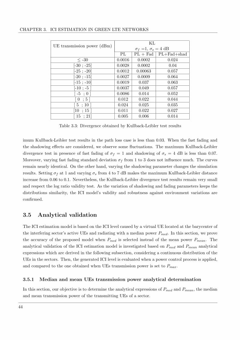
CHAPTER 3. ICI ESTIMATION IN GREEN LTE NETWORKS
UE transmission power (dBm)KL
σf =1, σs = 4 dBPL PL + Fad PL+Fad+shad
≤ -30 0.0016 0.0002 0.024
[-30 ; -25] 0.0028 0.0002 0.04
[-25 ; -20] 0.0012 0.00063 0.057
[-20 ; -15] 0.0027 0.0009 0.064
[-15 ; -10] 0.0019 0.037 0.063
[-10 ; -5 ] 0.0037 0.049 0.057
[ -5 ; 0 ] 0.0086 0.014 0.052
[ 0 ; 5 ] 0.012 0.022 0.044
[ 5 ; 10 ] 0.024 0.025 0.035
[10 ; 15 ] 0.011 0.022 0.027
[ 15 ; 21] 0.005 0.006 0.014
Table 3.3: Divergence obtained by Kullback-Leibler test results
imum Kullback-Leibler test results in the path loss case is less than 0.03. When the fast fading and
the shadowing effects are considered, we observe some fluctuations. The maximum Kullback-Leibler
divergence test in presence of fast fading of σf = 1 and shadowing of σs = 4 dB is less than 0.07.
Moreover, varying fast fading standard deviation σf from 1 to 3 does not influence much. The curves
remain nearly identical. On the other hand, varying the shadowing parameter changes the simulation
results. Setting σf at 1 and varying σs from 4 to 7 dB makes the maximum Kullback-Leibler distance
increase from 0.06 to 0.1. Nevertheless, the Kullback-Leibler divergence test results remain very small
and respect the log ratio validity test. As the variation of shadowing and fading parameters keeps the
distributions similarity, the ICI model’s validity and robustness against environment variations are
confirmed.
3.5 Analytical validation
The ICI estimation model is based on the ICI level caused by a virtual UE located at the barycenter of
the interfering sector’s active UEs and radiating with a median power Pmed. In this section, we prove
the accuracy of the proposed model when Pmed is selected instead of the mean power Pmean. The
analytical validation of the ICI estimation model is investigated based on Pmed and Pmean analytical
expressions which are derived in the following subsection, considering a continuous distribution of the
UEs in the sectors. Then, the generated ICI level is evaluated when a power control process is applied,
and compared to the one obtained when UEs transmission power is set to Pmax.
3.5.1 Median and mean UEs transmission power analytical determination
In this section, our objective is to determine the analytical expressions of Pmed and Pmean, the median
and mean transmission power of the transmitting UEs of a sector.
44
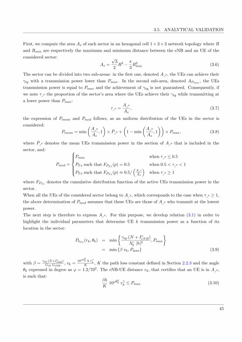
3.5. ANALYTICAL VALIDATION
First, we compute the area As of each sector in an hexagonal cell 1× 3× 3 network topology where R
and Rmin are respectively the maximum and minimum distance between the eNB and an UE of the
considered sector:
As =
√3
2R2 − π
3R2min (3.6)
The sector can be divided into two sub-areas: in the first one, denoted A, the UEs can achieve their
γtg with a transmission power lower than Pmax. In the second sub-area, denoted APmax , the UEs
transmission power is equal to Pmax and the achievement of γtg is not guaranteed. Consequently, if
we note τ the proportion of the sector’s area where the UEs achieve their γtg while transmitting at
a lower power than Pmax:
τ =AAs
, (3.7)
the expression of Pmean and Pmed follows, as an uniform distribution of the UEs in the sector is
considered:
Pmean = min
(AAs
, 1
)× P +
(1−min
(AAs
, 1
))× Pmax, (3.8)
where P denotes the mean UEs transmission power in the section of A that is included in the
sector, and:
Pmed =
Pmax when τ ≤ 0.5
PTx such that FPTx(p) = 0.5 when 0.5 < τ < 1
PTx such that FPTx(p) ≈ 0.5/(AAs
)when τ ≥ 1
where FPTx denotes the cumulative distribution function of the active UEs transmission power in the
sector.
When all the UEs of the considered sector belong to A, which corresponds to the case when τ ≥ 1,
the above determination of Pmed assumes that these UEs are those of A who transmit at the lowest
power.
The next step is therefore to express A. For this purpose, we develop relation (3.1) in order to
highlight the individual parameters that determine UE k transmission power as a function of its
location in the sector:
PkTx(rk, θk) = min
γtg.(N + IceNB)
Λck |h|2, Pmax
= min β vk, Pmax (3.9)
with β =γtg.(N+IceNB)GM GeNB
, vk =10ϕθ
2k h rγkK , K the path loss constant defined in Section 2.2.3 and the angle
θk expressed in degree as ϕ = 1.2/702. The eNB-UE distance rk, that certifies that an UE is in A,
is such that:βh
K10ϕθ
2k rγk ≤ Pmax (3.10)
45

CHAPTER 3. ICI ESTIMATION IN GREEN LTE NETWORKS
hence,
rk ≤ κmax10−ϕθ
2kγ (3.11)
where
κmax =
(K Pmaxβh
) 1γ
(3.12)
and is deviated by introducing κP such that,
κP =
(K P
β|h|2) 1γ
(3.13)
Consequently, A is determined as follows:
A =
∫ π3
−π3
∫ κmax10−ϕθ
2
γ
Rmin
r dr dθ
=κ2max
2ω1,π
3− π
3R2min (3.14)
where ω1,π3
is determined such that:
ω1,x =
∫ x
−x10− 2ϕ
γθ2dθ
=
√πγ
ϕLog(100)erf
(x
√ϕ
γLog(100)
)(3.15)
and ω1,π3≈ 1.5.
As the UEs are uniformly distributed in the network, their probability density function fUEs is constant
and:
fUEs(r, θ) =
1/As when τ < 1
1/A when τ ≥ 1
Consequently, the cumulative distribution function of the UEs transmission power is:
FPTx(p) = Prob(PTx ≤ p)= FV (
p
β)
=
∫∫A
fUEs(r, θ) r dr dθ
=fUEs
2
∫ π3
−π3
[κ2P 10
− 2ϕθ2
γ −R2min
]dθ (3.16)
=
(κ2P
2ω1,π
3− π
3R2min
)fUEs (3.17)
46

3.5. ANALYTICAL VALIDATION
(R∩s , θ∩s)(R∩′s
, θ∩′s)
ε′
ε
θ∩′s
θ∩s
Figure 3.8: Intersection between the sector’s limit and the boundary of A for τ ≥ 1, R∩s < R
When τ < 1, the mean value of the transmission powers of the UEs - in the sector only - in the As
area is, by definition:
P =1
A
∫ π3
−π3
∫ κmax10−ϕθ
2
γ
Rmin
βh
K10ϕθ
2rγ r dr dθ (3.18)
When τ ≥ 1, a large proportion of the UEs in the sector transmit at a lower power than Pmax. But
due to the eNB antenna radiation pattern directivity, some of the UEs in the sector can be outside
the A area.
It is therefore necessary to find the intersection, denoted ∩s, between the sector’s limit and the
boundary of A. The set ∩s contains two points whom polar coordinates are: θ∩s = ±π3 and
R∩s = κmax10−ϕ(π3 )2/γ .
If R∩s is higher than R (Figure 3.9), all the UEs in the sector transmit at a lower power than Pmax.
The mean UEs transmission power is then approximated from the computation of the mean UEs
transmission power over a third of disk of radius R - without limitation by Pmax, which leads to a
minor overestimation of Pmean:
Pmean =AsAo
∫ π3
−π3
∫ R
Rmin
1
Ao
βh
K10ϕθ
2rγ r dr dθ (3.19)
where
Ao =π
3
(R2 −R2
min
)(3.20)
47

CHAPTER 3. ICI ESTIMATION IN GREEN LTE NETWORKS
(R∩s , θ∩s)
R
Figure 3.9: Intersection between the sector’s limit and the boundary of A for τ ≥ 1, R∩s > R
If R∩s is lower than R (Figure 3.8), some UEs, in the upper and lower part of the sector, transmit at
Pmax. We denote ∩′s the intersection between the boundary of A and the circle of radius R. Then
∩′s contains two points whom polar coordinates are: R∩′s= R and θ∩′s
= ± γϕ log10
(κmaxR
).
We divide the sector into two parts:
1. the central one is bounded by −θ∩′s ≤ θ ≤ θ∩′sand Rmin ≤ r ≤ R. In this area of surface
Ac, the mean UEs transmission power is slightly overestimated by considering the extra-part,
denoted ε on Figure 3.8, beyond the sector’s limit.
2. the edge one, composed by the lower and upper parts of the sector, is bounded by θ < −θ∩′s or
θ > θ∩′sand Rmin ≤ r ≤ κmax10
−ϕθ2
γ . In this area of surface Ae, the mean UEs transmission
power is slightly underestimated because the extreme UEs locations in the sector, denoted ε′
on Figure 3.8, are not considered.
Thanks to the eNB antenna radiation pattern’s symmetry, the mean UEs transmission power Pmean
is therefore approximated by:
Pmean =2
Ac +Ae
∫ θ∩′s
0
∫ R
Rmin
βh
K10ϕθ
2
rγ r dr dθ +
∫ π3
θ∩′s
∫ κmax10−ϕθ
2
γ
Rmin
βh
K10ϕθ
2
rγ r dr dθ
(3.21)
where
Ac =(R2 −R2
min
)θ∩′s
and
Ae =κ2max
2
(ω1,π
3− ω1,θ
∩′s
)−R2
min
(π3− θ∩′s
)48

3.5. ANALYTICAL VALIDATION
Finally, the mean value of the transmission powers of the UEs - in the sector only - is obtained after
derivations:
Pmean =
P1 when τ ≤ 1
P2 when τ > 1 and R∩s ≥ RP3 when τ > 1 and R∩s < R
where,
P1 =1
A
βh
K(γ + 2)
(κγ+2max ω1,π
3−Rγ+2
min ω2,π3
)τ + (1− τ) Pmax
P2 =1
A
βh
K(γ + 2)
(κγ+2max ω1,π
3−Rγ+2
min ω2,π3
)τ + (1− τ) Pmax
and
P3 =1
Ac +Ae
βh
K(γ + 2)
((Rγ+2 −Rγ+2
min
)ω2,θ
∩′s+ κγ+2
max
(ω1,π
3− ω1,θ
∩′s
)−Rγ+2
min
(ω2,π
3− ω2,θ
∩′s
))As for ω1,x, we introduce ω2,x given with the imaginary error function erfi3 as:
ω2,x =
∫ x
−x10ϕθ
2dθ
=
√π
ϕ log10
erfi(x√ϕ log10
)(3.22)
and ω2,π3≈ 5.03.
In the same way, the median value of the transmission powers of the UEs - in the sector only - is
obtained after derivations:
Pmed =
Pmax when τ ≤ 0.5
βhK
[2Asω1, π3
(0.5 +
πR2min
3As
)] 2γ
when 0.5 < τ < 1
βhK
[2ω1, π3
(0.5 As
A+
πR2min
3A
)] 2γ
when τ ≥ 1
Next subsection is dedicated to the results provided by the analytical determination of Pmean and
Pmed.
3.5.2 Simulation results
The purpose of this subsection is to check that: 1) the empirical computations of Pmean and Pmed,
determined from the NUE UEs transmission powers, are close to their analytical computations issued
from the previous subsection, and 2) the use of Pmed instead of Pmean for the virtual interfering UE
transmission power leads to a more accurate estimation of the ICI and the UEs stable transmission
3erfi is the imaginary error function: erfi(z) = −i erf(iz)
49
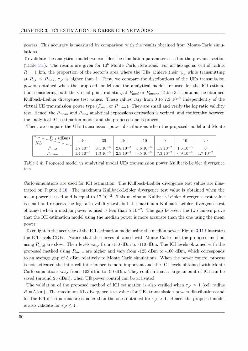
CHAPTER 3. ICI ESTIMATION IN GREEN LTE NETWORKS
powers. This accuracy is measured by comparison with the results obtained from Monte-Carlo simu-
lations.
To validate the analytical model, we consider the simulation parameters used in the previous section
(Table 3.1). The results are given for 106 Monte Carlo iterations. For an hexagonal cell of radius
R = 1 km, the proportion of the sector’s area where the UEs achieve their γtg while transmitting
at Pe,k ≤ Pmax, τ is higher than 1. First, we compare the distributions of the UEs transmission
powers obtained when the proposed model and the analytical model are used for the ICI estima-
tion, considering both the virtual point radiating at Pmed or Pmean. Table 3.4 contains the obtained
Kullback-Leibler divergence test values. These values vary from 0 to 7.3 10−2 independently of the
virtual UE transmission power type (Pmed or Pmean). They are small and verify the log ratio validity
test. Hence, the Pmean and Pmed analytical expressions derivation is verified, and conformity between
the analytical ICI estimation model and the proposed one is proved.
Then, we compare the UEs transmission power distributions when the proposed model and Monte
XXXXXXXXXXKLPe,k (dBm)
-40 -30 -20 -10 0 10 20
Pmed 1.7 10−5 3.4 10−3 2.8 10−3 5.6 10−3 1.5 10−2 1.5 10−3 0Pmean 1.4 10−3 1.3 10−3 2.3 10−3 9.5 10−3 7.3 10−2 6.9 10−2 1.7 10−2
Table 3.4: Proposed model vs analytical model UEs transmission power Kullback-Leibler divergencetest
Carlo simulations are used for ICI estimation. The Kullback-Leibler divergence test values are illus-
trated on Figure 3.10. The maximum Kullback-Leibler divergence test value is obtained when the
mean power is used and is equal to 17 10−2. This maximum Kullback-Leibler divergence test value
is small and respects the log ratio validity test, but the maximum Kullback-Leibler divergence test
obtained when a median power is used is less than 5 10−2. The gap between the two curves prove
that the ICI estimation model using the median power is more accurate than the one using the mean
power.
To enlighten the accuracy of the ICI estimation model using the median power, Figure 3.11 illustrates
the ICI levels CDFs. Notice that the curves obtained with Monte Carlo and the proposed method
using Pmed are close. Their levels vary from -130 dBm to -110 dBm. The ICI levels obtained with the
proposed method using Pmean are higher and vary from -125 dBm to -100 dBm, which corresponds
to an average gap of 5 dBm relatively to Monte Carlo simulations. When the power control process
is not activated the inter-cell interference is more important and the ICI levels obtained with Monte
Carlo simulations vary from -103 dBm to -90 dBm. They confirm that a large amount of ICI can be
saved (around 25 dBm), when UE power control can be activated.
The validation of the proposed method of ICI estimation is also verified when τ ≤ 1 (cell radius
R = 5 km). The maximum KL divergence test values for UEs transmission powers distributions and
for the ICI distributions are smaller than the ones obtained for τ > 1. Hence, the proposed model
is also validate for τ ≤ 1.
50

3.5. ANALYTICAL VALIDATION
−40 −30 −20 −10 0 10 20 300
0.02
0.04
0.06
0.08
0.1
0.12
0.14
0.16
0.18
UE Transmission power (dBm)
Kullb
ack−
Leib
ler
test
Proposed method with median
Proposed method with mean
Figure 3.10: Monte Carlo vs Analytical model UEs transmission power Kullback Leiber test for R=1km
Figure 3.12 and 3.13, respectively, show the controlled UEs transmission powers obtained as a func-
tion of the ICI level computation methods for τ > 1 and τ ≤ 1. In both cases, we note that the
CDFs of the UEs transmission powers when the ICI is estimated with the proposed model and its
analytical expression are close independently of the virtual UE transmission power type. However,
the CDF obtained when the virtual UE transmits at Pmed is closer, and proves that using the median
power is more accurate. The UEs transmission power CDFs are lower bounded with the CDF of UEs
transmission power computed in noise limited network, and upper bounded with the CDF of the UEs
transmission power computed when the ICI is set at its maximum, considering that the power control
is not activated for the interferers. For macro cells with a radius R = 5 km, the UEs transmission
powers vary between -10 dBm and Pmax. This is due to the path loss, where at a far distance from
the eNB, the UEs should transmit at a higher power to achieve their QoS.
51

CHAPTER 3. ICI ESTIMATION IN GREEN LTE NETWORKS
−135 −130 −125 −120 −115 −110 −105 −100 −95 −900
0.1
0.2
0.3
0.4
0.5
0.6
0.7
0.8
0.9
1Intercell interference power CDF
Inter−cell interference Ic
eNB (dBm)
pro
b (
Ic eN
B <
x)
With PC − Prop. meth (med)
With PC − Prop. meth (mean)
With PC − Monte−Carlo simulations
Wo PC − Monte Carlo simulations
Figure 3.11: ICI cumulative distribution function for R=1 km
3.6 Conclusion
Power control applied on the uplink to the UE transmission power, based on a SINR threshold, dras-
tically reduces the inter-cell interference. This reduction comes at the expense of a higher complexity
in the derivation of ICI level. The method we proposed to estimate the inter-cell interference is less
heavy and greedy in computation than the classical Monte Carlo method. Actually, it does not drop
users in the interfering sectors as Monte Carlo method requires. In this chapter, we have shown that a
single virtual UE, situated at the barycenter of each of the concerned interfering sectors, allows us to
precisely evaluate the ICI. This virtual UE interferer transmits at the median power of the interfering
sector’s active UEs, assuming that all neighboring cells behave the same way than the central cell.
This equivalent median power creates, in any environment, an inter-cell interference at the central eNB
equivalent to that derived with random interfering users obtained from Monte Carlo simulations. An
analytical model was also derived to evaluate this virtual UE median power transmission. It allowed
an accurate ICI level estimation with an even lower computational complexity, and therefore reduce
the planning and evaluation simulators complexity.
52

3.6. CONCLUSION
−40 −30 −20 −10 0 10 20 300
0.1
0.2
0.3
0.4
0.5
0.6
0.7
0.8
0.9
1
UE transmission power Pk
Tx
c (dBm)
pro
b (
Pk
Tx
c <
x)
Noise limited network
With PC − Prop. meth (med)
With PC − Prop. meth, anal. res. (med)
With PC − Monte−Carlo simulations
With PC − Prop. meth (mean)
With PC − Prop. meth, anal. res. (mean)
Wo PC − Prop. meth
Wo PC − Monte Carlo simulations
Figure 3.12: UEs transmission power for R=1 km
−10 −5 0 5 10 15 200
0.1
0.2
0.3
0.4
0.5
0.6
0.7
0.8
0.9
1
UE Transmission power pk
Tx
c (dBm)
pro
b (
Pk
Tx
c <
x)
Noise limited network
With PC − Prop. meth (med)
With PC − Monte−Carlo simulations
With PC − Prop. meth (mean)
Wo PC − Monte Carlo simulations
Figure 3.13: UEs transmission power for R=5 km
53

CHAPTER 3. ICI ESTIMATION IN GREEN LTE NETWORKS
54

Chapter 4
Dimensioning outage probability
Upper-bound depending on RRM in
Uplink LTE networks
Part of this chapter was published in IEEE GLOBECOM 20131
RADIO resource management aims at maximizing the system performances by allocating
efficiently the limited number of RBs. This maximization is reached while the number of
allocated RBs per cell is adapted with: i) the network’s load and ii) the user’s required QoS.
These two parameters should be considered while determining the maximum number of allocated RBs
per cell, corresponding to the allocated bandwidth per cell. Within this framework, the dimensioning
outage probability is defined as the probability that a user is not served due to a lack of RBs in the
network. In this chapter, we propose an analytical model that estimates the dimensioning outage
probability upper bound which helps system planners to evaluate and adapt the allocated bandwidth
to each cell. The dimensioning outage probability upper bound is evaluated as a function of the used
RB allocation algorithm. This analytical model applies to the cases of single and multiple user’s QoS
classes and is also extended to the case of MIMO systems.
1F.Z. Kaddour, P. Martins, L. Decreusefond, E. Vivier and L. Mroueh, “Outage probability upper’s bound in uplinkLong Term Evolution networks with multi QoS users classes ”, in proceedings of IEEE Global Communications conference(GLOBECOM), Atlanta, USA, December, 2013.
55

CHAPTER 4. DIMENSIONING OUTAGE PROBABILITY UPPER BOUND DEPENDING ON RRM
4.1 Introduction
Wireless cell planning aims at providing a proper radio network configuration, given in terms of: net-
work coverage, offered QoS, capacity, deployed equipments, etc. Usually, the cell network planners
study the area and create a database with the geographic information. They analyze the behavior of
the population in the area and the required QoS. For these reasons, they require techniques to estimate
the network configuration and to evaluate the required bandwidth that should be allocated to each
cell or sector. Each allocated bandwidth consists of a limited number of RBs. In order to allocate RBs
to cell’s users, RRM entity takes into account their required QoS and their channel conditions. In this
chapter, a user is considered in outage if there is not enough available RBs to serve and satisfy its QoS.
Most cells are considered in theory as hexagonal grids, but in reality and for severals factors, it
is not the case. With the help of point processes, that consider the network’s spatial distribution as
random, we study the statistical behavior of the network configuration. It helps the cell planners to
study an average behavior of the network. Our objective is to compute the upper bound of the dimen-
sioning outage probability and to estimate the required bandwidth for the network. This problem was
previously studied for the downlink OFDMA network in [66]. Our contribution lies in computing this
upper bound in the uplink of LTE networks, considering single and multiple QoS classes according to
the RB allocation policy applied by the RRM entity. We consider two RB allocation algorithms: (i)
the fair RB allocation algorithm which uniformly allocates RBs to users and (ii) the opportunistic RB
allocation algorithm which allocates RBs to the users benefiting from the best channel conditions. We
focus on the dimensioning problem that determines the necessary RBs used for transmission in order
to achieve the target capacity. The user’s throughput is computed by means of the Shannon capacity.
However, the considered RB allocation algorithms define the users’ selection methodology without
specifying the adjacency constraint of the allocated RBs. Then, the proposed analytical model pre-
sented in this chapter can be used for dimensioning LTE release 8 and LTE-A networks. In addition,
the analytical model is developed for the diversity and multiplexing gains in MIMO systems.
Due to their largest arsenal of results, Poisson point processes are widely used to characterize the
statistical behavior over many spatial random realizations of a network. Moreover, they are more
tractable and simple to use than other point process models.
In our work, the total required number of RBs is assimilated to a marked Poisson point process.
Only the first and second mathematical moments of this marked Poisson point process are necessary
to evaluate the upper bound of the dimensioning outage probability.
In Section 4.2 the main assumptions that are used for the computation of the dimensioning outage
probability’s upper bound are discussed. Dimensioning outage probability upper bound in SISO
systems is computed in Section 4.3. It is extended to MIMO systems in Section 4.4. In Section 4.5,
the obtained numerical results and the proposed model validation are discussed.
56

4.2. ASSUMPTIONS FOR DIMENSIONING OUTAGE PROBABILITY UPPER BOUND DERIVATION
4.2 Assumptions adopted for the computation of the dimensioning
outage probability’s upper bound
For dimensioning purpose, we are interested in evaluating and computing the upper bound Psup of the
dimensioning outage probability Pout, that there is not enough available resources NRB in the network
to serve and satisfy the QoS required by all the active users.
We define ϕUE the set of all active users positions in the cell C with cardinality | ϕUE |= NUE . The
throughput corresponding to the user’s required QoS is noted C0. Then, each user k at position x in
the cell C needs Nk(x) RBs to satisfy its target throughput C0. Consequently, the total number N of
RBs to serve and satisfy all the users in the cell C is:
N =∑
k∈ϕUE
Nk(x)
If the necessary number of RBs per cell, N, is higher than the number of available RBs in the cell,
NRB, then the system is in outage. The dimensioning outage probability is then expressed as:
Pout = Prob
(∫Ndϕ ≥ NRB
)(4.1)
In this Chapter, the Shannon capacity theorem is used for the throughput computation. If γk is the
average SINR of the user k over the RBs (by considering average shadowing and fading effects), then
its number of required RBs to achieve its target throughput C0 is expressed as:
Nk =
⌈C0
Ck
⌉(4.2)
where Ck = W log2(1 + γk) is the average Shannon capacity of the user k in one RB of a bandwidth
W . For computation simplicity, we work on the assumptions that:
Assumption 4.1 The cell C is circular, with radius R and with the eNB at its center. The eNB
antenna is assumed to be omnidirectional.
Assumption 4.2 Each user is allowed to transmit only if its SINR is higher than a signal to inter-
ference plus noise ratio threshold γmin. This means that the maximum number of RBs allowed to a
UE, is upper bounded by:
Nmax =
⌈C0
W log2(1 + γmin)
⌉(4.3)
Assumption 4.3 The power control is not taken into account. Each user k transmits at its maximum
power Pmax over its whole allocated RBs. In the SC-FDMA technique the total mobile’s transmission
power is equally shared over the allocated RBs. Then,
PkTx =Pmax
Nmax∀ k ∈ ϕUE
57

CHAPTER 4. DIMENSIONING OUTAGE PROBABILITY UPPER BOUND DEPENDING ON RRM
In this chapter, PkTx is denoted Pt as it is supposed to be constant for all users.
This assumption leads to an under estimation of the user’s SINR. Actually, users that will be allocated
less than Nmax RBs will benefit from a margin in their SINR estimation. Consequently, they will
achieve a higher throughput than C0.
In addition, each user k is marked by the uplink scheduler decision noted z. This decision selects
(z = 1) or not (z = 0) the user k to transmit data on RBs, with regards to assumption 4.2. Since the
mark z, z ∈ Z = 0, 1, is independent from one user to another, then the number of allocated RBs
Nk(x, z) is considered as a marked Poisson point process.
Assumption 4.4 User k at position x is served Nk(x) RBs if and only if it is selected by the scheduler.
Fair RB allocation and opportunistic RB allocation algorithms are considered.
These assumptions, which are quite reasonable, are commonly used to simplify the mathematical
computation.
4.3 Dimensioning outage probability upper bound in SISO systems
In SISO systems, we consider that the radio channel is affected by shadowing. Hence, we state the
following assumptions:
Assumption 4.5 The channel gain depends on each user’s position x and on the shadowing gain gs
equal to 1S , where the linear values y of S follow a log-normal distribution with mean µs and a standard
deviation σs as:
ps(y) =ξ
σsy√
2πexp
(−(10 log10 y − µs)2
2σ2s
)(4.4)
where, ξ = 10/ ln 10
The analytical model of the dimensioning outage probability upper bound is detailed in the following
subsection for single and multiple user’s QoS classes.
4.3.1 Single users’ QoS class in SISO systems
When the assumptions cited before are considered, the required number of RBs that should be allo-
cated to each user k localized at position x in order to achieve its target throughput C0, is given as a
function of the channel conditions and the RRM decision as follows:
Nk(x, y, z) =
⌈C0
W log2
(1+
PtPL(x)
ηy
)⌉z (4.5)
=
C0
W log2
(1+
PtK
ηy‖x‖β
) z
(4.6)
58

4.3. DIMENSIONING OUTAGE PROBABILITY UPPER BOUND IN SISO SYSTEMS
where PL(x) is the path loss when user k is localized at position x; K and β are respectively the path
loss constant and the path loss exponent defined in Section 2; η is the sum of the thermal noise N in
the considered bandwidth and the average inter-cell interference level received at the eNB in one RB
IceNB. The marks y and z represent respectively the shadowing and the RRM decision’s marks.
Since the marks are independent, Nk(x, y, z) is a Poisson point process on R3 of intensity Λ(x) ⊗ps(y)dy ⊗ p(z)dz. We compute the upper bound Psup of the dimensioning outage probability Pout
for: (i) the fair RB allocation algorithm: P SISOsup,Fair, and (ii) the opportunistic RB allocation algorithm:
P SISOsup,Opp.
Fair RB allocation algorithm:
The fair RB allocation algorithm allocates RBs to all users, whatever their channel conditions. Hence,
the probability that a user will be selected by the scheduler for transmission follows a uniform distri-
bution:
p(z) =1
NUE(4.7)
Studying the network behavior statistically, we consider that the number of UEs in the cell NUE can
be expressed as:
NUE =ρ
νπR2
where, ρ and 1ν are respectively the surface density and service mean time. According to the concen-
tration inequality, we should compute the first and the second moment of the Poisson point process,
using the Campbell formula (Theorem 2.1), as:
mN =
∫N(x, y, z) ps(y)dy p(z)dz dΛ(x) (4.8)
and
vN =
∫N2(x, y, z) ps(y)dy p(z)dz dΛ(x) (4.9)
We assume γj to be the SINR threshold, j being the user’s required number of RBs to achieve its
target throughput C0, with:
γj = 2C0/(jW ) − 1 for j = 1, · · · , Nmax − 1 and γ0 =∞
and we define Aj the area which contains the users that require at most j RBs to satisfy their target
throughput C0. The area Aj can be determined as follows:
Aj =
∫C×R+×Z
1y‖x‖β≤PtK/ηγj ps(y)dy p(z)dz dx
=
∫C×R+×Z
p(y‖x‖β ≤ γj
)p(z)dz dy dx (4.10)
59

CHAPTER 4. DIMENSIONING OUTAGE PROBABILITY UPPER BOUND DEPENDING ON RRM
where γj = PtKηγj
.
After a tedious but straightforward integration by parts, detailed in Appendix 4.A.1, we obtain :
Aj = νρR2 exp (2/ζ + 2αj/ζ)Φ(ζ lnR− 2/ζ − αj) + ν
ρΦ(αj − ζ lnR) (4.11)
with Φ the normal cumulative distribution function2, and the variables αj and ζ expressed respectively,
as:
αj =1
σs(10 log10(γj)− µs)
and
ζ =10β
σs ln 10
Then, the first and second moments of Nk(x, y, z) in the fair RB allocation algorithm case can respec-
tively be written as a function of Aj as:
mSISONFair
=ρ
ν
Nmax−1∑j=1
j(Aj −Aj−1) +ρ
νNmax(πR2 −ANmax−1) (4.12)
and
vSISONFair
=ρ
ν
Nmax−1∑j=1
j2(Aj −Aj−1) +ρ
νN2
max(πR2 −ANmax−1) (4.13)
Using the concentration inequality, the upper bound of the dimensioning outage probability in case of
a fair RB allocation algorithm is:
Prob
(∫Ndϕ ≥ NRB
)≤ P SISO
sup,Fair
where,
P SISOsup,Fair = exp
(−vSISONFair
N2max
g
((α−1)mSISO
NFairNmax
vSISONFair
))(4.14)
and g(t) = (1 + t) ln(1 + t)− t.Using the same methodology, the dimensioning outage probability upper bound in SISO systems using
an opportunistic RB allocation algorithm is given in the next paragraph.
Opportunistic RB allocation algorithm:
The opportunistic RB allocation algorithm seeks to maximize the total throughput of the cell C.
Hence, it allocates each RB to the user with the highest SINR. Then, the probability of selecting a
user depends on its channel conditions, given with the path loss and shadowing effects.
2the normal cumulative distribution function is expressed as: Φ = 12
+ 12erf( x√
2)
60
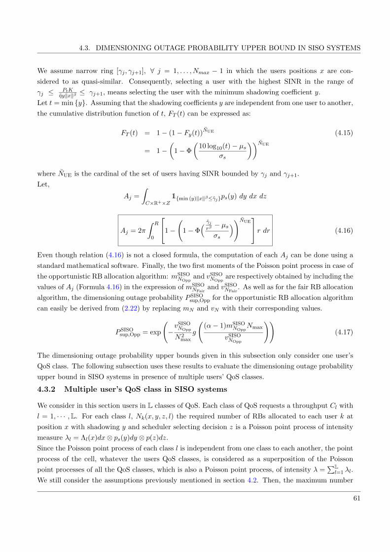
4.3. DIMENSIONING OUTAGE PROBABILITY UPPER BOUND IN SISO SYSTEMS
We assume narrow ring [γj , γj+1], ∀ j = 1, . . . , Nmax − 1 in which the users positions x are con-
sidered to as quasi-similar. Consequently, selecting a user with the highest SINR in the range of
γj ≤ PtKηy‖x‖β ≤ γj+1, means selecting the user with the minimum shadowing coefficient y.
Let t = min y. Assuming that the shadowing coefficients y are independent from one user to another,
the cumulative distribution function of t, FT (t) can be expressed as:
FT (t) = 1− (1− Fy(t))NUE (4.15)
= 1−(
1− Φ
(10 log10(t)− µs
σs
))NUE
where NUE is the cardinal of the set of users having SINR bounded by γj and γj+1.
Let,
Aj =
∫C×R+×Z
1min (y)‖x‖β≤γjps(y) dy dx dz
Aj = 2π
∫ R
0
1−(
1− Φ( γjrβ− µsσs
))NUE r dr (4.16)
Even though relation (4.16) is not a closed formula, the computation of each Aj can be done using a
standard mathematical software. Finally, the two first moments of the Poisson point process in case of
the opportunistic RB allocation algorithm: mSISONOpp
and vSISONOpp
are respectively obtained by including the
values of Aj (Formula 4.16) in the expression of mSISONFair
and vSISONFair
. As well as for the fair RB allocation
algorithm, the dimensioning outage probability P SISOsup,Opp for the opportunistic RB allocation algorithm
can easily be derived from (2.22) by replacing mN and vN with their corresponding values.
P SISOsup,Opp = exp
(−vSISONOpp
N2max
g
((α− 1)mSISO
NOppNmax
vSISONOpp
))(4.17)
The dimensioning outage probability upper bounds given in this subsection only consider one user’s
QoS class. The following subsection uses these results to evaluate the dimensioning outage probability
upper bound in SISO systems in presence of multiple users’ QoS classes.
4.3.2 Multiple user’s QoS class in SISO systems
We consider in this section users in L classes of QoS. Each class of QoS requests a throughput Cl with
l = 1, · · · ,L. For each class l, Nk(x, y, z, l) the required number of RBs allocated to each user k at
position x with shadowing y and scheduler selecting decision z is a Poisson point process of intensity
measure λl = Λl(x)dx⊗ ps(y)dy ⊗ p(z)dz.Since the Poisson point process of each class l is independent from one class to each another, the point
process of the cell, whatever the users QoS classes, is considered as a superposition of the Poisson
point processes of all the QoS classes, which is also a Poisson point process, of intensity λ =∑L
l=1 λl.
We still consider the assumptions previously mentioned in section 4.2. Then, the maximum number
61

CHAPTER 4. DIMENSIONING OUTAGE PROBABILITY UPPER BOUND DEPENDING ON RRM
of RBs allocated to each user of class l is given by:
Nl,max =
⌈Cl
W log2(1 + γmin)
⌉The upper bound of the dimensioning outage probability P SISO
sup,QoS is then,
P SISOsup,QoS = exp
(− vN
N2max
g
((α− 1)mN Nmax
vF
))(4.18)
where, Nmax is the maximum number of RBs allowed in all the QoS classes,
Nmax = maxk
Nk,max (4.19)
and mN and vN are respectively the first and the second moment of the Poisson point process expressed
as:
mN =∑L
l=1mN,l (4.20)
vN =∑L
l=1 vN,l, (4.21)
with mN,l and vN,l the first and second moments of the Poisson point process of each class l. They
can be driven from the single user’s QoS class in SISO system study as a function of the RB allocation
algorithm chosen, as detailed in the previous section.
In the following section, the same methodology as for the point-to-point SISO case is used to derive
the dimensioning outage probability upper bound in a MIMO system, as a function of the RRM
algorithm.
4.4 Dimensioning outage probability upper bound computation in
MIMO systems
In this section, we consider the MIMO system defined in Chapter 2, Section 2.3.2. Let nt be the
number of transmit antennas at the transmitter side (i.e. the UE) and nr be the number of receive
antennas at the receiver side (i.e. the eNB). We assume that the UE experiences the same path
loss and the same shadowing over all its antennas. Actually, in MIMO systems, the effect of the
fading is more relevant than the shadowing one as when the antennas are sufficiently separated at
each device, the fading coefficients can be considered as different over all the paths. Therefore, the
following assumption is added to assumptions 4.1, 4.2, 4.3 and 4.4.
Assumption 4.6 The channel gain depends only on the user’s position x and the Rayleigh fast fading
effect.
62

4.4. DIMENSIONING OUTAGE PROBABILITY UPPER BOUND COMPUTATION IN MIMO SYSTEMS
The shadowing effects are not considered here and the interferences are assumed to be negligible
compared to the noise. We denote by H the channel matrix containing all the fading coefficients
between the transmit and receive antennas.
One of the main advantages of MIMO systems is the possibility to multiplex min(nt, nr) data streams
in the same RB. Furthermore, MIMO systems can be used to improve the system’s reliability by
exploiting the spatial diversity of transmission. In the following, we consider two different MIMO
strategies: i) the first one extracts the diversity of a MIMO system, ii) the second one aims to multiplex
min(nt, nr) streams on the same RB. For these two strategies, an dimensioning outage probability
upper bound is evaluated when using a fair RB allocation algorithm, and then an opportunistic one.
4.4.1 MIMO diversity gain with fair RB allocation algorithm
In the first considered scheme, each UE selects the antenna that experiences the best channel conditions
in order to achieve a high data rate and to transmit its data. Hence, the UE chooses the path having
the maximal fading magnitude among the ntnr possible fading paths, i.e.,
|h∗|2 = max1≤i≤nt,1≤j≤nr
|hi,j |2.
Let u = |h∗|2 be the maximal fading magnitude. Each coefficient hi,j follows a complex Gaussian
distribution hi,j ∼ CN (0, 1) and has a magnitude |hi,j |2 that is exponentially distributed. Hence, u
is the maximal value of ntnr random variables that are exponentially distributed and its cumulative
distribution function is such that,
FU (u) = (1− e−u)ntnr
Consequently, the probability distribution function of u is such that,
pU (u) =dFU (u)
du= ntnr(1− e−u)ntnr−1 e−u
The SINR experienced by the UE is then expressed as:
γ =PtKu
η‖x‖β
The number of allocated RBs for each UE k at position x is a Poisson point process marked with the
maximum fading coefficient u and the scheduler decision z as:
Nk(x, u, z) =
⌈C0
W log2(1 + PtKuη‖x‖β )
⌉z (4.22)
For fair RB allocation algorithm, all UEs are served with equal probability and hence p(z) = 1NUE
.
Let γj be the SINR threshold that allows each UE to achieve its target throughput C0 with j the
number of required RBs by each UE. We define γj = 2C0jW − 1 for j = 1, . . . , Nmax− 1 and let γ0 =∞.
63

CHAPTER 4. DIMENSIONING OUTAGE PROBABILITY UPPER BOUND DEPENDING ON RRM
With assumption 4.2 we obtain:
PtKu
η‖x‖β ≥ γmin ⇒‖x‖βu≤ PtK
γminη
and PtKγminη
= γmin.
The area that contains the users which need j RBs are defined as follows:
Aj =
∫C×R+×[0,1]
1 ‖x‖βu≤γj pu(u) du dx p(z) dz
where γj = PtKγj η
. Then, by considering the polar coordinate system, the areas Aj ∀ j = 1, . . . , Nmax− 1
can be expressed as:
Aj = 1NUE
∫ R
0
∫ 2π
0
∫ +∞
rβ
γj
pu(u)du rdrdθ
= 1NUE
∫ R
0
∫ 2π
0
[1− FU
(rβ
γj
)]rdrdθ (4.23)
After some simplification,
Aj = 1NUE
[πR2 − 2π
∫ R
0r
(1− e−
rβ
γj
)ntnrdr
](4.24)
Using the Aj expression, we can compute the first and second moments mMIMON(Fair,Div)
and vMIMON(Fair,Div)
of the Poisson point process of the required number of allocated RBs when a fair RB allocation
algorithm is used in diversity gain MIMO systems, with the expressions of mSISONFair
and vSISONFair
The
corresponding PDiv,MIMOsup,Fair , the dimensioning outage probability upper bound in case of diversity gain
in MIMO systems using a fair RB allocation algorithm can, then, be derived from the concentration
inequality theorem (2.22)
PDiv,MIMOsup,Fair = exp
(−vMIMON(Fair,Div)
N2max
g
((α− 1)mMIMO
N(Fair,Div)Nmax
vMIMON(Fair,Div)
))(4.25)
4.4.2 MIMO multiplexing gain with fair RB allocation algorithm
We assume that the channel conditions are not known at the transmitter side. Consequently, the
transmission power is equally shared over the nt antennas. However, the receiver has a full channel
knowledge and uses a maximum likelihood optimal decoder. The channel capacity depends on the
eigen-values of the matrix HH†. Let HH† = UDU† be the eigen-value decomposition of HH† where
U is an unitary matrix and D is the diagonal matrix with non zero diagonal terms µ1, µ2, . . . , µm
entries with m = min(nt, nr) and µ1 ≤ µ2 ≤ . . . ≤ µm. In this case, the capacity of the MIMO channel
64

4.4. DIMENSIONING OUTAGE PROBABILITY UPPER BOUND COMPUTATION IN MIMO SYSTEMS
is such that,
C = log2 det(Int +
PtK
ntη‖x‖βHH†
)or equivalently,
C = log2
m∏i=1
(1 +
PtKµintη‖x‖β
)Let Ctot, be the total throughput required to transmit the streams on each transmitting antenna. The
number of required RBs per UE k at position x to reach Ctot is then:
Nk(x, µ, z) =
Ctot
W log2(∏mi=1(1 + PtKµi
ntη‖x‖β ))
z (4.26)
For dimensioning stress, we aim at over estimating the number of RBs and for this purpose, we consider
the dimensioning over the antenna that needs the highest number of RBs. Since the singular values
are ordered, we can find the maximum number of RBs that should be allocated to a UE k to satisfy
its target throughput Ctot such that:
Nk(x, µ, z) ≥
Ctot
Wm log2
(1 + PtKµ1
ntη‖x‖β
) z (4.27)
The cumulative distribution function Fµ1(µ) of the smallest eigen-value µ1 is computed for a general
case nt × nr MIMO and a special case of 2× 2 MIMO systems in the following paragraphs.
General case: nt × nr MIMO system
The entries of the matrix H follow a Gaussian distribution and the joint distribution of the order
eigen-values of the Wishart matrix HH† are known from [67] and are given by:
p(µ1,...,µm)(µ1, . . . , µm) = k−1nt,nr
m∏i=1
µ|nt−nr|i
∏i<j
(µi − µj)2e−∑mi=1 µi
where knt,nr is a normalization constant. The distribution of the smallest eigen-value µ1 can be
deduced by marginalizing over the variables µ2, . . . , µm i.e.
pµ1(µ1) =
∫Vp(µ1, . . . , µm)dµ2 . . . dµm
where V = 0 ≤ µ1 ≤ . . . µm ≤ ∞. The cumulative distributive function can be then deduced as,
Fµ1(µ) =
∫ µ
0pµ1(µ1)dµ1.
65

CHAPTER 4. DIMENSIONING OUTAGE PROBABILITY UPPER BOUND DEPENDING ON RRM
Then, the areas Aj are:
Aj =
∫θ
∫r
∫z
∫µ1
1 ‖x‖βµ1≤γMIMO
j
pµ1(µ1)dµ1p(z)dzrdrdθ
where γMIMOj = PtK
ntγMIMOj
with γMIMOj = 2
CtotmjW − 1 and p(z) is the probability that a UE is served,
which is equal to 1NUE
for a fair scheduling algorithm. Then,
Aj =1
NUE
∫θ
∫r
∫ +∞
rβ
γMIMOj
pµ1(µ1)dµ1rdrdθ,
=1
NUE
∫θ
∫r
[1− Fµ1
(rβ
γMIMOj
)]rdrdθ
After some mathematical derivations we obtain:
Aj = 1NUE
[πR2 − 2π
∫ R
0Fµ1
(rβ
γMIMOj
)rdr
](4.28)
Application to the 2× 2 MIMO case
We specify our results to the 2× 2 MIMO case. In this configuration, two streams can be transmitted
simultaneously in each RB. The joint distribution of the eigen-values is such that,
p(µ1,µ2)(µ1, µ2) = (µ1 − µ2)2e−(µ1+µ2)
The distribution of the smallest eigen-value µ1 can be deduced by marginalization,
pµ1(µ1) =
∫ ∞µ1
p(µ1, µ2)dµ2.
After some simplification, this gives,
pµ1(µ1) = 2e−2µ1
and the cumulative distribution function Fµ1(µ1) is such,
Fµ1(µ1) =
∫ µ1
0pµ1(x)dx = 1− e−2µ1
Then, the areas Aj are:
Aj =
∫θ
∫r
∫z
∫µ1
1 ‖x‖βµ1≤γMIMO
j
pµ1(µ1)dµ1p(z)dzrdrdθ
66

4.4. DIMENSIONING OUTAGE PROBABILITY UPPER BOUND COMPUTATION IN MIMO SYSTEMS
Then,
Aj =1
NUE
∫θ
∫r
∫ +∞
rβ
γMIMOj
pµ1(µ1)dµ1rdrdθ,
=1
NUE
∫θ
∫r
[1− Fµ1
(rβ
γMIMOj
)]rdrdθ
After some mathematical derivations we obtain:
Aj = 1NUE
[πR2 − 2π
∫ R
0
(1− e
−2 rβ
γMIMOj
)rdr
](4.29)
where γMIMOj = PtK
2γMIMOj
with γMIMOj = 2
Ctotj2W − 1. Then, the dimensioning outage probability upper
bound PMux,MIMOsup,Fair in case of MIMO multiplexing gain using a fair RB allocation algorithm is deduced
from the concentration inequality theorem (2.22) as:
PMux,MIMOsup,Fair = exp
(−vMIMON(Fair,Mux)
N2max
g
((α− 1)mMIMO
N(Fair,Mux)Nmax
vMIMON(Fair,Mux)
))(4.30)
The first and second moments mMIMON(Fair,Mux)
and vMIMON(Fair,Mux)
of the considered Poisson point process are
computed as a function of the areas Aj , using the expression of mSISONFair
and vSISONFair
.
4.4.3 MIMO diversity gain with opportunistic RB allocation algorithm
The opportunistic RB allocation algorithm serves first the user that experiences the best channel con-
ditions over all active users. This algorithm, when combined with the MIMO diversity technique that
we described in Subsection 4.4.1, serves the UE, denoted UE k∗, having the best channel magnitude
among NUEntnr random exponentially distributed values, such that:
k∗ = arg max1≤k≤NUE
[max
1≤i≤nt,1≤j≤nr| h(k)
i,j |2].
Then, the cumulative distribution function of the selected UE channel becomes:
FU∗(u∗) = (1− e−u∗)NUEntnr
and its probability distribution function is such that,
pU∗(u∗) = NUEntnr(1− e−u
∗)NUEntnr−1e−u
∗(4.31)
67

CHAPTER 4. DIMENSIONING OUTAGE PROBABILITY UPPER BOUND DEPENDING ON RRM
Similar derivation as in Subsection 4.4.1 can be repeated and the areas Aj become
Aj = πR2 − 2π
∫ R
0r
(1− e−
rβ
γj
)NUEntnr
dr (4.32)
The corresponding dimensioning outage probability upper bound for diversity gain MIMO systems
with an opportunistic RB allocation algorithm PDiv,MIMOsup,Opp can be deduced by replacing the correspond-
ing first and second moments mDiv,MIMONOpp
and vDiv,MIMONOpp
of the Poisson point process, computed as a
function of the areas Aj derived from equation (4.32), in the concentration inequality formula as:
PDiv,MIMOsup,Opp = exp
−vDiv,MIMONOpp
N2max
g
(α− 1)mDiv,MIMONOpp
Nmax
vDiv,MIMONOpp
(4.33)
4.4.4 MIMO multiplexing gain: Opportunistic RB allocation algorithm
As stated in Subsection 4.4.2, a pessimist way of radio-dimensioning is conditioned by considering the
worst eigen-value µ1. The opportunistic RB allocation algorithm selects then among the NUE UEs
the UE with the maximal smallest eigen-value µ1. Let µ(k)1 define the smallest eigen value of UE k.
Then the selected UE k∗ is such that,
k∗ = arg max1≤k≤NUE
µ(k)1
The cumulative distribution function of µk∗
1 = µ∗1 is then such that,
Fµ∗1(µ∗) = Fµ1(µ∗)NUE = (1− e−2µ∗)NUE
By replacing the expression of Fµ∗1(µ∗) in the area expression Aj we obtain:
Aj = 2π
∫ R
0
∫ +∞
rβ
γMIMOj
pµ∗1(µ∗1) dµ∗1 rdr,
= 2π
∫ R
0
[1− Fµ∗1
(rβ
γMIMOj
)]rdr.
Then,
Aj = πR2 − 2π
∫ R
0
(1− e
−2 rβ
γMIMOj
)NUE
rdr (4.34)
Since the areas Aj are computed for multiplexing gains in MIMO systems with opportunistic RB
allocation algorithms, the first and second moments vMux,MIMONOpp
and vMux,MIMONOpp
of the Poisson point
processes can be computed accordingly. The dimensioning outage probability upper bound PMux,MIMOsup,Opp
68

4.5. VALIDATION OF THE ANALYTICAL MODEL
is then derived from the concentration inequality (2.22) as:
PMux,MIMOsup,Opp = exp
(−vMIMON(Opp,Mux)
N2max
g
((α− 1)mMIMO
N(Opp,Mux)Nmax
vMIMON(Opp,Mux)
))(4.35)
4.5 Validation of the dimensioning outage probability upper bound
analytical model
In this section we verify how close is the theoretical upper bound from the dimensioning outage prob-
ability obtained by Monte Carlo simulations. Private Mobile Networks (PMN) deployment in LTE
technology with microcells of R = 100 m radius is considered. To overcome the interference with the
LTE cellular network in urban areas, the PMN is operating at a frequency carrier fc of 800 MHz.
For simplicity, we consider that the interference level is not significant compared with the value of
thermal noise (i.e. IceNB N). The mean and standard deviation of the log-normal shadowing are
set respectively to µs = 6 dB and σs = 3 dB. In case of users with a single QoS class, the surface
density of arrivals ρ and the mean time service 1ν are respectively set to 6 10−4min−1m−2 and 1 min.
We consider different values of target throughputs C0: 100 kbps, 200 kbps, 300 kbps and 400 kbps.
When the minimum signal to interference plus noise ratio γmin is set to 0.2 dB, the corresponding
maximum number of RBs that can be allocated to one UE to achieve a target throughput C0 of 200
kbps is Nmax = 2.
To validate the multiple users QoS classes dimensioning outage probability upper bound, we con-
sider two user’s QoS classes. The request throughput of class 1 and class 2 are respectively set
to C1 = 150 kbps and C2 = 200 kbps. The surface density of arrivals of class 1 users is set to
ρ1 = 4 10−4 min−1 m−2 with mean service time 1ν1
= 12 min and the parameters of the class 2 users
are ρ2 = 2 10−4min−1m−2 and 1ν2
= 1 min.
First, the theoretical dimensioning outage probability upper bound is computed according to the
obtained formulas. Then, it is compared to the dimensioning outage probability obtained with Monte
Carlo simulations when an average number of RBs mN is available in the network. The validation of
the theoretical upper bound is established by the mean of the log ratio test ∆ introduced in Chapter 3.
We compute the upper bound of the dimensioning outage probability by varying the parameter α,
introduced in equation (2.21), from 1.3 to 1.8. These values correspond to a need of 30% to 80% of
RBs more than the theoretical average number.
4.5.1 Analytical model validation
In SISO systems, the dimensioning outage probabilities are given in Figures 4.1 and 4.2 with respect to
the used RB allocation algorithm. We consider four QoS classes where each one is characterized by its
target throughput C0. From these figures, we note that the analytical upper bound of the dimensioning
69

CHAPTER 4. DIMENSIONING OUTAGE PROBABILITY UPPER BOUND DEPENDING ON RRM
1.3 1.4 1.5 1.6 1.7 1.80
0.05
0.1
0.15
0.2
0.25
0.3
0.35
0.4
0.45
0.5
α
Psup a
nd P
out f
or
fair R
B a
llocation a
lgorith
m
Pout
SISO100kbps
Pout
SISO200kbps
Pout
SISO300kbps
Pout
SISO400kbps
Psup
SISO100kbps
Psup
SISO200kbps
Psup
SISO300kbps
Psup
SISO400kbps
Figure 4.1: Evaluated dimensioning outage probability and dimensioning outage probability upperbound for different target throughputs C0 in SISO systems with fair RB allocation algorithm
outage probability and the simulated dimensioning outage probability decrease when a larger total
bandwidth is assumed. When the fair RB allocation algorithm is used, we note from Figure 4.1 that
the dimensioning outage probability upper bounds are almost the same whatever the value of C0. This
is due to the negligible influence of C0 in mSISONFair
and vSISONFair
expressions and to the same probabilities
for all the users to be selected by the scheduler. In addition, with Monte Carlo simulations, the
dimensioning outage probability varies from one QoS class to another. The gap between the curves
does not exceed 0.03, which is due to the small variation in C0. The larger dimensioning outage
probability is given with the QoS class that requests a target throughput C0 = 100 kbps. In fact,
with a low target throughput, the mean shadowing does not affect the average number of RBs per
user that will be taken into account for the upper bound computation. This average number is only
one RB per UE to achieve C0, and corresponds to the minimum one that will be allocated to a UE,
whatever its radio channel conditions. However, Monte Carlo simulations can generate some users
with such shadowing that more RBs will be necessary for the concerned UEs, and leading to outage.
For higher throughputs, as the average number of required RBs per UE is higher than one, it better
smoothes the shadowing variations over Monte Carlo draws.
In Figure 4.2, we note that the effect of the opportunistic RB allocation algorithm is noticeable in
the dimensioning outage probability upper bound computation. The dimensioning outage probability
upper bound obtained with C0 = 100 kbps is higher than the other ones. The gap between the
dimensioning outage probability obtained with Monte Carlo simulations for C0 = 100 kbps and the
70
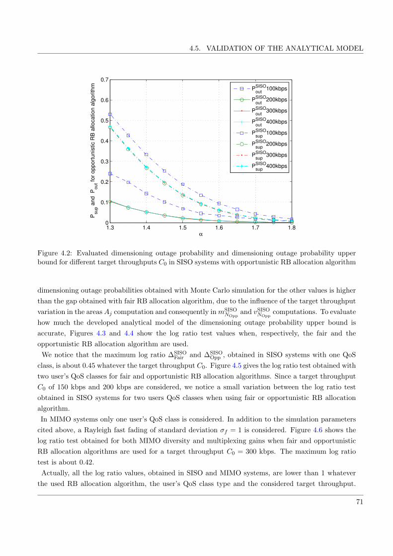
4.5. VALIDATION OF THE ANALYTICAL MODEL
1.3 1.4 1.5 1.6 1.7 1.80
0.1
0.2
0.3
0.4
0.5
0.6
0.7
α
Psup a
nd P
out f
or
opport
unis
tic R
B a
llocation a
lgorith
m
Pout
SISO100kbps
Pout
SISO200kbps
Pout
SISO300kbps
Pout
SISO400kbps
Psup
SISO100kbps
Psup
SISO200kbps
Psup
SISO300kbps
Psup
SISO400kbps
Figure 4.2: Evaluated dimensioning outage probability and dimensioning outage probability upperbound for different target throughputs C0 in SISO systems with opportunistic RB allocation algorithm
dimensioning outage probabilities obtained with Monte Carlo simulation for the other values is higher
than the gap obtained with fair RB allocation algorithm, due to the influence of the target throughput
variation in the areas Aj computation and consequently inmSISONOpp
and vSISONOpp
computations. To evaluate
how much the developed analytical model of the dimensioning outage probability upper bound is
accurate, Figures 4.3 and 4.4 show the log ratio test values when, respectively, the fair and the
opportunistic RB allocation algorithm are used.
We notice that the maximum log ratio ∆SISOFair and ∆SISO
Opp , obtained in SISO systems with one QoS
class, is about 0.45 whatever the target throughput C0. Figure 4.5 gives the log ratio test obtained with
two user’s QoS classes for fair and opportunistic RB allocation algorithms. Since a target throughput
C0 of 150 kbps and 200 kbps are considered, we notice a small variation between the log ratio test
obtained in SISO systems for two users QoS classes when using fair or opportunistic RB allocation
algorithm.
In MIMO systems only one user’s QoS class is considered. In addition to the simulation parameters
cited above, a Rayleigh fast fading of standard deviation σf = 1 is considered. Figure 4.6 shows the
log ratio test obtained for both MIMO diversity and multiplexing gains when fair and opportunistic
RB allocation algorithms are used for a target throughput C0 = 300 kbps. The maximum log ratio
test is about 0.42.
Actually, all the log ratio values, obtained in SISO and MIMO systems, are lower than 1 whatever
the used RB allocation algorithm, the user’s QoS class type and the considered target throughput.
71
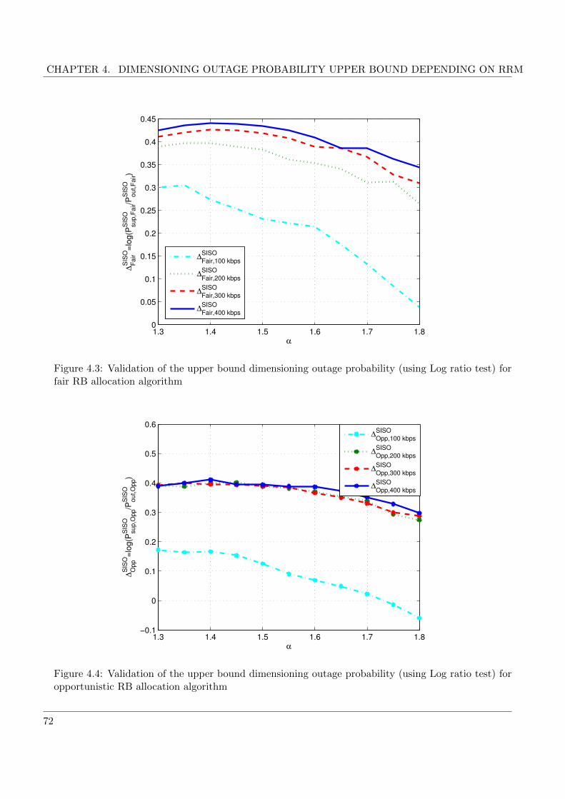
CHAPTER 4. DIMENSIONING OUTAGE PROBABILITY UPPER BOUND DEPENDING ON RRM
1.3 1.4 1.5 1.6 1.7 1.80
0.05
0.1
0.15
0.2
0.25
0.3
0.35
0.4
0.45
α
∆F
air
SIS
O=
log(P
sup,F
air
SIS
O/P
out,F
air
SIS
O)
∆Fair,100 kbps
SISO
∆Fair,200 kbps
SISO
∆Fair,300 kbps
SISO
∆Fair,400 kbps
SISO
Figure 4.3: Validation of the upper bound dimensioning outage probability (using Log ratio test) forfair RB allocation algorithm
1.3 1.4 1.5 1.6 1.7 1.8−0.1
0
0.1
0.2
0.3
0.4
0.5
0.6
α
∆O
pp
SIS
O=
log(P
sup,O
pp
SIS
O/P
out,O
pp
SIS
O)
∆
Opp,100 kbps
SISO
∆Opp,200 kbps
SISO
∆Opp,300 kbps
SISO
∆Opp,400 kbps
SISO
Figure 4.4: Validation of the upper bound dimensioning outage probability (using Log ratio test) foropportunistic RB allocation algorithm
72

4.5. VALIDATION OF THE ANALYTICAL MODEL
1.3 1.4 1.5 1.6 1.7 1.80.4
0.41
0.42
0.43
0.44
0.45
0.46
0.47
0.48
0.49
α
Log r
atio for
SIS
O w
ith 2
QoS
cla
sses
∆Fair,2QC
SISO
∆Opp,2QC
SISO
Figure 4.5: Validation of the upper bound dimensioning outage probability (using Log ratio test) forfair and opportunistic RB allocation algorithms with two QoS classes
Therefore, they validate the proposed analytical model of the dimensioning outage probability upper
bound, in SISO and MIMO systems, independently of the user’s QoS type, the target throughput and
the RB allocation algorithm.
73

CHAPTER 4. DIMENSIONING OUTAGE PROBABILITY UPPER BOUND DEPENDING ON RRM
1.3 1.4 1.5 1.6 1.7 1.80.26
0.28
0.3
0.32
0.34
0.36
0.38
0.4
0.42
0.44
c
Log r
atio test
∆Opp
Div,MIMO
∆Fair
Mux,MIMO
∆Opp
Mux,MIMO
∆Fair
Div,MIMO
Figure 4.6: Validation of the upper bound dimensioning outage probability (using Log ratio test) inMIMO systems
4.5.2 Bandwidth allocation
The adequate bandwidth B that can be allocated to a cell is then determined using the average number
of RBs and the computed dimensioning outage probability upper bound. Figure 4.7 represents the
average number of RBs needed by the network as a function of the target throughput C0, when the
fair and opportunistic RB allocation algorithm are used in SISO system for a single user’s QoS class.
To allocate these average numbers of required RBs values, we propose to associate the nearest LTE
standardized bandwidth, varying from 1.4 MHz and 20 MHz, that can be allocated.
Table 4.1 gives the dimensioning outage probability obtained by Monte Carlo simulations. If we
allocate these standardized LTE bandwidths, we obtain a dimensioning outage probability for the fair
RB allocation algorithm, P SISOout,Fair between 5.2 10−2 and 9.1 10−6. If we allocate 5 MHz more, the
dimensioning outage probability becomes very small and most of the RBs are not used. To address
the RB wastage problem and improve the spectrum use efficiency, we can use the smallest bandwidth
B = 1.4 MHz as a carrier aggregation component, which allows us to increase the number of RBs per
cell by only 6 RBs.
The same methodology is used for MIMO systems. Table 4.2 contains the average number of RBs
obtained with the analytical model for diversity and multiplexing gain MIMO systems using fair and
opportunistic RB allocation algorithms. To enlighten the MIMO gains, we compare our results with
1 × 1 diversity gain MIMO system (equivalent to a SISO system that considers only path loss and
the fading effect) using a fair RB allocation algorithm. Since MIMO system gains are relevant when
74
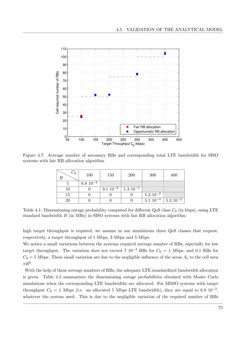
4.5. VALIDATION OF THE ANALYTICAL MODEL
50 100 150 200 250 300 350 400 4500
10
20
30
40
50
60
70
80
90
100
110
Target Throughput C0 (kbps)
Cell
required n
um
ber
of R
Bs
Fair RB allocation
Opportunistic RB allocation
Figure 4.7: Average number of necessary RBs and corresponding total LTE bandwidth for SISOsystems with fair RB allocation algorithm
HHHHHHB
C0 100 150 200 300 400
5 6.8 10−2
10 0 9.1 10−6 1.3 10−5
15 0 0 0 5.3 10−2
20 0 0 0 5.1 10−4 5.3 10−2
Table 4.1: Dimensioning outage probability computed for different QoS class C0 (in kbps), using LTEstandard bandwidth B (in MHz) in SISO systems with fair RB allocation algorithm
high target throughput is required, we assume in our simulations three QoS classes that request,
respectively, a target throughput of 1 Mbps, 3 Mbps and 5 Mbps.
We notice a small variations between the systems required average number of RBs, especially for low
target throughput. The variation does not exceed 7 10−4 RBs for C0 = 1 Mbps, and 0.1 RBs for
C0 = 5 Mbps. These small variation are due to the negligible influence of the areas Aj to the cell area
πR2.
With the help of these average numbers of RBs, the adequate LTE standardized bandwidth allocation
is given. Table 4.3 summarizes the dimensioning outage probabilities obtained with Monte Carlo
simulations when the corresponding LTE bandwidths are allocated. For MIMO systems with target
throughput C0 = 1 Mbps (i.e. an allocated 5 Mbps LTE bandwidth), they are equal to 6.8 10−2,
whatever the system used. This is due to the negligible variation of the required number of RBs
75

CHAPTER 4. DIMENSIONING OUTAGE PROBABILITY UPPER BOUND DEPENDING ON RRM
XXXXXXXXXXXC0 (Mbps)mN mSISO
N,Fair mDiv,MIMON,Fair mDiv,MIMO
N,Opp mMux,MIMON,Fair mMux,MIMO
N,Opp
1 33.5109 33.5102 33.5102 33.5107 33.5102
3 56.7700 56.7500 56.7000 56.6300 56.6200
5 75.0057 75.0040 74.9800 74.9700 74.9000
Table 4.2: Required average number of RBs in MIMO systems
in Table 4.2. For C0 = 3 Mbps (i.e. an allocated bandwidth B = 10 MHz), the dimensioning
outage probability is about 1.1 10−2 for SISO and diversity gain MIMO systems, and is null for
the multiplexing gain in MIMO system, whatever the RB allocation algorithm used. For 15 MHz
bandwidth, corresponding to a target throughput C0 = 5 Mbps, the dimensioning outage probabilities
are null for all the systems. It means that the required average number of RBs is more than enough
to satisfy and serve all users.
In Table 4.4, the smallest standardized bandwidth B = 1.4 MHz is used as a component aggregation
XXXXXXXXXXXB (MHz)Pout PDiv,SISO
out,Fair PDiv,MIMOout,Fair PDiv,MIMO
out,Opp PMux,MIMOout,Fair PMux,MIMO
out,Opp
5 6.8 10−2 6.8 10−2 6.8 10−2 6.8 10−2 6.8 10−2
10 1.15 10−2 1.15 10−2 1.10 10−2 0 0
15 0 0 0 0 0
Table 4.3: Dimensioning outage probability in MIMO systems.
in case of C0 equal to 1 Mbps and 3 Mbps (when the dimensioning outage probabilities are noticeable).
This smallest component aggregation leads to a decrease of the dimensioning outage probabilities, for
example from 6.8 10−2, before the carrier aggregation, to 0.45 10−2 after the carrier aggregation,
for C0 = 1 Mbps. Actually, the carrier aggregation decreases the dimensioning outage probabilities
whatever the system used to a dimensioning outage probability lower than the one fixed by the
operators which is usually about 1%.
Since the allocated bandwidth in case of a target throughout C0 = 5 Mbps leads to a zero dimensioning
`````````````(B,CA) (MHz)Pout PDiv,SISO
out,Fair PDiv,MIMOout,Fair PDiv,MIMO
out,Opp PMux,MIMOout,Fair PMux,MIMO
out,Opp
(5,1.4) 4.5 10−3 4.5 10−3 4.5 10−3 4.5 10−3 4.5 10−3
(10,1.4) 2.4 10−3 2.4 10−3 2.4 10−3 0 0
(10,0) 0.1175 0.1175 0.1152 1.8 10−3 1.3 10−3
Table 4.4: Dimensioning outage probability computed after modifying the allocated bandwidth inMIMO systems.
outage probability, we try to decrease the allocated bandwidth by 33%, to B = 10 MHz, corresponding
to 50 available RBs. With this reduction, the dimensioning outage probability of SISO and diversity
gain MIMO systems increases to 11%, whereas the dimensioning outage probabilities of multiplexing
76

4.6. CONCLUSION
gain in MIMO systems become on the order of 0.1 %.
These results show that the use of diversity gain MIMO systems, independently of the used RB
allocation algorithm, is not sufficient relatively to SISO systems and does not increase significantly
the rate when operating in the low SINR regime. Hence, independently of the used RB allocation
algorithm, the diversity techniques do not overcome the dimensioning outage situation compared to a
classical SISO system. On the contrary, as the multiplexing techniques increase significantly the rate
that can be transmitted, and hence decrease the required number of RBs per UE, the dimensioning
outage probability decreases significantly compared to the SISO case. We finally note that, although a
pessimistic strategy was analytically adopted to estimate the average number of RBs, a significant gain
in terms of dimensioning outage probability can be numerically observed. However, this pessimistic
strategy gives an over-estimation of the dimensioning outage probability.
4.6 Conclusion
This chapter addressed the radio dimensioning problem of SISO and MIMO LTE uplink networks.
We developed an analytical model to evaluate the dimensioning outage probability upper bound and
the average number of required RBs per cell, in order to evaluate the adequate bandwidth that should
be allocated to the network. The dimensioning outage probability upper bound was evaluated as a
function of two RRM strategies: i) fair RB allocation algorithm and ii) opportunistic RB allocation
algorithm, considering a single and multiple user’s QoS classes. The developed analytical model was
based on the stochastic geometry using the Poisson point processes, which helped us to examine the
statistical network’s behavior. To evaluate how close were the analytical model of the dimensioning
outage probability upper bound and the dimensioning outage probability obtained by Monte Carlo
simulations, a log ratio test was used. Its values validated the analytical model independently of the
used system, the target throughput or the number of user’s QoS classes. The dimensioning problem was
also extended to MIMO systems. We showed that, in the low SNR regime, when using diversity MIMO
techniques, no significant gain on dimensioning outage probability was observed compared to SISO
systems. However, the multiplexing gain strategies increased significantly the rate and consequently
decreased the dimensioning outage probability.
4.A Appendices
4.A.1 Derivation of area Aj expression in SISO system with fair RB allocation
algorithm (Formulas 4.45)
We assume γj to be the SINR threshold, j being the user’s required number of RBs to achieve its
target throughput C0, with:
γj = 2C0/(jW ) − 1 for j = 1, · · · , Nmax − 1 and γ0 =∞
77

CHAPTER 4. DIMENSIONING OUTAGE PROBABILITY UPPER BOUND DEPENDING ON RRM
We define Aj the area which contains the users that require at most j RBs to satisfy their target
throughput C0. The area Aj can be determined as follows:
Aj =
∫C×R+×Z
1y‖x‖β≤PtK/ηγj ps(y)dy p(z)dz dx
=
∫C×R+×Z
prob(y‖x‖β ≤ γj
)p(z)dz dy dx (4.36)
where γj = PtKηγj
.
The probability density function of the shadowing is:
ps(y) =ξ
σsy√
2πexp
(−(10 log10 y − µs)2
2σ2s
)(4.37)
where, ξ = 10/ ln 10.
The cumulative distribution function of S is then,
FS(y) = 12 + 1
2erf(− (10 log10(y)−µs)2√
2σs
)(4.38)
It can be expressed using the Q function3 as:
FS(y) = Q(
(10 log10(y)−µs)2√2σs
)(4.39)
From Formulas 4.36 we obtain:
Aj =1
NUE
∫x∈C
prob
(y ≤ γ
‖x‖β)dx (4.40)
where, γ = PtKηγj
Then,
Aj = 1NUE
∫x∈C
Q
10 log10(γj‖x‖β )− µsσs
dx (4.41)
= 1NUE
∫x∈C
Q
(1
σs10 log10(γj)−
µsσs− β
σs10 log10(x)
)dx (4.42)
= 1NUE
∫x∈C
Q
(1
σs10 log10(
PtK
ηγj)− µs
σs− β
σs10 log10(x)
)dx (4.43)
= 1NUE
∫ 2π
θ=0
∫ R
r=0Q (αj − ζ ln(r)) rdrdθ (4.44)
3Q(x) = 12
+ 12ref( x√
2)
78

4.A. APPENDICES
with: α = 1σs
(10 log10(PtKηγj )− µs
), and ζ = β10
σs ln(10) .
Aj = 1NUE
(14 exp
(2αjζ + 2
ζ2
)erf
(−αjζ+ζ
2 ln(R)−2√(2)ζ
)+ R2
4 + R2
4 erf(αj−ζ ln(R)√
2
)+ 1
4 exp(
2αjζ + 2
ζ2
))Then, Aj can be expressed with Φ the normal cumulative distribution function4,
Aj = νρR2 exp (2/ζ + 2αj/ζ)Φ(ζ lnR− 2/ζ − αj) + ν
ρΦ(αj − ζ lnR) (4.45)
4the normal cumulative distribution function is expressed as: Φ = 12
+ 12erf( x√
2)
79

CHAPTER 4. DIMENSIONING OUTAGE PROBABILITY UPPER BOUND DEPENDING ON RRM
80

Chapter 5
Radio resource allocation scheme for
green uplink LTE networks
Parts of this chapter were published in IEEE WCNC 20131, IEEE GREENCOM 20132 and submitted
to IEEE Transactions on Vehicular Technology3
WHEN an adequate frequency bandwidth is determined and allocated to a cell, the
RRM entity aims at allocating efficiently the limited radio resources among users. In
the uplink of green LTE networks, the radio resources allocation includes two steps:
the RBs allocation and an adequate UE transmission power allocation. Each radio resource allocation
scheme is based on an utility function which translates the system satisfaction level. In this chapter,
the cell capacity maximization is considered. For this purpose, a new radio resource allocation scheme
is proposed. It is based on the Opportunistic and Efficient RB Allocation (OEA) algorithm whose
objective is to maximize the aggregate throughput while subject to the SC-FDMA constraints. An
evolution of the algorithm, named QoS based OEA, providing QoS differentiation, is also proposed. It
allocates a given maximum number of RBs to each UE according to the user’s QoS requirements. The
UE transmission power is adjusted by a channel dependent power control such that the user’s QoS
1F.Z. Kaddour, M. Pischella, P. Martins, E. Vivier and L. Mroueh, “Opportunistic and Efficient Resource BlockAllocation Algorithms for LTE Uplink Networks”, in proceedings of IEEE Wireless Communications and NetworkingConference (WCNC), Shanghai, China, Apr. 2013.
2F.Z. Kaddour, E.Vivier, M. Pischella, L. Mroueh and P. Martins, “Green Opportunistic and Efficient Resource BlockAllocation Algorithm for LTE Uplink Networks ”, in proceedings of 3rd IEEE GreenComm online conference, October,2013.
3F.Z. Kaddour, E. Vivier, L. Mroueh, M. Pischella and P. Martins, “Green Opportunistic and Efficient ResourceBlock Allocation Algorithm for LTE Uplink Networks”, submitted to IEEE Transactions on Vehicular Technology.
81

CHAPTER 5. RADIO RESOURCE ALLOCATION SCHEME FOR GREEN LTE NETWORKS
satisfies the previous throughput determined by the RB allocation step. The proposed radio resource
allocation scheme is studied in regular and random networks.
5.1 Introduction
Nowadays, in current and next generation mobile networks, the ICT are facing increasing challenges
to satisfy the quality of service required by the smart terminals enhanced functionalities. Then the
energy consumption of wireless communication networks and the relevant global CO2 emission show
continuous growth for several years. In [68], it has been emphasized that actually the information
and communication technology infrastructures consume about 3% of the world-wild energy which
causes about 2% of the world CO2 emissions. Energy costs to the mobile’s operators half of the
operating expenses [69]. Moreover, improving the energy efficiency is not only beneficial for the
global environment, but also makes commercial sense for telecommunication operators supporting
sustainable and profitable business. The energy efficiency maximization is reached by maximizing
the user’s throughput, which is enabled with an adapted RB allocation policy, and minimizing the
UE transmission power. Within the framework of radio resource allocation, a number of technical
approaches are investigated in the literature.
We focus in this thesis on the radio resource allocation on the uplink 3GPP LTE networks. The
relevance of the SC-FDMA on the uplink is that in addition to the OFDMA advantages the PAPR
can be decreased by more than 25% compared to the OFDMA technique [70]. This advantage not
only leads to the decrease of the equalizer complexity and the cost of the mobile terminal by the same
way, but also to the decrease of the UE energy consumption. As saving UE battery life becomes the
central concern of the researchers, works on this scope focus on: (i) maximizing the available energy
and (ii) minimizing the energy consumption. The available energy can be increased by (a) the battery
capacity improvement which is, unfortunately, not sufficient and is limited due to design aspects, and
(b) using the surrounding energy sources, such as kinetic, thermal, and solar energy [71].
The UE energy consumption can be minimized by first, optimizing the hardware energy consumption,
such as choosing power efficient components and applying power management like performing sleep
modes for inactive hardware [72] or the Discontinuous Reception (DRX) in idle mode [73]. The second
solution is the adjustment of the UE parameters, like the brightness display and the processor speed
for some applications.
In the radio access network, the power consumption reduction is performed by a power control applied
on the UE transmission power. However, this could lead to a low signal to interference plus noise ratio
and a low individual throughput. Therefore, the power control should take into account the required
QoS and the channel conditions that the user experiences. The radio resource allocation decision is
made in order to satisfy a system satisfaction level such as the aggregate throughput maximization.
In this case, the RB allocation algorithm is based on the channel condition metric. In addition to the
user’s QoS requirement satisfaction, the proposed strategies and algorithms for allocating RBs to UEs
and for determining the UEs transmission power should consider the SC-FDMA adjacency constraint
82

5.1. INTRODUCTION
specific to LTE release 8 network. The SC-FDMA is also characterized by the MCS robustness
constraint, as detailed in Section 2.1.4. Due to these two constraints, most RRM algorithms proposed
in the literature for the downlink cannot be directly applied to the uplink. Moreover, the packet
scheduling occurs every subframe with 1 ms duration [9]. Then, the radio resource allocation schemes
shall be simple and efficient. Consequently, the uplink radio resource allocation solution is SRB ∈ Sthat maximizes the sum of all individual UE’s throughputs Rk ∀ k = 1, · · · , NUE , with S the set of
all possible allocations (RB,UE). Then, the uplink RRM problem is expressed as:
SRB = arg maxSRB∈S
NUE∑k=1
Rk
subject to:
1. Allocating each RB exclusively to one UE,
2. Allocating adjacent RBs to each UE,
3. Using for each UE, the same MCS over all its allocated RBs,
4. Respecting the UE transmission power limitation since the sum of the UE transmission power
over its allocated RBs should not exceed Pmax.
The uplink RRM problem was extensively studied. The optimal solution is given by an exhaustive
search (e.g. the branch and bound solution for Binary Integer Programming (BIP) [10] [74]), but
at the expense of a high complexity, since this problem is N-P complex. The heuristics proposed
in [11] [12] [13] consider the contiguity constraint, but neglect the power control (by setting the UE
transmission power at its maximum), the update of the power transmission per RB, and the MCS ro-
bustness constraint. These assumptions lead to overestimate the effective final user’s throughput and
to increase the inter-cell interference and the RB wastage, which consequently decrease the spectral
efficiency and the energy efficiency. Detailed state of the art in radio resource allocation schemes is
given in Section 5.2.
In this Chapter, an efficient radio resource allocation scheme is proposed. Our algorithm named
Opportunistic and Efficient RB Allocation (OEA) algorithm, takes into account the SC-FDMA con-
straints and the update of the UE transmission power per RB as a function of the number of allocated
RBs. This update of the signal to interference plus noise ratio has the benefit of canceling the RB
wastage ratio. We suggest a variant of the proposed algorithm, named QoS based OEA, which is
adapted to the QoS differentiation. It also maximizes the aggregate throughput, but serves more
users while each served user will be allocated no more than the set of RBs required to satisfy its target
QoS. The proposed algorithms are compared to the most relevant algorithms found in literature. For
fair performance comparison, the final user throughput calculation was established using the MCS
mode. The UE transmission power allocation is determined once the RB allocation is performed. The
proposed power control depends on the user’s QoS target and the channel conditions on the set of
allocated RBs. It maintains the user’s QoS and reduces the computation complexity compared to
joint power and RB allocation algorithms.
83

CHAPTER 5. RADIO RESOURCE ALLOCATION SCHEME FOR GREEN LTE NETWORKS
The proposed radio resource allocation scheme is detailed in Section 5.3. Section 5.4 gives its compu-
tational complexity steps. Its performance analysis is established in a regular and a random network,
where the inter-cell interference level considers the average transmission power generated by each
RB allocation algorithm. These two performance analysis are given respectively in Section 5.5.1 and
Section 5.5.2.
5.2 State of the art
The radio resource management in LTE uplink systems has been addressed in many papers. Usually,
the objective of the RRM is to maximize the aggregate throughput. Radio resource allocation includes
RBs and power allocation, that can be performed: jointly or separately. The joint allocation of RBs
and UEs transmission power is more complex. It can be solved by using game theory, as proposed
in [75] for the cognitive radio, or using BIP, by transforming the radio resource allocation problem
into a linear optimization problem, as proposed in [74]. The authors consider the RB contiguity and
the transmission power minimization as constraints of the linear optimization problem.
The separate allocation of RBs and UEs transmission power is less complex compared to the joint
one. First, the UEs transmission power allocation is determined by: i) a power control adjustment
according to the target QoS and the channel’s conditions (when channel information are available on
the allocated RBs), or ii) assuming the UEs transmission power as constant (usually set at Pmax). In
this latter case, the optimal solution for RB allocation is obtained using the BIP. In [10], the branch
and bound method is used to solve the BIP. It constitutes a tree that enumerates all the feasible
solutions. To decrease the complexity, we can separate the constraints (i.e. the contiguity constraint
and the exclusivity of the RB allocation) and fix a lower bound on the objective function which leads
to neglect the solutions with low performances.
The RB allocation process must determine, for each user k, the set of allocated RBs Ak, and the
number of allocated RBs: |Ak|. The definition of |Ak| and Ak is sometimes performed separately. In
this case, |Ak| is determined before the set itself, as it is proposed by the RB grouping algorithms
in [11] [76] [77] and [78]. These algorithms constitute Resource Chunks (RC), determined by a fixed
number of RBs, and allocate them to UEs. The number of RBs per RC is established by dividing the
total number of RBs per the total number of users. The optimal method of this kind of algorithms
is proposed in [78]. The authors propose to use the Hungarian algorithm known for its optimality
and polynomial complexity. The RC allocation decision is made considering the average channel gain
experienced by the UEs over the RCs. In [77], the authors add a fairness factor parameter to the
metric computation in order to enable a fair RC allocation among UEs. The RB grouping algorithm
proposed in [11] is more opportunistic, as the RCs are allocated to UEs that have the highest metric.
In [76], the authors consider multi-class services and take the QoS parameters into account in the
metric computation, such as the guaranteed bit rate of the required QoS class and the delay. The
drawback of these algorithms is the RCs establishment, as with the multi-user diversity, fairness in
the number of allocated RBs does not ensure fairness in throughput.
84

5.2. STATE OF THE ART
JointSeparate allocation
Power control PmaxAllocation | Ak | unknown | Ak | known | Ak | unknown
[74] [75] OEA [11] [76] [77] [78] [10] [12] [11] [13]QoS based OEA
Table 5.1: Summary of the proposed RRM algorithms
When |Ak| is not determined before the RB allocation itself, the designation of the allocated RBs
can be established by a nested approach: allocating one RB (usually, the RB that maximizes the
system satisfaction level) and expanding the RB allocation from this RB [11] [12] [13]. The Frequency
Domain Packet Scheduling - Largest Metric First (FDPS-LMF), proposed in [11], first searches the
pairs (RB,UE) that maximize the metric, and allocates them to the users. If the RBs assigned to a
selected user are not adjacent, the algorithm assigns also the in-between RBs to this user. These steps
are performed until no RBs are left unallocated or all UEs are served. If some RBs remain free, the al-
gorithm finally keeps them that way. In [12], the authors propose the Recursive Maximum Expansion
(RME) algorithm. This algorithm first searches the pair (RB,UE) that maximizes the metric and then
expands the RB allocation on the two sides of the selected RB while the considered UE maximizes the
metric. These two operations are performed recursively. At the end, the remaining RBs are allocated
to the UEs that satisfy the contiguity constraint, at the possible expense of the concerned UEs indi-
vidual throughput. The Heuristic Localized Gradient Algorithm (HLGA) proposed in [13] is similar
to the FDPS-LMF algorithm except for the management of the remaining RBs which is similar to
RME algorithm. These allocation policies are based on an opportunistic criterion; nevertheless, RME,
FDPS-LMF and HLGA introduce fairness among users by considering in the objective function the
proportional fair metric studied in [79], determined for each UE by the ratio between the logarithm
of its instantaneous throughput and its average throughput.
Our proposed algorithms: OEA and QoS based OEA algorithms, allocate the UEs transmission power
and the RBs separately. The UEs transmission power is determined by a power control adjustment
given as a function of the final target throughput and the channel conditions that the users experience
over their allocated RBs. Hence, the UEs transmission power allocation is performed after the RB
allocation step. In this latter, |Ak| and Ak are performed in a nested manner, where the final number
of allocated RBs per UE is not known. The RB expansion allocation is performed under the indi-
vidual user’s throughput increase condition which allows an efficient RB allocation. Before each RB
expansion allocation, an update of the concerned user’s channel conditions is performed, which allows
an estimation of the effective user’s individual throughput if an additional RB is allocated. This step
was neglected in the radio resource management cited earlier, which led to high RB wastage ratio.
Table 5.1 summarizes the state of the art of the radio resource management in LTE networks. It
classifies the algorithms as a function of their type of radio resource allocation and the number of RBs
to be allocated to each UE. As far as we know, the algorithm we propose is the first heuristic that
combines in a separate manner the UEs transmission power and the RBs allocation, without impos-
85

CHAPTER 5. RADIO RESOURCE ALLOCATION SCHEME FOR GREEN LTE NETWORKS
ing a given number of RBs to be allocated to each UE. However, the performances of the proposed
algorithm given in this paper are compared to the one of the algorithms allocating a constant UE
transmission power Pmax and an RB allocation performed in a nested manner where |Ak| is unknown.
For fair comparison while evaluating the energy efficiency and the UE transmission power, a power
control step is added at the end of each algorithm.
5.3 Efficient radio resource allocation scheme
The radio resource management can be considered as an assignment problem where the objective is
to obtain both the optimal allocation of RBs and the optimal transmission power for each UE. Our
objective is to elaborate a low computational complexity efficient radio resource allocation scheme
where the allocation of radio resources can be performed in less than one TTI. The efficient radio
resource allocation scheme we propose allocates the RBs and the transmission power separately. Since
the control of the UE transmission power needs the knowledge of the number of allocated RBs and the
channel conditions experienced by the user, the proposed scheme allocates the RBs before the power
control (as described in Figure 5.1). The RB allocation entity is channel dependent. It is based on
the channel conditions of each UE on each RB. This information is carried by the CQI and is given
as an input of the radio resource allocation scheme. Once the RB allocation is performed, the UE
transmission power is determined using the power control based on the minimum guaranteed bit rate
that each user can reach on its allocated RBs without reducing its throughput.
UE parameters:
CQI, Req QoS
UE Radio
Resource allocation
Figure 5.1: Opportunistic and efficient radio resource allocation scheme
5.3.1 Channel dependent RB allocation
The RB allocation process is an optimization problem, where the desired solution is the mapping
between a set of users K and a set of RBs C that maximizes the target performance. Our objective
is the maximization of the aggregate throughput, defined as the sum of all individual throughputs.
Then, the RBs allocation can be formulated as:
max∑k∈K
Rk(t) (5.1)
86

5.3. EFFICIENT RADIO RESOURCE ALLOCATION SCHEME
where Rk(t) is the individual throughput of user k at TTI t, over its whole allocated RBs, and subject
to the following constraints:
1. The exclusivity of the allocated RBs:∑k∈K
wck(t) = 1 ∀c ∈ C
2. The following contiguity constraint:
∀ k ∈ K, wck(t) = 0 ∀ c ≥ j + 2 if wjk(t) = 1 and wj+1k (t) = 0
3. The MCS robustness:
Rk(t) = rk(t)|Ak| (5.2)
where, wck(t) denotes the RBs allocation for TTI t: wck(t) = 1 if the RB c is allocated to user k,
otherwise wck(t) = 0. The RBs are supposed to be sorted in the increasing order of their carrier
frequency, and rk(t) is the instantaneous rate of user k considering the MCS robustness constraint,
expressed as:
rk(t) =NRBsc NUL
symb
Tsminc∈Ak
δck(t) (5.3)
with Ts being the time slot duration equal to 0.5 ms and δck(t) being the number of bits per resource
element allocated to UE k over the RB c at TTI t, using the MCS lookup table (Table 2.1) taken
from [80] and restricted to the used MCS for a target block error rate of 10%.
Optimal RB allocation
The previous optimization problem can be reformulated as a binary linear optimization problem as it
was previously introduced in [10]:
arg maxω
(CTω
)s.t. A.ω = 1
ωj ∈ 0, 1 1 ≤ j ≤ C.NUE
(5.4)
where, ω is the vector that contains the optimal solution of allocation defined by ωj ∈ 0, 1 for
1 ≤ j ≤ C.NUE , C being the total number of feasible allocations for one UE, subject to the contiguity
constraint and using the branch and bound method. The constraint matrix A is the expansion of C to
all UEs, subject to both the exclusivity and contiguity constraints. It contains all the possible solutions
of allocation. To decrease the matrix A dimension, we can separate it into two parts: firstly enumerate
the feasible solutions considering the contiguity constraint, and secondly introduce the exclusivity of
the allocation. Therefore, the matrix A dimensions become equal to (C.NUE×(NRB+NUE)). The cost
matrix C, of dimensions (C.NUE × 1), is obtained from A; it gives the resulting individual throughput
for each user in each configuration of allocation. In the cited reference [10], the cost matrix contains the
87

CHAPTER 5. RADIO RESOURCE ALLOCATION SCHEME FOR GREEN LTE NETWORKS
Shannon capacity corresponding to each allocation, and corresponds to the theoretical upper bound
of the capacity.
For fair comparison, in our study, C is built taking into account the standardized MCS settings and
considering the MCS robustness constraint. The proposed heuristics use as a metric Mx the mean
effective SINR, experienced over the two time slots that constitute one TTI, by each user k over
each RB c: Mx(k, c) = γeff(k,c). The following subsections describe the Opportunistic and Efficient RB
Allocation and the QoS based Opportunistic and Efficient RB Allocation algorithms.
Opportunistic and Efficient RB Allocation algorithm (OEA)
The OEA algorithm allocates RBs to a user while its individual throughput is improved. It starts
by the user who has the best SINR, when Pk = Pmax ∀ k ∈ K. So, the algorithm searches the pair
(RB,UE) which maximizes the considered metric. It allocates the RB noted c to UE noted k, and
then, it applies the expansion at the two sides of c. The algorithm compares the metric values at the
adjacent RBs (left extremity and right extremity) and allocates temporarily the RB with the highest
metric to user k. As the UE total transmission power is equally shared over its allocated RBs, its
SINR changes as a function of its number of allocated RBs. Then an update of the SINR values is
performed before each RB expansion allocation according to the following expression:
γeff(k,c) = γeff
(k,c) − 10 log(|Ak|+ 1) ∀c ∈ Ak (5.5)
Using relation (5.2), the potentially new UE individual throughput is computed according to the new
effective SINR. The RB allocation is confirmed and the set Ak updated if and only if the corresponding
UE k individual throughput is improved. When the condition is no more satisfied, the algorithm
updates the sets K and C and repeats the steps cited before, by performing a new search of pair
(RB,UE). The algorithm allows the users to be allocated all the RBs that are necessary to increase
their individual throughput. It means that, the maximum number of RBs that can be allocated to
UE k: αkmax is,
αkmax = NRB (5.6)
QoS based Opportunistic and Efficient RB Allocation algorithm (QoS based OEA)
The QoS based OEA algorithm is an RB allocation algorithm based on OEA. The main difference is
that the QoS based OEA limits the maximum number of RBs allocated to each UE according to its
target QoS. Then, αkmax is computed using the following formula:
αkmax =
⌈Rtarget,krk(t)
⌉(5.7)
where Rtarget,k is the target throughput of user k.
Once the RB allocation is performed, both the channel conditions of each user over each RB of its
88
5.4. RADIO RESOURCE ALLOCATION COMPUTATIONAL COMPLEXITY
allocated set Ak and |Ak| are given to the power control entity which allocates the UE transmission
power as detailed in next subsection.
5.3.2 Channel dependent UE transmission power allocation
At this step, the UE transmission power is still considered to be set to Pmax. First, the total throughput
Rk(t) achieved by each UE k over all its allocated RBs is computed; it represent the throughput that
user k should reach even after the reduction of its power transmission: Pe,k. To respect this constraint,
the power control entity takes into account the minimum SINR level that must be ensured to maintain
the use of the same MCS, as follows:
Pe,k =Pmax
|Ak|γtg
γeff(k,min)
(5.8)
where γtg is the SINR target, expressed in dB as:
(γtg)dB = (γMCS,k)dB + (∆γ)dB (5.9)
with, γMCS,k being the minimum SINR level required for keeping unchanged the MCS, ∆γ being a
margin, and γeff(k,min) being the minimum effective SINR experienced by user k over its whole allocated
RBs:
γeff(k,min) = min
c∈Akγeff
(k,c) (5.10)
The main steps of the radio resource allocation scheme are given in Algorithm 4 and Algorithm 5.
Radio resource allocation scheme proposed, hereafter its performance analysis is presented. Next
sections compare the performances of our proposed radio resource allocation scheme with the ones
of other well known proposed algorithms for the SC-FDMA technique. The performances are given
in terms of computational complexity, aggregate throughput, RB wastage ratio, energy efficiency and
energy consumption in both regular and random networks.
5.4 Radio resource allocation computational complexity
The computational complexity evaluation of all the RB allocation algorithm entities is detailed in the
following subsections. Assuming that in the worst case, when the target throughput is very high,
the QoS based OEA algorithm set a maximum number of allocated RBs allowed to user k: αkmaxequal to NRB, the computational complexity of QoS based OEA algorithm is upper bounded by the
computational complexity of OEA algorithm. The computational complexity of the opportunistic and
RME algorithms are considered identical due to the similarity of their RB allocation policy, excepting
the used metric. However, the global complexity of the radio resource allocation algorithms should
include, in addition, the computational complexity of the power control which is evaluated first.
89

CHAPTER 5. RADIO RESOURCE ALLOCATION SCHEME FOR GREEN LTE NETWORKS
Algorithm 4 Radio resource allocation algorithm
Inputs: Matrix Mx of NUE x NRB elements of γeff(k,c).
Set of UE : K = 1, · · · , k, · · · , NUE.Set of RBs : C = 1, · · · , c, · · · , NRB.αkmax , ∆γ , γMCS
Initialization:SRB = ∅, PUE = ∅while
((C 6= ∅) and (K 6= ∅)
)do
1) find (k, c) = arg maxk∈K,c∈C
Mx, where (k, c) ∈ K × C2) assign RB c to UE k:
SRB = SRB ∪ (c, k)Ak = Ak ∪ c
3) remove the RB c from the set C:C = C\c
4) determine the individual throughput:Rk(t) = rck(t)
5) update Mx(k, C), using (5.5).6) expand to the adjacent RBs with Algorithm 5.7) remove UE k from the set K.8) determine the transmission power Pe,k using (5.8):
PUE = PUE ∪ Pe,kend whileOutputs: SRB, PUE
90

5.4. RADIO RESOURCE ALLOCATION COMPUTATIONAL COMPLEXITY
Algorithm 5 Allocation expansion to the adjacent RBs
Inputs: k, C, Mx(k, C), Ak, Rk(t), αkmax , SRB.while |Ak| < αkmax do
a) select the neighboring RB with the highest metric:if Mx(k, c− 1) >Mx(k, c+ 1) thenc′ = Ak(1)
elsec′ = Ak(|Ak|)
end ifb) assign conditionally RB c′ to UE k by temporarily including c′ into Ak.c) compute the temporary throughput Rktemp of UE k with relations (5.2) and (5.3).if Rktemp(t) > Rk(t) then
- SRB = SRB ∪ (c′, k)- Ak = Ak ∪ c′.- C = C\c′.- update Mx(k, C) using (5.5).
else- break
end ifend whileOutput: SRB, Rk(t).
5.4.1 Power control complexity evaluation
The power control entity has to first count the number of allocated RBs to each user which is performed
with at least O(NRB) operations, and then to determine the minimum effective SINR experienced by
each UE over its whole allocated RBs, with O(NRB) operations. Consequently, these two operations,
performed for NUE users, have a O(2NRBNUE) computational complexity. Then the UE transmission
power allocation process is done with O(2NRBNUE +NUE) operations.
5.4.2 Radio resource allocation scheme computational complexity
In this section, we compute and compare the computational complexity of the radio resource allocation
scheme according to the considered RB allocation algorithms: OEA, FDPS-LMF, HLGA and RME
algorithms.
Complexity of the radio resource allocation scheme based on OEA and QoS based OEA
algorithm
Step 1) of Algorithm 4 is performed after a linear search on the remaining RBs and users in sets C and
K. At the worst case, each user will be assigned only one RB. Then, the computational complexity of
the lth run of this step is upper bounded by O((NUE−l)(NRB−l)). The user’s throughput is computed
with respect to the MCS robustness (5.2) by looking for the minimum rate in the set Ak. Hence, the
computational complexity of steps 4) in Algorithm 4 and step c) in Algorithm 5 is O(NRB − l). The
91

CHAPTER 5. RADIO RESOURCE ALLOCATION SCHEME FOR GREEN LTE NETWORKS
user’s metric update (steps 5) and d)) is performed before each new RB allocation at the expense of
a computational complexity of O(NRB − l). The RBs allocation expansion must be done as long as
αkmax is not reached. This parameter αkmax depends on the QoS desired by each user and is usually
quite low for QoS based OEA. Then, at the worst case represented with OEA (αkmax = NRB), step 6)
will be run O(NRB − l) times. Both algorithms stop allocating the RBs when all the users are served
or when there is no more RB to be allocated. Therefore, l is upper bounded by min(NRB, NUE) and
the expression of the proposed algorithms OEA and QoS based OEA complexity CO is:
CO =
min(NRB ,NUE)∑l=0
[O((NUE − l).(NRB − l)) +O(NRB − l) + 2.O((NRB − l)2)
]After some mathematical derivations, and considering the power control computational complexity
(step 8 in Algorithm 4) we obtain the following complexity:
CONUE≥NRB = O(N3RB
2+
(NUE
2− 1
2
)N2RB −
NUE
2NRB
)+O (2NRBNUE +NUE)
CONUE≤NRB = O(N3UE2 + (1
2 −3.NRB
2 )N2UE
)+O
((2N2
RB − 3NRB2 )NUE
)+O (2NRBNUE +NUE)
Thus, the computational complexity of OEA and QoS based OEA is polynomial of order 3.
Complexity of the radio resource allocation scheme based on FDPS-LMF and HLGA
algorithms
FDPS-LMF and HLGA algorithms both perform a linear search on RBs and users to find the pairs
(RB,UE). This step can be done using sorted metrics values and saving the corresponding pairs
(RB,UE). The computational complexity of the metrics values sorting isO(N2RBN
2UE) in the worst case.
Using the quick sort algorithm [81], the complexity is reduced to O(NRBNUE . log(NRBNUE)). Then,
both algorithms allocate the RBs to the corresponding users considering the contiguity constraint.
The complexity for these steps is O(NUENRB − 2). The FDPS-LMF stops the RBs allocation at this
step, whereas the HLGA allocates the free remaining RBs at the expense of O((NRB − 1).(NUE − 1))
additional operations. Therefore the final complexity for the FDPS-LMF: CF , and the HLGA: CH ,
including the power control computational complexity, are respectively:
CF = O (NRBNUE . ln(NRBNUE) +NUE .(NRB − 2)) +O (2NRBNUE +NUE)
andCH = O (NRBNUE . ln(NRBNUE) +NUE .(NRB − 2) + (NUE − 1).(NRB − 1))
+O (2NRBNUE +NUE)
Thus the computational complexity of FDPS-LMF and HLGA is in O(N2 ln(N)).
92
5.4. RADIO RESOURCE ALLOCATION COMPUTATIONAL COMPLEXITY
Complexity of radio resource allocation scheme based on RME algorithm
The RME algorithm also performs the linear search of the best pair (RB,UE), with a complexity
O((NRB − l)(NUE − l)) at the lth run of the algorithm. The complexity of the RME expansion step
that recursively finds a new pair (RB,UE) is in O((NRB−1).(NUE−1)) because the updates of C and
K are not considered. The allocation is done till all users are served or there is no more remaining
free RB. The same management method for these remaining free RBs as in HLGA is used. Therefore
the computational complexity evaluation of the RME including the computational complexity of the
power control: CR, is :
CR =
min(NRB ,NUE)∑l=0
[O (2(NUE − l)(NRB − l))] +O ((NRB − 1).(NUE − 1)) +O (2NRBNUE +NUE)
which can be also expressed as follows:
CRNUE≥NRB = O(−N3
RB
3+NUEN
2RB −
2NRB
3+ (1−NUE)
)+O (2NRBNUE +NUE)
CRNUE≤NRB = O(−N3
UE
3+NRBN
2UE −
2NUE
3+ (1−NRB)
)+O (2NRBNUE +NUE)
thus the computational complexity of the RME algorithm is polynomial of order 3.
5.4.3 Comparison of the algorithms complexity
Excepting the optimal solution which is N-P hard, we notice the polynomial form of the computational
complexity of each RB allocation algorithm, and hence of the radio resource allocation scheme by the
same way. Figure 5.2 shows the required number of operations that the eNB should perform to allocate
the radio resources to the NUE users. These results are given when a bandwidth B = 10 MHz,
corresponding to NRB = 50, is allocated to the sector. When the number of users increases, the
required number of operations needed to perform the radio resource allocation increases. FDPS-LMF
and HLGA are the algorithms that require the lowest computational complexity. In lowly loaded
networks, when NUE < 2NRB, the required number of operations performed by the RME algorithm
is less than the one performed by the OEA algorithm.
The maximum required number of operations to perform the radio resource allocation, whatever the
algorithm used when NUE ≤ 200, is less than 5.105 operations. Considering an eNB’s processor
of 2 × 34 k million of instructions per second, and 32-bit RISC cores running at 622/700 MHz,
the required time of radio resource allocation is given in Table 5.2. The required time is evaluated
whatever the RB allocation algorithm for all the LTE standardized bandwidths and a medium loaded
network (NUE = 2NRB). Note that at most the required time for radio resource allocation never
exceeds 4.7 10−2 ms. This value is quite reasonable, and enlightens the feasibility of the algorithms’
implementation in practical systems.
93

CHAPTER 5. RADIO RESOURCE ALLOCATION SCHEME FOR GREEN LTE NETWORKS
XXXXXXXXXXXAlgB (MHz)
1.4 3 5 10 15 20
OEA 8.32 10−6 1.3 10−4 6.47 10−4 5.29 10−3 3.23 10−3 4.11 10−2
RME 1.05 10−5 1.64 10−4 7.64 10−4 6.17 10−3 2.08 10−2 4.7 10−2
FDPS-LMF 1.08 10−5 9.11 10−5 3.23 10−4 1.38 10−3 3.23 10−3 6.17 10−3
HLGA 1.24 10−5 1.02 10−4 3.23 10−4 1.52 10−3 3.52 10−3 6.76 10−3
Table 5.2: Time required for radio resource allocation (in milliseconds)
0 50 100 150 2000
0.5
1
1.5
2
2.5
3
3.5
4
4.5
5x 10
5
Number of users
Num
ber
of oppera
tions
OEA
RME
FDPS−LMF
HLGA
Figure 5.2: Required number of operations for radio resources allocation
94

5.5. RADIO RESOURCE ALLOCATION SCHEME PERFORMANCES EVALUATION
5.5 Radio resource allocation scheme performances evaluation
The proposed algorithm performances evaluation are given in regular and random networks. In regular
networks, we compare the proposed radio resource allocation scheme based on OEA and QoS based
OEA algorithms with: 1) the three proportional fair schedulers cited before (RME, FDPS-LMF and
HLGA) and 2) one opportunistic RB allocation algorithm that allocates the RB to the user that ex-
periences the highest SINR, with respect to the contiguity constraint. In addition to these algorithms,
a performance comparison with the optimal RB allocation algorithm based on the binary integer pro-
gramming is done in random networks. The same UE power control process is performed once the
RB allocation process is completed by each studied algorithm.
Whatever the network topology used, a 1× 3× 3 frequency reuse pattern is used. The simulation pa-
rameters are mostly taken from the LTE standards. Each sector is allocated a bandwidth B of 5 MHz,
that corresponds to NRB = 25 available RBs. The radio resource allocation scheme performances are
studied through 1000 TTI, which involves a frequency-time correlated Rayleigh fading used in the
SINR computation step. We consider one QoS class of uniformly distributed pedestrian users where
a target throughput of 600 kbps is taken into account by the QoS based OEA.
5.5.1 Performances evaluation in regular networks
A regular network composed of 19 hexagonal cells is considered. We focus on radio resource allocation
in one sector of the central cell. The inter-cell interference level IRBeNB used in the SINR computation is
averaged over Monte Carlo simulations. We compare the performances of the algorithms as a function
of the network’s load, by varying the number of users per sector from 5 to 80 UEs, which corresponds
to a number of UE per number of RBs ratio from 20% to 320%. The simulation parameters, used for
the performance evaluation in regular networks, are summarized in Table 5.3.
Figure 5.3 shows the aggregate throughput of one sector of the central cell obtained with the studied
Antenna configuration Single Input Single OutputCellular layout Hexagonal grid,19 tri-sector cells.Max/ Min UE-eNB distance 500 m/30 mFrequency reuse pattern 1× 3× 3Carrier frequency 2.6 GHzSystem bandwidth B = 5 MHz per sector ⇒ NRB = 25
Rayleigh fading type frequency-time correlated fading coefficient h(m,n)
coef corr = 0.5,UE velocity = 3 km/hSINR margin ∆γ 0.3 dBMCS setting QPSK 1/2, 2/3, 3/4
16 QAM 1/2, 2/3, 3/464 QAM 1/2, 2/3, 3/4
Table 5.3: Simulation parameters in a regular network
algorithms. The aggregate throughput increases when the load of the cell increases. The OEA aggre-
gate throughput is higher than the aggregate throughput of the proportional fair schedulers (RME,
95

CHAPTER 5. RADIO RESOURCE ALLOCATION SCHEME FOR GREEN LTE NETWORKS
0 10 20 30 40 50 60 70 803
4
5
6
7
8
9
10
11
12
13
Aggre
gate
thro
ughput (M
bps)
Number of UE
Opport
OES
RME
FDPS−LMF
HLGA
QoS based OEA
Figure 5.3: Aggregate throughput with NRB=25 in one sector of a regular network
FDPS-LMF and HLGA) and close to the opportunistic one. The aggregate throughput generated by
the QoS based OEA increases significantly to be higher than the proportional fair schedulers when
NUE ≥ NRB. At low load, the free RBs management applied by the HLGA decreases the aggregate
throughput level compared to FDPS.
When the number of UEs exceeds the number of RBs, both OEA and QoS based OEA offer good
performances compared to the RME algorithm: actually, they achieve higher aggregate throughput
with less computational complexity. Unlike RME, FDPS-LMF and HLGA algorithms are less complex
than our proposed algorithms. However, they achieve a significantly lower aggregate throughput; the
gap with OEA varies from more than 200% at low load, to 20% when NUE = NRB. It then decreases
but is still around 5% when NUE ≥ 2.NRB. Especially when a large number of RBs are allocated to
one UE, the average transmission power per RB is low, which may lead, if no precautions are taken,
to a lower SINR per RB than the minimum one required for the most robust MCS, and consequently,
to a null resulting throughput.
To enlighten the metrics update benefits, we compute the maximum RB wastage ratio of each algo-
rithm over the simulation duration, that evaluates the number of RBs allocated to users, but with a
resulting individual zero throughput. Figure 5.4 shows that OEA and QoS based OEA completely
cancel this wastage. The RB wastage ratio of the opportunistic scheduler decreases to cancel when
NUE ≥ NRB. But the RME wastes around 98% of RBs whatever NUE , due to the proportional fair
metric, which means that up to 98 RBs out of 100 are allocated to users but do not lead to any data
transmission. Considering FDPS-LMF and HLGA algorithms, the RB wastage ratio tends to 40%,
96

5.5. RADIO RESOURCE ALLOCATION SCHEME PERFORMANCES EVALUATION
0 10 20 30 40 50 60 70 800
0.1
0.2
0.3
0.4
0.5
0.6
0.7
0.8
0.9
1
Maxim
um
RB
s w
asta
ge r
atio (
%)
Number of UE
Opport
OEA
RME
FDPS−LMF
HLGA
QoS based OEA
Figure 5.4: Maximum RBs wastage ratio in a regular network
as they compensate the proportional fair metric by their allocation policy. In addition to the high
aggregate throughput and the cancellation of RB wastage, the OEA efficiency resides in the number of
served users. Actually, the user throughput improvement constraint associated to the MCS robustness
limits the number of RBs allocated to each user, hence giving a chance to other users to be served.
Figure 5.5 represents the ratio of unallocated RBs. At low load the OEA efficiently uses 10% of the
available resources. The ratio of unallocated RBs decreases and is cancelled when NUE increases,
under appropriate user radio conditions.
Figure 5.6 and 5.7 represent the energy efficiency of the transmitted data, respectively before
and after the power control. The energy efficiency, given in bits per Joule, is defined by the ratio
between the users throughput and the corresponding UE transmission power. Before the power con-
trol, all the UEs transmit at their maximum power Pmax. Since the OEA and the QoS based OEA
algorithms achieve a higher throughput, then they achieve a higher energy efficiency. They reach
respectively 3.5 106 and 2.4 106 bits/J at low load, while the RME, FDPS-LMF and HLGA do not
exceed 0.8 106 bits/J. In highly loaded networks, the energy efficiency decreases for the five algorithms
to reach 7.5 105 bits/J for the OEA algorithm and 7 105 bits/J for the QoS based OEA algorithm,
5 105 bits/J for both HLGA and FDPS-LMF algorithms and 2 105 bits/J for the RME algorithm.
Once the power control is applied, the energy efficiency curves increase when the networks load in-
creases. Actually, in case of highly loaded networks, the number of allocated RBs to each UE is
low, due to the high number of UEs, which makes the power control more efficient. The number of
bits transmitted per Joule achieves 180 Mbits and 170 Mbits for the QoS based OEA and the OEA
97

CHAPTER 5. RADIO RESOURCE ALLOCATION SCHEME FOR GREEN LTE NETWORKS
5 10 15 20 25 30 35 40 450
0.1
0.2
0.3
0.4
0.5
0.6
0.7
0.8
0.9
Fre
e R
Bs r
atio
Number of UE
OEA
FDPS−LMF
QoS based OEA
Figure 5.5: Free RBs ratio in a regular network
0 10 20 30 40 50 60 70 800
0.5
1
1.5
2
2.5
3
3.5x 10
6
Number of UEs
Energ
y e
ffic
iency (
bits/J
)
HLGA
FDPS−LMF
RME
OEA
QoS based OEA
Opport
Figure 5.6: Average energy efficiency before power control in a regular network
98

5.5. RADIO RESOURCE ALLOCATION SCHEME PERFORMANCES EVALUATION
0 10 20 30 40 50 60 70 800
0.2
0.4
0.6
0.8
1
1.2
1.4
1.6
1.8
2x 10
8
Number of UEs
Energ
y e
ffic
iency (
bits/J
)
HLGA
FDPS−LMF
RME
OEA
QoS based OEA
Opport
Figure 5.7: Average energy efficiency after power control in a regular network
respectively. The curves are not smoothed as before for the power control curves, because the power
allocation depends on the minimum SINR range of the used MCS, which is not linear.
Figure 5.8 shows the average UE transmission power. The thick line corresponds to the UE maximum
transmission power set to 21 dBm. The minimum observed UE transmission power is about 17 dBm.
We notice that the RME does not decrease a lot the UE transmission power, due to the high number
of allocated RBs. The algorithms which allow a lowest UE transmission power are the HLGA, the
FDPS-LMF and the QoS based OEA. This large power reduction is explained by the number of RBs
allocated to each UE. Actually if |Ak| is low, PkTx is high and the power control according to γtg is
more efficient. In Figure 5.9, we represent the ratio of saved energy after power control. The RME
algorithm saves only from 2% to 25% of the UE transmission power, depending on the network’s load,
whereas the QoS based OEA algorithm saves from 28% to 58% of the UE transmission power, which
allows it to increase even more the UE battery life.
5.5.2 Performances evaluation in random networks
In this paragraph, the eNBs are represented by an independent homogeneous Poisson point process
ΠeNB = b1, b2, . . . of intensity λeNB on R2. The active users are located according to an indepen-
dent homogeneous Poisson point process ΠUE = u1, u2, . . . of intensity λUE > λeNB on R2. The
superposition of the two Poisson point processes represent our random network in a D×D square ge-
ographical region. Let NeNB be the number of eNBs. Each tri-sectored eNB transmits at a maximum
transmission power (PeNBmax)dBm = 43 dBm per sector. The users are assigned to a sector according
99

CHAPTER 5. RADIO RESOURCE ALLOCATION SCHEME FOR GREEN LTE NETWORKS
0 10 20 30 40 50 60 70 8017
17.5
18
18.5
19
19.5
20
20.5
21
21.5
Number of UEs
Avera
ge U
E tra
nsm
issio
n p
ow
er
(dB
m)
HLGA
FDPS−LMF
RME
OEA
QoS based OEA
Opport
Pmax
Figure 5.8: Average UE transmission power in a regular network
0 10 20 30 40 50 60 70 800
10
20
30
40
50
60
Number of UEs
Saved U
Es tra
nsm
issio
n p
ow
er
(%)
HLGA
FDPS−LMF
RME
OEA
QoS based OEA
Opport
Figure 5.9: Saved power (W) in a regular network
100

5.5. RADIO RESOURCE ALLOCATION SCHEME PERFORMANCES EVALUATION
−3 −2 −1 0 1 2 3−3
−2
−1
0
1
2
3
Distance (km)
Dis
tance (
km
)
Neighboring eNBs
Central eNB
Considered UEs
Figure 5.10: Random Network
to their downlink radio channel measurement as shown in Figure 5.10. For this purpose, each UE
measures the power received from each sector on the reference signal resource element (Reference
Signal Received Power (RSRP)) and selects the sector from which the highest power is received [30].
The RSRP for each UE u ∈ ΠUE is computed as:
RSRP = PeNBmax .GA(θu)Λu|Af |2 (5.11)
The sector we focus on for our RRM is randomly chosen. We denote by K the subset of ΠUE containing
NUE users that belong to the considered sector. We compare the performances of the algorithms as
a function of the network’s load, in lowly and highly loaded networks, by varying the Poisson point
process intensity of the users λUE . Table 5.4 summarizes the simulation parameters. As the metric
adopted for OEA algorithms requires the SINR computation, the interference level is estimated, by
the method presented in the following subsection.
ICI estimation
We consider the random network described above and focus on the computation of the ICI in one
sector. The total ICI level IceNB, suffered at each RB of the allocated bandwidth and received by the
concerned eNB s, is given by:
IceNB =
l∈ΠeNB∑l 6=s
Icl,eNB (5.12)
101

CHAPTER 5. RADIO RESOURCE ALLOCATION SCHEME FOR GREEN LTE NETWORKS
Poisson point D = 6 km,process parameters λeNB = 2.10−6 eNBs/m2 = 2 eNB/km2
λUE : 10−5 → 3.10−4 users/m2 = 300 users/km2
Frequency reuse pattern 1× 3× 3Carrier frequency 2.6 GHzSystem bandwidth B = 5 MHz per sector, NRB = 25Rayleigh fading type frequency-time correlated fading coefficient hm,n
coef corr α = 0.5, UE velocity v = 3 km/hSINR margin ∆γ 0.3 dBMCS settings QPSK 1/2, 2/3, 3/4
16 QAM 1/2, 2/3, 3/464 QAM 1/2, 2/3, 3/4
Table 5.4: Simulation Parameters in random network
PPPPPPPPRsAlg
NUE 2-5 5-10 10-15 15-20 20-25 25-30 30-35 35-40 40-45 > 45
RsOEA 46% 20% 8.9% 6% 4.6% 3% 3% 2.7% 2.3% 2%RsQoS 100% 100% 83% 58% 45% 37% 31% 26% 23% 21%RsOptim 46.4% 19% 8.6% 5.9% 4.5% 3.7% 3% 2.7% 1% 1%RsOpport 70% 63% 48% 46% 39% 32% 29% 24% 20% 18%RsRME 70% 63% 48% 46% 39% 32% 29% 24% 20% 18%RsFDPS 96% 93% 87% 74% 61% 54% 45% 38% 33% 30%RsHLGA 96% 93% 87% 74% 61% 54% 45% 38% 33% 30%
Table 5.5: Ratio of served UEs obtained by each algorithm as a function of NUE
where l belongs to the set of interfering sectors with the concerned eNB s.
Assuming that the random variables Icl,eNB follow the same law and are independent and identically
distributed, the central limit theorem can be invoked and the ICI level modeled as a Gaussian random
process. Since, in uplink, the total UE transmission power is equally shared over the whole allocated
RBs, then Icl,eNB depends on the average transmission power per RB: PRB, as determined by the
following formula:
Icl,eNB = PRBAlg .Λl,eNB.|h|2 (5.13)
The average transmission power per RB: PRBAlg , depends on the considered RB allocation algorithm.
Then, the average transmission power per RB is defined as:
PRBAlg = Pmax.RsAlg .NUE
NRB(5.14)
with RsAlg the average ratio of served UEs obtained by each studied RB allocation algorithm. To
ensure a correct evaluation of the ICI level and by the way a correct computation of RsAlg , we simulate
the different algorithms included in our study in a noise limited network, when no power control is
activated. Assuming NRB = 25, we obtain the values for RsAlg that are summarized in Table 5.5, as
a function of NUE .
The average UE transmission power per RB being estimated, Monte Carlo simulations determine for
102

5.5. RADIO RESOURCE ALLOCATION SCHEME PERFORMANCES EVALUATION
each realization of the UE Poisson point process of intensity λUE :
1. The ICI cdf corresponding to each RB allocation algorithm, as illustrated in Figure 5.11 for
λUE = 2.10−5.
2. The ICI CDF parameters as a function of λUE , as listed in Table 5.6. Actually, the ICI
distribution follows a Gaussian distribution with mean µ and standard deviation σ.
−115 −110 −105 −100 −95 −90 −85 −80 −75 −700
0.1
0.2
0.3
0.4
0.5
0.6
0.7
0.8
0.9
1
Inter−Cell Interference (ICI) in dB
Cum
ulativeDistributionFun
ctionof
ICI
FDPS−LMFHLGARMEOpportunisticOptimalOEAQoS basedOEA
−105 −100 −95 −90
0.01
0.02
0.03
0.04
0.05
0.06
0.07
0.08
0.09
0.1
0.11
Figure 5.11: CDF of ICI suffered on one RB, generated by each algorithm for λUE = 2.10−5 in arandom network
From Figure 5.11, we notice the impact of the RB allocation algorithm on the ICI level distribution.
We can classify the seven algorithms in three classes according to their generated ICI level. The
first class consists of OEA and the optimal RB allocation algorithm as they have almost the same
generated ICI level and the lowest one. The RME and the opportunistic algorithms form the second
class, they generate about 5 dB more of ICI than the first class. Finally, QoS based OEA, HLGA
and FDPS-LMF algorithms generate the most important ICI level, due to the number of RBs that
are allocated to each UE. Actually, allocating a few number of RBs to one UE is reflected in a high
average power per RB and a high generated inter-cell interference IRB.
Table 5.6 summarizes the distributions parameters, obtained with Monte Carlo simulations, as a
function of the network’s load. The χ2 test shows that the ICI distribution can be estimated with a
normal distribution with a confidence interval greater that 99%. It should be noticed that the ICI is
slightly overestimated as power control is not taken into account.
103

CHAPTER 5. RADIO RESOURCE ALLOCATION SCHEME FOR GREEN LTE NETWORKS
XXXXXXλUE
Algo FDPS-LMF HLGA RME Opportunistic Optimal OEA QoS based OEAµ σ µ σ µ σ µ σ µ σ µ σ µ σ
10−5 -89.17 4.51 -89.51 4.51 -90.59 4.52 -90.59 4.52 -92.89 4.49 -92.86 4.49 -88.98 4.53
2.10−5 -86.53 4.81 -86.51 4.81 -88.18 4.79 -88.18 4.80 -92.02 4.51 -91.93 4.54 -86.34 4.89
3.10−5 -84.58 5.31 -84.58 5.30 -86.44 5.30 -86.44 5.30 -91.83 5.17 -91.66 5.17 -84.50 5.33
5.10−5 -82.61 5.48 -82.61 5.48 -84.89 5.45 84.89 5.46 -92.50 5.13 -91.96 4.94 -83.09 5.37
9.10−5 -81.05 5.52 -80.95 5.53 -83.14 5.53 –83.15 5.53 -92.42 5.48 -89.76 6.11 -82.38 5.44
2.10−4 -80.13 5.71 -79.99 5.71 -82.33 5.71 -82.34 5.71 -94.70 5.59 -91.59 5.59 -81.68 5.71
Table 5.6: Parameter of the ICI distributions generated by each RB allocation algorithm (µ and σin dB)
Performance evaluation
As in regular networks, the radio resource allocation scheme simulations in random networks are run
on MATLAB. For the optimal RB allocation algorithm the bintprog function of the optimization
toolbox is used to solve the binary integer programming [82]. This function, based on the branch and
bound algorithm, avoids the enumeration of large classes of bad solutions and only lists potentially
good solutions [83]. However, the algorithm searches for an optimal solution by solving series of linear
programming relaxation problems, in which the binary integer variables indicating each RB allocation
are replaced by fuzzy values varying in the unit interval. But the maximum number of iterations that
the linear programming relaxation entity performs to find the optimal solution is limited. Beyond
this limit, it is considered that the optimal allocation decision can not be given in one TTI, and the
allocation is not performed. We notice from our simulations that this is the case when NUE exceeds
40. Thus, we use a least-squares sense polynomial approximation of the results obtained for low values
of NUE , in order to estimate the values when the BIP RB allocation can not be performed.
Figure 5.12 shows the aggregate throughput in the considered sector, averaged on 1000 TTI sim-
ulations, as a function of λUE . For the optimal, opportunistic and OEA algorithms, the aggregate
throughput increases when the number of users in the cell increases, unlike the proportional fair al-
gorithms FDPS-LMF, HLGA and RME. Actually, the latter ones aim at maximizing the aggregate
throughput while minimizing the variation between the users throughputs. When the number of users
increases, the probability that some users experience bad radio conditions increases. In such situa-
tions, they can not even use the most robust MCS. As proportional fair algorithms serve in priority
users experiencing bad radio conditions, that leads to a decrease of the aggregate throughput. The
aggregate throughput obtained by the OEA algorithm is close to the one obtained with the optimal
algorithm in the range 10−5 ≤ λUE ≤ 3 10−5, and then they both reach 9.3 Mbps in a highly loaded
network. The aggregate throughput of the QoS based OEA algorithm is close to the opportunistic
one and they both achieve up to 9 Mbps. The target throughput for the QoS based OEA is set to
600 kbps which explains the relatively low value of the aggregate throughput in a low loaded network.
Figure 5.13 represents the ratio between the number of served users and the number of active
users in the considered sector. The total number of active users is given with the RSRP decision and
it also includes the UEs with bad radio conditions that can not reach the minimum SINR value of
104
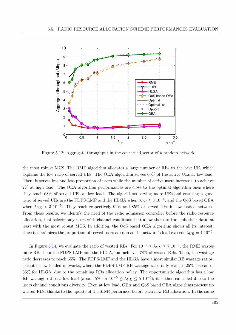
5.5. RADIO RESOURCE ALLOCATION SCHEME PERFORMANCES EVALUATION
0 0.5 1 1.5 2 2.5 3 3.5
x 10−4
0
1
2
3
4
5
6
7
8
9
10
λUE
Agg
reg
ate
th
rou
gh
pu
t (M
bp
s)
RME
FDPS
HLGA
QoS based OEA
Optimal
Optimal−es
Opport
OEA
Figure 5.12: Aggregate throughput in the concerned sector of a random network
the most robust MCS. The RME algorithm allocates a large number of RBs to the best UE, which
explains the low ratio of served UEs. The OEA algorithm serves 60% of the active UEs at low load.
Then, it serves less and less proportion of users while the number of active users increases, to achieve
7% at high load. The OEA algorithm performances are close to the optimal algorithm ones where
they reach 68% of served UEs at low load. The algorithms serving more UEs and ensuring a good
ratio of served UEs are the FDPS-LMF and the HLGA when λUE ≤ 3 10−5, and the QoS based OEA
when λUE > 3 10−5. They reach respectively 92% and 85% of served UEs in low loaded network.
From these results, we identify the need of the radio admission controller before the radio resource
allocation, that selects only users with channel conditions that allow them to transmit their data, at
least with the most robust MCS. In addition, the QoS based OEA algorithm shows all its interest,
since it maximizes the proportion of served users as soon as the network’s load exceeds λUE = 4 10−5.
In Figure 5.14, we evaluate the ratio of wasted RBs. For 10−5 ≤ λUE ≤ 7 10−5, the RME wastes
more RBs than the FDPS-LMF and the HLGA, and achieves 78% of wasted RBs. Then, the wastage
ratio decreases to reach 65%. The FDPS-LMF and the HLGA have almost similar RB wastage ratios,
except in low loaded networks, where the FDPS-LMF RB wastage ratio only reaches 25% instead of
35% for HLGA, due to the remaining RBs allocation policy. The opportunistic algorithm has a low
RB wastage ratio at low load (about 5% for 10−5 ≤ λUE ≤ 5 10−5); it is then cancelled due to the
users channel conditions diversity. Even at low load, OEA and QoS based OEA algorithms present no
wasted RBs, thanks to the update of the SINR performed before each new RB allocation. In the same
105

CHAPTER 5. RADIO RESOURCE ALLOCATION SCHEME FOR GREEN LTE NETWORKS
0 0.5 1 1.5 2 2.5 3 3.5
x 10−4
0
0.1
0.2
0.3
0.4
0.5
0.6
0.7
0.8
0.9
1
λUE
Avera
ge p
roport
ion o
f serv
ed U
E
RME
FDPS
HLGA
QoS based OEA
Optimal
Optimal−es
Opport
OEA
Figure 5.13: Average proportion of served UEs in a random network
way, the optimal algorithm cancels the RB wastage ratio whatever the intensity of users in the network.
The served users achieving an individual zero throughput are considered as unsatisfied users. Then
the behavior of the ratio of unsatisfied users is similar to the ratio of wasted RBs. The fairness criteria,
in terms of throughput, is given as a function of the users intensity per area unit in Figure 5.15. It
measures the variation of the individual throughput between satisfied users, as defined in [14] and is
expressed as:
FAlg =
(∑NUEk=1 Rk(∆T )
)2(NUE
∑NUEk=1 Rk(∆T )2
) (5.15)
We consider a short term fairness criteria, where ∆T is equal to 1 ms. The higher FAlg is, the more the
algorithm is fair. In Figure 5.15, we notice that the least fair algorithms are the opportunistic, OEA
and optimal algorithms. As we consider one class of QoS users with a target throughput of 600 kbps,
the QoS based OEA algorithm is more fair than the OEA algorithm. However, FDPS-LMF, HLGA
and RME algorithms are the most fair algorithms, due to the use of the proportional fair metric. It
must be noticed that their high number of unsatisfied users, with zero throughput, improves also their
fairness sensation.
At low load, the algorithms that allocate a low number of RBs per user without RB wastage let
more free RBs. In Figure 5.16, we represent the ratio of unused RBs. We note that the RME and
106

5.5. RADIO RESOURCE ALLOCATION SCHEME PERFORMANCES EVALUATION
0 0.5 1 1.5 2 2.5 3 3.5
x 10−4
0
0.1
0.2
0.3
0.4
0.5
0.6
0.7
0.8
0.9
λUE
Avera
ge r
atio o
f w
aste
d R
Bs
RME
FDPS
HLGA
QoS based OEA
Optimal
optimal−es
Opport
OEA
Figure 5.14: Average ratio of wastage RBs in a random network
the HLGA use NRB RBs by allocating at the end of their allocation algorithm the remaining RBs
to the users satisfying the contiguity constraints. The FDPS-LMF lets up to 24% of RBs free at low
load. Whatever the network’s load, the maximum ratio of unused RBs is achieved by the QoS based
OEA algorithm. These free RBs could be used in a cooperative network to mitigate the interference
generated by highly interfering UEs.
The average energy efficiency obtained by the different algorithms when all the UEs transmit at
Pmax is presented in Figure 5.17. Whatever the RB allocation algorithm used, the obtained average
energy efficiency curves decrease when the intensity of users per area unit increases. The algorithm
that maximizes the average energy efficiency is the optimal one. The OEA and QoS based OEA
algorithms have almost the same behavior and the obtained average energy efficiency is close to the
one obtained by the optimal algorithm. The FDPS-LMF and the HLGA algorithms achieve a lower
energy efficiency. At λUE = 3.5 10−3, the HLGA algorithm obtains a lower average energy efficiency
than the FDPS-LMF algorithm, due to the lower reached throughput caused by the allocation of the
remaining RBs. The algorithms that achieve the lowest average energy efficiency are the opportunistic
and the RME algorithms. After the power control we proposed, the behavior of the average energy
efficiency curves changes. We notice from Figure 5.18 that: i) the curves are not smoothed as before
for the power control, which is due to the nonlinearity of the throughput computation (i.e. the use of
the MCS table for the throughput computation), and ii) the average energy efficiency tends to increase
when the intensity of users per area unit increases due to the power allocation efficiency when the
number of allocated RBs to each user is low. The maximum average energy efficiency is achieved by
107

CHAPTER 5. RADIO RESOURCE ALLOCATION SCHEME FOR GREEN LTE NETWORKS
0 1 2 3 4
x 10−4
0
0.1
0.2
0.3
0.4
0.5
0.6
0.7
0.8
0.9
1
λUE
Fairness in term
of T
hro
ughput
RME
FDPS
HLGA
QoS based OEA
Optimal
Optimal−est
Opport
OEA
Figure 5.15: Fairness among users in terms of throughput in a random network
0 0.5 1 1.5 2 2.5 3 3.5
x 10−4
0
0.05
0.1
0.15
0.2
0.25
0.3
0.35
0.4
0.45
0.5
λUE
Avera
ge r
atio o
f unused R
Bs
RME
FDPS−LMF
HLGA
QoS based OEA
Optimal
optimal−es
Opport
OEA
Figure 5.16: Average ratio of unused RBs in a random network
the QoS based OEA algorithm and it reaches 1012 bits/J. Finally, the average UE transmission power
108

5.5. RADIO RESOURCE ALLOCATION SCHEME PERFORMANCES EVALUATION
0 0.5 1 1.5 2 2.5 3 3.5
x 10−4
104
105
106
107
λUE
Energ
y e
ffic
iency (
bits/J
)
OEA
QoS based OEA
Opportunistic
Optimal
Optimal−es
RME
FDPS−LMF
HLGA
Figure 5.17: Energy efficiency of the UEs in a random network, before the power allocation
0 0.5 1 1.5 2 2.5 3 3.5
x 10−4
104
106
108
1010
1012
λUE
Energ
y e
ffic
iency (
bits/J
)
OEA
QoS based OEA
Opportunistic
Optimal
RME
FDPS−LMF
HLGA
Figure 5.18: Energy efficiency of the UEs in a random network, after the power allocation
109

CHAPTER 5. RADIO RESOURCE ALLOCATION SCHEME FOR GREEN LTE NETWORKS
0 0.5 1 1.5 2 2.5 3 3.5
x 10−4
12
13
14
15
16
17
18
19
20
21
λUE
UE
s tra
nsm
issio
n p
ow
er
(dB
m)
Pmax
QoS based OEA
OEA
Opportunistic
Optimal
Optimal−es
RME
HLGA
FDPS−LMF
Figure 5.19: Average UEs transmission power in one TTI, in a random network
after power control is given in Figure 5.19. It varies between 12 dBm and Pmax = 21 dBm, and is
compliant with the standards [9]. The algorithms that allocate the highest average UE transmission
power are the RME and the Opportunistic algorithms, because they allocate the highest number
of RBs per UE. It must be noticed that the maximum transmission power of the unsatisfied users
increases the average transmission power obtained by each algorithm. As expected from the average
energy efficiency results, the algorithms that allocate the lowest average UE transmission power are
the OEA and QoS based OEA algorithms. In low loaded networks, the average saved transmission
power is about 50% when OEA, QoS based OEA, FDPS-LMF or the optimal algorithms are used.
On the contrary, the opportunistic and the RME algorithms save less than 5% of consumed power. In
highly loaded networks, the average rate of saved UE transmission power increases whatever the radio
resource allocation algorithm. It reaches around 10% for the opportunistic and the RME algorithms,
when it achieves more than 80% when the OEA and the QoS based OEA algorithms are adopted.
5.6 OEA based radio resource allocation algorithm for LTE-A net-
works
Since the OEA and QoS based OEA algorithms consider the contiguity constraint imposed in LTE
release 8 uplink air interface, they can not be directly used in LTE-A networks. To overcome this
limitation, we adapt them to the LTE-A uplink air interface, which only imposes the MCS robustness
constraint. Hence, the LTE-A adapted version of OEA algorithm steps are summarized in Algo-
110

5.6. OEA BASED RADIO RESOURCE ALLOCATION ALGORITHM FOR LTE-A NETWORKS
0 0.5 1 1.5 2 2.5 3 3.5
x 10−4
0
5
10
15
20
25
30
35
λUE
Agg
reg
ate
th
rou
gh
pu
t (M
bp
s)
OEA
QoS based OEA
OEA LTE−A
QoS based OEA LTE−A
Figure 5.20: Aggregate throughput in a concerned sector of a random LTE and LTE-A networks
rithm 6. These adapted algorithms are compared with their classical versions in terms of aggregate
throughput. The comparison is given on Figure 5.20 over 1000 TTI for a random network, where the
same simulation parameters as those cited in Table 5.4 are considered.
At low load, the aggregate throughputs are almost similar, with a small advantage for the OEA algo-
rithm and its adapted version for LTE-A networks. When the number of users increases, the aggregate
throughput increases, independently of the radio resource algorithm. Once λUE exceeds 0.3 10−4, the
aggregate throughput noticeably increases in LTE-A networks, as it achieves more than 30 Mbps,
where it does not exceed 10 Mbps in LTE. The same observation is given for the QoS differenti-
ation algorithms. The QoS based OEA adapted for LTE-A networks achieves 20 Mbps in highly
loaded networks when it converges to the one obtained with OEA algorithm in LTE. Hence, when the
RB contiguity constraint is removed, the aggregated throughput of the sector can be tripled. This
improvement is due to the users channel diversity.
111

CHAPTER 5. RADIO RESOURCE ALLOCATION SCHEME FOR GREEN LTE NETWORKS
Algorithm 6 Radio resource allocation algorithm for LTE-A networks
Inputs: Matrix Mx of NUE x NRB elements of γeff(k,c).
Set of UE : K = 1, · · · , k, · · · , NUE.Set of RBs : C = 1, · · · , c, · · · , NRB.αkmax , ∆γ , γMCS
Initialization:SRB = ∅, PUE = ∅while
((C 6= ∅) and (K 6= ∅)
)do
1) find (k, c) = arg maxk∈K,c∈C
Mx, where (k, c) ∈ K × C2) assign RB c to UE k:
SRB = SRB ∪ (c, k)Ak = Ak ∪ c
3) remove the RB c from the set C:C = C\c
4) determine the individual throughput:Rk(t) = rck(t)
5) update Mx(k, C), using (5.5).6) extend the RB allocation of UE k.while |Ak| < αkmax do
a) find (k, c′) = arg maxk∈K,c′∈C
Mx, where (k, c′) ∈ K × Cb) assign conditionally RB c′ to UE k by temporarily including c′ into Ak.c) compute the temporary throughput Rktemp of UE k with relations (5.2) and (5.3).if Rktemp(t) > Rk(t) then
- SRB = SRB ∪ (c′, k)- Ak = Ak ∪ c′.- C = C\c′.- update Mx(k, C) using (5.5).
else- break
end ifend while7) remove UE k from the set K.8) determine the transmission power Pe,k using (5.8):
PUE = PUE ∪ Pe,kend whileOutputs: SRB, PUE
112

5.7. CONCLUSION
5.7 Conclusion
In this Chapter, a new radio resource allocation scheme for uplink LTE release 8 networks, respecting
the SC-FDMA constraints, was presented. It determines the UE transmission power after the deter-
mination of the set of RBs allocated for transmission. This scheme has the benefits of adapting the
UE transmission power as a function of the user’s channel conditions over its whole allocated RBs, and
maintaining all the individual throughputs as before the power reduction. This new radio resource
allocation scheme is declined in two opportunistic and efficient versions: 1) a definitely opportunistic
one, and 2) an adapted to QoS differentiation one. The achieved aggregate throughputs are close to
the one achieved by the optimal RB allocation algorithm. As the optimal algorithm, they cancel the
RBs wastage; but in addition, they increase each served user’s energy efficiency thanks to the power
control and the individual throughput increase constraint applied for the RB expansion allocation.
The resulting saved UE transmission power increases the UE battery life and generates less inter-cell
interference. In cooperative networks, the remaining free RBs could be allocated to the neighbor-
ing users generating a high inter-cell interference. The computational complexity and the number
of necessary operations evaluation proved the hardware implementation feasibility of the proposed
radio resource scheme and its possibility to be run in less than the scheduling frequency. To adapt
the proposed radio resource allocation scheme for LTE-A networks, the RB contiguity constraint was
removed from the RB allocation algorithm. By this way, we proved that with a small modification of
the algorithm we can adapt the proposed radio resource allocation logarithm to the LTE-A networks
and maximize the network’s aggregate throughput by exploiting the user’s channel diversity.
113

CHAPTER 5. RADIO RESOURCE ALLOCATION SCHEME FOR GREEN LTE NETWORKS
114

Chapter 6
RB allocation in MU-MIMO uplink
LTE networks
Part of this chapter was published in IEEE PIMRC 20131
IN this chapter, we consider the RB allocation problem in the uplink of a multi-user MIMO
LTE network. In the MU-MIMO context, the aggregate throughput in the cell does not depend
only on the RB allocation algorithm but also on the MU-MIMO transceiver’s design. For this
reason, we focus first on the transceiver structure design and then we show how to extend the OEA
algorithm presented in Chapter 5 to the multi-user context with respect to SC-FDMA constraints.
The proposed transceiver structure is based on the use of an adequate encoder at the transmitter
side, to take advantage of the multiple transmit antenna diversity, and a combination of a joint zero
forcing (ZF) and a maximum likelihood (ML) decoder at the receiver side. The evaluated throughput
performances of the proposed transceiver in a scheduling uplink LTE context outperform the ones of
other well known decoders.
1L. Mroueh, E. Vivier, F.Z. Kaddour, M. Pischella and P. Martins, “Combined ZF and ML Decoder for UplinkScheduling in Multi-User MIMO LTE Networks ”, in proceedings of IEEE International Symposium on Personal, Indoorand Mobile Radio Communications (PIMRC), London, UK, September, 2013.
115

CHAPTER 6. RB ALLOCATION IN MU-MIMO
6.1 Introduction and Motivations
We consider Ns UEs, having nt transmit antennas each, want to communicate with an eNB having nr
receive antennas. One of the main advantages of MU-MIMO systems deployment in cellular network
is to increase the system reliability and the total data throughput in the cell. On one hand, the use
of multiple transmit antennas at both sides provides a diversity gain that can be extracted using ap-
propriate transceiver schemes. On the other hand, the use of multiple antennas at the eNB offers the
possibility to multiple UEs to transmit simultaneously on a same RB. The MU-MIMO multiplexing
over a single RB in the MU-MIMO uplink channel have been widely studied in the literature where
different scheduling strategies are proposed in [84] [85] and references therein. Most of these strategies
aim at maximizing the total aggregate throughput by choosing an appropriate combination of simul-
taneously transmitting UEs on the considered RB. However, to the best of our knowledge, few works
address the case of a MU-MIMO uplink resource allocation in the entire LTE bandwidth. Actually,
an exhaustive search (under the LTE SC-FDMA constraints) for the combination of simultaneously
transmitting UEs with maximal throughput at each RB of the LTE bandwidth becomes non feasible
when extended to several RBs. While scheduling strategies aim to offer the highest possible data
throughput, robust transceivers design aims to offer the possibility to spatially multiplex different
UEs data streams and to offer to each UE a reliable individual throughput by exploiting the transmit
and the receive diversity. Low complexity linear decoders such as ZF or Minimum Mean Square Error
(MMSE) [84] decode independently each of the transmitted data streams and lead to a loss in the
transmit diversity. The ML decoder offers both gains in diversity and multiplexing gain, but this
comes at the expense of a high decoding complexity at the eNB side [86].
This Chapter proposes a robust MU-MIMO uplink transceiver design that is based on the use of an
adequate space time code at the UE and a combination of multi-user ZF and ML decoder at the eNB.
Section 6.2 provides the MIMO an MU-MIMO background material and details the MIMO space
coding. The proposed uplink spatial multiplexing transceiver is presented in Section 6.3. The RB
allocation based on OEA algorithm in uplink MU-MIMO LTE networks is given in Section 6.4. The
performances evaluation of the proposed transceiver and the use of the OEA algorithm in MU-MIMO,
studied in a regular network, are shown in Section 6.5.
6.2 Background materials
The MU-MIMO system introduced in Section 2.3.3 is considered. In LTE systems, UEs can be
equipped by nt = 1 or nt = 2 antennas, and the eNB can have up to nr = 4 antennas. Let xk ∈ Cnt×1
denote the transmitted vector of a UE k characterized by its position (rk, θk) such that E[xkx†k] = Int .
Let Ns be the number of simultaneously active UEs in each RB. At the eNB, the received signal vector
yeNB ∈ Cnr×1 depends on the wireless channel variations and is given by,
yeNB =
K∑n=1
√PmkTxΛk Hkxk + z + I, (6.1)
116

6.2. BACKGROUND MATERIALS
where the channel matrix Hk ∈ C[nr×nt] contains the fading coefficients h(k)i,j between the antenna j of
UE k and the antenna i of the eNB, z ∈ Cnr×1 is the additive noise vector and I ∈ Cnr×1 represents
the intercell interference coming from 18 UEs in the neighboring interfering cells.
In the following, we consider the statistical inter-cell interference Iinter received at the eNB. We denote
by Σ =(N0 + Iinter
)I4 the covariance matrix of the noise plus inter-cell interference vector received
by the eNB. In addition, we note T the number of time slots over which an elementary information
signal is transmitted.
We first recall some basis on the MIMO space coding in order to fully exploit the spatial diversity and
multiplexing gains. Two different configurations are considered: the 2× 1 MISO system and the 2× 2
MIMO system. Then, in the multi-user context, we review the multi-user linear ZF decoder used to
cancel the multi-user interference.
6.2.1 Preliminaries on MIMO coding
We consider a MIMO system as depicted in Figure 6.1.
Let H[nr×nt] be the nr × nt channel matrix and let X ∈ Cnt×T be the transmitted space time code
channel
Space Time BlockCoding
ML decoder DemodulationModulation
Figure 6.1: MIMO system: Space Time coding at the encoder and Maximum Likelihood at the decoder
matrix that belongs to a codebook Xp such that
Tr[E[XX†]
]= T.
The received signal is,
Y[nr×T ] =
√PmkTxΛk
ntH
[nr×nt]k X
[nt×T ]k + (z[nr×T ] + i[nr×T ]).
where Λk is the attenuation factor induced by the path loss, the shadowing and the antenna gains,
(z + i) is the additive noise plus interference vector with covariance matrix Σ. One of the main
characteristics of MIMO systems is that one can multiplex min(nt, nr) different symbols during one
channel use. The space time code structure contains then s different symbols with s = min(nt, nr)T .
Moreover, the different symbols can be conveyed from the transmitter side to the receiver side using
ntnr different paths which correspond to the diversity gain. The space time coding scheme should
ensure that the min(nt, nr) information symbols are coded onto the different antennas in such a way
that each information symbol is transmitted through the ntnr different paths. At the receiver side,
117

CHAPTER 6. RB ALLOCATION IN MU-MIMO
the informations are decoded using a ML decoder that searches the matrix X in the family of space
time codes that minimizes the following distance,
X = arg minC∈Xp
Tr[(Y −Σ−1/2HC)(Y −Σ−1/2HC)†]
Exhaustive research among all the possible space time codewords can be performed. Algorithm with
less complexity such as sphere decoder [87] and Schnorr Euchner [88] are used in practice.
Diagonal Algebraic Space Time Block (DAST) coding for 2× 1 MISO system
For a 2 × 1 MISO system, the transmission is performed over two channels use where it is assumed
that the channel remains the same. The multiplexing gain is equal to 1, meaning that one symbol
can be transmitted over one channel use. Let s1 and s2 denote the information symbols transmitted
during the two channels use. The structure of the DAST code is
X =1√5
[x0 0
0 σ(x0)
]
where x0 = α(s1 + θs2) and σ(x0) = α(s1 + θs2) with θ = 1+√
52 , θ = 1−
√5
2 , α = 1 + i − iθ and
α = 1 + i − iθ. The main characteristics of this code is that it achieves the full diversity of the
MISO code d = 2 and the full multiplexing gain of 1 as the symbol rate is equal to 1. An intuitive
interpretation on the diversity gain can be given by observing that in this DAST coding structure,
symbol s1 (respectively s2) is transmitted over the first fading path in the first channel use and on
the second fading path in the second channel use. The DAST code transforms the MISO channel into
two parallel channels for which the capacity of the channel is,
CMISO =1
2
2∑i=1
log2(1 +PmkTx
N0 + IinterΛ|hi|2) ≤ log2
(1 +
PmkTx2(N0 + Iinter)
A(|h1|2 + |h2|2
))The effective SINR required to decode information on each channel use is then,
γeff = 2CMISO − 1
which is slightly less than the SINR of an equivalent MISO channel.
Golden code for 2× 2 MIMO system
In a 2 × 2 MIMO system, the transmission is performed over two time slots where it is assumed
that the channel remains the same. The multiplexing gain is equal to 2 meaning that two symbols
can be transmitted at once over one channel use. Let s1, s2, s3 and s4 denote information symbols
118
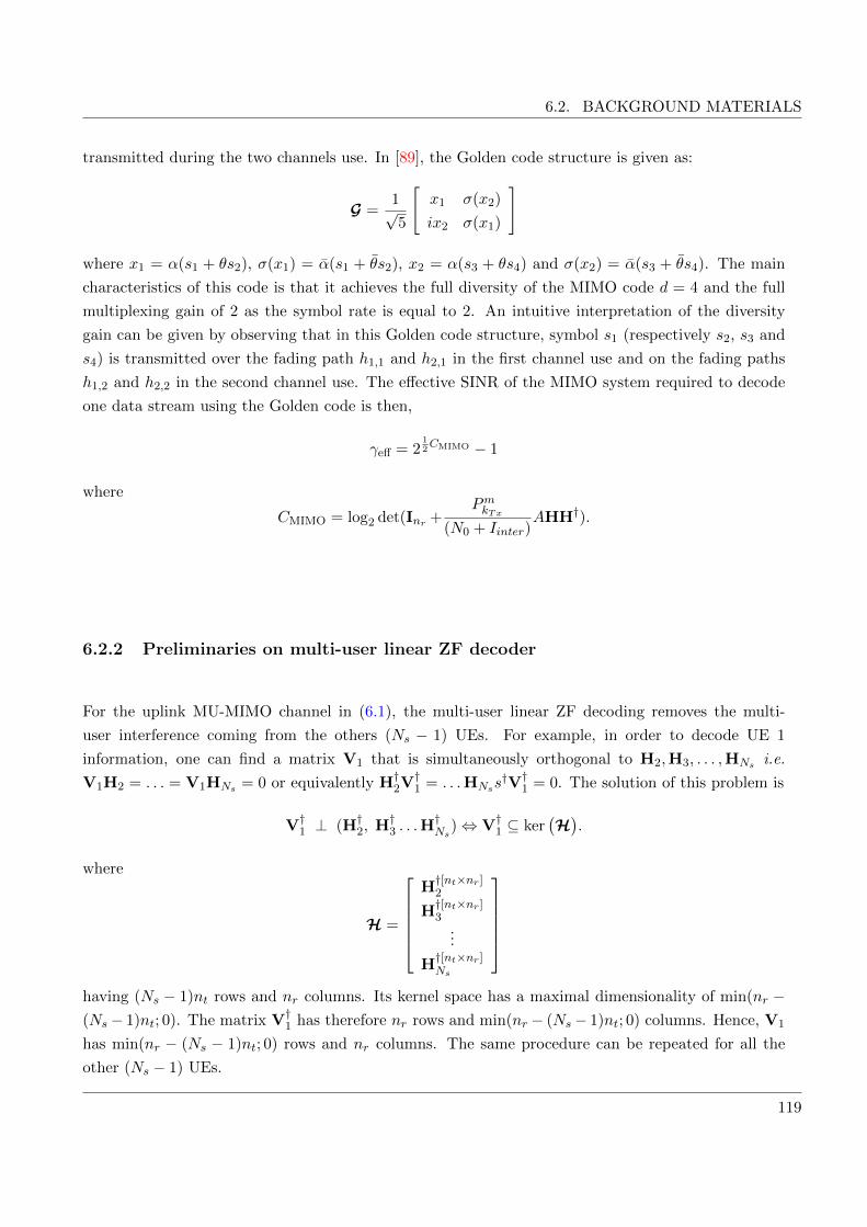
6.2. BACKGROUND MATERIALS
transmitted during the two channels use. In [89], the Golden code structure is given as:
G =1√5
[x1 σ(x2)
ix2 σ(x1)
]
where x1 = α(s1 + θs2), σ(x1) = α(s1 + θs2), x2 = α(s3 + θs4) and σ(x2) = α(s3 + θs4). The main
characteristics of this code is that it achieves the full diversity of the MIMO code d = 4 and the full
multiplexing gain of 2 as the symbol rate is equal to 2. An intuitive interpretation of the diversity
gain can be given by observing that in this Golden code structure, symbol s1 (respectively s2, s3 and
s4) is transmitted over the fading path h1,1 and h2,1 in the first channel use and on the fading paths
h1,2 and h2,2 in the second channel use. The effective SINR of the MIMO system required to decode
one data stream using the Golden code is then,
γeff = 212CMIMO − 1
where
CMIMO = log2 det(Inr +PmkTx
(N0 + Iinter)AHH†).
6.2.2 Preliminaries on multi-user linear ZF decoder
For the uplink MU-MIMO channel in (6.1), the multi-user linear ZF decoding removes the multi-
user interference coming from the others (Ns − 1) UEs. For example, in order to decode UE 1
information, one can find a matrix V1 that is simultaneously orthogonal to H2,H3, . . . ,HNs i.e.
V1H2 = . . . = V1HNs = 0 or equivalently H†2V†1 = . . .HNss
†V†1 = 0. The solution of this problem is
V†1 ⊥ (H†2, H†3 . . .H†Ns
)⇔ V†1 ⊆ ker(H).
where
H =
H†[nt×nr]2
H†[nt×nr]3
...
H†[nt×nr]Ns
having (Ns − 1)nt rows and nr columns. Its kernel space has a maximal dimensionality of min(nr −(Ns− 1)nt; 0). The matrix V†1 has therefore nr rows and min(nr − (Ns− 1)nt; 0) columns. Hence, V1
has min(nr − (Ns − 1)nt; 0) rows and nr columns. The same procedure can be repeated for all the
other (Ns − 1) UEs.
119

CHAPTER 6. RB ALLOCATION IN MU-MIMO
6.3 Uplink Spatial Multiplexing Transceiver
One of the main advantages of using MU-MIMO systems is the possibility to schedule different UEs
in the same RB using spatial division multiple access techniques. In the following, some information
theory basics from [86] [90] on the capacity region and the spatial multiplexing gain region will be first
presented. Then, we describe the proposed transceiver structure and we derive the resulting SINR
required to decode each UE’s data stream.
6.3.1 Multiplexing region of the MU-MIMO uplink channel
As mentioned in Chapter 2, the multiplexing region defines the maximal number of streams that can
be decoded simultaneously at the eNB. Over a RE, let Nu,p be the number of potential UEs among
the total number NUE of UEs, and rk with 1 ≤ k ≤ Ns be the number of streams submitted by a UE
k over a RE. Then, the multiplexing region R is defined as R =rk ∈ N : rk ≤ min(nt, nr) and rtot =∑
k rk ≤ min(nr, Nu,pnt). The min(nr, Nu,pnt) transmitted streams can be simultaneously decoded
at the eNB side using suboptimal linear decoders (such as ZF or MMSE decoder) or other optimal
decoders such as the ML decoder. Although the ML decoder improves the theoretical total throughput
compared to linear precoding schemes, this comes at the expense of an increased complexity at the
receiver side. In the following, the structure of the proposed transceiver is described.
6.3.2 Combined multi-user ZF and ML decoder
At the eNB, we propose to use a multi-user ZF decoder that only removes the multi-user interferences,
followed by a ML decoder that jointly decodes the encoded data streams. Unlike the classical ZF
decoder, the proposed combination of multi-user ZF and ML decoders can extract the multi-antenna
transmit diversity for each UE when an adequate space time code is used at the transmitter side.
The received signal in (6.1) is first equalized using a multi-user ZF decoder for each UE k in order to
.
..
...Multi User
ZF
Single User
Single User
ML
ML
.
..
yeNB
y1
yK
r1 data streams
rK data streams
Figure 6.2: Combined ZF and ML decoder: Multi-user ZF removes the multi-user interference. Thesingle-user ML decoder jointly decode the ri data streams of each user such that ri ≤ min(nt, nr) and∑K
i=1 ri = min(nr,Knt).
cancel the multi-user interference coming from the other (Ns− 1) UEs. For this purpose, the received
120

6.3. UPLINK SPATIAL MULTIPLEXING TRANSCEIVER
signal is projected in a similar way as in [91] onto the orthonormal space spanned by Vk such that:
VkHi = 0, ∀i 6= k. These orthogonality constraints consume (Ns − 1)nt degrees of freedom and the
matrix Vk, that spans the kernel space of Hconc,k formed by the concatenated matrices Hi (∀i 6= k),
has therefore min(nr − (Ns − 1)nt, 0) rows and nr columns. The structure of this decoder will be
detailed later in Subsections 6.3.3 and 6.3.4 for different MU-MIMO configurations.
6.3.3 Transceiver schemes for UEs with nt = 1
In this case, the maximal number of streams that can be transmitted by each UE k is rmax,k = 1 and
rtot = 4. This means that at most four users can transmit information simultaneously on a given RE.
Case Ns = 1
In this case, the MU-MIMO channel is equivalent to a 1× 4 SIMO system. The 4× 1 received vector
at the eNB is
y =√PmkTxΛ1h
[4×1]1 x1 + (z + i)[4×1] (6.2)
The SINR over a RE is then,
γ(m,n)1 =
PmkTxΛ1‖h1‖2N0 + Iinter
Case Ns = 2
In this case, each UE transmits only one data stream using QAM constellation symbols. The 4 × 1
received vector at the eNB is
yeNB =√PmkTxΛ1h
[4×1]1 x1 +
√PmkTxΛ2h
[4×1]2 x2 + (z + i)[4×1] (6.3)
In order to decode UE 1 information, the received signal is equalized using the precoder
V†1 ∈ C[4×3] ⊆ ker( [
h†[1×4]2
] )The projection of yeNB over V1 gives:
y3×1e,1 =
√PmkTxΛ1V
[3×4]1 y[4×1] ∈ C3×1.
The equivalent channel model for UE 1 is then,
y3×1e,1 =
√PmkTxΛ1g
[3×1]1 x1 + n
[3×1]1
with g[3×1]1 = V
[3×4]1 h
[4×1]1 a 3 × 1 Gaussian vector and n
[3×1]1 = V
[3×4]1 (z + i)[4×1] a Gaussian vector
with covariance matrix (N0 + Iinter) I3 since V1 is a unitary matrix. Using the equivalent system
model, it can be deduced that the MU-ZF decomposes the MU-MIMO into two parallel 1× 3 MISO
121

CHAPTER 6. RB ALLOCATION IN MU-MIMO
channels as shown in Figure 6.3.
Figure 6.3: The linear ZF precoder decomposes the multi-user uplink MIMO channel into two parallelSIMO 1×3 channels that do not interfere. The receive diversity is equal to 3: Virtual SIMO reception.
Case Ns = 3
The number of data streams is also limited to 1 in this case. The 4× 1 received vector at the eNB is,
yeNB =√PmkTxΛ1h
[4×1]1 x1 +
√PmkTxΛ2h
[4×1]2 x2 +
√PmkTXΛ3h
[4×1]3 x3 + (z + i)[4×1] (6.4)
In order to decode UE 1 information, the received signal is equalized using the precoder
V†1 ⊆ ker([ h
†[1×4]2
h†[1×4]3
])and V1 ∈ C2×4. The projection of yeNB over V1 gives:
y2×1e,1 =
√PmkTxΛ1V
[2×4]1 y[4×1] ∈ C2×1.
The equivalent channel model for UE 1 is then,
y2×1e,1 =
√PmkTxΛ1g
[2×1]1 x1 + n
[2×1]1
with g[2×1]1 = V
[2×4]1 h
[4×1]1 a 2× 1 Gaussian vector and n
[2×1]1 = V
[2×4]1 (z + i)[4×1] is a Gaussian vector
with covariance matrix (N0 + Iinter) I2 since V1 is a unitary matrix. Using the equivalent system
model, it can be deduced that the MU-ZF decomposes the MU-MIMO into three parallel 1× 2 MISO
channels as shown in Figure 6.4.
For UE 1, the SINR over a RE (m,n) is then,
γ(m,n)1 =
PmkTxΛ1‖g1‖2N0 + Iinter
.
122

6.3. UPLINK SPATIAL MULTIPLEXING TRANSCEIVER
Figure 6.4: The linear ZF precoder decomposes the multi-user uplink MIMO channel into three parallelSIMO 1×2 channels that do not interfere. The receive diversity is equal to 2: Virtual SIMO reception.
Case Ns = 4
The 4× 1 received vector at the eNB is then,
y =√PmkTxΛ1h
[4×1]1 x1 +
√PmkTxΛ2h
[4×1]2 x2 +
√PmkTxΛ3h
[4×1]3 x3 +
√PmkTxΛ4h
[4×1]4 x4 +(z+ i)[4×1] (6.5)
In order to decoder the information submitted by UE 1, the received signal should be projected on
the orthonormal space v1 that is simultaneously orthogonal to h2,h3 and h4. This means that:
v†1 ⊆ ker( h
†[1×4]2
h†[1×4]3
h†[1×4]4
).and implies that v1 is a 1× 4 vector. Then,
ye,1 = v[1×4]1 y[4×1] =
√PmkTxΛ1 v
[1×4]1 h
[4×1]1 x1 + v
[1×4]1 (z + i)
Let g1 = v[1×4]1 h
[4×1]1 and n1 = v
[1×4]1 (z + i)[4×1]. then,
ye,1 =√PmkTxΛ1g1x1 + n1 (6.6)
The projection of the Gaussian vector h1 onto an orthonormal vector v1 results in a complex Gaussian
variable g1. The information of a UE k (with 1 ≤ k ≤ Ns) is then decoded over each RE at the eNB
with an SINR of
γ(m,n)k = PmkTx
Λk|g1|2N0 + Iinter
.
The same procedure should be applied to decode information of UE 2, UE 3 and UE 4. Using the
equivalent system model, it can be deduced that the MU-ZF decomposes the MU-MIMO into four
parallel 1× 1 SISO channels as shown in Figure 6.5.
123

CHAPTER 6. RB ALLOCATION IN MU-MIMO
g4
g1
g2
g3
Figure 6.5: The linear ZF precoder decomposes the multi-user uplink MIMO channel into four parallelSISO 1× 1 channels that do not interfere.
6.3.4 Transmission scheme for UEs with nt = 2
In this case, the maximal number of data streams transmitted per each UE is limited to min(nt, nr) = 2,
the total number of data streams should not exceed min(nr, Nu,pnt) = 4 and Ns varies from 1 to 4 as
detailed hereafter.
Case Ns = 1
The MU-MIMO uplink channel is equivalent to a 2 × 4 MIMO channel. The two transmitted data
streams can be jointly encoded using a full diversity optimal space-time code such as the Golden
code [89]. At the eNB, each of the two UE streams is decoded over each RE with an SINR
γ(m,n)k = 2
12CMIMO − 1, (6.7)
where
CMIMO = log2
∣∣ I4 +1
nt
PmkTx(N0 + Iinter
) ΛkHkH†k
∣∣.Case Ns = 2
As for Ns = 1 case, each UE transmits two data streams that can be jointly encoded using the Golden
code to extract the full transmit diversity. At the eNB, the ZF equalizer Vk ∈ C2×4 for UE k removes
the multi-user interference and is followed by a ML decoder. The 4× 1 received signal during T = 2
slots at the eNB is then,
y[4×T ]eNB =
√PmkTx
2Λ1 H
[4×2]1 X
[2×T ]1 +
√PmkTx
2Λ2 H
[4×2]2 X
[2×T ]2 + (Z + I)[4×T ]
The decoder of UE 1 should satisfy:
V†1 ⊆ ker( [
H†[2×4]2
] )124

6.3. UPLINK SPATIAL MULTIPLEXING TRANSCEIVER
Hence V1 has dimensions 2× 4. The equivalent received signal is then,
y[2×T ]e,1 = V
[2×4]1 y[4×1] =
√PmkTx
2Λ1 G
[2×2]1 X
[2×T ]1 + n1,
where G[2×2]1 = V
[2×4]1 H
[4×2]1 . This implies that the information of UE 1 can be decoded over a 2× 2
MIMO system with full diversity and full rate coding scheme. Using the equivalent system model, it
can be deduced that the MU-ZF decomposes the MU-MIMO into two parallel 2× 2 SISO channels as
shown in Figure 6.6.
Figure 6.6: The linear ZF precoder decomposes the multi-user uplink MIMO channel into two parallelMIMO 2× 2 channels that do not interfere.
Over each RE, the SINR obtained at the eNB after MU-ZF equalization is established for each
data stream using (6.7) where
CMIMO1 = log2 det
(I2 +
PmkTxΛ1
2(N0 + Iinter)G1G
†1
).
Case Ns = 3
The first UE transmits two data streams and the two others transmit only one each. For the first UE,
the full transmit diversity can be obtained as previously via the Golden code. The two other UEs
can also benefit from the full transmit diversity by using an optimal MISO space time coding scheme
such as an Alamouti [92] or a DAST [93] code that encodes each UE’s data over two consecutive time
slots. The DAST code is more adapted as, at each time slot, it activates only one of the two transmit
antennas, at the opposite of the Alamouti code that activates both antennas. This diagonal code
structure makes the ZF equalization feasible for the three simultaneously transmitting UEs. The 4×1
125

CHAPTER 6. RB ALLOCATION IN MU-MIMO
received vector at the eNB during T = 4 time slots is,
y[4×T ]eNB =
√PmkTx
2Λ1 H
[4×2]1 X
[2×T ]1 +
√PmkTxΛ2 H
[4×2]2 X
[2×T ]2
+√PmkTxΛ3 H
[4×2]3 X
[2×T ]3 + (Z + I)[4×T ]
where X1 contains two imbricated Golden codes such that;
X1 =1√5
[a1 b1 σ(c1) σ(d1)
ιc1 ιd1 σ(a1) σ(b1)
]
X2 and X3 are DAST codes such that;
X2 =1√5
[a2 0 b2 0
0 σ(a2) 0 σ(b2)
]
and
X3 =1√5
[a3 0 b3 0
0 σ(a3) 0 σ(b3)
].
In a similar way as the previous case, the DAST code permits to turn off one antenna at each time
slot while still taking advantage of the MISO gain in term of diversity. In the first time slot, the
decoder of the UE 1 information consists first to find the kernel V1:c1 of the space composed by the
first columns of H2 and H3 which have 2 × 4 dimensions. The equivalent channel model at the first
time slot is then,
y[2×1]e,1 (1) =
√PmkTx
2Λ1G
[2×2]1 x1:c1 + n1(1)
where G1:c1 = V[2×4]1:c1 H
[4×2]1 . The kernel space of the space composed by the second columns of H2
and H3 is denoted by V[2×4]1:c2 in the following and the equivalent MIMO matrix G1:c2 = V
[2×4]1:c2 H
[4×2]1 .
The same procedure can be repeated to time slot 2, 3 and 4. This gives:
y[2×1]e,1 (1) =
√PmkTx
2Λ1G
[2×2]1:c1 x
[2×1]1:c1 + n1(1) (6.8)
y[2×1]e,1 (2) =
√PmkTx
2Λ1G
[2×2]1:c2 x
[2×1]1:c2 + n1(2) (6.9)
y[2×1]e,1 (3) =
√PmkTx
2Λ1G
[2×2]1:c1 x
[2×1]1:c3 + n1(3) (6.10)
y[2×1]e,1 (4) =
√PmkTx
2Λ1G
[2×2]1:c2 x
[2×1]1:c4 + n1(4) (6.11)
The first Golden code can be formed from slots 1 and 3 in (6.8) and (6.10), the second from (6.9)
and (6.11). This implies that the information of UE 1 can be decoded over a 2×2 MIMO system with
126

6.3. UPLINK SPATIAL MULTIPLEXING TRANSCEIVER
full diversity and full rate coding scheme. The capacity of the 2× 2 MIMO system is
C(m,n)1 =
1
2
2∑i=1
log2 det
(I2 +
PmkTxΛ1
2(N0 + Iinter)G1:ciG
†1:ci
)
The SINR over each RE required to decode each data stream is then,
γ(m,n)1 = 2
12C
(m,n)1 − 1
For UE 2 and UE 3, the decoder V2 and V3 are the same as in the previous case. By repeating
similar steps, it can be deduced that the information of UE 2 and UE 3 can be respectively decoded
on an equivalent two parallel SISO channel with diversity equal to 2 and a multiplexing gain of 1. The
capacity of this parallel channel is,
CMISO =1
2
(log2
(1 +
PmkTxΛ1
N0 + Iinter|g2(1)|2
)+ log2
(1 +
PmkTxΛ1
N0 + Iinter|g2(2)|2
)).
The SINR over the RE is,
γ(m,n)2 = 2CMISO − 1.
Using the equivalent channel model, we can deduce that the MU-ZF decomposes the channel into two
parallel MISO 2× 1 channels and one 2× 2 MIMO channel as shown in Figure 6.7.
Figure 6.7: The linear ZF precoder decomposes the multi-user uplink MIMO channel into two parallelMISO 2× 1 channels and one 2× 2 MIMO channel that do not interfere.
Case Ns = 4
Only one stream is transmitted by each UE. As in the previous case of Ns = 3, the full transmit
diversity can be also achieved here using the previously defined DAST coding scheme. The 4 × 1
127

CHAPTER 6. RB ALLOCATION IN MU-MIMO
received vector at the eNB is then,
y[4×T ]eNB =
√PmkTxΛ1 H
[4×2]1 X
[2×T ]1 +
√PmkTxΛ2 H
[4×2]2 X
[2×T ]2
+√PmkTxΛ3 H
[4×2]3 X
[2×T ]3 +
√PmkTxΛ4 H
[4×2]4 X
[2×T ]4 + (Z + I)[4×T ]
In order to decode the information submitted by UE 1, the received signal should be projected on the
orthonormal space V1 that is simultaneously orthogonal to H2,H3 and H4. This means that:
V†1 ⊆ ker( H
†[2×4]2
H†[2×4]3
H†[2×4]4
).Without DAST coding, the only possible solution is the zero matrix as the dimensionality of the kernel
space is min(4− 3× 2; 0) = 0. When using a DAST code, the received signal at the first time slot is:
y[4×1](1) =√PmkTxΛ1 H
[4×2]1
[x1
0
]+√PmkTxΛ2 H
[4×2]2
[x2
0
]
+√PmkTxΛ3 H
[4×2]3
[x3
0
]+√PmkTxΛ4 H
[4×2]4
[x4
0
]+ (Z
+I)[4×1]1:c1 (6.12)
It can be easily seen from (6.12), that the 4× 1 received signal at the eNB comes only from the first
antenna of each UE. The first column of each 4 × 2 matrix Hi, which we denote in the following by
hi:c1, contributes to the received signal. The equivalent model can be then written as:
y[4×1]1 (1) =
√PmkTxΛ1 h
[4×1]1:c1 x1 +
√PmkTxΛ2 h
[4×1]2:c1 x2
+√PmkTxΛ3 h
[4×1]3:c1 x3 +
√PmkTxΛ4 h
[4×1]4:c1 x4 + (Z + I)
[4×1]1:c1 (6.13)
The channel models in (6.13) is equivalent to the one in (6.5). The same procedure can be used to
separate UEs information. For example, to find x1 of UE 1 we need to project the received signal y
on the Kernel v[1×4]1:c1 of the space that contains the first columns of each matrix Hi with i = 2, 3, 4.
Finally, the projection of y(1) on v1:c1 gives:
ye,1(1) =√PmkTxΛ1 g1(1)x1 + n1(1) (6.14)
where g1(1) = v[1×4]1:c1 h
[4×1]1:c1 .
128

6.3. UPLINK SPATIAL MULTIPLEXING TRANSCEIVER
The received signal at the second time slot is:
y[4×1](2) =√PmkTxΛ1 H
[4×2]1
[0
σ(x1)
]+√PmkTxΛ2 H
[4×2]2
[0
σ(x2)
]
+√PmkTxΛ3 H
[4×2]3
[0
σ(x3)
]+√PmkTxΛ4 H
[4×2]4
[0
σ(x4)
]+(Z + I)
[4×1]1:c2 (6.15)
Similarly, it can be seen from (6.15), that the 4 × 1 received signal at the eNB comes only from the
second antenna of each UE. The second column of each 4 × 2 matrix Hi, which we denote in the
following by hi:c2 contributes to the received signal. The equivalent model can be then written as:
y[4×1](2) =√PmkTxΛ1 h
[4×1]1:c2 σ(x1) +
√PmkTxΛ2 h
[4×1]2:c2 σ(x2)
+√PmkTxΛ3 h
[4×1]3:c2 σ(x3) +
√PmkTxΛ4 h
[4×1]4:c2 σ(x4) + (Z + I)
[4×1]1:c2 (6.16)
Similarly, the channel model in (6.16) is equivalent to the one in (6.5). The same procedure can
be used to separate UEs information. To find σ(x1) of UE 1 we need to project the received signal y
on the Kernel v[1×4]1:c2 of the space that contains the second columns of each matrix Hi with i = 2, 3, 4.
Finally, the projection of y(2) on v1:c2 gives:
ye,1(2) =√PmkTxΛ1 g1(2)σ(x1) + n1(2) (6.17)
where g1(2) = v[1×4]1:c2 h
[4×1]1:c2 .
From (6.14) and (6.17) and using the fact that g1(1) and g1(2) are Gaussian variable such that
E[g1(1)g1(2)
]= E
[v1:c1h1:c1h
†1:c2v
†1:c2
]= 0, it can be deduced that the information of UE 1 can
be decoded over a set of two parallel independent channels, which is equivalent in term of its error
probability to a 2× 1 MISO system. The capacity of 2 parallel SISO channel is,
CMISO =1
2
(log2
(1 +
PmkTxΛ1
N0 + Iinter|g1(1)|2
)+ log2
(1 +
PmkTxΛ1
N0 + Iinter|g1(2)|2
)).
The SINR over the RE is,
γ(m,n)1 = 2CMISO − 1.
Using the equivalent channel model, we can deduce that the MU-ZF decomposes the channel into four
parallel MISO 2× 1 channels in Figure 6.8.
129

CHAPTER 6. RB ALLOCATION IN MU-MIMO
Figure 6.8: The linear ZF precoder decomposes the multi-user uplink MIMO channel into four parallelMISO 1× 2 channels that do not interfere. The transmit diversity is equal to 2: Virtual MISO.
6.4 RB Allocation in the Uplink of Multi-User MIMO LTE Net-
works
Based on the above transceiver structure, we present different strategies for multi-user allocation over
one single RB. Then, we show how it can be extended to the whole LTE bandwidth under the SC-
FDMA constraints. We note that these RB allocation strategies are independent of the transceiver.
6.4.1 Multi-user allocation strategies over one RB
As stated in Section 6.3, over each RB, a maximal number of 1 ≤ Ns ≤ 4 UEs can be selected to
simultaneously transmit. For a given RB, different strategies can be used to select these Ns UEs
among a total number Nu,p of potential UEs, as detailed in the following:
One RB random allocation
The random pairing strategy selects a maximal number Ns = min(nr, Nu,p) of randomly chosen UEs,
to simultaneously transmit, independently of the wireless channel propagation conditions.
One RB opportunistic allocation with maximal metric
All the potential UEs are sorted according to their CQI defined by their effective SINR received at the
eNB when each UE is assumed to be the only transmitting UE. The eNB scheduler selects then Ns
UEs that are adequately chosen among the best CQI UEs in order to maximize a predefined metric
(Mrate or MUE). The metric Mrate aims at maximizing the RB capacity: the scheduler chooses
among the min(nr, Nu,p) best CQI UEs, Ns ≤ min(nr, Nu,p) UEs having the maximal aggregate
throughput. The metric MUE aims at maximizing the number of simultaneously transmitting UEs
per RB: the scheduler chooses, the maximal number min(nr, Nu,p) of best CQI UEs independently of
their aggregate throughput.
130

6.4. RB ALLOCATION IN THE UPLINK OF MULTI-USER MIMO LTE NETWORKS
One RB opportunistic allocation with maximal orthogonality
All the potential UEs are also sorted here in function of their CQI. The maximal orthogonal (Orth)
strategy searches, among a predefined number of best CQI UEs, the set A of semi-orthogonal UEs.
The semi-orthogonality is defined with respect to a threshold angle between fading vectors for nt = 1
and a threshold chordal distance between the fading matrices for nt = 2 [94]. This semi-orthogonality
is studied for fading vectors or matrices corresponding to the fading coefficients on the 6th subcarrier
of the considered RB. This assumption holds since the coherence bandwidth is much larger than the
RB bandwidth and the values of the correlated frequency fading coefficients do not change signifi-
cantly within one RB from its center to its extremities. Then, the scheduler selects, for simultaneous
transmission, the Ns UEs within A, that maximize Mrate or MUE.
6.4.2 Extension to the whole LTE bandwidth
We extend here the one RB multi-user allocation strategies to the whole LTE bandwidth, with respect
to the localized SC-FDMA constraints.
Random matching scheduling (RMS) algorithm
The Random Matching Scheduling (RMS) extends the one RB random allocation strategy to the
whole LTE bandwidth. First, the number of RBs allocated per UE: NRB,u, is computed depending on
the total number NUE of UEs in the cell,
NRB,u = min(⌈nr ×NRB
NUE
⌉, 1).
Then, the RBs are allocated in the ascending order by choosing, every NRB,u RBs, Ns new randomly
selected UEs.
Central opportunistic scheduling (COS) algorithm
The Central Opportunistic Scheduling (COS) algorithm extends the one RB opportunistic allocation
to the whole LTE bandwidth. It recursively selects a central (UE, RB) pair. The first pair corresponds
to the (UE, RB) pair that maximizes the CQI over all the UEs and RBs. For this central RB, Ns
UEs are selected according to one of the pre-defined metrics. Then, the COS algorithm extends the
allocation to the adjacent RBs while the central UE remains among the Ns selected UEs. If this
condition is not satisfied, the algorithm searches for a new central (RB, UE) pair that maximizes
the CQI over all the other remaining potential UEs and the non allocated RBs. The procedure is
repeated until no more RBs or UEs are available. The main steps of this algorithm are summarized in
Algorithm 7. An individual Rate Increase (RI) condition similar to the OEA algorithm can be added
to the COS. It consists in checking that the new allocated adjacent RB increases the individual rate
of each UE. In this case, a search for a new central (RB, UE) pair will be activated as soon as the
131

CHAPTER 6. RB ALLOCATION IN MU-MIMO
Algorithm 7 Central opportunistic scheduling-COS algorithm
1: Select a first central (RB, UE) pair with a maximum CQI.2: repeat3: Select Ns UEs for this central RB according to one of the pre-defined metrics.4: while the central UE is among the Ns selected UEs on the adjacent RB do5: Extend the allocation to the adjacent RBs6: end while.7: Search for a new central (RB, UE) pair with a maximum CQI.8: until no more RBs or UEs are available.
individual throughput increase (RI) condition is not satisfied by the central UE. For the other UEs,
the scheduler allocates this RB only to the UEs satisfying this RI condition.
6.5 Performance evaluation
0
10
20
30
40
50
60
20 40 60 80 100 120 140
Ag
gre
gat
e th
rou
gh
pu
t (M
bp
s)
Number of UEs
COS: Rate + Orth + RICOS: Rate + OrthCOS: Rate + RICOS: RateCOS: UEs + Orth + RICOS: UEs + OrthCOS: UEs RMS
Figure 6.9: Aggregate throughput in the cell for RMS and COS algorithms using the combined multi-user ZF-ML decoder with nt = 1
In this section, we compare the performances of these algorithms in a regular network. Each
sector is allocated a 5 MHz bandwidth. The inter-cell interference is estimated considering a highly
loaded network where each RB of the interfering cell is shared by four simultaneously transmitting
UEs. Simulations show that iinter can be generated by a Gaussian distribution with mean value
Iinter = −124 dBW and standard deviation 0.9 dB.
132

6.5. PERFORMANCE EVALUATION
For RMS and COS algorithms using the combined ZF-ML decoder with nt = 1, Figure 6.9 and 6.10
illustrate the performances of respectively Mrate and MUE (referred as Rate and UE in the figures)
by giving respectively the aggregate throughput and the percentage of served UEs in the cell. The
impact of the additional optional constraints: Orthogonality (Orth) and/or rate increase (RI), is also
depicted.
As expected for Figure 6.9, the Mrate metric leads to higher capacity than the MUE metric.
However, the gap between MUE and Mrate set of curves can be significantly reduced when adopting
the Orth constraint and, to a lesser extent, the RI constraint. The RMS algorithm becomes rate-
limited when the number of UEs in the cell exceeds nr × NRB, as beyond this limit only one RB is
allocated to each randomly chosen UE.
Figure 6.10 shows the limit ofMUE in COS algorithms without Orth and RI constraints. Actually,
MUE selects the four best CQI UEs for the best RB. Then, as the fading coefficients are correlated
from one RB to its neighbors, it is more probable that the 4 selected UEs will remain the best CQI
UEs on a consequent number of contiguous RBs if no additional constraint is imposed. This explains
the relatively bad fairness among UEs when Orth and RI constraints are not considered. We note that
the COS algorithm which associatesMUE, Orth and RI constraints presents a good tradeoff between
fairness and aggregate throughput.
30%
40%
50%
60%
70%
80%
90%
100%
20 40 60 80 100 120 140
Per
cen
tag
e o
f se
rved
UE
s
Number of UEs
RMSCOS: UEs + Orth + RICOS: UEs + OrthCOS: UEs COS: Rate + Orth + RICOS: Rate + OrthCOS: Rate + RICOS: Rate
Figure 6.10: Percentage of served UEs in the cell for RMS and COS algorithms using the combinedmulti-user ZF-ML decoder with nt = 1
133

CHAPTER 6. RB ALLOCATION IN MU-MIMO
0
10
20
30
40
50
60
70
80
90
100
20 40 60 80 100 120 140
Ag
gre
gat
e th
rou
gh
pu
t (M
bp
s)
Number of UEs
Upper bound MLUpper bound combined ZF-MLUpper bound classical ZFSymmetric MLCombined ZF-MLClassical ZF
Figure 6.11: Comparison of the combined ZF-ML decoder, the classical ZF decoder and the symmetricML decoder for nt = 2
The rate performance of the combined ZF-ML decoder, the classical ZF decoder and the symmetric
ML are compared in Figure 6.11 for nt = 2 and usingMrate metric with Orth and RI constraints. The
upper bound of each decoder is obtained when no MCS constraint is considered, and underlines the
theoretical good performances of ML decoder towards the other decoders. In the LTE context, the
ML decoder attributes the corresponding MCS to each UE by searching for a feasible J -tuple of rate
in the uplink MU-MIMO capacity region defined in (2.15). To limit this search complexity, we assume
a symmetric ML decoder for which, at each RB, all the UEs have the same MCS. Consequently, at
each RB, the Ns selected UEs should adjust their individual throughputs to the minimal one imposed
by the capacity region.
The classical ZF decodes independently the two data streams of one single UE and attributes to this
UE the minimal MCS of both data streams. Hence, the total rate provided by this decoder, in Figure
6.11, is 40% lower than the one of combined ZF-ML.
Finally, as seen from Figure 6.9 and 6.11, a second antenna transmitter per UE increases the aggregate
throughput, but at the expense of the number of served UEs.
134

6.6. CONCLUSION
6.6 Conclusion
In this chapter, we proposed a robust transceiver for multi-user MIMO scheduling in the uplink of
LTE networks. This transceiver is based on the use of an adequate space time encoder at the UE and
a combined multi-user ZF-ML decoder at the eNB. The rate performances of this transceiver were
evaluated in a LTE context when using a proposed central opportunistic scheduling (COS) algorithm.
We showed that a tradeoff between the number of served UEs and the cell total throughput is provided
when the COS maximizes the number of orthogonal served UEs per RB, conditioned by their individual
throughput increase. Finally, as a consequence of the LTE MCS constraint, the combined ZF-ML
decoder rate outperformed the symmetric ML and classical ZF decoders rates.
135

CHAPTER 6. RB ALLOCATION IN MU-MIMO
136

Conclusion and Perspectives
THIS thesis has studied a distributed radio resource management in the uplink of green LTE
networks, aiming to allocate radio resources to users with respect to their QoS requirements
in order to maximize the networks capacity. For this purpose, a channel dependent radio
resource allocation scheme was adopted.
A new ICI estimation model adapted to the UE power control process was first elaborated to
estimate the ICI level received at a given eNB from interfering UEs located in the neighboring sectors
and that are transmitting on the same RB. We showed that the ICI level generated by a virtual UE
located at the barycenter of the active user’s interfering sector and radiating at a median power of the
UEs transmission power gives a good estimation of the statistical ICI level. This model was validated
by numerical results using the statistical log ratio and Kullback-Leibler tests, and analytically where
an analytical expression of the median and mean of the UEs transmission power was derived. Then,
we considered the radio resource dimensioning problem within one cell to determine, with respect to
its radio channel conditions, the average number of RBs required by a UE to achieve a given QoS. If
the total number of RBs in the network was not sufficient to satisfy the UE’s QoS, UE was classified
in outage. For dimensioning stress, an analytical model of the dimensioning outage probability upper
bound was proposed. This dimensioning outage probability was established according to the networks
configuration, by considering a statistical behavior of UEs and the offered QoS. An upper-bound on
the dimensioning outage probability upper bound was developed, considering the RRM strategies,
for single and multiple user’s QoS class in SISO systems and for diversity and multiplexing gain in
MIMO systems. Fair and opportunistic RB allocation algorithms were considered. A comparison with
the realistic dimensioning outage probability obtained from Monte Carlo simulations was given and
the model validation was proved using the statistical log ratio test. From these results an adequate
bandwidth was allocated to the cells. With carrier aggregation technique, a small additional LTE
bandwidth was used as a carrier component to decrease the dimensioning outage probability.
Finally, the management of the limited radio resource was investigated. We proposed a new radio
resource allocation scheme (referred as OEA in this thesis) that allocates efficiently the RBs to UEs
while minimizing the UEs power consumption. The proposed RB allocation algorithm was developed
in the context of LTE release 8 and hence it respects the SC-FDMA constraints. This algorithm
was also adapted to the uplink of LTE-A networks where the OFDMA technique is adopted. In
both cases, the achieved aggregate throughput obtained with the OEA algorithm is close to the one
137

CONCLUSION AND PERSPECTIVES
achieved by the optimal RB allocation algorithm. However, the complexity of the OEA algorithm has
low computational complexity compared to other well known RB allocation algorithms in literature.
Furthermore, this algorithm minimizes the RB wastage and increases UEs energy efficiency thanks to
the power control and the individual throughput increase constraint applied for RB expansion allo-
cation. The resulting saved UE transmission power increases the UE battery life and generates less
inter-cell interference. An extension of the radio resource allocation scheme to MU-MIMO systems
was also investigated, using a new transceiver that combined ZF and ML decoders.
The proposed methods and algorithms proposed in this thesis should be complemented by addi-
tional studies. We hereunder provide first steps insights into open issues that have not been addressed
in the thesis, and that could be studied in a future work:
• The ICI estimation model was proposed for green LTE network when a single RB is allocated
to each UE. Since in SC-FDMA technique, the UE transmission power is equally shared over
the allocated RBs, the median power of the virtual point should consider the UE average trans-
mission power per RB, by considering the number of RBs allocated to each UE, in a multiple
RB allocation case.
• In the framework of LTE networks dimensioning, the dimensioning outage probability upper
bound developed for diversity and multiplexing gain of MIMO systems, when an opportunistic
RB allocation algorithm is used, considers a pessimist policy by dimensioning over the path that
requires the highest number of RBs. For further improvement, the real UE required number of
RBs should be computed, by considering the channel condition of each antenna independently.
For this purpose, successive interference cancellation methods can be used to evaluate the UEs
required number of RBs that satisfies their QoS without wasting RBs.
• The results obtained with the OEA and QoS based OEA algorithm were close to the optimal
one. Their low computational complexity proves the LTE hardware implementation. Using these
algorithms in cooperative networks can improve the network’s coverage and manage the ICI by
allocating the unused RBs to users that are in outage in the neighboring cells or generating a
high ICI level. The complexity of applying these algorithms in cooperative networks, and the
overhead exchange between the eNBs should be evaluated.
• The study given in MU-MIMO systems should consider the power control process applied in
green LTE networks and the transceiver structure should be adapted to reduce the total con-
sumed power especially when multiple radio resources are allocated to a single UE.
138

Appendix A
Correlated fast fading
Assume h(t, τ) the time varying channel response at a Dirac impulse and H the linear operator that
describe the channel. The wireless fast fading can be characterized by two function. The first is
the delay-Doppler spreading function SH(ν, τ) defined as Fourier transform (t→ ν) of h(t, τ) , where
ν denote the Doppler spread caused by the movement of the transmitters, receivers and scatterers
generated as detailed in section A.1. The second is the time varying transfert function LH(t, f)
defined as a Fourier transform (τ → f) of h(h(t, τ)). The relatonship between these system function
is given by,
LH(t, f) =
∫τh(t, τ)e−j2πfτdτ, (A.1)
SH(ν, τ) =
∫νh(t, τ)e−j2πνtdt, (A.2)
LH(t, f) =
∫τ
∫νSH(ν, τ)ej2π(νt−τf)dνdτ. (A.3)
and is summarized in Figure A.1.
A.1 Generating a frequency correlated Rayleigh fading
This method generate only frequency correlated fast fading coefficients. Since different paths are of
different lengths, a single impulse sent from the transmitter will result in multiple copies being received
at different times.
The effects of scatterers in discrete delay ranges are grouped together into individual ”taps” with the
same delay; each tap represents a single beam. Each taps has a gain which varies in time according
139

APPENDIX A. CORRELATED FAST FADING
h(t, τ)
Ft→ν Fτ→f
SH(ν, τ) Fν→t,τ→f
LH(t, f)
Figure A.1: Relationship between the channel transfer function [1].
Page 164 of 209 !2007-2008 WiMAX Forum
V2.1 Created on July 7, 2008164WiMAX System Evaluation Methodology
!"#$%&'(%)%$*#+&,$&-.#/$0"(1"$."#$/#1#(2#*$3(45&+$6#17%#3$5#4+(4(6+#$(3$1&++#*$%&'(%)%$delay spread$τ%&'8$ $ 9$+&/4#$τ%&'$(5*(1&.#3$&$"(4"+,$!"#$%&#"'%$1"&55#+8$ $ :-.#5$/77.;%#&5;3<)&/#$=/%3>$2&+)#$7-$."#$*#+&,;3?/#&*$τ/%3$(3$)3#*$(53.#&*$7-$."#$%&'(%)%8$
!"#"$%&'(()*%+),'-%./0)%12*),%:5#$0&,$.7$/#?/#3#5.$."#$(%?)+3#$/#3?753#$7-$&$%)+.(?&."$1"&55#+$(3$6,$&$*(31/#.#$5)%6#/$7-$(%?)+3#3$&3$-7++703@$
A
= B > = > = >(
" ""
) * + *τ δ τ τ=
= −"
C7.#$."&.$."#$(%?)+3#$/#3?753#$"$2&/(#3$0(."$.(%#$.8$ $ !"#$17#--(1(#5.3$1(=.>$2&/,$0(."$.(%#8$ $ !"#/#$&/#$C$17#--(1(#5.3$(5$."#$&672#$%7*#+8$ $ !"#$3#+#1.(75$7-$."#$C$&5*$*#+&,$2&+)#3$τ($*#?#5*3$)?75$0"&.$(3$1753(*#/#*$&$3(45(-(1&5.$+#2#+8$ $ !"(3$%7*#+$/#?/#3#5.3$."#$1"&55#+$6,$&$*#+&,$+(5#$0(."$C$.&?38$ $ D7/$#'&%?+#B$."#$1"&55#+$3"705$(5$D(4)/#$98A8E$1&5$6#$/#?/#3#5.#*$6,$&$F;.&?$%7*#+$&3$3"705$(5$D(4)/#$98A8G8$
$
τ1 τ2 τ3 τ4
H#+&,I(5#$
1A1J 1K 1F
$
Figure A.1.6: Tapped Delay Line Model
L-$."#$./&53%(..#/B$/#1#(2#/B$7/$#2#5$."#$7."#/$76M#1.3$(5$."#$1"&55#+$%72#B$."#$1"&55#+$1"&/&1.#/(3.(13$1"&54#8$ $ !"#$.(%#$-7/$0"(1"$."#$1"&55#+$1"&/&1.#/(3.(13$1&5$6#$&33)%#*$.7$6#$1753.&5.$(3$1&++#*$coherence time8$!"(3$(3$&$3(%?+(3.(1$*#-(5(.(75$(5$."#$3#53#$."&.$#'&1.$%#&3)/#%#5.$7-$17"#/#51#$.(%#$/#<)(/#3$)3(54$."#$&).717//#+&.(75$-)51.(758$
D7/$#2#/,$?"#57%#575$(5$."#$.(%#$*7%&(5B$."#/#$(3$&$17//#3?75*(54$?"#57%#575$(5$."#$-/#<)#51,$*7%&(58$ $ L-$0#$+77N$&.$."#$D7)/(#/$./&53-7/%$7-$."#$?70#/$*#+&,$?/7-(+#B$0#$1&5$76.&(5$."#$-/#<)#51,$*#?#5*#51#$7-$."#$1"&55#+$1"&/&1.#/(3.(138$ $ !"#$-/#<)#51,$6&5*0(*."$-7/$0"(1"$."#$1"&55#+$1"&/&1.#/(3.(13$/#%&(5$3(%(+&/$(3$1&++#*$coherence bandwidth8$ $ 94&(5B$&$%7/#$3./(1.$*#-(5(.(75$/#<)(/#3$*#.#/%(5(54$."#$&).717//#+&.(75$7-$."#$1"&55#+$1"&/&1.#/(3.(138$ $ !"#$17"#/#51#$6&5*0(*."$(3$(52#/3#+,$/#+&.#*$.7$."#$*#+&,$3?/#&*8$ $ !"#$+&/4#/$."#$*#+&,$3?/#&*B$+#33$(3$."#$17"#/#51#$6&5*0(*."$&5*$."#$1"&55#+$(3$3&(*$.7$6#17%#$%7/#$frequency selective8$
!"#"3%+2((,)4%5(4)'*%!"#$?70#/$*#+&,$?/7-(+#$4(2#3$ ."#$3.&.(3.(1&+$?70#/$*(3./(6).(75$7-$ ."#$1"&55#+$72#/$ .(%#$-7/$&$3(45&+$./&53%(..#*$ -7/$ M)3.$ &5$ (53.&5.8$ $ O(%(+&/+,B$ H7??+#/$ ?70#/$ 3?#1./)%$ 4(2#3$ ."#$ 3.&.(3.(1&+$ ?70#/$*(3./(6).(75$ 7-$ ."#$ 1"&55#+$ -7/$ &$ 3(45&+$ ./&53%(..#*$ &.$ M)3.$ 75#$ -/#<)#51,$ -8$ $P"(+#$ ."#$ ?70#/$ *#+&,$?/7-(+#$(3$1&)3#*$6,$%)+.(?&."B$."#$H7??+#/$3?#1./)%$(3$1&)3#*$6,$%7.(75$7-$."#$(5.#/%#*(&.#$76M#1.3$(5$
Figure A.2: Tapped Delay Line Model
to the standard narrowband channel statistics. The taps are usually assumed to be uncorrelated from
each other. Therefore, the channel is modeled as a linear filter with a time-variant finite impulse
response as follows:
h(t, τ) =N∑i=1
ci(t)δ(τ − τi) (A.4)
This model represents the channel by a delay line with N taps (figure A.2). The mean relative powers
of the taps are specified by the power delay profile (PDP) for the channel, defined as the variation of
mean power in the channel with delay,
P (τ) =E[| h(t, τ |2]
2(A.5)
If we look at the Fourier transform of the power delay profile, we can obtain the frequency dependence
of the channel characteristics. The frequency bandwidth for which the channel characteristics remain
similar is called coherence bandwidth. A useful approximation to the coherence time for the classical
channel is then:
Tc =9
16πν, for 0.5 factor of correlation (A.6)
140

A.2. GENERATING A TIME-FREQUENCY CORRELATED RAYLEIGH FADING
ν represent the Doppler spread 1 and its value is twice the maximum Doppler shift fD:
ν = 2× fD (A.7)
and fD is calculated as :
fD =f × v cos θ
cset θ = 0 for the maximum Doppler spread (A.8)
where v is the mobile velocity, θ is the angle that antenna LOS or incident wave makes with user’s
direction of movement and c is the speed of light. Thus, if the transmitter, receiver, or the intermediate
objects move very fast, the Doppler spread is large and the coherence time is small, i.e., the channel
changes fast.
A.2 Generating a time-frequency correlated Rayleigh fading
Usually, the Linear Varying Time (LVT) channel model is studied under the Wide Sense Stationary
and Uncorrelated Scattering (WSSUS) assumption. This property assume that the channel is wide
sense stationary in time and uncorrelated in delay (τ). It implies that the time varying-transfert
function LH(t, f) is wide-sense stationary in both time and frequency, and the spreading function
SH(ν, τ) is uncorrelated in delay τ and in Doppler ν,
E[LH(t, f)L∗H(t′, f ′)] = RH(t− t′, f − f ′), (A.9)
E[SH(ν, τ)S∗H(ν ′, τ ′)] = CH(ν, τ)δ(τ − τ ′)δ(ν − ν ′). (A.10)
The function RH(t, f) is referred to as the channel time-frequency correlation function, and CH(ν, τ)
the scattering function. These two function are related by the 2-D Fourier transform, such that,
RH(∆t,∆f) =
∫τ
∫νCH(ν, τ)ej2πν∆te−j2πτ∆fdτdν. (A.11)
1The power delay profile gives the statistical power distribution of the channel over time for a signal transmitted forjust an instant. Similarly, Doppler power spectrum gives the statistical power distribution of the channel for a signaltransmitted at just one frequency f . The Doppler power spectrum is non-zero for (f −ν, f +ν), where ν is the maximumDoppler spread or Doppler spread
141

APPENDIX A. CORRELATED FAST FADING
142

Appendix B
Gaussian distribution of the coefficients
We review here the main properties of the Gaussian distribution of the fading coefficients used in this
thesis.
B.1 Complex Gaussian Variable
Let X be a complex Gaussian variable X ∼ CN (0, σ) with mean equal to 0 and variance σ. The
probability distribution function (pdf) of X is such that,
pX(x) =1√
2πσ2e−|x|2
2σ2 .
Let ρ = |x| be the absolute value of the complex Gaussian variable X and θ be its argument such
that X = ρejθ. Let u = ρ2, then u follows an exponential distribution such that:
pU (u) = e−u,
and θ is uniformly distributed such that:
pθ(θ) =1
2π.
143

APPENDIX B. GAUSSIAN DISTRIBUTION OF THE COEFFICIENTS
B.2 Gaussian complex vectors
Let x be a vectors with n complex Gaussian and identically and independently distributed (i.i.d)
components X1, . . . , Xn ∼ CN (0, σ), such that:
x =
X1
X2
...
Xn
.
The joint distribution of (X1, . . . , Xn) is such,
pX(x) = p(X1,...,Xn)(x1, . . . , xn) =
n∏i=1
pXi(xi) =1
(√
2πσ2)ne−|x1|
2+...+|xn|2
2σ2 .
Define ρ the norm of the vector x such that ρ = ‖x‖ and u = ρ2. Then, u = |x1|2 + . . . + |xn|2follows a chi-sqaure distribution with 2n degrees of freedom such that:
pU (u) =1
2n(n− 1)!x(n−1)e−
x2
Let R be a m × n unitary matrix (m ≤ n )such that RR† = Im, then Rx is also a Gaussian
variable with m i.i.d. complex Gaussian components.
B.3 Complex Gaussian Matrix
Let H ∈ Cnr×nt a complex matrix having components that follow a Gaussian distribution. Let
p = min(nt, nr) be the rank of this matrix. Then the joint distribution of the p = min(nt, nr) non
zero ordered eigen-values (µ1 ≤ µ2 ≤ · · · ≤ µp) of the Wishart matrix HH† are known from [67] and
are given by,
p(µ1,...,µp)(µ1, . . . , µp) = k−1nt,nr
m∏i=1
µ|nt−nr|i
∏i<j
(µi − µj)2e−∑mi=1 µi
where knt,nr is a normalization constant.
144

Bibliography
[1] L. Mroueh, “On space time coding design and multiuser multiplexing gain over selective channel,”
Ph.D. dissertation, Telecom Paristech, December 2009.
[2] M. Jar and G. Fettweis, “Throughput maximization for LTE uplink via resource allocation,” in
proceedings of IEEE International Symposium on Wireless Communication Systems (ISWCS),
2012, pp. 146–150.
[3] Evolved Universal Terrestrial Radio Access (E-UTRA); Base Station (BS) radio transmission
and reception (Release 11), 3GPP TS 36.104, V11.5.0 Std., July 2013.
[4] IEEE 802.20 Working Group on Mobile Broadband Wireless Access, Proposed Text for the SCM
Evaluation Process, Std., January 2005.
[5] Y. Okumura, E. Ohmori, and K. Fukuda, “Field strength and its variability in VHF and UHF
land-mobile radio service,” Review of the Electrical communication Laboratory, pp. 825–873, 1968.
[6] A. Papoulis and S. U. Pillai, Probability, Random Variables and Stochastic Processes. McGraw-
Hill, 2002.
[7] A. Marazzi and C. Ruffieux, “The truncated mean of an asymmetric distribution,” Computational
Statistics & Data Analysis, vol. 32, pp. 79–100, 1999.
[8] M. S. Kumar, “Median as a weighted arithmetic mean of all sample observations,” proceedings of
Economics Bulletin, vol. 3, pp. 1–6, 2004.
[9] Evolved Universal Terrestrial Radio Access (E-UTRA); User Equipment (UE) radio transmission
and reception, 3GPP TS 36.101, V10.3.0 Std., June 2011.
[10] I. Wong, O. Oteri, and W. Mccoy, “Optimal resource allocation in uplink SC-FDMA systems,”
IEEE Transaction on Wireless Communications, vol. 8, no. 5, pp. 2161 –2165, May 2009.
[11] S.-B. Lee, L. Pefkianakis, A. Meyerson, S. Xu, and S. Lu, “Proportional fair frequency-domain
packet scheduling for 3gpp LTE uplink,” in UCLA TR-090001, 2009.
145

BIBLIOGRAPHY
[12] L. A. M. R. de Temino, G. Berardinelli, S. Frattasi, and P. E. Mogensen, “Channel-aware schedul-
ing algorithms for SC-FDMA in LTE uplink,” in Proceedings of IEEE Personal, Indoor and Mobile
Radio Communications (PIMRC), 2008.
[13] M. Al-Rawi, R. Jantti, J. Torsner, and M. Sagfors, “Opportunistic uplink scheduling for 3G LTE
systems,” in proceedings of Innovations in Information Technology, 2007.
[14] C. Wengerter, J. Ohlhorst, and A. von Elbwart, “Fairness and throughput analysis for generalized
proportional fair frequency scheduling in OFDMA,” in proceedings of IEEE Vehicular Technology
Conference (VTC), vol. 3, Stockholm, Sweden, 2005.
[15] Requirements for Evolved UTRA (E-UTRA) and Evolved UTRAN (E-UTRAN), 3GPP TR
25.913, V9.0.0 Std., December 2009.
[16] 3GPP System Architecture Evolution: Report on Technical Options and Conclusions, 3GPP TR
23.882, V8.0.0 Std., September 2008.
[17] M. Salah, “Comparative performance study of LTE uplink schedulers,” Master’s thesis, Queen’s
University, Ontario, Canada, April 2011.
[18] F. Shamshad, U. Javed, S. Saleem, and Q. ul Islam, “Physical layer aspects of 3GPP’s Long Term
Evolution (LTE),” Advances in Computer Science and its Applications (ACSA), vol. 2, no. 1, pp.
287 –294, 2012.
[19] F. Khan, LTE for 4G Mobile Broadband- Air Interface Technologies and Performance. Cam-
bridge University Press, 2009.
[20] IXIA, “SC-FDMA Single Carrier FDMA in LTE,” IXIA, November 2009.
[21] X. Lagrange, “Principe de la transmission OFDM- utilisation dans les systemes cellulaires,” Tech-
niques de l’ingenieur, Mai 2012.
[22] H. G. Myung and D. Goodman, Single Carrier FDMA: A New Air Interface for Long Term
Evolution. Wiley, 2008.
[23] S. Sesia, I. Toufik, and M. Baker, LTE - The UMTS Long Term Evolution: From Theory to
Practice, 2nd ed. Wiley, 2011.
[24] Evolved Universal Terrestrial Radio Access (E-UTRA); Physical channels and modulation, 3GPP
TS 36.211, V8.6.0 Std., March 2009.
[25] 3GPP, “Carrier Aggregation explained,” 3GPP. [Online]. Available: http://www.3gpp.org/
technologies/keywords-acronyms/101-carrier-aggregation-explained
[26] IEEE Standard for Local and Metropolitan area networks part 16: Air Interface for Fixed Broad-
band Wireless Access Systems, IEEE Std 802.16-2001, Std., March 2001.
146

BIBLIOGRAPHY
[27] T.-T. Tran, Y. Shin, and O.-S. Shin, “Overview of enabling technologies for 3GPP
LTE-advanced,” EURASIP Journal on Wireless Communications and Networking, vol. 2012,
no. 1, p. 54, 2012. [Online]. Available: http://jwcn.eurasipjournals.com/content/2012/1/54
[28] S. Tripathi, V. Kulkarni, and A. kuma, “LTE E-UTRAN and its access side protocols,” Radisys,
September 2011.
[29] Policy and Charging Control Architecture, 3GPP TR 23.203 Std., March 2010.
[30] Evolved Universal Terrestrial Radio Access (E-UTRA) and Evolved Universal Terrestrial Radio
Access Network (E-UTRAN); Overall description; Stage 2, 3GPP TS 36.300 Std., December 2010.
[31] IXIA, “Quality of Service (QoS) and policy management in mobile data networks, validating
service quality to ensure subscriber Quality of Experience (QoE),” IXIA, july 2011.
[32] Technical Specification Group Radio Access Network; User Equipment (UE) radio transmission
and reception (TDD), 3GPP TS 25.102, V9.1.0 Std., March 2010.
[33] L. Song and J. Shen, Evolved Cellular Network Planning and Optimization for UMTS and LTE.
Taylor & Francis Group, 2011.
[34] K. Ramadas and R. Jain, “Wimax system evaluation methodology,” Technical report, January
2007.
[35] C. Lengoumbi, “Modelision d’un canal large bande,” Telecom Paristech intern repport, 2005.
[36] D. Tse and P. Viswanath, Fundamentals of Wireless Communication. Upper Saddle River, NJ,
USA: Cambridge University Press, 2005.
[37] E. Telatar, “Capacity of multi-antenna gaussian channels,” European Transactions on Telecom-
munications, vol. 10, no. 6, pp. 585–595, 1999.
[38] H. ElSawy, E. Hossain, and M. Haenggi, “Stochastic geometry for modeling, analysis, and design
of multi-tier and cognitive cellular wireless networks: A Survey,” IEEE Communications Surveys
Tutorials, vol. 15, no. 3, pp. 996–1019, 2013.
[39] F. Baccelli, M. Klein, M. Lebourges, and S. Zuyev, “Stochastic geometry and architecture of
communication networks,” Telecommunication Systems, vol. 7, pp. 209–227, 1995.
[40] F. Baccelli, B. Blaszczyszyn, and P. Muhlethaler, “An aloha protocol for multihop mobile wireless
networks information theory,” IEEE Transactions on Information Theory, vol. 52, no. 2, pp. 421–
436, 2006.
[41] ——, “Stochastic analysis of spatial and opportunistic aloha,” IEEE JSAC, special issue on
Stochastic Geometry and Random Graphs for Wireless Networks, vol. 27, no. 7, pp. 1105 – 1119,
September 2009.
147

BIBLIOGRAPHY
[42] F. Baccelli and B. Blaszczyszyn, “A new phase transition for local delays in MANETs,” IEEE
INFOCOM, 2010.
[43] B. Blaszczyszyn and P. Muhlethaler, “Stochastic analysis of non-slotted aloha in wireless Ad-Hoc
networks,” in IEEE INFOCOM, San Diego, USA, 2010, pp. 1 – 9.
[44] A. Hunter, J. Andrews, and S. P. Weber, “Capacity scaling of Ad-Hoc networks with spatial
diversity,” in proceedings of IEEE International Symposium on Information Theory (ISIT), 2007,
pp. 1446–1450.
[45] T. T. Vu, “Spartial models for cellular network planning,” Ph.D. dissertation, Telecom Paristech,
2012.
[46] P. Robert, Statistic networks and queues. Springer-Verlag, Berlin and Heidelberg GmbH & C,
2003.
[47] L. Wu, “A new modified logarithmic Sobolev inequality for Poisson point processes and several
applications,” Probability Theory and Related Fields, vol. 118, no. 3, pp. 427–438, 2000.
[48] C. Houdre and N. Privault, “Concentration and deviation inequalities in infinite dimensions via
covariance representations,” Bernoulli, pp. 697–720, 2002.
[49] L. Decreusefond, E. Ferraz, P. Martins, and T. T. Vu, “Robust methods for LTE and WiMAX
dimensioning,” in Performance Evaluation Methodologies and Tools (VALUETOOLS), 2012 6th
International Conference on, Oct 2012, pp. 74–82.
[50] J. Heyman, “Intercell interference management in an OFDM-based downlink,” Ph.D. dissertation,
Linkopings universitet, 2006.
[51] Alcatel, “OFDM with interference control for improved HSDPA coverage,” 3GPP TSG-RAN
WG1 N37, R1-040572, 2004.
[52] D. Gang, Z. Ting, and Z. P. X. Ning, “A dowlink radio resource allocation algorithm based on
inter-cell interference mitigation for multi-cell OFDMA system,” in proceedings of Communication
and Networking in China, Beijing, China, 2006.
[53] M. Pischella and J.-C. Belfiore, “Optimal power allocation for downlink cooperative cellular
networks,” in proceedings of IEEE Vehicular Technology Conference (VTC), April 2007, pp. 2864–
2868.
[54] J. Lafuente-Martinez, A. Hernandez-Solana, I. Guio, and A. Valdovinos, “Radio resource strate-
gies for uplink inter-cell interference fluctuation reduction in SC-FDMA cellular systems,” in pro-
ceedings of IEEE Wireless Communications and Networking Conference (WCNC), March 2011,
pp. 185–190.
148

BIBLIOGRAPHY
[55] L. Cao, L. Zhong, H. Lei, Y. Wang, Y. Chang, and D. Yang, “Uplink power control for an SC-
FDMA mobile cellular system,” in proceedings of IEEE Vehicular Technology Conference (VTC),
September 2008, pp. 1 –5.
[56] F. Calabrese, M. Anas, C. Rosa, P. Mogensen, and K. Pedersen, “Performance of a radio resource
allocation algorithm for UTRAN LTE uplink,” in proceedings of IEEE Vehicular Technology
Conference (VTC), April 2007, pp. 2895–2899.
[57] Nortel, “Adaptive fractional frequency reuse,” 3GPP TSG-RAN WG1 N44bis, R1-060905, 2006.
[58] D. Liang, S. Zhu, W. Liu, and W. Wang, “A frequency reuse partitioning scheme with successive
interference cancellation for OFDMA uplink transmission,” in proceedings of IEEE Personal,
Indoor and Mobile Radio Communications (PIMRC), 2009, pp. 1362–1366.
[59] A. Simonsson and A. Furuskar, “Uplink power control in LTE - overview and performance,
subtitle: Principles and benefits of utilizing rather than compensating for SINR variations,” in
proceedings of IEEE Vehicular Technology Conference (VTC), 2008, pp. 1–5.
[60] M. Maqbool, M. Coupechoux, and P. Godlewski, “Comparison of various frequency reuse patterns
for WiMAX networks with adaptive beamforming,” in proceedings of IEEE Vehicular Technology
Conference (VTC), 2008, pp. 2582–2586.
[61] S. Coleri, M. Ergen, A. Puri, and A. Bahai, “Channel estimation techniques based on pilot
arrangement in OFDM systems,” proceedings of IEEE Transactions on Broadcasting, vol. 48,
no. 3, pp. 223–229, September 2002.
[62] S. Yameogo, J. Palicot, and L. Cariou, “Mobile radio channels’ estimation for SC-FDMA systems
by means of adequate noise and inter-carrier interference filtering in a transformed domain,” in
proceedings of IEEE GLOBECOM Workshops, December 2010, pp. 1302–1306.
[63] I. Viering, A. Klein, M. Ivrlac, M. Castaneda, and J. Nossek, “On uplink intercell interference in
a cellular system,” in proceedings of IEEE International Conference onCommunications (ICC),
vol. 5, June 2006, pp. 2095–2100.
[64] S. Elayoubi and O. Ben Haddada, “Uplink intercell interference and capacity in 3G LTE systems,”
in proceedings of IEEE International Conference on Networks (ICON), november 2007, pp. 537–
541.
[65] H. Tabassum, F. Yilmaz, Z. Dawy, and M.-S. Alouini, “A framework for uplink intercell interfer-
ence modeling with channel-based scheduling,” IEEE Transactions on Wireless Communications,
vol. 12, pp. 206–217, 2013.
[66] L. Decreusefond, E. Ferraz, and P. Martins, “Upper bound of loss probability for the dimensioning
of OFDMA systems with multi class randomly located users,” in proceedings of Workshop on
Spatial Stochastic Models for Wireless Networks (SPASWIN), Seoul, South Korea, June 2009.
149

BIBLIOGRAPHY
[67] J. Muirhead, Aspects of Multivariate Statistical Theory. John Wiley & Sons Inc, 1982.
[68] e Mobility European Technology Platform, proceedings of International Workshop on Green
Wireless 2008 (W-GREEN), September 2008. [Online]. Available: http://www.cwc.oulu.fi/
workshops/W-Green2008.pdf
[69] Ericsson, Ericsson Press Release, June 2008. [Online]. Available: http://www.ericsson.com/
ericsson/press
[70] H. G. Myung, “Single carrier orthogonal multiple access technique for broadband wireless com-
munications,” Ph.D. dissertation, Polytechnic university, 2007.
[71] A. Joseph, “Energy harvesting projects,” IEEE transaction on Pervasive Computing, vol. 4, no. 1,
pp. 69–71, 2005.
[72] A. Lioumpas and A. Alexiou, “Uplink scheduling for Machine-to-Machine communications in
LTE-based cellular systems,” in proceedings of IEEE GLOBECOM Workshops, 2011, pp. 353–
357.
[73] S. Fowler, “Study on power saving based on radio frame in LTE wireless communication system
using DRX,” in proceedings of IEEE GLOBECOM Workshops, 2011, pp. 1062–1066.
[74] F. I. Sokmen and T. Girici, “Uplink resource allocation algorithms for Single-Carrier FDMA
systems,” in Wireless Conference, 2010, pp. 339–345.
[75] M. Canales, J. Gallego, and R. Ciria, “Distributed channel allocation and power control in cogni-
tive radio networks using game theory,” in proceedings of IEEE Vehicular Technology Conference
(VTC Fall), September 2011, pp. 1 –5.
[76] O. Delgado and B. Jaumard, “Scheduling and resource allocation for multiclass services in LTE
uplink systems,” in proceedings of IEEE Wireless and Mobile Computing, Networking and Com-
munications (WiMob), October 2010, pp. 355 –360.
[77] J.-H. Noh and S.-J. Oh, “Distributed SC-FDMA resource allocation algorithm based on the
hungarian method,” in proceedings of IEEE Vehicular Technology Conference (VTC), Anchorage,
Alaska, USA, September 2009.
[78] O. Nwamadi, X. Zhu, and A. Nandi, “Dynamic subcarrier allocation for single carrier-FDMA sys-
tems,” in proceedings of European Signal Processing Conference (EUSIPCO), Lausanne, Switzer-
land, August 2008.
[79] A. L. Stolyar, “On the asymptotic optimality of the gradient scheduling algorithm for multiuser
throughput allocation,” Operations Research, vol. 53, no. 1, pp. 12–25, 2005.
150

[80] M. Jar and G. Fettweis, “Throughput maximization for LTE uplink via resource allocation,” in
proceedings of IEEE International Symposium on Wireless Communication Systems (ISWCS),
August 2012.
[81] R. Sedgewick and P. Flajolet, An introduction to the analysis of algorithms. Addison-Wesley-
Longman, 1996.
[82] MATLAB, “bintprog: optimization toolbox,” Help MATLAB, 2008. [Online]. Available:
http://203.64.187.42/98-sum/LP-98-SUM/matlab-bintprog.pdf
[83] V. T. Paschos, Concepts of Combinatorial Optimization. Wiley, August 2010.
[84] Y. Hara, L. Brunel, and K. Oshima, “Spatial scheduling with interference cancellation in multiuser
MIMO systems,” vol. 57, no. 9, pp. 893–905, March 2008.
[85] Y. Zhang, C. Ji, Y. Liu, W. Malik, D. Brien, and D. Edwards, “A low complexity scheduling
algorithm for uplink MU-MIMO systems,” vol. 7, no. 7, pp. 2486–2491, July 2008.
[86] D. Tse, P. Viswanath, and L. Zheng, “Diversity-multiplexing tradeoff in multiple access channels,”
no. 2, pp. 1859–1874, September 2004.
[87] E. Viterbo and J. Boutros, “A universal lattice code decoder for fading channels,” vol. 45, no. 5,
1999, pp. 1639–1642.
[88] E. Agrell, T. Eriksson, A. Vardy, and K. Zeger, “Closest point search in lattices,” IEEE Trans-
actions on Information Theory, vol. 48, no. 8, pp. 2201–2214, 2002.
[89] J. C. Belfiore, G. Rekaya, and E. Viterbo, “The golden code: a 2 × 2 full-rate space-time code
with non-vanishing determinants,” vol. 51, no. 4, pp. 1432–1436, April 2005.
[90] T. Cover and J. A. Thomas, Elements of Information Theory, 2nd Edition. John Wiley & Sons,
2006.
[91] J. Lee and N. Jindal, “High SNR analysis for MIMO broadcast channels: Dirty paper coding
versus linear precoding,” vol. 53, no. 2, pp. 4787–4792, December 2007.
[92] S. Alamouti, “A simple transmit diversity technique for wireless communications,” vol. 16, no. 8,
pp. 1451–1458, October 1998.
[93] M. Damen, K. Abed-Meraim, and J. Belfiore, “Diagonal algebraic space-time block codes,” vol. 48,
no. 3, pp. 628–636, March 2002.
[94] T. Yoo, N. Jindal, and A. Goldsmith, “Multi-antenna downlink channels with limited feedback
and user selection,” vol. 25, no. 7, pp. 1478–1491, September 2007.


© Copyright by Fatima Zohra Kaddour, 2014.
All right reserved.
Version 1.0
The materials published in this thesis may not be translated or copied in whole or in part without
the written permission of the author. Use in connection with any form of information storage and
retrieval, electronic adaptation, computer software, or by similar or dissimilar methodology now known
or hereafter developed is forbidden.


![10 GSM BSS Network KPI (Uplink-Downlink Balance) Optimization Manual[1].doc.doc](https://static.fdocuments.net/doc/165x107/55cf9bb1550346d033a705c6/10-gsm-bss-network-kpi-uplink-downlink-balance-optimization-manual1docdoc.jpg)

![TITLE UPLINK RESOURCE ALLOCATION IN A … · UPLINK RESOURCE ALLOCATION IN A WIRELESS DEVICE AND WIRELESS ... [0024] Example embodiments of the present disclosure enable operation](https://static.fdocuments.net/doc/165x107/5af177207f8b9a8b4c8ed1fb/title-uplink-resource-allocation-in-a-resource-allocation-in-a-wireless-device.jpg)


![10 gsm bss network kpi (uplink downlink balance) optimization manual[1].doc](https://static.fdocuments.net/doc/165x107/558ec7491a28ab66628b474b/10-gsm-bss-network-kpi-uplink-downlink-balance-optimization-manual1doc-558f343a2e921.jpg)


![10 GSM BSS Network KPI (Uplink-Downlink Balance) Optimization Manual[1].Doc](https://static.fdocuments.net/doc/165x107/545a3905af795998788b5b03/10-gsm-bss-network-kpi-uplink-downlink-balance-optimization-manual1doc.jpg)
