Dynamic Joint Uplink and Downlink Optimizationfor Uplink and Downlink Decoupling-Enabled 5G

Heterogeneous NetworksQi Liao∗, Danish Aziz∗, and Sławomir Stanczak†

∗Bell Labs, Nokia, Germany, qi.liao,danish.aziz@nokia.com

†Technische Universitat Berlin, Germany, slawomir.stanczak@tu-berlin.de

Abstract—The concept of user-centric and personalized ser-vice in the fifth generation (5G) mobile networks encouragestechnical solutions such as dynamic asymmetric uplink/downlinkresource allocation and elastic association of cells to users withdecoupled uplink and downlink (DeUD) access. In this paperwe develop a joint uplink and downlink optimization algorithmfor DeUD-enabled wireless networks for adaptive joint uplinkand downlink bandwidth allocation and power control, underdifferent link association policies. Based on a general modelof inter-cell interference, we propose a three-step optimizationalgorithm to jointly optimize the uplink and downlink bandwidthallocation and power control, using the fixed point approach fornonlinear operators with or without monotonicity, to maximizethe minimum level of quality of service satisfaction per link,subjected to a general class of resource (power and bandwidth)constraints. We present numerical results illustrating the theoret-ical findings for network simulator in a real-world setting, andshow the advantage of our solution compared to the conventionalproportional fairness resource allocation schemes in both thecoupled uplink and downlink (CoUD) access and the novel linkassociation schemes in DeUD.

Index Terms—5G, flexible duplex, decoupled uplink and down-link access, resource allocation

I. INTRODUCTION

The high rate of growth in global mobile data traffic drivesthe operators to set foot on the path of delivering the fifthgeneration (5G) of mobile networks, for user-centric andpersonalized service supporting diverse and often conflictingkey performance indicators (KPIs), such as high-speed, low-latency, high reliability, high mobility, and low cost/energyconsumption.

In the 5G era, the evolution of heterogeneous networks(HetNets) results in cell densification with cells of differentsizes. Due to the time- and spatial-dependent service require-ments and traffic patterns, it is expected to have time-varyingasymmetric traffic load in both uplink (UL) and downlink(DL) in different cells (as shown in Fig. 1). Many optimizationstrategies are designed to provide seamless coverage and qual-ity of service (QoS) in DL, while little interest has been shownin UL. However, the importance of UL grows along withthe evolution of social networking and information/resourcesharing system. Therefore, it is of great interest to develop a

general framework for joint UL/DL optimization of resourceallocation and power control, to adapt to the traffic asymmetrybetween UL and DL.

Apart from dynamic UL/DL resource splitting, flexibleUL/DL traffic distribution among the cells with differenttransmission ranges is also crucial for improvement of jointUL/DL performance. As proposed in [1], [2], one way toenable the flexible UL/DL traffic distribution is to allow theuser terminal to be associated to two different radio accessnodes in UL and DL, respectively. Such a decoupled uplinkand downlink (DeUD) access has the potential benefits includ-ing improvement of performance in UL (without degradationof performance in DL), reduction of energy consumption inmobile terminal, and network load balancing.

The joint UL/DL optimization framework can benefit fromthe user-centric context-aware communication environment in5G networks. More specifically, this includes dynamic splittingresources and distributing network traffic between UL and DL,based on the awareness of the heterogeneity of UL and DLchannel conditions and traffic demands.

The focus of this paper is to develop a general model of jointUL/DL interference, and to design a joint UL/DL optimizationalgorithm for adaptive UL/DL bandwidth allocation and powercontrol under different association policies for DeUD-enabledwireless networks. The objective is to optimize the minimumlevel of QoS satisfaction across all service links, using thefixed point approach for nonlinear operators with or withoutmonotonicity.

A. Related Work

1) Joint Uplink and Downlink Optimization: Althoughmuch work has been done on the joint UL/DL resource alloca-tion in conventional network with coupled uplink and down-link (CoUD) association [4]–[9], to the best of the author’sknowledge, none of the authors has worked on the problemfor the next-generation networks with disruptive architecturaldesign such as DeUD. For example, both of authors in [10]and [11] propose user association schemes in CoUD. The goalof the former is to jointly maximize the system capacity in DLand to minimize transmitting power consumption in UL, while

arX

iv:1

607.

0545

9v2

[cs

.IT

] 1

5 D

ec 2

016

time

01/Mar 02/Mar 03/Mar 04/Mar 05/Mar 06/Mar 07/Mar 08/Mar

Data

volu

me in m

egabyte

s×10

5

0

2

4

6

8

UL data traffic

DL data traffic

UL traffic spike

DL traffic spike

Fig. 1: Time-varying UL and DL data traffic volume (aggre-gated every 15 minutes) for a week from Mar. 01 to Mar.08, 2015 in a spatial grid in Rome, Italy. Data source fromTelecom Italia’s Big Data Challenge [3].

the aim of the latter is to minimize the sum of UL and DLaverage traffic delay and to reduce the overall UL and DLpower consumption.

Another restriction of the existing works is that they con-cern with the intra-cell communication either in the standardOFDMA-based networks or in the static or dynamic TDD-based networks. For example, the authors in [6] proposed asubcarrier allocation algorithm to maximize a utility functionthat captures the joint UL/DL QoS requirements, by formu-lating the problem as a two-sided stable matching game. In[12], a network utility maximization framework is proposed tosolve the joint UL/DL resource allocation problem consideringsystems with FDD or static TDD through the user-levelsatisfaction.

2) Decoupled Uplink and Downlink Access: The conceptof downlink/uplink decoupling (DUDe1) is introduced in [1],[2], [13], [14]. The recent contributions can be classified inthree groups.

The first group of articles focuses on the architectural designand realization. The pioneering contributions [2], [14] identifyand explain some key arguments in favor of DUDe based ona blend of theoretical, experimental, and logical arguments.

The second group proposes varies link association policiesand show the performance gain with simulations based on LTEfield trial network. In [15], the notion of DUDe is studied,where the downlink cell association is based on the downlinkreceived power while the uplink is based on the pathloss.The follow-up work [16] considers the cell-load as well asthe available backhaul capacity during the association process.One other idea for range extension of small cells in UL is toadd a cell selection offset to the reference signals, to increasethe priority of the small cells to be selected [17].

Last but not least, the third group of articles studies on theanalytical evaluation of a predefined association policy. Thework in [18], [19] focuses on the analytical characterizationof the decoupled access by using the framework of stochastic

1In this paper, we use a different term DeUD for “decoupled up-link/downlink”, in consistency with the term CoUD for “coupled up-link/downlink”.

geometry, applying the same association criteria as in [15]. In[20], the authors propose a model to characterize the uplinkSINR and rate distribution as a function of the association rules(assuming weighted pathloss for both uplink and downlink as-sociation) and power control parameters (assuming fractionalpathloss-inversion based power control).

3) Fixed-Point Based Framework for Max-Min Utility Max-imization: Yates [21], [22] proposed a framework of powercontrol that is based on the notions of positivity, monotonicity,and scalability of standard interference functions (for detailssee Appendix B), to solve the SIR balancing problem. Sincethen, the framework of interference calculus is widely studiedfor the utility maximization involving only power and ratecontrol. In [23]–[25], the authors extend Yates’ framework tostochastic power control algorithms.

The authors in [26]–[30] studied the max-min utility fairnessproblem with deterministic interference function involvingpower or rate control, and characterized the feasibility usingthe Perron-Frobenius theorem [31]. Recent work [32], [33]leverages the nonlinear Perron-Frobenius theory [34] andovercome the non-convexity or non-monotonicity in specialcases of wireless utility maximization. In [32], examples ofSINR- or reliability-related non-convex utility optimizationwere introduced involving power control only. In [33], theauthor proposes a general framework that enables rigoroustreatment of nonlinear monotonic constraints in the utilityfairness resource allocation problems.

In [35], the properties of standard interference function arere-examined from a contraction mapping point of view, wherethe convergence to a unique fixed point follows by a versionof the Banach fixed point theorem [36]. The theory providedin [35] can be extended to certain non-monotonic functions.

4) Interference Model Based on Power and Load Coupling:The above-mentioned work typically addresses the inter-cellinterference model with power coupling. In [37]–[39], theauthors consider the inter-cell interference characterized bythe load coupling model, where cell load measures the averagelevel of resource usage in the cell and implies the probabilityof generating interference from a transmitter to a receiverin OFDM sytsems. The interaction between power and loadcoupling are analyzed in [40], [41]. The authors in [40]derive an interference mapping having as its fixed point thepower allocation including a given load profile. The authors in[41] address an energy minimization problem, and prove thatoperating at fill load is optimal in minimizing the sum energy.

B. Contribution

The main contributions of this paper are listed as follows.We consider the next-generation wireless HetNets with dis-

ruptive architectural design with respect to dynamic splittingof UL/DL resource and link association. A common set ofresource blocks are considered joint resource for both UL andDL services, and adaptive resource partitioning between ULand DL is enabled to adapt to the link-specific traffic demand.The decoupled UL and DL access is further introduced to

adapt to the link-specific channel condition (as shown in Fig.3).

We introduce a general model of inter-cell interference forjoint UL/DL system. It includes the inter-link interferencebetween UL and DL and is power and load coupling-aware.We then develop a framework involving a fixed-point classwith nonlinear contraction operators (mainly motivated bythe work in [35]), and an optimizer for the utility of QoSsatisfaction level, subjected to a general class of resourceconstraints. A three-step optimization algorithm is proposed,to find the local optimum of the joint variables bandwidthallocation and power spectral density on a per-link basis,corresponding to the different link association policies.

To adapt the framework to the practical interest, we extendthe work to cover the following aspects: 1) per-transmitterpower control instead of per-link power control, and 2) energyefficient power control.

The rest of the paper is organized as follows. In SectionII we introduce some basic notations and system model. InSection III, we present the utility fairness problem and itsdecomposition into two subproblems. The solution to thesubproblem of adaptive joint UL/DL bandwidth allocation isprovided in Section IV, while of joint UL/DL power control(including the extension to the per-transmitter power controland energy efficient power control) in Section V. The joint al-gorithm to solve the main optimization problem is summarizedin Section VI. The performance of the proposed algorithms areevaluated numerically in Section VII. We conclude the paperin Section VIII.

II. SYSTEM MODEL

In this paper, we use the following standard definitions.The nonnegative and positive orthant in k dimensions aredenoted by Rk+ and Rk++, respectively. Let x ≤ y denote thecomponent-wise inequality between two vectors x and y. Andlet diag(x) denote a diagonal matrix with the elements of x onthe main diagonal. For a function f : Rk → Rk, fn denotesthe n-fold composition so that fn = f fn−1. The k × kidentity matrix is denoted by Ik and the n × k zero matrixis denoted by 0n×k. The k-dimensional all-ones (all-zeros)vector is denoted by 1k (0k). The horizontal concatenation oftwo matrices A ∈ Rn×k, B ∈ Rn×l is written as [A | B],while the vertical concatenation of two matrices A ∈ Rn×k,B ∈ Rm×k is written as [A; B]. The cardinality of set A isdenoted by |A|. The notation that will be used in this paperis summarized in Table I.

We consider an OFDM-based wireless system consistingof a set of base stations (BSs) N with |N| = N and a setof user equipments (UEs) K with |K| = K. We drop theusual assumption in wireless system design that UL and DLtransmissions are associated with the same BS, and assumethat they can be split. Let the UL(DL) cell-UE associationmatrix be denoted by AUL ∈ 0, 1N×K(ADL ∈ 0, 1N×K).

We assume the reciprocal UL and DL channels. The setof all links (including ULs and DLs) is denoted by K :=KUL∪KDL, where KUL and KDL are the sets of ULs and DLs,

Cell i

Cell j

UL to DLDL to UL

Fig. 2: Inter-cell inter-link interference between UL (red) andDL (green). The guard band is not displayed.

respectively. Because ULs and DLs have different transmittersand receivers, we have that KUL ∩KDL = ∅. Without loss ofgenerality, we assume that |KUL| = |KDL| = K and |K| =2K. We define the power spectral density (PSD) to be thetransmit power assigned per resource block (RB), and we usepUL ∈ RK+ and pDL ∈ RK+ to denote the vectors of uplinkand downlink PSDs, respectively. Accordingly, wUL ∈ [0, 1]K

is used to denote fraction of the allocated RBs (normalizedby dividing the number of allocated RBs by the total numberof the available RBs), while wDL ∈ [0, 1]K is the vector forsuch fractions in the downlink. We collect pUL and pDL inone power vector p := [pUL; pDL] ∈ R2K

+ , and collect wUL

and wDL in w := [wUL; wDL] ∈ [0, 1]2K . Let the total numberof the RBs be denoted by W0.

We consider the flexible duplex mode that allows ULand DL transmissions to share a joint set of RBs and todynamically split between the RBs allocated to UL and DL.The split ratio is time-variant and cell-specific. Flexible duplexmode is proposed as the next step of FDD/TDD convergence in5G networks [42], [43]. The rapid evolution of subband-basedsplitting and filtering [44] and full duplex technology [45]makes dynamic splitting of spectrum allocated to UL and DLrealizable in the near future. The main drawback results fromthe need for coping with more intricate inter-cell interferencestructures: the interference is not only restricted to UL-to-ULand DL-to-DL interference, but also includes the inter-linkinterference between UL and DL, as shown in Fig. 2.

Remark 1 (Adaptation to Dynamic TDD). Although in thispaper the system model and optimization algorithm are devel-oped based on forward-looking assumption of flexible duplex,they can be well adapted to more practical system withdynamic TDD configuration, by interpreting wUL and wDL asfraction of time frames dedicated to UL and DL, respectively.In this incident, we can see the resource on the horizontalaxis in Fig.2 as time frames instead of frequency subbands,and the inter-cell inter-link interference appears in the centralframes that are used for UL transmission in BS j, while forDL transmission in another BS i.

A. Constrained Per-Cell Load and Per-Transmitter Power

Since the UL and DL transmissions share a common set ofresource blocks, we define the cell load to be the fraction of thetotal occupied frequency resource (in UL and DL) per cell. Wecollect the per-cell loads in a vector ν := Aw ∈ [0, 1]N , whereA :=

[AUL | ADL] ∈ 0, 1N×2K is the binary association

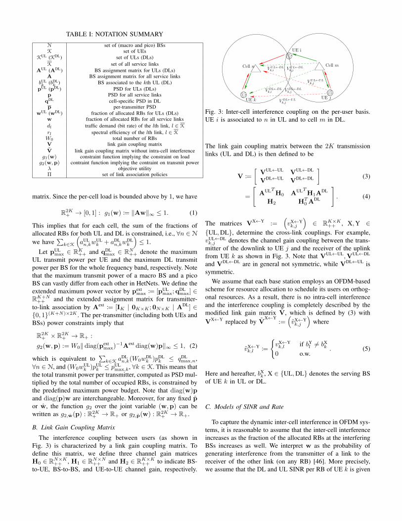
TABLE I: NOTATION SUMMARY

N set of (macro and pico) BSsK set of UEs

KUL (KDL) set of ULs (DLs)K set of all service links

AUL (ADL) BS assignment matrix for ULs (DLs)A BS assignment matrix for all service links

bULk (bDL

k ) BS associated to the kth UL (DL)pUL (pDL) PSD for ULs (DLs)

p PSD for all service linksqDL cell-specific PSD in DLp per-transmitter PSD

wUL (wDL) fraction of allocated RBs for ULs (DLs)w fraction of allocated RBs for all service linksdl traffic demand (bit rate) of the lth link, l ∈ K

rl spectral efficiency of the lth link, l ∈ KW0 total number of RBsV link gain coupling matrixV link gain coupling matrix without intra-cell interference

g1(w) constraint function implying the constraint on loadg2(w,p) contraint function implying the contraint on transmit power

λ objective utilityΠ set of link association policies

matrix. Since the per-cell load is bounded above by 1, we have

R2K+ → [0, 1] : g1(w) := ‖Aw‖∞ ≤ 1. (1)

This implies that for each cell, the sum of the fractions ofallocated RBs for both UL and DL is constrained, i.e., ∀n ∈ N

we have∑k∈K

(aULn,kw

ULk + aDL

n,kwDLk

)≤ 1.

Let pULmax ∈ RK++ and qDL

max ∈ RN++ denote the maximumUL transmit power per UE and the maximum DL transmitpower per BS for the whole frequency band, respectively. Notethat the maximum transmit power of a macro BS and a picoBS can vastly differ from each other in HetNets. We define theextended maximum power vector by pext

max := [pULmax; qDL

max] ∈RK+N

++ and the extended assignment matrix for transmitter-to-link association by Aext := [IK | 0K×K ; 0N×K | ADL] ∈0, 1(K+N)×2K . The per-transmitter (including both UEs andBSs) power constraints imply that

R2K+ × R2K

+ → R+ :

g2(w,p) := W0‖ diag(pextmax)−1Aext diag(w)p‖∞ ≤ 1, (2)

which is equivalent to∑k∈K aDL

n,k(W0wDLk )pDL

k ≤ qDLmax,n,

∀n ∈ N, and (W0wULk )pUL

k ≤ pULmax,k, ∀k ∈ K. This means that

the total transmit power per transmitter, computed as PSD mul-tiplied by the total number of occupied RBs, is constrained bythe predefined maximum power budget. Note that diag(w)pand diag(p)w are interchangeable. Moreover, for any fixed por w, the function g2 over the joint variable (w,p) can bewritten as g2,w(p) : R2K

+ → R+ or g2,p(w) : R2K+ → R+.

B. Link Gain Coupling Matrix

The interference coupling between users (as shown inFig. 3) is characterized by a link gain coupling matrix. Todefine this matrix, we define three channel gain matricesH0 ∈ RN×K++ , H1 ∈ RN×N++ and H2 ∈ RK×K++ to indicate BS-to-UE, BS-to-BS, and UE-to-UE channel gain, respectively.

UE k

UE i

V DL←ULk,j

V DL←DLk,i , V DL←DL

k,j

V UL←ULk,j

Cell mCell n

UE j

V UL←DLk,i , V UL←DL

k,j

Fig. 3: Inter-cell interference coupling on the per-user basis.UE i is associated to n in UL and to cell m in DL.

The link gain coupling matrix between the 2K transmissionlinks (UL and DL) is then defined to be

V :=

[VUL←UL VUL←DL

VDL←UL VDL←DL

](3)

=

[AULTH0 AULTH1A

DL

H2 HT0 ADL

]. (4)

The matrices VX←Y :=(vX←Yk,j

)∈ RK×K++ , X,Y ∈

UL,DL, determine the cross-link couplings. For example,vUL←DLk,j denotes the channel gain coupling between the trans-

mitter of the downlink to UE j and the receiver of the uplinkfrom UE k as shown in Fig. 3. Note that VUL←UL,VUL←DL

and VDL←DL are in general not symmetric, while VDL←UL issymmetric.

We assume that each base station employs an OFDM-basedscheme for resource allocation to schedule its users on orthog-onal resources. As a result, there is no intra-cell interferenceand the interference coupling is completely described by themodified link gain matrix V, which is defined by (3) withVX←Y replaced by V

X←Y:=(vX←Yk,j

)where

vX←Yk,l :=

vX←Yk,l if bY

l 6= bXk

0 o.w.. (5)

Here and hereafter, bXk , X ∈ UL,DL denotes the serving BS

of UE k in UL or DL.

C. Models of SINR and Rate

To capture the dynamic inter-cell interference in OFDM sys-tems, it is reasonable to assume that the inter-cell interferenceincreases as the fraction of the allocated RBs at the interferingBSs increases as well. We interpret w as the probability ofgenerating interference from the transmitter of a link to thereceiver of the other link (on any RB) [46]. More precisely,we assume that the DL and UL SINR per RB of UE k is given

by (respectively)

SINRDLk :=

pDLk vDL←DL

k,k∑i∈K

vDL←DLk,i wDL

i pDLi +

∑j∈K

vDL←ULk,j wUL

j pULj + σ2

SINRULk :=

pULk vUL←UL

k,k∑i∈K

vUL←DLk,i wDL

i pDLi +

∑j∈K

vUL←ULk,j wUL

j pULj + σ2

where σ2 > 0 denotes the background-noise powerspectral density, which is assumed to be the same forall receivers. Let us define σ := σ212K , and collectthe uplink and downlink SINR in a vector SINR :=[SINRUL

1 ; . . . ; SINRULK ; SINRDL

1 ; . . . ; SINRDLK ] ∈ R2K

++. Using(3), (4), and (5), the above expressions of SINR can be writtenin a general form

SINRl(p,w) :=pl[

D−1(V diagpw + σ

)]l

, l ∈ K, (6)

where D := diagvUL←UL1,1 , . . . , vUL←UL

K,K , vDL←DL1,1 , vDL←DL

K,K ∈R2K

+ is a diagonal matrix. For l = 1, . . . ,K, (6) is equal tothe UL SINR, while the DL SINR is given by (6) for l =K + 1, . . . , 2K.

We further assume that the spectral efficiency (bit rate perRB) of the virtual UEs (includes both UL and DL transmis-sion) is a strictly increasing function of the SINR given by

rl(p,w) := B log2(1 + SINRl(p,w)), l ∈ K, (7)

where B denotes the effective bandwidth per RB.Given the per-UE uplink and downlink traffic demands (bit

rate) d := [dUL1 , . . . , dUL

K , dDL1 , . . . , dDL

K ]T ∈ R2K++, it follows

from (7) that the traffic demands are satisfied if and only if(note that wl ·W0 is equal to the number of RBs used by linkl)

wl ≥dl

W0rl(p,w), l ∈ K. (8)

Remark 2 (Full Overlap or Partial Overlap). The SINRmodeled in (6) is based on the strategy that each UL orDL transmission is allocated a number of RBs in a jointfrequency band for both UL and DL, regardless of the locationof the band. However, this may result in a full overlap offrequency bands used by UL and DL transmissions leading tohigh probability of inter-link interference. A more reasonablestrategy is to allow only partial overlap, as shown in Fig. 2,where the DL is preferred to allocated at the head of the bandwhile the UL at the tail of the band, or vice versa. In this case,the inter-link interference only exists on the overlapping band,and the above-presented model overestimates the probability ofreceiving inter-link interference. A more accurate readjustmentis to multiply the term of inter-link interference with anadditional overlap factor. Some possible methods to definethe overlap factor are given in Appendix A. In the remainderof this paper, the analysis and algorithms are still presentedwith the interference model in (6) for the simplicity of theform. However, without loss of generality, we can easily adjust

the model by introducing the overlap factor into the couplingmatrix V.

D. Link Association Policies

Assume that there are a finite set of link association policiesΠ := πm : m = 1, . . . ,M implemented in the network,which can be dynamically selected by an operator. Eachpolicy defines the BS-UE assignment matrices AUL(πm) andADL(πm), and further defines the link gain coupling matrixV(πm) and link gain matrix D(πm) in (6).

As examples, in the following we list one conventionalUL/DL coupled user association policy and two types ofdecoupled UL/DL link association policies, respectively.(1) CoUD: Conventional coupled UL/DL user associationbased on reference signal received power (RSRP) in DL isgiven by

bULk = bDL

k = arg maxn∈N

RSRPn,k, ∀k ∈ K. (9)

(2) DeUD O: Decoupled UL/DL link association assisted withcell selection offset [17]. A cell selection offset is added to thereference signals of the small cells to increase their coveragein UL in order to offload some traffic from the macro cell.This can be formalized as follows

bXk = arg max

n∈NRSRPn,k + offsetXn, ∀k ∈ K,X ∈ UL,DL

(10)where offsetXn > 0 (in dB) if X = UL and n is a small cell BSwith low transmit power; otherwise the offset is set to zero ifX = DL or n is a macro cell BS.(3) DeUD P: Decoupled UL/DL link association based on DLreceived power and UL pathloss respectively [15], where theassociation criteria in DL and UL are given by (respectively)

bDLk = arg max

n∈NRSRPn,k, (11)

bULk = arg max

n∈NPLn,k, ∀k ∈ K, (12)

where PLn,k denotes the pathloss estimate between BS n andUE k.

Note that in (10), by setting offsetXn = 0 for all n ∈ N

and X = UL, the association policy is equivalent to CoUD.And, by setting the offset (in dB) of the small cell BS in ULas the difference between the transmit power (in dBm) of themacro cell BS and the small cell BS, DeUD O is equivalentto DeUD P.

III. PROBLEM FORMULATION

To achieve the service-centric network fairness, we definethe objective utility λ to be the minimum level of QoS satis-faction among all links, where the level of QoS satisfaction isequal to the ratio of the per-link feasible transmission rate tothe required traffic demand. So we have

λ := minl∈K

W0wlrl(p,w)

dl, (13)

where rl(p,w) is given by (7).

Given a certain link association policy π′ and its correspond-ing UL(DL) assignment matrice AUL(π′)( ADL(π′)), couplingmatrix V(π′), and link gain matrix D(π′), the objective isto maximize the utility λ over the joint space of loads andpowers subject to the constraints on the maximum per-cell load(1) and the maximum per-transmitter power (2). Moreover, ifthe optimized utility satisfies λ ≥ 1, then the vector of link-specific traffic demands d is feasible; otherwise, the trafficdemand cannot be satisfied for every service link. Formally,the problem of interest in this paper can be stated as follows.

Problem 1

maxw∈R2K

+ ,p∈R2K+

λ (14a)

subject to w ≥ λf(p,w) (14b)

fl(p,w) :=dl

W0rl(p,w),∀l ∈ K (14c)

(1), (2), (14d)

where the vector function f : R2K+ → R2K

++ in (14b) is acollection of fl defined in (14c), i.e., f := [f1, . . . , f2K ]T . Theutility λ depends on the joint variable (w,p) ∈ R2K

+ × R2K+

in an inextricably intertwined manner, which is due to thenonlinear power and resource coupling relationship betweenlinks. We decompose Problem 1 into two subproblems inProblem 2b by alternately optimizing over w or p, and providecomputationally efficient locally optimal solution to Problem1, based on the optimal solution to each of the subproblems.

Problem 22a Given fixed p′ ∈ R2K

+ , find w′ := w′(p′) such that

w′ = arg maxw∈R2K

+

λ (15a)

subject to w ≥ λfp′(w) (15b)g1(w) ≤ 1, g2,p′(w) ≤ 1, (15c)

where fp′ , g1, and g2,p′ are obtained by replacing p withp′ in (14c), (1) and (2), respectively.

2b Given fixed w′ ∈ R2K+ satisfying g1(w′) ≤ 1, find p′ :=

p′(w′) such that

p′ = arg maxp∈R2K

+

λ (16a)

subject to w′ ≥ λfw′(p) (16b)g2,w′(p) ≤ 1, (16c)

where fw′ and g2,w′ are obtained by replacing w withw′ in (14c) and (2), respectively.

Prob.2a and Prob.2b are formulated in such a way that acommon desired utility λ is maximized subject to the commonload and power constraints. Thus, for a given link associationpolicy π′, by sequentially solving Prob.2a and Prob.2b, weimprove λ in each step and achieve a local optimum of λwith respect to π′.

In Section IV and V we provide the optimal solutionto Prob.2a and Prob.2b, respectively. The joint algorithm issummarized in Section VI.

IV. JOINT UPLINK AND DOWNLINK RESOURCEALLOCATION

In this section we develop the algorithms for joint UL/DLbandwidth allocation. In Section IV-A we develop an algo-rithm for Prob.2a in Prop. 1. Since a solution w to Prob.2amust fulfill maxg1(w), g2,p′(w) ≤ 1, some free resourcesmay still be available, i.e., g1(w) < 1 and g2,p′(w) = 1,even under optimal power allocation (in the sense of Prob.2a). Therefore, an additional step involving power scalingand bandwidth updating is introduced in Prop. 2 in SectionIV-B, to further improve the desired utility λ. Another caseof g1(w) = 1 and g2,p′(w) ≤ 1 is discussed in Prop. 3 inSection V.

A. Algorithm for Bandwidth Allocation

The following lemma proves a key property of the vectorfunction fp′ , which is necessary to solve Prob. 2a.

Lemma 1. Given a fixed power vector p′, the function fp′ :R2K

+ → R2K++ defined in Prob. 1 is a standard interference

function.

The definition and some selected properties of standardinterference function (SIF) are provided in Appendix B. Theproof of Lemma 1 following the proof of [38, Ex. 2] isprovided in Appendix C.

We further prove the following theorem.

Theorem 1. Suppose

• g(x) : Rk++ → R++ is monotonic, and homogeneous ofdegree 1 (i.e., g(αx) = αg(x) for all α > 0),

• f(x) : Rk+ → Rk++ is a SIF.

Then, for each θ > 0 there is exactly one eigenvector x′ ∈Rk++ and associate eigenvalue ρ′ of f such that ρ′x′ = f(x′)and g(x′) = θ. The repeated iteration

x(t+1) =θf(x(t))

g f(x(t)), t ∈ N, (17)

converges to the unique vector x′, which is called the fixedpoint of f . The associate eigenvalue is ρ′ = g f(x′)/θ.

The proof of Theorem 1 is referred to Appendix D. It isa direct extension of the proof of [35, Th. 3.2], where g wasdefined as any monotonic norm ‖ · ‖, while we define threeproperties monotonicity, homogeneity and positivity on Rk++.Note that the function in (17) ψ := θf/g f : Rk+ → Rk++ isnon-monotonic, while it preserves the property of scalabilityof the mapping f .

Using Lemma 1 and Theorem 1, we prove the followingproposition, which gives rise to an algorithmic solution toProb.2a.

Proposition 1. Given a fixed p′ ∈ R2K+ , let the set of solutions

to Prob.2a be denoted by Fw(p′). There exists one w′ ∈Fw(p′) such that w′ ≤ w for all w ∈ Fw(p′). Moreover, w′

is an eigenvector of fp′ satisfying maxg1(w′), g2,p′(w′) =

1 and can be obtained by performing the following fixed pointiteration:

w(t+1) =fp′(w

(t))

gp′ fp′(w(t)), t ∈ N, (18a)

where gp′(w) := maxg1(w), g2,p′(w). (18b)

The iteration in (18) converges to w′, and λp′ = 1/gp′ fp′(w

′).

Proof. In the following part of this proof, for simplicity ofnotation, we omit the dependency on p′, and denote f := fp′ ,g := gp′ and λ := λp′ .

It is obvious that g defined in (18b) is positive and homo-geneous of degree 1 on R2K

++. By virtue of Theorem 1 andLemma 1, we have that for θ = 1, there exist a unique fixedpoint w′ = λ′f(w′) such that g(w′) = 1, where λ′ can becomputed with iteration (18a).

Then we show that there exists no λ′′ > λ′ to satisfyw′′ ≥ λ′′f(w′′) and g(w′′) ≤ 1. We proceed by con-tradiction. Suppose that there exists a λ′′ > λ′ to satisfyw′′ ≥ λ′′f(w′′) such that g(w′′) ≤ 1. Let us define a functionf ′ := λ′f . Because f is a SIF, f ′ is also a SIF. We thenhave f ′(w′′) = λ′f(w′′) < λ′′f(w′′) ≤ w′′, i.e., w′′ is afeasible point with respect to the SIF f ′. Thus, the sequencestarting from w′′ decreases monotonically to w′ (by usingthe third property of SIF stated in Lemma 3). Then we havew′ ≤ f ′(w′′) < w′′. Since g(w) is monotone increasing onR2K

+ , we have g(w′′) > g(w′) = 1, which contradicts theearlier statement g(w′′) ≤ 1.

Knowing that λ′ is the maximum feasible utility, now weshow that for all w ∈ Fw(p′) satisfying w ≥ λ′f(w) =f ′(w), we have w′ ≤ w. Because f ′ is also a SIF, w ≥ f ′(w)implies that the sequence w decreases monotonically to w′

satisfying w′ = f ′(w′) = λ′f(w′). Thus., w′ ≤ w.

B. Optimization to Achieve Maximum Load

As aforementioned, Prop.1 provides an algorithm that con-verges to the optimal solution to Prob.2a. Let w′ be thissolution. Since maxg1(w′), g2,p′(w

′) = 1, it is possible thatg2,p′(w

′) = 1, while g1(w′) < 1, i.e., the maximum powerper transmitter is satisfied with equality, while free resourcesare still available. In this case, we propose an additional step tofurther optimize λ by iteratively scaling down the fixed powervector p′, until g1(w′) = 1 is achieved.

Proposition 2. Let w′ ∈ R2K+ be the solution to Prob.2a

and suppose that g2,p′(w′) = 1 and g1(w′) < 1. Starting

from p(0) = p′ and w(0) = w′, by iteratively performing thefollowing two steps:(1) scaling down p by

p(t+1) = g1(w(t)) · p(t), (19)

(2) updating w(t+1), as the unique fixed point of iteration(18), with updated p′ = p(t+1),

the sequence of utility λ is monotone increasing, until themaximum load constraint g1(w) = 1 is satisfied.

The proof of Prop. 2 is provided in Appendix E.The optimization step provided in Prop. 2 further improves

our desired utility λ if the solution to Prob.2a w′ satisfiesg2,p′(w

′) = 1 and g1(w′) < 1. Now assume the algorithmdefined in Prop. 2 converges to (p?,w?). Then, in addition tothe full utilization of resources in the sense that g1(w?) = 1,we have g2(p?,w?) ≤ 1 = g2,p′(w

′), which means that theallocation obtained under Prop. 1 is more power efficient thanthat of Prop. 1.

Remark 3. It is worth mentioning that Ho [41] formulates apower minimization problem, based on the cell-specific loadand power coupling in the DL, and concludes that if theminimum required rate is feasible, then the optimal solutionto the power minimization problem satisfies that the system isfully loaded [41, Th. 1]. In this paper, we formulate a utilitymaximization problem, based on the link-specific bandwidthand power coupling framework in joint UL/DL, with per-cellload and per-transmitter power constraints, and conclude thatif some minimum utility is feasible with cell load lower thanone, we can scale down the power vector using the algorithmpresented in Prop. 2, to further increase the desired utility,until the per-cell load constraint holds with equality.

V. JOINT UPLINK AND DOWNLINK POWER CONTROL

Now let us consider the problem of power control. Inthis section, we first present the optimal solution to Prob.2bintroduced in Section V-A. Then, in Section V-B and V-C,we further examine two alternative algorithms for cell-specificpower control and energy efficient power control, respectively.

A. Algorithm for Link-Specific Power Control

Let us first consider Prob.2b. Given some fixed w′ ∈[0, 1]2K , we first rewrite the rate constraints in (16b). Forp ∈ R2K

++, we have

w′ ≥ λfw′(p)⇔ pl ≥ λplfw′,l(p)

w′lfor l ∈ K. (20)

We further define the following vector function using (20)

fw′ :R2K++ → R2K

++ : p 7→[fw′,1(p), . . . , fw′,2K(p)

]Twhere fw′,l(p) :=

plw′lfw′,l(p), l ∈ K. (21)

Note that the domain of fw′ defined in (21) is the positiveorthant R2K

++. To extend it to the non-negative orthant R2K+ ,

we define the following extension for each l ∈ K:

f ′w′,l(p) :=

fw′,l, if pl 6= 0dl ln 2

W0Bw′lIw′,l(p) o.w.

, (22)

where Iw′,l(p) :=[D−1

(V diagw′p + σ

)]l. (23)

The domain extension is derived by leveraging the linearapproximation log2(1 + x) ≈ x/ ln 2 for x → 0. As shownin (22), this approximation is only used for pl = 0 (which

further leads to SINRl = 0), otherwise if pl 6= 0, the nonlinearclosed-form of fw′,l (21) is used.

With (20), (22), and (23), Prob.2b is rewritten as

maxp∈R2K

+

λ, s.t. p ≥ λf ′w′(p), g2,w′(p) ≤ 1 (24)

The following lemma shows that f ′w′ has the same keyproperty as fp′ , which is shown for fp′ in Lemma 1.

Lemma 2. The vector function f ′w′ : R2K+ → R2K

++ defined in(22) is SIF.

Proof. The proof follows directly from the previous resultsin [40, Prop. 1], where a cell-specific utility function overthe cell-specific power vector in DL is shown to be positiveconcave, and thus a SIF [38, Prop. 1]. It is easy to see that ourdefined link-specific function f ′π′,w′ shares the same form withthe cell-specific function introduced in [40, Prop. 1]. Thus, weomit the details here and conclude that it is also a SIF.

Note that in the expression of per-transmitter power con-straint (2), the term diag(w)p and diag(p)w are interchange-able. With some fixed w′, the function g2,w′ defined in (24)is positive and homogeneous of degree 1 on R2K

++. Thus, byleveraging Lemma 2 and Theorem 1, we can argue alongsimilar lines as in Prop. 1 to conclude the following: startingfrom an arbitrary p(1) ∈ R2K

+ , the following fixed pointiteration

p(t+1) =f ′w′(p

(t))

g2,w′ f ′w′(p(t))

, t ∈ N (25)

converges to the solution of Prob.2b, denoted by p′′. And theutility λp′′ corresponding to p′′ is given by λp′′ = 1/g2,w′ f ′w′(p

′′).Using (25), we can iteratively approach arbitrarily close to

solution to Prob.2b given fixed w′ as the solution to Prob.2a.However, for joint optimization over (w,p), we are interestedin whether or not this solution further improves the desiredutility derived from the solution to Prob.2a. We present therelationship between λ′′ := λp′′ and λ′ := λp′ in Prop. 3.

Proposition 3. For some fixed p′, let w′ ∈ R2K++ be the

solution to Prob.2a and λ′ the corresponding utility. Moreover,given w′, let p′′ ∈ R2K

++ be the solution to Prob.2b and λ′′ thecorresponding utility. Then, λ′ and λ′′ are related as follows.• If g2,p′(w

′) = 1, then, we have λ′′ = λ′ and p′′ = p′

• If g2,p′(w′) < 1, then, we have λ′′ > λ′

The proof of Prop. 3 can be found in Appendix F.Prop. 3 implies that given the solution (w′,p′) derived from

the bandwidth updating step (Prop. 1) or the power scalingstep (Prop. 2), with fixed w′ at hand, solving Prob.2b (byperforming (25) ) can further improve the desired utility onlyif g2,p′(w

′) < 1; otherwise if g2,p′(w′) = 1 the solution to

Prob.2b with respect to w′ is equivalent to p′.

Remark 4. In this section, we rewrite the rate constraintsw′ ≥ λfp(w′) in Prob. 2b into a system of nonlinearinequalities p ≥ λf ′w′(p) as shown in (20)-(23). Hence both

the fixed point iterations in (18) and (25) (to solve Prob.2a and Prob. 2b, respectively) converge to the solutions thatmaximize the same λ defined in Prob. III. Note that if we treatthe power control problems separately, as stated for instancein [47], the rate constraint rl(p,w′) ≥ λdl/(w

′lW0) for all

l ∈ K can be directly translate into a SINR constraint bytaking the exponential function of both sides. We write (20)into a system of linear inequalities in powers:

pl ≥ η(λ)f′′

w′(p)

where η(λ) := 2λdl

W0Bw′l − 1 is monotone increasing for any

λ ∈ R2K+ , and f

′′

w′ : R2K+ → R2K

++ is of form of an affinetransformation p 7→ D−1

(V diag(w′)p + σ

). We can agree

along similar lines as in Prop. 1 to maximize η by performingthe fixed point iteration p = f

′′

w′(p)/(g2,w′ f′′

w′(p)) and thusindirectly maximize λ.

B. Algorithm for Cell-Specific Power Control

So far we have considered the case that the PSD p can bespecified per service link. In the practical system, however, inDL a transmitter determines constant cell-specific energy perresource element across all DL bandwidth and subframes untilit needs to be updated [48], while in UL a distinct transmissionpower can be assigned to each UE. Without loss of generality,the developed power control algorithm can be easily modifiedto meet this practical requirement. The objective is to optimizethe per-transmitter PSD as a collection of the per-UE UL andper-BS DL power vectors

p := [pUL; qDL]T ∈ RK+N+ , (26)

where qDL ∈ RN+ is the cell-specific PSD in DL, and the nthentry of qDL

l denotes the PSD of all the DLs associated to celln. Since all DLs served by the same cell share the same PSD,we have

pDL = ADLTqDL. (27)

The transformation between p and p is then given by

p = Λp, with Λ :=

[IK 0K×N

0K×K ADLT

]. (28)

In the following, we collect the per-UE rate constraint inUL and per-cell sum rate constraint in DL depending on p ina set of K + N nonlinear inequalities, where for j ∈ K thejth inequality implies the UL rate constraint for UE j, whilefor j ∈ N := K + 1, . . . ,K +N, the jth inequality impliesthe DL sum rate constraint for cell n = j −K.

1) Per-UE Rate Constraint in Uplink: Substituting (28) into(6), SINR of UE j in UL is simply given by

SINRj(p,w′) :=

pj

Iw′,j(p), for j ∈ K, (29)

where Iw′,j(p) :=[D−1

(V diagw′Λp + σ

)]j. (30)

Substituting (29) into (7) and (8), the per-UE rate constraintin UL depending on p is given by

pj ≥pjwj· djW0rj(p,w′)

=: fw′,j(p), for j ∈ K. (31)

2) Per-Cell Sum Rate Constraint in Downlink: Substituting(28) into (6), the DL SINR of UE k associated with cell n(depending on p) can be rewritten as:

SINRDLn,l(p,w

′) :=pK+n

Iw′,l(p), ∀l ∈ K

DLn , (32)

where Iw′,l(p) is defined in (30), KDLn denotes the set of DL

transmissions associated with cell n, and pK+n as the (K +n)th entry of p denotes the PSD in DL in cell n.

The spectral efficiency of UE k associated with cell n inDL and denoted by rDL

n,l(p,w′) is computed by substituting

(32) into (7). Then, using (8), the sum rate constraint per cellin DL (depending on p) yields

ν′n =∑l∈KDL

n

w′l ≥∑l∈KDL

n

dlW0rDL

n,l(p,w′), ∀n ∈ N (33)

⇒ pj ≥pj

ν′j−K

∑l∈KDL

j−K

dlW0rDL

j−K,l(p,w′)

=: fw′,j(p), for j ∈ N (34)

where ν′n denotes fraction of the total allocated RBs of cell nin DL, note that for j ∈ N, the jth entry of p is equal to thePSD of cell n = j −K in DL.

Note that (34) defines the jth entry of function fw′,j forj = K+1, . . . ,K+N , while for j = 1, . . . ,K, the expressionof fw′,j is given in (31).

3) Joint Downlink Cell-Specific and Uplink UE-specificPower Control: With (31) and (34) in hand, using the sametechniques as shown in (20)-(23), the optimization problem iswritten as

maxp∈RK+N

+

λ, s.t. p ≥ λfw′(p), g2,w′(p) ≤ 1 (35)

where g2,w′(p) is obtained by substituting (28) into (2), andfw′(p) is given by

fw′,j(p) :=

fw′,j(p) if pj 6= 0dl ln 2

W0Bw′jIw′,j(p) if pj = 0, j ∈ K∑

l∈KDLj−K

dl ln 2

W0Bν′j−KIw′,l(p) if pj = 0, j ∈ N

(36)

Proceeding long similar lines as in Lemma 2, it is easy to showthat fw′ : RK+N

+ → RK+N++ is SIF, while g2,w′ : RK+N

++ →R++ is monotonic and homogeneous with degree 1. Therefore,we can compute the solution to (35) by means of the fixedpoint iteration in (25), and with f ′w′(p) replaced by fw′(p).

C. Algorithm for Energy Efficient Power Control

If the following assumption holds, the rate requirements arestrictly feasible for all UL and DL transmissions.

Assumption 1. The solution to Prob. 2 (w?,p?) satisfies λ? >1.

Under Assumption 1, the problem of interest in the contextof energy efficient networks is that, instead of consuming highenergy to achieve λ > 1, how to minimize the sum transmitpower, such that the per-link rate constraint is just satisfied,i.e., λ = 1. The power minimization problem subjected to therate and power constraints are defined in Problem 3

Problem 3

minp∈R2K

+

ψ(p), s.t. p ≥ f ′w?(p), g2,w?(p) ≤ 1 (37)

where ψ : R2K+ → R+ can be any monotonic function (in each

coordinate, i.e., ψ(x) ≥ ψ(y) if xi ≥ yi for each i) that is non-decreasing. For example, by setting ψ(p) = ‖ diagw?p‖1,we aim at minimizing the sum transmit power over all occu-pied RBs and all transmitters.

Since f ′w? is SIF, Prob. 3 is a classical power minimizationproblem introduced in [22], and we provide the solution inProp. (4). We omit the proof because it follows directly from[22, Thm. 2].

Proposition 4. Under Assumption 1, the fixed point iteration

p(t+1) = f ′w?(p(t)

), t ∈ N (38)

converges to the optimum solution p?? to Prob. 3.

Note that without loss of generality, (37) can be easilytranslated to the power minimization problem over p bysubstituting (28) into (37) and replacing f ′w? with fw′ .

VI. ALGORITHM FOR JOINT OPTIMIZATION

Now we provide an algorithm for joint optimization ofbandwidth allocation w and power control p per link, withrespect to any fixed link association policy π′ ∈ Π. Based onProp. 1, 2, and 3, we can compute the locally optimum of(w(π′),p(π′)). In the following we explain in more detail thethree main steps (S1, S2 and S3) of the algorithm.

S1. Updating Bandwidth

The algorithm starts with optimizing the bandwidth allocationw, given an initial PSD p′. Prop. 1 provides the optimalsolution w′ in the sense of maximizing λ for any fixedp′. The algorithm converges to a solution w′, satisfyingmaxg1(w′), g2,p′(w

′) = 1, i.e., either g1(w′) = 1, org2,p′(w

′) = 1, or both. Therefore, it remains to consider thefollowing three cases(1) g1(w′) < 1 and g2,p′(w

′) = 1(2) g1(w′) = 1 and g2,p′(w

′) < 1(3) g1(w′) = 1 and g2,p′(w

′) = 1

Note that once the third condition is achieved, (w′,p′) is alocal optimum. In contrast, in the first case and the secondcase the algorithm is designed to further improve the utility

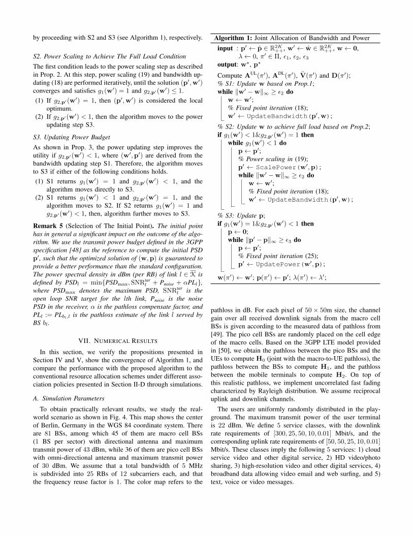
by proceeding with S2 and S3 (see Algorithm 1), respectively.

S2. Power Scaling to Achieve The Full Load Condition

The first condition leads to the power scaling step as describedin Prop. 2. At this step, power scaling (19) and bandwidth up-dating (18) are performed iteratively, until the solution (p′,w′)converges and satisfies g1(w′) = 1 and g2,p′(w

′) ≤ 1.(1) If g2,p′(w

′) = 1, then (p′,w′) is considered the localoptimum.

(2) If g2,p′(w′) < 1, then the algorithm moves to the power

updating step S3.

S3. Updating Power Budget

As shown in Prop. 3, the power updating step improves theutility if g2,p′(w

′) < 1, where (w′,p′) are derived from thebandwidth updating step S1. Therefore, the algorithm movesto S3 if either of the following conditions holds.(1) S1 returns g1(w′) = 1 and g2,p′(w

′) < 1, and thealgorithm moves directly to S3.

(2) S1 returns g1(w′) < 1 and g2,p′(w′) = 1, and the

algorithm moves to S2. If S2 returns g1(w′) = 1 andg2,p′(w

′) < 1, then, algorithm further moves to S3.

Remark 5 (Selection of The Initial Point). The initial pointhas in general a significant impact on the outcome of the algo-rithm. We use the transmit power budget defined in the 3GPPspecification [48] as the reference to compute the initial PSDp′, such that the optimized solution of (w,p) is guaranteed toprovide a better performance than the standard configuration.The power spectral density in dBm (per RB) of link l ∈ K isdefined by PSDl = minPSDmax,SNRtar

l + Pnoise + αPLl,where PSDmax denotes the maximum PSD, SNRtar

l is theopen loop SNR target for the lth link, Pnoise is the noisePSD in the receiver, α is the pathloss compensate factor, andPLl := PLbl,l is the pathloss estimate of the link l served byBS bl.

VII. NUMERICAL RESULTS

In this section, we verify the propositions presented inSection IV and V, show the convergence of Algorithm 1, andcompare the performance with the proposed algorithm to theconventional resource allocation schemes under different asso-ciation policies presented in Section II-D through simulations.

A. Simulation Parameters

To obtain practically relevant results, we study the real-world scenario as shown in Fig. 4. This map shows the centerof Berlin, Germany in the WGS 84 coordinate system. Thereare 81 BSs, among which 45 of them are macro cell BSs(1 BS per sector) with directional antenna and maximumtransmit power of 43 dBm, while 36 of them are pico cell BSswith omni-directional antenna and maximum transmit powerof 30 dBm. We assume that a total bandwidth of 5 MHzis subdivided into 25 RBs of 12 subcarriers each, and thatthe frequency reuse factor is 1. The color map refers to the

Algorithm 1: Joint Allocation of Bandwidth and Power

input : p′ ← p ∈ R2K++, w′ ← w ∈ R2K

++, w← 0,λ← 0, π′ ∈ Π, ε1, ε2, ε3

output: w?, p?

Compute AUL(π′), ADL(π′), V(π′) and D(π′);% S1: Update w based on Prop.1;while ‖w′ −w‖∞ ≥ ε2 do

w← w′;% Fixed point iteration (18);w′ ← UpdateBandwidth(p′,w);

% S2: Update w to achieve full load based on Prop.2;if g1(w′) < 1&g2,p′(w

′) = 1 thenwhile g1(w′) < 1 do

p← p′;% Power scaling in (19);p′ ← ScalePower(w′,p);while ‖w′ −w‖∞ ≥ ε2 do

w← w′;% Fixed point iteration (18);w′ ← UpdateBandwidth(p′,w);

% S3: Update p;if g1(w′) = 1&g2,p′(w

′) < 1 thenp← 0;while ‖p′ − p‖∞ ≥ ε3 do

p← p′;% Fixed point iteration (25);p′ ← UpdatePower(w′,p);

w(π′)← w′; p(π′)← p′; λ(π′)← λ′;

pathloss in dB. For each pixel of 50× 50m size, the channelgain over all received downlink signals from the macro cellBSs is given according to the measured data of pathloss from[49]. The pico cell BSs are randomly placed on the cell edgeof the macro cells. Based on the 3GPP LTE model providedin [50], we obtain the pathloss between the pico BSs and theUEs to compute H0 (joint with the macro-to-UE pathloss), thepathloss between the BSs to compute H1, and the pathlossbetween the mobile terminals to compute H2. On top ofthis realistic pathloss, we implement uncorrelated fast fadingcharacterized by Rayleigh distribution. We assume reciprocaluplink and downlink channels.

The users are uniformly randomly distributed in the play-ground. The maximum transmit power of the user terminalis 22 dBm. We define 5 service classes, with the downlinkrate requirements of [300, 25, 50, 10, 0.01] Mbit/s, and thecorresponding uplink rate requirements of [50, 50, 25, 10, 0.01]Mbit/s. These classes imply the following 5 services: 1) cloudservice video and other digital service, 2) HD video/photosharing, 3) high-resolution video and other digital services, 4)broadband data allowing video email and web surfing, and 5)text, voice or video messages.

Longitude13.4 13.405 13.41 13.415 13.42 13.425 13.43 13.435

La

titu

de

52.505

52.51

52.515

52.52

52.525

-120

-100

-80

-60

-40

Fig. 4: DeUD-enabled wireless network. Macro BSs - bluesolid triangles; pico cells - blue hollow triangles; UEs - whitecircle with blue edge; downlink association - green dashedline; uplink association - red dashed line.

B. Convergence of The Algorithm

Let us first examine the convergence behavior of the algo-rithms presented in Prop. 1, 2 and 3 (corresponding to S1, S2,and S3) in Algorithm 1, respectively. In Fig.6 we verify thepropositions and show the convergence of the algorithm 1 withthe fixed association policy DeUD P, at a single simulationsnapshot (i.e., the users are assumed to be static within onetime interval). The number of users is K = 500. The desirednumerical precisions are set to εi = 1e− 7, for i = 1, 2, 3.

Fig. 6a illustrates the convergence behavior of three suc-cessive steps S1, S2, and S3. The algorithm starts at step S1,where g1(w(0)) < 1 and g2(p(0),w(0)) < 1. The initial powerp(0) is chosen as described in Rem. 5, where PSDmax = 12dBm, SNRtar = 12.2 dB, α = 1, and Pnoise = −121.45 dBm.The initial bandwidth allocation is defined as w(0) = 0. Afterperforming the fixed point iteration (18) at S1, it convergesto the fixed point w′ such that g2(p(0),w′) = 1 whileg1(w′) is extremely small (approximately 0.01). The algorithmmoves therefore to S2 of power scaling. The algorithm atS2 converges to the point (w′′,p′), where g1(w′) = 1 andg2(w′′,p′) < 1, which causes the algorithm to move to S3.By the end of S3, the fixed point iteration (25) converges top′′ such that g1(w′′) = g2(w′′,p′′) = 1, and the algorithmterminates. At each step, the iteration improves the desiredutility λ monotonically.

An interesting observation we have made concerning therelationship between per-cell power constraint and the feasibleutility is illustrated in Fig. 6b. The motivation is to find out thetradeoff between the power consumption and the improvementof the utility. Fig. 6b shows the increase of the utility aswe increase the power constraint factor θ (θ increases from0.01 to 1.01 with step size of 0.01), under different self-noise power σ. As shown in Thm. 1, θ is the scaling factorof the monotonic constraint g(x). As for S3, in particular, θis scaling factor of the maximum power constraint such thatg2,w′(p) ≤ θ. For small value of σ (i.e., in an interference-dominant system), small value of θ is sufficient for the feasible

Cell i

Cell j

UL to DLDL to UL

cDLi = ν

DLi = 0.7 c

ULi = ν

ULi = 0.3

cULj = ν

ULj = 0.7c

DLj = ν

DLj = 0.3

Fig. 5: One possible approach to estimate the overlap factorbased on the historical load measurements. The overlap factorbetween downlinks served by cell i and the uplinks served bycell j is computed by cDL

i cULj = 0.49, while the overlap factor

between the uplinks served by cell i and the downlinks servedby cell j is computed by cUL

i cDLj = 0.09.

utility, and increase of θ only leads to minor increase of utility(blue and red curves for the noise power of −121 dBm and−100 dBm, respectively). Conversely, for the large value of σ(i.e., in a noise-dominant system), increase of θ has a strongereffect on improving utility (green and black curves for thenoise power of −80 dBm and −70 dBm, respectively). Theabove observation can help us to choose a proper operationpoint, to provide a good tradeoff between the total powerconsumption and the desired utility.

Fig. 6c and 6d are provided to illustrate the performanceof algorithms presented in Section V-B and V-C. Fig. 6cshows a case that restricting cell-specific DL power resultsin approximately 16% degradation of utility achieved by UE-specific DL power. Fig. 6d shows a specific example thatfor a certain snap shot of the network, over 90% of powerconsumption can be saved if we only target at required utilityλ = 1 instead of the maximum feasible λ, by performing thestep of energy efficient power control presented in SectionV-C.

C. Network Performance Evaluation

1) Selection of Association Policy: Now let us examine theperformance of Algorithm 1 under different link associationpolicies. The set of association policies Π, including CoUD,DeUD O (with variety of offsets) and DeUD P as introducedin Section II-D, is defined as follows. Note that all macrocell BSs have maximum transmit power of 43 dBm, while allsmall cell BSs of 30 dBm. Thus, by setting offsetUL

n = 13dB for n as small cell BS, the policy DeUD O is equivalentto DeUD P, while by setting offsetUL

n = 0 for all n ∈ N,the policy DeUD O is equivalent to CoUD. The set of policyΠ is then defined as a set of DeUD O policies with offsets0, 1, 3, 5, . . . , 51 of the small cell BSs in UL, where 0corresponding to CoUD and 13 corresponding to DeUD P.

Fig. 7 shows the average performance of the algorithm undereach policy π ∈ Π using the Monte Carlo techniques. Werun 500 independent tests, with uniform user distribution of100 static users in each test. Fig. 7a shows the percentage ofthe counts that a fixed policy provides the utility among thetop three maximum utilities achieved by all policies. Fig. 7bshows the average utility of a fixed policy over the 500 tests

(the high value of utility is due to the lower number of theusers compared to Fig. 6). The following two observationsare made. 1) Proper selection of DeUD policy can achieveapproximately 2× improvements on desired utility, comparedagainst CoUD. 2) Although DeUD P is not always the bestpolicy that provides maximum utility, it has a high chance toprovide relatively good performance (approximately 73% ofcounts among the top three maximum utility). Thus, in casethe operator wants to save the computational cost of exhaustivesearching for optimal association policies, always selectingDeUD P provides a suboptimal compromises. However, weshall remind that in many cases, DeUD P is not the bestassociation policy with respect to maximizing the desiredutility, as shown in the two examples of the single trial inFig. 7c and Fig. 7d respectively.

2) Effects of Overlapping Uplink/Downlink FrequencyBands: Note that in Section VII-C1, the frequency bandallocation follows the rule that only partial overlap betweenUL/DL frequency band is allowed to mitigate the inter-linkinterference, as shown in Rem. 2. Computation of the overlapfactor is provided by Appendix A. Since the overlap factoris estimated based on the historical measurements, the actualutility λ derived using optimized (p,w) may not be as highas the computed λ in Algorithm 1. On the other hand, if fulloverlap is allowed (i.e., each transmission can be allocated toany of the RBs, regardless of whether it is in UL or DL), then,the overlap factor is one, and the utility achieved by Algorithm1 can be much lower due to the strong inter-link interference.

In Fig. 8a we show the utility achieved by our proposed jointUL/DL optimization algorithm (represented by “Jo”), with thestrategy of partial or full overlap. The three subplots fromleft to right illustrate the utility when the association poli-cies “Best”, “DeUD P”and “CoUD”are applied, respectively.Policy “Best” denotes the policy where the offset providesthe maximum value of λ, i.e., π? = arg maxπ∈Π λ(π). Forscenario of partial overlap, the blue dashed line expresses theoptimized λ computed with our algorithm, while the green andred solid lines express the actual λ in UL and DL, respectively.Although the algorithm aims at achieving fair user-specific ULand DL utility, a small gap between the UL and DL utility canbe observed due to the biased estimation of the overlap factor.For scenario of full overlap, the magenta solid line expressesthe achieved λ for both UL and DL. Because the interferencecoupling model in (6) is accurate under the assumption of fulloverlap, there is no gap between the computed λ and the actualachievable λ.

Furthermore, we make the following observations. 1) Usingoptimized (w,p) based on estimated overlap factor, we canachieve the actual utility in DL only about 2% − 3% lowerthan the computed maximum feasible λ from the proposedalgorithm, and in UL about 10%−30% lower. 2) By regulatingthe frequency band allocated to UL and DL transmission withpartial overlap, we achieve a 50% − 100% increase in utilitythan allowing the full overlap. 3) By enabling UL and DLdecoupling, we can achieve a two-fold increase in the utility,compared to CoUD. Although DeUD P may not be the best

association policies, it still provides 60%−75% increase. Thesame conclusion is reached by the analysis on associationpolicies in Section VII-C1.

3) Comparison against QoS-Based Proportional Fairness:We use the proportional fairness (PF) algorithm as a baselinefor evaluating the utility benefits provided by our algorithm.To provide a fair comparison between the PF algorithm andour proposed algorithm, instead of the rate-based PF algorithm[51], we replace the rate with the metric of level of QoS sat-isfaction, i.e., W0wlrl/dl for link l ∈ K presented in (13). Werun PF algorithm under default UL/DL bandwidth ratio underboth association policies CoUD and DeUD P, to compare withthe proposed joint UL/DL optimization algorithm. The defaultUL/DL bandwidth ratio is set to be 9 : 16, i.e., out of 25 RBs,9 of them are assigned for UL transmission while 16 for DLtransmission.

Fig. 8b shows the performance comparison between ourproposed algorithm and the PF algorithm under DeUD P andCoUD. Conventional PF algorithm achieves fairness in UL andDL independently, and the fixed ratio of UL/DL bandwidthratio causes a large gap between the achievable utility inUL and DL. Our proposed Algorithm 1 outperforms the PFalgorithm, in the sense that it jointly optimizes the level ofQoS satisfaction in UL and DL to the best closing levels. Theutility in UL achieves three-fold increase than the PF algorithmin both DeUD P and CoUD. We still observe a 20% − 50%increase in DL utility in DeUD P, while in CoUD we sacrificesome DL utility to achieve a higher gain in UL. However,as more UEs are served in the system, even in CoUD weachieve better utility in both UL and DL than the QoS-basedPF algorithm.

Another observation in reference to Fig. 8b is that, for bothalgorithms, by splitting the UL/DL access, the performancecan be further improved by about 60% − 70%. It is worthmentioning that the gain of UL/DL decoupling is not ashigh as expected in [14], [15] (more than two-fold increase).Our explanation is that although the strength of the usefulsignal is increased by offloading more uplinks in small cells,the received signal strength of the interference may also beincreased because the small cells are normally located on thecell edge. Therefore, it increases the need for the joint UL/DLoptimization algorithm allowing flexible UL/DL bandwidthratio, as we proposed in Algorithm 1.

VIII. CONCLUSION

We studied the utility maximization problem for the uplinkand downlink decoupling-enabled HetNet, to jointly optimizethe uplink and downlink bandwidth allocation and powercontrol, under different association policies. The utility ismodeled as the minimum level of the QoS satisfaction, toachieve fair service-centric performance. We develop a gen-eral model of inter-cell interference, that includes inter-linkinterference between uplink and downlink, with properties ofpower coupling and load coupling. Based on the interferencemodel, we develop a three-step optimization algorithm using

the fixed point approach for nonlinear operators with or with-out monotonicity. The algorithm benefits from the user-centriccontext-aware communication environment in 5G networks,adapts the bandwidth allocation and power spectral densityaccording to the channel condition and traffic demand in bothUL and DL, and achieves jointly optimized utility in bothUL and DL. Numerical results show that the performance ofour algorithm outperforms the QoS-based proportional fairnessalgorithm, and it is robust against heavily loaded system withhigh traffic demand.

APPENDIX

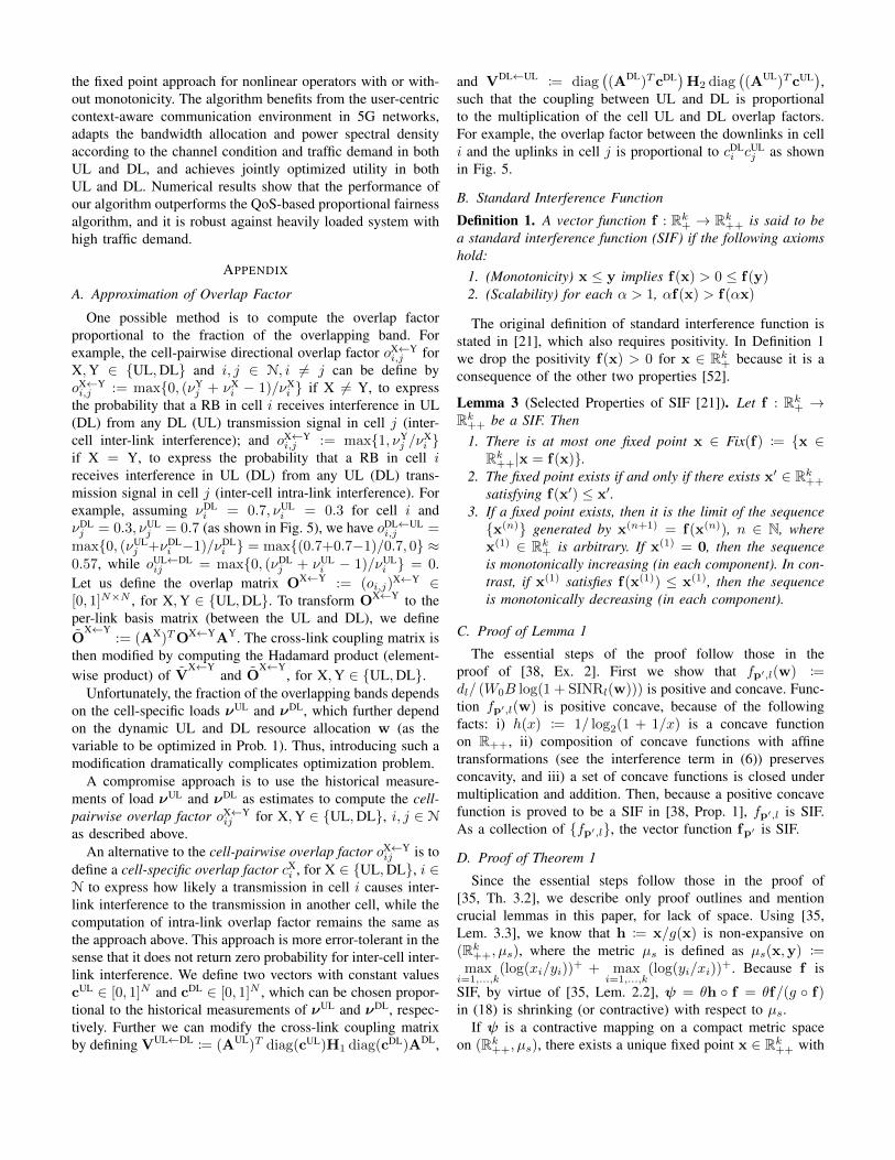
A. Approximation of Overlap Factor

One possible method is to compute the overlap factorproportional to the fraction of the overlapping band. Forexample, the cell-pairwise directional overlap factor oX←Y

i,j forX,Y ∈ UL,DL and i, j ∈ N, i 6= j can be define byoX←Yi,j := max0, (νY

j + νXi − 1)/νX

i if X 6= Y, to expressthe probability that a RB in cell i receives interference in UL(DL) from any DL (UL) transmission signal in cell j (inter-cell inter-link interference); and oX←Y

i,j := max1, νYj /ν

Xi

if X = Y, to express the probability that a RB in cell ireceives interference in UL (DL) from any UL (DL) trans-mission signal in cell j (inter-cell intra-link interference). Forexample, assuming νDL

i = 0.7, νULi = 0.3 for cell i and

νDLj = 0.3, νUL

j = 0.7 (as shown in Fig. 5), we have oDL←ULi,j =

max0, (νULj +νDL

i −1)/νDLi = max(0.7+0.7−1)/0.7, 0 ≈

0.57, while oUL←DLij = max0, (νDL

j + νULi − 1)/νUL

i = 0.Let us define the overlap matrix OX←Y := (oi,j)

X←Y ∈[0, 1]N×N , for X,Y ∈ UL,DL. To transform OX←Y to theper-link basis matrix (between the UL and DL), we defineO

X←Y:= (AX)TOX←YAY. The cross-link coupling matrix is

then modified by computing the Hadamard product (element-wise product) of V

X←Yand O

X←Y, for X,Y ∈ UL,DL.

Unfortunately, the fraction of the overlapping bands dependson the cell-specific loads νUL and νDL, which further dependon the dynamic UL and DL resource allocation w (as thevariable to be optimized in Prob. 1). Thus, introducing such amodification dramatically complicates optimization problem.

A compromise approach is to use the historical measure-ments of load νUL and νDL as estimates to compute the cell-pairwise overlap factor oX←Y

ij for X,Y ∈ UL,DL, i, j ∈ N

as described above.An alternative to the cell-pairwise overlap factor oX←Y

ij is todefine a cell-specific overlap factor cX

i , for X ∈ UL,DL, i ∈N to express how likely a transmission in cell i causes inter-link interference to the transmission in another cell, while thecomputation of intra-link overlap factor remains the same asthe approach above. This approach is more error-tolerant in thesense that it does not return zero probability for inter-cell inter-link interference. We define two vectors with constant valuescUL ∈ [0, 1]N and cDL ∈ [0, 1]N , which can be chosen propor-tional to the historical measurements of νUL and νDL, respec-tively. Further we can modify the cross-link coupling matrixby defining VUL←DL := (AUL)T diag(cUL)H1 diag(cDL)ADL,

and VDL←UL := diag((ADL)T cDL

)H2 diag

((AUL)T cUL

),

such that the coupling between UL and DL is proportionalto the multiplication of the cell UL and DL overlap factors.For example, the overlap factor between the downlinks in celli and the uplinks in cell j is proportional to cDL

i cULj as shown

in Fig. 5.

B. Standard Interference Function

Definition 1. A vector function f : Rk+ → Rk++ is said to bea standard interference function (SIF) if the following axiomshold:

1. (Monotonicity) x ≤ y implies f(x) > 0 ≤ f(y)2. (Scalability) for each α > 1, αf(x) > f(αx)

The original definition of standard interference function isstated in [21], which also requires positivity. In Definition 1we drop the positivity f(x) > 0 for x ∈ Rk+ because it is aconsequence of the other two properties [52].

Lemma 3 (Selected Properties of SIF [21]). Let f : Rk+ →Rk++ be a SIF. Then

1. There is at most one fixed point x ∈ Fix(f) := x ∈Rk++|x = f(x).

2. The fixed point exists if and only if there exists x′ ∈ Rk++

satisfying f(x′) ≤ x′.3. If a fixed point exists, then it is the limit of the sequencex(n) generated by x(n+1) = f(x(n)), n ∈ N, wherex(1) ∈ Rk+ is arbitrary. If x(1) = 0, then the sequenceis monotonically increasing (in each component). In con-trast, if x(1) satisfies f(x(1)) ≤ x(1), then the sequenceis monotonically decreasing (in each component).

C. Proof of Lemma 1

The essential steps of the proof follow those in theproof of [38, Ex. 2]. First we show that fp′,l(w) :=dl/ (W0B log(1 + SINRl(w))) is positive and concave. Func-tion fp′,l(w) is positive concave, because of the followingfacts: i) h(x) := 1/ log2(1 + 1/x) is a concave functionon R++, ii) composition of concave functions with affinetransformations (see the interference term in (6)) preservesconcavity, and iii) a set of concave functions is closed undermultiplication and addition. Then, because a positive concavefunction is proved to be a SIF in [38, Prop. 1], fp′,l is SIF.As a collection of fp′,l, the vector function fp′ is SIF.

D. Proof of Theorem 1

Since the essential steps follow those in the proof of[35, Th. 3.2], we describe only proof outlines and mentioncrucial lemmas in this paper, for lack of space. Using [35,Lem. 3.3], we know that h := x/g(x) is non-expansive on(Rk++, µs), where the metric µs is defined as µs(x,y) :=max

i=1,...,k(log(xi/yi))

+ + maxi=1,...,k

(log(yi/xi))+. Because f is

SIF, by virtue of [35, Lem. 2.2], ψ = θh f = θf/(g f)in (18) is shrinking (or contractive) with respect to µs.

If ψ is a contractive mapping on a compact metric spaceon (Rk++, µs), there exists a unique fixed point x ∈ Rk++ with

ψ(x) = x [36, Th.5.2.3]. In the following we show that ψ isa mapping of a compact space to itself. For any input, sinceg is homogeneous on Rk++, we have g ψ = (θ/g f) · (g f) = θ. Because a monotonic vector function has boundedlevel sets, we have that ψ(x) ≤ b for some finite b > 0.With ψ(x) ≤ b and f(x) ≥ f(0) for all x ∈ Rk+, we haveψ2(x) ≥ θf(0)/(g f(b)) = a > 0, and we see that therange of ψn falls inside the finite positive rectangle R(a,b)for n ≥ 2. Hence, there is exactly one eigenvector x ∈ Rk++

to satisfy x′ = ρ′f(x′) where the associate eigenvalue is givenby ρ′ = θ/(g f(x′)), such that g(x′) = g(ψ(x′)) = θ.

E. Proof of Prop. 2

We will prove by induction that by using algorithm in Prop.2, the sequence λ is monotonically increasing until g1(w) = 1is satisfied.

At the base step, suppose the solution to P.2a yieldsw′ = λ′fp′(w

′) where λ′ := 1/gp′(w′) and gp′(w

′) =maxg1(w′), g2,p′(w

′), with g1(w′) < 1 and g2,p′(w′) = 1.

Let us define g1(w′) = a < 1 and p′′ = ap′. With fixed p′′,using Theorem 1, iteration (18) converges to a unique fixedpoint w′′, satisfying

w′′ = λ′′fp′′(w′′) (39)

such that maxg1(w′′), g2(p′′,w′′) = 1 (40)

It is clear that fp′′(w′) < fp′(w

′) = w′/λ′, by di-viding both the numerator and denominator by a in (6),and substituting (6) in (7) and (14c). Now let us definev′ = w′/a > w′. Moreover, knowing that fp′′ is also aSIF, we have fp′′(v

′) = fp′′(w′/a) < fp′′(w

′)/a due tothe scalability, that further leads to fp′′(v

′) < fp′′(w′)/a <

fp′(w′)/a = w′/(aλ′) = v′/λ′. In other words, there exists

v′ such that λ′fp′′(v′) < v′, and v′ is a feasible point withrespect to the SIF f ′p′′ := λ′fp′′ . Thus, starting from v′, thesequence of v decrease monotonically to a unique fixed point(by using the third property of SIF stated in Lemma 3)

v′′ = f ′p′′(v′′) < f ′p′′(v

′) < v′ (41)

Due to the monotonicity and homogeneity of g1 with respectto w, and the same properties of g2 with respect to both pand w, we have

g1(v′′) < g1(v′) = g1(w′/a) = g1(w′)a = 1 (42)g2(p′′,v′′) < g2(ap′,v′) = g2(ap′,w′/a) = 1 (43)

We prove λ′′ > λ′ by contradiction. Suppose λ′′ ≤ λ′,then we have λ′′fp′′(v

′′) ≤ λ′fp′′(v′′) = v′′, using (41).

By defining f ′′p′′ := λ′′fp′′ which is also a SIF, sincef ′′p′′(v

′′) ≤ v′′, starting from v′′, the sequence of w is mono-tonically decreasing to the unique fixed point v? satisfyingv? = f ′′p′′(v

?) = λ′′fp′′(v?). Because v? is unique (by using

the first and second properties of SIF stated in Lemma 3),using (39), we have w′′ = v? ≤ v′′, which further leads tomaxg1(v′′), g2(p′′,v′′) ≥ maxg1(w′′), g2(p′′,w′′) = 1.This contradicts the inequalities (42) and (43). Thus, we havethat λ′′ > λ′ if g1(w′) < 1.

For the further iteration step, using (40), it remains toconsider cases in which g1(w′′) = 1, or g1(w′′) <1, g2(p′′,w′′) = 1. The former case directly leads tog1(w′′) = 1, and the algorithm stops at λ′′ > λ′. The lattercase yields g1(w′′) < 1, The proof above shows that the iter-ation step further increases λ, with scaled p′′′ = g1(w′′)p′′.

F. Proof of Prop. 3

The solution to P.2a satisfies p′ = λ′fw′(p′) using the

reformulation in (20). Since the variables p and w are in-terchangeable in g2, we have g2,p′(w

′) = g2,w′(p′).

Therefore, if g2,w′(p′) = 1, Theorem 1 implies that there is

exactly one eigenvector λ and associate eigenvector p of fw′

such that g2,w′(p′) = 1, and we have λ′′ = λ′ and p′′ = p′.

Then we consider the case when g2,w′(p′) < 1. Because

p′′ is the optimal solution to P.2b, if we can find a p ∈ R2K++

such that λ := minl∈K pl/fw′,l(p), g2,w′(p) ≤ 1 and λ > λ′,then we have λ′′ ≥ λ > λ′. Thus, the remaining task is to findan arbitrary p that fulfills the above mentioned conditions. Letus define α = 1/g2,w′(p

′) > 1 and p := ap′. Then, we have

λ = minl∈K

αp′lfw′,l(αp′)

> minl∈K

αp′lαfw′,l(p′)

= λ′

The above inequality is due to the scalability of the SIF fw′ .

ACKNOWLEDGMENT

We would like to thank Renato L.G. Cavalcante, CarlNuzman and Paolo Baracca for the numerous technical dis-cussions.

REFERENCES

[1] J. G. Andrews, “Seven ways that HetNets are a cellular paradigm shift,”Communications Magazine, IEEE, vol. 51, no. 3, pp. 136–144, 2013.

[2] F. Boccardi, R. W. Heath, A. Lozano, T. L. Marzetta, and P. Popovski,“Five disruptive technology directions for 5G,” Communications Maga-zine, IEEE, vol. 52, no. 2, pp. 74–80, 2014.

[3] Telecom Italia, “Big data challenge 2015,” 2015. [Online]. Available:http://www.telecomitalia.com/tit/it/bigdatachallenge.html

[4] G.-M. Su, Z. Han, M. Wu, and K. Liu, “Joint uplink and downlinkoptimization for real-time multiuser video streaming over WLANs,”Selected Topics in Signal Processing, IEEE Journal of, vol. 1, no. 2,pp. 280–294, 2007.

[5] M. Schubert and H. Boche, “Iterative multiuser uplink and downlinkbeamforming under SINR constraints,” Signal Processing, IEEE Trans-actions on, vol. 53, no. 7, pp. 2324–2334, 2005.

[6] A. M. El-Hajj, Z. Dawy, and W. Saad, “A stable matching game for jointuplink/downlink resource allocation in OFDMA wireless networks,” inCommunications (ICC), 2012 IEEE International Conference on. IEEE,2012, pp. 5354–5359.

[7] A. Abdel Khalek, L. Al-Kanj, Z. Dawy, and G. Turkiyyah, “Optimizationmodels and algorithms for joint uplink/downlink UMTS radio networkplanning with SIR-based power control,” Vehicular Technology, IEEETransactions on, vol. 60, no. 4, pp. 1612–1625, 2011.

[8] C.-H. Chiang, W. Liao, T. Liu, I. K. Chan, and H.-L. Chao, “Adaptivedownlink and uplink channel split ratio determination for TCP-basedbest effort traffic in TDD-based WiMax networks,” Selected Areas inCommunications, IEEE Journal on, vol. 27, no. 2, pp. 182–190, 2009.

[9] S. Kaur, A. Reznik, and D. R. Castor, “Method and apparatus for amulti-radio access technology layer for splitting downlink-uplink overdifferent radio access technologies,” Aug. 20, 2010, US Patent App.12/859,863.

[10] X. Chen and R. Hu, “Joint uplink and downlink optimal mobile associ-ation in a wireless heterogeneous network,” in Global CommunicationsConference (GLOBECOM), 2012 IEEE. IEEE, 2012, pp. 4131–4137.

[11] D. Liu, Y. Chen, K. K. Chai, and T. Zhang, “Backhaul aware joint uplinkand downlink user association for delay-power trade-offs in hetnets withhybrid energy sources,” Transactions on Emerging TelecommunicationsTechnologies, 2015.

[12] S. Kim and J.-W. Lee, “Joint resource allocation for uplink and downlinkin wireless networks: A case study with user-level utility functions,” inVehicular Technology Conference, 2009. VTC Spring 2009. IEEE 69th.IEEE, 2009, pp. 1–5.

[13] D. Astely, E. Dahlman, G. Fodor, S. Parkvall, and J. Sachs, “LTE release12 and beyond,” Communications Magazine, IEEE, vol. 51, no. 7, pp.154–160, 2013.

[14] F. Boccardi, J. Andrews, H. Elshaer, M. Dohler, S. Parkvall, P. Popovski,and S. Singh, “Why to decouple the uplink and downlink in cellularnetworks and how to do it,” arXiv preprint arXiv:1503.06746, 2015.

[15] H. Elshaer, F. Boccardi, M. Dohler, and R. Irmer, “Downlink anduplink decoupling: a disruptive architectural design for 5G networks,”in GLOBECOM’14. IEEE, 2014, pp. 1798–1803.

[16] ——, “Load & backhaul aware decoupled downlink/uplink access in 5Gsystems,” arXiv preprint arXiv:1410.6680, 2014.

[17] Qualcomm, “Range expansion for efficient support of heterogeneousnetworks,” 3GPP TSG-RAN WG1 R1-083813, 2008.

[18] K. Smiljkovikj, H. Elshaer, P. Popovski, F. Boccardi, M. Dohler,L. Gavrilovska, and R. Irmer, “Capacity analysis of decoupled down-link and uplink access in 5G heterogeneous systems,” arXiv preprintarXiv:1410.7270, 2014.

[19] K. Smiljkovikj, P. Popovski, and L. Gavrilovska, “Analysis of thedecoupled access for downlink and uplink in wireless heterogeneousnetworks,” Wireless Communications Letters, IEEE, vol. 4, no. 2, pp.173–176, 2015.

[20] S. Singh, X. Zhang, and J. G. Andrews, “Joint rate and SINR coverageanalysis for decoupled uplink-downlink biased cell associations inHetNets,” CoRR, vol. abs/1412.1898, 2014. [Online]. Available:http://arxiv.org/abs/1412.1898

[21] R. Yates, “A framework for uplink power control in cellular radiosystems,” IEEE J. Select. Areas Commun., vol. 13, no. 7, pp. 1341–1347, Sep. 1995.

[22] R. Yates and C. Huang, “Integrated power control and base stationassignment,” IEEE Trans. Veh. Technol., vol. 44, no. 3, pp. 638–644,Aug. 1995.

[23] S. Ulukus and R. Yates, “Stochastic power control for cellular radiosystems,” IEEE Trans. Commun., vol. 46, no. 6, pp. 784–798, 1998.

[24] J. Luo, S. Ulukus, and A. Ephremides, “Probability one convergence injoint stochastic power control and blind MMSE interference suppres-sion,” Positivity, vol. 1, p. 0, 2003.

[25] ——, “Standard and quasi-standard stochastic power control algo-rithms,” Information Theory, IEEE Transactions on, vol. 51, no. 7, pp.2612–2624, 2005.

[26] M. Chiang and J. Bell, “Balancing supply and demand of bandwidth inwireless cellular networks: utility maximization over powers and rates,”in INFOCOM 2004. Twenty-third Annual Joint Conference of the IEEEComputer and Communications Societies, vol. 4. IEEE, 2004, pp.2800–2811.

[27] H. Boche, M. Schubert, S. Stanczak, and M. Wiczanowski, “An ax-iomatic approach to resource allocation and interference balancing,” inProc. IEEE International Conference on Acoustics, Speech, and SignalProcessing (ICASSP), Philadelphia, PA, USA, March 18-23 2005.

[28] M. Schubert, H. Boche, and S. Stanczak, “Joint power control andmultiuser receiver design–fairness issues and cross-layer optimization,”in Proc. IST Summit 2005, Dresden, Germany, June 19-23 2005.

[29] H. Boche and M. Schubert, “The structure of general interferencefunctions and applications,” Information Theory, IEEE Transactions on,vol. 54, no. 11, pp. 4980–4990, 2008.

[30] S. Stanczak, M. Wiczanowski, and H. Boche, Fundamentals of resourceallocation in wireless networks: theory and algorithms. Springer, 2009,vol. 3.

[31] G. F. Frobenius, F. G. Frobenius, F. G. Frobenius, and F. G. Frobenius,Uber Matrizen aus nicht negativen Elementen. Konigliche Akademieder Wissenschaften, 1912.

[32] L. Zheng and C. W. Tan, “Optimal algorithms in wireless utility max-imization: Proportional fairness decomposition and nonlinear Perron-Frobenius theory framework,” Wireless Communications, IEEE Trans-actions on, vol. 13, no. 4, pp. 2086–2095, 2014.

[33] Y.-W. P. Hong, C. W. Tan, L. Zheng, C.-L. Hsieh, and C.-H. Lee, “Aunified framework for wireless max-min utility optimization with general

monotonic constraints,” in INFOCOM, 2014 Proceedings IEEE. IEEE,2014, pp. 2076–2084.

[34] B. Lemmens and R. Nussbaum, Nonlinear Perron-Frobenius Theory.Cambridge University Press, 2012, no. 189.

[35] C. J. Nuzman, “Contraction approach to power control, with non-monotonic applications,” in GLOBECOM’07. IEEE, 2007, pp. 5283–5287.

[36] D. R. Smart, Fixed point theorems. CUP Archive, 1980, no. 66.[37] I. Siomina and D. Yuan, “Load balancing in heterogeneous LTE:

Range optimization via cell offset and load-coupling characterization,” inCommunications (ICC), 2012 IEEE International Conference on. IEEE,2012, pp. 1357–1361.

[38] R. Cavalcante and et al., “Toward energy-efficient 5G wireless com-munication technologies,” Signal Processing Mag., vol. 31, no. 6, pp.24–34, 2014.

[39] C. K. Ho, D. Yuan, and S. Sun, “Data offloading in load coupled net-works: A utility maximization framework,” Wireless Communications,IEEE Transactions on, vol. 13, no. 4, pp. 1921–1931, 2014.

[40] R. L. Cavalcante, E. Pollakis, and S. Stanczak, “Power estimation in LTEsystems with the general framework of standard interference mappings,”in GlobalSIP’14. IEEE, 2014, pp. 818–822.

[41] C. Ho, D. Yuan, L. Lei, and S. Sun, “On power and load couplingin cellular networks for energy optimization,” IEEE Trans. WirelessCommun., 2014, accepted for publication.

[42] N. Alliance, “5G white paper,” Next Generation Mobile Networks, Whitepaper, 2015.

[43] E. Dahlman, G. Mildh, S. Parkvall, J. Peisa, J. Sachs, and Y. Selen, “5gradio access,” Ericsson Review, vol. 6, pp. 2–7, 2014.

[44] X. Zhang, J. Ming, and et al, “Filtered - OFDM - enabler for flexiblewaveform in the 5th generation cellular networks,” in Global Commu-nications Conference (GLOBECOM), 2015 IEEE. IEEE, 2015, pp.1–6.

[45] D. Bharadia, K. Joshi, and S. Katti, “Robust full duplex radio link,” inProceedings of the 2014 ACM conference on SIGCOMM. ACM, 2014,pp. 147–148.

[46] P. Mogensen, W. Na, I. Z. Kovacs, F. Frederiksen, A. Pokhariyal,K. Pedersen, T. Kolding, K. Hugl, M. Kuusela et al., “LTE capacitycompared to the shannon bound,” in Vehicular Technology Conference,2007. VTC2007-Spring. IEEE 65th. IEEE, 2007, pp. 1234–1238.

[47] H. Boche and M. Schubert, “Duality theory for uplink and down-link multiuser beamforming,” in Smart Antennas–State-of-the-Art, ser.EURASIP Book Series on Signal Processing and Communications.Hindawi Publishing Corporation, 2005, pp. 545–575.

[48] Evolved Universal Terrestrial Radio Access (E-UTRA), “Physical layerprocedures (Release 12),” 3GPP TS 36.213 V 12.7.0, 2015.

[49] MOMENTUM, “Models and simulations for network planning andcontrol of UMTS,” http://momentum.zib.de, 2004.

[50] 3GPP, “Evolved universal terrestrial radio access (E-UTRA);; furtheradvancements for E-UTRA physical layer aspects tr 36.814 v9.0.0(2010-03),” http://www.3gpp.org, 2010.

[51] T.-D. Nguyen and Y. Han, “A proportional fairness algorithm withQoS provision in downlink OFDMA systems,” IEEE CommunicationsLetters, vol. 10, no. 11, pp. 760–762, 2006.

[52] K. K. Leung, C. W. Sung, W. S. Wong, Lok, and Tat-Ming, “Con-vergence theorem for a general class of power-control algorithms,”Communications, IEEE Transactions on, vol. 52, no. 9, pp. 1566–1574,2004.

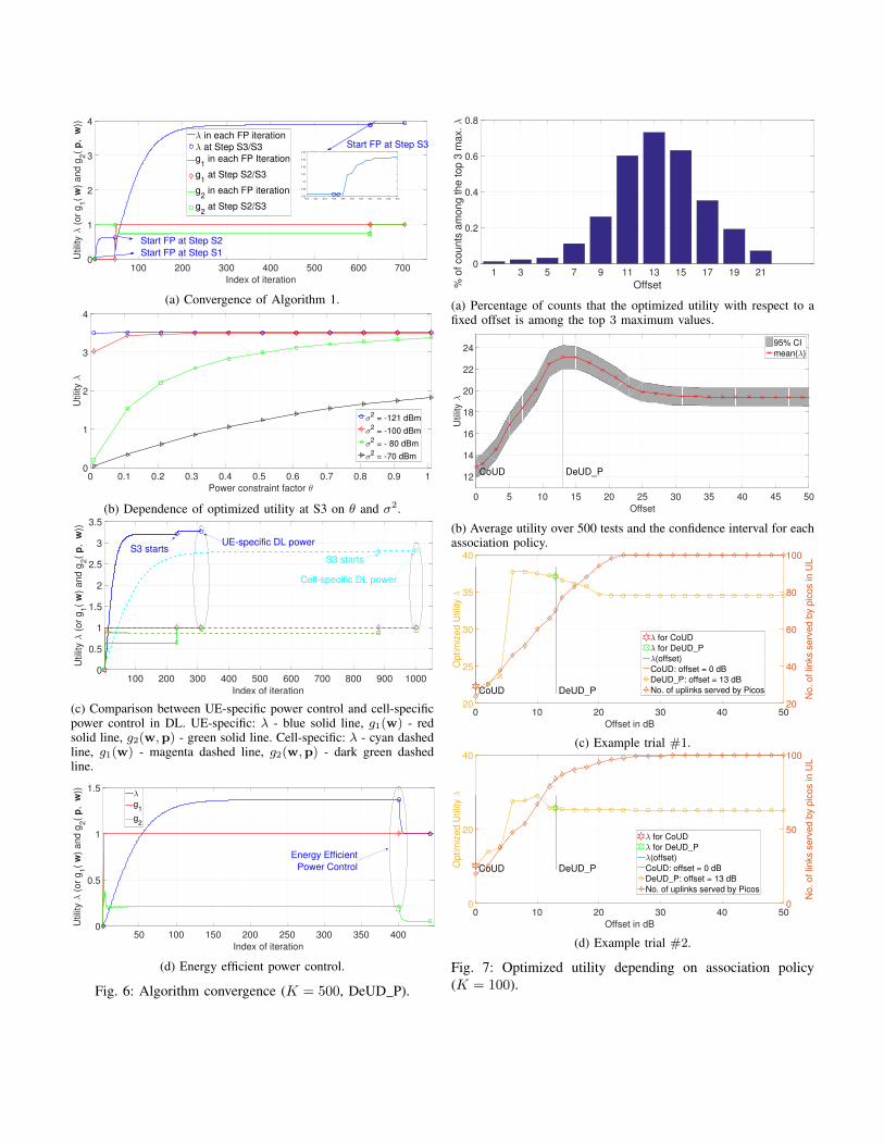
Index of iteration

100 200 300 400 500 600 700

Utilit

y λ

(o

r g

1(

w)

an

d g

2(

p,

w))

0

1

2

3

4

λ in each FP iteration

λ at Step S3/S3

g1 in each FP Iteration

g1 at Step S2/S3

g2 in each FP iteration

g2 at Step S2/S3

620 622 624 626 628 630 632 634 636 638 6403.88

3.89

3.9

3.91

3.92

3.93

3.94

Start FP at Step S1

Start FP at Step S3

Start FP at Step S2

(a) Convergence of Algorithm 1.

Power constraint factor θ

0 0.1 0.2 0.3 0.4 0.5 0.6 0.7 0.8 0.9 1

Utilit

y λ

0

1

2

3

4

σ2 = -121 dBm

σ2 = -100 dBm

σ2 = - 80 dBm

σ2 = -70 dBm

(b) Dependence of optimized utility at S3 on θ and σ2.

Index of iteration

100 200 300 400 500 600 700 800 900 1000

Utilit

y λ

(or

g1(

w)

and g

2(

p,

w))

0

0.5

1

1.5

2

2.5

3

3.5

UE-specific DL powerS3 starts

S3 starts

Cell-specific DL power

(c) Comparison between UE-specific power control and cell-specificpower control in DL. UE-specific: λ - blue solid line, g1(w) - redsolid line, g2(w,p) - green solid line. Cell-specific: λ - cyan dashedline, g1(w) - magenta dashed line, g2(w,p) - dark green dashedline.

Index of iteration

50 100 150 200 250 300 350 400

Utilit

y λ

(o

r g

1(

w)

an

d g

2(

p,

w))

0

0.5

1

1.5λ

g1

g2

Energy Efficient

Power Control

(d) Energy efficient power control.

Fig. 6: Algorithm convergence (K = 500, DeUD P).

Offset

1 3 5 7 9 11 13 15 17 19 21

% o

f counts

am

ong the top 3

max. λ

0

0.2

0.4

0.6

0.8

(a) Percentage of counts that the optimized utility with respect to afixed offset is among the top 3 maximum values.

Offset

0 5 10 15 20 25 30 35 40 45 50

Utilit

y λ

12

14

16

18

20

22

24

CoUD DeUD_P

95% CI

mean(λ)

(b) Average utility over 500 tests and the confidence interval for eachassociation policy.

Offset in dB

0 10 20 30 40 50

Op

tim

ize

d U

tilit

y λ

20

25

30

35

40

CoUD DeUD_P

No

. o

f lin

ks s

erv

ed

by p

ico

s in

UL

20

40

60

80

100

λ for CoUD

λ for DeUD_P

λ(offset)

CoUD: offset = 0 dB

DeUD_P: offset = 13 dB

No. of uplinks served by Picos

(c) Example trial #1.

Offset in dB

0 10 20 30 40 50

Op

tim

ize

d U

tilit

y λ

0

20

40

CoUD DeUD_P

No

. o

f lin

ks s

erv

ed

by p

ico

s in

UL

0

50

100

λ for CoUD

λ for DeUD_P

λ(offset)

CoUD: offset = 0 dB

DeUD_P: offset = 13 dB

No. of uplinks served by Picos

(d) Example trial #2.

Fig. 7: Optimized utility depending on association policy(K = 100).

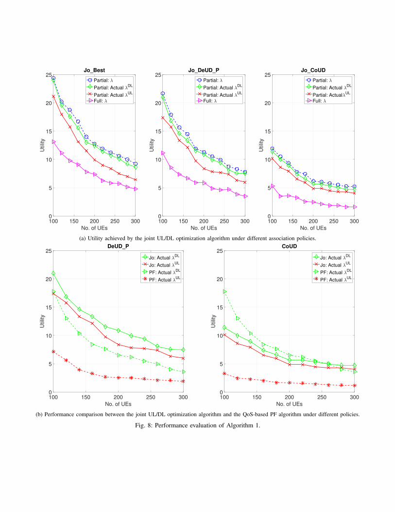
No. of UEs

100 150 200 250 300

Utilit

y

0

5

10

15

20

25Jo_Best

Partial: λ

Partial: Actual λDL

Partial: Actual λUL

Full: λ

No. of UEs

100 150 200 250 300

Utilit

y

0

5

10

15

20

25Jo_DeUD_P

Partial: λ

Partial: Actual λDL

Partial: Actual λUL

Full: λ

No. of UEs

100 150 200 250 300

Utilit

y

0

5

10

15

20

25Jo_CoUD

Partial: λ

Partial: Actual λDL

Partial: ActualλUL

Full: λ

(a) Utility achieved by the joint UL/DL optimization algorithm under different association policies.

No. of UEs

100 150 200 250 300

Utilit

y

0

5

10

15

20

25DeUD_P

Jo: Actual λDL

Jo: Actual λUL

PF: Actual λDL

PF: Actual λUL

No. of UEs

100 150 200 250 300

Utilit

y

0

5

10

15

20

25CoUD

Jo: Actual λDL

Jo: Actual λUL

PF: Actual λDL

PF: Actual λUL

(b) Performance comparison between the joint UL/DL optimization algorithm and the QoS-based PF algorithm under different policies.

Fig. 8: Performance evaluation of Algorithm 1.