ED 478 412

AUTHOR

TITLE

INSTITUTIONREPORT. NO

PUB DATE

NOTE

AVAILABLE FROM

PUB TYPEEDRS PRICEDESCRIPTORS

IDENTIFIERS

ABSTRACT

DOCUMENT RESUME

UD 035 816

Fairlie, Robert W.

The Effects of Home Computers on School Enrollment. JCPRWorking Paper.

Joint Center for Poverty Research, IL.JCPR-WP-3372003-06-0032p.

University of Chicago, Joint Center for Poverty Research,1155 E. 60th Street, Chicago, IL 60637. Tel: 773-702-0472;Fax: 773-702-0926; Web site: http://wwww.jcpr.org.Reports Research (143)

EDRS Price MF01/PCO2 Plus Postage.

*Access to Computers; *Computer Uses in Education; DropoutPrevention ; Dropout Research; *Enrollment Trends; *HighSchool Students; Internet; Secondary Education*Home Computers

Approximately 9 out of 10 high school students who haveaccess to a home computer use that computer to complete school assignments.Using. the. Computer and Internet Use Supplements to the 2001 CurrentPopulation Survey, this study explores whether access to home computersincreases the likelihood of school enrollment among teenagers who have notgraduated from high school. A comparison of school enrollment rates revealsthat 95.2 percent of children who have home computers are enrolled in school,whereas only 85.4 percent of children who do not have home computers areenrolled in school. Results find a difference of roughly 7.7 percentagepoints in school enrollment rates after estimating a bivariate probit modelfor the joint probability of school enrollment and owning a home computer.Use of computers and the Internet by the child's mother and father are usedas instrumental variables. These variables should affect computer ownership,but not school enrollment (after controlling for family income, parentaleducation, and parental occupation). The estimates are not sensitive toalternative combinations of instruments and different samples. The resultsprovide evidence that home computers increase the likelihood of staying inschool. (Contains 34 references.) (Author/SM)

Reproductions supplied by EDRS are the best that can be madefrom the on inal document.

N

U.S. DEPARTMENT OF EDUCATIONOffice of Educational Research and Improvement

EDUCATIONAL RESOURCES INFORMATIONCENTER (ERIC)

ellhis document has been reproduced asreceived from the person or organizationoriginating it.

Minor changes have been made toimprove reproduction quality.

Points of view or opinions stated in thisdocument do not necessarily represent00 official OERI position or policy.

1

The Effects of Home Computers on School Enrollment

Robert W. Fair lieUniversity of California, Santa Cruz

May 2003

PERMISSION TO REPRODUCE ANDDISSEMINATE THIS MATERIAL HAS

BEEN GRANTED BY

WiV 0:EaliCOLy-i-37a-fLi

TO THE EDUCATIONAL RESOURCESINFORMATION CENTER (ERIC)

I would like to thank Lori Kletzer, Federico Ravenna, Ron Grieson and seminarparticipants at BALE at UCSF for helpful comments and suggestions. Garima Vasishthaprovided excellent research assistance.

2 31ST COPY MAMIE

Abstract

Approximately 9 out of 10 high school students who have access to a home computer usethat computer to complete school assignments. Do these home computers, however,improve educational outcomes? 'Using the Computer and Internet Use Supplement to the2001 Current Population Survey, I explore whether access to home computers increasesthe likelihood of school enrollment among teenagers who have not graduated from highschool. A comparison of school enrollment rates reveals that 95.2 percent of childrenwho have home computers are enrolled in school, whereas only 85.4 percent of childrenwho do not have home computers are enrolled in school. I find a difference of roughly7.7 percentage points in school enrollment rates after estimating a bivariate probit modelfor the joint probability of school enrollment and owning a home computer. Use ofcomputers and the Internet by the child's mother and father are used as instrumentalvariables. These variables should affect computer ownership, but not school enrollment(after controlling for family income, parental education, and parental occupation). Theestimates are not sensitive to alternative combinations of instruments and differentsamples. I interpret the results as providing evidence that home computers increase thelikelihood of staying in school.

Robert W. Fair lieDepartment of EconomicsUniversity of CaliforniaSanta Cruz, CA 95064(831) 459-3332rfairlie@cats.ucsc.edu

I. Introduction

The impact of computers in the workplace and schools has been hotly debated by policy

makers, academics, and the media. The well-known evidence on the relationship between

computer use and earnings ranges from a sizeable wage premium (Krueger 1993) to a potentially

spurious correlation (DiNardo and Pischke 1997).1 Meta-analyses and surveys of recent studies

find widely varying estimates of the effects of computer use in schools on academic performance

(see Noll, et, al. 2000 and Kirkpatrick and Cuban 1998 for example), and recent evidence from a

quasi-experiment in Israel schools indicates no improvement in math test scores (Angrist and

Lavy 1999). Interestingly, however, school principals and teachers overwhelmingly support the

use of educational technology. In a recent national survey funded by the U.S. Department of

Education, nearly all principals report that educational technology will be important for

increasing student performance in the next few years, and a clear majority of teachers report that

the use of technology is essential to their teaching practices (SRI 2002).

Policy makers also cannot agree on the importance of and solutions to disparities in

access to information technology or the so-called "Digital Divide." The Department of

Agriculture, Commerce, Education, Health and Human Services, Housing and Urban

Development, Justice and Labor, each have programs addressing the digital inclusion of various

groups, and spending on the E-rate program, which provides discounts to schools and libraries

for the costs of telecommunications services and equipment, totaled $5.8 billion as of February

2001 (Puma, Chaplin, and Pape 2000). More recently, however, the current Chairman of the

Federal Communications Commission, Michael Powell, referred to the digital divide as "a

I See Freeman (2002) for a recent discussion of the impacts of information technology on the labormarket.

4

Mercedes divide. I'd like to have one; I can't afford one," and the funding for several technology-

related programs affecting disadvantaged groups is in jeopardy (Servon 2002).

The digital divide in access to computers at home poses a particularly controversial

problem for policy makers. Should the digital divide be viewed simply as a disparity in

utilization of goods and services arising from income differences just as we might view

disparities in purchases of other electronic goods, such as cameras, stereos, or televisions? Or,

should the digital divide be viewed as a disparity in a good that has important enough

externalities, such as education, healthcare, or job training, that it warrants redistributive

policies.2 Although there is substantial disagreement over this issue, the consequences of access

to home computers are relatively unknown. In particular, the literature on the educational

impacts of home computers is especially sparse.3

To my knowledge, the only serious attempt to identify the effects of home computers on

educational outcomes is provided by Attewell and Battle (1999). Using the 1988 National

Educational Longitudinal Survey (NELS), they provide evidence that test scores and grades are

positively related to home computer use even after controlling for differences in several

demographic and individual characteristics. They find that students with home computers score

3 to 5 percent higher than students without home computers. Although Attewell and Battle

(1999) control for several interesting and typically unobservable characteristics of the

educational environment in the household, their estimates may be biased due to omitted

2 See Noll, et al. (2000) and Crandall (2000) for an example of the academic debate.3 Recent studies have explored other effects of computers. See Morton, Zettelmeyer and Risso (2000),Bakos (2001), Borenstein and Saloner (2001), and Ratchford, Talukdar and Lee (2001) for consumerbeneifts, Kuhn and Skuterud (2000 and 2001) for job search, Freeman (2002) for union membership, andKawaguchi (2001) for employment and wages.

2

5

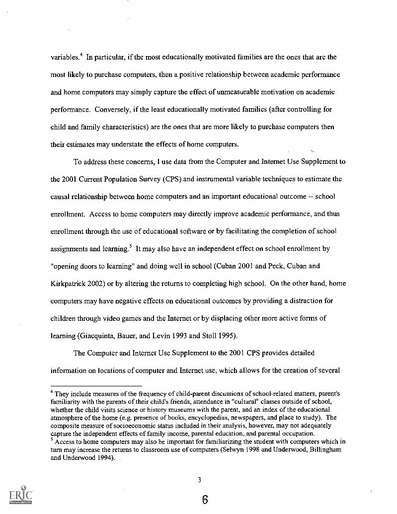
variables.4 In particular, if the most educationally motivated families are the ones that are the

most likely to purchase computers, then a positive relationship between academic performance

and home computers may simply capture the effect of unmeasurable motivation on academic

performance. Conversely, if the least educationally motivated families (after controlling for

child and family characteristics) are the ones that are more likely to purchase computers then

their estimates may understate the effects of home computers.

To address these concerns, I use data from the Computer and Internet Use Supplement to

the 2001 Current Population Survey (CPS) and instrumental variable techniques to estimate the

causal relationship between home computers and an important educational outcome school

enrollment. Access to home computers may directly improve academic performance, and thus

enrollment through the use of educational software or by facilitating the completion of school

assignments and learning.5 It may also have an independent effect on school enrollment by

"opening doors to learning" and doing well in school (Cuban 2001 and Peck, Cuban and

Kirkpatrick 2002) or by altering the returns to completing high school. On the other hand, home

computers may have negative effects on educational outcomes by providing a distraction for

children through video games and the Internet or by displacing other more active forms of

learning (Giacquinta, Bauer, and Levin 1993 and Stoll 1995).

The Computer and Internet Use Supplement to the 2001 CPS provides detailed

information on locations of computer and Internet use, which allows for the creation of several

4 They include measures of the frequency of child-parent discussions of school-related matters, parent'sfamiliarity with the parents of their child's friends, attendance in "cultural" classes outside of school,whether the child visits science or history museums with the parent, and an index of the educationalatmosphere of the home (e.g. presence of books, encyclopedias, newspapers, and place to study). Thecomposite measure of socioeconomic status included in their analysis, however, may not adequatelycapture the independent effects of family income, parental education, and parental occupation.5 Access to home computers may also be important for familiarizing the student with computers which inturn may increase the returns to classroom use of computers (Selwyn 1998 and Underwood, Billinghamand Underwood 1994).

3

6

instrumental variables for computer ownership. Computer and Internet use at work by the child's

parents should affect the probability of the family purchasing a home computer, but should not

affect academic performance (after controlling for other factors). 6 There exists a strong

correlation between using a computer at work by a household member and computer ownership

by that household (U.S. Department of Commerce 2002). In addition, there is no obvious reason

why we would expect parental use of computers or the Internet at work to have a strong effect on

educational outcomes after controlling for family income, and the education levels and

occupations of the child's parents. I provide evidence on these issues below.

II. Data

I use data from the Computer and Internet Usage Supplement to the September 2001

Current Population Survey (CPS). The survey, conducted by the U.S. Census Bureau and the

Bureau of Labor Statistics, is representative of the entire U.S. population and interviews

approximately 50,000 households. It contains a wealth of information on computer and Internet

use, including detailed data on types and location of use.

The main sample used in the following analysis includes only children ages 16-18 who

have not graduated from high school and live with at least one parent.' Parents living in the

same household as the child are identified by using parent and spouse identification numbers

provided by the CPS. Using this information, however, I cannot distinguish between biological

parents and stepparents.

6 Similar instruments -- the non-home use of the Internet by various household members -- have beenused in Kuhn and Skuterod's (2001) study of the effects of on-line job search on unemployment spells.7 Of the total sample, 93.3 percent live with at least one parent.

4

HI. Computer and Internet Use

The presence of computers and the Internet in the nation's schools is ubiquitous. The

National Center for Education Statistics reported that 100 percent of all public secondary schools

in the fall of 2001 were connected to the Internet (U.S. Department of Education, 2001b). In

these schools, 88 percent of all instructional classrooms had Internet access, and there were 0.23

instructional computers per student on average.

For the sample of high school students ages 16-18 from the 2001 CPS, reported rates of

computer and Internet use reflect these high levels of access. Ninety percent of enrolled high

school students report using a computer at school and 62 percent report using the Internet at

school.

Access to computers and the Internet at home is not universal, but fairly high. Slightly

less than 77 percent of children ages 16 to 18 who have not graduated from high school and live

with at least one parent have access to a computer at home (see Table 1). Levels of access,

however, vary tremendously across income, educational and racial groups (see U.S. Department

of Commerce 2002 and Fairlie 2002).

Patterns of home computer use are revealing. Teenagers appear to be using their home

computers -- 94.6 percent of children who have access to a home computer use it. Interestingly,

95.0 percent of children who are enrolled in school use their home computer compared to 87.1

percent of children who are not enrolled in school suggesting that computers may be useful for

completing homework assignments. Examining this issue directly, estimates from the CPS

indicate that of those children who use a home computer and are currently enrolled in school,

92.8 percent use their computer to complete school assignments.

5

Teenagers also use home computers for many other purposes. The most common uses of

home computers among teenagers are for the Internet (88.0 percent), games (81.5 percent), email

(80.9 percent), and word processing (72.2 percent). Use of home computers for graphics and

design (32.5 percent) and spreadsheets or databases (25.0 percent) are also fairly common. None

of these uses among high school students, however, is as prevalent as using home computers to

complete school assignments. Furthermore, the large percentage of high school students,

especially relative to the percentage of dropouts, using home computers for word processing

provides additional evidence that home computers are useful for completing homework

assignments. Concerns that home computers are only used for non-educational purposes such as

playing games, listening to music, and emailing friends, seem exaggerated (Giacquinta, Bauer

and Levin 1993).

The Internet also appears to be useful for schoolwork. Nearly 90 percent of high school

students who use the Internet use it to complete school assignments (see Table 2).8 Perhaps this

is not surprising given the proliferation of homework help sites on the web and high rates of

access in schools (Lenhart, Simon, and Graziano 2001). The Internet is also frequently used,

however, for non-educational purposes such as playing games (58.3 percent), chat rooms (37.0

percent), viewing TV or movies or listening to music (27.3 percent), and shopping (22.5

percent).

At a minimum, estimates from the 2001 CPS indicate that home computers and the

Internet are useful for completing school assignments. Whether these students wrote better

reports or could have completed their school assignments at a library, community center or

school, however, is unknown. Furthermore, the prevalence of non-educational uses of

8 The CPS does not distinguish between Internet use at home, school or other locations.

6

9

information technology, such as games, chat rooms and music, suggests that home computers

may also provide a distraction that lessens or negates their educational impact.

IV. The Effects of Home Computers on School Enrollment

School enrollment among teenagers is positively associated with owning a home

computer. Table 3 reports estimates of enrollment rates among children ages 16-18 who have

not finished high school by access to home computers. Slightly more than 95 percent of children

with home computers are enrolled in school. In comparison, only 85.4 percent of children

without access to home computers are enrolled in school.9 Although these estimates do not

control for factors, such as the child's age or his/her family's income, they are suggestive of the

direction and size of potential impacts.

To control for these factors and others, I first model the school enrollment decision.

Assume that school enrollment is determined by an unobserved latent variable,

(4.1) Yi* = X, 'fi + C,'8+ ui,

for person i, i=1,....,N. Only Y, is observed, which equals 1 if Y,* 0, implying that person i

chooses to enroll in school; Y,* equals zero otherwise. Xi is a vector of individual, family and

geographical area characteristics, C, is a dummy variable for the presence of a home computer,

and u, is the error term. Assuming that u, is normally distributed, the data are described by the

following probit model.

(4.2) Prob(Y,=1) = 0(Xi'fl + C/8),

9 Attewell and Battle (1999) also find large differences in academic performance based on access to homecomputers using the NELS. In particular, they find than eighth graders with home computers scored 6points higher on reading and 5 points higher on math that eighth graders without home computers(average scores among NELS respondents on both tests were approximately 50).

7

10

where 0 is the cumulative normal distribution function. Although the normality assumption

should only be taken as an approximation, the probit model provides a useful descriptive model

for the binary event that a child enrolls in school.

Table 4 reports estimates from probit regressions for the probability of school enrollment

among children ages 16 to 18 who have not graduated from high school. All specifications

include the sex, race, and age of the child, number of children in the household, family income,

mother's and father's presence in the household, education level, labor force status and

occupation, region of the country, central city status, and the state-level unemployment rate,

pupil-teacher ratio, average expenditures per pupil and dummy variables for the age

requirements of compulsory schooling laws (means for most variables are reported in the

Appendix).1° As expected, family income and parental education have large positive effects on

school attendance. Older children and boys have lower probabilities of attending school, all else

equal.

Owning a home computer appears to increase the probability of high school enrollment.

The coefficient estimate on the home computer variable is large, positive, and statistically

significant. The marginal effect evaluated at the mean characteristics of the sample, which is

reported below the coefficient estimate, implies that having a home computer is associated with a

0.0138 higher probability of being enrolled in school." The effect of this variable on the

probability of school enrollment is comparable in size to that implied by being a girl and is

slightly smaller thap that implied by having a high-school- or "some college-" educated mother

(relative to a high school dropout). The effect, however, is much smaller than that implied by

10 The state-level unemployment rate is from Bureau of Labor Statistics (2002), and the age requirementsfor compulsory schooling laws, pupil-teacher ratio and average expenditures per pupil are from U.S.Department of Education (2001a)." The average treatment effect, which equals 1/n E (1)(X,1(3 + 8) - (D(Xii(3), is larger (0.0195).

8

11

being 18 years old (relative to 16), having a college-educated mother, or moving from the bottom

of the family income distribution to the top.

An immediate concern with these estimates is that some families may have purchased

their computers after or near the time that the school enrollment decision was made, and thus

may be caused directly by the school enrollment decision. Although the CPS does not provide

information on the timing of when all computer purchases were made, it provides information on

when the newest computer was obtained by the family. Therefore, as a check of these results I

estimate a probit model that excludes all observations for which the newest computer was

obtained in 2001. This exclusion is likely to be overrestrictive, however, because a computer

purchased in 2001 may represent a replacement for an older model or may have been purchased

several months prior to the survey date, which is in September. The results are reported in

Specification 2 of Table 4. The coefficient estimate on home computer is slightly larger in this

specification.

The findings from the probit model for school enrollment are consistent with the findings

from previous research on the relationship between home computers and other educational

outcomes using the 1988 National Educational Longitudinal Survey. Attewell and Battle (1999)

provide evidence that test scores and grades are positively related to home computer use. As

noted above, even after controlling for differences in several demographic and individual

characteristics, students with home computers were found to score 3 to 5 percent higher than

students without home computers.

BIVARIATE PROBIT RESULTS

Although the findings presented in Attewell and Battle (1999) and those presented above

are based on regression models that include numerous controls for individual, parental, and

family characteristics, estimates of the effects of home computers on educational outcomes may

be biased. For example, if children with higher levels of academic ability or children with more

"educationally motivated" parents are more likely to have access to home computers, then the

probit estimates may overstate the effect of home computers on school attendance. On the other

hand, if parents of children with less academic ability or time to spend with their children are

more likely to purchase computers, then the probit estimates may understate the effect. In either

case, the effects of unobserved factors, such as academic ability and parental motivation, may

invalidate the causal interpretation of the previous results.

A potential solution to this problem is to estimate a bivariate probit model in which

equations for the probability of school enrollment and the probability of having a home computer

are simultaneously estimated. This model is equivalent to an instrumental variables or two-stage

least squares model and is preferred when both the dependent variable and endogenous variable

are binary.

Similar to (4.1), assume that home computer ownership is determined by an unobserved

latent variable,

(4.3) C,* = .A1,1y+ + e,,

where only C, equal to 0 or 1 is observed, Z, is a vector of variables that are not included in (4.1),

and si is the error term. In this case, u, and ei are distributed as bivariate normal with mean zero,

unit variance, and p=Corr(ub ed. The bivariate probit model is appropriate when p960.

The choice of Z, is of paramount importance. I use information on whether the child's

mother and father use a computer and the Internet at work. Computer and Internet use at work

by the child's parents should satisfy the two necessary properties of a valid instrumental variable

-- they affect the probability of purchasing a computer, but do not affect academic performance

(after controlling for other factors). There exists a strong correlation between using a computer

at work by a household member and computer ownership by that household (U.S. Department of

Commerce 2002). In addition, we do not expect the use of a computer at work by the child's

mother or father to have a strong effect on educational outcomes after controlling for family

income, parental education, and parental occupations. Computer use at work may be associated

with higher earnings, but this effect should be controlled for by the inclusion of family income.

Similar instruments have been used to examine the effects of on-line job search on

unemployment durations (Kuhn and Skuterod 2001). Specifically, the non-home use of the

Internet by various household members is used as an instrument for on-line job search. Kuhn

and Skuterod argue that these instruments, especially the non-home use of the Internet by a

household member outside one's nuclear family, should affect Internet use for job search by an

unemployed respondent, but should not directly affect the length of the respondent's

unemployment spell.

Estimates from the bivariate probit model for the probability of school attendance and

having a home computer are reported in Specification 3 of Table 4. As expected, parental

education is an important determinant of owning a home computer (reported in the first column).

The probability of owning a home computer generally increases with both mother's and father's

education. Education may be a proxy for wealth or permanent income and have an effect on the

budget constraint or may have an effect on preferences for computers through pure tastes,

11

i4

exposure, perceived usefulness, or conspicuous consumption. Family income is also important

in determining who owns a home computer. The relationship between the home computer

probability and income is almost monotonically increasing across the listed categories. It is

likely to be primarily due to its effect on the budget constraint, however, it may also be due its

effect on preferences.

Race and ethnicity are also important determinants of computer ownership. Black,

Latino, and Native American children have lower probabilities of having a home computer than

do white children. In addition to these control variables, age, number of children, and region

also have statistically significant effects on the home computer probability.

All four instrumental variables have positive coefficients in the home computer equation.

Only mother's use of the Internet at work and father's use of the Internet at work, however, are

statistically significant at conventional levels. The coefficients on these variables imply large

effects on the probability of having a home computer. In particular, if the father uses the Internet

at work then the probability of having a home computer is 0.0811 higher, all else equal. The

stronger effects of Internet use compared to computer use at work may imply that

communication and information retrieval uses of computers at work are associated with

purchasing home computers and not other uses, such as appointment scheduling, database entry,

and production.

The second column in Specification 3 reports the bivariate probit results for the school

enrollment equation. Having a home computer has a large, positive and statistically significant

effect on school enrollment. The coefficient estimate implies that the presence of a home

computer increases the probability of school enrollment among children by 0.0767.12 This effect

is quite large as the sample average for the probability of school enrollment is 0.936.

12 The average treatment effect is 0.1173.

12

15

Interestingly, this estimate lies between the probit estimate (0.0138) and the raw difference in

school enrollment rates between children who have access to home computers and those who do

not (0.098). Related to this issue the estimate of p indicates a negative correlation between the

unobserved factors affecting home computers and school enrollment. Although it is unclear

what causes this relationship, one possibility is that the least "educationally-motivated" families

after controlling for observables are the ones that are most likely to purchase computers perhaps

motivated by the many recreational uses of computers.

Why might we expect that access to home computers will have a positive effect on school

enrollment among teenagers? There are several reasons. First, computers may improve

academic performance directly through the use of educational software. Second, home

computers may facilitate the completion of school assignments and learning either by making

it easier and more rewarding to complete homework assignments or by familiarizing the student

with computers increasing the returns to computer use in the classroom (Underwood, Billingham

and Underwood 1994). Estimates reported above indicate that approximately 9 out of 10 high

school students who have access to a home computer use that computer to complete school

assignments, and 46 percent of teachers report that student access to technology/Internet is a

barrier to effective use of technology in the classroom (SRI 2002). Third, the use of computers

may "open doors to learning" and doing well in school (Cuban 2001 and Peck, Cuban and

Kirkpatrick 2002), and thus may encourage some teenagers to stay in schoo1.13 Finally, home

computers and the skills acquired using them may alter the economic returns to completing high

school. For example, computer skills may be improve employment opportunities, but only after

meeting the minimum threshold of graduating from high school.

13 The use of computers at home may also translate into more positive attitudes towards informationtechnology potentially leading to long-term use (Selwyn 1998). Many teachers report that educationaltechnology increases outside class time initiative among students (SRI 2002).

13

16

INSTRUMENTAL VARIABLE ISSUES

The evidence from the bivariate probit model suggests that access to home computers

increase the likelihood of staying in school. As noted above, this interpretation depends on

whether work computer and Internet use by parents satisfy the two necessary properties of valid

instrumental variables they are partially correlated with the home computer probability (after

netting out X1), but are not correlated with the school enrollment probability (i.e. uncorrelated

with 10. Internet use at work by the child's mother and father, at least, appear to be consistent

with the first requirement. The coefficient estimates in the home computer equation are positive

and statistically significant. The coefficient estimates, however, on the mother's and father's

computer use at work variables are not statistically significant in the bivariate probit mode1.14

Because of concerns about the effects of weekly correlated instruments (e.g. Bound,

Jaeger, and Baker 1995 and Staiger and Stock 1997), I estimate a bivariate model that only

includes mother's and father's use of the Internet at work as instrumental variables. I am also

concerned about the interdependence of the instruments. Of those mothers and fathers who use a

computer at work, 65.5 and 77.3 percent also use the Internet at work, respectively. Estimates

are reported in Specification 1 of Table 5. The coefficient estimate on having a home computer

is slightly larger and remains statistically significant. As expected, the implied effects of

mother's and father's use of the Internet at work on having a home computer are now larger and

more significant.

I also estimate a model that only includes a dummy variable for whether either parent

uses the Internet at work (Specification 2). Approximately, 40 percent of children who have one

14 The coefficient estimates and statistical significance for the instruments are very similar in a probitmodel for the probability of having a home computer.

14

parent who uses the Internet at work also have another parent who uses the Internet at work. The

coefficient estimate on home computer is slightly larger than the estimate in the main

specification. Another test of the sensitivity of results is to estimate the probit model only

including the computer at work instruments. The results are reported in Specifications 3 and 4.

In both cases, the coefficient estimates are similar to the original estimates. The coefficients on

mother's and father's use of computers at work are now statistically significant. The estimates

reported in Table 5 indicate that the estimated effect of home computers on school enrollment is

quite robust to alternative specifications of instruments, such as the exclusion of "weaker"

instruments or correlated instruments.

Are computer and Internet use at work by the child's parents uncorrelated with u,? One

method of exploring this issue is to estimate a probit model for school enrollment that includes

the four instrumental variables. Although not reported, I find that none of the instruments is

statistically significant. Mother's and father's use of computers at work have negative

coefficients, and mother's and father's use of the Internet at work have positive coefficients. I

also estimate probit models for school enrollment that include all four combinations of

instruments listed in Table 5. In each of the specifications, none of the instruments has a

statistically significant coefficient estimate. Although this is not a formal test of the validity of

the instruments, it suggests that computer and Internet use at work by the child's parents do not

have a large effect on the probability of being enrolled in school after controlling for family

income, parental education, parental occupation, and other factors.

15

I8

ADDITIONAL ESTIMATES

I investigate the sensitivity of the results to several alternative samples. First, similar to

above, I estimate a specification that excludes all children living in households in which the

newest computer was obtained in 2001. The exclusion of these children rules out the possibility

that some families may have purchased their computers after or near the time that the school

enrollment decision was made. Specification 1 of Table 6 reports results. The coefficient

estimate implies a slightly larger effect and remains statistically significant.

Another concern regarding the robustness of estimates is the exclusion of children who

do not live with their parents. The main justification for removing these children is that they do

not have parents who are "at risk" of using a computer and/or the Internet at work for use as

instrumental variables. One method of addressing this concern is to add these children back to

the sample and set mother's and father's use of computers and the Internet at work to zero.

Estimates are reported in Specification 2. The coefficient estimate for home computer is not

sensitive to the inclusion of these children.

The age requirements for compulsory schooling laws differ across states ranging from 16

to 18 (U.S. Department of Education 2001a). I currently include dummy variables for whether

the age requirements are 17 or 18 years of age (with age 16 being the left out category).

However, I am concerned that the process determining school enrollment may differ between

children under the age cutoff and children above the age cutoff.15 To address this issue, I

estimate a bivariate probit model that excludes all children under the age requirement of the

compulsory schooling law in their state. Estimates are reported in Specification 3. The

coefficient estimate implies a similar size effect although it is no longer statistically significant.

15 School enrollment rates are not 100 percent for children who are younger than the age requirement forcompulsory schooling in their state. For example, less than 97 percent of 17-year olds living in stateswith age 18 compulsory schooling laws are enrolled in school.

16

In all previous specifications I include a dummy variable for missing family income,

which represents 14.0 percent of the sample. Specification 4 reports estimates for a sample that

excludes these missing values. The coefficient estimate is not sensitive to this change. Finally, I

experimented with specifications that alternately removed the controls for parental occupation,

parental education, and state-level variables. The coefficient on the home computer variable was

not sensitive to any of these changes. Overall, the coefficient estimate on home computer in the

bivariate probit is quite robust to alternative specifications and samples.

V. Conclusions

Estimates from the Computer and Internet Use Supplement to the 2001 Current

Population Survey, provide evidence on whether access to home computers increases the

likelihood of school enrollment among teenagers who have not graduated from high school. A

comparison of school enrollment rates reveals that 95.2 percent of children who have home

computers are enrolled in school, whereas only 85.4 percent of children who do not have home

computers are enrolled in school. I find a smaller, but large positive difference in school

enrollment rates after estimating a bivariate probit model for the joint probability of school

enrollment and owning a home computer. Use of computers and the Internet at work by the

child's mother and father are used as instrumental variables. The coefficient estimates imply that

the probability of school enrollment is 0.0767 higher in the presence of a home computer. I

interpret the results as providing evidence that home computers increase the likelihood of being

enrolled in school.

Although the results are exceptionally robust to alternative specifications and samples,

there is always the possibility that the large positive estimates of the effect of home computers on

17

school enrollment are due to a correlation between the instruments and the error term in the

enrollment equation. One potential problem is that parents with Internet access at work may be

more able to communicate via email with teachers regarding their child's academic, attendance or

behavior problems in school resulting in better educational outcomes. Only 28 percent of

parents, however, report using email to communicate with their children's teachers (Lenhart,

Simon, and Graziano 2001). Furthermore, the majority of email communication between parents

and teachers may occur at home instead of work.

Unfortunately, the CPS does not include information on other aspects of work (e.g. the

use of pencils) that would allow for a "reality check" of the results using computer or Internet use

at work as instruments for home computers. In the end, however, there is no obvious reason to

suspect that parental use of computers or the Internet at work is strongly correlated with

educational outcomes after controlling for family income, and the education levels and

occupations of the child's parents. Although more research is needed, the estimates presented

above suggest that the household consumption of computers may provide positive externalities to

families through better educational outcomes among children.

References

Angrist, Joshua, and Victor Lavy. 1999. "New Evidence on Classroom Computers and PupilLearning," National Bureau of Economic Research Working Paper No. 7424.

Attewell, Paul, and Juan Battle. 1999. "Home Computers and School Performance," TheInformation Society, 15: 1-10.

Autor, David H. 2001. "Wiring the Labor Market." Journal of Economic Perspectives. 15: 1, 25-40.

Bakos, Yannis. 2001. "The Emerging Landscape for Retail E-Commerce." Journal of EconomicPerspectives. 15: 1, 69-80.

Borenstein, Severin, and Garh Saloner. 2001. "Economics and Electronic Commerce." Journal ofEconomic Perspectives. 15: 1, 3-12.

Bound, John, David A. Jaeger, and Regina Baker. 1995. "Problems with Instrumental VariablesEstimation when the Correlation between the Instruments and the Endogenous ExplanatoryVariables Is Weak?" Journal of the American Statistical Association, 90: 430, 443-450.

Bureau of Labor Statistics. 2002. State and Regional Unemployment, 2001 Annual Averages.ftp://ftp.b1s.gov/pub/news.release/srgune.txt.

Crandall, Robert W. 2000. "Bridging the Digital Divide: Universal Service, Equal Access, andthe Digital Divide," paper presented at Bridging the Digital Divide: California Public AffairsForum, Stanford University.

Cuban, Larry. 2001. Oversold and Underused: Computers in the Classroom. Cambridge: HarvardUniversity Press.

Fair lie, Robert W. 2002. "Race and the Digital Divide," Joint Center for Poverty ResearchWorking Paper No. 307.

Federal Communications Commission. 2000. "In the Matter of Inquiry Concerning theDeployment of Advanced Telecommunications Capability to All Americans in a Reasonable andTimely Fashion, and Possible Steps to Accelerate Such Deployment Pursuant to Section 706 ofthe Telecommunications Act of 1996." CC Docket No. 98-146, Second Report, FCC 00-290.

Freeman, Richard B. 2002. "The Labour Market in the New Information Economy," NationalBureau of Economic Research Working Paper No. 9254.

Giacquinta, Joseph, JoAnne Bauer, and Jane Levin. 1993. Beyond Technology's Promise: AnExamination of Children's Educational Computing at Home. New York: Cambridge UniversityPress.

19

Kawaguchi, Daiji. 2001. "Are Computers at Home a Form of Consumption or Investment? ALongitudinal Analysis for Japan," Michigan State University Working Paper.

Kirpatrick, H., and L. Cuban. 1998. "Computers Make Kids Smarter--Right?" Technos Quarterlyfor Education and Technology, 7:2.

Krueger, Alan B. 1993. "How Computers Have Changed the Wage Structure: Evidence fromMicro Data." The Quarterly Journal of Economics. 107:1, 35-78.

Kuhn, Peter, and Mikal Skuterud. 2001. "Does Internet Job Search Reduce UnemployedWorkers' Jobless Durations?" University of California, Santa Barbara, Working Paper.

Kuhn, Peter, and Mikal Skuterud. 2000. "Job Search Methods: Internet versus Traditional."Monthly Labor Review, October, pp. 3-11.

Lenhart, Amanda, Maya Simon, and Mike Graziano. 2001. "The Internet and Education:Findings from the Pew Internet & American Life Project," Washington, D.C.: Pew Internet &American Life Project.

Morton, Fiona Scott, Florian Zettelmeyer, and Jorge Siva Risso. 2000. "Internet Car Retailing."Yale University Working Paper.

Noll, Roger G. Noll, Dina Older-Aguilar, Gregory L. Rosston, and Richard R. Ross. 2000. "TheDigital Divide: Definitions, Measurement, and Policy Issues," paper presented at Bridging theDigital Divide: California Public Affairs Forum, Stanford University.

Peck, Craig, Larry Cuban, and Heather Kirkpatrick. 2002. "Techno-Promoter Dreams, StudentRealities," Phi Delta Kappan. 83:6, 472-80.

Puma, Michael J., Duncan D. Chaplin, and Andreas D. Pape. 2000. E-Rate and the DigitalDivide: A Preliminary Analysis from the Integrated Studies of Educational Technology. UrbanInstitute.

Ratchford, Brian T., Debabrata Talukdar, and Myung-Soo Lee. 2001. "A Model of ConsumerChoice of the Internet as an Information Source." International Journal of Electronic Commerce.5: 3, 7-21.

Selwyn, Neil. 1998. "The Effect of Using a Home Computer on Students' Educational Use ofIT," Computers and Education, 31: 211-227.

Servon, Lisa. 2002. Bridging the Digital Divide: Community, Technology and Policy(Blackwell).

SRI International. 2002. The Integrated Studies of Educational Technology: ProfessionalDevelopment and Teachers' Use of Technology," SRI International Report.

20

Staiger, Douglas, and James H. Stock. 1997. "Instrumental Variables Regression with WeakInstruments," Econometrica, 65: 3, 557-586.

Stoll, Clifford. 1995. Silicon Snake Oil: Second Thoughts on the Information Highway. NewYork: Doubleday.

Underwood, J., Billingham. M. and Underwood, G. 1994. "Predicting Computer Literacy: HowDo the Technological Experiences of Schoolchildren Predict Their Computer Based Problem-Solving Skills? Journal of Information Technology for Teacher Education, 3(1), 115-125.

U.S. Department of Commerce. 2002. A Nation Online: How Americans are Expanding TheirUse of the Internet. Washington, D.C.: U.S.G.P.O.

U.S. Department of Education. 2001. Digest of Educational Statistics 2001. Washington, D.C.:National Center for Educational Statistics.

U.S. Department of Education. 2001. Internet Access in U.S. Public Schools and Classrooms:1994-2000. Washington, D.C.: National Center for Educational Statistics.

U.S. Department of Labor 2000, Occupational Outlook Handbook, Washington, D.C.:U.S.G.P.O.

21

24

Table 1Home Computer Use among Children Ages 16-18

Current Population Survey, 2001

Enrolled inAll Children School Not Enrolled

Percent of children with access to a 76.6% 78.5% 52.1%home computerSample size

Percent of children with access to ahome computer who use that computerSample size

Percent of home computer users who:

use computer for school assignments

use computer for the Internet

use computer for games

use computer for electronic mail

use computer for word processing

use computer for graphics and design

use computer for spreadsheets ordatabases

Sample sizeNotes: (1) The sample consists of children ages 16-18 who have not graduated from highschool and live with at least one parent. (2) All estimates are calculated using sampleweights provided by the CPS.

4281

94.6%

4008

95.0%

273

87.1%

3370 3217 153

92.8%

88.0% 88.5% 78.5%

81.5% 81.5% 82.8%

80.9% 81.5% 67.4%

72.2% 73.6% 43.5%

32.5% 32.8% 24.2%

25.0% 25.0% 25.4%

3189 3056 133

Table 2Internet Use among Children Ages 16-18

Current Population Survey, 2001

All ChildrenEnrolled in

School Not EnrolledPercent of children who use the Internetanywhere

77.9% 80.1% 49.2%

Sample size 4281 4008 273

Percent of Internet users who:

use the Internet to completeschool assignments

use the Internet for electronic mail 83.7%

89.2%

84.0% 78.0%

use the Internet for playing games 58.3% 58.0% 65.6%

use the Internet to search for informationabout products and services

use the Internet to get news, weatheror sports

use the Internet for chat roomsor LISTSERVs

use the Internet for viewing TV ormovies, or listening to music

use the Internet to purchaseproducts or services

54.0%

53.3%

37.0%

27.3%

22.5%

54.2%

53.3%

36.5%

27.2%

22.5%

50.3%

52.6%

46.8%

28.8%

22.8%

Sample size 3433 3298 135Notes: (1) The sample consists of children ages 16-18 who have not graduated from highschool and live with at least one parent. (2) All estimates are calculated using sampleweights provided by the CPS.

Table 3School Enrollment. among Children Ages 16-18

Current Population Survey, 2001

Enrollment Sample SizeRate

School enrollment among childrenwithout access to home computer

School enrollment among children withaccess to home computer

85.4% 911

95.2% 3370

Notes: (1) The sample consists of children ages 16-18 who have notgraduated from high school and live with at least one parent. (2) Allestimates are calculated using sample weights provided by the CPS.

Table 4Probit and Bivariate Probit Regressions for School Enrollment and Home Computer

Current Population Survey, 2001

SpecificationExplanatory Variables (1) (2) (3)Dependent variable Enrollment Enrollment Computer EnrollmentModel type Probit Probit Bivariate BivariateFemale 0.1975 0.1797 0.0941 0.1819

(0.0709) (0.0750) (0.0541) (0.0780)

Black 0.2062 0.1945 -0.6869 0.3501(0.1179) (0.1232) (0.0842) (0.1399)

Latino 0.0364 0.0006 -0.4218 0.1320(0.1233) (0.1291) (0.0882) (0.1429)

Native American 0.1593 0.3016 -0.6420 0.2941(0.2397) (0.2664) (0.1830) (0.2944)

Asian 0.3489 0.4850 0.1748 0.3130(0.2443) (0.2890) (0.1474) (0.2808)

Age 17 -0.3067 -0.3107 -0.0493 -0.2963(0.0873) (0.0930) (0.0589) (0.1016)

Age 18 -1.3409 -1.3088 -0.2435 -1.2604(0.0904) (0.0958) (0.0780) (0.1113)

Family income: missing 0.2490 0.2891 0.3419 0.1376(0.1643) (0.1711) (0.1261) (0.1826)

Family income: $10,000 to 0.0171 0.0052 0.1218 -0.0070$15,000 (0.1825) (0.1887) (0.1469) (0.1933)

Family income: $15,000 to 0.0841 0.1519 0.3185 -0.0030$20,000 (0.2036) (0.2149) (0.1541) (0.2082)

Family income: $20,000 to 0.1071 0.2128 0.1514 0.0565$25,000 (0.1811) (0.1904) (0.1406) (0.1921)

Family income: $25,000 to 0.0891 0.0413 0.3772 -0.0127$30,000 (0.1921) (0.1982) (0.1453) (0.2063)

Family income: $30,000 to 0.0401 0.1586 0.4234 -0.0721

$35,000 (0.1947) (0.2078) (0.1549) (0.2173)

Family income: $35,000 to 0.1737 0.1649 0.6257 0.0168$40,000 (0.2115) (0.2214) (0.1631) (0.2334)

Family income: $40,000 to 0.3246 0.3282 0.6831 0.1327$50,000 (0.1818) (0.1896) (0.1402) (0.2258)

Family income: $50,000 to 0.1380 0.2582 0.7657 -0.0357$60,000 (0.1904) (0.2038) (0.1528) (0.2151)

(continued)

28

Probit and Bivariate Probit

Explanatory Variables

Table 4 (continued)Regressions for School Enrollment and Home Computer

Specification(1) (2) (3)

Family income: $60,000 to 0.4841 0.5443 0.8480 0.2890$75,000 (0.2042) (0.2187) (0.1542) (0.2334)

Family income more than 0.3810 0.3364 0.9684 0.1960$75,000 (0.1845) (0.1943) (0.1505) (0.2117)

Mother-high school graduate 0.2413 0.2855 0.2681 0.1584(0.1103) (0.1148) (0.0848) (0.1230)

Mother-some college 0.2529 0.2891 0.5511 0.1268(0.1224) (0.1283) (0.0949) (0.1480)

Mother-college graduate 0.4199 0.4342 0.5436 0.2984(0.1602) (0.1701) (0.1266) (0.1780)

Father-high school graduate -0.0134 -0.0940 0.0565 -0.0294(0.1278) (0.1361) (0.0922) (0.1352)

Father-some college 0.0150 -0.0186 0.1989 -0.0318(0.1406) (0.1509) (0.1047) (0.1489)

Father-college graduate 0.2428 0.2538 0.5248 0.1991(0.1775) (0.1953) (0.1453) (0.1879)

Home computer 0.1878 0.2115 0.8562(0.0864) (0.0904) (0.3152)

Marginal effect 0.0138 0.0166 0.0767Mother uses computer 0.0924

at work (0.0885)

Father uses computer 0.1433at work (0.1117)

Mother uses the Internet 0.2251

at work (0.0982)

Father uses the Internet 0.4034at work (0.1335)

Mother's occupation controls Yes Yes Yes YesFather's occupation controls Yes Yes Yes Yes

-0.3958(0.1790)

Mean of dependent variable 0.9358 0.9321 0.7860 0.9358Sample size 4,239 3,607 4,239Notes: (1) The sample consists of youth ages 16-18 who have not graduated from high schooland live with at least one parent. (2) The sample in Specification 2 excludes children in familiesobtaining their newest home computer in 2001. (3) All equations also include a constant,number of children in the household, dummy variables for region, central city status, mother'sand father's presence in the household and labor force status, and the state-levelunemployment rate, pupil-teacher ratio, average expenditures per pupil, and dummy variablesfor the age requirements of compulsory schooling laws.

Table 5Additional Bivariate Probit Regressions Using Different Instruments

Current Population Survey, 2001

Specification(1) (2) (3) (4)

Home computer 0.9014 0.9509 0.8029 0.8655(0.3051) (0.2966) (0.3380) (0.3224)

Marginal effect 0.0820 0.0881 0.0710 0.0783

Instrumental variables

Mother uses the Internet 0.2783at work (0.0846)

Father uses the Internet 0.5103at work (0.1005)

Either parent uses the Internet 0.4879at work (0.0730)

Mother uses computer 0.2132at work (0.0757)

Father uses computer 0.3794at work (0.0838)

Either parent uses computer 0.3311

at work (0.0674)

-0.4212 -0.4506 -0.3638 -0.3994(0.1713) (0.1666) (0.1952) (0.1849)

Mean of dependent variable 0.9358 0.9358 0.9358 0.9358Sample size 4,239 4,239 4,239 4,239Note: See notes to Table 4.

30

Table 6Additional Bivariate Probit Regressions Using Various Samples

Current Population Survey, 2001

Specification(1) (2) (3) (4)

Sample restrictions Removes Adds Compulsory Removescomputers children schooling missing

purchased in2001

living alone sample incomeobservations

Home computer 1.1198 0.9958 0.7088 0.8868(0.2630) (0.2637) (0.4291) (0.3467)

Marginal effect 0.1214 0.1060 0.0740 0.0774

-0.5341 -0.4484 -0.2677 -0.3991(0.1451) (0.1526) (0.2539) (0.1947)

Mean of dependent variable 0.9321 0.9213 0.9147 0.9363Sample size 3,607 4,548 2,720 3,644Notes: (1) See notes to Table 4. (2) See text for a more detailed description of the samplerestrictions used in each specification.

AppendixSample Means of Selected Variables

Current Population Survey, 2001

Variable MeanStandardDeviation

School enrollment 0.9358 0.2451

Home computer 0.7860 0.4102

Female 0.4735 0.4994

Black 0.1151 0.3192

Latino 0.0979 0.2972

Native American 0.0198 0.1394

Asian 0.0373 0.1895

Age 17 0.4084 0.4916

Age 18 0.1314 0.3379

Number of children in household 2.1515 1.2240

Family income: missing 0.1404 0.3474

Family income: $10,000 to $15,000 0.0422 0.2011

Family income: $15,000 to $20,000 0.0342 0.1818

Family income: $20,000 to $25,000 0.0533 0.2247

Family income: $25,000 to $30,000 0.0465 0.2105

Family income: $30,000 to $35,000 0.0495 0.2170

Family income: $35,000 to $40,000 0.0429 0.2027

Family income: $40,000 to $50,000 0.0937 0.2914

Family income: $50,000 to $60,000 0.0896 0.2857

Family income: $60,000 to $75,000 0.1064 0.3084

Family income more than $75,000 0.2574 0.4372

Lives only with father 0.0559 0.2298

Mother-not in the labor force 0.1925 0.3943

Lives only with mother 0.2404 0.4274

Mother-high school graduate 0.3218 0.4672

Mother-some college 0.2880 0.4529

Mother-college graduate 0.2232 0.4164

Father-high school graduate 0.2406 0.4275

Father-some college 0.1984 0.3988

Father-college graduate 0.2241 0.4170

Father-not in the labor force 0.0446 0.2064

Mother uses computer at work 0.4343 0.4957

Father uses computer at work 0.3711 0.4832

Mother uses the Internet at work 0.2843 0.4511

Father uses the Internet at work 0.2869 0.4523Sample size 4,239Note: The sample is the same as that used in Specification 3 of Table 4.

U.S. Department of EducationOffice of Educational Research and Improvement (OERI)

National Library of Education (NLE)Educational Resources Information Center (ERIC)

NOTICE

Reproduction Basis

fducelionol Resources Inforrootion Center

This document is covered by a signed "Reproduction Release (Blanket)"form (on file within the ERIC system), encompassing all or classes ofdocuments from its source organization and, therefore, does not require a"Specific Document" Release form.

This document is Federally-funded, or carries its own permission toreproduce, or is otherwise in the public domain and, therefore, may bereproduced by ERIC without a signed Reproduction Release form (either"Specific Document" or "Blanket").

EFF-089 (1/2003)