Munich Personal RePEc Archive

Renewable energy-economic growth

nexus in South Africa: Linear, nonlinear

or non-existent?

Nyoni, Bothwell and Phiri, Andrew

Nelson Mandela University

29 October 2018

Online at https://mpra.ub.uni-muenchen.de/89761/

MPRA Paper No. 89761, posted 30 Oct 2018 00:41 UTC

RENEWABLE ENERGY - ECONOMIC GROWTH NEXUS IN SOUTH

AFRICA: LINEAR, NONLINEAR OR NONEXISTENT?

Bothwell Nyoni

Innoventon and the Downstream Chemicals Technology Station, Nelson Mandela University,

South Africa, 6031.

And

Andrew Phiri

Department of Economics, Faculty of Business and Economic Studies, Nelson Mandela

University, Port Elizabeth, South Africa, 6031.

ABSTRACT: With escalating fears of climate change reaching irreversible levels, much

emphasis has been recently placed on shifting to renewable sources of energy in supporting

future economic livelihood. Focusing on South Africa, as Africa’s largest energy consumer

and producer, our study investigates the short-run and long-run effects of renewable energy on

economic growth using linear and nonlinear autoregressive distributive lag (ARDL) models.

Working with data availability, our empirical analysis is carried out over the period of 1991 to

2016, and our results unanimously fail to confirm any linear or nonlinear cointegration effects

of the consumption and production of renewable energy on South African economic growth.

We view the absence of cointergation relations as an indication of inefficient usage of

renewable energy in supporting sustainable growth in South Africa and hence advise

policymakers to accelerate the establishment of necessary renewable infrastructure in

supporting future energy requirements.

Keywords: Renewable energy; economic growth; ARDL; nonlinear ARDL; South Africa; Sub-

Sahara Africa (SSA).

JEL Classification Code: C13; C32; C52; Q43.

1 INTRODUCTION

In advancing its cause towards a globally cleaner energy environment, the International

Renewable Energy Agency (IRENA) has recently released “The Global Energy

Transformation: A Roadmap to 2050” (IRENA, 2015). The document mandates that

“…renewable energy needs to be scaled up to at least six times faster for the world to start to

meet the goals set out in the Paris [climate change] agreement…”. In order to reach these

targets, the report predicts that i) the total share of renewable energy must more than triple from

its current levels of 18 percent of total final energy consumption to around two-thirds or 67

percent by 2050, and ii) the share of renewables in the power sector are required to be boosted

from its current level of 25 percent to a four-fold increase of 85 percent. It is firmly believed

that such a transition towards a renewable energy dominated world will also accelerate global

progress towards the United Nations (UN) Sustainable Development Goal (SDP7) of providing

access to affordable, reliable, sustainable and modern energy for all people across the global.

However, for IRENA to attain these objectives, much investment expenditure in

corresponding infrastructure as well as technology is necessary, and it is predicted that the

global economy would have to sacrifice approximately 2 percent of global GDP per annum to

finance such developments. Despite such expected significant losses in future global GDP

growth being required for the transition towards increased usage of renewable energies, IRENA

predicts that economic benefits of investment in renewable energies outweigh their associated

economic costs. The document particularly projects an additional increase in global welfare by

15 percent, in GDP by 1 percent and in employment by 1 percent, in comparison to forecasts

derived from a reference case experiment where investment in such energy technologies were

not implemented. Another striking feature of the document is its particular reference to and

acknowledgement of the South African economy as the main representative country of the

African continent. With South African simultaneously standing as the largest producer of

energy as well as the largest emitter of carbon emissions in Africa, IRENA predicts that South

Africa will benefit through increased renewable energy usage via three main channels.

Firstly, increased reliance on renewable energy is expected to immensely decrease

South Africa’s greenhouse gas emissions, and this decrease in carbon emissions is expected to

be greater in comparison to that expected to be experienced by other countries or regions

globally. Secondly, it is believed that the transition towards cleaner energy usage is expected

to decrease South Africa’s imports of fossil fuels and consequentially increase consumption of

domestic goods and services. This, in turn, will assist in boosting the macroeconomy through

increased consumer expenditure and it’s resulting multiplier effects. Lastly, the combined

macroeconomic effect of the energy transition is expected to increase economic growth by 3

additional percent in comparison to baseline projections in which no such renewable energy

developments occur.

On the other end of the spectrum, the Renewable Energy Independent Power Producer

Procurement Programme (REIPPPP) initiated in 2011 by the South African Department of

Energy (DoE), serves as a blueprint for pursuing the renewable energy agenda orchestrated by

IRENA. The much celebrated REIPPPP document has been glorified as the world’s fastest

growing energy programme and one of the largest programmes in the current infrastructure

development portfolio for the South African economy. In particular, the REIPPPP programme

has been a dominant force in the global renewable energy markets in terms of ushering large-

scale development of energy generation infrastructure as well as providing a conducive

investment environment for energy infrastructure opportunities. However, contrary to the

optimism on the role of renewable energy in achieving improved economic development in

South Africa, very little empirical revelation has supported this cause. To put it more precise,

a majority of previous econometric analysis examining the effects of renewable energy on

economic growth in South Africa have found no significant effects amongst the time series (i.e.

Al-mulali et al. (2013), Tawari et al. (2015), Cho et al. (2015) and Bhattacharya et al. (2016)),

whilst a few others either find a positive short-run (Sebri and Ben-Salha (2014)) or long-run

(Apergis and Payne (2011) and Khobai and Le Roux (2018)) correlations between the

variables.

One avenue of empirical research which remains unscathed for the South African

economy or the entire sub-Saharan region as whole for that matter, relates to the issue of

possible asymmetries existing in the renewable energy-growth relationship. As recently

pointed out by Mbarek et al. (2018) the finding of a non-existent relationship between

renewable energy and economic growth may due to researchers dependency on linear

frameworks which are not be flexible enough to capture complex, asymmetric dynamics

between the variables. Consequentially, one way of circumventing this issue would be through

the use of nonlinear cointegration framework and up-to-date, very few studies have adopted

this empirical strategy with the existing literature exclusively focusing on non-Sub-Saharan

African economies (Apergis and Payne (2014), Apergis et al. (2016), Alper and Oguz (2016)

and Mbarek et al. (2018)). Our study contributes to this relatively fresh body of empirical

knowledge, by becoming the first to examine possible asymmetries in the renewable energy-

economic growth nexus for South Africa. In also differing from previous ‘nonlinear studies’,

we rely on the recently introduced nonlinear autoregressive distributive lag (N-ARDL) model

of Shin et al. (2014) which offers several advantages over other contending nonlinear

cointegration frameworks such as performing better in smaller sample sizes and the model’s

flexibility in establishing significant asymmetric cointegration relations amongst a

combination of I(0) or I(1) series.

The rest of the study is organized as follows. The following section provides a brief

overview of renewable energy developments in South Africa. The third section reviews the

associated literature review of the study. Section four presents the model and estimation

techniques and the empirical results are reported in section five. The study is then concluded

in the sixth section primarily in the form of policy implications.

2 BRIEF OVERVIEW OF RENEWABLE ENERGY DEVELOPMENTS IN

SOUTH AFRICA

South Africa is classified as a third world country with a total population of over 50

million people and, of the total population, 86% have access to electricity (Phiri and Nyoni,

2016). Eskom is the major supplier and distributor of energy through electricity production,

supplying up to 95% of the total electricity consumed, the other 5% comes from independent

power producers. Eskom has invested more than $22 billion since 2005 to increase its

generation, transmission and distribution capacity by building state of the art power plants,

expanding the transmission lines and at the same time decommissioning old inefficient power

plants which has opened up opportunities for Renewable Energy Independent Power Producers

(REIPP) (DEA, 2014; ESKOM, 2016). However, the current plans of building three new coal

power plants as means of increasing Eskom’s capacity of 44 087 to 52 589 MW, are of great

controversy, as electricity generation using coal fired power stations is the major green-house

gas (GHG) producing activity in the South African energy industry. Although the nation is

moving towards a renewable energy dominated energy matrix in reducing GHG emissions, it

is clear that the major source of electricity in the foreseeable future will still be coal. In line

with the global efforts to reduce fossil fuels consumption, the government of South Africa

unveiled vital policies that are expected to lead to the successful introduction of renewable

energy into the country’s electricity generation matrix. Of special interest from these policies

is the Renewable Energy White Paper of 2003 that stresses on formulating a strategy of

translating the renewable energy goals and objectives into practicality with wind, solar and

biomass being identified as sources with great potential of contributing more to the South

African electricity grid by 2025 (DOE, 2015).

The South African government’s commitment to renewable energy rollout has been

under scrutiny until a huge undertaking of obtaining approximately 18 GW of power from

renewable sources was suggested (Walwyn and Brent, 2015). From 1996 three main policies

were formulated, those being the White Paper on Energy Policy of 1998, White Paper on

Renewable Energy of 2003 and the National Climate Change Response White Paper Policy of

2011, but with unsatisfactory implementation (DOE, 2015). These policies were expected to

be implemented following the guidelines of an Integrated Resource Plan (IRP) for electricity

generation referred to as IRP 2010-2030. The objectives of the IRP 2010-2030 is to create a 20

year planning approach from 2010 to 2030 for the national utilities to meet the forecasted

energy demand of 89.5 GW by the year 2030 (DOE, 2013). The IRP 2010-2030 is supposed to

be updated and improved after every two years. The updated versions during the course of the

years have not been promulgated since 2010 making the original IRP to be used as a guideline

plan for the rolling out of energy development. The latest update at the preparation of this

manuscript came out in 2018 and it included a major reduction on the planned electricity from

nuclear sources. The newly updated IRP has the following electricity generation contributions;

8100 MW from wind; 8100 MW from gas; 5670 MW from solar photovoltaic; 2500 MW from

hydro and 1000 MW from coal (DOE, 2018). The updated IRP suggests that the planned

electricity generation from renewable sources will be 27%, a huge increase from the original

allocation of 21%. The major reasons why the contribution of renewables has been increased

in the IRP is the evident decrease of the cost of renewable sources and the extensive research

that is currently being undertaken in the field of renewable energy. The original (i.e. 2010) and

planned (i.e. 2030) electricity generation matrix are shown in Figure 1. The major sources of

electricity being coal, nuclear, pumped storage (PS), renewable energy, gas turbine, hydro and

others (DOE, 2011). In general, it is clear that renewable energy sources are currently

contributing less energy compared to non-renewable ones.

Figure 1: South Africa’s original plan on future electricity generation matrix

In the original plan, renewable energy technologies were expected to be contributing

up to 21% of the total energy mix, thereby reducing the coal contribution to 46%. By the year

0

10

20

30

40

50

60

70

80

90

Current Planned

Fra

ctio

n (

%)

(a) (b)

Coal Nuclear PS RE GT Hydro Other

2015 more than 37 REIPPs, mostly using solar and wind as energy sources, have been

connected to the national grid supplying a total of 1750 MW, 4% of the total energy (DOE,

2015). Despite developing policies that seemed to usher South Africa into an era of renewable

energy sources, the government has not yet shown commitment in terms of the physical

development of renewable energy technologies. Greenpeace (2011) argues that since the

adoption of the Renewable Energy White Paper of 2003, very little action has been undertaken

by government on renewable energy compared to coal infrastructure. Furthermore, the

government has left most of the development with regards to renewable energy to be in the

hands of private investors.

3 LITERATURE REVIEW

Empirical interest concerning the relationship between renewable energy and economic

development gained prominence following the Oil embargo of the 1970’s and ushered in a

variety of renewable energy conversion techniques through technological development process

(Sorensen, 1991). Although, initial empirical interest was particularly focused on the effect

which energy consumption has on economic development (Kraft and Kraft (1978), Akarca and

Long (1980), Yu and Hwang (1984), Yu and Choi (1985), Hwang and Gum (1991) and Yu and

Jin (1992)), much more recent research has specifically focused on the relationship between

renewable energy consumption and economic growth more prominently so for industrialized

and European countries (Sardorsky (2009), Apergis and Payne (2010), Ocal and Aslan (2013),

Lin and Moubarak (2014), Shahbaz et al. (2015), Inglesi-Lotz (2016), Rafindadi and Ozturk

(2017), Kocak and Sarkgunesi (2017), Kahia et al. (2017)). For the specific case of South

Africa the literature is not as exhaustive with the works of Apergis and Payne (2011), Al-mulali

et al. (2013), Sebri and Ben-Salha (2014), Tawari et al. (2015), Cho et al. (2015), Bhattacharya

et al. (2016) as well Khobai and Le Roux (2018) serving as the studies available in the entire

literature.

Apergis and Payne (2011) were among the first to include South Africa in a panel of

80 developing and developing countries in investigating the relationship between renewable

energy and growth over the period 1990 to 2007. Relying on the FMOLS estimates, the authors

are able to establish that in both industrialized and developing countries, renewable energy is

a positive and significant contributor to economic growth. Using time series collected between

1980 and 2009, Al-mulali et al. (2013) apply the FMOLS to investigate the renewable energy-

growth nexus for 108 countries of which South Africa forms part of the panel sample. In

differing from Apergis and Payne (2011), the study of Usama et al. (2013) establishes an

insignificant relationship between renewable energy and economic growth for South African

data.

On the other hand, Sebri and Ben-Salha (2014) investigate the impact of renewable

energy, carbon emissions and trade openness on economic growth for the BRICS (Brazil,

Russia, India and Chana) over the period 1971 and 2010. Using ARDL, FMOLS and DOLS

estimates the authors particularly find no long-run correlation between renewable energy and

economic growth for the South African economy using all estimators whilst the short-run

estimates on the renewable energy variable obtained from the ARDL model are positive and

statistically significant. Cho et al. (2015) investigate the renewable energy-growth relationship

for a panel of 31 OECD and 49 non-OECD countries between 1990 and 2010. In particularly

using the FMOLS and the VECM methodology and discover a positive and significant

influence of renewable energy on economic growth for both OCED and non-OECD panels.

In a separate study, Bhattacharya et al. (2016) investigate the renewable energy-growth

nexus for the top 38 countries, inclusive of South Africa, between 1991 and 2012. The authors

employ two approaches; the first is the panel FMOLS and DOLS, whereas the second estimates

the individual DOLS estimates for each of the observed countries. For the entire panel, the

authors find a positive and significant effect of renewable energy on economic growth for the

entire panel whilst for individual country estimates, the long-run elasticity coefficient for the

South African economy turns insignificant. More recently, Khobai and Le Roux (2018) use the

ARDL and VECM models to investigate the relationship between renewable energy and

economic growth in South Africa between the periods 1990 and 2014. The authors are able to

establish that renewable energy is a contributing factor towards to economic growth in both the

long-run and short-run, which is contrary to the findings of Apergis and Payne (2011), Al-

mulali et al. (2013), Sebri and Ben-Salha (2014), Tawari et al. (2015), Cho et al. (2015),

Bhattacharya et al. (2016) but similar to the result found in the long-run for the panel study of

Apergis and Payne (2011) and the short-run in the country-specific analysis of Sebri and Ben-

Salha (2014).

In pooling together the above reviewed studies for the South African economy, it is

interesting to note that all previous studies mutually employ linear cointegration models in

reaching their final empirical conclusions. This is certainly of concern since the time periods

covered in these previous studies extend over a host of structural breaks, most notably, the

Asian financial crisis of 1999, the sub-prime crisis of 2007 as well as the Euro sovereign debt

crisis of 2010. As critically argued and demonstrated in the recent works of Apergis et al.

(2014), Alper and Oguz (2016) and Mbarek et al. (2018), relying on linear frameworks in the

presence of such structural breaks and asymmetries are likely to lead to problems of model

mis-specification and consequentially misinformed policy implications. In following along this

line of thinking, the empirical theme of this current paper, is that, perhaps incorporating

nonlinearities in our empirical study would yield clearer results and hopefully direct the South

African literature into a more decisive consensus.

4 EMPIRICAL MODEL

4.1 Baseline econometric model

Methodologically, Fang et al. (2011), Tugca et al. (2012) and Inglesi-Lotz (2016), all

rely a production function augmented with technical progress in order to theoretically and

empirical quantify the impacts of renewable energy on economic welfare. The basic production

function can be represented as follows:

Y = A (Kt) (Ht)β (1)

Where A is total factor productivity, Yt is the GDP growth rate, Kt is the physical

capital, Ht is human capital, and β are the elasticities of physical and human capital,

respectively. Fang et al. (2011) particularly highlights the problem of omission of the technical

progress term in equation (1), and suggests the augmentation of the traditional production

function with measures of renewable energy. In addition, we also add control variables from

conventional growth theory such as government size, inflation and openness. We therefore

present the following log-linear growth regression:

Ln(Yt) = Ln(A) + 1 Ln(REt) + 2 Ln(Kt) + 3 Ln(Ht) + 4 Ln(Gt) + 5 Ln(t) + 6 Ln(Xt)

(2)

Where REt is renewable energy, t is the inflation rate and Xt is the international trade.

And by taking the derivatives on both sides of equation (2) with respect to time, t, produces the

following growth specification:

yt = 0 + 1 ret + 2 kt + 3 ht + 4 t + 5 gt + 6 xt + et (3)

Where yt = 𝑌𝑡ሶ /Yt, ret = 𝑅𝐸𝑡ሶ /REt, kt = 𝐾𝑡ሶ /Kt, ht = 𝐻𝑡ሶ /Ht, gt = 𝐺𝑡ሶ /Gt, t = 𝑡ሶ /t, Xt = 𝑋𝑡ሶ /Xt,

1 ,…., 5, are the elasticity measures of the independent variables to economic growth and et is

a well behaved error term. Having specified our baseline regression specification reflected in

equation (3), we proceed to outlay the econometric procedures used to carry out our empirical

analysis.

4.2 Linear ARDL model

In order to model our baseline cointegration relations between economic growth,

renewable energy and other growth determinants, we specify a linear ARDL model as in the

spirit of Pesaran et al. (2001). We choose the ARDL model over other contending cointegration

models, such as the Engle-Granger (1987) or the vector error correction model (VECM)

proposed by Johansen (1991) since the ARDL model i) allows for modelling of time series

variables whose integration properties are either I(0) or I(1) ii) is suitable with small sample

sizes and iii) provides unbiased estimates of the long-run model even when some of the

estimated regressors are endogenous. The conditional unrestricted equilibrium correction

model (UECM) is specified as:

𝑦𝑡 = 𝑐0 + 𝑦𝑦𝑦𝑡−1 + 𝑦𝑥.𝑥𝑥𝑡−1 + 𝜓′𝑖𝑝−1𝑖=1 𝑧𝑡−𝑖 + ′𝑣𝑡 + 𝑡 (4)

Where is a first difference operator, c0 is the intercept term, vt = (ret, kt, ht, gt, t, xt),

zt = (yt, vt), yy and yx. are the parameter vector of long-run elasticities, ψ’i. and ’ are the

parameter vector of short-run-run elasticities, whereas t is a well-behaved disturbance term.

To test for cointegration, Pesaran et al. (2001) define the constituent null hypothesis of no

cointegration as

H0: yy = 0, H0: yx.x = 0 (5)

And this is tested against the alternative hypothesis of significant cointegration effects,

H0: yy = 0, H0: yx.x = 0 (6)

Pesaran et al. (2001) derive two sets of asymptotic critical values are provided for cases

where all time series are I(1), purely I(0) or mutually cointegation. The bounds test for

cointegration is evaluated via a conventional Wald or F-statistic. The decision rule for the tests

is certain if the statistic falls outside the critical bounds values and inconclusive if the statistic

falls within the critical bounds values. Only if the computed test statistic exceeds its upper

bounds critical values are short-run and long-run ARDL effects deemed to exist with the

transition between the two facilitated through an error correction mechanism.

4.3 Nonlinear ARDL model

To derive the long-run asymmetric model regression used to investigate possible

nonlinear cointegration relationship between renewable energy and economic growth, we

follow in pursuit of Shin et al. (2014) and partition the renewable energy parameters into partial

sum processes of positive and negative changes in ret which are specifically defined as:

𝑟𝑒𝑖𝑡+ = σ 𝑟𝑒𝑖𝑡+ =𝑖𝑗=1 σ max(𝑟𝑒)𝑖𝑗=1 (7) 𝑟𝑒𝑖𝑡− = σ 𝑟𝑒𝑖𝑡− =𝑖𝑗=1 σ min(𝑟𝑒)𝑖𝑗=1 (8)

Shin et al. (2014) demonstrate that the model regression (4) can be transformed into the

following nonlinear error correction representation:

𝑦𝑡 = 0 + 𝜓𝑛1𝑖=1 𝑦𝑡−1 + 𝜆1𝑖𝑛2

𝑖=1 𝑟𝑒𝑡−𝑖+ + 𝜆2𝑖𝑛3𝑖=1 𝑟𝑒𝑡−𝑖− + 𝜆3𝑖𝑛4

𝑖=1 𝑘𝑡−𝑖 + 𝜆4𝑖𝑛5𝑖=1 ℎ𝑡−𝑖

+ 𝜆5𝑖𝑛5𝑖=1 𝑔𝑡−1 + 𝜆6𝑖𝑛6

𝑖=1 𝜋𝑡−1 + 𝜆7𝑖𝑛7𝑖=1 𝑥𝑡−1 + 𝜌𝑦𝑡−𝑖 + 1𝑟𝑒𝑡−𝑖+ + 2𝑟𝑒𝑡−𝑖−

+ 3𝑘𝑡−𝑖 + 4ℎ𝑡−𝑖 + 5𝑔𝑡−𝑖 + 6𝜋𝑡−𝑖 + 7𝑥𝑡−𝑖 + 𝑡 (9)

The traverse between short-run disequilibrium and the new long-run steady state of

the system can be estimated through the following cumulative dynamic multipliers:

𝑀ℎ+ = σ 𝑦𝑡+𝑗𝑟𝑒𝑖+𝑛𝑗=0 , 𝑀ℎ− = σ 𝑦𝑡+𝑗

𝑟𝑒𝑖− , ℎ = 0, 1, 2 … .𝑛𝑗=0 (10)

Where 𝑀ℎ+ and 𝑀ℎ+ β+ and β-, respectively as h. Note that the long-run

coefficients are computed as β+ = -(1/) and β- = -(2/), respectively, with the nonlinear error

correction term is computed as t-1 = GDPt - β+’𝑋ℎ+- β-‘𝑋ℎ−. Moreover, Shin et al. (2014) suggest

the testing of three hypotheses in order to validate asymmetric cointegration effects within the

specified N-ARDL model. The first is an extension of the non-standard bounds-based F-test of

Pesaran et al. (2001) which is used to test for overall asymmetric cointegration relations i.e.

H01: = 1 = 2 = 0 (11)

The second hypothesis tests for long-run asymmetric effects in which the null

hypothesis of no long-run asymmetric effects is tested as:

H02: = β+ = β- (12)

Whereas the empirical final hypothesis which is formulated concerns short-run

asymmetric effects whereby the null hypothesis of no short-run asymmetric effects is tested as:

H03: 1 = 2 (13)

Note that the latter two null hypotheses of ‘no long-run’ and ‘no short-run’ asymmetric

effects can be evaluated by relying on standard Wald tests.

5 DATA AND EMPIRICAL ANALYSIS

5.1 Data description and unit root tests

Our empirical models are estimated with data retrieved from the World Bank online

database and to ensure the series are consistent with the variables specified in our theoretical

and empirical growth regressions, we collect the following 9 time series; GDP growth (yt),

renewable energy consumption as percentage of total final energy consumption (re),

combustible renewables and waste as a percentage of total energy (re_comb), renewable

electricity output as a percentage of total electricity output (re_elec), gross fixed capital

formation as a percentage of GDP (kt), secondary schooling enrolment (ht), general government

final consumption expenditure as a percentage of GDP (gt), CPI inflation () and trade as a

percentage of GDP (xt). Note that we employ three measures of renewable energy (re, re_comb,

re_elec) to enforce robustness of our empirical analysis and since these measures of renewable

energy are only available from 1991 to 2016, we limit the scope of our entire study to this

period. To get a better picture of the time series, Table 1 presents the descriptive statistics of

the time series in Panel A and their correlation matrix in Panel B. We are quick to note that

from the correlation matrix, only the renewable energy consumption as percentage of total final

energy consumption (re) has a positive correlation with economic growth whereas the other

two measures of renewable energy (i.e. combustible renewables and waste as a percentage of

total energy (re_comb) and renewable electricity output as a percentage of total electricity

output (re_elec)) produce unconventional negative correlations with growth. Nevertheless,

these preliminaries are still to be validated via formal cointegration analysis.

Table 1: Descriptive statistics and correlation matrix

y re re_comb re_elec k h g π x

Panel A:

Descriptive

statistics

2.62 17.25 10.97 0.73 18.46 87.71 19.20 6.87 54.66

2.99 17.11 10.99 0.67 18.99 89.55 18.98 5.78 55.11

5.60 19.12 12.18 1.29 23.51 102.75 20.80 15.33 72.87

-1.54 15.57 9.65 0.08 15.15 65.01 17.81 1.39 38.05

2.03 0.99 0.60 0.32 23.36 9.43 0.84 3.48 8.74

-0.51 0.14 -0.16 0.21 0.25 -0.85 0.33 1.11 -0.12

2.54 1.91 2.69 2.24 2.14 3.66 1.99 3.71 2.64

1.04 1.32 0.21 0.79 0.83 2.79 1.19 4.54 0.15

0.59 0.52 0.90 0.67 0.66 0.25 0.55 0.10 0.93

Panel B:

Correlation

matrix

y 1

re 0.04 1

re_comb -0.06 0.81 1

re_elec -0.12 -0.17 0.18 1

k -0.33 -0.81 -0.75 -0.01 1

h 0.42 -0.42 -0.60 0.07 0.21 1

g -0.23 -0.15 -0.29 0.14 0.14 0.41 1

π -0.59 0.01 0.19 0.13 0.39 -0.69 -0.26 1

x 0.42 -0.45 -0.59 0.12 0.43 0.81 0.12 -0.29 1

Even though pre-testing for stationarity is not so much a priority for the ARDL and

nonlinear ARDL models, we consider unit root testing of the time series as a relevant exercise,

just to ensure that none of the variables are integrated of an order I(2) or higher. Table 2

presents the ADF and DF-GLS unit root tests as performed on the levels (Panel A) and first

differences (Panel B) of our observed time series variables. Note that all tests have been

performed with an intercept as well as with both an intercept and trend. The unit root tests

produce rather mixed results for the series when performed in their levels, with the order of

integration not only differing amongst the variables but also differing amongst the same

variable performed with different tests. However, the results appear more transparent in their

first differences with all series managing to reject the unit root hypothesis, with the sole

exception of the ADF tests performed on the schooling variable. However, given the relative

stronger power offered by the DF-GLS test especially in sample samples we conclude that none

of our employed series is integrated of an order higher than I(2). We are hence permitted to

proceed with our modelling and estimation of our ARDL and NARDL regressions with less

fear of spurious regression estimates.

Table 2: Unit root test results

variables ADF DF-GLS

intercept Intercept and

trend

Intercept Intercept and

trend

Panel A:

Levels

y -2.78* -2.63 -2.46** -2.67

re -2.81* -3.86** -2.73*** -4.06***

re_com -1.80 -3.08 -1.76* -2.74

re_elec -2.81* -3.86** -2.73*** -4.06***

k -2.34 -3.03 -2.19** -2.69

h -1.16 -2.97 0.10 -2.46

g -1.47 -2.38 -1.44 -2.53

π -3.52** -3.49* -1.85* -2.51

x -1.65 -2.86 -1.40 -3.02

Panel B:

First differences

y -5.51*** -5.34*** -5.56*** -5.14***

re -4.38*** -4.42*** -4.07*** -5.11***

re_com -4.91*** -4.77*** -4.81*** -4.99***

re_elec -4.38*** -4.42** -4.07*** -5.11***

k -3.45** -3.29* -2.98*** -3.33**

h -2.66 -2.54 -3.74*** -4.37***

g -4.95*** -4.97*** -5.05*** -5.17***

π -4.66*** -5.48*** -2.06** -5.53***

x -5.80*** -5.37*** -5.35*** -5.86***

Notes: “***”, “**”, “*” represent 1%, 5% and 10%, respectively.

5.2 Analysis from linear regression estimates

Using our four measures of renewable energy, we model three ARDL model

specifications (i.e. f(y|re, k, h, g, π, x), , f(y|re_comb, k, h, g, π, x), f(y|re_elec, k, h, g, π, x)),

and as a first step in our modelling process we place a maximum lag restriction of p+4, q=4,

and then sequentially trim down on the lags until we identify the model regression which

produces the minimum information criterion value. Both the AIC and SC criterion predict

optimal lags of p=1, q=0 for all model specifications. To ensure cointegration effects exist

within our selected ARDL(1,0,0,0,0,0,0) specifications, we perform bounds test on the chosen

model with the results of this empirical exercise being reported in Table 3 below. The computed

F-statistics of 4.32, 5.08 and 4.38 all exceed the corresponding 99% critical bound value of

3.99 hence supplying strong evidence of cointegration effects with our ARDL specifications.

Table 3: ARDL bounds test for cointegration

Panel A:

Test statistics

Model function Selected specification F-statistic

f(y|re, k, h, g, π, x) ARDL(1,0,0,0,0,0,0) 4.32***

f(y|re_com, k, h, g, π, x) ARDL(1,0,0,0,0,0,0) 5.08***

f(y|re_ele, k, h, g, π, x) ARDL(1,0,0,0,0,0,0) 4.38***

Panel B:

Critical bounds value

significance I(0) bound I(1) bound

10% 1.99 2.94

5% 2.55 3.28

1% 2.88 3.99

Notes: “***”, “**”, “*” represent 1%, 5% and 10%, respectively.

We present our baseline linear estimates in Table 4, and in supplementing our ARDL

specifications we provide long-run estimates from OLS and dynamic OLS estimators yielding

a total of 12 long-run and 4 short-run regressions. The results from the long-run estimates

reported in Panel A of Table 4 are mixed, being similar in coefficient sign across the different

estimators but differing in coefficient significance. The most consistent finding amongst the

regression is that of an insignificant long-run coefficient on all 4 renewable energy coefficients

across all 12 estimated regressions. In context of the South African literature, our findings

concur with those previous found in Al-mulali et al. (2013), Tawari et al. (2015), Cho et al.

(2015) and Bhattacharya et al. (2016) yet differs from that found in Sebri and Ben-Salha (2014),

Apergis and Payne (2011) and Khobai and Le Roux (2018).

The findings reported for the short-run coefficients in Panel B of Table 4 are no else

different, with the renewable energy coefficient being statistically insignificant across all four

estimated ARDL regressions. The remaining short-run regression coefficients are particularly

significant for the government size (g) and exports (x), variables being negative for the

former and positive for the later which are more or less consistent with the previous results

recently found in Sunde (2017) and Phiri (2018). Similarly, insignificant coefficients on the

human capital development and domestic investment variables have been previously found in

the works of Biza et al. (2015) and Malangeni and Phiri (2018) and who respectively explain

that high level of government spending and accumulated debt most likely crowd out domestic

investment whilst the low quality of human capital is responsible for it’s non-contribution to

sustainable growth.

Table 4: Linear regression estimates for renewable energy-growth regressions

f(y/re, k, h, g, π, x) f(y/re_com, k, h, g, π, x) f(y/re_ele, k, h, g, π, x)

OLS FMOLS ARDL OLS FMOLS ARDL OLS FMOLS ARDL

Panel A:

Long-

run

re -0.45 0.01

(0.98)

-0.38

(0.61)

re_comb -1.06

(0.25)

-0.21

(0.85)

-2.09

(0.14)

re_elec -0.45

(0.51)

0.01

(0.98)

-0.38

(0.61)

k -0.26

(0.22)

0.01

(0.99)

-0.24

(0.29)

-0.49

(0.14)

-0.01

(0.98)

-0.89

(0.11)

-0.26

(0.22)

0.01

(0.99)

-0.24

(0.29)

h -0.10

(0.43)

-0.21

(0.06)*

-0.14

(0.46)

-0.12

(0.33)

-0.24

(0.09)*

-0.02

(0.88)

-0.10

(0.43)

-0.21

(0.06)*

-0.14

(0.46)

g -0.62

(0.36)

-0.92

(0.02)**

-0.55

(0.51)

-0.65

(0.34)

-0.92

(0.01)**

-0.77

(0.33)

-0.62

(0.36)

-0.92

(0.01)**

-0.55

(0.51)

π -0.36

(0.09)*

-0.57

(0.00)***

-0.41

(0.19)

-0.29

(0.11)

-0.60

(0.03)**

-0.10

(0.69)

-0.36

(0.09)*

-0.57

(0.00)***

-0.41

(0.19)

x 0.18

(0.09)*

0.23

(0.00)***

0.19

(0.10)

0.18

(0.09)*

0.24

(0.00)***

0.15

(0.18)

0.18

(0.09)*

0.23

(0.00)***

0.19

(0.10)

Panel B:

Short-

run

re -0.45

(0.49)

re_com -2.05

(0.06)*

re_elec -0.45

(0.47)

k 0.08

(0.84)

-073

(0.02)**

0.08

(0.84)

h -0.06

(0.70)

0.02

(0.89)

-0.06

(0.70)

g -1.36

(0.05)*

-1.65

(0.02)**

-1.36

(0.05)*

π -0.28

(0.13)

0.02

(0.91)

-0.28

(0.13)

x 0.19

(0.09)*

0.17

(0.09)*

0.19

(0.09)*

ect(-1) -1.21

(0.02)**

-1.08

(0.00)***

-1.21

(0.02)**

Notes: “***”, “**”. “*” denote 1%, 5% and 10% critical levels, respectively.

5.3 Analysis from nonlinear regression estimates

Having modelled our baseline ARDL specifications, we proceed to investigate for

possible nonlinear effects between renewable energy and economic growth in South Africa. To

this end, we modify our previous ARDL model regressions by portioning the renewable energy

variables into their positive and negative elements which then produces a nonlinear ARDL

growth specification. As before, we begin our modelling process by testing for nonlinear

cointegration effects and to recall, there are three tests which are used to this end namely, the

F-statistic for general asymmetric cointegration as well as the two Wald test statistics for long-

run and short-run asymmetries. These test statistics are reported in Panel A of Table 7 alongside

the optimal lag length selection whilst Panel B reports their associated 1%, 5% and 10% critical

values. The reported F-statistics of 5.63, 5.65 and 5.40 reported in Panel A suggest the presence

of overall asymmetric cointegration effects for the three regressions, f(y|re+,re-, k, h, g, , x),

f(y|re_comb+,re_comb-, k, h, g, , x) and f(y|re_elec+,re_elec-, k, h, g, , x), respectively. On

the other hand, the Wald statistics for long-run asymmetries (0.18 for f(y|re+,re-, k, h, g, , x),

0.07 for f(y|re_comb+,re_comb-, k, h, g, , x) and 0.01 for f(y|re_elec+,re_elec-, k, h, g, , x))

as well as those for short-run asymmetries (1.25 for f(y|re+,re-, k, h, g, , x), 0.56 for

f(y|re_comb+,re_comb-, k, h, g, , x) and 0.43 for f(y|re_elec+,re_elec-, k, h, g, , x)) are all

insignificant as their values are below the lower 10% critical bound level of 1.92.

Table 5: NARDL tests for nonlinear cointegration

Panel A:

Test statistics

Model function Selected specification F-statistic LR SR

f(y|re+, re-, k, h, g, π, x)

ARDL(1,1,0,0,0,0,0,0) 5.63*** 0.18 1.25

f(y|re_comb+, re_comb-, k, h, g, π, x)

ARDL(1,1,0,0,0,0,0,0) 5.65*** 0.07 0.56

f(y|re_elec+, re_elec-, k, h, g, π, x) ARDL(1,1,0,0,0,0,0,0) 5.40*** 0.01 0.43

Panel B:

Critical value bounds

Significance I(0) bound I(1) bound

10% 1.92 2.89

5% 2.17 3.21

1% 2.73 3.90

Notes: “***”, “**”, “*” represent 1%, 5% and 10%, respectively.

The insignificant short-run coefficients on both positive and negative partitions of the

renewable energy variable displayed in Panel A of Table 6 further reinforces the insignificant

asymmetric short-run Wald statistics previously observed. The remaining short-run coefficient

coefficients are more or less the same as that found for the linear ARDL estimates. Similarly,

the long-run coefficient estimates reported in Panel B of Table 5 are identical to those of the

linear ARDL estimates including the insignificant coefficient estimates observed on both

positive and negative partitions of the renewable energy variable. In collectively tying together

our results, we conclude on insignificant effects of renewable energy on economic growth over

the long-run as well as a linear short-run correlation between the series.

Table 6: N-ARDL regression estimates

f(y|re, k, h, g, π, x) f(y|re_comb, k, h, g, π, x) f(y|re_ele, k, h, g, π, x)

coefficient p-value coefficient p-value coefficient p-value

Panel A:

Short-run

re(+) -1.19 0.24

re(-)

0.02 0.98

re_comb(+) -1.27 0.42

re_comb(-) -0.93 0.50

re_elec(+) -1.19 0.24

re_elec(-) 0.02 0.98

k 0.02 0.51 -0.16 0.75 0.35 0.51

h -0.05 0.81 -0.10 0.58 -0.05 0.81

g -1.18 0.09* -1.76 0.02** -1.19 0.09*

π -0.43 0.05* -0.11 0.66 -0.43 0.05*

x 0.24 0.04* 0.15 0.13 0.24 0.04*

ect(-1) -1.34 0.02** -1.39 0.00*** -1.34 0.02**

Panel B:

Long-run

re(+) -0.77 0.56

re(-)

0.06 0.96

re_comb(+) -1.95 0.19

re_comb(-) -2.22 0.20

re_elec(+) -0.77 0.56

re_elec(-) 0.06 0.96

k -0.15 0.49 -0.93 0.12 -0.15 0.49

h -0.10 0.71 -0.03 0.83 -0.09 0.71

g -0.33 0.72 -0.89 0.45 -0.33 0.72

π -0.48 0.10 -0.07 0.81 -0.48 0.10

x 0.24 0.05* 0.13 0.37 0.24 0.05*

Notes: “***”, “**”, “*” represent 1%, 5% and 10%, respectively. p-values reported in

parentheses ().

5.4 Diagnostic tests and stability analysis

Owing to the extensiveness of our empirical estimates, we present the residual

diagnostics tests and stability analysis in two tables. The first table, Table 7, collectively reports

the results obtained for all 12 estimated linear equations whereas Table 8 reports the findings

from the 4 estimated nonlinear regressions. Panels A of both Table 7 and 8, reports the residual

test statistics for normality, serial correlation, heteroscedasticity and functional form, whereas

Panel B of both Tables present a summary of the CUSUM and squares of CUSUM

(CUMSUMSQ) stability tests. As can be observed, all produced tests statistics reported in

Tables 7 and 8 are encouraging in the sense of finding well-behaved disturbance terms, correct

function form as well as regression stability within a 5 percent critical level. Altogether these

findings from Tables 7 and 8, persuade us to accept our findings from our empirical regressions

of an insignificant influence of renewable energy on economic growth in South Africa over

both the short-run and the long-run.

Table 7: Diagnostic tests and stability analysis for linear regressions

f(y/re, k, h, g, π, x) f(y/re_comb, k, h, g, π, x) f(y/re_elec, k, h, g, π, x)

OLS FMOLS ARDL OLS FMOLS ARDL OLS FMOLS ARDL

Panel A:

Residual

diagnostics

normality 0.09

(0.95)

3.12

(0.21)

0.35

(0.84)

0.28

(0.87)

2.24

(0.33)

0.29

(0.87)

0.09

(0.95)

3.12

(0.21)

0.35

(0.84)

SC 0.55

(0.59)

0.89

(0.44)

0.42

(0.67)

0.49

(0.63)

0.55

(0.59)

0.89

(0.44)

het 0.37

(0.89)

0.79

(0.61)

0.31

(0.92)

0.59

(0.75)

0.37

(0.89)

0.79

(0.61)

FF 0.39

(0.70)

0.29

(0.78)

0.04

(0.97)

0.01

(0.99)

0.39

(0.70)

0.29

(0.78)

Panel B:

Stability

analysis

CUSUM Stable

Stable Stable Stable Stable Stable

CUSUMSQ Stable

Stable Stable Stable Stable Stable

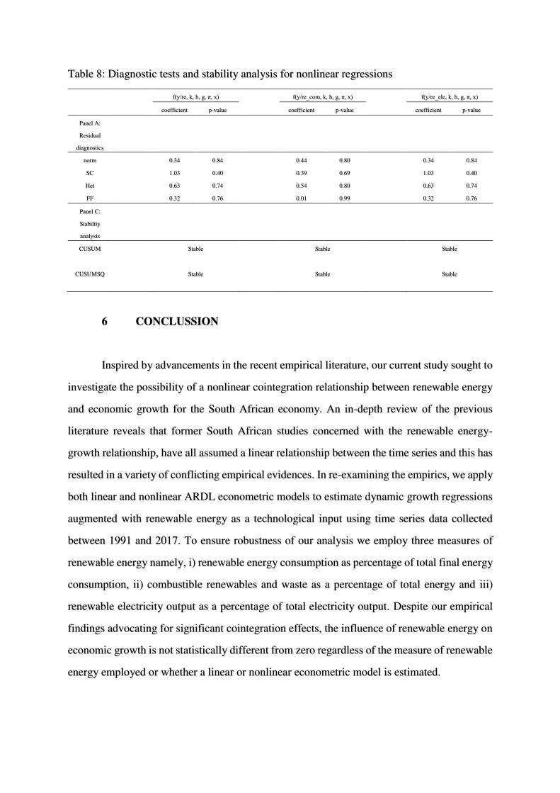
Table 8: Diagnostic tests and stability analysis for nonlinear regressions

f(y/re, k, h, g, π, x) f(y/re_com, k, h, g, π, x) f(y/re_ele, k, h, g, π, x)

coefficient p-value coefficient p-value coefficient p-value

Panel A:

Residual

diagnostics

norm 0.34 0.84 0.44 0.80 0.34 0.84

SC 1.03 0.40 0.39 0.69 1.03 0.40

Het 0.63 0.74 0.54 0.80 0.63 0.74

FF 0.32 0.76 0.01 0.99 0.32 0.76

Panel C:

Stability

analysis

CUSUM

Stable Stable Stable

CUSUMSQ

Stable Stable Stable

6 CONCLUSSION

Inspired by advancements in the recent empirical literature, our current study sought to

investigate the possibility of a nonlinear cointegration relationship between renewable energy

and economic growth for the South African economy. An in-depth review of the previous

literature reveals that former South African studies concerned with the renewable energy-

growth relationship, have all assumed a linear relationship between the time series and this has

resulted in a variety of conflicting empirical evidences. In re-examining the empirics, we apply

both linear and nonlinear ARDL econometric models to estimate dynamic growth regressions

augmented with renewable energy as a technological input using time series data collected

between 1991 and 2017. To ensure robustness of our analysis we employ three measures of

renewable energy namely, i) renewable energy consumption as percentage of total final energy

consumption, ii) combustible renewables and waste as a percentage of total energy and iii)

renewable electricity output as a percentage of total electricity output. Despite our empirical

findings advocating for significant cointegration effects, the influence of renewable energy on

economic growth is not statistically different from zero regardless of the measure of renewable

energy employed or whether a linear or nonlinear econometric model is estimated.

So, what is there to learn from our current study. Firstly, our findings resemble a bulk

majority of previous South African studies which have found no influence of renewable energy

on economic growth (Al-mulali et al. (2013), Tawari et al. (2015), Cho et al. (2015) and

Bhattacharya et al. (2016)). Considering that these former studies relied on linear frameworks

whereas our study makes use of nonlinear models, the common finding of no relationship

between renewable energy and growth pushes the literature closer to a mutual consensus.

Secondly, the insignificance of renewable energy towards economic growth indicates that

South Africa may not yet be ready to make a full transition into an economy dominated by

renewable energy sources. On the forefront of concerns facing renewable energy dependency

are the anticipated job losses expected to occur in the mining sector which could further distort

an already fragile labour market. Another concern which may serve as a hindrance to growth

opportunities for renewable energy is that the market structure for energy in South Africa is

monopolized by the government parastatal, ESKOM, and hence renewable energy cannot

feasibly compete with traditional, fossil fuel dominated of energy production in terms of both

productivity and employment creation. However, with escalating global environmental

pressures, it is in the best interest of the South African government to pursue renewable energy

strategies by particularly focusing on legislative issues prohibiting the uptake of renewable

energy sources and the limited access of independent power producers to the national energy

grid.

REFERENCES

Akarca A. and Long T. (1980), “Relationship between energy and GNP: a re-examination”,

Journal of Energy Finance and Development, 5(2), 326-331.

Al-mulali U., Fereidouni H., Lee J. and Sab C. (2013), “Examining the bi-directional long-

run relationship between renewable energy consumption and GRP growth”, Renewable and

Sustainable Energy Reviews, 22, 209-222.

Alper A. and Oguz O. (2016), “The role of renewable energy consumption in economic

growth: Evidence from asymmetric causality”, Renewable and Sustainable Energy Reviews,

60, 953-959.

Apergis N. and Payne J. (2010), “Renewable energy consumption and economic growth:

Evidence from a panel of OECD countries”, Energy Policy, 38(1), 656-660.

Apergis N. and Payne J. (2011), “On the causal dynamics between renewable and non-

renewable energy consumption and economic growth in developed and developing

countries”, Energy Systems, 2(3-4), 299-312.

Bhattacharya M., Paramati S., Ozturk I. and Bhattacharya S. (2016), “The effect of renewable

energy consumption on economic growth: Evidence from top 38 countries”, Applied Energy,

162(15), 733-741.

Cho S., Heo E. and Kim J. (2015), “Causal relationship between renewable energy

consumption and economic growth: Comparison between developed and less-developed

countries”, Geosystem Engineering, 18(6), 284-291.

Department of Energy (2003), “White Paper on Renewable Energy”, Retrieved from:

http://unfccc.int/files/meetings/seminar/application/pdf/sem_sup1_south_africa.pdf

Department of Energy (2015), “State of Renewable Energy in South Africa”, Retrieved from:

http://www.gov.za/sites/www.gov.za/files/State of Renewable Energy in South Africa_s.pdf

Department of Energy (2011), “Integrated Resource Plan for Electricity 2010-2030”,Retrived

from: http://www.energy.gov.za/IRP/irp files/IRP2010_2030_Final_Report_20110325.pdf

Department of Energy (2018), “Integrated Resource Plan 2018”,Retrieved from:

http://www.energy.gov.za/IRP/IRP-Update-018/IRP2010_2030_Final_Report_20110325.pdf

Engle R. and Granger C. (1987), “Co-integration and error correction: Representation,

estimation, and testing”, Econoemtrica, 55(2), 251-276.

Eskom (2016), “Integrated Report”, Retreived from:

www.Eskom.co.za/IR2016/Documents/Eskom_integrated_report_2016.pdf.

Fang Y. (2011), “Economic welfare impacts from renewable energy consumption: The China

experience”, Renewable and Sustainble Energy Reviews, 15(9), 5120-5128.

Greenpeace (2011), “Powering the future: Renewable energy roll-out in South Africa”,

Johannesburg.

Hwang D. and Gum B. (1991), “The causal relationship between energy and GNP: The case

of Taiwan”, The Journal of Energy and Development, 16(2), 219-226.

Inglesi-Lotz R. (2016), “The impact of renewable energy consumption to economic growth:

A panel data application”, Energy Economics, 53, 58-63.

IRENA (2015), “The Global Energy Transformation: A Roadmap to 2050”, Retrieved from

http://www.irena.org/publications/2018/Apr/Global-Energy-Transition-A-Roadmap-to-2050.

Johansen S. (1991), “Estimation and hypothesis testing of cointegration vectors in Gaussian

vector autoregressive models”, Econometrica, 59(6), 1551-1580.

Kahia M., Aissa M. and Lanouar C. (2017), “Renewable and non-renewable energy use –

economic growth nexus: The case of MENA net oil importing countries”, Renewable and

Sustainable Energy Reviews, 71, 127-140.

Khobai H. and Le Roux P. (2018), “Does renewable energy consumption drive economic

growth: Evidence from granger-causality technique”, International Journal of Energy

Economics and Policy, 8(2), 205-212.

Kocak E. and Sarkgunesi A. (2017), “The renewable energy and economic growth nexus in

Balkan Sea and Balkan countries”, Energy Policy, 100(C), 51-57.

Kraft J. and Kraft A. (1978), “On the relationship between energy and GNP”, Journal of Energy

Development, 3, 401-403.

Lin B. and Moubarak M. (2014), “Renewable energy – economic growth nexus for China”,

Renewable and Sustainable Energy Reviews, 40, 111-117.

Malangeni L. and Phiri A. (2018), “Education and economic growth in Post-Apartheid South

Africa: An autoregressive distributive lag approach”, International Journal of Economics and

Financial Issues, 8(2), 101-107.

Mbarek M., Abdelkafi I. and Feki R. (2018), “Nonlinear causality between renewable energy,

economic growth, and unemployment: Evidence from Tunisia”, Journal of Knowledge

Economy, 9(2), 694-702.

Menegaki A. (2011), “Growth and renewable energy in Europe: A random effect model with

evidence for neutralitiy hypothesis”, Energy Economics, 33(2), 257-263.

Ocal O. and Aslan A. (2013), “Renewable energy consumption-economic growth nexus in

Turkey”, Renewable and Sustainable Energy Reviews, 28, 494-499.

Pesaran M., Shin Y. and Smith R. (2001), “Bounds testing approaches to the analysis of level

relationships”, Journal of Econometrics, 16(3), 289-326.

Phiri A. and Nyoni B. (2016), “Re-visiting the electricity-growth nexus in South Africa”,

Studies in Business and Economics, 11(1), 97-111.

Phiri A. (2018), “Nonlinear impact of inflation on economic growth in South Africa: A

smooth transition regression analysis”, International Journal of Sustainable Economy, 10(1),

1-17.

Rafindadi A. and Ozturk I. (2017), “Impacts of renewable energy consumption on the

German economic growth: Evidence form combined cointegration test”, Renewable and

Sustainable Energy Reviews, 75, 1130-1141.

Sardorsky P. (2009), “Renewable energy consumption and income in emerging economies”,

Energy Economics, 37(10), 4021-4028.

Sebri M. and Ben-Salha O. (2014), “On the causal dynamics between economic growth,

renewable energy consumption, CO2 emissions and trade openness: Fresh evidence from

BRICS countries”, Renewable and sustainable Energy Reviews, 39, 14-23.

Shahbaz M., Loganathan N., Zeshan M. and Zaman K. (2015), “Does renewable energy

consumption add in economic growth? An application of the auto-regressive distributive lag

model in Pakistan”, Renewable and Sustainable Energy Reviews, 44, 576-585.

Shin Y., Yu B. and Greenwood-Nimmo M. (2014), “Modelling asymmetric cointegration and

dynamic multipliers in a nonlinear ARDL framework”, Festsschrift in honor of Peter

Schmidt: Econometric Methods and Applications, eds. By R. Sickels and W. Horace,

Springer, 281-314.

Sorensen B. (1991), “A history of renewable energy technology”, Energy Policy, 19(1), 8-12.

Sunde T. (2017), Foreign direct investment, exports and economic growth: ARDL and

causality analysis for South Africa”, Research in International Business and Finance, 41,

434-444.

Tawari A., Apergis N. and Olayeni O. (2015), “Renewable and non-renewable energy

production and economic growth in sub-Saharan Africa: A hidden cointegration approach”,

Applied Economics, 47(9), 861-882.

Tugcu C., Ozturk I., Aslain A. (2012), “Renewable and non-renewable energy consumption

and economic growth revisited: Evidence from G7 countries”, Energy Economics, 34, 1942-

1950.

Walwyn D. and Brent A. (2015), “Renewable energy gathers steam in South Africa”,

Renewable and Sustainable Energy Reviews, 41(C), 390-401.

Yu E. and Choi J. (1985), “The causal relationship between energy and GNP: An

international comparison”, The Journal of Energy and Development, 10(2), 249-272.

Yu E. and Hwang B. (1984), “The relationship between energy and GNP: Further results”,

Energy Economics, 6(3), 186-190.

Yu E. and Jin J. (1992), “Cointegration tests of energy consumption, income and

employment”, Resources and Energy, 14(3), 259-266.