Relating Hyperspectral Image Bands and …...Remote sensing has been used to investigate a –183–...

1. Introduction

Precision agriculture requires efficient and accurate

quantification of sub-field variations in crop yields

and those factors which may influence yields.

Remote sensing has been used to investigate a

–183–

Relating Hyperspectral Image Bands and Vegetation Indices to Corn and Soybean Yield

Gab-Sue Jang*†, Kenneth A. Sudduth**, Suk Young Hong***, Newell R. Kitchen**, and Harlan L. Palm****

Chungnam Development Institute, Daejeon, Republic of Korea*

USDA-ARS Cropping Systems and Water Quality Research Unit, Columbia, Missouri, USA**

National Institute of Agricultural Science and Technology, Suwon, Republic of Korea***

Department of Agronomy, University of Missouri, Columbia, Missouri, USA****

Abstract : Combinations of visible and near-infrared (NIR) bands in an image are widely used forestimating vegetation vigor and productivity. Using this approach to understand within-field grain cropvariability could allow pre-harvest estimates of yield, and might enable mapping of yield variations withoutuse of a combine yield monitor. The objective of this study was to estimate within-field variations in cropyield using vegetation indices derived from hyperspectral images. Hyperspectral images were acquired usingan aerial sensor on multiple dates during the 2003 and 2004 cropping seasons for corn and soybean fieldsin central Missouri. Vegetation indices, including intensity normalized red (NR), intensity normalized green(NG), normalized difference vegetation index (NDVI), green NDVI (gNDVI), and soil-adjusted vegetationindex (SAVI), were derived from the images using wavelengths from 440 nm to 850 nm, with bandsselected using an iterative procedure. Accuracy of yield estimation models based on these vegetation indiceswas assessed by comparison with combine yield monitor data. In 2003, late-season NG provided the bestestimation of both corn (r2 = 0.632) and soybean (r2 = 0.467) yields. Stepwise multiple linear regressionusing multiple hyperspectral bands was also used to estimate yield, and explained similar amounts of yieldvariation. Corn yield variability was better modeled than was soybean yield variability. Remote sensing wasbetter able to estimate yields in the 2003 season when crop growth was limited by water availability,especially on drought-prone portions of the fields. In 2004, when timely rains during the growing seasonprovided adequate moisture across entire fields and yield variability was less, remote sensing estimates ofyield were much poorer (r2 < 0.3).

Key Words : Hyperspectral Remote Sensing, Vegetation Indices, Crop Yield.

Korean Journal of Remote Sensing, Vol.22, No.3, 2006, pp.183~197

Received 4 May 2006; Accepted 21 June 2006.†Corresponding Author: G. S. Jang ([email protected])

02장갑수(183-197) 2006.8.11 9:48 AM 페이지183

number of agricultural attributes, including crops,

soils, water, and climate, traditionally at regional or

larger scales. More recently, increased spatial

resolution has allowed remote sensing to be applied

to investigate many of these same attributes at the

sub-field scales important in precision agriculture.

To date, multispectral imaging has been one of the

most common remote sensing approaches used to

investigate field attributes. These multispectral

images, acquired from aircraft or satellite, quantify

the reflectance characteristics of a target in a few

relatively wide wavelength bands, often representing

blue, green, red, and near infrared (NIR) wavelengths

(Lillesand et al., 2004).

A recent development in agricultural remote

sensing has been the use of aerial hyperspectral

imaging systems, where reflectance is quantified in a

large number of relatively narrow wavelength bands.

Improvements in computer and imaging technology

have made such systems more affordable, and the

ability to schedule aerial image acquisitions has

allowed researchers to collect ground data

simultaneously with the images. In an effort to exploit

the improved spatial and spectral resolution of

airborne hyperspectral imaging systems, a number of

researchers have investigated their use in precision

agriculture (e.g., Deguise et al., 1998; Willis et al.,

1998; Mao, 1999; Yang and Everitt, 2002).

Several studies have investigated the use of aerial

images to estimate within-field yield variability. Yang

et al. (2004) applied stepwise regression analysis to

128-band aerial hyperspectral images obtained on a

single date from two grain sorghum fields. They were

able to account for 69% of the yield variability with

the best four-band combination, and 82% of the yield

variability with best seven-band combination. The

best single bands for yield estimation in the two fields

were 510 and 782 nm. Thenkabail et al. (2000)

related hyperspectral vegetation indices to crop

characteristics, including biomass, leaf area index,

plant height, and yield, explaining 64% to 88% of the

variability with the best models. They identified four

important wavelength ranges, 650-700 nm, 500-550

nm, 900-940 nm, and the water-sensitive NIR region

centered at 982 nm. Aerial multispectral images were

used to model yield variation by GopalaPillai and

Tian (1999). Normalized intensity, averaged over

NIR, red, and green bands, gave the best estimation

of corn yield, with an r2 of 0.87. Yang and Everitt

(2002) also used multispectral images to estimate

yield for grain sorghum. Images taken around the

time of peak vegetative development explained 63,

82, and 85% of yield variability for three grain

sorghum fields. The single best spectral variable for

estimating yield was the intensity normalized green

(NG, the ratio of green to NIR reflectance) index.

In our previous work, Hong et al. (2001) applied

correlation and regression analysis to 120-band aerial

hyperspectral data to estimate within-field variations

in corn and soybean yield over two fields and two

years. Using a vegetative index (VI) approach, we

accounted for up to 52% of corn yield variability, but

only 18% of soybean yield variability, with an

intensity normalized green (NG, the ratio of green to

NIR reflectance) index providing the best results.

Better results were obtained with principal

components regression, accounting for up to 70% of

corn yield variability and 39% of soybean yield

variability. With these results based on only two

fields and two years, additional data collection and

analysis was needed.

The goal of this study was to investigate the

relationship of hyperspectral image data to within-

field corn and soybean yield variation under rainfed

production in central Missouri. Specific objectives

were to (1) extract hyperspectral image-derived

vegetation indices and relate them to within-field

variations in crop yield, (2) determine the best

Korean Journal of Remote Sensing, Vol.22, No.3, 2006

–184–

02장갑수(183-197) 2006.8.11 9:48 AM 페이지184


–185–

wavelengths to estimate yield, and (3) develop

estimated yield maps for comparison with combine

yield monitor data.

2. Materials and Methods

1) Study Sites

The two fields (Field 1, 35 ha, and Field 2, 13 ha)

used in this study were located within 3 km of each

other near Centralia, in central Missouri. Soils found

at these fields are somewhat poorly drained claypan

soils of the Mexico series and the Adco series.

Surface textures range from silt loam to silty clay

loam. The subsoil claypan horizon(s) are silty clay

loam, silty clay or clay, and commonly contain as

much as 50 to 60% smectitic clay. Within each study

field, topsoil depth above the claypan (depth to the

first B horizon) ranged from less than 10 cm to

greater than 100 cm.

Data documenting within-field variations in crop

yields, soil properties, and other factors have been

obtained since 1993 for Field 1 and since 1996 for

Field 2. Although precision agriculture technologies

have been employed for data collection, no variable

application of crop inputs occurred during the time of

this study. Additional information can be found in

Lerch et al. (2005).

2) Image and Yield Data Collection

Aerial hyperspectral images were obtained using the

AISA1) sensor (Airborne Imaging Spectrometer for

Applications, Specim Ltd., Finland) mounted in a

single-engine light aircraft and operated by the Center

for Advanced Land Management Information

Technologies (CALMIT) at the University of

Nebraska, Lincoln, Nebraska. A key feature of the

AISA system is a downwelling irradiance sensor

mounted on top of the aircraft, allowing calculation of

apparent reflectance at the sensor. Research has verified

that the at-sensor reflectance can be used as a surrogate

for target reflectance, eliminating the need to deploy

calibration standards on the ground, yet facilitating

multi-temporal analysis (Charles Walthall, USDA-

ARS, Beltsville, MD, personal communication).

AISA images of at-sensor apparent reflectance

were collected three times per year during the 2003

and 2004 cropping seasons. The AISA data were

collected in 20 bands during 2003, and in 24 bands

during 2004 with center wavelengths ranging from

440 to 850 nm (Table 1). The spatial resolution was

1.5 m in 2003 and 2 m in 2004. The image vendor,

CALMIT, provided the ability to select from several

configuration options. In each year, we selected the

smallest pixel size that would provide a swath width

sufficient for imaging of the research sites without the

need to mosaic overlapping flightlines. Because of

data throughput considerations, the maximum

number of bands available from the AISA sensor was

related to the pixel size selected. The number of

bands obtained each year was the maximum for that

pixel size, and the center wavelengths were pre-

determined by the CALMIT configuration option.

Table 2 describes the crops, dates of field operations,

and descriptive yield statistics for each year of image

collection.

Grain yield measurements were obtained using a

Gleaner R-42 combine (AGCO Corporation, Duluth,

Georgia, USA) equipped with a Yield Monitor 2000

yield sensing system (Ag Leader Technology, Ames,

Iowa, USA) and differential global positioning

system (GPS) receiver with approximately 1-m

accuracy. Yield data were recorded on a 1-s interval

1) Mention of trade names or commercial products inthis article is solely for the purpose of providingspecific information and does not implyrecommendation or endorsement by the U.S.Department of Agriculture or cooperating institutions.

02장갑수(183-197) 2006.8.11 9:48 AM 페이지185

while the combine harvested the field at

approximately 3 m/s. Harvest width for corn was 3

m, while the harvest width for soybean was 4.5 m.

Individual points where yield data were unreliable

were removed so that the resulting yield map

represented the actual yield as closely as possible.

Based on our experience (Drummond and Sudduth,

2005) and that of others (e.g., Robinson and

Metternicht, 2005), yield data points were removed

for reasons such as GPS positional error, abrupt

combine speed changes, significant ramping of grain

flow during entering or leaving the crop, unknown or

variable crop swath width, and other outlying values.

Our intent was to err on the side of caution, removing

any questionable data from the point dataset so that

the interpolation procedure would not be significantly

affected by a few outliers.

Cleaned yield monitor data was interpolated with

the geostatistical technique of kriging. The best-fitting

semivariogram interpolation function was determined

separately for each year and applied to estimate yield

for each 5-m square grid within the field. Kriging was

chosen over other interpolation procedures, such as

inverse distance weighting, because of its ability to

quantify uncertainty in the yield estimates,

information useful in the data filtering process. We

(Birrell et al., 1996) and others (Robinson and

Metternicht, 2005) have shown that yield estimates

from kriging with various interpolation parameters

and from inverse distance weighting are quite similar,

due to the high spatial density of the original yield

monitor data.


–186–

Table 1. Band centers and bandwidths (as FWHM, full width at half maximum) of the AISA system, as configured for this study.

Band no. 2003 2004 Band no. 2003 2004Band center FWHM Band center FWHM Band center FWHM Band center FWHM

(nm) (nm) (nm) (nm) (nm) (nm) (nm) (nm)

1 440.5 6.3 440.5 6.3 13 700.1 3.4 684.8 5.2

2 473.7 6.3 473.7 6.3 14 705.3 3.4 691.6 5.2

3 499.8 4.7 499.8 4.7 15 710.4 3.4 700.1 5.2

4 542.4 4.7 542.4 4.7 16 715.5 3.4 705.3 5.2

5 550.3 4.7 550.3 4.7 17 727.5 3.4 710.4 5.2

6 561.4 4.7 561.4 4.7 18 763.4 3.4 715.5 5.2

7 585.1 4.7 585.1 4.7 19 819.8 3.4 727.5 5.2

8 609.2 5.2 609.2 5.2 20 848.9 3.4 763.4 5.2

9 651.0 5.2 621.4 5.2 21 773.7 5.2

10 670.1 5.2 631.8 5.2 22 807.9 5.2

11 684.8 5.2 651.0 5.2 23 819.8 5.2

12 691.6 5.2 670.1 5.2 24 848.9 5.2

2003 2004 2003 2004

Band no. Band center FWHM Band center FWHM Band no. Band center FWHM Band center FWHM (nm) (nm) (nm) (nm) (nm) (nm) (nm) (nm)

Table 2. Crop, field activity dates, and yield information for the two fields used in this study.

Year Field Crop Field activity date Mean yield Min. yield Max. yield Yield SDSeeding Harvesting Imaging---------------- (Mg/ha) --------------

2003 1 Corn 5/22-5/27 10/16, 10/24 6/27, 7/16, 8/22 2.0 0.0 8.6 2.9

2003 2 Soybean 6/9 10/23 6/27, 7/16, 8/22 1.6 0.4 3.3 0.5

2004 1 Soybean 5/21, 5/22 10/4-10/7, 12/14 7/7, 8/5, 8/30 3.3 0.2 4.3 0.3

2004 2 Soybean 6/4 12/14 7/7, 8/5, 8/30 3.1 0.1 4.4 0.6

Year Field CropField activity date Mean yield Min. yield Max. yield Yield SD

Seeding Harvesting Imaging ---------------- (Mg/ha) --------------

02장갑수(183-197) 2006.8.11 9:48 AM 페이지186

3) Image and Yield Data Processing

Geometric distortion observed in the AISA images

was adjusted by a rubber sheeting model. Data used

for geo-referencing included accurate surveyed field

boundary vector data and a 1-m resolution QuickBird

image taken on June 7, 2002. ArcGIS 9 (ESRI,

Redlands, CA) and ERDAS IMAGINE 8.7 (Leica

Geosystems, Norcross, GA) were jointly used to

manage and analyze the AISA images and the yield

data for two fields.

The vegetation indices used to relate to yield data

were intensity normalized red (NR = NIR/Red; Birth

and McVey, 1968), intensity normalized green (NG =

NIR/Green; Yang and Everitt, 2002), normalized

difference vegetation index (NDVI = (NIR - red) /

(NIR + red); Rouse et al., 1974), green NDVI

(gNDVI = (NIR - green) / (NIR + green); Yang and

Everitt, 2002), and soil-adjusted vegetation index

(SAVI = (1 + L) (NIR - red) / (NIR + red + L);

Huete, 1988). Because Jensen (2000) found that an L

value of 0.5 in SAVI minimized soil brightness

variations, we also used L = 0.5.

Geo-rectified AISA images were combined with

the yield data, creating a common dataset for relating

AISA-derived vegetation indices to soybean and corn

yields. The combined dataset was imported into

ArcGIS, and the resolution of the image data was

reduced to 5 m, coincident with the 5-m combine

yield data grid. The resulting datasets contained

approximately 11,700 points for Field 1 and 3,800

points for Field 2. Correlation and regression

procedures were used to relate vegetation indices to

measured yield and to obtain equations for estimating

yield as a function of vegetation indices. Correlation

analysis was also performed to relate individual band

reflectance to yield, and stepwise regression was

applied to determine the optimum band combinations

for estimating yield.

3. Results and Discussion

1) Reflectance Trends over the GrowingSeason

Figure 1 shows gray-scale AISA images for the 12

datasets used in this study. These images show details

of the crop growth variation within the fields. In these

images, areas with more vegetation are darker, while

areas with less vegetation are lighter.

Spectral signatures for the 20 bands obtained in

2003 and the 24 bands obtained in 2004 were

calculated (Figure 2). On June 24, 2003, the corn in

Field 1 and the soybean in Field 2 were at 28 days

after seeding (DAS) and 16 DAS, both in early

vegetative stages. The corn and soybean had low (less

than 20%) reflectance due to small leaf area and

influence of soil background. Yang et al. (2004)

reported that the soil background effect was

approximated by a straight line with a small positive

slope, similar to the behavior seen for this image date

(Figure 2). On July 16, 2003, the corn in Field 1 was

at a late vegetative stage (50 DAS), and the soybean

in Field 2 was in a mid-vegetative stage V4 (38

DAS). The reflectance of the corn in Field 1 had

increased considerably in the NIR (715 to 849 nm)

wavelengths, while the reflectance of the soybean in

Field 2 had not changed much, due to the smaller

amount of canopy growth for the soybean during the

intervening 22 days. On August 22, 2003, the corn in

Field 1 and the soybean in Field 2 were both in the

reproductive stage. By this date, corn reflectance had

plateaued in the NIR region, while soybean

reflectance was continuing to increase (Figure 2).

On July 7, 2004, soybean in Field 1 was at 45 DAS

and the soybean in Field 2 was at 31 DAS. In both

fields, the NIR reflectance was higher than the NIR

reflectance of the 2003 soybean crop at a similar point

in the season (Field 2 soybean on July 16, 2003 at 38


–187–

02장갑수(183-197) 2006.8.11 9:48 AM 페이지187

DAS), presumably due to the better growing

conditions in 2004. The reflectance of soybean in both

fields increased continuously over time in 2004. The

one exception was that the Field 1 soybean crop had a

lower mean reflectance on August 30, 2004 than it did

on August 5, 2004. An outbreak of powdery mildew

in Field 1 shortly before the August 30 imaging may

have lowered the NIR reflectance of the crop.


–188–

Figure 1. AISA images for study sites at three measurement dates during each of the 2003 and2004 growing seasons.

Figure 2. Mean reflectance in AISA image bands for the two fields in 2003 and 2004. Bars represent within-field standard deviationat each wavelength.

02장갑수(183-197) 2006.8.11 9:48 AM 페이지188

Lorenzen and Jensen (1989) found changes in the

spectral properties of barley leaves due to powdery

mildew and theorized that canopy-scale differences

might also be seen, primarily due to differences in

canopy structure between healthy and diseased crops.

In general, reflectance in the visible region (440 to

700 nm) was below 0.1. The reflectance in the shorter

wavelength portion of the NIR region (700 nm to 780

nm) increased rapidly with wavelength. The

reflectance in the longer wavelength portion of the

NIR region (780 nm to 850 nm) was higher, and did

not increase as quickly as a function of wavelength.

As the cropping season progressed, reflectance

changed little or decreased slightly in the visible

wavelengths, but reflectance increased in the NIR

except for Field 1 in 2003 (corn) and 2004 (soybean).

The corn on August 22, 2003 had lower reflectance

because the crop had begun to senesce somewhat

prematurely due to the dry growing conditions. As

noted above, the Field 1 soybean on August 30, 2004

was presumed to have lower reflectance because of

the existence of powdery mildew.

2) Correlation of Reflectance to Yield

Scatter plots of grain yield as a function of single-

band reflectance in selected green, red, and NIR

bands were examined for trends (data not shown).

There was no readily apparent relationship between

single-band reflectance and either corn or soybean

yield early in the growing seasons. However, linear

relationships did appear at later imaging dates,

particularly in 2003. Correllograms plotted as a

function of wavelength for all fields, years, and

imaging dates (Figure 3) supported this observation.

Overall, reflectance had a negative correlation with

yield in visible bands but positive correlation with

yield in the NIR region. The one exception to this

was soybean in Field 2 in 2004, which exhibited


–189–

Figure 3. Correlation coefficients (r) between reflectance in individual AISA bands and grain yield.

02장갑수(183-197) 2006.8.11 9:48 AM 페이지189

some positive correlations between yield and visible

reflectance (Figure 3). There were also differences in

the correlation of reflectance with yield between 2003

and 2004. As the growing season progressed,

correlations increased for 2003 corn and soybean,

while soybean in 2004 had lower correlation to yield

(Field 1) or an irregular trend of correlation with yield

(Field 2) through the season.

We attribute differences in correlation trends and

levels between these two years primarily to

differences in precipitation between the growing

seasons. Total rainfall during the cropping season

(May to September) in 2003 (624 mm) was higher

than in 2004 (531 nm). However, during the high

plant-water-use months of July and August, rainfall in

2004 (363 mm) was more than twice the amount

received in 2003 (150 mm). The claypan soils found

on these fields have low water holding capacity,

especially on eroded sideslope areas. Because of this,

timely mid-summer rainfall is critical for good crop

growth and yield. In years like 2003, when rainfall is

lacking during the mid to late part of the growing

season, crop growth and grain yields will generally be

much higher in less eroded areas of the field where

plant available water is greater (Kitchen et al., 2005).

In years with sufficient rainfall, like 2004, yields will

generally be higher and less variable. What variability

does occur will more likely be due to factors other

than stress due to lack of available water. Because

yields may be less correlated to biomass in these

years, it follows that they will also be less correlated

to VI measurements.

3) Correlation of Vegetation Indices to Yield

VIs were calculated with all possible combinations

of AISA bands, and correlation maps (Figure 4) were

used to visually examine trends in correlation of the

VIs to yields. Generally, correlations of VI to yield

increased during the growing season. Figure 4 presents

the time sequence of correlation maps for Field 1 corn

in 2003, showing this increase in correlation coefficient

as the crop matured. Figure 4 also shows that yield was

best correlated to ratios that combined longer-

wavelength NIR reflectance with blue, green, red, or

shorter-wavelength NIR reflectance.

When comparing correlation maps developed with

the various VIs, there was little difference in the

correlation coefficients with yield. In general, NDVI

had a slightly lower correlation to yield than other

VIs. In some fields and years, RVI provided the

highest correlation, while SAVI was better for other

datasets (Table 3). The best band combinations also

varied among datasets (Table 3). For the corn field on

August 22, 2003 (87 DAS), the best combination for

all three VIs was the longer wavelength portion of the

NIR band (849 nm) and the shorter wavelength

portion of the NIR (716 nm). The best band

combination for soybean on August 22, 2003 (75

DAS) was the longer wavelength portion of NIR (849

nm) and the blue band (441 or 474 nm) in RVI and

SAVI, while NDVI used two short-NIR bands. On

August 30, 2004, with better growing conditions in

Field 1, the best RVI, NDVI, and SAVI indices

combined 700 nm (red) and 474 nm (blue) bands. For

the three field-years described above, the highest

correlations between VIs and yield were all seen for

the last imaging date of the season. However,

soybean VIs in Field 2 had a better correlation to

yield on August 5, 2004 (60 DAS) than on August

30, 2004 (86 DAS) (data not shown). It may be that

the good growing conditions in 2004 caused the

soybean canopy to grow enough by the last imaging

date that the VIs were saturated and unable to

discriminate differing yield levels, making

correlations better with the image taken earlier.

The preceding results were derived using all bands

in the AISA image, rather than from the standard


–190–

02장갑수(183-197) 2006.8.11 9:48 AM 페이지190

NIR-red or NIR-green VI combinations. Additionally,

we examined VIs calculated using the standard

combinations of green (500 to 600 nm), red (600 to

700 nm), and NIR (700 to 850) wavelengths and

graphed the results for the best image of each field in

2003 (Figure 5).

For the one corn dataset (Field 1, 2003), VIs

calculated from the August 22 image had

considerably different correlations with yield

depending on which NIR band was used.

Correlations were highest (r > 0.8) using the longer-

wavelength portion of the NIR region (bands 18 to

20, 763 to 849 nm), and also less sensitive to the

choice of the visible band used in the calculation


–191–

Figure 4. Correlation coefficients obtained between corn yield for Field 1 in 2003 and ratio vegetativeindex (RVI), using all possible combinations of the 20 available AISA wavelengths. Reflectancein the y-axis band is in the denominator, and reflectance in the x-axis band is in the numeratorof the RVI.

Table 3. The best combination of wavelengths for each VI andthe resulting correlation of that best VI to yield.

Date Field VI Visible NIR r(crop) wavelength wavelength

(nm) (nm)

August 22, 1RVI 716 849 0.855

2003 (corn)NDVI 716 849 0.833SAVI 716 849 0.823

August 22, 2RVI 474 849 0.689

2003 (soybean)NDVI 728 763 0.660SAVI 441 849 0.712

August 30, 1RVI 700 474 0.332

2004 (soybean)NDVI 474 700 -0.331SAVI 474 700 -0.360

August 5, 2RVI 728 820 0.440

2004 (soybean)NDVI 728 820 0.441SAVI 763 774 0.407

Field Visible NIR

Date(crop)

VI wavelength wavelength r(nm) (nm)

02장갑수(183-197) 2006.8.11 9:48 AM 페이지191

(Figure 5). Correlation coefficients of VIs with yield

were lower and more sensitive to the choice of the

visible band when using the shorter-wavelength

portion of the NIR region (bands 14 to 17, 705 to 728

nm). Similar, but less pronounced, trends were seen

for the 2003 soybean crop on Field 2 (Figure 5).

When restricting the wavelengths in the VI

calculations to green, red, and NIR, the NR index

using 763 nm and 700 nm showed the highest

correlation (r = 0.829) to 2003 corn yield and the NG

index using 849 nm and 550 nm showed the highest

correlation (r = 0.678) to 2003 soybean yield. In


–192–

Figure 5. Correlation coefficients of NG, NR, NG, gNDVI, rNDVI (or NDVI), and SAVI from AISA images obtained on August22, 2003 in Fields 1 and 2.

02장갑수(183-197) 2006.8.11 9:48 AM 페이지192

2004, the August 5 image gave higher correlations

(max r = 0.380) than the August 30 image (max r =

0.265). The gNDVI index using 849 nm and 542 nm

showed the highest correlation (r = 0.380) with 2004

soybean yield in Field 2 (data not shown). No VI

calculation provided a correlation greater than 0.3

with 2004 soybean yield in Field 1.

4) Estimating Yield and Generating YieldMaps

Regressions estimating yield from VI were

completed for band pairs with the best correlations in

Figure 5. Longer-wavelength NIR bands, 820 nm and

849 nm, were combined with each visible band and

the regression results compared. In 2003, the best corn

yield estimates were obtained with an NG index, using

the 561 nm and 849 nm bands (r2 = 0.632), while the

best soybean yield estimates were also obtained with

an NG index, using the 550 nm and 849 nm bands (r2

= 0.467). These results are similar to those reported by

Yang and Everitt (2002), who found that using a

combination of a longer-wavelength (845-857 nm)

NIR band and a mid-green (555-565 nm) band in an

NG equation provided better estimates of sorghum

yield than did other VIs. In contrast to the 2003

results, VI regressions using 2004 data explained less

than 20% of within-field yield variability.

In addition to VI regressions, we developed

models to estimate yield from combinations of AISA

band reflectances using stepwise multiple linear

regression. Before the analysis, bands were examined

for multicollinearity using the variance inflation

factor (VIF), which indicates how much the variances

of the estimated regression coefficients are inflated as

compared to when the predictor variables are not

linearly related (Neter et al., 1986; SAS Institute,

1999). Bands with a high VIF were removed from the

subsequent stepwise regression analysis. The best

stepwise models were selected as the ones with the

highest R2 and with all bands in the model

statistically significant at the 0.0001 level. Using

these criteria, the best models obtained for each

image date contained from one to six reflectance

terms (Table 4). The wavelength most frequently

used in the regression models was 440 nm (9 times

out of 12). Bands at 473, 715, and 763 nm were also

used frequently in the regression models.

Table 4 shows the wavelengths used in the best


–193–

Table 4. Wavelengths used in multiple linear models relating yield to reflectance in AISA images for Field 1 and Field 2 in 2003 and2004. All terms remaining in the models were significant at the 0.0001 level.

Field Date 440 473 499 542 585 684 700 705 710 715 727 763 820 848 R2 Std. Err. (Mg/ha)

1 06/24/03 ● ● ● ● ● 0.152 0.90

1 07/16/03 ● ● ● ● 0.359 0.78

1 08/22/03 ● ● ● ● ● 0.701 0.54

2 06/24/03 ● ● ● ● 0.246 0.42

2 07/16/03 ● ● ● 0.150 0.45

2 08/22/03 ● ● ● 0.456 0.36

1 07/07/04 ● ● ● ● ● 0.043 0.32

1 08/05/04 ● ● ● ● ● 0.118 0.30

1 08/30/04 ● ● ● ● ● ● 0.152 0.30

2 07/07/04 ● ● ● ● ● 0.286 0.47

2 08/05/04 ● ● ● ● 0.189 0.50

2 08/30/04 ● ● ● ● 0.200 0.50

Field Date 440 473 499 542 585 684 700 705 710 715 727 763 820 848 R2 Std. Err. (Mg/ha)

02장갑수(183-197) 2006.8.11 9:48 AM 페이지193

multiple linear model for each field and image date,

along with R2 values and standard errors. As with the

VI analysis, images obtained later in the growing

season generally gave better estimates of yield. The

August 22 image explained 70% of corn yield

variability (Field 1) and 46% of soybean yield

variability (Field 2) in 2003. As with the other

analyses, relationships between image data and yield

were poor in 2004, where no image explained over

30% of within-field yield variability (Table 4).

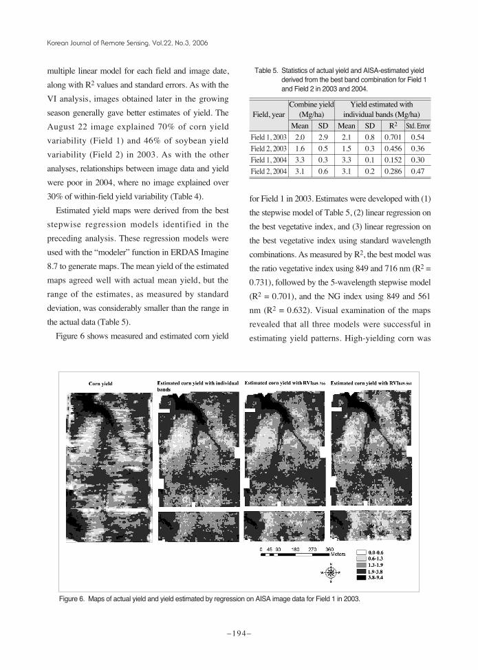
Estimated yield maps were derived from the best

stepwise regression models identified in the

preceding analysis. These regression models were

used with the “modeler” function in ERDAS Imagine

8.7 to generate maps. The mean yield of the estimated

maps agreed well with actual mean yield, but the

range of the estimates, as measured by standard

deviation, was considerably smaller than the range in

the actual data (Table 5).

Figure 6 shows measured and estimated corn yield

for Field 1 in 2003. Estimates were developed with (1)

the stepwise model of Table 5, (2) linear regression on

the best vegetative index, and (3) linear regression on

the best vegetative index using standard wavelength

combinations. As measured by R2, the best model was

the ratio vegetative index using 849 and 716 nm (R2 =

0.731), followed by the 5-wavelength stepwise model

(R2 = 0.701), and the NG index using 849 and 561

nm (R2 = 0.632). Visual examination of the maps

revealed that all three models were successful in

estimating yield patterns. High-yielding corn was


–194–

Table 5. Statistics of actual yield and AISA-estimated yieldderived from the best band combination for Field 1and Field 2 in 2003 and 2004.

Field, yearCombine yield (Mg/ha)Yield estimated withindividual bands (Mg/ha)

Mean SD Mean SD R2 Std. Error

Field 1, 2003 2.0 2.9 2.1 0.8 0.701 0.54

Field 2, 2003 1.6 0.5 1.5 0.3 0.456 0.36

Field 1, 2004 3.3 0.3 3.3 0.1 0.152 0.30

Field 2, 2004 3.1 0.6 3.1 0.2 0.286 0.47

Combine yield Yield estimated with Field, year (Mg/ha) individual bands (Mg/ha)

Mean SD Mean SD R2 Std. Error

Figure 6. Maps of actual yield and yield estimated by regression on AISA image data for Field 1 in 2003.

02장갑수(183-197) 2006.8.11 9:48 AM 페이지194

found in the lower elevations close to the drainage

way running north to south near the center of the

field. In the water-limited 2003 growing season,

crops in this area received more water, both due to

accumulation of runoff from higher portions of the

field and due to the deeper topsoil with higher water-

holding capacity. Lower yields were seen in the

eroded sideslope areas of the field, primarily due to

low water-holding capacity of the soils in those parts

of the field, coupled with loss of precipitation as

runoff (Figure 6). The main discrepancies between

measured and estimated yields were found along the

east and west edges of the field, where measured

yields were low but the aerial image indicated

relatively high biomass (Figure 1). It is possible that

yield reductions in those areas were caused by some

phenomenon that did not reduce crop biomass (e.g.,

barren plants, shading due to treeline) or by part of

the biomass seen in the images having actually been

late-season weed growth rather than crop.

Estimating corn and soybean yield using aerial

hyperspectral data appears to have some promise.

Particularly under drier growing conditions, where

within-field yield variability was large, estimated

yield maps agreed well with data obtained from

combine yield mapping. However, results in the high-

rainfall year of 2004 were not as good, presumably

due to the good growing conditions and relatively less

within-field variation. In another 2004 study, we

collected leaf area index (LAI) data at 40 points in

Field 1 within 48 hours of each hyperspectral image

acquisition using a LAI-2000 instrument (LI-COR

Biosciences, Lincoln, NE, USA). Although the range

of soybean yield across these points was similar to the

range in the entire field, there was no significant

relationship between yield and LAI (r2 < 0.07). This

unpublished finding supports our assertion that the

relatively small yield variations in 2004 were not

related to plant biomass, but likely to some other

factors that were not detectable with our analysis.

The fact that corn yield variability was better

modeled than was soybean yield variability agreed

with other results we obtained on these same fields,

during different cropping seasons and with a different

aerial hyperspectral sensor (Hong et al., 2001). In

general, the NR and NG indices were slightly more

related to yield than were NDVI, gNDVI, or SAVI,

although this trend was not completely consistent

across crops and field-years. Other researchers, and

our previous work (Hong et al., 2001), have also

found ratio indices, especially NG, to be best for

estimating within-field yield variation.

The many bands available in a hyperspectral

dataset allow much flexibility in selecting yield

estimation models. In our work, a simple stepwise

multiple linear regression incorporating band

reflectance data was slightly more predictive of yield

than VIs constructed using standard wavelength

ranges. We also obtained slightly better estimates

with some VIs constructed with non-standard

wavelengths (e.g., a ratio of two NIR bands). Further

research, incorporating data collected under different

growing conditions, would be needed to verify that

these other approaches could consistently provide

improved yield estimates. Additionally, other

modeling approaches (e.g., principal component

regression, nonlinear regression) that could make

better use of the large number of bands available in

hyperspectral images should be investigated.

4. Summary and Conclusions

Corn and soybean yield is related to many factors.

In non-irrigated systems, rainfall during the growing

season is one of the most important factors affecting

yield. In this study relating aerial hyperspectral

images to crop yield, it appeared that rainfall during


–195–

02장갑수(183-197) 2006.8.11 9:48 AM 페이지195

the growing season, and the resulting expression of

yield variability, also affected our ability to estimate

yield from image data. In 2003, when growing-

season rainfall was scarce and crops were water-

stressed, correlations between image data and yield

were relatively high. However, in 2004, when rainfall

was more optimal, we observed poor correlations

between image data and crop yield. Apparently the

factors affecting yield variability in 2004 did not

affect crop biomass and/or greenness to the same

extent as did the main yield-limiting factor

(insufficient water) in 2003.

The relationship between yield and image data was

considerably stronger for corn than for soybean

(although this comparison is weak with only one corn

year). The image data explained 70% of corn yield

variability, but only 46% of soybean yield variability

in the water-limited growing conditions of 2003. In

2004, when water availability was not limiting yield,

the image data only explained 29% of soybean yield

variability (no corn images were obtained in 2004).

The better results for corn may have because of the

more drought-resistant nature of the soybean crop, or

perhaps because the timing of the images in 2003 was

better for yield estimation in corn than in soybean.

The NG index was the best VI for estimating yield.

An NG index using 849 nm and 561 nm gave the best

estimation of corn yield (r2 = 0.632), and an NG

index using 849 nm and 550 nm gave the best

estimation of soybean yield (r2 = 0.467). However,

slightly better models were obtained using a stepwise

regression approach and all available hyperspectral

bands. Using more bands, combined in different ways

than those used in the standard VIs, may be a useful

approach to maximizing the ability of hyperspectral

image data to estimate crop yield.

Acknowledgements

The authors acknowledge the contributions of Scott

Drummond, Bob Mahurin, Brent Myers, and Matt

Volkmann to data collection, data processing, and

software development. This research was supported in

part by a grant from the USDA/NASA Initiative for

Future Agricultural and Food Systems program.

References

Birrell, S. J., K. A. Sudduth, and S. C. Borgelt, 1996.

Comparison of sensors and techniques for

crop yield mapping. Computers and

Electronics in Agriculture, 14: 215-233.

Birth, G. S. and G. McVey, 1968. Measuring the

color of growing turf with a reflectance

spectrophotometer. Agronomy Journal, 60:

640-643.

Deguise, J. C., M. McGovern, and K. Staenz, 1998.

Spatial high resolution crop measurements

with airborne hyperspectral remote sensing.

In Proc. 4th International Conference on

Precision Agriculture, edited by P. C. Robert, R.

H. Rust, and W. E. Larson. ASA/CSSA/SSSA,

Madison, WI, USA, pp. 1603-1608.

Drummond, S. T. and K. A. Sudduth, 2005. Analysis

of errors affecting yield map accuracy. In:

Proc. 7th International Conference on

Precision Agriculture, edited by D. J. Mulla.

Precision Agriculture Center, University of

Minnesota, St. Paul, MN, USA. CDROM.

GopalaPillai, S. and L. F. Tian, 1999. In-field

variability detection and spatial yield

modeling for corn using digital aerial

imaging. Transactions of the ASAE, 42(6):

1911-1920.

Hong, S. Y., K. A. Sudduth, N. R. Kitchen, H. L.


–196–

02장갑수(183-197) 2006.8.11 9:48 AM 페이지196

Palm, and W. J. Wiebold, 2001. Using

hyperspectral remote sensing data to quantify

within-field spatial variability. In: Proc. Third

Intl. Conf. on Geospatial Information in

Agriculture and Forestry. Veridian, Ann

Arbor, MI. CDROM.

Huete, A. R., 1988. A soil-adjusted vegetation index

(SAVI), Remote Sensing of Environment, 25:

295-309.

Jensen, J. R., 2000. Remote Sensing of the

Environment: An Earth Resource Perspective.

Prentice Hall, Inc., Upper Saddle River, NJ,

USA, pp. 33-35, 364-365.

Kitchen, N. R., K. A. Sudduth, D. B. Myers, R. E.

Massey, E. J. Sadler, R. N. Lerch, J. W.

Hummel, and H. L. Palm, 2005. Development

of a conservation-oriented precision agriculture

system: Crop production assessment and plan

implementation. Journal of Soil and Water

Conservation, 60(6): 421-429.

Lerch, R. N., N. R. Kitchen, R. J. Kremer, W. W.

Donald, E. E. Alberts, E. J. Sadler, K. A.

Sudduth, D. B. Myers, and F. Ghidey, 2005.

Development of a conservation-oriented

precision agriculture system: Water and soil

quality assessment. Journal of Soil and Water

Conservation, 60(6): 411-420.

Lillesand, T. M., R. W. Kiefer, and J. W. Chipman,

2004. Remote Sensing and Image Interpretation.

John Wiley & Sons, Inc., Danvers, MA, USA,

pp. 330-393.

Lorenzen, B. and A. Jensen, 1989. Changes in leaf

spectral properties induced in barley by cereal

powdery mildew. Remote Sensing of

Environment, 27: 201-209.

Mao, C., 1999. Hyperspectral imaging systems with

digital CCD cameras for both airborne and

laboratory application. In: Proc. 17th Biennial

Workshop on Color Photography and

Videography in Resource Assessment. American

Society for Photogrammetry and Remote

Sensing, Bethesda, MD, USA, pp. 31-40.

Neter, J., W. Wasserman, and M. H. Kutner, 1985.

Applied Linear Statistical Models. Richard D.

Irwin, Inc., Homewood, IL, USA, pp. 391-393.

Robinson, T. P. and G. Metternicht, 2005. Comparing

the performance of techniques to improve the

quality of yield maps. Agricultural Systems,

85: 19-41.

Rouse, J. W., R. H. Haas, J. A. Schell, and D. W.

Deering, 1974. Monitoring vegetation

systems in the Great Plains with ERTS. In:

Proc. 3rd Earth Resources Technology

Satellite-1 Symposium. SP-351, NASA,

Greenbelt, MD, USA, pp. 310-317.

SAS Institute, 1999. SAS/STAT user’s guide, version 8.

SAS Institute. Inc., Cary, NC, USA, pp. 27-49.

Thenkabail, P. S., R. B. Smith, and E. D. Pauw, 2000.

Hyperspectral vegetation indices and their

relationships with agricultural crop characteristics.

Remote Sensing of Environment, 71: 158-182.

Willis, P. R., P. G. Carter, and C. J. Johansen, 1998.

Assessing yield parameters by remote sensing

techniques. In: Proc. 4th International

Conference on Precision Agriculture, edited

by P. C. Robert, R. H. Rust and W. E. Larson.

ASA/CSSA/SSSA, Madison, WI, USA, pp.

1413-1422.

Yang, C. and J. H. Everitt, 2002. Relationships

between yield monitor data and airborne

multidate multispectral digital imagery for

grain sorghum. Precision Agriculture, 3: 373-

388.

Yang, C., J. H. Everitt, and J. M. Bradford, 2004.

Airborne hyperspectral imagery and yield

monitor data for estimating grain sorghum

yield variability. Transactions of the ASAE,

47(3): 915-924.


–197–

02장갑수(183-197) 2006.8.11 9:48 AM 페이지197

Relating Hyperspectral Image Bands and …...Remote sensing has been used to investigate a –183–...

Documents

Transcript of Relating Hyperspectral Image Bands and …...Remote sensing has been used to investigate a –183–...