ENVI Tutorial: Hyperspectral Signatures and Spectral ... · Tutorial: Hyperspectral Signatures and...

ENVI Tutorial: Hyperspectral Signatures and

Spectral Resolution

Table of Contents OVERVIEW OF THIS TUTORIAL ..................................................................................................................... 2 SPECTRAL RESOLUTION ............................................................................................................................. 3

Spectral Modeling and Resolution ....................................................................................................... 4 CASE HISTORY: CUPRITE, NEVADA, USA........................................................................................................ 5

Open and View USGS Library Spectra.................................................................................................. 5 View Landsat TM Image and Spectra .................................................................................................. 7 View GEOSCAN Image and Spectra..................................................................................................... 9 View GER63 Image and Spectra ....................................................................................................... 12 View HyMap Image and Spectra ....................................................................................................... 14 View AVIRIS Image and Spectra....................................................................................................... 16 Evaluate Sensor Capabilities ............................................................................................................. 18

DRAW CONCLUSIONS .............................................................................................................................. 19 REFERENCES......................................................................................................................................... 20

Tutorial: Hyperspectral Signatures and Spectral Resolution

2 ENVI Tutorial: Hyperspectral Signatures and Spectral Resolution

Overview of This Tutorial This tutorial compares the spectral resolution of several different sensors and the effect of resolution on the ability to discriminate and identify materials with distinct spectral signatures. The tutorial uses Landsat Thematic Mapper (TM) data, GEOSCAN data, Geophysical and Environmental Resarch 63-band (GER63) data, Airborne Visible/Infrared Imaging Spectrometer (AVIRIS) data, and HyMap data from Cuprite, Nevada, USA, for intercomparison and comparison to materials from the USGS spectral library. Files Used in This Tutorial CD-ROM: Tutorial Data CD #2 Paths: envidata/cup_comp

envidata/cup99hym envidata/c95avsub

Required files (envidata\cup_comp)

File Description usgs_em.sli (.hdr) Subset of USGS spectral library cuptm_rf.img (.hdr) TM reflectance subset cuptm_em.txt Kaolinite and alunite average spectra from

cuptm_rf.imgcupgs_sb.img (.hdr) GEOSCAN reflectance image subset cupgs_em.txt Kaolinite and alunite average spectra from

cupgs_sb.imgcupgersb.img (.hdr) GER63 reflectance image subset cupgerem.txt Kaolinite and alunite average spectra from

cupgersb.img Required files (envidata\cup99hym)

File Description cup99hy.eff (.hdr) HyMap reflectance data cup99hy_em.txt Kaolinite and alunite average spectra from

cup99hy.eff

Required files (envidata\c95avsub) File Description cup95eff.int (.hdr) EFFORT-corrected ATREM apparent reflectance data,

50 bands, 1.96 - 2.51 mm. Data were converted to integer format by multiplying the reflectance values by 1000 to conserve disk space. Values of 1000 represent reflectance values of 1.0.

cup95eff.txt Kaolinite and alunite average spectra from cup95eff.int

Optional files (envidata\c95avsub) File Description usgs_min.sli (.hdr) USGS spectral library. Use if you want a more detailed

comparison.


Spectral Resolution Spectral resolution determines the way we see individual spectral features in materials measured from imaging spectrometry. Many people confuse the terms spectral resolution and spectral sampling. These are very different. Spectral resolution refers to the width of an instrument response (band-pass) at half of the band depth, or the full width half maximum (FWHM). Spectral sampling usually refers to the band spacing - the quantization of the spectrum at discrete steps - and may be very different from the spectral resolution. Quality spectrometers are usually designed so that the band spacing is about equal to the band FWHM, which explains why band spacing is often used interchangeably with spectral resolution. The exercises that follow compare the effect of the spectral resolution of different sensors on the spectral signatures of minerals. The graph below shows the modeled effect of spectral resolution on the appearance of spectral features for Kaolinite.



Spectral Modeling and Resolution Spectral modeling shows that spectral resolution requirements for imaging spectrometers depend upon the character of the material being measured. Kaolinite, for example (see the plot below), exhibits a characteristic doublet near 2.2 µm at 20 nm resolution. Even at 40 nm resolution, the asymmetrical shape of the band may be enough to identify the mineral, even though the spectral features have not been fully resolved. The spectral resolution required for a specific sensor is a direct function of the material you are trying to identify, and the contrast between that material and the background materials. The following figure from Swayze (1997) shows modeled spectra for kaolinite from several different sensors.



Case History: Cuprite, Nevada, USA Cuprite has been used extensively as a test site for remote sensing instrument validation (Abrams et al., 1978; Kahle and Goetz, 1983; Kruse et al., 1990; Hook et al., 1991). Refer to the following alteration map of the region.

This tutorial illustrates the effects of spatial and spectral resolution on information extraction from multispectral and hyperspectral data. You will use Landsat TM, GEOSCAN MkII, GER63, HyMap and AVIRIS images of Cuprite, Nevada, USA, and you will see the effect of different spatial and spectral resolutions on mineralogic mapping through remote sensing. All of these data sets have been calibrated to reflectance. Only three of the numerous materials present at the Cuprite site are used for comparison. Average kaolinite, alunite, and buddingtonite image spectra were selected from known occurrences at Cuprite. Laboratory spectra from the USGS spectral library (Clark et al., 1990) of the three selected minerals are provided for comparison to the image spectra.

Open and View USGS Library Spectra Before attempting to start the program, ensure that ENVI is properly installed as described in the installation manual.


Tutorial: Hyperspectral Signatures and Spectral Resolution 1. From the ENVI main menu bar, select Spectral → Spectral Libraries → Spectral Library Viewer.

A Spectral Library Input File dialog appears. 2. Click Open and select Spectral Library. A file selection dialog appears. 3. Navigate to envidata\cup_comp and select usgs_em.sli. These spectra represent USGS

laboratory measurements for kaolinite, alunite, buddingtonite, and opal, in Cuprite, measured with a Beckman spectrometer. Click Open.

4. Select usgs_em.sli in the Spectral Library Input File dialog, and click OK. The Spectral Library

Viewer dialog appears.

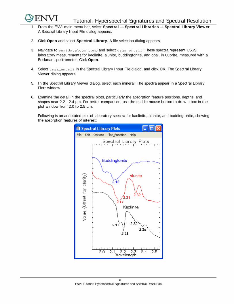
5. In the Spectral Library Viewer dialog, select each mineral. The spectra appear in a Spectral Library Plots window.

6. Examine the detail in the spectral plots, particularly the absorption feature positions, depths, and

shapes near 2.2 - 2.4 µm. For better comparison, use the middle mouse button to draw a box in the plot window from 2.0 to 2.5 µm.

Following is an annotated plot of laboratory spectra for kaolinite, alunite, and buddingtonite, showing the absorption features of interest:



View Landsat TM Image and Spectra The following plot shows region of interest (ROI) mean spectra for kaolinite, alunite, and buddingtonite. The small squares indicate the TM band 7 (2.21 µm) center point. The lines indicate the slope from TM band 5 (1.65 µm). The spectra appear very similar, and you cannot effectively discriminate between the three endmembers.

View TM Mean Kaolinite and Alunite Image Spectra 1. From the ENVI main menu bar, select Window → Start New Plot Window. A blank ENVI Plot

Window appears.

2. From the ENVI Plot Window menu bar, select File → Input Data → ASCII. A file selection dialog appears.

3. Select cuptm_em.txt and click Open. An Input ASCII File dialog appears. Click OK to plot the mean

kaolinite and alunite spectra.

Compare Mean Spectra and Library Spectra Refer to these steps throughout the rest of the tutorial whenever you compare library spectra and ROI mean spectra from different sensors.

4. Right-click in the Spectral Library Plots window and select Plot Key.

5. Click and drag the Kaolinite and Alunite spectrum names from the Spectral Library Plots window to the ENVI Plot Window.

6. Right-click in the ENVI Plot Window and select Plot Key.



7. For easier comparison, select Edit → Data Parameters from the ENVI Plot Window menu bar, and change the Mean:Kaolinite and Mean:Alunite colors to match the colors of the corresponding library spectra.

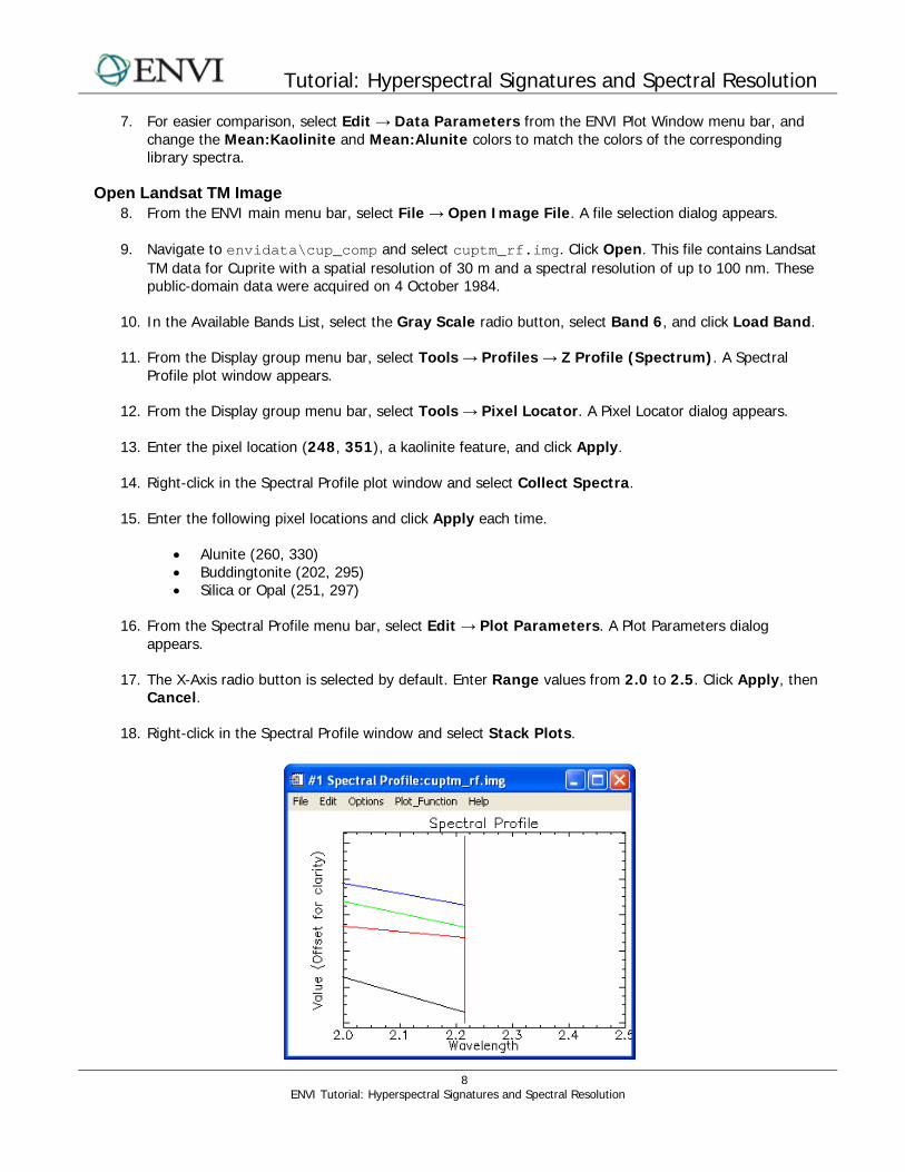
Open Landsat TM Image 8. From the ENVI main menu bar, select File → Open Image File. A file selection dialog appears. 9. Navigate to envidata\cup_comp and select cuptm_rf.img. Click Open. This file contains Landsat

TM data for Cuprite with a spatial resolution of 30 m and a spectral resolution of up to 100 nm. These public-domain data were acquired on 4 October 1984.

10. In the Available Bands List, select the Gray Scale radio button, select Band 6, and click Load Band.

11. From the Display group menu bar, select Tools → Profiles → Z Profile (Spectrum). A Spectral

Profile plot window appears.

12. From the Display group menu bar, select Tools → Pixel Locator. A Pixel Locator dialog appears.

13. Enter the pixel location (248, 351), a kaolinite feature, and click Apply.

14. Right-click in the Spectral Profile plot window and select Collect Spectra.

15. Enter the following pixel locations and click Apply each time.

• Alunite (260, 330) • Buddingtonite (202, 295) • Silica or Opal (251, 297)

16. From the Spectral Profile menu bar, select Edit → Plot Parameters. A Plot Parameters dialog

appears. 17. The X-Axis radio button is selected by default. Enter Range values from 2.0 to 2.5. Click Apply, then

Cancel.

18. Right-click in the Spectral Profile window and select Stack Plots.

8

ENVI Tutorial: Hyperspectral Signatures and Spectral Resolution

Tutorial: Hyperspectral Signatures and Spectral Resolution 19. Compare the apparent reflectance spectra to the library spectra, by dragging and dropping spectra

from the ENVI Plot Window into the Spectral Profile.

20. See Draw Conclusions on page 19, and answer some of the questions pertaining to Landsat TM data. 21. When you are finished, close the display group, ENVI Plot Window, and Spectral Profile. Keep the

Spectral Library Plots window open for the remaining exercises.

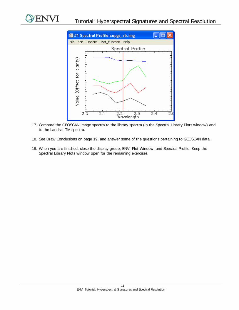
View GEOSCAN Image and Spectra The GEOSCAN MkII sensor, flown on a light aircraft during the late 1980s, was a commercial aircraft system that acquired up to 24 spectral channels selected from 46 available bands. GEOSCAN covered a spectral range from 0.45 to 12.0 µm using grating dispersive optics and three sets of linear array detectors (Lyon and Honey, 1989). GEOSCAN's high spatial resolution makes it suitable for detailed geologic mapping (Hook et al., 1991). A typical data acquisition for geology resulted in 10 bands in the visible/near infrared (VNIR, 0.52 - 0.96 µm), 8 bands in the shortwave infrared (SWIR, 2.04 - 2.35 µm), and thermal infrared (TIR, 8.64 - 11.28 µm) regions (Lyon and Honey, 1990). The relatively low number of spectral bands and low spectral resolution limit mineralogic mapping to a few groups of minerals in the absence of ground information. However, the strategic placement of the SWIR bands provides more mineralogic information than expected under such limited spectral resolution. The following plot shows ROI mean spectra for kaolinite, alunite, and buddingtonite. The spectra for these minerals appear quite different in the GEOSCAN data, even with the relatively widely spaced spectral bands.

View GEOSCAN Mean Kaolinite and Alunite Image Spectra 1. From the ENVI main menu bar, select Window → Start New Plot Window. A blank ENVI Plot

Window appears.





3. Select cupgs_em.txt and click Open. An Input ASCII File dialog appears. Click OK to plot the

kaolinite and alunite spectra in the ENVI Plot Window.

4. Compare these spectra to the USGS library spectra (in the Spectral Library Plots window) and to the spectra from the other sensors.

Open GEOSCAN Image 5. From the ENVI main menu bar, select File → Open Image File. A file selection dialog appears. 6. Navigate to envidata\cup_comp and select cupgs_sb.img. Click Open. This file contains

GEOSCAN imagery of Cuprite (collected in 1989), at approximately 60 nm spectral resolution with 44 nm sampling, converted to apparent reflectance using a Flat Field correction in ENVI.

7. To optionally view a color composite that enhances mineralogical differences, select the RGB Color

radio button, select Band 13, Band 15, and Band 18, and click Load RGB.









14. From the Spectral Profile menu bar, select Edit → Plot Parameters. A Plot Parameters dialog

appears. 15. The X-Axis radio button is selected by default. Enter Range values from 2.0 to 2.5. Click Apply, then

Cancel.



17. Compare the GEOSCAN image spectra to the library spectra (in the Spectral Library Plots window) and

to the Landsat TM spectra. 18. See Draw Conclusions on page 19, and answer some of the questions pertaining to GEOSCAN data.

19. When you are finished, close the display group, ENVI Plot Window, and Spectral Profile. Keep the




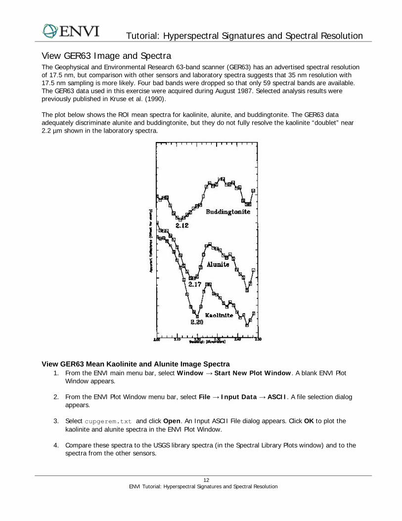
View GER63 Image and Spectra The Geophysical and Environmental Research 63-band scanner (GER63) has an advertised spectral resolution of 17.5 nm, but comparison with other sensors and laboratory spectra suggests that 35 nm resolution with 17.5 nm sampling is more likely. Four bad bands were dropped so that only 59 spectral bands are available. The GER63 data used in this exercise were acquired during August 1987. Selected analysis results were previously published in Kruse et al. (1990). The plot below shows the ROI mean spectra for kaolinite, alunite, and buddingtonite. The GER63 data adequately discriminate alunite and buddingtonite, but they do not fully resolve the kaolinite “doublet” near 2.2 µm shown in the laboratory spectra.

View GER63 Mean Kaolinite and Alunite Image Spectra 1. From the ENVI main menu bar, select Window → Start New Plot Window. A blank ENVI Plot

Window appears.


3. Select cupgerem.txt and click Open. An Input ASCII File dialog appears. Click OK to plot the

kaolinite and alunite spectra in the ENVI Plot Window.



Tutorial: Hyperspectral Signatures and Spectral Resolution Open GER63 Image

5. From the ENVI main menu bar, select File → Open Image File. A file selection dialog appears. 6. Navigate to envidata\cup_comp and select cupgersb.img. Click Open.











14. From the Spectral Profile menu bar, select Edit → Plot Parameters. A Plot Parameters dialog appears.

15. The X-Axis radio button is selected by default. Enter Range values from 2.0 to 2.5. Click Apply, then

Cancel.


17. Compare the GER63 image spectra to the library spectra (in the Spectral Library Plots window) and to spectra from the other sensors.


Tutorial: Hyperspectral Signatures and Spectral Resolution 18. See Draw Conclusions on page 19, and answer some of the questions pertaining to GER63 data.



View HyMap Image and Spectra HyMap is a state-of-the-art, aircraft-mounted, hyperspectral sensor developed by Integrated Spectronics, Sydney, Australia, and operated by HyVista Corporation. HyMap provides unprecedented spatial, spectral and radiometric resolution (Cocks et al., 1998). The system has a whiskbroom scanner utilizing diffraction gratings and four 32-element detector arrays to provide 126 spectral channels covering the 0.44 - 2.5 µm range over a 512-pixel swath. Spectral resolution varies from 10 - 20 nm with 3 – 10 m spatial resolution and a signal-to-noise ratio over 1000:1. The HyMap data described here were acquired on September 11, 1999. Selected analysis results were published in Kruse et al. (1999). The plot below shows ROI mean spectra for kaolinite, alunite, and buddingtonite.

View HyMap Mean Kaolinite and Alunite Image Spectra 1. From the ENVI main menu bar, select Window → Start New Plot Window. A blank ENVI Plot

Window appears.





3. Navigate to envidata\cup99hym and select cup99hy_em.txt. Click Open. An Input ASCII File dialog appears. Click OK to plot the kaolinite and alunite spectra in the ENVI Plot Window.

4. Compare these spectra to the USGS library spectra (in the Spectral Library Plots window) and to the

spectra from the other sensors.

Open HyMap Image 5. From the ENVI main menu bar, select File → Open Image File. A file selection dialog appears. 6. Navigate to envidata\cup99hym and select cup99hy.eff. Click Open. This file contains HyMap

reflectance data for Cuprite, produced by running calibrated radiance data through the ATREM atmospheric correction model, followed by EFFORT polishing (Kruse et al., 1999). The data are rotated 180 degrees from north, so north is at the bottom of the image.













Cancel.


17. Compare the HyMap image spectra to the library spectra (in the Spectral Library Plots window) and to spectra from the other sensors.

18. See Draw Conclusions on page 19, and answer some of the questions pertaining to HyMap data.


Spectral Library Plots window open for the remaining exercise.


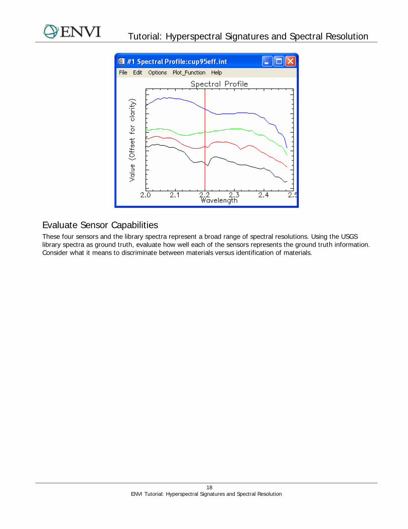
View AVIRIS Image and Spectra AVIRIS data have approximately 10 nm spectral resolution and 20 m spatial resolution. The AVIRIS data used in this exercise were acquired during July 1995 as part of an AVIRIS Group Shoot (Kruse and Huntington, 1996). Data were corrected to reflectance by running calibrated radiance data through the ATREM atmospheric correction model, followed by EFFORT polishing. The following plot shows the ROI mean spectra for kaolinite, alunite, and buddingtonite. Compare these to the library spectra and note the high quality and nearly identical signatures.

16

ENVI Tutorial: Hyperspectral Signatures and Spectral Resolution



View AVIRIS Mean Kaolinite and Alunite Image Spectra 1. From the ENVI main menu bar, select Window → Start New Plot Window. A blank ENVI Plot

Window appears.


3. Navigate to envidata\c95avsub and select cup95eff.txt. Click Open. An Input ASCII File dialog

appears. Click OK to plot the kaolinite and alunite spectra in the ENVI Plot Window.


Open AVIRIS Image 5. From the ENVI main menu bar, select File → Open Image File. A file selection dialog appears. 6. Navigate to envidata\c95avsub and select cup95eff.int. Click Open. A color composite of

bands 183, 193, and 207 automatically loads in a new display group.





10. Enter the pixel location (500, 581), which is a Kaolinite feature, and click Apply.






Cancel.


16. Compare the AVIRIS image spectra to the library spectra (in the Spectral Library Plots window) and to spectra from the other sensors.

17. See Draw Conclusions on page 19, and answer some of the questions pertaining to AVIRIS data.


Evaluate Sensor Capabilities These four sensors and the library spectra represent a broad range of spectral resolutions. Using the USGS library spectra as ground truth, evaluate how well each of the sensors represents the ground truth information. Consider what it means to discriminate between materials versus identification of materials.




Draw Conclusions 1. From the library spectra, what is the minimum spacing of absorption features in the 2.0 - 2.5 µm

range? 2. The TM data dramatically undersample the 2.0 - 2.5 µm range, as only TM band 7 is available. What

evidence do you see for absorption features in this range? What differences are apparent in the TM spectra of minerals with absorption features in this range?

3. The GEOSCAN data also undersample the 2.0 - 2.5 µm range, however, the bands are strategically

placed. What differences do you see between the GEOSCAN spectra for the different minerals? Could some of the bands have been placed differently to provide better mapping of specific minerals?

4. The GER63 data provide improved spectral resolution over the GEOSCAN data, and you can observe

individual features. The advertised spectral resolution of the GER63 between 2.0 - 2.5 µm is 17.5 nm. Examine the GER63 kaolinite spectrum and defend or refute this specification. Do the more closely spaced spectral bands of the GER63 sensor provide a significant advantage over the GEOSCAN data in mapping and identifying these reference minerals?

5. What are the main differences between mineral spectra at Cuprite caused by the change from 10 nm

spectral resolution (AVIRIS) to 17 nm spectral resolution (HyMap)?

6. The AVIRIS data provide the best spectral resolution of the sensors examined here. How do the AVIRIS and laboratory spectra compare? What are the major similarities and differences? What factors affect the comparison of the two data types?

7. Examine all of the images and spectra. What role does spatial resolution play in the comparison?

8. Based on the library spectra, provide sensor spectral and spatial resolution design specifications as

well as recommendations on placement of spectral bands for mineral mapping. Examine the trade-offs between continuous high-spectral resolution bands and strategically placed, lower-resolution bands.



References Abrams, M. J., R. P. Ashley, L. C. Rowan, A. F. H. Goetz, and A. B. Kahle, 1978, Mapping of hydrothermal alteration in the Cuprite Mining District, Nevada using aircraft scanner images for the spectral region 0.46 - 2.36 µm: Geology, v. 5., p. 173 - 718. Abrams, M., and S. J. Hook, 1995, Simulated ASTER data for Geologic Studies: IEEE Transactions on Geoscience and Remote Sensing, v. 33, no. 3, p. 692 - 699. Chrien, T. G., R. O. Green, and M. L. Eastwood, 1990, Accuracy of the spectral and radiometric laboratory calibration of the Airborne Visible/Infrared Imaging Spectrometer: in Proceedings The International Society for Optical Engineering (SPIE), v. 1298, p. 37-49. Clark, R. N., T. V. V. King, M. Klejwa, and G. A. Swayze, 1990, High spectral resolution spectroscopy of minerals: Journal of Geophysical Research, v. 95, no., B8, p. 12653 - 12680. Clark, R. N., G. A. Swayze, A. Gallagher, T. V. V. King, and W. M. Calvin, 1993, The U. S. Geological Survey Digital Spectral Library: Version 1: 0.2 to 3.0 µm: U. S. Geological Survey, Open File Report 93-592, 1340 p. Cocks T., R. Jenssen, A. Stewart, I. Wilson, and T. Shields, 1998, The HyMap Airborne Hyperspectral Sensor: The System, Calibration and Performance. Proc. 1st EARSeL Workshop on Imaging Spectroscopy (M. Schaepman, D. Schlopfer, and K.I. Itten, Eds.), 6-8 October 1998, Zurich, EARSeL, Paris, p. 37-43. CSES, 1992, Atmosphere REMoval Program (ATREM) User’s Guide, Version 1.1, Center for the Study of Earth from Space, Boulder, Colorado, 24 p. Goetz, A. F. H., and B. Kindel, 1996, Understanding unmixed AVIRIS images in Cuprite, NV using coincident HYDICE data: in Summaries of the Sixth Annual JPL Airborne Earth Science Workshop, March 4-8, 1996, v. 1 (Preliminary). Goetz, A. F. H., and L. C. Rowan, 1981, Geologic Remote Sensing: Science, v. 211, p. 781 - 791. Goetz, A. F. H., B. N. Rock, and L. C. Rowan, 1983, Remote Sensing for Exploration: An Overview: Economic Geology, v. 78, no. 4, p. 573 - 590. Goetz, A. F. H., G. Vane, J. E. Solomon, and B. N. Rock, 1985, Imaging spectrometry for earth remote sensing: Science, v. 228, p. 1147 - 1153. Green, R. O., J. E. Conel, J. Margolis, C. Chovit, and J. Faust, 1996, In-flight calibration and validation of the Airborne Visible/Infrared Imaging Spectrometer (AVIRIS): in Summaries of the Sixth Annual JPL Airborne Geoscience Workshop, 4-8 March 1996, Jet Propulsion Laboratory, Pasadena, CA, v. 1, (Preliminary). Hook, S. J., C. D. Elvidge, M. Rast, and H. Watanabe, 1991, An evaluation of short-waveinfrared (SWIR) data from the AVIRIS and GEOSCAN instruments for mineralogic mapping at Cuprite, Nevada: Geophysics, v. 56, no. 9, p. 1432 - 1440. Kruse, F. A., 1988, Use of Airborne Imaging Spectrometer data to map minerals associated with hydrothermally altered rocks in the northern Grapevine Mountains, Nevada and California: Remote Sensing of Environment, V. 24, No. 1, p. 31-51. Kruse, F. A., and J. H. Huntington, 1996, The 1995 Geology AVIRIS Group Shoot: in Summaries of the Sixth Annual JPL Airborne Earth Science Workshop, March 4 - 8, 1996 Volume 1, AVIRIS Workshop, (Preliminary).



Kruse, F. A., K. S. Kierein-Young, and J. W. Boardman, 1990, Mineral mapping at Cuprite, Nevada with a 63 channel imaging spectrometer: Photogrammetric Engineering and Remote Sensing, v. 56, no. 1, p. 83-92. Kruse, F. A., J. W. Boardman, A. B. Lefkoff, J. M. Young, K. S. Kierein-Young, T. D. Cocks, R. Jenssen, and P. A. Cocks, 2000, HyMap: An Australian Hyperspectral Sensor Solving Global Problems - Results from USA HyMap Data Acquisitions: in Proceedings of the 10th Australasian Remote Sensing and Photogrammetry Conference, Adelaide, Australia, 21-25 August 2000 (In Press). Lyon, R. J. P., and F. R. Honey, 1989, spectral signature extraction from airborne imagery using the Geoscan MkII advanced airborne scanner in the Leonora, Western Australia Gold District: in IGARSS-89/12th Canadian Symposium on Remote Sensing, v. 5, p. 2925 - 2930. Lyon, R.J. P., and F. R. Honey, 1990, Thermal Infrared imagery from the Geoscan Mark II scanner of the Ludwig Skarn, Yerington, NV: in Proceedings of the Second Thermal Infrared Multispectral Scanner (TIMS) Workshop. Paylor, E. D., M. J. Abrams, J. E. Conel, A. B. Kahle, and H. R. Lang, 1985, Performance evaluation and geologic utility of Landsat-4 Thematic Mapper Data: JPL Publication 85-66, Jet Propulsion Laboratory, Pasadena, CA, 68 p. Pease, C. B., 1990, Satellite imaging instruments: Principles, Technologies, and Operational Systems: Ellis Horwid, N.Y., 336 p. Porter, W. M., and H. E. Enmark, 1987, System overview of the Airborne Visible/Infrared Imaging Spectrometer (AVIRIS), in Proceedings, Society of Photo-Optical Instrumentation Engineers (SPIE), v. 834, p. 22-31. Swayze, Gregg, 1997, The hydrothermal and structural history of the Cuprite Mining District, Southwestern Nevada: an integrated geological and geophysical approach: Unpublished Ph.D. Dissertation, University of Colorado, Boulder.

ENVI Tutorial: Hyperspectral Signatures and Spectral ... · Tutorial: Hyperspectral Signatures and...

Documents

Transcript of ENVI Tutorial: Hyperspectral Signatures and Spectral ... · Tutorial: Hyperspectral Signatures and...