Regression discontinuity designs: A guide to...

ARTICLE IN PRESS

0304-4076/$ - se

doi:10.1016/j.je

�CorrespondE-mail addr

Please cite thi

(2007), doi:10

Journal of Econometrics ] (]]]]) ]]]–]]]

www.elsevier.com/locate/jeconom

Regression discontinuity designs: A guide to practice

Guido W. Imbensa, Thomas Lemieuxb,�

aDepartment of Economics, Harvard University and NBER, M-24 Littauer Center, Cambridge, MA 02138, USAbDepartment of Economics, University of British Columbia and NBER, 997-1873 East Mall, Vancouver, BC, V6T 1Z1, Canada

Abstract

In regression discontinuity (RD) designs for evaluating causal effects of interventions, assignment to a treatment is

determined at least partly by the value of an observed covariate lying on either side of a fixed threshold. These designs were

first introduced in the evaluation literature by Thistlewaite and Campbell [1960. Regression-discontinuity analysis: an

alternative to the ex-post Facto experiment. Journal of Educational Psychology 51, 309–317] With the exception of a few

unpublished theoretical papers, these methods did not attract much attention in the economics literature until recently.

Starting in the late 1990s, there has been a large number of studies in economics applying and extending RD methods. In

this paper we review some of the practical and theoretical issues in implementation of RD methods.

r 2007 Elsevier B.V. All rights reserved.

JEL classification: C14; C21

Keywords: Regression discontinuity; Treatment effects; Nonparametric estimation

1. Introduction

Since the late 1990s there has been a large number of studies in economics applying and extendingregression discontinuity (RD) methods, including Van Der Klaauw (2002), Black (1999), Angrist and Lavy(1999), Lee (2007), Chay and Greenstone (2005), DiNardo and Lee (2004), Chay et al. (2005), and Card et al.(2006). Key theoretical and conceptual contributions include the interpretation of estimates for fuzzyregression discontinuity (FRD) designs allowing for general heterogeneity of treatment effects (Hahn et al.,2001, HTV from hereon), adaptive estimation methods (Sun, 2005), specific methods for choosing bandwidths(Ludwig and Miller, 2005), and various tests for discontinuities in means and distributions of non-affectedvariables (Lee, 2007; McCrary, 2007).

In this paper, we review some of the practical issues in implementation of RD methods. There is relativelylittle novel in this discussion. Our general goal is instead to address practical issues in implementing RDdesigns and review some of the new theoretical developments.

After reviewing some basic concepts in Section 2, the paper focuses on five specific issues in theimplementation of RD designs. In Section 3 we stress graphical analyses as powerful methods for illustrating

e front matter r 2007 Elsevier B.V. All rights reserved.

conom.2007.05.001

ing author. Tel.: +1604 822 2092; fax: +1 604 822 5915.

esses: [email protected] (G.W. Imbens), [email protected] (T. Lemieux).

s article as: Imbens, G.W., Lemieux, T., Regression discontinuity designs: A guide to practice, Journal of Econometrics

.1016/j.jeconom.2007.05.001

www.elsevier.com/locate/jeconom

dx.doi.org/10.1016/j.jeconom.2007.05.001

mailto:[email protected]

mailto:[email protected]


ARTICLE IN PRESSG.W. Imbens, T. Lemieux / Journal of Econometrics ] (]]]]) ]]]–]]]2

the design. In Section 4 we discuss estimation and suggest using local linear regression methods using only theobservations close to the discontinuity point. In Section 5 we propose choosing the bandwidth using cross-validation. In Section 6 we provide a simple plug-in estimator for the asymptotic variance and a secondestimator that exploits the link with instrumental variable methods derived by HTV. In Section 7 we discuss anumber of specification tests and sensitivity analyses based on tests for (a) discontinuities in the average valuesfor covariates, (b) discontinuities in the conditional density of the forcing variable, as suggested by McCrary,and (c) discontinuities in the average outcome at other values of the forcing variable.

2. Sharp and FRD designs

2.1. Basics

Our discussion will frame the RD design in the context of the modern literature on causal effects andtreatment effects, using the Rubin Causal Model (RCM) set up with potential outcomes (Rubin, 1974;Holland, 1986; Imbens and Rubin, 2007), rather than the regression framework that was originally used in thisliterature. For a general discussion of the RCM and its use in the economic literature, see the survey by Imbensand Wooldridge (2007).

In the basic setting for the RCM (and for the RD design), researchers are interested in the causal effect of abinary intervention or treatment. Units, which may be individuals, firms, countries, or other entities, are eitherexposed or not exposed to a treatment. The effect of the treatment is potentially heterogenous across units. LetY ið0Þ and Y ið1Þ denote the pair of potential outcomes for unit i: Y ið0Þ is the outcome without exposure to thetreatment and Y ið1Þ is the outcome given exposure to the treatment. Interest is in some comparison of Y ið0Þand Y ið1Þ. Typically, including in this discussion, we focus on differences Y ið1Þ � Y ið0Þ. The fundamentalproblem of causal inference is that we never observe the pair Y ið0Þ and Y ið1Þ together. We therefore typicallyfocus on average effects of the treatment, that is, averages of Y ið1Þ � Y ið0Þ over (sub)populations, rather thanon unit-level effects. For unit i we observe the outcome corresponding to the treatment received. Let W i 2

f0; 1g denote the treatment received, with W i ¼ 0 if unit i was not exposed to the treatment, and W i ¼ 1otherwise. The outcome observed can then be written as

Y i ¼ ð1�W iÞ � Y ið0Þ þW i � Y ið1Þ ¼Y ið0Þ if W i ¼ 0;

Y ið1Þ if W i ¼ 1:

(In addition to the assignment W i and the outcome Y i, we may observe a vector of covariates or pretreatmentvariables denoted by ðX i;ZiÞ, where X i is a scalar and Zi is an M-vector. A key characteristic of X i and Zi isthat they are known not to have been affected by the treatment. Both X i and Zi are covariates, with a specialrole played by X i in the RD design. For each unit we observe the quadruple ðY i;W i;X i;ZiÞ. We assume thatwe observe this quadruple for a random sample from some well-defined population.

The basic idea behind the RD design is that assignment to the treatment is determined, either completely orpartly, by the value of a predictor (the covariate X i) being on either side of a fixed threshold. This predictormay itself be associated with the potential outcomes, but this association is assumed to be smooth, and so anydiscontinuity of the conditional distribution (or of a feature of this conditional distribution such as theconditional expectation) of the outcome as a function of this covariate at the cutoff value is interpreted asevidence of a causal effect of the treatment.

The design often arises from administrative decisions, where the incentives for units to participate in aprogram are partly limited for reasons of resource constraints, and clear transparent rules rather thandiscretion by administrators are used for the allocation of these incentives. Examples of such settings abound.For example, Hahn et al. (1999) study the effect of an anti-discrimination law that only applies to firms with atleast 15 employees. In another example, Matsudaira (2007) studies the effect of a remedial summer schoolprogram that is mandatory for students who score less than some cutoff level on a test (see also Jacob andLefgren, 2004). Access to public goods such as libraries or museums is often eased by lower prices forindividuals depending on an age cutoff value (senior citizen discounts and discounts for children under someage limit). Similarly, eligibility for medical services through medicare is restricted by age (Card et al., 2004).

Please cite this article as: Imbens, G.W., Lemieux, T., Regression discontinuity designs: A guide to practice, Journal of Econometrics

(2007), doi:10.1016/j.jeconom.2007.05.001


ARTICLE IN PRESS

0 1 2 3 4 5 6 7 8 9 10

0

0.2

0.4

0.6

0.8

1

Fig. 1. Assignment probabilities (SRD).

0 1 2 3 4 5 6 7 8 9 10

0

1

2

3

4

5

Fig. 2. Potential and observed outcome regression functions.

G.W. Imbens, T. Lemieux / Journal of Econometrics ] (]]]]) ]]]–]]] 3

2.2. The sharp regression discontinuity design

It is useful to distinguish between two general settings, the sharp and the fuzzy regression discontinuity(SRD and FRD from hereon) designs (e.g., Trochim, 1984, 2001; HTV). In the SRD design the assignment W i

is a deterministic function of one of the covariates, the forcing (or treatment-determining) variable X 1:

W i ¼ 1fX iXcg.

All units with a covariate value of at least c are assigned to the treatment group (and participation ismandatory for these individuals), and all units with a covariate value less than c are assigned to the controlgroup (members of this group are not eligible for the treatment). In the SRD design we look at thediscontinuity in the conditional expectation of the outcome given the covariate to uncover an average causaleffect of the treatment:

limx#c

E½Y ijX i ¼ x� � limx"c

E½Y ijX i ¼ x�,

which is interpreted as the average causal effect of the treatment at the discontinuity point

tSRD ¼ E½Y ið1Þ � Y ið0ÞjX i ¼ c�. (2.1)

Figs. 1 and 2 illustrate the identification strategy in the SRD setup. Based on artificial population values, wepresent in Fig. 1 the conditional probability of receiving the treatment, PrðW ¼ 1jX ¼ xÞ against the covariatex. At x ¼ 6 the probability jumps from 0 to 1. In Fig. 2, three conditional expectations are plotted. The twocontinuous lines (partly dashed, partly solid) in the figure are the conditional expectations of the two potentialoutcomes given the covariate, mwðxÞ ¼ E½Y ðwÞjX ¼ x�, for w ¼ 0; 1. These two conditional expectations arecontinuous functions of the covariate. Note that we can only estimate m0ðxÞ for xoc and m1ðxÞ for xXc.

1Here we take X i to be a scalar. More generally, the assignment can be a function of a vector of covariates. Formally, we can write this

as the treatment indicator being an indicator for the vector X i being an element of a subset of the covariate space, or

W i ¼ 1fX i 2 X1g,

where X1 � X, and X is the covariate space.


(2007), doi:10.1016/j.jeconom.2007.05.001



In addition we plot the conditional expectation of the observed outcome

E½Y jX ¼ x� ¼ E½Y jW ¼ 0;X ¼ x� � PrðW ¼ 0jX ¼ xÞ

þ E½Y jW ¼ 1;X ¼ x� � PrðW ¼ 1jX ¼ xÞ

in Fig. 2, indicated by a solid line. Although the two conditional expectations of the potential outcomes mwðxÞ

are continuous, the conditional expectation of the observed outcome jumps at x ¼ c ¼ 6.Now let us discuss the interpretation of limx#c E½Y ijX i ¼ x� � limx"c E½Y ijX i ¼ x� as an average causal effect

in more detail. In the SRD design, the widely used unconfoundedness assumption (e.g., Rosenbaum andRubin, 1983; Imbens, 2004) underlying most matching-type estimators still holds:

Y ið0Þ;Y ið1Þ@W ijX i.

This assumption holds in a trivial manner, because conditional on the covariates there is no variation in thetreatment. However, this assumption cannot be exploited directly. The problem is that the second assumptionthat is typically used for matching-type approaches, the overlap assumption which requires that for all valuesof the covariates there are both treated and control units, or

0oPrðW i ¼ 1jX i ¼ xÞo1,

is fundamentally violated. In fact, for all values of x the probability of assignment is either 0 or 1, rather thanalways between 0 and 1 as required by the overlap assumption. As a result, there are no values of x withoverlap.

This implies there is an unavoidable need for extrapolation. However, in large samples the amount ofextrapolation required to make inferences is arbitrarily small, as we only need to infer the conditionalexpectation of Y ðwÞ given the covariates e away from where it can be estimated. To avoid non-trivialextrapolation we focus on the average treatment effect at X ¼ c:

tSRD ¼ E½Y ð1Þ � Y ð0ÞjX ¼ c� ¼ E½Y ð1ÞjX ¼ c� � E½Y ð0ÞjX ¼ c�. (2.2)

By design, there are no units with X i ¼ c for whom we observe Y ið0Þ. We therefore will exploit the fact that weobserve units with covariate values arbitrarily close to c.2 In order to justify this averaging we make asmoothness assumption. Typically this assumption is formulated in terms of conditional expectations.

Assumption 2.1. (Continuity of Conditional Regression Functions)

E½Y ð0ÞjX ¼ x� and E½Y ð1ÞjX ¼ x�,

are continuous in x.

More generally, one might want to assume that the conditional distribution function is smooth in thecovariate. Let F Y ðwÞjX ðyjxÞ ¼ PrðY ðwÞpyjX ¼ xÞ denote the conditional distribution function of Y ðwÞ givenX . Then the general version of the assumption is:

Assumption 2.2. (Continuity of Conditional Distribution Functions)

FY ð0ÞjX ðyjxÞ and F Y ð1ÞjX ðyjxÞ,

are continuous in x for all y.

Both these assumptions are stronger than required, as we will only use continuity at x ¼ c, but it is rare thatit is reasonable to assume continuity for one value of the covariate, but not at other values of the covariate.We therefore make the stronger assumption.

Under either assumption,

E½Y ð0ÞjX ¼ c� ¼ limx"c

E½Y ð0ÞjX ¼ x� ¼ limx"c

E½Y ð0ÞjW ¼ 0;X ¼ x� ¼ limx"c

E½Y jX ¼ x�

2Although in principle the first term in the difference in (2.2) would be straightforward to estimate if we actually observed individuals

with X i ¼ x, with continuous covariates we also need to estimate this term by averaging over units with covariate values close to c.


(2007), doi:10.1016/j.jeconom.2007.05.001


ARTICLE IN PRESSG.W. Imbens, T. Lemieux / Journal of Econometrics ] (]]]]) ]]]–]]] 5

and similarly,

E½Y ð1ÞjX ¼ c� ¼ limx#c

E½Y jX ¼ x�.

Thus, the average treatment effect at c, tSRD, satisfies

tSRD ¼ limx#c

E½Y jX ¼ x� � limx"c

E½Y jX ¼ x�.

The estimand is the difference of two regression functions at a point. Hence, if we try to estimate thisobject without parametric assumptions on the two regression functions, we do not obtain root-N consistentestimators. Instead we get consistent estimators that converge to their limits at slower, nonparametricrates.

As an example of an SRD design, consider the study of the effect of party affiliation of a congressman oncongressional voting outcomes by Lee (2007). See also Lee et al. (2004). The key idea is that electoral districtswhere the share of the vote for a Democrat in a particular election was just under 50% are on average similarin many relevant respects to districts where the share of the Democratic vote was just over 50%, but the smalldifference in votes leads to an immediate and big difference in the party affiliation of the elected representative.In this case, the party affiliation always jumps at 50%, making this an SRD design. Lee looks at theincumbency effect. He is interested in the probability of Democrats winning the subsequent election,comparing districts where the Democrats won the previous election with just over 50% of the popular votewith districts where the Democrats lost the previous election with just under 50% of the vote.

2.3. The FRD design

In the FRD design, the probability of receiving the treatment needs not change from 0 to 1 at the threshold.Instead, the design allows for a smaller jump in the probability of assignment to the treatment at the threshold:

limx#c

PrðW i ¼ 1jX i ¼ xÞa limx"c

PrðW i ¼ 1jX i ¼ xÞ,

without requiring the jump to equal 1. Such a situation can arise if incentives to participate in a programchange discontinuously at a threshold, without these incentives being powerful enough to move all units fromnonparticipation to participation. In this design we interpret the ratio of the jump in the regression of theoutcome on the covariate to the jump in the regression of the treatment indicator on the covariate as anaverage causal effect of the treatment. Formally, the estimand is

tFRD ¼limx#c E½Y jX ¼ x� � limx"c E½Y jX ¼ x�

limx#c E½W jX ¼ x� � limx"c E½W jX ¼ x�.

Let us first consider the interpretation of this ratio. HTV, in arguably the most important theoretical paperin the recent RD literature, exploit the instrumental variables connection to interpret the FRD design whenthe effect of the treatment varies by unit, as in Imbens and Angrist (1994).3 Let W iðxÞ be potential treatmentstatus given cutoff point x, for x in some small neighborhood around c. W iðxÞ is equal to 1 if unit i would takeor receive the treatment if the cutoff point was equal to x. This requires that the cutoff point is at least inprinciple manipulable. For example, if X is age, one could imagine changing the age that makes an individualeligible for the treatment from c to cþ �. Then it is useful to assume monotonicity (see HTV).

Assumption 2.3. W iðxÞ is non-increasing in x at x ¼ c.

Next, define compliance status. This concept is similar to the one used in instrumental variables settings(e.g., Angrist et al., 1996). A complier is a unit such that

limx#Xi

W iðxÞ ¼ 0 and limx"Xi

W iðxÞ ¼ 1.

3The close connection between FRD and instrumental variables models led researchers in a number of cases to interpret RD designs as

instrumental variables settings. See, for example, Angrist and Krueger (1991) and Imbens and Van Der Klaauw (1995). The main

advantage of thinking of these designs as RD designs is that it suggests the specification analyses from Section 7.


(2007), doi:10.1016/j.jeconom.2007.05.001



Compliers are units that would get the treatment if the cutoff were at X i or below, but that would not get thetreatment if the cutoff were higher than X i. To be specific, consider an example where individuals with a testscore less than c are encouraged for a remedial teaching program (Matsudaira, 2007). Interest is in the effect ofthe program on subsequent test scores. Compliers are individuals who would participate if encouraged (if thetest score is below the cutoff for encouragement), but not if not encouraged (if test score is above the cutoff forencouragement). Nevertakers are units with

limx#X i


W iðxÞ ¼ 0,

and alwaystakers are units with

limx#X i


W iðxÞ ¼ 1.

Then,

tFRD ¼limx#c E½Y jX ¼ x� � limx"c E½Y jX ¼ x�

limx#c E½W jX ¼ x� � limx"c E½W jX ¼ x�

¼ E½Y ið1Þ � Y ið0Þjunit i is a complier and X i ¼ c�.

The estimand is an average effect of the treatment, but only averaged for units with X i ¼ c (by RD), and onlyfor compliers (people who are affected by the threshold).

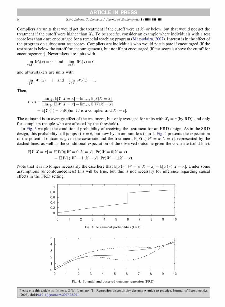
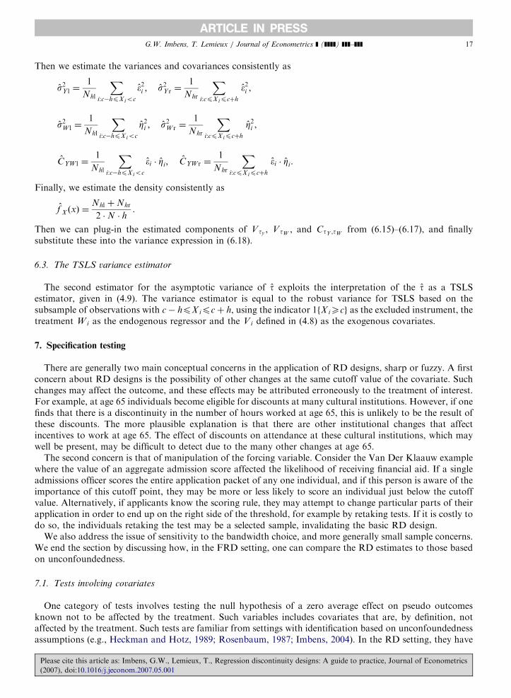
In Fig. 3 we plot the conditional probability of receiving the treatment for an FRD design. As in the SRDdesign, this probability still jumps at x ¼ 6, but now by an amount less than 1. Fig. 4 presents the expectationof the potential outcomes given the covariate and the treatment, E½Y ðwÞjW ¼ w;X ¼ x�, represented by thedashed lines, as well as the conditional expectation of the observed outcome given the covariate (solid line):

E½Y jX ¼ x� ¼ E½Y ð0ÞjW ¼ 0;X ¼ x� � PrðW ¼ 0jX ¼ xÞ

þ E½Y ð1ÞjW ¼ 1;X ¼ x� � PrðW ¼ 1jX ¼ xÞ.

Note that it is no longer necessarily the case here that E½Y ðwÞjW ¼ w;X ¼ x� ¼ E½Y ðwÞjX ¼ x�. Under someassumptions (unconfoundedness) this will be true, but this is not necessary for inference regarding causaleffects in the FRD setting.

0 1 2 3 4 5 6 7 8 9 10

0

0.2

0.4

0.6

0.8

1

Fig. 3. Assignment probabilities (FRD).

0 1 2 3 4 5 6 7 8 9 10

0

1

2

3

4

5

Fig. 4. Potential and observed outcome regression (FRD).


(2007), doi:10.1016/j.jeconom.2007.05.001



As an example of an FRD design, consider the study of the effect of financial aid on college attendance byVan Der Klaauw (2002). Van Der Klaauw looks at the effect of financial aid on acceptance on collegeadmissions. Here X i is a numerical score assigned to college applicants based on the objective part of theapplication information (SAT scores, grades) used to streamline the process of assigning financial aid offers.During the initial stages of the admission process, the applicants are divided into L groups based ondiscretized values of these scores. Let

Gi ¼

1 if 0pX ioc1;

2 if c1pX ioc2;

..

.

L if cL�1pX i;

8>>>><>>>>:denote the financial aid group. For simplicity, let us focus on the case with L ¼ 2, and a single cutoff point c.Having a score of just over c will put an applicant in a higher category and increase the chances of financial aiddiscontinuously compared to having a score of just below c. The outcome of interest in the Van Der Klaauwstudy is college attendance. In this case, the simple association between attendance and the financial aid offeris ambiguous. On the one hand, an aid offer makes the college more attractive to the potential student. This isthe causal effect of interest. On the other hand, a student who gets a generous financial aid offer is likely tohave better outside opportunities in the form of financial aid offers from other colleges. College aid isemphatically not a deterministic function of the financial aid categories, making this an FRD design. Othercomponents of the application that are not incorporated in the numerical score (such as the essay andrecommendation letters) undoubtedly play an important role. Nevertheless, there is a clear discontinuity in theprobability of receiving an offer of a larger financial aid package.

2.4. The FRD design and unconfoundedness

In the FRD setting, it is useful to contrast the RD approach with estimation of average causal effects underunconfoundedness. The unconfoundedness assumption (e.g., Rosenbaum and Rubin, 1983; Imbens, 2004)requires that

Y ð0Þ;Y ð1Þ@W jX .

If this assumption holds, then we can estimate the average effect of the treatment at X ¼ c as

E½Y ð1Þ � Y ð0ÞjX ¼ x� ¼ E½Y jW ¼ 1;X ¼ c� � E½Y jW ¼ 0;X ¼ c�.

This approach does not exploit the jump in the probability of assignment at the discontinuity point. Instead itassumes that differences between treated and control units with X i ¼ c are interpretable as average causal effects.

In contrast, the assumptions underlying an FRD analysis implies that comparing treated and control unitswith X i ¼ c is likely to be the wrong approach. Treated units with X i ¼ c include compliers and alwaystakers,and control units at X i ¼ c consist of nevertakers. Comparing these different types of units has no causalinterpretation under the FRD assumptions. Although, in principle, one cannot test the unconfoundednessassumption, one aspect of the problem makes this assumption fairly implausible. Unconfoundedness isfundamentally based on units being comparable if their covariates are similar. This is not an attractiveassumption in the current setting where the probability of receiving the treatment is discontinuous in thecovariate. Thus, units with similar values of the forcing variable (but on different sides of the threshold) mustbe different in some important way related to the receipt of treatment. Unless there is a substantive argumentthat this difference is immaterial for the comparison of the outcomes of interest, an analysis based onunconfoundedness is not attractive.

2.5. External validity

One important aspect of both the SRD and FRD designs is that they, at best, provide estimates of theaverage effect for a subpopulation, namely the subpopulation with covariate value equal to X i ¼ c. The FRD


(2007), doi:10.1016/j.jeconom.2007.05.001



design restricts the relevant subpopulation even further to that of compliers at this value of the covariate.Without strong assumptions justifying extrapolation to other subpopulations (e.g., homogeneity of thetreatment effect), the designs never allow the researcher to estimate the overall average effect of the treatment.In that sense the design has fundamentally only a limited degree of external validity, although the specificaverage effect that is identified may well be of special interest, for example in cases where the policy questionconcerns changing the location of the threshold. The advantage of RD designs compared to other non-experimental analyses that may have more external validity, such as those based on unconfoundedness is thatRD designs may have a relatively high degree of internal validity (in settings where they are applicable).

3. Graphical analyses

3.1. Introduction

Graphical analyses should be an integral part of any RD analysis. The nature of RD designs suggests thatthe effect of the treatment of interest can be measured by the value of the discontinuity in the expected value ofthe outcome at a particular point. Inspecting the estimated version of this conditional expectation is a simpleyet powerful way to visualize the identification strategy. Moreover, to assess the credibility of the RD strategy,it is useful to inspect two additional graphs for covariates and the density of the forcing variable. Theestimators we discuss later use more sophisticated methods for smoothing but these basic plots will conveymuch of the intuition. For strikingly clear examples of such plots, see Lee et al. (2004), Lalive (2007), and Lee(2007). Note that, in practice, the visual clarity of the plots is often improved by adding smoothed regressionlines based on polynomial regressions (or other flexible methods) estimated separately on the two sides of thecutoff point.

3.2. Outcomes by forcing variable

The first plot is a histogram-type estimate of the average value of the outcome for different values of theforcing variable, the estimated counterpart to the solid line in Figs. 2 and 4. For some binwidth h, and forsome number of bins K0 and K1 to the left and right of the cutoff value, respectively, construct bins ðbk; bkþ1�,for k ¼ 1; . . . ;K ¼ K0 þ K1, where

bk ¼ c� ðK0 � k þ 1Þ � h.

Then calculate the number of observations in each bin

Nk ¼XN

i¼1

1fbkoX ipbkþ1g

and the average outcome in the bin

Y k ¼1

Nk

�XN

i¼1

Y i � 1fbkoX ipbkþ1g.

The first plot of interest is that of the Y k, for k ¼ 1; . . . ;K against the mid point of the bins,~bk ¼ ðbk þ bkþ1Þ=2. The question is whether around the threshold c there is any evidence of a jump in theconditional mean of the outcome. The formal statistical analyses discussed below are essentially justsophisticated versions of this, and if the basic plot does not show any evidence of a discontinuity, there isrelatively little chance that the more sophisticated analyses will lead to robust and credible estimates withstatistically and substantially significant magnitudes. In addition to inspecting whether there is a jump at thisvalue of the covariate, one should inspect the graph to see whether there are any other jumps in the conditionalexpectation of Y given X that are comparable to, or larger than, the discontinuity at the cutoff value. If so,and if one cannot explain such jumps on substantive grounds, it would call into question the interpretation ofthe jump at the threshold as the causal effect of the treatment. In order to optimize the visual clarity it isimportant to calculate averages that are not smoothed over the cutoff point.


(2007), doi:10.1016/j.jeconom.2007.05.001



3.3. Covariates by forcing variable

The second set of plots compares average values of other covariates in the K bins. Specifically, let Zi be theM-vector of additional covariates, with mth element Zim. Then calculate

Zkm ¼1

Nk

�XN

i¼1

Zim � 1fbkoX ipbkþ1g.

The second plot of interest is that of the Zkm, for k ¼ 1; . . . ;K against the mid point of the bins, ~bk, for allm ¼ 1; . . . ;M. In the case of FRD designs, it is also particularly useful to plot the mean values of the treatmentvariable W i to make sure there is indeed a jump in the probability of treatment at the cutoff point (as in Fig. 3.Plotting other covariates is also useful for detecting possible specification problems (see Section 7.1) in thecase of either SRD or FRD designs.

3.4. The Density of the forcing variable

In the third graph, one should plot the number of observations in each bin, Nk, against the mid points ~bk.This plot can be used to inspect whether there is a discontinuity in the distribution of the forcing variable X atthe threshold. Such discontinuity would raise the question of whether the value of this covariate wasmanipulated by the individual agent, invalidating the design. For example, suppose that the forcing variable isa test score. If individuals know the threshold and have the option of retaking the test, individuals with testscores just below the threshold may do so, and invalidate the design. Such a situation would lead to adiscontinuity of the conditional density of the test score at the threshold, and thus be detectable in the kind ofplots described here. See Section 7.2 for more discussion of tests based on this idea.

4. Estimation: local linear regression

4.1. Nonparametric regression at the boundary

The practical estimation of the treatment effect t in both the SRD and FRD designs is largely a standardnonparametric regression problem (e.g., Pagan and Ullah, 1999; Hardle, 1990; Li and Racine, 2007).However, there are two unusual features. In this case we are interested in the regression function at a singlepoint, and in addition that single point is a boundary point. As a result, standard nonparametric kernelregression does not work very well. At boundary points, such estimators have a slower rate of convergencethan they do at interior points. Here we discuss a more attractive implementation suggested by HTV, amongothers. First define the conditional means

mlðxÞ ¼ limz"x

E½Y ð0ÞjX ¼ z� and mrðxÞ ¼ limz#x

E½Y ð1ÞjX ¼ z�.

The estimand in the SRD design is, in terms of these regression functions,

tSRD ¼ mrðcÞ � mlðcÞ.

A natural approach is to use standard nonparametric regression methods for estimation of mlðxÞ and mrðxÞ.Suppose we use a kernel KðuÞ, with

RKðuÞdu ¼ 1. Then the regression functions at x can be estimated as

mlðxÞ ¼

Pi:Xioc Y i � KððX i � xÞ=hÞP

i:X ioc KððX i � xÞ=hÞand mrðxÞ ¼

Pi:XiXc Y i � KððX i � xÞ=hÞP

i:X iXc KððX i � xÞ=hÞ,

where h is the bandwidth.The estimator for the object of interest is then

tSRD ¼ mrðxÞ � mlðxÞ ¼

Pi:X iXc Y i � KððX i � xÞ=hÞP

i:X iXc KððX i � xÞ=hÞ�

Pi:X ioc Y i � KððX i � xÞ=hÞP

i:X ioc KððX i � xÞ=hÞ.


(2007), doi:10.1016/j.jeconom.2007.05.001



In order to see the nature of this estimator for the SRD case, it is useful to focus on a special case. Suppose weuse a rectangular kernel, e.g., KðuÞ ¼ 1

2 for �1ouo1, and 0 elsewhere. Then the estimator can be written as

tSRD ¼

PNi¼1 Y i � 1fcpX ipcþ hgPN

i¼1 1fcpX ipcþ hg�

PNi¼1 Y i � 1fc� hpX iocgPN

i¼1 1fc� hpX iocg

¼ Y hr � Y hl,

the difference between the average outcomes for observations within a distance h of the cutoff point on theright and left of the cutoff, respectively. Nhr and Nhl denote the number of observations with X i 2 ½c; cþ h�

and X i 2 ½c� h; cÞ, respectively. This estimator can be interpreted as first discarding all observations with avalue of X i more than h away from the discontinuity point c, and then simply differencing the averageoutcomes by treatment status in the remaining sample.

This simple nonparametric estimator is in general not very attractive, as pointed out by HTV and Porter(2003). Let us look at the approximate bias of this estimator through the probability limit of the estimator forfixed bandwidth. The probability limit of mrðcÞ, using the rectangular kernel, is

plim½mrðcÞ� ¼

R cþh

cmðxÞf ðxÞdxR cþh

cf ðxÞdx

¼ mrðcÞ þ limx#c

qqx

mðxÞ �h

2þOðh2

Þ.

Combined with the corresponding calculation for the control group, we obtain the bias

plim½mrðcÞ � mlðcÞ� � mrðcÞ � mlðcÞ ¼h

2� lim

x#c

qqx

mðxÞ þ limx"c

qqx

mðxÞ� �

þOðh2Þ.

Hence the bias is linear in the bandwidth h, whereas when we nonparametrically estimate a regression functionin the interior of the support we typically get a bias of order h2.

Note that we typically do expect the regression function to have a non-zero derivative, even in cases where thetreatment has no effect. In many applications the eligibility criterion is based on a covariate that does have somecorrelation with the outcome, so that, for example, those with poorest prospects in the absence of the programare in the eligible group. Hence it is likely that the bias for the simple kernel estimator is relatively high.

One practical solution to the high order of the bias is to use a local linear regression (e.g., Fan and Gijbels,1996). An alternative is to use series regression or sieve methods. Such methods could be implemented in thecurrent setting by adding higher-order terms to the regression function. For example, Lee et al. (2004) includefourth-order polynomials in the covariate to the regression function. The formal properties of such methodsare equally attractive to those of kernel type methods. The main concern is that they are more sensitive tooutcome values for observations far away from the cutoff point. Kernel methods using kernels with compactsupport rule out any sensitivity to such observations, and given the nature of RD designs this can be anattractive feature. Certainly, it would be a concern if results depended in an important way on usingobservations far away from the cutoff value. In addition, global methods put effort into estimating theregression functions in areas (far away from the discontinuity point) that are of no interest in the currentsetting.

4.2. Local linear regression

Here we discuss local linear regression. See for a general discussion Fan and Gijbels (1996). Instead oflocally fitting a constant function, we can fit linear regression functions to the observations within a distance h

on either side of the discontinuity point

minal:bl

Xi:c�hoXioc

ðY i � al � bl � ðX i � cÞÞ2,

and

minar:br

Xi:cpX iocþh

ðY i � ar � br � ðX i � cÞÞ2.


(2007), doi:10.1016/j.jeconom.2007.05.001



The value of mlðcÞ is then estimated asdmlðcÞ ¼ al þ bl � ðc� cÞ ¼ al,

and the value of mrðcÞ is then estimated asdmrðcÞ ¼ ar þ br � ðc� cÞ ¼ ar.

Given these estimates, the average treatment effect is estimated as

tSRD ¼ ar � al.

Alternatively one can estimate the average effect directly in a single regression, by solving

mina;b;t;g

XN

i¼1

1fc� hpX ipcþ hg � ðY i � a� b � ðX i � cÞ � t �W i � g � ðX i � cÞ �W iÞ2,

which will numerically yield the same estimate of tSRD.An alternative is to impose the restriction that the slope coefficients are the same on both sides of the

discontinuity point, or limx#c ðq=qxÞmðxÞ ¼ limx"c ðq=qxÞmðxÞ. This can be imposed by requiring that bl ¼ br.Although it may be reasonable to expect the slope coefficients for the covariate to be similar on both sides ofthe discontinuity point, this procedure also has some disadvantages. Specifically, by imposing this restrictionone allows for observations on Y ð1Þ from the right of the discontinuity point to affect estimates of E½Y ð0ÞjX ¼c� and, similarly, for observations on Y ð0Þ from the left of discontinuity point to affect estimates ofE½Y ð1ÞjX ¼ c�. In practice, one might wish to have the estimates of E½Y ð0ÞjX ¼ c� based solely on observationson Y ð0Þ, and not depend on observations on Y ð1Þ, and vice versa.

We can make the nonparametric regression more sophisticated by using weights that decrease smoothly asthe distance to the cutoff point increases, instead of the 0/1 weights based on the rectangular kernel. However,even in this simple case the asymptotic bias can be shown to be of order h2, and the more sophisticated kernelsrarely make much difference. Furthermore, if using different weights from a more sophisticated kernel doesmake a difference, it likely suggests that the results are highly sensitive to the choice of bandwidth. So the onlycase where more sophisticated kernels may make a difference is when the estimates are not very credibleanyway because of too much sensitivity to the choice of bandwidth. From a practical point of view, one mayjust focus on the simple rectangular kernel, but verify the robustness of the results to different choices ofbandwidth.

For inference we can use standard least squares methods. Under appropriate conditions on the rate at whichthe bandwidth goes to 0 as the sample size increases, the resulting estimates will be asymptotically normallydistributed, and the (robust) standard errors from least squares theory will be justified. Using the results fromHTV, the optimal bandwidth is h / N�1=5. Under this sequence of bandwidths the asymptotic distribution ofthe estimator t will have a non-zero bias. If one does some undersmoothing, by requiring that h / N�d with1=5odo2=5, then the asymptotic bias disappears and standard least square variance estimators will lead tovalid confidence intervals. See Section 6 for more details.

4.3. Covariates

Often there are additional covariates available in addition to the forcing covariate that is the basis of theassignment mechanism. These covariates can be used to eliminate small sample biases present in the basicspecification, and improve the precision. In addition, they can be useful for evaluating the plausibility of theidentification strategy, as discussed in Section 7.1. Let the additional vector of covariates be denoted by Zi.We make three observations on the role of these additional covariates.

The first and most important point is that the presence of these covariates rarely changes the identificationstrategy. Typically, the conditional distribution of the covariates Z given X is continuous at x ¼ c. In fact, aswe discuss in Section 7, one may wish to test for discontinuities at that value of x in order to assess theplausibility of the identification strategy. If such discontinuities in other covariates are found, the justificationof the identification strategy may be questionable. If the conditional distribution of Z given X is continuous at


(2007), doi:10.1016/j.jeconom.2007.05.001



x ¼ c, then including Z in the regression

mina;b;t;d

XN

i¼1

1fc� hpX ipcþ hg � ðY i � a� b � ðX i � cÞ

� t �W i � g � ðX i � cÞ �W i � d0ZiÞ2,

will have little effect on the expected value of the estimator for t, since conditional on X being close to c, theadditional covariates Z are independent of W .

The second point is that even though the presence of Z in the regression does not affect any bias when X isvery close to c, in practice we often include observations with values of X not too close to c. In that case,including additional covariates may eliminate some bias that is the result of the inclusion of these additionalobservations.

Third, the presence of the covariates can improve precision if Z is correlated with the potential outcomes.This is the standard argument, which also supports the inclusion of covariates in analyses of randomizedexperiments. In practice the variance reduction will be relatively small unless the contribution to the R2 fromthe additional regressors is substantial.

4.4. Estimation for the FRD design

In the FRD design, we need to estimate the ratio of two differences. The estimation issues we discussedearlier in the case of the SRD arise now for both differences. In particular, there are substantial biases ifwe do simple kernel regressions. Instead, it is again likely to be better to use local linear regression. We use auniform kernel, with the same bandwidth for estimation of the discontinuity in the outcome and treatmentregressions.

First, consider local linear regression for the outcome, on both sides of the discontinuity point. Let

ðayl; bylÞ ¼ arg minayl;byl

Xi:c�hpXioc

ðY i � ayl � byl � ðX i � cÞÞ2, (4.3)

ðayr; byrÞ ¼ arg minayr;byr

Xi:cpXipcþh

ðY i � ayr � byr � ðX i � cÞÞ2. (4.4)

The magnitude of the discontinuity in the outcome regression is then estimated as

ty ¼ ayr � ayl.

Second, consider the two local linear regression for the treatment indicator:

ðawl; bwlÞ ¼ arg minawl;bwl

Xi:c�hpX ioc

ðW i � awl � bwl � ðX i � cÞÞ2, (4.5)

ðawr; bwrÞ ¼ arg minawr;bwr

Xi:cpXipcþh

ðY i � awr � bwr � ðX i � cÞÞ2. (4.6)

The magnitude of the discontinuity in the treatment regression is then estimated as

tw ¼ awr � awl.

Finally, we estimate the effect of interest as the ratio of the two discontinuities:

tFRD ¼ty

tw

¼ayr � ayl

awr � awl. (4.7)

Because of the specific implementation we use here, with a uniform kernel, and the same bandwidth forestimation of the denominator and the numerator, we can characterize the estimator for t as a two-stage leastsquares (TSLS) estimator. HTV were the first to note this equality, in the setting with standard kernel


(2007), doi:10.1016/j.jeconom.2007.05.001



regression and no additional covariates. It is a simple extension to show that the equality still holds when weuse local linear regression and include additional regressors. Define

Vi ¼

1

1fX iocg � ðX i � cÞ

1fX iXcg � ðX i � cÞ

0B@1CA and d ¼

ayl

byl

byr

0BBB@1CCCA. (4.8)

Then we can write

Y i ¼ d0V i þ t �W i þ ei. (4.9)

Estimating t based on the regression function (4.9) by TSLS methods, with the indicator 1fX iXcg as theexcluded instrument and V i as the set of exogenous variables is numerically identical to tFRD as given in (4.7).

5. Bandwidth selection

An important issue in practice is the selection of the smoothing parameter, the binwidth h. In general thereare two approaches to choose bandwidths. A first approach consists of characterizing the optimal bandwidthin terms of the unknown joint distribution of all variables. The relevant components of this distribution canthen be estimated, and plugged into the optimal bandwidth function. The second approach, on which we focushere, is based on a cross-validation procedure. The specific methods discussed here are similar to thosedeveloped by Ludwig and Miller (2005, 2007). In particular, their proposals, like ours, are aimed specifically atestimating the regression function at the boundary. Initially we focus on the SRD case, and in Section 5.2 weextend the recommendations to the FRD setting.

To set up the bandwidth choice problem we generalize the notation slightly. In the SRD setting we areinterested in

tSRD ¼ limx#c

mðxÞ � limx"c

mðxÞ.

We estimate the two terms as

dlimx#c

mðxÞ ¼ arðcÞ

and

dlimx"c

mðxÞ ¼ alðcÞ,

where alðxÞ and blðxÞ solve

ðalðxÞ; blðxÞÞ ¼ argmina;b

Xjjx�hoX jox

ðY j � a� b � ðX j � xÞÞ2. (5.10)

and arðxÞ and brðxÞ solve

ðarðxÞ; brðxÞÞ ¼ argmina;b

XjjxoXjoxþh

ðY j � a� b � ðX j � xÞÞ2. (5.11)

Let us focus first on estimating limx#c mðxÞ. For estimation of this limit we are interested in the bandwidth h

that minimizes

Qrðx; hÞ ¼ E limz#x

mðzÞ � arðxÞ� �2" #

,


(2007), doi:10.1016/j.jeconom.2007.05.001



at x ¼ c. In principle this could be different from the bandwidth that minimizes the corresponding criterion onthe left-hand side,

Qlðx; hÞ ¼ E limz"x

mðzÞ � alðxÞ� �2" #

,

at x ¼ c. However, we will focus on a single bandwidth for both sides of the threshold, and therefore focus onminimizing

Qðc; hÞ ¼1

2� ðQlðc; hÞ þQrðc; hÞÞ

¼1

2� E lim

x"cmðxÞ � alðcÞ

� �2" #

þ E limx#c

mðxÞ � arðcÞ� �2" # !

.

We now discuss two methods for choosing the bandwidth.

5.1. Bandwidth selection for the SRD design

For a given binwidth h, let the estimated regression function at x be

mðxÞ ¼alðxÞ if xoc;

arðxÞ if xXc;

(

where alðxÞ, blðxÞ, arðxÞ, and brðxÞ solve (5.10) and (5.11). Note that in order to mimic the fact that we areinterested in estimation at the boundary, we only use the observations on one side of x in order to estimate theregression function at x, rather than the observations on both sides of x, that is, observations withx� hoX joxþ h. In addition, the strict inequality in the definition implies that mðxÞ evaluated at x ¼ X i doesnot depend on Y i.

Now define the cross-validation criterion as

CVY ðhÞ ¼1

N

XN

i¼1

ðY i � mðX iÞÞ2 (5.12)

with the corresponding cross-validation choice for the binwidth

hoptCV ¼ arg min

hCVY ðhÞ.

The expected value of this cross-validation function is, ignoring the term that does not involve h, equal toE½CVY ðhÞ� ¼ C þ E½QðX ; hÞ� ¼ C þ

RQðx; hÞf X dx. Although the modification to estimate the regression

using one-sided kernels mimics more closely the estimand of interest, this is still not quite what we areinterested in. Ultimately, we are solely interested in estimating the regression function in the neighborhood ofa single point, the threshold c, and thus in minimizing Qðc; hÞ, rather than

Rx

Qðx; hÞf X ðxÞdx. If there are quitea few observations in the tails of the distribution, minimizing the criterion in (5.12) may lead to larger binsthan is optimal for estimating the regression function around x ¼ c, if c is in the center of the distribution. Wemay therefore wish to minimize the cross-validation criterion after first discarding observations from the tails.Let qX ;d;l be the d quantile of the empirical distribution of X for the subsample with X ioc, and let qX ;1�d;r bethe 1� d quantile of the empirical distribution of X for the subsample with X iXc. Then, we may wish to usethe criterion

CVdY ðhÞ ¼

1

N

Xi:qX ;d;lpXipqX ;1�d;r

ðY i � mðX iÞÞ2. (5.13)


(2007), doi:10.1016/j.jeconom.2007.05.001



The modified cross-validation choice for the bandwidth is

hd;optCV ¼ argmin

hCVd

Y ðhÞ. (5.14)

The modified cross-validation function has expectation, again ignoring terms that do not involve h,proportional to E½QðX ; hÞjqX ;d;loXoqX ;1�d;r�. Choosing a smaller value of d makes the expected value of thecriterion closer to what we are ultimately interested in, that is, Qðc; hÞ, but has the disadvantage of leading to anoisier estimate of E½CVd

Y ðhÞ�. In practice, one may wish to choose d ¼ 12, and discard 50% of the observations

on either side of the threshold, and afterwards assess the sensitivity of the bandwidth choice to the choice of d.Ludwig and Miller (2005) implement this by using only data within 5% points of the threshold on either side.

Note that, in principle, we can use a different binwidth on either side of the cutoff value. However, it is likelythat the density of the forcing variable x is similar on both sides of the cutoff point. If, in addition, thecurvature is similar on both sides close to the cutoff point, then in large samples the optimal binwidth will besimilar on both sides. Hence, the benefits of having different binwidths on the two sides may not be sufficientto balance the disadvantage of the additional noise in estimating the optimal value from a smaller sample.

5.2. Bandwidth selection for the FRD design

In the FRD design, there are four regression functions that need to be estimated: the expected outcomegiven the forcing variable, both on the left and right of the cutoff point, and the expected value of thetreatment variable, again on the left and right of the cutoff point. In principle, we can use different binwidthsfor each of the four nonparametric regressions.

In the section on the SRD design, we argued in favor of using identical bandwidths for the regressions onboth sides of the cutoff point. The argument is not so clear for the pairs of regression functions by outcome wehave here. In principle, we have two optimal bandwidths, one based on minimizing CVd

Y ðhÞ, and one based onminimizing CVd

W ðhÞ, defined correspondingly. It is likely that the conditional expectation of the treatmentvariable is relatively flat compared to the conditional expectation of the outcome variable, suggesting oneshould use a larger binwidth for estimating the former.4 Nevertheless, in practice it is appealing to use thesame binwidth for numerator and denominator. To avoid asymptotic biases, one may wish to use the smallestbandwidth selected by the cross-validation criterion applied separately to the outcome and treatmentregression

hoptCV ¼ min argmin

hCVd

Y ðhÞ; argminh

CVdW ðhÞ

� �,

where CVdY ðhÞ is as defined in (5.12), and CVd

W ðhÞ is defined similarly. Again, a value of d ¼ 12is likely to lead

to reasonable estimates in many settings.

6. Inference

We now discuss some asymptotic properties for the estimator for the FRD case given in (4.7) or itsalternative representation in (4.9).5 More general results are given in HTV. We continue to make somesimplifying assumptions. First, as in the previous sections, we use a uniform kernel. Second, we use the samebandwidth for the estimator for the jump in the conditional expectation of the outcome and treatment. Third,we undersmooth, so that the square of the bias vanishes faster than the variance, and we can ignore the bias inthe construction of confidence intervals. Fourth, we continue to use the local linear estimator.

4In the extreme case of the SRD design where the conditional expectation of W given X is flat on both sides of the threshold, the optimal

bandwidth would be infinity. Therefore, in practice it is likely that the optimal bandwidth for estimating the jump in the conditional

expectation of the treatment would be larger than the bandwidth for estimating the conditional expectation of the outcome.5The results for the SRD design are a special case of those for the FRD design. In the SRD design, only the first term of the asymptotic

variance in equation (6.18) is left since V tw ¼ Cty ;tw ¼ 0, and the variance can also be estimated using the standard robust variance for

OLS instead of TSLS.


(2007), doi:10.1016/j.jeconom.2007.05.001



Under these assumptions we do two things. First, we give an explicit expression for the asymptotic variance.Second, we present two estimators for the asymptotic variance. The first estimator follows explicitly theanalytic form for the asymptotic variance, and substitutes estimates for the unknown quantities. The secondestimator is the standard robust variance for the TSLS estimator, based on the sample obtained by discardingobservations when the forcing covariate is more than h away from the cutoff point. The asymptotic varianceand the corresponding estimators reported here are robust to heteroskedasticity.

6.1. The asymptotic variance

To characterize the asymptotic variance we need a couple of additional pieces of notation. Define the fourvariances

s2Y l ¼ limx"c

VarðY jX ¼ xÞ; s2Y r ¼ limx#c

VarðY jX ¼ xÞ,

s2W l ¼ limx"c

VarðW jX ¼ xÞ; s2W r ¼ limx#c

VarðW jX ¼ xÞ,

and the two covariances

CYW l ¼ limx"c

CovðY ;W jX ¼ xÞ; CYWr ¼ limx#c

CovðY ;W jX ¼ xÞ.

Note that, because of the binary nature of W , it follows that s2W l ¼ mW l � ð1� mW lÞ, wheremW l ¼ limx"c PrðW ¼ 1jX ¼ xÞ, and similarly for s2W r. To discuss the asymptotic variance of t, it is usefulto break it up in three pieces. The asymptotic variance of

ffiffiffiffiffiffiffiNhpðty � tyÞ is

V ty ¼4

f X ðcÞ� s2Yr þ s2Y l

� �. (6.15)

The asymptotic variance offfiffiffiffiffiffiffiNhpðtw � twÞ is

V tw ¼4

f X ðcÞ� ðs2W r þ s2W lÞ. (6.16)

The asymptotic covariance offfiffiffiffiffiffiffiNhpðty � tyÞ and

ffiffiffiffiffiffiffiNhpðtw � twÞ is

Cty;tw ¼4

f X ðcÞ� ðCYW r þ CYW lÞ. (6.17)

Finally, the asymptotic distribution has the form

ffiffiffiffiffiffiffiNhp

� ðt� tÞ �!d

N 0;1

t2w� V ty þ

t2yt4w� V tw � 2 �

ty

t3w� Cty;tw

!. (6.18)

This asymptotic distribution is a special case of that in HTV (p. 208), using the rectangular kernel, and withh / N�d, for 1=5odo2=5 (so that the asymptotic bias can be ignored).

6.2. A plug-in estimator for the asymptotic variance

We now discuss two estimators for the asymptotic variance of t. First, we can estimate the asymptoticvariance of t by estimating each of the components, tw, ty, V tw , V ty , and Cty;tw and substituting them into theexpression for the variance in (6.18). In order to do this we first estimate the residuals

ei ¼ Y i � myðX iÞ ¼ Y i � 1fX iocg � ayl � 1fX iXcg � ayr,

Zi ¼W i � mwðX iÞ ¼W i � 1fX iocg � awl � 1fX iXcg � awr.


(2007), doi:10.1016/j.jeconom.2007.05.001



Then we estimate the variances and covariances consistently as

s2Y l ¼1

Nhl

Xi:c�hpXioc

e2i ; s2Yr ¼1

Nhr

Xi:cpXipcþh

e2i ,

s2W l ¼1

Nhl

Xi:c�hpX ioc

Z2i ; s2W r ¼1

Nhr

Xi:cpXipcþh

Z2i ,

CYW l ¼1

Nhl

Xi:c�hpXioc

ei � Zi; CYWr ¼1

Nhr

Xi:cpXipcþh

ei � Zi.

Finally, we estimate the density consistently as

f X ðxÞ ¼Nhl þNhr

2 �N � h.

Then we can plug-in the estimated components of V ty , V tW, and CtY ;tW

from (6.15)–(6.17), and finallysubstitute these into the variance expression in (6.18).

6.3. The TSLS variance estimator

The second estimator for the asymptotic variance of t exploits the interpretation of the t as a TSLSestimator, given in (4.9). The variance estimator is equal to the robust variance for TSLS based on thesubsample of observations with c� hpX ipcþ h, using the indicator 1fX iXcg as the excluded instrument, thetreatment W i as the endogenous regressor and the V i defined in (4.8) as the exogenous covariates.

7. Specification testing

There are generally two main conceptual concerns in the application of RD designs, sharp or fuzzy. A firstconcern about RD designs is the possibility of other changes at the same cutoff value of the covariate. Suchchanges may affect the outcome, and these effects may be attributed erroneously to the treatment of interest.For example, at age 65 individuals become eligible for discounts at many cultural institutions. However, if onefinds that there is a discontinuity in the number of hours worked at age 65, this is unlikely to be the result ofthese discounts. The more plausible explanation is that there are other institutional changes that affectincentives to work at age 65. The effect of discounts on attendance at these cultural institutions, which maywell be present, may be difficult to detect due to the many other changes at age 65.

The second concern is that of manipulation of the forcing variable. Consider the Van Der Klaauw examplewhere the value of an aggregate admission score affected the likelihood of receiving financial aid. If a singleadmissions officer scores the entire application packet of any one individual, and if this person is aware of theimportance of this cutoff point, they may be more or less likely to score an individual just below the cutoffvalue. Alternatively, if applicants know the scoring rule, they may attempt to change particular parts of theirapplication in order to end up on the right side of the threshold, for example by retaking tests. If it is costly todo so, the individuals retaking the test may be a selected sample, invalidating the basic RD design.

We also address the issue of sensitivity to the bandwidth choice, and more generally small sample concerns.We end the section by discussing how, in the FRD setting, one can compare the RD estimates to those basedon unconfoundedness.

7.1. Tests involving covariates

One category of tests involves testing the null hypothesis of a zero average effect on pseudo outcomesknown not to be affected by the treatment. Such variables includes covariates that are, by definition, notaffected by the treatment. Such tests are familiar from settings with identification based on unconfoundednessassumptions (e.g., Heckman and Hotz, 1989; Rosenbaum, 1987; Imbens, 2004). In the RD setting, they have


(2007), doi:10.1016/j.jeconom.2007.05.001



been applied by Lee et al. (2004) and others. In most cases, the reason for the discontinuity in the probabilityof the treatment does not suggest a discontinuity in the average value of covariates. If we find such adiscontinuity, it typically casts doubt on the assumptions underlying the RD design. In principle, it may bepossible to make the assumptions underlying the RD design conditional on covariates, and so a discontinuityin the conditional expectation of the covariates does not necessarily invalidate the approach. In practice,however, it is difficult to rationalize such discontinuities with the rationale underlying the RD approach.

7.2. Tests of continuity of the density

The second test is conceptually somewhat different, and unique to the RD setting. McCrary (2007) suggeststesting the null hypothesis of continuity of the density of the covariate that underlies the assignment at thediscontinuity point, against the alternative of a jump in the density function at that point. Again, in principle,one does not need continuity of the density of X at c, but a discontinuity is suggestive of violations of the no-manipulation assumption. If in fact individuals partly manage to manipulate the value of X in order to be onone side of the cutoff rather than the other, one might expect to see a discontinuity in this density at the cutoffpoint. For example, if the variable underlying the assignment is age with a publicly known cutoff value c, andif age is self-reported, one might see relatively few individuals with a reported age just below c, and relativelymany individuals with a reported age of just over c. Even if such discontinuities are not conclusive evidence ofviolations of the RD assumptions, at the very least, inspecting this density would be useful to assess whether itexhibits unusual features that may shed light on the plausibility of the design.

7.3. Testing for jumps at non-discontinuity points

A third set of tests involves estimating jumps at points where there should be no jumps. As in the treatmenteffect literature (e.g., Imbens, 2004), the approach used here consists of testing for a zero effect in settingswhere it is known that the effect should be 0.

Here we suggest a specific way of implementing this idea by testing for jumps at the median of the twosubsamples on either side of the cutoff value. More generally, one may wish to divide the sample up indifferent ways, or do more tests. As before, let qX ;d;l and qX ;d;r be the d quantiles of the empirical distribution ofX in the subsample with X ioc and X iXc, respectively. Now take the subsample with X ioc, and test for ajump at the median of the forcing variable. Splitting this subsample at its median increases the power of thetest to find jumps. Also, by only using observations on the left of the cutoff value, we avoid estimating theregression function at a point where it is known to have a discontinuity. To implement the test, use the samemethod for selecting the binwidth as before, and estimate the jump in the regression function at qX ;1=2;l. Also,estimate the standard errors of the jump and use this to test the hypothesis of a zero jump. Repeat this usingthe subsample to the right of the cutoff point with X iXc. Now estimate the jump in the regression functionand at qX ;1=2;r, and test whether it is equal to 0.

7.4. RD designs with misspecification

Lee and Card (2007) study the case where the forcing variable X is discrete. In practice this is of coursealways the case. This implies that ultimately one relies for identification on functional form assumptions forthe regression function mðxÞ. Lee and Card consider a parametric specification for the regression function thatdoes not fully saturate the model, that is, it has fewer free parameters than there are support points. They theninterpret the deviation between the true conditional expectation E½Y jX ¼ x� and the estimated regressionfunction as random specification error that introduces a group structure on the standard errors. Lee and Cardthen show how to incorporate this group structure into the standard errors for the estimated treatment effect.This approach will tend to widen the confidence intervals for the estimated treatment effect, sometimesconsiderably, and leads to more conservative and typically more credible inferences. Within the locallinear regression framework discussed in the current paper, one can calculate the Lee–Card standard errors(possibly based on slightly coarsened covariate data if X is close to continuous) and compare them to theconventional ones.


(2007), doi:10.1016/j.jeconom.2007.05.001



7.5. Sensitivity to the choice of bandwidth

All these tests are based on estimating jumps in nonparametric regression or density functions. This bringsus to the third concern, the sensitivity to the bandwidth choice. Irrespective of the manner in which thebandwidth is chosen, one should always investigate the sensitivity of the inferences to this choice, for example,by including results for bandwidths twice (or four times) and half (or a quarter of) the size of the originallychosen bandwidth. Obviously, such bandwidth choices affect both estimates and standard errors, but if theresults are critically dependent on a particular bandwidth choice, they are clearly less credible than if they arerobust to such variation in bandwidths. See Lee et al. (2004) and Lemieux and Milligan (2007) for examples ofpapers where the sensitivity of the results to bandwidth choices is explored.

7.6. Comparisons to estimates based on unconfoundedness in the FRD design

When we have a FRD design, we can also consider estimates based on unconfoundedness (Battistin andRettore, 2007). In fact, we may be able to estimate the average effect of the treatment conditional on any valueof the covariate X under that assumption. Inspecting such estimates and especially their variation over therange of the covariate can be useful. If we find that, for a range of values of X , our estimate of the averageeffect of the treatment is relatively constant and similar to that based on the FRD approach, one would bemore confident in both sets of estimates.

8. Conclusion: a summary guide to practice

In this paper, we reviewed the literature on RD designs and discussed the implications for appliedresearchers interested in implementing these methods. We end the paper by providing a summary guide ofsteps to be followed when implementing RD designs. We start with the case of SRD, and then add a numberof details specific to the case of FRD.

Case 1: SRD designs

1.

P

(2

Graph the data (Section 3) by computing the average value of the outcome variable over a set of bins. Thebinwidth has to be large enough to have a sufficient amount of precision so that the plots looks smooth oneither side of the cutoff value, but at the same time small enough to make the jump around the cutoff valueclear.

2.
Estimate the treatment effect by running linear regressions on both sides of the cutoff point. Since wepropose to use a rectangular kernel, these are just standard regression estimated within a bin of width h onboth sides of the cutoff point. Note that:� Standard errors can be computed using standard least square methods (robust standard errors).� The optimal bandwidth can be chosen using cross-validation methods (Section 5).
leas

007

3.
The robustness of the results should be assessed by employing various specification tests.� Looking at possible jumps in the value of other covariates at the cutoff point (Section 7.1).� Testing for possible discontinuities in the conditional density of the forcing variable (Section 7.2).� Looking whether the average outcome is discontinuous at other values of the forcing variable (Section 7.3).� Using various values of the bandwidth (Section 7.5), with and without other covariates that may beavailable.
Case 2: FRD designsA number of issues arise in the case of FRD designs in addition to those mentioned above.

1.
Graph the average outcomes over a set of bins as in the case of SRD, but also graph the probability oftreatment.
2.
Estimate the treatment effect using TSLS, which is numerically equivalent to computing the ratioin the estimate of the jump (at the cutoff point) in the outcome variable over the jump in the treatmentvariable.
e cite this article as: Imbens, G.W., Lemieux, T., Regression discontinuity designs: A guide to practice, Journal of Econometrics

), doi:10.1016/j.jeconom.2007.05.001



P

(2

� Standard errors can be computed using the usual (robust) TSLS standard errors (Section 6.3), though aplug-in approach can also be used instead (Section 6.2).� The optimal bandwidth can again be chosen using a modified cross-validation procedure (Section 5).

leas

007

3.
The robustness of the results can be assessed using the various specification tests mentioned in the case ofSRD designs. In addition, FRD estimates of the treatment effect can be compared to standard estimatesbased on unconfoundedness.
Acknowledgments

We are grateful for discussions with David Card and Wilbert Van Der Klaauw. Financial support for thisresearch was generously provided through NSF Grant SES 0452590 and the SSHRC of Canada.

References

Angrist, J.D., Krueger, A.B., 1991. Does compulsory school attendance affect schooling and earnings? Quarterly Journal of Economics

106, 979–1014.

Angrist, J.D., Lavy, V., 1999. Using Maimonides’ rule to estimate the effect of class size on scholastic achievement. Quarterly Journal of

Economics 114, 533–575.

Angrist, J.D., Imbens, G.W., Rubin, D.B., 1996. Identification of causal effects using instrumental variables. Journal of the American

Statistical Association 91, 444–472.

Battistin, E., Rettore, E., 2007. Ineligibles and eligible non-participants as a double comparison group in regression-discontinuity designs.

Journal of Econometrics, this issue.

Black, S., 1999. Do better schools matter? Parental valuation of elementary education. Quarterly Journal of Economics 114, 577–599.

Card, D., Dobkin, C., Maestas, N., 2004. The impact of nearly universal insurance coverage on health care utilization and health: evidence

from Medicare. NBER Working Paper No. 10365.

Card, D., Mas, A., Rothstein, J., 2006. Tipping and the dynamics of segregation in neighborhoods and schools. Unpublished Manuscript.

Department of Economics, Princeton University.

Chay, K., Greenstone, M., 2005. Does air quality matter? Evidence from the housing market. Journal of Political Economy 113, 376–424.

Chay, K., McEwan, P., Urquiola, M., 2005. The central role of noise in evaluating interventions that use test scores to rank schools.

American Economic Review 95, 1237–1258.

DiNardo, J., Lee, D.S., 2004. Economic impacts of new unionization on private sector employers: 1984–2001. Quarterly Journal of

Economics 119, 1383–1441.

Fan, J., Gijbels, I., 1996. Local Polynomial Modelling and its Applications. Chapman & Hall, London.

Hahn, J., Todd, P., Van Der Klaauw, W., 1999. Evaluating the effect of an anti discrimination law using a regression-discontinuity design.

NBER Working Paper No. 7131.

Hahn, J., Todd, P., Van Der Klaauw, W., 2001. Identification and estimation of treatment effects with a regression discontinuity design.

Econometrica 69, 201–209.

Hardle, W., 1990. Applied Nonparametric Regression. Cambridge University Press, Cambridge.

Heckman, J.J., Hotz, J., 1989. Alternative methods for evaluating the impact of training programs (with discussion). Journal of the

American Statistical Association 84, 862–874.

Holland, P., 1986. Statistics and causal inference (with discussion). Journal of the American Statistical Association 81, 945–970.

Imbens, G., 2004. Nonparametric estimation of average treatment effects under exogeneity: a review. Review of Economics and Statistics

86, 4–30.

Imbens, G., Angrist, J., 1994. Identification and estimation of local average treatment effects. Econometrica 61, 467–476.

Imbens, G., Rubin, D., 2007. Causal Inference: Statistical Methods for Estimating Causal Effects in Biomedical, Social, and Behavioral

Sciences. Cambridge University Press, Cambridge forthcoming.

Imbens, G., Van Der Klaauw, W., 1995. Evaluating the cost of conscription in The Netherlands. Journal of Business and Economic

Statistics 13, 72–80.

Imbens, G., Wooldridge, J., 2007. Recent developments in the econometrics of program evaluation. UnpublishedManuscript, Department

of Economics, Harvard University.

Jacob, B.A., Lefgren, L., 2004. Remedial education and student achievement: a regression-discontinuity analysis. Review of Economics

and Statistics 68, 226–244.

Lalive, R., 2007. How do extended benefits affect unemployment duration? A regression discontinuity approach. Journal of Econometrics,

this issue.

Lee, D.S., 2007. Randomized experiments from non-random selection in U.S. house elections. Journal of Econometrics, this issue.

Lee, D.S., Card, D., 2007. Regression discontinuity inference with specification error. Journal of Econometrics, this issue.

Lee, D.S., Moretti, E., Butler, M., 2004. Do voters affect or elect policies? Evidence from the U.S. house. Quarterly Journal of Economics

119, 807–859.

e cite this article as: Imbens, G.W., Lemieux, T., Regression discontinuity designs: A guide to practice, Journal of Econometrics

), doi:10.1016/j.jeconom.2007.05.001



Lemieux, T., Milligan, K., 2007. Incentive effects of social assistance: a regression discontinuity approach. Journal of Econometrics, this

issue.

Li, Q., Racine, J., 2007. Nonparametric Econometrics. Princeton University Press, Princeton, NJ.

Ludwig, J., Miller, D., 2005. Does head start improve children’s life chances? Evidence from a regression discontinuity design. NBER

Working Paper No. 11702.

Ludwig, J., Miller, D., 2007. Does head start improve children’s life chances? Evidence from a regression discontinuity design. Quarterly

Journal of Economics 122 (1), 159–208.

Matsudaira, J., 2007. Mandatory summer school and student achievement. Journal of Econometrics, this issue.

McCrary, J., 2007. Testing for manipulation of the running variable in the regression discontinuity design. Journal of Econometrics, this

issue.

Pagan, A., Ullah, A., 1999. Nonparametric Econometrics. Cambridge University Press, Cambridge.

Porter, J., 2003. Estimation in the Regression Discontinuity Model. Mimeo. Department of Economics, University of Wisconsin. hhttp://

www.ssc.wisc.edu/jporter/reg_discont_2003.pdfi.

Rosenbaum, P., 1987. The role of a second control group in an observational study (with discussion). Statistical Science 2, 292–316.

Rosenbaum, P., Rubin, D., 1983. The central role of the propensity score in observational studies for causal effects. Biometrika 70, 41–55.

Rubin, D., 1974. Estimating causal effects of treatments in randomized and non-randomized studies. Journal of Educational Psychology

66, 688–701.

Sun, Y., 2005. Adaptive estimation of the regression discontinuity model. Unpublished Manuscript, Department of Economics, University

of California at San Diego.

Thistlewaite, D., Campbell, D., 1960. Regression-discontinuity analysis: an alternative to the ex-post facto experiment. Journal of

Educational Psychology 51, 309–317.

Trochim, W., 1984. Research Design for Program Evaluation: The Regression-Discontinuity Design. Sage Publications, Beverly Hills, CA.

Trochim, W., 2001. Regression-discontinuity design. In: Smelser, N.J., Baltes, P.B. (Eds.), International Encyclopedia of the Social and

Behavioral Sciences, vol. 19. North-Holland, Amsterdam, pp. 12940–12945.

Van Der Klaauw, W., 2002. Estimating the effect of financial aid offers on college enrollment: a regression-discontinuity approach.

International Economic Review 43, 1249–1287.


(2007), doi:10.1016/j.jeconom.2007.05.001

http://www.ssc.wisc.edu/jporter/reg_discont_2003.pdf

http://www.ssc.wisc.edu/jporter/reg_discont_2003.pdf


Regression discontinuity designs: A guide to...

Documents

Transcript of Regression discontinuity designs: A guide to...