External Validity in Fuzzy Regression Discontinuity Designs · External Validity in Fuzzy...

NBER WORKING PAPER SERIES

EXTERNAL VALIDITY IN FUZZY REGRESSION DISCONTINUITY DESIGNS

Marinho BertanhaGuido W. Imbens

Working Paper 20773http://www.nber.org/papers/w20773

NATIONAL BUREAU OF ECONOMIC RESEARCH1050 Massachusetts Avenue

Cambridge, MA 02138December 2014

We are grateful for comments by Joshua Angrist, Brigham Frandsen and Arthur Lewbel on an earlierversion of this paper. We are are also grateful to Brian Jacob, Lars Lefgren, and Jordan Matsudairafor making available the data used in this paper. Bertanha gratefully acknowledges the financial supportreceived as a B.F. Haley and E.S. Shaw Fellow from the Stanford Institute for Economic Policy Research.The views expressed herein are those of the authors and do not necessarily reflect the views of theNational Bureau of Economic Research.

At least one co-author has disclosed a financial relationship of potential relevance for this research.Further information is available online at http://www.nber.org/papers/w20773.ack

NBER working papers are circulated for discussion and comment purposes. They have not been peer-reviewed or been subject to the review by the NBER Board of Directors that accompanies officialNBER publications.

© 2014 by Marinho Bertanha and Guido W. Imbens. All rights reserved. Short sections of text, notto exceed two paragraphs, may be quoted without explicit permission provided that full credit, including© notice, is given to the source.

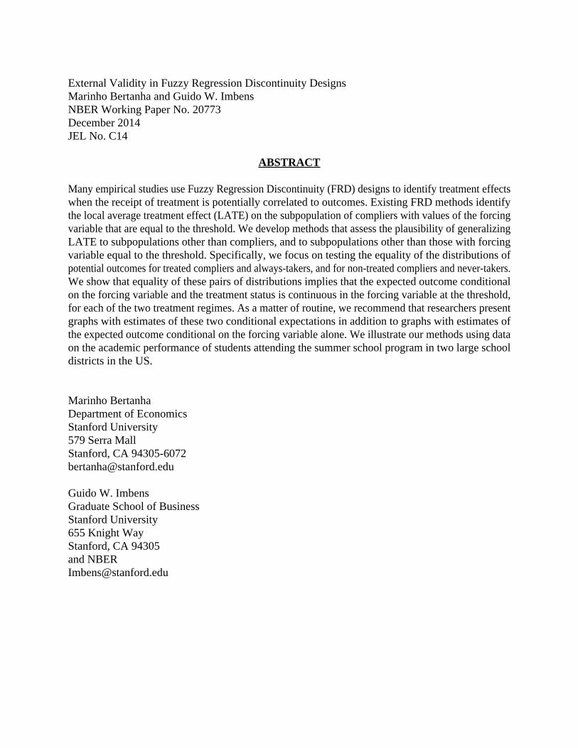
External Validity in Fuzzy Regression Discontinuity DesignsMarinho Bertanha and Guido W. ImbensNBER Working Paper No. 20773December 2014JEL No. C14

ABSTRACT

Many empirical studies use Fuzzy Regression Discontinuity (FRD) designs to identify treatment effectswhen the receipt of treatment is potentially correlated to outcomes. Existing FRD methods identifythe local average treatment effect (LATE) on the subpopulation of compliers with values of the forcingvariable that are equal to the threshold. We develop methods that assess the plausibility of generalizingLATE to subpopulations other than compliers, and to subpopulations other than those with forcingvariable equal to the threshold. Specifically, we focus on testing the equality of the distributions ofpotential outcomes for treated compliers and always-takers, and for non-treated compliers and never-takers.We show that equality of these pairs of distributions implies that the expected outcome conditionalon the forcing variable and the treatment status is continuous in the forcing variable at the threshold,for each of the two treatment regimes. As a matter of routine, we recommend that researchers presentgraphs with estimates of these two conditional expectations in addition to graphs with estimates ofthe expected outcome conditional on the forcing variable alone. We illustrate our methods using dataon the academic performance of students attending the summer school program in two large schooldistricts in the US.

Marinho BertanhaDepartment of EconomicsStanford University579 Serra MallStanford, CA [email protected]

Guido W. ImbensGraduate School of BusinessStanford University655 Knight WayStanford, CA 94305and [email protected]

1 Introduction

In empirical studies in economics and other social sciences researchers are often concerned

about the possible endogeneity of key variables. Recently, many studies have used re-

gression discontinuity designs, originating in the psychology literature (Thistlewaite and

Campbell, 1960) to address these concerns. See Van Der Klaauw (2008), Imbens and

Lemieux (2008), and Lee and Lemieux (2010) for recent surveys, and Cook (2008) for

a historical perspective. In the current paper we study comparisons of regression dis-

continuity estimators and estimators based on unconfoundedness or exogeneity-type as-

sumptions. In the closely related setting of linear instrumental variables models with

constant coefficients, such comparisons are often based on Hausman tests (Hausman,

1978). In the local average treatment (LATE) setting with heterogenous treatment ef-

fects (Imbens and Angrist (1994), Angrist, Imbens and Rubin (1996)), Angrist (2004)

discusses the interpretation of the Hausman test and suggests a more attractive test for

homogeneity of treatment effects in that context. In the current paper, we discuss the

extension of the Hausman and Angrist tests to the fuzzy regression discontinuity (FRD)

settings. Using the FRD set up developed by Hahn, Todd and Van Der Klaauw (2001)

and allowing for heterogeneous treatment effects, we propose a more attractive and novel

test for homogeneity of treatment effects.

In a Hausman test, the parameter estimated by least squares is compared to the

parameter estimated by instrumental variables. In the regression discontinuity context,

the first parameter identifies the average treatment effect at the threshold under exo-

geneity or unconfoundedness assumptions, whereas the second parameter identifies the

average treatment effect at the threshold for the subpopulation of compliers under the

FRD identification assumptions.

Our main point is that, instead of testing the single equality of the Hausman ap-

proach, researchers should test jointly a pair of restrictions on the potential outcomes of

compliers, always-takers, and never-takers using the Imbens-Angrist terminology in the

FRD design. The pair of restrictions are: (i) the equality between the average outcome

of treated always-takers and compliers at the threshold; (ii) the equality between the

average outcome for non-treated never-takers and compliers at the threshold. If both

equalities hold, we argue that is more plausible that one can extrapolate the average

[1]

effect for compliers to other subpopulations; that is, it is more likely that the estimates

have external validity. Moreover, external validity also allows for identification of treat-

ment effects on subpopulations with values for the forcing variable that are different than

the threshold.

We show that this pair of restrictions is equivalent to continuity of the conditional ex-

pectation of the outcome as a function of the forcing variable at the threshold, separately

for each of the two treatment regimes. Currently researchers applying fuzzy regression

discontinuity designs typically present graphs containing estimates of the conditional

expectation of the outcome given the forcing variable without conditioning on the treat-

ment to illustrate the identification strategy. We recommend that, in addition to those

graphs, researchers present graphs containing estimates of the conditional expectations

of the outcome given the forcing variable separately by treatment status. A discontinuity

at the threshold in these conditional expectations provides evidence against exogeneity

or unconfoundedness assumptions, and, thereby, evidence against external validity of the

estimates.

In the recent causal literature there have been alternative proposals for assessing

and improving the external validity of regression discontinuity and instrumental vari-

ables estimates. In an interesting approach, Dong and Lewbel (2014) point out that at

the threshold one cannot only estimate the magnitude of the discontinuity, but also the

change in the first (or even higher order) derivatives of the regression function. Under

smoothness of the two conditional mean functions, knowledge of the higher order deriva-

tives would allow the researcher to extrapolate at least locally away from the threshold.

The Dong and Lewbel methods apply both in the sharp and in the fuzzy regression

discontinuity design. Angrist and Rokkanen (2012) exploit the presence of additional ex-

ogenous covariates, and assess whether conditional on these covariates the influence of the

forcing variable vanishes. This allows for extrapolation away from the threshold. Their

methods also apply both in the case of sharp and fuzzy regression discontinuity designs.

Angrist and Fernandez-Val (2010), in a conventional instrumental variables setting that

can be generalized to the fuzzy regression discontinuity setting, consider extrapolating

local average treatment effects by exploiting the presence of other exogenous covariates.

Their key assumption, which they label conditional effect ignorability, is that conditional

on these additional covariates the average effect for compliers is identical to the aver-

[2]

age effect for all compliance types. These three approaches are all complementary to

ours. In contrast to these extrapolation methods, our approach requires the regression

discontinuity design to be fuzzy but it does not require additional covariates.

The remainder of this paper is organized as follows. In Section 2, we introduce

the notation for the FRD setting, define parameters of interest, and state regularity

and identification conditions. Section 3 discusses methods to assess the plausibility of

exogeneity and external validity. Section 4 illustrates our proposed methods using two

data sets previously used to estimate the effect of summer school programs on academic

performance; the first data set was originally analyzed by Jacob and Lefgren (2004), and

the second data set was previously studied by Matsudaira (2008). An appendix presents

proofs for the results in this paper.

2 Set Up

Here we set up the framework for analyzing fuzzy regression discontinuity designs. We

largely follow the widely used Rubin Causal Model set up, extended to the fuzzy re-

gression discontinuity design by Hahn, Todd, and Van Der Klaauw (2001), HTV from

hereon. Recent theoretical contributions include Porter (2003), McCrary (2008), Imbens

and Kalyanaraman (2012), Calonico, Cattaneo and Titiunik (2014abc), Dong (2014),

Dong and Lewbel (2014), Bertanha (2014), and Gelman and Imbens (2014). Influential

applications include Black (1999), Berk and Rauma (1983), Angrist and Lavy (1999),

Van Der Klaauw (2002), Jacob and Lefgren (2004), Battistin and Rettore (2008), Lee

(2008), Lalive (2008), and Matsudaira (2008).

2.1 Notation

We consider a setting where we have a random sample from a large population, with

the units in the sample indexed by i = 1, . . . , N . Let W obsi be the binary treatment of

interest, which may be endogenous. We are interested in the causal effect of the treatment

on an outcome Yi. Let Yi(0) and Yi(1) denote the potential outcomes. The realized and

observed outcome is

Y obsi =

{Yi(0) if W obs

i = 0,Yi(1) if W obs

i = 1.

[3]

In addition we observe for each unit a covariate, which we refer to as the forcing variable,

denoted by Xi. The support of the distribution of the forcing variable Xi is denoted

by X. The forcing variable is a fixed characteristic of the individual that is not affected

by the treatment. At a particular value for this forcing variable, the threshold, denoted

by T ?, the incentives to participate in the treatment change. We view the value of this

threshold as a quantity that can potentially be manipulated. We assume that changing

the value of the threshold does not change the values of the potential outcomes.

Our set up for the determination of the treatment received is slightly different from

that in HTV, and more line with Dong (2014) and Dong and Lewbel (2014) in that we

explictly allow for different values of the threshold. Let Wi(t) be the potential outcome

denoting whether individual i would participate in the treatment if the threshold was set

equal to t. We assume there are three types of individuals, with the type for individual

i denoted by Gi. First, never-takers, with Gi = n, for whom Wi(t) = 0 for all t. Second,

always-takers, with Gi = a, for whom Wi(t) = 1 for all t, and compliers, with Gi = c,

who participate if the threshold that requires participation is set to the value of their

forcing variable or higher, so that Wi(t) = 1Xi≤t. We observe W obsi = Wi(T

?), at the

actual threshold T ?.

To make this concept more accessible, consider the application we are using in this

paper. In the summer school example the forcing variable Xi is a test-score prior to the

summer program. The school district sets a threshold t, with students scoring below

or at the threshold, that is, students with Xi ≤ t, required to participate in the sum-

mer program. The function Wi(t) describes whether student i would participate in the

program if the district had set the threshold for participation at t. Given the score Xi

for student i, in many cases students would participate if they score less than or equal

to the threshold set by the district, that is, if Xi ≤ t, but not otherwise, so that for

those students the participation decision is Wi(t) = 1Xi≤t. There are some students who

would participate in the summer program even if their score is above the threshold, the

always-takers with Wi(t) = 1, and some students who would not participate even if their

score is below the threshold, the never-takers, with Wi(t) = 0.

[4]

2.2 Causal Estimands

Here we define the main causal estimands.

First, the average causal effect of the treatment for individuals for whom the value of

the forcing variable is equal x:

τ ate(x) = E [Yi(1)− Yi(0)|Xi = x] .

Of particular interest is the average effect for individuals with Xi = T ?:

τ ate(T ?) = E [Yi(1)− Yi(0)|Xi = T ?] .

In addition, define the local average treatment effect,

τ late = E [Yi(1)− Yi(0)|Gi = c, Xi = T ?] .

Define also the overall average effect

τ ate = E [Yi(1)− Yi(0)] = E[τ ate(Xi)

].

2.3 Fuzzy Regression Discontinuity and Exogenous Estimands

Next, we consider what is being estimated by methods that rely on FRD assumptions or

on exogeneity/unconfoundedness type assumptions. First, define

τ frd =limh↓0

{E[Y obs

i |T ? < Xi < T ? + h]− E[Y obsi |T ? − h < Xi < T ?]

}limh↓0

{E[W obs

i |T ? < Xi < T ? + h]− E[W obsi |T ? − h < Xi < T ?]

} .Second, we consider a comparison between treated and control units for the subpopulation

with covariate value close to the threshold:

τ exo = limh↓0

{E[Y obs

i |W obs = 1, T ? − h < Xi < T ? + h]

−E[Y obsi |W obs = 0, T ? − h < Xi < T ? + h]

}.

2.4 Assumptions

We make the following assumptions, which are standard assumptions in the regression

discontinuity literature. See HTV, Lewbel and Dong (2014), Porter (2003), Calonico,

Cattaneo and Titiunik (2014).

[5]

Assumption 1. The sample is a random sample from a large population.

Assumption 2. The probability pr(Yi(0) ≤ y0, Yi(1) ≤ y1, Gi = g|Xi = x) is continuous

in x for all y0, y1 ∈ {−∞,∞} and g ∈ {n, a, c}, and the conditional mean of Yi(w) given

Xi = x is finite for all x and w.

Assumption 3. The distribution of Xi is continuous with density fX(x). The pr(W obsi =

1|Xi = x) is strictly between zero and one for all values of x in the support of Xi.

Assumption 4. The actual threshold is T ?, with the density fX(T ?) positive.

The following result is due to HTV (2001), and it is stated without proof.

Lemma 1. Suppose Assumptions 1-4 hold. Then:

τ frd = τ late.

3 Testing for Exogeneity and External Validity in

Fuzzy Regression Discontinuity Settings

In this section we discuss the main restrictions we wish to assess.

3.1 The Hausman Test in Fuzzy Regression Discontinuity De-signs

To set the stage, let us first consider the standard (that is, non-regression discontinuity)

instrumental variables setting, with a single binary endogenous regressor and a single

binary instrument. In a constant coefficient model we have

Y obsi = α + τ ·W obs

i + εi,

with a binary instrument Zi. The Hausman test compares the ordinary least squares

estimator for τ with the instrumental variables estimator using Zi as an instrument for

W obsi . In large samples the test compares the two quantities,

plim(τ̂ ols) = E[Y obsi |W obs

i = 1]− E[Y obsi |W obs

i = 0],

[6]

with

plim(τ̂ iv) =E[Y obs

i |Zi = 1]− E[Y obsi |Zi = 0]

E[W obsi |Zi = 1]− E[W obs

i |Zi = 0].

The first result explores the interpretation of the restriction plim(τ̂ ols) = plim(τ̂ iv)

settings with heterogenous treatments, under monotonicity, exogeneity of the instrument,

and the exclusion restriction. These are the instrumental variables assumptions used in

Imbens and Angrist (1994) and Angrist, Imbens and Rubin (1996). Let Gi ∈ {n, c, a}denote the compliance type for unit i, let πn = pr(Gi = n), πc = pr(Gi = n), and

πa = pr(Gi = n) denote their population shares, and let pz = Pr(Zi = 1) denote the

population probability that the instrument takes on the value one.

Lemma 2. Suppose that Zi is independent of (Yi(0), Yi(1), Gi), and that there are no

defiers. Then the Hausman null hypothesis

HH,iv0 : plim(τ̂ ols) = plim(τ̂ iv),

is equivalent to the null hypothesis

HH,iv′0 :

πaπa + πc · pz

·(E[Yi(1)|Gi = a]− E[Yi(1)|Gi = c]

)(3.1)

=πn

πn + πc · (1− pz)·(E[Yi(0)|Gi = n]− E[Yi(0)|Gi = c]

).

All proofs are in the Appendix.

In the fuzzy regression design setting, the natural analogue of the Hausman test is

the null hypothesis that the fuzzy regression discontinuity estimand is identical to the

local comparison of treated and control units:

HH,frd0 : τ exo = τ frd. (3.2)

The following lemma shows the equivalence between the equality τ exo = τ frd and a

equality of weighted averages of potential outcomes of compliers, always-takers and never-

takers. Now let πn(x) = pr(Gi = n|Xi = x), πa(x) = pr(Gi = a|Xi = x), and πc(x) =

pr(Gi = c|Xi = x) be the type probabilities conditional on the value of the forcing

variable, and let πn = πn(T ∗), πa = πa(T∗), and πc = πc(T

∗) be shorthand for the type

probabilities at the threshold.

[7]

Lemma 3. Suppose that Assumptions 1-4 hold. Then the null hypothesis

HH,frd0 : τ exo = τ frd,

is equivalent to the null hypothesis

HH,frd′0 :

πaπa + πc/2

·(E[Yi(1)|Gi = a, Xi = T ?]− E[Yi(1)|Gi = c, Xi = T ?]

)=

πnπn + πc/2

·(E[Yi(0)|Gi = n, Xi = T ?]− E[Yi(0)|Gi = c, Xi = T ?]

).

The slight change in the weights comes from the fact that by assumption the prob-

ability of being to the left or to the right of the threshold, conditional on being very

close to the threshold, is equal to 1/2, because of the continuity of the distribution of the

forcing variable.

Comment 1: The first point of the paper is that in general the Hausman hypotheses

HH,iv′0 and HH,frd′

0 are difficult to interpret outside the setting with constant treatment

effects that they were originally developed for. These null hypotheses allow for differ-

ences in average outcomes between always-takers and compliers with the treatment, and

between never-takers and compliers without the treatment, as long as the particular

weighted average of those differences cancel out. The weights depend on the shares of

the compliance types. �

3.2 The Angrist (2004) Restrictions

Angrist (2004) suggests testing for selection bias in the conventional instrumental vari-

ables setting by testing the null hypothesis

HA,iv0 :

E[Y obsi |Zi = 1]− E[Y obs

i |Zi = 0]

E[W obsi |Zi = 1]− E[W obs

i |Zi = 0]

= E[Y obsi |W obs

i = 1, Zi = 0]− E[Y obsi |W obs

i = 0, Zi = 1].

This is equivalent to the null hypothesis

HA,iv′0 : E[Yi(1)− Yi(0)|Gi = c] = E[Yi(1)|Gi = a]− E[Yi(0)|Gi = n],

or, to stress the difference with the Hausman test,

HA,iv′′0 : E[Yi(1)|Gi = a]− E[Yi(1)|Gi = c] = E[Yi(0)|Gi = n]− E[Yi(0)|Gi = c].

[8]

Compared to the Hausman null hypothesis HH,iv′, in the Angrist null hypothesis HA,iv′′

the weights have been dropped, and we simply compare the average effect for compliers

to the difference in average outcomes for always-takers and never-takers, which appears

to be a more natural comparison.

In the fuzzy regression discontinuity setting the natural analogue of Angrist’s null

hypothesis is

HH,frd0 : τ frd = lim

h↓0E[Y obs

i |W obsi = 1, Xi < T ? + h]−E[Y obs

i |W obsi = 0, T ?− h < Xi].

Lemma 4. Suppose that Assumptions 1-4 hold. Then the null hypothesis

HA,frd0 : τ frd = lim

h↓0E[Y obs

i |W obsi = 1, Xi < T ? + h]−E[Y obs

i |W obsi = 0, T ?− h < Xi],

is equivalent to the null hypotheses

HA,frd′0 : E[Yi(1)|Gi = c, Xi = T ?]− E[Yi(0)|Gi = c, Xi = T ?]

= E[Yi(1)|Gi = a, Xi = T ?]− E[Yi(0)|Gi = n, Xi = T ?],

and

HA,frd′′0 : E[Yi(1)|Gi = a, Xi = T ?]− E[Yi(1)|Gi = c, Xi = T ?]

= E[Yi(0)|Gi = n, Xi = T ?]− E[Yi(0)|Gi = c, Xi = T ?].

Angrist (2004) motivates his proposed test by arguments concerning the statistical

power. We view his test also as more attractive than the Hausman test because it has a

more intuitive interpretation.

3.3 External Validity

Under the assumptions we laid out, regression discontinuity estimates are valid locally,

where the qualifier “locally” limits their generalizability in two aspects. These estimates

are valid only for units with the value of the forcing variable Xi close to the threshold

T ?, and they are valid only for compliers. Often we are interested in causal effects

also for non-compliers, and for units with values for the forcing variable away from

the threshold. In this section, we explore the assumptions that validate extrapolation

[9]

(external validity) of treatment effects to individuals with different values of the forcing

variable and individuals of different compliance types.

We consider the following assumption.

Assumption 5. (External Validity)

The study is externally valid if,

Gi ⊥⊥(Yi(0), Yi(1)

) ∣∣∣ Xi. (3.3)

This assumption is related to what Angrist (2004) calls the “no-selection bias” condi-

tion in the conventional instrumental variables setting, and what Dong and Lewbel call

the “local invariance assumption”. Angrist shows that, in the case of binary instrument

and binary treatment, the no-selection assumption leads to four restrictions with two

free parameters, or to a pair of testable restrictions. Here we explore and extend these

findings to the regression discontinuity setting. First, this assumption implies that the

average treatment effect is identified:

Lemma 5. Suppose Assumptions 1-5 hold. Then τ ate is identified.

In the FRD case, we observe treated and non-treated individuals with values for the

forcing variable that are different than the threshold. In general, comparing treated and

non-treated outcomes away from the threshold does not identify treatment effects because

treated and non-treated individuals belong to different compliance subpopulations (i.e.

compliers, always-takers, never-takers). Under external validity, the average potential

outcome does not vary across compliance subpopulations, and the comparison of treated

and non-treated outcomes away from the threshold does identify treatment effects.

Let us now explore the testable restrictions implied by the external validity assump-

tion. External validity implies the following conditional independence restriction:

Gi ⊥⊥ Yi(1)∣∣∣ Xi = T ?. (3.4)

This in turn implies

Gi ⊥⊥ Yi(1)∣∣∣ Gi ∈ {a, c}, Xi = T ?, (3.5)

so that

E[Yi(1)|Gi = c,Xi = T ?] = E[Yi(1)|Gi = a,Xi = T ?], (3.6)

[10]

and, by a similar argument,

E[Yi(0)|Gi = c,Xi = T ?] = E[Yi(0)|Gi = n,Xi = T ?], (3.7)

These two restrictions are still in terms of unobserved variables. However, they imply a

pair of restrictions on observed variables, as summarized in the following lemma.

Lemma 6. Suppose Assumptions 1-5 hold. Then:

limh↓0

E[Y obsi

∣∣W obsi = w, T ? < Xi < T ? + h

]= lim

h↓0E[Y obsi

∣∣W obsi = w, T ? − h < Xi < T ?

], (3.8)

for w = 0, 1.

Comment 2: The two restrictions (3.6) and (3.7) together imply the restriction tested

by the Hausman test, HH,frd′0 , as well as the restriction tested by Angrist’s test, HA,frd′′

0 .

However, the two restrictions are stronger than the restrictions tested by either the

Hausman or the Angrist test on their own. Therefore, testing the pair of restrictions (3.6)

and (3.7) jointly is more attractive. For example, suppose the Angrist null hypothesis

HA,frd′′0 holds, but not the pair of restrictions (3.6) and (3.7). In that case the Angrist

null hypothesis would no longer hold after a transformation of the outcome, say from

Y obsi to ln(Y obs

i ). �

Comment 3: Equation (3.8) is the key equation in the paper. There is a simple graphical

representation of this equality: the expectation of Y obsi conditional on W obs

i = w and Xi is

continuous in the forcing variable at the threshold T ?. This can be assessed by estimating

this conditional expectation E[Y obsi |W obs

i = w,Xi = x] and checking for a discontinuity

at Xi = x, for both w = 0, 1. The implementation is very similar to estimating a

treatment effect in a regression discontinuity design except for the fact that the density

of Xi conditional on Wi = w may be discontinuous at the threshold. �

4 Two Applications

In this section, we illustrate our methods using data from Jacob and Lefgren (2004) and

Matsudaira (2008). These papers estimate the effect of remedial summer school programs

on academic performance of students using fuzzy regression discontinuity methods.

[11]

4.1 The Jacob and Lefgren (2004) Data

In this section, we illustrate the equality of means among different compliance groups in

a FRD setting using data from Jacob and Lefgren (2004). Jacob and Lefgren use admin-

istrative data from the Chicago Public Schools which instituted in 1996 an accountability

policy that tied summer school attendance and promotional decisions to performance on

standardized tests. This policy was followed by other school districts in the country. In

section 4.2, we apply our methods to Matsudaira (2008) data from another urban school

district in the Northeast who adopted a similar policy. The standard rule is to send a

student to summer school if the minimum between his reading and math test-score is

below a certain threshold. The final decision is up to teacher’s discretion which considers

some other indicators which leads to a FRD design.

There are reasons to expect that in this setting those who do not attend summer

school despite scoring below the threshold (never-takers) are different from compliers:

they may have been judged to have scored below expectations and viewed as not in

need of summer school, and thus be better than compliers with similar pre-summer

school scores, or they may be reluctant to participate in summer school and actually be

worse in terms of academic ability than compliers. Similarly, it could be that always-

takers are students viewed as particularly in need of the extra instruction, and thus be

worse in terms of academic ability than compliers with the same scores prior to summer

school, or these could be students that are particularly eager for additional educational

experiences and who would have done better than compliers regardless of their summer

school participation.

Jacob and Lefgren use observations around a test-score cutoff to estimate the impact

of attending summer school on academic performance. They find a positive impact on

achievement for third graders. We use the data for third graders in years 1997-99. The

forcing variable Xi is the minimum between reading and math score before the summer

school minus the threshold (2.75 in this application). The outcome variable Y obsi is

measured by the math score after the summer school.

Following the work by Hahn, Todd and Van Der Klaauw (2001) and Porter (2003), we

fit a local linear regression on each side of the cutoff using the edge kernel k(u) = 1|u|≤1 ·(1−|u|). The optimal bandwidth was computed based on the Imbens and Kalyanaraman

[12]

(2012) optimal bandwidth rule. In Figure 1a we plot the probability of attending summer

school given the value of the forcing variable. Most of the students that are eligible for

summer school based on the minimum test-score do attend summer school, and the

change in the probability of attending summer school is estimated at 0.894 (s.e. 0.006)

(Table 1). Next, in Figure 1b, we plot the conditional mean of the math test-score after

summer school given the minimum test-score prior to summer school. Conditional on

having the minimum test-score close to the threshold, there is a significant increase in the

outcome for those who are required to attend summer school compared to those who are

not required to attend summer school. The causal effect of summer school on subsequent

academic performance for the subpopulation of compliers is around 0.20 (s.e. 0.03).

In the last two figures based on the Jacob-Lefgren data, Figures 1c and 1d, we present

estimates of the expected value of the outcome conditional on both the forcing variable

and treatment status E[Yi|Xi,Wi = w] for w ∈ {0, 1}. We find that there is not a

substantial difference between never-takers and control compliers, with the difference in

average outcomes estimated at 0.07 (s.e. 0.06). On the other hand, there is a substantial

difference in average outcomes between always-takers and treated compliers, at 0.36 (s.e.

0.13). Always-takers perform substantially worse than treated compliers, consistent with

the notion that the always-takers are guided towards the summer program even if they

score slightly above the threshold. In this application, the Hausman and Angrist null

hypotheses are rejected at conventional levels, suggesting heterogeneity of treatment

effects across compliance groups. Our approach finds evidence supporting homogeneity

of treatment effects between compliers and never-takers.

4.2 The Matsudaira (2008) Data

Matsudaira(2008) uses administrative data from a large urban school district in North-

eastern United States to evaluate the impact of attending summer school on students’

academic performance. One of the promotion criteria in this school district requires stu-

dents in third grade or above to score above a given cutoff score on year-end examinations

in both math and reading in order to pass to the next grade. Students who fail to score

above the cutoff are more likely to be required to attend the summer school program.

Besides passing the test-score in reading and math, there are other criteria for promo-

[13]

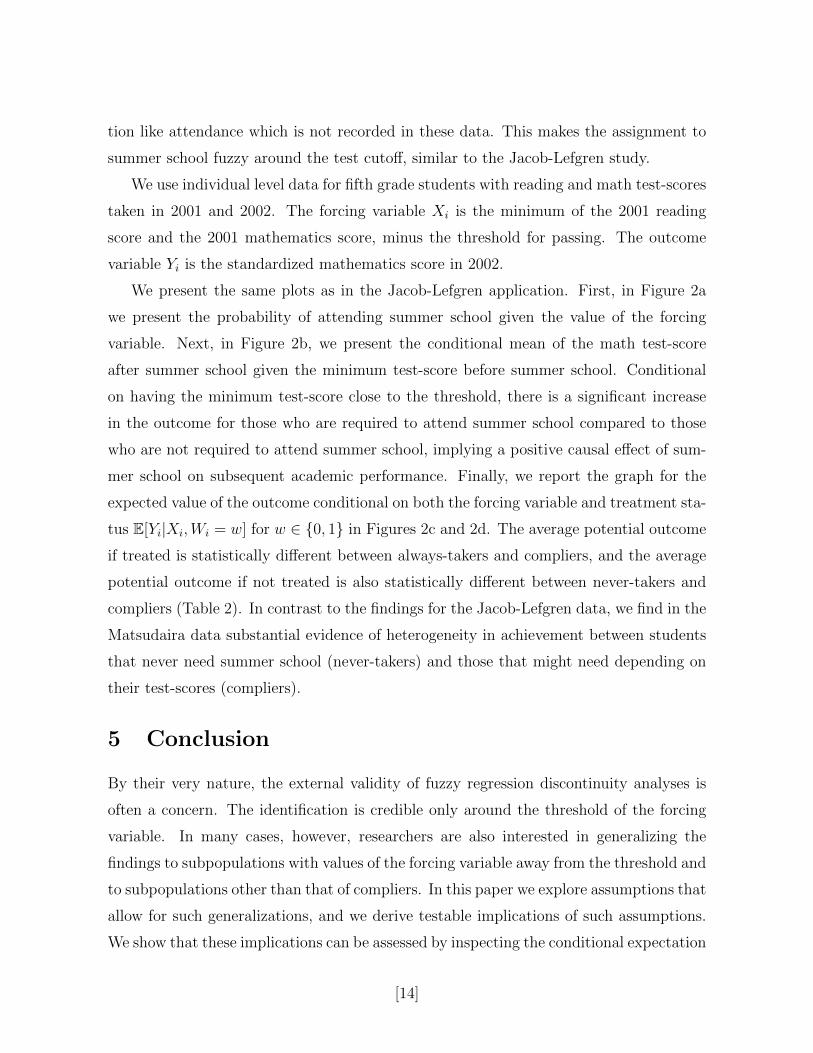
tion like attendance which is not recorded in these data. This makes the assignment to

summer school fuzzy around the test cutoff, similar to the Jacob-Lefgren study.

We use individual level data for fifth grade students with reading and math test-scores

taken in 2001 and 2002. The forcing variable Xi is the minimum of the 2001 reading

score and the 2001 mathematics score, minus the threshold for passing. The outcome

variable Yi is the standardized mathematics score in 2002.

We present the same plots as in the Jacob-Lefgren application. First, in Figure 2a

we present the probability of attending summer school given the value of the forcing

variable. Next, in Figure 2b, we present the conditional mean of the math test-score

after summer school given the minimum test-score before summer school. Conditional

on having the minimum test-score close to the threshold, there is a significant increase

in the outcome for those who are required to attend summer school compared to those

who are not required to attend summer school, implying a positive causal effect of sum-

mer school on subsequent academic performance. Finally, we report the graph for the

expected value of the outcome conditional on both the forcing variable and treatment sta-

tus E[Yi|Xi,Wi = w] for w ∈ {0, 1} in Figures 2c and 2d. The average potential outcome

if treated is statistically different between always-takers and compliers, and the average

potential outcome if not treated is also statistically different between never-takers and

compliers (Table 2). In contrast to the findings for the Jacob-Lefgren data, we find in the

Matsudaira data substantial evidence of heterogeneity in achievement between students

that never need summer school (never-takers) and those that might need depending on

their test-scores (compliers).

5 Conclusion

By their very nature, the external validity of fuzzy regression discontinuity analyses is

often a concern. The identification is credible only around the threshold of the forcing

variable. In many cases, however, researchers are also interested in generalizing the

findings to subpopulations with values of the forcing variable away from the threshold and

to subpopulations other than that of compliers. In this paper we explore assumptions that

allow for such generalizations, and we derive testable implications of such assumptions.

We show that these implications can be assessed by inspecting the conditional expectation

[14]

of the outcome given the forcing variable separately by treatment status. We recommend

that researchers present graphs containing estimates of these conditional expectations and

test for continuity at the threshold.

[15]


+ E[Yi(1)|Gi = c] · πc · pzπa + πc · pz

− E[Yi(1)|Gi = c]

−E[Yi(0)|Gi = n]· πnπn + πc · (1− pz)

+E[Yi(0)|Gi = c]· πc · (1− pz)πn + πc · (1− pz)

−E[Yi(0)|Gi = c]


− E[Yi(1)|Gi = c] · πaπa + πc · pz

−(E[Yi(0)|Gi = n] · πn

πn + πc · (1− pz)− E[Yi(0)|Gi = c] · πn

πn + πc · (1− pz)

)=(E[Yi(1)|Gi = a]− E[Yi(1)|Gi = c]

)· πaπa + πc · pz

−(E[Yi(0)|Gi = n]− E[Yi(0)|Gi = c]

)· πnπn + πc · (1− pz)

.

�

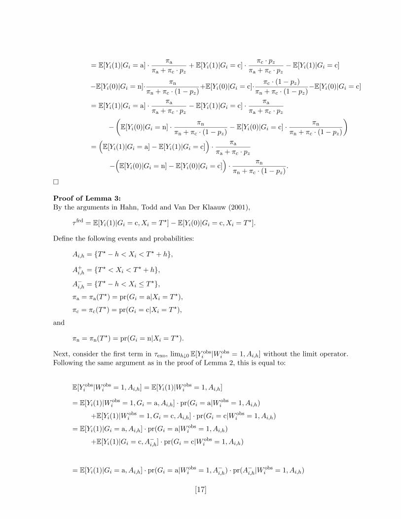
Proof of Lemma 3:By the arguments in Hahn, Todd and Van Der Klaauw (2001),

τ frd = E[Yi(1)|Gi = c, Xi = T ?]− E[Yi(0)|Gi = c, Xi = T ?].

Define the following events and probabilities:

Ai,h = {T ? − h < Xi < T ? + h},

A+i,h = {T ? < Xi < T ? + h},

A−i,h = {T ? − h < Xi ≤ T ?},

πa = πa(T?) = pr(Gi = a|Xi = T ?),

πc = πc(T?) = pr(Gi = c|Xi = T ?),

and

πn = πn(T ?) = pr(Gi = n|Xi = T ?).

Next, consider the first term in τexo, limh↓0 E[Y obsi |W obs

i = 1, Ai,h] without the limit operator.Following the same argument as in the proof of Lemma 2, this is equal to:

E[Y obsi |W obs

i = 1, Ai,h] = E[Yi(1)|W obsi = 1, Ai,h]

= E[Yi(1)|W obsi = 1, Gi = a, Ai,h] · pr(Gi = a|W obs

i = 1, Ai,h)

+E[Yi(1)|W obsi = 1, Gi = c, Ai,h] · pr(Gi = c|W obs

i = 1, Ai,h)

= E[Yi(1)|Gi = a, Ai,h] · pr(Gi = a|W obsi = 1, Ai,h)

+E[Yi(1)|Gi = c, A−i,h] · pr(Gi = c|W obsi = 1, Ai,h)

= E[Yi(1)|Gi = a, Ai,h] · pr(Gi = a|W obsi = 1, A−i,h) · pr(A−i,h|W

obsi = 1, Ai,h)

[17]

+E[Yi(1)|Gi = a, Ai,h] · pr(Gi = a|W obsi = 1, A+

i,h) · pr(A+i,h|W

obsi = 1, Ai,h)

+E[Yi(1)|Gi = c, A−i,h] · pr(Gi = c|W obsi = 1, A−i,h) · pr(A−i,h|W

obsi = 1, Ai,h)

+E[Yi(1)|Gi = c, A−i,h] · pr(Gi = c|W obsi = 1, A+

i,h) · pr(A+i,h|W

obsi = 1, Ai,h)

= E[Yi(1)|Gi = a, Ai,h] · pr(Gi = a|Gi ∈ {a, c}, A−i,h)

·pr(W obs

i = 1|A−i,h)pr(A−i,h)∑s∈{−,+} pr(W obs

i = 1|Asi,h)pr(As

i,h)

+E[Yi(1)|Gi = a, Ai,h] · pr(Gi = a|Gi = a, A+i,h)

·pr(W obs

i = 1|A+i,h)pr(A+

i,h)∑s∈{−,+} pr(W obs

i = 1|Asi,h)pr(As

i,h)

+E[Yi(1)|Gi = c, A−i,h] · pr(Gi = c|Gi ∈ {a, c}, A−i,h)

·pr(W obs

i = 1|A−i,h)pr(A−i,h)∑s∈{−,+} pr(W obs

i = 1|Asi,h)pr(As

i,h)

+E[Yi(1)|Gi = c, A−i,h] · pr(Gi = c|Gi = a, A+i,h)

·pr(W obs

i = 1|A+i,h)pr(A+

i,h)∑s∈{−,+} pr(W obs

i = 1|Asi,h)pr(As

i,h)

= E[Yi(1)|Gi = a, Ai,h] · pr(Gi = a|Gi ∈ {a, c}, A−i,h)

·pr(Gi ∈ {a, c}|A−i,h)

pr(Gi ∈ {a, c}|A−i,h) + pr(Gi = a|A+i,h)pr(A+

i,h)/pr(A−i,h)

+E[Yi(1)|Gi = a, Ai,h] · 1

·pr(Gi = a|A+

i,h)

pr(Gi ∈ {a, c}|A−i,h)pr(A−i,h)/pr(A+i,h) + pr(Gi = a|A+

i,h)

+E[Yi(1)|Gi = c, A−i,h] · pr(Gi = c|Gi ∈ {a, c}, A−i,h)

·pr(Gi ∈ {a, c}|A−i,h)

pr(Gi ∈ {a, c}|A−i,h) + pr(Gi = a|A+i,h)pr(A+

i,h)/pr(A−i,h)

+0

Now, take the limit as h ↓ 0. By assumption, the conditional mean of potential outcomesgiven each compliance type and the forcing variable is a continuous function of the forcingvariable; also, the conditional probability of each compliance type given the forcing variableis a continuous function of the forcing variable; lastly, continuity of the density of the forcingvariable at the threshold implies limh↓0 pr(A−i,h)/pr(A+

i,h) = 1. Therefore,

[18]

limh↓0

E[Y obsi |W obs

i = 1, Ai,h]

= E[Yi(1)|Gi = a, Xi = T ?] · πaπa + πc

· πa + πc2πa + πc

+E[Yi(1)|Gi = a, Xi = T ?] · πa2πa + πc

+E[Yi(1)|Gi = c, Xi = T ?] · πcπa + πc

· πa + πc2πa + πc

= E[Yi(1)|Gi = a, Xi = T ?] · πaπa + πc/2

+ E[Yi(1)|Gi = c, Xi = T ?] · πc/2

πa + πc/2

By a similar argument

limh↓0

E[Y obsi |W obs

i = 0, Ai,h]

= E[Yi(0)|Gi = n, Xi = T ?] · πnπn + πc/2

+ E[Yi(0)|Gi = c, Xi = T ?] · πc/2

πn + πc/2

Finally,

τexo − τ frd

= E[Yi(1)|Gi = a, Xi = T ?] · πaπa + πc/2

+ E[Yi(1)|Gi = c, Xi = T ?] · πc/2

πa + πc/2

−E[Yi(0)|Gi = n, Xi = T ?] · πnπn + πc/2

− E[Yi(0)|Gi = c, Xi = T ?] · πc/2

πn + πc/2

−E[Yi(1)|Gi = c, Xi = T ?] + E[Yi(0)|Gi = c, Xi = T ?]

τexo − τ frd

=πa

πa + πc/2(E[Yi(1)|Gi = a, Xi = T ?])− E[Yi(1)|Gi = c, Xi = T ?]

− πnπn + πc/2

(E[Yi(0)|Gi = n, Xi = T ?]− E[Yi(0)|Gi = c, Xi = T ?])

�

Proof of Lemma 4: The equality of HA,frd′0 and HA,frd′′

0 is immediate. The proof therefore

focuses on the equality of HA,frd′0 and HA,frd

0 . As shown before,

τ frd = E[Yi(1)|Gi = c, Xi = T ?]− E[Yi(0)|Gi = c, Xi = T ?],

[19]

so all that remains to be shown is

limh↓0

E[Y obsi |W obs

i = 1, T ? < Xi < T ? + h]− E[Y obsi |W obs

i = 0, T ? − h < Xi < T ?]


By definition,

limh↓0

E[Y obsi |W obs

i = 1, T ? < Xi < T ? + h]− E[Y obsi |W obs

i = 0, T ? − h < Xi < T ?]

= limh↓0

E[Yi(1)|W obsi = 1, T ? < Xi < T ? + h]− E[Yi(0)|W obs

i = 0, T ? − h < Xi < T ?].

This is equal to

limh↓0

E[Yi(1)|W obsi = 1, Gi = a, T ? < Xi < T ?+h]−E[Yi(0)|W obs

i = 0, Gi = n, T ?−h < Xi < T ?].

= limh↓0

E[Yi(1)|Gi = a, T ? < Xi < T ? + h]− E[Yi(0)|Gi = n, T ? − h < Xi < T ?].


which finishes the proof. �

Proof of Lemma 5: First, notice that

τate = E [E[Yi(1)− Yi(0)|Xi]]

so that it suffices to show that E[Yi(1)− Yi(0)|Xi = x] is identified for every x ∈ X (support ofXi) because the distribution of Xi is identified.

Fix an arbitrary x ∈ X. By external validity (assumption 5), it follows that :

E[Yi(0)|Gi = g,Xi = x] = E[Yi(0)|Xi = x] ∀g ∈ {n, a, c} (A.1)

E[Yi(1)|Gi = g,Xi = x] = E[Yi(1)|Xi = x] ∀g ∈ {n, a, c} (A.2)

Case I: x ≤ T ?

Using the definitions of Gi and W obsi :

Gi ∈ {c, a} ⇐⇒W obsi = 1

∣∣∣ Xi = x (A.3)

Gi = n⇐⇒W obsi = 0

∣∣∣ Xi = x (A.4)

Consider

E[Y obsi |W obs

i = 0, Xi = x]

= E[Yi(0)|W obsi = 0, Xi = x]

[20]

= E[Yi(0)|Gi = n, Xi = x]

= E[Yi(0)|Xi = x]

where we used (A.4) in the second equality, and (A.1) in the third equality.

Next, consider

E[Y obsi |W obs

i = 1, Xi = x]

= E[Yi(1)|W obsi = 1, Xi = x]

= E[Yi(1)|Gi ∈ {c, a}, Xi = x]

= E[Yi(1)|Gi = c, Xi = x] · pr(Gi = c|Gi ∈ {c, a}, Xi = x)

+E[Yi(1)|Gi = a, Xi = x] · pr(Gi = a|Gi ∈ {c, a}, Xi = x)

= E[Yi(1)|Xi = x]

where we used (A.3) in the second equality, and (A.2) in the fourth equality.

Therefore, E[Yi(1)− Yi(0)|Xi = x] is identified in case I.

Case II: x > T ?

Again, by the definitions of Gi and W obsi :

Gi = a⇐⇒W obsi = 1

∣∣∣ Xi = x (A.5)

Gi ∈ {n, c} ⇐⇒W obsi = 0

∣∣∣ Xi = x (A.6)

Consider

E[Y obsi |W obs

i = 0, Xi = x]

= E[Yi(0)|W obsi = 0, Xi = x]

= E[Yi(0)|Gi ∈ {n, c}, Xi = x]

= E[Yi(0)|Gi = n, Xi = x] · pr(Gi = n|Gi ∈ {n, c}, Xi = x)

+E[Yi(0)|Gi = c, Xi = x] · pr(Gi = c|Gi ∈ {n, c}, Xi = x)

= E[Yi(0)|Xi = x]

where we used (A.6) in the second equality, and (A.1) in the fourth equality.

Next, consider

E[Y obsi |W obs

i = 1, Xi = x]

= E[Yi(1)|W obsi = 1, Xi = x]

= E[Yi(1)|Gi = a, Xi = x]

= E[Yi(1)|Xi = x]

where we used (A.5) in the second equality, and (A.2) in the third equality.

Therefore, E[Yi(1)− Yi(0)|Xi = x] is identified in case II.�

Proof of Lemma 6: The claims follow directly from the proof of Lemma 5. �

[21]

References

Angrist, J., (2004), “Treatment Effect Heterogeneity in Theory and Practice,” , The Eco-nomic Journal 114, C52-C83.

Angrist, J., and I. Fernandez-Val, (2010), “ExtrapoLATE-ing: External Validity andOveridentification in the LATE Framework”, NBER Working Paper 16566.

Angrist, J.D., G.W. Imbens, and D.B. Rubin, (1996), Identification of Causal EffectsUsing Instrumental Variables, Journal of the American Statistical Association 91, 444–472.

Angrist, J.D. and A.B. Krueger, (1991), Does Compulsory School Attendance AffectSchooling and Earnings?, Quarterly Journal of Economics 106, 979-1014.

Angrist, J.D., and V. Lavy, (1999), Using Maimonides’ Rule to Estimate the Effect ofClass Size on Scholastic Achievement”, Quarterly Journal of Economics 114, 533-575.

Angrist, J., and M. Rokkanen, (2012), “Wanna Get Away? RD Identification Away fromthe Cutoff”, NBER Working Paper 18662.

Battistin, E. and E. Rettore, (2008), “Ineligibles and Eligible Non-Participants as aDouble Comparison Group in Regression-Discontinuity Designs,” Journal of Economet-rics 142(2), 715-730

Berk, R., and D. Rauma, (1983), “Capitalizing on Nonrandom Assignment to Treat-ments: A Regression-Discontinuity Evaluation of a Crime-Control Program,” Journalof the American Statistical Association, Vol. 78(381): 21-27.

Bertanha, M., (2014), “Regression Discontinuity Design with Many Thresholds,” Unpub-lished Manuscript, Department of Economics, Stanford.

Black, S., (1999), Do Better Schools Matter? Parental Valuation of Elementary Education,Quarterly Journal of Economics 114, 577-599.

Calonico, S., M. Cattaneo, and R. Titiunik, (2014a), “Robust Nonparametric Confi-dence Intervals for Regression-Discontinuity Designs” forthcoming, Econometrica.

Calonico, S., M. Cattaneo, and R. Titiunik, (2014b), “Optimal Data-Driven RegressionDiscontinuity Plots.” Unpublished Working Paper.

Calonico, S., M. Cattaneo, and R. Titiunik, (2014c), “Robust Data-Driven Inferencein the Regression-Discontinuity Design” forthcoming, Stata Journal.

Cattaneo, M., B. Frandsen, and R. Titiunik, (2014), “Randomization Inference inthe Regression Discontinuity Design: An Application to Party Advantages in the U.S.Senate” forthcoming, Journal of Causal Inference.

Cook, T., (2008), “Waiting for Life to Arrive: A History of the Regression-DiscontinuityDesign in Psychology, Statistics and Economics.” Journal of Econometrics, 142(2): 636-54.

[22]

Dong, Y., (2014), “An Alternative Assumption to Identify LATE in Regression DiscontinuityDesigns,” Unpublished Manuscript.

Dong, Y., and A. Lewbel (2014): “Identifying the Effect of Changing the Policy Thresholdin Regression Discontinuity Models” forthcoming, Review of Economics and Statistics.

Gelman, A., and G. Imbens, , (2014), “Why High-Order Polynomials Should Not Be Usedin Regression Discontinuity Designs,” NBER Working Paper 20405.

Hahn, J., P. Todd and W. Van der Klaauw, (2001), Identification and Estimation ofTreatment Effects with a Regression Discontinuity Design, Econometrica 69, 201-209.

Imbens, G., and J. Angrist, (1994), “Identification and Estimation of Local Average Treat-ment Effects”, Econometrica 61, 467-476.

Imbens, G., and K. Kalyanaraman, (2012), “Optimal Bandwidth Choice for the Regres-sion Discontinuity Estimator,” Review of Economic Studies 79(3), 933-959

Imbens, G., and T. Lemieux, (2008), “Regression Discontinuity Designs: A Guide to Prac-tice,” Journal of Econometrics, Vol. 142(2): 615-35.

Jacob, B.A., and L. Lefgren, (2004), Remedial Education and Student Achievement: ARegression-Discontinuity Analysis, Review of Economics and Statistics 68, 226-244.

Lalive, R., (2008), How do Extended Benefits affect Unemployment Duration? A RegressionDiscontinuity Approach, Journal of Econometrics, 142(2), 785-806

Lee, D., (2008), “Randomized Experiments from Non-random Selection in U.S. House Elec-tions,” Journal of Econometrics, 142(2) 675697

Lee, D., and T. Lemieux, (2010), “Regression Discontinuity Designs in Economics,” Journalof Economic Literature, Vol. 48, 281-355.

Ludwig, J., and D. Miller, (2005), Does Head Start Improve Children’s Life Chances?Evidence from a Regression Discontinuity Design, NBER working paper 11702.

Ludwig, J., and D. Miller, (2007), Does Head Start Improve Children’s Life Chances?Evidence from a Regression Discontinuity Design, Quarterly Journal of Economics 122(1),159-208.

Matsudaira, J., (2008), “Mandatory Summer School and Student Achievement”, Journalof Econometrics, 142(2) 829850.

McCrary, J., (2008), “Testing for Manipulation of the Running Variable in the RegressionDiscontinuity Design,” Journal of Econometrics, 142(2) 698714.

Porter, J., (2003), Estimation in the Regression Discontinuity Model,” mimeo, Departmentof Economics, University of Wisconsin, http://www.ssc.wisc.edu/ jporter/reg discont 2003.pdf.

Rubin, D., (1974), Estimating Causal Effects of Treatments in Randomized and Non-randomizedStudies, Journal of Educational Psychology 66, 688-701.

[23]

Thistlewaite, D., and D. Campbell, (1960), Regression-Discontinuity Analysis: An Al-ternative to the Ex-Post Facto Experiment, Journal of Educational Psychology 51, 309-317.

Trochim, W., (1984), Research Design for Program Evaluation; The Regression-DiscontinuityDesign (Sage Publications, Beverly Hills, CA).

Trochim, W., (2001), Regression-Discontinuity Design, in N.J. Smelser and P.B Baltes, eds.,International Encyclopedia of the Social and Behavioral Sciences 19 (Elsevier North-Holland, Amsterdam) 12940-12945.

Van Der Klaauw, W., (2002), Estimating the Effect of Financial Aid Offers on CollegeEnrollment: A Regression-Discontinuity Approach, International Economic Review 43,1249-1287.

Van Der Klaauw, W., (2008) “Regression-Discontinuity Analysis: A Survey of RecentDevelopments in Economics.”Labour, Vol. 22(2): 21945.

[24]

Table 1: Jacob-Lefgren Data

Estimand Estimate s.e. p-valueEstimates

Participation πc 0.894 (0.006 )πa 0.016 (0.002 )πn 0.090 (0.005 )

Cond. Means of E[Yi(1)|Xi = T ∗, Gi = c] 4.394 (0.016 )Potential Outcomes E[Yi(1)|Xi = T ∗, Gi = a] 4.037 (0.124 )

E[Yi(0)|Xi = T ∗, Gi = c] 4.197 (0.017 )E[Yi(0)|Xi = T ∗, Gi = n] 4.267 (0.048 )

LATE E[Yi(1)− Yi(0)|Xi = T ∗, Gi = c] 0.197 (0.025 )

OLS limh↓0 E[Y obsi |W obsi = 1, T ∗ − h < Xi < T ∗ + h] 0.173 (0.021 )

− limh↓0 E[Y obsi |W obsi = 0, T ∗ − h < Xi < T ∗ + h]

Tests

Hausman πa

πa+πc/2· 0.024 (0.011 ) 0.026(

E[Yi(1)|Xi = T ∗, Gi = c]− E[Yi(1)|Xi = T ∗, Gi = a])

− πn

πn+πc/2·(

E[Yi(0)|Xi = T ∗, Gi = c]− E[Yi(0)|Xi = T ∗, Gi = n])

Angrist(E[Yi(1)|Xi = T ∗, Gi = c]− E[Yi(1)|Xi = T ∗, Gi = a]

)0.427 (0.139 ) 0.002

−(E[Yi(0)|Xi = T ∗, Gi = c]− E[Yi(0)|Xi = T ∗, Gi = n]

)Conditional E[Yi(1)|Xi = T ∗, Gi = c]− E[Yi(1)|Xi = T ∗, Gi = a] 0.357 (0.126 ) 0.005

Jumps E[Yi(0)|Xi = T ∗, Gi = c]− E[Yi(0)|Xi = T ∗, Gi = n] -0.070 (0.056 ) 0.213

Joint F-test 9.431 0.009

Notes: Outcome variable Y is the math score (after the summer school), and forcing variable X is theminimum between the reading and math score (before the summer school) minus the cutoff; W is theparticipation indicator. Non-parametric estimates are obtained by local linear regression and optimalbandwidth h = 0.54 by Imbens and Kalyanaraman (2012). The standard errors of all estimates arecomputed using 1000 bootstrap iterations. The F-test is a χ2 statistic computed as a quadratic form ofthe 2×1 vector of the differences between potential outcomes for treated compliers and always-takers andfor non-treated compliers and never-takers inversely weighted by the covariance matrix of such vector.

[25]

Figure 1: Jacob and Lefgren

(a)

−2 −1 0 1 20

0.2

0.4

0.6

0.8

1P(W=1|X), binwidth=0.2

(b)

−2 −1 0 1 22.5

3

3.5

4

4.5

5

5.5

6

6.5

7

7.5E(Y|X), binwidth=0.2

outc

ome

var:

mat

h

(c)

−2 −1 0 1 22.5

3

3.5

4

4.5

5

5.5

6

6.5

7

7.5E(Y|W=0,X), binwidth=0.2

outc

ome

var:

mat

h

(d)

−2 −1 0 1 22.5

3

3.5

4

4.5

5

5.5

6

6.5

7

7.5E(Y|W=1,X), binwidth=0.2

outc

ome

var:

mat

h

Notes: Outcome variable Y is the math score (after the summer school), and forcing variable X is theminimum between the reading and math score (before the summer school) minus the cutoff; W is theparticipation indicator. Step functions are made of local averages within each bin, and plots have thesame number of equal sized bins on each side of the cutoff.

[26]

Table 2: Matsudaira Data

Estimand Estimate s.e. p-valueEstimates

Participation πc 0.400 (0.010 )πa 0.131 (0.005 )πn 0.469 (0.008 )

Cond. Means of E[Yi(1)|Xi = T ∗, Gi = c] -0.213 (0.017 )Potential Outcomes E[Yi(1)|Xi = T ∗, Gi = a] -0.359 (0.023 )

E[Yi(0)|Xi = T ∗, Gi = c] -0.413 (0.022 )E[Yi(0)|Xi = T ∗, Gi = n] -0.325 (0.011 )

LATE E[Yi(1)− Yi(0)|Xi = T ∗, Gi = c] 0.200 (0.027 )

OLS limh↓0 E[Y obsi |W obsi = 1, T ∗ − h < Xi < T ∗ + h] 0.080 (0.012 )

− limh↓0 E[Y obsi |W obsi = 0, T ∗ − h < Xi < T ∗ + h]

Tests

Hausman πa

πa+πc/2· 0.120 (0.025 ) 0.000(

E[Yi(1)|Xi = T ∗, Gi = c]− E[Yi(1)|Xi = T ∗, Gi = a])

− πn

πn+πc/2·(

E[Yi(0)|Xi = T ∗, Gi = c]− E[Yi(0)|Xi = T ∗, Gi = n])

Angrist(E[Yi(1)|Xi = T ∗, Gi = c]− E[Yi(1)|Xi = T ∗, Gi = a]

)0.234 (0.044 ) 0.000

−(E[Yi(0)|Xi = T ∗, Gi = c]− E[Yi(0)|Xi = T ∗, Gi = n]

)Conditional E[Yi(1)|Xi = T ∗, Gi = c]− E[Yi(1)|Xi = T ∗, Gi = a] 0.146 (0.033 ) 0.000

Jumps E[Yi(0)|Xi = T ∗, Gi = c]− E[Yi(0)|Xi = T ∗, Gi = n] -0.088 (0.030 ) 0.003

Joint F-test 28.658 0.000

The forcing variable X is the 2001 minimum score between reading and math minus the cutoff forpassing. The outcome variable Y is the standardized math score in 2002, and W is the participationindicator. Non-parametric estimates are obtained by local linear regression and optimal bandwidthh = 28 by Imbens and Kalyanaraman (2012). The standard errors of all estimates are computed using1000 bootstrap iterations. The F-test is a χ2 statistic computed as a quadratic form of the 2×1 vector ofthe differences between potential outcomes for treated compliers and always-takers and for non-treatedcompliers and never-takers inversely weighted by the covariance matrix of such vector.

[27]

Figure 2: Matsudaira

(a)

−60 −40 −20 0 20 40 600

0.2

0.4

0.6

0.8

1P(W=1|X), binwidth=3.9

(b)

−60 −40 −20 0 20 40 60−2

−1.5

−1

−0.5

0

0.5

1

1.5

2E(Y|X), binwidth=3.9

outc

ome

var:

mat

h

(c)

−60 −40 −20 0 20 40 60−2

−1.5

−1

−0.5

0

0.5

1

1.5

2E(Y|W=0,X), binwidth=3.9

outc

ome

var:

mat

h

(d)

−60 −40 −20 0 20 40 60−2

−1.5

−1

−0.5

0

0.5

1

1.5

2E(Y|W=1,X), binwidth=3.9

outc

ome

var:

mat

h

Notes: The forcing variable X is the 2001 minimum score between reading and math minus the cutofffor passing. The outcome variable Y is the standardized math score in 2002, and W is the participationindicator. Step functions are made of local averages within each bin, and plots have the same numberof equal sized bins on each side of the cutoff.

[28]

External Validity in Fuzzy Regression Discontinuity Designs · External Validity in Fuzzy...

Documents

Transcript of External Validity in Fuzzy Regression Discontinuity Designs · External Validity in Fuzzy...