
Realtime Ray Tracing on current CPU Architectures · Realtime Ray Tracing on current CPU...
210
Realtime Ray Tracing on current CPU Architectures Carsten Benthin Computer Graphics Group Saarland University 66123 Saarbr ¨ ucken, Germany Dissertation zur Erlangung des Grades Doktor der Ingenieurwissenschaften (Dr.-Ing.) der Naturwissenschaftlich-Technischen Fakult¨ at I der Universit¨ at des Saarlandes S A R A V I E N S I S U N I V E R S I T A S
Transcript of Realtime Ray Tracing on current CPU Architectures · Realtime Ray Tracing on current CPU...

Realtime Ray Tracing
on current CPU Architectures
Carsten BenthinComputer Graphics Group
Saarland University66123 Saarbrucken, Germany
Dissertation zur Erlangung des GradesDoktor der Ingenieurwissenschaften (Dr.-Ing.)der Naturwissenschaftlich-Technischen Fakultat Ider Universitat des Saarlandes
SA
RA V I E N
SI
S
UN
I VE R S I T
AS

Betreuender Hochschullehrer / Supervisor:Prof. Dr.-Ing. Philipp SlusallekUniversitat des Saarlandes, Saarbrucken, Germany
Gutachter / Reviewers:Prof. Dr.-Ing. Philipp SlusallekUniversitat des Saarlandes, Saarbrucken, Germany
Prof. Dr. rer. nat. Hans-Peter SeidelMPI Informatik, Saarbrucken, Germany
Research Assistant Professor Steven G. ParkerUniversity of Utah, Salt Lake City, UT, USA
Dekan / Dean:Prof. Dr. rer. nat. Jorg EschmeierUniversitat des Saarlandes, Saarbrucken, Germany
Eingereicht am / Thesis submitted:
30. Januar 2006 / Jan 30st, 2006
Carsten BenthinLehrstuhl fur Computergraphik, Geb. 36.1/E14Im Stadtwald, 66123 [email protected]

iii
Abstract
In computer graphics, ray tracing has become a powerful tool for generatingrealistically looking images. Even though ray tracing offers high flexibility,a logarithmic scalability in scene complexity, and is known to be efficientlyparallelizable, its demand for compute power has in the past lead to itslimitation to high-quality off-line rendering.
This thesis focuses on the question of how realtime ray tracing can be re-alized on current processor architectures. To this end, it provides a detailedanalysis of the weaknesses and strengths of current processor architectures,for the purpose of allowing for highly optimized implementation. The com-bination of processor-specific optimizations with algorithms that exploit thecoherence of ray tracing, makes it possible to achieve realtime performanceon a single CPU.
Besides the optimization of the ray tracing algorithm itself, this thesisfocuses on the efficient building of spatial index structures. By buildingthese structures from scratch for every frame, interactive ray tracing of fullydynamic scenes becomes possible. Moreover, a parallelization framework forray tracing is discussed that efficiently exploits the compute power of a clusterof commodity PCs. Finally, a global illumination algorithm is proposed thatefficiently combines optimized ray tracing and the parallelization framework.The combination makes it possible to compute complete global illuminationat interactive frame rates.

iv
Kurzfassung
In der Computer-Graphik hat sich Ray-Tracing langst als wichtiges Werkzeugzur realistischen Bildsynthese etabliert. Entscheidend dazu beigetragen habendessen Flexibilitat und logarithmische Skalierung in der Szenengroße, sowiedie effiziente Parallelisierbarkeit. Aufgrund der hohen Anforderung an Rechen-kapazitat war die Verwendung bisher auf den qualitativ hochwertigen, abernicht interaktiven Bereich der realistischen Bildsynthese beschrankt.
Diese Dissertation beschaftigt sich mit der Frage, wie die Geschwindigkeitvon Ray-Tracing auf heutigen Prozessorarchitekturen derart gesteigert wer-den kann, dass es die Bildsynthese in Echtzeit ermoglicht. Dazu prasen-tiert die vorliegende Arbeit eine genaue Analyse der Starken und Schwachender heutigen Prozessorarchitekturen, um die benotigten Algorithmen ent-sprechend zu optimieren. Darauf aufbauend werden Algorithmen vorgestellt,die es im besonderen Maße erlauben, Koharenz innerhalb des Ray-TracingVerfahrens effizient auszunutzen. Diese Kombination von koharenz-ausnutzen-den Algorithmen mit einer prozessoroptimierten Implementierung ermoglichtsogar die interaktive Bildsynthese bei Ausnutzung der Rechenkapazitat eineseinzelnen Prozessors.
Daruber hinaus prasentiert die vorliegende Arbeit einen neuen Algorith-mus, der die Zeit fur den Aufbau der fur das Ray-Tracing benotigten raum-lichen Beschleunigungsdatenstrukturen erheblich verkurzt. Der beschleu-nigte Aufbau erlaubt sogar das interaktive Ray-Tracing von vollstandig dy-namischen Szenen. Daneben wird ein Parallelisierungsystem fur Ray-Tracingvorgestellt, welches die Rechenkapazitat eines Netzwerkes von Standardrech-nern effizient kombiniert, um sogar Bildsynthese in Echtzeit zu erreichen.Abschließend wird ein Verfahren zur physikalisch korrekten Beleuchtungssim-ulation beschrieben, welches bereits vorgestellte Techniken wie optimiertesRay-Tracing und effiziente Parallelisierung verbindet. Diese Kombinationermoglicht es letztendlich die physikalisch korrekte Beleuchtung mehrmalspro Sekunde komplett neu zu berechnen.
v
Zusammenfassung
In der Computer-Graphik hat sich Ray-Tracing langst als wichtiges Werkzeugzur realistischen Bildsynthese etabliert. Entscheidend dazu beigetragen habendie Flexibilitat und logarithmische Skalierung in der Szenengroße sowie dieeffiziente Parallelisierbarkeit des Ray-Tracing Verfahrens an sich. Aufgrundder langen Laufzeit und der hohen Anfordung an Rechenkapazitat war dieVerwendung von Ray-Tracing bisher auf den qualitativ hochwertigen, abernicht interaktiven Bereich der realistischen Bildsynthese beschrankt.
Diese Dissertation beschaftigt sich mit der Frage, wie die Geschwindigkeitvon Ray-Tracing derart gesteigert werden kann, dass Ray-Tracing auch furdie interaktive Bildsynthese bzw. die Bildsynthese in Echtzeit geeignet ist.Als ersten Schritt dazu prasentiert die vorliegende Arbeit eine genaue Anal-yse der heutigen Prozessorarchitekturen, die die zugrundeliegende Hardware-Plattform bilden. Dabei werden deren Starken und Schwachen detailliertaufgezeigt und daraus abgeleitet Implementierungs- und Optimierungsricht-linien vorgestellt. Diese Richtlinien erlauben es, ineffizienten Code bei derImplementierung des Ray-Tracing Verfahrens zu vermeiden.
Einer der Hauptschwerpunkte der vorliegenden Disseration liegt auf derEntwicklung von Algorithmen, die es erlauben Koharenz innerhalb des Ray-Tracing Verfahrens effizient auszunutzen. Gerade die Anwendung von Oper-ationen auf koharente Strahlbundel anstatt auf einzelne Strahlen ermoglichteine erhebliche Steigerung der Geschwindigkeit von Ray-Tracing. Dies wirddetailliert an den zwei fundamentalen Algorithmen des Ray-Tracing Ver-fahrens, der Traversierung von Strahlen durch eine raumliche Beschleuni-gungsdatenstruktur und dem Schnittpunkttest zwischen Strahl und geome-trischem Primitive aufgezeigt. Beim Schnittpunkttest wird neben der Unter-stutzung fur Dreiecke ein besonderes Augenmerk auf die effiziente Unter-stutzung von Freiformflachen gelegt. Im Gegensatz zur Beschreibung einerSzene mittels Dreiecken erlaubt die Beschreibung mittels Freiformflacheneine viel kompaktere und genauere Reprasentation. Allerdings gestaltet sichder benotigte Schnittpunkttest ungleich aufwendiger. Diese Arbeit stelltdazu verschiedene Algorithmen vor, die je nach Anwendungsgebiet und Ge-nauigkeitsanforderungen unterschiedlich eingesetzt werden konnen. Die Kom-bination koharenz-ausnutzender Algorithmen zur Traversierung und Schnitt-punktberechnung mit einer effizienten und prozessornahen Implementierungermoglicht sogar die interaktive Bildsynthese bei Ausnutzung der Rechen-kapazitat eines einzelnen Prozessors.
Neben der Optimierung des Ray-Tracing Verfahrens an sich, stellt dieseDissertation ein Algorithmus vor, um die fur Ray-Tracing benotigten raum-lichen Beschleunigungsdatenstrukturen effizient aufzubauen. Dabei wird auf

vi
dieselben Optimierungsstrategien zuruckgegriffen, die bereits bei der Be-schleunigung des Ray-Tracing Verfahrens zum Tragen kommen. Der op-timierte Aufbaualgorithmus erlaubt sogar das interaktive Ray-Tracing vonvollstandig dynamischen Szenen, indem die Beschleunigungsdatenstrukturenmehrmals pro Sekunde komplett neu aufgebaut werden.
Weiterhin wird ein System zur Parallelisierung des Ray-Tracing Ver-fahrens prasentiert, das die Rechenkapazitat eines Netzwerkes von Standard-rechnern effizient kombiniert. Dabei wird das System mit dem Ziel entwickelt,die Nachteile einer solchen verteilten Architektur, wie beispielsweise getren-nte Hauptspeicher und langsame Verbindungsbandbreiten, effizient zu kom-pensieren. So gelingt es, die Geschwindigkeit von Ray-Tracing linear mit derAnzahl der verbundenen Rechner zu steigern, wodurch Ray-Tracing sogar inEchtzeit ermoglicht wird.
Im letzten Teil der Dissertation wird ein Verfahren zur physikalisch kor-rekten Beleuchtungssimulation vorgestellt, welches die bereits vorgestellteTechniken, hoch optimierter Ray-Tracing Kern und Rahmenwerk zur Paral-lelisierung, effektiv verbindet. Die Kombination dieser Techniken mit einemauf Koharenzausnutzung ausgelegtem Algorithmus zur Beleuchtungssimula-tion ermoglicht es letztendlich, die physikalisch korrekte Beleuchtung mehr-mals pro Sekunde komplett neu zu berechnen.

vii
Acknowledgements
First of all, I would like to thank Prof. Dr. Philipp Slusallek for supervis-ing this thesis. The open and encouraging atmosphere in his group and inparticular his continuous support were invaluable for the success of my thesis.
Second, I have to thank Dr. Ingo Wald, who taught me basically ev-erything I know about ray tracing. He has been an invaluable help in manyprojects related to this thesis. Without his encouraging support and a count-less number of discussions through the years I would not have been able tocomplete my PhD thesis.
I would also like to thank my reviewers, Hans-Peter Seidel and StevenParker, for kindly accepting the responsibility of reviewing my thesis.
Similarly, I have to thank (in random order) Andreas Dietrich, HeikoFriedrich, Johannes Gunther, Jorg Schmittler, and Georg Demme and hisadministration group for many fruitful discussions, ideas and help in manyprojects. Special thanks goes to Michael Scherbaum for reducing my work-load during writing this thesis. Furthermore, I would like to thank the currentand former members and students of the computer graphics group.
I would also like to thank James T. Hurley for giving me the opportunityto do an internship at Intel Corp. Many thanks are due to Gordon Stolland Alexander Reshetov for many helpful discussions, for introducing me tomany new ideas, and for simply making the stay a great experience.
Special thanks goes to my sister Nicole Benthin, who helped me writingthis thesis in ’readable’ English.
Finally, and most importantly, I would like to thank my familiy, and inparticular my wife Andrea for their great patience, their encouraging supportand for bearing so many stressful times. Without their help this thesis wouldnever have been possible.

viii
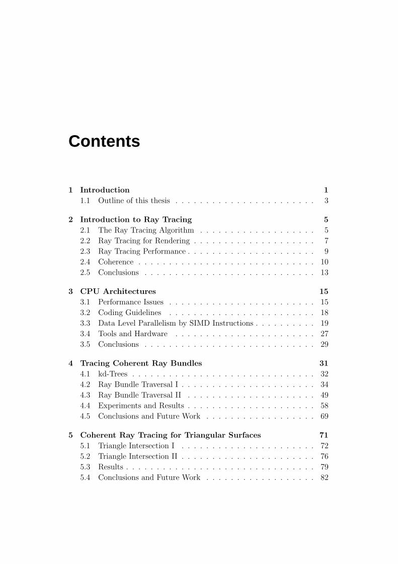
Contents
1 Introduction 1
1.1 Outline of this thesis . . . . . . . . . . . . . . . . . . . . . . . 3
2 Introduction to Ray Tracing 5
2.1 The Ray Tracing Algorithm . . . . . . . . . . . . . . . . . . . 5
2.2 Ray Tracing for Rendering . . . . . . . . . . . . . . . . . . . . 7
2.3 Ray Tracing Performance . . . . . . . . . . . . . . . . . . . . . 9
2.4 Coherence . . . . . . . . . . . . . . . . . . . . . . . . . . . . . 10
2.5 Conclusions . . . . . . . . . . . . . . . . . . . . . . . . . . . . 13
3 CPU Architectures 15
3.1 Performance Issues . . . . . . . . . . . . . . . . . . . . . . . . 15
3.2 Coding Guidelines . . . . . . . . . . . . . . . . . . . . . . . . 18
3.3 Data Level Parallelism by SIMD Instructions . . . . . . . . . . 19
3.4 Tools and Hardware . . . . . . . . . . . . . . . . . . . . . . . 27
3.5 Conclusions . . . . . . . . . . . . . . . . . . . . . . . . . . . . 29
4 Tracing Coherent Ray Bundles 31
4.1 kd-Trees . . . . . . . . . . . . . . . . . . . . . . . . . . . . . . 32
4.2 Ray Bundle Traversal I . . . . . . . . . . . . . . . . . . . . . . 34
4.3 Ray Bundle Traversal II . . . . . . . . . . . . . . . . . . . . . 49
4.4 Experiments and Results . . . . . . . . . . . . . . . . . . . . . 58
4.5 Conclusions and Future Work . . . . . . . . . . . . . . . . . . 69
5 Coherent Ray Tracing for Triangular Surfaces 71
5.1 Triangle Intersection I . . . . . . . . . . . . . . . . . . . . . . 72
5.2 Triangle Intersection II . . . . . . . . . . . . . . . . . . . . . . 76
5.3 Results . . . . . . . . . . . . . . . . . . . . . . . . . . . . . . . 79
5.4 Conclusions and Future Work . . . . . . . . . . . . . . . . . . 82

x CONTENTS
6 Coherent Ray Tracing for Freeform Surfaces 83
6.1 Bezier Fundamentals . . . . . . . . . . . . . . . . . . . . . . . 856.2 The Ray-Patch Intersection Problem . . . . . . . . . . . . . . 906.3 Uniform Refinement . . . . . . . . . . . . . . . . . . . . . . . 916.4 Newton Iteration . . . . . . . . . . . . . . . . . . . . . . . . . 976.5 Newton Iteration and Krawczyk Operator . . . . . . . . . . . 1046.6 Bezier Clipping . . . . . . . . . . . . . . . . . . . . . . . . . . 1136.7 Summary of Intersection Algorithms . . . . . . . . . . . . . . 1236.8 Spatial Index Structures for Patches . . . . . . . . . . . . . . . 1256.9 Trimming Curves . . . . . . . . . . . . . . . . . . . . . . . . . 1256.10 Results . . . . . . . . . . . . . . . . . . . . . . . . . . . . . . . 1286.11 Application . . . . . . . . . . . . . . . . . . . . . . . . . . . . 1356.12 Conclusions and Future Work . . . . . . . . . . . . . . . . . . 138
7 Dynamic Scenes 139
7.1 Rapid Construction of kd-Trees . . . . . . . . . . . . . . . . . 1407.2 Conclusions and Future Work . . . . . . . . . . . . . . . . . . 148
8 Distributed Coherent Ray Tracing on Clusters 149
8.1 Introduction . . . . . . . . . . . . . . . . . . . . . . . . . . . . 1498.2 Distribution Strategies . . . . . . . . . . . . . . . . . . . . . . 1508.3 The OpenRT Distribution Framework . . . . . . . . . . . . . . 1528.4 Communication and Dataflow . . . . . . . . . . . . . . . . . . 1578.5 Results . . . . . . . . . . . . . . . . . . . . . . . . . . . . . . . 1598.6 Conclusions and Future Work . . . . . . . . . . . . . . . . . . 159
9 Applications 163
9.1 Instant Global Illumination . . . . . . . . . . . . . . . . . . . 1639.2 Exploiting Coherence . . . . . . . . . . . . . . . . . . . . . . . 1659.3 Streaming Computations . . . . . . . . . . . . . . . . . . . . . 1679.4 Efficient Anti-Aliasing . . . . . . . . . . . . . . . . . . . . . . 1699.5 Distributed Rendering . . . . . . . . . . . . . . . . . . . . . . 1709.6 Results . . . . . . . . . . . . . . . . . . . . . . . . . . . . . . . 1719.7 Conclusions and Future Work . . . . . . . . . . . . . . . . . . 173
10 Final Summary, Conclusions, and Future Work 175
A List of Related Papers 179
Bibliography 183

List of Figures
2.1 Recursive ray tracing . . . . . . . . . . . . . . . . . . . . . . . 82.2 Ray coherence . . . . . . . . . . . . . . . . . . . . . . . . . . . 11
3.1 SOA data layout . . . . . . . . . . . . . . . . . . . . . . . . . 203.2 Intel’s streaming SIMD extension (SSE) . . . . . . . . . . . . 213.3 AOS vs. SOA . . . . . . . . . . . . . . . . . . . . . . . . . . . 223.4 Parallel dot products using SSE instructions . . . . . . . . . . 223.5 Parallel dot products using SSE intrinsics . . . . . . . . . . . . 243.6 SSE utility functions . . . . . . . . . . . . . . . . . . . . . . . 263.7 SSE inverse computation using Newton-Raphson approximation 263.8 SSE horizontal operations . . . . . . . . . . . . . . . . . . . . 273.9 Data structure for single rays and ray bundles . . . . . . . . . 283.10 Data structure for an axis-aligned bounding box . . . . . . . . 29
4.1 Layout of a kd-tree node . . . . . . . . . . . . . . . . . . . . . 344.2 Traversal order for single rays . . . . . . . . . . . . . . . . . . 354.3 Traversal algorithm for single rays . . . . . . . . . . . . . . . . 364.4 Traversal algorithm for ray bundles . . . . . . . . . . . . . . . 374.5 Ray bundle initialization . . . . . . . . . . . . . . . . . . . . . 394.6 Traversal order look-up table . . . . . . . . . . . . . . . . . . . 404.7 Traversal implementation for a single four-ray bundle . . . . . 424.8 Traversal implementation without branches . . . . . . . . . . . 454.9 Traversal implementation for four-ray bundles . . . . . . . . . 464.10 Alternative traversal implementation for four-ray bundles . . . 484.11 Inverse frustum culling algorithm . . . . . . . . . . . . . . . . 504.12 Offset look-up table for extremal traversal . . . . . . . . . . . 524.13 Extremal traversal implementation by inverse frustum culling . 534.14 Alternative extremal traversal algorithm . . . . . . . . . . . . 544.15 Alternative ray-segment traversal implementation for extremal
traversal . . . . . . . . . . . . . . . . . . . . . . . . . . . . . . 554.16 Finding kd-tree entry points . . . . . . . . . . . . . . . . . . . 56
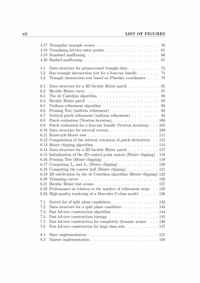
xii LIST OF FIGURES
4.17 Triangular example scenes . . . . . . . . . . . . . . . . . . . . 584.18 Visualizing kd-tree entry points . . . . . . . . . . . . . . . . . 614.19 Standard mailboxing . . . . . . . . . . . . . . . . . . . . . . . 664.20 Hashed mailboxing . . . . . . . . . . . . . . . . . . . . . . . . 67
5.1 Data structure for preprocessed triangle data . . . . . . . . . . 725.2 Ray-triangle intersection test for a four-ray bundle . . . . . . . 745.3 Triangle intersection test based on Pluecker coordinates . . . . 78
6.1 Data structure for a 3D bicubic Bezier patch . . . . . . . . . . 856.2 Bicubic Bezier curve . . . . . . . . . . . . . . . . . . . . . . . 876.3 The de Casteljau algorithm . . . . . . . . . . . . . . . . . . . 886.4 Bicubic Bezier patch . . . . . . . . . . . . . . . . . . . . . . . 896.5 Uniform refinement algorithm . . . . . . . . . . . . . . . . . . 926.6 Pruning Test (uniform refinement) . . . . . . . . . . . . . . . 936.7 Vertical patch refinement (uniform refinement) . . . . . . . . . 946.8 Patch evaluation (Newton iteration) . . . . . . . . . . . . . . . 1006.9 Patch evaluation for a four-ray bundle (Newton iteration) . . . 1026.10 Data structure for interval vectors . . . . . . . . . . . . . . . . 1096.11 Krawczyk-Moore test . . . . . . . . . . . . . . . . . . . . . . . 1116.12 Computation of the interval extension of patch derivatives . . 1126.13 Bezier clipping algorithm . . . . . . . . . . . . . . . . . . . . . 1146.14 Data structure for a 2D bicubic Bezier patch . . . . . . . . . . 1176.15 Initialization of the 2D control point matrix (Bezier clipping) . 1186.16 Pruning Test (Bezier clipping) . . . . . . . . . . . . . . . . . . 1196.17 Computing Lu and Lv (Bezier clipping) . . . . . . . . . . . . . 1206.18 Computing the convex hull (Bezier clipping) . . . . . . . . . . 1216.19 2D subdivision by the de Casteljau algorithm (Bezier clipping) 1226.20 Trimming curves . . . . . . . . . . . . . . . . . . . . . . . . . 1266.21 Bicubic Bezier test scenes . . . . . . . . . . . . . . . . . . . . 1276.22 Performance in relation to the number of refinement steps . . 1296.23 High-quality rendering of a Mercedes C-class model . . . . . . 136
7.1 Sorted list of split plane candidates . . . . . . . . . . . . . . . 1427.2 Data structure for a split plane candidate . . . . . . . . . . . . 1437.3 Fast kd-tree construction algorithm . . . . . . . . . . . . . . . 1447.4 Fast kd-tree construction timings . . . . . . . . . . . . . . . . 1457.5 Fast kd-tree construction for completely dynamic scenes . . . 1467.6 Fast kd-tree construction for huge data sets . . . . . . . . . . 147
8.1 Slave implementation . . . . . . . . . . . . . . . . . . . . . . . 1558.2 Master implementation . . . . . . . . . . . . . . . . . . . . . . 156

LIST OF FIGURES xiii
8.3 Master/slave timing diagram . . . . . . . . . . . . . . . . . . . 1588.4 Scalability in the number of CPUs . . . . . . . . . . . . . . . . 160
9.1 Instant radiosity and interleaved sampling . . . . . . . . . . . 1659.2 Combing primary and shadow rays . . . . . . . . . . . . . . . 1669.3 Programmable procedural shading . . . . . . . . . . . . . . . . 1689.4 Efficient anti-aliasing . . . . . . . . . . . . . . . . . . . . . . . 1699.5 Quality comparison with and without efficient anti-aliasing . . 1709.6 Scalability of the new instant global illumination system . . . 1739.7 Interactive global illumination . . . . . . . . . . . . . . . . . . 174

xiv LIST OF FIGURES

List of Tables
3.1 Current CPU architectures . . . . . . . . . . . . . . . . . . . . 17
4.1 Traversal and intersection steps in relation to bundle size . . . 594.2 Comparison of different traversal algorithms . . . . . . . . . . 624.3 Complexity of kd-tree entry point search . . . . . . . . . . . . 634.4 Mailboxing statistics . . . . . . . . . . . . . . . . . . . . . . . 654.5 Comparison between hashed and standard mailboxing . . . . . 68
5.1 Exit point probabilities . . . . . . . . . . . . . . . . . . . . . . 755.2 Probability of full intersection test execution . . . . . . . . . . 765.3 Cycle cost for different triangle intersection tests . . . . . . . . 805.4 Performance speedup by kd-tree entry point search . . . . . . 81
6.1 Cycle cost for core operations (uniform refinement) . . . . . . 956.2 Cycle cost of core operations (Newton iteration) . . . . . . . . 1016.3 Cycle cost of core operations for a four-ray bundle (Newton
iteration) . . . . . . . . . . . . . . . . . . . . . . . . . . . . . 1036.4 Cycle cost for core operations (Bezier clipping) . . . . . . . . 1236.5 Reduction of patch data accesses in relation to bundle size . . 1286.6 Speedup by tracing ray bundles (uniform refinement) . . . . . 1306.7 Speedup in relation to the resolution (uniform refinement) . . 1306.8 Single ray statistics (Newton iteration) . . . . . . . . . . . . . 1316.9 Single ray statistics (Bezier clipping) . . . . . . . . . . . . . . 1326.10 Single ray statistics (Krawczyk-Moore) . . . . . . . . . . . . . 1336.11 Four-ray bundle statistics (Newton iteration) . . . . . . . . . . 135
9.1 Performance comparison between the two instant global illu-mination systems . . . . . . . . . . . . . . . . . . . . . . . . . 172
9.2 Performance of the new instant global illumination system . . 172

xvi LIST OF TABLES

Chapter 1
Introduction
In the context of computer graphics, the term rendering refers to the pro-cess of generating a two-dimensional image from a three-dimensional virtualscene. Rendering forms the basis for many fields of today’s computer graph-ics, e.g. computer games, visualization, and graphical effects used for movieproductions. Based on the algorithm used for the rendering process, twomajor rendering categories can be classified: rasterization-based renderingand ray tracing-based rendering.
For decades, ray tracing has been used exclusively for high-quality ren-dering, where it has been known for its long rendering times. Therefore, raytracing’s sole application has been off-line rendering. On the other hand,the field of interactive rendering has been dominated by rasterization-basedhardware rendering.
Beyond any doubt, the key factor for the non-existence of ray tracing interms of interactive rendering has been its poor performance. Researchershave long argued that thanks to its logarithmic behavior in scene complexity,ray tracing could eventually become faster than rasterization-based render-ing; nevertheless its performance has been far from challenging. However, ifenough parallel compute power was available, even the performance of raytracing has been able to reach interactivity [Keates95, Muuss95a, Muuss95b,Parker99b]. Unfortunately, a large scale supercomputer was required to pro-vide enough compute power.
In recent years, researchers have once again focused on the performanceof ray tracing [Wald01c, Wald03e, Wald04, Reshetov05], in particular with afocus on off-the-shelf hardware. They have concentrated on an efficient andoptimized implementation of the ray tracing algorithm and its data struc-tures with respect to the advantages and disadvantages of current hardwarearchitectures. The efficient combination of algorithmic and hardware-specific
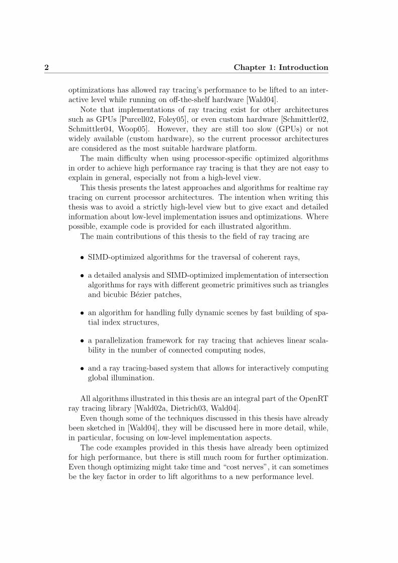
2 Chapter 1: Introduction
optimizations has allowed ray tracing’s performance to be lifted to an inter-active level while running on off-the-shelf hardware [Wald04].
Note that implementations of ray tracing exist for other architecturessuch as GPUs [Purcell02, Foley05], or even custom hardware [Schmittler02,Schmittler04, Woop05]. However, they are still too slow (GPUs) or notwidely available (custom hardware), so the current processor architecturesare considered as the most suitable hardware platform.
The main difficulty when using processor-specific optimized algorithmsin order to achieve high performance ray tracing is that they are not easy toexplain in general, especially not from a high-level view.
This thesis presents the latest approaches and algorithms for realtime raytracing on current processor architectures. The intention when writing thisthesis was to avoid a strictly high-level view but to give exact and detailedinformation about low-level implementation issues and optimizations. Wherepossible, example code is provided for each illustrated algorithm.
The main contributions of this thesis to the field of ray tracing are
• SIMD-optimized algorithms for the traversal of coherent rays,
• a detailed analysis and SIMD-optimized implementation of intersectionalgorithms for rays with different geometric primitives such as trianglesand bicubic Bezier patches,
• an algorithm for handling fully dynamic scenes by fast building of spa-tial index structures,
• a parallelization framework for ray tracing that achieves linear scala-bility in the number of connected computing nodes,
• and a ray tracing-based system that allows for interactively computingglobal illumination.
All algorithms illustrated in this thesis are an integral part of the OpenRTray tracing library [Wald02a, Dietrich03, Wald04].
Even though some of the techniques discussed in this thesis have alreadybeen sketched in [Wald04], they will be discussed here in more detail, while,in particular, focusing on low-level implementation aspects.
The code examples provided in this thesis have already been optimizedfor high performance, but there is still much room for further optimization.Even though optimizing might take time and “cost nerves”, it can sometimesbe the key factor in order to lift algorithms to a new performance level.
1.1 Outline of this thesis 3
1.1 Outline of this thesis
The thesis starts with a brief introduction to ray tracing and its use forrendering in Chapter 2. The chapter also provides a high-level performanceanalysis of the ray tracing algorithm and introduces the benefits of coherenceand CPU architecture-specific optimizations.
Chapter 3 discusses current CPU architectures in detail. As these archi-tectures build the underlying hardware platform for the implementation ofall algorithms proposed in this thesis, special emphasis is put on performanceissues and useful coding guidelines. The chapter introduces SIMD instruc-tions, which will be an essential tool for exploiting the full compute power ofcurrent CPU architectures.
Increasing ray tracing performance in particular requires an efficient traver-sal through a spatial index structure. Therefore, Chapter 4 proposes highlyoptimized algorithms for efficient traversal of coherent sets of rays. In combi-nation with optimized triangle-intersection algorithms that have been mod-ified to efficiently support coherent sets of rays, as illustrated in Chapter 5,interactive ray tracing performance for ray tracing of triangular scenes willbe achieved on a single processor.
Chapter 6 shows that interactive ray tracing is not limited to triangularscenes and presents various highly efficient intersection algorithms for bicubicBezier patches in detail. These algorithms will be discussed in depth showingtheir advantages and disadvantages in terms of performance and accuracy.
Chapter 7 demonstrates that even the construction algorithm for spatialindex structures can be efficiently optimized. A highly optimized implemen-tation in particular allows for handling fully dynamic scenes by reconstructingthe corresponding kd-tree from scratch for every frame.
Compensating the need of ray tracing for compute power means com-bining the compute power of multiple processors. Chapter 8 thus proposesa parallelization framework that effectively distributes the rendering workto a cluster of off-the-shelf PCs. As this framework has been designed forhandling high-latency interconnections, linear scalability in the number ofconnected PCs will be achieved, increasing the performance of ray-tracing toa realtime level.
If the techniques for achieving realtime ray tracing, as discussed in theprevious chapters, are combined with a global illumination algorithm thathas been exclusively modified to exploit these techniques, it becomes possibleto achieve interactive global illumination. Chapter 9 illustrates this modifiedglobal illumination algorithm and the surrounding framework.
Finally, this thesis ends with a short summary, and an outlook on thefuture of realtime ray tracing on future processor architectures.

4 Chapter 1: Introduction

Chapter 2
Introduction to Ray Tracing
This chapter starts with a brief review of the basic ray tracing algorithms(see Section 2.1) in order to provide a quick introduction to the field of highperformance ray tracing. For a more detailed introduction to the field of raytracing, please refer to one of the classical ray tracing books [Glassner89,Glassner95, Shirley03, Pharr04].
After illustrating how ray tracing is efficiently applied as a renderingalgorithm (see Section 2.2), general performance and optimization techniquesare discussed (see Section 2.3). These consolidated findings on ray tracingperformance allows better access to the role of coherence (see Section 2.4).Besides hardware-specific optimizations, coherence in all its appearances (seeSection 2.4.1 and Section 2.4.2) is the key factor for increasing ray tracingperformance to a realtime level.
2.1 The Ray Tracing Algorithm
In order to avoid confusion, the term ray tracing or core ray tracing is definedhere as an algorithm for finding the closest intersection between a ray and aset of geometric primitives, e.g. triangles [Glassner89, Badouel92, Erickson97,Moller97, Shoemake98, Shirley02, Wald04] or freeform patches [Sweeney86,Parker99b, Nishita90, Martin00, Wang01, Benthin04]. According to the rayequation R(t) = O + t ∗ D, where O is the ray origin and D the ray direction,the ray tracing algorithm returns the intersection with the smallest distancetmin ∈ [0,∞). Other ray tracing algorithms that, for example, return allintersections along a ray will not be considered in this thesis. The smallestdistance tmin ≥ 0 corresponds to the closest intersection with respect to theray origin. The actual intersection point can be easily obtained by evaluating

6 Chapter 2: Introduction to Ray Tracing
the ray equation using tmin. Note that the algorithm can easily be adapted soas to accept only intersections that lie in a given distance range [tstart, tend].
Using a brute force approach by testing all primitives within a sceneagainst the ray and comparing the resulting intersection distances, is onlyan option if the number of primitives is small. Unfortunately, the typicalnumber of primitives per scene ranges from thousands to millions makingthe brute force approach for realtime rendering impractical.
A well-known optimization technique consists in applying spatial subdivi-sion. Spatial subdivision splits the virtual scene into spatial cells and storesfor each cell the geometric primitives contained within. Note that only thoseprimitives that are contained in the spatial cells intersected by the ray needto be tested. The advantage of this approach is that only a small subsetof all spatial cells has to be considered for a given ray. Moreover, a typicalscene includes large regions of empty space, so that for most rays only asmall number of non-empty cells have to be considered. Exploiting spatialsubdivision allows for significantly reducing the required primitive tests perray, but also introduces the new problem of quickly identifying those cellsthat are intersected by the ray. The data structures required for the spatialsorting of geometry are called spatial index or spatial acceleration structures.
Algorithms for quickly identifying intersected cells are called ray traversalalgorithms. Note that only those spatial cells have to be traversed which arepierced by the ray when starting from its origin and following the ray di-rection. Keeping to such a traversal “direction” allows for efficiently findingthe closest intersection without touching any cells beyond that point. Ex-iting the traversal at the closest intersection is called early ray termination.Early ray termination can save many traversal and intersection steps (for thecells beyond the closest intersection point), but also requires a front-to-backtraversal order of all cells that are intersected by the ray.
Researchers have proposed many different spatial index structures such asbounding volume hierarchies [Rubin80, Kay86, Haines91, Smits98], uniform,non-uniform, and hierarchical grids [Fujimoto86, Amanatides87, Gigante88,Jevans89, Hsiung92, Cohen94, Klimaszewski97], octrees [Glassner84, Samet89,Cohen94, Whang95], axis-aligned BSP (binary space partitioning) trees,short kd-trees [Sung92, Subramanian90a, Bittner99, Havran01], and ray di-rection sorting techniques such as ray classification [Arvo87, Simiakakis95].These techniques either sort the primitives within a scene hierarchically(bounding volume hierarchies) or subdivide the space spanned by the prim-itives hierarchically (grids, octrees, kd-trees).
As a result, finding the closest intersection point between a ray and a setof geometric primitives includes the front-to-back traversal of a spatial indexstructure and the intersection tests for the corresponding primitives.

2.2 Ray Tracing for Rendering 7
2.2 Ray Tracing for Rendering
The core ray tracing algorithm represents the fundamental basis for many raytracing-based rendering algorithms. The common task of all these renderingalgorithms is to compute a two-dimensional image from a three-dimensionalvirtual scene. As ray tracing is well suited for accurately simulating the dis-tribution of light by simulating the propagation of photons, most ray tracing-based rendering algorithms focus on providing high image realism by closelysimulating the illumination within the virtual scene. The realism within thegenerated image largely depends on how accurately the rendering algorithmtakes into account both the illumination (by light sources) and the surfaceproperties (of the scene’s geometry). As a general rule, the higher the desiredaccuracy, the more rays have to be shot during simulation.
In order to give a better understanding of how rendering algorithms relyon the core ray tracing algorithm, a brief illustration of the standard recursiveray tracing approach [Whitted80] (see Figure 2.1) is presented next.
Generating a two-dimensional image from a three-dimensional scene us-ing recursive ray tracing comprises several steps: From a virtual camera(typically corresponding to a one-eyed imaginary observer), rays are createdand shot through each pixel of a virtual image plane. These rays are calledprimary rays, because they are created first. For each primary ray, the coreray tracing algorithm returns the closest intersection, in the following simplycalled hit or intersection point, with the geometry of the scene.
In order to determine the light at an intersection point that is reflectedin the (inverse) direction of the ray, the illumination at a given point has tobe computed first. Afterwards, the illumination must be combined with thematerial properties of the underlying geometry. The process of determiningthe interaction of light with the material properties at an intersection pointis called shading. Note that the light reflected at the intersection points ofprimary rays determines the final pixel color.
The decision of whether a light source contributes illumination to a givenhit point or not can be based on a simple occlusion test: A ray is shotfrom a hit point towards a virtual light source (or vice versa), and only ifno intersection occurs along the way, the light source will contribute to theillumination. As these rays determine whether a given hit point lies in shadowor not, they are called shadow rays. For the occlusion test itself, the core raytracing algorithm can be used once more, but it might be useful to slightlymodify the algorithm. For shadow rays, the determination of the intersectionwith the smallest distance tmin ∈ [0, distance(lightsource)] is not mandatory;instead, any intersection with a distance t ∈ [0, distance(light source)] willbe sufficient. This allows for more efficient ray termination because as soon

8 Chapter 2: Introduction to Ray Tracing
Figure 2.1: Simplified illustration for recursive ray tracing: A primary rayis generated from a virtual camera and shot through each pixel of the imageplane. The intersection closest to the ray origin is determined and testedfor illumination by the light sources (the green shadow rays). Depending onthe material properties of the intersected geometry and the incoming illumi-nation, the current intersection point is shaded and potential reflection orrefraction rays are generated. For each of these secondary rays, the contri-bution is recursively evaluated in the same way as for primary rays.
as an appropriate intersection is found, the ray tracing algorithm can beterminated.
Based on the material properties of the geometry and the underlyingrendering model, additional secondary rays can be generated to simulateeffects such as reflection or refraction. Depending on their purpose, theserays are also called reflection rays or refraction rays. The contribution ofsecondary rays to the current hit point is recursively evaluated. Even thoughthese rays are called secondary rays, they are essentially treated the sameway as primary rays.
Apart from this traditional and simple approach to recursive ray trac-ing, countless variations exists for ray tracing-based rendering [Glassner89,
2.3 Ray Tracing Performance 9
Glassner95, Shirley03]. For example, Cook extended the recursive ray tracingapproach to support additional effects such as glossy reflection, illuminationby area light sources, motion blur, and depth of field. This extended approachis called distribution ray tracing [Cook84a]. More advanced algorithms evencompute the complete global illumination within a scene, including indirectillumination and caustic effects [Cook84b, Lafortune93, Cohen93, Veach94,Veach97, Jensen01, Shirley03, Dutre03]. Even though the purpose and sup-ported accuracy of each algorithm is different, the key point is that they allheavily rely on the core ray tracing algorithm as their fundamental base.
2.3 Ray Tracing Performance
Looking at the organization of ray tracing-based rendering, it becomes clearthat all algorithms require to trace a massive number of rays. Casting onlya single primary ray per pixel at a resolution of 1024 × 1024 results in overone million rays per image. In particular, each ray must locate the correctlyintersected primitive in a scene of (typically) millions of primitives. A per-formance level that allows for generating multiple images per second requirestherefore a very fast implementation of the core ray tracing algorithm.
Section 2.1 illustrated that the core ray tracing algorithm basically con-sists of two coupled operations: traversal of a spatial index structure andray primitive intersection tests. This is why the performance of the core raytracing algorithm largely depends on the total number of required traver-sal and intersection operations. Obviously, the cost of these operations isclosely related to their implementation in terms of the underlying hardwarearchitecture.
If one has a closer look at the core ray tracing algorithm in terms ofcomputational and memory-related operations, it becomes clear that a raytraversal step mainly involves data-dependent computations. Given the cur-rent traversal state, which corresponds to a location within a spatial indexstructure, a new state (location) is computed based on the ray data and thedata loaded from the spatial index structure. As traversal states depend ondata from the spatial index structure, a data dependency exists.
For a single intersection computation, the same data dependency applies(loading primitive data from memory first, then performing intersection com-putation). However, multiple intersection tests in a given spatial cell do notdepend on each other, so that the loading of primitive data and intersectioncomputation can be interleaved or even done in parallel.
The main problem of memory-related operations is that the data accesslatency might be the limiting factor. Prior to any traversal or intersection

10 Chapter 2: Introduction to Ray Tracing
operation, the required data has to be loaded from memory first. For animplementation on a current CPU architecture, this could become criticaldue to the discrepancy between the memory latency of on-chip cache andsystem memory (a more detailed discussion will be given in Chapter 3).Ensuring a large number of data accesses to the on-chip cache is essential toachieve high performance.
2.4 Coherence
Defining the term coherence is not a trivial matter, as its meaning dependsto a great extent on the environment where it is applied. Nevertheless, thefollowing definition illustrates the term coherence in a non-restricting way:
Definition: Coherence is the degree of which parts of an environment orits projections exhibit local similarities [Foley97].
Transferring the definition of coherence into the context of ray tracing,raises the question of which parts of ray tracing exhibits local similarities. Inorder to answer this question step by step, the search for coherence is firstrestricted to the core ray tracing algorithm. Later, the search is extended tothe shading process which forms another major part of a ray tracing-basedrendering system.
2.4.1 Ray Coherence
Defining ray coherence as the degree of spatial deviation within a set of rays, astatement on coherence in the context of traversal and primitive intersectionbecomes possible.
More precisely, a set of coherent rays (see Figure 2.2) will basically travelthrough the same spatial regions, and thus access the same data of the spatialindex structure. The same holds true for the intersection test, where a setof coherent rays will basically test similar primitives. As a result, one candefine traversal coherence for a set of rays as the ratio between the numberof spatial cells traversed by all rays (as entity) and the sum of cells traversedby any ray. In the same manner, one can define intersection coherence for aset of rays as the ratio between the number of intersection tests performedby all rays (as entity) and the number of intersection tests performed by anyrays.
The higher the traversal and intersection coherence the higher the prob-ability of loading the same data, exploiting the memory cache hierarchy ofcurrent CPU architectures. In this case, traversal and intersection coherencetranslate into memory coherence.
2.4 Coherence 11
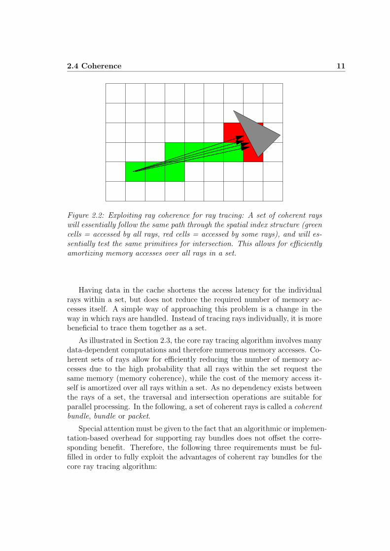
Figure 2.2: Exploiting ray coherence for ray tracing: A set of coherent rayswill essentially follow the same path through the spatial index structure (greencells = accessed by all rays, red cells = accessed by some rays), and will es-sentially test the same primitives for intersection. This allows for efficientlyamortizing memory accesses over all rays in a set.
Having data in the cache shortens the access latency for the individualrays within a set, but does not reduce the required number of memory ac-cesses itself. A simple way of approaching this problem is a change in theway in which rays are handled. Instead of tracing rays individually, it is morebeneficial to trace them together as a set.
As illustrated in Section 2.3, the core ray tracing algorithm involves manydata-dependent computations and therefore numerous memory accesses. Co-herent sets of rays allow for efficiently reducing the number of memory ac-cesses due to the high probability that all rays within the set request thesame memory (memory coherence), while the cost of the memory access it-self is amortized over all rays within a set. As no dependency exists betweenthe rays of a set, the traversal and intersection operations are suitable forparallel processing. In the following, a set of coherent rays is called a coherentbundle, bundle or packet.
Special attention must be given to the fact that an algorithmic or implemen-tation-based overhead for supporting ray bundles does not offset the corre-sponding benefit. Therefore, the following three requirements must be ful-filled in order to fully exploit the advantages of coherent ray bundles for thecore ray tracing algorithm:
12 Chapter 2: Introduction to Ray Tracing
Spatial Index Structure: The spatial index structure and the correspond-ing traversal algorithm must efficiently support ray bundles. The traver-sal algorithm in particular should avoid any complex computations.
Ray Bundle Traversal: An implementation of ray bundle traversal (withrespect to a chosen spatial index structure) must minimize any overheaddue to inefficient mapping to the underlying hardware architecture.Ideally, the hardware architecture and its corresponding instructionset should optimally support an implementation.
Ray Bundle Intersection: Similar to a traversal implementation, an in-tersection implementation has to efficiently support ray bundles. Asdifferent types of geometric primitives can exist in the same scene, raybundle intersection algorithms should efficiently support various prim-itive types.
In the case no efficient ray bundle intersection algorithm can be foundfor a given primitive type, the fall-back solution of intersecting the rayssequentially might be acceptable.
Chapters 4, 5, and 6 will provide a detailed discussion of data structures,algorithms, and the corresponding implementations that fulfill all these re-quirements.
2.4.2 Shading Coherence
Besides the actual core ray tracing algorithm, the shading process also ben-efits from local similarities. Considering for example the hit points of neigh-boring primary rays which are likely to intersect the same primitive. Even ifthis is not the case, it is very likely that the hit points are in the same spatialregion. In addition, the probability that the intersection points share thesame shader, and therefore perform similar shading operations is very high.Similar shading operations could be performed in parallel, again allowing forprocessing the shading of intersection points in bundles.
Sharing the same shader implies additionally that the loaded data exhibitssimilarities as well. For example, look-ups to the same texture for neighboringintersection points are likely to provide a high degree of memory coherence,which in turn allows for the efficient use of caches.
As a result, the shading process itself can benefit from coherence; however,similar to the core ray tracing algorithm, bundle shading for intersectionpoints is prone to overhead caused by inefficient implementation.

2.5 Conclusions 13
2.5 Conclusions
This chapter has demonstrated that the key to pushing ray tracing per-formance to a realtime level is an efficient support of coherent ray bundlescombined with a highly optimized implementation. A sub-optimal implemen-tation in particular is likely to offset any benefit offered by tracing bundles.Unfortunately, current CPU architectures in combination with their support-ing compilers are not intended to support the required degree of efficiency outof the box. On the contrary, without any manual effort in optimizing algo-rithms and implementation code, there is only little chance of ever reachingthe desired performance level.
In order to avoid hardware and software-specific implementation pitfalls,it is beneficial to examine the architecture of current CPUs more closely(see Chapter 3). Taking specific CPU-related issues into account allows foran efficient implementation of the core ray tracing algorithm. In particular,the optimized implementation includes the extension of the traversal algo-rithm (see Chapter 4) and the primitive intersection tests (see Chapter 5 andChapter 6) for efficiently supporting ray bundles.
A difficult task for a ray tracing-based rendering system is to gather co-herent ray bundles. Coherent bundles of primary rays can easily be generatedwhen relying on a typical (perspective) camera model, where primary rays ofneighboring pixels exhibit a large degree of coherence. The same holds truefor the shadow rays generated towards a single point on a light source. How-ever, for most secondary rays, e.g. those generated by reflection off of curvedsurfaces and even refraction rays, coherence will be significantly lower thanfor primary rays. In the case of low coherence, coherence-based regroupingor even falling back to tracing individual rays may be necessary.
Instead of trying to extract coherent ray bundles out of a traditional raytracing-based rendering system, one can design the rendering system in sucha way that the majority of rays can be combined directly in coherent bun-dles (see Chapter 9). Such a system allows for minimizing the overhead forgenerating coherent bundles. If for such a system the majority of renderingtime is spent in the core ray tracing algorithm, total system performance willdirectly benefit from fast ray bundle tracing.

14 Chapter 2: Introduction to Ray Tracing

Chapter 3
CPU Architectures
Optimizing program code basically consists of two steps: Identifying theprogram’s hot spots and trying to modify the corresponding code sequences.The difficulty thereby is to modify the code in such a way that the modi-fied version shows better run-time behavior (with respect to the underlyinghardware architecture) than the original one. This requires identifying codestructures that cannot be efficiently executed. Identifying and modifyingmakes code optimization a difficult and time-consuming task which requiresin-depth knowledge of the underlying architecture. Apart from architecturalissues, code optimization additionally depends on the chosen compiler.
Nevertheless, the benefits of code optimization can be tremendous. Statis-tics have shown that the increase in performance between optimized and non-optimized code can range from a few percent to entire orders of magnitude.
In order to avoid costly performance penalties in critical code sequences,it is essential to have a detailed knowledge of the execution flow within theunderlying CPU architecture. Therefore, a brief overview of performance-related issues of today’s CPU architectures will be given in Section 3.1.Having identified the architecture related issues allows for formulating thegeneral coding guidelines of Section 3.2. Section 3.3 introduces the conceptof SIMD instructions, while Section 3.4 discusses compiler and performanceprofiling-related tools.
3.1 Performance Issues
For historical reasons, the majority of today’s software has been designedfor non-parallel execution. Because of this, current CPU architectures aredesigned to execute serial program code as fast a possible. With every newCPU generation, designers have tried to achieve a continuous performance

16 Chapter 3: CPU Architectures
increase by introducing small architectural enhancements to optimize serialexecution. The key factor to increase performance has been the raising ofthe CPU clock rate (up to 3.8 GHz for latest Pentium-IV [Intel01]). Hav-ing a higher clock rate allows for (potentially) executing more instructionswithin a fixed time period. Raising the clock rate could only be realizedthrough smaller micro structure designs which require extremely long exe-cuting pipelines (the Pentium-IV uses a pipeline with more than 30 stages).
These long executing pipelines are the major drawback of the high clockrate architectures. If the utilization of the execution pipeline is low, theperformance of the CPU itself will be low, too. Even though the analysisand optimization of execution bottlenecks is a quite complex topic, the mainreasons for low pipeline utilization, and thus low performance, can be roughlyclassified into the following categories:
Cache Misses: The difference in access latency between on-chip memorycache and main memory itself is tremendous, e.g. the Pentium-IV hasan L1 cache latency of 1-4 cycles, an L2 cache latency of 20-27 cy-cles, and a latency to main memory of over 200-300 cycles. Obviously,this can result in pipeline stalls whenever data does not reside in thememory cache hierarchy. CPU architectures follow multiple ways ofreducing the impact of cache misses by having large and multiple cachelevels to reduce the probability of cache misses, and by executing in-dependent program code during idle periods. For serial program code,the search for, and the execution of, independent instructions is oftenreferred to as out-of-order execution. On the other hand, techniquessuch as simultaneous multi-threading or hyper-threading [Intel02c] usethe implicit parallelism of thread execution to fill pipeline stalls withindependent instructions.
Branches: The negative impact of long executing pipelines comes into playwhen dealing with conditional branches. Every time a branch is wronglypredicted, the complete pipeline has to be flushed. Branch prediction(over multiple levels) and even branch prediction by branch hint in-structions are able to lower the probability. Nevertheless, every mis-predicted branch means a “waste” of up to 30 cycles for a 30-stageexecution pipeline. Even though the negative performance impact islower than for cache misses it is still significant. This particularly af-fects complex and branch-intensive code.
Low Instruction Level Parallelism: Multiple instruction pipelines andfunctional units combined with out-of-order execution even allow theserially operating CPU to execute multiple independent instructions in
3.1 Performance Issues 17
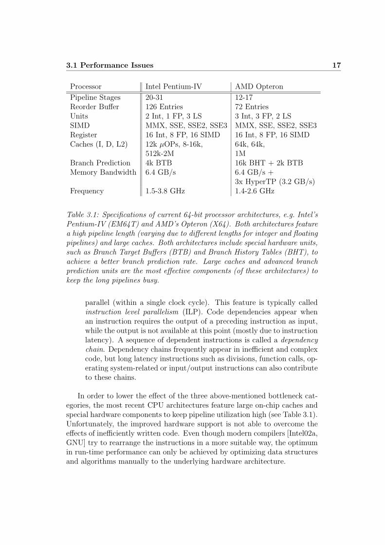
Processor Intel Pentium-IV AMD Opteron
Pipeline Stages 20-31 12-17Reorder Buffer 126 Entries 72 EntriesUnits 2 Int, 1 FP, 3 LS 3 Int, 3 FP, 2 LSSIMD MMX, SSE, SSE2, SSE3 MMX, SSE, SSE2, SSE3Register 16 Int, 8 FP, 16 SIMD 16 Int, 8 FP, 16 SIMDCaches (I, D, L2) 12k µOPs, 8-16k, 64k, 64k,
512k-2M 1MBranch Prediction 4k BTB 16k BHT + 2k BTBMemory Bandwidth 6.4 GB/s 6.4 GB/s +
3x HyperTP (3.2 GB/s)Frequency 1.5-3.8 GHz 1.4-2.6 GHz
Table 3.1: Specifications of current 64-bit processor architectures, e.g. Intel’sPentium-IV (EM64T) and AMD’s Opteron (X64). Both architectures featurea high pipeline length (varying due to different lengths for integer and floatingpipelines) and large caches. Both architectures include special hardware units,such as Branch Target Buffers (BTB) and Branch History Tables (BHT), toachieve a better branch prediction rate. Large caches and advanced branchprediction units are the most effective components (of these architectures) tokeep the long pipelines busy.
parallel (within a single clock cycle). This feature is typically calledinstruction level parallelism (ILP). Code dependencies appear whenan instruction requires the output of a preceding instruction as input,while the output is not available at this point (mostly due to instructionlatency). A sequence of dependent instructions is called a dependencychain. Dependency chains frequently appear in inefficient and complexcode, but long latency instructions such as divisions, function calls, op-erating system-related or input/output instructions can also contributeto these chains.
In order to lower the effect of the three above-mentioned bottleneck cat-egories, the most recent CPU architectures feature large on-chip caches andspecial hardware components to keep pipeline utilization high (see Table 3.1).Unfortunately, the improved hardware support is not able to overcome theeffects of inefficiently written code. Even though modern compilers [Intel02a,GNU] try to rearrange the instructions in a more suitable way, the optimumin run-time performance can only be achieved by optimizing data structuresand algorithms manually to the underlying hardware architecture.

18 Chapter 3: CPU Architectures
The road map of the leading CPU manufacturers makes it clear thatthe length of the pipeline, and thus the frequency of future CPUs is notlikely to grow significantly, and may even decrease. Therefore, future CPUdesigns will rely on increased execution parallelism such as multiple pipelinesand functional units, execution threads, and in particular many cores inorder to increase performance. Introducing multiple cores will widen the gapbetween memory latency/bandwidth and compute power dramatically. Aseach core will access the main memory via the same memory interconnect,future algorithms will need to reduce their required memory bandwidth.
3.2 Coding Guidelines
The performance impact of inefficiently written code ranges from a few per-cent to entire orders of magnitude, largely depending on the code itself. Eventhough the following coding guidelines seem obvious, it is worth outliningthem to reduce the probability of significant performance penalties:
Data Locality and Memory Access Pattern: Localizing memory accessensures high cache hit probability. In situations where large chunks ofmemory need to be loaded, a qualified memory access pattern suchas pure sequential access should be applied. Sequential access is ef-ficiently supported by the hardware prefetching unit, available on allcurrent CPU architectures. In certain situations, it is beneficial tomanually apply CPU-supported prefetch instructions in order to loadchunks of memory in advance. As memory prefetching is done asyn-chronously to the execution flow, the loading latency can be hidden byworking on data already residing in the cache hierarchy. Obviously, themechanism only works if the memory loading latency is smaller thanthe computation time between subsequent prefetches.
Simple Control Flow: Replacing branch-frequent code by conditional movesequences avoids mis-predicted branches. However, if the probabilityof a branch mis-prediction is sufficiently low (something which dependslargely on the code), applying branches can be faster than applying con-ditional moves, because the execution of a correctly predicted branchhas almost no costs. In contrast, conditional move sequences may re-quire the computation of results which may not even be used later. Ona more higher level, critical run-time loops should be kept as small andas simple as possible. Simply dropping or replacing complex instruc-tions such as divisions or functions calls in inner loops can dramaticallyspeed up performance. Having only a minimum of code dependency

3.3 Data Level Parallelism by SIMD Instructions 19
chains within the inner-most loop body can additionally increase in-struction throughput. Furthermore, small and simple inner-loops canbe more easily optimized and maintained.
Data Level Parallelism: In order to maximize performance, data levelparallelism by SIMD (single instruction multiple data) instructionsshould be applied. SIMD instructions offer a simple and easy wayto manipulate multiple data elements at once. In particular, Intel’sSSE instruction set [Intel01, Intel02b, Intel02a] allows for manipulat-ing four single precision floating point or integer values using a singleinstruction. The main issues when using SIMD instructions are the re-quired layout changes of input data and the necessary recoding of thealgorithm (see Section 3.3).
Data level parallelism via SIMD instructions is currently the only wayof explicitly performing parallel operations on a sequentially operating CPU(see Section 3.3). Instruction level parallelism, on the other hand, is per-formed internally by the CPU (out-of-order execution). It can only be in-fluenced implicitly by reordering code for a more appropriate out-of-orderexecuting flow.
In contrast to single-threaded applications, coding guidelines for multi-threaded applications should also contain guidelines for thread synchroniza-tion. In order to efficiently exploit multiple CPUs (or CPU cores), syn-chronization points (such as mutex lock/unlocks [Nichols96]) should be keptto a minimum. Roughly speaking, synchronization means serialization, andlong serialization periods dramatically reduce the positive effect of parallelexecution.
Multi-threaded performance is further affected whenever implicit synchro-nization is required. Implicit synchronization occurs when caches on differ-ent CPUs need to be synchronized. Even though the interconnects betweenCPUs offer a high bandwidth for synchronizing cache areas, the performanceimpact can still be very high. Due to the fact that the synchronizationgranularity is based on cache-lines, unintended cache synchronization can beavoided by assuring that synchronization-relevant data exclusively occupiescomplete cache-lines.
3.3 Data Level Parallelism by SIMD Instructions
The basic concept behind SIMD instructions is the idea that many algorithms(see Figure 3.1) could work on multiple data elements in parallel. Instead ofprocessing each data element by a single instruction in a sequential manner,

20 Chapter 3: CPU Architectures
// the four three-component input vectors are
// stored in the SOA format.
//
// float x[4] -> the four ’x’ vector components
// float y[4] -> the four ’y’ vector components
// float z[4] -> the four ’z’ vector components
inline void SimpleDot4(const float *x,
const float *y,
const float *z,
float *const dest)
{
dest[0] = x[0]*x[0]+y[0]*y[0]+z[0]*z[0];
dest[1] = x[1]*x[1]+y[1]*y[1]+z[1]*z[1];
dest[2] = x[2]*x[2]+y[2]*y[2]+z[2]*z[2];
dest[3] = x[3]*x[3]+y[3]*y[3]+z[3]*z[3];
}
Figure 3.1: Computing a dot product of four three-component floating pointvectors with standard C/C++ code. As no dependencies exists, the compu-tation (for each component of ’dest’) can be performed in parallel. Note thatthe code does not implement a generic dot product, but rather a simplifiedversion where only one input vector is used for both dot product elements.
one could apply the same operation to multiple elements in parallel using asingle instruction.
Applying SIMD requires that no dependencies exist between the dataelements in a processing group. Moreover, controlling program executionby conditional branches brings about certain changes: Instead of basing thebranch on the result of a single condition, SIMD instructions compute theresults of multiple conditions in parallel. Obviously, one could extract theresult of a single condition and perform the branch with respect to it, butvery often it is more beneficial to perform the branch based on a conditionregarding all results.
SIMD features are available on almost all current processor architec-tures [Intel02b, AMD03, AltiVec, IBM05], but only Intel’s Streaming SIMDExtension will be considered in the following. Nevertheless, all code examplesin this thesis can be easily ported to a different SIMD extension.
3.3.1 Intel’s Streaming SIMD Extension (SSE)
For historical reasons, floating point operations on x86 architectures havebeen executed using the FPU (floating point unit). FPU registers have been
3.3 Data Level Parallelism by SIMD Instructions 21
organized in a stack-like structure, causing reorganization overhead for exe-cuting floating point operations. With the introduction of the Pentium-III,Intel for the first time offered SIMD features with its Streaming SIMD Ex-tension (SSE) [Intel02b].
1 2 3
3210
00 1 1 2 2 3 3
X X X XYYYY
X+Y X Y+ X+Y X+Y
0 xmm0
xmm1
addps xmm0,xmm1
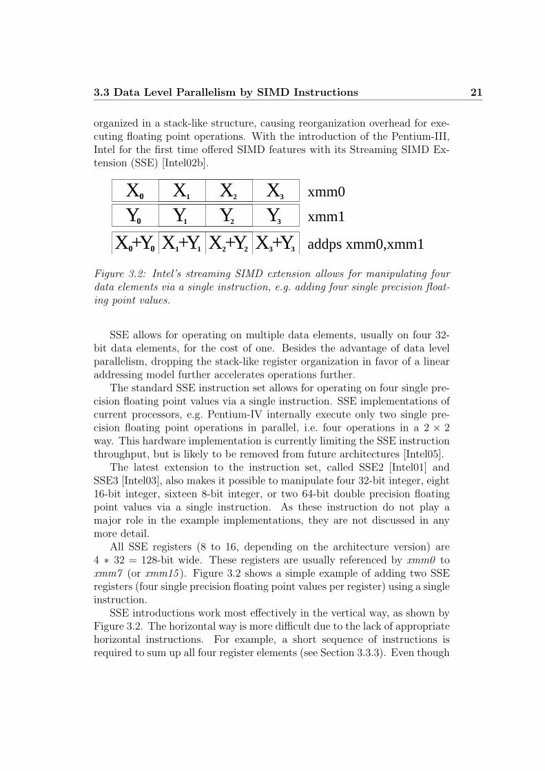
Figure 3.2: Intel’s streaming SIMD extension allows for manipulating fourdata elements via a single instruction, e.g. adding four single precision float-ing point values.
SSE allows for operating on multiple data elements, usually on four 32-bit data elements, for the cost of one. Besides the advantage of data levelparallelism, dropping the stack-like register organization in favor of a linearaddressing model further accelerates operations further.
The standard SSE instruction set allows for operating on four single pre-cision floating point values via a single instruction. SSE implementations ofcurrent processors, e.g. Pentium-IV internally execute only two single pre-cision floating point operations in parallel, i.e. four operations in a 2 × 2way. This hardware implementation is currently limiting the SSE instructionthroughput, but is likely to be removed from future architectures [Intel05].
The latest extension to the instruction set, called SSE2 [Intel01] andSSE3 [Intel03], also makes it possible to manipulate four 32-bit integer, eight16-bit integer, sixteen 8-bit integer, or two 64-bit double precision floatingpoint values via a single instruction. As these instruction do not play amajor role in the example implementations, they are not discussed in anymore detail.
All SSE registers (8 to 16, depending on the architecture version) are4 ∗ 32 = 128-bit wide. These registers are usually referenced by xmm0 toxmm7 (or xmm15 ). Figure 3.2 shows a simple example of adding two SSEregisters (four single precision floating point values per register) using a singleinstruction.
SSE introductions work most effectively in the vertical way, as shown byFigure 3.2. The horizontal way is more difficult due to the lack of appropriatehorizontal instructions. For example, a short sequence of instructions isrequired to sum up all four register elements (see Section 3.3.3). Even though

22 Chapter 3: CPU Architectures
the latest architectures [Intel03] offer direct support for horizontal operations,they are not as efficient implemented as vertical operating instructions.
0 0 0 0
0
0
1 1 1
1
1
12 2 2
2
2
2
3 3 3
3
3
3
X Y Z
X Y Z
−
−
−
−
ZYX
X Y Z
X X X X
Y Y Y Y
ZZZZ
Figure 3.3: Left: For many algorithms, e.g. computing dot products, thestandard array-of-structure (AOS) layout does not ensure optimal SSE uti-lization (the right-most element is not used). Right: The structure-of-array(SOA) layout is more beneficial as it optimally supports vertically operatingSSE instructions.
As a consequence, the layout of data and the implementation of algo-rithms should be rearranged to allow for as many vertical instructions aspossible. As an example, vertex data should be stored in the structure-of-array (SOA) format instead of the array-of-structure (AOS ) format (seeFigure 3.3). Figure 3.4 shows that using the structure-of-array data layout,four dot products can be efficiently implemented by using only five instruc-tions. The array-of-structure data layout would require more than doublethe number of instructions (because of the required shuffle operations).
0
0
0
1
1
1
2
2
2
3
3
3
xmm0X X X XY Y Y Y
ZZZZxmm1
xmm2
mulps xmm0,xmm0mulps xmm1,xmm1mulps xmm2,xmm2addps xmm0,xmm1addps xmm0,xmm2
Figure 3.4: The structure-of-array (SOA) data layout allows for efficientlyusing SSE instructions, e.g. computing four (simple) dot products in parallel(similar to the code in Figure 3.1) using only 5 instructions.

3.3 Data Level Parallelism by SIMD Instructions 23
If the array-of-structure layout as input format cannot be avoided, a cor-responding transposition into the structure-of-array can be performed on-the-fly. The transposition code consists of a sequence of shuffle and loadinstructions. The decision of whether the overhead introduced by the re-arrangement of register elements is tolerable or not largely depends on thecode. If the code following the transposition is sufficiently long, the intro-duced overhead can be effectively amortized.
Another important factor concerning efficient coding with SSE instruc-tions relates to the rearrangement of instructions in terms of their throughputand latency. In particular, conditional branches based on a comparison be-tween SSE registers require a manual transfer of the resulting bit mask (seeSection 3.3.2) from an SSE register to a general purpose register. This trans-fer suffers from an high latency and should therefore be used carefully. Onthe other hand, coding in terms of instruction throughput is essential foravoiding resource conflicts of computational units. Throughput and latencyvary across x86 architectures (and their variants), making general codingoptimizations difficult. Fortunately, modern compilers allow for reorderingcode with respect to a specific processor without much manual effort.
Another important limitation of SSE instructions is the lack of scat-ter/gather operations for loading and storing data. Loading or storing indi-vidual register elements requires a sequence of loading and shuffle operations,because only the lowest register element can be handled as a standard scalarregister.
3.3.2 SSE Intrinsics
One possible way to benefit from SSE instructions is to directly rely on assem-bly programming, but this procedure would be too inflexible and error-prone.On the other hand, modern C/C++ compilers (see Section 3.4) offer auto-vectorization of standard C/C++ program code. Even though this allowsfor programming in standard C/C++ code, the output typically will notreach the quality of hand-written code. Furthermore, the compilers oftenfail to auto-vectorize loops because of unresolvable dependencies (from thecompiler’s view) within the loop body. A more efficient way that combinesboth the quality of hand-written assembly code and the high-level inter-face of C/C++ code are SSE intrinsics [Intel02a]. Intrinsics are C/C++function-style macros, which can be used directly with C/C++ constructsand variables. During compilation, the compiler automatically takes care ofregister allocation, result propagation, intermediate usage, etc.
Due to the fact that the compiler takes care of SSE register and memoryallocation, the programmer can focus on the algorithmic implementation

24 Chapter 3: CPU Architectures
// the four three-component input vectors are stored
// in the SOA format using a SIMD vector data type.
//
// u[0] -> the four ’x’ vector components
// u[1] -> the four ’y’ vector components
// u[2] -> the four ’z’ vector components
typedef typedef __m128 sse_t;
inline sse_t SimpleDot4SSE(const sse_t *u)
{
return _mm_add_ps(_mm_add_ps(_mm_mul_ps(u[0],u[0]),
_mm_mul_ps(u[1],u[1])),
_mm_mul_ps(u[2],u[2]));
}
Figure 3.5: Intrinsics allow for effectively using SIMD instructions withC/C++ constructs. This small routine computes four (simple) dot products(similar to the code in Figure 3.1) in parallel using SSE intrinsics.
itself (see Figure 3.5). Moreover, the compiler is able to perform architecture-specific optimizations, e.g. considering throughput and latency optimizations.Most SSE intrinsics map to a single SSE instruction, others are composed ofa short sequence of SSE instructions.
Given the importance of SSE instructions for efficient coding, the mostfrequently used instructions will be discussed in more detail. Note that scalaroperating intrinsics, operating only on the lowest register element, differ fromtheir full counterpart only through the ss-suffix instead of the ps-suffix.
Arithmetic Instructions For addition, multiplication, subtraction, and di-vision of four single precision floating point values, the intrinsics mm add ps,mm mul ps, mm sub ps, mm div ps are used. Reciprocal operations arealso useful, e.g. mm rcp ps and mm rsqrt ps, which perform the 1/x and1/sqrt(x) operations. These special instructions are faster than a real di-vision or square root. The speed increase comes at the expense of reducedaccuracy because the result is computed based on approximating algorithms.Nevertheless, the reduced accuracy can be increased afterwards by perform-ing a Newton-Raphson iteration [Intel02b] (resulting in a short sequence ofadditional instructions). Breaking up costly long-latency instructions suchas real divisions or square roots into a short sequence of short-latency in-structions is more advantageous for exploiting instruction level parallelism.
3.3 Data Level Parallelism by SIMD Instructions 25
Load/Store Instructions Loading one single or four single precision float-ing point values can be performed using the intrinsics mm load ss andmm load ps. Note that the argument of mm load ss and mm load ps is apointer to a float or float array. Additionally, mm load ps requires that theaddress is aligned on a 16-byte boundary to ensure maximum performance(less efficient non-aligned access can be implemented by mm loadu ps). Theintrinsics mm set ps and mm set ps1 use immediate float values as argu-ments. mm set ps1 copies a single value into all four register elements.Note that loading four different float values into a single register by applyingmm set ps and mm rset ps involves a sequence of shuffle instructions. Re-turning the lowest SSE register element as scalar float value can be performedby using the mm cvtss f32 intrinsic.
Comparison Instructions Comparisons between two SSE registers usingthe mm cmpXX ps (XX can be eq,lt,gt,...) return a mask where all bits ofeach register element are set to one if the result of the comparison is trueand are set to zero otherwise. In combination with a sequence of logicalinstructions, the returned bit mask can be used to implement an element-based conditional move sequence.
Miscellaneous Instructions The mm shuffle ps intrinsic shuffles registerelements within one single or across two registers (with certain restrictions).It is often necessary to apply a conditional jump based on the values ofall four register elements. Therefore, mm movemask ps transfers the high-est bit (the sign bit) of each register element to the four lowest bits of ageneral purpose register. If all register elements contain a comparison’s bitmask, the transferred bits correspond to the comparison result. In order toquickly obtain the maximum and minimum values per register element, themm max ps and mm min ps intrinsics can be used.
Logical Instructions The logical operations or, and, xor, and notandare realized by mm or ps, mm and ps, mm xor ps, and mm andnot ps.mm setzero ps allows for quickly setting all register elements to zero usinga simple xor operation.
3.3.3 Using Intrinsics and Basic Data Structures
As discussed in Section 3.2, the performance impact of mis-predicted branchesdue to pipeline flushes can be critical. This holds especially true for SSEcode sequences. In many cases, a conditional branch construct looks like:

26 Chapter 3: CPU Architectures
IF condition THEN C=A ELSE C=B. An efficient way to realize these if-else-constructs per SSE register element without branching is to apply bitmasking (returned by an SSE-comparison) using a short sequence of logicalinstructions (see Figure 3.6).
inline sse_t Update4(const sse_t a, const sse_t b, const sse_t mask)
{
// note that ’andnot’ requires the ’mask’ as first parameter
return _mm_or_ps(_mm_and_ps(a,mask),
_mm_andnot_ps(mask,b));
}
Figure 3.6: Small utility functions increase the readability of SSE code signif-icantly. The routine implements an - IF condition THEN C=A ELSE C=B- construct on register element level.
For the operation of computing the inverse of four single precision valuesin parallel, it is often beneficial to not apply a real division, but to usea reciprocal approximation combined with a Newton-Raphson iteration inorder to increase the result’s accuracy later on. Figure 3.7 shows the actualSSE implementation.
inline sse_t Inverse4(const sse_t n)
{
const sse_t rcp = _mm_rcp_ps(n);
return _mm_sub_ps(_mm_add_ps(rcp,rcp),
_mm_mul_ps(_mm_mul_ps(rcp,rcp),n));
}
Figure 3.7: Fast inverse computation by using reciprocal approximation com-bined with a Newton-Raphson step in order to increase IEEE precision to 24bits. In many cases, splitting up inverse computation into multiple instruc-tions is faster than using an explicit division, because the instruction levelparallelism of current CPUs allows for a efficient parallel execution with sur-rounding instructions.
Up to the latest Pentium-IV [Intel03] and Opteron processor generations,SSE instructions have been lacking direct hardware support for horizontaloperations. Horizontal operations work on all elements of a single registerand store the result in the lowest element. However, horizontal operationscan be simulated using a sequence of instructions. As shown in Figure 3.8,a horizontal add requires at least four instructions. Similar utility functionscompute horizontal sub, min, and max operations.

3.4 Tools and Hardware 27
inline sse_t sseHorizontalAdd(const sse_t &a)
{
const sse_t ftemp = _mm_add_ps(a, _mm_movehl_ps(a, a));
return _mm_add_ss(ftemp,_mm_shuffle_ps(ftemp, ftemp, 1));
}
Figure 3.8: Many architectures do not offer SSE instructions for perform-ing horizontal operations, e.g. adding all four register elements and storingthe result in the lowest element. Instead, a short sequence of instructionsemulates these horizontal operations.
Given the seamless integration of intrinsics into C/C++ code, it is ben-eficial to implement useful code sequence as small utility functions. Theseutility functions increase the readability of the SSE code significantly.
Another important point to consider is the fact that even coherence ishighly important for implementing algorithms through SSE code. This is es-pecially true for conditional branching based on the values of all four registerelements (using the mm movemask ps instruction). In this case, decision-coherence which is defined as the probability that the comparison result in allfour register elements is equal, is essential. Testing the sixteen possibilitiesby if-else or switch statements, where each case has equal probability, wouldtypically result in many branch mis-predictions. Therefore, a high decision-coherence allows for arranging the comparison statements based on theirprobability. This efficiently reduces the amount of mis-predicted conditionalbranches.
Creating fundamental data structures for tracing ray bundles is straight-forward. Due to the fact that SSE operates on four elements at once, struc-tures for storing information of four rays are created first. Figure 3.9 showsdata structures for storing four three-component vectors in the SOA format,and the hence constructed four-ray structure.
Besides a structure for ray and intersection data, a structure for axis-aligned bounding boxes, e.g. as representation for spatial voxels, is oftenrequired. An efficient representation based on the extremal expansion isshown in Figure 3.10.
3.4 Tools and Hardware
Because of the required SSE intrinsics support, all algorithms were imple-mented using either the GCC compiler collection [GNU] or the Intel C/C++compiler suite [Intel02a]. Because of its superior performance, the Intel com-

28 Chapter 3: CPU Architectures
struct R3 {
float x,y,z;
};
// -- single ray --
struct Ray {
R3 direction;
R3 origin;
};
struct Intersection {
float dist;
float u;
float v;
float id;
};
// -- packet/bundle of four rays --
struct SSEVec4 {
sse_t t[3]; // SOA format
};
struct SSERay4 {
SSEVec4 direction;
SSEVec4 origin;
};
struct SSEIntersection4 {
sse_t dist;
sse_t u;
sse_t v;
int id[4];
};
Figure 3.9: ’R3’ is the basic representation of a three-component vector,while ’Ray’ and ’Intersection’ store ray and intersection data for a single ray.’SSEVec4’ is the fundamental data structure for storing four three-componentvectors in the SOA format. It builds the base for the ’SSERay4’ structure,which stores the data for four rays. The ’SSEIntersection4’ structure storesthe data for four intersection points, e.g. intersection distance, barycentriccoordinates, and the index of the primitive hit.
piler is favored over the standard GCC compiler. It is interesting to see thatthe Intel compiler creates very efficient code not only for Intel processors,but also for its competitors.
For profiling, analyzing, and identifying code bottlenecks, the VTuneprofiling tool is used [Intel04]. The tool provides a detailed analysis fordetecting performance-related bottlenecks caused by cache misses, branch

3.5 Conclusions 29
struct Box {
R3 min;
float dummy0;
R3 max;
float dummy1;
};
Figure 3.10: Structures for representing three-component vectors and axis-aligned bounding boxes. The axis-aligned bounding box is represented by theirextremal points. The additional dummy values ’dummy0’ and ’dummy1’ in-crease the total structure to a preferable size of 32 bytes, which is more suit-able with respect to cache-line sizes. Note that no SSE data types are usedbecause for many algorithms a fast access to individual vector elements mustbe ensured (avoiding the overhead for accessing SSE register elements). Inthe two dummy values additional information can be stored.
mis-predictions, etc. Furthermore, VTune provides many useful statisticssuch as cycles per instructions ratios, issued/retired ratios with respect todifferent instruction types, etc.
For providing an approximate cost measure for a short code sequence,the internal processor’s clock cycle counter [Intel97] is used. Note that out-of-order execution, caching effects, varying branch table history entries, sur-rounding code sequences, and even differences in the underlying architecturemake it very difficult to determine the exact amount of cycles required for agiven code sequence. Therefore, all cycle statistics in this thesis should beseen as estimates rather than exact values.
As operating system a 32-bit or 64-bit Linux distribution, running a 2.4kernel has been used. Most of the performance statistics were measuredon a 2.2 GHz Pentium-IV PC with 512 MB of memory. In a few cases,in particular where a PC cluster setup was needed, a cluster of PCs withAthlonMP 1800+ PCs (running at 1.5 GHz) was used. Whenever a 64-bitprocessor provided superior performance compared to a 32-bit processor, a64-bit AMD Opteron PC with 1.8 GHz has been chosen.
3.5 Conclusions
Current CPU architectures are able to provide a large amount of computingpower if they execute well-suited code. Even though today’s compilers offerautomatic optimization features, the full potential of a processor can only beutilized by manual optimization.

30 Chapter 3: CPU Architectures
The difference in performance between manually optimized and unopti-mized code can reach order of magnitudes. Therefore, it will become moreand more important to focus on the optimization of critical code sections. Itcan even be beneficial to favor algorithms that have a sub-optimal algorithmiccomplexity, but allow for very simple and therefore fast implementation. Animplementation requiring only a sequence of simple instructions is typicallymore suited for current CPU architectures.
Apart from simplicity of implementation, the memory access pattern ofalgorithms is another critical point. Code that is optimized to access memoryin a cache-friendly way is likely to outperform unoptimized code. The sameoptimization argument holds true for branch and ILP optimizations.
As a result, it is essential for achieving optimal performance on currentCPU architectures to carefully chose and optimize algorithms in terms of theunderlying architecture.
Chapter 4
Tracing Coherent Ray Bundles
Efficiently searching for the first intersection along a ray requires building upa spatial index structure over the primitives within the scene. The spatialcells created by the spatial index structure allow for efficiently reducing thenumber of potential intersection candidates but require a way of quicklyidentifying those cells that are intersected by the ray. Moreover, the cellshave to be traversed in front-to-back order to ensure early ray termination.
The spatial index structure has a tremendous impact on the performanceof the core ray tracing algorithm. The following issues describe those impactsin detail:
Quality: The quality of a spatial index structure is measured in terms of thenumber of required traversal steps versus resulting intersection opera-tions. Depending on the chosen index structure and the correspondingimplementation, it can be beneficial to increase the required numberof operations of one category in order to decrease the number of oper-ations of the other category, i.e. to have a higher number of traversaloperations in order to perform fewer intersection operations. Never-theless, the main goal should be to reduce the number of operations inboth categories.
Memory Layout: The larger the memory representation of a spatial in-dex structure the higher the required bandwidth to memory. In thecase the processor’s cache hierarchy is not able to efficiently supportmemory accesses to the spatial index structure, the core ray tracingalgorithm can easily become memory-bandwidth limited. Moreover, asub-optimal memory access pattern (e.g. accessing data crossing cache-lines) or a too complex data extraction sequence (e.g. decompressingspatial cell data) can significantly impact performance.

32 Chapter 4: Tracing Coherent Ray Bundles
Traversal Costs: Besides the number of traversal steps, the cost of per-forming a single traversal step for one or more rays is particularly im-portant. Complex code that does not efficiently map to the underlyinghardware architecture is able to offset any benefit from a high-qualityspatial index structure.
Apart from quality and memory requirements, the traversal operationmust be generalizable for efficiently supporting coherent ray bundles (seeSection 2.4.1), because this has turned out to be one of the key factors forpushing ray tracing performance [Wald04, Reshetov05]. This means thatdata access costs can be efficiently amortized over all rays within the bundle(instead of only one ray at a time). This allows for reducing the requiredmemory bandwidth, which is known to be one of the major bottlenecks ofcurrent CPU architectures. Since a traversal operation is performed in asimilar way for all rays within the bundle, an implementation can reducetraversal costs by exploiting SIMD instructions.
By carefully reviewing different spatial index structures with respect toquality, memory layout, and traversal costs, a kd-tree is chosen as the mostappropriate data structure. A kd-tree is a BSP tree [Subramanian90a, Sung92,Bittner99, Havran01] with axis-aligned splitting planes. The advantages of akd-tree are its better geometric adaptation ability [Havran01, Wald04] com-pared to other spatial index structures [Havran01], and its very efficient mem-ory layout with respect to CPU caches [Wald04]. Moreover, kd-tree traversalcan be efficiently generalized for tracing bundles of coherent rays in parallelusing a short and iterative approach [Wald04, Reshetov05].
As algorithms for tracing coherent ray bundles form the crucial base forachieving realtime ray tracing for different primitive types (see Chapter 5and Chapter 6), a detailed algorithmic review and coding guidelines for dif-ferent implementations will be presented in the following. Section 4.1 brieflydeals with an efficient memory layout for kd-trees, while Section 4.2 and Sec-tion 4.3 present state-of-the-art traversal algorithms for ray bundles in detail.Section 4.4 finally discusses the advantages and disadvantages of using raybundles.
4.1 kd-Trees
The kd-tree is basically a binary tree in which each node corresponds to aspatial cell. Inner nodes within the tree also represent axis-aligned splittingplanes. The spatial cells of the two child nodes of a given node are createdby splitting the node’s spatial cell by the corresponding splitting plane. The
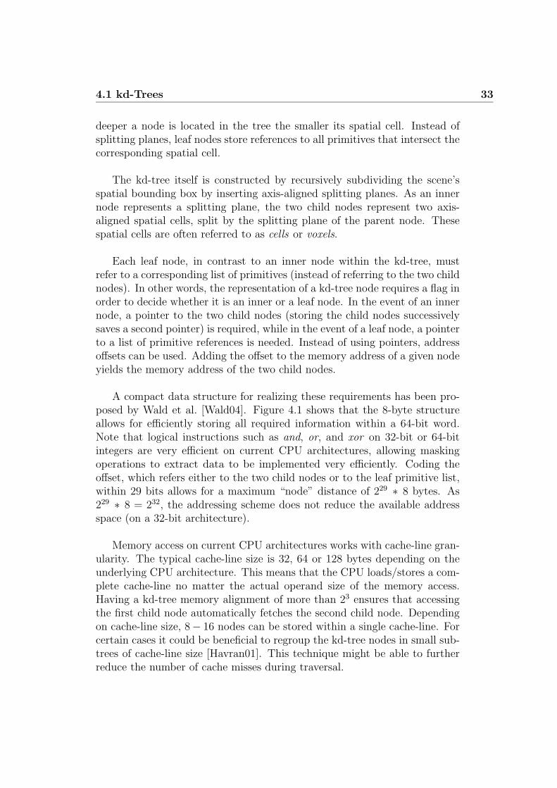
4.1 kd-Trees 33
deeper a node is located in the tree the smaller its spatial cell. Instead ofsplitting planes, leaf nodes store references to all primitives that intersect thecorresponding spatial cell.
The kd-tree itself is constructed by recursively subdividing the scene’sspatial bounding box by inserting axis-aligned splitting planes. As an innernode represents a splitting plane, the two child nodes represent two axis-aligned spatial cells, split by the splitting plane of the parent node. Thesespatial cells are often referred to as cells or voxels.
Each leaf node, in contrast to an inner node within the kd-tree, mustrefer to a corresponding list of primitives (instead of referring to the two childnodes). In other words, the representation of a kd-tree node requires a flag inorder to decide whether it is an inner or a leaf node. In the event of an innernode, a pointer to the two child nodes (storing the child nodes successivelysaves a second pointer) is required, while in the event of a leaf node, a pointerto a list of primitive references is needed. Instead of using pointers, addressoffsets can be used. Adding the offset to the memory address of a given nodeyields the memory address of the two child nodes.
A compact data structure for realizing these requirements has been pro-posed by Wald et al. [Wald04]. Figure 4.1 shows that the 8-byte structureallows for efficiently storing all required information within a 64-bit word.Note that logical instructions such as and, or, and xor on 32-bit or 64-bitintegers are very efficient on current CPU architectures, allowing maskingoperations to extract data to be implemented very efficiently. Coding theoffset, which refers either to the two child nodes or to the leaf primitive list,within 29 bits allows for a maximum “node” distance of 229 ∗ 8 bytes. As229 ∗ 8 = 232, the addressing scheme does not reduce the available addressspace (on a 32-bit architecture).
Memory access on current CPU architectures works with cache-line gran-ularity. The typical cache-line size is 32, 64 or 128 bytes depending on theunderlying CPU architecture. This means that the CPU loads/stores a com-plete cache-line no matter the actual operand size of the memory access.Having a kd-tree memory alignment of more than 23 ensures that accessingthe first child node automatically fetches the second child node. Dependingon cache-line size, 8− 16 nodes can be stored within a single cache-line. Forcertain cases it could be beneficial to regroup the kd-tree nodes in small sub-trees of cache-line size [Havran01]. This technique might be able to furtherreduce the number of cache misses during traversal.

34 Chapter 4: Tracing Coherent Ray Bundles
// efficient 8-byte layout for a kd-tree node
struct KDTreeNode {
union
{
float split_position; // position of axis-aligned split plane
unsigned int items; // or number of leaf primitives
}
unsigned int dim_offset_flag;
// the 32 bits of ’dim_offset_flag’ are used to encode multiple data
// bits[0..1] : encode the split plane dimension
// bits[2..30] : encode an address offset
// bit[31] : encodes whether a node is an inner node or a leaf
};
// macros for extracting node information
#define ISLEAF(n) (n->dim_offset_flag & (unsigned int)(1<<31))
#define DIMENSION(n) (n->dim_offset_flag & 0x3)
#define OFFSET(n) (n->dim_offset_flag & 0x7FFFFFFC)
Figure 4.1: kd-tree node layout using only eight bytes. In combination witha proper memory alignment of more than 23 bytes, the kd-tree node layoutallows for storing the split dimension within the two lowest bits. The highestbit decides between inner and leaf node, while the remaining 29 bits encodean address offset (substituting a pointer) to either the child nodes or to anindex list of primitives.
4.2 Ray Bundle Traversal I
Fast traversal through a kd-tree is essential for achieving high ray tracingperformance because the operation is the one most frequently performed.In order to provide a better understanding of the traversal algorithm forbundles, a brief review of the algorithm for single rays is given first.
4.2.1 The Ray-Segment Algorithm for Single Rays
The traversal algorithm basically consists of the following operations: De-scend from the kd-tree root node in a front-to-back manner (required byearly ray termination) by either following the front, the back, or both chil-dren until a leaf is reached. In the case of following both children, continuewith the front child and push the kd-tree node referring to the back child ontoa stack. If a leaf is reached, test all entries in the leaf’s primitive referencelist (typically, indices referring to a list of scene primitives) for intersection.
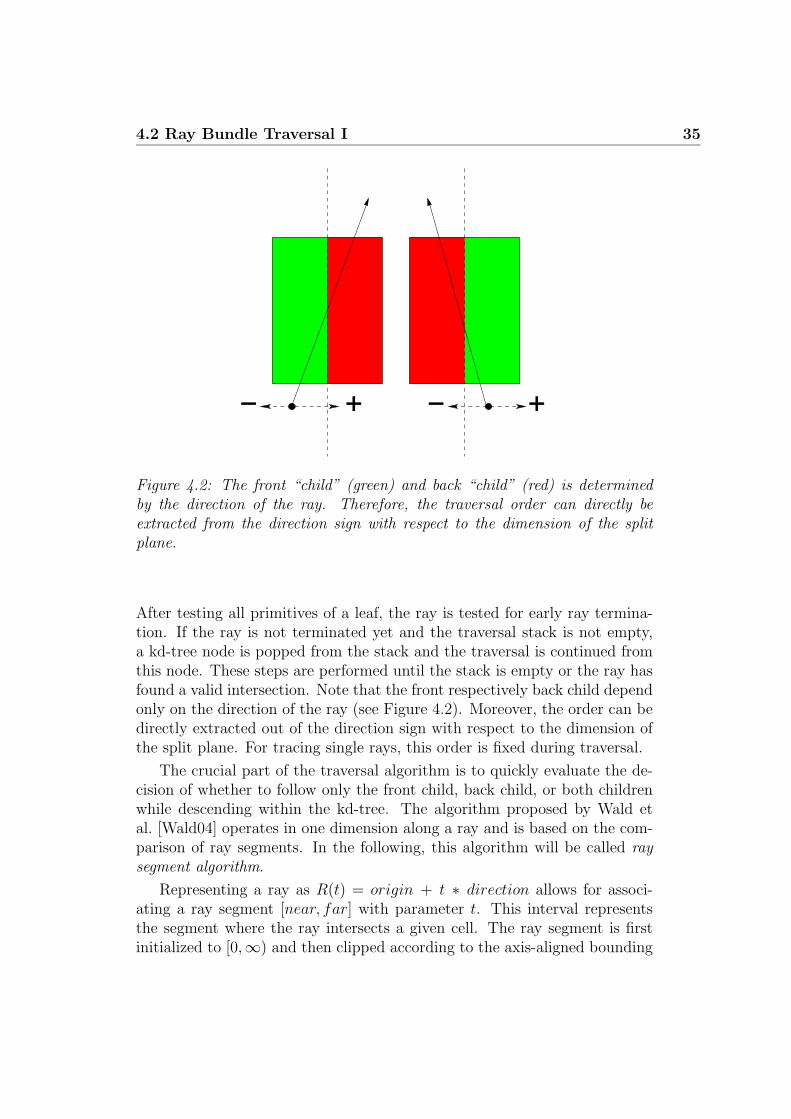
4.2 Ray Bundle Traversal I 35
++ −−
Figure 4.2: The front “child” (green) and back “child” (red) is determinedby the direction of the ray. Therefore, the traversal order can directly beextracted from the direction sign with respect to the dimension of the splitplane.
After testing all primitives of a leaf, the ray is tested for early ray termina-tion. If the ray is not terminated yet and the traversal stack is not empty,a kd-tree node is popped from the stack and the traversal is continued fromthis node. These steps are performed until the stack is empty or the ray hasfound a valid intersection. Note that the front respectively back child dependonly on the direction of the ray (see Figure 4.2). Moreover, the order can bedirectly extracted out of the direction sign with respect to the dimension ofthe split plane. For tracing single rays, this order is fixed during traversal.
The crucial part of the traversal algorithm is to quickly evaluate the de-cision of whether to follow only the front child, back child, or both childrenwhile descending within the kd-tree. The algorithm proposed by Wald etal. [Wald04] operates in one dimension along a ray and is based on the com-parison of ray segments. In the following, this algorithm will be called raysegment algorithm.
Representing a ray as R(t) = origin + t ∗ direction allows for associ-ating a ray segment [near, far] with parameter t. This interval representsthe segment where the ray intersects a given cell. The ray segment is firstinitialized to [0,∞) and then clipped according to the axis-aligned bounding
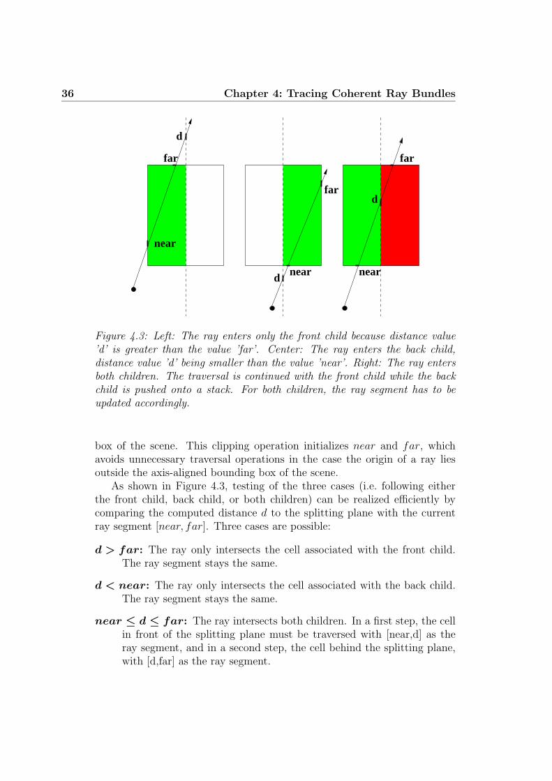
36 Chapter 4: Tracing Coherent Ray Bundles
far
near
far
d
d near
far
d
near
Figure 4.3: Left: The ray enters only the front child because distance value’d’ is greater than the value ’far’. Center: The ray enters the back child,distance value ’d’ being smaller than the value ’near’. Right: The ray entersboth children. The traversal is continued with the front child while the backchild is pushed onto a stack. For both children, the ray segment has to beupdated accordingly.
box of the scene. This clipping operation initializes near and far, whichavoids unnecessary traversal operations in the case the origin of a ray liesoutside the axis-aligned bounding box of the scene.
As shown in Figure 4.3, testing of the three cases (i.e. following eitherthe front child, back child, or both children) can be realized efficiently bycomparing the computed distance d to the splitting plane with the currentray segment [near, far]. Three cases are possible:
d > far: The ray only intersects the cell associated with the front child.The ray segment stays the same.
d < near: The ray only intersects the cell associated with the back child.The ray segment stays the same.
near ≤ d ≤ far: The ray intersects both children. In a first step, the cellin front of the splitting plane must be traversed with [near,d] as theray segment, and in a second step, the cell behind the splitting plane,with [d,far] as the ray segment.

4.2 Ray Bundle Traversal I 37
d
d
far
far
dnear
far
d
0d
1
0d
1
1
1
d0
near
0d
1
nearnear
far0
far1
1
0near
0
1near0
near1
far
10
far0
near0 1
1
0far
Figure 4.4: For all ray bundles a common origin is assumed. Left: All raysenter the cell of the front child as all distance values ’di’ are greater thanthe values ’fari’. Center left: All rays enter the cell of the back child as alldistance values ’di’ are lower than the values ’neari’. Center right: If only asingle ray traverses both children, all rays have to follow. Right: The cells ofthe front and the back child have to be accessed again, but the ray bundle hasdifferent direction signs. Even in this case, a common front-back decision ispossible: All rays first access the cell of the child containing the origin.
One advantage of the ray segment algorithm is that it requires only ashort sequence of simple instructions. In particular, only the parametricdistance d has to be computed, followed by the two comparisons with thenear and far value. Based on these comparisons, one of the three cases hasto be determined and the traversal is continued accordingly.
4.2.2 The Ray-Segment Algorithm for Ray Bundles
Traversal for bundles of rays relies on the same idea of comparing ray seg-ments as shown for single rays (see Section 4.2.1). Instead of a single interval[near, far], n intervals [neari, fari], where n is the number of rays within thebundle, have to be used. Note that in the following it is assumed that all rayswithin a bundle have a common origin, while the case of arbitrary originswill be discussed later on. This assumption allows for a common traversalorder in the event of varying ray direction signs.

38 Chapter 4: Tracing Coherent Ray Bundles
Figure 4.4 illustrates that if the segment comparison for all rays is iden-tical (di > fari or di < neari), only one child has to be traversed similarlyto the single ray case. In all other cases, both children must be traversed.In other words: If any ray indicates a specific child, all rays have to follow.This illustrates why coherence within the ray bundle is essential for achievinghigh performance, because the more coherent the rays are the more likely itis that all rays make the same decision.
Attention must be given to determining the front and back order whenboth children have to be traversed. In the case that all rays have the samedirection sign (with respect to the split dimension), the front and back childis unambiguously determined (as in the single ray case). If the ray directionsigns vary but (as assumed) all rays have a common origin, a non-ambiguousorder (see Figure 4.4) is still ensured, because all rays first traverse the childcontaining the origin.
Computing the appropriate order every time from scratch during traversalcan be quite complex. Therefore, it can be beneficial to split the rays intobundles with equal direction signs before the traversal. Moreover, in practiceonly a few bundles need to be split up. For more simplicity, the case of equaldirection signs is assumed for all subsequent code examples.
A similar procedure can be applied if the rays within the bundle do notshare a common origin and ray directions differ. In this case, no consistentfront and back order can be determined. The best way to ensure a consistentorder is to split the rays into bundles containing only rays with equal raydirections ensuring a common traversal decision.
4.2.3 Implementation
In the following, an example implementation for the ray segment traversalalgorithm for ray bundles is proposed. The implementation is optimized forexploiting SIMD features by using SSE intrinsics. As SSE operates on fourfloating point values at once, it is beneficial to use ray bundles with a multipleof four rays. The implementation is divided into three parts: Initialization,traversal order determination, and the traversal operation itself.
Initialization
The initial clipping against the scene bounding box computes the minimumand the maximum parametric distances to all three plane slabs [Kay86] (abox is defined as the intersection of three slabs). Figure 4.5 shows the SSEimplementation for a bundle of four rays. Note that values of clip min andclip max will be exchanged according to the ray directions, before updating

4.2 Ray Bundle Traversal I 39
near4 and far4. During traversal, the parametric distance d to the splittingplane is computed as d = (split − origin) ∗ 1/direction. By precomputing1/direction a costly division operation is avoided. Note that the inversecomputation does not have to be performed at this point, e.g. the inverse ofdirections for primary rays can be initialized when the rays are generated.
sse_t near4 = _mm_setzero_ps(); // -- four ray segments --
sse_t far4 = _mm_set_ps1(Infinity);
SSEVec4 oneOverDirection; // -- 1.0 / ray4.direction --
// -- clipping in the x dimension --
oneOverDirection4.t[0] = Inverse4(ray4.direction.t[0]);
// compute minimum distance by (box.min.x - origin.x) * 1.0/direction.x
const sse_t clip_min = _mm_mul_ps(_mm_sub_ps(_mm_set_ps1(box.min.x),
ray4.origin.t[0]),
oneOverDirection.t[0]);
// compute maximum distance by (box.max.x - origin.x) * 1.0/direction.x
const sse_t clip_max = _mm_mul_ps(_mm_sub_ps(_mm_set_ps1(box.max.x),
ray4.origin.t[0]),
oneOverDirection4.t[0]);
// update near4 and far4 based on the minimum and maximum distance
const sse_t cmp = _mm_cmpgt_ps(ray4.direction.t[0],_mm_setzero_ps());
near4 = _mm_max_ps(near4,Update4(cmp,clip_min,clip_max));
far4 = _mm_min_ps( far4,Update4(cmp,clip_max,clip_min));
Figure 4.5: Initial segment initialization for a four-ray bundle. The four raysegments are stored within the two SSE variables ’near4’ and ’far4’. After ini-tialization, one clipping step against the scene bounding box, here in the firstdimension, is applied. Clipping in the other two dimensions is implementedaccordingly. The inverse of the directions is stored in the ’oneOverDirection4’structure.
In order to achieve a common traversal order, it is necessary to split up aray bundle with different ray directions into bundles with equal ray directions.This case can be quickly detected by comparing the direction signs of allrays within the bundle. The signs for a four-ray bundle can be extracted bya simple mm movemask ps instruction. This instruction extracts the signbits of all register elements, and stores the final 4-bit result within a generalpurpose register. In the case the four signs are equal (either 0 or 0xf) withrespect to all three dimensions, the bundle does not need to be split. The
40 Chapter 4: Tracing Coherent Ray Bundles
splitting operation can actually be seen as a sorting of ray directions into theeight coordinate system octants. Each octant ensures equal ray directions,and can therefore be processed without further splitting.
In the case a ray does not enter the scene bounding box it should notinfluence any decision in the traversal and intersection. Therefore, such in-valid rays have to be identified and deactivated. Fortunately, the clippingstep automatically sets the ray segment for invalid rays to the invalid state ofnear > far. Detecting this case by performing an SSE comparison betweennear4 and far4 allows for using the bit-mask result as a valid/invalid maskfor rays.
const unsigned int dir_x = *(unsigned int *)(&ray4.direction.t[0]);
const unsigned int dir_y = *(unsigned int *)(&ray4.direction.t[1]);
const unsigned int dir_z = *(unsigned int *)(&ray4.direction.t[2]);
const unsigned int ray_dir_x = (dir_x & ((unsigned int)1<<31))) >> 28;
const unsigned int ray_dir_y = (dir_y & ((unsigned int)1<<31))) >> 28;
const unsigned int ray_dir_z = (dir_z & ((unsigned int)1<<31))) >> 28;
const unsigned int ray_dir[3][2] = {
{ ray_dir_x,ray_dir_x^((unsigned int)1 << 3) },
{ ray_dir_y,ray_dir_y^((unsigned int)1 << 3) },
{ ray_dir_z,ray_dir_z^((unsigned int)1 << 3) } };
Figure 4.6: Precomputing the traversal order (front and back child) as offsetsfor a bundle of rays with equal directions. For a given dimension ’d’, thefront child has an offset of ’ray dir[d][0]’, and the back child of ’ray dir[d][1]’.In order to efficiently obtain the pointer to the front respectively back childof the current kd-tree node, only the precomputed offset has to be added tothe current node address. Note that the size of a kd-tree node is 8 bytes.Therefore, the extracted sign bit must be right-shifted by 28 bits. The offsettable contains only the values 8 or 0.
Traversal Order
Under the condition of a common traversal order, it is only necessary todecide which of the left or right kd-tree child node is the front respectivelyback child. By using a small array of two integer offsets per dimension, asshown in Figure 4.6, the offset to the front and back child can be precomputed(based on the direction signs) for the whole bundle. As all rays within thebundle have equal directions signs, the simplification can be made to initializethe offset table with the data of the first ray of the bundle.
The offset table itself allows for speeding up the inner-traversal loop be-cause it avoids recomputing the offset for every traversal step. Computing
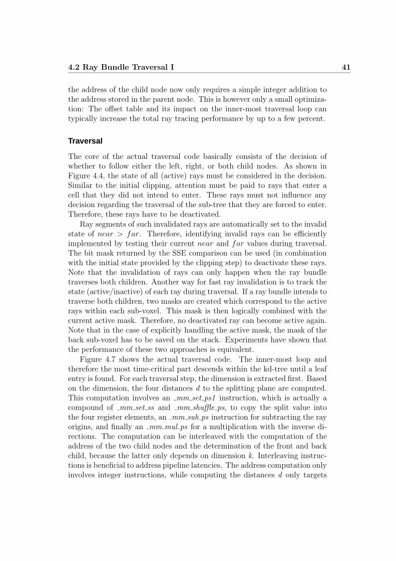
4.2 Ray Bundle Traversal I 41
the address of the child node now only requires a simple integer addition tothe address stored in the parent node. This is however only a small optimiza-tion: The offset table and its impact on the inner-most traversal loop cantypically increase the total ray tracing performance by up to a few percent.
Traversal
The core of the actual traversal code basically consists of the decision ofwhether to follow either the left, right, or both child nodes. As shown inFigure 4.4, the state of all (active) rays must be considered in the decision.Similar to the initial clipping, attention must be paid to rays that enter acell that they did not intend to enter. These rays must not influence anydecision regarding the traversal of the sub-tree that they are forced to enter.Therefore, these rays have to be deactivated.
Ray segments of such invalidated rays are automatically set to the invalidstate of near > far. Therefore, identifying invalid rays can be efficientlyimplemented by testing their current near and far values during traversal.The bit mask returned by the SSE comparison can be used (in combinationwith the initial state provided by the clipping step) to deactivate these rays.Note that the invalidation of rays can only happen when the ray bundletraverses both children. Another way for fast ray invalidation is to track thestate (active/inactive) of each ray during traversal. If a ray bundle intends totraverse both children, two masks are created which correspond to the activerays within each sub-voxel. This mask is then logically combined with thecurrent active mask. Therefore, no deactivated ray can become active again.Note that in the case of explicitly handling the active mask, the mask of theback sub-voxel has to be saved on the stack. Experiments have shown thatthe performance of these two approaches is equivalent.
Figure 4.7 shows the actual traversal code. The inner-most loop andtherefore the most time-critical part descends within the kd-tree until a leafentry is found. For each traversal step, the dimension is extracted first. Basedon the dimension, the four distances d to the splitting plane are computed.This computation involves an mm set ps1 instruction, which is actually acompound of mm set ss and mm shuffle ps, to copy the split value intothe four register elements, an mm sub ps instruction for subtracting the rayorigins, and finally an mm mul ps for a multiplication with the inverse di-rections. The computation can be interleaved with the computation of theaddress of the two child nodes and the determination of the front and backchild, because the latter only depends on dimension k. Interleaving instruc-tions is beneficial to address pipeline latencies. The address computation onlyinvolves integer instructions, while computing the distances d only targets

42 Chapter 4: Tracing Coherent Ray Bundles
unsigned int activeMask = 0xf, termination = 0, index = 0;
union { KDTreeNode *node; unsigned int adr; };
node = scene->root; // root of kd-tree
do { // traverse until a leaf is reached
while (!ISLEAF(node)) {
const unsigned int k = DIMENSION(node);
const sse_t d = _mm_mul_ps(_mm_sub_ps(_mm_set_ps1(node->split),
ray4.origin.t[k]),
oneOverDirection4.t[k]);
adr += OFFSET(node);
KDTreeNode *back = (KDTreeNode *)(adr + ray_dir[k][1]);
KDTreeNode *front = (KDTreeNode *)(adr + ray_dir[k][0]);
node = back; // only back child traversal ?
if (!(_mm_movemask_ps(_mm_cmple_ps(near4,d)) & activeMask)) continue;
node = front; // only front child traversal ?
if (!(_mm_movemask_ps(_mm_cmpge_ps(far4,d)) & activeMask)) continue;
stackNode[index] = back; // push values on stack
stackSSE4[index].near4 = _mm_max_ps(near4,d);
stackSSE4[index].far4 = far4;
index++;
far4 = _mm_min_ps(far4,d); // update far values and the active mask
activeMask &= _mm_movemask_ps(_mm_cmple_ps(near4,far4));
}
if (node->items) {
// ... intersection code ...
termination |= activeMask &
_mm_movemask_ps(_mm_cmpge_ps(far4,hit4.dist));
if (termination == 0xf) return; // valid intersections -> terminate
}
if ( index == 0 ) return; // stack empty -> terminate
index--; // pop values from the stack and update active mask
node = stackNode[index];
near4 = stackSSE4[index].near4;
far4 = stackSSE4[index].far4;
activeMask = ~termination & _mm_movemask_ps(_mm_cmple_ps(near4,far4));
} while(1);
Figure 4.7: SSE traversal code for a bundle of four rays (with equal directionsigns). The four lowest bits of ’activeMask’ correspond to the current raystate (activated/deactivated), which is based on the current relation between’near4’ and ’far4’. The code consists of three parts: Traversal until a leafis reached, then perform (possible) primitive intersection tests, and if notall rays are set for early ray termination, starting a new traversal iterationwith values taken from the stack. When taking an entry from the stack the’activeMask’ is updated with the mask of the already terminated rays.

4.2 Ray Bundle Traversal I 43
the floating point pipeline. The out-of-order execution unit of the processoris able to execute these instructions mostly in parallel.
The decision whether to traverse the front child, back child, or bothchildren is computed by only considering active rays. The lowest four bitsof activeMask indicate the current state of all four rays. Applying a logicaland between activeMask and the result of SSE comparison between d andnear4 respectively far4, automatically sets the flag register, removing theneed for an additional compare instruction. The first comparison between dand near4 tests if no ray requires to access the front child. If this conditionis true all rays will go to the back child. The second comparison for testingthe front child (no ray needs to access the back child) based on d and far4,works accordingly.
If both the front and the back children have to be considered, the activemask is updated based on the current values by applying a logical and be-tween near4 and far4. This is done because a deactivated ray can neverbecome active again, so the number of active rays will only become smallerwhile descending the tree. Additionally, the back node and the correspond-ing far value are pushed onto the stack, and the corresponding stack indexis increased.
The two branches within the inner-most traversal loop are only taken ifall rays go either exclusively to the front or back child. These two casesshould be arranged before the case of traversing both children, because themore coherent the rays are the lower the probability for the later case. Theprobability of the front and back branch depends on the scene and in par-ticular on the view, which is why the branch arrangement does not mattersignificantly. Statistics have shown that for coherent rays all three cases oc-cur with equal probability. Therefore, the two exclusive branches are takenwith an average probability of 2/3 and require fewer instructions than theboth child case.
In terms of cache misses, the critical memory access occurs when loadingthe data of a kd-tree node from memory. Reducing the cache misses byinserting prefetch instructions fails because the traversal code is too small tocompletely hide the memory latency. On current CPU architectures, roughly200 cycles are required to hide the latency of main memory accesses. On theother hand, the CPU cache hierarchy ensures a reasonable cache hit ratebecause of the locality of kd-tree node accesses.
When reaching a leaf node an empty test is applied first. As advancedkd-tree construction tends to cut off empty space as much as possible, manyempty leaves will be created. In the case that the current leaves is not empty,intersection tests, e.g. for triangles (see Chapter 5) are performed based ona primitive index list.

44 Chapter 4: Tracing Coherent Ray Bundles
After performing all intersection tests, all rays are checked for early raytermination. Note that only those rays are marked as terminated whoseintersection distance is smaller than the current far value and the corre-sponding active masks are set. If the distance is higher than the current farvalue, a potential new intersection could exist between the current far andthe intersection distance.
At the end, if the stack is not empty, the corresponding values are takenfrom the stack and traversal is restarted. Before restarting traversal, theactive mask is reset based on the updated near and far values, and on anynewly terminated rays.
The code in Figure 4.7 stores the active mask as an integer bit mask.On some CPU architectures, it is more beneficial to hold the active withinSSE registers, and apply an mm and ps before transferring the result of thecomparison using the mm movemask ps instruction. The latter also suffersfrom a very high latency of 7 or more cycles (on current architectures). Thehigh latency results from the fact that the asynchronously running integerand floating point pipelines have to be synchronized.
Further critical performance hot spots are the two branches because theyare purely data dependent. Therefore, the processor’s branch prediction unitcannot really reduce the amount of mis-predicted branches. Besides the im-pact of branch mis-prediction, the traversal code for four rays has a lot of datadependencies, making parallel out-of-order execution difficult. For largerbundles, some operations like the computation of the split plane distancescan be done in parallel across all four-ray bundles. Nevertheless, branchingaccording to the three traversal cases requires the comparison results of allfour-ray bundles. This introduces implicit synchronization, limiting the coderegions for potential parallel execution.
Extension: Removing Branches
The traversal loop can be implemented without branches (see Figure 4.8)because a mis-predicted branch causes a pipeline stall up to the length of theprocessor’s execution pipeline.
Current CPU architectures allow for using conditional move instructionsto prevent branching. These instructions move a value to a register only ifa specific condition holds true. Current C/C++ compilers [Intel02a, GNU]tend to use such conditional move instructions through the ?: operator, ifboth operands are constant values. The code shown in Figure 4.8 applies thisoperator for setting the traversal side. Note that the conditional ?: operatorrepresents only a hint for the compiler to use a conditional move instruction,not a must. Depending on the compiler, it is helpful to manually modify
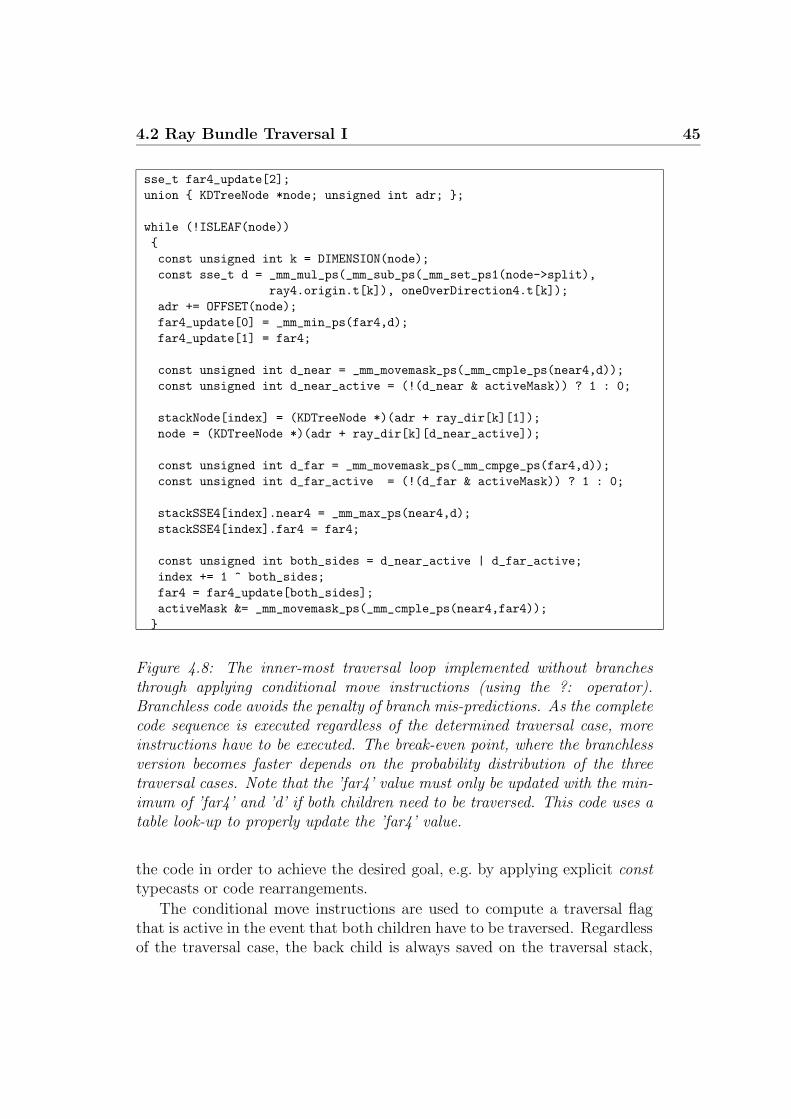
4.2 Ray Bundle Traversal I 45
sse_t far4_update[2];
union { KDTreeNode *node; unsigned int adr; };
while (!ISLEAF(node))
{
const unsigned int k = DIMENSION(node);
const sse_t d = _mm_mul_ps(_mm_sub_ps(_mm_set_ps1(node->split),
ray4.origin.t[k]), oneOverDirection4.t[k]);
adr += OFFSET(node);
far4_update[0] = _mm_min_ps(far4,d);
far4_update[1] = far4;
const unsigned int d_near = _mm_movemask_ps(_mm_cmple_ps(near4,d));
const unsigned int d_near_active = (!(d_near & activeMask)) ? 1 : 0;
stackNode[index] = (KDTreeNode *)(adr + ray_dir[k][1]);
node = (KDTreeNode *)(adr + ray_dir[k][d_near_active]);
const unsigned int d_far = _mm_movemask_ps(_mm_cmpge_ps(far4,d));
const unsigned int d_far_active = (!(d_far & activeMask)) ? 1 : 0;
stackSSE4[index].near4 = _mm_max_ps(near4,d);
stackSSE4[index].far4 = far4;
const unsigned int both_sides = d_near_active | d_far_active;
index += 1 ^ both_sides;
far4 = far4_update[both_sides];
activeMask &= _mm_movemask_ps(_mm_cmple_ps(near4,far4));
}
Figure 4.8: The inner-most traversal loop implemented without branchesthrough applying conditional move instructions (using the ?: operator).Branchless code avoids the penalty of branch mis-predictions. As the completecode sequence is executed regardless of the determined traversal case, moreinstructions have to be executed. The break-even point, where the branchlessversion becomes faster depends on the probability distribution of the threetraversal cases. Note that the ’far4’ value must only be updated with the min-imum of ’far4’ and ’d’ if both children need to be traversed. This code uses atable look-up to properly update the ’far4’ value.
the code in order to achieve the desired goal, e.g. by applying explicit consttypecasts or code rearrangements.
The conditional move instructions are used to compute a traversal flagthat is active in the event that both children have to be traversed. Regardlessof the traversal case, the back child is always saved on the traversal stack,

46 Chapter 4: Tracing Coherent Ray Bundles
#define FOR_ALL_BUNDLES for (unsigned int i=0;i<BUNDLES;i++)
while (!ISLEAF(node))
{
const sse_t node_split = _mm_set_ps1(node->split);
const unsigned int k = DIMENSION(node);
adr += OFFSET(node);
KDTreeNode *front = (KDTreeNode *)(adr + ray_dir[k][0]);
KDTreeNode *back = (KDTreeNode *)(adr + ray_dir[k][1]);
unsigned int d_near = 0, d_far = 0;
sse_t d[BUNDLES];
FOR_ALL_BUNDLES
{
d[i] = _mm_mul_ps(_mm_sub_ps(node_split,ray4[i].origin.t[k]),
oneOverDirection4[i].t[k]);
d_near |= _mm_movemask_ps(_mm_and_ps(_mm_cmple_ps(near4[i],d[i]),
activeMask[i]));
d_far |= _mm_movemask_ps(_mm_and_ps(_mm_cmpge_ps(far4[i],d[i]),
activeMask[i]));
};
node = back;
if (d_near == 0) { continue; } // traverse the back child
node = front;
if (d_far == 0) { continue; } // traverse the front child
// traverse both children => push values on the stack
FOR_ALL_BUNDLES {
stackISSE[stackIndex].far4[i] = far4[i];
stackISSE[stackIndex].near4[i] = _mm_max_ps(near4[i],d[i]);
far4[i] = _mm_min_ps(far4[i],d[i]);
activeMask[i] = _mm_and_ps(activeMask[i],
_mm_cmple_ps(near4[i],far4[i]));
}
stackNode[stackIndex] = back;
stackIndex++;
}
Figure 4.9: The inner-most traversal loop for an arbitrary number of four-ray bundles. The implementation relies on the same algorithm as shown inFigure 4.7. Note that for each four-ray bundle, the ’activeMask’ is stored asSSE data type.
but the stack pointer is only updated if the traversal flag is active. A similarmechanism is applied for updating the far4 value: Both the original and amodified far4 value are stored into a table, and the far4 is set by a tablelook-up based on the traversal flag. Updating the far4 could be implementedby a sequence of conditional move instructions, but a table look-up is usuallyfaster.
4.2 Ray Bundle Traversal I 47
As the branchless version executes more instructions as the version withbranches, the break-even point where the branchless version becomes fasterdepends on the probability distribution of the three traversal cases. Themore likely the both-side case is, the more beneficial the branchless versionwill be. Therefore, ray bundles with a low coherence are more suitable forthe branchless version.
Extension: Tracing Multiple Ray Bundles
Extending the code to trace more than four rays in parallel is straightforward.As SSE operates on four elements, it is beneficial to handle multiples of four-ray bundles, e.g. four four-ray bundles corresponding to 16 rays. Note that16 rays require four near4 and four far4 values. Unfortunately, the eightSSE registers (on standard 32-bit Intel or AMD architectures) do not allowfor holding all near4 and far4 values within registers during traversal. Thisintroduces additional memory accesses (temporary values must be stored tomemory). An alternative implementation could store the activeMask as aninteger value, instead of using the sse t data type. Which way is actuallyfaster, largely depends on the actual architecture used.
Figure 4.9 shows the traversal loop for an arbitrary number of four-raybundles. Note that computing distances di, and the corresponding com-parisons to neari and fari for a bundle i is independent of other bundles,allowing for an increased instruction level parallelism.
Moreover, the decision to follow only one side comes up roughly in themiddle of the traversal code. This means, the more likely the one-side casehappens the more often half of the traversal code is skipped. One couldeasily implement the traversal code for multiple bundles without branches,following the same approach as shown in Figure 4.8. Whether this approachis beneficial or not, largely depends on the probability that both childrenmust be traversed as well as the penalty cost for a mis-predicted branch.
Extension: Tracing Multiple Ray Bundles With Masking
Apart from the given code examples, many implementation variants are pos-sible. As mentioned in the beginning of this section, storing the active maskas integer directly on the stack will avoid updating the active mask basedon the current near and far values. Moreover, the complete front/back childdetermination can be recoded in a left/right child decision using a sequenceof Boolean expressions (see Figure 4.10).
As the fact that the front or back child only depends on the ray directions,they can be evaluated on the fly. Therefore, all ray directions (with respect to

48 Chapter 4: Tracing Coherent Ray Bundles
#define FOR_ALL_BUNDLES for (unsigned int i=0;i<BUNDLES;i++)
unsigned int activeMask = 0xffff;
while (!ISLEAF(node)) {
const sse_t node_split = _mm_set_ps1(node->split);
const unsigned int k = DIMENSION(node);
adr += OFFSET(node);
unsigned int dgef = 0; unsigned int dlen = 0;
sse_t d[BUNDLES];
FOR_ALL_BUNDLES {
d[i] = _mm_mul_ps(_mm_sub_ps(node_split,ray4[i].origin.t[k]),
oneOverDirection4[i].t[k]);
dlen |= _mm_movemask_ps(_mm_cmpgt_ps(near4[i],d[i])) << (4*i);
dgef |= _mm_movemask_ps(_mm_cmpgt_ps(d[i],far4[i])) << (4*i);
};
const unsigned int bactive = ((dgef^0xffff) &
(dlen^0xffff)) & activeMask;
dgef &= activeMask; dlen &= activeMask;
// active rays that require to traverse the right child
const unsigned int ractive = (dgef & dir[k]) |
(dlen & (dir[k]^0xffff)) | bactive;
// active rays that require to traverse the left child
const unsigned int lactive = (dgef & (dir[k]^0xffff)) |
(dlen & dir[k]) | bactive;
if (lactive == 0) { adr += 8; continue; } // traverse the right child
if (ractive == 0) { adr += 0; continue; } // traverse the left child
FOR_ALL_BUNDLES {
stackISSE[stackIndex].far4[i] = far4[i];
stackISSE[stackIndex].near4[i] = _mm_max_ps(near4[i],d[i]);
far4[i] = _mm_min_ps(far4[i],d[i]);
}
const unsigned int side = (bactive & dir[k]) != 0;
node += side;
stackNode[stackIndex] = (KDTreeNode*)adr^8;
stackNode[stackIndex] = side ? lactive : ractive;
activeMask &= side ? ractive : lactive;
stackIndex++;
}
Figure 4.10: The inner-most traversal loop for up to eight four-ray bundles(all rays must have the same direction sign). Instead of holding the ray activemask within multiple SSE registers, the mask is stored as a bit mask withina single integer register (requiring more ’ mm movemask ps’ instructions).The decision of whether to follow the front or back child is modified into adecision of whether to follow the left child (offset 0) or the right child (offset8).

4.3 Ray Bundle Traversal II 49
the three dimensions) are extracted and stored as bit-masks into three integervariables. Depending on the split dimension, one of these three directionmasks is applied to determine the front and back child, respectively.
Compared to the code example of Figure 4.9, the deactivation of invalidrays is not performed by SSE instructions but integer instructions. Depend-ing on the architectures, this modification can be beneficial but in generalthe two implementations provide similar performance.
Future Modifications
If a future version of the SSE instruction set includes a multiply-add in-struction, the dependency chain for computing the distances to the splittingplane can be reduced. Instead of performing (split − origin) ∗ 1/direction,one could rearrange this code sequence to split ∗ 1/direction − origin ∗1/direction, while the −origin ∗ 1/direction could be precomputed. Therearrangement allows for directly applying a multiply-add instruction of theform a ∗ b + c.
Note that there is no unique fastest code sequence. Depending on thearchitecture, in particular on the throughput and latency of the instructions,one has to choose an appropriate implementation. Moreover, some optimiza-tion techniques are beneficial for a certain architecture, e.g. the Pentium-IV,but are disadvantageous for other architectures such as the Opteron.
4.3 Ray Bundle Traversal II
Reshetov et al. [Reshetov05] proposed an alternative traversal algorithmwhich does not consider the decision of each ray in order to determine thebehavior of the whole bundle. Instead, the algorithm efficiently culls partsof a kd-tree which are known not to be intersected by the frustum spawnedby the rays within the bundle. The underlying culling technique is calledinverse frustum culling.
4.3.1 The Inverse Frustum Culling Algorithm
Inverse frustum culling allows for efficiently culling the axis-aligned boundingboxes (AABBs) associated with kd-tree cells by using the faces of a givenAABB as separation planes. If one of these planes separates the ray bundlefrom the AABB, the corresponding cell can be efficiently culled.
Figure 4.11 illustrates the approach by using a 2D example. A given cellassociated to a kd-tree node is split into two sub-cells (associated to the two

50 Chapter 4: Tracing Coherent Ray Bundles
dmin dmax s min s max dmaxdmins min s maxS S
Figure 4.11: Traversal for ray bundles by comparing only extremal values: Ifthe extremal intersection value ’dmax’ (’dmin’) of all intersections with split-ting plane ’S’ is less (greater) than ’smin’ (’smax’) (the bounds of ’S’ withrespect to the current cell), only the front (back) cell, colored green (white),has to be considered further, while the back (front) is completely culled. Thenon-culled cell is marked green. If none of the two cases is valid, both cellshave to be considered. Note that the culling test has to be applied in twodimensions, i.e. given split dimension ’x’, the two culling tests have to beapplied to the other two dimension ’y’ and ’z’.
child nodes) by split plane S. In a first step, the algorithm computes the in-tersection values di for all rays within the bundle with splitting plane S. Onthe assumption that the bundle intersects the given cell, the intersected sub-cell(s) has/have to be determined. Determining the sub-cell can be efficientlyrealized by only comparing the extremal values of all ray-splitting-plane in-tersections di with the bounded interval [smin, smax] of splitting plane S.
Knowing the extremal values of ray directions in advance allows for han-dling large bundles of rays without considering all rays during traversal. As-suming a standard perspective camera for generating primary rays, these ex-tremal values correspond to the corner rays of a small N×N pixel block. Thedefinition of all rays within the bundle must only be known when entering anon-empty leaf, especially for performing the ray-primitive intersection tests.

4.3 Ray Bundle Traversal II 51
Depending on the common direction of rays within the bundle, only twocases have to be considered:
dmax < smin: All intersection points di are lower than smin. All rays willonly intersect the cell associated to the front child.
dmin > smax: All intersection points di are greater than smax. All rays willonly intersect the cell associated to the back child.
In all other cases both children have to be traversed.Applying the algorithm to 3D requires the comparison to be made in
two dimensions: For example, given a split plane parallel to the yz-planethe intervals in y and z direction have to be used. Furthermore, not onlythe front and back child but also the roles of dmin and dmax depend on thecommon ray directions within the bundle.
4.3.2 Implementation
In contrast to the algorithm in Section 4.2, the traversal does not rely onhandling ray segments but on continuously updating the axis-aligned bound-ing box referring to the current kd-tree voxel. Representing the axis-alignedbounding box by the two extremal points, as shown in Figure 3.10, allowsfor efficiently updating the current box. The extremal component of the boxwhich has to be updated depends on the common ray directions.
Initialization
As pointed out, certain parts of the algorithm depend on the common ray di-rections. The eight possible cases, corresponding to the eight octants, couldbe implemented separately. The appropriate case only needs to be deter-mined once and in particular before the actual traversal starts. In the fol-lowing, a different implementation is used. The determination of the traver-sal case is done in the inner-most traversal code but using data-dependentreads. Therefore, using look-up tables, e.g. for storing integer offsets to ex-tremal points with the box structure (see Figure 4.12) allows for avoidingcostly branches within the traversal code.
Traversal
The actual traversal code for four rays is shown in Figure 4.13. In a first step,the four distances t to the current split plane are computed. Depending onthe dimension of the split, the other two dimensions dim0 and dim1 are

52 Chapter 4: Tracing Coherent Ray Bundles
const unsigned int signs[3] = {
_mm_movemask_ps(ray4.direction.t[0]),
_mm_movemask_ps(ray4.direction.t[1]),
_mm_movemask_ps(ray4.direction.t[2])
};
const unsigned int nearOffset[3] = {
(signs[0] == 0xf) ? 0+0 : 4+0, // min,max
(signs[1] == 0xf) ? 0+1 : 4+1, // min,max
(signs[2] == 0xf) ? 0+2 : 4+2, // min,max
};
const unsigned int farOffset[3] = {
(signs[0] == 0xf) ? 4+0 : 0+0, // max,min
(signs[1] == 0xf) ? 4+1 : 0+1, // max,min
(signs[2] == 0xf) ? 4+2 : 0+2, // max,min
};
const unsigned int dimTable[3][2] = {
{1,2}, // y,z
{0,2}, // x,z
{0,1} // x,y
};
Figure 4.12: The ’signs’ table stores the sign bits per dimension for a bundleof four rays. The ’nearOffset’ and ’farOffset’ tables refer to components ofextremal points within the box structure. These tables are efficiently usedwithin the traversal code to avoid costly branches. The last table is usedfor determining the two dimensions that are different from the current splitdimension.
determined. Computing the intersections points Y and Z with the splittingplane using the two dimensions, allows for an efficient comparison against thebounding box intervals. The minimum respectively maximum component ofthese box intervals is determined by applying a look-up in the nearOffsetand farOffset table. The decision of whether the front child, back child,or both children are traversed requires only a comparison between the fourintersection points and the minimum and maximum box components.
Instead of maintaining a stack of ray segments, a stack of axis-alignedbounding boxes (in addition to the kd-tree node stack) is used. When bothchildren have to be traversed, the current bounding box and the correspond-ing kd-tree node are pushed onto the respective stack.
Note that early ray termination requires a maximum ray distance withrespect to the current leaf. The distances can either be computed duringtraversal, which is rather costly, or be computed by a sequence of clippingsteps when entering a non-empty leaf (see Figure 4.5).
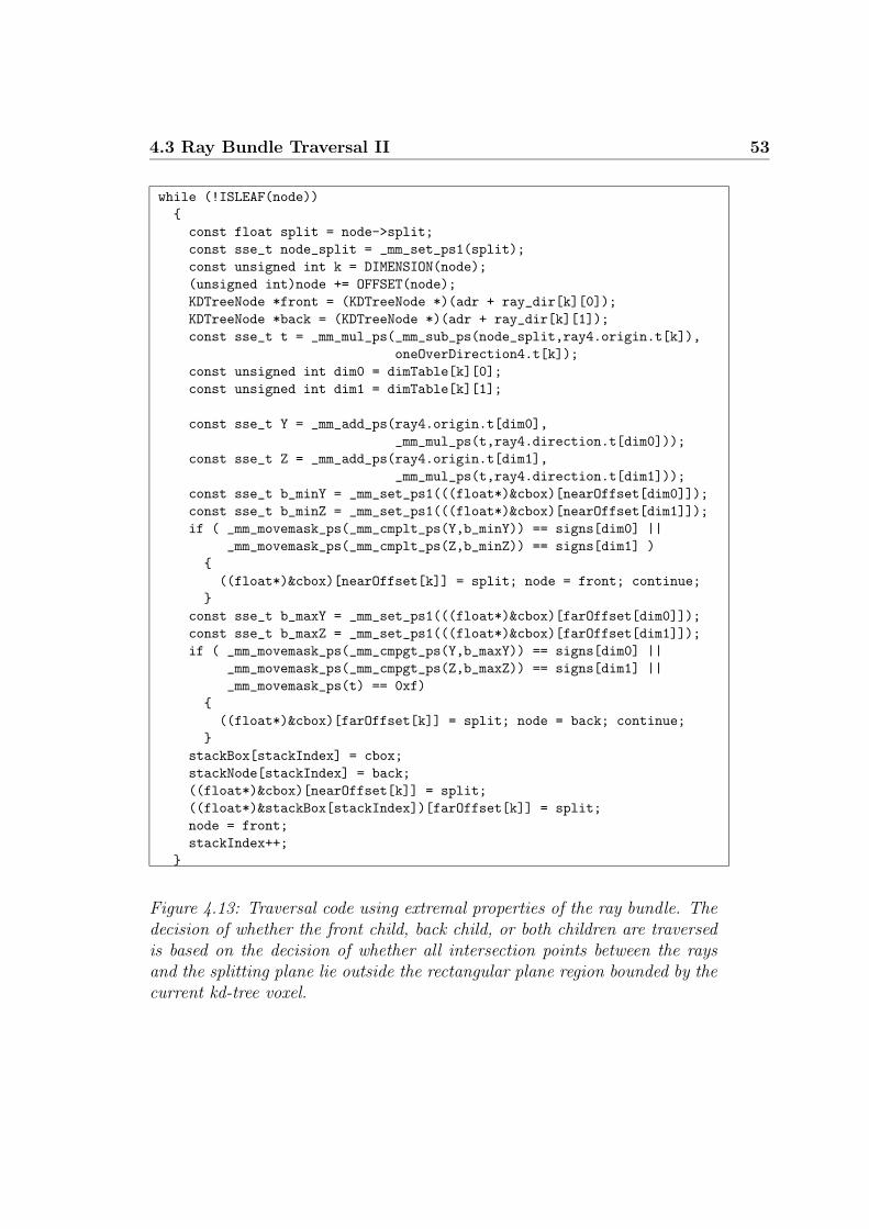
4.3 Ray Bundle Traversal II 53
while (!ISLEAF(node))
{
const float split = node->split;
const sse_t node_split = _mm_set_ps1(split);
const unsigned int k = DIMENSION(node);
(unsigned int)node += OFFSET(node);
KDTreeNode *front = (KDTreeNode *)(adr + ray_dir[k][0]);
KDTreeNode *back = (KDTreeNode *)(adr + ray_dir[k][1]);
const sse_t t = _mm_mul_ps(_mm_sub_ps(node_split,ray4.origin.t[k]),
oneOverDirection4.t[k]);
const unsigned int dim0 = dimTable[k][0];
const unsigned int dim1 = dimTable[k][1];
const sse_t Y = _mm_add_ps(ray4.origin.t[dim0],
_mm_mul_ps(t,ray4.direction.t[dim0]));
const sse_t Z = _mm_add_ps(ray4.origin.t[dim1],
_mm_mul_ps(t,ray4.direction.t[dim1]));
const sse_t b_minY = _mm_set_ps1(((float*)&cbox)[nearOffset[dim0]]);
const sse_t b_minZ = _mm_set_ps1(((float*)&cbox)[nearOffset[dim1]]);
if ( _mm_movemask_ps(_mm_cmplt_ps(Y,b_minY)) == signs[dim0] ||
_mm_movemask_ps(_mm_cmplt_ps(Z,b_minZ)) == signs[dim1] )
{
((float*)&cbox)[nearOffset[k]] = split; node = front; continue;
}
const sse_t b_maxY = _mm_set_ps1(((float*)&cbox)[farOffset[dim0]]);
const sse_t b_maxZ = _mm_set_ps1(((float*)&cbox)[farOffset[dim1]]);
if ( _mm_movemask_ps(_mm_cmpgt_ps(Y,b_maxY)) == signs[dim0] ||
_mm_movemask_ps(_mm_cmpgt_ps(Z,b_maxZ)) == signs[dim1] ||
_mm_movemask_ps(t) == 0xf)
{
((float*)&cbox)[farOffset[k]] = split; node = back; continue;
}
stackBox[stackIndex] = cbox;
stackNode[stackIndex] = back;
((float*)&cbox)[nearOffset[k]] = split;
((float*)&stackBox[stackIndex])[farOffset[k]] = split;
node = front;
stackIndex++;
}
Figure 4.13: Traversal code using extremal properties of the ray bundle. Thedecision of whether the front child, back child, or both children are traversedis based on the decision of whether all intersection points between the raysand the splitting plane lie outside the rectangular plane region bounded by thecurrent kd-tree voxel.
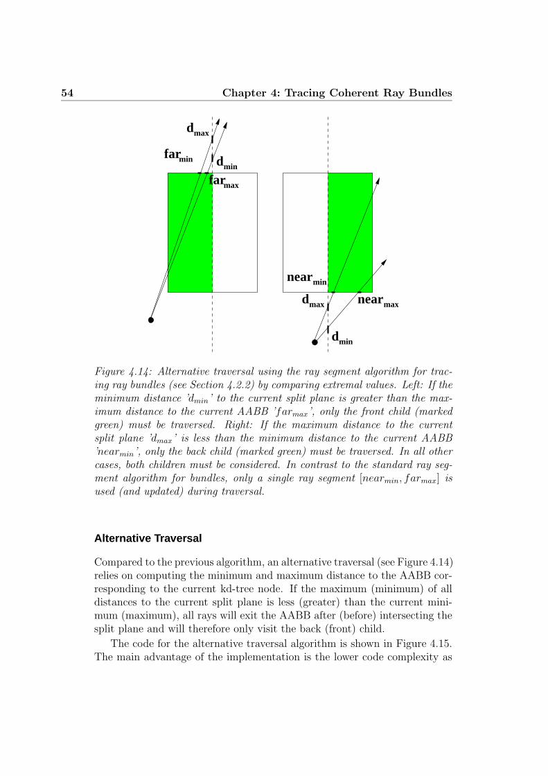
54 Chapter 4: Tracing Coherent Ray Bundles
d
d
min
near
dmax
farmin
farmax
minnear
maxd
min
max
Figure 4.14: Alternative traversal using the ray segment algorithm for trac-ing ray bundles (see Section 4.2.2) by comparing extremal values. Left: If theminimum distance ’dmin’ to the current split plane is greater than the max-imum distance to the current AABB ’farmax’, only the front child (markedgreen) must be traversed. Right: If the maximum distance to the currentsplit plane ’dmax’ is less than the minimum distance to the current AABB’nearmin’, only the back child (marked green) must be traversed. In all othercases, both children must be considered. In contrast to the standard ray seg-ment algorithm for bundles, only a single ray segment [nearmin, farmax] isused (and updated) during traversal.
Alternative Traversal
Compared to the previous algorithm, an alternative traversal (see Figure 4.14)relies on computing the minimum and maximum distance to the AABB cor-responding to the current kd-tree node. If the maximum (minimum) of alldistances to the current split plane is less (greater) than the current mini-mum (maximum), all rays will exit the AABB after (before) intersecting thesplit plane and will therefore only visit the back (front) child.
The code for the alternative traversal algorithm is shown in Figure 4.15.The main advantage of the implementation is the lower code complexity as

4.3 Ray Bundle Traversal II 55
compared to the previous implementations for tracing ray bundles. Sinceonly a single ray segment based on extremal values is used, the algorithmwill introduce unnecessary traversal steps in the case of low ray coherencewithin the bundle.
Note that for further optimization, the horizontal operation within thecode shown in Figure 4.15 can be removed by using a precomputed table ofminimum and maximum values of 1/ray.direction for determining dMin anddMax.
// float near: the current minimum of all distances
// float far: the current maximum of all distances
while (!ISLEAF(node))
{
const float split = node->split;
const sse_t node_split = _mm_set_ps1(split);
const unsigned int k = DIMENSION(node);
adr += OFFSET(node);
KDTreeNode *front = (KDTreeNode *)(adr + ray_dir[k][0]);
KDTreeNode *back = (KDTreeNode *)(adr + ray_dir[k][1]);
const sse_t d = _mm_mul_ps(_mm_sub_ps(node_split,ray4.origin.t[k]),
oneOverDirection4.t[k]);
const float dMin = _mm_cvtss_f32(sseHorizontalMin(d));
const float dMax = _mm_cvtss_f32(sseHorizontalMax(d));
node = back;
if ( dMax < near) { continue; }
node = front;
if ( dMin > far) { continue; }
stack[stackIndex] = back;
stack[stackIndex].near = MAX(dMin,near);
stack[stackIndex].far = far;
stackIndex++;
far = MIN(dMax,far);
}
Figure 4.15: Alternative traversal variant for handling ray bundles by ex-tremal values. The code is based on comparing the extremal distances ’dMin’and ’dMax’ (to a splitting plane) with a single ray segment [near, far].
4.3.3 kd-Tree Entry Point Search
Reshetov et al. [Reshetov05] proposed to use one of the two previous extremaltraversal algorithms to find better entry points within the kd-tree. Havingdeep entry points within the kd-tree allows for minimizing the required num-ber of traversal steps per bundle.

56 Chapter 4: Tracing Coherent Ray Bundles
A
B C
D
F
E
G
inner node
empty leaf
non-empty leaf
Figure 4.16: Simple example of finding a kd-tree entry point for a bundle ofrays using extremal traversal: Starting at the root node ’A’, only the left child’B’ has to be traversed. At ’B’, both children have to be considered. Therefore,’B’ is pushed onto the bifurcation stack, and the traversal continues with thefront child ’D’ of ’B’. At ’D’, only the right child ’G’ has to be traversed. Nodethat ’G’ is a non-empty leaf (marked red), so it becomes the first kd-tree entrypoint candidate and the bifurcation stack is frozen. As the bifurcation stack isnon-empty (it contains ’B’), the entry point algorithm takes a node from thebifurcation stack and continues with its back child (the front child has alreadybeen traversed). The back child ’E’ is an empty leaf (marked green), so thecurrent kd-tree entry point candidate is not updated. As ’E’ is a leaf and thebifurcation stack is empty, the current candidate ’G’ is returned as the kd-treeentry point. In the event that the entry point is already a leaf, which holdstrue for ’G’, only primitive intersection tests need to be performed (skippingray bundle traversal).
The idea behind the kd-tree entry point search is to start with a frustumthat defines the traversal behavior of a bundle of contained rays. For primaryrays generated by a standard perspective camera, the corner rays of a smallN ×N pixel tile will define an appropriate frustum. The ray frustum is tra-versed through the kd-tree until a non-empty leaf is found (see Figure 4.16),or more precisely, until the axis-aligned bounding box of all primitives withinthe non-empty leaf is intersected by the frustum. During traversal, all bifur-cation kd-tree nodes (all nodes where both children have to be considered)

4.3 Ray Bundle Traversal II 57
are pushed onto a stack. This stack (including the first non-empty leaf) con-tains all potential kd-tree entry point candidates. The algorithm continues bytaking a potential candidate from the stack and traversing the correspondingback child (the front child has already been traversed). If for an entry candi-date a non-empty leaf is found, the corresponding bifurcation node becomesthe current entry point candidate. The traversal and candidate updatingcontinues until the stack is empty, all rays within the frustum intersect theprimitives of a non-empty leaf, or a leaf is empty but is marked as insidesome “watertight” object (“empty occluders”) [Reshetov05]. In all cases, thecurrent candidate is returned as an entry point. Since not all rays withinthe frustum have to be defined at the point where the frustum is tested fortermination, the intersection test must rely on the properties of the frustum,i.e. if the frustum misses a primitive, all rays within the frustum will missthe primitive too.
In addition to returning the kd-tree entry point, the algorithm must alsoreturn the corresponding kd-tree cell as an axis-aligned bounding box. Sub-sequent traversal algorithms are initialized by this AABB. An inaccurateAABB, as for example the scene bounding box, will cause unnecessary traver-sal overhead. Note that in the case of ray segment-based traversal, the cor-responding ray clipping step must be performed with the AABB returned bythe kd-tree entry point algorithm.
With respect to a given ray frustum, the kd-tree entry point algorithmreturns either the first bifurcation node, or in the event the bifurcation nodeis empty, the leaf where all rays have ended. The complete sub-tree abovethe entry point can be excluded for the entire set of rays which are boundedby the frustum. The more coherent the rays are, the deeper the entry pointis located within the kd-tree. This allows for efficiently reducing the numberof traversal steps required for the remaining set of rays. In order to achievegood entry points, Reshetov [Reshetov05] suggested to start (for primaryrays) with boundary rays for a fairly large set of rays to continuously createsmaller sets, and to find respective entry points for them. Section 4.4 presentsthe corresponding results when the entry point algorithm is used for primaryrays.
Compared to a standard traversal of ray bundles, the entry point algo-rithm does not perform any intersection test because usually not all rayshave been defined at this point. For the actual implementation, both traver-sal variants shown in Figure 4.13 and Figure 4.15 can be used (with themodification of storing the parent kd-tree node on the stack, instead of thenode referring to the back child). Note that the latter procedure results ina more inaccurate traversal because of using and continuously updating asingle ray segment of extremal values. The inaccurate traversal will typically
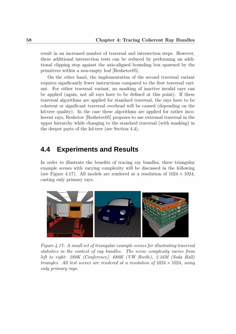
58 Chapter 4: Tracing Coherent Ray Bundles
result in an increased number of traversal and intersection steps. However,these additional intersection tests can be reduced by performing an addi-tional clipping step against the axis-aligned bounding box spawned by theprimitives within a non-empty leaf [Reshetov05].
On the other hand, the implementation of the second traversal variantrequires significantly fewer instructions compared to the first traversal vari-ant. For either traversal variant, no masking of inactive invalid rays canbe applied (again, not all rays have to be defined at this point). If thesetraversal algorithms are applied for standard traversal, the rays have to becoherent or significant traversal overhead will be caused (depending on thekd-tree quality). In the case these algorithms are applied for rather inco-herent rays, Reshetov [Reshetov05] proposes to use extremal traversal in theupper hierarchy while changing to the standard traversal (with masking) inthe deeper parts of the kd-tree (see Section 4.4).
4.4 Experiments and Results
In order to illustrate the benefits of tracing ray bundles, three triangularexample scenes with varying complexity will be discussed in the following(see Figure 4.17). All models are rendered at a resolution of 1024 × 1024,casting only primary rays.
Figure 4.17: A small set of triangular example scenes for illustrating traversalstatistics in the context of ray bundles. The scene complexity varies fromleft to right: 280K (Conference), 680K (VW Beetle), 2.16M (Soda Hall)triangles. All test scenes are rendered at a resolution of 1024 × 1024, usingonly primary rays.

4.4 Experiments and Results 59
4.4.1 Ray Bundle Sizes
Table 4.1 shows traversal and intersection statistics for different ray bundlesizes. These statistics have been generated for the VW Beetle scene usingthe standard ray-segment algorithm shown in Figure 4.9.
Rays/Bundle 1 2 × 2 4 × 4 8 × 8 16 × 16 32 × 32
T Steps/Bundle 29.79 32.25 36.81 56.33 104.32 261.23T Steps/Ray 29.79 8.06 2.3 0.88 0.41 0.26Only Front Side % 36.39 35.80 34.66 31.97 27.34 22.68Only Back Side % 39.08 38.22 36.01 31.65 25.23 19.22Both Sides % 24.53 25.97 29.33 36.39 47.43 58.10I Steps/Bundle 2.73 3.59 5.61 11.68 29.34 88.50
Table 4.1: Traversal and intersection statistics (for primary rays) in relationto different ray bundle sizes. Even though the statistics are generated fromthe VW Beetle model (see Figure 4.17), the two other scenes show a similarbehavior. The average traversal steps per ray (T Steps/Ray) can be signif-icantly reduced by using ray bundles (T Steps/Bundle), while the numberof required intersection steps (I Steps/Bundle) increases for larger bundles.Given the higher intersection than traversal costs, a moderate ray bundle sizeof 4× 4 rays offers the best compromise between traversal step reduction andintersection overhead.
While the total number of traversal steps for a complete frame can beefficiently reduced by using larger ray bundles, the total performance ad-vantage decreases due to the traversal and intersection overhead caused bynon-coherent rays. Because of the overhead, the average number of intersec-tions per bundle (I Steps/Bundle) increases significantly with a larger bundlesize. The impact of traversal overhead for larger bundles can be clearly de-rived from the relative percentage of the three traversal cases (front child,back child, or both children). Using small bundles almost 75% of the casesrequire only the traversal of either the front or the back child. This amountdecreases to 41% for 32 × 32 bundles.
Because of the generally higher costs for intersection than for traversal,a compromise between traversal reduction and intersection overhead has tobe found. The chosen bundle size depends on the cost for a traversal step,the cost for an intersection step, and the quality of the kd-tree itself. For thealgorithms presented here, and the target resolution of 1024×1024, a bundlesize of 4 × 4 rays was found to be most suitable.
If the bounding box of all primitives within a leaf is available, an addi-

60 Chapter 4: Tracing Coherent Ray Bundles
tional clipping step between the bounding box and sub-sets of the ray bundlecan be applied. Assuming for example a bundle size of 8 × 8, additionalclipping tests against the four 4 × 4 bundles could be used to avoid unnec-essary intersection computations. This could further reduce the number ofintersection tests per bundle while introducing additional computations pernon-empty leaf.
4.4.2 Applying kd-Tree Entry Point Search
Finding better kd-tree entry points using the algorithms from Figure 4.13and Figure 4.15, allows for further reducing the number of traversal stepsper bundle. In order to simplify matters, the termination criteria of the kd-tree entry search have been reduced to a simple leaf emptiness test, ignoringadvanced criteria such as “empty occluders”.
For primary rays, the ray frustum is done by splitting the screen into astarting set of 64 × 64 pixel tiles. After looking for a kd-tree entry point byperforming an entry search using the ray frustum of a 64× 64 tile (assuminga standard perspective camera for generating primary rays, these extremalvalues correspond to the corner rays), the tile is split again into a set of 16sub-tiles with a size of 16 × 16 pixels. For each of these 16 × 16 pixel tiles,the entry point search is continued by using the entry point of the preceding64 × 64 tile. At this point, the entry search is finished, and the standardtraversal is invoked. Therefore, each 16 × 16 sub-tile is split once more into16 tiles of 4 × 4 pixel, and a standard traversal algorithm starts with theentry point returned by the entry search of the 16 × 16 tile.
For the three example scenes, the average number of traversal steps per4×4 bundle can be reduced by up to 48% (see Table 4.2). By fine-tuning theheuristics used for the kd-tree construction for individual scenes (e.g. by vary-ing the threshold for cutting off empty space), the reduction can be furtherincreased to over 50% percent. Note that the kd-tree heuristics (e.g. maxi-mum depth criteria or empty space thresholds) for one particular scene arelikely to be sub-optimal for others. This should make it clear that the re-sults achieved by applying kd-tree entry points algorithms depend largelyon the quality of the constructed kd-tree itself. Moreover, the integrationof more sophisticated termination criteria for the kd-tree entry point search,e.g. through inserting empty occluders [Reshetov05] should provide even bet-ter entry points, and therefore a larger reduction of the required traversalsteps.
Note that the 48% of saved traversel steps are only achieved for sceneswith a rather high geometric occlusion, as for example the conference scene.Figure 4.18 visualizes kd-tree entry points for this scene. Almost all primary

4.4 Experiments and Results 61
Figure 4.18: Left Image: Original conference scene with simple shading,Right Image: Visualization of kd-tree entry points. All primary rays cor-responding to the green shaded regions take advantage of kd-tree entry pointswhich are deeper than the root of the tree. The red colored regions refer to en-try points which directly correspond to a single kd-tree leaf. In this case, onlyintersection operations need to be applied and initial operations, e.g. traver-sal initialization or ray clipping can be omitted, saving many unnecessaryoperations.
ray bundles exploit deep kd-tree entry points and even for a fairly largenumber the entry points correspond directly to kd-tree leaf nodes. In thiscase, no traversal but only intersection operations have to be performed.If this case is applied prior to the actual ray bundle traversal, all initialoperations, e.g. ray clipping or traversal initialization can be omitted, thussaving many unnecessary operations. As this optimization technique is ratherspecial, it is not included in any upcoming measurement.
For scenes with high occlusion the effect of using deep kd-tree entry pointscan even save more than half of the traversal steps. Reshetov [Reshetov05]showed that for such scenes, up to 2/3 of all traversal steps can be omitted.On the other hand, complex scenes with less occlusion, such as the VWBeetle scene, are not well-suited for the entry point algorithm. In this case,only a traversal step saving of 20% to 30% is achieved (see Table 4.2).
Table 4.2 also provides statistics for replacing the standard 4 × 4 bundletraversal algorithm (XP) by a version that is similar to the extremal traver-sal algorithms (XP4 ), known from the kd-tree entry search (see Figure 4.13).
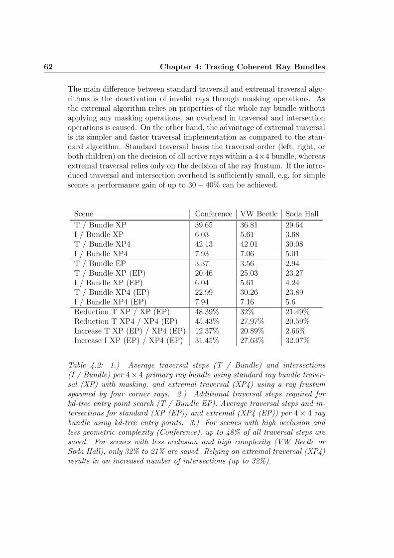
62 Chapter 4: Tracing Coherent Ray Bundles
The main difference between standard traversal and extremal traversal algo-rithms is the deactivation of invalid rays through masking operations. Asthe extremal algorithm relies on properties of the whole ray bundle withoutapplying any masking operations, an overhead in traversal and intersectionoperations is caused. On the other hand, the advantage of extremal traversalis its simpler and faster traversal implementation as compared to the stan-dard algorithm. Standard traversal bases the traversal order (left, right, orboth children) on the decision of all active rays within a 4×4 bundle, whereasextremal traversal relies only on the decision of the ray frustum. If the intro-duced traversal and intersection overhead is sufficiently small, e.g. for simplescenes a performance gain of up to 30 − 40% can be achieved.
Scene Conference VW Beetle Soda Hall
T / Bundle XP 39.65 36.81 29.64I / Bundle XP 6.03 5.61 3.68T / Bundle XP4 42.13 42.01 30.08I / Bundle XP4 7.93 7.06 5.01T / Bundle EP 3.37 3.56 2.94T / Bundle XP (EP) 20.46 25.03 23.27I / Bundle XP (EP) 6.04 5.61 4.24T / Bundle XP4 (EP) 22.99 30.26 23.89I / Bundle XP4 (EP) 7.94 7.16 5.6Reduction T XP / XP (EP) 48.39% 32% 21.49%Reduction T XP4 / XP4 (EP) 45.43% 27.97% 20.59%Increase T XP (EP) / XP4 (EP) 12.37% 20.89% 2.66%Increase I XP (EP) / XP4 (EP) 31.45% 27.63% 32.07%
Table 4.2: 1.) Average traversal steps (T / Bundle) and intersections(I / Bundle) per 4× 4 primary ray bundle using standard ray bundle traver-sal (XP) with masking, and extremal traversal (XP4) using a ray frustumspawned by four corner rays. 2.) Additional traversal steps required forkd-tree entry point search (T / Bundle EP). Average traversal steps and in-tersections for standard (XP (EP)) and extremal (XP4 (EP)) per 4 × 4 raybundle using kd-tree entry points. 3.) For scenes with high occlusion andless geometric complexity (Conference), up to 48% of all traversal steps aresaved. For scenes with less occlusion and high complexity (VW Beetle orSoda Hall), only 32% to 21% are saved. Relying on extremal traversal (XP4)results in an increased number of intersections (up to 32%).
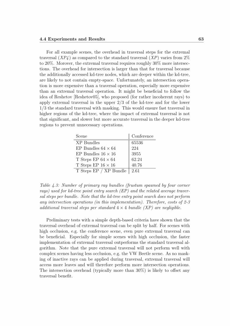
4.4 Experiments and Results 63
For all example scenes, the overhead in traversal steps for the extremaltraversal (XP4 ) as compared to the standard traversal (XP) varies from 2%to 20%. Morover, the extremal traversal requires roughly 30% more intersec-tions. The overhead for intersection is larger than that for traversal becausethe additionally accessed kd-tree nodes, which are deeper within the kd-tree,are likely to not contain empty-space. Unfortunately, an intersection opera-tion is more expensive than a traversal operation, especially more expensivethan an extremal traversal operation. It might be beneficial to follow theidea of Reshetov [Reshetov05], who proposed (for rather incoherent rays) toapply extremal traversal in the upper 2/3 of the kd-tree and for the lower1/3 the standard traversal with masking. This would ensure fast traversal inhigher regions of the kd-tree, where the impact of extremal traversal is notthat significant, and slower but more accurate traversal in the deeper kd-treeregions to prevent unnecessary operations.
Scene Conference
XP Bundles 65536EP Bundles 64 × 64 224EP Bundles 16 × 16 3955T Steps EP 64 × 64 62.24T Steps EP 16 × 16 40.76T Steps EP / XP Bundle 2.61
Table 4.3: Number of primary ray bundles (frustum spawned by four cornerrays) used for kd-tree point entry search (EP) and the related average traver-sal steps per bundle. Note that the kd-tree entry point search does not performany intersection operations (in this implementation). Therefore, costs of 2-3additional traversal steps per standard 4 × 4 bundle (XP) are negligible.
Preliminary tests with a simple depth-based criteria have shown that thetraversal overhead of extremal traversal can be split by half. For scenes withhigh occlusion, e.g. the conference scene, even pure extremal traversal canbe beneficial. Especially for simple scenes with high occlusion, the fasterimplementation of extremal traversal outperforms the standard traversal al-gorithm. Note that the pure extremal traversal will not perform well withcomplex scenes having less occlusion, e.g. the VW Beetle scene. As no mask-ing of inactive rays can be applied during traversal, extremal traversal willaccess more leaves and will therefore perform more intersection operations.The intersection overhead (typically more than 30%) is likely to offset anytraversal benefit.

64 Chapter 4: Tracing Coherent Ray Bundles
The overhead for extremal traversal largely depends on the underlying kd-tree. If the kd-tree is not constructed well, e.g. without applying surface areaheuristics (SAH), the resulting amount of required traversal and intersectionoperations can be tremendous [Havran01, Wald04]. Even in the case of SAH-based kd-tree construction, it is highly beneficial to further optimize thekd-tree for extremal traversal, e.g. by avoiding many extreme small voxels.Reshetov et al. [Reshetov05] proposed several techniques for optimizing SAH-based kd-tree construction, which could additionally lower the traversal andintersection overhead.
In terms of entry search complexity, only 2− 3 additional traversal stepsper 4 × 4 bundle have to be applied (see Table 4.3). Note that the entrypoint search does not perform any intersection operations, so the costs forkd-tree entry search depend exclusively on the traversal costs. The costs forapplying these 2 − 3 additional traversal steps per 4 × 4 bundle are rathernegligible, because these steps are significantly faster than standard traversalsteps.
As the actual ray tracing performance does not only depend on the chosentraversal algorithm but also on the chosen intersection algorithm, all totalperformance statistics for the triangular example scenes are postponed untilChapter 5.
4.4.3 Traversal Costs
Measuring the average cost including memory access for a single traversal stepof a 4 × 4 ray bundle while using the ray-segment code from Section 4.2.3,yields 130 to 220 cycles. The first value was measured on one of the lat-est EM64T architectures with 16 SSE registers, while the second value wasmeasured on a standard 32-bit processor with only 8 SSE registers. This il-lustrates the importance of holding the majority of relevant data within pro-cessor registers as opposed to loading the data from memory. Besides a largernumber of registers, the latest processor generations offer additional featuressuch as improved branch prediction or lower instruction latency which alsohelps.
The observation of improved performance on the latest architectures holdsalso true for the kd-tree entry search algorithm of Section 4.3. Here, thecycle costs vary between 70 and 180 cycles for a single traversal step. Theless complex code results directly in lower cycle costs, and can benefit froma larger number of registers in the same way as the standard 4× 4 traversal.
Amortizing the cycle costs for the standard 4×4 ray bundle traversal overthe number of rays yields 8.13 to 13.75 cycles, which is very low compared tothe traversal costs of 30 cycles for single rays [Wald04]. If a 4×4 ray bundle is

4.4 Experiments and Results 65
traversed using the extremal traversal, the amortized costs are 4.38 to 11.25.All these cycle costs should not be seen as exact calculations but rather as
rough estimates. Given the varying costs of memory access and out-of-orderexecution, an exact timing is very difficult to achieve.
4.4.4 Efficient Mailboxing
Due to the fact that a reference to the same primitive can exist in multiplekd-tree leaves, a ray bundle could perform the primitive intersection testmultiple times. A simple technique to avoid such unnecessary intersectiontests is Mailboxing [Amanatides87, Glassner89, Kirk91].
Mailboxing allows for checking if a given primitive has already been in-tersected by the current ray bundle or not. Therefore, mailboxing requiresthat a unique ID be assigned to each ray bundle. After an intersection test,the primitive is marked as already intersected by assigning the current raybundle ID to the primitive.
Unnecessary tests can now be avoided by performing a simple check beforeevery potential primitive intersection: If the current ray bundle ID matchesthe ID assigned to the primitive candidate, an intersection test between theray bundle and the primitive has already been performed and can thereforebe omitted.
Scene Conference VW Beetle Soda Hall
I Ops/Bundle without MB 6.99 8.17 4.25I Ops/Bundle with MB 5.97 5.45 3.68Reduction 14.59% 33.29% 13.41%
Table 4.4: Average number of intersection tests per 4 × 4 ray bundle withand without standard mailboxing. Applying mailboxing can save 13− 33% ofintersection tests. If the cost for intersection is significantly larger than thecost of traversal, the reduced amount of intersection tests can largely enhanceray tracing performance.
Table 4.4 shows that for the three example scenes, mailboxing allows forreducing the amount of intersection tests per bundle between 13−33%, whichdirectly corresponds to the amount of multiple intersections. The impact ofmailboxing depends largely on the occlusion within the scene and the qualityof the corresponding kd-tree.
As an additional ray bundle ID is required per primitive, the standardmailboxing requires a separate look-up table with a size equal to the number

66 Chapter 4: Tracing Coherent Ray Bundles
unsigned int mbox[NUMBER_OF_PRIMITIVES];
inline void MarkIntersection(const unsigned int triId,
const unsigned int rayId)
{ mbox[triId] = rayId; };
inline bool AlreadyIntersected(const unsigned int triId,
const unsigned int rayId)
{ return mbox[triId] == rayId; };
Figure 4.19: An example implementation for standard mailboxing. The’mbox’ look-up table stores for each primitive the last ray bundle ID (’rayId’)with which an intersection test was performed. Prior to a potential intersec-tion, the primitive ID is taken to determine the entry location and a compar-ison between the current and the stored ray bundle ID is performed. If thesetwo IDs match, an intersection with this primitive has already been performedand can therefore be omitted.
of primitives. Figure 4.19 shows an example implementation for standardmailboxing. Unfortunately, this approach is suboptimal for current CPUarchitectures because the mailbox entries are accessed at almost randomorder, introducing a lot of L2 cache misses. A 1, 000, 000 primitive scenerequires, for example, a mailbox look-up table of 1, 000, 000 ∗ 4 = 3.81 MB,which is larger than any L2 cache. Only a fraction of the complete mailboxcan be held in the L2 cache and the probability that only the cached mailboxentries are accessed is rather low. Besides the actual cache misses, loadingentries out of the mailbox table into the L2 cache overwrites potential kd-treeor any other required data. This can implicitly affect performance of othercomponents of the ray tracing algorithm.
Given the problematic cache behavior a more compact mailbox layout isbeneficial. Fortunately, statistical analyses have shown that a look-up ta-ble with a size equal to the number of primitives is not mandatory becausea ray bundle typically accesses only a subset of all primitives during raytraversal. Therefore, a significantly reduced mailbox look-up table combinedwith a hashing function has proven superior. The mailbox entry is foundby building a hash value with the primitive ID. Each mailbox entry storesthe ray bundle and primitive ID of the last intersection together. Prior to apotential intersection, the ray bundle ID and the primitive ID are tested forequality. Figure 4.20 shows an example implementation for hashed mailbox-ing. Choosing a hash table size of a power of two allows for implementingthe hash function as a simple logical and operation.
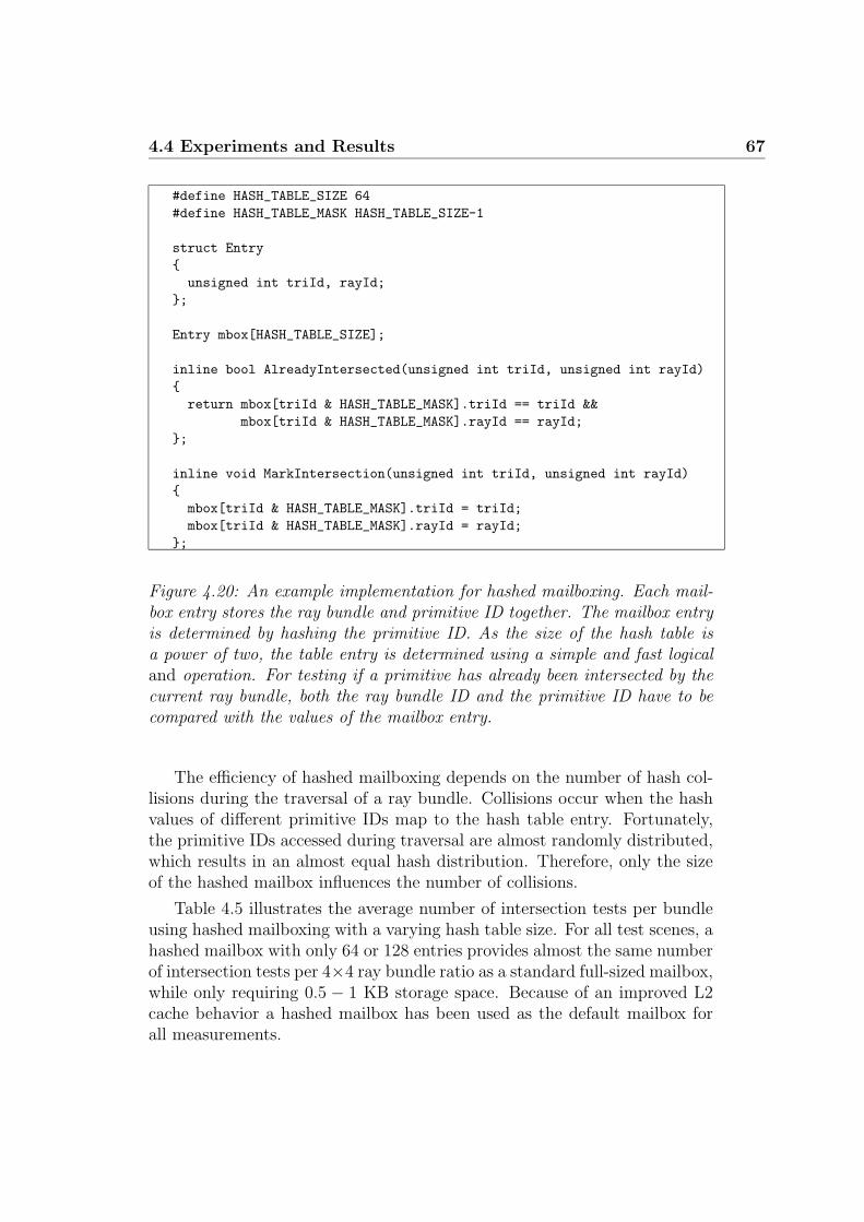
4.4 Experiments and Results 67
#define HASH_TABLE_SIZE 64
#define HASH_TABLE_MASK HASH_TABLE_SIZE-1
struct Entry
{
unsigned int triId, rayId;
};
Entry mbox[HASH_TABLE_SIZE];
inline bool AlreadyIntersected(unsigned int triId, unsigned int rayId)
{
return mbox[triId & HASH_TABLE_MASK].triId == triId &&
mbox[triId & HASH_TABLE_MASK].rayId == rayId;
};
inline void MarkIntersection(unsigned int triId, unsigned int rayId)
{
mbox[triId & HASH_TABLE_MASK].triId = triId;
mbox[triId & HASH_TABLE_MASK].rayId = rayId;
};
Figure 4.20: An example implementation for hashed mailboxing. Each mail-box entry stores the ray bundle and primitive ID together. The mailbox entryis determined by hashing the primitive ID. As the size of the hash table isa power of two, the table entry is determined using a simple and fast logicaland operation. For testing if a primitive has already been intersected by thecurrent ray bundle, both the ray bundle ID and the primitive ID have to becompared with the values of the mailbox entry.
The efficiency of hashed mailboxing depends on the number of hash col-lisions during the traversal of a ray bundle. Collisions occur when the hashvalues of different primitive IDs map to the hash table entry. Fortunately,the primitive IDs accessed during traversal are almost randomly distributed,which results in an almost equal hash distribution. Therefore, only the sizeof the hashed mailbox influences the number of collisions.
Table 4.5 illustrates the average number of intersection tests per bundleusing hashed mailboxing with a varying hash table size. For all test scenes, ahashed mailbox with only 64 or 128 entries provides almost the same numberof intersection tests per 4×4 ray bundle ratio as a standard full-sized mailbox,while only requiring 0.5 − 1 KB storage space. Because of an improved L2cache behavior a hashed mailbox has been used as the default mailbox forall measurements.

68 Chapter 4: Tracing Coherent Ray Bundles
Scene Conference VW Beetle Soda Hall
Standard Mailbox 5.97 5.45 3.68Hashed Mailbox 16 Entries 6.14 (2.8%) 6.02 (10.4%) 3.79 (2.9%)Hashed Mailbox 32 Entries 6.06 (1.5%) 5.77 (5.8%) 3.76 (2.1%)Hashed Mailbox 64 Entries 6.03 (1.0%) 5.61 (2.9%) 3.73 (1.3%)Hashed Mailbox 128 Entries 6.00 (0.5%) 5.52 (1.2%) 3.72 (1.0%)
Table 4.5: Average number of intersection tests per 4 × 4 ray bundle usinghashed mailboxing with a varying hash table size. A hashed mailbox withonly 64 or 128 entries ensure almost the same ratio (difference of less than3%) as that of a standard full-sized mailbox. As a hashed mailbox with 128entries requires only 1 KB storage space, the probability of a cache misswhen accessing a mailbox entry is significantly lower than that of a standardmailbox.
4.4.5 Shading Coherent Rays
Supporting the efficient bundling of coherent rays in a standard recursiveray tracer can be very difficult. Tracing bundles is not problematic for pri-mary rays because those are usually generated in a coherent manner. Also,the coherence of shadow rays traced from the first hit point to a point lightis usually very high. The problem appears when handling secondary rays,especially recursive reflected or refracted rays. For these kinds of rays, co-herence between rays may be lost. Obviously, one could trace a bundle ofincoherent rays. The problem is that with incoherent bundles only a fewrays will be active during traversal, which is likely to offset the performancebenefit of tracing bundles. Therefore, some kind of efficient regrouping willbe necessary.
In standard ray tracing systems the recursive evaluation of secondary rayswithin a freely programmable surface shader is very common. A regroupingoperation for secondary rays is difficult to realize efficiently in software, be-cause a recursive shader evaluation must be temporarily stopped in order toinsert a ray into the appropriate ray bundle, and it must be restarted oncethe bundle has been traced.
One possible solution to this problem is to split the shading model into aprogrammable and a fix function part. The programmable part defines a rayquery and transfers the query to fix part. The queries for a complete bundleare gathered and the fix function part of the shaders traces them together asa bundle. This approach only works for secondary rays which are spawnedby the same surface shader [Benthin03].

4.5 Conclusions and Future Work 69
Woop et al. [Woop05] proposed to handle different shaders for a given setof intersections in a multi-pass way on a ray tracing hardware architecture.For each shader type, an individual pass is performed, excluding intersec-tions of different shaders by masking. This approach does not include anexplicit regrouping of rays because it only groups and traces rays from thesame shader in a bundle (even if the rays are incoherent). The pure hardwareapproach makes it even possible to stop and restart recursive shader evalua-tion without any performance losses. Even though the same approach couldalso be realized in terms of software, it is unclear how effective a softwareimplementation would be.
Even though several approaches for shading coherent rays exist, for apure software system, an efficient algorithm for the regrouping of coherentrays and the design of an efficient shading model for ray bundles remains anopen question to this day.
4.5 Conclusions and Future Work
In summary, current CPU architectures allow for efficient kd-tree traversalif the corresponding implementation has been carefully adapted to the un-derlying hardware. However, traversal implementation will be even faster iffuture CPU architectures offer a higher number of registers, less deep exe-cution pipelines to lower the impact of branch mis-predictions, as well as animproved instruction set.
For the future, it will be very interesting to minimize the traversal and in-tersection overhead for extremal traversal. If the overhead can be minimizedto a similar level as for standard traversal, extremal traversal will be themethod of choice in terms of performance. Besides faster implementation,the costs for extremal traversal are constant because they are independentof the number of rays within the bundle. This will be beneficial in the caselarge bundles of coherent rays need to be traced, e.g. for anti-aliasing bysuper-sampling.

70 Chapter 4: Tracing Coherent Ray Bundles

Chapter 5
Coherent Ray Tracing forTriangular Surfaces
Triangles are essentially the standard geometric representation for renderingin computer graphics. As triangles are the standard primitive for today’sgraphics hardware, scene complexity is predominantly measured in triangles.Typical scene complexity for models used in the context of virtual prototyp-ing, ranges from several hundred thousands to millions of triangles.
As shown in Chapter 4, tracing coherent ray bundles instead of single raysis the key factor for increasing traversal performance. SSE instructions, whichallow for efficient traversal implementation in the context of ray bundles, canalso be applied to speed up triangle intersection.
In order to illustrate ray-triangle intersection algorithms in the context ofcoherent ray bundles, a small collection of triangular scenes have been used(see Chapter 4).
Researchers proposed many algorithms for computing the intersectionbetween a single ray and a triangle [Glassner89, Badouel92, Erickson97,Moller97, Shoemake98, Wald04]. Some of these algorithms require only thevertices of the triangle as input data, others rely on extra precomputed datato ensure maximum performance. In the following sections, the implementa-tions of two of these algorithms are presented in detail in the context of raybundles.
This chapter starts with a presentation of the algorithm proposed by Waldet al. [Wald04] in Section 5.1. In Section 5.2, a variation of the Plueckertest is proposed which has been adapted in order to handle ray bundlesefficiently. Finally, Section 5.3 illustrates the effective combination of fastkd-tree traversal and intersection for ray tracing triangular scenes.

72 Chapter 5: Coherent Ray Tracing for Triangular Surfaces
struct TriAccel
{
// plane:
float n_u; // normal.u / normal.k
float n_v; // normal.v / normal.k
float n_d; // constant of plane equation
int k; // projection dimension
// line equation for line ac
float b_nu;
float b_nv;
float b_d;
int pad0; // pad to 48 bytes for cache alignment purposes
// line equation for line ab
float c_nu;
float c_nv;
float c_d;
int pad1; // pad to 48 bytes for cache alignment purposes
};
Figure 5.1: Structure for storing the preprocessed triangle data. It containstriangle data that is projected onto one of the three axis-aligned planes (thecorresponding dimension is indicated by parameter ’k’). The data block re-lated to normal data is used for computing the intersection distance whilethe two other blocks are used for computing the barycentric coordinates. Thepadding to a 48-byte size allows for a better cache access pattern.
5.1 Triangle Intersection I
A fast ray-triangle intersection test which can be efficiently implementedusing SSE instructions was proposed by Wald et al. [Wald04]. The basic ideabehind this test is to project the triangle into one of the three axis-alignedplanes and to perform the computation of the barycentric coordinates in 2Dinstead of 3D. This allows for reducing the number of operations required.In order to ensure maximum performance, the algorithm relies on a smallamount of precomputed data (see Figure 5.1) for every triangle. Relyingon this precomputed data basically avoids additional instructions for datarearrangement, which can be costly using SSE.
The size of the precomputed data per triangle corresponds to 48 bytes,resulting in a tolerable amount of 45.78 MB of additional preprocessed datafor a typical one-million-triangle scene. Additionally, the size of 48 bytes

5.1 Triangle Intersection I 73
corresponds to 1.5 cache-lines for a 32-byte cache-line size, or to 0.75 cache-lines for a 64-byte cache-line.
5.1.1 Implementation
Adapting the original algorithm [Wald04] for supporting four rays in parallelusing SSE instructions is straightforward. Figure 5.2 shows an example im-plementation for four rays. An implementation for 4 × 4 rays can be simplyachieved by sequentially performing the intersection code four times.
A closer look at the code shows that extra shuffle operations are requiredto copy a single float value (from the corresponding preprocessed TriAccelstructure) to all SSE register elements at the beginning. Replicating theTriAccel elements four times would allow for a more suitable access butwould also result in a four times larger structure size. Additionally, thiswould significantly increase the required memory bandwidth and lower theeffect of caches, which is is not beneficial.
The first sequence of instructions computes the distances f between theray origins and the triangle plane using the precomputed normal data in theTriAccel structure. As the distance computation involves a costly divisionand the subsequent instructions depend on the result, the implementationuses a Newton-Raphson iteration for computing the inverse. This allowsfor reducing latency and for better interleaving of surrounding instructions(increased instruction level parallelism). The slightly less accurate resultcompared to a real division is negligible.
Comparing the four distances f with the previous intersection distancesforms the first potential exit point. Note that the exit is only taken if thecomparison holds true for all four rays. This is an example for decisioncoherence. The higher the coherence of the rays, the higher the probabilitythat all rays leave the code sequence at a given exit point.
The subsequent instructions basically compute the barycentric coordi-nates and compare the results to the valid bounds for a triangle. The secondand third exit points require the results of the barycentric coordinate compu-tation and are therefore located in the middle and at the end of the algorithm.After the fourth, and final exit point the data for the four intersections isupdated according to the accumulated final mask.
A size of 48 bytes and a data alignment that is a multiple of the cache-line size ensures that for accessing all required data only one cache-line oronly a maximum of two cache-lines (per triangle) must be loaded. A detaileddiscussion about the algorithmic details and the required preprocessing forthe intersection algorithm is given in [Wald04].
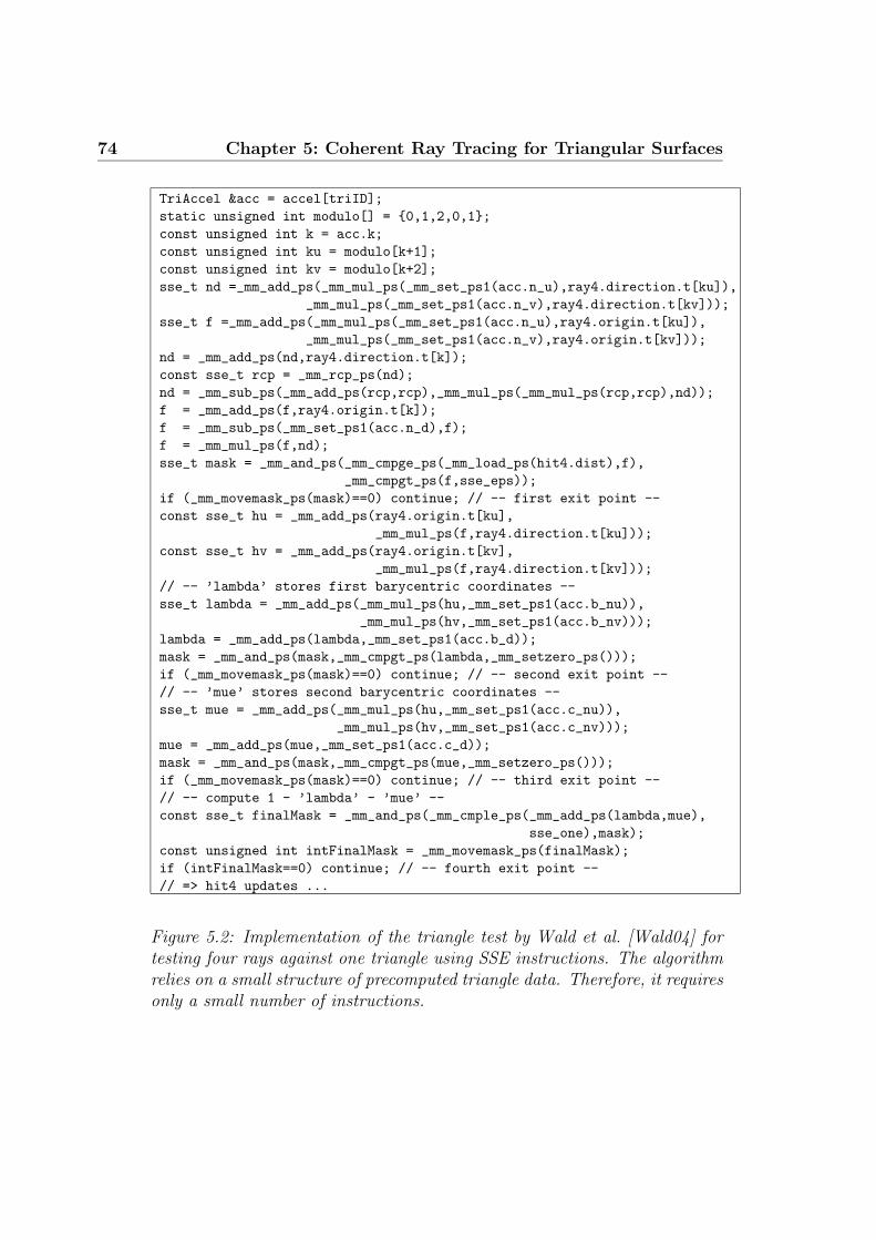
74 Chapter 5: Coherent Ray Tracing for Triangular Surfaces
TriAccel &acc = accel[triID];
static unsigned int modulo[] = {0,1,2,0,1};
const unsigned int k = acc.k;
const unsigned int ku = modulo[k+1];
const unsigned int kv = modulo[k+2];
sse_t nd =_mm_add_ps(_mm_mul_ps(_mm_set_ps1(acc.n_u),ray4.direction.t[ku]),
_mm_mul_ps(_mm_set_ps1(acc.n_v),ray4.direction.t[kv]));
sse_t f =_mm_add_ps(_mm_mul_ps(_mm_set_ps1(acc.n_u),ray4.origin.t[ku]),
_mm_mul_ps(_mm_set_ps1(acc.n_v),ray4.origin.t[kv]));
nd = _mm_add_ps(nd,ray4.direction.t[k]);
const sse_t rcp = _mm_rcp_ps(nd);
nd = _mm_sub_ps(_mm_add_ps(rcp,rcp),_mm_mul_ps(_mm_mul_ps(rcp,rcp),nd));
f = _mm_add_ps(f,ray4.origin.t[k]);
f = _mm_sub_ps(_mm_set_ps1(acc.n_d),f);
f = _mm_mul_ps(f,nd);
sse_t mask = _mm_and_ps(_mm_cmpge_ps(_mm_load_ps(hit4.dist),f),
_mm_cmpgt_ps(f,sse_eps));
if (_mm_movemask_ps(mask)==0) continue; // -- first exit point --
const sse_t hu = _mm_add_ps(ray4.origin.t[ku],
_mm_mul_ps(f,ray4.direction.t[ku]));
const sse_t hv = _mm_add_ps(ray4.origin.t[kv],
_mm_mul_ps(f,ray4.direction.t[kv]));
// -- ’lambda’ stores first barycentric coordinates --
sse_t lambda = _mm_add_ps(_mm_mul_ps(hu,_mm_set_ps1(acc.b_nu)),
_mm_mul_ps(hv,_mm_set_ps1(acc.b_nv)));
lambda = _mm_add_ps(lambda,_mm_set_ps1(acc.b_d));
mask = _mm_and_ps(mask,_mm_cmpgt_ps(lambda,_mm_setzero_ps()));
if (_mm_movemask_ps(mask)==0) continue; // -- second exit point --
// -- ’mue’ stores second barycentric coordinates --
sse_t mue = _mm_add_ps(_mm_mul_ps(hu,_mm_set_ps1(acc.c_nu)),
_mm_mul_ps(hv,_mm_set_ps1(acc.c_nv)));
mue = _mm_add_ps(mue,_mm_set_ps1(acc.c_d));
mask = _mm_and_ps(mask,_mm_cmpgt_ps(mue,_mm_setzero_ps()));
if (_mm_movemask_ps(mask)==0) continue; // -- third exit point --
// -- compute 1 - ’lambda’ - ’mue’ --
const sse_t finalMask = _mm_and_ps(_mm_cmple_ps(_mm_add_ps(lambda,mue),
sse_one),mask);
const unsigned int intFinalMask = _mm_movemask_ps(finalMask);
if (intFinalMask==0) continue; // -- fourth exit point --
// => hit4 updates ...
Figure 5.2: Implementation of the triangle test by Wald et al. [Wald04] fortesting four rays against one triangle using SSE instructions. The algorithmrelies on a small structure of precomputed triangle data. Therefore, it requiresonly a small number of instructions.

5.1 Triangle Intersection I 75
5.1.2 Discussion
If one has a closer look at the algorithm from Figure 5.2, it becomes evidentthat the intersection algorithm discards a triangle on the basis of two tests:
Distance Test: The test checks if the potential intersection distance is ina valid range. If for all rays, the intersection distance to the triangleplane is greater than the last valid intersection distance, the trianglecan be excluded from further processing.
Inside Test: The test checks if the rays within a bundle pierce the triangleat all. For the algorithm shown in Figure 5.2, this is done by computingthe barycentric coordinates and testing them to determine whetherthey are in a valid range. If the barycentric coordinates for all raysare outside the valid range, the triangle can be excluded from furtherprocessing.
The inside test takes place very late in the algorithm (essentially at thelast exit point), compared to the distance test. Table 5.1 shows the averageprobabilities for the distance and inside test, together with the probabilitiesfor a full test execution. All test scenes are rendered at a resolution of1024×1024 and with a bundle size of 4×4 rays. A given ray bundle is dividedinto four-ray bundles, each four-ray bundle being processed individually.
Only 20 % to 28 % of all ray bundle tests require a full execution ofthe test. Moreover, 52 % to 68 % of all tests leave execution at the exitpoints related to the inside test, while only roughly 18 % (or less) exit at thedistance test.
Scene Conference VW Beetle Soda Hall
Distance Test Exit % 17.99 13.05 19.30Inside Test Exit % 61.98 68.90 52.32Full Test % 20.03 18.05 28.38
Table 5.1: Average probability for exiting at the distance and inside test aswell as for performing the full test execution. The three example scenes arerendered at a resolution of 1024× 1024 with 16 rays per bundle, casting onlyprimary rays. Approximately 20 % to 28 % of all four-ray bundle intersectiontests require a full test execution. Between 52 % and 68 % of all tests exit atthe inside test and therefore miss the triangle completely.
Moreover, a certain amount of the early exits performed by the distancetest can be handled by the inside test, as shown in Table 5.2. Therefore, the
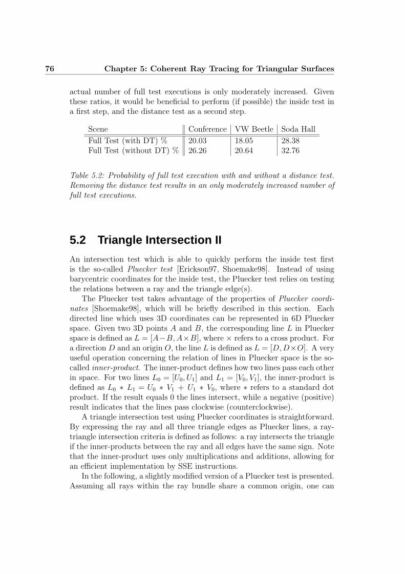
76 Chapter 5: Coherent Ray Tracing for Triangular Surfaces
actual number of full test executions is only moderately increased. Giventhese ratios, it would be beneficial to perform (if possible) the inside test ina first step, and the distance test as a second step.
Scene Conference VW Beetle Soda Hall
Full Test (with DT) % 20.03 18.05 28.38Full Test (without DT) % 26.26 20.64 32.76
Table 5.2: Probability of full test execution with and without a distance test.Removing the distance test results in an only moderately increased number offull test executions.
5.2 Triangle Intersection II
An intersection test which is able to quickly perform the inside test firstis the so-called Pluecker test [Erickson97, Shoemake98]. Instead of usingbarycentric coordinates for the inside test, the Pluecker test relies on testingthe relations between a ray and the triangle edge(s).
The Pluecker test takes advantage of the properties of Pluecker coordi-nates [Shoemake98], which will be briefly described in this section. Eachdirected line which uses 3D coordinates can be represented in 6D Plueckerspace. Given two 3D points A and B, the corresponding line L in Plueckerspace is defined as L = [A−B,A×B], where × refers to a cross product. Fora direction D and an origin O, the line L is defined as L = [D,D×O]. A veryuseful operation concerning the relation of lines in Pluecker space is the so-called inner-product. The inner-product defines how two lines pass each otherin space. For two lines L0 = [U0, U1] and L1 = [V0, V1], the inner-product isdefined as L0 ∗ L1 = U0 ∗ V1 + U1 ∗ V0, where ∗ refers to a standard dotproduct. If the result equals 0 the lines intersect, while a negative (positive)result indicates that the lines pass clockwise (counterclockwise).
A triangle intersection test using Pluecker coordinates is straightforward.By expressing the ray and all three triangle edges as Pluecker lines, a ray-triangle intersection criteria is defined as follows: a ray intersects the triangleif the inner-products between the ray and all edges have the same sign. Notethat the inner-product uses only multiplications and additions, allowing foran efficient implementation by SSE instructions.
In the following, a slightly modified version of a Pluecker test is presented.Assuming all rays within the ray bundle share a common origin, one can
5.2 Triangle Intersection II 77
further optimize the original algorithm [Shoemake98]. Through transferringthe ray origin to the origin of the coordinate system (by subtracting theorigin O from the triangle vertices A and B), the inner-product between theray R = [D,D × O] and the triangle edge E = [A − B,A × B] is simplifiedto
R ∗ E = D ∗ ((A − O) × (B − 0)) + D × (O − O) ∗ ((A − O) − (B − O))
= D ∗ ((A − O) × (B − 0)) + 0 ∗ (A − B)
= D ∗ ((A − O) × (B − 0))
Having a common origin per ray bundle, e.g. for primary rays or forshadow rays to a point light, allows for efficiently amortizing the computationcosts for (A−O)× (B−0) (and the required computations for the remainingtwo edges) over all rays within the bundle. The actual inside test for a four-ray bundle can be performed simply by evaluating three dot products usingSSE instructions.
In order to obtain the intersection distances t, the following equation hasto be evaluated after the edge tests:
t =N ∗ (A − O)
D ∗ N
where N is the triangle normal. As N ∗ (A−O) is fixed for the whole bundleit can also be precomputed. Note that the normal N of each triangle can beprecomputed and stored as preprocessed data during scene definition. Onthe other hand, one can omit the preprocessing and compute all necessarydata on the fly. In terms of changing vertices, e.g. for dynamic animation,this approach can be more efficient than carrying out an extra preprocessingstep.
5.2.1 Implementation
A simplified implementation of the intersection algorithm is shown in Fig-ure 5.3. The Init function is used for precomputing all edge and normal datafor the whole bundle. The actual intersection code starts with the compu-tation of three dot products. The corresponding signs for all three edgesare compared for equality. If no ray indicates a valid intersection, no bit isset in the mask value, and the next ray bundle is processed. If at least oneray has a valid intersection, the execution continues with the computationof intersection distances. The look-up into the sseMaskTable table loads a

78 Chapter 5: Coherent Ray Tracing for Triangular Surfaces
// -- precomputed per bundle --
SSEVec4 v0_cross, v1_cross, v2_cross, normal;
sse_t nominator, triNum;
inline void Init(const R3 &a,const R3 &b,const R3 &c,
const R3 &origin,int id)
{
v1_cross = (b-origin)^(a-origin);
v2_cross = (a-origin)^(c-origin);
v0_cross = (c-origin)^(b-origin);
const R3 n = (c-a)^(b-a); normal = n; // convert R3 -> SSEVec4
nominator = _mm_set_ps1(n * (a-origin));
triNum = _mm_set_ps1(*(float *)&id);
}
inline void Intersect(const SSERay4 *ray4,SSEIntersection4 *hit4)
{
for (unsigned int i=0;i<BUNDLES;i++) {
const sse_t v0d = Dot(v0_cross,ray4[i].direction);
const unsigned int v0s = _mm_movemask_ps(v0d);
const sse_t v1d = Dot(v1_cross,ray4[i].direction);
const unsigned int v1s = _mm_movemask_ps(v1d);
const sse_t v2d = Dot(v2_cross,ray4[i].direction);
const unsigned int v2s = _mm_movemask_ps(v2d);
const unsigned int mask = (v0s & v1s & v2s) |
((v0s^0xf) & (v1s^0xf) & (v2s^0xf));
if ( mask > 0 ) {
const sse_t dist = _mm_mul_ps(nominator,
Inverse(Dot(ray4[i].direction,normal)));
sse_t finalMask = *(sse_t*)&sseMaskTable[mask][0];
const sse_t vol = Inverse(_mm_add_ps(_mm_add_ps(v0d,v1d),v2d));
finalMask = _mm_and_ps(_mm_cmple_ps(dist,*(sse_t*)hit4[i].dist),
finalMask);
finalMask = _mm_and_ps(_mm_cmpge_ps(dist,EPSILON),finalMask);
const sse_t lambda = _mm_mul_ps(v0d,vol);
const sse_t mue = _mm_mul_ps(v2d,vol);
// => update intersection structure: hit4[i]
}
}
}
Figure 5.3: A reliable triangle intersection test based on Pluecker coordinatesadapted for ray bundles with a common origin. A triangle can be pruned earlyby performing only three dot products (one for each edge) using precomputeddata. The cost for preprocessing Pluecker coordinates for all three triangleedges is amortized over the ray bundle.

5.3 Results 79
binary SSE mask. Each of the four lowest bits is replicated 32 times in thecorresponding register element: If, for example, the lowest bit of four bits isset, the lowest element of the SSE register will be set to 0xffffffff , andto 0x00000000 otherwise.
The results of the inner-products can also be used to obtain the barycen-tric coordinates. The three results correspond to the homogeneous barycen-tric coordinates. In order to determine the final coordinates, a division bythe sum of all three coordinate values has to be performed. Note that thedivision does not need to be performed every time, but only once at the endof ray traversal. Note also that this requires all three coordinate values tobe temporarily stored and updated.
The actual computation of intersection distances could also be done with-out an inverse operation. The three barycentric coordinates u, v, w and thetriangle vertices V ertexA, V ertexB, and V ertexC allow for easily determin-ing the intersection point P (u, v, w):
P (u, v, w) = V ertexA ∗ u + V ertexB ∗ v + V ertexC ∗ w
The intersection distance is the projection along the direction of the ray:
distance = ray.direction ∗ (P (u, v, w) − ray.origin)
Unfortunately, the approach of computing the distance by projectionalong the direction is a few percent slower than computing the distance bydivision because of the increased number of instructions required. The ma-jor advantage of the division-free approach is that it exclusively relies onmultiply-add sequences which might be beneficial for future architectures.
5.3 Results
Accurately determining run-time costs in CPU cycles for the different trian-gle intersection algorithms is difficult because of the varying early exit pointprobabilities. For the example scenes shown in Figure 4.17, three cost cat-egories have been defined. The first one measures the cycles until an earlyexit with respect to a triangle test occurs, the second one corresponds to afull test execution, while the third one represents the average cost based onthe probability distribution of the exit points for the particular view.
Table 5.3 presents the cost for all three categories with respect to a bundleof 4 × 4 rays. The numbers in parentheses correspond to the amortized

80 Chapter 5: Coherent Ray Tracing for Triangular Surfaces
Intersection Test Miss Triangle Full Execution Average
Projection (cycles) 420 (26.25) 620 (38.75) 480 (30)Pluecker (cycles) 310 (19.38) 590 (36.88) 385 (24.06)
Table 5.3: Triangle intersection cost in CPU cycles for different executionscenarios. All costs are measured for a bundle of 16 ray, the numbers inbrackets correspond to the amortized costs per ray. The first number givesthe cost if all rays miss the triangle, the second if all rays hit the triangle.The third takes the probability distribution of exit points into account.
cost per ray. Note that for the Pluecker test, the cycle cost includes thepreprocessing step.
If the probability that rays miss the current triangle is high, the Plueckertest is able to play off its strength. Depending on the view and scene, anaverage speedup of up to 25% (for the triangle test) can be achieved comparedto the test by Wald et al. (see Section 5.1). Note that the total speedup ofthe core ray tracing performance lies typically between 2 − 10%, becauseintersection computations take only a certain part of the time (see below).However, for most scenes, the Pluecker intersection test is the fastest forcoherent bundles and is therefore used as the default test for ray tracingtriangular scenes.
One could further optimize the Pluecker test by not executing the testper triangle but by executing it first for all edges and later reusing the resultsfor the triangles. If the ratio of shared triangle edges is high, a significantamount of operations can be saved.
Applying an edge-based intersection has the additional advantage of be-ing reliable in the intersection decision. Due to numerical instabilities anintersection test which relies on the comparison of barycentric coordinatescan produce wrong results at edges of adjacent triangles. In this case, thetest returns a wrong miss which can result in visible artifacts. An edge-basedtest that uses a fixed order of edge vertices is non-ambiguous and thereforereliable.
Combining the techniques for traversal of coherent ray bundles fromChapter 4 with the fast triangle intersection tests for ray bundles allows foreasily achieving interactive ray tracing performance even on a single desktopPC. Table 5.4 illustrates performance statistics using a commodity 2.2 GHzIntel Pentium-IV PC.
Tracing ray bundles allows for achieving interactive performance even ona single CPU system. Applying performance analysis with VTune to the

5.3 Results 81
core ray tracing algorithm shows that roughly 60% of the time is spent ontraversal, while 40% is spent on intersection tests. Good kd-tree entry pointsreduces the required traversal steps per bundle by up to 50%. Reducing thenumber of required traversal steps per bundle shifts the traversal/intersectionratio to 40% for traversal and 60% for intersection. This illustrates that theintersection test is now becoming the limiting factor. Further speed opti-mization should therefore concentrate on speeding up triangle intersection.
Scene (1024 × 1024) Conference VW Beetle Soda Hall
Without Entry Point Search (fps) 3.100 3.150 3.432With Entry Point Search (fps) 4.052 3.556 3.854Speedup 30.71% 12.8% 12.29%
Table 5.4: Performance statistics for triangular scenes rendered at a reso-lution of 1024 × 1024 with a ray bundle size of 4 × 4. All tests were runon a commodity 2.2 GHz Intel Pentium-IV PC, casting only primary rays.The first row illustrates performance statistics without applying kd-tree en-try point search, while the second row takes advantage of entry point search.Even though the entry point search efficiently reduces the required number oftraversal steps per 4 × 4 bundle by up to 50%, the total performance gainis rather small (between 12-30%). The reason for this is that the triangleintersection is more and more becoming the bottleneck: For a typical scene,60% of the ray tracing time is taken up by traversal while 40% is taken upby intersection.
Due to the fact that a resolution of 1024×1024 yields 65536 ray bundles ofthe size 4×4 and each bundle requires an average of 39.49 (conference scene)traversal steps without applying entry point search, the required memorybandwidth for kd-tree nodes is 65536 ∗ 39.49 ∗ 8 = 19.745 MB/frame. Ap-plying the kd-tree entry point algorithm cuts down the number of traversalsteps to 50%, reducing the bandwidth accordingly.
For the intersection tests, the 65536 ray bundles require an average band-width of 6.06 times the size of the triangle intersection data. Applying thetest proposed by Wald et al. [Wald04], requires 48 bytes of precomputed dataper triangle. This results in a total bandwidth of 65536 ∗ 6.06 ∗ 48 = 18.18MB/frame. Therefore, the total required bandwidth of external data sumsup to 37.925 MB/frame. Most of these bandwidths (> 90% percent) can becompensated for due to the multi-level cache hierarchies of current CPUs,which yields an external memory bandwidth of less than 4 MB/frame.

82 Chapter 5: Coherent Ray Tracing for Triangular Surfaces
5.4 Conclusions and Future Work
Section 5.3 showed that the combination of efficient traversal, kd-tree entrypoint search, and triangle intersection for ray bundles allows for achievinginteractive ray tracing even on a single CPU. All tests were run on a 2.2 GHzIntel Pentium-IV processor, more recent CPU versions will therefore achieveeven better results.
As fast ray bundle traversal increases the impact of triangle intersec-tion on the core ray tracing performance, a triangle intersection test for raybundles has been proposed that efficiently prunes non-intersecting triangles.For future implementations, it might be necessary to further speed up theintersection test for coherent ray bundles.
A promising approach to this problem could be to store the triangle ge-ometry as small index face sets instead of individual triangles. In the casea ray bundle enters a leaf, a fast side test, e.g. a Pluecker test, would firstbe performed for all edges. In a second step, the results of the edge testswould be passed to the actual triangle test. Given the high probability ofshared edges within a kd-tree leaf, the total amount of operations per leafcould be reduced. Moreover, the side test would ensure high instruction levelparallelism, because no dependencies exist between the computation of dif-ferent edges. In terms of implementation, a kd-tree leaf would not only storereferences to triangles but additionally references to triangle edges.

Chapter 6
Coherent Ray Tracing forFreeform Surfaces
Almost all CAD systems and design tools rely on freeform surfaces such as B-Splines, NURBS, or subdivision surfaces for representing 3D surfaces. How-ever, almost all commercial ray tracing systems tessellate freeform surfacesinto simpler geometric primitives, e.g. triangles. The tessellation process isusually applied before the actual rendering process starts. Tessellation it-self, and therefore the increased amount of scene data, is often consideredacceptable because ray tracing is known for its logarithmic behavior in scenecomplexity.
In Chapter 5, it has been shown that interactive ray tracing on commodityhardware is possible even when dealing with millions of triangles. It is thuslegitimate to ask why freeform surfaces should be ray traced directly. Theanswer to this question is simple: Tessellating freeform surfaces into triangleshas serious drawbacks:
Scene and Storage Complexity: The amount of required storage spacefor tessellated triangles is orders of magnitudes higher than for theoriginal freeform data.
Accuracy: Tessellation can be seen as producing a snapshot of the freeformdata with a given accuracy. Unfortunately, the accuracy cannot easilybe changed afterwards.
Preprocessing Cost: Tessellation itself and the preprocessing steps requiredlater on, such as the construction of spatial acceleration structures, re-quire a significant amount of time, slowing down the rendering workflowand thus the interaction with the scene.
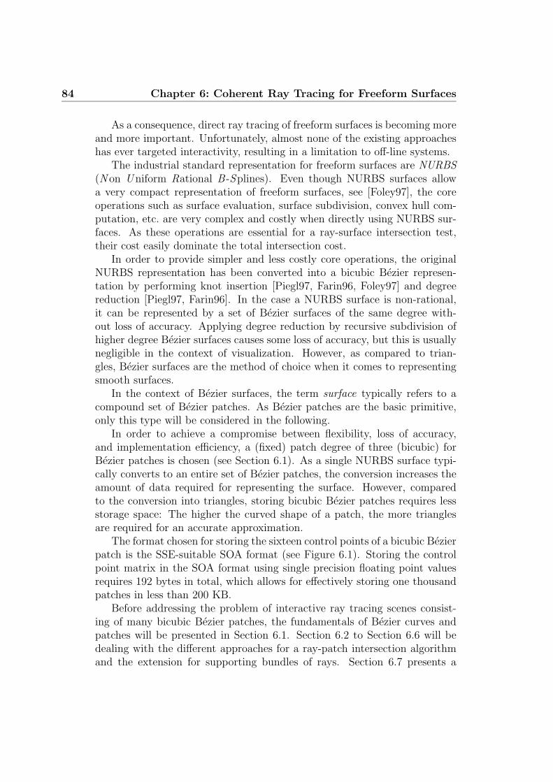
84 Chapter 6: Coherent Ray Tracing for Freeform Surfaces
As a consequence, direct ray tracing of freeform surfaces is becoming moreand more important. Unfortunately, almost none of the existing approacheshas ever targeted interactivity, resulting in a limitation to off-line systems.
The industrial standard representation for freeform surfaces are NURBS(N on Uniform Rational B -Splines). Even though NURBS surfaces allowa very compact representation of freeform surfaces, see [Foley97], the coreoperations such as surface evaluation, surface subdivision, convex hull com-putation, etc. are very complex and costly when directly using NURBS sur-faces. As these operations are essential for a ray-surface intersection test,their cost easily dominate the total intersection cost.
In order to provide simpler and less costly core operations, the originalNURBS representation has been converted into a bicubic Bezier represen-tation by performing knot insertion [Piegl97, Farin96, Foley97] and degreereduction [Piegl97, Farin96]. In the case a NURBS surface is non-rational,it can be represented by a set of Bezier surfaces of the same degree with-out loss of accuracy. Applying degree reduction by recursive subdivision ofhigher degree Bezier surfaces causes some loss of accuracy, but this is usuallynegligible in the context of visualization. However, as compared to trian-gles, Bezier surfaces are the method of choice when it comes to representingsmooth surfaces.
In the context of Bezier surfaces, the term surface typically refers to acompound set of Bezier patches. As Bezier patches are the basic primitive,only this type will be considered in the following.
In order to achieve a compromise between flexibility, loss of accuracy,and implementation efficiency, a (fixed) patch degree of three (bicubic) forBezier patches is chosen (see Section 6.1). As a single NURBS surface typi-cally converts to an entire set of Bezier patches, the conversion increases theamount of data required for representing the surface. However, comparedto the conversion into triangles, storing bicubic Bezier patches requires lessstorage space: The higher the curved shape of a patch, the more trianglesare required for an accurate approximation.
The format chosen for storing the sixteen control points of a bicubic Bezierpatch is the SSE-suitable SOA format (see Figure 6.1). Storing the controlpoint matrix in the SOA format using single precision floating point valuesrequires 192 bytes in total, which allows for effectively storing one thousandpatches in less than 200 KB.
Before addressing the problem of interactive ray tracing scenes consist-ing of many bicubic Bezier patches, the fundamentals of Bezier curves andpatches will be presented in Section 6.1. Section 6.2 to Section 6.6 will bedealing with the different approaches for a ray-patch intersection algorithmand the extension for supporting bundles of rays. Section 6.7 presents a
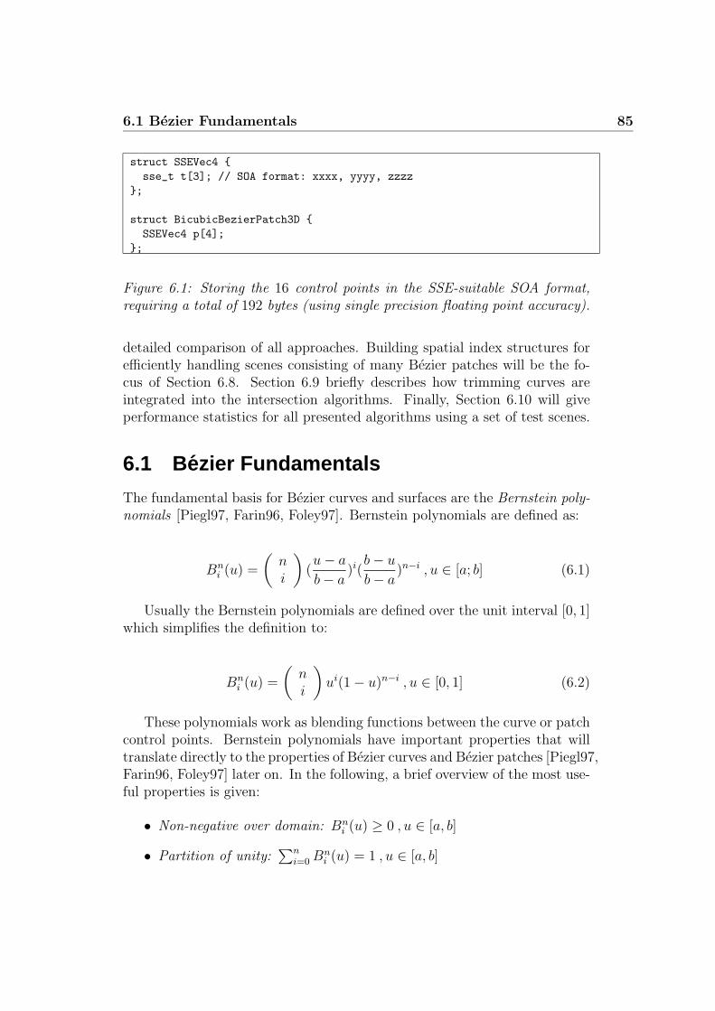
6.1 Bezier Fundamentals 85
struct SSEVec4 {
sse_t t[3]; // SOA format: xxxx, yyyy, zzzz
};
struct BicubicBezierPatch3D {
SSEVec4 p[4];
};
Figure 6.1: Storing the 16 control points in the SSE-suitable SOA format,requiring a total of 192 bytes (using single precision floating point accuracy).
detailed comparison of all approaches. Building spatial index structures forefficiently handling scenes consisting of many Bezier patches will be the fo-cus of Section 6.8. Section 6.9 briefly describes how trimming curves areintegrated into the intersection algorithms. Finally, Section 6.10 will giveperformance statistics for all presented algorithms using a set of test scenes.
6.1 Bezier Fundamentals
The fundamental basis for Bezier curves and surfaces are the Bernstein poly-nomials [Piegl97, Farin96, Foley97]. Bernstein polynomials are defined as:
Bni (u) =
(
ni
)
(u − a
b − a)i(
b − u
b − a)n−i , u ∈ [a; b] (6.1)
Usually the Bernstein polynomials are defined over the unit interval [0, 1]which simplifies the definition to:
Bni (u) =
(
ni
)
ui(1 − u)n−i , u ∈ [0, 1] (6.2)
These polynomials work as blending functions between the curve or patchcontrol points. Bernstein polynomials have important properties that willtranslate directly to the properties of Bezier curves and Bezier patches [Piegl97,Farin96, Foley97] later on. In the following, a brief overview of the most use-ful properties is given:
• Non-negative over domain: Bni (u) ≥ 0 , u ∈ [a, b]
• Partition of unity:∑n
i=0 Bni (u) = 1 , u ∈ [a, b]

86 Chapter 6: Coherent Ray Tracing for Freeform Surfaces
• Recursive definition: Bni (u) = ( b−u
b−a)Bn−1
i (u) + (u−ab−a
)Bn−1i−1 (u)
• Derivatives: (Bni (u))
′
= n(Bn−1i−1 (u) − Bn−1
i (u))
For example, the Bernstein polynomials of degree three are defined bythe following four equations:
B30(u) =
(
30
)
u0(1 − u)3 = (1 − u)3 (6.3)
B31(u) =
(
31
)
u1(1 − u)2 = 3u(1 − u)2
B32(u) =
(
32
)
u2(1 − u)1 = 3u2(1 − u)
B33(u) =
(
33
)
u3(1 − u)0 = u3
For efficiency reasons it is not advisable to evaluate these functions viatheir recursive definition, but to use the compact form of Equation 6.3.
6.1.1 Bezier Curves
Bezier curves of degree n are defined over a set of control points {Pi, 0 ≤ i ≤ n}which define the shape of the curve. The basis functions of Bezier curves arethe Bernstein polynomials, resulting in the following curve definition:
P n(u) =∑n
i=0 Bni (u)Pi , Pi ∈ R
n
The control points Pi are usually elements of R2 or R
3. A single bicu-bic Bezier curve (see Figure 6.2) can therefore be efficiently represented by4 ∗ 2 ∗ 4 = 32 bytes using single precision floating point values. The poly-gon defined by the control points is called control polygon.
As using Bernstein polynomials are used as the basis functions, Beziercurves inherit some useful properties:
• Convex Hull: The inherited properties of non-negativity (and the par-tition of unity) cause any point of the curve to be inside the convexhull of the curve control points.
• Interpolation of start and end point: The curve will pass through thestart and end points defining the curve, e.g. P n(0) = P0 and P n(1) =Pn.
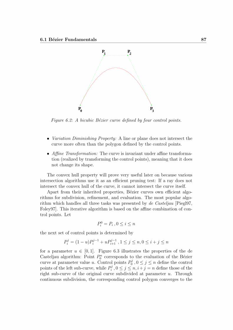
6.1 Bezier Fundamentals 87
P
PP
P0
1 2
3
Figure 6.2: A bicubic Bezier curve defined by four control points.
• Variation Diminishing Property: A line or plane does not intersect thecurve more often than the polygon defined by the control points.
• Affine Transformation: The curve is invariant under affine transforma-tion (realized by transforming the control points), meaning that it doesnot change its shape.
The convex hull property will prove very useful later on because variousintersection algorithms use it as an efficient pruning test: If a ray does notintersect the convex hull of the curve, it cannot intersect the curve itself.
Apart from their inherited properties, Bezier curves own efficient algo-rithms for subdivision, refinement, and evaluation. The most popular algo-rithm which handles all three tasks was presented by de Casteljau [Piegl97,Foley97]. This iterative algorithm is based on the affine combination of con-trol points. Let
P 0i = Pi , 0 ≤ i ≤ n
the next set of control points is determined by
P ji = (1 − u)P j−1
i + uP j−1i+1 , 1 ≤ j ≤ n, 0 ≤ i + j ≤ n
for a parameter u ∈ [0, 1]. Figure 6.3 illustrates the properties of the deCasteljau algorithm: Point P n
0 corresponds to the evaluation of the Beziercurve at parameter value u. Control points P j
0 , 0 ≤ j ≤ n define the controlpoints of the left sub-curve, while P j
i , 0 ≤ j ≤ n, i+ j = n define those of theright sub-curve of the original curve subdivided at parameter u. Throughcontinuous subdivision, the corresponding control polygon converges to the

88 Chapter 6: Coherent Ray Tracing for Freeform Surfaces
P 0
0
P 1
0
P 2
0
P 0
1P 0
2
P 2
1
P 1
2
P 0
3
P 1
1
P 3
0
P0
0P
0
1P
0
2P
0
3
P1
0P
1
1P
1
2
P2
1P
2
0
P3
0
u u u1−u 1−u 1−u
u 1−u u
1−u u
1−u
Figure 6.3: Left: Applying the de Casteljau algorithm for a bicubic Beziercurve P (u) with u = 0.5. P n
0 corresponds to point P (0.5). P j0 , 0 ≤ j ≤ 3
defines the control points of the left sub-curve, P ji , 0 ≤ j ≤ 3, i + j = 3 those
of the right sub-curve. Right: The de Casteljau algorithm illustrated as atriangular scheme of linear combinations.
curve itself and can therefore be used (following a sufficient number of subdi-visions) as an approximation. This process is often referred to as refinement.
6.1.2 Bezier Patches
A Bezier patch is a surface extension (tensor product) of a Bezier curve. Itis constructed from n × m control points {Pij, 0 ≤ i ≤ n, 0 ≤ j ≤ m} usingproducts of two univariate Bernstein polynomials as blending functions. ABezier patch is defined as a two-dimensional parametric function:
P (u, v) =∑n
i=0
∑m
j=0 Bni (u)Bm
j (v)Pij , Pij ∈ Rn
A bicubic Bezier patch (see Figure 6.4) with its 4× 4 = 16 control pointsdefined in R
3 can be efficiently represented by 16 ∗ 3 ∗ 4 = 192 bytes usingsingle precision accuracy.
Similar properties as for Bezier curves also hold for Bezier patches: P00,P0n, Pm0, Pnm are on the patch surface, the patch lies in the convex hull of itscontrol points, and the patch is invariant under affine transformation. Thede Casteljau algorithm for Bezier patches works similar to the one for Beziercurves, with the exception that the algorithm can be applied to either one ofthe two parametric directions (see Figure 6.3).
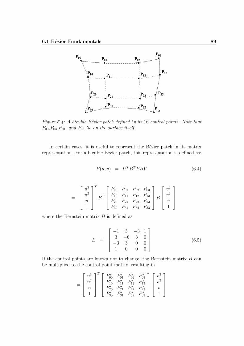
6.1 Bezier Fundamentals 89
01
03
10
0002
P P PP
P12P 13P
2220 PP
30P 3233
P P
23P
11P
31P
P21
Figure 6.4: A bicubic Bezier patch defined by its 16 control points. Note thatP00,P03,P30, and P33 lie on the surface itself.
In certain cases, it is useful to represent the Bezier patch in its matrixrepresentation. For a bicubic Bezier patch, this representation is defined as:
P (u, v) = UT BT PBV (6.4)
=
u3
u2
u1
T
BT
P00 P01 P02 P03
P10 P11 P12 P13
P20 P21 P22 P23
P30 P31 P32 P33
B
v3
v2
v1
where the Bernstein matrix B is defined as
B =
−1 3 −3 13 −6 3 0−3 3 0 01 0 0 0
(6.5)
If the control points are known not to change, the Bernstein matrix B canbe multiplied to the control point matrix, resulting in
=
u3
u2
u1
T
P ∗
00 P ∗
01 P ∗
02 P ∗
03
P ∗
10 P ∗
11 P ∗
12 P ∗
13
P ∗
20 P ∗
21 P ∗
22 P ∗
23
P ∗
30 P ∗
31 P ∗
32 P ∗
33
v3
v2
v1

90 Chapter 6: Coherent Ray Tracing for Freeform Surfaces
The evaluation of P (u, v) through the application of the new matrix P ∗
ij
requires only multiplication (from left and right) with the two vectors UT
and V . This allows for a more efficient implementation. In the same manner,the derivatives can be determined by simply replacing the vector UT byU
′T =[
3u2 2u 1 0]
, respectively V by V′
.
6.2 The Ray-Patch Intersection Problem
Testing for a valid intersection between a ray and a bicubic Bezier patchis a significantly more complex operation than a ray-triangle intersectiontest. In the last two decades researchers have proposed many approachesfor solving the intersection problem. In the following, some of these will bebriefly discussed.
Nishita et al. [Nishita90] described an iterative algorithm called Bezierclipping (see Section 6.6) to compute ray-patch intersections by identifyingand cutting away regions of the patch, which are known not to intersect theray. Campagna et al. [Campagna97] later solved inherent numerical issues ofthe original algorithm and proposed algorithmic optimizations.
Martin et al. [Martin00] presented a framework for integrating ray tracingof trimmed NURBS into existing rendering architectures. The frameworkcan be easily transferred for handling bicubic Bezier patches instead of theoriginal NURBS. A numerical approach called Newton iteration was chosen asbasis for intersection computation. Newton iteration (see Section 6.4) allowsfor quickly converging to a solution if the starting values are sufficiently closeto the correct solution. Martin et al. used a spatial subdivision structure foreach patch to ensure a sufficiently close starting values.
Wang et al. [Wang01] combined Newton iteration with Bezier clippingand used the coherence of neighboring rays to speed up Nishita’s originalalgorithm by roughly a factor of three. Unfortunately, the algorithm requiresadditional data structures to prevent wrong results through reusing the dataof neighboring rays.
Sweeney et al. [Sweeney86] concentrated on speeding up ray tracing ofB-Spline surfaces by basing the initial guess of the Newton iteration on theintersection between a ray and the sufficiently refined control mesh.
Researchers have also proposed dedicated hardware designs for ray tracingfreeform surfaces. Lewis et al. [Lewis02] presented a design of a pipelinedarchitecture for ray-patch intersection. The design is too closely related tocustom hardware to be beneficial for a software approach. Furthermore, itsmain target was to serve as a proof of concept, and not to provide a highperformance solution.
6.3 Uniform Refinement 91
Parker et al. [Parker99b] implemented a realtime ray tracing system usinga massively parallel approach (a large shared-memory supercomputer). Thesystem also supported Bezier patches, while using Newton iteration for ray-patch intersection.
To sum it up, all approaches so far more or less have been focused on ageneral implementation and have never explicitly targeted high performance.Furthermore, the corresponding algorithms were neither designed nor imple-mented with respect to the underlying processor architecture, causing majorperformance penalties.
Approaches designed exclusively to the underlying hardware have beenproposed by Benthin et al. [Benthin04] and Geimer et al. [Geimer05]. Bothmethods have been optimized to achieve interactive performance on a singleCPU (see Section 6.3 and Section 6.4).
In the following, intersection algorithms considered suitable for fast im-plementation will be discussed in detail. Bottlenecks, performance issuesand, in particular, coding guidelines for an implementation using SSE in-structions will be presented. Moreover, it will be shown that, depending onthe algorithm, the approach of performing intersection computation for abundle of rays in parallel (see Chapter 5) is also beneficial in the context ofbicubic Bezier patches.
6.3 Uniform Refinement
As a basis for the first ray-patch intersection algorithm, a simple refinement-based approach is chosen. Refinement allows for easily controlling approxi-mation accuracy and, in particular, isolating the spatial location of the inter-section. The refinement-based intersection thus relies on the following coreoperations:
Pruning: A conservative and simple pruning test is used to decide whetherthe ray can intersect a given patch or not.
Refinement: A refinement step subdivides a given patch into a set of (usu-ally two to four) child patches.
Final Intersection: When reaching the maximum refinement level, an in-tersection test with an approximate representation of the current patchis performed.
Instead of adaptively refining the patch, a maximum predefined refine-ment level is used. It may seem that introducing the additional work of

92 Chapter 6: Coherent Ray Tracing for Freeform Surfaces
BicubicBezierPatch3D patch; // current active patch
Stack stack; // patch stack
int depth = 0;
while(1)
{
while(1)
{
if (Prune(patch)) break;
if (depth == MAX_DEPTH)
{
FinalIntersection(patch);
break;
}
if (depth % 2)
patch.RefineHorizontal(child0,child1);
else
patch.RefineVertical(child0,child1);
depth++;
patch = child0;
stack.push(child1,depth);
}
if (stack.empty()) break;
stack.pop(patch,depth);
}
Figure 6.5: Pseudo C++ code for intersection based on three core opera-tions for uniform refinement. The parametric direction for the refinementoperation is determined by the current refinement depth.
refining the patch to a fixed predefined level is not as clever as avoidingthe work by adaptive refining, but it makes the previously required crack-handling and adaptivity tests obsolete. The main difficulty of this approachis to chose the right refinement level, see [Benthin04].
Figure 6.5 shows an example implementation for the complete ray-patchintersection step. Note that uniform refinement does not require additionaldata structures. This makes the algorithm very memory-efficient. In thefollowing, the core operations will be discussed in detail.
6.3.1 Pruning Implementation
The pruning operation can be seen as the most important of all core op-erations, because it is the first one in order and therefore the one appliedmost often (a pruned patch is never refined nor intersected). To efficientlyimplement the pruning operation we represent the ray as the intersection of

6.3 Uniform Refinement 93
inline bool Prune(const BicubicBezierPatch3D &patch,
const RayPlanesSSE &plane)
{
unsigned int signsU = 0;
for (unsigned int i=0;i<4;i++)
{
const sse_t d = _mm_add_ps(_mm_add_ps(_mm_mul_ps(plane.Nu.t[0],
patch.p[i].t[0]),
_mm_mul_ps(plane.Nu.t[1],
patch.p[i].t[1])),
_mm_mul_ps(plane.Nu.t[2],patch.p[i].t[2]));
signsU |= _mm_movemask_ps(_mm_sub_ps(d,plane.du)) << (4*i);
}
if (signsU == 0xffff || signsU == 0) return true;
unsigned int signsV = 0;
for (unsigned int i=0;i<4;i++)
{
const sse_t d = _mm_add_ps(_mm_add_ps(_mm_mul_ps(plane.Nv.t[0],
patch.p[i].t[0]),
_mm_mul_ps(plane.Nv.t[1],
patch.p[i].t[1])),
_mm_mul_ps(plane.Nv.t[2],patch.p[i].t[2]));
signsV |= _mm_movemask_ps(_mm_sub_ps(d,plane.dv)) << (4*i);
}
if (signsV == 0xffff || signsV == 0) return true;
return false;
}
Figure 6.6: Fast pruning test by testing the signs of control point distances tothe two ray planes. If the sixteen signs match, all control points lie entirelyin one half-space determined by one of the ray planes, and the correspondingpatch cannot be intersected by the ray.
two orthogonal planes [Sweeney86, Woodward89]. The distance of all con-trol points to both planes are computed yielding 2D coordinates. If all 2Dcoordinates lie entirely in one half-space (with respect to a certain plane),the ray cannot intersect the corresponding patch because of the convex hullcriteria.
The projection of control points can be realized via a sequence of dotproducts. SSE instructions allow for performing four dot product operationsin parallel. For the entire patch, this results in only 12 parallel multiplicationsand 12 parallel additions plus 1 instruction for obtaining the sign bits for eachplane (see Figure 6.6).

94 Chapter 6: Coherent Ray Tracing for Freeform Surfaces
inline void RefineVertical(BicubicBezierPatch3D &patch0,
BicubicBezierPatch3D &patch1)
{
static const sse_t half = _mm_set_ps1(0.5f);
patch0.p[0] = p[0];
patch1.p[3] = p[3];
patch0.p[1].t[0] = _mm_mul_ps(half,_mm_add_ps(p[0].t[0],p[1].t[0]));
patch0.p[1].t[1] = _mm_mul_ps(half,_mm_add_ps(p[0].t[1],p[1].t[1]));
patch0.p[1].t[2] = _mm_mul_ps(half,_mm_add_ps(p[0].t[2],p[1].t[2]));
patch1.p[2].t[0] = _mm_mul_ps(half,_mm_add_ps(p[2].t[0],p[3].t[0]));
patch1.p[2].t[1] = _mm_mul_ps(half,_mm_add_ps(p[2].t[1],p[3].t[1]));
patch1.p[2].t[2] = _mm_mul_ps(half,_mm_add_ps(p[2].t[2],p[3].t[2]));
const sse_t p11x = _mm_mul_ps(half,_mm_add_ps(p[1].t[0],p[2].t[0]));
patch0.p[2].t[0] = _mm_mul_ps(half,_mm_add_ps(patch0.p[1].t[0],p11x));
patch1.p[1].t[0] = _mm_mul_ps(half,_mm_add_ps(patch1.p[2].t[0],p11x));
const sse_t p11y = _mm_mul_ps(half,_mm_add_ps(p[1].t[1],p[2].t[1]));
patch0.p[2].t[1] = _mm_mul_ps(half,_mm_add_ps(patch0.p[1].t[1],p11y));
patch1.p[1].t[1] = _mm_mul_ps(half,_mm_add_ps(patch1.p[2].t[1],p11y));
const sse_t p11z = _mm_mul_ps(half,_mm_add_ps(p[1].t[2],p[2].t[2]));
patch0.p[2].t[2] = _mm_mul_ps(half,_mm_add_ps(patch0.p[1].t[2],p11z));
patch1.p[1].t[2] = _mm_mul_ps(half,_mm_add_ps(patch1.p[2].t[2],p11z));
const sse_t p30x = _mm_mul_ps(half,_mm_add_ps(patch0.p[2].t[0],
patch1.p[1].t[0]));
patch0.p[3].t[0] = p30x;
patch1.p[0].t[0] = p30x;
const sse_t p30y = _mm_mul_ps(half,_mm_add_ps(patch0.p[2].t[1],
patch1.p[1].t[1]));
patch0.p[3].t[1] = p30y;
patch1.p[0].t[1] = p30y;
const sse_t p30z = _mm_mul_ps(half,_mm_add_ps(patch0.p[2].t[2],
patch1.p[1].t[2]));
patch0.p[3].t[2] = p30z;
patch1.p[0].t[2] = p30z;
}
Figure 6.7: Vertical patch refinement by applying the de Casteljau algorithm.The original patch is subdivided into two sub-patches. Note that the algorithmonly relies on multiply-add sequences.
6.3.2 Refinement Implementation
The refinement operation itself is based on the de Casteljau algorithm [Foley97],which splits the patch in half along a chosen parametric direction (either ’v’or ’u’) producing two refined child patches. Alternating the parametric di-rection at each refinement level ensures uniform refinement.
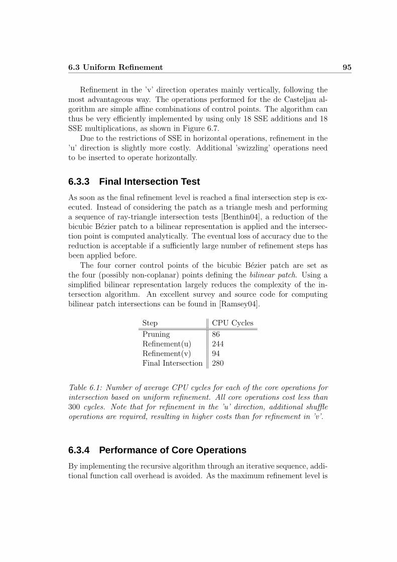
6.3 Uniform Refinement 95
Refinement in the ’v’ direction operates mainly vertically, following themost advantageous way. The operations performed for the de Casteljau al-gorithm are simple affine combinations of control points. The algorithm canthus be very efficiently implemented by using only 18 SSE additions and 18SSE multiplications, as shown in Figure 6.7.
Due to the restrictions of SSE in horizontal operations, refinement in the’u’ direction is slightly more costly. Additional ’swizzling’ operations needto be inserted to operate horizontally.
6.3.3 Final Intersection Test
As soon as the final refinement level is reached a final intersection step is ex-ecuted. Instead of considering the patch as a triangle mesh and performinga sequence of ray-triangle intersection tests [Benthin04], a reduction of thebicubic Bezier patch to a bilinear representation is applied and the intersec-tion point is computed analytically. The eventual loss of accuracy due to thereduction is acceptable if a sufficiently large number of refinement steps hasbeen applied before.
The four corner control points of the bicubic Bezier patch are set asthe four (possibly non-coplanar) points defining the bilinear patch. Using asimplified bilinear representation largely reduces the complexity of the in-tersection algorithm. An excellent survey and source code for computingbilinear patch intersections can be found in [Ramsey04].
Step CPU Cycles
Pruning 86Refinement(u) 244Refinement(v) 94Final Intersection 280
Table 6.1: Number of average CPU cycles for each of the core operations forintersection based on uniform refinement. All core operations cost less than300 cycles. Note that for refinement in the ’u’ direction, additional shuffleoperations are required, resulting in higher costs than for refinement in ’v’.
6.3.4 Performance of Core Operations
By implementing the recursive algorithm through an iterative sequence, addi-tional function call overhead is avoided. As the maximum refinement level is
96 Chapter 6: Coherent Ray Tracing for Freeform Surfaces
known in advance, the memory for storing refined patches is constant and cantherefore be allocated in advance (avoiding costly memory allocation calls).As an example, the ray-patch intersection code reserves 32 ∗ 192 = 6144bytes for a maximum refinement level of 32.
Table 6.1 shows with careful optimization, almost all core operations canbe executed in less than 300 cycles (measured using the internal CPU clockcycle counter). Note that the current implementation still leaves room foroptimization, allowing for even faster execution.
6.3.5 Extension for Ray Bundles
The uniform refinement approach is especially suitable for tracing ray bundlesbecause the refinement operations are independent of the number of rayswithin a bundle. This allows for efficiently amortizing the cost of refinementover the rays within the bundle. Nevertheless, the other core operations fortracing bundles need to be adjusted accordingly.
Pruning for ray bundles has to be adapted in the following way: If evenone ray in the bundle indicates an intersection of a patch, it must not bepruned. As long as coherence within the ray bundle is high enough almostall rays will produce the same decision in the pruning step.
As long as all rays can be grouped within a coherent beam (e.g. for pri-mary rays), the pruning test can be simplified further. By constructing fourplanes out of the four corner rays spanning the beam one can easily decide(distance to plane) if all control points are outside the beam or not. Usingthis technique, the number of required plane tests can be significantly re-duced. Instead of constructing two planes for each ray, only four planes forthe entire bundle are needed. The complete pruning operation based on thefour corner rays has an average cost of 240 cycles per 16-ray bundle, corre-sponding to an average of only 15 cycles per ray. The code in Figure 6.6 canbe easily adapted to test against four instead of two planes.
The final intersection step must be applied for all rays within a bundleand cannot be easily amortized. It therefore turns out that this step is verytime-critical. As SSE operates on four data elements at once it is mostbeneficial to perform the final intersection in bundles of four rays. Bilinearpatch intersection as presented in [Ramsey04] can be coded easily using SSEfor four rays in parallel. This parallel bilinear intersection code is able toreduce the average cost per ray for the final intersection step from 280 toonly 88 cycles.

6.4 Newton Iteration 97
6.4 Newton Iteration
Newton iteration is a common technique for solving equations of the formf(x) = 0. It approximates the roots of function f(x) by using the first termsof the Taylor series for f(x). The Taylor series of f(x) regarding pointx = x0 + ε is defined as
f(x0 + ε) = f(x0) + f′
(x0)ε +1
2f
′′
(x0)ε2 + ... (6.6)
A restriction to only the first derivative results in
f(x0 + ε) ≈ f(x0) + f′
(x0)ε (6.7)
By starting from an initial guess x0, Equation 6.7 can be used to determinethe value for ε by setting ε0 = ε
ε0 = −f(x0)
f ′(x0)(6.8)
The resulting ε0 can be seen as the offset to the root’s position. Throughcontinuous adjustment of
εn = −f(xn)
f ′(xn)(6.9)
an iterative sequence
xn+1 = xn −f(xn)
f ′(xn)(6.10)
is defined. The sequence converges to the root if the starting value x0 issufficiently close to this value. The need to chose a sufficiently close startingvalue is at the same time a major disadvantage of this method because of theinstability near a horizontal asymptote or a local extremum. If the Newtoniteration converges, it does so quadratically, which intuitively means that thenumber of correct digits of the root approximation roughly doubles in everystep.
In the following sections, techniques for applying the Newton iteration inorder to solve the ray-patch intersection problem will be discussed. Sec-tion 6.4.1 will illustrate the algorithm itself, while Section 6.4.2 to Sec-tion 6.4.4 will provide guidelines for an SSE implementation and will discussan extension for supporting ray bundles. Section 6.4.5 will present resultsand will discuss limitations and bottlenecks.

98 Chapter 6: Coherent Ray Tracing for Freeform Surfaces
6.4.1 Newton Iteration Algorithm
As shown by Martin et al. [Martin00], the Newton iteration represents anefficient framework for handling the ray-patch intersection problem. Startingfrom two perpendicular planes
P0 := (N0, d0) N0 x + d0 = 0
P1 := (N1, d1) N1 x + d1 = 0 Ni ∈ R3, di ∈ R
whose intersection represents the ray, the aim is to find the roots for thefollowing function
F (u, v) =
(
N0 P (u, v) + d0
N1 P (u, v) + d1
)
(6.11)
The Newton iteration for this case looks as follows
(
un+1
vn+1
)
=
(
un
vn
)
− P (un, vn) J−1(un, vn) (6.12)
The term J is the Jacobian matrix
J =
(
N0∂∂u
P (u, v) N0∂∂v
P (u, v)N1
∂∂u
P (u, v) N1∂∂v
P (u, v)
)
(6.13)
where J−1 is defined as
J−1 =adj(J)
det(J)(6.14)
As J is a 2 × 2 matrix, the adjoint of J is
adj(J) =
(
J22 −J12
−J21 J11
)
(6.15)
The Newton iteration stops as soon as
||P (un, vn)|| < ε , (6.16)
where ||P (u, v)|| defines the distance of P (u, v) to the ray (more precisely, tothe two ray planes) and ε is defined as an accuracy threshold. As an earlyexit point, Martin et al. [Martin00] suggested the following condition:
6.4 Newton Iteration 99
||P (un+1, vn+1)|| > ||P (un, vn)|| (6.17)
If for the current iteration the distance to the ray is greater than the dis-tance of the previous iteration, an early exit is performed. Additionally,the iteration stops if the number of iterations is greater than a predefinedthreshold.
If the Newton iteration returns a valid solution (u∗, v∗), the distance of thecorresponding intersection point needs to be compared with the ray origin.P (u, v) is therefore evaluated at the parameter values (u∗, v∗) in order toobtain the intersection point. By projecting the intersection point along theray direction, the distance t can be computed as
t = ray.direction ∗ (P (u, v) − ray.origin) (6.18)
Equations 6.13 and 6.16 demonstrate that the actual implementation requiresonly two core operations:
• Evaluation of the partial derivatives ∂∂u
P (u, v) and ∂∂v
P (u, v).
• Evaluation of P (u, v).
As evaluating P (u, v) is very similar to the evaluation of ∂∂u
P (u, v), thefocus will be on optimizing a code sequence which handles both cases (seeSection 6.4.2).
Additionally, the Newton iteration algorithm allows for performing theintersection computation for multiple rays in parallel, which is beneficial forhandling ray bundles. As with triangle intersection (see Chapter 5), it isbeneficial to perform the intersection for patches for four rays in parallel (seeSection 6.4.2).
6.4.2 SSE Implementation
Geimer et al. [Geimer05] showed that the evaluation of P (u, v) and the par-tial derivatives can be efficiently performed by computing a vector-matrix-vector product. The modified control point matrix P ∗
ij of Section 6.1.2 avoidsthe required evaluation of the Bernstein basis functions (see Equation 6.4).Therefore, P (u, v) can be evaluated by the following vector-matrix-vectorproduct:

100 Chapter 6: Coherent Ray Tracing for Freeform Surfaces
inline R3 Evaluate(const BicubicBezierPatch3D &patch,
const float u,
const float v)
{
const sse_t V = _mm_setr_ps(v*v*v,v*v,v,1.0f);
const sse_t u2 = _mm_set_ps1(u);
const sse_t u1 = _mm_mul_ps(u2,u2);
const sse_t u0 = _mm_mul_ps(u1,u2);
const sse_t X = _mm_add_ps(_mm_add_ps(_mm_mul_ps(patch.p[0].t[0],u0),
_mm_mul_ps(patch.p[1].t[0],u1)),
_mm_add_ps(_mm_mul_ps(patch.p[2].t[0],u2),
patch.p[3].t[0]));
const float x = _mm_cvtss_f32(sseHorizontalAdd(_mm_mul_ps(X,V)));
const sse_t Y = _mm_add_ps(_mm_add_ps(_mm_mul_ps(patch.p[0].t[1],u0),
_mm_mul_ps(patch.p[1].t[1],u1)),
_mm_add_ps(_mm_mul_ps(patch.p[2].t[1],u2),
patch.p[3].t[1]));
const float y = _mm_cvtss_f32(sseHorizontalAdd(_mm_mul_ps(Y,V)));
const sse_t Z = _mm_add_ps(_mm_add_ps(_mm_mul_ps(patch.p[0].t[2],u0),
_mm_mul_ps(patch.p[1].t[2],u1)),
_mm_add_ps(_mm_mul_ps(patch.p[2].t[2],u2),
patch.p[3].t[2]));
const float z = _mm_cvtss_f32(sseHorizontalAdd(_mm_mul_ps(Z,V)));
return R3(x,y,z);
}
Figure 6.8: Evaluating P (u, v) by performing a vector-matrix-vector productby SSE instructions. Through the SOA layout, horizontal operations arerequired to compute the sum of all register elements.
P (u, v) =
u3
u2
u1
T
P ∗
00 P ∗
01 P ∗
02 P ∗
03
P ∗
10 P ∗
11 P ∗
12 P ∗
13
P ∗
20 P ∗
21 P ∗
22 P ∗
23
P ∗
30 P ∗
31 P ∗
32 P ∗
33
v3
v2
v1
(6.19)
Additionally, the evaluation of P (u, v) can be efficiently implemented usingSSE instructions. The implementation shown in Figure 6.8 starts with u andv as float values. Shuffle operations are required to copy float values into allregister elements. Moreover, adding elements horizontally within a registerrequires additional operations.

6.4 Newton Iteration 101
Computing the derivatives in the same way allows for reducing the num-ber of instructions because components which are multiplied by zero arenot considered any further. Table 6.2 shows the average number of cyclesfor three different core operations. Even though almost all core operationsrequire less than 100 cycles, the cost could be further reduced as soon asprocessor architectures offer better support for horizontal and shuffle opera-tions.
Step Cycles
Evaluate 90Derivative(u) 90Derivative(v) 79
Table 6.2: Average number of CPU cycles for each of the core operations(single ray). All core operations require less than 100 cycles. For the deriva-tive in the ’u’ direction, fewer shuffle operations are required, resulting inlower costs than for the derivative in ’v’.
6.4.3 Extension for Ray Bundles
Adapting the intersection for ray bundles is straightforward. As SSE allowsfor operating on four data elements using a single instruction, it is beneficialto apply the Newton iteration for bundles of four rays in parallel. Performingfour Newton iterations in parallel makes it necessary to evaluate P (u, v)for two vectors U = (u0, u1, u2, u3) and V = (v0, v1, v2, v3) in parallel (seeFigure 6.9). Even though the layout of U and V avoids additional horizontaloperations (such as required for the single ray implementation), the four-rayimplementation requires that every control point coordinate be copied intothe four register elements by an additional shuffle instruction.
One could avoid the shuffle instruction by storing every control point co-ordinate as an SSE data type, but this would increase the patch data storagecosts by a factor of 4, thus significantly affecting the advantage of compactdata representation. On the other hand, one could use larger bundles (ofmore than four rays) to amortize the cost for the shuffle instruction, but thelimited number of registers makes this approach inefficient.
Table 6.3 shows the average number of required CPU cycles. On a perray basis, the costs for the core operations are reduced, in particular forevaluating the derivatives.

102 Chapter 6: Coherent Ray Tracing for Freeform Surfaces
inline void Evaluate4(const sse_t u,
const sse_t v,
const BicubicBezierPatch3D &patch,
SSEVec4 &result)
{
const sse_t u2 = u;
const sse_t u1 = _mm_mul_ps(u,u);
const sse_t u0 = _mm_mul_ps(u,u1);
const sse_t v2 = v;
const sse_t v1 = _mm_mul_ps(v,v);
const sse_t v0 = _mm_mul_ps(v,v1);
// == X ==
const sse_t t0 = patch.p[0].t[0];
const sse_t t1 = patch.p[1].t[0];
const sse_t t2 = patch.p[2].t[0];
const sse_t t3 = patch.p[3].t[0];
const sse_t x0 = _mm_add_ps(_mm_add_ps(_mm_mul_ps(SHUFFLE(t0,0),u0),
_mm_mul_ps(SHUFFLE(t1,0),u1)),
_mm_add_ps(_mm_mul_ps(SHUFFLE(t2,0),u2),
SHUFFLE(t3,0)));
const sse_t x1 = _mm_add_ps(_mm_add_ps(_mm_mul_ps(SHUFFLE(t0,1),u0),
_mm_mul_ps(SHUFFLE(t1,1),u1)),
_mm_add_ps(_mm_mul_ps(SHUFFLE(t2,1),u2),
SHUFFLE(t3,1)));
const sse_t x2 = _mm_add_ps(_mm_add_ps(_mm_mul_ps(SHUFFLE(t0,2),u0),
_mm_mul_ps(SHUFFLE(t1,2),u1)),
_mm_add_ps(_mm_mul_ps(SHUFFLE(t2,2),u2),
SHUFFLE(t3,2)));
const sse_t x3 = _mm_add_ps(_mm_add_ps(_mm_mul_ps(SHUFFLE(t0,3),u0),
_mm_mul_ps(SHUFFLE(t1,3),u1)),
_mm_add_ps(_mm_mul_ps(SHUFFLE(t2,3),u2),
SHUFFLE(t3,3)));
result.t[0] = _mm_add_ps(_mm_add_ps(_mm_mul_ps(x0,v0),
_mm_mul_ps(x1,v1)),
_mm_add_ps(_mm_mul_ps(x2,v2),
x3));
// == Y,Z similar ==
// ..
}
Figure 6.9: Evaluating P (U, V ) for two vectors U = (u0, u1, u2, u3) andV = (v0, v1, v2, v3) by performing a vector-matrix-vector product using SSEinstructions. No horizontal operations are required but many shuffle instruc-tions, because each control point coordinate has to be copied into the fourregister elements.

6.4 Newton Iteration 103
Step Cycles / Per Four-Ray Bundle Cycles / Per Ray
Evaluate 350 87.5Derivative(u) 255 63.75Derivative(v) 244 61
Table 6.3: Average number of CPU cycles for each of the core operationswhen operating on four rays in parallel. Computing derivatives requires feweroperations, resulting in lower costs.
6.4.4 Newton Iteration Convergence
The greatest difficulty by the Newton iteration is the fact that convergencedepends on the starting value. If the starting point is chosen too far awayfrom the correct solution, the Newton iteration can converge to a wrongsolution (get “stuck” in a local minimum), converge slowly, or even fail toconverge at all.
In order to obtain a good starting value, researchers [Martin00] havesuggested to subdivide a given patch into a set of sub-patches (based on aflatness criteria [Guthe02]) and to build a spatial index structure from thesesub-patches. Each sub-patch corresponds to a specific parametric domainof the original patch. A ray, or a ray bundle, is then traversed through thisspatial index structure and, in the case of sub-patch intersection, the startingvalue of the Newton iteration is initialized to the center of the correspondingparametric domain of the sub-patch.
If the patch is sufficiently flat, patch subdivision for initializing startingvalues works quite well. Nevertheless, it can never guarantee convergence.Note that the creation of sub-patches typically requires a chosen flatness orcurvature threshold, which has to be manually adjusted depending on thecurvature of patches.
6.4.5 Discussion
The convergence speed of a Newton iteration-based intersection algorithm de-pends mainly on the distance between the starting value and the final result.If the distance is sufficiently small, Newton iteration offers quadratic conver-gence, which makes it extremely fast. Nevertheless, the standard approach ofdetermining a sufficiently close starting value by traversing an additional spa-tial index structure (see Section 6.4.4), which is constructed per patch, hasserious drawbacks. First of all, the overall memory requirements are higherbecause of the additional spatial structure per patch, making rendering of

104 Chapter 6: Coherent Ray Tracing for Freeform Surfaces
highly complex scenes difficult. Furthermore, the larger memory footprint in-creases the probability of cache misses. Finally, even a finely resolved spatialindex structure does not guarantee convergence in all potential cases.
The main advantage of a Newton iteration-based approach is that the ray-patch intersection costs essentially depend on the costs for evaluating P (U, V )and the corresponding derivatives. A closer look at the code itself shows thatthe evaluation almost exclusively consists of multiply-add sequences. This issimilar to the implementation of core operations for uniform refinement. Andhere too, the performance could be significantly increased using an exclusivemultiply-add SSE instruction and more SSE registers for storing temporaryvalues.
6.5 Newton Iteration and Krawczyk Operator
As discussed in Section 6.4, a Newton iteration-based algorithm can fail toconverge if the starting point is chosen too far away from the correct solution.Fortunately, the Krawczyk operator [Krawczyk69, Krawczyk70] is able todetermine for a chosen starting point if the Newton iteration will convergeor not. Therefore, the Krawczyk operator can be used as an extension to thestandard Newton iteration-based intersection in order to identify safe startingregions. The implementation described in this section is an extension of theoriginal work by Toth et al. [Toth85].
Before explaining the Krawczyk operator and the extension of the Newtoniteration-based intersection in detail, the fundamentals of interval arithmetic,which form the basis of a Krawczyk operator, are presented first.
6.5.1 Interval Arithmetic
An interval (over R) is defined as a bounded set of real numbers X =[Xmin, Xmax] = {x ∈ R : Xmin ≤ x ≤ Xmax}. For intervals, which in the fol-lowing will be indicated in capital letters, the standard arithmetic operations{+,−, ∗, /} are defined as:
X + Y = [Xmin + Ymin, Xmax + Ymax] (6.20)
X − Y = [Xmin − Ymax, Xmax − Ymin] (6.21)
X ∗ Y = [minx∗y,maxx∗y] (6.22)
1.0/X = [1.0/Xmax, 1.0/Xmin], 0 /∈ X (6.23)
When multiplying two intervals, the upper, respectively lower bound of theresult is computed by determining the maximum resp. minimum of the four
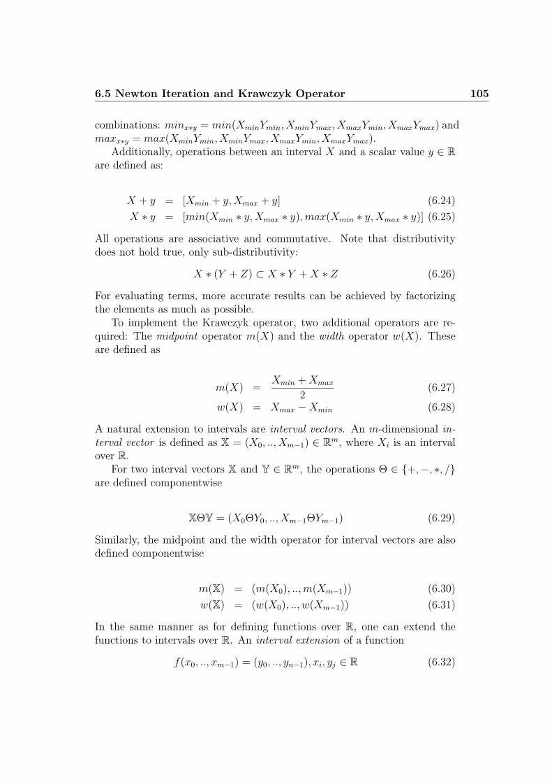
6.5 Newton Iteration and Krawczyk Operator 105
combinations: minx∗y = min(XminYmin, XminYmax, XmaxYmin, XmaxYmax) andmaxx∗y = max(XminYmin, XminYmax, XmaxYmin, XmaxYmax).
Additionally, operations between an interval X and a scalar value y ∈ R
are defined as:
X + y = [Xmin + y,Xmax + y] (6.24)
X ∗ y = [min(Xmin ∗ y,Xmax ∗ y),max(Xmin ∗ y,Xmax ∗ y)] (6.25)
All operations are associative and commutative. Note that distributivitydoes not hold true, only sub-distributivity:
X ∗ (Y + Z) ⊂ X ∗ Y + X ∗ Z (6.26)
For evaluating terms, more accurate results can be achieved by factorizingthe elements as much as possible.
To implement the Krawczyk operator, two additional operators are re-quired: The midpoint operator m(X) and the width operator w(X). Theseare defined as
m(X) =Xmin + Xmax
2(6.27)
w(X) = Xmax − Xmin (6.28)
A natural extension to intervals are interval vectors. An m-dimensional in-terval vector is defined as X = (X0, .., Xm−1) ∈ R
m, where Xi is an intervalover R.
For two interval vectors X and Y ∈ Rm, the operations Θ ∈ {+,−, ∗, /}
are defined componentwise
XΘY = (X0ΘY0, .., Xm−1ΘYm−1) (6.29)
Similarly, the midpoint and the width operator for interval vectors are alsodefined componentwise
m(X) = (m(X0), ..,m(Xm−1)) (6.30)
w(X) = (w(X0), .., w(Xm−1)) (6.31)
In the same manner as for defining functions over R, one can extend thefunctions to intervals over R. An interval extension of a function
f(x0, .., xm−1) = (y0, .., yn−1), xi, yj ∈ R (6.32)

106 Chapter 6: Coherent Ray Tracing for Freeform Surfaces
is defined as
F (X0, .., Xm−1) = (Y0, .., Yn−1) (6.33)
where Xi, Yj are intervals over R.
6.5.2 Krawczyk Operator
The Krawczyk operator K(Xi, y, Y ) is defined as:
K(Xi, y, Y ) = y − Y ∗ f(y) + (|Y | ∗ A ∗ e ∗ [−1, 1]) (6.34)
y = m(Xi) (6.35)
Y = m(F ′(Xi))−1 (6.36)
Aij =1
2(w(F ′(Xi)))ij (6.37)
ei =1
2(w(Xi))i (6.38)
where Xi is an interval extension of xi ∈ R, y ∈ Xi, and Y a non-singularmatrix. Without loss of generality, y = m(Xi) and Y = m(F ′(Xi))
−1. Thefundamental idea of applying the Krawczyk operator is to determine safeconvergence regions within interval Xi.
From the given interval Xi, the Krawczyk operator K(Xi, y, Y ) computesa new interval X
′
i . Based on the new interval X′
i , a convergence criteria isevaluated that determines if Xi can be considered as a safe region for startinga Newton iteration.
For a detailed description of the mathematical background, see [Krawczyk69,Krawczyk70, Toth85].
6.5.3 Krawczyk-Moore Intersection Algorithm
Based on the work by Moore [Moore77], Toth [Toth85] proposed an algo-rithm that uses the Krawczyk operator to identify safe regions for the New-ton iteration. If a solution for function f(x) = 0 with x ∈ X0 exists, theKrawczyk-Moore test will return an interval Xsafe for which all x ∈ Xsafe
converge to a non-ambiguous solution. The underlying process can be for-mulated as an iterative algorithm starting with the initial interval X0. Theintervals Xi builds a sequence of nested intervals:

6.5 Newton Iteration and Krawczyk Operator 107
X1 = X0
⋂
K(X0,m(X0),m(F ′(X0))−1) (6.39)
X2 = X1
⋂
K(X1,m(X1),m(F ′(X1))−1) (6.40)
... (6.41)
Xi+1 = Xi
⋂
K(Xi,m(Xi),m(F ′(Xi))−1) (6.42)
The sequence can be terminated if one of the follow conditions holds true:
• Xi is a safe region for starting the Newton iteration
• Xi = ∅: There exists no valid solution for Xi
• w(Xi) < Epsilon and w(F ′(Xi)) < Epsilon: F (Xi) can be consideredas almost planar. In this case only a single Newton step using m(Xi)has to be performed.
• Xi = Xi−1: since the intervals are not shrinking, subdivide Xi in halfand continue recursively with each sub-interval.
What remains now is to define the conditions when Xi can be considereda safe starting region. If either
K(Xi,m(Xi),m(F ′(Xi))−1) ⊂ Xi (6.43)
r = ||I − m(F ′(Xi))−1 ∗ F ′(Xi)|| < 1 (6.44)
or
||m(Xi) − n(m(Xi))|| < (1 − r) ∗ a (6.45)
r = ||I − m(F ′(Xi))−1 ∗ F ′(Xi)|| < 1 (6.46)
with a = mini(12w(Xi)) and B(Xi, a) = x ∈ Xi : ||x − m(Xi)|| ≤ a is ful-
filled, the Newton iteration will converge for all x ∈ Xi, respectively x ∈B(Xi, a) [Toth85].
As convergence of the interval sequence Xi mainly depends on the intervalextension of the derivatives SU(Xi) and SV (Xi), it is important to computethese (3-dimensional) intervals as accurately as possible. The approach ofcomputing, for example, SU(Xi) by
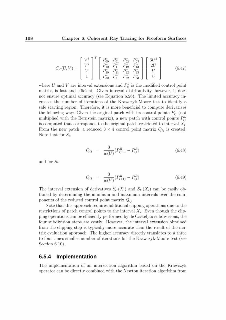
108 Chapter 6: Coherent Ray Tracing for Freeform Surfaces
SV (U, V ) =
V 3
V 2
V1
T
P ∗
00 P ∗
01 P ∗
02 P ∗
03
P ∗
10 P ∗
11 P ∗
12 P ∗
13
P ∗
20 P ∗
21 P ∗
22 P ∗
23
P ∗
30 P ∗
31 P ∗
32 P ∗
33
3U2
2UU0
(6.47)
where U and V are interval extensions and P ∗
ij is the modified control pointmatrix, is fast and efficient. Given interval distributivity, however, it doesnot ensure optimal accuracy (see Equation 6.26). The limited accuracy in-creases the number of iterations of the Krawczyk-Moore test to identify asafe starting region. Therefore, it is more beneficial to compute derivativesthe following way: Given the original patch with its control points Pij (notmultiplied with the Bernstein matrix), a new patch with control points PR
ij
is computed that corresponds to the original patch restricted to interval Xi.From the new patch, a reduced 3 × 4 control point matrix Qij is created.Note that for SU
Qij =3
w(U)(PR
ij+1 − PRij ) (6.48)
and for SV
Qij =3
w(V )(PR
i+1j − PRij ) (6.49)
The interval extension of derivatives SU(Xi) and SV (Xi) can be easily ob-tained by determining the minimum and maximum intervals over the com-ponents of the reduced control point matrix Qij.
Note that this approach requires additional clipping operations due to therestrictions of patch control points to the interval Xi. Even though the clip-ping operations can be efficiently performed by de Casteljau subdivisions, thefour subdivision steps are costly. However, the interval extension obtainedfrom the clipping step is typically more accurate than the result of the ma-trix evaluation approach. The higher accuracy directly translates to a threeto four times smaller number of iterations for the Krawczyk-Moore test (seeSection 6.10).
6.5.4 Implementation
The implementation of an intersection algorithm based on the Krawczykoperator can be directly combined with the Newton iteration algorithm from
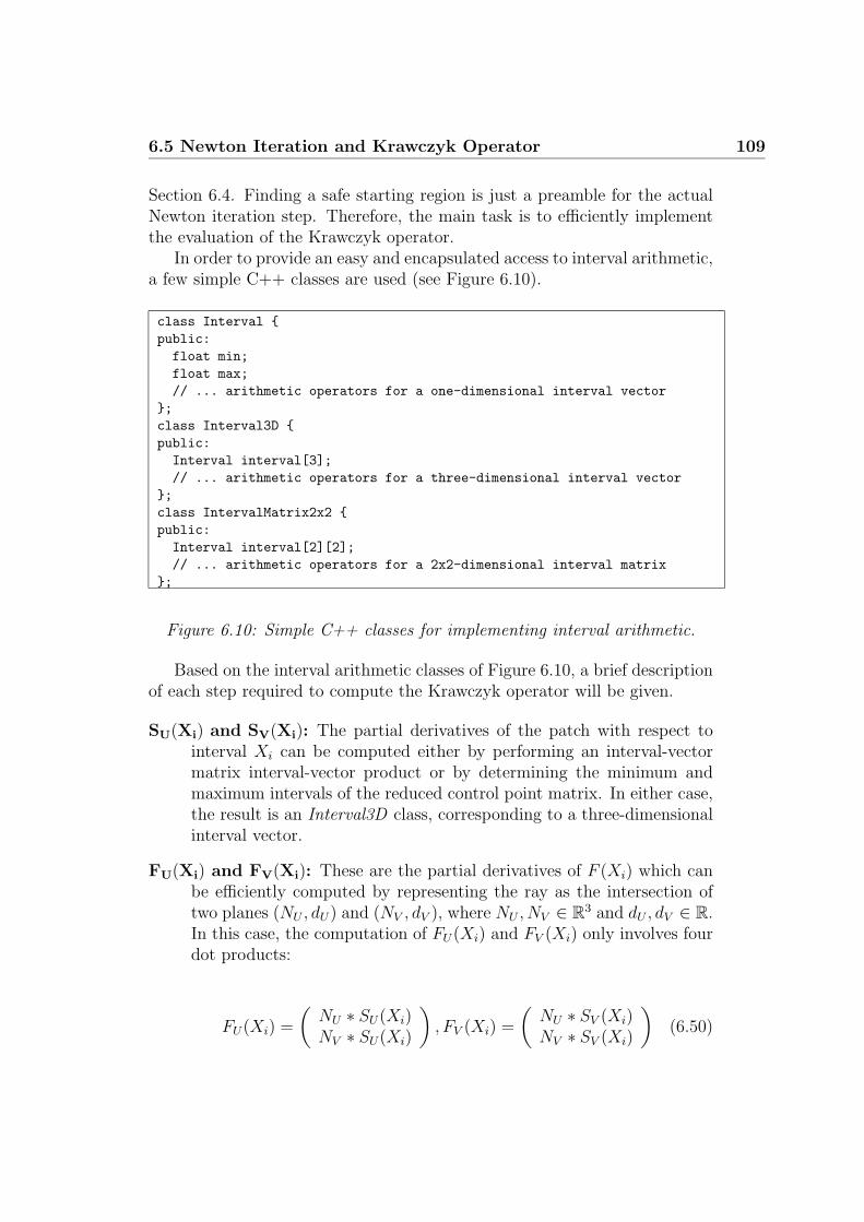
6.5 Newton Iteration and Krawczyk Operator 109
Section 6.4. Finding a safe starting region is just a preamble for the actualNewton iteration step. Therefore, the main task is to efficiently implementthe evaluation of the Krawczyk operator.
In order to provide an easy and encapsulated access to interval arithmetic,a few simple C++ classes are used (see Figure 6.10).
class Interval {
public:
float min;
float max;
// ... arithmetic operators for a one-dimensional interval vector
};
class Interval3D {
public:
Interval interval[3];
// ... arithmetic operators for a three-dimensional interval vector
};
class IntervalMatrix2x2 {
public:
Interval interval[2][2];
// ... arithmetic operators for a 2x2-dimensional interval matrix
};
Figure 6.10: Simple C++ classes for implementing interval arithmetic.
Based on the interval arithmetic classes of Figure 6.10, a brief descriptionof each step required to compute the Krawczyk operator will be given.
SU(Xi) and SV(Xi): The partial derivatives of the patch with respect tointerval Xi can be computed either by performing an interval-vectormatrix interval-vector product or by determining the minimum andmaximum intervals of the reduced control point matrix. In either case,the result is an Interval3D class, corresponding to a three-dimensionalinterval vector.
FU(Xi) and FV(Xi): These are the partial derivatives of F (Xi) which canbe efficiently computed by representing the ray as the intersection oftwo planes (NU , dU) and (NV , dV ), where NU , NV ∈ R
3 and dU , dV ∈ R.In this case, the computation of FU(Xi) and FV (Xi) only involves fourdot products:
FU(Xi) =
(
NU ∗ SU(Xi)NV ∗ SU(Xi)
)
, FV (Xi) =
(
NU ∗ SV (Xi)NV ∗ SV (Xi)
)
(6.50)

110 Chapter 6: Coherent Ray Tracing for Freeform Surfaces
The result of, e.g., NU ∗ SU(Xi) is a one-dimensional interval. There-fore, the result of FU(Xi) and FV (Xi) is stored into an IntervalMa-trix2x2 class, which is a 2 × 2 interval matrix.
Y = m(F′(Xi))−1: As FU(Xi) and FV (Xi) are partial derivatives of F (Xi),
the derivative of F (Xi) is the Jacobian matrix J = (FU(Xi)FV (Xi)).Before computing the inverse of the 2 × 2 Jacobian interval matrix J ,the midpoint operation m(Xi) is applied first. This transfers the 2× 2interval matrix into a real-valued 2×2 matrix. The inverse is computedby J−1 = adj(J)
detJ.
Aij = 12(w(F′(Xi)))ij: Performing the width operation transforms the previ-
ously computed 2×2 interval matrix into the real-valued 2 × 2 matrix A.
ei = 12(w(Xi))i: Computing ei only requires the width operator applied onthe current interval Xi.
f(y): The function f(y) = f(m(Xi)) can be quickly evaluated by performinga vector-matrix-vector product (see Section 6.4).
All these steps are required for an implementation of an intersection algo-rithm using the Krawczyk operator and Newton iteration. Figure 6.11 showsa pseudo C++ code for an example implementation.
In a first step, the algorithm performs a patch clipping operation (start-ing from the original patch) based on the current parametric interval UV.For implementing the Clip operation, the patch refinement code from Sec-tion 6.3 can be reused. Note that the clipping operation is performed in everyiteration of the algorithm and should therefore be as optimized as possible.
In order to avoid unnecessary iterations of the Krawczyk-Moore test, anearly pruning test is performed based on the axis-aligned bounding box of theclipped patch and the ray. If the ray intersects the bounding box, the partialderivatives (Su and Sv) of the clipped patch are computed and the resultsare stored in two three-dimensional interval vectors (su and sv). Figure 6.12shows an example implementation of Sv using SSE instructions.
The 2 × 2 interval matrix mat of the partial derivatives is computed byperforming four dot products between the patch derivatives su and sv andthe two ray plane equations (Nu,du) and (Nv,dv). This interval matrix formsthe basis for obtaining the two 2 × 2 real-valued matrices Y and A.
After evaluating the patch at the center of the current interval UV, thedistances fy of the corresponding point to the two ray planes are computed.The interval UV, the distances fy, and the matrices Y and A then allow forevaluating the Krawczyk operator (see Equation 6.34). If interval k returned

6.5 Newton Iteration and Krawczyk Operator 111
BicubicBezierPatch3D patch; Ray ray; // current patch and ray data
R3 Nu,Nv; float du,dv; // two ray planes (Nu,du) and (Nv,dv)
Interval2D stack[MAX_STACK_DEPTH];
Interval2D *sptr = stack;
*sptr++ = Interval2D(0.0f,0.0f,1.0f,1.0f);
while(sptr != stack) {
sptr--; Interval2D UV = *sptr; // get interval from stack
while(1) {
// -- clipped original patch based on current UV interval --
BicubicBezierPatchSSE clipped_patch = Clip(UV,patch);
// -- test if ray intersects bounding box of clipped patch --
Box box = clipped_patch.GetAABB();
if (!IntersectBox(ray,box)) break;
// -- compute interval extension of derivatives --
Interval3D su = Su(UV,clipped_patch);
Interval3D sv = Sv(UV,clipped_patch);
// -- compute interval matrix for partial derivatives --
IntervalMatrix2x2 mat = Fuv(su,sv,Nu,Nv);
// -- compute Matrix A and Y--
Matrix2x2 A,Y; A = ComputeA(mat); Y = ComputeY(mat);
// -- evaluate patch at the center of UV --
R3 p = Evaluate(patch,UV.center());
// -- compute distances to ray planes (Nu,du) and (Nv,dv) --
R2 fy = ComputeDistances(p,Nu,Nv,du,dv);
// -- compute new interval using the Krawczyk operator --
Interval2D k = ComputeKraw(UV,Y,A,fy);
if (Disjoint(UV,k)) break; // -- UV and k disjoint -> skip UV --
// -- compute subset of UV and k --
Interval2D UV_k = Subset(UV,k);
// -- if safe interval exists -> start Newton iteration --
if (isSafeInterval(UV,k,Y,A,fy)) {
NewtonIteration(UV_k,ray,patch); break;
} else {
// -- test if no reduction could be achieved --
if (UV_k == UV) {
// -- subdivide UV into four subsets, continue recursively --
Subdivide(UV,sptr[0],sptr[1],sptr[2],sptr[3]); sptr+=4; break;
}
UV = UV_k; // -- update UV interval --
} } }
Figure 6.11: Pseudo C++ Code for a ray-patch intersection algorithm usingthe Krawczyk-Moore test. The interval extension of the derivatives is com-puted by clipping the original patch according to the ’UV’ interval. If a safeinterval region is identified, a Newton iteration is performed.

112 Chapter 6: Coherent Ray Tracing for Freeform Surfaces
inline float hMax(const sse_t &a) {
const sse_t ftemp = _mm_max_ps(a,_mm_movehl_ps(a, a));
return _mm_cvtss_f32(_mm_max_ss(ftemp,_mm_shuffle_ps(ftemp,ftemp,1)));
}
inline float hMin(const sse_t &a) {
const sse_t ftemp = _mm_min_ps(a,_mm_movehl_ps(a, a));
return _mm_cvtss_f32(_mm_min_ss(ftemp,_mm_shuffle_ps(ftemp,ftemp,1)));
}
inline Interval3D Sv(const Interval2D &UV,
const BicubicBezierPatch3D &patch)
{
Interval3D S;
const Interval &V = UV.interval[1];
const float width = 3.0f / width(V);
// -- X --
const sse_t x0 = _mm_sub_ps(patch.p[1].t[0],patch.p[0].t[0]);
const sse_t x1 = _mm_sub_ps(patch.p[2].t[0],patch.p[1].t[0]);
const sse_t x2 = _mm_sub_ps(patch.p[3].t[0],patch.p[2].t[0]);
S.interval[0].min = width * hMin(_mm_min_ps(x0,_mm_min_ps(x1,x2)));
S.interval[0].max = width * hMax(_mm_max_ps(x0,_mm_max_ps(x1,x2)));
// -- Y --
const sse_t y0 = _mm_sub_ps(patch.p[1].t[1],patch.p[0].t[1]);
const sse_t y1 = _mm_sub_ps(patch.p[2].t[1],patch.p[1].t[1]);
const sse_t y2 = _mm_sub_ps(patch.p[3].t[1],patch.p[2].t[1]);
S.interval[1].min = width * hMin(_mm_min_ps(y0,_mm_min_ps(y1,y2)));
S.interval[1].max = width * hMax(_mm_max_ps(y0,_mm_max_ps(y1,y2)));
// -- Y --
const sse_t z0 = _mm_sub_ps(patch.p[1].t[2],patch.p[0].t[2]);
const sse_t z1 = _mm_sub_ps(patch.p[2].t[2],patch.p[1].t[2]);
const sse_t z2 = _mm_sub_ps(patch.p[3].t[2],patch.p[2].t[2]);
S.interval[2].min = width * hMin(_mm_min_ps(z0,_mm_min_ps(z1,z2)));
S.interval[2].max = width * hMax(_mm_max_ps(z0,_mm_max_ps(z1,z2)));
return S;
}
Figure 6.12: After clipping the original patch to the current interval ’UV, theinterval extension of patch derivatives (here in the parametric ’v’ direction)can be efficiently coded using SSE instructions. In a first step, a reducedcontrol point matrix (of the clipped patch) is created by subtracting controlpoint Pi+1j from Pij. For each of the three dimensions, the correspondinginterval is set to the minimum and maximum of the control point differences(multiplied by 3.0/width(V )).
by the Krawczyk operator and the current interval UV are disjoint, thecurrent interval UV is excluded from further processing.

6.6 Bezier Clipping 113
If one of the convergence criteria is fulfilled (isSafeInterval), the currentinterval UV is considered as a safe starting region and a Newton iteration-based intersection is performed. If no safe starting region can be determined,the algorithm performs a comparison of equality between the current intervalk and the subset of k and UV. If no reduction of the parametric region can beachieved, the algorithm subdivides UV into four sub-intervals and continuesrecursively. Otherwise, UV is replaced by the subset of k and UV, and thealgorithm continues. The algorithm terminates when the interval stack isempty.
6.5.5 Discussion
The main advantage of the Krawczyk operator is that it avoids the con-vergence problems of the standard Newton iteration-based intersection al-gorithm, providing reliable results. No additional spatial index structuresthat limit the parametric starting region are required. This reduces memoryrequirements because only the original patch data is needed.
However, identifying safe regions by evaluating the Krawczyk operatordoes not come for free. In each iteration, many complex operations, e.g. patchclipping or computing derivative intervals, have to be performed. Eventhough most operations can be efficiently implemented using SSE instruc-tions, significantly more SSE instructions are required than for standardNewton iteration-based intersection. For many scenes, this significantly im-pacts performance (see Section 6.10).
The number of iterations that are required to identify a safe convergenceregion largely depends on the size of the partial derivative intervals. Thelarger the derivative intervals, the smaller the reduction of the current para-metric region. Typically, the expansion of the derivative intervals becomeslarger with an increased patch curvature. Therefore, it might be beneficialto subdivide highly curved patches in a preprocessing step in order to firstreduce the curvature of these patches.
6.6 Bezier Clipping
Another approach for solving the intersection problem is the Bezier clippingalgorithm. Bezier clipping was first presented by Nishita et al. [Nishita90].The basic idea behind the Bezier clipping algorithm is to cut away regions ofthe patch (and therefore parametric intervals) that are known not to beintersected by the ray. Through continuous cutting, the parametric do-main associated with the remaining sub-patch converges to the solution.

114 Chapter 6: Coherent Ray Tracing for Freeform Surfaces
Note that Bezier clipping even works for rational Bezier surfaces or Beziercurves because all operations are only performed after a projection of thepatch into 2D.
The original algorithm proposed by Nishita et al. [Nishita90] suffers fromcertain numerical instabilities because of the underlying nature of the algo-rithm. Campagna et al. [Campagna97] identified those critical issues andproposed a modified version, which greatly reduced the numerical problems.
As a matter of fact, Bezier clipping is a very complex algorithm, whoseimplementation is not trivial. Nevertheless, even this complex algorithm canbe efficiently implemented using SSE instructions. In order to provide a bet-ter understanding of implementation issues, Section 6.6.1 will first discussthe original algorithm in detail. Section 6.6.2 will present a step-by-step ap-proach to an SSE implementation. Finally, Section 6.6.3 will deal remainingproblems and bottlenecks.
03
L
L u
v
00P P
33P30P −2
−1.5
−1
−0.5
0
0.5
1
1.5
2
0 0.2 0.4 0.6 0.8 1
umin
umax
u
BC(u)
Figure 6.13: Left Image: The distances of all 3D control points to the two rayplanes (blue lines) are determined, resulting in a 2D patch representation. Inorder to reduce the parametric domain, two lines Lu = 1
2(P30 − P00 + P33 −
P03) and Lv = 12(P03 − P00 + P33 − P30) are computed (green lines) which
pass through the origin and are roughly perpendicular to the two parametricdirections ’u’ and ’v’. Right Image: The convex hull of the distances of all 2Dcontrol points to line Lv, plotted using equidistant spacing of the unit interval.The region outside of the convex hull is known to not to be intersected andcan be cut away.
6.6.1 The Bezier Clipping Algorithm
Bezier clipping works by cutting away regions of the patch, and thus para-metric regions of the parameter domain, that are known not to be intersected

6.6 Bezier Clipping 115
by the ray. Each ray is again represented as the intersection of two planespl0(x) = N0 x + d0 and pl1(x) = N1 x + d1. In a first step, the distance forall control points Pij with respect to the two planes are computed
dij = (N0 Pij + d0, N1 Pij + d1) (6.51)
This allows for performing all cutting and subdivision operations in 2D in-stead of 3D, thus saving 33% of the total number of operations. The distancesdij are used as control points for the projected 2D patch representation
P′
(u, v) =3
∑
i=0
3∑
j=0
B3i (u)B3
j (v) dij , dij ∈ R2 (6.52)
The two lines pl0 and pl1 specify the coordinate axes, as shown in the leftimage of Figure 6.13. This reduces the intersection problem to finding valuesfor u and v, so that P
′
(u, v) = 0. The algorithm finds potential u and v valuesby iteratively excluding parametric regions with P
′
(u, v) 6= 0. Therefore, twolines Lu and Lv which pass through the origin are determined. Those linesshould be roughly perpendicular to the two parametric directions u and v,and are usually defined as:
Lu =1
2(P30 − P00 + P33 − P03) (6.53)
Lv =1
2(P03 − P00 + P33 − P30) (6.54)
In rare cases when either Lu = 0 or Lv = 0, the computation of Lu and Lv
must be performed differently [Efremov05]. If u is the first parametric direc-tion to be considered, the distances d
′
ij of all 2D control points to line Lu arecomputed next. Relying on the following property of Bernstein polynomials
n∑
i=0
i
nBn
i (u) = u (6.55)
an explicit Bezier curve can be defined as
BC(u) =n
∑
i=0
[
in
d′
i
]
Bni (u) (6.56)

116 Chapter 6: Coherent Ray Tracing for Freeform Surfaces
As BC(u) intersects the u-axis at some point where P′
(u, v) intersects Lu,the convex hull criteria for BC(u) can be applied in order to identify regionsfor u that do not intersect the u-axis and therefore do not intersect Lu ei-ther. The right image of Figure 6.13 shows the convex hull of the points( i
n, d
′
i) intersecting the u-axis at umin and umax. Therefore, intervals [0, umin]and [umax, 1] can be excluded from containing potential solutions in the udirection. Note that i
nis an equidistant spacing of the unit interval.
Two de Casteljau subdivision steps are now performed in the u directionin order to reduce the 2D Bezier patch P
′
(u, v) to the reduced parametricinterval [umin, umax]. The algorithm continues by alternating between u andv as parametric directions. Bezier clipping has three termination criteria:
• One interval is smaller than a predefined epsilon. If only one para-metric direction is still greater than epsilon, the algorithm continuesexclusively with the corresponding interval. If the interval for both di-rections is smaller than epsilon, the center of either interval is returnedas a valid intersection.
• After the de Casteljau subdivision, the subdivided patch does not in-clude the origin (with respect to the two ray planes), resulting in nointersection.
• The convex hull of the Bezier curve BC(u) does not intersect the u-axis,resulting in no intersection.
Handling multiple intersections can be problematic because the algorithmdoes not need to terminate in this case. A simple solution to this problem isto subdivide the patch in half and restart the algorithm with either halfprovided the parametric interval reduction is less than a constant value.Nishita [Nishita90] heuristically determined this value as being 20%.
If the algorithm converges to a solution, the original patch P (u, v) isevaluated at the corresponding parameter values in order to obtain the coor-dinates of the intersection point. By projecting the intersection point alongthe ray direction, distance t can be computed easily by
t = ray.direction ∗ (P (u, v) − ray.origin) (6.57)
6.6.2 SSE Implementation
The following operations required by the Bezier clipping algorithm have beenidentified as suitable core operations for implementation using SSE instruc-tions:

6.6 Bezier Clipping 117
struct BicubicBezierPatch2D
{
sse_t Nu_dist[4];
sse_t Nv_dist[4];
};
Figure 6.14: The structure stores the sixteen 2D control points of the patchP
′
(u, v), which are the distances dij of the original control points to the tworay planes, in an SSE suitable SOA format.
• Obtaining the 2D control points dij of patch P′
(u, v) by computing thedistances of the 3D control points Pij to the two ray planes pl0 and pl1.
• Checking whether the current patch P′
(u, v) includes the origin.
• Computing the Lu and Lv.
• Computing the distances d′
ij of dij to either Lu or Lv, and determiningthe convex hull of the obtained distance control points. Finding umin
and umax if the convex hull intersects the u-axis.
• Based on the reduced parametric interval [umin, umax], subdividing thecurrent patch two times in order to obtain sub-patch P
′
(u, v).
In the following, the implementation for all those operations will be dis-cussed in detail.
Initialization 3D to 2D
Applying the Bezier clipping algorithm for bicubic Bezier patches requiresa data structure for storing the 2D control points dij (see Figure 6.14) forthe 2D patch P
′
(u, v). This data structure is initialized by computing thedistances of the original control points to the two ray planes.
The code illustrated in Figure 6.15 shows that distances dij can be effi-ciently computed by performing a sequence of four dot products in parallel.Additionally, a pruning test is performed by checking the signs of the com-puted 2D distance coordinates. If all distances have matching signs, the 2Dconvex hull of all control points cannot contain the origin. Thus, the raycannot intersect the patch. Note that this additional test can be performedbasically without any additional costs.

118 Chapter 6: Coherent Ray Tracing for Freeform Surfaces
inline bool Init(const BicubicBezierPatch3D &patch,
const RayPlanesSSE &plane)
{
unsigned int signsU = 0;
for (unsigned int i=0;i<4;i++)
{
const sse_t d = _mm_add_ps(_mm_add_ps(_mm_mul_ps(plane.Nu.t[0],
patch.p[i].t[0]),
_mm_mul_ps(plane.Nu.t[1],
patch.p[i].t[1])),
_mm_mul_ps(plane.Nu.t[2],patch.p[i].t[2]));
const sse_t d_f = _mm_sub_ps(d,plane.du);
Nu_dist[i] = d_f;
signsU |= _mm_movemask_ps(d_f) << (4*i);
}
if (signsU == 0xffff || signsU == 0) return false;
unsigned int signsV = 0;
for (unsigned int i=0;i<4;i++)
{
const sse_t d = _mm_add_ps(_mm_add_ps(_mm_mul_ps(plane.Nv.t[0],
patch.p[i].t[0]),
_mm_mul_ps(plane.Nv.t[1],
patch.p[i].t[1])),
_mm_mul_ps(plane.Nv.t[2],patch.p[i].t[2]));
const sse_t d_f = _mm_sub_ps(d,plane.dv);
Nv_dist[i] = d_f;
signsV |= _mm_movemask_ps(d_f) << (4*i);
}
if (signsV == 0xffff || signsV == 0) return false;
return true;
}
Figure 6.15: Initialization of the sixteen 2D control points of patch P′
(u, v).The control points are the distances dij of the original control points to thetwo ray planes (stored in the SSE-suitable SOA format). If the new controlpoints lie completely in one half space with respect to a ray plane, the newpatch cannot contain the origin and the function returns false (early exit).
Origin Test
The test whether the current patch P′
(u, v) includes the origin, or not, isbasically the same as the previously mentioned sign test of all distances.Since this test is performed for every Bezier clipping iteration it needs to beas fast as possible. Therefore, a simplified version is chosen. This test firstcomputes the extremal distances (minimum and maximum) with respect to
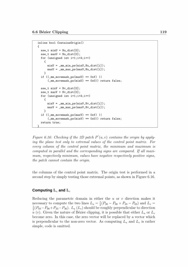
6.6 Bezier Clipping 119
inline bool ContainsOrigin()
{
sse_t minU = Nu_dist[0];
sse_t maxU = Nu_dist[0];
for (unsigned int i=1;i<4;i++)
{
minU = _mm_min_ps(minU,Nu_dist[i]);
maxU = _mm_max_ps(maxU,Nu_dist[i]);
}
if ((_mm_movemask_ps(maxU) == 0xf) ||
(_mm_movemask_ps(minU) == 0x0)) return false;
sse_t minV = Nv_dist[0];
sse_t maxV = Nv_dist[0];
for (unsigned int i=1;i<4;i++)
{
minV = _mm_min_ps(minV,Nv_dist[i]);
maxV = _mm_max_ps(maxV,Nv_dist[i]);
}
if ((_mm_movemask_ps(maxV) == 0xf) ||
(_mm_movemask_ps(minV) == 0x0)) return false;
return true;
}
Figure 6.16: Checking if the 2D patch P′
(u, v) contains the origin by apply-ing the plane test only to extremal values of the control point matrix. Forevery column of the control point matrix, the minimum and maximum iscomputed in parallel and the corresponding signs are compared. If all maxi-mum, respectively minimum, values have negative respectively positive signs,the patch cannot contain the origin.
the columns of the control point matrix. The origin test is performed in asecond step by simply testing those extremal points, as shown in Figure 6.16.
Computing Lu and Lv
Reducing the parametric domain in either the u or v direction makes itnecessary to compute the two lines Lu = 1
2(P30 − P00 + P33 − P03) and Lv =
12(P03−P00+P33−P30). Lu (Lv) should be roughly perpendicular to direction
u (v). Given the nature of Bezier clipping, it is possible that either Lu or Lv
become zero. In this case, the zero vector will be replaced by a vector whichis perpendicular to the non-zero vector. As computing Lu and Lv is rathersimple, code is omitted.
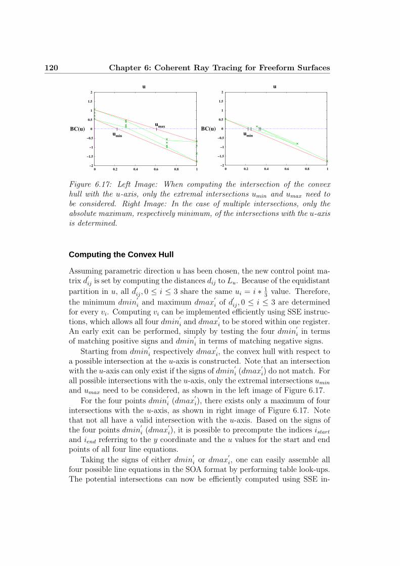
120 Chapter 6: Coherent Ray Tracing for Freeform Surfaces
−2
−1.5
−1
−0.5
0
0.5
1
1.5
2
0 0.2 0.4 0.6 0.8 1
umin
umax
u
BC(u)
−2
−1.5
−1
−0.5
0
0.5
1
1.5
2
0 0.2 0.4 0.6 0.8 1
umin
u
BC(u)
Figure 6.17: Left Image: When computing the intersection of the convexhull with the u-axis, only the extremal intersections umin and umax need tobe considered. Right Image: In the case of multiple intersections, only theabsolute maximum, respectively minimum, of the intersections with the u-axisis determined.
Computing the Convex Hull
Assuming parametric direction u has been chosen, the new control point ma-trix d
′
ij is set by computing the distances dij to Lu. Because of the equidistant
partition in u, all d′
ij, 0 ≤ i ≤ 3 share the same ui = i ∗ 13
value. Therefore,
the minimum dmin′
i and maximum dmax′
i of d′
ij, 0 ≤ i ≤ 3 are determinedfor every vi. Computing vi can be implemented efficiently using SSE instruc-tions, which allows all four dmin
′
i and dmax′
i to be stored within one register.An early exit can be performed, simply by testing the four dmin
′
i in termsof matching positive signs and dmin
′
i in terms of matching negative signs.
Starting from dmin′
i respectively dmax′
i, the convex hull with respect toa possible intersection at the u-axis is constructed. Note that an intersectionwith the u-axis can only exist if the signs of dmin
′
i (dmax′
i) do not match. Forall possible intersections with the u-axis, only the extremal intersections umin
and umax need to be considered, as shown in the left image of Figure 6.17.
For the four points dmin′
i (dmax′
i), there exists only a maximum of fourintersections with the u-axis, as shown in right image of Figure 6.17. Notethat not all have a valid intersection with the u-axis. Based on the signs ofthe four points dmin
′
i (dmax′
i), it is possible to precompute the indices istart
and iend referring to the y coordinate and the u values for the start and endpoints of all four line equations.
Taking the signs of either dmin′
i or dmax′
i, one can easily assemble allfour possible line equations in the SOA format by performing table look-ups.The potential intersections can now be efficiently computed using SSE in-

6.6 Bezier Clipping 121
struct IntersectionTableEntry // sixteen precomputed entries
{
unsigned int sy[4];
unsigned int ey[4];
float dx[4];
float sx[4];
};
// --------------------------------
sse_t dist[4];
const sse_t nx = _mm_set_ps1(du.y); // normal to Lu
const sse_t ny = _mm_set_ps1(-du.x);
for (unsigned int i=0;i<4;i++)
dist[i] = _mm_add_ps(_mm_mul_ps(nx,Nu_dist[i]),
_mm_mul_ps(ny,Nv_dist[i]));
sse_t min_dist = _mm_min_ps(_mm_min_ps(dist[0],dist[1]),
_mm_min_ps(dist[2],dist[3]));
sse_t max_dist = _mm_min_ps(_mm_max_ps(dist[0],dist[1]),
_mm_max_ps(dist[2],dist[3]));
if (_mm_movemask_ps(min_dist) == 0x0 ||
_mm_movemask_ps(max_dist) == 0xf) return false;
if ((minMask & 0x9) != 0x9) {
const unsigned int index = ((mask & 0x8) ? ~mask : mask) & 0x7;
const IntersectionTableEntry &entry = convexHullIntersectionTable[index];
const sse_t sy = _mm_setr_ps(ptr[(int)entry.sy[0]],ptr[(int)entry.sy[1]],
ptr[(int)entry.sy[2]],ptr[(int)entry.sy[3]]);
const sse_t ey = _mm_setr_ps(ptr[(int)entry.ey[0]],ptr[(int)entry.ey[1]],
ptr[(int)entry.ey[2]],ptr[(int)entry.ey[3]]);
const sse_t denom = Inverse(_mm_sub_ps(ey,sy));
const sse_t s = _mm_add_ps(_mm_mul_ps(_mm_mul_ps(*(sse_t*)entry.dx,sy),
denom),*(sse_t*)entry.sx);
const float s_min = _mm_cvtss_f32(sseHorizontalMin(s));
const float s_max = _mm_cvtss_f32(sseHorizontalMax(s));
minS = MIN(minS,s_min);
maxS = MAX(maxS,s_max);
}
if (((~maxMask) & 0x9) != 0x9) {
// ...
}
Figure 6.18: Given a maximum of four intersections, the indices for the fourline representations are precomputed, allowing the intersections to be effi-ciently computed in parallel. Horizontal operations then return the minimumand maximum of the ’u’ intersections.
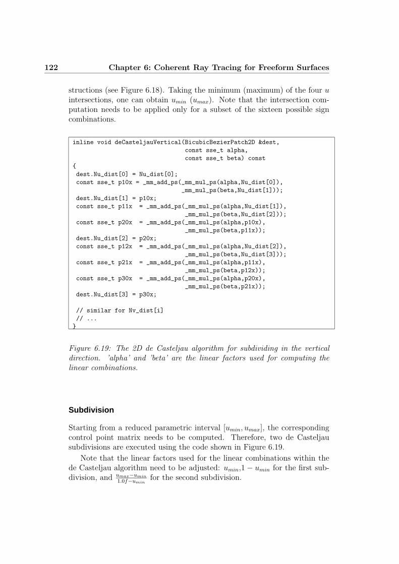
122 Chapter 6: Coherent Ray Tracing for Freeform Surfaces
structions (see Figure 6.18). Taking the minimum (maximum) of the four uintersections, one can obtain umin (umax). Note that the intersection com-putation needs to be applied only for a subset of the sixteen possible signcombinations.
inline void deCasteljauVertical(BicubicBezierPatch2D &dest,
const sse_t alpha,
const sse_t beta) const
{
dest.Nu_dist[0] = Nu_dist[0];
const sse_t p10x = _mm_add_ps(_mm_mul_ps(alpha,Nu_dist[0]),
_mm_mul_ps(beta,Nu_dist[1]));
dest.Nu_dist[1] = p10x;
const sse_t p11x = _mm_add_ps(_mm_mul_ps(alpha,Nu_dist[1]),
_mm_mul_ps(beta,Nu_dist[2]));
const sse_t p20x = _mm_add_ps(_mm_mul_ps(alpha,p10x),
_mm_mul_ps(beta,p11x));
dest.Nu_dist[2] = p20x;
const sse_t p12x = _mm_add_ps(_mm_mul_ps(alpha,Nu_dist[2]),
_mm_mul_ps(beta,Nu_dist[3]));
const sse_t p21x = _mm_add_ps(_mm_mul_ps(alpha,p11x),
_mm_mul_ps(beta,p12x));
const sse_t p30x = _mm_add_ps(_mm_mul_ps(alpha,p20x),
_mm_mul_ps(beta,p21x));
dest.Nu_dist[3] = p30x;
// similar for Nv_dist[i]
// ...
}
Figure 6.19: The 2D de Casteljau algorithm for subdividing in the verticaldirection. ’alpha’ and ’beta’ are the linear factors used for computing thelinear combinations.
Subdivision
Starting from a reduced parametric interval [umin, umax], the correspondingcontrol point matrix needs to be computed. Therefore, two de Casteljausubdivisions are executed using the code shown in Figure 6.19.
Note that the linear factors used for the linear combinations within thede Casteljau algorithm need to be adjusted: umin,1 − umin for the first sub-division, and umax−umin
1.0f−umin
for the second subdivision.

6.7 Summary of Intersection Algorithms 123
Step CPU Cycles
Initialization 3D to 2D 74Origin Test 70Computing Lu and Lv 50Computing Convex Hull 218Subdivision 100 (200)
Table 6.4: Average number of CPU cycles for each of the core operationsfor Bezier clipping. The two most expensive operations are the determina-tion of the convex hull including intersection computation, and the relatedsubdivision. Note that subdivision in ’u’ direction requires additional shuffleinstructions, thereby roughly doubling the costs.
6.6.3 Discussion
Table 6.4 shows the average number of cycles for different core operations.Almost all core operations require less than 100 cycles. The cost, in particu-lar, for computing the convex hull and for patch subdivision, could be furtherreduced as soon as processor architectures offer better support for horizontaland shuffle operations.
The Bezier clipping algorithm in its original form does not depend on anadditional per-patch spatial index structure as required by the Newton itera-tion. Similar to the uniform refinement approach, it only requires the originalcontrol point matrix, which makes it very memory efficient. Nevertheless, theBezier clipping algorithm could also benefit from a patch acceleration struc-ture to speed up convergence. Restricting the parametric starting domainassociated to an index structure entry would immediately reduce the numberof required iterations.
Another difficulty is that the Bezier clipping algorithm is rather sensitiveto the relation of the two lines Lu and Lv. Ideally, these two vectors should beperpendicular to each other. In practice, however, the angle between themcan be rather small. In this case, only a low reduction of the parametricdomain can be achieved, resulting in an increased number of iterations. Itwould be interesting to implement the approach proposed by Efremov etal. [Efremov05] for computing more suitable Lu and Lv vectors.
6.7 Summary of Intersection Algorithms
Except for the standard Newton iteration-based intersection, none of the de-scribed approaches depend on an additional per-patch spatial index structure.

124 Chapter 6: Coherent Ray Tracing for Freeform Surfaces
However, Bezier clipping or Newton iteration using the Krawczyk operatormight benefit from a structure of this kind. Such an index structure wouldrestrict the parametric starting region, thereby improving convergence of theintersection algorithm. Moreover, if an intersection algorithm requires manyiterations before pruning a patch, a per-patch index structure can help toperform the pruning test earlier (in the traversal phase). On the other hand,the increased number of traversal steps and memory accesses can offset thebenefit gained from a higher convergence speed.
Profiling tools such as VTune [Intel04] show that for all approaches whichdo not rely on additional spatial index structures, the intersection sequenceis compute-bound. A stack of subdivided patches (or parametric intervals),as required by most approaches, comprises only a few KB. Therefore, stackdata completely resides in the cache hierarchy.
The only point where cache misses appear is the point of accessing patchdata. However, most of those (L2) cache misses can be avoided by prefetchingdata for the subsequent patches while intersecting the current one. Sincethe memory latency is usually smaller than the costs of patch intersection,memory prefetching works very well in this situation.
Comparing the implementation complexity of the different intersectionalgorithms shows that the intersection based on uniform refinement employthe shortest core routines and the simplest control flow. A slightly morecomplex algorithm is the Newton iteration with an additional spatial indexstructures over sub-patches, while Bezier clipping is the most complex in-tersection algorithm. Newton iteration using the Krawczyk operator is ascomplex as Bezier clipping. Whenever short construction times are manda-tory, e.g. for supporting dynamic scenes (see Chapter 7), one should choosean intersection algorithm that does not depend on additional per-patch spa-tial index structures. Furthermore, if limited accuracy is acceptable, uniformrefinement typically provides the highest performance (see Section 6.10). Foractual performance statistics for ray tracing complete bicubic Bezier scenes,see Section 6.10.
When it comes to supporting ray bundles, uniform refinement and Newtoniteration with a sub-patch spatial index structure provide a straightforwardextension. Integrating ray bundles into Bezier clipping is more difficult be-cause the subdivision has to be done on a per ray basis. Moreover, Bezierclipping requires numerous temporary data updates, which is difficult to re-alize for many rays in parallel. Therefore, it is likely that the benefit ofcomputing the intersection for multiple rays in parallel will be offset by theadditional overhead.
For a Newton iteration-based intersection algorithm using the Krawczykoperator the support of ray bundles is non-trivial. As each ray uses its own

6.8 Spatial Index Structures for Patches 125
parametric interval, the patch clipping step must be performed individuallyfor each ray.
On the other hand, it might be beneficial to split the intersection algo-rithm into a serial and a parallel part: This means evaluating the Krawczykoperator for each ray in a serial process, but performing the computation forthe subsequent Newton iterations in parallel.
6.8 Spatial Index Structures for Patches
Having a fast primitive intersection code is only a first step, because typicalscenes are comprised of many primitives which will require the constructionof a spatial index structure to reduce the number of ray-patch intersectiontests per ray. Compared to a simple ray-triangle intersection, the cost fora ray-patch intersection is significantly higher. This means that a smallnumber of ray-patch intersection tests per ray is essential for achieving highperformance, which puts certain quality requirements on the spatial indexstructure used. In the past, researchers mostly used bounding volume hi-erarchies [Rubin80, Kay86, Haines91, Smits98] as the spatial accelerationstructure for reducing the number of ray-patch intersection tests. Because ofthe very fast traversal code (see Chapter 4) and its adaptation ability withrespect to geometric distribution, a kd-tree is chosen as the spatial indexstructure.
A kd-tree over patches is built based on the axis-aligned bounding boxes(AABB) for each patch, ignoring the patch shape itself. Even though thissimplification is less accurate, it is both simple and fast. To enhance thequality of the kd-tree, a surface area heuristic (SAH) [Havran01, Wald04,Benthin04] is applied to carefully position the splitting plane. This resultsin better quality (fewer intersection tests per ray), compared to a standardkd-tree construction algorithm. For a more detailed discussion of how toconstruct kd-trees out of axis-aligned bounding boxes, see Section 7.1.
6.9 Trimming Curves
Trimming curves are a common method for overcoming the topologicallyrectangular limitations of patches. Trimming curves, which are defined intwo-dimensional parameter space, are mostly used when designers wish tocut out sections from patches.
Similar to the conversion of NURBS to bicubic Bezier patches (see Sec-tion 6.2), an arbitrary source representation for a trimming curve is converted
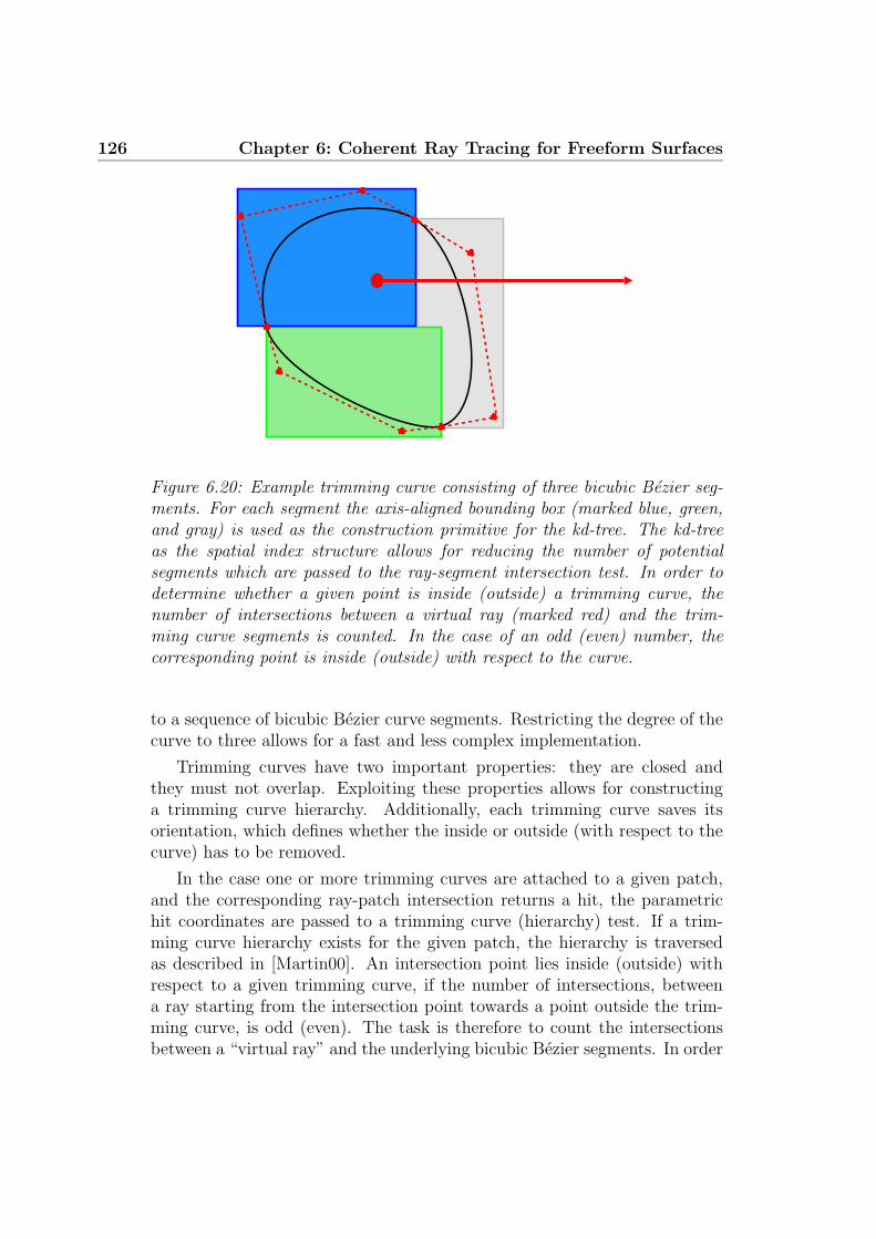
126 Chapter 6: Coherent Ray Tracing for Freeform Surfaces
Figure 6.20: Example trimming curve consisting of three bicubic Bezier seg-ments. For each segment the axis-aligned bounding box (marked blue, green,and gray) is used as the construction primitive for the kd-tree. The kd-treeas the spatial index structure allows for reducing the number of potentialsegments which are passed to the ray-segment intersection test. In order todetermine whether a given point is inside (outside) a trimming curve, thenumber of intersections between a virtual ray (marked red) and the trim-ming curve segments is counted. In the case of an odd (even) number, thecorresponding point is inside (outside) with respect to the curve.
to a sequence of bicubic Bezier curve segments. Restricting the degree of thecurve to three allows for a fast and less complex implementation.
Trimming curves have two important properties: they are closed andthey must not overlap. Exploiting these properties allows for constructinga trimming curve hierarchy. Additionally, each trimming curve saves itsorientation, which defines whether the inside or outside (with respect to thecurve) has to be removed.
In the case one or more trimming curves are attached to a given patch,and the corresponding ray-patch intersection returns a hit, the parametrichit coordinates are passed to a trimming curve (hierarchy) test. If a trim-ming curve hierarchy exists for the given patch, the hierarchy is traversedas described in [Martin00]. An intersection point lies inside (outside) withrespect to a given trimming curve, if the number of intersections, betweena ray starting from the intersection point towards a point outside the trim-ming curve, is odd (even). The task is therefore to count the intersectionsbetween a “virtual ray” and the underlying bicubic Bezier segments. In order
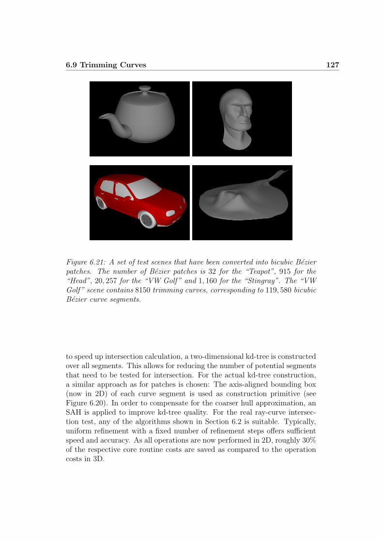
6.9 Trimming Curves 127
Figure 6.21: A set of test scenes that have been converted into bicubic Bezierpatches. The number of Bezier patches is 32 for the “Teapot”, 915 for the“Head”, 20, 257 for the “VW Golf” and 1, 160 for the “Stingray”. The “VWGolf” scene contains 8150 trimming curves, corresponding to 119, 580 bicubicBezier curve segments.
to speed up intersection calculation, a two-dimensional kd-tree is constructedover all segments. This allows for reducing the number of potential segmentsthat need to be tested for intersection. For the actual kd-tree construction,a similar approach as for patches is chosen: The axis-aligned bounding box(now in 2D) of each curve segment is used as construction primitive (seeFigure 6.20). In order to compensate for the coarser hull approximation, anSAH is applied to improve kd-tree quality. For the real ray-curve intersec-tion test, any of the algorithms shown in Section 6.2 is suitable. Typically,uniform refinement with a fixed number of refinement steps offers sufficientspeed and accuracy. As all operations are now performed in 2D, roughly 30%of the respective core routine costs are saved as compared to the operationcosts in 3D.

128 Chapter 6: Coherent Ray Tracing for Freeform Surfaces
6.10 Results
This section will provide performance statistics and analyses for ray tracingbicubic Bezier scenes. For testing purposes, four scenes with different com-plexity have been used (see Figure 6.21). Note that only the “VW Golf”scene contains trimming curves.
Comparing the different intersection approaches is difficult. This is espe-cially true when it comes to comparing uniform refinement with approachesbased on analytical solutions. Therefore, the algorithmic analysis is split intotwo parts: The first part covers intersection for uniform refinement while thesecond part deals with the analytical algorithms.
Regardless of the intersection algorithm, ray tracing of Bezier patches re-quires less time in kd-tree traversal than for triangles. Even if an additionalindex structures over sub-patches is used, typically only 20-30% of the timefor tracing a single ray is spent in kd-tree traversal, while ray-patch intersec-tion takes up 70-80% of the time. The performance impact of fast traversalcode is therefore less than for ray tracing triangles (typically traversal 70%,intersection 30%). The simple reason for this is that total performance isexclusively determined by the intersection step. Even though the cost forintersection already starts to dominate even in the triangle case, for Bezierpatches the cost discrepancy between traversal and intersection is even moresignificant. In the case no sub-patch index structures are used, a kd-tree overpatches is shallower as compared to the triangle case. This results in 40-50%fewer traversal steps in total, additionally shifting the dominating cost factortowards intersection.
Rays Teapot VW Golf Head Stingray
1 378760 704965 219687 44089216 6.71% 10.21% 10.6% 8.74%
Table 6.5: Average number of patches loaded per frame at a resolution of640×480, casting only primary rays. Compared to tracing single rays, tracingray bundles of sixteen rays reduces patch accesses to less than 10% of thenumber for individual rays.
Extending single ray traversal to ray bundle traversal allows for exploitingthe same benefits as those of the triangle case. In particular, any fast traversalcode can be reused directly. Only the code for triangle intersections has to bereplaced by patch intersection code. Moreover, a similar bandwidth reductionas for triangles can be achieved, because neighboring rays are likely to accessthe same patches. The loaded patch data can therefore be reused for all rays

6.10 Results 129
within the bundle. This reduces the total number of patch accesses per frame,and therefore the required bandwidth to memory. Table 6.5 shows that for4 × 4 ray bundles, the bandwidth required for loading patch data can bereduced to less than 10% of the original amount. For scenes with additionalsub-patch index structures, the reduction is typically smaller (depending onthe depth of the sub-patch index structure).
0
1
2
3
4
5
6
0 2 4 6 8 10 12
fram
es p
er s
econ
d
refinement steps
TeapotVW Golf
HeadStingray
Figure 6.22: (Single ray) performance (in fps) for Bezier scenes as a functionof the number of patch refinement steps. Each refinement step corresponds toa de Casteljau subdivision step in one of the two parametric directions. Allexperiments were performed at a resolution of 640 × 480 pixels on a singlePentium-IV 2.2 GHz processor. Using 4−6 refinement steps, an intersectionbased on uniform refinement is able to achieve interactive performance on asingle processor.
6.10.1 Uniform Refinement Results
In order to demonstrate the impact of an increasing refinement level, Fig-ure 6.22 illustrates the performance in frames per second for all four testscenes, casting a single primary ray per pixel. All tests were run on a singlePentium-IV 2.2 GHz processor at a resolution of 640× 480. Even for a highnumber of refinement steps, interactive performance is realized. The achievedaccuracy depends to a great extent on the patch shape itself, but for most

130 Chapter 6: Coherent Ray Tracing for Freeform Surfaces
Rays Teapot VW Golf Head Stingray
1 2.0 1.01 3.23 1.8916 16.14 5.72 12.93 9.02Speedup 8.07x 5.67x 4.0x 4.77x
Table 6.6: Performance comparison between tracing single rays and tracingbundles of sixteen rays, in frames per second. All scenes are rendered at aresolution of 640×480, casting only primary rays and with a refinement levelof 4. Tracing ray bundles of sixteen rays results in a speedup factor of 4− 8,compared to tracing single rays. For the “VW Golf” scene, no evaluation oftrimming curves has been applied.
applications a refinement level of 4 − 6 already provides smooth surfaces.
To further improve performance, the single ray intersection code was ex-tended in order to support ray bundles. Uniform refinement, in particular,can benefit enormously from ray bundles because the patch subdivision costcan be efficiently amortized over all rays within the bundle. As for the tri-angle case, a bundle size of 16 rays has been found to be most beneficial.
A comparison between the fastest code for tracing single rays and thefastest code for tracing ray bundles shows that a speedup factor of 4 − 8 isachieved through bundling (see Table 6.6). By increasing coherence withinthe ray bundle, e.g. by rendering at resolutions higher than 640 × 480, thisfactor can be increased even further.
Rays Teapot VW Golf Head Stingray
640 × 480 8.07 5.67 4.0 4.77800 × 600 8.25 6.61 4.48 5.171024 × 1024 8.6 8.42 5.64 6.281600 × 1200 8.7 8.5 5.7 6.41Speedup 7.8% 49.91% 42.5% 34.38%
Table 6.7: Speedup improvement for tracing ray bundles compared to tracingsingle rays with increasing resolution. The more coherent the rays are, thehigher the speedup improvement (up to 49.91%).
Table 6.7 shows the increase of the speedup factor for all test scenes whenrendered at different resolutions. At a resolution of 1024×1024, the increasedcoherence within the ray bundle results in a 49.91% speedup as compared torendering at a resolution of 640 × 480.
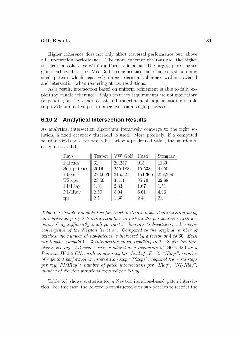
6.10 Results 131
Higher coherence does not only affect traversal performance but, aboveall, intersection performance. The more coherent the rays are, the higherthe decision coherence within uniform refinement. The largest performancegain is achieved for the “VW Golf” scene because the scene consists of manysmall patches which negatively impact decision coherence within traversaland intersection when rendering at low resolutions.
As a result, intersection based on uniform refinement is able to fully ex-ploit ray bundle coherence. If high accuracy requirements are not mandatory(depending on the scene), a fast uniform refinement implementation is ableto provide interactive performance even on a single processor.
6.10.2 Analytical Intersection Results
As analytical intersection algorithms iteratively converge to the right so-lution, a fixed accuracy threshold is used. More precisely, if a computedsolution yields an error which lies below a predefined value, the solution isaccepted as valid.
Rays Teapot VW Golf Head Stingray
Patches 32 20,257 915 1160Sub-patches 2016 255,188 15,538 4,650IRays 273,663 215,821 151,365 252,399TSteps 23.59 35.11 35.70 22.88PI/IRay 1.01 2.33 1.67 1.51NI/IRay 2.59 8.04 5.61 4.93fps 2.5 1.35 2.4 2.0
Table 6.8: Single ray statistics for Newton iteration-based intersection usingan additional per-patch index structure to restrict the parametric search do-main. Only sufficiently small parametric domains (sub-patches) will ensureconvergence of the Newton iteration. Compared to the original number ofpatches, the number of sub-patches is increased by a factor of 4 to 60. Eachray invokes roughly 1 − 3 intersection steps, resulting in 2 − 8 Newton iter-ations per ray. All scenes were rendered at a resolution of 640 × 480 on aPentium-IV 2.2 GHz, with an accuracy threshold of 1E−3. “IRays”: numberof rays that performed an intersection step,”TSteps”: required traversal stepsper ray,“PI/IRay”: number of patch intersections per “IRay”, “NI/IRay”:number of Newton iterations required per “IRay”.
Table 6.8 shows statistics for a Newton iteration-based patch intersec-tion. For this case, the kd-tree is constructed over sub-patches to restrict the

132 Chapter 6: Coherent Ray Tracing for Freeform Surfaces
parametric search domain. The Newton iteration will only converge if theparametric starting region is sufficiently small. As convergence depends to agreat extent on patch curvature, a simple criterion based on the deviation toa bilinear patch is used to terminate the generation of sub-patches. Depend-ing on the scene, 4 to 60 times more sub-patches than patches have to becreated in order to ensure convergence. Note that for sub-patches, no actualpatch data needs to be stored, but only a reference to the correspondingparametric domain as well as a reference to the original patch data. All re-quired information can be efficiently stored in a 32-byte structure [Geimer05],requiring 7.78 MB of additional storage space for 215, 821 sub-patches of the“VW Golf” scene. As the kd-tree is constructed over sub-patches, the corre-sponding storage space increases from 3.14 MB for 20, 257 patches to 62.36MB for 255, 188 sub-patches.
As illustrated in Table 6.8, one ray requires an average of 22−35 traversalsteps and 1−3 intersection tests. Each intersection step requires at least oneNewton iteration, resulting in 2 − 8 Newton iterations per ray on average.Given the small number of required iterations and the impact of the efficientSSE implementation (see Section 6.4), interactive performance even on asingle processor is achieved.
Rays Teapot VW Golf Head Stingray
Patches 32 20257 915 1160IRays 273,663 215,821 151,365 252,399TSteps 10.22 24.64 23.12 16.63PI/IRay 1.31 3.26 2.08 1.71BC/IRay 9.96 2.03 2.31 2.48fps 0.8 1.25 2.37 1.73
Table 6.9: Single ray statistics for Bezier clipping-based intersection. Eachray invokes 1− 3 intersection steps, resulting in 2− 10 Bezier clipping stepsper ray. All scenes were rendered at a resolution of 640 × 480 on a 2.2GHz Pentium-IV, with a solution accuracy of 1E − 3. “IRays”: numberof rays that performed an intersection step, “PI/IRay”: number of patchintersections per “IRay”, “BC/IRay”: number of Bezier clipping iterationsrequired per “IRay”.
Intersection based on Bezier clipping, as illustrated in Table 6.9, does notdepend on additional data structures in order to ensure convergence. As aresult, the kd-tree is significant smaller, resulting in up to 50% fewer traver-sal steps compared to the sub-patch-based intersection. For most scenes,

6.10 Results 133
only 2− 3 Bezier clipping iterations are required. As with Newton iteration-based intersection, the “Teapot” with its highly curved patches requires sig-nificantly more iterations (more pre-subdivisions) than all other scenes. Aperformance comparison between the two intersection approaches shows thatthe costs for Bezier clipping cannot be compensated for by the smaller num-ber of traversal steps. Bezier clipping provides a slightly lower performancethan Newton iteration-based intersection but, on the other hand, requires noadditional spatial index structures.
Rays Teapot VW Golf Head Stingray
Patches 32 20257 915 1160IRays 273,663 215,821 151,365 252,399TSteps 10.22 24.64 23.12 16.63PI/IRay 1.31 3.26 2.08 1.71KI-Clip/IRay 12.76 6.01 4.53 4.65KI-Interval/IRay 44.23 22.82 14.49 14.89NI/IRay 0.53 1.76 0.87 0.83fps 0.21 0.25 0.52 0.43
Table 6.10: Single ray statistics for Newton iteration-based intersection usingthe Krawczyk operator. All scenes were rendered at a resolution of 640× 480on a 2.2 GHz Pentium-IV, with a solution accuracy of 1E − 3. “IRays”:number of rays that performed an intersection step, “PI/IRay”: number ofpatch intersections per “IRay”, “KI-Clip/IRay”: number of Krawczyk opera-tor evaluations per “IRay”, using a clipping operation to compute the inter-val extension of the partial patch derivatives,“KI-Interval/IRay”: number ofKrawczyk operator evaluations per “IRay”, using pure interval arithmetic tocompute the interval extension of the partial patch derivatives, “NI/IRay”:number of Newton iterations required per “IRay”.
Table 6.10 shows statistics for Newton iteration-based intersection usingthe Krawczyk operator. The algorithm does not rely on additional per-patchspatial index structures, which implies the same number of traversal andintersection steps per ray as for Bezier clipping. In terms of iterations forthe Krawczyk-Moore test, the higher accuracy of the interval extension of thepartial derivatives makes for a reduction of up to a factor of four as comparedto using pure interval arithmetic.
As the “Teapot” scene contains highly curved patches, the Krawczykoperator using clipping operations still needs over 12 iterations per ray, ascompared to 4 − 6 for the other scenes, to provide safe starting intervals.
134 Chapter 6: Coherent Ray Tracing for Freeform Surfaces
Moreover, the safe starting intervals are typically very small which allowsfor fast convergence of the Newton iteration. For the four test scenes, only0.5− 2 iterations per ray are required in order to compute the final intersec-tion. However, total performance is lower than with the standard Newtoniteration-based algorithm. The reasons behind the lower performance are thecostly operations required for evaluating the Krawczyk operator. Further op-timization should thus concentrate on reducing the cost for these operations.
As only the “VW Golf” scene includes trimming curves, the impact oftrimming curve evaluation could only be measured for this scene. Dependingon the view, additional trimming curve tests cause a total performance de-crease of 10−30% (compared to the performance statistics of Tables 6.8, 6.9,and 6.10).
Extending ray-patch intersection algorithms to efficiently support raybundles is difficult. Certain algorithms, e.g. Bezier clipping or Newton it-eration using the Krawczyk operator, cannot be easily extended to efficientlysupport ray bundles because these algorithms require many complex opera-tions as well as a complex control flow. Implementing these operations forray bundles is likely to introduce additional implementation overhead. Thisis not the case for the standard Newton iteration-based intersection. Ta-ble 6.11 illustrates statistics for 2 × 2 ray bundles using standard Newtoniteration-based intersection. At a resolution of 1024 × 1024, ray bundles al-low for achieving a speedup factor of 1.58 to 2.13, compared to tracing singlerays. An interesting point is that the number of iterations for ray bundles isonly slightly increased, even though the exit point is not taken unless all fourrays fulfill the exit criteria. This indicates high decision coherence within thealgorithm.
The speedup for ray bundles could be even higher, but the small numberof registers and the limited floating point capability of current CPU architec-tures have a negative impact on intersection performance. These limitationssignificantly affect bundles larger than 2 × 2 rays. For such larger bundles,standard Newton iteration-based intersection is sub-optimal. For every ac-cessed sub-patch, a complete intersection test for all rays within the bundles,has to be performed (as long as not all bundles have a valid intersection).Many small sub-patches (caused by patch curvature), increase the probabil-ity that a high number of sub-patches, will need to be accessed, until all rayswithin the bundle have found a valid intersection.
Assuming future CPU architectures will have a higher number of registersand a improved support for floating point computations, a Newton iteration-based intersection algorithm using the Krawczyk operator might then bebeneficial. The Krawczyk operator would return, for each ray within thebundle, either a valid starting interval or the statement that the ray will

6.11 Application 135
Rays Teapot VW Golf Head Stingray
TSteps 26.71 35.33 35.67 20.83PI/IRay 1.25 2.47 1.71 1.66NI/IRay 3.28 8.31 5.29 5.19fps 0.68 0.41 0.56 0.54TSteps 2 × 2 26.62 35.41 32.69 20.9PI/IRay 2 × 2 1.35 3.11 2.04 1.91NI/IRay 2 × 2 3.76 11.5 5.29 6.40fps 1.45 0.65 0.93 0.98Speedup 2.13x 1.58x 1.66x 1.81x
Table 6.11: Comparison of Newton iteration-based intersection for single raysagainst bundles of 2 × 2 rays. All scenes were rendered at a resolution of1024 × 1024, with a solution accuracy of 1E − 3. Even though the exit pointwithin the Newton iteration is not taken unless the criteria are fulfilled by allfour rays, the required number of Newton iterations is only slightly increased.Therefore, a performance speedup factor of 1.58 to 2.13 is achieved, comparedto casting single rays.
miss the patch. Because of the complex control flow, it might prove useful toperform these operations sequentially. The result of this operation sequencewould be an array of starting intervals as well as a bit-mask to indicatewhether a ray will intersect a given patch or not. Based on these values aparallel Newton iteration could be performed for all rays within the bundle.The iteration would stop once all valid rays (for which a safe starting regionhas been identified) indicate a valid intersection.
Obviously, all traversal algorithms from Section 4.2, e.g. reducing traver-sal steps by finding better kd-tree entry points, could be applied here. How-ever, most of the total time is spent in intersection, which limits the positiveimpact of a smaller number of traversal steps. The main goal should thereforebe to further optimize intersection.
6.11 Application
Computer-Aided Design and Virtual Reality are becoming increasingly im-portant tools for industrial design applications. Large and high-end engi-neering projects, in particular, such as cars or airplanes, are already beingdesigned on an almost entirely digital basis, as the cost for building physicalmockups of such objects is very high.

136 Chapter 6: Coherent Ray Tracing for Freeform Surfaces
Figure 6.23: Top left: Mercedes C-class model directly exported from a CADsystem and converted into 319, 340 bicubic Bezier patches and 1.46 million(bicubic Bezier) trimming curves. The patches are ray traced directly withouttriangulation. Top right: In order to illustrate the complexity of the Mercedesmodel, a random color is assigned to each patch. Center left: The modelwith advanced shading for glass and car paint, combined with surroundinggeometry and an HDR environment map. Center right, Bottom left, Bottomright: Close-ups demonstrating the high geometric accuracy necessary forhigh-quality visualization of smooth surfaces.
6.11 Application 137
CAD engineers work on the raw geometric data of the model, usuallyusing freeform data such as NURBS surfaces [Piegl97]. In order to satisfythe requirement of interactivity, practically all of today’s virtual reality (VR)systems are built on triangle rasterization hardware. With this, however,rendering complete models with high geometric accuracy is not possible, asfreeform surfaces usually cannot be rendered directly, and the number oftriangles generated by a high-quality tessellation is in the order of tens ofmillions of triangles.
The process of tessellating freeform models, which consists of convertingthem first to triangles and subsequently carrying out a simplification step,is currently state-of-the-art in the industry. However, this approach hastwo important drawbacks: First, only limited geometric accuracy is achievedand, second, preparing these special VR models takes time, so changes ofthe original model may take up to several days before they can be shown ina VR presentation. This often leads to decision makers looking at outdatedmodel variants.
Thanks to the seamless integration of fast intersection implementationsfor freeform surfaces (see Chapter 6) into the ray tracing framework, it isnow possible to deliver the level of interactive performance which is requiredfor VR systems. Moreover, ray tracing-based rendering algorithms allow forachieving higher shading quality than rasterization-based VR systems couldprovide.
Figure 6.23 shows examples of a ray tracing-based VR system which uti-lized the fast freeform ray tracing code from Chapter 6. The model consistedof 69, 067 NURBS surfaces and 392, 491 2D NURBS curves forming 73, 749trimming curves, directly exported from a CAD system. The 69, 067 NURBSsurfaces were converted into 308, 095 Bezier patches of arbitrary degree. Inorder to fully exploit the fast patch intersection code of the previous sec-tion, a patch degree reduction was applied, yielding 319, 340 bicubic Bezierpatches. Degree reduction was applied in a similar way for the 2D NURBScurves, resulting in 1.46 million bicubic Bezier curves, i.e. 5 trimming curvesper patch. Besides the geometry itself, extremely complex shading, e.g. so-phisticated car paint or glass shading, was applied to provide as much realismas possible.
A cluster of 15 dual-processor PCs (a mix of 3.0 GHz Intel Pentium-IVs and 2.4 GHz Opterons) was used to provide enough compute powerfor performing all ray tracing and shading tasks at interactive rates (seeChapter 8). This setup allowed for achieving high-quality rendering with aframe rate of up to 10 frames per second, at a resolution of 640 × 480. Asthe underlying shading system only supports single rays, neither ray bundletraversal nor ray bundle intersection were used.

138 Chapter 6: Coherent Ray Tracing for Freeform Surfaces
Apart from the direct support of CAD data, the ray tracing-based VRprototype system shows the advantage of a decoupled ray tracing and shadingprocess. The complete shading framework, in particular, is fully independentof the underlying geometry and was developed using triangular models. Inorder to render bicubic Bezier patches, only the underlying core ray tracingalgorithm had to be extended to support patches.
6.12 Conclusions and Future Work
This chapter has shown that by optimizing algorithms and adapting themto the underlying processor architecture, interactive ray tracing of freeformsurfaces can be realized even on a single processor. However, for a highlyaccurate analytical solution, the computing power of a single processor isnot enough in order to provide high frame rates. If future processor archi-tectures provide improved support for SSE execution, e.g. more registers andexecution pipelines, all proposed intersection algorithms will benefit directly.
Even though Newton iteration-based intersection using the Krawczyk op-erator is the slowest algorithm, it has the important advantage of providingreliable results. Therefore, future implementations need to focus on speedingup this algorithm. It should be particularly interesting to find other moreefficient ways to compute the interval extension of the partial derivatives,which is currently the limiting factor. If the patch clipping operation can beavoided, the algorithm will allow efficient implementation for ray bundles.

Chapter 7
Dynamic Scenes
Apart from the ray tracing computation itself, the time required for pre-processing scene data is often ignored. The most time-consuming part ofpreprocessing scene data is usually taken up by the construction of spa-tial index structure(s). For traditional high-quality off-line ray tracing, thespatial index is built from scratch for every frame. Construction costs in par-ticular are usually amortized over the number of rays shot. For high-qualityrendering, the shading operations and the number of rays shot are high. Asa result, the cost for construction is negligible. The off-line approach allowsfor supporting arbitrary dynamic scenes because reconstruction from scratchpermits arbitrary manipulation of the scene’s geometry between subsequentframes. Obviously, this approach is incompatible with a realtime ray tracingsystem.
For a realtime ray tracing system, the assumption of negligible cost forconstructing spatial index structures is no longer true. Since realtime raytracing requires highly optimized spatial index structures, the constructionphase can take up to several minutes. This makes it impossible to reconstructthe spatial index structure at interactive frame rates.
In order to still be able to support dynamic scenes, researchers [Lext01,Wald03b, Wald04] have restricted the manipulation to applying hierarchicalaffine transformation to rigid bodies. This approach is suitable because formost applications large parts of the scene remain static, while dynamic partsare only manipulated by affine transformation. Therefore, the geometricprimitives which undergo dynamic manipulation are classified according totheir transformation behavior. Primitives that share the same transformationare combined into geometric objects and for each of these objects a separatespatial index structure is built.
When the transformation of an object changes, the corresponding spatial

140 Chapter 7: Dynamic Scenes
index structure does not need to be rebuilt. Instead, during traversal therays are transformed to the local coordinate system of the object. As thetransformation is represented as a matrix, it can be efficiently realized by amultiplication with the inverse matrix.
Wald [Wald04, Wald03b] also pointed out that the approach directly sup-ports multiple instantiation of the same geometric object (without actuallyreplicating the geometry). Due to the fact that an instance only requires areference to the object and the corresponding transformation, it will need nomore than a few bytes of memory. If a scene can be efficiently representedby instances of a set of objects, the required storage space can be severalmagnitudes lower than without instancing [Dietrich05].
Nevertheless, hierarchical transformation only works for static objects. Ifthe geometry of the primitives changes, this approach no longer works. Thiscategory of dynamic manipulation is called unstructured motion, because theunderlying transformation does not follow any structure. Unstructured mo-tion is very common in the context of games, e.g. for realizing explosions,surface deformations, and character skinning. The brute force way for sup-porting unstructured motion is to rebuild the spatial index structure for everyframe from scratch.
As argued in Section 4.1, using a high-quality kd-tree as the spatial indexstructure has been identified as an essential component for achieving realtimeray tracing. Therefore, the goal is to build a kd-tree as fast as possiblebut without significantly reducing its quality. Moreover, the kd-tree buildalgorithm should not be restricted to a certain primitive type. Instead, itshould be capable of handling arbitrary types.
In the following, an algorithm is proposed that fulfills these requirements.
7.1 Rapid Construction of kd-Trees
In order to handle arbitrary primitives, a straightforward approach is chosen.Instead of handling primitives by their geometric shape, only the primitive’saxis-aligned bounding box is considered.
Constructing a kd-tree based on axis-aligned bounding boxes (AABBs)essentially avoids the handling of special cases as, for example, in the tri-angle case. The obvious disadvantage is a coarser primitive level causingreduced kd-tree quality. In order to still achieve a good kd-tree quality (suf-ficiently low number of traversal and intersection steps per ray), a surfacearea heuristic (SAH) [Havran01, Wald04, Benthin04] is used during kd-treeconstruction. Unfortunately, applying an SAH-based cost function signifi-cantly increases building time, because for every potential split candidate

7.1 Rapid Construction of kd-Trees 141
the cost function has to be evaluated during recursive construction.Therefore, the focus lies on a fast algorithm for building kd-trees out of
AABBs using a high-performance SAH evaluation. The coding guidelinesfrom Section 3.2, which served to optimize kd-tree traversal and primitiveintersection tests, can also be used in the context of fast kd-tree construction.
7.1.1 Algorithm
One of the main advantages of using AABBs as primitives is that the num-ber of potential split candidates for a given AABB is limited. One AABBcan produce one or two split candidates in each of the three coordinate di-mensions, according to the minimum and maximum value in the respectivedimension. Only one split candidate is created if the AABB is planar inthe corresponding dimension (minimum value = maximum value). In thecase of two splits, each split is marked as opened (minimum value) or closed(maximum value), in the case of one split, it is marked as planar.
Evaluating where to split using the SAH is straightforward: For each splitsi the cost function cost(si) is computed which corresponds to the estimatedsplitting cost at the particular position. After evaluating the cost for allsplits, the smallest cost value is compared to the cost of not splitting atall (resulting in sequentially intersecting all remaining primitives). If thecost for the best split is less than the cost for non-splitting, the currentvoxel is splitted (the AABB spawned by all contained primitive AABBs)at the corresponding split position. If not, a kd-tree leaf is created basedon the current set of primitives. Note that finding the ’best’ split requiresconsidering all three dimensions.
The cost function cost(s) [Goldsmith87, MacDonald89, MacDonald90,Subramanian90b, Havran01, Wald04] itself is implemented as follows:
cost(s) = PL(s) ∗SAL(v, s)
SA(v)+ PR(s) ∗
SAR(v, s)
SA(v)(7.1)
SAL and SAR compute the surface area of the current voxel v limited onthe left, respectively right, of the voxel by split s. The surface area ofthe current voxel v is given by SA(v). The ratio SAL(v,s)
SA(v)of surface areas
corresponds to the probability (heuristic assumption) that a ray will inter-sect the left voxel (with respect to split s) [MacDonald89, MacDonald90,Subramanian90b, Havran01]. The difficult part is to efficiently compute PL
and PR, i.e. the number of primitives on the left respectively right side ofsplit s. Note that constant costs for intersecting each primitive are assumed,which permits to simplify the equation to the form as shown above.

142 Chapter 7: Dynamic Scenes
0.5 1.5 2.3 2.3 2.3 4.5
[ ]|[ ] [ ]
4.5
0 1 1 02 33
Figure 7.1: Example of a sorted split list. The green part shows the split type(opened, planar, closed), while the red part shows the split position. In thecase of equal positions, the splits are sorted in closed, planar, opened order.While sequentially iterating over all splits, the SAH can directly be evaluatedon the basis of the known number of primitives to the left/right of the split.If the iteration reaches the splits with position 2.3, for example, it will firstof all check for multiple candidates at the same position. If this is the case,the iteration stops at the first split which is classified as opened. Up to thispoint, two splits have been classified as opened, one as planar and one asclosed, which corresponds to three primitives to the left of the split and twoprimitives to the right.
Computing PL and PR is simplified significantly when all possible splitsare sorted with respect to their position (in one determined dimension). Byknowing the total number of splits and counting all closed, planar and openedsplits, while sequentially evaluating the cost function for each split candidatein this ordered split list, PL = planar + opened and PR = splits − planar −closed can be easily determined (see Figure 7.1). The important point isthat this evaluation only requires one sequential pass over all possible splitcandidates.
After determining the best split, all three split lists (which correspondto the set of AABBs) have to be inserted in the list of the left or rightchild node. An AABB will be inserted left (right) if the position of thecorresponding closed (opened) split is less (greater) than the position of thecurrent split candidate. All AABBs which cannot be classified via this criteriawill be included in both lists. In the special case of a planar AABB that liesexactly at the position of the chosen split candidate, the AABB can either beassigned to a fixed side (with respect to the split candidate) or to the childnode corresponding to the smallest voxel.
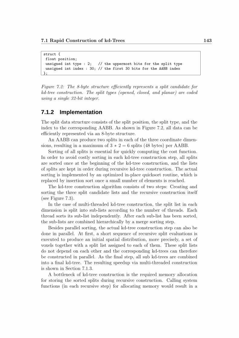
7.1 Rapid Construction of kd-Trees 143
struct {
float position;
unsigned int type : 2; // the uppermost bits for the split type
unsigned int index : 30; // the first 30 bits for the AABB index
};
Figure 7.2: The 8-byte structure efficiently represents a split candidate forkd-tree construction. The split types (opened, closed, and planar) are codedusing a single 32-bit integer.
7.1.2 Implementation
The split data structure consists of the split position, the split type, and theindex to the corresponding AABB. As shown in Figure 7.2, all data can beefficiently represented via an 8-byte structure.
An AABB can produce two splits in each of the three coordinate dimen-sions, resulting in a maximum of 3 ∗ 2 = 6 splits (48 bytes) per AABB.
Sorting of all splits is essential for quickly computing the cost function.In order to avoid costly sorting in each kd-tree construction step, all splitsare sorted once at the beginning of the kd-tree construction, and the listsof splits are kept in order during recursive kd-tree construction. The actualsorting is implemented by an optimized in-place quicksort routine, which isreplaced by insertion sort once a small number of elements is reached.
The kd-tree construction algorithm consists of two steps: Creating andsorting the three split candidate lists and the recursive construction itself(see Figure 7.3).
In the case of multi-threaded kd-tree construction, the split list in eachdimension is split into sub-lists according to the number of threads. Eachthread sorts its sub-list independently. After each sub-list has been sorted,the sub-lists are combined hierarchically by a merge sorting step.
Besides parallel sorting, the actual kd-tree construction step can also bedone in parallel. At first, a short sequence of recursive split evaluations isexecuted to produce an initial spatial distribution, more precisely, a set ofvoxels together with a split list assigned to each of them. These split listsdo not depend on each other and the corresponding kd-trees can thereforebe constructed in parallel. As the final step, all sub kd-trees are combinedinto a final kd-tree. The resulting speedup via multi-threaded constructionis shown in Section 7.1.3.
A bottleneck of kd-tree construction is the required memory allocationfor storing the sorted splits during recursive construction. Calling systemfunctions (in each recursive step) for allocating memory would result in a

144 Chapter 7: Dynamic Scenes
————- Preprocessing Step —————empty split candidate lists splx, sply, and splz (index indicates dimension)for all box b in AABB list do
insert split candidates of box b (opened+closed or planar) into split lists splx, sply,and splz
end forsort each split candidate list splx, sply and splz according to split position
——– Recursive KD-Tree Building Code: build(splx, sply,splz) ——-for all split candidate list spl of splx, sply and splz do
#opened = 0 // number of opened splits#closed = 0 // number of closed splits#planar = 0 // number of planar splitsfor all split candidate s of split candidate list spl do
increase #opened, #closed, or #planar according to split type of s
eval cost function cost(x) for s according to #opened, #closed, and #planar
if cost(s) < cost(bestsplit) thenbestsplit = s
end ifend for
end forif cost(bestsplit) < COST FOR LEAF then
for all split candidate list spl of splx, sply and splz dosplit spl according to bestsplit into two splleft and splright
end forbuild(splleft−x, splleft−y,splleft−z) // continue recursivelybuild(splright−x, splright−y, splright−z) // continue recursively
elsecreate leaf
end if
Figure 7.3: Rapid kd-tree construction algorithm based on axis-aligned bound-ing boxes. The algorithm basically consists of two steps: Sorting of all po-tential split candidates (required for fast SAH evaluation), and the recursiveconstruction process itself. The ordered split candidate lists allow for per-forming the SAH evaluation of split candidates with linear complexity. Asthe sorting complexity is O(n log n) (quicksort) and the build complexity isO(n log n), the total complexity of the algorithm is O(n log n).
significant performance drop. Therefore, a carefully written memory poolimplementation, using a certain amount of pre-allocated memory allows forhandling split lists with almost no costly system calls.

7.1 Rapid Construction of kd-Trees 145
0
0.2
0.4
0.6
0.8
1
1.2
0 10000 20000 30000 40000 50000 60000 70000 80000 90000 100000
sec
primitives
Single ThreadTwo Threads
Figure 7.4: kd-tree construction time with an increased number of primitives.Even when using costly surface area heuristics for determining the best splitplane, the highly optimized implementation allows for constructing the kd-tree for 100, 000 primitives in less than half a second when distributing thework among two threads. Note that due to memory caching effects, the multi-threaded construction shows even a superlinear speedup.
7.1.3 Results
An optimized implementation of split sorting, cost function evaluation, splitlist partitioning, and leaf creation makes it possible to construct scenes con-sisting of thousands of primitives within a fraction of a second.
Figure 7.4 shows the construction timings in relation to an increasingnumber of primitives (bicubic Bezier patches). Even with 100, 000 patches,the implementation requires only one second for the complete constructionprocess. When distributing the construction work among two threads (dual-processor PC), a significant reduction of up to 50% can be achieved. Notethat the multi-threaded timings still include thread creation time.
Applying ray-patch intersection that does not require an additional spa-tial index structure per-patch, e.g. an intersection based on uniform refine-

146 Chapter 7: Dynamic Scenes
ment (see Chapter 6), allows for arbitrary dynamic manipulation by simplytransforming the patch control points. In terms of complete Bezier scenes,one simply needs to reconstruct the kd-tree over the corresponding patches.
Figure 7.5: Combining the tracing of ray bundles for Bezier patches with fastkd-tree construction allows for efficiently handling even completely dynamicscenes with arbitrary movement. This scene consists of 144 cones, each coneconsisting of 4 Bezier patches (576 patches in total). The kd-tree over allpatches is rebuilt from scratch for every frame. On a 2.2 GHz Pentium-IV,it runs with 6.6 fps at a resolution of 800 × 600.
Figure 7.4 shows that even kd-tree reconstruction of 20, 000 patches re-quires less than 100 milliseconds. In order to demonstrate this new feature,a waving field (see Figure 7.5) of 12 × 12 = 144 cones was created, which isrebuilt from scratch for every frame. A build time of only a few millisecondsleaves enough time for ray tracing this fully dynamic scene with 6.6 fps on a2.2 GHz Pentium-IV processor.
Apart from completely dynamic scenes, the startup time for highly com-plex scenes can also be significantly reduced. Figure 7.6 shows an artificialcube of 32, 768 teapots. Each teapot consists of 32 patches, correspondingto a total of 1, 048, 576 patches. Even for this huge number of patches, amulti-threaded kd-tree construction makes it possible to achieve an almostimmediate startup time of 4.42 seconds. Thanks to the ray bundle techniquesof Chapter 6, this huge amount of patches can be rendered with 2.5 fps at aresolution of 800 × 600.
Applying the fast kd-tree construction algorithm to triangular scenesshows that the total rendering performance is reduced by about 20−40% com-

7.1 Rapid Construction of kd-Trees 147
Figure 7.6: With coherent ray bundles, even huge scenes of, for example,32, 768 teapots (1, 048, 576 patches) can be interactively ray traced at 2 fpsat a resolution of 800 × 600 on a 2.2 GHz Pentium-IV. With multi-threadedkd-tree construction the startup time for this scene is reduced to less than 5seconds.
pared to high-quality triangular-based kd-tree construction [Wald04]. How-ever, compared to the construction time of the high-quality kd-tree, a 10to 20 times faster construction is achieved, even when using only the singlethreaded version. As for Bezier patches, the fast kd-tree construction makesit possible to ray trace fully dynamic scenes of several thousand triangles.
Analyzing the fast kd-tree construction code using profiling tools such asVTune [Intel04] shows that for an increasing number of primitives (measuredfrom 16, 384 to 1, 040, 576), the sorting of split candidates takes up 30% to35% of the total construction time.
As shown in Figure 7.4, the construction time is almost linear in thenumber of primitives. Usually, one would expect an increase in constructiontime if the working set becomes larger than the L2 cache size. However, evenwith hundreds of thousands of primitives, the major amount of the workingset can be held in the CPU cache hierarchy. Moreover, the working set canbe loaded very quickly into the cache hierarchy because the sequential accesspattern of SAH evaluation and split sorting is very suitable for the built-inhardware memory prefetcher.
The actual bottlenecks of the code (measured by VTune) are located inthe evaluation of the SAH and the sorting of splits according to the chosensplit candidate. As a split is a compound data type (position and type),

148 Chapter 7: Dynamic Scenes
a split comparison typically performs multiple branches. Therefore, splitsorting involves a large number of mis-predicted branches. In terms of furtheroptimization, one has to lower the amount of mis-predicted branches first.Removing branches by Boolean expressions might be a good solution to thisproblem. Evaluating the SAH for multiple split candidates in parallel usingSIMD instructions could further reduce the number of mis-predicted branchesand additionally increase the SAH split evaluation throughput. As a result,further low-level code optimizations could provide a significant speedup ofperformance.
7.2 Conclusions and Future Work
Multi-core CPUs will make it possible to efficiently construct kd-trees usingmultiple threads. The current implementation already supports two threads,where both of them are used for the split sorting step and the constructionprocess. For the latter, the two threads start working independently oncethe split candidate list has been sorted according to the first chosen splitcandidate. In the case of multiple threads, the split candidate lists have tobe sorted multiple times in order to provide a working set for each thread.
The time for generating the working sets might be further reduced byusing either a hierarchical startup, where one thread starts two sub-threads,or an initial spatial sorting. A regular grid structure could be used as initialspatial sorting, permitting the sorting step to be performed very quickly.The number of non-empty grid cells would correspond to the initial numberof working sets, which can be directly assigned to the set of constructionthreads.
Obviously, not all objects have to be reconstructed for every frame. Ifno ray accesses the object, the spatial index structure does not need to berebuilt. In the case a ray accesses the bounding box of an object, a simple testcould be performed if the index structure has already been built. Moreover,the rapid kd-tree construction algorithm could also be used for adaptive kd-tree construction [Havran01]. The idea behind adaptive kd-tree constructionis to build the kd-tree on the fly during ray traversal. The more rays hit agiven object, the finer the corresponding kd-tree must be built.

Chapter 8
Distributed Coherent RayTracing on Clusters
8.1 Introduction
Even though the compute power of a single or dual-processor workstation isquite sufficient for realizing interactive ray tracing with a small number ofrays per pixel and simple shading, it is not enough for high frame rates incombination with many advanced shading effects.
In order to compensate for the need of compute power, researchers haveused large shared-memory supercomputers (all processors share the samemain memory) with up to hundreds of processors. Such a hardware setup hasallowed for “pushing” ray tracing performance to realtime level rates [Keates95,Muuss95a, Muuss95b, Parker99b, Parker98, Parker99a], but the cost for ahigh-end supercomputer is tremendous. Because of the cost, these high-endsystems are not very common.
On the “low-end” side, multi-processor systems [Intel01, AMD03, IBM05]with more than two processors (or cores) are not standard and thereforeexpensive. Even though this is beginning to change, arbitrarily increasingthe number of processors within an off-the-shelf PC is often not possible. Asthe processor and the supporting hardware have to be exclusively designed formulti-processing, “low-end” multi-processor systems are typically restrictedto a small number of CPUs. Unfortunately, the quality and complexityrequirements of advanced ray tracing-based rendering algorithms can easilysaturate the available compute power of small multi-processor systems.
Given the requirements of ray tracing, there is a tremendous need for aneasy and inexpensive way to combine the compute power of several smallsingle or multi-processor systems. In order to keep costs low, the method

150 Chapter 8: Distributed Coherent Ray Tracing on Clusters
of choice would be to connect the different systems by inexpensive off-the-shelf network technology. Unfortunately, this makes things more complicatedbecause the total system would then be a distributed memory system (eachdesktop PC can only access its own main memory), and the interconnectionframework for transferring data between the system’s components suffersfrom a low bandwidth and a high latency. In order to compensate for this,a distribution framework is required that is able to handle the impacts of adistributed memory environment and high latency communication [Wald02a,Dietrich03, DeMarle03, Wald04, DeMarle04].
This chapter will provide a detailed presentation of the distribution frame-work that is used within the OpenRT library [Wald02a, Dietrich03, Wald04].The framework has been exclusively designed for efficiently combining thecompute power of a cluster of PCs, while handling all related memory andinterconnection issues.
Before giving details about the OpenRT distribution framework, a briefoverview of distribution strategies for parallel ray tracing will be presentedfirst. Note that in the following a set of standard desktop PCs is referred asa cluster of rendering nodes.
8.2 Distribution Strategies
The main task for parallel ray tracing is to define a set of tasks that can bedistributed across processors and executed in parallel. The preferable way forachieving the best performance is to split up the most time-consuming partof the rendering algorithm into independent tasks which can be executed inparallel. In terms of ray tracing, this typically means the shooting of rays.
In the following, a brief overview of typical tasks used for parallel raytracing [Reinhard97, Reinhard95, Chalmers98, Chalmers01] is given:
Frame Distribution: In the context of off-line rendering, the tasks are typ-ically defined as complete frames. Distributing frames across a renderfarm allows for achieving a high frame throughput, but the costs forrendering one frame are more or less constant.
Scene Subdivision: The scene data is partitioned by spatial subdivision.The resulting scene parts are distributed across the nodes of a dis-tributed memory system. Based on the spatial location within thescene, the rays are transferred during traversal between the differentsystem elements. This approach allows for rendering highly complexscenes that exceed the main memory of a single PC, since each systemelement handles only a fraction of the complete scene data. On the

8.2 Distribution Strategies 151
other hand, rays must be reordered (based on their location) and allray data has to be transferred across the network.
Image Subdivision: Due to the fact that the color of each pixel can be com-puted independently of any other pixel, a distribution strategy basedon image plane subdivision can be used to speedup the rendering of asingle frame. In order to display the final frame, only the computedpixel colors need to be combined.
Looking at the distribution schemes in detail makes it clear that not all ofthem are suitable for realtime ray tracing on a distributed memory system.A frame-based distribution would introduce a latency corresponding to theamount of time required for rendering all distributed frames. For a realtimesystem requiring immediate feedback, the approach is not acceptable.
On the other hand, scene subdivision is also sub-optimal because thelimited bandwidth of the interconnection framework makes it difficult totransfer data quickly. As rays typically traverse large spatial regions, manydifferent spatial locations are accessed. Therefore, a huge amount of raydata must be transferred between nodes. Representing a ray usually requiresat least 32 bytes (direction, origin, intersection distance, primitive id) andassuming a resolution of 1024× 1024 pixels and 10 rays per pixel, yields 320MB per frame. This amount of data simply exceeds the bandwidth of today’sinterconnection techniques.
Additionally, the connection of spatial locations to nodes typically creates“hot spots” during ray traversal, because most of the time only a few nodesactually work in parallel. For example, the nodes containing the camera orthe light sources will need to handle numerous rays, thereby becoming “hotspots”. Due to this sub-optimal utilization and the consequently limitedscalability, the OpenRT framework instead uses image plane subdivision fortask distribution.
A typical image-based distribution approach relies on individual pixels.For example pixel i would be assigned to node i mod n, where n is thenumber of nodes. Even though the required transfer of pixel coordinates andcolors would require less bandwidth than sending ray data, the amount is stillsignificant. Assuming two bytes per pixel coordinate yields 4 MB, withoutthe actual pixel colors for a resolution of 1024 × 1024 pixels. Additionally,relying on individual pixels complicates the gathering of coherent primaryray bundles because of the spacing between pixels assigned to a particularnode.
Given bandwidth requirements, a distribution scheme with an imageplane subdivided into rectangular tiles is more beneficial. Rectangular tiles
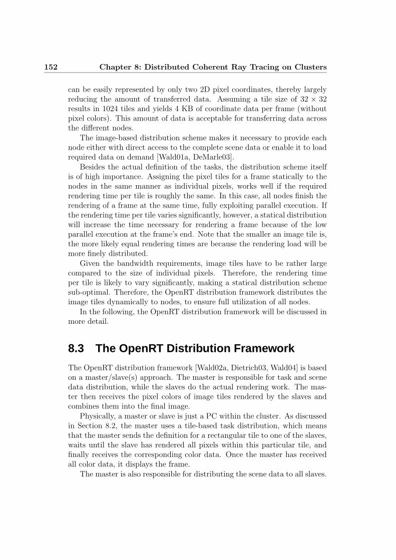
152 Chapter 8: Distributed Coherent Ray Tracing on Clusters
can be easily represented by only two 2D pixel coordinates, thereby largelyreducing the amount of transferred data. Assuming a tile size of 32 × 32results in 1024 tiles and yields 4 KB of coordinate data per frame (withoutpixel colors). This amount of data is acceptable for transferring data acrossthe different nodes.
The image-based distribution scheme makes it necessary to provide eachnode either with direct access to the complete scene data or enable it to loadrequired data on demand [Wald01a, DeMarle03].
Besides the actual definition of the tasks, the distribution scheme itselfis of high importance. Assigning the pixel tiles for a frame statically to thenodes in the same manner as individual pixels, works well if the requiredrendering time per tile is roughly the same. In this case, all nodes finish therendering of a frame at the same time, fully exploiting parallel execution. Ifthe rendering time per tile varies significantly, however, a statical distributionwill increase the time necessary for rendering a frame because of the lowparallel execution at the frame’s end. Note that the smaller an image tile is,the more likely equal rendering times are because the rendering load will bemore finely distributed.
Given the bandwidth requirements, image tiles have to be rather largecompared to the size of individual pixels. Therefore, the rendering timeper tile is likely to vary significantly, making a statical distribution schemesub-optimal. Therefore, the OpenRT distribution framework distributes theimage tiles dynamically to nodes, to ensure full utilization of all nodes.
In the following, the OpenRT distribution framework will be discussed inmore detail.
8.3 The OpenRT Distribution Framework
The OpenRT distribution framework [Wald02a, Dietrich03, Wald04] is basedon a master/slave(s) approach. The master is responsible for task and scenedata distribution, while the slaves do the actual rendering work. The mas-ter then receives the pixel colors of image tiles rendered by the slaves andcombines them into the final image.
Physically, a master or slave is just a PC within the cluster. As discussedin Section 8.2, the master uses a tile-based task distribution, which meansthat the master sends the definition for a rectangular tile to one of the slaves,waits until the slave has rendered all pixels within this particular tile, andfinally receives the corresponding color data. Once the master has receivedall color data, it displays the frame.
The master is also responsible for distributing the scene data to all slaves.

8.3 The OpenRT Distribution Framework 153
The same holds true for scene data updates, e.g. a new camera or light sourceposition, which are once more transferred from the master to all slaves. Notethat this transfer is unidirectional, as there is no need for transferring scenedata from slave to master. For the OpenRT framework, there is no differ-ence between the initial scene data distribution and subsequent scene dataupdates, because an application communicates with the underlying libraryonly through the OpenRT API. The OpenRT framework distributes eachAPI call, with the exception of geometry calls, to all slaves. This mecha-nism is similar to remote procedure calls, except that OpenRT distributesthe API calls asynchronously. Geometry calls are cached on the master untilthe corresponding object is completely defined. Geometry caching avoids thedistribution of many geometry calls, saving costly bandwidth.
The main issue of the tile-based task distribution is to avoid idle periodson the slave side. These idle periods can have the following reasons:
Communication Latency: When relying on standard network technology,the network round-trip time (master-slave-master) is in the region ofmilliseconds. During such a time span, one could trace thousands ofrays, which means that communication-related dependency chains be-tween master and slave should be avoided or kept to a minimum. If,for example, the master only sends a new task to a slave after havingfirst received the color data of a previous tile, the slave would spend alot of time waiting for the next task.
Synchronization: Parallel execution is always affected by synchronization,because synchronization means serialization. In terms of an image-based ray tracing system, synchronization occurs after the end of framen and before the start of frame n + 1. Only during this period can thescene data be updated (during rendering, it has to be fixed to avoidinconsistent scene data).
The OpenRT framework minimizes these idle periods by introducingasynchronous behavior and special latency hiding techniques:
Dynamic Load Balancing: The scene and shading complexity typicallyvary across the image plane. Therefore, a dynamic load balancingscheme is used. Each slave requests a task (tile) from the master. Iffrequently the rendering of tiles takes longer, the corresponding slavewill ask for work less often, allowing other slaves to take over part ofthe image computation. This ensures that a high variation in renderingtime complexity will be handled more efficiently.

154 Chapter 8: Distributed Coherent Ray Tracing on Clusters
Task Prefetching: In order to hide communication latency on the slaveside when requesting tiles from the master, a fixed number of tiles isassigned to each slave in advance. These tiles are stored on the slaveside in a task queue. By transferring the color data of a computed tileback to the master, the slave simultaneously requests a new tile fromthe master. However, as there still are tasks left in the task queue,the slave can directly continue with the next task without having towait for the arrival of the new one. In order to prevent stalls, the timerequired to render the tiles within the task queue must be greater thanthe round-trip time for sending and receiving a tile.
Asynchronous Data Transfer: Given the limited bandwidth and high la-tency, a transfer of data across the network is costly. The most criticaltime span is required for transferring scene data updates from the mas-ter to the slaves because the master has to broadcast the data. There-fore, asynchronous data transfer has been integrated: While slaves arerendering frame n, the master directly transfers the scene data forframe n + 1 to the slaves. During rendering of frame n, frame n − 1 isdisplayed. This introduces one frame of latency between the renderingand the display of a frame, but gives the master the time span of oneframe to transfer scene data updates to all slaves.
Two-Frames Task Scheduling: Even though dynamic load balancing triesto distribute the rendering task evenly over the slaves, idle periods onthe slaves occur when the master has to synchronize all slaves at theend of a frame. In this case, all tiles of a given frame have been sent,but the corresponding rendering has not been finished yet on the slaveside. Before the master can distribute the tiles of the next frame, ithas to wait until all tiles from the previous frame have been received.In order to prevent idle periods because of frame synchronization, themaster allows the slaves to continue rendering with the next frame(even if the current frame has not yet been completely finished by allslaves). In the event a slave has already received the scene data for thenext frame, it can directly proceed with the rendering (if not, the slavehas to wait until data reception is completed).
Supporting latency hiding techniques requires asynchronous behavior onthe master and the slave side. In the following sections, the master and slaveimplementation used in the OpenRT framework will be presented.
The implementation has been exclusively designed for high-performance.Therefore, no sophisticated library such as MPI [Foruma], PVM [Geist94]was used to prevent abstraction layer overhead in network communication.

8.3 The OpenRT Distribution Framework 155
Instead, the implementation uses a framework that is directly based on thestandard UNIX sockets [Stevens98]. All communication relies on the TCP/IPprotocol. Even though communication based on UDP would offer featuressuch as network broadcast, the possible loss of data would require specialand complex countermeasures. For parallel thread execution, OpenRT relieson the POSIX pthread library [Nichols96].
Tile Receiver
Thread
Tile Render
Thread
Tile Render
Thread
Tile
FIFOTile
FIFO
Master
Tile Sender
Thread
Scene Data
Receiver
Thread
Data
FIFO
Slave
Figure 8.1: Multi-threaded slave implementation: Each colored box corre-sponds to a single thread, a colored circle representing a shared data structure.The green and blue rectangles form the rendering pipeline, which receives im-age tile data over the network from the master, performs the rendering andsends the corresponding pixel colors back to the master. The second pipelinewhich runs asynchronously to the first, receives scene data from the masterover the network, and stores it in the data queue. Once all tiles for the givenframe have been rendered, the rendering threads are synchronized and thescene data is updated based on the content of this queue.
8.3.1 Slave
The slave relies on two asynchronously running pipelines, each consisting ofone or multiple threads (see Figure 8.1). The first pipeline, the so-calledrendering pipeline, is responsible for receiving image tiles from the master,performing the actual rendering, and for sending back the color data to themaster. Each of these three steps is handled by a separate thread.
The “execution flow” for the rendering pipeline is as follows: The TileReceiver Thread is listening on a network socket connected to the master. As
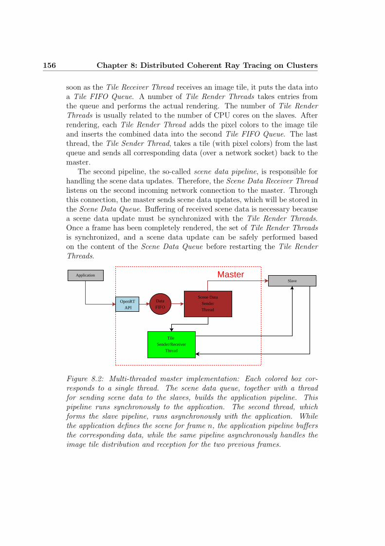
156 Chapter 8: Distributed Coherent Ray Tracing on Clusters
soon as the Tile Receiver Thread receives an image tile, it puts the data intoa Tile FIFO Queue. A number of Tile Render Threads takes entries fromthe queue and performs the actual rendering. The number of Tile RenderThreads is usually related to the number of CPU cores on the slaves. Afterrendering, each Tile Render Thread adds the pixel colors to the image tileand inserts the combined data into the second Tile FIFO Queue. The lastthread, the Tile Sender Thread, takes a tile (with pixel colors) from the lastqueue and sends all corresponding data (over a network socket) back to themaster.
The second pipeline, the so-called scene data pipeline, is responsible forhandling the scene data updates. Therefore, the Scene Data Receiver Threadlistens on the second incoming network connection to the master. Throughthis connection, the master sends scene data updates, which will be stored inthe Scene Data Queue. Buffering of received scene data is necessary becausea scene data update must be synchronized with the Tile Render Threads.Once a frame has been completely rendered, the set of Tile Render Threadsis synchronized, and a scene data update can be safely performed basedon the content of the Scene Data Queue before restarting the Tile RenderThreads.
Master
Tile
Sender/Receiver
Thread
Scene Data
Sender
Thread
Application
Slave
Data
FIFOOpenRT
API
Figure 8.2: Multi-threaded master implementation: Each colored box cor-responds to a single thread. The scene data queue, together with a threadfor sending scene data to the slaves, builds the application pipeline. Thispipeline runs synchronously to the application. The second thread, whichforms the slave pipeline, runs asynchronously with the application. Whilethe application defines the scene for frame n, the application pipeline buffersthe corresponding data, while the same pipeline asynchronously handles theimage tile distribution and reception for the two previous frames.
8.4 Communication and Dataflow 157
8.3.2 Master
Similar to the slave, the master consists of two asynchronously runningpipelines (see Figure 8.2). The first pipeline, the so-called application pipeline,runs synchronously with the application, whereas the second pipeline, theslave pipeline, runs asynchronously to the application.
The main task of the application pipeline is to distribute scene data up-dates (in the form of OpenRT API calls) over the network to all slaves. Thepoint in time when all scene data for the current frame is defined, is also thepoint of synchronization with the second pipeline. At the synchronizationpoint, the application pipeline waits until all pixel data for a new frame hasbeen received and completely copied to the frame buffer.
The slave pipeline consists of a single thread, called Tile Sender/ReceiverThread, which handles all tile-based communication between master andslaves. It listens on the network sockets which connect the master to theslaves. It responds to each incoming tile color data with a new tile task.If all tile tasks for the current frame have already been assigned, tiles forthe next frame are used. Therefore, tiles for a maximum of two frames canbe in-flight. As a result, the Tile Sender/Receiver Thread must be capableof handling tiles for two different frames at the same time, which directlytranslates to supporting double-buffering via two internal frame buffers.
8.4 Communication and Dataflow
For a better understanding of the asynchronous behavior of master and slave,a simplified timing diagram is shown in Figure 8.3.
While the master receives all tile data for frame n, frame n−1 is displayed.The master’s application pipeline is locked until all tiles for frame n have beenreceived. At this point, the lock for the application pipeline is released, andframe n can be displayed by the application. Moreover, the application canalready start to specify the scene for frame n + 1.
Due to an one-to-one exchange of color data and new tasks, the master hasto distribute tiles for frame n+1 (all tiles for frame n have been distributed),while still waiting for the color data of frame n. This is the key point toprevent idle periods on the slaves, because the master allows those slaves toproceed with the rendering of frame n + 1 which have already received thescene data for frame n + 1.
The slave receives, renders, and sends back tile data for frame n, whileasynchronously receiving the data for frame n + 1. When all scene datafor frame n + 1 has been received, the slave updates the scene data by the

158 Chapter 8: Distributed Coherent Ray Tracing on Clusters
Display
Master (App)
Master (Tile)
Slave (Data)
Frame n-2
S Tiles Frame n-1
S Data Frame n
Slave (Receive)
Slave (Render)
Slave (Send)
R Tiles Frame n-1
R Tiles Frame n-1
RD Tiles Frame n-1
S Tiles Frame n-1
R Data Frame n
U Data Frame n
Frame n-1
S Data Frame n+1
S Tiles Frame n
R Tiles Frame n
R Data Frame n+1
RD Tiles Frame n
S Tiles Frame n
R Tiles Frame n
Frame n
S Data Frame n+2
S Tiles Frame n+1
R Tiles Frame n+1
R Data Frame n+2
R Tiles Frame n+1
U Data Frame n+1
RD Tiles Frame n+1
S Tiles Frame n+1
Figure 8.3: The timing diagram for master-slave communication (S = Send,R = Receive, U = Update, RD = Render). The main synchronization pointappears when all tiles for frame n have been received. Only at this point is theapplication able to display frame n. While distributing tile jobs and receivingcolor data back for frame n, the master sends data for frame n + 1 to allslaves. The slave asynchronously buffers this data, while it receives, renders,and sends data for frame n. Therefore, one frame of latency between thespecification and display of a frame is introduced.
buffered data, while the master is still waiting for color data of the previousframe. As long as all scene data is received before the rendering of the lastimage tile is finished, the time for the network transfer can be completelyhidden. If the time required for updating the scene data is sufficiently small,the slave will have almost no idle periods in terms of rendering. Between thespecification and the display of a frame, one frame of latency is introduced.
In the case of using multiple rendering threads, the update must onlybe executed by a single thread. Therefore, all rendering threads need to beserialized at this point.
As discussed in Section 8.3, the master distributes a set of tiles in advance.

8.5 Results 159
These tiles are directly buffered by a Tile FIFO Queue, so that they can bedirectly requested by a rendering thread. If the master receives the color datafor the first tile of the set, it will send a new tile. In the case of n renderingthreads, the time required for rendering all tiles in the queue decreases to1/n of the original time span. Therefore, the number of tiles sent in advancemust be increased accordingly.
8.5 Results
For testing the scalability of the master/slave distribution framework, a clus-ter of 24 dual Athlon MP 1800+ (48 CPUs in total) with 512 MB memorywas used. For each CPU, a separate slave process was created, yielding amaximum of 48 slaves running simultaneously.
Since all slaves transfer the image data to the master, the network band-width to the master can easily become a bottleneck. Therefore, the slavePCs are interconnected by a fully switched 100Mbit Ethernet using a Giga-bit uplink to the master.
A set of four triangular example scenes was rendered at a resolution of640 × 480, using only primary rays and simple shading. The scene com-plexity ranged from a few thousand triangles for the “Office” scene up toseveral millions for the “Power Plant” scene. For a detailed scene descriptionsee [Wald03e, Wald04].
Figure 8.4 shows that for all example scenes the distribution frameworkachieves linear scalability in the number of CPUs (slaves) until the networkbandwidth to the master is saturated. For the given setup, the saturationappears when more than 22 MB/s have to be transferred over the network.For a resolution of 640 × 480 and color coding of three bytes per pixel,this corresponds to a maximum of 25 frames per second. By combiningthe bandwidths of several Gigabit network connections, the framework evenallows for reaching 40 − 50 fps.
8.6 Conclusions and Future Work
The proposed master/slave-based distribution framework allows for efficientlycombining the compute power of several PCs interconnected by standard net-work technology. The framework has been designed especially for scalabilityand interactivity, while relying on a high-latency interconnection. In orderto hide the interconnection latency, several techniques such as dynamic load-balancing, task scheduling, task prefetching and asynchronous data transfer

160 Chapter 8: Distributed Coherent Ray Tracing on Clusters
0
5
10
15
20
484032241681
frames per second
CPUs
OfficeHeadlight
Power PlantSunflowers
Figure 8.4: Scalability of the master/slave distribution framework for an in-creasing number of CPUs (slaves) and different example scenes. All sceneshave been rendered at a resolution of 640 × 480 using only primary rays andsimple shading. The complexity of scenes ranges from a few thousand trian-gles for the Office scene up to several million triangles for the Power Plantscene. For all scenes, the distribution framework achieves linear scalabilityin the slaves until the network bandwidth to the master is saturated. Thesaturation appears for the given hardware setup at a maximum transfer rateof 22 MB/s, which corresponds to 25 fps.
have been integrated into the framework. These techniques allow for achiev-ing a linear scalability in the number of connected PCs.
Even though the distribution framework provides linear scalability, themaximum frame rate is limited by the maximum network bandwidth. Forthe network setup shown in Section 8.5, a maximum of 25 frames per sec-ond can be achieved. For future setups, it will be necessary to further in-crease the bandwidth to the master. Obviously, faster network technologylike Myrinet [Forumb] or Infiniband [Futral01], could provide a higher band-width but the required network hardware is still non-standard and thus ex-pensive. Therefore, it might be beneficial to rather focus on fast compression
8.6 Conclusions and Future Work 161
and decompression algorithms in order to reduce the amount of transferreddata. For multi-core CPUs, in particular, one could reserve a single core forcompressing/decompressing pixel data.
In the current implementation, specific system parameters such as the sizeof a pixel tile or the numbers of tiles that a slave fetches in advance are fixed.This typically works well for most situations, while it can be sub-optimalin others. Therefore, future implementations should automatically analyzethe efficiency of the applied parameters by, for example, measuring the loadon the slaves and, if required, adapting these parameters during run-time toensure an optimal work distribution.

162 Chapter 8: Distributed Coherent Ray Tracing on Clusters

Chapter 9
Applications
A key point for achieving high ray tracing performance is ray coherence. Asdiscussed in Section 4.4.5, most of the ray tracing-based rendering algorithms,e.g. standard backward ray tracing, rely on the recursive evaluation of singleray paths. The recursive evaluation makes it difficult to combine individualrays to ray bundles. Even if individual rays can be combined, it is not ensuredthat the rays within the bundle are coherent. Unfortunately, this also appliesfor any other ray-path generating rendering algorithm.
Solving this problem requires a shift in design: Instead of trying to gathercoherent rays out of an arbitrary rendering algorithm, one should design, ormodify, the rendering algorithm in order to produce coherent rays.
In the following section, a rendering algorithm is presented that is able toalmost exclusively produce coherent ray bundles. This rendering algorithmis known as the instant global illumination algorithm, and was originallypresented by Wald et al. [Wald02b, Wald04]. By having a fast ray tracingcore combined with a lot of processing power, the algorithm is able to fullyrecompute a complete global illumination for every frame. The improvedalgorithm [Benthin03] described in this chapter has been designed to fullyexploit coherent ray bundles and to eliminate the bottlenecks of the previousalgorithm [Benthin03].
9.1 Instant Global Illumination
This section briefly reviews the original instant global illumination algorithm.For a more detailed description of this algorithm and other global illumina-tion algorithms see [Wald04].
The core of the instant global illumination algorithm is build on the in-stant radiosity algorithm proposed by Keller et al. [Keller97]. Instant radios-

164 Chapter 9: Applications
ity approximates diffuse illumination by a set of virtual point light sources(VPLs). These VPLs are computed in a preprocessing step by generatinglight paths (using random walks) from the light sources into the scene. Ateach light path bounce, a VPL is created (the emittance of the virtual pointcorresponds to the reflected radiosity at the given point). The contributionof all VPLs approximates the indirect illumination.
The set of VPLs is used in the actual rendering process to compute theirradiance at every point. For each primary ray intersection point, the ir-radiance is computed by shooting shadow rays towards all generated VPLsand adding their contributions. Obviously, the more VPLs are consideredper intersection point, the more accurate the illumination computation willbe. However, as the focus is on interactivity, only a small set of VPLs isaffordable per pixel.
VPLs cause discretization errors due to the generation of sharp shadowboundaries. However, these can be smoothed by using interleaved sam-pling [Keller01]. The idea behind interleaved sampling is to not generateand use only one set of VPLs for all pixels but to generate multiple VPLsets and interleave these sets for the illumination computation of neighbor-ing pixels. An N × N pixel pattern implies the generation of N × N VPLsets. As neighboring pixels do not share the same VPL set, hard shadowboundaries are broken up. All VPL sets are of equal size and, therefore,the number of shadow rays per pixel is similar to the one-set case. Thisimplies that no additional work has to be done. The drawback of interleavedsampling is the transfer of discretization errors into visible structured noise.The combination of interleaved sampling and instant radiosity is illustratedin Figure 9.1.
The structured noise introduced by interleaved sampling can be signifi-cantly reduced by a technique which is called discontinuity buffering [Keller01,Wald02b, Wald04]. Discontinuity buffering essentially filters the irradianceof neighboring pixels. In order to filter over all different VPL sets, the fil-ter kernel must have the same size (N × N) as the interleaved samplingpattern. Discontinuities, e.g. surface edges or cured surfaces must not befiltered, otherwise visible blurring artifacts will appear. Therefore, disconti-nuity buffering relies on several heuristics (hit point distance, surface normal)to detect such cases. The key point of discontinuity buffering is that it al-lows for combining the illumination computation of neighboring pixels. Foran N × N interleaved sampling pattern and an N × N filter kernel, everypixel exploits the illumination from all N × N VPL sets. The combinationof interleaved sampling and discontinuity buffering trades spatial blurringof the illumination for the speed of computation. Usually, the results areacceptable because indirect illumination changes only slowly on surfaces.

9.2 Exploiting Coherence 165
Figure 9.1: Combination of instant radiosity and interleaved sampling:Neighboring pixels use a different set of virtual point lights (VPLs). Thestructured noise introduced by the different VPL sets is on removed later onby filtering the irradiance of neighboring pixels.
9.2 Exploiting Coherence
The standard approach of combining rays from neighboring pixels to coherent(shadow) ray bundles as shown in Chapter 4 does not work any longer whenusing interleaved sampling. Therefore, only pixels that share a commonVPL set produce shadow rays which are coherent. As a result, only thoserays should be combined into bundles. One could trace primary rays fromneighboring pixels together and later reorder the intersection points accordingto the different VPL sets. However, reordering would require many scatter-gather operations, which are costly when using SSE instructions.
Fortunately, reordering is not necessary because an N × N interleavedsampling pattern ensures that every N th pixel (with respect to both rows andcolumns) has the same interleaved sampling index i, 0 ≤ i ≤ N ×N . If N issmall, e.g. 3, grouping primary rays according to their interleaved sampling
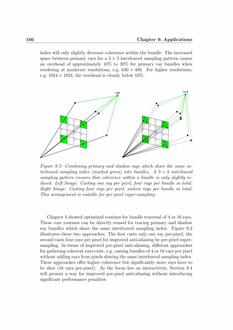
166 Chapter 9: Applications
index will only slightly decrease coherence within the bundle. The increasedspace between primary rays for a 3 × 3 interleaved sampling pattern causesan overhead of approximately 10% to 20% for primary ray bundles whenrendering at moderate resolutions, e.g. 640 × 480. For higher resolutions,e.g. 1024 × 1024, the overhead is clearly below 10%.
12
03
45
367
86
01
20
x
x
x
x
x
VPL
0xxx
x
xxx
x
xxx
x
xxx
x
12
03
45
367
86
01
20
0
VLP
Figure 9.2: Combining primary and shadow rays which share the same in-terleaved sampling index (marked green) into bundles. A 3 × 3 interleavedsampling pattern ensures that coherence within a bundle is only slightly re-duced. Left Image: Casting one ray per pixel, four rays per bundle in total.Right Image: Casting four rays per pixel, sixteen rays per bundle in total.This arrangement is suitable for per-pixel super-sampling.
Chapter 4 showed optimized routines for bundle traversal of 4 or 16 rays.These core routines can be directly reused for tracing primary and shadowray bundles which share the same interleaved sampling index. Figure 9.2illustrates these two approaches: The first casts only one ray per-pixel, thesecond casts four rays per pixel for improved anti-aliasing by per-pixel super-sampling. In terms of improved per-pixel anti-aliasing, different approachesfor gathering coherent rays exist, e.g. casting bundles of 4 or 16 rays per pixelwithout adding rays from pixels sharing the same interleaved sampling index.These approaches offer higher coherence but significantly more rays have tobe shot (16 rays per-pixel). As the focus lies on interactivity, Section 9.4will present a way for improved per-pixel anti-aliasing without introducingsignificant performance penalties.
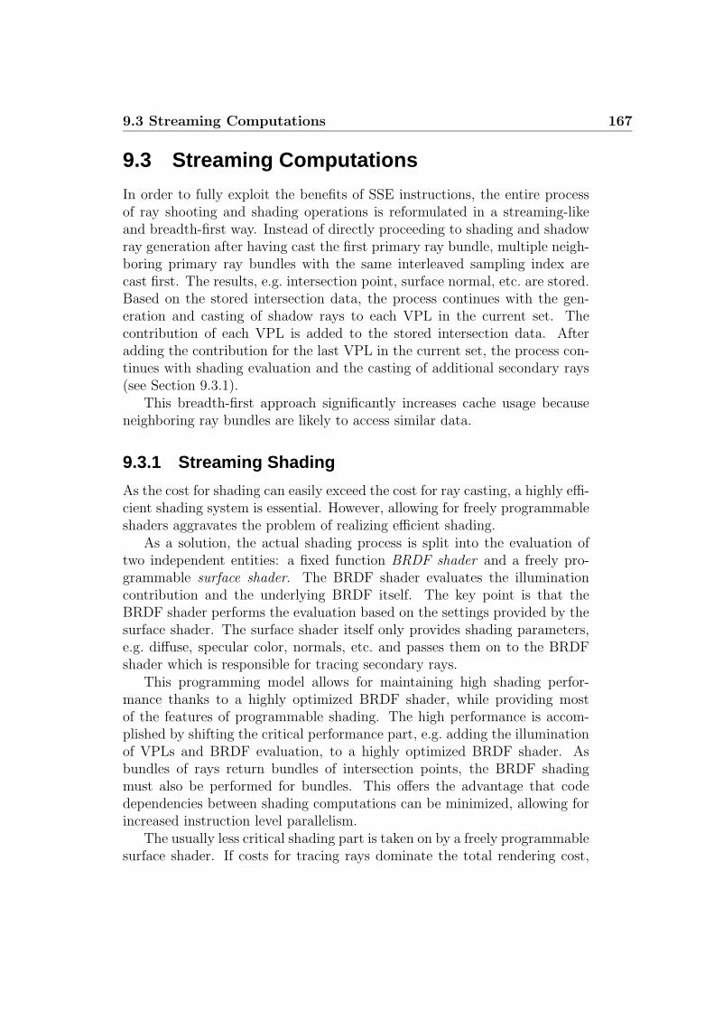
9.3 Streaming Computations 167
9.3 Streaming Computations
In order to fully exploit the benefits of SSE instructions, the entire processof ray shooting and shading operations is reformulated in a streaming-likeand breadth-first way. Instead of directly proceeding to shading and shadowray generation after having cast the first primary ray bundle, multiple neigh-boring primary ray bundles with the same interleaved sampling index arecast first. The results, e.g. intersection point, surface normal, etc. are stored.Based on the stored intersection data, the process continues with the gen-eration and casting of shadow rays to each VPL in the current set. Thecontribution of each VPL is added to the stored intersection data. Afteradding the contribution for the last VPL in the current set, the process con-tinues with shading evaluation and the casting of additional secondary rays(see Section 9.3.1).
This breadth-first approach significantly increases cache usage becauseneighboring ray bundles are likely to access similar data.
9.3.1 Streaming Shading
As the cost for shading can easily exceed the cost for ray casting, a highly effi-cient shading system is essential. However, allowing for freely programmableshaders aggravates the problem of realizing efficient shading.
As a solution, the actual shading process is split into the evaluation oftwo independent entities: a fixed function BRDF shader and a freely pro-grammable surface shader. The BRDF shader evaluates the illuminationcontribution and the underlying BRDF itself. The key point is that theBRDF shader performs the evaluation based on the settings provided by thesurface shader. The surface shader itself only provides shading parameters,e.g. diffuse, specular color, normals, etc. and passes them on to the BRDFshader which is responsible for tracing secondary rays.
This programming model allows for maintaining high shading perfor-mance thanks to a highly optimized BRDF shader, while providing mostof the features of programmable shading. The high performance is accom-plished by shifting the critical performance part, e.g. adding the illuminationof VPLs and BRDF evaluation, to a highly optimized BRDF shader. Asbundles of rays return bundles of intersection points, the BRDF shadingmust also be performed for bundles. This offers the advantage that codedependencies between shading computations can be minimized, allowing forincreased instruction level parallelism.
The usually less critical shading part is taken on by a freely programmablesurface shader. If costs for tracing rays dominate the total rendering cost,

168 Chapter 9: Applications
Figure 9.3: Freely programmable procedural shading in a globally illuminatedscene. The “Shirley 6” test scene (left) in its original form, and after apply-ing several procedural shaders (marble, wood, and brick-bump). The efficientshading model shifts the performance bottleneck towards ray casting. There-fore, even complex and costly shading operations, such as multiple noise func-tion evaluations, only moderately affect total rendering performance. In thiscase, performance drops to 3.7 fps compared to 4.5 fps with constant diffusereflection.
the relative costs for the freely programmable part are relatively low. Thisallows for complex shading operations without large performance penalties(see Figure 9.3).
For standard shading, profiling shows that almost all shading time is takenup by the BRDF shader. This especially applies for adding up the weightedillumination of VPLs: Each VPL in a scene is described by its position xi,the surface normal ni(xi), and its emitted radiance Li. The irradiance at anygiven surface point x with normal n is then approximated by adding up thecontributions from all VPLs:
E(x) =N−1∑
i=0
V (x, xi)cos θx cos θi
||x − xi||2Li, (9.1)
where V (x, y) specifies the visibility between two points x and y, and θx, θi arethe angles between the normal vectors nx, ni and vector x− xi, respectively.Based on the normalized surface and VPL normals, the two cosine factors areevaluated by two dot products, allowing for an efficient SSE implementation.Note that E(x) is evaluated for multiple intersection points in parallel whichallows for efficiently using SSE instructions to perform the dot products. AsVPL normals are normalized before the rendering starts, the normalization
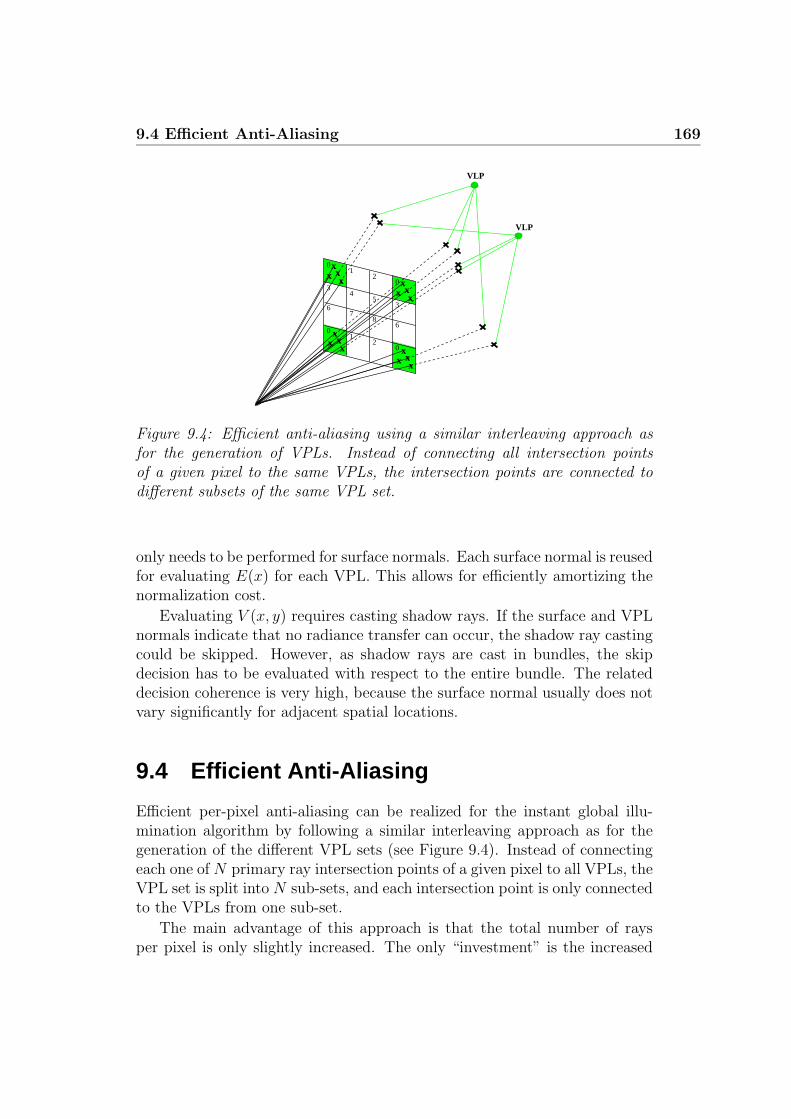
9.4 Efficient Anti-Aliasing 169
xxx
x
xxx
x
xxx
x
xxx
x
12
03
45
367
86
01
20
0
VLP
VLP
Figure 9.4: Efficient anti-aliasing using a similar interleaving approach asfor the generation of VPLs. Instead of connecting all intersection pointsof a given pixel to the same VPLs, the intersection points are connected todifferent subsets of the same VPL set.
only needs to be performed for surface normals. Each surface normal is reusedfor evaluating E(x) for each VPL. This allows for efficiently amortizing thenormalization cost.
Evaluating V (x, y) requires casting shadow rays. If the surface and VPLnormals indicate that no radiance transfer can occur, the shadow ray castingcould be skipped. However, as shadow rays are cast in bundles, the skipdecision has to be evaluated with respect to the entire bundle. The relateddecision coherence is very high, because the surface normal usually does notvary significantly for adjacent spatial locations.
9.4 Efficient Anti-Aliasing
Efficient per-pixel anti-aliasing can be realized for the instant global illu-mination algorithm by following a similar interleaving approach as for thegeneration of the different VPL sets (see Figure 9.4). Instead of connectingeach one of N primary ray intersection points of a given pixel to all VPLs, theVPL set is split into N sub-sets, and each intersection point is only connectedto the VPLs from one sub-set.
The main advantage of this approach is that the total number of raysper pixel is only slightly increased. The only “investment” is the increased

170 Chapter 9: Applications
number of primary rays per pixel while the number of shadow rays remainsconstant. Depending on the size of the VPL set, the performance impactof efficient anti-aliasing typically lies in the range of 10% to 30%, while theactual image quality is significantly enhanced (see Figure 9.5). Differentprimary rays for the same pixel obtain illumination from different VPLs;a possible difference in the illumination is therefore possible (compared toconnecting each primary ray to the same VPL set). In most cases, how-ever, each primary ray is connected to multiple VPLs, thereby reducing theprobability of illumination discrepancies. For typical scenes, the differencein illumination quality is virtually indistinguishable.
Figure 9.5: Left: Casting a single primary ray per pixel exhibits aliasingartifacts for small geometric details. Right: Casting four primary rays perpixel with interleaved shadow ray generation. As the number of shadow raysis constant, performance decreases only from 4 fps to 3.2 fps while providingbetter image quality through anti-aliased rendering.
9.5 Distributed Rendering
High image quality requires many VPLs which in turn requires casting ofmany shadow rays. In order to perform a full recomputation of the completeillumination per frame, the compute power of a single PC is not sufficient. Asa result, multiple PCs need to be combined. The original instant global illu-mination system [Wald02b] as described here therefore uses the distributionframework presented in Section 8.3.
The original instant global illumination system [Wald02b] performs therendering on the slaves and the discontinuity filtering on the master. As a

9.6 Results 171
result, all pixel data required for discontinuity filtering needs to be trans-ferred to the master. The required bandwidth easily saturates the networkbandwidth, thereby limiting the scalability of the entire system. The supportof caustics in the original system makes it necessary to perform the filteringon the master side. By dropping caustics support in the new system, thefiltering step can be moved to the slave side.
A drawback of filtering on the slave side is the overhead caused by thetile-based task distribution system. More precisely, a 3 × 3 filtering kernelrequires access to pixel data which lies outside the tile boundaries. Therefore,the tile has to be virtually enlarged by a one-pixel border. Obviously, thelarger the tile, the smaller the overhead will be. For a tile size of 40 × 40pixels, 164 additional pixels have to be computed. This 10% overhead iseasily acceptable when gaining better scalability in return.
An advantage of filtering on the slave side is that all filtering data canbe completely held in CPU caches. This is beneficial because the filteringstep is then completely memory-bound. As the filter kernel has a regular andfixed size and all input values are provided as single precision floating pointvalues, the actual filtering is efficiently implemented using SSE instructions.If all input values are directly loaded from cache, the SSE-based filter easilyoutperforms a non-SSE version by a factor of about 3.
9.6 Results
The new instant global illumination system [Benthin03] demonstrates theeffectiveness of directly supporting coherent ray bundles using rendering al-gorithms. Streaming shading and filtering (see Section 9.3.1) shift the criticalcomputational part towards ray casting. Combined with the typical settingof using many VPLs per pixel, the total rendering time is strongly dominatedby ray casting. This allows for directly exploiting the fast traversal code forray bundles from Chapter 4.
Table 9.1 shows a comparison between the original and the new instantglobal illumination system. The original system only supports single raytraversal and no streaming shading. The new system’s support for tracingbundles of rays and streaming shading allows for outperforming the old sys-tem by a factor of 3 − 8. The higher the resolution, the higher coherencewithin the ray bundles and the more beneficial bundle traversal becomes.Note that the statistics for the new system already include the 10% overheadcaused by overlapping at tile boundaries.
Even the compute power of a single PC is sufficient to achieve interactiveframe rates at small resolutions. Table 9.2 shows the actual performance per
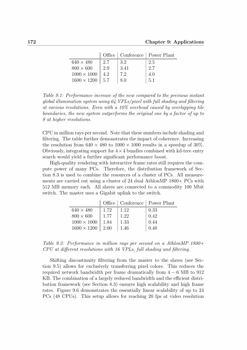
172 Chapter 9: Applications
Office Conference Power Plant
640 × 480 2.7 3.2 2.5800 × 600 2.9 3.41 2.71000 × 1000 4.2 7.2 4.01600 × 1200 5.7 8.0 5.1
Table 9.1: Performance increase of the new compared to the previous instantglobal illumination system using 64 VPLs/pixel with full shading and filteringat various resolutions. Even with a 10% overhead caused by overlapping tileboundaries, the new system outperforms the original one by a factor of up to8 at higher resolutions.
CPU in million rays per second. Note that these numbers include shading andfiltering. The table further demonstrates the impact of coherence. Increasingthe resolution from 640 × 480 to 1000 × 1000 results in a speedup of 30%.Obviously, integrating support for 4×4 bundles combined with kd-tree entrysearch would yield a further significant performance boost.
High-quality rendering with interactive frame rates still requires the com-pute power of many PCs. Therefore, the distribution framework of Sec-tion 8.3 is used to combine the resources of a cluster of PCs. All measure-ments are carried out using a cluster of 24 dual AthlonMP 1800+ PCs with512 MB memory each. All slaves are connected to a commodity 100 Mbitswitch. The master uses a Gigabit uplink to the switch.
Office Conference Power Plant
640 × 480 1.72 1.12 0.33800 × 600 1.77 1.22 0.421000 × 1000 1.84 1.33 0.441600 × 1200 2.00 1.46 0.48
Table 9.2: Performance in million rays per second on a AthlonMP 1800+CPU at different resolutions with 16 VPLs, full shading and filtering.
Shifting discontinuity filtering from the master to the slaves (see Sec-tion 9.5) allows for exclusively transferring pixel colors. This reduces therequired network bandwidth per frame dramatically from 4 − 6 MB to 912KB. The combination of a largely reduced bandwidth and the efficient distri-bution framework (see Section 8.3) ensures high scalability and high framerates. Figure 9.6 demonstrates the essentially linear scalability of up to 24PCs (48 CPUs). This setup allows for reaching 20 fps at video resolution

9.7 Conclusions and Future Work 173
0
5
10
15
20
5 10 15 20
fram
es p
er s
econ
d
slaves
Shirley-6Office
ConferencePower Plant
Figure 9.6: System scalability: Performance is essentially linear for up to 24PCs/48 CPUs. This applies to scenes ranging from several hundred trian-gles (Shirley-6) up to the Power Plant scene with 50 million triangles (fourinstances).
(640 × 480) or 8 fps at full screen resolution (1024 × 1024). Note that evenfor the power plant scene (four instances of 12.5 million triangles each), thecomplete illumination is recomputed from scratch for every single frame (seeFigure 9.7).
9.7 Conclusions and Future Work
Besides adding support for missing illumination effects, e.g. caustics or glossyeffects, it would be a great advance to optimize the system towards multi-core CPUs or shared memory setups. These two hardware setups are alreadybecoming available on the desktop, and will provide enough compute powerto achieve a performance level as the distributed setup. Through linearscalability in the number of processing resources and implicit support forcoherent ray bundles, the instant global illumination system is the methodof choice for realizing interactive global illumination.

174 Chapter 9: Applications
Figure 9.7: Top left: Room with animated globe and lamp, containing roughly20,000 triangles. The lamp illuminates North America which reflects a yel-lowish light into the room. Top right: The globally illuminated conferencescene with 280, 000 triangles and 104 light sources rendering at about 20 fpson 22 dual AthlonMP PCs with 12 VPLs. Center left and right: The well-known Shirley-6 test scene consisting of 600 triangles rendered with proceduralshading. This scene is rendered at roughly 22 fps with 12 VPLs allowing ar-bitrary changes in the scene. Bottom left and right: A power plant scenecontaining four copies of the model with a total of 50 million triangles ren-dered at about 2 fps with global illumination. These two views clearly showthe difference between direct illumination with hard ray traced shadows andthe smooth lighting rendered by the global illumination system. All sceneswere rendered at a resolution of 640 × 480.

Chapter 10
Final Summary, Conclusions,and Future Work
In this final chapter, the content and all new contributions of this thesis willbe briefly summarized. Before concluding, potential future work for all areasdiscussed here will be outlined.
In Chapter 2, the basics of ray tracing and the role of ray tracing asa rendering algorithm were discussed. After defining the core ray tracingalgorithm which forms the basis for ray tracing-based rendering, the factorsthat impact its performance were presented. In particular, the need for anefficient traversal of rays through a spatial index structure and the need foran efficient primitive intersection test were discussed in detail. Based onthis discussion, exploiting coherence, e.g. by traversing coherent ray bundlesand an optimized implementation with respect to the underlying hardwarearchitecture were identified as key factors to improve the performance of thecore ray tracing algorithm.
As optimization in terms of the underlying hardware architecture playsa major role for achieving realtime ray tracing, a detailed discussion of theperformance issues of current CPU architectures, e.g. cache misses, branchmis-predictions, and dependency chains, followed in Chapter 3. Based onthis discussion, coding guidelines which help to achieve optimized code wereproposed next. In addition, the SIMD extension of current CPUs was pro-posed as a powerful tool for exploiting the full compute power of currentCPU architectures.
Chapter 4 used the optimization guidelines of Chapter 3 to describe sev-eral highly optimized example implementations for the traversal of coherentray bundles through a kd-tree. In particular, implementations of differentfrustum traversal algorithms, which allow for constant traversal cost (in terms

176 Chapter 10: Final Summary, Conclusions, and Future Work
of the number of rays within the frustum) were proposed.The efficient ray bundle traversal algorithms presented in Chapter 4 could
be directly used as the basis for ray tracing triangular scenes. Chapter 5 com-bined these traversal algorithms with fast triangle intersection algorithms.By relying on fast traversal and intersection algorithms designed for effi-ciently supporting ray bundles, even interactive ray tracing performance ona single CPU and at high resolutions was achieved.
Chapter 6 showed that interactive ray tracing performance is not limitedto triangular scenes. In particular, highly optimized intersection algorithms,e.g. based on uniform refinement, Bezier clipping, and Newton iteration forefficiently supporting bicubic Bezier surfaces were presented. Each of theseintersection algorithms has its advantages and disadvantages, so choosing aparticular algorithm largely depends on performance and accuracy require-ments.
Chapter 7 showed that the coding guidelines can be efficiently used tooptimize the construction algorithm for high-quality kd-trees. The proposedalgorithm, which even allows for multi-threaded kd-tree construction, is ableto support ray tracing of fully dynamic scenes by reconstructing the corre-sponding kd-tree from scratch for every frame.
The need of ray tracing for compute power can be compensated by com-bining the compute power of multiple PCs. Chapter 8 presented a frame-work for parallel ray tracing using a cluster of off-the-shelf PCs. As theframework was exclusively designed for handling realtime ray tracing on adistributed memory environment, e.g. dealing with high interconnection la-tency and small interconnection bandwidth, linear scalability in the numberof connected PCs was achieved.
Chapter 9 combined several techniques outlined in the preceding chap-ters, e.g. tracing of coherent ray bundles and the distribution framework,in order to realize a system that is even capable of interactively computingglobal illumination. The instant global illumination algorithm presented wasadapted to directly benefit from coherent ray bundles, and extended using ahigh-performance shading framework. Moreover, the proposed implementa-tion of the instant global illumination algorithm in terms of the distributionframework of Chapter 8 allowed for achieving linear performance scalabilityin the number of connected PCs.
Future Work
Even though many aspects of potential future work have already been dis-cussed throughout this thesis, they will be briefly summarized in the following.

177
Extremal traversal of coherent ray bundles allows for constant traversalcost, independently of the number of rays within the bundle. One shouldtherefore concentrate on further reducing the intersection overhead causedby extremal traversal, as compared to that of a standard ray bundle traversalalgorithm. A possible way to achieve this could be to automatically updatethe ray frustum during traversal by excluding already terminated rays.
For triangular scenes, it might be beneficial to store the geometry oftriangles within a leaf as a small index face set. A potential ray bundleintersection would then first perform a side test based on the set of edges.Only for those triangles that fulfill the criteria of the side test, would adistance test be performed in a second step. This algorithm might be ableto avoid a significant amount of unnecessary triangle intersection tests.
In terms of intersection tests for bicubic Bezier surfaces, future optimiza-tions should concentrate on a Newton iteration-based intersection using theKrawczyk operator, because this is the only algorithm that reliably provideshighly accurate results. As the cost and required iterations for the intersec-tion algorithm largely depend on the accurate computation of the intervalextension of the partial derivatives, further optimization should focus on thisoperation. It might also be beneficial to evaluate how the intersection algo-rithm can be efficiently extended to directly support coherent ray bundles.
Besides faster traversal and intersection, efficiently supporting dynamicscenes will be one of the major fields of future research for realtime raytracing. The fast kd-tree construction algorithm proposed in this thesis canbe seen as a first step; supporting scenes as used in today’s computer gameswill require even further optimized algorithms.
Having a system capable of performing realtime ray tracing allows for di-rectly exploring potential ways of realizing realtime global illumination. Themodified instant global illumination algorithm presented in this thesis hasbeen designed to optimally exploit coherent ray bundles. As the algorithmlargely relies on casting shadow rays, future modifications could integrateextremal traversal for efficiently tracing a large number of shadow rays perbundle.
Besides the performance improvements made possible by using better al-gorithms, future hardware architectures will be able to offer an improvedsupport for realtime ray tracing. Instead of increasing performance per CPUby raising the clock speed, future CPU architectures will improve perfor-mance by adding multiple cores to a single CPU chip. Even though currentCPUs have two cores per CPU at the most, all major CPU manufacturershave already announced a higher number of cores for future CPU designs. Ahigh number of cores per CPU is beneficial for ray tracing because the work-load can be distributed across multiple cores. However, multi-core CPUs

178 Chapter 10: Final Summary, Conclusions, and Future Work
present their own problems, e.g. limited interconnection bandwidth betweencores, shared CPU caches, and efficient synchronization techniques. Futurerealtime ray tracing systems must consider these issues to exploit the fullpotential of multi-core CPUs.
A new design in terms of multi-core CPUs was introduced with the CELLprocessor [Cell05]. Instead relying on a homogeneous system of identical CPUcores, the CELL processor has a single standard CPU core and eight addi-tional small CPU cores. These small CPUs have been exclusively designedfor performing SIMD operations. Moreover, each of them has no memorycache but a small amount of local memory attached. If a small CPU corewants to access the main memory, a DMA request must be initiated manually.The new CELL architecture provides a significant amount of SIMD comput-ing power, but requires new programming techniques, because all memorytransfers must be initiated manually. However, a very early prototype im-plementation of a ray tracing system that relied on the algorithms proposedin this thesis was capable of ray tracing the conference scene (tracing onlyprimary rays) with over 30 frames per second at a resolution of 1024 × 1024on a 2.4 GHz CELL processor. Future optimization should concentrate onexploiting the full potential of the CELL chip, which might permit a raytracing system to be created which offers similar compute power as an entirecluster of PCs.
Final Conclusions
This thesis showed that algorithms designed and optimized in terms of theunderlying processor architecture are the key factor for realizing realtime raytracing. Even though for establishing realtime ray tracing as an alternativeto rasterization-based rendering many open questions need to be answeredrealtime ray tracing is already starting to play a major role in 3D graphics.
Through the introduction of powerful multi-core processors, sufficientcompute power will be available on everyone’s desktop to explore the en-tire set of new applications, which now become possible with realtime raytracing.

Appendix A
List of Related Papers
Many parts of this thesis have already been published in previous publica-tions. This chapter provides a list of papers that have contributed to thisthesis and that contain additional information.
2001
Interactive Rendering using Coherent Ray Tracing
Ingo Wald, Carsten Benthin, Markus Wagner, and Philipp SlusallekComputer Graphics Forum, 20(3), 2001, pages 153–164, by A. Chalmersand T.–M. Rhyne (editors), Blackwell Publishers, Oxford, (Proceedingsof Eurographics 2001), Manchester, UK [Wald01c]
Interactive Distributed Ray Tracing of Highly Complex Models
Ingo Wald, Philipp Slusallek, and Carsten BenthinRendering Techniques 2001 (Proceedings of the 12th Eurographics Work-shop on Rendering), by Steven J. Gortler and Karol Myszkowski (edi-tors), pages 274–285, pages 2001, London, UK [Wald01b]
2002
Interactive Global Illumination using Fast Ray Tracing
Ingo Wald, Thomas Kollig, Carsten Benthin, Alexander Keller, PhilippSlusallek , Rendering Techniques 2002, by P. Debevec and S. Gibson(editors) pages 15–24, 2002, Pisa, Italy, (Proceedings of the 13th Eu-rographics Workshop on Rendering) [Wald02b]
180 Chapter A: List of Related Papers
Interactive Headlight Visualization –A Case Study of Interac-
tive Distributed Ray Tracing–
Carsten Benthin, Ingo Wald, Tim Dahmen and Philipp Slusallek, Pro-ceedings of the Fourth Eurographics Workshop on Parallel Graphicsand Visualization (PVG), pages 81–88, Blaubeuren, Germany, 2002[Benthin02]
OpenRT – A Flexible and Scalable Rendering Engine for Inter-
active 3D Graphics
Ingo Wald, Carsten Benthin, and Philipp Slusallek, Technical Report2002, Saarland University Saarbrucken, Germany [Wald02a]
2003
Towards Realtime Ray Tracing – Issues and Potential
Ingo Wald, Carsten Benthin, and Philipp Slusallek, Technical Report2003, Saarland University Saarbrucken, Germany [Wald03d]
The OpenRT Application Programming Interface – Towards A
Common API for Interactive Ray Tracing –
Andreas Dietrich, Ingo Wald, Carsten Benthin, and Philipp Slusallek,OpenSG Symposium 2003, Darmstadt, Germany [Dietrich03]
Interactive Global Illumination in Complex and Highly Oc-
cluded Scenes
Ingo Wald, Carsten Benthin, and Philipp Slusallek, Proceedings of the14th Eurographics Symposium on Rendering, by P. H. Christensen andD. Cohen-Or (editors) pages 74–81, 2003, Leuven, Belgium [Wald03c]
Interactive Distributed Ray Tracing on Commodity PC Clus-
ters – State of the Art and Practical Applications –
Ingo Wald, Carsten Benthin, and Philipp Slusallek, in Harald Kosch,Laszlo Boszormenyi, and Hermann Hellwagner, editors, Euro-Par 2003,Klagenfurt, Austria, volume 2790 of Lecture Notes in Computer Sci-ence, Springer. [Wald03a]
A Scalable Approach to Interactive Global Illumination
Carsten Benthin, Ingo Wald, and Philipp Slusallek, in Computer Graph-ics Forum, 22(3), 2003, pages, 621–630, (Proceedings of Eurographics2003), Granada, Spain [Benthin03]
181
Distributed Interactive Ray Tracing in Dynamic Environments
Ingo Wald, Carsten Benthin, and Philipp Slusallek, SIGGRAPH/EurographicsWorkshop on Parallel Graphics and Visualization (PVG) 2003, Seattle,WA, USA, pages 77-86 [Wald03b]
Realtime Ray Tracing and its Use for Interactive Global Illu-
mination
Ingo Wald, Timothy J.Purcell, Jorg Schmittler, Carsten Benthin, andPhilipp Slusallek, Eurographics 2003 State-of-the-Art Reports, Granada,Spain [Wald03e]
2004
Interactive Ray Tracing of Freeform Surfaces
Carsten Benthin, Ingo Wald, and Philipp Slusallek, Afrigraph 2004,Stellenbosch (Cape Town), South Africa [Benthin04]
2005
A Ray Tracing based Framework for High-Quality Virtual Re-
ality in Industrial Design Applications
Ingo Wald, Carsten Benthin, Alexander Efremov, Tim Dahmen, Jo-hannes Guenther, Andreas Dietrich, Vlastimil Havran, Philipp Slusallek,Hans-Peter Seidel, Technical Report 2005, University of Utah [Wald05]
Techniques for Interactive Ray Tracing of Bezier Surfaces
Carsten Benthin, Ingo Wald, and Philipp Slusallek, Journal of GraphicsTools (to appear) [Benthin05]

182 Chapter A: List of Related Papers

Bibliography
[AltiVec] Motorola Inc. AltiVec Technology Facts. Available athttp://www.motorola.com/AltiVec/facts.html.
[Amanatides87] John Amanatides and Andrew Woo. A Fast Voxel Traver-sal Algorithm for Ray Tracing. In Proceedings of Euro-graphics, pages 3–10. Eurographics Association, 1987.
[AMD03] Advanced Micro Devices. AMD Opteron Processor Model8 Data Sheet. http://www.amd.com/us-en/Processors,2003.
[Arvo87] James Arvo and David Kirk. Fast Ray Tracing by RayClassification. Computer Graphics (Proceedings of ACMSIGGRAPH), 21(4):55–64, 1987.
[Badouel92] Didier Badouel. An Efficient Ray Polygon Intersection.In David Kirk, editor, Graphics Gems III, pages 390–393.Academic Press, 1992.
[Benthin02] Carsten Benthin, Ingo Wald, Tim Dahmen, and PhilippSlusallek. Interactive Headlight Simulation – A CaseStudy of Distributed Interactive Ray Tracing. In Pro-ceedings of the 4th Eurographics Workshop on ParallelGraphics and Visualization (PGV), pages 81–88, 2002.
[Benthin03] Carsten Benthin, Ingo Wald, and Philipp Slusallek. AScalable Approach to Interactive Global Illumination.Computer Graphics Forum (Proceedings of Eurographics),22(3):621–630, 2003.
[Benthin04] Carsten Benthin, Ingo Wald, and Philipp Slusallek. Inter-active Ray Tracing of Free-Form Surfaces. In Proceedingsof Afrigraph, pages 99–106, November 2004.
184 BIBLIOGRAPHY
[Benthin05] Carsten Benthin, Ingo Wald, and Philipp Slusallek. Tech-niques for Interactive Ray Tracing of Bezier Surfaces.Journal of Graphics Tools (to appear), 2005.
[Bittner99] Jiri Bittner. Hierarchical Techniques for VisibilityDetermination. Technical Report DS-005, Depart-ment of Computer Science and Engineering, CzechTechnical University in Prague, 1999. Also avail-able at http:/www.cgg.cvut.cz/∼bittner/publications/-minimum.ps.gz.
[Campagna97] Swen Campagna, Philipp Slusallek, and Hans-Peter Sei-del. Ray Tracing of Parametric Surfaces. The VisualComputer, 13(6):265–282, 1997.
[Cell05] International Business Machines. The Cell Projectat IBM Research. http://www.research.ibm.com/cell/,2005.
[Chalmers98] Alan Chalmers and Erik Reinhard. Parallel and Dis-tributed Photo-Realistic Rendering. In Course notes forACM SIGGRAPH, pages 425–432. ACM Press, 1998.
[Chalmers01] Alan Chalmers, Tim Davis, Toshi Kato, and Erik Rein-hard. Practical Parallel Processing for Today’s RenderingChallenges. In Course notes for ACM SIGGRAPH. ACMPress, 2001.
[Cohen93] Michael F. Cohen and John R. Wallace. Radiosity andRealistic Image Synthesis. Morgan Kaufmann Publishers,1993.
[Cohen94] Daniel Cohen. Voxel Traversal along a 3D Line. In PaulHeckbert, editor, Graphics Gems IV, pages 366–369. Aca-demic Press, 1994.
[Cook84a] Robert Cook, Thomas Porter, and Loren Carpenter. Dis-tributed Ray Tracing. Computer Graphics (Proceeding ofACM SIGGRAPH), 18(3):137–144, 1984.
[Cook84b] Robert L. Cook. Shade trees. Computer Graphics (Pro-ceedings of ACM SIGGRAPH), 18(3):223–231, 1984.

BIBLIOGRAPHY 185
[DeMarle03] David E. DeMarle, Steve Parker, Mark Hartner, Christi-aan Gribble, and Charles Hansen. Distributed InteractiveRay Tracing for Large Volume Visualization. In Proceed-ings of the IEEE Symposium on Parallel and Large-DataVisualization and Graphics (PVG), pages 87–94, 2003.
[DeMarle04] David E. DeMarle, Christiaan Gribble, and StevenParker. Memory-Savvy Distributed Interactive Ray Trac-ing. In Eurographics Symposium on Parallel Graphics andVisualization, pages 93–100, 2004.
[Dietrich03] Andreas Dietrich, Ingo Wald, Carsten Benthin, andPhilipp Slusallek. The OpenRT Application ProgrammingInterface – Towards A Common API for Interactive RayTracing. In Proceedings of the 2003 OpenSG Symposium,pages 23–31, 2003.
[Dietrich05] Andreas Dietrich, Carsten Colditz, Oliver Deussen, andPhilipp Slusallek. Realistic and Interactive Visualizationof High-Density Plant Ecosystems. In Natural Phenom-ena 2005, Proceedings of the Eurographics Workshop onNatural Phenomena, pages 73–81, August 2005.
[Dutre03] Phil Dutre, Philippe Bekaert, and Kavita Bala. AdvancedGlobal Illumination. A K Peters, 1st edition, July 2003.
[Efremov05] Alexander Efremov, Vlastimil Havran, and Hans-PeterSeidel. Robust and Numerically Stable Bezier ClippingMethod for Ray Tracing NURBS Surfaces. In SCCG’05Proceedings, 2005.
[Erickson97] Jeff Erickson. Pluecker Coordinates. Ray Trac-ing News, 1997. http://www.acm.org/tog/resources/-RTNews/html/rtnv10n3.html#art11.
[Farin96] G. Farin. Curves and Surfaces for Computer Aided Geo-metric Design 4th Edition. Academic Press, Boston, 1996.
[Foley97] Foley, van Dam, Feiner, and Hughes. Computer Graphics– Principles and Practice, 2nd edition. Addison Wesley,1997.

186 BIBLIOGRAPHY
[Foley05] Tim Foley and Jeremy Sugerman. KD-tree AccelerationStructures for a GPU Raytracer. In HWWS ’05 Proceed-ings, pages 15–22. ACM Press, 2005.
[Foruma] MPI Forum. MPI – The Message Passing Interface Stan-dard. http://www-unix.mcs.anl.gov/mpi.
[Forumb] Myrinet Forum. Myrinet. http://www.myri.com/-myrinet/overview/.
[Fujimoto86] Akira Fujimoto, Takayuki Tanaka, and Kansei Iwata.ARTS: Accelerated Ray Tracing System. IEEE ComputerGraphics and Applications, 6(4):16–26, 1986.
[Futral01] William T. Futral. Infiniband Architecture: Developmentand Deployment – A Strategic Guide to Server I/O Solu-tions. Intel Press, 2001.
[Geimer05] Markus Geimer and Oliver Abert. Interactive Ray Trac-ing of Trimmed Bicubic Bezier Surfaces without Triangu-lation. In WSCG (Full Papers), pages 71–78, 2005.
[Geist94] Al Geist, Adam Beguelin, Jack Dongarra, WeichengJiang, Robert Manchek, and Vaidyalingam S. Sunderam.PVM: Parallel Virtual Machine. A User’s Guide and Tu-torial for Network Parallel Computing. MIT Press, Cam-bridge, 1994.
[Gigante88] Michael Gigante. Accelerated Ray Tracing using Non-Uniform Grids. In Proceedings of Ausgraph, pages 157–163, 1988.
[Glassner84] Andrew S. Glassner. Space Subdivision For Fast RayTracing. IEEE Computer Graphics and Applications,4(10):15–22, 1984.
[Glassner89] Andrew Glassner. An Introduction to Ray Tracing. Mor-gan Kaufmann, 1989.
[Glassner95] Andrew Glassner. Principles of Digital Image Synthesis.Morgan Kaufmann, 1995.
[GNU] The GNU gcc compiler, version 3.4.X.http://www.gnu.org.

BIBLIOGRAPHY 187
[Goldsmith87] Jeffrey Goldsmith and John Salmon. Automatic Creationof Object Hierarchies for Ray Tracing. IEEE ComputerGraphics and Applications, 7(5):14–20, May 1987.
[Guthe02] M. Guthe, J. Meseth, and R. Klein. Fast and MemoryEfficient View-Dependent Trimmed NURBS Rendering.Pacific Graphics 2002, pages 204–213, October 2002.
[Haines91] Eric Haines. Efficiency Improvements for HierarchyTraversal in Ray Tracing. In James Arvo, editor, GraphicsGems II, pages 267–272. Academic Press, 1991.
[Havran01] Vlastimil Havran. Heuristic Ray Shooting Algorithms.PhD thesis, Faculty of Electrical Engineering, CzechTechnical University in Prague, 2001.
[Hsiung92] Ping-Kang Hsiung and Robert H. Thibadeau. AcceleratingARTS. The Visual Computer, 8(3):181–190, March 1992.
[IBM05] International Business Machines. IBM Power5.http://www03.ibm.com/systems/power/, 2005.
[Intel97] Intel Corp. Using the RDTSC Instruction forPerformance Monitoring. http://www.intel.com/drg/-pentiumII/appnotes/RDTSCPM1.HTM, 1997.
[Intel01] Intel Corp. IA-32 Intel Architecture Optimization – Ref-erence Manual, 2001.
[Intel02a] Intel Corp. Intel C/C++ Compilers, 2002.http://www.intel.com/software/products/compilers.
[Intel02b] Intel Corp. Intel Pentium III Streaming SIMD Exten-sions. http://developer.intel.com/vtune/cbts/simd.htm,2002.
[Intel02c] Intel Corp. Introduction to Hyper-Threading Technol-ogy. http://developer.intel.com/technology/hyperthread,2002.
[Intel03] Intel Corp. Prescott New Instructions, 2003.http://www.intel.com/cd/ids/developer/asmo-na/eng/microprocessors/ia32/pentium4/resources/.

188 BIBLIOGRAPHY
[Intel04] Intel Corp. Intel VTune Performance Analyz-ers. http://developer.intel.com/software/products/-vtune/index.htm, 2004.
[Intel05] Intel Corp. Intel Next Generation Micro Architecture.http://www.intel.com/technology/computing/ngma/,2005.
[Jensen01] Henrik Wann Jensen. Realistic Image Synthesis UsingPhoton Mapping. A K Peters, 2001.
[Jevans89] David Jevans and Brian Wyvill. Adaptive Voxel Subdi-vision for Ray Tracing. Proceedings of Graphics Interface’89, pages 164–172, 1989.
[Kay86] Timothy L. Kay and James T. Kajiya. Ray Tracing Com-plex Scenes. Computer Graphics (Proceedings of ACMSIGGRAPH), 20(4):269–278, 1986.
[Keates95] Martin J. Keates and Roger J. Hubbold. Interactive RayTracing on a Virtual Shared-Memory Parallel Computer.Computer Graphics Forum, 14(4):189–202, 1995.
[Keller97] Alexander Keller. Instant Radiosity. Computer Graphics(Proceedings of ACM SIGGRAPH), pages 49–56, 1997.
[Keller01] Alexander Keller and Wolfgang Heidrich. InterleavedSampling. Rendering Techniques, pages 269–276, 2001.(Proceedings of the 12th Eurographics Workshop on Ren-dering).
[Kirk91] David Kirk and James Arvo. Improved Ray Tagging ForVoxel-Based Ray Tracing. In James Arvo, editor, Graph-ics Gems II, pages 264–266. Academic Press, 1991.
[Klimaszewski97] Kryzsztof S. Klimaszewski and Thomas W. Sederberg.Faster Ray Tracing using Adaptive Grids. IEEE Com-puter Graphics and Applications, 17(1):42–51, January/February 1997.
[Krawczyk69] R. Krawczyk. Newton-Algorithmen zur Bestimmung vonNullstellen mit Fehlerschranken. Computing, 4:187–201,1969.

BIBLIOGRAPHY 189
[Krawczyk70] R. Krawczyk. Einschiebung von Nullstellen mit Hilfe einerIntervallarithmetik. Computing, 5:356–370, 1970.
[Lafortune93] Eric Lafortune and Yves Willems. Bidirectional PathTracing. In Proc. 3rd International Conference on Com-putational Graphics and Visualization Techniques (Com-pugraphics), pages 145–153, 1993.
[Lewis02] R. Lewis, R. Wang, and D. Hung. Design of a PipelinedArchitecture for Ray/Bezier Patch Intersection Computa-tion. Canadian Journal of Electrical and Computer En-gineering, 28(1), 2002.
[Lext01] Jonas Lext and Tomas Akenine-Moller. Towards RapidReconstruction for Animated Ray Tracing. In Eurograph-ics 2001 – Short Presentations, pages 311–318, 2001.
[MacDonald89] J. David MacDonald and Kellogg S. Booth. Heuristics forRay Tracing using Space Subdivision. In Proceedings ofGraphics Interface, pages 152–63, 1989.
[MacDonald90] J. David MacDonald and Kellogg S. Booth. Heuristics forRay Tracing using Space Subdivision. Visual Computer,6(6):153–65, 1990.
[Martin00] W. Martin, E. Cohen, R. Fish, and P. Shirley. PracticalRay Tracing of Trimmed NURBS Surfaces. Journal ofGraphics Tools, 5:27–52, 2000.
[Moller97] Tomas Moller and Ben Trumbore. Fast, Minimum Stor-age Ray Triangle Intersection. Journal of Graphics Tools,2(1):21–28, 1997.
[Moore77] R. E. Moore and S.T. Jones. Save Starting Regions forIterative Methods. SIAM J. Numer. Anal., 14:1051–1065,1977.
[Muuss95a] Michael J. Muuss. Towards Real-Time Ray-Tracing ofCombinatorial Solid Geometric Models. In Proceedings ofBRL-CAD Symposium, 1995.
[Muuss95b] Michael J. Muuss and Maximo Lorenzo. High-ResolutionInteractive Multispectral Missile Sensor Simulation forATR and DIS. In Proceedings of BRL-CAD Symposium,1995.

190 BIBLIOGRAPHY
[Nichols96] Bradford Nichols, Dick Buttlar, and Jacqueline ProulxFarrell. PThreads Programming. O’Reilly, 1996.
[Nishita90] T. Nishita, T. W. Sederberg, and M. Kakimoto. RayTracing Trimmed Rational Surface Patches. ComputerGraphics (Proceedings of ACM SIGGRAPH), pages 337–345, 1990.
[Parker98] Steven Parker, Peter Shirley, Yarden Livnat, CharlesHansen, and Peter-Pike Sloan. Interactive Ray Tracingfor Isosurface Rendering. In IEEE Visualization, pages233–238, October 1998.
[Parker99a] Steven Parker, Michael Parker, Yarden Livnat, Peter-Pike Sloan, Chuck Hansen, and Peter Shirley. InteractiveRay Tracing for Volume Visualization. IEEE Transac-tions on Computer Graphics and Visualization, 5(3):238–250, 1999.
[Parker99b] Steven Parker, Peter Shirley, Yarden Livnat, CharlesHansen, and Peter-Pike Sloan. Interactive Ray Tracing.In Proceedings of Interactive 3D Graphics, pages 119–126,1999.
[Pharr04] Matt Pharr and Greg Humphreys. Physically Based Ren-dering : From Theory to Implementation. Morgan Kauf-man, 2004.
[Piegl97] Les Piegl and Wayne Tiller. The NURBS book, 2nd edi-tion. Springer-Verlag, Inc., 1997.
[Purcell02] Timothy J. Purcell, Ian Buck, William R. Mark, andPat Hanrahan. Ray Tracing on Programmable GraphicsHardware. ACM Transactions on Graphics (Proceedingsof ACM SIGGRAPH), 21(3):703–712, 2002.
[Ramsey04] Shaun Ramsey, Kristin Potter, and Charles Hansen. RayBilinear Patch Intersections. Journal of Graphics Tools,9(3):41–47, 2004.
[Reinhard95] Erik Reinhard. Scheduling and Data Management forParallel Ray Tracing. PhD thesis, University of East An-glia, 1995.

BIBLIOGRAPHY 191
[Reinhard97] Erik Reinhard and Frederik W. Jansen. Rendering LargeScenes using Parallel Ray Tracing. Parallel Computing,23(7):873–885, 1997.
[Reshetov05] Alexander Reshetov, Alexei Soupikov, and Jim Hurley.Multi-Level Ray Tracing Algorithm. ACM Trans. Graph.,24(3):1176–1185, 2005.
[Rubin80] Steve M. Rubin and Turner Whitted. A Three-Dimensional Representation for Fast Rendering of Com-plex Scenes. Computer Graphics, 14(3):110–116, July1980.
[Samet89] Hanan Samet. Implementing Ray Tracing with Oc-trees and Neighbor Finding. Computers and Graphics,13(4):445–60, 1989.
[Schmittler02] Jorg Schmittler, Ingo Wald, and Philipp Slusallek. Saar-COR – A Hardware Architecture for Ray Tracing. InProceedings of the ACM SIGGRAPH/Eurographics Con-ference on Graphics Hardware, pages 27–36, 2002.
[Schmittler04] Jorg Schmittler, Sven Woop, Daniel Wagner, Wolfgang J.Paul, and Philipp Slusallek. Realtime Ray Tracing ofDynamic Scenes on an FPGA Chip. In Proceedings ofGraphics Hardware, 2004.
[Shirley02] Peter Shirley. Fundamentals of Computer Graphics. A KPeters, 2002.
[Shirley03] Peter Shirley and R. Keith Morley. Realistic Ray Tracing.A K Peters, Second edition, 2003.
[Shoemake98] Ken Shoemake. Pluecker Coordinate Tutorial. Ray Trac-ing News, 1998. http://www.acm.org/tog/resources/-RTNews/html/rtnv11n1.html#art3.
[Simiakakis95] George Simiakakis. Accelerating Ray Tracing with Direc-tional Subdivision and Parallel Processing. PhD thesis,University of East Anglia, 1995.
[Smits98] Brian Smits. Efficiency Issues for Ray Tracing. Journalof Graphics Tools, 3(2):1–14, 1998.

192 BIBLIOGRAPHY
[Stevens98] W. Richard Stevens. Unix Network Programming Vol-ume 1. Prentice Hall, 1998.
[Subramanian90a] K. R. Subramanian. A Search Structure based on kd-Trees for Efficient Ray Tracing. PhD thesis, University ofTexas at Austin, 1990.
[Subramanian90b] K. R. Subramanian and Donald S. Fussel. Factors Affect-ing Performance of Ray Tracing Hierarchies. Technicalreport, The University of Texas at Austin, 1990.
[Sung92] Kelvin Sung and Peter Shirley. Ray Tracing with theBSP Tree. In David Kirk, editor, Graphics Gems III,pages 271—274. Academic Press, 1992.
[Sweeney86] M. Sweeney and R. Bartels. Ray Tracing Free-Form B-Spline Surfaces. IEEE Computer Graphics and Applica-tions, 6(3):41–49, 1986.
[Toth85] Daniel L. Toth. On Ray Tracing Parametric Surfaces. InProceedings of ACM Siggraph, pages 171–179, New York,NY, USA, 1985. ACM Press.
[Veach94] Eric Veach and Leonid Guibas. Bidirectional Estimatorsfor Light Transport. In Proceedings of the 5th Eurograph-ics Workshop on Rendering, pages 147 – 161, 1994.
[Veach97] Eric Veach and Leonid Guibas. Metropolis Light Trans-port. In Turner Whitted, editor, Proceedings of ACMSIGGRAPH, pages 65–76, 1997.
[Wald01a] Ingo Wald, Philipp Slusallek, and Carsten Benthin. Inter-active Distributed Ray Tracing of Highly Complex Mod-els. In Rendering Techniques, pages 274–285, 2001. (Pro-ceedings of Eurographics Workshop on Rendering).
[Wald01b] Ingo Wald, Philipp Slusallek, and Carsten Benthin. Inter-active Distributed Ray Tracing of Highly Complex Mod-els. In Steven J. Gortler and Karol Myszkowski, edi-tors, Rendering Techniques, Proceedings of the 12th Eu-rographics Workshop on Rendering Techniques, London,UK, June 25-27, 2001, pages 274–285. Springer, 2001.

BIBLIOGRAPHY 193
[Wald01c] Ingo Wald, Philipp Slusallek, Carsten Benthin, andMarkus Wagner. Interactive Rendering with CoherentRay Tracing. Computer Graphics Forum, 20(3):153–164,2001. (Proceedings of Eurographics).
[Wald02a] Ingo Wald, Carsten Benthin, and Philipp Slusallek.OpenRT - A Flexible and Scalable Rendering Enginefor Interactive 3D Graphics. Technical report, SaarlandUniversity, 2002. Available at http://graphics.cs.uni-sb.de/Publications.
[Wald02b] Ingo Wald, Thomas Kollig, Carsten Benthin, AlexanderKeller, and Philipp Slusal lek. Interactive Global Illu-mination using Fast Ray Tracing. In Paul Debevec andSimon Gibson, editors, Rendering Techniques 2002, pages15–24, Pisa, Italy, June 2002. Eurographics Association,Eurographics. (Proceedings of the 13th EurographicsWorkshop on Rendering).
[Wald03a] Ingo Wald, Carsten Benthin, Andreas Dietrich, andPhilipp Slusallek. Interactive Ray Tracing on CommodityPC Clusters – State of the Art and Practical Applications.In Harald Kosch, Laszlo Boszormenyi, and Hermann Hell-wagner, editors, Euro-Par, volume 2790 of Lecture Notesin Computer Science, pages 499–508. Springer, 2003.
[Wald03b] Ingo Wald, Carsten Benthin, and Philipp Slusallek. Dis-tributed Interactive Ray Tracing of Dynamic Scenes.In Proceedings of the IEEE Symposium on Parallel andLarge-Data Visualization and Graphics (PVG), 2003.
[Wald03c] Ingo Wald, Carsten Benthin, and Philipp Slusallek. In-teractive Global Illumination in Complex and Highly Oc-cluded Environments. In Per H Christensen and DanielCohen-Or, editors, Proceedings of the 2003 EurographicsSymposium on Rendering, pages 74–81, Leuven, Belgium,2003.
[Wald03d] Ingo Wald, Carsten Benthin, and Philipp Slusallek. To-wards Realtime Ray Tracing – Issues and Potential. Tech-nical report, Saarland University, 2003.

194 BIBLIOGRAPHY
[Wald03e] Ingo Wald, Timothy J. Purcell, Jorg Schmittler, CarstenBenthin, and Philipp Slusallek. Realtime Ray Tracing andits Use for Interactive Global Illumination. In Eurograph-ics State of the Art Reports, pages 85–122, 2003.
[Wald04] Ingo Wald. Realtime Ray Tracing and Interactive GlobalIllumination. PhD thesis, Computer Graphics Group,Saarland University, 2004.
[Wald05] Ingo Wald, Carsten Benthin, Alexander Efremov, TimDahmen, Johannes Guenther, Andreas Dietrich, Vlas-timil Havran, Philipp Slusallek, and Hans-Peter Seidel. ARay Tracing based Framework for High-Quality VirtualReality in Industrial Design Applications. Technical Re-port UUSCI-2005-009, SCI Institute, University of Utah,2005.
[Wang01] S. Wang, Z. Shih, and R. Chang. An Efficient and Sta-ble Ray Tracing Algorithm for Parametric Surfaces. 18thJournal of Information Science and Engineering, pages541–561, 2001.
[Whang95] K. Y. Whang, J. W. Song, J. W. Chang, J. Y. Kim,W. S. Cho, C. M. Park, and I. Y. Song. Octree-R: AnAdaptive Octree for efficient Ray Tracing. IEEE Transac-tions on Visualization and Computer Graphics, 1(4):343–349, 1995.
[Whitted80] Turner Whitted. An Improved Illumination Model forShaded Display. CACM, 23(6):343–349, 1980.
[Woodward89] C. Woodward. Ray Tracing of Parametric Surfaces bySubdivision in the Viewing Plane. Theory and Practiceof Geometric Modeling, 1989.
[Woop05] Sven Woop, Joerg Schmittler, and Philipp Slusallek.RPU: A Programmable Ray Processing Unit for RealtimeRay Tracing. Proceedings of ACM SIGGRAPH, 2005.