1

Rate optimality of wavelet seriesexpansions of Fractional Brownian

Motion

Antoine AYACHE

Laboratoire Paul Painleve, UMR CNRS 8524,

Universite Lille 1,

59655 Villeneuve d’Ascq Cedex, FRANCE

&

CLAREE, UMR CNRS 8020,

IAE, Universite Lille 1,

104, Avenue du peuple Belge,

59043 Lille Cedex, FRANCE

E-Mail: Antoine.Ayache@math.univ-lille1.fr

2

1 Introduction

1.1 Small ball probabilities and l-approximation numbers

A random variableX with values in a separable Banach space E

is Gaussian centered when < X, x∗ > is a real-valued normal

random variable for any x∗ ∈ E∗.

Example 1 Any real-valued, continuous and centered Gaus-

sian process defined on a compact metric space K, can be

viewed as a centered Gaussian random variable with values

in C(K), the Banach space of continuous functions over K

equipped with the uniform norm.

Theorem 2 X can be represented as an a.s. convergent ran-

dom series of the form:

X =+∞∑

k=1ǫkxk, (1)

where the ǫk’s are independent N (0, 1) real-valued Gaussian

random variables and the xk’s are some deterministic vectors

of E.

See the book of Lifshits or that of Ledoux and Talagrand for a

proof.

It is natural to look for optimal representations of the type (1)

i.e. those where the tail of the series∑+∞k=n ǫkxk tends to zero as

fast as possible.

3

This leads to the study of the quantity

ln(X) = inf

E‖

+∞∑

k=nǫkfk‖2

1/2

; X =+∞∑

k=0ǫkfk

. (2)

ln(X) is called the nth l-approximation number of X .

Remark 3 The value of ln(X) remains the same even if the

random variables ǫk are allowed to be dependent.

Clearly, limn→+∞ ln(X) = 0. The speed of convergence is closely

connected to the small ball behaviour of X :

Theorem 4 (Li and Linde 1999) Let α > 0 and β ∈ IR be

fixed.

(a) If for some constant c1 > 0 and every integer n ≥ 1,

ln(X) ≤ c1n−1/α(1 + logn)β. (3)

Then, there is a constant c2 > 0 such that for any ǫ > 0

small enough,

log(P (‖X‖ ≤ ǫ) ≥ −c2ǫ−α(log 1/ǫ)αβ. (4)

(b) Conversely, if (4) holds then there is a constant c3 > 0

such that for each integer n ≥ 1,

ln(X) ≤ c3n−1/α(1 + logn)β+1. (5)

Remark 5 (Li and Linde 1999) When E is K-convex (e.g.

Lp, 1 < p <∞) then (3) and (4) are equivalent.

4

1.2 l-approximation numbers and small ball behaviour of Frac-

tional Brownian Sheet

The Fractional Brownian Motion (FBM) with Hurst parameter

H, denoted by {BH(t)}t∈IR, is the continuous centered Gaussian

process with the covariance kernel, for all s, t ∈ IR,

E (BH(s)BH(t)) = KH(s, t) =1

2

(|s|2H + |t|2H − |s− t|2H

).(6)

There are two natural extensions to IRN of the FBM:

→ The Levy FBM with Hurst parameterH ∈ (0, 1), denoted by

{XH(t)}t∈IRN , is the continuous, centered and isotropic Gaus-

sian field with the covariance kernel, for all s, t ∈ IRN ,

E (XH(s)XH(t)) =1

2

(‖s‖2H + ‖t‖2H − ‖s− t‖2H

), (7)

where ‖ · ‖ denotes the Euclidian norm.

→ The Fractional Brownian Sheet with Hurst multiparame-

ter α = (α1, . . . , αN) ∈ (0, 1)N , denoted by {Yα(t)}t∈IRN , is the

continuous, centered and anisotropic Gaussian field, with the

covariance kernel, for all s = (s1, . . . , sn) and t = (t1, . . . , tn),

E (Yα(s)Yα(t)) =N∏

l=1Kαl

(sl, tl). (8)

5

Sharp bounds of the small ball probabilities of Levy FBM, under

the uniform norm, were determined by Monrad, Rootzen, Shao,

Talagrand and Wang, in the middle of 90’s:

−c4ǫ−N/H ≤ logP

supt∈[0,1]N

|XH(t)| ≤ ǫ

≤ c5ǫ

−N/H . (9)

→ The lower bound was obtained by using the following in-

equality: For all s, t ∈ IRN ,

E(|XH(s) −XH(t)|2

)≤ c6|s− t|2H. (10)

→ The upper bound was obtained by using the strong local

non determinism property of {XH(t)}t∈IRN : There is a con-

stant c7 > 0 such that for all t ∈ (0, 1)N and η > 0 small

enough,

Var(XH(t)/X(s); s ∈ [0, 1]N , |s− t| ≥ η

)≥ c7η

2H . (11)

6

FBS has non-stationary increments and a complex covariance

structure. It is therefore difficult to prove that it satisfies certain

nice properties (strong local non-determinism,...).

⇒ The problem of finding sharp bounds of the small ball prob-

abilities of this field is challenging:

• It has been completely solved only in the particular case of

the Brownian Sheet on IR2 (denoted by {B(t)}t∈IR2): For

all 0 < ǫ ≤ 1,

−c8ǫ−2 log3(1/ǫ) ≤ logP

supt∈[0,1]2

|B(t)| ≤ ǫ

≤ −c9ǫ−2 log3(1/ǫ).

The lower bound is due to Lifshits (1986) and Bass (1988)

and the upper bound to Talagrand (1994).

• The combinatorial arguments used forN = 2 fail forN ≥ 3.

⇒ The problem becomes much more tricky and there is still

a gap between the upper and lower bounds.

7

From now on, the parameters αi of the FBS {Yα(t)}t∈IRN will

be ordered in an increasing way:

0 < α1 = . . . = αν ≤ αν+1 ≤ . . . ≤ αN < 1.

Kuhn and Linde (2002) obtained sharp bounds of the l-approximation

numbers of FBS: There are 0 < c10 ≤ c11 two constants such

that for all n ≥ 1,

c10n−α1(1 + logn)(ν−1)α1+ν/2

≤ ln(Yα) ≤ c11n−α1(1 + logn)(ν−1)α1+ν/2. (12)

Before that (12) was only known in the particular case of Brow-

nian Motion (Maiorov and Wasilkowski 1996).

To obtain (12) Kuhn and Linde have studied the approxima-

tions properties of some fractional integral operators related to

FBS.

For FBM (12) becomes

c10n−H(1 + log n)1/2 ≤ ln(BH) ≤ c11n

−H(1 + log n)1/2. (13)

8

Relation (12) is an important result at least for the following two

reasons:

1) It allows to bound the small ball probabilities of FBS (Kuhn

and Linde): There are c12 > 0 and c13 > 0 two constants such

that for all 0 < ǫ ≤ 1,

−c12ǫ−1/α1(log 1/ǫ)

(ν−1)(1+ 1

2α1

)+ 1

2α1

≤ logP

supt∈[0,1]N

|Yα(t)| ≤ ǫ

≤ −c13ǫ

−1/α1(log 1/ǫ)(ν−1)

(1+ 1

2α1

)

.

2) It gives a universal lower bound for the rate of convergence of

random series of the type:

+∞∑

k=1xk(t)ǫk,

to FBS.

9

2 Optimal series representations of Brownian Mo-

tion

It seems natural to look for optimal random series representations

of FBS i.e. the speed of convergence is

cn−α1(1 + logn)(ν−1)α1+ν/2.

To find good candidates let us first examine the case of Brownian

Motion on [0, 1], denoted by {B(t)}t∈[0,1].

Expansion of {B(t)}t∈[0,1] in the trigonometric system:

B(t) = ǫ0t +√

2+∞∑

k=1ǫk

sin(πkt)

πk, (14)

where the ǫk’s are independent N (0, 1) Gaussian random vari-

ables and the series is a.s. uniformly convergent in t.

The following proposition entails that (14) is an optimal series

representation of {B(t)}t∈[0,1].

Proposition 6 (Kuhn and Linde 2002) Let

RH(t) =∫ t

0(t− s)H−1/2 dB(s), (15)

be the Riemann-Liouville FBM with Hurst parameter H.

Then for any H ∈ (0, 1/2],

RH(t) (16)

= ǫ0∫ t

0(t− s)H−1/2 ds +

√2

+∞∑

k=1ǫk

∫ t

0(t− s)H−1/2 cos(πks) ds,

is an optimal series representation of {RH(t)}t∈[0,1].

10

Expansion of {B(t)}t∈[0,1] in the Faber-Schauder system (Levy

1948):

B(t) = ǫ0t ++∞∑

j=0

2j−1∑

k=0ǫj,k2

−j/2τ (2jt− k), (17)

where:

• ǫ0 and ǫj,k are independent N (0, 1) Gaussian random vari-

ables,

• τ is the triangle function based on [0, 1],

• the series is a.s. uniformly convergent in t.

The expansion (17) has been used to study some fine properties

of the trajectories of {B(t)}t∈[0,1], as for instance to prove that

they do not satisfy a uniform Holder condition of order 1/2.

11

Proposition 7 The series expansion of Brownian Motion in

the Faber-Schauder system is optimal in the sense of Kuhn

and Linde.

For proving Proposition 7 we need the following lemmas.

Lemma 8 There is a constant c14 > 0 such that for any

N ≥ 1 and any centered Gaussian sequence Z1, . . . , ZN one

has,

E

sup

1≤k≤N|Zk|

≤ c14(1 + logN)1/2 sup

1≤k≤N

(E|Zk|2

)1/2. (18)

Lemma 9 For any t ∈ [0, 1] and any integer j ≥ 0, there is

at most one integer 0 ≤ k < 2j such that τ (2jt− k) 6= 0.

12

Proof of Proposition 7: Lemma 9 implies that for all j ≥ 0

and t ∈ [0, 1],

2j−1∑

k=0|ǫj,k||τ (2jt− k)| ≤

sup

0≤k<2j|ǫj,k|

‖τ‖∞. (19)

By using (19), Lemma 8 and the fact that the ǫj,k’s have the same

standard Gaussian distribution, one has for any integer m ≥ 1,

Qm = E

supt∈[0,1]

∣∣∣∣∣∣∣B(t) − ǫ0t−

m∑

j=0

2j−1∑

k=02−j/2ǫj,kτ (2jt− k)

∣∣∣∣∣∣∣

≤ c15

+∞∑

j=m+12−j/2E

sup

0≤k<2j|ǫj,k|

≤ c16

+∞∑

j=m+12−j/2(1 + j)1/2

sup

0≤k<2jE|ǫj,k|2

1/2

= c16

+∞∑

j=m+12−j/2(1 + j)1/2

≤ c17

∫ +∞m+1

2−x/2(1 + x)1/2 dx

≤ c182−m/2(1 +m)1/2,

which means that the expansion of {B(t)}t∈[0,1] in the Faber-

Schauder system is optimal in the sense of Kuhn and Linde.

13

3 Wavelet series representations of FBM

They consist in expressing FBM as a series of approximations

with successive scale refinements.

⇒ They are the counterpart of the representation of Brown-

ian Motion in the Faber-Schauder system.

There are mainly two kinds of wavelet series representations of

FBM:

• The representations without scaling functions,

• The representations with scaling functions.

3.1 Wavelets and scaling functions

Definition 10 A wavelet is a Borel function ψ satisfying the

following two properties:

• ψ is a well-localized function: There are α > 1 and c19 >

0 such that, for almost all x,

|ψ(x)| ≤ c19(1 + |x|)−α. (20)

The derivatives of ψ of any order are also well-localized,

when they exist.

• ψ is an oscillating function: There is an integer p ≥ 0

such that,∫

IR ψ(x) dx =∫

IR xψ(x) dx = . . . =∫

IR xpψ(x) dx = 0.

Example 11 The Haar function χ[0,1/2) − χ[1/2,1], where χIdenotes the indicator of an interval I.

14

Definition 12 A scaling function φ is the unique non trivial

solution of a two-scale equation i.e. an equation of the form:

φ(t) =∑

k∈ZZakφ(2t− k), (21)

where the coefficients ak satisfy∑k∈ZZ ak = 1.

Example 13 The Haar scaling function i.e. the indicator

of the interval [0, 1].

Two-scale equations were introduced by De Rham in the 50’s for

constructing continuous and nowhere differentiable functions. It

later turned out that such kind of functional equations can also

have very smooth solutions.

Definition 14 An orthonormal wavelet basis of L2(IR) is an

orthonormal basis of the form:

{2j/2ψ(2jt− k); j ∈ ZZ and k ∈ ZZ},

where ψ is called a mother wavelet.

15

Thus any function f ∈ L2(IR) can be expressed as:

f(t) =+∞∑

j=−∞

+∞∑

k=−∞cj,kψ(2jt− k), (22)

where the series converges in L2(IR) and for every j ∈ ZZ and

k ∈ ZZ,

cj,k = 2j∫

IR f(t)ψ(2jt− k) dt. (23)

Theorem 15 (Mallat and Meyer 1986) Let φ be a scaling

function i.e.

φ(t) =∑

k∈ZZakφ(2t− k), (24)

and let ψ be a function of the form

ψ(t) =∑

k∈ZZbkφ(2t− k). (25)

Then, under some conditions on the coefficients ak and bk the

series (24) and (25) converge in L2(IR) and ψ is a mother

wavelet i.e. it generates an orthonormal wavelet basis of

L2(IR).

Corollary 16 For any m ∈ ZZ, the functions

{2m/2φ(2mt− l), l ∈ ZZ, 2j/2ψ(2jt− k), j ≥ m, k ∈ ZZ},

form an orthonormal basis of L2(IR).

16

Thus each function f ∈ L2(IR) can be expressed as:

f(t) =∑

l∈ZZdm,lφ(2mt− l) +

+∞∑

j=m

∑

k∈ZZcj,kψ(2jt− k), (26)

where the series converges in L2(IR) and for every l ∈ ZZ, j ≥ m

and k ∈ ZZ,

dm,l = 2m∫

IR f(t)φ(2mt− l) dt and cj,k = 2j∫

IR f(t)ψ(2jt− k) dt.

Usually one approximates the function f(t) by

∑

l∈ZZdm,lφ(2mt− l)

and the higher is the integer m the better is the approximation.

One of the main advantages of the decomposition (26) with re-

spect to the decomposition without scaling function is that Mal-

lat pyramidal algorithm allows to compute by induction the

coefficient dm,l, l ∈ ZZ, for any m ≥ 1, starting from the coeffi-

cients d0,l, l ∈ ZZ and cj,k, 0 ≤ j ≤ m− 1, k ∈ ZZ.

17

Later we will see that biorthogonal wavelet bases are more

adapted to the analysis of FBM than orthonormal wavelet bases.

Definition 17 {en}n∈IN and {en}n∈IN are two biorthogonal

bases of a Hilbert space H when they satisfy the following

conditions:

(a) For all n and n′,

< en, en′ >=

1 when n = n′,

0 else.

(b) Any x ∈ H can be expressed as:

x =+∞∑

n=0< x, en > en =

+∞∑

n=0< x, en > en. (27)

18

3.2 Wavelet representations of FBM without scaling functions

We suppose that:

• ψ is a smooth and well-localized mother wavelet,

• {2j/2ψ(2jt−k); j ∈ ZZ and k ∈ ZZ} is an orthonormal basis

of L2(IR),

• ψ is a smooth and well-localized function.

⇒ ψ is typically a Lemarie-Meyer wavelet or a compactly sup-

ported Daubechies wavelet with at least 6 vanishing moments.

Under these assumptions, for any H ∈ (0, 1),

ΨH(t) =∫

IR eitξψ(ξ)

(iξ)H+1/2dξ and Ψ−H(t) =

∫

IR eitξ(iξ)H+1/2 ψ(ξ) dξ,

the fractional primitive of ψ of order H+1/2 and its fractional

derivative of order H + 1/2 are well-defined, smooth and well-

localized functions.

19

Theorem 18 (Meyer, Sellan and Taqqu 1999) The func-

tions

{2j/2ΨH(2jt− k); j ∈ ZZ and k ∈ ZZ}and

{2j/2Ψ−H(2jt− k); j ∈ ZZ and k ∈ ZZ}are two biorthogonal bases of L2(IR).

These bases are well-adapted to the analysis of FBM:

Theorem 19 (Meyer, Sellan and Taqqu 1999) The FBM

{BH(t)}t∈IR can be expressed as:

BH(t) =+∞∑

j=−∞

+∞∑

k=−∞2−jH

(ΨH(2jt− k) − ΨH(−k)

)ǫj,k, (28)

where the ǫj,k’s are independent N (0, 1) Gaussian random

variables and the series is a.s. uniformly convergent in t on

compact intervals. Moreover,

ǫj,k = 2j(H+1)∫

IRBH(t)Ψ−H(2jt− k) dt. (29)

→ (28) is almost a Karhunen-Loeve expansion of {BH(t)}t∈IR.

→ It allows to obtain some local and asymptotic properties

of {BH(t)}t∈IR (nowhere differentiability, behaviour as |t| →+∞,...).

20

Proof of Theorem 19: Let us start from the harmonizable

representation of FBM:

BH(t) =∫

IReitξ − 1

(iξ)H+1/2d B(ξ), (30)

where d B is the Fourier transform of the White Noise. By ex-

panding the function ξ 7→ eitξ−1(iξ)N+1/2

in the orthonormal basis

{

2−j/2eikξ/2j ψ(2−jξ); j ∈ ZZ and k ∈ ZZ

}

and by using the isometry property of the integral∫

IR(·)d B, it

follows that

BH(t) =∫

IReitξ − 1

(iξ)H+1/2d B(ξ) =

∑

j,k∈ZZαj,k(t)ǫj,k, (31)

where the

ǫj,k = 2−j/2∫

IR eikξ/2j ψ(2−jξ) d B(ξ)

are independent N (0, 1) Gaussian random variables and

αj,k(t) = 2−j/2∫

IReitξ − 1

(iξ)H+1/2e−ikξ/2

j ψ(2−jξ) dξ. (32)

The series (31) is a.s. uniformly convergent in t on compact

intervals (Ito-Nisio Theorem).

21

Let us now prove that

αj,k(t) = 2−jH(ΨH(2jt− k) − ΨH(−k)

). (33)

As the first two moments of the wavelet ψ vanish one has

ψ(ξ) = O(ξ2), (34)

which implies that

αj,k(t) (35)

= 2−j/2∫

IR ei(t−k/2j)ξ

ψ(2−jξ)

(iξ)H+1/2dξ − 2−j/2

∫

IR e−ikξ/2j

ψ(2−jξ)

(iξ)H+1/2dξ.

Finally, setting η = 2−jξ one obtains (33).

3.3 Wavelet representations of FBM with well-localized scal-

ing functions

The mother wavelet ψ satisfies the same conditions as previously

and φ is a corresponding scaling function.

As φ(0) = 1 6= 0, the fractional primitive of φ of order H + 1/2

exists only when H ∈ (0, 1/2). Moreover, it is irregular and bad

localized.

⇒ The problem of finding a wavelet expansion of FBM with

a well-localized scaling function is tricky. However, we need to

have this well-localization for the expansion to be optimal in the

sense of Kuhn and Linde.

22

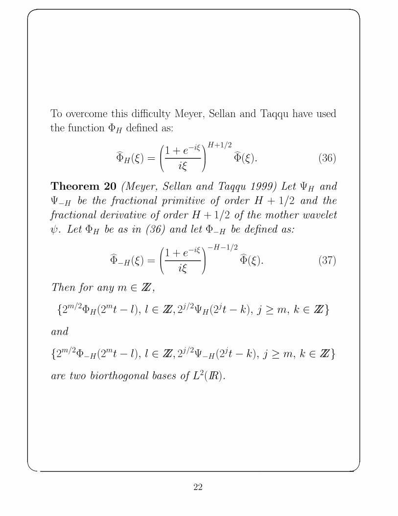
To overcome this difficulty Meyer, Sellan and Taqqu have used

the function ΦH defined as:

ΦH(ξ) =

1 + e−iξ

iξ

H+1/2Φ(ξ). (36)

Theorem 20 (Meyer, Sellan and Taqqu 1999) Let ΨH and

Ψ−H be the fractional primitive of order H + 1/2 and the

fractional derivative of order H + 1/2 of the mother wavelet

ψ. Let ΦH be as in (36) and let Φ−H be defined as:

Φ−H(ξ) =

1 + e−iξ

iξ

−H−1/2Φ(ξ). (37)

Then for any m ∈ ZZ,

{2m/2ΦH(2mt− l), l ∈ ZZ, 2j/2ΨH(2jt− k), j ≥ m, k ∈ ZZ}

and

{2m/2Φ−H(2mt− l), l ∈ ZZ, 2j/2Ψ−H(2jt− k), j ≥ m, k ∈ ZZ}

are two biorthogonal bases of L2(IR).

23

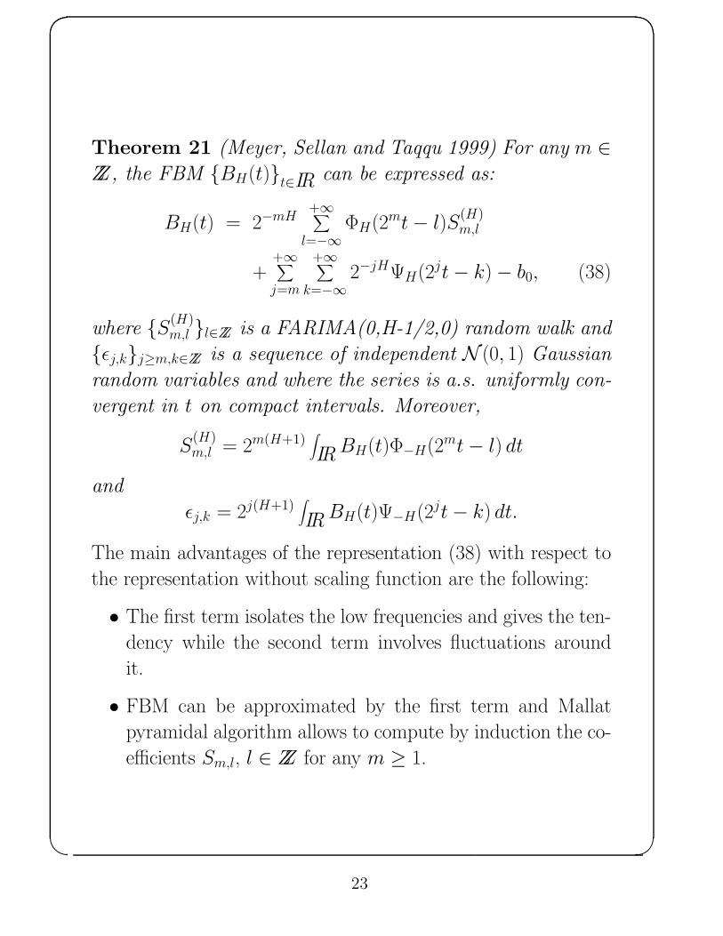
Theorem 21 (Meyer, Sellan and Taqqu 1999) For any m ∈ZZ, the FBM {BH(t)}t∈IR can be expressed as:

BH(t) = 2−mH+∞∑

l=−∞ΦH(2mt− l)S

(H)m,l

++∞∑

j=m

+∞∑

k=−∞2−jHΨH(2jt− k) − b0, (38)

where {S(H)m,l }l∈ZZ is a FARIMA(0,H-1/2,0) random walk and

{ǫj,k}j≥m,k∈ZZ is a sequence of independent N (0, 1) Gaussian

random variables and where the series is a.s. uniformly con-

vergent in t on compact intervals. Moreover,

S(H)m,l = 2m(H+1)

∫

IRBH(t)Φ−H(2mt− l) dt

and

ǫj,k = 2j(H+1)∫

IRBH(t)Ψ−H(2jt− k) dt.

The main advantages of the representation (38) with respect to

the representation without scaling function are the following:

• The first term isolates the low frequencies and gives the ten-

dency while the second term involves fluctuations around

it.

• FBM can be approximated by the first term and Mallat

pyramidal algorithm allows to compute by induction the co-

efficients Sm,l, l ∈ ZZ for any m ≥ 1.

24

4 Optimality of the wavelet representations of FBM

The representations without scaling functions are optimal in the

sense of Kuhn and Linde:

Theorem 22 (Taqqu and Ayache 2002) For every integer

J ≥ 0, let

FJ = {(j, k) ∈ ZZ2; 0 ≤ j ≤ J and |k| ≤ (J − j + 1)−22J+4},

and

PJ = {(j, k) ∈ ZZ2; −J ≤ j ≤ −1 and |k| ≤ 2J/2}.

For every integer n ≥ 2β with β = 64∑+∞l=1

1l2, let In ⊂ ZZ2 be

a set satisfying the following properties:

• In contains, at most, n indices (j, k),

• for every n ≥ 2β, FJ(n) ∪ PJ(n) ⊂ In, where J(n) is the

unique integer such that

(2β)2J(n) ≤ n < (2β)2J(n)+1.

At last let

BH,n(t) =∑

(j,k)∈In2−jH

(ΨH(2jt− k) − ΨH(−k)

)ǫj,k. (39)

Then there is a random variable C > 0 of finite moment of

any order such that a.s. for all n ≥ 1,

supt∈[0,1]

|BH(t) − BH,n(t)| ≤ Cn−H(1 + logn)1/2. (40)

25

The representations with scaling functions are optimal as well:

Theorem 23 (Taqqu and Ayache 2002) We suppose that

β, FJ and J(n) are the same as in Theorem 22. For every

integer J ≥ 0 let

QJ = {l ∈ ZZ; |l| ≤ 2J}. (41)

For every integer n ≥ 2β, let I ′n ⊂ ZZ and I ′′n ⊂ ZZ2 be two

sets satisfying the following properties:

• I ′n contains at most n/2 indices l and I ′′n contains at most

n/2 indices (j, k),

• for every n ≥ 2β, QJ(n) ⊂ I ′n and FJ(n) ⊂ I ′′n.

At last let

BH,n(t) =∑

l∈I ′nΦH(t− l)S

(H)0,l (42)

+∑

(j,k)∈I ′′n2−jH

(ΨH(2jt− k) − ΨH(−k)

)ǫj,k.

Then there is a random variable C > 0 of finite moment of

any order such that a.s. for all n ≥ 1,

supt∈[0,1]

|BH(t) − BH,n(t)| ≤ Cn−H(1 + logn)1/2. (43)

26

5 Concluding remarks

→ “The tensor products” of the wavelet series representations

of Fractional Brownian Motion lead to optimal series represen-

tations of Fractional Brownian Sheet.

→ Another optimal series representation of Fractional Brown-

ian Sheet has been introduced in 2003 by Dzhaparidze and Van

Zanten. It has some similarities with the expansion of Brownian

Motion in the trigonometric system.

→ Lifshits and Simon have recently used some wavelet tech-

niques for obtaining a sharp lower bound of the small ball prob-

ability of the symmetric α-stable Riemann Liouville process with

Hurst parameter H > 0, under a quite general norm.