Rate Handling Methods in Variable Amplitude Fatigue Cycle
114
Rate Handling Methods in Variable Amplitude Fatigue Cycle Processing By RYAN O’KELLEY A Thesis submitted in partial fulfillment of the requirements for the Honors in the Major Program in Mechanical Engineering in the College of Engineering and Computer Science and in the Burnett Honors College at the University of Central Florida Orlando, Florida Summer Term 2010 Thesis Chair: Dr. Ali P. Gordon, Ph.D.
Transcript of Rate Handling Methods in Variable Amplitude Fatigue Cycle

Rate Handling Methods in Variable Amplitude Fatigue Cycle Processing
By
RYAN O’KELLEY
A Thesis submitted in partial fulfillment of the requirements for the Honors in the Major Program in Mechanical Engineering
in the College of Engineering and Computer Science and in the Burnett Honors College at the University of Central Florida
Orlando, Florida
Summer Term 2010
Thesis Chair: Dr. Ali P. Gordon, Ph.D.

© 2010 Ryan O’Kelley

ABSTRACT
Predicting fatigue failure is a critical design element for many engineering
components and structures subject to complex service conditions. In high-temperature
and corrosive environments, many materials exhibit rate dependent phenomena that can
significantly alter safe service life predictions. Existing cycle processing techniques such
as Peak Counting, Simple Range, and the Rain Flow method are able to resolve complex
service histories into sets of simple cycles, but these methods are unable to handle time-
related parameters such as engage rate and cycle sequence. To address this, a cycle
processor was written in FORTRAN 95 later termed the Multi-Algorithm Cycle Counter
(MACC). This code was utilized as a platform to develop, test, and study various
methods of extracting and interpreting rate parameters extracted from cycles defined by
existing counting algorithms.

iv
ACKNOWLEDGMENTS
First and foremost I’d like to thank my thesis chair, Dr. Ali P. Gordon for
introducing me to the research field of engineering and pushing me to pursue excellence
in my academic and professional careers. His mentorship, enthusiasm, and
encouragement have opened opportunities in academia and industry that I otherwise
would not have been able to pursue. I’d also like to thank my thesis committee members
Dr. Seetha Raghavan and Dr. Ahmed Khalafallah for their involvement and support in
this research. Lastly, thanks to Scott Keller of the Mechanics of Materials Research
Group for his insight and advice on the procedures and expectations of academic research
at UCF.
A special thanks to my family and friends whose love, support, and gratitude kept
me going during difficult times and deflating setbacks.

v
TABLE OF CONTENTS
ABSTRACT ...................................................................................................................... iii
ACKNOWLEDGMENTS ................................................................................................ iv
TABLE OF CONTENTS ................................................................................................. v
FIGURE LISTING ........................................................................................................ viii
1. INTRODUCTION ....................................................................................................... 1
1.1 Background ......................................................................................................... 1
1.2 Objectives ........................................................................................................... 3
1.3 Overview .............................................................................................................. 4
2. BACKGROUND .......................................................................................................... 5
2.1 Single Parameter Algorithms ....................................................................... 6
2.2 Level Crossing ................................................................................................... 6
2.3 Peak Counting .................................................................................................... 8
2.4 Simple Range Method ................................................................................... 11
2.5 Double Parameter Methods ........................................................................ 12
2.6 Zero Parameter Methods ............................................................................. 15
2.7 Rate-Dependence ........................................................................................... 16
3. Research Approach .............................................................................................. 17
3.1 Preliminary Procedures ................................................................................ 17
3.2 Resolving Reversal Points ........................................................................... 19
3.3 Peak Counting .................................................................................................. 20
3.4 Simple Range ................................................................................................... 22

vi
3.5 Rain Flow ........................................................................................................... 23
3.6 RMS ...................................................................................................................... 23
3.7 Rate Handling .................................................................................................. 24
3.8 Post Processing and the Fast Fourier Transform Method ............... 26
3.9 User Interface .................................................................................................. 27
4. RESULTS ................................................................................................................... 30
4.1 Algorithm Validation ...................................................................................... 30
4.2 Algorithm Performance ................................................................................ 32
4.3 The Simple Signal .......................................................................................... 32
4.4 The 2Ssum Signal .......................................................................................... 35
4.5 The 3sum cycle ............................................................................................... 39
4.6 Random Cycling .............................................................................................. 42
4.7 Rate Handling .................................................................................................. 46
4.8 Simple Signals ................................................................................................. 47
4.9 Noisy Continuous Signals ............................................................................ 47
4.10 Relative Performance ................................................................................. 49
4.11 Discontinuous Load Signals ..................................................................... 51
4.12 Relative Performance ................................................................................. 52
4.13 Computational Performance .................................................................... 53
5. Applications ............................................................................................................. 56
5.1 Offshore Structures ....................................................................................... 56
5.2 Land-based Structures ................................................................................. 59
5.3 Automotive Components ............................................................................. 63
6. CONCLUSIONS AND FUTURE WORK ............................................................. 69

vii
6.1 Cycle Counting ................................................................................................ 69
6.2 Rate Handling .................................................................................................. 71
6.3 Future Research .............................................................................................. 72
APPENDIX A: SOURCE CODES ............................................................................. 74
APPENDIX A.1: MACC PARENT MODULE (main.f90) ................................ 75
APPENDIX A.2: MACC GLOBAL NAMESPACE MODULE (global.f90) ... 77
APPENDIX A.3: MACC SUBROUTINE MODULE (subs.f90) ...................... 78
APPENDIX A.4: MATLAB POST PROCESSING .............................................. 96
APPENDIX A.5: C# MACC GUI .......................................................................... 98
APPENDIX A.6: MATLAB RATE ANALYSIS ................................................... 100
APPENDIX A.7: MACC Parameter File (params.txt) ............................... 102
REFERENCES .............................................................................................................. 103

viii
FIGURE LISTING
Figure 1.1. Strain-rate dependence of fatigue life of AISI 304L at 973 K [5] .................... 2
Figure 1.2. S-N Curve used in traditional variable amplitude fatigue analysis [1] ............ 3
Figure 2.1. Basic fatigue loading parameters [7] ................................................................ 6
Figure 2.2. (a) Sample service history data and (b) resolution by the Level Crossing
method [7]. .......................................................................................................................... 7
Figure 2.3. (a) A sample service history, (b) simple cycles resolved by the Mean Crossing
Peak Counting method and (c) simple cycles resolved by Peak Counting [8]. ................ 10
Figure 2.4. Service history resolution by the Simple Range method [8] .......................... 12
Figure 2.5. Application of the Rain Flow method ............................................................ 14
Figure 3.1. Typical service history text file ...................................................................... 18
Figure 3.2. Reversal point being incorrectly resolved by central finite differencing ....... 19
Figure 3.3. MACC system flowchart ................................................................................ 27
Figure 3.4. MACC GUI form ........................................................................................... 28
Figure 4.1. Code snippet from the MACC service history emulator library .................... 31
Figure 4.2. Simple and complex service histories ............................................................ 31
Figure 4.3. Simple sine/cosine service history .................................................................. 33
Figure 4.4. Simple service history resolved into reversal points ....................................... 33
Figure 4.5. Peak Counting method applied to the simple service history ......................... 34
Figure 4.6. Simple Range method applied to the simple service history .......................... 34
Figure 4.7. Rain Flow method applied to the simple service history ................................ 35
Figure 4.8. 2Sum service history ....................................................................................... 36
Figure 4.9. 2sum service history resolved into reversal points ......................................... 37

ix
Figure 4.10. Peak Counting method applied to the 2sum service history ......................... 37
Figure 4.11. Simple Range method applied to the 2sum service history .......................... 38
Figure 4.12. Rain Flow method applied to the 2sum service history ................................ 38
Figure 4.13. 3sum service history ..................................................................................... 40
Figure 4.14. 3sum service history resolved into reversal points ....................................... 40
Figure 4.15. Peak Counting method applied to the 3sum service history ......................... 41
Figure 4.16. Simple Range method applied to the 3sum service history .......................... 41
Figure 4.17. Rain Flow method applied to the 3sum service history ................................ 42
Figure 4.18. Random service history ................................................................................ 44
Figure 4.19. Peak Counting method applied to the random service history ..................... 44
Figure 4.20. Simple Range method applied to the random service history ...................... 45
Figure 4.21. Rain Flow method applied to random service history .................................. 45
Figure 4.22. Extraction method diagram .......................................................................... 46
Figure 4.23. Rate examination of a simple signal ............................................................. 47
Figure 4.24. Rate examination of the 2sum half-cycle ..................................................... 48
Figure 4.25. Rate examination of the 3sum half-cycle ..................................................... 49
Figure 4.26. Relative extraction performance with increasing signal complexity (Simple
signal reference) ................................................................................................................ 50
Figure 4.27. Relative extraction performance (RRE method reference) .......................... 50
Figure 4.28. Rate examination of a step cycle .................................................................. 51
Figure 4.29. Rate examination of the step2sum half-cycle ............................................... 52
Figure 4.30. Relative extraction performance on discontinuous signals (step reference) 53

x
Figure 4.31. Relative extraction performance on discontinuous signals (RRE Reference)
........................................................................................................................................... 53
Figure 4.32. CPU time used in MACC execution - Step input ......................................... 54
Figure 4.33. CPU time used by Rain Flow method - 2sum signal .................................... 55
Figure 5.1. Offshore structure service history sample ...................................................... 57
Figure 5.2. RRE method applied the offshore service history .......................................... 58
Figure 5.3. CFDA method applied to the offshore service history ................................... 58
Figure 5.4. Linear LSR method applied to the offshore service history ........................... 59
Figure 5.5. Extraction method comparison (offshore structure) ....................................... 59
Figure 5.6. Land-base structure service history sample .................................................... 61
Figure 5.7. Secondary cycles from the Land-base structure service history .................... 61
Figure 5.8. RRE extraction method applied to the land-based structure service history .. 62
Figure 5.9. CFDA extraction method applied to the land-based structure service history 62
Figure 5.10. Linear LSR extraction method applied to the land-based structure service
history ............................................................................................................................... 63
Figure 5.11. Extraction method comparison (land-based structure) ................................. 63
Figure 5.12. Automotive axle service history ................................................................... 65
Figure 5.13. Single cycle from the automotive axle service history ................................. 65
Figure 5.14. RRE extraction method applied to the automotive axle service history ...... 66
Figure 5.15. CFDA extraction method applied to the automotive axle service history .... 66
Figure 5.16. LSR extraction method applied to the automotive axle service history ....... 67
Figure 5.17. Comparison of engaging rates (automotive) ................................................ 67
Figure 5.18. Comparison of disengaging rates (automotive) ............................................ 68

1
1. INTRODUCTION
1.1 Background
It could be argued that fatigue failures are inevitable in mechanical systems. If a
component subject to cyclic loading does not fail due to overload, shock, corrosion, wear,
or other modes of failure, it will eventually succumb to fatigue. Generally, designs of
components are over-engineered to ensure that the life cycle of the product outlasts any
warranty or legal liability. These oversights very often increase production and life-cycle
costs, while decreasing product performance. One goal of further fatigue research is to
develop methods that lead to maximum utilization of mechanical products.
A component or structure subject to cyclic loading either has or has not failed by
some arbitrary definition (i.e., visible crack formation). The nature of the failure criterion
is generally discreet, but the time-dependent relationship suggests that the phenomenon is
actually continuous with time; a mechanical component appears to be able to withstand a
certain number of loading events before sudden failure. This sets the stage for various
constructs to bridge the gap between the failed and functional states—the ultimate goal of
these constructs being to rate the remaining functional service life of the component.
The facet of interest in this research is the improvement of fatigue failure prediction
through more thorough service history analysis. More specifically, this research
concentrates primarily on improving the existing cycle counting methods used to analyze
service history data. Pivotal concepts and assumptions used in such approaches are:
Elements subject to variable amplitude service have a finite service life [1]
Service life can be estimated by (1) condensing the service history data into cycle events (cycle counting) [2], (2) estimating damage incurred be each cycle event [3], and (3) accumulating the damage incurred by each event [1].

2
Continuing developments in the power generation industry have lead to larger, higher
temperature and higher pressure gas and steam turbines that require more robust
components than ever [4]. Because the material prices of austenitic stainless and Ni-base
superalloys continues to rise, many manufacturers aim to optimize component designs to
reduce initial manufacturing costs, and reduce life-cycle costs by increasing time
intervals between inspection outages. One such opportunity for optimization is increasing
the service life of a component by accounting for rate-dependence in fatigue life
estimation. Figure 1.1 shows a typical example of fatigue life dependence on strain rate.
Here the material exhibits two distinct regions of strong and weak strain-rate dependence.
If rate data is not included in analysis, there are two possible consequences: (1) assuming
fatigue resistance from the weak region will lead to overly conservative life estimates
when high rate events are superimposed with low rate events or (2) assuming fatigue
resistance from the strong region will result in non-conservative estimations of fatigue
life.
Figure 1.1. Strain-rate dependence of fatigue life of AISI 304L at 973 K [5]

3
In the typical setting, single-variable S-N data is used to develop a relationship
between fatigue strength and number of repetitions to failure shown in Figure 1.2. In this
data, material composition, condition, temperature, pressure, and cycle rate are assumed
constant. Specific to this application, each load event magnitude is cast as a fatigue-
strength, and the relationship is used to determine Nf, the number of repetitions to failure.
Figure 1.2. S-N Curve used in traditional variable amplitude fatigue analysis [1]
Knowing this, and the number of repetitions that occurred during a service history,
Miner’s linear damage accumulation rule is used to establish the percentage of functional
life consumed by the load event [3,4,6]. This procedure is repeated until all loading
events are resolved and accounted for. Although the analysis of damage accumulation
theory is outside the scope of this research, it is the primary motivating factor behind the
incorporation of rate parameters.
1.2 Objectives
Rather than utilizing a single parameter relationship to determine Nf, the number
of repetitions to failure, this research aims to explore complementing this quantity with a

4
rate dependent metric derived from the complex service history. Capturing rate along
with cycle magnitude can more accurately model the accumulation of damage throughout
a complex service history. The main obstacle in utilizing such a technique is the lack of
support for extracting cycle rate parameters in existing counting procedures [7]. The
primary objective of this research is to develop and characterize methods for extracting
rate parameters from post-processed service histories. In order to make any substantial
observations about the validity of the rate extraction methods to be developed, the
fundamental operation of the employed counting algorithms needed to be understood to
develop a consistent and meaningful definition of a cycle. To exhibit and address the
issue of cycle rate extraction in existing cycle processing algorithms, existing cycle
counting procedures were developed, tested, and modified.
1.3 Overview
Once the algorithms of interest had been developed into programmable procedures,
they were integrated into the Multi Algorithm Cycle Counter (MACC) code and
subjected to a range of simple and idealized service histories. Performance characteristics
such as processing time, number of cycles identified, feature expandability, and cycle
validity were documented to serve as a comparison metrics to rank methods included in
the MAAC program. The next chapter of this thesis details pertinent prior research on
fatigue cycle counting. Afterwards, the analytical approach of this research is discussed
and in Chapter 4 the test results of standard and modified counting algorithms are
covered. Chapter 5 applies these results in industry-specific case studies to examine the
aggregate performance of the rate extraction methods.

5
2. BACKGROUND
Cycle counting in this context is the resolution of a complex service history that is
either too long or too complicated to count visually into a series of simple cycles that can
be processed by a damage accumulation rule. The ASTM standard E 1049 [7] provides
an adequate definition of some commonly used algorithms, but it does not mention a
procedure for selecting an algorithm or the environment-dependence of their
performance. Other fatigue texts also only outline the basic procedures of the various
counting algorithms [3,6,8]. Industry publications such as the ASM International
Handbook on Fatigue and Fracture [9] only mention the use of an “adequate” cycle
counting method and do not formally define criteria for such a counting method. The
above mentioned literature also provides little insight into developing these concepts into
numerical procedures for practical use; analysis of this literature reveals a considerable
gap between the formal definition of these methods and programming solutions required
for their implementation. The prospect of rate and sequence extraction also goes virtually
unmentioned. The literature referenced in this work served mainly to define the
framework of the cycle counting methods as there has apparently been very little or no
known research resulting in publications relevant to the main scope of this project. An
exhaustive literature review has resulted in no widely available works addressing rate
extraction. The counting algorithms are commonly grouped by the number of potential
cycle parameters taken into consideration when the cycle is being defined. The single,
double, and zero-parameter methods are described in the following sections.
6
2.1 Single Parameter Algorithms
The single parameter approaches are more often used in demonstration than in
industrial application [6,7,10]. This algorithm group analyzes a single parameter (i.e.,
difference between points, point value, etc.) to reconstruct a simple cycle and typically
cannot properly resolve noise, secondary signals, or other highly complex signals.
Figure 2.1. Basic fatigue loading parameters [7]
2.2 Level Crossing
When single parameter methods are defined, level-crossing counting almost
universally appears first. The Level Crossing procedure starts with the definition of a
reference load level. The load space (or axis) must then be divided into a meaningful
number of subdivisions. Two categories of counts are defined: when the load data crosses
a division line with a positive slope, a Category I count is made. When the load data
crosses a division line with a negative slope, a Category II count is made. Once all
sections of the load data are resolved, the elements are reassembled to form the most
damaging cycles. Starting at the reference load level, sequentially larger Category I
counts are assembled until there are no larger values. Starting at the last level,
sequentially smaller Category II counts are assembled until the reference load level is
7
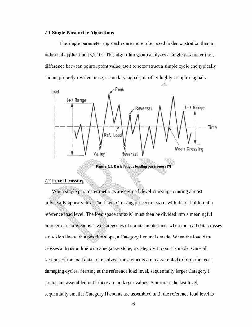
reached. This procedure is repeated in the negative load direction until all sections are
accounted for. Figure 2.2 shows a typical service history before and after the application
of the Level Crossing method. In this figure, the reference load level is assumed to be
zero which imposes the requirement that each cycle stem from and return to this level.
Reconstruction of the service data reveals the high magnitude master cycle, but combines
several of the slave cycles into a more damaging, high amplitude cycle. Only two noise
cycles are identified; several are lost in the load space subdivisions and others are
consumed by higher magnitude cycles.
Figure 2.2. (a) Sample service history data and (b) resolution by the Level Crossing method [7].
Visually, and without any consideration of error tolerances, the Level Crossing
technique is relatively simple but extremely tedious to execute. The method dissects the
service history into differential elements and reconstructs simple cycles using these
elements. In practice, this method yields some impressive obstacles. A reoccurring theme

8
among this and other single-parameter methods is the definition of a reference load level.
Among relatively simple service histories this may be observed visually (i.e., overall
average load), but this idea in principal contradicts the motivation behind utilizing such
an algorithm: to resolve complex service histories (i.e., situations where the history
cannot be resolved visually). In common with many other single-parameter methods is
the complete rearrangement of load values, invalidating any rate or sequence information.
Further, dividing the load space into a “meaningful” number of sections is not formally
defined in literature. For a given service history, the number of divisions could be
increased until the cycle count does not exhibit any significant change; however, this also
contradicts the underlying goal of these algorithms as the count would be performed
indefinitely until an optimal environment is created. Further still, the method does not
actually define any procedure for the counting of cycles. Only cycle reconstruction is
outlined in this method. An additional procedure such as Peak Counting or Simple Range
must be used on long service histories where the reconstructed cycles cannot simply be
counted visually.
2.3 Peak Counting
One of the more intuitive single-parameter methods is Peak Counting. In common
with the majority of the algorithms, the Peak Counting method cannot operate directly on
service data. The service data must first be resolved into reversal points (i.e., local
maxima and minima) [7,8,10]. There are several variations of the Peak Counting method
found in literature. The most commonly used variation evaluates only local maxima
above the reverence level and local minima below the reference level. These points are
later paired to form cycles (Figure 2.3 (b)) [7]. This variation can lead to highly non-

9
conservative damage estimation as a large portion of reversal points can potentially be
discarded. This method imposes the assumption that all cycles must cross through the
reference level. Another variation simply pairs the largest available sets of maxima and
minima to form cycles (Figure 2.3 (c)) [7]. This variation tends to yield more
conservative damage estimations in that many secondary or noise cycles can be counted
as reference level-crossing, high magnitude cycles. Because this research aims to use this
method as an upper bound for counting solutions, the latter is further explained in detail.
The procedure starts with the definition of a somewhat arbitrary reference load level.
Often times, the overall history average is used. Similar to many cycle counters, the load
data must be resolved into reversal points. The largest and smallest reversal values are
then paired until all points have been accounted for in a cycle. The difference between
each pair is recorded as the cycle range and the mean can be recorded as the average of
the pair. The cycle mean will by nature be biased toward the reference level and
therefore, is generally disregarded. A demonstration of the Peak Counting method is
shown in Figure 2.3. In this figure, because the service history is identical to that of
Figure 2.2 (a), the reference strain level is assumed to be zero. Figure 2.3 (b) shows the
Peak Counting method correctly resolving the high amplitude master cycle. Like the
Level Crossing method, the Peak Counting method implicitly combines portions of noise
cycles to form a medium amplitude cycle (cycle F-G) but yields a significantly more
conservative counting solution as noise is cast as higher magnitude cycles.

10
Figure 2.3. (a) A sample service history, (b) simple cycles resolved by the Mean Crossing Peak Counting method
and (c) simple cycles resolved by Peak Counting [8].
As with the Level Crossing technique, there is no formally defined method to
determine a meaningful reference load level when using the Peak Counting method. In
principal, the Peak Counting method assumes that the service history begins at the

11
reference load level, moves to a high peak value, back to the reference load level, moves
down to a low peak value, and back to the reference level once again to form a complete
reversal using only the peak and valley points as evidence. These assumptions propagate
each cycle average to the overall history average, and therefore mean stress or strain
effects cannot be accounted for. In common with the Level Crossing technique, this
method also requires the complete rearrangement of load data, invalidating all rate and
sequence information.
2.4 Simple Range Method
The Simple Range method is one of the more sophisticated single-parameter cycle
counting algorithms. Similar to the Peak Counting method, the Simple Range algorithm
cannot operate directly on service history data so it must first be resolved into a set of
reversal points. Where the Level Crossing method divides the history into differential
units, and the Peak Counting method examines peaks, the Simple Range method
examines ranges, or differences between sequential reversal points. The difference
between sequential points is calculated and each value is counted as a half cycle. Figure
2.4 demonstrates this method on a complex service history. In this figure, the simple
range method fails to correctly resolve noise and secondary cycles to uncover the master
cycle (range D-G). The master cycle is misrepresented and masked by noise at a range of
six units. Visual inspection reveals the master cycle at a range of nine units.

12
Figure 2.4. Service history resolution by the Simple Range method [8]
At the fundamental level, there are no major application issues stemming from the
Simple Range method. An arbitrary reference level is not required, few operational
assumptions are made, rate and sequence information are preserved, and partial cycles are
handled in an effective manner. However, signals with a large amount of noise will
completely mask underlying high-amplitude cycles as each reversal pair is discarded after
being resolved as a half-cycle.
2.5 Double Parameter Methods
The double parameter methods generally yield the most accurate and reliable
cycle counts [10]. In this group of counting algorithms, pairs of cycle parameters are

13
analyzed for cycle candidacy which allows for the proper resolution of noise and
secondary cycles. The algorithm that best characterizes the double parameter methods is
the Rainflow method developed by Endo and Matsuiski [11]. Although this method is not
possible to implement numerically the way Endo and Matsuiski describe it, there are
multiple numerically compatible adaptations available [3,6,8]. This algorithm adequately
resolves noise, identifies hysteresis behavior [10], and is capable of retaining time data
for cycles.
The ASTM standard E 1049 [7] contains a definition of the Rain Flow method
that is much simpler than the Rain Flow analogy used in many texts [6,8,10] . Similar to
previously mentioned methods, this procedures starts with the resolution of the load data
into reversal points. The first, second, and third reversals are cast as points i, j, and k,
respectively. The procedure continues by evaluating the difference (or range) between
points i and j, and points j and k. If the j-k range is larger than that of the i-j range, the i-j
range is counted as a full cycle and the point j is discarded from further analysis. The
procedure continues by recasting the i-j-k indices onto remaining reversal points and
repeats this procedure until only two reversal points remain. The range of this remaining
pair is counted as a half-cycle. There are also some exceptions to this procedure. If point i
is the beginning entry in the reversal data and a cycle is discovered, point i is discarded
rather than point j. Figure 2.5 is a visual representation of the ASTM Rain Flow
procedure with the starting point exception in use. Starting at Point B, the A-B range is
counted as a reversal because the B-C range is larger. Because Point A is a starting point,
it is discarded rather than Point B. Upon visual inspection, this method appears to
correctly unmask the high amplitude master cycles without altering the lower magnitude

14
secondary cycles. Because the reversal data is not rearranged or altered in the process, the
counted cycles also retain their mean, sequence, and rate parameters.
Figure 2.5. Application of the Rain Flow method
The vast majority of the double parameter methods yield closely grouped results
when applied to the same service history. Hayes Method, Range Pair, Ordered Overall
Pair, Racetrack, and the Hysteresis Loop method all yield virtually identical cycle counts
as the Rainflow method when load data is arranged in the same manner [7]. The double

15
parameter methods are all driven by the same objective: the identification of hysteresis
loops and the extraction of their parameters.
2.6 Zero Parameter Methods
The zero parameter cycle counting algorithms are best employed in scenarios
where more in-depth analysis would not be meaningful or economical. Long, random and
invariant loading histories where the primary objective is to study the effects of noise and
vibration on fatigue life are typical candidates for the Zero Parameter methods. Two
commonly used algorithms are the RMS Method and the Fourier Transform Method.
Applications primarily subject to vibration or high-speed, random loading where
the amplitude of oscillation is significantly larger than any discontinuous events in the
service history may be represented via the Root Mean Square (RMS) method. The proper
use of the RMS method is neither widely published nor standardized, but most of its
applications construct an equivalent, constant amplitude master cycle based on the RMS
value of the high and low reversal points. The number of reversal points is assumed to be
directly proportional to the number of cycles [3,12]. Once the RMS equivalent range is
computed, pairs of reversal points are counted as complete cycles. This method removes
all time related information from the load data and refines it to only two parameters:
RMS equivalent range and the number of cycles.
Applications that are subject to a sum of time-continuous, sinusoidal load signals
based on an analytic function can benefit from the use of a Fourier transform [13,14,15].
By transforming the load signal from the time domain to the frequency domain, the
amplitude and frequency of major sinusoidal load events can be extracted by identifying

16
the peak points in the transformed function. Knowing the frequency of a signal allows for
an interpolation of the number of repetitions that occur in a fixed time frame.
Relative to other commonly used methods, Fourier analysis has the narrowest of
applications. Any non-periodic events will be neglected, and any non-sinusoidal signals
will be erroneously represented as low-amplitude noise due to the nature of the Fourier
Transform.
2.7 Rate-Dependence
Rate dependence of materials is well known and documented facet of materials
testing [5,16,17,18]. Monotonic room temperature experiments on high-performance
steels show increases in yield strength on the order of 10% and more [19]. Materials
subject to high-rate conditions appear to react to loading events with higher strength as
potential dislocations within the material do not have adequate time to reach a steady
state and permeate [18]. Further research shows that the overall effect of an increased
cycle rate on fatigued components in high-temperature environments can dramatically
increase fatigue life. More importantly, the effect of low cycle rates is significantly
decreased fatigue life [5] which may lead to premature failure. This study aims to
develop a framework in which these effects can be accounted for by analyzing various
cycle definitions used in literature and using these algorithms as a platform for
developing rate handling procedures for further testing.

17
3. Research Approach
In order to analyze cycle data, programmable algorithms are required. Existing
software such as AFGROW, RAINFLOW from Durability, Inc. and STOFLO contain
adequate cycle counters, but generally no commercially or publically available source
codes are available to utilize as a platform for further research and development of the
cycle counting methods. A small software package outlined in Figure 3.3 was written as a
part of the current study to investigate rate handling procedures. The Multi-Algorithm
Cycle Counter (MACC) given in Appendix A.1-A.3 accurately implements the cycle
counting algorithms outlined in the ASTM E 1049 standard and allows for augmentations
such as the addition of rate extraction procedures.
The remaining sections of this chapter detail with structure and operation of the
MACC code and conclude with a discussion of the research approach. In the final section
it will be clearly stated how the hypothesis will be proven or disproven.
3.1 Preliminary Procedures
As is the case with most cycle counters, the MACC program is coded under the
assumption that the service history data has already been collected and is assembled in
either a comma separated, space separated, or tab separated values in an ASCII text file
where column zero contains the time stamp, and column one contains the service data,
either stress, strain, force, torque, etc.

18
Figure 3.1. Typical service history text file
Only one channel of service history is used in the current study. For the case of multi-axis
loading, multi-channel analysis would need to be implemented into the MACC code and
is saved for future study. Using the FORTRAN inquire command, the service history text
file is probed to ensure any exceptions are handled and the user is returned a meaningful
error message in case the file was not found, or unavailable. Once the availability of the
file is ensured, it is opened and checked by stepping through each line and counting the
number of entries. If no entries are found, the exception is handled by returning an error
message and terminating the program. If the file has at least one entry, a dynamic array is
allocated to match the dimensions of the text file and its contents are loaded into memory.
Due to the potentially large number of entries to be loaded for long service histories, the
heap memory segment is utilized rather than the default stack segment resulting in a
slight decrease in performance but great increase in reliability when handling large
arrays. In addition, program parameter and material property texts files are loaded into
arrays to complete the initialization of the program.

19
3.2 Resolving Reversal Points
Because the vast majority of the counting algorithms cannot operate directly on
service data, the first major operation in the MACC code is the resolution of reversal
points. Resolving the service history into reversal points was accomplished using a
relatively primitive technique. Preliminary attempts required the use of central finite
differencing. Using a series of loops and conditional statements, points central to a
minimum derivative were identified as local maxima and minima. However, when
relatively low resolution load data was fed into the program this procedure routinely
misidentified peak points with an error of ±1 indexed entry. Figure 3.2 illustrates such an
example: the numerical first derivative minimum occurs at index number two, but the
reversal point clearly occurs at index number one.
Figure 3.2. Reversal point being incorrectly resolved by central finite differencing
In light of this situation, a more primitive approach was taken to resolve the reversal
points. The routine in the MACC program steps though the history array and observes the
surrounding two nearest indexed values to see if they are either both greater than or less
than the value at the index in question. If both surrounding values are greater than the
‐2
‐1.5
‐1
‐0.5
0
0.5
1
1.5
2
2.5
3
3.5
0 1 2 3 4 5
Value (unit)
Time (unit)
Value
First Derivative

20
value in question, the point is defined as a local minimum. The same logic applies for
local maxima. Because the number of reversal points cannot be determined in advance,
pre-allocating the storage array for this information is not possible. Therefore, this routine
requires two passes to complete. The first pass simply counts the number of reversal
points and allocates resources for a properly sized array. The second pass re-identifies the
reversal points and dumps the time stamp and value of each point to a local
maxima/minima array declared local. A more efficient protocol that could be used in
place of this method is array flagging. The initial service history array could have been
allocated with an additional empty column. The reversal point locating routine simply
could have flagged reversal points by adding a flag value to the array at the index
location of a reversal. However, this method would have significantly complicated
referencing reversal points from other subroutines.
3.3 Peak Counting
Of the cycle counting methods focused on in this thesis, Peak Counting
(Appendix A.3) is the most computationally expensive. To initialize the procedure, a
reference load level must be defined. Because there are no published guidelines for
defining the reference level, the MACC program is coded to take the overall average of
the reversal values. Once the reference level is defined, the routine aims to sort the
reversal points into two bins: points above the reference load level, and those below. A
reoccurring theme in the development of this chapter is memory management. Because
the size of the bin arrays is not known a priori, this procedure also requires two passes to
execute; each is described.

21
The first pass steps through the local array to count the number of points above
the reference level, and those below. Once complete, the second pass dumps the values
into the max and min arrays without their respective timestamps. The next step in the
procedure is by far the most computationally expensive routine in the MACC program.
To reiterate, the goal of this method is to combine the reversal points in such a way that
each cycle incurs the maximum possible damage without reusing any points. In order to
achieve this, a sorting algorithm was employed to arrange the high and low bins in a way
such that their values could be paired sequentially by stepping through each array and
simply extracting and pairing the next value. For the scope and application of this
program, a simple bubble sort routine was employed to sort the bins from their highest to
lowest values. The routine looks at the first value of an array for an initial value and steps
though the array to find the largest value using a series of conditional statements and
circular references. Once the largest value is found, the value is copied to the first
available index in a new array, and the procedure is repeated until all values are resolved.
A similar procedure is performed on the low-value bin array.
Once the new sorted bins are filled, values from each bin at the sequential row
indices are paired to form cycles. For example, the largest value from the high-bin is
paired with the lowest value from the low-bin to from a cycle. These points are discarded
and the next set of points are paired to form a cycle. This procedure continues until all
points are resolved. If the high-bin and low-bin arrays are not equal length, the trailing
value is paired with the reference level to form a half cycle. The only cycle parameter
that can be extracted using this method is amplitude. Because the procedure assumes that

22
the load signal stems and returns to the reference level, nearly every cycle average will be
either at or very close to the reference level.
The bubble sort routine may be one of the least efficient implementations of a
sorting algorithm known to computer science [20] but has been integrated into the Peak
Counting subroutine shown in Appendix A.3. If the MACC program were to be prepared
for application in industry, this routine would undoubtedly need to be replaced by either
the Quicksort or Heapsort routines [21], depending on the length of the service history in
question, to achieve more reasonable computational efficiency.
3.4 Simple Range
As the name implies, the Simple Range method reduces to a relatively simple
programming procedure. The routine steps though the local reversal array, observes the
first and second values, computes their difference and dumps this value into a new array.
This procedure is repeated until all reversal points are resolved and each value in the new
difference array is counted as a half cycle. Additionally, the average of each reversal pair
can be cast as the cycle mean. The average half-cycle rate is also extracted by dividing
the cycle amplitude by the difference in time stamps between the parent reversal points.
Memory management is also exceptionally simple in this method; the size of the
difference array can be determined by dividing the size of the local reversal array by two.
If the reversal array contains an odd number of entries, the trailing value must be
discarded as there is no meaningful procedure to handle what is effectively a quarter-
cycle. The text version of this algorithm is shown in Appendix A.3.

23
3.5 Rain Flow
The Rain Flow analogy could be one of the least straightforward methods to
convey the method, and unfortunately is used almost universally to explain the concept
behind this procedure. A more concise definition is found in the ASTM E 1049 standard
for cycle counting standard practices, and such was utilized in the development of the
MACC application. The fundamental operation of the Rain Flow routine is simple: the
second index in the reversal array is used as a starting point. Next, the difference between
this point, the next index value and the previous index value are computed. A series of
conditional statements evaluates if the next range greater than the last. If this statement
returns true, a full cycle is counted whose amplitude matches that of the previous range,
and the current central point is discarded. The procedure was implemented by means of
array flagging. First, the reversal array is copied to a new working array with an
additional blank column. When a cycle is identified in this new working array, a flag is
added into the blank column at the index of the central value effectively discarding the
value. The cycle amplitude, mean, timestamps, and original array indexes are dumped to
a new array for later analysis. Because the working array has now effectively been
modified, the routine must restart from the first available index and start over, avoiding
flagged indexes—characteristic of the Rain Flow algorithm. The FORTRAN routine is
provided in Appendix A.3.
3.6 RMS
There are two instances of the RMS method in the MACC program. The first is
based on the technique outlined in the ASTM STP 748 publication on the subject [22],
and the second uses the RMS calculation in its typical sense for comparison. The ASTM

24
method requires that the load reversal array be sorted into max and min bins before
operation. The sorting criteria for these bins are largely undefined. Based on examples
from the publication, and in other deployments [12] the routine used in the MACC code
was designed to sort based on a reference level similar to the Peak Counting routine.
Once the load reversal array was sorted into high and low bins, the RMS of each was
calculated. The difference in the RMS value from each bin is cast as the master cycle
range, and the number of counts is defined as half of the number of reversal points.
Because the RMS value is always positive, the code transfers the signs of the means of
the reversal points to the RMS values before computing their difference.
The second instance of the RMS method utilizes the RMS calculation in its
typical sense. This routine calculates the overall RMS magnitude of the service history.
The RMS value is cast as the master cycle magnitude, and the number of counts is
defined similarly to the ASTM method. Both methods are included in the MACC source
code given in Appendix A.3.
3.7 Rate Handling
Methods in the MACC program that supported the meaningful extraction of
average rate information were modified to do so. In the single parameter methods, this
was accomplished by simply dividing each cycle amplitude by the difference in time
stamps from the parent reversal points (change in value per change in time). Because the
Rain Flow method is a double parameter method constructed of three points (and
therefore, two segments) separate increasing and decreasing rates were extracted for each
cycle. In all cases, rate information was augmented to the cycle count array for each
method. This technique operates at the reversal level and was termed RRE, for reversal

25
rate extraction. Issues mentioned later in this paper prompted the need for additional rate
extraction techniques, the first of which was a load-level average rate extraction (as
opposed to peak-level rate extraction). Rather than operating on the reversal points to
obtain rate parameters for a cycle, this method averages the first time-derivative of the
service history data within each cycle window and records this value as the average cycle
rate. This was implemented in the MACC program by augmenting the service history
array with a central finite difference time derivative of the load values and was termed
the Central Finite Difference Average (CFDA) method. Each applicable cycle counting
routine was modified to call such a routine during operation. During counting operations
the original array indices from the service history data were used to map a window to the
load rate data. Once this window was defined, the statistical mean and standard deviation
were computed and recorded for later analysis and the counting routine continued.
Similar to earlier mentioned methods, the single parameter procedures yield a single rate
per cycle, and the double yield two rates per cycle (load and unload). The rate handling
subroutine was developed to run in several different modes triggered by the parameter
file (params.txt) during startup. The routine operates in either RRE, CFDA, Linear LSR
mode.
Linear LSR (least squares regression) mode extracts the rate data from a more
advanced statistical approach. Using the same load window defined above, the series of
points are fitted with a linear least squares regression line and the slope is recorded as the
cycle rate (or cycle engage and disengage rates for double parameter methods). The
mathematical definitions are given in Equations 1-3. In these equations, the symbol α
(alpha) represents the service history value (stress, strain, load, deflection, etc.) and n

26
represents the cycle window indices. Text versions are given in the MACC source code
(Appendix A.1-A.3).
(1)
∑
(2)
∑ ∗ ∑ ∗
∑ ∑ ∗ ̅
(3)
3.8 Post Processing and the Fast Fourier Transform Method
Due to the complexity and narrow application of the Fast Fourier Transform
(FFT) method, this method was not included into the MACC code. Instead, this method
was employed in the post processing phase of analysis through MATLAB. Once the
MACC program had been successfully executed on a service history, the input and output
data files were passed to MATLAB for further analysis and plotting. Once these data files
are loaded into the MATLAB environment, the built-in FFT function (Cooley-Tuckey
algorithm [23]) is used to analyze the service history [24]. The result of this is a plot of
the transformed load data from the time domain to the frequency domain. The remainder
of post processing operations are the sorting of the cycle parameter packages (amplitude,
mean, and rate) into bivariate histograms with cycle amplitude and cycle mean as the
variations. These diagrams were used to exhibit the relative performance of each

27
counting method included in the MACC program. The MATLAB post processing code is
given in Appendix A.4.
Figure 3.3. MACC system flowchart
3.9 User Interface
To simplify operation, a GUI was written in Microsoft’s Visual C# language.
Without this element, experimentation could only be performed through the manipulation
of the MACC source code. Because C# is a relatively powerful language compared with
FORTRAN, for development was handled largely by Microsoft’s .NET code framework.
The form allows the selection of a service history text file, the selection of an output
folder, and variation of various MACC runtime parameters such as counter selections,
units, etc. The program uses the user defined switches and values to write a MACC
runtime parameter file (Appendix A.7) used to define various processing options.

28
Figure 3.4. MACC GUI form
To interact with the parameter file, many of the MACC program variables were
passed to the global namespace module; this greatly simplified the movement of
information throughout the system. The GUI and console system assumes that the GUI
executable and the MACC console executable are run in the same directory. This would
likely be handled by an installation program or a read-only runtime device. The
parameter file loading procedure starts by probing the parameter file for existence using
the inquire command in FORTRAN. If the file is not found, the exception is handled by
returning an error message through the console and terminating the program. If the
parameter file exists, it is examined line by line for compatibility by reading the version

29
number and checking content compliance through the file. As each element of this
procedure is completed, the pertinent information from each line is loaded and assigned
to its relevant variable.

30
4. RESULTS
This chapter documents the results of two types of tests performed in this
research. The first sections characterize the counting solutions of the four cycle counters
included in the MACC code. Idealized service histories (Figure 4.1) were analyzed in an
attempt to reveal the signal-specific behavior of these algorithms. The latter sections
characterize various rate extraction techniques on these idealized service histories to
document their performance in commonly encountered scenarios. The next chapter
applies these findings in case studies to document the aggregate performance of the rate
extraction techniques developed in this research.
4.1 Algorithm Validation
True quantitative validation of a cycle counting algorithm appears to be
impossible due to the self-referential definitions of the cycle criteria; the definition of a
cycle varies with the method of cycle counting in use [7] and there is no reference
definition available for comparison. Figure 4.2 (a) is an example of a simple service
history where visual verification can be performed based on knowledge of trigonometric
functions. In simple service histories such as this, the loading events are clear and can be
compared with the output of a cycle counting algorithm. However, these are not the cases
that actually require the use of a cycle counting algorithm and provide limited insight into
validation on truly complex signals. Figure 4.2 (b) is an example of a complex service
history where a manual count cannot be performed without assuming a cycle definition.
In the case of a complex service history, a cycle counting algorithm must be employed to:
(a) define the cycle and (b) count the cycles while extracting their parameters. Because

31
the algorithm provides the working definition of the cycle, there is no meaningful true
count to compare with.
Figure 4.1. Code snippet from the MACC service history emulator library
Figure 4.2. Simple and complex service histories
An alternative validation method could utilize the empirical results of a controlled
fatigue test counted by algorithms of interest. The algorithm responsible for the closest
approximation of the fatigue life could be considered the most accurate for the specific
scenario. However, by nature this methodology may yield unclear results; a direct
0 5 10 15 20
-2
0
2
(a) Simple Load History
Time (s)
Am
plitu
de (
unit)
0 5 10 15 20-5
0
5(b) Complex Load History
Time (s)
Am
plitu
de (
unit)

32
comparison cannot be made between fatigue test results and the output of a cycle
counting algorithm due to the required use of a damage summing rule. This type of
validation would only compare predicted failure and actual failure as opposed to the
algorithm cycle count and the actual cycle count, yielding a strictly empirical
relationship. In light of these obstacles, only highly situational qualitative and relative
quantitative comparisons can be made between algorithms.
4.2 Algorithm Performance
The initial phase of this research consisted of hypothetical simulations to evaluate
the performance of each algorithm included in the MACC code. This evaluation was
conducted in two sub-phases: sub-phase one of the simulations consisted of analyzing
various summations of trigonometric and discontinuous functions to explore signal-
specific cases of counting solutions handled by the MACC program. Simulated
experiments were conducted with increasingly complex signals to exhibit the
performance of each algorithm as service histories became more difficult to resolve. Sub-
phase two of simulation explored the performance of the counting algorithms on quasi-
random service data. The goal of this phase was to observe the underlying patterns in the
bivariate histograms yielded by the counting algorithms included in the MACC code.
4.3 The Simple Signal
The simple signal shown in Figure 4.3 is based on a cosine function with a
frequency of 10 Hz and amplitude of one unit. This signal was properly resolved into
reversal points by the MACC code as shown in Figure 4.4. Visually, the service history
shows eight reversals at a magnitude of two units. The counts made in Figure 4.5 Figure
4.7 also show eight full reversals at a magnitude of two units (noting that the Simple

33
Range counts half-cycles). Because the load signal occurs at constant magnitude and
contains only simple cycles, the RMS method also resolves eight cycles at a magnitude of
two load units.
Figure 4.3. Simple sine/cosine service history
Figure 4.4. Simple service history resolved into reversal points

34
Figure 4.5. Peak Counting method applied to the simple service history
Figure 4.6. Simple Range method applied to the simple service history

35
Figure 4.7. Rain Flow method applied to the simple service history
4.4 The 2Ssum Signal
The 2sum signal is the sum of a master and slave cosine signal of different
magnitudes and synchronized frequencies (Figure 4.8). Comparison of Figure 4.8 and
Figure 4.9 exhibits the early evidence of signal cancellation where the low-amplitude
slave signal is partially absorbed by the high-amplitude master signal. Figure 4.10 shows
the Peak Counting method resolving a highly conservative cycle count; each reversal
caused by the slave signal is resolved as a virtually full magnitude cycle. Figure 4.11
shows the result of the Simple Range method on this service history. Although this
method performs a count of marginally higher quality, it is clear that the master cycles
are not completely resolved and masked by the slave signals. This is one of the simplest
examples of master cycle masking in the Simple Range method. Figure 4.12 shows the
result of the Rain Flow method on this service history. The Rain Flow method correctly

36
resolves the master cycles at eight counts, but because sixteen of the slave cycles are
cancelled by the master cycle the remaining count does not match the function definition.
This is a prime example of the self-referential definitions implied by the cycle counting
methods; the cancelled cycles are not resolved in these methods because they operate
only on reversal data, and therefore these partial cancellations are not cycles by the
definitions imposed by the counting algorithms. If the Level Crossing technique had been
employed in this analysis, the partial cancellations could have been used to reconstruct a
larger cycle. Employing the ASTM RMS method on this signal yields a master cycle of
1.67 range and 0.03 mean at 50 counts. Although detailed comparison is difficult, it could
be argued that this method yields a counting solution at least as conservative as the Peak
Counting method as the distribution along the mean and range axes are simply condensed
to an approximately average value.
Figure 4.8. 2Sum service history

37
Figure 4.9. 2sum service history resolved into reversal points
Figure 4.10. Peak Counting method applied to the 2sum service history

38
Figure 4.11. Simple Range method applied to the 2sum service history
Figure 4.12. Rain Flow method applied to the 2sum service history

39
4.5 The 3sum cycle
The 3sum signal further exemplifies issues with secondary slave signals, most
notably in the single parameter methods. Comparison of Figure 4.13 and Figure 4.14
shows that there are no partial cancellations overlooked by the resolution of reversal
points. Figure 4.15 shows the highly-conservative result yielded by the Peak Counting
method; each reversal is assumed to cross the reference level and is paired with a reversal
value opposite of the reference level. The Simple Range method yields a polar opposite
result shown in Figure 4.16; the master cycle of approximately three units range is
completely masked by the secondary slave cycles. Because only sequential half-cycles
are constructed by this method, the highly damaging, high amplitude cycle is severely
misrepresented by this method. The Rain Flow method shown in Figure 4.17 exhibits the
service history correctly deconstructed and resolved. A large number of low-range and a
lesser number of medium range secondary slave cycles are correctly resolved by this
method. More importantly, the Rain Flow method correctly reconstructs the single, high-
amplitude master cycle that spans the history. Again, the RMS method yields a counting
solution at least as conservative as the Peak Counting method with sixty-six cycles at
1.53 range (3.06 amplitude) and 0.05 mean. The RMS master cycle occurs approximately
at the center of the Peak Counting mean and range distributions.

40
Figure 4.13. 3sum service history
Figure 4.14. 3sum service history resolved into reversal points

41
Figure 4.15. Peak Counting method applied to the 3sum service history
Figure 4.16. Simple Range method applied to the 3sum service history

42
Figure 4.17. Rain Flow method applied to the 3sum service history
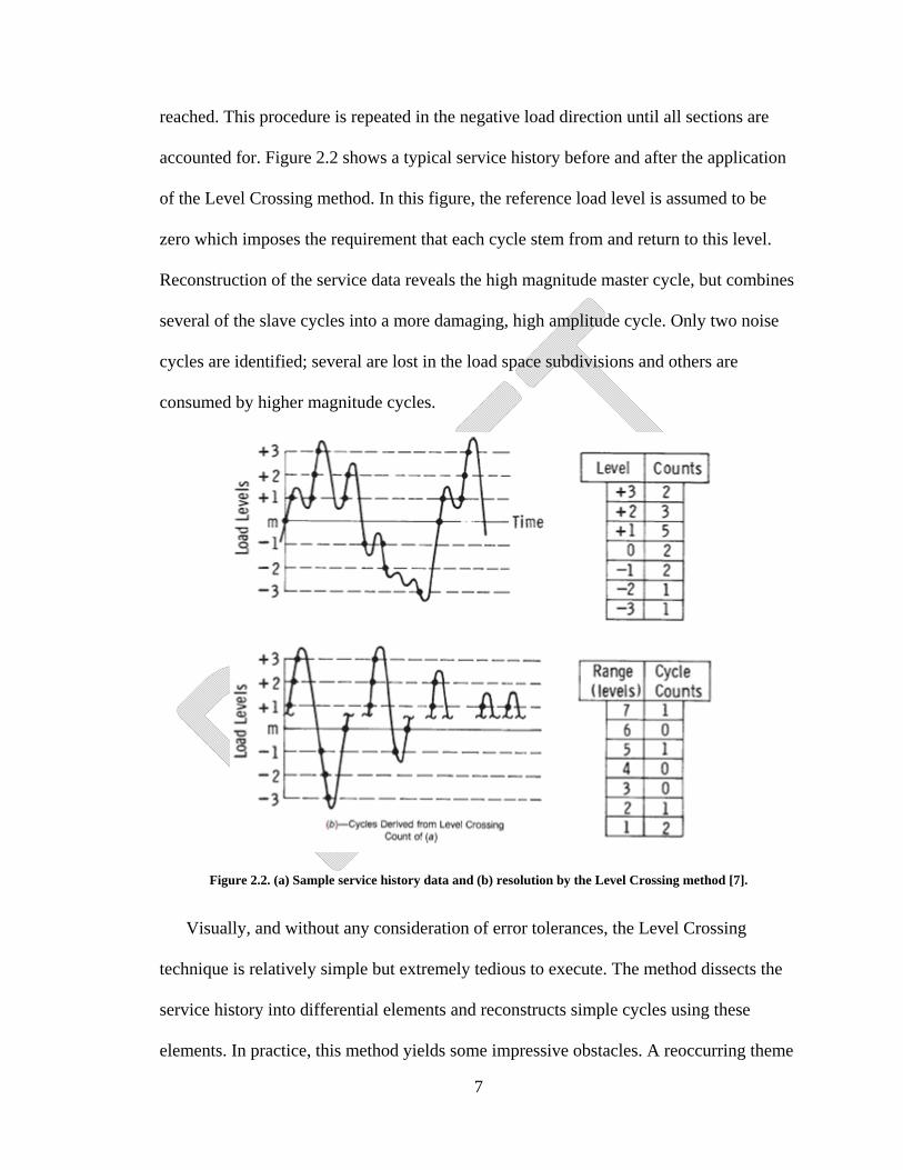
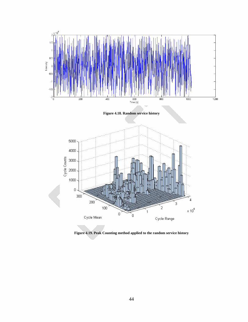
4.6 Random Cycling
The random cycling results exaggerate the underlying bivariate histogram trends
found in the specific signal simulations. Figure 4.18 shows a typical random service
history with upper and lower bounds of ±20,000 load units and a running average of zero
units. Figure 4.19 shows the result of the Peak Counting method on this load signal and
exhibits a trend on the mean-range plane. There is a clear sinusoidal oscillation of the
cycle mean along the range axis. Starting at zero range moving in the positive direction,
the cycle mean completes four quasi-sinusoidal cycles in the mean axis. The pattern is
likely caused by the nature of the service history; it is only quasi-random and has
artificial upper and lower imposed boundaries. The cycle count yielded by the peak
counting method is somewhat less conservative than in previous tests as many of the
reversal pairs do cross the reference level. Relative to methods that follow, the Peak
counting method still yields a conservative result.

43
The result of the Simple Range method applied to the random service history is
shown in Figure 4.20. Here a linear distribution along the range axis and a quasi-normal
distribution about the mean axis is exhibited. Again, this shape is likely a reflection of the
upper and lower-bounds imposed to the random number generator used to generate this
service history. Full range cycles swing from the lower-bound to the upper-bound limits,
which are symmetric similar to the distribution about the mean axis. This implies that a
full magnitude cycle must occur at or very near a zero mean.
The results of the Rain Flow method in Figure 4.21 exhibit more complex shapes
along the range and mean axis. Similar to the Simple Range method, a quasi-normal
distribution is observed along the mean axis but is also likely a reflection of the artificial
boundaries imposed on the random number generator used to produce this service
history. However, the range axis exhibits a quasi-Weibull distribution along the range
axis in combination with a higher number of full-range cycles. This result is a prime
example of the ability of the Rain Flow method to handle noise in an appropriate manner.
Although few statements can be made about the actual service history, it may be argued
that the full-range cycles have not been masked by noise, and noise has not been counted
as full-range cycles as with the Peak Counting method.
The RMS method summarizes the distribution from the Peak Counting method
with 164 counts at 261240 range and -8581 mean. Further study may be able characterize
the quality of this counting solution by estimating the damage yielded from this count
compared with that of the Rain Flow, Simple Range, and other counting methods.
44
Figure 4.18. Random service history
Figure 4.19. Peak Counting method applied to the random service history

45
Figure 4.20. Simple Range method applied to the random service history
Figure 4.21. Rain Flow method applied to random service history

46
4.7 Rate Handling
The latter phase of simulation in this research was the development and
evaluation of various rate extraction methods. This phase required that the scope of
evaluation be limited to a single, superior cycle counting method identified in previous
experimentation. Mentioned later, the algorithm selected was the ASTM Rain Flow
method for its ability to properly resolve load noise and unmask full-amplitude master
cycles. Further, these simulated experiments are conducted in three sub-phases: sub-
phase one evaluates a noise-free master cycle, sub-phase two evaluates combination
master-slave cycles to further exhibit issues in the extraction of rate parameters and sub-
phase three evaluates discontinuous, noisy cycles. To analyze the effects of noise, signals
from sub-phases one and two share a common master cycle of two load units in range and
a zero mean. Rates from all signals are extracted using the RRE, CFDA, and Linear LSR
methods defined in Chapter 3 (Equations 1-3) and shown in Figure 4.22.
Figure 4.22. Extraction method diagram
‐1.5
‐1
‐0.5
0
0.5
1
1.5
0 1 2 3
Service Value (arbitrary units)
Time (arbitrary units)
Value
Reversal Points
Linear Least SquaresRegression (LSR)
Reversal Rate Extraction(RRE)

47
4.8 Simple Signals
The goal of extracting rate parameters from any cycle is to summarize the load-
rate data in a single parameter that can be referenced along with range and mean
parameters to determine fatigue life for a given load event. The pivotal issue in this
scenario is that even simple, sinusoidal load signals exhibit rate data that is inherently
difficult to reduce to a single parameter. In Figure 4.23 the rate of a sinusoidal half-cycle
is summarized by the RRE, Linear LSR, and CFDA techniques. Visually, the linear LSR
method appears to best summarize the cycle rate by accounting for derivative dwell time;
the cycle rate is approximately constant for a large time frame near the center of the
cycle. Using the RRE method as a reference, the CFDA method yields a rate
approximately two percent faster. Similarly, the Linear LSR method yields a rate twenty
percent faster. Because the linear LSR method yields a higher rate for this type of signal,
this cycle type could potentially be cast as less damaging than if it had been analyzed
using the RRE or CFDA techniques [18]. Relative rate data is given in Figure 4.26.
Figure 4.23. Rate examination of a simple signal
4.9 Noisy Continuous Signals
The analysis of noisy continuous signals starts with the 2sum signal used in
previous sections. Figure 4.24 shows the half-cycle sample used for rate extraction

48
analysis. Using the RRE method as a reference, the CFDA technique only yields a
slightly higher cycle rate with a one percent increase. Similarly, the linear LSR method
yields a rate approximately twelve percent faster than the RRE method. This is likely due
to the statistical insignificance of the final points in the cycle which take a relatively
sharp turn in the positive load direction. Analyzing the underlying master cycle, the 2sum
signal yields virtually the same result when the RRE and CFDA methods are applied.
However, the LSR method yields a 6.2% decrease in extracted load rate, potentially
casting the common master cycle as more damaging compared to the simple signal.
Figure 4.24. Rate examination of the 2sum half-cycle
To further exhibit the effects of noise on cycle rate extraction, the 3sum signal
from Chapter 3 was analyzed using the three extraction methods. Compared with the
simple and 2sum results, this signal exhibits more closely grouped results. Again using
the RRE method as a reference, the CFDA method yields a rate 0.8% slower rate, and the
linear LSR method yields a 7.8% slower rate. Using the simple signal as a reference to
analyze the common master cycle, the RRE and CFDA methods both measure an
approximately 22% faster rate. In contrast, the linear LSR method measures a 5.2%
slower master cycle rate which again casts this cycle as potentially more damaging than
the RRE and CFDA methods.

49
Figure 4.25. Rate examination of the 3sum half-cycle
4.10 Relative Performance
The relative performance of the continuous signals and counting methods used in
sections 4.8-4.9 are shown in Figure 4.26Figure 4.27. Figure 4.26 utilizes the simple
signal as a reference rate. In this figure, the RRE and CFDA methods yield a sharply
increasing rate with increasing noise and complexity added into the master cycle. The
Linear LSR method yields a less distinct pattern, but exhibits the highest stability as it
extracts the master cycle rate within 6.2% of the actual rate. This may imply that the RRE
and CFDA methods could yield considerably less conservative damage estimates
compared with that of the Linear LSR method. However, the effect of noise on fatigue
life is outside of the scope of this research.
Figure 4.27 uses the RRE method as a reference for each signal. In this figure, the
CFDA method extracts a slightly higher rate (+1.9%) from the simple signal that
decreases with increasing complexity to reach a 0.8% slower rate. The linear LSR
initially extracts a 20% faster rate than the RRE method on the simple signal, but
decreases with increasing complexity to a 7.2% slower rate than the RRE method.

50
Figure 4.26. Relative extraction performance with increasing signal complexity (Simple signal reference)
Figure 4.27. Relative extraction performance (RRE method reference)
Simple 2sum 3sum
RRE 100.0% 100.0% 123.8%
CFDA 100.0% 99.2% 120.5%
LSR 100.0% 93.8% 94.8%
60.0%
70.0%
80.0%
90.0%
100.0%
110.0%
120.0%
130.0%
140.0%
Relative Rate
Simple 2sum 3sum
RRE 100.0% 100.0% 100.0%
CFDA 101.9% 101.1% 99.2%
LSR 120.3% 112.8% 92.2%
60.0%
70.0%
80.0%
90.0%
100.0%
110.0%
120.0%
130.0%
140.0%
Relative Rate

51
4.11 Discontinuous Load Signals
Sudden or discontinuous cycle events are commonly encountered in fatigue
analysis [1,3,10,13] and present a relatively complicated set of issues in cycle counting
and rate extraction. Figure 4.28 shows a pure step load event as identified by the Rain
Flow cycle counting method. Based on the cycle identification made by the Rain Flow
method, the cycle includes not only the cycle event, but an extended dwell time which is
not properly resolved. The inclusion of these dwell points causes considerable skewing of
the RRE, CFDA and linear LSR methods, which visually appear to be invalid. This
scenario represents the fundamental issue in handling discontinuous service events.
Further research in discontinuities and dwell handling may resolve problematic results
such as these.
Figure 4.28. Rate examination of a step cycle
A more realistic load signal shown in Figure 4.29 is a half-cycle from the
step2sum service history defined in Figure 4.1. Analysis of this signal cannot be applied
to make any comment about the underlying master cycle, because it has been severely
clipped and discretized to form a step function. Using the RRE method as a reference, the
CFDA method returns a 0.7% slower rate and the linear LSR returns a 5.2% slower rate
resulting in a cycle of potentially higher damage.

52
Figure 4.29. Rate examination of the step2sum half-cycle
4.12 Relative Performance
The relative performance of the RRE, CFDA, and Linear LSR methods are shown
in Figure 4.30 using the step signal as a reference. Upon visual inspection, the methods
extract rates that differ by considerable margins. However, this is a reflection of the cycle
window definition imposed by the Rain Flow cycle counting method used in this
experiment. Figure 4.28 shows the problematic cycle window resolved by this method.
Because the window includes the cycle dwell time, the rate is severely skewed to a lower
value which in turn will lead to a more conservative damage estimation. Until a
procedure for handling discontinuous service events is augmented to the existing Rain
Flow procedure, little conclusions can be drawn from these tests. Figure 4.31 shows the
relative performance of the rate extraction methods using the RRE method as a reference.
In this figure, the CFDA and Linear LSR methods extract significantly slower rates that
may lead to more conservative damage estimates using existing models. Because of the
limited data available, no conclusion can be drawn on extraction performance with
increasing complexity.

53
Figure 4.30. Relative extraction performance on discontinuous signals (step reference)
Figure 4.31. Relative extraction performance on discontinuous signals (RRE Reference)
4.13 Computational Performance
The cputime function in FORTRAN was utilized in the MACC program to
analyze basic computational expenses when running the top-level subroutines such as the
RRE CFDA LSR
Step 100.00% 100.00% 100.00%
Step2Sum 134.91% 156.92% 279.50%
0.00%
50.00%
100.00%
150.00%
200.00%
250.00%
300.00%
Relative Rate
RRE CFDA LSR
Step 100.0% 53.1% 29.8%
Step2Sum 100.0% 61.8% 61.8%
0.0%
20.0%
40.0%
60.0%
80.0%
100.0%
120.0%
Relative rate chage

54
function generator, reversal point resolution, and counting procedures. Data for this study
was generated using a basic IA-32 x86 hardware environment with the MACC executable
assigned its own thread affinity from the multi-core processor. This helped to eliminate
environment variables such as background threads and user interaction. Figure 4.32
shows the general trend of time requirements for each top-level subroutine to execute. A
characteristic of the Rain Flow method not previously exhibited in this research is its
growth rate; although the Rain Flow method executes in considerably shorter time, it
appears to grow at the same rate as the Peak Counting method. Figure 4.33 implies that
the number of operations required by the Rain Flow method as coded in the MACC
program grows in correlation with the square of the number of data points in the service
history.
Figure 4.32. CPU time used in MACC execution - Step input
1.00E‐03
1.00E‐02
1.00E‐01
1.00E+00
1.00E+01
1.00E+02
1.00E+03
1.00E+04
0 50 100 150 200
N ‐Thousands of data points
Function Generator
Reversal Point Resolution
Peak Counting
Rain Flow
Simple Range
RMS Method

55
Figure 4.33. CPU time used by Rain Flow method - 2sum signal
y = 3E‐08x2 + 0.0001x ‐ 0.0601
y = 3E‐07x2 ‐ 4E‐05x ‐ 0.0054
0
100
200
300
400
500
600
700
800
900
0 50 100 150 200
Run tim
e (s)
N ‐ number of data points
Thousands
Step Signal
2Sum Signal
Poly. (Step Signal)
Poly. (2Sum Signal)

56
5. Applications
The rate handling results from Chapter 4 were applied in three case studies to
simulate scenarios commonly found in industry [3,6,8,10]. As the results from Chapter 4
measured the effect of noise and secondary cycles on the rate extracted by the RRE,
CFDA, and Linear LSR methods, these case studies aim to observe their aggregate
performance in possible industrial applications. Using cycles counted by the Rain Flow
method, the RRE, CFDA, and Linear LSR methods are applied to three different
scenarios and the rate extraction results are represented by bivariate histograms as in
Chapter 4. In these plots, the engage and disengage rates are used as the variations and
the number of counts are plotted on the vertical axis. The results are summarized by the
unsigned engage and disengage rate means and 95% confidence intervals to represent the
statistical variety of rates that may be extracted in these scenarios.
5.1 Offshore Structures
The offshore structure test is intended to represent periods of calm and stormy
seas experienced by offshore structures such as oil rigs, pipelines, weather stations,
barges, and other structures subject to wind and waves. The service history sample shown
in Figure 5.1 has arbitrary scales about the time and amplitude axes and is plotted with
the reversal data resolved by the MACC program.

57
Figure 5.1. Offshore structure service history sample
The RRE extraction method results, shown in Figure 5.2, exhibit the majority of
the identified cycles engaging at relatively low rates (4.49 ± 7.26 units per second).
Because each cycle is roughly symmetric, the disengaging rates exhibit similar grouping
(5.79 ± 4.96 units per second). The CFDA extraction results (Figure 5.3) exhibit
engaging rates slightly higher and with similar grouping (6.05 ± 6.13 units per second).
Characteristic of the service history, the disengaging rates exhibit similar grouping (6.77
± 5.04 units per second).The Linear LSR extraction method results shown in Figure 5.4
yield similar engaging rates as the CFDA method (4.74 ± 7.73 units per second) and
disengaging rates (6.81 ± 6.86 units per second).
A comparison of these results is shown in Figure 5.5. Comparison of these results
does not yield any definitive conclusion about the various extraction methods. In this
service scenario, all three extraction methods yield closely grouped results. This is likely
attributable to the characteristics of the service history; the history does not contain any
major secondary signals or noise to skew the service history away from the lines (and
therefore, rates) that connect the reversal points (Figure 5.1).

58
Figure 5.2. RRE method applied the offshore service history
Figure 5.3. CFDA method applied to the offshore service history

59
Figure 5.4. Linear LSR method applied to the offshore service history
Figure 5.5. Extraction method comparison (offshore structure)
5.2 Land-based Structures
The land-based structure test is intended to represent primary cycles (i.e., the
weight rush hour traffic on a bridge), secondary cycles (i.e., the wheel of each vehicle
‐4
‐2
0
2
4
6
8
10
12
14
16
RRE Engage RREDisengage
CFDAEngage
CFDADisengage
LSR Engage LSRDisengage
Rate (units/sec)
Extraction Method
Average
95% CI Max
95% CI Min

60
passing) and noise (i.e., irregularities in the road surface and other vibrations). Figure 5.6
shows a sample of such a service history used in this test. Again, the data has semi-
arbitrary scales about the amplitude and time axes. Figure 5.7 shows a closer view of the
noise cycles contained in this history. The RRE extraction results (Figure 5.8) yield
engage rates of 38.48 ± 13.35 units per second and disengage rates of 54.93 ± 24.21 units
per second. The CFDA method returns similar rates of 30.02 ± 6.62 and 50.62 ± 26.06
units per second. The Linear LSR method yields engage and disengage rates centered at
approximately the same values of 37.90 and 55.67 units per second, respectively. In
contrast, the LSR method uncovers a much wider range of cycle rates both higher and
lower than that of the RRE and CFDA methods at ±40.25 and ±49.98 units per second,
respectively.
Comparison of these results (Figure 5.11) reveals that the mean of the rates
extracted by the three methods is approximately the same. However, the range of rates
extracted by the methods differs considerably when comparing the RRE and CFDA
methods to the Linear LSR method. In this scenario, the LSR method extracts rates 25%-
36% faster and slower than the RRE and CFDA methods. Although damage estimation is
outside the scope of this research, it appears that the Linear LSR method may yield
considerably different fatigue characteristics than that of the RRE and CFDA methods.
Further observation uncovers a potential issue with this data. As noted in Chapter 4,
discontinuities in the service history lead to miscalculation of cycle windows. This in turn
leads to asymmetric engaging and disengaging rates to be extracted from the skewed
windows. In this service history, the cycle windows are shifted forward in time leading to

61
increased engaging and decreased disengaging rates. This issue will be addressed in
further research.
Figure 5.6. Land-base structure service history sample
Figure 5.7. Secondary cycles from the Land-base structure service history

62
Figure 5.8. RRE extraction method applied to the land-based structure service history
Figure 5.9. CFDA extraction method applied to the land-based structure service history

63
Figure 5.10. Linear LSR extraction method applied to the land-based structure service history
Figure 5.11. Extraction method comparison (land-based structure)
5.3 Automotive Components
The automotive component test models the filtered torsional stresses in a high
performance sports car moving from a complete stop to top speed and back to a stop
‐20
0
20
40
60
80
100
120
RRE Engage RREDisengage
CFDAEngage
CFDADisengage
LSR Engage LSRDisengage
Rate (unit/sec)
Extraction Method
Average
95% CI Max
95% CI Min

64
under several repetitions. The test data includes the torque curve shapes from a typical
mid-displacement (3-4 Liters) I-6 engine with variable valve timing. Discontinuous steps
are also included by modeling gear shifts through a 6-speed automatic transmission. This
configuration yields secondary loading events and dwelling making it an ideal candidate
for rate extraction testing. The full service history (Figure 5.12) shows 15 sequential top-
speed runs with torque loads up to 4000 lb-ft. Observation of a single cycle (Figure 5.13)
reveals the challenges of extracting a meaningful rate from such a history. The cycle
definition imposed by the Rain Flow algorithm casts each run as a single cycle with
multiple discontinuities and dwells.
The RRE extraction method yields rates with very close grouping at 2960 ± 8.654
units per second engaging and 354.4 ± 0.1 units per second disengaging. This close
grouping is expected as each cycle is virtually identical. The CFDA extraction method
returns significantly higher engaging rates at 2945 ± 8.462 units per second and similar
disengaging rates at 433.9 ± 0.196 units per second. The Linear LSR method returns
engaging rates similar to that of the RRE method at 1862 ± 98.56 units per second but
significantly slower disengaging rates at 331.9 ± 0.991 units per second.
Because the engaging and disengaging rates vary by an order of magnitude, the
comparison plot was split into its respective halves. Comparison of the engaging rates
(Figure 5.17) shows the RRE and CFDA methods to return approximately identical
values. However, the Linear LSR method returns a 66% slower engaging rate which may
lead to more conservative damage estimations. In contrast, comparison of the
disengaging rates (Figure 5.18) shows the RRE and LSR methods returning an

65
approximately identical rate. The CFDA method returns a rate approximately 25% slower
that may be skewed by the discontinuities in the disengaging portion of the cycle.
Figure 5.12. Automotive axle service history
Figure 5.13. Single cycle from the automotive axle service history

66
Figure 5.14. RRE extraction method applied to the automotive axle service history
Figure 5.15. CFDA extraction method applied to the automotive axle service history

67
Figure 5.16. LSR extraction method applied to the automotive axle service history
Figure 5.17. Comparison of engaging rates (automotive)
0
500
1000
1500
2000
2500
3000
3500
RRE CFDA LSR
Rate (Units per second)
Extraction Method
Average
95% CI Max
95% CI Min

68
Figure 5.18. Comparison of disengaging rates (automotive)
0
50
100
150
200
250
300
350
400
450
500
RRE CFDA LSR
Rate (Units per Sec.)
Extraction Method
Average
95% CI Max
95% CI Min

69
6. CONCLUSIONS AND FUTURE WORK
6.1 Cycle Counting
This research involves the evaluation of the zero, single, and double parameters
cycle counting methods and documented their development into programmable
procedures. Analysis at the procedural level of these methods uncovers some significant
issues with the single parameter methods.
If the definition of cycle counting is to extract, process, and sort simple cycles
from a complex loading history, then it may be argued that the Level Crossing technique
is technically not a complete cycle counter. Although this procedure employs a unique
method to break down a service history at the load level (rather than the reversal level)
into discreet elements, the process only covers the reconstruction of simple cycles.
Although this yields simple cycles that can be counted visually, all load points are
accounted for in the reconstruction and visually counting long reconstructions is not
optimal. This method requires an additional counting procedure to reduce the data set into
counts. Because the reconstructed cycles oscillate about the reference load level and no
longer contain noise, the Peak Counting or Simple Range methods can be employed to
properly resolve the reconstructed load data.
The Peak Counting method mimics the intuitive procedure an operator may use to
count a simple service history visually. However, developing this process into a cycle
counting algorithm for use on complex service histories yields extremely conservative
results. Because this and other methods can only operate directly on reversal data, when
peaks below and above the reference load level are counted and sorted, noise is processed

70
as if it fulfills the fundamental assumptions made by this method; most notably, that all
reversal points stem and return to the reference load level. Further, this method employs
one of the most computationally intense routines found in numerical programming: value
sorting within an array. The culmination of these features reveals a highly conservative
method with high computational expense. However, this method could be employed to
establish a crude lower-bound on a confidence interval of service damage in further
research.
As the name implies, the Simple Range method is one of the simplest counting
procedures in that it does not require sorting, rearrangement, or intense processing of any
kind—ranges between reversals points are simply counted as half cycles. However, the
counting solution yielded from this method is highly sensitive to noise. If there are any
interruptions between master cycle reversal points, the method simply splits the cycle
into continuous, low-amplitude segments that are counted as half-cycles. From a cycle
counting perspective, this is highly erroneous. For any given complex service history, this
method may at best be employed as a lower bound for damage estimation.
The double parameter methods are aggregated to a single counting procedure in
this study as each of the methods performs the same underlying task masked by
variations in terminology. The Hayes, Range Pair, Ordered Overall Pair, Racetrack,
Hysteresis Loop, and Rainflow methods all operate on the basis of identification of
hysteresis loops in load data [7]. Although the computational expense of this method
grows at a similar rate as the Peak Counting method with the number of reversals to
process, it yields a robust counting solution that appears to be able to properly resolve all
continuous signal types.

71
6.2 Rate Handling
Of the rate extraction methods developed in this research, there does not appear to
be a clear and meaningful trend among the results that leads to the selection of a single
technique. Analyzing identical continuous master cycles with increasing noise and
secondary cycles, the LSR method exhibits the most stability; analyzing the Simple,
2sum, and 3sum signals sequentially reveals less than a 5% change in extracted rate by
the LSR method. In contrast, the RRE and CFDA methods exhibited excellent stability
on the 2sum signal with no noticeable change, but returned a 20% faster rate when
applied to the 3sum signal. Based on these results, it may be concluded that the LSR
method is the superior of the three techniques for extracting rate parameters from cycles
defined by the Rain Flow cycle counting technique.
Results from the analysis of discontinuous signals yield uncertain conclusions.
The CFDA and LSR methods returned rates up to 80% slower than that of the RRE
method on both pure and noisy step signals. Although the cycle definition was identical
throughout these tests, the effect of dwells and discontinuities in the service history are
handled in fundamentally different manners among the three extraction methods. The
issue of cycle definition in the presence of dwell and discontinuous periods along with
the fatigue life characteristics of these events needs to be addressed in further research
before any conclusion can be drawn about the performance of these extraction methods
on discontinuous signals.
The case studies reveal the aggregate performance of the extraction methods
developed in this paper in three possible industrial applications. For off-shore structures,
or perhaps any machine element or structure subject to relatively noise-free service of
variable amplitude may not benefit from any one particular method. The RRE, CFDA,

72
and Linear LSR methods yielded results too close to make a definitive distinction among
them. For land-based structures, or any component of interest subject to discontinuous,
noisy service histories with secondary cycles the LSR method appears to be able to
uncover a wider range of rates that may lead to more precise damage estimations. Further
research will determine the validity of the LSR method in this scenario. For some
automotive applications subject to relatively clean service histories with discontinuities it
appears that the Linear LSR method is adept to reveal the lowest (and perhaps most
damaging) cycle rates. Few definitive conclusions can be drawn from this test data with
respect to the RRE and CFDA methods.
6.3 Future Research
Concerning further development of the MACC code, there are three major facets that
may lead to more definitive conclusions in this research scope. First and foremost is code
refinement. Many of the computational expenses calculated by the MACC program are
merely products of the specific implementations used by the programmer. For instance, it
could be argued that the bubble-sort routine is the least efficient implementation of a
sorting algorithm found in literature [20]. This routine is included in the MACC program
due to its ease of implementation and short code length. A non-optimized sorting
algorithm is also present in the Rain Flow routine that grows at a similar rate. This raises
the question of whether the computational expenses calculated by the MACC program
reveal characteristics about the inner-workings of the cycle counting algorithms, or
merely their manifestations in the program.
Regarding the analysis of extracted rate parameters, the MACC program requires
additional development to handle discontinuous signals. The analysis of discontinuous

73
and dwelling signals from Chapter 4 and their application in Chapter 5 exhibit rates
heavily skewed by improper window definitions calculated by the Rain Flow algorithm.
Further development in the Rain Flow procedure and its implementation in the MACC
code may alleviate these issues.
Another facet of interest in further development is the creation of an upper and lower-
bound counts computed by the Simple Range and Peak Counting methods. In Chapters 2
and 3 these methods were characterized as highly-conservative and non-conservative,
respectively. Using these methods to develop upper and lower bound counts restates a
complex underlying issue mentioned in Chapter 4; reducing and summarizing this
information into a single parameter in a meaningful and consistent manner is neither
defined nor standardized. One proposed method is to pass the counting solutions to a
damage accumulation routine (such as Miner’s Rule) that returns the percentage of some
arbitrary (but standardized) standard service life consumed by the loading history. To
accomplish this, a set of standard fatigue properties and parameters would need to be
analyzed and established for various scenarios. This would create a standard framework
on which meaningful comparisons could be made among fatigue analysis elements such
as cycle counting and rate extraction.

APPENDIX A: SOURCE CODES

APPENDIX A.1: MACC PARENT MODULE (main.f90)
!-----------=[header]=----------- ! language: FORTRAN 90 ! format: free ! written by: ryan o'kelley ! version: alpha 1.0 !-------------------------------------------------------------------------------------- ! main program !-------------------------------------------------------------------------------------- program main !-------------------------------------------------------------------------------------- ! declare arguments !-------------------------------------------------------------------------------------- use subs !subroutines from 'subs.f90' use global !for commonly used arguments: 'global.f90' character*20 mode real zo1 !-------------------------------------------------------------------------------------- ! call stress history emulator subroutine to write stress.txt !-------------------------------------------------------------------------------------- mode = "simple" call stresswrite(mode) !-------------------------------------------------------------------------------------- ! data file and loading operations !-------------------------------------------------------------------------------------- !------------------------------------------------------ ! check and load parameters.txt !------------------------------------------------------ call params if (.not. go) goto 99 !------------------------------------------------------ ! check and load stress.txt !------------------------------------------------------ n_stress = 0 call check_stress if (.not. go) goto 99 call load_stress !------------------------------------------------------ ! check and load snr surface !------------------------------------------------------ call snrload !-------------------------------------------------------------------------------------- ! cycle counting !-------------------------------------------------------------------------------------- !------------------------------------------------------ ! count and load local maxima and minima of stress history !------------------------------------------------------ local = 0 n_local = 0 go = .false. call stress_peak if (.not. go) goto 99 !------------------------------------------------------ ! Peak Counting !------------------------------------------------------ if (pc_flag == 1)call peak_count !------------------------------------------------------ ! rainflow !------------------------------------------------------ if (rf_flag == 1)call rainflow(local,n_local) !------------------------------------------------------ ! Simple Range !------------------------------------------------------ if (sr_flag == 1)call simple_range(local,n_local) !------------------------------------------------------ ! rms !------------------------------------------------------

76
if (rms_flag == 1)call rms_count !-------------------------------------------------------------------------------------- ! debug !-------------------------------------------------------------------------------------- print *,'debug' print *,'s--------------------------' print *,ss print *,'n--------------------------' print *,nn print *,'r--------------------------' print *,rr print *,'end debug' !------------------------------------------------------ ! pause, end main program !------------------------------------------------------ 99 pause end program main !-------------------------------------------------------------------------------------- ! end of main program !--------------------------------------------------------------------------------------

77
APPENDIX A.2: MACC GLOBAL NAMESPACE MODULE (global.f90)
!-------------------------------------------------------------------------------------- ! global storage module !-------------------------------------------------------------------------------------- module global implicit none !subroutine error flag logical go !runtime parameters integer rf_flag, pc_flag, sr_flag, rms_flag !1 = on, 0 = off character*256 :: stress_path, output_dir character*32 :: ratemode ! service history real, dimension(:,:), allocatable :: stress integer n_stress ! local stress peaks real, dimension(:,:), allocatable :: local integer n_local !s-n-r surface real, dimension(:), allocatable :: ss real, dimension(:,:), allocatable :: nn real, dimension(:), allocatable :: rr integer n_s, n_n, n_r ! used by rms and Peak Counting subroutines real, dimension(:,:), allocatable :: peak_max, peak_min ! used by rms real avg ! used by rainflow real, dimension(:,:), allocatable :: rain integer n_rain end module global !-------------------------------------------------------------------------------------- ! end of global storage module !--------------------------------------------------------------------------------------

78
APPENDIX A.3: MACC SUBROUTINE MODULE (subs.f90)
!-------------------------------------------------------------------------------------- ! module for subroutines used in 'sfd.f90' !-------------------------------------------------------------------------------------- module subs implicit none contains !-------------------------------------------------------------------------------------- ! load paramters from gui !-------------------------------------------------------------------------------------- subroutine params use global !for counter flags and parameters integer length, i logical para_exist character*256 dummy go = .false. !------------------------------------------------------ ! inquire parameter file !------------------------------------------------------ print *,"inquiring parameters.txt" inquire(file="input/parameters.txt",exist=para_exist) !------------------------------------------------------ ! end subroutine if parameters.txt not found !------------------------------------------------------ if(.not. para_exist) then print *,"error--parameter file (parameters.txt) not found! abandon ship!" goto 89 else print *,"parameters.txt found!" endif !------------------------------------------------------ ! open and check parameter file !------------------------------------------------------ open(unit=19,file="input/parameters.txt",form="formatted",action="read",status="old") do i = 1,4 read(19,*) enddo read(19,'(A)') dummy if (trim(dummy) == "MAAC GUI Ver: 0.0") then print *,"gui is ok!" read(19,'(A)') dummy if (trim(dummy) == "MAAC Console Ver: 1.1 alpha") then print *,"parameter file is ok!" go = .true. else print *,"error--parameter file is not compatible! abandon ship!" goto 89 endif else print *,"error--gui program is not compatible! abandon ship!" goto 89 endif rewind(19) !------------------------------------------------------ ! read service history path !------------------------------------------------------ do i = 1,7 !skip lines read(19,*) dummy enddo backspace(19) !backup read(19,'(A)') stress_path !read length = len(stress_path) !trim stress_path = stress_path(13:length)!trim length = 0 !reset

79
!------------------------------------------------------ ! read output path !------------------------------------------------------ read(19,*) dummy !skip do i = 1,1 !backup backspace(19) enddo read(19,'(A)') output_dir !read length = len(output_dir) !trim output_dir = output_dir(14:length) !trim !------------------------------------------------------ ! read counter flags !------------------------------------------------------ !rainflow read(19,*) dummy !advance backspace(19) !rewind read(19,'(A)') dummy !read dummy = dummy(21:21) !trim rf_flag = ichar(dummy) !convert to integer rf_flag = rf_flag - 48 !translate ascii value !Peak Counting !repeat read(19,'(A)') dummy dummy = dummy(21:21) pc_flag = ichar(dummy) pc_flag = pc_flag - 48 !Simple Range read(19,'(A)') dummy dummy = dummy(21:21) sr_flag = ichar(dummy) sr_flag = sr_flag - 48 !rms read(19,'(A)') dummy dummy = dummy(21:21) rms_flag = ichar(dummy) rms_flag = rms_flag - 48 89 end subroutine params !-------------------------------------------------------------------------------------- ! end of parameter loading !-------------------------------------------------------------------------------------- !-------------------------------------------------------------------------------------- ! stress history text file checking subroutine !-------------------------------------------------------------------------------------- subroutine check_stress !------------------------------------------------------ ! declare arguments !------------------------------------------------------ use global !for n_stress and stress array logical stress_exist integer i, io !------------------------------------------------------ ! check for stress text file !------------------------------------------------------ go = .false. print *,"inquiring stress.txt" inquire(file=trim(stress_path),exist=stress_exist) !------------------------------------------------------ ! end subroutine if stress.txt not found !------------------------------------------------------ if(.not. stress_exist) then print *,"error--stress history file (stress.txt) not found! abandon ship!" goto 97 else print *,"stress.txt found!" endif !------------------------------------------------------ ! check number of lines in stress.txt

80
!------------------------------------------------------ open(unit=11,file=trim(stress_path),form="formatted",action="read",status="old") io = 0 i = 0 do while (io == 0) read(11,*,iostat=io) i = i + 1 end do i = i - 1 n_stress = i print *,n_stress,' stress records found!' !------------------------------------------------------ ! end program if stress.txt is empty !------------------------------------------------------ if (i == 0) then print *,"error--stress history file (stress.txt) is empty! abandon ship!" call print_div goto 97 else go = .true. endif !------------------------------------------------------ ! done with stress.txt !------------------------------------------------------ close (11) !------------------------------------------------------ ! end subroutine !------------------------------------------------------ 97 end subroutine check_stress !-------------------------------------------------------------------------------------- ! end of stress history text file checking subroutine !-------------------------------------------------------------------------------------- !-------------------------------------------------------------------------------------- ! s-n-r surface loading !-------------------------------------------------------------------------------------- subroutine snrload use global !for s, n, and r arrays integer i, j, io open(unit=22,file='input/snr/sf.txt',form="formatted",action="read",status="old") io = 0 i = 0 do while (io == 0) read(22,*,iostat=io) i = i + 1 end do i = i - 1 n_s = i allocate(ss(n_s)) rewind(22) do i = 1,n_s read(22,*) ss(i) enddo close(22) open(unit=24,file='input/snr/r.txt',form="formatted",action="read",status="old") io = 0 i = 0 do while (io == 0) read(24,*,iostat=io) i = i + 1 end do

81
i = i - 1 n_r = i allocate(rr(n_r)) rewind(24) do i = 1,n_r read(24,*) rr(i) enddo close(24) open(unit=23,file='input/snr/n.txt',form="formatted",action="read",status="old") allocate(nn(n_r,n_s)) do i = 1,n_s do j = 1,n_r read(23,*) nn(j,i) enddo enddo close(23) end subroutine snrload !-------------------------------------------------------------------------------------- ! stress array loading subroutine !-------------------------------------------------------------------------------------- subroutine load_stress !------------------------------------------------------ ! declare arguments !------------------------------------------------------ use global !for n_stress and stress array integer i !------------------------------------------------------ ! load stress.txt !------------------------------------------------------ print *,"allocating memory to stress array" allocate (stress(n_stress,4)) open(unit=12,file=trim(stress_path),form="formatted",action="read",status="old") do i=1,n_stress read(12,*) stress(i,1),stress(i,2) enddo print *,"stress history succesfully loaded!" close (12) !------------------------------------------------------ ! end subroutine !------------------------------------------------------ 95 end subroutine load_stress !-------------------------------------------------------------------------------------- ! end of stress array loading subroutine !-------------------------------------------------------------------------------------- !-------------------------------------------------------------------------------------- ! stress history local maxima and minima subroutine !-------------------------------------------------------------------------------------- subroutine stress_peak !------------------------------------------------------ ! declare arguments !------------------------------------------------------ use global !for 'n_local' and 'local' array integer i,k,s1,s2 real val, last, now, next, t1, t2 !------------------------------------------------------ ! append 1st derivate to 'stress' array (finite difference, central) !------------------------------------------------------ call cpu_time(t1) !start timer

82
print*,"finding load rates" stress(1,3) = 0 !start of array stress(n_stress,3) = 0 !end of array do i=2,(n_stress-1) val = (stress(i+1,2) - stress(i-1,2)) / (stress(i+1,1) - stress(i-1,1)) stress(i,3) = val enddo open(unit=21,file="output/stressrate.txt",form="formatted",action="readwrite",status="replace") do i=1,n_stress write(21,*) stress(i,3) enddo !------------------------------------------------------ ! find local maxima and minima, append flags to stress array !------------------------------------------------------ print*,"finding peaks" k = 0 do i=2,(n_stress-1) last = stress(i-1,2) now = stress(i,2) next = stress(i+1,2) !typical conditionals if (last > now .and. next > now) then stress(i,4) = 1 k = k + 1 elseif (last < now .and. next < now) then stress(i,4) = 1 k = k + 1 !step function statements elseif (last == now .and. next < now) then stress(i,4) = 1 k = k + 1 elseif (last == now .and. next > now) then stress(i,4) = 1 k = k + 1 !elseif (last > now .and. next == now) then ! stress(i,4) = 1 ! k = k + 1 !elseif (last < now .and. next == now) then ! stress(i,4) = 1 ! k = k + 1 !no peak else stress(i,4) = 0 endif enddo n_local = k if (n_local == 0) then print*,"error, no peaks found in stress.txt! abandon ship!" goto 96 else go = .true. endif k = 1 !------------------------------------------------------ ! create local array !------------------------------------------------------ allocate(local(n_local,3)) do i=2,(n_stress-1) if(stress(i,4) == 1) then local(k,1) = stress(i,1) local(k,2) = stress(i,2) local(k,3) = i k = k + 1 endif enddo !------------------------------------------------------ ! write local array to local.txt !------------------------------------------------------ print*,"writing local array to local.txt"

83
call cpu_time(t2) !stop stimer print*,"operation finished in ",t2-t1," seconds" !report time call print_div open(unit=13,file="output/local.txt",form="formatted",action="readwrite",status="replace") do i=1,n_local write(13,*) local(i,1) , local(i,2) enddo !------------------------------------------------------ ! end subroutine !------------------------------------------------------ 96 end subroutine stress_peak !-------------------------------------------------------------------------------------- ! end of stress history local maxima and minima counting subroutine !-------------------------------------------------------------------------------------- !-------------------------------------------------------------------------------------- ! stress history average !-------------------------------------------------------------------------------------- subroutine average(array,n) use global !for avg integer i, n real sum, array(n) sum = 0 do i=1,n sum = sum + array(i) enddo avg = sum/n end subroutine average !-------------------------------------------------------------------------------------- ! end of stress history average !-------------------------------------------------------------------------------------- !-------------------------------------------------------------------------------------- ! Peak Counting subroutine !-------------------------------------------------------------------------------------- subroutine peak_count !------------------------------------------------------ ! declare arguments !------------------------------------------------------ use global !for peak_max and peak_min integer n_max, n_min, i, j, k, index, n, n_cycle real local_copy(n_local,2), ref, mag, max, min, delta, t1, t2 real, dimension(:,:), allocatable :: peak !------------------------------------------------------ ! set reference level and minimum cycle amplitude !------------------------------------------------------ call cpu_time(t1) !start timer print *,"counting cycles via: --Peak Counting--" ref = 0 do i=1,n_local ref = ref + local(i,2) !sum stress values enddo ref = ref/n_local !reference level = average of stress values delta = 10.0**-9 !ignore cycles less than delta print *,"reference level set at", ref print *,"ignoring cycles magnitudes under",delta !------------------------------------------------------ ! count number of maximums above reference level !------------------------------------------------------ print *," phase one" k = 0 !max counter

84
max = 1 !to pass while condition local_copy = local do while (abs(max - ref) > delta) call find_max(local_copy(:,2), n_local, max, index, ref) local_copy(index,2) = ref k = k + 1 enddo n_max = k - 1 !------------------------------------------------------ ! dump maximums to array !------------------------------------------------------ print *," phase two" allocate(peak_max(n_max,2)) k = 1 !array indexer max = 1 !to pass while condition local_copy = local !reset local_copy array do while (abs(max-ref) > delta) call find_max(local_copy(:,2), n_local, max, index, ref) local_copy(index,2) = ref if (k <= n_max) then peak_max(k,1) = local(index,1) peak_max(k,2) = max k = k + 1 endif enddo !------------------------------------------------------ ! count number of minimums below reference level !------------------------------------------------------ print *," phase three" k = 0 !reset index min = -1 !to pass while condition do while (abs(min-ref) > delta) call find_min(local_copy(:,2), n_local, min, index, ref) local_copy(index,2) = ref k = k + 1 enddo n_min = k - 1 !------------------------------------------------------ ! dump minimums to array !------------------------------------------------------ print *," phase four" allocate(peak_min(n_min,2)) k = 1 !array indexer min = 1 !to pass while condition local_copy = local !reset local_copy array do while (abs(min-ref) > delta) call find_min(local_copy(:,2), n_local, min, index, ref) local_copy(index,2) = ref if (k <= n_min) then peak_min(k,1) = local(index,1) peak_min(k,2) = min k = k + 1 endif enddo !------------------------------------------------------ ! combine maximums and minimums to form cycles !------------------------------------------------------ print *," phase five" if (n_max <= n_min) then n = n_max elseif (n_max > n_min) then n = n_min endif allocate(peak(n,3)) do i=1,n peak(i,1) = ( abs(ref - peak_max(i,2)) + abs(ref - peak_min(i,2)) ) !cylce amplitude peak(i,2) = (peak_max(i,2) + peak_min(i,2)) / 2. !cycle mean peak(i,3) = peak(i,1) / abs(peak_max(i,1) - peak_min(i,1)) !cycle rate

85
enddo print *,"counted",n,"cycles!" call cpu_time(t2) print *,"operation completed in ",t2-t1," seconds" !------------------------------------------------------ ! write cycles to file !------------------------------------------------------ open(unit=14,file="output/peak_counting.txt",form="formatted",action="readwrite",status="replace") write(14,*) " range" , " mean" , " rate" do i = 1,n write(14,*) peak(i,1) ,",", peak(i,2) ,",", peak(i,3) enddo close (14) !------------------------------------------------------ ! print results to file !------------------------------------------------------ print *,"printing cycle counting results to peak_counting.txt" call print_div !------------------------------------------------------ ! end subroutine !------------------------------------------------------ end subroutine peak_count !-------------------------------------------------------------------------------------- ! end of Peak Counting subroutine !-------------------------------------------------------------------------------------- !-------------------------------------------------------------------------------------- ! array maximum subroutine !-------------------------------------------------------------------------------------- subroutine find_max(array, n_array, max, index, ref) !------------------------------------------------------ ! declare arguments !------------------------------------------------------ integer i, j, k, index, n_array real array(n_array), ref, max, old !------------------------------------------------------ ! find max of array above ref !------------------------------------------------------ max = ref do i=1,n_array if (array(i) > max) then max = array(i) index = i endif enddo end subroutine find_max !-------------------------------------------------------------------------------------- ! end of array maximum subroutine !-------------------------------------------------------------------------------------- !-------------------------------------------------------------------------------------- ! array minimum subroutine !-------------------------------------------------------------------------------------- subroutine find_min(array, n_array, min, index, ref) !------------------------------------------------------ ! declare arguments !------------------------------------------------------ integer i, j, k, index, n_array real array(n_array), ref, min !------------------------------------------------------ ! find max of array above ref !------------------------------------------------------ min = ref

86
do i=1,n_array if (array(i) < min) then min = array(i) index = i endif enddo end subroutine find_min !-------------------------------------------------------------------------------------- ! end of array maximum subroutine !-------------------------------------------------------------------------------------- !-------------------------------------------------------------------------------------- ! rainflow counting subroutine !-------------------------------------------------------------------------------------- subroutine rainflow(array,n_array) !------------------------------------------------------ ! declare argumaents !------------------------------------------------------ use global !for rain array, n_rain, and ratemode logical stp integer i,j,k,n_array,indx(n_array),trash real x,y,mean,load_rate,unload_rate,array(n_array,3),t1,t2 !real, dimension(:,:), allocatable :: rain !uncomment this line to use w/o global module !------------------------------------------------------ ! header !------------------------------------------------------ print *,"counting cycles via: --rainflow--" call cpu_time(t1) !------------------------------------------------------ ! create index array !------------------------------------------------------ do i=1,n_array indx(i) = i end do !------------------------------------------------------ ! count number of cycles !------------------------------------------------------ print *," phase one" stp = .false. !to initially pass while condition n_rain = 0 !cycle counter i = indx(1) !initialize indices j = indx(2) k = indx(3) do while (.not. stp .and. k <= n_array) y = abs(array(i,2) - array(j,2)) x = abs(array(j,2) - array(k,2)) if (x >= y) then indx(i) = -1 !throws out indices with peaks indx(j) = -1 !throws out indices with peaks call indxld(i,j,k,indx,n_array,stp) n_rain = n_rain + 1 else i = j j = k call k_indxld(i,j,k,indx,n_array,stp) endif enddo !------------------------------------------------------ ! re-create index array !------------------------------------------------------ do i=1,n_array indx(i) = i end do !------------------------------------------------------ ! write cycles to array !------------------------------------------------------ print *," phase two"

87
allocate (rain(n_rain,9)) stp = .false. !to initially pass while condition n_rain = 1 !reset to array indexer i = indx(1) !initialize indices j = indx(2) k = indx(3) do while (.not. stp .and. k <= n_array) y = abs(array(i,2) - array(j,2)) x = abs(array(j,2) - array(k,2)) mean = (array(i,2) + array(j,2)) / 2. load_rate = y / (array(j,1) - array(i,1)) unload_rate = x / (array(k,1) - array(j,1)) if (x >= y) then rain(n_rain,1) = y rain(n_rain,2) = mean rain(n_rain,3) = load_rate rain(n_rain,4) = unload_rate rain(n_rain,5) = array(i,3) rain(n_rain,6) = array(j,3) rain(n_rain,7) = array(k,3) rain(n_rain,8) = -0. rain(n_rain,9) = -0. indx(i) = -1 !throws out indices with peaks indx(j) = -1 !throws out indices with peaks call indxld(i,j,k,indx,n_array,stp) n_rain = n_rain + 1 else i = j j = k call k_indxld(i,j,k,indx,n_array,stp) endif enddo n_rain = n_rain - 1 !------------------------------------------------------ ! compute rate data !------------------------------------------------------ ratemode = "wavg" call getrate(ratemode) !fills in rain(:,7) !------------------------------------------------------ ! report status !------------------------------------------------------ print *,"found",n_rain,"cycles" call cpu_time(t2) print *,"operation completed in ",t2-t1," seconds" print *,"printing cycle counting results to rain.txt" open(unit=15,file="output/rain.txt",form="formatted",action="readwrite",status="replace") write(15,*) " range mean rate" do i=1,n_rain write(15,*) rain(i,1), rain(i,2), rain(i,8),rain(i,9) enddo close(15) call print_div !------------------------------------------------------ ! end subroutine !------------------------------------------------------ end subroutine rainflow !-------------------------------------------------------------------------------------- ! end of rainflow counting subroutine !-------------------------------------------------------------------------------------- !-------------------------------------------------------------------------------------- ! index loader subroutine for rainflow !-------------------------------------------------------------------------------------- subroutine indxld(i,j,k,indx,n,stp) !------------------------------------------------------

88
! declare arguments !------------------------------------------------------ logical stp integer i,j,k,c,n,indx(n) !------------------------------------------------------ ! load next elements greater than zero !------------------------------------------------------ !------------------------------------------------------ ! load i !------------------------------------------------------ stp = .false. do c=1,n if (indx(c) > 0) then i = indx(c) goto 93 endif enddo 93 continue !------------------------------------------------------ ! load j !------------------------------------------------------ do c=i+1,n if (indx(c) > 0) then j = indx(c) goto 92 endif enddo 92 continue !------------------------------------------------------ ! load k !------------------------------------------------------ do c=j+1,n if (indx(c) > 0) then k = indx(c) goto 91 endif enddo 91 continue !------------------------------------------------------ ! stop if i = k (end of array) !------------------------------------------------------ if (i == k) stp = .true. !------------------------------------------------------ ! end subroutine !------------------------------------------------------ end subroutine indxld !-------------------------------------------------------------------------------------- ! end of index loader subroutine for rainflow !-------------------------------------------------------------------------------------- !-------------------------------------------------------------------------------------- ! index loader subroutine for rainflow !-------------------------------------------------------------------------------------- subroutine k_indxld(i,j,k,indx,n,stp) !------------------------------------------------------ ! declare arguments !------------------------------------------------------ logical stp integer i,j,k,c,n,indx(n) !------------------------------------------------------ ! load next k-element greater than zero !------------------------------------------------------ stp = .false. !------------------------------------------------------ ! load k !------------------------------------------------------ do c=j+1,n if (indx(c) > 0) then

89
k = indx(c) goto 91 endif enddo 91 continue !------------------------------------------------------ ! stop if i = k (end of array) !------------------------------------------------------ if (i == k) stp = .true. !------------------------------------------------------ ! end subroutine !------------------------------------------------------ end subroutine k_indxld !-------------------------------------------------------------------------------------- ! end of index loader subroutine for rainflow !-------------------------------------------------------------------------------------- !-------------------------------------------------------------------------------------- ! Simple Range counting subroutine !-------------------------------------------------------------------------------------- subroutine simple_range (array,n_array) !------------------------------------------------------ ! declare arguments !------------------------------------------------------ integer i,n_array real array(n_array,2),x,y,range,mean,rate,tx,ty,t1,t2 !------------------------------------------------------ ! find ranges, means and rates between all points !------------------------------------------------------ open(unit=16,file="output/simple_range.txt",form="formatted",action="readwrite",status="replace") write(16,*) " range ","mean ","rate" print *,"counting cycles via: --Simple Range--" call cpu_time(t1) do i=1,n_array-1 x = array(i,2) tx = array(i,1) y = array(i+1,2) ty = array(i+1,1) range = abs(y - x) mean = (x + y) / 2. rate = range / (ty - tx) write(16,*) range ,",", mean ,",", rate enddo close(16) print *,"found",int((n_array-1)/2.),"cylces" call cpu_time(t2) print *,"operation completed in ",t2-t1," seconds" print *,"printing cycle counting results to simple_range.txt" call print_div !------------------------------------------------------ ! end subroutine !------------------------------------------------------ end subroutine simple_range !-------------------------------------------------------------------------------------- ! end of Simple Range counting subroutine !-------------------------------------------------------------------------------------- !-------------------------------------------------------------------------------------- ! rms mehod - astm stp 748 !-------------------------------------------------------------------------------------- subroutine rms_count !------------------------------------------------------ ! declare arguments

90
!------------------------------------------------------ use global !for peak_max and peak_min integer i, n_max, n_min, n_rms real avg_max, avg_min, rms_max, rms_min, rms_range, dummy, t1, t2 !------------------------------------------------------ ! header !------------------------------------------------------ print *,"counting cycles via --rms--" call cpu_time(t1) !------------------------------------------------------ ! find array size !------------------------------------------------------ n_max = size(peak_max,1) n_min = size(peak_min,1) !------------------------------------------------------ ! find rms of maximums !------------------------------------------------------ print *," phase one" dummy = 0 do i=1,n_max dummy = dummy + peak_max(i,2)**2. enddo dummy = dummy/n_max dummy = sqrt(dummy) rms_max = dummy !------------------------------------------------------ ! find rms of minimums !------------------------------------------------------ print *," phase two" dummy = 0 do i=1,n_min dummy = dummy + peak_min(i,2)**2. enddo dummy = dummy/n_min dummy = sqrt(dummy) rms_min = dummy !------------------------------------------------------ ! find average of maximums !------------------------------------------------------ print *," phase three" dummy = 0 do i=1,n_max dummy = dummy + peak_max(i,2) enddo dummy = dummy/n_max avg_max = dummy !------------------------------------------------------ ! find average of minumums !------------------------------------------------------ print *," phase four" dummy = 0 do i=1,n_min dummy = dummy + peak_min(i,2) enddo dummy = dummy/n_min avg_min = dummy !------------------------------------------------------ ! transfer signs of averages to minimums !------------------------------------------------------ rms_max = sign(rms_max,avg_max) rms_min = sign(rms_min,avg_min) !------------------------------------------------------ ! declare rms range and number of cycles !------------------------------------------------------ rms_range = abs(rms_max - rms_min) n_rms = n_local/2 !------------------------------------------------------ ! write rms cycles to text file !------------------------------------------------------ print *,"counted",n_rms,"cycles at range",rms_range call cpu_time(t2)

91
print *,"operation completed in ",t2-t1," seconds" print *,"writing cycles to rms.txt" open(unit=18,file="output/rms.txt",form="formatted",action="readwrite",status="replace") write(18,*) "cycle range" do i=1,n_rms write(18,*) rms_range, avg !avg pulled from global, produced by 'average' sub enddo close(18) call print_div !------------------------------------------------------ ! end subroutine !------------------------------------------------------ end subroutine rms_count !-------------------------------------------------------------------------------------- ! end of rms method subroutine !-------------------------------------------------------------------------------------- !-------------------------------------------------------------------------------------- ! rms method - typical !-------------------------------------------------------------------------------------- subroutine rms_count2 !------------------------------------------------------ ! declare arguments !------------------------------------------------------ use global !for stress array and n_stress value integer i, n_rms real sumsq, rms, t1, t2 !------------------------------------------------------ ! find rms of load signal !------------------------------------------------------ print *,"counting cycles via --rms--" call cpu_time(t1) sumsq = 0 do i = 1,n_stress sumsq = sumsq + stress(i,2)**2. enddo rms = sqrt(sumsq/n_stress) n_rms = n_stress/2 print *,"counted",n_rms,"cycles at range",rms call cpu_time(t2) print *,"operation completed in ",t2-t1," seconds" print *,"writing cycles to rms.txt" open(unit=23,file="output/rms2.txt",form="formatted",action="readwrite",status="replace") write(23,*) "cycle range" do i=1,n_rms write(23,*) rms, avg !avg pulled from global, produced by 'average' sub enddo close(23) call print_div !------------------------------------------------------ ! end subroutine !------------------------------------------------------ end subroutine rms_count2 !-------------------------------------------------------------------------------------- ! end of rms method subroutine !-------------------------------------------------------------------------------------- !-------------------------------------------------------------------------------------- ! cycle rate handling subroutine

92
!-------------------------------------------------------------------------------------- subroutine getrate(mode) use global !to get rain and stress arrays integer i1, i2, i3, i, j, n real avrg, xavrg, yavrg, sumx, sumy, sumxx, sumxy, ls_slope character*20, intent(in):: mode if (trim(mode) == "avg") then avrg = 0. do i = 1,(n_rain) i1 = rain(i,5) !i i2 = rain(i,7) !k !take average, append to rain array do j = i1,i2 avrg = avrg + abs(stress(j,3)) enddo avrg = avrg/(i2-i1+1) rain(i,8) = avrg avrg = 0. enddo endif if (trim(mode) == "wavg") then sumx = 0. sumy = 0. sumxx = 0. sumxy = 0. do i = 1,(n_rain) i1 = rain(i,5) !i i2 = rain(i,6) !j i3 = rain(i,7) !k !find least squares slope from i to j do j = i1,i2 n = i2-i1+1 sumx = sumx + stress(j,1) sumy = sumy + stress(j,2) sumxx = sumxx + (stress(j,1))**2 sumxy = sumxy + stress(j,1)*stress(j,2) enddo xavrg = sumx/(n) yavrg = sumy/(n) ls_slope = (sumxy - sumx*yavrg) / (sumxx - sumx*xavrg) rain(i,8) = ls_slope !reset sumx = 0. sumy = 0. sumxx = 0. sumxy = 0. !find least squares slope from j to k do j = i2,i3 n = i3-i2+1 sumx = sumx + stress(j,1) sumy = sumy + stress(j,2) sumxx = sumxx + (stress(j,1))**2 sumxy = sumxy + stress(j,1)*stress(j,2) enddo xavrg = sumx/(n) yavrg = sumy/(n) ls_slope = (sumxy - sumx*yavrg) / (sumxx - sumx*xavrg) rain(i,9) = ls_slope !reset sumx = 0 sumy = 0 sumxx = 0 sumxy = 0 enddo endif end subroutine getrate

93
!-------------------------------------------------------------------------------------- ! end of cycle rate handling subroutine !-------------------------------------------------------------------------------------- !-------------------------------------------------------------------------------------- ! stress history emulator subroutine !-------------------------------------------------------------------------------------- subroutine stresswrite(func) use global character*20 func, mode integer slave real s,pi,f,w,mag,val, t1, t2, i, dt, max parameter (dt = 0.001) parameter (max = (10)/10. + .006) !number in brackets is the number of master cycles call cpu_time(t1) !start clock print *,"emulating stress history" print *,"mode is set to: ",func open(unit=11,file="input/stress.txt",form="formatted",action="readwrite",status="replace") i = 0 do while (i <= max) !i = time (s) call funcgen(i,func,val) if (.not. go) goto 90 write(11,*) i,val i = i + dt enddo call cpu_time(t2) print *,"operation finished in ",t2-t1," seconds" call print_div close (11) 90 end subroutine stresswrite !-------------------------------------------------------------------------------------- ! end of stress history emulator subroutine !-------------------------------------------------------------------------------------- !-------------------------------------------------------------------------------------- ! function generator !-------------------------------------------------------------------------------------- subroutine funcgen(x,f,y) use global character*20, intent(in) :: f real, intent(out) :: y real, intent(in) :: x real dt parameter (dt = .003) real j,fq,pi,w,trash integer slave, offset parameter(fq = 10., & !frequency pi = 3.14159265358979323846, & !pi w = 2*pi*fq, & !angular argument for periodic functions (omega) slave = 10 ) !number of slave cycles per master cycle go = .false.
94
if (f == "simple") then y = cos(w*(x-dt)) go = .true. elseif (f == "2sum") then y = cos(w*(x-dt)) + (1./8.)*cos(slave*w*(x-dt)) go = .true. elseif (f == "3sum") then !first term is a super-master cycle y = cos(w/slave*(x-dt)) + (1./4.)*cos(w*(x-dt)) + (1./8.)*cos(slave*w*(x-dt)) go = .true. elseif (f == "impulse") then y = int(cos(w*(x-dt))) go = .true. elseif (f == "step") then y = int(1.9*cos(w*(x-dt))) go = .true. elseif (f == "stepsum") then y = int(1.9*cos(w*(x-dt))) + (1./8.)*cos(slave*w*(x-dt)) go = .true. elseif (f == "stepsum2") then !first term is a super-master cycle y = int(1.99*cos(w/slave*(x-dt))) + (1./4.)*cos(w*(x-dt)) + (1./8.)*cos(slave*w*(x-dt)) go = .true. elseif (f == "stepinc") then y = (1+int(x/.05))*cos(w*(x-dt)) go = .true. elseif (f == "random") then open(unit=17,file="input/stress_rand.txt",form="formatted",action="read",status="old") do j=1,x read(17,*) trash,y enddo close(17) go = .true. else print *,"error--no function specified or function not in library! abandon ship!" endif end subroutine funcgen !-------------------------------------------------------------------------------------- ! end of function generator !-------------------------------------------------------------------------------------- !-------------------------------------------------------------------------------------- ! print divider to screen subroutine !-------------------------------------------------------------------------------------- subroutine print_div print *,"-----------------------------------------" end subroutine print_div !-------------------------------------------------------------------------------------- ! end of print divider to screen subroutine !-------------------------------------------------------------------------------------- !-------------------------------------------------------------------------------------- ! 3d interpolater subroutine !-------------------------------------------------------------------------------------- subroutine int3d(xi1, yi1, xi2, yi2, zi11, zi12, zi21, zi22, xo1, yo1, zo1) implicit none real, intent(in) :: xi1, yi1, xi2, yi2, zi11, zi12, zi21, zi22, xo1, yo1 real, intent(out) :: zo1 real m11, m22, m33, p11, p22, p33 !21-11

95
m11 = (zi21-zi11)/(xi2-xi1) p11 = xi1 + m11*xo1 !22-12 m22 = (zi22-zi12)/(xi2-xi1) p22 = xi1 + m11*xo1 !y-cross m33 = (p22-p11)/(yi2-yi1) p33 = p11 + m33*yo1 !define z zo1 = p33 end subroutine int3d !-------------------------------------------------------------------------------------- ! end of 3d interpolater subroutine !-------------------------------------------------------------------------------------- !-------------------------------------------------------------------------------------- ! nearest neighbor subroutine !-------------------------------------------------------------------------------------- subroutine near(val, dir, array, n, index) integer, intent(in) :: n integer, intent(out) :: index integer i, dir real, intent(in) :: array(n), val real old, new old = abs(val - array(1)) index = 1 do i = 2,n new = abs(val - array(i)) if (new < old) then if (dir == +1) then if (array(i) >= val) then old = new index = i endif endif if (dir == -1) then if (array(i) <= val) then old = new index = i endif endif endif enddo end subroutine near !-------------------------------------------------------------------------------------- ! nearest neighbor subroutine !-------------------------------------------------------------------------------------- !-------------------------------------------------------------------------------------- ! end of subroutine module !-------------------------------------------------------------------------------------- end module subs

96
APPENDIX A.4: MATLAB POST PROCESSING
%----====[header]====---- % objective: create bivariate histogram of cycle counting data % method: hist3 matlab subroutine % coded by: ryan o'kelley % version: 0.0 alpha %----====[end of header]====---- % workspace clean up clear all close all clc % load cycle counting data % cylce history sh = textread('stress.txt'); sh = sh(:,1:2); sh(:,1) = sh(:,1); % local local = textread('local.txt'); local(:,1) = local(:,1); % rainflow rf = csvread('rain.txt'); rf = rf(:,1:2); % Peak Counting pc = csvread('peak_counting.txt'); pc = pc(:,1:2); % Simple Range sr = csvread('simple_range.txt'); sr = sr(:,1:2); %rms rms(:,1) = csvread('rms.txt'); avg = mean(sh(:,2)); rms(:,2) = avg; % run fft on history.txt %array size sz = size(sh); sz = sz(1); %sample rate, data length Fs = sh(2,1) - sh(1,1); nfft = 2^nextpow2(sz); %fft shm = sh(:,2); %remove time column y = fft(shm,nfft)/sz; f = (Fs/2) * (linspace(0,1,nfft/2+1)); %plot subplot(2,1,2) plot(f,2*abs(y(1:nfft/2+1))); title('Amplitude Spectrum') xlabel('Frequency (Hz)') ylabel('Magnitude') %table fft_table(:,1) = f; fft_table(:,2) = 2*abs(y(1:nfft/2+1)); % create plots % cycle history subplot(2,1,1) %figure plot(sh(:,1),sh(:,2)); hold on plot(local(:,1),local(:,2),'--rs','MarkerSize',4); title('Service history and Peaks') xlabel('Time (s)') ylabel('Amplitude (Unit)') legend('Load Data','Reversal Data') %rms figure subplot(2,3,3) hist3(rms,'Nbins',[40,40]);

97
title('RMS') xlabel('Cycle Range') ylabel('Count') % Peak Counting subplot(2,3,4) hist3(pc,'Nbins',[40,40]); title('Peak Counting') xlabel('Cycle Range') ylabel('Cycle Mean') zlabel('Cycle Counts') % Simple Range subplot(2,3,5) hist3(sr,'Nbins',[40,40]); title('Simple Range') xlabel('Cycle Range') ylabel('Cycle Mean') zlabel('Cycle Counts') % rainflow subplot(2,3,6) %figure hist3(rf,'Nbins',[40,40]); title('Rain Flow') xlabel('Cycle Range') ylabel('Cycle Mean') zlabel('Cycle Counts')

98
APPENDIX A.5: C# MACC GUI
using System; using System.Collections.Generic; using System.ComponentModel; using System.Data; using System.Drawing; using System.Text; using System.Windows.Forms; using System.IO; using System.Diagnostics; namespace MAACGUI { public partial class mainform : Form { static string Input_File = ""; static string Output_File = ""; static string Output_Path = ""; static string Units = ""; static string SampleRate = ""; static string RefMethod = ""; static string RateMode = ""; static double RefLevel = 0.0; static double MinAmplitude = 0.0; static int RF_Flag = 0; static int PC_Flag = 0; static int SR_Flag = 0; static int RMS_Flag = 0; public mainform() { InitializeComponent(); } private void button1_Click(object sender, EventArgs e) //prompt user for service history file { openFD.InitialDirectory = ""; openFD.Filter = "ASCII Text File (*.txt)|*.txt|All Files (*.*)|*.*"; openFD.Title = "Select Service history File"; if (openFD.ShowDialog() != DialogResult.Cancel) { Input_File = openFD.FileName; textBox1.Text = Input_File; } } private void button2_Click(object sender, EventArgs e) { if (folderbrowse.ShowDialog() != DialogResult.Cancel) { Output_Path = folderbrowse.SelectedPath; textBox2.Text = Output_Path; } } public static void ParamFile() { TextWriter tw = new StreamWriter("parameters.txt"); tw.WriteLine("---------------------"); tw.WriteLine(" MAAC Parameter File "); tw.WriteLine("---------------------"); tw.WriteLine(""); tw.WriteLine("MAAC GUI Ver: 0.0"); tw.WriteLine("MAAC Console Ver: 1.1 alpha"); tw.WriteLine(""); tw.Write("Date: ");

99
tw.WriteLine(DateTime.Now); tw.WriteLine(""); tw.Write("Input File: "); tw.WriteLine(Input_File); tw.Write("Output_File: "); tw.WriteLine(Output_Path); tw.WriteLine(""); tw.Write("Rainflow Flag: "); tw.WriteLine(RF_Flag); tw.Write("Peak Counting Flag: "); tw.WriteLine(PC_Flag); tw.Write("Simple Range Flag: "); tw.WriteLine(SR_Flag); tw.Write("RMS Flag: "); tw.WriteLine(SR_Flag); tw.WriteLine(""); tw.Write("Units: "); tw.WriteLine(Units); tw.Write("Sample Rate: "); tw.WriteLine(SampleRate); tw.Write("Reference Level Method: "); tw.WriteLine(RefMethod); tw.Write("User Refernce Level (optional): "); tw.WriteLine(RefLevel); tw.Write("Rate Mode: "); tw.WriteLine(RateMode); tw.Close(); } public void cFlaggers() { if (RFcheck.Checked == true) RF_Flag = 1; if (PCcheck.Checked == true) PC_Flag = 1; if (SRcheck.Checked == true) SR_Flag = 1; if (RMSCheck.Checked == true) RMS_Flag = 1; Units = TBunits.Text; SampleRate = TBsamplerate.Text; RefMethod = CBrefmethod.Text; RateMode = ratemode.Text; if (TBreflevel.Text != "") { RefLevel = double.Parse(TBreflevel.Text); } } public void StartMaac() { Process MAAC = new Process(); MAAC.StartInfo.FileName = "MAAC.exe"; MAAC.Start(); } private void button3_Click(object sender, EventArgs e) { cFlaggers(); ParamFile(); StartMaac(); } public void button3_Click_1(object sender, EventArgs e) { //this.close(); } } }

100
APPENDIX A.6: MATLAB RATE ANALYSIS
clear all close all clc %load files stress = textread('stress.txt'); reversals = textread('local.txt'); %cfd avg on stress file sz = size(stress); n = sz(1); clear sz for i=2:n-1 stress(i,3) = (stress(i+1,2) - stress(i-1,2)) / (stress(i+1,1) - stress(i-1,1)); end avg = 0; for i=2:n-1 avg = avg + stress(i,3); end avg = avg/(n-2); disp('cfd avg = '); disp(avg); %cfd avg points syms('xd'); yd = stress(1,2) + avg * xd; %slope of reversal points sz = size(reversals); nr = sz(1); clear sz slp = (reversals(nr,2) - reversals(1,2)) / (reversals(nr,1) - reversals(1,1)); disp('rev avg = '); disp(slp); %linear lsr on stress file c = polyfit(stress(:,1),stress(:,2),1); disp('lsr slp = '); disp(c(1)); %line points x = [stress(1,1) , max(stress(:,1))]; y = [c(2) + stress(1,1)*c(1) , c(2) + max(stress(:,1))*c(1)]; %plot subplot(1,3,1) hold on plot(stress(:,1),stress(:,2),'r'); plot(reversals(:,1),reversals(:,2)) xlabel('Time (s)'); ylabel('Load (unit)'); legend('Service history','Reversal Line') subplot(1,3,2) hold on plot(stress(:,1),stress(:,2),'r'); plot(x,y) xlabel('Time (s)'); ylabel('Load (unit)'); legend('Service history','Linear LSR') subplot(1,3,3)

101
hold on plot(stress(:,1),stress(:,2),'r'); ezplot(yd,[stress(1,1),stress(n,1)]); xlabel('Time (s)'); ylabel('Load (unit)'); legend('Service history','CFD Average')

102
APPENDIX A.7: MACC Parameter File (params.txt)

103
REFERENCES
[1] J.E. Shigley, R.G. Budynas, and J.K. Nisbett, Shigley's Mechanical Engineering Design, 8th ed. New York: McGraw-Hill, 2006.
[2] R.W. Wetzel, "Fatigue Under Complex Loading: Analysis and Experiements," AE-6, 1977.
[3] Les Pook, Metal Fatigue. Dordecht, Kingdom of the Netherlands: Springer, 2007.
[4] S.C. Lee and S.W. Nam, "Effect of strain rate on the fatigue cavitation during continuous cycling of 12% Cr-Mo-V steel at 600°C," International Journal of Fatigue, vol. 13, no. 1, pp. 79-83, 1991.
[5] J. Dong and N. Soo Woo, "Strain-rate effect on high temperature low-cycle fatigue deformation of AISI 304L stainless, steel," Journal of Material Science, vol. 23, pp. 1024-1029, 1988.
[6] R.I. Stephens, A. Fatemi, R.R. Stephens, and H.O. Fuchs, Metal Fatigue in Engineering, 2nd ed. New York: John Wiley and Sons, 2001.
[7] American Society for Testing and Materials, "Standard Practices for Cycle Counting in Fatigue Analysis," E 1049, 2005.
[8] J.A. Bannantine, J.J. Comer, and J.L. Handrock, Fundamentals of Metal Fatigue Analysis.: Prentice Hall, 1989.
[9] ASM International, "ASM International Handbook," ASM International, Volume 19 - Fatigue and Fracture, 1997.
[10] Y.L. Lee, Fatigue Testing and Anlysis: Theory and Practice. Burlington: Mass Elsevier, 2005.
[11] M. Matsuishi and T. Endo, "Fatigue of Metals Subjected to Varying Loading," Japan Society of Mechanical Engineers, Fukuoka, Japan, 1968.
[12] S.T. Kim, D. Tadjiev, and H.T. Yang, "Fatigue Life Prediction under Random Loading Conditions in 7475–T7351 Aluminum Alloy using the RMS Model," International Journal of Damage Mechanics, vol. 15, pp. 89-101, January 2006.
[13] C. Leser, S. Thangjitham, and N. Dowling, "Modelling of random vehicle loading histories for fatigue analysis," International Journal of Vehicle Design, vol. 15, no. 3/4/5, pp. 467-483, 1994.
[14] S. Abdullah, C. Nizwan, and M. Nuawi, "A Study of Fatigue Data Editing using the Short-Time Fourier Transform (STFT)," American Journal of Applied Sciences, vol. 6, no. 4, pp. 565-575, 2009.
[15] H.J. Sutherland, "Frequency-Domain Stress Prediction Algorithm for the LIFE2 Fatigue Analysis Code," Wind Energy Research Division, Sandia National Laboratories, Albuquerque, 1991.
[16] American Society for Testing and Materials, "Standard Test Methods for Tension Testing of Metallic Materials," E 8, 2004.
[17] American Society for Testing and Materials, "Standard Test Methods for Elevated Temperature Tension Tests of Metallic Materials," E 21, 2003.

104
[18] K. Chang, G. Jang, C. Park, and H. Gil, "Strain-rate dependence of mechanical behavior and hysteretic characteristics of TMCP steel (SM570-TMC) and its modeling," Computational Materials Science, vol. 45, pp. 669-673, 2009.
[19] Y Haidong, Yongjin G., and L. Xinmin, "Rate-dependent behavior and constitutive model of DP600 steel at strain rate from 10^-4 to 10^-3 s^-11," Materials and Design, vol. 30, no. 7, pp. 2501-2505, 2009.
[20] D.E. Knuth, The art of computer programming: Sorting and searching, Volume 3, 2nd ed.: Addison-Wesley, 1998.
[21] W.H. Press, S.A. Teukolsky, W.T. Vetterling, and B.P. Flannery, Numerical Recipes in FORTRAN 77, 2nd ed. New York, UNited States of America: Press Syndicate of the University of Cambridge, 1986.
[22] J.B. Chang and C.M. Hudson, Methods and Models for Predicting Fatigue Crack Growth Under Random Loading., 1982.
[23] J. Cooley and J. Tuckey, "An Algorithm for the Machine Computation of the Complex Fourier Series," Mathematics of Computation, vol. 19, pp. 297-301, April 1965.
[24] The MathWorks Corp. (2010, April) MATLAB Documentation. [Online]. http://www.mathworks.com/access/helpdesk/help/techdoc/ref/fft.shtml
[25] R.C. Juvinall and K.M. Marsheck, Fundementals of Machine Component Design, 2nd ed. New York: John Wiley and Sons, 1991.
[26] R. Weicker, "Dhrystone: a synthetic systems programming benchmark," Communications of the ACM, vol. 27, no. 10, pp. 1013-1030, October 1984.