Quantum Communications

Armando Nolasco Pinto(anp@ua.pt)

Department of Electronics, Telecommunications and Informatics,

University of Aveiro, Aveiro, Portugal

Instituto de Telecomunicacoes, Aveiro, Portugal

©2016, it - instituto de telecomunicacoes

Quantum Communications

• We communicate by exchanging symbols.

• In classical optical systems millions of photons are used per symbol.

• We are engineering communication systems using a very small number of

photons per symbol (around one photon per symbol).

• Why are we using such a small number of photons per symbol?

A. N. Pinto, and G. P. Agrawal, Loss of Quantum Information Due to the Kerr Effect in Optical Fibers, ICQI

2007, The International Conf. on Quantum Information, USA, 2007.

Why are we using such a small number of photons?1. To increase the information transmission capacity of optical fibers:

(a) photons interaction mediated by the nonlinear medium generates noise;

(b) there is a maximum rate of photons that a fiber can handle.

IEEE Communications Magazine • August 2013 43

discuss how encoding information in single or afew photons can increase this capacity. Then wedescribe new functionalities that can be added tocommunication systems by exploring the quan-tum nature of the photons.

INCREASING THETRANSMISSION CAPACITY

The widespread deployment of fiber to thehome, broadband Internet connections, andonline video and gaming is increasing substan-tially the amount of traffic in core networks. Tocope with this increasing amount of traffic, oper-ators have been increasing the bit rate per chan-nel and the number of optical channels per fiber.In this section, we review the capacity limits ofclassical fiber optic communication systems, andanalyze how the encoding of information in sin-gle or very few photons can allow us to gobeyond the classical limits.

TRANSMISSION CAPACITY LIMITSA classical receiver is a device that receives aclassical signal (typically an electromagneticfield, current, or voltage) and extracts informa-tion from that signal. In a pass-band digitaltransmission system, at the emitter the signal ismodulated in order to generate symbols at aconstant symbol rate. Each symbol carries a cer-tain amount of information. Assuming equiprob-able symbols, the maximum number of symbols(i.e., the cardinal of the set of symbols) a receiv-er can discern is proportional to the symbols’average energy, and the amount of informationcarried by each symbol is just the logarithm basetwo of the cardinal of the set of symbols, assum-ing that information is measured in bits. There-fore, the maximum amount of information thatthe receiver can extract from the signal is pro-portional to the symbols’ average energy. At theemitter, during transmission and even at thereceiver, noise is added to the signal, whichmeans that part of the extracted information ismeaningless because it is generated by the addednoise. Therefore, in order to calculate the maxi-mum amount of information that can be trans-mitted, we have to calculate the maximumamount of information that can be extractedfrom the signal with noise and then subtract theinformation generated only by the noise. As thesubtraction of two logarithms is equivalent to thelogarithm of the ratio of their arguments, we endup with the logarithm of the ratio between thesignal plus noise and the noise. Considering thatthe maximum number of independent symbolsthat can be transmitted over a pass-band channelequals its bandwidth, we obtain the well-knownlinear Shannon limit for the maximum capacityof a communication system [2],

(1)

where S and N are the average signal and noiseenergy per symbol, respectively, and B is thechannel bandwidth (Fig. 1). As the averageenergy equals the average power multiplied by aconstant, the constant being the integration

time, we can replace the average energy by theaverage signal and noise power, respectively. Inthe derivation of the linear Shannon limit, it isgenerally assumed that the signal power can beincreased indefinitely and that the noise poweris independent of the signal power. If this werethe case, the capacity of the channel could beincreased as much as desired just by continu-ously increasing the signal power, and in thatway the signal-to-noise ratio (SNR, i.e., S/N)could be continuously improved. This can beseen in Fig. 1, where the spectral efficiency (i.e.,the transmission capacity per unit of spectralbandwidth) is presented as a function of theinput power per channel for a 2000-km-longfiber optic communication system. As can beseen, the linear Shannon limit increases contin-uously with the signal power. However, this isnot realistic. In fact, an optical fiver is a verytiny waveguide, which leads to strong confine-ment of the electromagnetic field in the coreregion. Even for moderate optical powers, thisoriginates very high optical intensities thatcould lead to a catastrophic damage of thefiber, known as the fuse effect [3]. The fuseeffect is usually ignited by small particles ofdust in optical connectors or narrow bends inthe fiber, which lead to a localized increase oftemperature sufficient to burn the fiber core.Once ignited, the process propagates towardthe light source, permanently damaging theoptical fiber. Fuse effect events have beenreported for optical powers as low as ~1 W.This puts a hard limit on the maximum amountof optical power that can be transmitted and,consequently, on the maximum amount of infor-mation that can be carried by an optical fiber.In Fig. 1, the fuse effect limit is represented asa straight vertical line, indicating that there is amaximum amount of optical power a fiber can

= +⎛⎝⎜

⎞⎠⎟C B

S

Nlog 1 ,2

Figure 1. Spectral efficiency limits for a 2000-km-long dense wavelength-divi-sion multiplexing system, with 100 optical channels separated by 50 GHz.Spectral efficiency is a measure of the transmission capacity per spectralbandwidth. We are assuming 25 fiber spans; between each fiber span there isan optical amplification module that completely compensates for fiber losses,the noise figure of each amplification stage is 4.2 dB, and fiber losses areassumed to be 0.2 dB/km.

Input power per optical channel (mW)0.10

2

0

Spec

tral

eff

icie

ncy

(b

/s/H

z)

4

6

8

0.01 1.00

≈1015 photons/s

New quantumpossibilities Lin

ear S

hannon lim

it

Nonlinear Shannon limit

10.00

Fuse effect limit

PINTO LAYOUT_Layout 1 8/1/13 1:52 PM Page 43

A. N. Pinto, Nuno A. Silva, Alvaro J. Almeida, and Nelson J. Muga, Using Quantum Technologies to Improve

Fiber-Optic Communication Systems, IEEE Communications Magazine, Vol. 8, No. 51, pp. 42-48, August,

2013.

Why are we using such a small number of photons?

2. To explore the peculiarities of quantum mechanics:

(a) no-cloning;

(b) nonlocality.

• In order to add new functionalities to communication systems:

- perfect randomness;

- perfect secure multi-party computation.

• What should we be able to do?- prepare and code information in quantum photon states;

- transmit, detect and extract information from quantum photon states.

A. N. Pinto, Nuno A. Silva, Alvaro J. Almeida, and Nelson J. Muga, Using Quantum Technologies to Improve

Fiber-Optic Communication Systems, IEEE Communications Magazine, Vol. 8, No. 51, pp. 42-48, August,

2013.

Few-Photons Generation

Stimulated Four-Wave Mixing

ω ωi = 2 ωp – ωs

ωs

ωp

ωi

0 1 2 3 4 5 6 7 8 9 10

wavelength separation (nm)

0.0

0.5

1.0

1.5

2.0

2.5

3.0

3.5

ave

rage

num

ber

of i

dler

pho

tons

experimental data theory with γeff = γ theory with γeff = 8 γ / 9 theory with γeff (∆λ)

• Stimulated FWM refers to the nonlinear interaction of three (or more) waves via

χ(3), with generation of a new wave.

• In a low power regime, FWM produces only few photons on the idler and signal

waves.

N. A. Silva, N. J. Muga, and A. N. Pinto, Effective Nonlinear Parameter Measurement Using FWM in Optical

Fibers in a Low Power Regime, IEEE J. Quantum Electronics, vol. 46, no. 3, pp. 285-291, 2010.

Photon Source Statistics: Theory• Spontaneous Raman scattering occurs simultaneously with FWM.› The Impact of Raman Scattering in the Statistics

› Spontaneous Raman scattering changes significantly the sourcestatistics.

› Spontaneous Raman scattering is strongly enhanced by thermalagitation of silica moleculas.

› Spontaneous Raman scattering is a source of noise.

N. A. Silva, N. J. Muga, and A. N. Pinto, Influence of the Stimulated Raman Scattering on theFour-Wave Mixing Process in Birefringent Fibers, IEEE/OSA J. of Light. Tech., No. 22, 2009.

-40 -35 -30 -25 -20 -15 -10 -5 0

input signal power (dBm)

1.0

1.2

1.4

1.6

1.8

2.0

g(2

) (0)

fR = 0.245

fR = 0

T = 0 K

ω

ωs

ωp

ωi

• Spontaneous Raman scattering impacts the source statistics.

• Spontaneous Raman scattering is strongly enhanced by thermal agitation

of silica molecules.

• Spontaneous Raman scattering is a source of noise.

N. A. Silva, N. J. Muga, and A. N. Pinto, Influence of the Stimulated Raman Scattering on the Four-Wave

Mixing Process in Birefringent Fibers, IEEE/OSA J. of Lightwave Technology, Vol. 27, No. 22, pp. 4979, 2009.

Photon Source Statistics: Measurements

• Results show that for a low number of photons per pulse a thermal statistics

is presented, that will change to multithermal, and then to Poissonian for a

higher number of photons per pulse.

0 . 0 2 . 5 5 . 0 7 . 50 . 0

0 . 1

0 . 2

0 . 3

0 . 4

0 . 5

0 . 6P p = 8 . 8 d B m ; P s = - 2 9 d B m

r n

n

M e a s u r e d T h e r m a l S t a t i s t i c s , µ = 0 . 7 5 , G = 9 9 . 9 9 % P o i s s o n i a n S t a t i s t i c s , µ = 0 . 5 2 , G = 9 8 . 3 2 %

0 5 1 0 1 5 2 00 . 0 0

0 . 0 5

0 . 1 0

0 . 1 5

0 . 2 0 P p = 8 . 8 d B m ; P s = - 1 9 d B m

M e a s u r e d T h e r m a l S t a t i s t i c s , µ = 1 3 . 4 2 , G = 7 2 . 8 7 % P o i s s o n i a n S t a t i s t i c s , µ = 7 . 6 1 , G = 9 9 . 0 9 %

r n

n

0 . 0 2 . 5 5 . 0 7 . 5 1 0 . 0 1 2 . 5 1 5 . 00 . 0 0

0 . 0 5

0 . 1 0

0 . 1 5

0 . 2 0

0 . 2 5 P p = 8 . 8 d B m ; P s = - 2 3 d B m

M e a s u r e d T h e r m a l S t a t i s t i c s , µ = 4 . 7 4 , G = 9 7 . 9 2 % P o i s s o n i a n S t a t i s t i c s , µ = 3 . 0 9 , G = 9 5 . 1 9 %

r n

n

• Using stimulated four-wave mixing we cannot obtain a single photon source.

A. Almeida, N. A. Silva, P. Andre, and A. N. Pinto, Four-Wave Mixing: Photon Statistics and the Impact on

a Co-Propagating Quantum Signal, Optics Communications, Vol. 285, No. 12, pp. 2769-2976, June 2012.

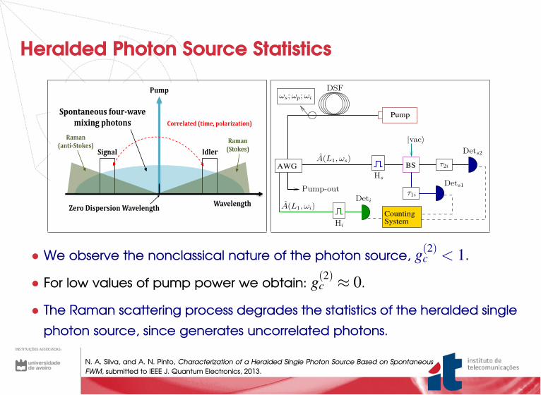
Heralded Photon Source Statistics

Pump

Idler Signal

Correlated (time, polarization)

Wavelength

Spontaneous four-wave mixing photons

Zero Dispersion Wavelength

Raman (anti-Stokes)

Raman (Stokes)

AWG BS

CountingSystem

Pump

Hs

A(L1, ωi)

|vac〉

Deti

Hi

DSF

Pump-out

τ2i

Dets1

Dets2

τ1i

ωs;ωp;ωi

A(L1, ωs)

• We observe the nonclassical nature of the photon source, g(2)c < 1.

• For low values of pump power we obtain: g(2)c ≈ 0.

• The Raman scattering process degrades the statistics of the heralded single

photon source, since generates uncorrelated photons.

N. A. Silva, and A. N. Pinto, Characterization of a Heralded Single Photon Source Based on Spontaneous

FWM, submitted to IEEE J. Quantum Electronics, 2013.

Entangled Photon Pairs Generation

In response to Einstein et al.’s paper, Niels Bohr answeredwith a paper of his own in which he states that the problemdoes not rely in the theory but in the way how measure-ments are performed, or more importantly, in the ways oneanalyzes a given phenomenon, focusing on the influence thatexperimental setups had over these measurements. With this,he introduced the concept of complementarity [5]. To furthersupport his view, later were presented a series of examplesbased on the wave-particle duality of matter [6–8].

B. Bell Theory

Following the work of John von Neumann[9] and DavidBohm [10, 11], John S. Bell devised a theory based on localhidden variables. In his paper, he presented a theorem basedon nonlocality terms, while the locality theory is based on twoassumptions [12]:

1) All objects have to be in a definite state from which thevalues of all other physical quantities can be determined,such as the position or momentum of an object.

2) The effects of local actions, such as measurements,cannot travel faster than the speed of light (as a resultof special relativity). If the observers are sufficiently farapart, the measurement made by one will have no effecton the one done by the other (and vice-versa).

Considering the correlation between measurements, thecausality condition imposed by local realism is upheld if theBell theorem is proved correct. Item 1) addresses the issueof locality, while item 2) issues the separability criterion. TheBell theorem is stated as the following [12, 13],

E(a, b) =

∫

λ∈Λ

p(λ)A(a, λ)B(b, λ)dλ , (2)

where Λ is the probability space, λ are the hidden variables,with A and B being two physical quantities, while a and bare the axis at which A and B are projected over.

In order to test the quality of the entangled states, it can bemeasured the CHSH inequality, which is one type of the Bellinequalities. From (2), the polarization correlation coefficient,which requires four correlation measurements, can be definedas follows [14]:

E(θ1, θ2) =Cθ1,θ2 + Cθ′1,θ′2 − Cθ1,θ′2 − Cθ′1,θ2Cθ1,θ2 + Cθ′1,θ′2 + Cθ1,θ′2 + Cθ′1,θ2

. (3)

In (3), Cθ1,θ2 are the coincidences between the polarizer ofAlice set at angle θ1 and the polarizer of Bob set at angle θ2,being θ′1 = θ1 + 90 and θ′2 = θ2 + 90. In the CHSH inequality,the parameter S is defined as [14]:

S = |E(θ1, θ2)− E(θ1, θ′2) + E(θ′1, θ2) + E(θ′1, θ

′2)| , (4)

and requires sixteen measurements. From quantum mechanics,the expectancy values for the CHSH inequality are,

E(θ1, θ2) = E(θ′1, θ2) = E(θ′1, θ′2) =

1√2, (5)

and,E(θ1, θ

′2) = − 1√

2. (6)

These are the maximum values, and lead also to the maximumvalue of S=2

√2. This value can be obtained when polariza-

tion angles are set to (θ1, θ′1, θ2, θ′2) = (0◦, 45◦, 22.5◦, 67.5◦).The uncertainty of the quantity S is given by,

σS =

√√√√16∑

i=1

Ci

(∂S

∂Ci

)2

, (7)

where the uncertainty of the ith measurement, Ci, isσCi

=√Ci [15].

To determine the existence of correlation between measure-ments, we estimate the values of each term in (4). If the sumis greater than 2, the Bell inequality is violated and this leadsto physical reality being nonlocal, hence existing correlationbetween measurements. If not, local realism prevails and thereis no correlation at all. Besides this, there are other limits andassumptions that need to be verified, regarding visibility andeffective quantum efficiency values, among others. Consider-ing quantum mechanics, there is also a maximum limit ofcorrelation [16–18].

III. EXPERIMENTAL SETUP

In order to verify the effectiveness of our method of genera-tion of polarization-entangled photon pairs, we used the setuppresented in Fig. 1. A pump from a tunable laser source (TLS),with a full width at half maximum of 830 ps and a repetitionrate of 2.2 MHz passes through an optical circulator, and afiber Bragg grating (FBG), in order to eliminate the sidebands.The TLS is centered at 1550.918 nm wavelength, which isat the zero-dispersion wavelength of the HNLF used in theexperiment. At the output of the optical circulator, the photons’polarization should be adjusted using a polarization controller(PC1), so that when they are focused in the Mach-Zehnder(MZ) modulator’s LiNbO3 crystal has maximum efficiency.The MZ modulator is connected to a DC voltage source anda pattern generator. At the output of the MZ modulator isan erbium doped fiber amplifier (EDFA), which is used toamplify the pump’s optical power. The noise from the EDFA iseliminated using a 100 GHz flat fixed optical filter. In order tomatch the 45◦ port of the polarization beam splitter (PBS), the

Pump (TLS)1550.918 nm

HNLF

PC2 LP

Pattern generator

MZ modulator

FBG

Isolator

APD2

DC Voltage

PC4

PC

3

450

900

00

3

1

24

AWGFi

Fs

APD1

RLP2

EDFA

HWP2

RLP1 HWP1

QWP2

QWP1

PC1

isis

VVHH 2

1

Filter

Filter

Time TaggingModule

1

2

Signal

Idler

PBS

Fig. 1. Experimental scheme used for polarization-entangled photon pairgeneration through spontaneous four-wave mixing and coincidence detection.

N. A. Silva, and A. N Pinto, Role of Absorption on the Generation of Quantum-Correlated Photon Pairs

Through FWM, IEEE Journal of Quantum Electronics, Vol. 48, No. 11, pp. 1380-1388, 2012.

Code, Transmit and Recovery Information• The QBER can be calculated as

QBER = [wrong counts]/[total counts]

PC1

PC6

PC5

PumpPulse

λ=1550.92nmMZ

Modulator

LP4

APD2

APD1

Microcontroller

PC

Trigger

LP3

AOM2

|V>,bit1

|H>,bit0

CH2

CH1

id200

id201

AOM1

Fiber

50:50

50:50

PC4

PC3

TTL

TTL

DATA

Trigger

VOA

5:95

SyncPulse

λ=1563.05nm

AWGPIN

DC

Pattern

Generator

PC2

DATA

LP2

LP1

|H>,bit0

|V>,bit1

CH2

CH1

50:50

Filter

Filter

Experimental arrangement

0 . 0 1 . 5 3 . 0 4 . 5 6 . 0 7 . 5 9 . 0 1 0 . 5 1 2 . 00

1 0

2 0

3 0

4 0

5 0

QBER

(%)

T i m e ( H o u r s )

B a c k - t o - B a c k L = 2 0 k m

Experimental measurements

• The QBER presents a random evolution with time, due to the SOP drift.

A. J. Almeida, J.M. Prata, N. J. Muga, N. A. Silva, P. S. André, A.N. Pinto, Continuous Control of

Random Polarization Rotations for Quantum Communications, IEEE/OSA J. of Lightwave Technology, 2016

(accepted for publication).

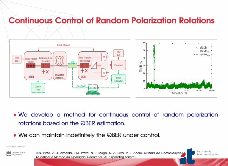
Continuous Control of Random Polarization Rotations

Processor

D2

D1

EPC Single-Photon

Source

QUANTUM CHANNEL

ALICE BOB

Algorithm

Basis Selection (Encoding)

Basis Selection (Decoding)

Feedback

Data Bits

QBER Estimator

Raw Key

Control Bits

PBS

Public Channel

For Review Only

JOURNAL OF LIGHTWAVE TECHNOLOGY 7

MZMPC-1Signal

OS-1

VOA

SPAD-1

SPAD-2

PBS-1

PC-3

PC-2Pulse Pattern

Generator

EPC

ComputerFeedback

OpticalFiber

Quantum Channel

ALICE

BOB

HWP

PBS-2 PIN

Computer

Sync. Laser

OS-2

Fig. 6. Scheme of the experimental setup for the proof-of-principle demon-stration of the method.

and SPAD-2). The two detectors are InGaAs/InP avalanchephotodiodes operating in a gated Geiger mode. Detector 1(id200) has a dark count probability per time gate tg = 5 nsof Pdc =4.47×10−4 ns−1 and a quantum detection efficiencyηD≈10 %. Detector 2 (id201) has a dark count probability pertime gate tg = 5 ns of Pdc = 2.07×10−4 ns−1 and a quantumdetection efficiency ηD ≈ 10 %. In order to compensate forrandom rotations of polarization in the optical fiber, we use anEPC (PolaRITETM II/III from General Photonics) consistingof four piezoelectric squeezers running voltages up to about150 V (V1...4). Each squeezer has two possible changes forits voltage, V1...4±, ‘+’ for increase and ‘-’ for decrease. TheQBER of the measurement is estimated and then used as afeedback parameter for the control algorithm, which will actin the EPC. To perform synchronization between Alice andBob, a laser set at λs = 1547.72 nm is used. After the laserwe use another optical switch (OS-2) working at the samerepetition rate of the signal (100 kHz), which is received by aclassical detector (PIN) that gives trigger to detectors SPAD-1and SPAD-2. In this way, the detectors will be ready to openthe gate only when a single photon is expected.

B. Experimental Results

In the implementation of the experimental setup of Fig. 6,Alice transmitted frames with size FS = 217 bits. To verifyif the method to compensate random rotations of polarizationcould work in practice, we have used a 40 km optical fiber as atransmission channel between Alice and Bob. The system wasinitially adjusted to give the lowest error rate and then started.After some time, an external perturbation was applied, byrotating the waveplate before the fiber. A plot of the evolutionof the QBER with time can be seen in Fig. 7. Results show thatthe system is able to work at a low QBER for several hours,most of the time below QBERMax. It is also worth noting that,

0 0 : 0 0 0 1 : 0 0 0 2 : 0 0 0 3 : 0 0 0 4 : 0 0 0 5 : 0 00

1 0

2 0

3 0

4 0

5 0

6 0

T i m e [ h o u r s ]

QB

ER [%

]

Q B E R Q B E R M i n Q B E R M a x

Fig. 7. Experimental results on the evolution of the QBER with time,including an external perturbation after about 30 minutes running. Thequantum channel used was a 40 km optical fiber. The theoretical limits weredefined as: QBERMin = 2% and QBERMax = 11%.

after applying an external perturbation to the system (aroundthe minute 30), the polarization control method was able torecover the QBER to the initial value and continue to work ina stable way. The average QBER during the 5-hour running,whenever QBER ≤ QBERMax, was 3.2 %. Regarding Ns, wehave obtained an average value of 12.5 % per frame. Fromthe experimental results obtained we are able to concludethat the polarization control method is robust and effective tocompensate the perturbations in the system and that an averagebandwidth of 87.5 % is able to be used in the transmission ofdata qubits, in average.

VII. CONCLUSIONS

We have presented a method to compensate random ro-tations of polarization in quantum communication systems,which is based on an accurate estimation of the QBER. Themethod allows the automatic control of polarization withoutinterruption in data transmission. In the proposed schemewere used frames containing control and data qubits, bothobtained from quantum signals. A theoretical model for theestimation of the QBER was derived from the Clopper-Pearsonconfidence interval. It was demonstrated that this methodallows to control polarization even when long fiber links areused as a quantum channel. A polarization control algorithmwas described and successfully verified through numericalsimulations and experimental measurements. These resultshave shown that the method is practical, efficient and robustto large perturbations in the fiber. At last, we have presentedan experimental validation of the method in a long run, usingan optical fiber with 40 km as a quantum channel. Effectivecontrol of polarization was observed, showing an average errorrate of 3.2 %, while consuming 12.5 % of the frame size, inaverage, with control qubits.

REFERENCES

[1] N. Gisin, G. Ribordy, W. Tittel, and H. Zbinden, “Quantum cryptogra-phy,” Rev. Mod. Phys., vol. 74, pp. 145–195, Jan. 2002.

Page 7 of 8 Journal of Lightwave Technology

123456789101112131415161718192021222324252627282930313233343536373839404142434445464748495051525354555657585960

• We develop a method for continuous control of random polarization

rotations based on the QBER estimation.

• We can maintain indefinitely the QBER under control.

A.N. Pinto, A. J. Almeida, J.M. Prata, N. J. Muga, N. A. Silva, P. S. André, Sistema de Comunicações

Quânticas e Método de Operação, December, 2015 (pending patent).

Quantum Key Distribution - BB84 Protocol

9

17

QKD Development QKD Development -- SystemsSystems

18

Cerberis SolutionCerberis Solution

• The presence of Eve increases the QBER.

• Monitoring the QBER the presence of Eve can be detected.

• For a QBER < 17.5% is possible to process the exchanged information to

make sure that Eve cannot obtain any valuable information from the keys.

ID Quantique - Cerberis Solution.

In Summary• We are using a very small number of photons per symbol, to increase the capacity

and functionalities of fiber-optic communication systems.

• We are able to prepare several quantum photon states.

• We are able to code information in the photons polarization.

• We are able to transmit the quantum states through standard single mode fibers.

• The random polarization drift degrades severely the system performance.

• We are able to actively compensate for random polarization rotations maintaining

a low QBER value.

• We are implementing quantum protocols which allows to solve trust issues in many

real-world applications (ongoing work).

E-mail: anp@ua.pt