P t 3Part 3Chapter 9Chapter 9

G Eli i tiGauss Elimination

All images copyright © The McGraw-Hill Companies, Inc. Permission required for reproduction or display.

PowerPoints organized by Dr. Michael R. Gustafson II, Duke UniversityRevised by Prof. Jang, CAU

Chapter ObjectivesChapter ObjectivesKno ing ho to sol e small sets of linear eq ations• Knowing how to solve small sets of linear equations with the graphical method and Cramer’s rule.

• Understanding how to implement forward elimination g pand back substitution as in Gauss elimination.

• Understanding how to count flops to evaluate the efficiency of an algorithmefficiency of an algorithm.

• Understanding the concepts of singularity and ill-condition.

d di h i l i i i i l d• Understanding how partial pivoting is implemented and how it differs from complete pivoting.

• Recognizing how the banded structure of a tridiagonalRecognizing how the banded structure of a tridiagonalsystem can be exploited to obtain extremely efficient solutions.

Graphical MethodGraphical Method• Small numbers (n<=3) of

equations: Graphical methodequations: Graphical method, Cramer’s rule, elimination of unknowns.

• For small sets of simultaneous equations, graphing them and determining the location ofdetermining the location of the intercept provides a solution.

• Ex. for three (two) simultaneous equations, the point where the three planespoint where the three planes (two lines) intersect would represent the solution.p

Graphical Method (cont)p ( )• Graphing the equations can also show

systems where:systems where:a) No solution existsb) Infinite solutions exist

Singularb) Infinite solutions existc) System is ill-conditioned

• Extremely sensitive to roundoff errorAlmost Singular

Extremely sensitive to roundoff error.• The point of intersection is difficult to detect

visually.

DeterminantsDeterminants• The determinant D=|A| of a matrix is formed from theThe determinant D |A| of a matrix is formed from the

coefficients of [A].• Determinants for small matrices are:

11 a11 a11

a11 a122 2a11 a12

a21 a22

a11a22 a12a21

a11 a12 a13

3 3a11 a12 a13

a21 a22 a23

a a a a11

a22 a23

a32 a33

a12

a21 a23

a31 a33

a13

a21 a22

a31 a32

• Determinants for matrices larger than 3 x 3 can be very

a31 a32 a33

complicated.

Cramer’s RuleCramer s Rule

• Cramer’s Rule states that each unknown in a system of linear algebraic equations y g qmay be expressed as a fraction of two determinants with denominator D anddeterminants with denominator D and with the numerator obtained from D by replacing the column of coefficients ofreplacing the column of coefficients of the unknown in question by the constants b1, b2, …, bn.

Cramer’s Rule ExampleCramer s Rule Example

i d i h f ll i f i• Find x2 in the following system of equations:0.3x1 0.52x2 x3 0.01

0.5x1 x2 1.9x3 0.67

• Find the determinant D0.1x1 0.3x2 0.5x3 0.44

0.3 0.52 11 1.9 0.5 1.9 0.5 1

• Find determinant D by replacing D’s second column with b

D 0.5 1 1.90.1 0.3 0.5

0.3.9

0.3 0.5 0.52

0.5 .90.1 0.5

10.50.1 0.4

0.0022

• Find determinant D2 by replacing D s second column with b

D2 0.3 0.01 10.5 0.67 1.9 0.3

0.67 1.90 44 0

0.010.5 1.90 1 0

10.5 0.670 1 0 44

0.0649

• Divide

2

0.1 0.44 0.50.44 0.5 0.1 0.5 0.1 0.44

D 0 0649x2 D2

D

0.06490.0022

29.5

Naïve Gauss EliminationNaïve Gauss Elimination

F l t C ’ R l• For larger systems, Cramer’s Rule can become unwieldy.

• Instead a sequential process of removing• Instead, a sequential process of removing unknowns from equations using forward elimination followed by backwardelimination followed by backward substitution may be used - this is Gauss elimination.

• “Naïve” Gauss elimination simply means the process does not check for potential

bl l i f di i i bproblems resulting from division by zero. ->not need pivoting.

Naïve Gauss Elimination (cont)( )

• Forward elimination– Starting with the first row, add or

subtract multiples of that row to eliminate the first coefficient from the second row and beyond.y

– Continue this process with the second row to remove the second coefficient from the third row and beyondbeyond.

– Stop when an upper triangular matrixremains.

• Back substitution– Starting with the last row, solve for

the unknown, then substitute that l i t th t hi h tvalue into the next highest row.

– Because of the upper-triangular nature of the matrix, each row will contain only one more unknown.y

Naïve Gauss Elimination (cont)

• N equations:

( )

N equations:

Pi t l t Pi t ti

n bxaxaxaxa 111113112111

Pivot element Pivot equation

n bxaxaxaxa

222223222121

nnnnnnn bxaxaxaxa 332211

Naïve Gauss Elimination (cont)

Forward Elimination:

( )

Forward Elimination: Reduce the set of equations to an upper triangular

matrix.

Eliminate the first unknown x1 from the second through the nth equations. To do this, multiply the first equation by a21/a11to givegive

111

211

11

21313

11

21212

11

21121 b

aaxa

aaxa

aaxa

aaxa nn

This equation can be subtracted from the second equation by:

aaa

111

2121

11

212212

11

2122 b

aabxa

aaaxa

aaa nnn

''' b22222or bxaxa nn

Naïve Gauss Elimination (cont)The procedure is repeated for the remaining equations.

( )

''''

'2

'23

'232

'22

11313212111

nn

nn

bxaxaxabxaxaxabxaxaxaxa

''3

'32

'2

33333232

nnnnnn

nn

bxaxaxa

bxaxaxa

Using the second pivot equation to remove x2 from the third through the nth equations to give

3322 nnnnnn

through the nth equations to give

'2

'23

'232

'22

11313212111

nn

nn

bxaxaxabxaxaxaxa

"""

"3

"33

"33

22323222

nn

nn

bxaxa

""3

"3 nnnnn bxaxa

Naïve Gauss Elimination (cont)

l h h f ll i f i

( )

Lastly we can have the following set of equations:

11313212111 nn bxaxaxaxa

"3

"33

"33

'2

'23

'232

'22

nn

nn

bxaxabxaxaxa

)1()1( nnn

nnn bxa

Naïve Gauss Elimination (cont)

Backward substitution

( )

ac a d subst tut o

'2

'23

'232

'22

11313212111

nn

nn

bxaxaxabxaxaxaxa

"3

"33

"33

22323222

nn

nn

bxaxa

)1()1( nnn

nnn bxa

)1( nb 1

)1()1( n

ijj

iij

ii xab

(i 1 2 1)

)1( nnn

nn a

bx)1(1

iii

iji a

x

There is only one variable (i = n-1, n-2, ,1)There is only one variable in the (n-1)th row.

Example 9 3 (1/2)Example 9.3 (1/2)Q. Use the Gaussian elimination to find the solution.

(S l ti 3 2 5 d 7)(Solution: x1 = 3, x2 = -2.5, and x3 = 7)

3193071085.7 0.21.03 321

xxxxxx

Forward elimination:

4.71 10 .203.03.193.07 1.0

321

321

xxxxxx

Forward elimination:

5617.19293333.07.00333 85.7 0.2 1.0 3

32

321

xxxxx

6150.70 0200.10 190000.0 32 xx

8570 2103 xxx

0843.70 0120.10 5617.19293333.07.00333 85.70.2 1.0 3

3

32

321

xxxxxx

3

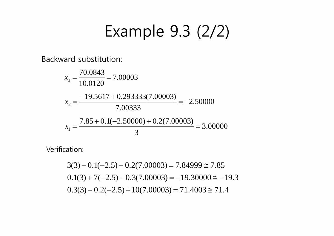
Example 9.3 (2/2)p ( / )

Backward substitution:

결과를 확인하면 00003.70120.100843.70

3 x

50000.200333.7

)00003.7(293333.05617.192

x

00000.33

)00003.7(2.0)50000.2(1.085.71

x

85.784999.7)00003.7(2.0)5.2(1.0)3(3

Verification:

4.714003.71)00003.7(10)5.2(2.0)3(3.03.1930000.19)00003.7(3.0)5.2(7)3(1.0

Naïve Gauss Elimination ProgramNaïve Gauss Elimination Program

Gauss Program EfficiencyGauss Program Efficiency• The execution of Gauss elimination depends on theThe execution of Gauss elimination depends on the

amount of floating-point operations (or flops). The flop count for an n x n system is:

ForwardElimination

2n3

3O n2 3

BackSubstitution n2 O n

2 3

Total 2n3

3O n2

• Conclusions:– As the system gets larger, the computation time increases greatly.

f h ff i i d i h li i i– Most of the effort is incurred in the elimination step.

PivotingPivoting

P bl i ith ï G li i ti if• Problems arise with naïve Gauss elimination if a coefficient along the diagonal is 0 (problem: division by 0) or close to 0 (problem: round-off y ) (perror)

• One way to combat these issues is to determine the coefficient with the largest absolute value inthe coefficient with the largest absolute value in the column below the pivot element. The rows can then be switched so that the largest element i h i l Thi i ll d i l i iis the pivot element. This is called partial pivoting.

• If the rows to the right of the pivot element are also checked and columns switched this is calledalso checked and columns switched, this is called complete pivoting. -> It is rarely used. Add complexity.

Partial Pivoting Programg g

Example 9 4 ( ti l i ti ) (1/3)Example 9.4 (partial pivoting) (1/3)Q. Use the Gaussian elimination to solve this.

0001.20000.30003.0 21 xx

0 0003 i l t 0 ti l i ti i

0000.10000.10000.1 21 xx

a11 = 0.0003 is very close to 0, so partial pivoting is made. Solution: x1 = 1/3 and x2 = 2/3Solution: x1 = 1/3 and x2 = 2/3.

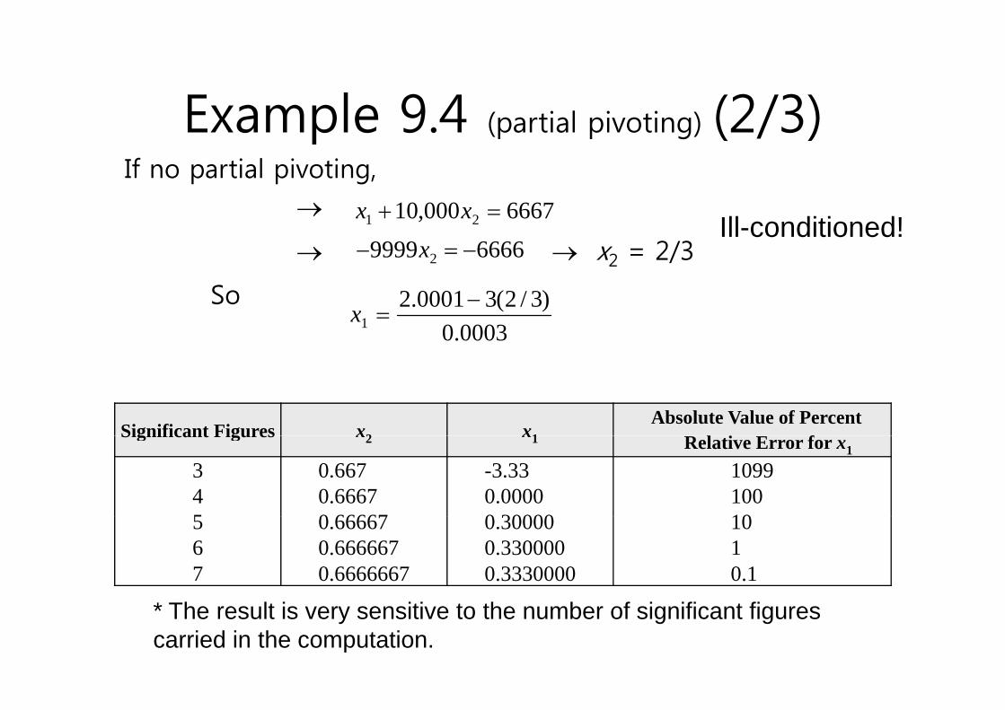
Example 9 4 ( ti l i ti ) (2/3)If no partial pivoting,

Example 9.4 (partial pivoting) (2/3)

x2 = 2/3

6667000,10 21 xx66669999 2 x

Ill-conditioned!

So0003.0

)3/2(30001.21

x

Significant Figures x2 x1Absolute Value of Percent

Significant Figures x2 x1 Relative Error for x1

345

0.6670.66670 66667

-3.330.00000 30000

1099100105

67

0.666670.6666670.6666667

0.300000.3300000.3330000

1010.1

* The result is very sensitive to the number of significant figures carried in the computation.

Example 9.4 (partial pivoting) (3/3)p (p p g) ( / )• With partial pivoting

x2 = 2/3 and0000.10000.10000.1 21 xx0001.20000.30003.0 21 xx

)3/2(1x

Significant Figures x2 x1Absolute Value of Percent

11 x

Significant Figures x2 x1 Relative Error for x1

345

0.6670.66670 66667

0.3330.33330 33333

0.10.010 0015

67

0.666670.6666670.6666667

0.333330.3333330.3333333

0.0010.00010.00001

Tridiagonal SystemsTridiagonal Systems• A tridiagonal system is a banded system with aA tridiagonal system is a banded system with a

bandwidth of 3:f1 g1

x1 r1 f1 g1e2 f2 g2

e3 f3 g3

x1x2x3

r1r2r3

e f g

x 1

r 1

• Tridiagonal systems can be solved using the same

en1 fn1 gn1en fn

xn1xn

rn1

rn

• Tridiagonal systems can be solved using the same method as Gauss elimination, but with much less effort because most of the matrix elements areeffort because most of the matrix elements are already 0.

Tridiagonal System SolverTridiagonal System Solver