Policy Space in Agricultural Markets -...

U n i t e d n at i o n s C o n f e r e n C e o n t r a d e a n d d e v e l o p m e n t

POLICY SPACE IN AGRICULTURAL MARKETS

POLICY ISSUES IN INTERNATIONAL TRADE AND COMMODITIESRESEARCH STUDY SERIES No. 73

Printed at United Nations, Geneva1600845 (E) – January 2016 – 245

UNCTAD/ITCD/TAB/75

United Nations publicationISSN 1607-8291

POLICY ISSUES IN INTERNATIONAL TRADE AND COMMODITIES

RESEARCH STUDY SERIES No. 73


by

Alain McLaren

UNCTAD, Geneva

New York and Geneva, 2016

U N I T E D N AT I O N S C O N F E R E N C E O N T R A D E A N D D E V E L O P M E N T

ii POLICY ISSUES IN INTERNATIONAL TRADE AND COMMODITIES

Note

The purpose of studies under the Research Study Series is to analyse policy issues and to

stimulate discussions in the area of international trade and development. The Series includes

studies by UNCTAD staff and by distinguished researchers from other organizations and academia.

The opinions expressed in this research study are those of the authors and are not to be

taken as the official views of the UNCTAD secretariat or its member States. The studies published

under the Research Study Series are read anonymously by at least one referee. Comments by

referees are taken into account before the publication of studies.

The designations employed and the presentation of the material do not imply the

expression of any opinion on the part of the United Nations concerning the legal status of any

country, territory, city or area, or of authorities or concerning the delimitation of its frontiers or

boundaries.

Comments on this paper are invited and may be addressed to the author, c/o the

Publications Assistant, Trade Analysis Branch (TAB), Division on International Trade in Goods and

Services, and Commodities (DITC), United Nations Conference on Trade and Development

(UNCTAD), Palais des Nations, CH-1211 Geneva 10, Switzerland; e-mail: [email protected]; fax no:

+41 22 917 0044. Copies of studies under the Research Study Series may also be obtained from

this address.

Studies under the Research Study Series are available on the UNCTAD website at

http://unctad.org/tab.

Series Editor:

Chief Trade Analysis Branch

DITC/UNCTAD

UNCTAD/ITCD/TAB/75

UNITED NATIONS PUBLICATION

ISSN 1607-8291

© Copyright United Nations 2016 All rights reserved

Policy Space in Agricultural Markets iii

Abstract

As an outcome of the Uruguay Round Agreement on Agriculture, all agricultural products now have a

bound tariff rate on their imports. This system of bound tariffs combines the rigidity of an upper limit

that is independent of future economic conditions but discretion as governments have a whole array of

choices in terms of applied tariffs as long as they are set below the bound rate. One recurring

argument is that bound rates may limit countries’ policy flexibility, or policy space, in response to

particular economic circumstances. This paper looks at the use and availability of this policy space in

agricultural markets. This is first done in a descriptive setting, then by assessing what plays a role in

determining this space using an empirical analysis. A general finding is that policy space in agricultural

products is generally available, and only limited for developed countries. Many developing countries

have ample room to raise tariffs in most agricultural imports without infringing binding commitments.

For LDCs there is virtually no imports for which policy space is not available. The findings indicate that

four specific factors are related to the use of policy space, which are the elasticity of import demand,

the fact that the goods are being used as intermediates, food security and protection of local

producers. The results suggest that policy space tends to be used relatively less for products with

lower elasticity of demand and for intermediate products. In regard of products relevant for food

security, the results suggest that policy space is larger. In regard to products that face domestic

competitors, the results indicate lower tariff water and more use of policy space, suggesting that

producer protection is an issue related to the level of policy space to use and the level of market

protection to set.

Keywords: International trade, policy space, WTO, tariffs.

JEL Classification: F10, F13

iv POLICY ISSUES IN INTERNATIONAL TRADE AND COMMODITIES

Acknowledgements

This study was prepared during my stay in the Trade Analysis Branch under the Division for International Trade and Commodities at UNCTAD. The author wishes to thank Marco Fugazza,

Alessandro Nicita, and Ralf Peters for discussion and comments. This paper represents the personal views of the author only, and not the views of the UNCTAD

secretariat or its member States. The author accepts sole responsibility for any errors remaining.

Policy Space in Agricultural Markets v

Contents

1 INTRODUCTION .......................................................................................................................... 1

2 DATA ........................................................................................................................................... 2

3 POLICY SPACE ........................................................................................................................... 3

4 EMPIRICAL SPECIFICATION ................................................................................................... 10

5 ROBUSTNESS CHECKS ........................................................................................................... 15

6 CONCLUSION ........................................................................................................................... 17

BIBLIOGRAPHY ...................................................................................................................................... 18

vi POLICY ISSUES IN INTERNATIONAL TRADE AND COMMODITIES

List of figures

Figure 1. Policy space and the share of trade covered ........................................................................ 4

Figure 2. Policy space and gross domestic product per capita ........................................................... 5

Figure 3. Policy space in least developed countries, at the HS 2 digit level ........................................ 6

Figure 4. Policy space in developing non-LDCs, at the HS 2 digit level .............................................. 7

Figure 5. Share of imports from partners within RTAs, by income level .............................................. 8

Figure 6. Policy space .......................................................................................................................... 9

Figure 7. Policy space for imported and produced goods ................................................................... 9

List of tables

Table 1. OLS and fractional heteroskedastic probit .......................................................................... 12

Table 2. Water and true water by income group (OLS) ..................................................................... 13

Table 3. MFN/bound and true MFN/bound by income group (OLS) ................................................. 14

Table 4. MFN/bound and true MFN/bound by income group (Fract. Heter. Probit) ......................... 14

Table 5. OLS and fractional heteroskedastic probit at the HS 6 digit level ...................................... 15

Table 6. OLS and fractional heteroskedastic probit excluding the import demand elasticity .......... 16

Policy Space in Agricultural Markets 1

1. INTRODUCTION

Trade in agri-food products is governed by a set of rules influencing market access conditions by

limiting the level of protection countries can legitimately apply. At the multilateral level, the rules

governing the trade of agricultural products are those agreed in the Uruguay Round Agreement on

Agriculture (URAA). The URAA was concluded in 1994 and became fully implemented by 2005. As an

outcome of the URAA each WTO member replaced border barriers with an equivalent tariff. This tariff is

known as the "bound rate" and refers to the highest rate the country could then apply without infringing

the agreement.1 The rationale behind setting tariff ceilings was to increase policy certainty and limit

negative spillovers of domestic policies on international markets. As noted in Horn et al. (2010), the

system of bound tariffs combines the rigidity of an upper limit that is independent of future economic

conditions but discretion as governments have a whole array of choices in terms of applied tariffs as

long as it stays below the bound rate. Still, one recurring argument is that bound rates may limit

countries’ policy flexibility (or policy space) in response to particular economic circumstances.

In reality, countries often choose to apply a tariff that is well below the bound rate, and thus generally

maintain significant flexibility in raising the tariffs of many agricultural products. This flexibility can be

measured by the difference between the bound and the “most favoured nation” tariff rate (MFN) and is

referred to as tariff water or binding overhang. In order to understand the use that developing countries

do, or don't do, of such flexibility, this paper examines the availability and use of policy space related to

agricultural trade.2

There are a certain number of reasons for which the desired MFN is often set below the bound rate and

thus policy space remains available. Theoretical work by Amador and Bagwell (2012) considers that

governments set tariffs so as to maximize a weighted average of consumer surplus, tariff revenue and

profits in the import-competing sector. They will be influenced by many economic factors, some of

which will affect several of them simultaneously. This paper investigates some of the most relevant

factors that can influence the use of policy space. In particular, the paper examines the relationship

between policy space and the elasticity of import demand, the fact that the goods are being used as

intermediates, food security and protection of local producers.

The elasticity of import demand will have a direct impact on consumer surplus and will influence the

amount of tariff revenue through changes in import volumes. For example, if a government's objective

is to reduce demand of imports, small changes in tariffs on products with elastic demand would be

rather effective, while any raise in tariff would not substantially impact imports of products with inelastic

demand which lack of domestic substitutes. In contrast, tariff setting would be quite different if the

government’s objective is to increase tariff revenues. In practice, governments under fiscal constraints

may be willing to use their policy space on products with inelastic demand. The use of policy space

may also be related to whether the good is used as an intermediate product. In such cases

policymakers may be inclined to keep the MFN applied relatively low thus favoring local processing

1 The guidelines were the following for developed countries, as found in Multilateral Trade Negotiations on Agriculture (2000): for previously bound tariff lines, they had to keep on using the same rate if there was no NTB, and if there was an

NTB they had to eliminate it or use the following tariffication formula: T = �� ∗ 100.For lines that were not previously

bound, they had to use the rate that was applied as of September 1986 if there was no NTB, and if there was an NTB they had to use the tariffication formula. For developing countries, the guidelines were the same for lines that were already bound. For those that were not previously bound, they had the choice to do as developed countries or offer a ceiling binding.

2 The present study does not look at whether the bound rate has a useful purpose when it is well above the applied rate. The literature tends to agree on the fact that the bound rate may nonetheless play a positive role for several reasons. For instance, Bacchetta and Piermartini (2011) note that this situation implies increased tariff stability as well as reduced uncertainty that exporters face in terms of trade policy. They also mention that theoretical work by Francois and Martin (2004) showed that there are welfare gains from both the reduced variability of tariffs and their lower average level. Bacchetta and Piermartini (2011) also put forward the argument found in Sala et al. (2010), who argue that a bound rate above the applied rate may not directly affect the intensive margin that will be influenced by the applied rate but may give a signal to exporters wishing to enter that there is more stability on the market. This was confirmed empirically in Handley (2014).

2 POLICY ISSUES IN INTERNATIONAL TRADE AND COMMODITIES

industries. However, it is possible that government strategies aimed to integrate vertical production

processes use all their policy space so as to facilitate the emergence of domestic suppliers.3 A third

factor affecting the use of policy space is food security. In this regard, the main argument is to support

local production so as to guarantee food supply from domestic producers while minimizing the effect of

external shocks. However, countries with insufficient agricultural resources rely more on food supply

from international markets and therefore may be seeking food security by facilitating trade on foodstuff

thus making little use of any available policy space. Finally, a reason for which one may expect

governments to set higher applied tariffs could be related to the presence of producers’ lobbies which

influence government decisions related to trade policy. If there aren't any domestic producers then

there won't necessarily be an incentive to increase the price of the imported product.

In investigating the use of policy space this paper will first show some descriptive statistics of policy

space in agriculture, by using a snapshot of recent data, namely 2013. It shows the distribution of

policy space with respect to trade covered, the relationship between policy space and GDP per capita,

and finally the distribution of policy space by product and by income level groups. A first finding

indicates that in the vast majority of cases policy space is available, meaning that countries could raise

tariffs if they wanted to. The second step is to perform econometric analysis to shed light on what

determines policy space. This is done over a longer time span in order to benefit from the advantages

of panel data techniques. The results suggest that the elasticity of import demand, intermediate goods,

food security issues and protection of local producers are all correlated to the amount of policy space

that is available. The information on what plays a strong role in influencing policy space and in which

way can have important policy implications, especially in present times where negotiations on new

bound rates are having trouble reaching consensus, and in particular in agriculture which has also been

one of the tough areas in terms of trade policy negotiations.

The rest of the paper is organized as follows. Section 2 presents the data that will be used for the

descriptive statistics and regressions, section 3 shows and discusses some stylized facts concerning

policy space, section 4 presents the empirical specifications used, section 5 presents some robustness

checks and section 6 concludes.

2. DATA

The tariff data used comes from the UNCTAD TRAINS database and includes ad valorem equivalents

using the UNCTAD method 1. It includes bound rates and MFN applied rates as an import value

weighted average at the HS 6 digit level. The import data comes from the UN COMTRADE database,

food production data comes from the Food and Agricultural Organization (FAO) of the United Nations

and the elasticity of import demand from Kee et al. (2008). All data except for production covers the

period 2008-2013 at the HS 6 digit level, covering 98 importing countries. The production data stops in

2012 and is converted from the FAO classification to an equivalent HS 2 digit level.

3 This relates to international trade and value chains, notably discussed in reports such as Humphrey and Memedovic

(2006) and in the Organisation for Economic Co-operation and Development's (OECD) Mapping Global Value Chains (2012).


3. POLICY SPACE

A first look at the data shows us that there is a reasonable amount of variation of policy space over

time, both increasing and decreasing. It is the changes in MFN applied that reflect the changes in

observed policy space.4 MFN applied tariff decreases were observed to be more frequent than tariff

increases, with about 9 percent of total lines (at the HS 6 digit level) that saw a decrease from one year

to the next against less than 6 percent that went up.5 However, the percentage of lines in the

agricultural data over the period 2008-2013 that increased and hit the bound was only of 0.2 percent of

all lines (and about 4 percent of increased tariffs), and just under 0.5 percent of all lines increased and

were over 80 percent of the bound after the increase (whether they already were above this threshold

or not). This shows us that although there is a reasonable amount of changes in the MFN applied rates,

both up and down, all of the available policy space is nearly never used up.

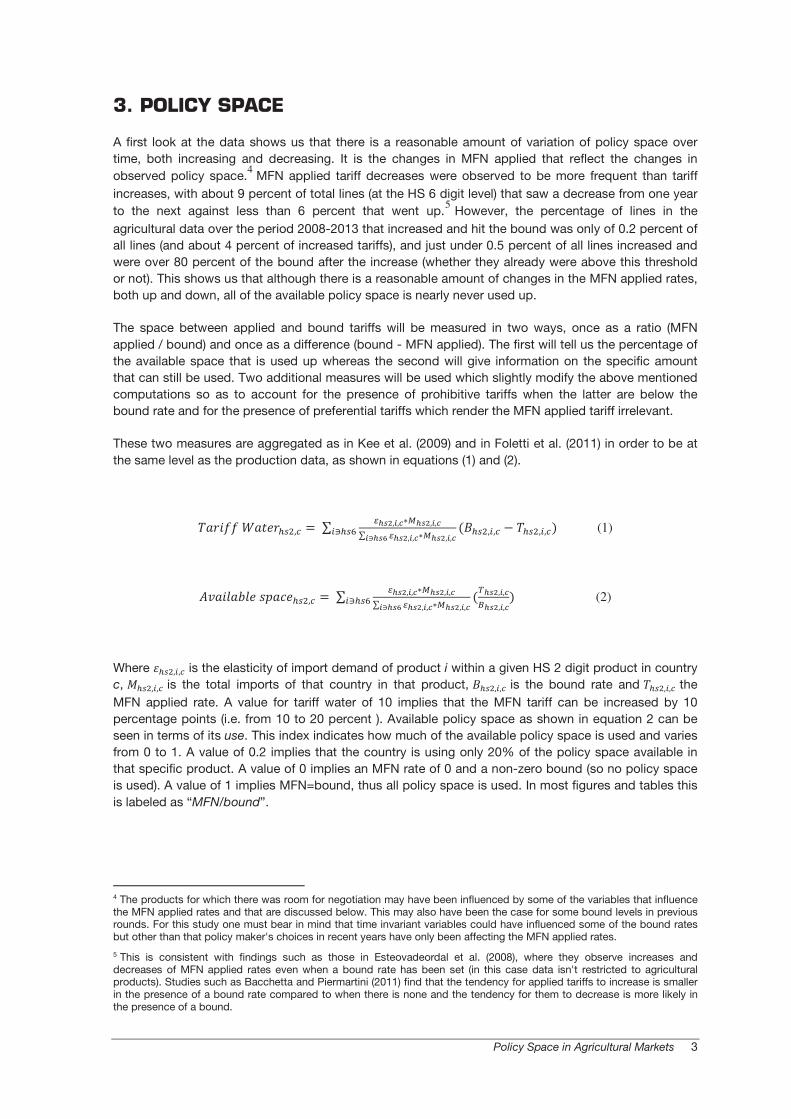
The space between applied and bound tariffs will be measured in two ways, once as a ratio (MFN

applied / bound) and once as a difference (bound - MFN applied). The first will tell us the percentage of

the available space that is used up whereas the second will give information on the specific amount

that can still be used. Two additional measures will be used which slightly modify the above mentioned

computations so as to account for the presence of prohibitive tariffs when the latter are below the

bound rate and for the presence of preferential tariffs which render the MFN applied tariff irrelevant.

These two measures are aggregated as in Kee et al. (2009) and in Foletti et al. (2011) in order to be at

the same level as the production data, as shown in equations (1) and (2).

� �� ,� =∑ ��,�,�∗ ��,�,�∑ ��,�,�∗ ��,�,��∋��" ($��,%,� − ��,%,�)%∋��( (1)

)* �+ ,+�-. /��,� =∑ ��,�,�∗ ��,�,�∑ ��,�,�∗ ��,�,��∋��" (0��,�,�1��,�,�)%∋��( (2)

Where 2��,%,� is the elasticity of import demand of product i within a given HS 2 digit product in country c, 3��,%,� is the total imports of that country in that product, $��,%,� is the bound rate and ��,%,� the MFN applied rate. A value for tariff water of 10 implies that the MFN tariff can be increased by 10

percentage points (i.e. from 10 to 20 percent ). Available policy space as shown in equation 2 can be

seen in terms of its use. This index indicates how much of the available policy space is used and varies

from 0 to 1. A value of 0.2 implies that the country is using only 20% of the policy space available in

that specific product. A value of 0 implies an MFN rate of 0 and a non-zero bound (so no policy space

is used). A value of 1 implies MFN=bound, thus all policy space is used. In most figures and tables this

is labeled as “MFN/bound”.

4 The products for which there was room for negotiation may have been influenced by some of the variables that influence the MFN applied rates and that are discussed below. This may also have been the case for some bound levels in previous rounds. For this study one must bear in mind that time invariant variables could have influenced some of the bound rates but other than that policy maker's choices in recent years have only been affecting the MFN applied rates.

5 This is consistent with findings such as those in Esteovadeordal et al. (2008), where they observe increases and decreases of MFN applied rates even when a bound rate has been set (in this case data isn't restricted to agricultural products). Studies such as Bacchetta and Piermartini (2011) find that the tendency for applied tariffs to increase is smaller in the presence of a bound rate compared to when there is none and the tendency for them to decrease is more likely in the presence of a bound.


0.2

.4.6

.81

0 50 100 150 200water

LDCs DevelopingDeveloped

Distribution of tariff water in termsof the value of trade

0.2

.4.6

.81

0 .2 .4 .6 .8 1pp


Distribution of mfn / bound in termsof the value of trade

Availability and use of policy space is different across countries depending on the level of

development.6 Figure 1 shows us the amount of trade that is taking place under different levels of

policy space, as defined by tariff water and MFN/bound.

Figure 1

Policy Space and the Share of Trade Covered

(a) (b)

On one hand one can see that for LDCs there is virtually no imports for which policy space is not

available. On the other hand, developed countries' imports have no available policy space. This can

either be due to a bound of zero, which is the case for close to a half of HS 6 digit lines in developed

countries, or because the countries are setting their MFN rate as high as possible, leaving themselves

with no policy space. Differences in the availability and use of policy space are also evident when

comparing across different levels of GDP per capita, as can be seen in Figure 2.

6 Countries are categorized by geographic region as defined by the UN classification (UNSD M49). Developed countries comprise those commonly categorized as such in UN statistics. For the purpose of this paper transition economies, when not treated as a single group, are included in the broad aggregate of developing countries.


05

1015

20m

fn /

boun

d

0 10000 20000 30000 40000GDP per capita

policy_space Fitted values

MFN / bound and GDP per capita

Figure 2

Policy Space and Gross Domestic Product Per Capita

(a) (b)

It illustrates the relationship between policy space and GDP per capita for countries with a GDP per

capita below 40'000 USD. The aggregation by country is done by weighting each product by the

imported value. More developed countries tend to have less policy space, whatever the indicator used.

This is a reflection of developed countries' lower bound rates rather than higher MFN rates.

Figures 3 and 4 plot availability and use of policy space vis-à-vis the importance of the good for the set

of developing countries differentiated by LDCs and non LDCs. The importance of each product

(horizontal axis) is measured by its weight in the import basket (imports of the product / total imports).

For example, a value of 0.05 implies that the given product represents 5 percent of the import basket.

This standardization allows for comparison of countries with different levels of imports. Only products

which represent more than 1 percent of total imports are taken into account. The right hand side of

Figures 3 and 4 also display the importance of the trade flow in terms of its actual trade value.

050

100

150

200

Tar

iff w

ater

0 10000 20000 30000 40000GDP per capita

water Fitted values

Tariff water and GDP per capita


050

100

150

200

Tar

iff w

ater

0 .1 .2 .3 .4 .5Trade importance

Policy space and trade importance

0.2

.4.6

.8m

fn /

boun

d


Policy space used and trade importance

Figure 3

Policy Space in Least Developed Countries, at the HS 2 Digit Level

(a) (b)

(c) (d)

The availability of policy space in LDCs as measured by tariff water is illustrated in Figure 3a. Products

that represent a very large share of imports still have a substantial amount of tariff water. Products with

the highest amounts of tariff water (top left corner of Figures 3a and 3b) tend to be those that do not

represent a too large share of a country's imports. The use of policy space in relation to the importance

of the product is illustrated in Figure 3c. LDCs' use of policy space is not correlated to trade

importance. With the exception of very few products on the top left corner of Figure 3c the amount of

policy space used is generally below 50%, and rarely surpasses about 30% for the most imported

products. Interestingly, almost all very strongly imported products are in cereals (10) or oils/fats (15),

but even for these products which may be of importance for food security the use of policy space is

relatively low. Overall, availability and use of policy space of LDCs (both when defined by tariff water or

by MFN / bound) appear to not be very correlated to the importance of the product. As can be seen in

Figure 4, the situation in developing countries is relatively similar to the one in LDCs with large amounts

of available policy space and limited use of policy space even in the most important products.

07-MWI

11-UGA

01-LSO

23-MLI08-RWA

20-GNB

24-BFA

02-SEN

12-UGA

20-BEN

22-NER

12-SEN07-NER

02-ZMB

04-TZA

24-UGA

20-NPL

08-LSO

08-SEN

04-NPL

07-SEN18-NPL

17-MLI

01-ZMB

21-TZA

11-SEN

12-RWA

22-MWI19-TZA

20-NER

09-NER

18-ZMB

20-MWI

07-MLI11-NPL

19-MWI

20-SEN11-BEN

09-ZMB

22-SEN

21-BEN22-BEN

11-MWI

17-NPL07-GNB

17-BFA

01-NPL

21-MDG

09-LSO

21-GNB

17-MWI11-TZA07-ZMB

24-RWA20-MLI

24-ZMB

02-GNB

20-RWA

23-LSO

04-MDG

17-ZMB

22-NPL07-RWA15-MLI19-RWA

20-BFA

11-ZMB

22-MLI

12-ZMB

20-LSO

24-TZA

19-UGA

16-LSO

08-ZMB

20-TGO

09-SEN

23-ZMB21-MWI

10-ZMB

04-GNB

21-UGA

22-MDG

24-NPL

17-LSO

17-BEN

04-MWI

24-MLI

21-LSO

11-MLI

19-GNB24-GNB

02-TGO

21-SEN04-SEN

07-LSO

19-BEN

21-NPL

07-BFA

24-SEN

19-LSO

11-TGO

12-MWI

15-LSO

21-TGO

17-GNB11-GNB

22-TGO

23-MDG

19-NPL

22-RWA11-BFA19-TGO

09-NPL17-SEN04-NER

24-TGO

20-ZMB

15-BFA

12-NPL

22-TZA

24-LSO

04-LSO

19-ZMB

22-LSO19-NER

19-MDG

21-ZMB

07-NPL

04-MLI

04-ZMB

21-RWA

17-NER

04-BFA

17-TGO

22-ZMB

24-NER

04-TGO

23-NPL

21-NER

21-BFA

11-MDG

15-MWI

15-SEN

15-NER08-NPL

22-UGA

02-BEN

19-BFA

19-SEN

02-LSO

10-BFA

09-MLI

17-MDG

21-MLI

11-LSO

12-BFA

15-MDG

10-LSO

19-MLI

15-GNB17-TZA

10-RWA

22-BFA

10-UGA

15-TGO

15-BEN

15-TZA

22-GNB

10-TGO

10-MLI

10-GNB

15-ZMB24-MWI

15-RWA

10-NPL

15-UGA

10-MWI

10-MDG10-NER

10-TZA

10-SEN

10-BEN

050

100

150

200

Tarif

f wat

er


kernel = epanechnikov, degree = 0, bandwidth = .13

Policy space and trade importance

07-MWI

11-UGA

01-LSO

23-MLI

08-RWA

20-GNB

24-BFA

02-SEN

12-UGA

20-BEN

22-NER

12-SEN

07-NER

02-ZMB

04-TZA24-UGA

20-NPL

08-LSO

08-SEN

04-NPL

07-SEN

18-NPL

17-MLI

01-ZMB

21-TZA

11-SEN

12-RWA

22-MWI19-TZA

20-NER

09-NER

18-ZMB

20-MWI07-MLI11-NPL19-MWI

20-SEN

11-BEN

09-ZMB

22-SEN

21-BEN

22-BEN

11-MWI

17-NPL07-GNB

17-BFA01-NPL

21-MDG

09-LSO

21-GNB

17-MWI

11-TZA

07-ZMB

24-RWA

20-MLI

24-ZMB

02-GNB

20-RWA

23-LSO

04-MDG

17-ZMB

22-NPL

07-RWA

15-MLI

19-RWA

20-BFA

11-ZMB

22-MLI

12-ZMB20-LSO

24-TZA

19-UGA

16-LSO

08-ZMB20-TGO

09-SEN

23-ZMB

21-MWI

10-ZMB

04-GNB

21-UGA

22-MDG

24-NPL

17-LSO

17-BEN

04-MWI

24-MLI

21-LSO

11-MLI

19-GNB

24-GNB

02-TGO

21-SEN

04-SEN

07-LSO

19-BEN

21-NPL

07-BFA24-SEN

19-LSO11-TGO

12-MWI15-LSO

21-TGO

17-GNB

11-GNB

22-TGO

23-MDG

19-NPL

22-RWA

11-BFA

19-TGO

09-NPL

17-SEN

04-NER

24-TGO

20-ZMB15-BFA

12-NPL

22-TZA24-LSO

04-LSO

19-ZMB

22-LSO19-NER

19-MDG

21-ZMB

07-NPL

04-MLI

04-ZMB

21-RWA

17-NER

04-BFA

17-TGO22-ZMB

24-NER

04-TGO

23-NPL

21-NER

21-BFA11-MDG15-MWI

15-SEN

15-NER

08-NPL

22-UGA02-BEN

19-BFA

19-SEN

02-LSO10-BFA

09-MLI17-MDG21-MLI

11-LSO

12-BFA

15-MDG

10-LSO

19-MLI

15-GNB

17-TZA

10-RWA

22-BFA

10-UGA

15-TGO15-BEN

15-TZA

22-GNB

10-TGO10-MLI

10-GNB

15-ZMB

24-MWI

15-RWA

10-NPL

15-UGA

10-MWI10-MDG

10-NER10-TZA

10-SEN

10-BEN

0.2

.4.6

.8m

fn /

boun

d





050

100

150

200

Tar

iff w

ater

0 .1 .2 .3 .4Trade importance

Tariff water and trade importance

0.2

.4.6

.81

mfn

/ bo

und



Figure 4

Policy Space in Developing non-LDCs, at the HS 2 Digit Level

(a) (b)

(c) (d)

Moreover, also for developing non LDCs there is no clear relationship between policy space and trade

importance. Finally, in the case of non LDCs there are less products concentrated in the top left corner

(for tariff water, which represents low importance and high policy space) than in LDCs. In addition, one

observes that amongst highly imported products with very little policy space in developing countries

there are some that are also very important in terms of value relative to what can be seen for LDCs, as

shown in Figures 3b and 4b. In regard to the use of policy space, there is a substantial use of policy

space in a number of cases (top portions of Figures 4c and 4d), including in products of trade

importance. Still the use of policy space is rather limited in the vast majority of cases. Figure 5 shows

the percentage of imports that are coming from partners of Preferential Trade Agreements (PTA) by

income group, depending on whether they are related to food security or not.

04-COL

16-ARM

20-CUB

24-GTM18-BLZ

12-BWA09-FJI

09-OMN

07-GHA

18-COL

17-BLZ

11-QAT20-VNM

05-PRY07-PRY

08-VEN

18-IDN

09-COL

12-NAM

18-SLV

12-PAN

07-GRD09-BRB

18-GTM

08-KEN

13-SWZ

09-TUR

07-ARM

07-GTM

20-KEN18-BRB

09-KGZ01-ARG18-PAN

07-NIC

08-SLB

17-QAT

04-TUR

17-SLV

07-PER11-FJI

23-SAU

24-COL

02-NIC

15-QAT12-SWZ

02-IDN

11-GHA

04-URY

01-RUS

21-CUB

01-BOL

08-ATG

16-BOL11-URY

15-GRD

07-URY

16-QAT22-CUB

22-SAU

18-BHR11-PER04-ARG

04-KEN

18-SAU23-CIV

20-SLB

16-SWZ11-IDN12-BOL

08-ZAF11-SLV

18-ALB

23-FJI

23-ARE

16-GTM07-ZAF11-PRY

11-VEN

11-VNM

07-SLB02-BLZ

02-BWA

20-VEN19-ARG18-OMN17-VNM17-PAN

15-BHR

16-BRB

19-TUR

19-VEN

07-PAN

04-KGZ

12-ZAF24-SWZ

22-VEN

15-PRY

19-IDN

15-ATG

20-PER

05-VNM

19-CUB09-QAT

17-DMA

08-FJI16-NIC

10-ATG

20-COL

17-NIC19-ZAF

17-ATG

09-SAU

24-ZAF08-PER

18-ARE05-ARG11-SLB

20-ALB16-SLV17-OMN

22-TUR18-DMA

18-ZAF20-ARE

16-DMA

20-ARM17-ARG

12-FJI

04-ALB

12-VEN

11-PAN

17-GTM

07-ALB08-NAM

07-KEN

16-ATG

23-BOL

08-GTM23-KEN

02-PER

07-COL11-KEN

04-PRY18-URY

07-ATG10-DMA

17-PRY23-OMN

09-VNM

16-CUB

16-PAN

09-CUB20-NIC

23-ALB21-VNM

02-BOL

07-TUR20-FJI08-URY10-ARG

08-SWZ08-PAN20-QAT

11-NIC

21-OMN07-SAU

23-BRB21-GHA

20-BOL

01-TUR

12-CUB

20-DMA

18-QAT18-PRY

19-KEN

11-CIV09-ARE24-URY

11-BOL

21-KEN

20-OMN08-BWA

08-BRB

02-COL

19-OMN11-ALB

22-KEN16-GRD

01-ALB

02-ARG

19-ARM22-ARG

19-COL

20-BHR

19-NAM

17-GRD

08-BOL24-BOL07-SLV

09-RUS

13-ARG

09-ARM

20-ZAF

21-ARM

20-ATG

19-VNM

20-BLZ

17-COL

15-ARE

02-NAM

19-GRD

08-SLV

07-NAM

09-ALB08-TUR19-ARE

12-PRY

24-VNM19-FJI

20-GRD

07-SWZ

08-IDN23-GRD

21-ARE

15-VEN07-BRB

20-SAU

15-BRB

08-ARM08-KGZ

15-NAM

20-PRY

19-DMA

07-DMA

08-DMA24-KEN

21-BHR

12-SAU

24-IDN20-SLV

04-VNM

11-GTM

04-BLZ

24-ARG

21-IDN04-BOL

24-TUR

15-VNM

22-PER

19-CIV

07-BWA

18-TUR

22-GTM

08-COL20-GTM

18-RUS

19-GHA17-BRB

19-BHR

20-SWZ

15-SAU

21-ZAF

12-COL

15-BOL07-CUB

22-DMA

21-TUR23-BWA12-ARG

17-ALB

22-MUS

21-SWZ

04-ARM

15-SWZ

21-DMA

24-DMA

21-COL

02-PAN02-SAU

22-COL

22-URY

04-SLB02-SWZ

15-PAN12-RUS

19-BLZ

19-URY21-VEN23-PRY19-BWA

21-ALB

21-FJI07-ARE

15-BWA

19-SAU

10-BOL

04-QAT24-NAM

20-BRB

16-SLB

18-BOL

18-ARM

20-ARG

21-NAM

19-BRB

04-PAN19-QAT

08-ALB21-KGZ

17-VEN

04-GHA

21-SAU17-ARM

19-ATG

22-FJI

11-KGZ

23-SWZ21-GRD

22-GRD

07-VNM

23-VEN

17-BOL

22-VNM15-ALB

02-URY

02-SLV

04-ARE20-NAM08-SAU22-ARM

22-BWA

20-URY

21-BWA

24-ARE

15-CUB

04-GTM

17-URY

23-ARG

21-ATG

15-CIV15-ARM

09-URY

17-FJI02-ALB

22-NIC19-PRY

15-SLB

20-GHA

19-KGZ

20-BWA19-SWZ21-URY

19-SLV23-NAM22-SLV

19-ALB

22-GHA

09-ARG08-ARG17-KGZ04-SAU

24-CIV20-PAN02-FJI

24-BWA

22-BLZ

24-KGZ

15-URY

08-VNM18-KGZ

15-COL

04-NIC23-SLV

21-BRB

23-ZAF19-BOL

12-ARE21-ARG

17-BWA

10-VNM

15-FJI

17-SWZ22-SWZ

15-OMN

02-ZAF

15-KGZ

23-NIC

02-ARE

19-NIC19-GTM

04-SLV

09-KEN

23-CUB

17-NAM02-GHA

24-ALB12-VNM

15-SLV

02-ARM

22-BRB

17-KEN22-PAN10-SLB19-PAN08-ARE

21-GTM

21-BLZ

04-BHR23-GTM

15-GHA

23-PAN

04-VEN

22-ALB

21-PRY21-PAN

21-NIC

04-BRB

01-VEN18-ARG22-BOL23-URY04-CUB17-SLB

21-SLB15-ZAF

15-NIC

02-BRB

24-ARM04-FJI

17-GHA

21-SLV

10-PAN

23-BLZ

15-ARG

02-SLB

10-SLV

15-KEN

02-KGZ10-ALB23-TUR

23-COL

12-TUR02-OMN

02-CUB

02-VNM

15-TUR

10-NIC

19-SLB

10-GTM

22-PRY

10-TUR

04-OMN24-PRY

10-VEN

22-NAM

02-VEN

10-GRD

22-ATG

02-QAT02-RUS

10-GHA

02-DMA

21-BOL

02-ATG

02-GRD

10-CUB

10-COL

10-KEN

10-CIV

050

100

150

200

Tarif

f wat

er



Tariff water and trade importance

12-DMA

04-COL

16-ARM

11-MUS

20-CUB

24-GTM

11-SWZ24-OMN09-MUS

18-BLZ12-BWA09-FJI09-OMN07-GHA18-COL

16-KWT11-DMA

17-BLZ

11-QAT

20-VNM

05-PRY

07-PRY

08-VEN

18-IDN09-COL12-NAM

11-GRD

18-SLV

12-PAN09-BHR07-GRD

09-BRB

18-GTM

05-ZAF

08-KEN13-SWZ

09-TUR

07-ARM

01-PRY

07-GTM20-KEN18-BRB

23-SLB

09-KGZ

01-ARG

18-PAN

07-NIC

08-SLB17-QAT

04-TUR

11-ATG

15-IDN

17-SLV

07-PER

11-BRB

11-FJI

23-SAU

24-COL

02-NIC15-QAT12-SWZ

02-IDN

01-MUS

11-GHA

04-URY

01-RUS

21-CUB

01-BOL

08-ATG16-BOL

11-URY15-GRD

23-KWT

07-URY

16-QAT

22-CUB

22-SAU

18-BHR11-PER

09-KWT

04-ARG

12-KWT

04-KEN

01-SAU

18-SAU

23-CIV

20-SLB

16-SWZ

11-IDN

12-BOL

08-ZAF11-SLV

18-ALB

23-FJI

23-ARE

16-GTM07-ZAF11-PRY

11-VEN

05-MUS

11-VNM

07-SLB

02-BLZ

01-ZAF

02-BWA

20-VEN19-ARG

18-OMN

17-VNM

17-PAN

15-BHR

16-BRB

19-TUR

19-VEN07-PAN

04-ZAF

04-KGZ

12-ZAF

01-IDN

22-OMN

24-SWZ

22-VEN

15-PRY

19-IDN

15-ATG20-PER

18-MUS

05-VNM

19-CUB

11-ZAF09-QAT

17-DMA

08-FJI

16-NIC

11-BLZ

10-ATG20-COL

12-KEN

17-NIC

19-ZAF

17-ATG09-SAU

24-ZAF

08-PER

18-ARE

16-MUS

05-ARG

11-SLB

20-ALB

16-SLV

17-OMN22-TUR

18-DMA

18-ZAF

09-BLZ

20-ARE

16-DMA12-NIC

20-ARM

12-GTM09-NAM

17-ARG

12-FJI

04-ALB

12-VEN11-PAN

17-GTM

07-ALB

08-NAM

07-KEN

16-ATG

23-BOL

23-GHA

08-GTM23-KEN18-KWT

02-PER07-COL

11-KEN

04-PRY

18-URY

07-ATG10-DMA

17-PRY

23-OMN

09-VNM

16-CUB

16-PAN

09-CUB

20-NIC

23-ALB

21-VNM

02-BOL

07-TUR20-FJI

08-URY

10-ARG

11-NAM11-BWA09-ZAF

08-SWZ

08-PAN

20-QAT

12-URY

11-NIC

21-OMN

07-SAU23-BRB21-GHA

20-BOL01-TUR

12-CUB

20-DMA

18-QAT

17-KWT09-SWZ

18-PRY

19-PER

19-KEN

11-CIV

09-ARE

24-URY

11-BOL

21-KEN24-NIC

20-OMN

08-BWA

08-BRB

02-COL

19-OMN

11-ALB

22-KEN

08-MUS

16-GRD

01-ALB

02-ARG

19-ARM22-ARG

19-COL

01-KWT

20-BHR

19-NAM

17-GRD08-BOL

17-PER

24-BOL

07-SLV

23-MUS

09-RUS

13-ARG

09-ARM

09-BWA

20-ZAF

21-ARM

20-ATG

19-VNM

20-BLZ

17-COL

15-ARE

02-NAM19-GRD

08-SLV

07-NAM

20-MUS

09-ALB08-TUR

19-ARE

12-PRY

22-SLB

07-MUS

07-IDN

08-OMN

24-VNM

19-FJI

22-BHR24-QAT20-KWT

20-GRD

07-SWZ

15-KWT

08-IDN

07-OMN12-PER

23-GRD

21-ARE

15-VEN

07-BRB20-SAU

15-BRB

08-ARM

08-KGZ

15-NAM

24-KWT

20-PRY

17-BHR

19-DMA

07-DMA

08-DMA

24-KEN

21-BHR12-SAU

24-IDN

20-SLV04-VNM

11-GTM04-BLZ

17-MUS

24-ARG21-IDN

04-BOL

24-TUR

15-VNM

22-PER

19-CIV

07-BWA

18-TUR21-KWT

22-GTM

08-COL20-GTM

23-ARM

18-RUS

19-GHA

21-QAT

17-BRB

19-BHR

20-SWZ15-SAU

21-ZAF12-COL

15-BOL

07-CUB

22-DMA

21-TUR

23-BWA

04-PER

12-ARG

17-ALB

22-QAT

22-MUS

21-SWZ

04-ARM

15-SWZ21-DMA

04-NAM

24-DMA

21-COL

16-BLZ

02-PAN

02-SAU

22-COL

22-URY

04-SLB

02-SWZ15-PAN

02-GTM

12-RUS

19-BLZ

19-URY21-VEN

23-PRY

19-BWA

21-ALB

21-FJI

08-QAT

07-ARE

08-BHR

15-BWA

19-SAU

21-PER15-BLZ

10-BOL04-QAT

24-NAM

20-BRB16-SLB

18-BOL

18-ARM

20-ARG

17-SAU

21-NAM

19-BRB

04-PAN

21-MUS

19-QAT

08-ALB

21-KGZ

17-VEN04-GHA

02-MUS07-BHR

21-SAU

19-MUS19-KWT

17-ARM

19-ATG

22-FJI

11-KGZ23-SWZ

21-GRD22-GRD

07-VNM

23-ATG

23-VEN17-BOL

22-VNM15-ALB

02-URY

02-SLV

04-ARE

20-NAM

15-MUS

08-SAU22-ARM22-BWA

07-KWT12-BRB

20-URY

08-KWT

21-BWA

24-ARE15-CUB04-GTM

17-URY

23-ARG21-ATG

15-CIV

15-ARM

09-URY

17-FJI

02-ALB

04-KWT

22-NIC

19-PRY

04-ATG04-BWA

15-SLB

20-GHA

19-KGZ

20-BWA

01-QAT

19-SWZ21-URY

19-SLV

23-NAM

22-SLV

19-ALB

22-ARE

22-GHA

04-IDN24-MUS

09-ARG

17-ZAF

08-ARG

17-KGZ

04-SAU

24-CIV

20-PAN02-FJI

24-BWA

22-BLZ

24-KGZ

15-URY

08-VNM

18-KGZ

15-COL

04-NIC

07-QAT

23-SLV

04-SWZ10-BHR12-IDN

21-BRB23-ZAF

19-BOL

17-ARE15-GTM

12-ARE

04-DMA10-ARE

21-ARG

17-BWA

10-VNM

07-FJI

15-FJI

17-SWZ22-SWZ

15-OMN

02-ZAF

15-KGZ

23-NIC02-ARE

19-NIC

04-GRD

19-GTM

04-SLV

09-KEN23-CUB

22-ZAF

17-NAM

02-GHA

24-ALB

12-VNM

10-BLZ

15-SLV

02-ARM

22-BRB

10-BRB

17-KEN

10-PRY

22-PAN

10-SLB

19-PAN

08-ARE

23-VNM

21-GTM

10-NAM

21-BLZ04-BHR23-GTM15-GHA23-PAN

04-VEN

22-ALB

21-PRY

21-PAN21-NIC04-BRB

15-PER

01-VEN18-ARG

22-BOL

17-IDN

23-URY

04-CUB17-SLB

10-KGZ

21-SLB15-ZAF15-NIC

02-BRB24-ARM

04-FJI

17-GHA

21-SLV

10-PAN

23-BLZ

04-MUS

15-ARG

10-QAT10-URY

02-SLB

10-SLV

15-KEN

02-KGZ

10-ALB

23-TUR

23-PER

23-COL

12-TUR

02-OMN

02-CUB

02-VNM

15-TUR

10-NIC

10-ARM10-BWA10-ZAF10-SWZ

19-SLB10-GTM24-BHR02-KWT

22-PRY

10-TUR

23-IDN10-MUS

04-OMN

24-PRY

10-VEN

22-NAM

10-KWT15-DMA02-BHR

02-VEN

10-GRD

24-BLZ

10-IDN

10-FJI

22-ATG02-QAT

10-OMN

02-RUS

10-GHA02-DMA

21-BOL

02-ATG02-GRD

10-CUB

10-PER

10-COL10-KEN

10-SAU

10-CIV

0.2

.4.6

.81

mfn

/ bo

und





Figure 5

Share of imports from partners within RTAs, by income level

What is considered important from a food security perspective in the present study is cereals and oils,

fats as well as sugars, which correspond to HS 2 digit categories 10, 15 and 17. The main difference

can be seen for LDCs for which there is considerably more imports from partners of PTAs in products

that are not related to food security. This may shed some light on one of the differences found in the

empirical section between the coefficients on food security for tariff water and true tariff water, which

takes into account preferential trade.

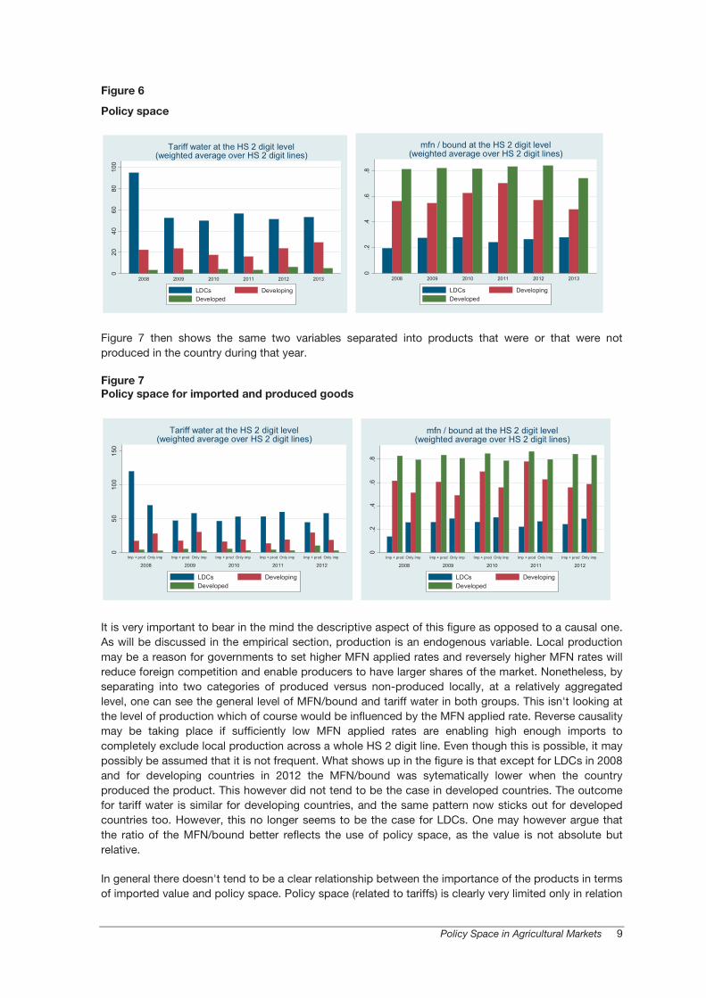
Figure 6 looks at the MFN/bound and tariff water from 2008 to 2013 for all three income level groups.

One can see that there hasn't been a drastic change of the space between the MFN applied and the

bound rate over the last five years except for the large decrease of tariff water between 2008 and 2009

in LDCs, most likely reflecting a wave of protectionism due to the financial and economic crisis.

0.1

.2.3

.4

Developed Developing LDCs

Share of imports from partners of RTAs

No food security Food security


Figure 6

Policy space

Figure 7 then shows the same two variables separated into products that were or that were not

produced in the country during that year.

Figure 7

Policy space for imported and produced goods

It is very important to bear in the mind the descriptive aspect of this figure as opposed to a causal one.

As will be discussed in the empirical section, production is an endogenous variable. Local production

may be a reason for governments to set higher MFN applied rates and reversely higher MFN rates will

reduce foreign competition and enable producers to have larger shares of the market. Nonetheless, by

separating into two categories of produced versus non-produced locally, at a relatively aggregated

level, one can see the general level of MFN/bound and tariff water in both groups. This isn't looking at

the level of production which of course would be influenced by the MFN applied rate. Reverse causality

may be taking place if sufficiently low MFN applied rates are enabling high enough imports to

completely exclude local production across a whole HS 2 digit line. Even though this is possible, it may

possibly be assumed that it is not frequent. What shows up in the figure is that except for LDCs in 2008

and for developing countries in 2012 the MFN/bound was sytematically lower when the country

produced the product. This however did not tend to be the case in developed countries. The outcome

for tariff water is similar for developing countries, and the same pattern now sticks out for developed

countries too. However, this no longer seems to be the case for LDCs. One may however argue that

the ratio of the MFN/bound better reflects the use of policy space, as the value is not absolute but

relative.

In general there doesn't tend to be a clear relationship between the importance of the products in terms

of imported value and policy space. Policy space (related to tariffs) is clearly very limited only in relation

020

4060

8010

0

2008 2009 2010 2011 2012 2013

Tariff water at the HS 2 digit level(weighted average over HS 2 digit lines)


0.2

.4.6

.8

2008 2009 2010 2011 2012 2013

mfn / bound at the HS 2 digit level(weighted average over HS 2 digit lines)


050

100

150

2008 2009 2010 2011 2012

Imp + prod Only imp Imp + prod Only imp Imp + prod Only imp Imp + prod Only imp Imp + prod Only imp

Tariff water at the HS 2 digit level(weighted average over HS 2 digit lines)


0.2

.4.6

.8

2008 2009 2010 2011 2012

Imp + prod Only imp Imp + prod Only imp Imp + prod Only imp Imp + prod Only imp Imp + prod Only imp

mfn / bound at the HS 2 digit level(weighted average over HS 2 digit lines)



to developed countries' imports. For LDCs there is virtually no imports for which policy space is not

available. In general, policy space for developing countries is often available but to a different degree

depending on specific products and countries. An important question that emerges from this analysis is

why policy space seems to be used in some cases but not in others. This may be due to the protection

of domestic production, food security and participation in global value chains. This question is

addressed in the empirical section.

4. EMPIRICAL SPECIFICATION

The first step is to run regressions on tariff water and available space at the HS 2 digit level using the

two measures presented in section 3. They are complemented by two measures that take into account

the presence of prohibitive tariffs that are below the bound rate and for the presence of preferential

tariffs. This is consistent with studies such as Foletti et al. (2011), and the reason is that countries won't

increase their MFN applied rate above the prohibitive rate. This means that the implicit bound is the

prohibitive rate and not the official bound rate in these cases. The preferential rate is below the MFN

applied rate and the country is tied to its contractual agreements, making increases of these rates

particularly complicated.

These two extra measures used are called true available space and true tariff water and are presented

in equations (3) and (4). The true tariff water uses the idea of dammed water found in Foletti et al. (2011),

where the prohibitive tariff is used when it is below the bound rate instead of using the bound rate itself,

and where the whole expression is multiplied by the share of imports taking place under a PTA. This

will therefore reduce tariff water if there is at least some trade taking place under a PTA, and reduces it

to zero in the most extreme case where all trade takes place under a PTA. The same idea is used to

create true available policy space. In this case the prohibitive rate is also used in place of the bound

rate when relevant, and the whole expression is multiplied by 1 minus the share of imports taking place

under a PTA in order to give us the loss of space due to PTAs. This loss of space is added to the initial

available space (including the prohibitive rates). This will lead to a higher value, meaning less available

space, with the extreme case being that the true MFN/bound is equal to 1 if all trade takes place under

a PTA.

��4�� 5 ��(,�,6 =∑ ��",�,7∗ ��",8,�,7∑ ��",�,7∗ ��",8,�,78∋9 :min:$��(,>,�,6; @��(,>,�,6A − ��(,>,�A ∗(1 − BCDE��",8,�,7 ��",8,�,7>∋F )(3)

��4� * �+ ,+�-. /��(,�,6 = H 2��(,�,6 ∗ 3��(,>,�,6∑ 2��(,�,6 ∗ 3��(,>,�,6>∋F I ��(,>,�,6min:$��(,>,�,6; @��(,>,�,6AJ>∋F

+

H 3@��(,>,�,63��(,>,�,6 ) ∗ I1 −H 2��(,�,6 ∗ 3��(,>,�,6∑ 2��(,�,6 ∗ 3��(,>,�,6>∋F I ��(,>,�,6min:$��(,>,�,6; @��(,>,�,6AJ>∋F J>∋F (4)

2��(,� is the import demand elasticity of a given HS 6 digit product in country c, 3��(,>,� are the imports of country c from country d for the same product, $��(,>,� is the bound rate, ��(,>,� the MFN applied tariff , and finally @��(,>,� the level of the prohibitive tariff, computed following Foletti et al. (2011), with @��(,>,� = ��(,>,� +MN0��",8,��",� .


The mean levels of elasticity within a given HS 2 digit line are taken by weighting by the value of

imports and the share of intermediates is computed in the same way. For the two explained variables,

namely tariff water and available space, the mean is computed as in equations (5) and (6), using

imports as well as the elasticity of import demand as weights, this time aggregating over HS 6 digit line

products also.

��4�� 5 ��,�,6 =∑ 6COD6PC%EEQP6DC��",�,7∗��",�,7∗ ��",�,7∑ ��",�,7∗ ��",�,7��"∋��(∋�� (5)

��4� * �+ ,+�-. /��,�,6 =∑ 6CODPRP%SPTSD�UP�D��",�,7∗��",�,7∗ ��",�,7∑ ��",�,7∗ ��",�,7��"∋��(∋�� (6)

True tariff water will be bound between 0 and the classical tariff water measure. Concerning true

available space, its value will be between the classical available space and 1. These two variables will

be the explained variables, as shown in equation (7) which shows the empirical specification used:

V��,�,6 = W + X2��,�,6 +Y�Z��[�\� ��-�� + ]�^^\-�/4��_�� + `.�^\4/��^Z�� + a�,6 +b��,�,6 (7)

where V��,�,6 will either be tariff water or available space. 2��,� is as before the import demand elasticity of a given HS 6 digit product in country c which is aggregated to the HS 2 digit level using import

values as weights. Intermediates is the trade weighted share of HS 6 digit products that are used as

intermediates in the production process within a given HS 2 digit product category. Food security is a

dummy variable that takes a value of 1 if the product, as mentioned above, is considered important

from a food security perspective, namely cereals and oils, fats as well as sugars, which correspond to

HS 2 digit categories 10, 15 and 17. Production is a dummy variable that takes a value of 1 if the good

was produced in the country in the same year and 0 otherwise. The choice of a dummy rather than the

value of production is clearly preferred in order to diminish the problematic endogeneity of the latter,

without obviously overcoming it entirely. It is unlikely that there isn't at least one producer who stays on

the market in the case of an MFN applied decrease. New producers starting to produce a product

following an increase of the MFN applied will certainly happen, but it would be quite rare at that level of

aggregation to observe a change on a whole HS 2 digit line. Finally, a�6 are country-year fixed effects and b��,�,6 is the error term. As the fixed effects are interacted, they not only control for anything specific to a given year or country, but also anything that is specific to a country in a given year. This

controls for the macroeconomic variables mentioned above, amongst which one can mention GDP,

inflation, the exchange rate and fiscal needs. Their expected influence on tariffs is reviewed below so

as to have a comprehensive view of what is influencing tariffs. Increased GDP will tend to increase

overall demand, therefore impacting consumer surplus. Inflation will tend to decrease producers' profits

due to products being relatively more expensive with respect to imports. This will in turn influence

demand for imports, increasing tariff revenue and influencing consumer surplus. The exchange rate will

change the price of imports, therefore influencing consumer surplus, tariff revenue due to a change in

the imported value and/or volume, and also producer profits due to a change in competitiveness. A

country's fiscal needs will influence the level of tariff revenue to aim for.

The interest for the food security variable and intermediates doesn't enable us to use item specific fixed

effects. Results of Ordinary Least Squares Regressions (OLS) run on equation (7) are presented in

Table 1. One must bear in mind that the OLS estimations for available space are biased due to the fact

that the explained variable is a fraction. This issue is explained and treated below, but the results of the

OLS regression are still presented as a reference in Table 1. Papke and Wooldridge (1996, 2008) show

why the bounded nature of a fraction and the possibility of observing values at the boundaries causes

estimation issues. More specifically, the effect of a given explanatory variable cannot be constant over

the whole range of values that it can take. Bluhm (2013) proposes a QMLE Stata routine entitled


fhetprob to perform a fractional probit estimation with heteroskedasticity based on the work of Papke

and Wooldridge (2008).7 In the present case, as in Bluhm (2013), time averages of all explanatory

variables are included in order to account for unobserved heterogeneity in the form of Correlated

Random Effects (CRE). The length of each spell is also included in the estimation and this is considered

potentially endogenous. Spell lengths of 1 must be dropped in order to avoid perfect collinearity

between the variable and its mean, as explained in Wooldridge (2008). Year dummies are also included

and errors are clustered by product. The results of this procedure are presented in columns 5 and 6 of

Table 1.

Table 1

OLS and fractional heteroskedastic probit

water

true

water MFN/bound

true

MFN/bound MFN/bound

true

MFN/bound

OLS OLS Fractional Heterosk. Probit

elasticity 0.006 0.055*** -0.000 -0.003*** -0.001 -0.024*

(0.24) (5.76) (-1.10) (-7.71) (-0.60) (-1.70)

intermediate 2.333*** -3.191*** -0.169*** -0.209*** -0.237*** -0.284***

(4.97) (-20.47) (-32.50) (-30.89) (-3.09) (-3.22)

food security 3.173*** 0.786*** 0.014** 0.014* 0.068 0.027

(4.33) (3.87) (2.24) (1.83) (0.50) (0.22)

production dummy

-0.890* -0.366** -0.005 -0.013** -0.002 0.137***

(-1.76) (-2.11) (-1.00) (-1.99) (-0.13) (4.58)

constant 1.206* 1.668*** 0.807*** 1.024*** -1.890 -1.750***

(1.87) (5.92) (17.94) (53.46) (-1.57) (-4.61)

country x year dummies

Yes Yes Yes Yes No No

year dummies Yes Yes Yes Yes Yes Yes

spell dummies No No No No Yes Yes

N 9774 9676 9774 9676 9601 9502

R2 0.783 0.437 0.594 0.451

t statistics in parentheses * p<0.10, ** p<0.05, *** p<0.01

The results discussed below look both at tariff water and use of policy space, for which the reference is

the fractional heteroskedastic probit. Results are mostly consistent with the OLS case but there are

some exceptions and as discussed higher up the OLS is potentially biased and is shown for

transparency and reference. As can be seen in Table 1, the elasticity does not seem to play a role in the

setting of tariff water or the MFN/bound (for which the term use of policy space is used below).

However, the effect for true tariff water is positive and significant and for the use of policy space it is

negative and significant. One must remember that higher values of tariff water are associated with

7 Papke and Wooldridge (1996) put forward that this issue is very similar to the case of models with binary data. They propose, based on Gourieroux, Montfort, and Trognon (1984) as well as McCullagh and Nelder (1989) to use Bernouilli Quasi Maximum Likelihood Estimator (QMLE), arguing that it is easy to maximize and is a member of the linear exponential family and consistent. Papke and Wooldridge (2008) note that when in the presence of panel data, there is an extra problem as one must be sure that standard errors are robust to arbitrary serial correlation and on top of that one must address the fact the fact that the explanatory variables may be correlated to unobserved heterogeneity. They suggest the use of a probit rather than an logit estimator, which even though often very similar, has the advantage of better handling endogenous variables. The method they propose is however not adapted to unbalanced panel data. This issue is solved in

Bluhm (2013), who proposes a QMLE Stata routine entitled fhetprob to perform a fractional probit estimation with heteroskedasticity based on the work of Papke and Wooldridge (2008). Bluhm (2013) explains that the conditional variance has to be able to vary with the nature of the unbalancedness, therefore requiring heteroskedasticity in the model.


lower ratios of the use of policy space, such that opposite signs on the coefficients of both variables

are consistent. The coefficients on intermediates are positive for tariff water and negative for the use of

policy space. The latter is also negative when considering the alternative true measure of the use of

policy space. It is negative for true tariff water, which contrasts with the other coefficients. Reasons for

this could be lower prohibitive rates in intermediate goods or more trade in intermediates with

preferential trade agreement partners. Except for this, results for intermediates are consistent with the

prior that the policymaker is keeping the price of inputs low to favor local production of processed

products. Products that are important in terms of food security tend to have more tariff water and true

tariff water. The use of policy space is not significantly affected by this variable in the fractional

heteroskedastic probit regressions, which is the preferred method due to the potential bias using OLS.

The coefficients on the production dummy tell us that when the country is producing the good there is

less tariff water and less true tariff water, for the use of policy space there is no significant effect and for

the true use of policy space it is positive (in the fractional heteroskedastic probit specification). This

suggests some protection of local producers.

In order to determine whether the effects of the different variables vary by income levels, regressions are run on three different samples, one for each income level. Even if there aren't necessarily strong

priors on the differences one may expect, reasons for believing that there may be differences include the fact that wealthier governments may have more technical skills to set MFN applied levels according to given economic conditions and item specificities, and poorer countries may give more importance to

issues such as food security. Results of these regressions are given in tables 2 to 4.

Table 2

Water and true water by income group (OLS)

Water

LDCs

Water

Developing

Water

Developed

True water

LDCs

True water

Developing

True water

Developed

elasticity 0.096*** -0.008 0.032 0.207*** 0.053*** 0.010***

(2.78) (-0.29) (1.20) (4.93) (5.06) (3.40)

intermediate 7.623*** 0.720 1.586 -8.026*** -2.045*** -0.162

(6.22) (1.33) (1.39) (-19.49) (-12.11) (-0.99)

food security -4.614*** 5.216*** 7.346*** 0.813* 0.932*** -0.257

(-2.60) (6.06) (3.67) (1.68) (3.91) (-0.91)

production dummy -4.540*** -0.145 2.211 -1.255** -0.118 -0.157

(-3.47) (-0.25) (1.62) (-2.22) (-0.69) (-1.03)

constant 51.930*** 1.286* 5.126*** 33.770*** 1.154*** 1.214***

(6.78) (1.76) (4.66) (6.03) (5.38) (8.05)


Yes Yes Yes Yes Yes Yes

N 1965 6781 756 1965 6781 756

R2 0.734 0.744 0.445 0.316 0.434 0.129



Table 3

MFN/bound and true MFN/bound by income group (OLS)

MFN/bound

LDCs

MFN/bound

Developing

MFN/bound

Developed

True

MFN/bound

LDCs

True

MFN/bound

Developing

True

MFN/bound

Developed

elasticity -0.001** -0.000 0.001 -0.007*** -0.003*** 0.001 (-2.43) (-1.04) (0.90) (-4.31) (-6.84) (0.77)

intermediate -0.163*** -0.176*** -0.158*** -0.112*** -0.239*** -0.235*** (-21.44) (-26.13) (-7.10) (-9.06) (-28.56) (-8.49)

food security 0.054*** 0.004 0.008 0.030** 0.008 0.044 (4.22) (0.49) (0.40) (2.12) (0.81) (1.51)

production dummy

-0.010 -0.005 -0.017 -0.018 -0.011 -0.020 (-1.11) (-0.75) (-0.77) (-1.49) (-1.37) (-0.77)

constant 0.375*** 0.820*** 0.307*** 0.419*** 1.035*** 0.687*** (4.99) (17.98) (8.88) (2.58) (49.88) (10.44)


Yes Yes Yes Yes Yes Yes

N 1965 6781 756 1965 6781 756 R2 0.415 0.578 0.675 0.205 0.483 0.510


Table 4

MFN/bound and true MFN/bound by income group (Fract. Heter. Probit)

MFN/bound

LDCs

MFN/bound

Developing

MFN/bound

Developed

True

MFN/bound

LDCs

True

MFN/bound

Developing

True

MFN/bound

Developed

elasticity -0.012*** 0.001 -0.017*** -0.055 -0.022 -0.010*** (-3.47) (1.30) (-3.25) (-1.56) (-1.44) (-2.77)

intermediate -0.262* -0.242*** -0.647 -0.176 -0.477*** -1.016 (-1.72) (-2.64) . (-1.30) (-3.62) (-1.62)

food security 0.202 0.024 -0.141 0.120 -0.027 -0.027 (1.60) (0.19) (-0.68) (0.98) (-0.21) (-0.18) production dummy

-0.017 -0.007 0.160** 0.081* 0.289*** 0.307*

(-0.94) (-0.30) (2.09) (1.73) (6.67) (1.78)

constant -1.801*** -1.475*** -6.009*** -0.404 -1.144*** -5.430***

(-3.11) (-3.63) (-4.67) (-1.07) (-3.59) (-3.76)

year dummies Yes Yes Yes Yes Yes Yes spell dummies Yes Yes Yes Yes Yes Yes

N 1982 6859 760 1965 6781 756


The elasticity of import demand coefficient for tariff water is positive and significant only for LDCs, but

for true water it is positive and significant for all income groups. The effect remains the largest in LDCs,

followed by developing and developed countries. When looking at the use of policy space (once again

in the fractional heteroskedastic probit specification) the effect is negative for LDCs and developed

countries and for the true use only in developed countries. As was shown in the descriptive statistics,

there tends to be considerably more water in LDCs, in particular due to high bound rates. This may

explain this pattern in which the effect on water sticks out for LDCs whereas it is more the case for the

use of policy space in developed countries. The coefficient on intermediates is only positive in LDCs,

and as in the regression with all regions together, this sign switches for true water and it is also

negative for true water in developing countries. It is negative for the use of policy space in both these


income regions and only significant and negative for its true counterpart in developing countries. The

coefficient on food security indicates that there is less tariff water in products related to food security in

LDCs but more water in developed and developing countries. The sign changes for LDCs when

considering true tariff water, which can have two potential explanations, on one hand prohibitive rates

may tend to be higher in food products due to the goods being of primary necessity, and on the other

hand, as illustrated in Figure 5 and discussed in section 3, there is more trade taking place with PTA

partners in non-food security related products in LDCs. For other income groups the difference is only

very slight, and in the opposite way. It could help explain the coefficient for developed countries going

from positive and significant to non-significant. Food security doesn't seem to be related to the use of

policy space, probably meaning that for food security products it is the absolute levels of the MFN

applied and the bound rates that are playing a role. Finally, the production dummy coefficient tells us

that tariff water and true tariff water is lower in LDCs when the good is also produced by the country

but that there tends to be no difference for the two other income groups. For the true use of policy

space it is positive in all income groups.

5. ROBUSTNESS CHECKS

Regressions are run at a lower level of aggregation to check the consistency of results at the cost of

losing the production dummy. Results for regressions run at the HS 6 digit line level are shown in Table

5. Nearly all coefficients are consistent. There are two cases where the confidence level changes but

the coefficient remains significant and still of the same sign, namely food security in the OLS regression

on the true MFN/bound (column 4) and the import demand elasticity in the fractional heteroskedastic

regression once again for the true MFN/bound (column 6). The same coefficient but for the classical

MFN/bound goes from not significant in the HS 2 digit case to negative and significant (consistent with

the true MFN/bound coefficient) in the HS 6 digit case. Finally, food significance went from being non-

significant for the HS 2 digit to positive and significant for the HS 6 digit true MFN/bound specification

(column 6).

Table 5

OLS and fractional heteroskedastic probit at the HS 6 digit level

water true water MFN/bound

true

MFN/bound MFN/bound

true

MFN/bound


elasticity -0.004 0.034*** 0.000 -0.001*** -0.005*** -0.009** (-1.03) (22.86) (0.55) (-15.40) (-4.25) (-2.17) intermediate 3.303*** -2.606*** -0.120*** -0.138*** -0.315*** -0.445*** (15.20) (-32.66) (-64.26) (-55.54) (-8.17) (-9.69) food security 3.097*** 0.766*** 0.005** 0.029*** -0.002 0.117** (13.07) (6.18) (2.16) (8.95) (-0.06) (2.1) constant 0.511** 1.800*** 0.848*** 0.949*** -0.335*** -2.151*** (2.16) (10.26) (54.97) (82.60) (-6.45) (-3.86)



year dummies Yes Yes Yes Yes Yes Yes spell dummies No No No No Yes Yes

N 66801 62898 66801 62898 65129 60952 R2 0.623 0.306 0.558 0.407



Table 6

OLS and fractional heteroskedastic probit excluding the import demand elasticity

water true water MFN/bound

true

MFN/bound MFN/bound

true

MFN/bound


intermediate 2.330*** -3.221*** -0.169*** -0.208*** -0.239*** -0.281***

(4.96) (-20.58) (-32.49) (-30.57) (-3.14) (-2.95)

food security 3.175*** 0.806*** 0.014** 0.013* 0.069 0.024

(4.32) (3.96) (2.23) (1.71) (0.52) (0.21)

production dummy -0.892* -0.394** -0.005 -0.011* -0.004 0.131***

(-1.77) (-2.28) (-0.98) (-1.77) (-0.23) (4.51)

constant 1.201* 1.616*** 0.807*** 1.027*** -1.987** -1.852***

(1.86) (5.76) (17.95) (53.36) (-2.06) (-5.22)



year dummies Yes Yes Yes Yes Yes Yes

spell dummies No No No No Yes Yes

N 9774 9676 9774 9676 9601 9502

R2 0.783 0.433 0.594 0.446


Another concern that one may have is the use of the import demand elasticity as an explanatory

variable. The reason for this is that it is also used in the weighting of the explained variables. Table 6

shows the main results run without this variable. All results are consistent with coefficients that are all

of the same sign and level of significance in all specifications, except for the production dummy in the

OLS regression run on the true use of policy space (column 4), for which the confidence level goes

from 5 percent to 10 percent.


6. CONCLUSION

This paper investigates the extent of policy flexibility and its use in relation to tariff setting in agricultural

products. To this end, the magnitude of flexibility - the policy space countries have under international

commitments - is measured by the difference between the bound rate and the MFN applied rate. The

use of policy space is measured by the ratio of the MFN applied to the bound rate. Using econometric

methods this study analyzes whether policy space is influenced by four specific factors: the elasticity of

import demand of the product, the use of the product as an intermediate good, whether the product is

important for food security, and whether the product is also domestically produced.

A general finding is that policy space in agricultural products is generally available, and only limited for

developed countries. Many developing countries have ample room to raise tariffs in most agricultural

imports without infringing binding commitments. For LDCs there is virtually no imports for which policy

space is not available. The findings indicate that four specific factors are related to the use of policy

space. In particular, policy space tends to be used relatively less for products with lower elasticity of

demand. This is consistent with relatively higher rates of protection on elastic products. The results also

find that policy space is seldom used for intermediate products. This may suggest that processing

industries are lobbying governments to keep taxation relatively lower on intermediate products. In

regard of products relevant for food security, the results find that policy space is larger but that there is

no difference in its use. This suggests two things. First, governments may be aiming for access to

cheaper food products, therefore helping consumer welfare. Second, governments may retain policy

space so as to increase the MFN applied in case of need. In regard to products that face domestic

competitors, the results indicate lower tariff water and more use of policy space, suggesting that

producer protection is an issue related to the level of policy space to use and the level of market

protection to set. When looking at the results for different country groupings, it appears that for LDCs,

the overall results are similar to the results with all income groups. They even tend to be larger in

magnitude for the availability of policy space. Results for developing countries indicate that although

the four main factors still play a role, they do so to a lesser extent. For developed countries there is a

similar tendency, despite intermediates no longer playing a significant role.

Overall, the main message of this paper is that most developing countries retain a large degree of

policy space as the MFN applied rates are usually well below the bound rates. Policymakers seem to

be basing the choice of the applied tariffs on a number of product-specific variables that seemingly

correspond to a complex mixture of optimization of consumer surplus, producer profits and fiscal

needs, all this associated with the fact that governments preferably want to have some available space

in order to be able to adjust to any future economic shocks. The impact of the different variables on

policy space seems stronger in LDCs, but especially when considering tariff water. This tendency is

less pronounced for the use of policy space. As a final caveat, it is important to underline that the

analysis does not take into account any policy restrictions on the use of non-tariff measures. Indeed,

one interesting path for future research would be to explore whether policy space is limited by some of

these types of trade policy instruments.


BIBLIOGRAPHY

Amador, M. and K. Bagwell (2012), "Tariff Revenue and Tariff Caps", American Economic Review,

102(3), 459-65.

Bacchetta, M. and Piermartini, R. (2011), "The Value of Bindings", WTO staff working paper.

Bluhm, R. (2013), "fhetprob: A fast qmle stata routine for fractional probit models with multiplicative Heteroskedasticity", Forthcoming as UNU-MERIT working paper.

Estevadeordal, A., C. Freund and E. Ornelas (2008), "Does regionalism affect trade liberalization toward

nonmembers?", The Quarterly Journal of Economics, 123(4), 1531-75.

Foletti, L., M. Fugazza, A. Nicita and M. Olarreaga (2011), "Smoke in the (Tariff) Water", The World

Economy, 34(2), 248-64.

Francois J. and W. Martin (2004), "Commercial Policy Variability, Bindings and Market Access",

European Economic Review, 48(3), 665-79.

Gourieroux, C., A. Monfort and A. Trognon (1984), "Pseudo-maximum likelihood methods: theory",

Econometrica, 52(3), 681-00.

Handley, K. (2014), "Exporting under trade policy uncertainty: Theory and evidence", Journal of

International Economics, 94(1), 50-66.

Horn, H., G. Maggi and R. Staiger (2010), "Trade Agreements as Endogenously Incomplete Contracts",

American Economic Review, 100(1), 394-419.

Humphrey, J. and Memedovic, O. (2006), "Global Value Chains in the Agrifood Sector", UNIDO Working Paper Series, UNIDO Strategic Research and Economics Branch, United Nations

Industrial Development Organization.

Kee, H.L., A. Nicita and M. Olarreaga (2009), "Estimating Trade Restrictiveness Indices", Economic

Journal, 119(534), 172-99.

McCullagh, P. and J. A. Nelder (1989), Generalized Linear Models, 2nd edition, Chapman and Hall, New

York.

Multilateral Trade Negotiations on Agriculture - A Resource Manual (2000), Part 2 - Agreement on

Agriculture, Module 2 - Preparing for Negotiating Further Reductions of the Bound Tariffs, R. Sharma - Commodities and Trade Division, Food and Agriculture Organization of the United Nations, Rome.

Organisation for Economic Co-operation and Development (2012), "Mapping Global Value Chains",

Policy Dialogue on Aid for Trade, Trade and Agricultural Directorate and Trade Committee, The OECD Conference Centre, Paris.

Papke, E. and J. Wooldridge (1996), "Econometric Methods for Fractional Response Variables with an

Application to 401 (K) Plan Participation Rates", Journal of Applied Econometrics, 11(6), 619-32.

Papke, E. and J. Wooldridge (2008), "Panel Data Methods for Fractional Response Variables with an

Application to Test Pass Rates", Journal of Econometrics, 145(1-2), 121-33.

Sala D., Schroder P.H. and E. Yalcin (2009), "Market Access through Bound Tariffs", Scottish Journal of

Political Economy, 57(3), 272-89.

U n i t e d n at i o n s C o n f e r e n C e o n t r a d e a n d d e v e l o p m e n t


POLICY ISSUES IN INTERNATIONAL TRADE AND COMMODITIESRESEARCH STUDY SERIES No. 73

Printed at United Nations, Geneva1600845 (E) – January 2016 – 245

UNCTAD/ITCD/TAB/75

United Nations publicationISSN 1607-8291

Policy Space in Agricultural Markets -...

Documents

Transcript of Policy Space in Agricultural Markets -...