POLI di MI tecnicolano Numerical Simulation of Aero-Servo-Elastic Problems, with Application to Wind...
33
POLI POLI di di MI MI tecnico tecnico lano lano Numerical Simulation of Aero-Servo-Elastic Problems, with Application to Wind Turbines and Rotary Wing Vehicles Carlo L. Bottasso Politecnico di Milano COMPDYN 2007 Rethymno, Crete, Greece, June 13-15, 2007
-
date post
20-Dec-2015 -
Category
Documents
-
view
215 -
download
1
Transcript of POLI di MI tecnicolano Numerical Simulation of Aero-Servo-Elastic Problems, with Application to Wind...
PO
LIPO
LI
di
di M
IM
Itecn
ico
tecn
ico
lano
lanoNumerical Simulation of
Aero-Servo-Elastic Problems, with Application to Wind Turbines and
Rotary Wing Vehicles
Carlo L. BottassoPolitecnico di Milano
COMPDYN 2007 Rethymno, Crete, Greece, June 13-15, 2007
Numerical Simulation of Aero-Servo-Elastic Problems, with Application to Wind Turbines and
Rotary Wing Vehicles
Carlo L. BottassoPolitecnico di Milano
COMPDYN 2007 Rethymno, Crete, Greece, June 13-15, 2007
Aero
-Serv
o-E
last
icit
y o
f R
oto
rcra
ftA
ero
-Serv
o-E
last
icit
y o
f R
oto
rcra
ftA
ero
-Serv
o-E
last
icit
y o
f R
oto
rcra
ftA
ero
-Serv
o-E
last
icit
y o
f R
oto
rcra
ft
POLITECNICO di MILANO DIA
AcknowledgementsAcknowledgements
Work in collaboration with:
A. Croce, D. Leonello, L. Riviello, B. Savini;
Work supported by:
AgustaWestland, US Army Research Office, Leitner S.p.A.

Aero
-Serv
o-E
last
icit
y o
f R
oto
rcra
ftA
ero
-Serv
o-E
last
icit
y o
f R
oto
rcra
ftA
ero
-Serv
o-E
last
icit
y o
f R
oto
rcra
ftA
ero
-Serv
o-E
last
icit
y o
f R
oto
rcra
ft
POLITECNICO di MILANO DIA
OutlineOutline
• Multidisciplinary FEM-based multibody modeling;
• Active control of complex aero-servo-elastic models: three challenging applications;
• Adaptive identification of reduced models;
• Examples;
• Conclusions and outlook.
Aero
-Serv
o-E
last
icit
y o
f R
oto
rcra
ftA
ero
-Serv
o-E
last
icit
y o
f R
oto
rcra
ftA
ero
-Serv
o-E
last
icit
y o
f R
oto
rcra
ftA
ero
-Serv
o-E
last
icit
y o
f R
oto
rcra
ft
POLITECNICO di MILANO DIA
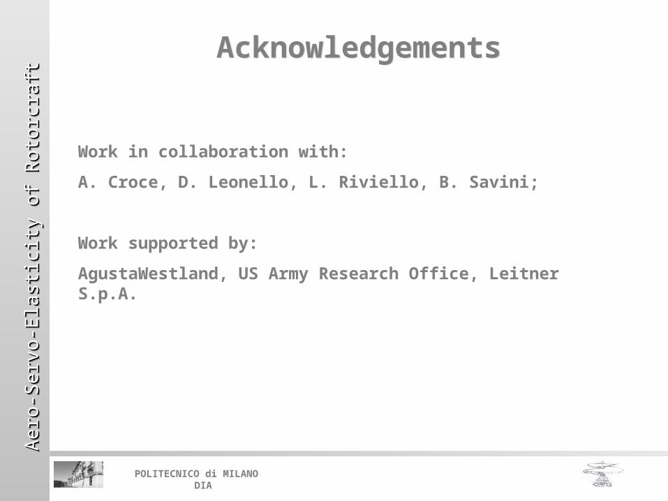
Multidisciplinary FEM Multibody Modeling
Multidisciplinary FEM Multibody Modeling
Rotorcraft aeroelastic model: finite element multibodyfinite element multibody code (Bauchau & Bottasso 2001).
Highlights: arbitrarily complexarbitrarily complex topologies, non-linearly non-linearly stablestable energy decaying schemes.
Aerodynamic models: lifting lines; inflow models (Pitt-Peters, Peters-He); free-wake; CFD.
Other models: controllers; actuators (hydraulic, engine, etc.); sensors; unilateral contact.

Aero
-Serv
o-E
last
icit
y o
f R
oto
rcra
ftA
ero
-Serv
o-E
last
icit
y o
f R
oto
rcra
ftA
ero
-Serv
o-E
last
icit
y o
f R
oto
rcra
ftA
ero
-Serv
o-E
last
icit
y o
f R
oto
rcra
ft
POLITECNICO di MILANO DIA
Multidisciplinary FEM Multibody Modeling
Multidisciplinary FEM Multibody Modeling

Aero
-Serv
o-E
last
icit
y o
f R
oto
rcra
ftA
ero
-Serv
o-E
last
icit
y o
f R
oto
rcra
ftA
ero
-Serv
o-E
last
icit
y o
f R
oto
rcra
ftA
ero
-Serv
o-E
last
icit
y o
f R
oto
rcra
ft
POLITECNICO di MILANO DIA
Some Trends and NeedsSome Trends and Needs
• Integration of complex multi-physics models with active active controlscontrols (e.g., add virtual pilots to vehicle models, systematically explore operational envelope boundaries, etc.);
• Model reductionModel reduction (e.g., for model-based control);
• Model identificationModel identification from experimental data;
• Real-timeReal-time performance (e.g., for pilot-in-the-loop applications).
Aero
-Serv
o-E
last
icit
y o
f R
oto
rcra
ftA
ero
-Serv
o-E
last
icit
y o
f R
oto
rcra
ftA
ero
-Serv
o-E
last
icit
y o
f R
oto
rcra
ftA
ero
-Serv
o-E
last
icit
y o
f R
oto
rcra
ft
POLITECNICO di MILANO DIA
Three challenging applications :
• Simulation of maneuvers (Maneuvering Multibody Simulation of maneuvers (Maneuvering Multibody Dynamics, MMBD);Dynamics, MMBD);
• Finding periodic solutions (“trimming”);
• Control of wind turbine generators.
Active Control of Complex Aero-Servo-Elastic ModelsActive Control of Complex Aero-Servo-Elastic Models
Aero
-Serv
o-E
last
icit
y o
f R
oto
rcra
ftA
ero
-Serv
o-E
last
icit
y o
f R
oto
rcra
ftA
ero
-Serv
o-E
last
icit
y o
f R
oto
rcra
ftA
ero
-Serv
o-E
last
icit
y o
f R
oto
rcra
ft
POLITECNICO di MILANO DIA
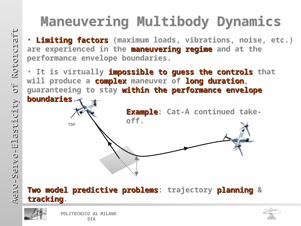
• Limiting factorsLimiting factors (maximum loads, vibrations, noise, etc.) are experienced in the maneuvering regimemaneuvering regime and at the performance envelope boundaries.
• It is virtually impossible to guess the controlsimpossible to guess the controls that will produce a complexcomplex maneuver of long durationlong duration, guaranteeing to stay within the performance envelope boundarieswithin the performance envelope boundaries.
Maneuvering Multibody DynamicsManeuvering Multibody Dynamics
TDP
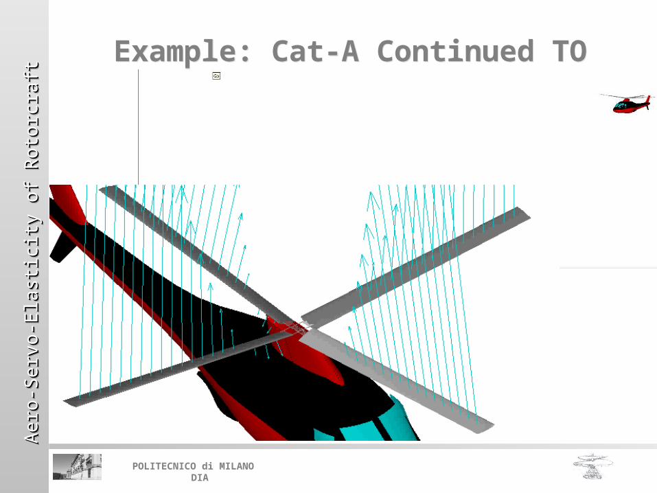
ExampleExample: Cat-A continued take-off.
Two model predictive problemsTwo model predictive problems: trajectory planningplanning & trackingtracking.

Aero
-Serv
o-E
last
icit
y o
f R
oto
rcra
ftA
ero
-Serv
o-E
last
icit
y o
f R
oto
rcra
ftA
ero
-Serv
o-E
last
icit
y o
f R
oto
rcra
ftA
ero
-Serv
o-E
last
icit
y o
f R
oto
rcra
ft
POLITECNICO di MILANO DIA
Maneuvering Multibody DynamicsManeuvering Multibody Dynamics
Aero
-Serv
o-E
last
icit
y o
f R
oto
rcra
ftA
ero
-Serv
o-E
last
icit
y o
f R
oto
rcra
ftA
ero
-Serv
o-E
last
icit
y o
f R
oto
rcra
ftA
ero
-Serv
o-E
last
icit
y o
f R
oto
rcra
ft
POLITECNICO di MILANO DIA
Example: Cat-A Continued TOExample: Cat-A Continued TO

Aero
-Serv
o-E
last
icit
y o
f R
oto
rcra
ftA
ero
-Serv
o-E
last
icit
y o
f R
oto
rcra
ftA
ero
-Serv
o-E
last
icit
y o
f R
oto
rcra
ftA
ero
-Serv
o-E
last
icit
y o
f R
oto
rcra
ft
POLITECNICO di MILANO DIA
MMBD: Model Predictive Planning & Tracking
MMBD: Model Predictive Planning & Tracking
1. Maneuver planning problem (reduced model)
Reference trajectory2. Tracking
problem (reduced model)
Trajectory flown by comprehensive model
4. Reduced model update
Predictive solutions
3. Steering problem (comprehensive model)
Prediction window
Steering window
Tracking cost
Prediction error
Prediction window
Tracking cost
Steering window
Prediction error
Tracking costPrediction window
Steering window
Prediction error
5. Re-plan with updated reduced model
Updated reference trajectory
Reference trajectory
Fly the comprehensive modelcomprehensive model along the reference trajectory and, at the same time, updateupdate the reduced model (learning).

Aero
-Serv
o-E
last
icit
y o
f R
oto
rcra
ftA
ero
-Serv
o-E
last
icit
y o
f R
oto
rcra
ftA
ero
-Serv
o-E
last
icit
y o
f R
oto
rcra
ftA
ero
-Serv
o-E
last
icit
y o
f R
oto
rcra
ft
POLITECNICO di MILANO DIA
Three challenging applications :
• Simulation of maneuvers (Maneuvering Multibody Dynamics, MMBD);
• Finding periodic solutions (“trimming”);Finding periodic solutions (“trimming”);
• Control of wind turbine generators.
Active Control of Complex Aero-Servo-Elastic ModelsActive Control of Complex Aero-Servo-Elastic Models
Aero
-Serv
o-E
last
icit
y o
f R
oto
rcra
ftA
ero
-Serv
o-E
last
icit
y o
f R
oto
rcra
ftA
ero
-Serv
o-E
last
icit
y o
f R
oto
rcra
ftA
ero
-Serv
o-E
last
icit
y o
f R
oto
rcra
ft
POLITECNICO di MILANO DIA
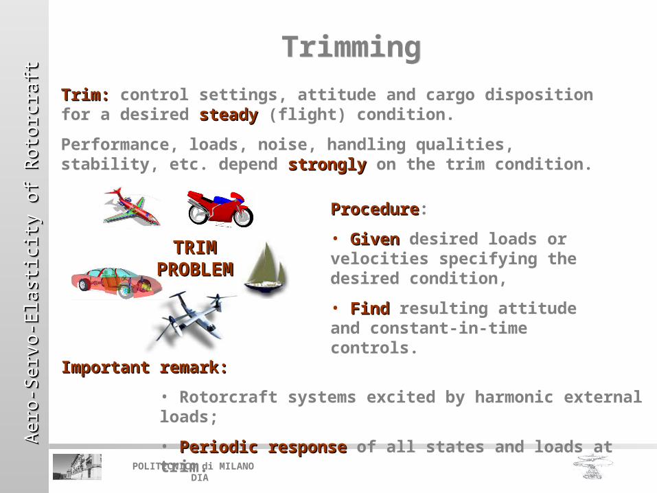
ProcedureProcedure:
• GivenGiven desired loads or velocities specifying the desired condition,
• FindFind resulting attitude and constant-in-time controls.
TrimmingTrimming
Trim:Trim: control settings, attitude and cargo disposition for a desired steadysteady (flight) condition.
Performance, loads, noise, handling qualities, stability, etc. depend stronglystrongly on the trim condition.
Important remark: Important remark:
• Rotorcraft systems excited by harmonic external loads;
• Periodic response Periodic response of all states and loads at trim.
TRIM TRIM PROBLEPROBLE
MM
Aero
-Serv
o-E
last
icit
y o
f R
oto
rcra
ftA
ero
-Serv
o-E
last
icit
y o
f R
oto
rcra
ftA
ero
-Serv
o-E
last
icit
y o
f R
oto
rcra
ftA
ero
-Serv
o-E
last
icit
y o
f R
oto
rcra
ft
POLITECNICO di MILANO DIA
Formulation of Rotorcraft Trim Problem
Formulation of Rotorcraft Trim Problem
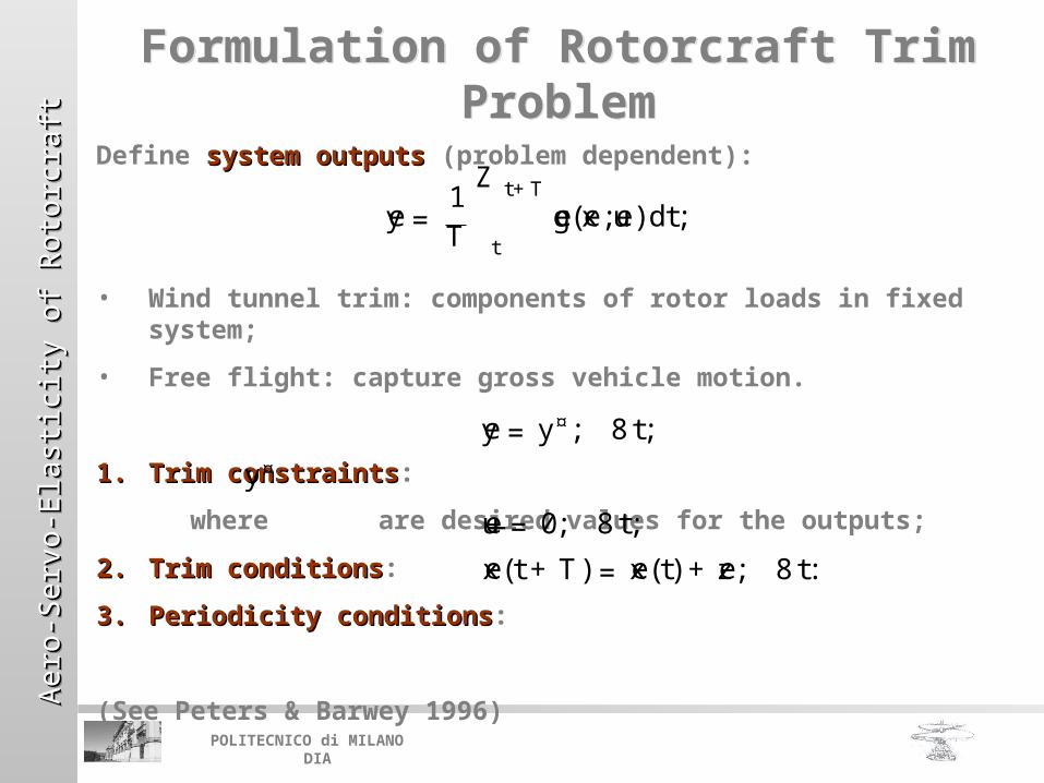
Define system outputssystem outputs (problem dependent):
• Wind tunnel trim: components of rotor loads in fixed system;
• Free flight: capture gross vehicle motion.
1.1. Trim constraintsTrim constraints:
where are desired values for the outputs;
2.2. Trim conditionsTrim conditions:
3.3. Periodicity conditionsPeriodicity conditions:
(See Peters & Barwey 1996)
y¤
ey = y¤; 8t;
_eu = 0; 8t;
ex(t + T) = ex(t) + ez; 8t:
ey =1T
Z t+T
teg(ex; eu)dt;
Aero
-Serv
o-E
last
icit
y o
f R
oto
rcra
ftA
ero
-Serv
o-E
last
icit
y o
f R
oto
rcra
ftA
ero
-Serv
o-E
last
icit
y o
f R
oto
rcra
ftA
ero
-Serv
o-E
last
icit
y o
f R
oto
rcra
ft
POLITECNICO di MILANO DIA
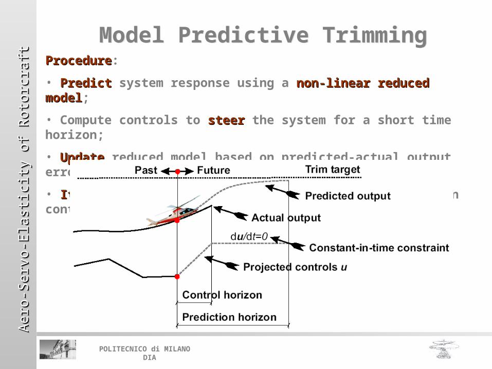
Model Predictive TrimmingModel Predictive TrimmingProcedureProcedure:
• PredictPredict system response using a non-linear reduced modelnon-linear reduced model;
• Compute controls to steersteer the system for a short time horizon;
• UpdateUpdate reduced model based on predicted-actual output errors;
• IterateIterate, shifting prediction forward (receding horizon control).

Aero
-Serv
o-E
last
icit
y o
f R
oto
rcra
ftA
ero
-Serv
o-E
last
icit
y o
f R
oto
rcra
ftA
ero
-Serv
o-E
last
icit
y o
f R
oto
rcra
ftA
ero
-Serv
o-E
last
icit
y o
f R
oto
rcra
ft
POLITECNICO di MILANO DIA
Three challenging applications :
• Simulation of maneuvers (Maneuvering Multibody Dynamics, MMBD);
• Finding periodic solutions (“trimming”);
• Control of wind turbine generators.Control of wind turbine generators.
Active Control of Complex Aero-Servo-Elastic ModelsActive Control of Complex Aero-Servo-Elastic Models
Aero
-Serv
o-E
last
icit
y o
f R
oto
rcra
ftA
ero
-Serv
o-E
last
icit
y o
f R
oto
rcra
ftA
ero
-Serv
o-E
last
icit
y o
f R
oto
rcra
ftA
ero
-Serv
o-E
last
icit
y o
f R
oto
rcra
ft
POLITECNICO di MILANO DIA
Control of Wind Turbine GeneratorsControl of Wind Turbine Generators
Target value
Predicted output
Actual output
Projected controls u
d du/ t=0
Past Future
t
t+T Prediction horizonp
t+T Steering windows
t+T Control horizonc
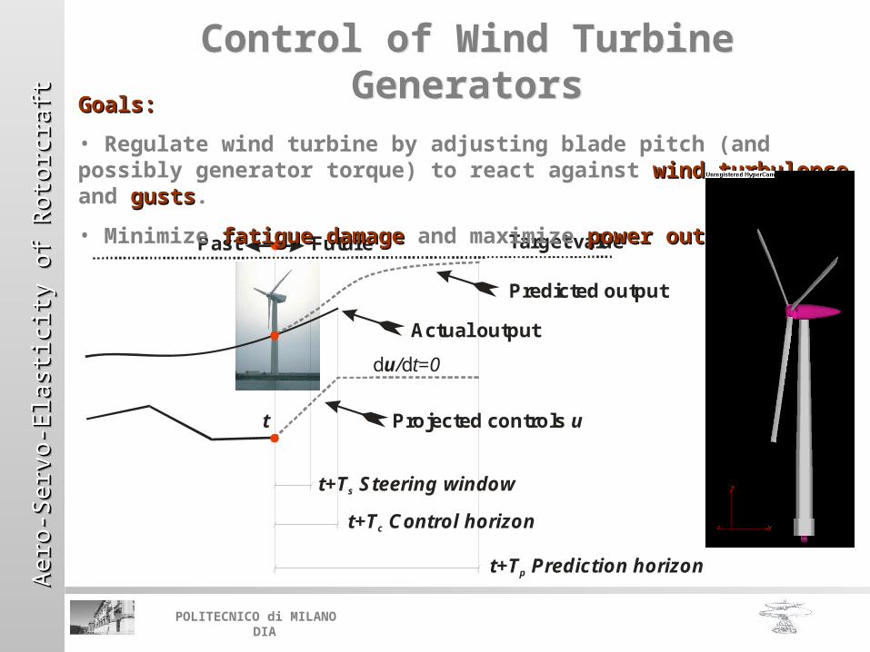
Goals: Goals:
• Regulate wind turbine by adjusting blade pitch (and possibly generator torque) to react against wind turbulencewind turbulence and gustsgusts.
• Minimize fatigue damagefatigue damage and maximize power outputpower output.

Aero
-Serv
o-E
last
icit
y o
f R
oto
rcra
ftA
ero
-Serv
o-E
last
icit
y o
f R
oto
rcra
ftA
ero
-Serv
o-E
last
icit
y o
f R
oto
rcra
ftA
ero
-Serv
o-E
last
icit
y o
f R
oto
rcra
ft
POLITECNICO di MILANO DIA
Reduced modelReduced model: few dofs, captures gross to-be-controlled response.
Comprehensive Comprehensive multibody-based modelmultibody-based model: many dofs, captures fine scale solution details.
Reduced Model IdentificationReduced Model Identification
System
System
Identifica
tio
Identifica
tio
nn
This procedure is common This procedure is common to all three previous to all three previous problems.problems.
Aero
-Serv
o-E
last
icit
y o
f R
oto
rcra
ftA
ero
-Serv
o-E
last
icit
y o
f R
oto
rcra
ftA
ero
-Serv
o-E
last
icit
y o
f R
oto
rcra
ftA
ero
-Serv
o-E
last
icit
y o
f R
oto
rcra
ft
POLITECNICO di MILANO DIA
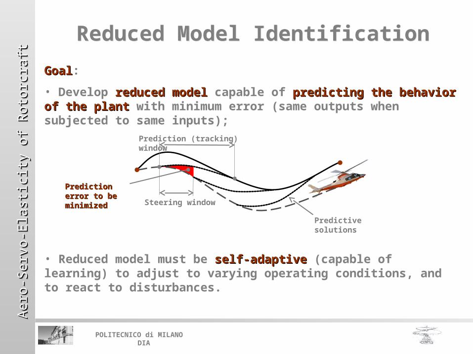
GoalGoal:
• Develop reduced modelreduced model capable of predicting the behavior predicting the behavior of the plantof the plant with minimum error (same outputs when subjected to same inputs);
• Reduced model must be self-adaptiveself-adaptive (capable of learning) to adjust to varying operating conditions, and to react to disturbances.
Predictive solutions
Prediction (tracking) window
Steering window
Prediction Prediction error to be error to be minimizedminimized
Reduced Model IdentificationReduced Model Identification
Aero
-Serv
o-E
last
icit
y o
f R
oto
rcra
ftA
ero
-Serv
o-E
last
icit
y o
f R
oto
rcra
ftA
ero
-Serv
o-E
last
icit
y o
f R
oto
rcra
ftA
ero
-Serv
o-E
last
icit
y o
f R
oto
rcra
ft
POLITECNICO di MILANO DIA
Reduced Model IdentificationReduced Model Identification
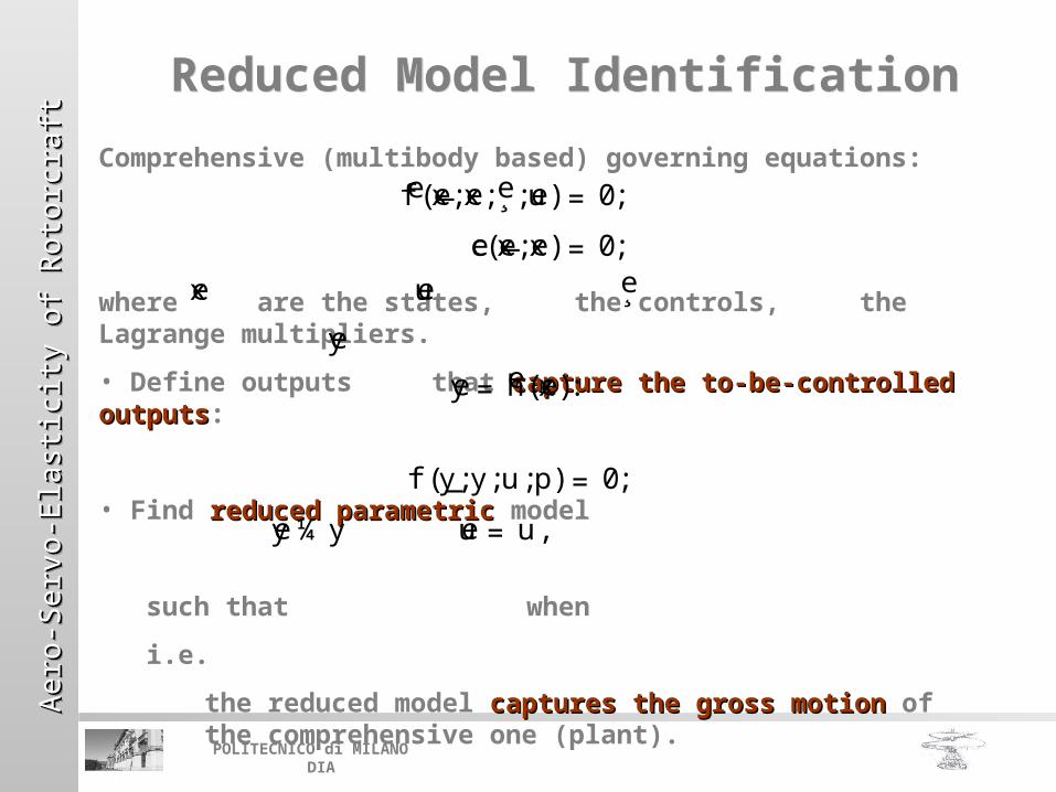
Comprehensive (multibody based) governing equations:
where are the states, the controls, the Lagrange multipliers.
• Define outputs that capture the to-be-controlled capture the to-be-controlled outputsoutputs:
• Find reduced parametricreduced parametric model
such that when
i.e.
the reduced model captures the gross motioncaptures the gross motion of the comprehensive one (plant).
euex e
ey = eh(ex):
ef ( _ex; ex; e; eu) = 0;
ec( _ex; ex) = 0;
f ( _y;y;u;p) = 0;
ey
ey ¼y eu = u,

Aero
-Serv
o-E
last
icit
y o
f R
oto
rcra
ftA
ero
-Serv
o-E
last
icit
y o
f R
oto
rcra
ftA
ero
-Serv
o-E
last
icit
y o
f R
oto
rcra
ftA
ero
-Serv
o-E
last
icit
y o
f R
oto
rcra
ft
POLITECNICO di MILANO DIA
Reduced Model FormulationReduced Model Formulation
Neural augmented reference modelNeural augmented reference model:
• Reference (problem dependent) analytical modelReference (problem dependent) analytical model:
For example, in this work:
- Rotorcraft problems: 2D rigid body model, actuator-disk rotor (blade element theory + uniform inflow).
= CG position & velocity, pitch & pitch rate, rotor speed;
= main & tail rotor collective, lateral & longitudinal cyclics, available power.
- Wind turbine problems: actuator-disk rotor + springs to model tower flexibility.
= rotor speed, tower tip position & velocity;
= blade pitch, generator torque.
f ref( _y;y;u) = 0;
y
u
y
u
Aero
-Serv
o-E
last
icit
y o
f R
oto
rcra
ftA
ero
-Serv
o-E
last
icit
y o
f R
oto
rcra
ftA
ero
-Serv
o-E
last
icit
y o
f R
oto
rcra
ftA
ero
-Serv
o-E
last
icit
y o
f R
oto
rcra
ft
POLITECNICO di MILANO DIA
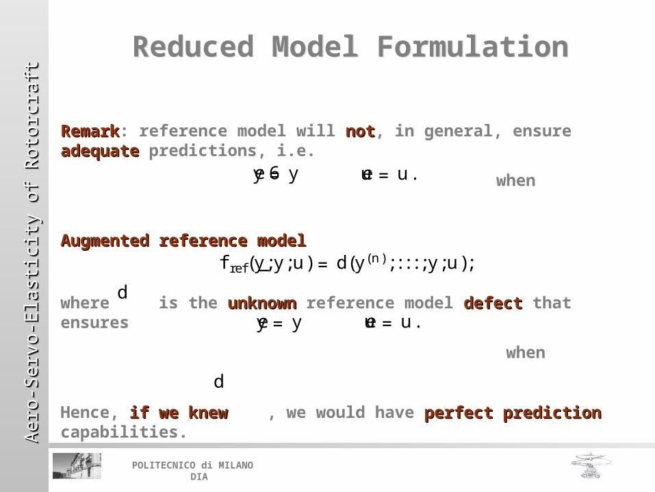
Reduced Model FormulationReduced Model Formulation
RemarkRemark: reference model will notnot, in general, ensure adequateadequate predictions, i.e.
when
Augmented reference modelAugmented reference model
where is the unknownunknown reference model defectdefect that ensures
when
Hence, if we knewif we knew , we would have perfect predictionperfect prediction capabilities.
d
f ref( _y;y;u) = d(y(n); : : : ;y;u);
eu = u.
eu = u.ey 6= y
ey = y
d
Aero
-Serv
o-E
last
icit
y o
f R
oto
rcra
ftA
ero
-Serv
o-E
last
icit
y o
f R
oto
rcra
ftA
ero
-Serv
o-E
last
icit
y o
f R
oto
rcra
ftA
ero
-Serv
o-E
last
icit
y o
f R
oto
rcra
ft
POLITECNICO di MILANO DIA
Reduced Model FormulationReduced Model Formulation
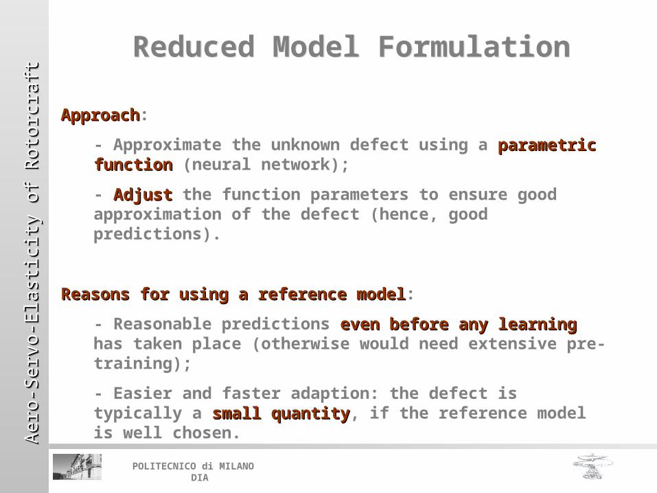
ApproachApproach:
- Approximate the unknown defect using a parametric parametric functionfunction (neural network);
- AdjustAdjust the function parameters to ensure good approximation of the defect (hence, good predictions).
Reasons for using a reference modelReasons for using a reference model:
- Reasonable predictions even before any learningeven before any learning has taken place (otherwise would need extensive pre-training);
- Easier and faster adaption: the defect is typically a small quantitysmall quantity, if the reference model is well chosen.
Aero
-Serv
o-E
last
icit
y o
f R
oto
rcra
ftA
ero
-Serv
o-E
last
icit
y o
f R
oto
rcra
ftA
ero
-Serv
o-E
last
icit
y o
f R
oto
rcra
ftA
ero
-Serv
o-E
last
icit
y o
f R
oto
rcra
ft
POLITECNICO di MILANO DIA
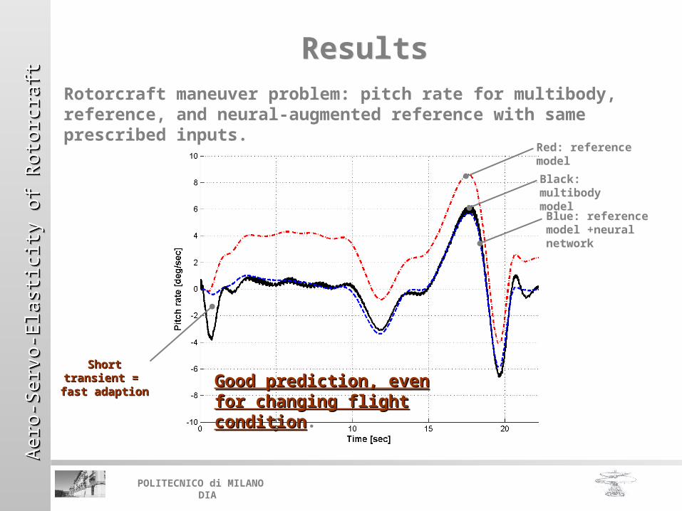
ResultsResultsRotorcraft maneuver problem: pitch rate for multibody, reference, and neural-augmented reference with same prescribed inputs.
Short Short transient = transient =
fast adaptionfast adaption
Black: multibody model
Red: reference model
Blue: reference model +neural network
Good prediction, even Good prediction, even for changing flight for changing flight conditioncondition.
Aero
-Serv
o-E
last
icit
y o
f R
oto
rcra
ftA
ero
-Serv
o-E
last
icit
y o
f R
oto
rcra
ftA
ero
-Serv
o-E
last
icit
y o
f R
oto
rcra
ftA
ero
-Serv
o-E
last
icit
y o
f R
oto
rcra
ft
POLITECNICO di MILANO DIA
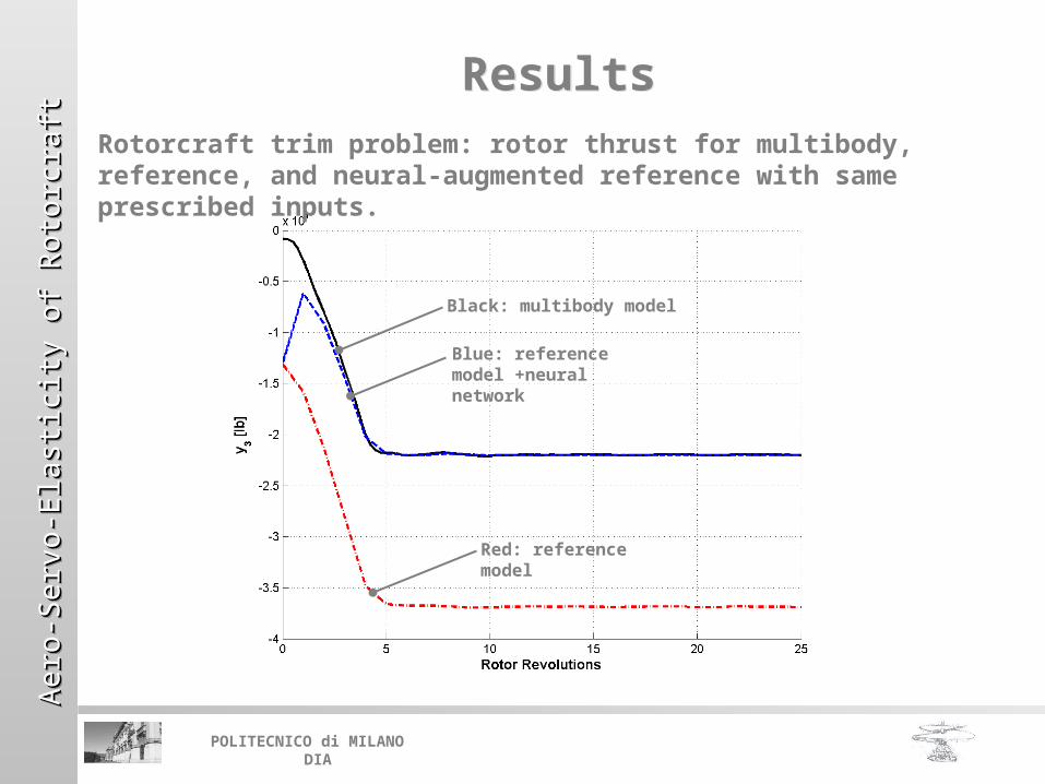
ResultsResultsRotorcraft trim problem: rotor thrust for multibody, reference, and neural-augmented reference with same prescribed inputs.
Black: multibody model
Red: reference model
Blue: reference model +neural network
Aero
-Serv
o-E
last
icit
y o
f R
oto
rcra
ftA
ero
-Serv
o-E
last
icit
y o
f R
oto
rcra
ftA
ero
-Serv
o-E
last
icit
y o
f R
oto
rcra
ftA
ero
-Serv
o-E
last
icit
y o
f R
oto
rcra
ft
POLITECNICO di MILANO DIA
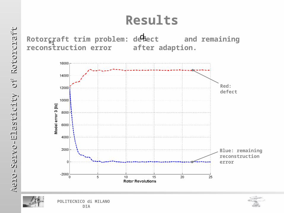
ResultsResultsRotorcraft trim problem: defect and remaining reconstruction error after adaption.
di"i
Red: defect
Blue: remaining reconstruction error
Aero
-Serv
o-E
last
icit
y o
f R
oto
rcra
ftA
ero
-Serv
o-E
last
icit
y o
f R
oto
rcra
ftA
ero
-Serv
o-E
last
icit
y o
f R
oto
rcra
ftA
ero
-Serv
o-E
last
icit
y o
f R
oto
rcra
ft
POLITECNICO di MILANO DIA
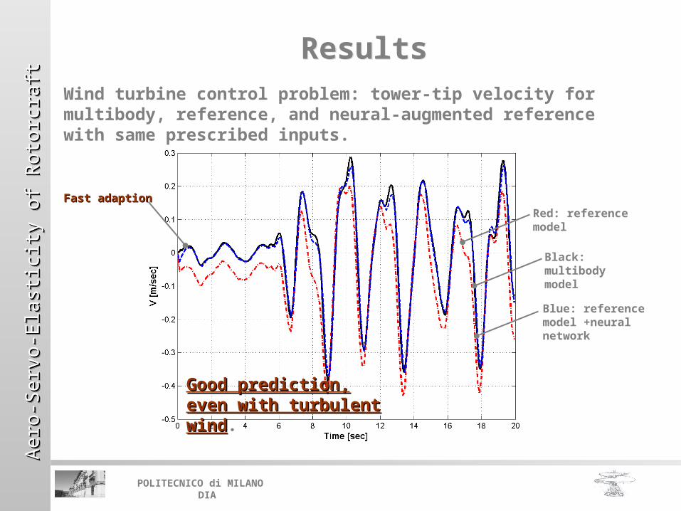
ResultsResultsWind turbine control problem: tower-tip velocity for multibody, reference, and neural-augmented reference with same prescribed inputs.
Black: multibody model
Red: reference model
Blue: reference model +neural network
Fast adaptionFast adaption
Good prediction, even Good prediction, even with turbulent windwith turbulent wind.
Aero
-Serv
o-E
last
icit
y o
f R
oto
rcra
ftA
ero
-Serv
o-E
last
icit
y o
f R
oto
rcra
ftA
ero
-Serv
o-E
last
icit
y o
f R
oto
rcra
ftA
ero
-Serv
o-E
last
icit
y o
f R
oto
rcra
ft
POLITECNICO di MILANO DIA
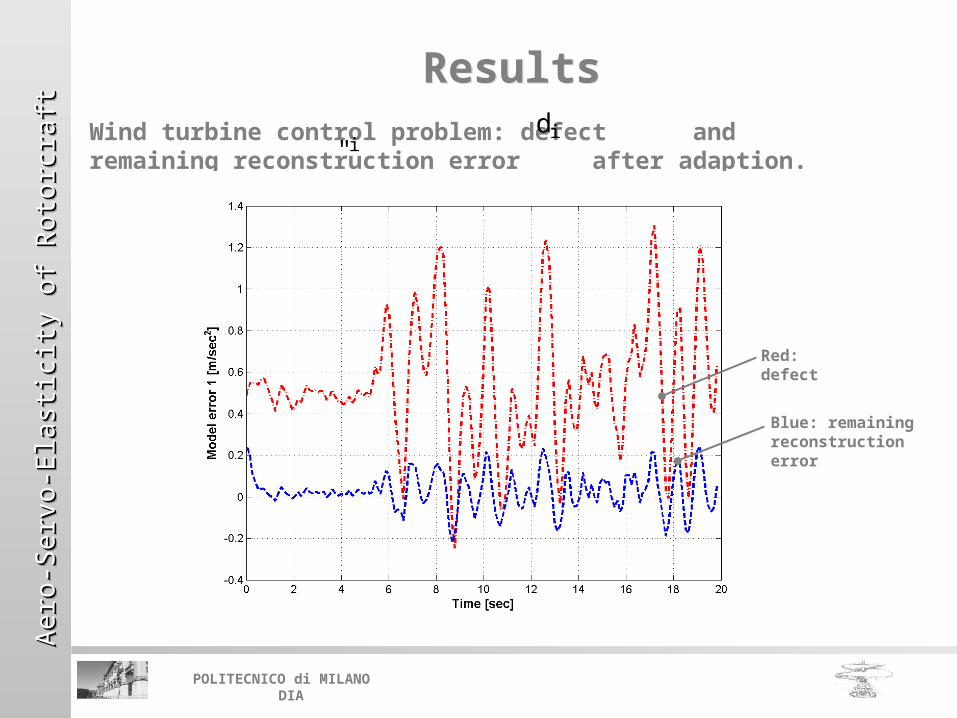
ResultsResultsWind turbine control problem: defect and remaining reconstruction error after adaption.
di"i
Red: defect
Blue: remaining reconstruction error

Aero
-Serv
o-E
last
icit
y o
f R
oto
rcra
ftA
ero
-Serv
o-E
last
icit
y o
f R
oto
rcra
ftA
ero
-Serv
o-E
last
icit
y o
f R
oto
rcra
ftA
ero
-Serv
o-E
last
icit
y o
f R
oto
rcra
ft
POLITECNICO di MILANO DIA
Optimal Control ProblemOptimal Control Problem (with unknown internal event at T1)
• Cost function:
• Constraints and bounds:
- Initial trimmed conditions at 30 m/s
- Power limitations
Application: Rotorcraft Minimum Time Obstacle Avoidance
Application: Rotorcraft Minimum Time Obstacle Avoidance

Aero
-Serv
o-E
last
icit
y o
f R
oto
rcra
ftA
ero
-Serv
o-E
last
icit
y o
f R
oto
rcra
ftA
ero
-Serv
o-E
last
icit
y o
f R
oto
rcra
ftA
ero
-Serv
o-E
last
icit
y o
f R
oto
rcra
ft
POLITECNICO di MILANO DIA
Minimum Time Obstacle AvoidanceMinimum Time Obstacle Avoidance
Aero
-Serv
o-E
last
icit
y o
f R
oto
rcra
ftA
ero
-Serv
o-E
last
icit
y o
f R
oto
rcra
ftA
ero
-Serv
o-E
last
icit
y o
f R
oto
rcra
ftA
ero
-Serv
o-E
last
icit
y o
f R
oto
rcra
ft
POLITECNICO di MILANO DIA
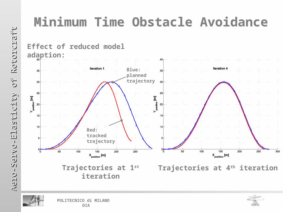
Minimum Time Obstacle AvoidanceMinimum Time Obstacle Avoidance
Trajectories at 1st iteration
Trajectories at 4th iteration
Effect of reduced model adaption:
Red: tracked trajectory
Blue: planned trajectory
Aero
-Serv
o-E
last
icit
y o
f R
oto
rcra
ftA
ero
-Serv
o-E
last
icit
y o
f R
oto
rcra
ftA
ero
-Serv
o-E
last
icit
y o
f R
oto
rcra
ftA
ero
-Serv
o-E
last
icit
y o
f R
oto
rcra
ft
POLITECNICO di MILANO DIA
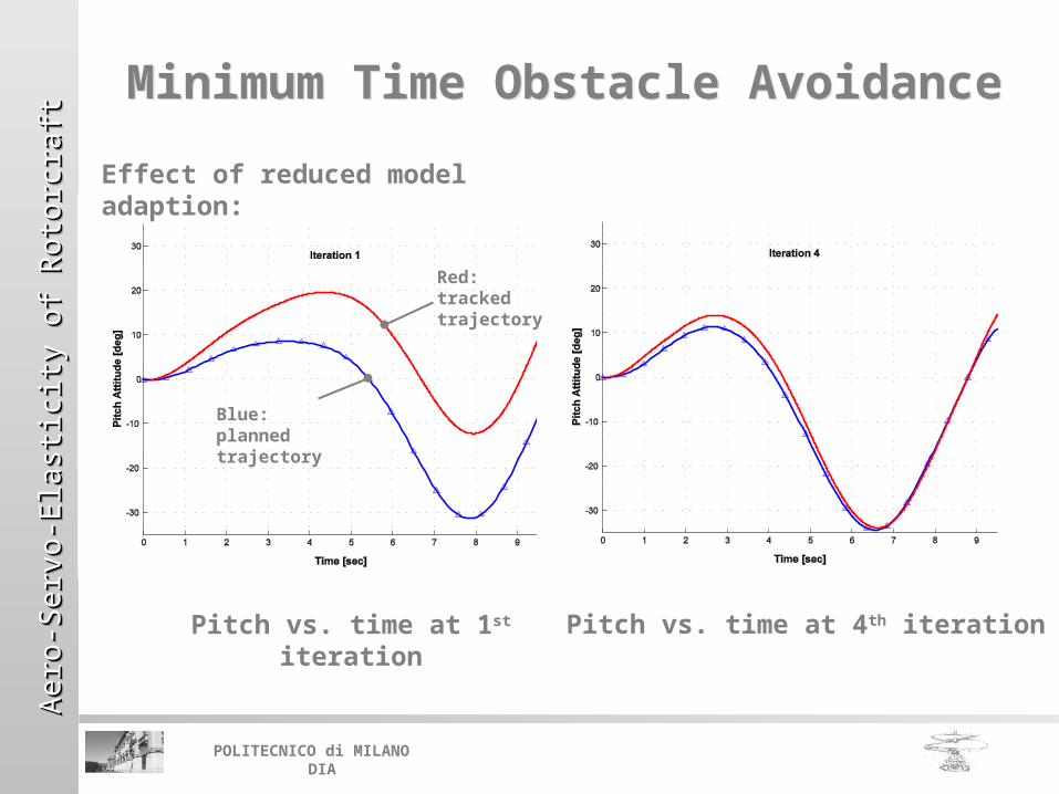
Minimum Time Obstacle AvoidanceMinimum Time Obstacle Avoidance
Pitch vs. time at 1st iteration
Pitch vs. time at 4th iteration
Effect of reduced model adaption:
Red: tracked trajectory
Blue: planned trajectory

Aero
-Serv
o-E
last
icit
y o
f R
oto
rcra
ftA
ero
-Serv
o-E
last
icit
y o
f R
oto
rcra
ftA
ero
-Serv
o-E
last
icit
y o
f R
oto
rcra
ftA
ero
-Serv
o-E
last
icit
y o
f R
oto
rcra
ft
POLITECNICO di MILANO DIA
ConclusionsConclusions
Observations:
• Computational procedures now blend traditionally separate disciplines, e.g. aero-servo-elasticityaero-servo-elasticity with flight flight mechanicsmechanics;
• Mathematical models of vehicles are becoming so so complexcomplex that there is a trend to use methods for analyzing experimental dataexperimental data (e.g. stability analysis, system identification, etc.);
Outlook:
• These trends will continue (virtual lab);
• Real-time simulation;
• Human behavior models.