C.S. Verbeek

Polar Auxin Transport in Arabidopsis

Inflorescence Stems

Bachelor thesis, August 22, 2013

Supervisor: Dr. S.C. Hille

Mathematical Institute of Leiden University

Contents

1 Introduction 2

2 Underlying Information 32.1 Biology . . . . . . . . . . . . . . . . . . . . . . . . . . . . . . . . 32.2 Experimental Set-up(s) and Results . . . . . . . . . . . . . . . . 4

3 Preparations: Cellular Level Models 63.1 Effective Number Flux between Adjacent Cells . . . . . . . . . . 63.2 Intracellular Transport . . . . . . . . . . . . . . . . . . . . . . . . 9

4 Cell Array Models 134.1 Fast Homogenization within Cells . . . . . . . . . . . . . . . . . . 134.2 A Model with Intracellular Diffusion and Active Transport . . . 154.3 A Continuum Approximation for fast Homogenization . . . . . . 16

5 Steady State Analysis 185.1 Case of Intracellular Diffusion . . . . . . . . . . . . . . . . . . . . 185.2 Case of Intracellular Diffusion and Transport . . . . . . . . . . . 225.3 Case of Intracellular Mixing . . . . . . . . . . . . . . . . . . . . . 265.4 Examining Exponential ’Blow-up’ in Detail . . . . . . . . . . . . 27

6 Discussion and Conclusions 32

A Parameter values 33

B Matlab Simulation 34B.1 Parameters.m . . . . . . . . . . . . . . . . . . . . . . . . . . . . . 34B.2 conc.m . . . . . . . . . . . . . . . . . . . . . . . . . . . . . . . . . 34B.3 Auxplot.m . . . . . . . . . . . . . . . . . . . . . . . . . . . . . . . 35

C Examining equation (13) 36

1

1 Introduction

This thesis is about the polar auxin transport in Arabidopsis thaliana inflores-cence stems. It is made in collaboration with the Plant BioDynamics Laboratoryin Leiden, where the experiments mentioned in this thesis were done.In this thesis we investigate the inter- and intracellular transport of auxin. Thereason for this is that we want to know more about how auxin is transported.Is this done by simple diffusion in the cell or is there active transport? Whichtransporters in the cell membrane play a role and what is their transport ca-pacity? The problem with this is that the auxin molecule, indole-3-acetic acid,is very small and therefore not visible. It can’t be made visible either, e.g. bylabelling with a fluorescent protein.Our attempt to learn more about this transport in Arabidopsis thaliana is tolook at auxin at a macroscopic level. This is possible by making the auxin ra-dioactive. It is not as accurate as looking at visible molecules, but it is accurateenough for this macroscopic level. With modelling we try to fit the obtainedexperimental results. Assumptions will be made and tested in this thesis by thismodelling.One of the most elaborate articles about this subject is that of G.J. Mitchison,[8], dating back to the 1980s. In the following three decades the mathematicalmodelling of polar auxin transport in stem segments seems to have stalled. Re-search seems to have shifted to the molecular biology of the system, with a fewexceptions, [3, 5]. This article was used as a starting point and improved at thePlant BioDynamics Laboratory. This thesis is a sub-question of the researchthat is being done there.This thesis will differ from most other mathematical theses, because of the bio-logical nature of the subject. As such it is located in the field of mathematicalbiology. It is meant to be readable for both mathematicians and experimentalbiologists with some mathematical training.

2

2 Underlying Information

2.1 Biology

Arabidopsis thaliana is a small flowering plant that, like any other plant, trans-ports auxin, indole-3-acetic acid (IAA), through it’s tissue. Auxin is a phyto-hormone that regulates growth, rates of cell expansion and rates of cell divisionand establishment and maintenance of pattern during growth and development,like a morphogen, [2, 7]. In this thesis we will look at auxin as a molecule andits function is not relevant.The transport of auxin is confined to transport channels. One transport channelconsists of a single file of cells with an apoplast between every two adjacent cells.In the stem there are around 10 vascular bundles. The cross-sectional area ofthe stem is around 3, 7 × 10−7 m2 of which 0, 7 × 10−7 m2 consists of vascularbundles. Around 20 to 30 percent of this area of vascular bundles is expectedto consist of transport channels.IAA is a weak acid, with acidity constant pKa = 4.8. Thus it is present both inprotonated form (IAAH) and anion form (IAA−) at the same time. In the cellmembrane we have PIN-transporters and AUX-transporters to transport IAAthrough the membrane. PIN-transporters hypothetically transport IAA− out ofthe cell and AUX-transporters transport IAA− into the cell. PIN-transportersare mainly located in the membrane at the basal end of the cell and AUX-transporters are equally distributed across the membrane. The protonated formcan only diffuse through the membrane. The different forms of transport areassumed to be linear in the concentration of the solute they transport. That is,we assume that the concentrations if IAA are such that transport rates are inthe linear regime. No saturation effect needs to be taken into account.The fraction of IAA in each form are pH-dependent and can be computed fromthe Henderson-Hasselbalch equation:

pH = pKa + log10

[A−]

[HA].

The fraction of IAA in anion form as function of pH is then given by

f =1

1 + 10pKa−pH.

pH fraction anion fraction protonated4 0.1368 0.86325 0.6131 0.38697 0.9937 0.0063

We assume that the acidity in the cytoplasm and apoplast is buffered and there-fore constant. The fraction of auxin in anion form is in a chemical equilibrium.The constant acidity dictates then that the fraction of anion auxin is a constant,fa for the apoplast and fc for the cytoplasm of all cells.

3

There are no known carriers that can transport IAA in either form into a vac-uole and it is not likely to go in there by itself either, so the transport of IAAwithin the cell is exclusively through the cytoplasm.

2.2 Experimental Set-up(s) and Results

Indole-3-acetic acid (IAA) is a small molecule and therefore it is not visible. Itcan’t be made fluorescent either yet. So in the experiments, done in the PlantBioDynamics Laboratory in Leiden, tritium labelled IAA (3H-IAA) is used, sothe radioactivity can be measured in order to determine the total amount ofauxin in different sections of plant tissue. The tritium is located in the indolering. (See Figure 1)

Figure 1: IAA-molecule struc-ture.

Another possibility is using 14C labelled IAA.However, the carbon is typically located in theCOOH part of the auxin molecule. (See Fig-ure 1) This part can be split off, so this is notas accurate as tritium, which is in one of therings and can’t be cut off, since not only theradioactivity of the 14C attached to the auxinis measured, but also the radioactivity of the14C that has been cut off.Petri dishes filled with molten paraffin, inwhich grooves between a donor well and re-ceiver well were cut, were used for the exper-iments. The grooves had a length of 16 mmand in each groove a 16 mm inflorescence stemof the Arabidopsis was placed, with the api-cal side of the stem at the donor well. In thedonor well the tritium labelled IAA is addedwith a concentration of 1 × 10−7 M. The receiver well is filled with neutralbuffer and is emptied regularly at relatively short time intervals during the ex-periments, so the concentration of IAA (tritium labelled and unlabelled) in thereceiver well can be considered to remain approximately 0 M during the exper-iment. The total amount of 3H-IAA taken from the receiver well is measuredover time and after 600 minutes the stem is cut in 4 parts of 4 mm and theamount of 3H-IAA in each part is measured.An example of results of such experiments is shown in Figures 2 and 3. Fromthe slope of the asymptote as t → ∞ in Figure 2 we conclude that that thesteady state transport rate of IAA through the stem segment is approximately9× 10−3 fmol/s.

4

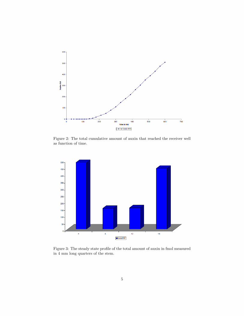
Figure 2: The total cumulative amount of auxin that reached the receiver wellas function of time.

Figure 3: The steady state profile of the total amount of auxin in fmol measuredin 4 mm long quarters of the stem.

5

3 Preparations: Cellular Level Models

It is convenient to do some preparations on cellular level before we continuemodelling the entire system.

3.1 Effective Number Flux between Adjacent Cells

Between every two cells there is an apoplast. To find an expression for theeffective number flux of auxin between cell i and cell i + 1, we first have toexamine the number fluxes between cell i and the apoplast and between theapoplast and cell i + 1. With the assumption that auxin is homogeneouslydistributed near the membranes ’connecting’ two cells, with the apoplast inbetween and that the auxin concentration in the apoplast is in quasi-steadystate, we can derive the following expressions:

νAUX(Ca) = PinAfaCa

νPIN (Ci) = PexAfcCi

J i,as (Ci, Ca) = PsA(1− fc)Ci − PsA(1− fa)Ca

= PsA(1− fc)(Ci −

1− fa1− fc

Ca

)Ja,i+1s (Ci+1, Ca) = −PsA(1− fc)

(Ci+1 −

1− fa1− fc

Ca

)where νAUX , νPIN , J i,as , Ja,i+1

s are the number fluxes of the AUX transporters,PIN transporters, diffusion over the left membrane and diffusion over the rightmembrane respectively, (recall that transport rates were assumed to be in thelinear regime),Ci, Ca, Ci+1 are the total concentration of auxin (anion and protonated auxin)in cell i, the apoplast and cell i + 1 respectively, the first and last close to themembrane,A is the area of the connecting cell membrane,Pin, Pex, Ps are the effective permeabilities by means of the AUX transporters,PIN transporters and simple diffusion respectively dependent only in the formof auxin they transport, i.e. anion or protonated form.Let Ji,a(Ci, Ca) and Ja,i+1(Ci+1, Ca) be the total number flux of auxin overthe membrane from cell i to the apoplast and from the apoplast to cell i + 1respectively, then

Ji,a(Ci, Ca) = J i,as (Ci, Ca) + νPIN (Ci)− νAUX(Ca)

= PsA(1− fc)(Ci −

1− fa1− fc

Ca

)+ PexAfcCi − PinAfaCa

Ja,i+1(Ci+1, Ca) = νAUX(Ca) + Ja,i+1s (Ci+1, Ca)

= PinAfaCa − PsA(1− fc)(Ci+1 −

1− fa1− fc

Ca

)

6

The assumption is made that Ca is in quasi-steady state, C?a . From thisfollows

Ji,a(Ci, C?a) = Ja,i+1(Ci+1, C

?a)

PsA(1− fc)(Ci −

1− fa1− fc

C?a

)+PexAfcCi − PinAfaC?a = PinAfaC

?a

−PsA(1− fc)(Ci+1 −

1− fa1− fc

C?a

)PsA(1− fc) (Ci + Ci+1) + PexAfcCi = 2PinAfaC

?a + 2PsA(1− fa)C?a

Ps(1− fc) (Ci + Ci+1) + PexfcCi = (2Pinfa + 2Ps(1− fa))C?a

C?a =Ps(1− fc) (Ci + Ci+1) + PexfcCi

2Pinfa + 2Ps(1− fa)

Define

Ps := Ps(1− fc)Pin := Pinfa

Pex := Pexfc

R :=1− fa1− fc

,

then we get

C?a =Ps (Ci + Ci+1) + PexCi

2Pin + 2PsR.

Since our quasi-steady state assumption implies that

Ji,a(Ci, C?a) = Ja,i+1(Ci+1, C

?a)

we can define Ji,i+1 := Ji,a(Ci, C?a) = Ja,i+1(Ci+1, C

?a) as the total number flux

of auxin between cell i and i+ 1.

7

We get

Ji,i+1 = Ji,a(Ci, C?a)

= PsA(1− fc)(Ci −

1− fa1− fc

C?a

)+ PexAfcCi − PinAfaC?a

= PsA(Ci − RC?a) + PexACi − PinAC?a

= PsA

(Ci − R

Ps (Ci + Ci+1) + PexCi

2Pin + 2PsR

)+ PexACi

−PinAPs (Ci + Ci+1) + PexCi

2Pin + 2PsR

=1

2Pin+2PsR[(2Pin+2PsR)PsACi−PsAR(Ps(Ci+Ci+1)+PexCi)

+(2Pin + 2PsR)PexACi − PinA(Ps(Ci + Ci+1) + PexCi)]

=A

2Pin + 2PsR[(P 2

s R) + PsPin + PsPexR+ PinPex)Ci

−(P 2s R+ PsPin)Ci+1)]

=A

2Pin + 2PsR[(Pin + PsR)(Ps + Pex)Ci − (Pin + PsR)PsCi+1]

=1

2PsA

[Ps + Pex

PsCi − Ci+1

]= −PA(Ci+1 −RCi),

where

P =1

2Ps

=1

2Ps(1− fc)

and

R =Ps + Pex

Ps

= 1 +Pexfc

Ps(1− fc).

Mitchison, [8], assumes the expression

Ji,i+1 = pCi + q(Ci − Ci+1)

for these fluxes. Thus,

q = PA, p = PA(R− 1).

8

Since the values of P and R may not be the same at the beginning and end ofthe stem, e.g. due to damage to cells caused by cutting process, we get

Ji,i+1 = −1

2PsA

(Ci+1 −

Ps + PexPs

Ci

)= −PA(Ci+1 −RCi), i ∈ {1, 2, . . . , N − 1}

Jin = −PinA(C1 −RinCd)Jout = −PoutA(Cr −RoutCN )

Cr=0= PoutRoutACN (1)

where Cd is the concentration of auxin in the donor well and Cr the concentra-tion in the receiver well.Note that this last Pin is not the same Pin as used before. The Pin = Pinfawill not return, since our expressions of Ji,i+1, Jin and Jout are not dependentof this Pin, so from now on every Pin will be the one as in (1).

3.2 Intracellular Transport

Diffusion is in all directions and not just in one. We have to deal with the threedimensions of the cells. Assume that the cells are cylindrical, with a cylindricalvacuole in the middle. Let l be the length of one cell, l − 2δ (0 < δ < l

2 ) thelength of the vacuole, R the radius of the cells and R − d(x) the radius of thevacuoles at point x in the cell. From this follows that the non-vacuole part ofthe radius equals R − (R − d(x)) = d(x). Let A(x) be the cross section of the

cytoplasm at x, i.e. A(x) = {(x, y, z)|R− d(x) <√y2 + z2 < R}.

Figure 4: The mathematical abstraction of a cell in a transport channel ofArabidopsis.

Let Ci(x, y, z, t) be the concentration of auxin in cell i in point (x, y, z) attime t. A change to cylindrical coordinates is convenient:

Ci(x, r, θ, t) = Ci(x, y, z, t)

9

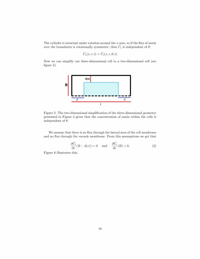
The cylinder is invariant under rotation around the x-axis, so if the flux of auxinover the boundaries is rotationally symmetric, then Ci is independent of θ:

Ci(x, r, t) = Ci(x, r, θ, t)

Now we can simplify our three-dimensional cell to a two-dimensional cell (seefigure 5).

Figure 5: The two-dimensional simplification of the three-dimensional geometrypresented in Figure 4 given that the concentration of auxin within the cells isindependent of θ.

We assume that there is no flux through the lateral area of the cell membraneand no flux through the vacuole membrane. From this assumptions we get that

∂Ci∂r

(R− d(x)) = 0 and∂Ci∂r

(R) = 0. (2)

Figure 6 illustrates this.

10

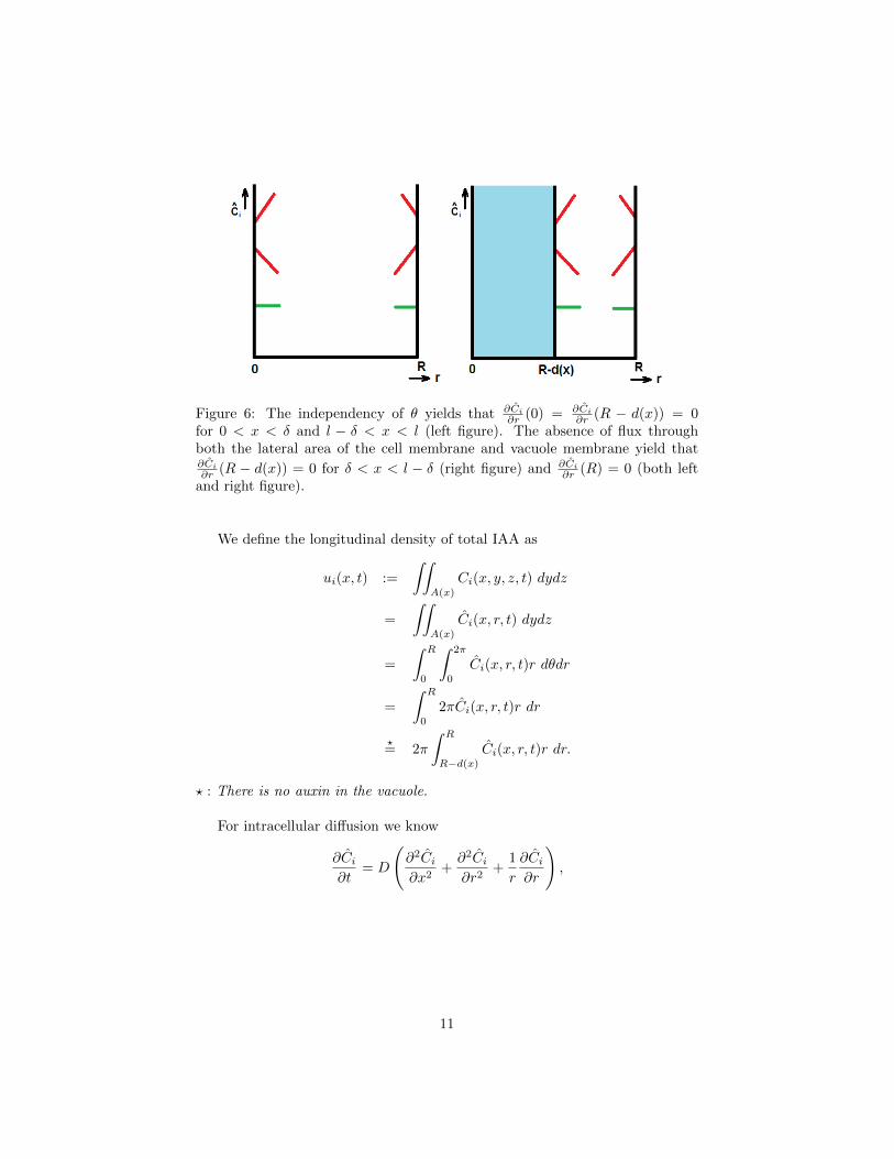
Figure 6: The independency of θ yields that ∂Ci∂r (0) = ∂Ci

∂r (R − d(x)) = 0for 0 < x < δ and l − δ < x < l (left figure). The absence of flux throughboth the lateral area of the cell membrane and vacuole membrane yield that∂Ci∂r (R − d(x)) = 0 for δ < x < l − δ (right figure) and ∂Ci

∂r (R) = 0 (both leftand right figure).

We define the longitudinal density of total IAA as

ui(x, t) :=

∫∫A(x)

Ci(x, y, z, t) dydz

=

∫∫A(x)

Ci(x, r, t) dydz

=

∫ R

0

∫ 2π

0

Ci(x, r, t)r dθdr

=

∫ R

0

2πCi(x, r, t)r dr

?= 2π

∫ R

R−d(x)

Ci(x, r, t)r dr.

? : There is no auxin in the vacuole.

For intracellular diffusion we know

∂Ci∂t

= D

(∂2Ci∂x2

+∂2Ci∂r2

+1

r

∂Ci∂r

),

11

where D is the effective diffusivity, so for intracellular diffusion we get

∂ui∂t

= 2π

∫ R

R−d(x)

∂Ci∂t

r dr

= 2π

∫ R

R−d(x)

D

(∂2Ci∂x2

+∂2Ci∂r2

+1

r

∂Ci∂r

)r dr

= 2πD

∫ R

R−d(x)

∂2Ci∂x2

r dr +

∫ R

R−d(x)

∂2Ci∂r2

r dr︸ ︷︷ ︸(&)

+

∫ R

R−d(x)

∂Ci∂r

dr

,

where

(&) =

[∂Ci∂r

r

]RR−d(x)

−∫ R

R−d(x)

∂Ci∂r

dr

(2)= −

∫ R

R−d(x)

∂Ci∂r

dr.

So

∂ui∂t

= 2πD

∫ R

R−d(x)

∂2Ci∂x2

r dr

= D∂2

∂x2

(2π

∫ R

R−d(x)

Ci(x, r, t)r dr

)

= D∂2ui∂x2

. (3)

For intracellular diffusion and active transport in longitudinal direction we know

∂Ci∂t

= D

(∂2Ci∂x2

+∂2Ci∂r2

+1

r

∂Ci∂r

)− v∇Ci,

where v is the transport velocity vector field, but we don’t know anything aboutthe v-field. There may be active transport within the cell, as there should bein large (5 cm) Chara and Nitella cells, [2, 9]. The precise mechanism thereis not yet known, nor is there particular evidence that such transport exists inthe much smaller Arabidopsis transport cells (∼ 100 µm). In order to be ableto proceed investigations, we make the simplest imaginable phenomenologicalmodification of (3) that effectively includes active transport, namely

∂ui∂t

= D∂2ui∂x2

− v ∂ui∂x

. (4)

Now we have one-dimensional equations for the auxin transport within the cellsby intracellular diffusion only and for transport within the cells for both intra-cellular diffusion and active transport.

12

4 Cell Array Models

Now we have made the necessary preparations we will proceed with modellingthe entire system. This entire system consist of an array of cells.

Figure 7: Cartoon of the experimental set-up.

4.1 Fast Homogenization within Cells

As a first and easiest approach we assume that the concentration of auxin willbe equally distributed within the cells very fast. This assumption might notbe realistic, because the transport within the cell might not be so fast that theconcentration can be considered homogeneous at all times. When you assumehomogeneity every molecule of auxin effects the concentration everywhere in thecell and so the length of the cells doesn’t play any role in the intracellular trans-port velocity when this assumption is made. However when the total number ofcells will become very large, the length of the cells will become very small. Inthis case the transport can be considered to be instantaneous, since both endsof the cells are very close to each other. This approximates a situation wherethere is fast homogenization within the cells and thus this might give some use-ful results.With the expressions of number fluxes and the assumption of fast homogeniza-tion within the cells the change of the concentration in time for each cell cannow easily be described. We get

dCidt

=Ji−1,i

V− Ji,i+1

V

=Ji−1,i − Ji,i+1

V, i ∈ {2, 3, . . . , N − 1}

dC1

dt=

Jin − J1,2

VdCNdt

=JN−1,N − Jout

V

13

where V is the volume of the cell.Substituting (1) gives us the change of concentration in time for each cell:

dCidt

=−PA(Ci −RCi−1) + PA(Ci+1 −RCi)

V, i ∈ {2, 3, . . . , N − 1}

dC1

dt=−PinA(C1 −RinCd) + PA(C2 −RC1)

VdCNdt

=−PA(CN −RCN−1) + PoutRoutACN )

V(5)

A simulation in Matlab gives the results in Figure 8. Parameter values weretaken as described in Appendix A.As you can see in Figure 8 the stem fills up very fast. This is the effect of the

Figure 8: Concentration of auxin in mol in the cells of the stem at t=20 (upperfigure), t=200 (middle figure) and t=400(bottom figure).

instantaneous transport of auxin within the cells. This is too fast to match theexperiment. We will make a continuum approximation of the cell array modelin Section 4.3.To assess the validity of the homogenization assumption, we shall consider thecase of intracellular diffusion and active transport.

14

4.2 A Model with Intracellular Diffusion and Active Trans-port

When there is no equal distribution of auxin within the cells the concentrationof the apical end of the cells can differ from the concentration on the basal endof the cell. Modifying (5) to this case gives

dCidt

=−PA(Cai −RCbi−1) + PA(Cai+1 −RCbi )

V, i ∈ {2, 3, . . . , N − 1}

dC1

dt=−PinA(Ca1 −RinCd) + PA(Ca2 −RCb1)

V

dCNdt

=−PA(CaN −RCbN−1) + PoutRoutAC

bN

V,

where Cai and Cbi are the concentrations at the apical end of the cell and thebasal end of the cell respectively.By definition we have

Ci(t) =1

V

∫ l

0

ui(x, t) dx

Cai (t) =ui(0, t)

A

Cbi (t) =ui(l, t)

A.

Within the cells we have (4). It follows that

1

V

∫ l

0

D∂2ui∂x2−v ∂ui

∂xdx =

−P (ui(0, t)−Rui−1(l, t)) + P (ui+1(0, t)−Rui(l, t))V

.

Modifying (1) to this case gives

Ji,i+1 = −P (ui+1(0)−Rui(l)), i ∈ {1, 2, . . . , N − 1}Jin = −Pin(u1(0)−RinACd)Jout = PoutRoutuN (l). (6)

We get

∂ui∂t

(0, t) = Ji−1,i −(−D∂ui

∂x(0, t) + vui(0, t)

)∂ui∂t

(l, t) = −D∂ui∂x

(0, t) + vui(0, t)− Ji,i+1.

Simulating this is not as easy as when auxin is equally distributed within thecells, because in this case we have a concatenation of partial differential equa-tions. Numerical simulation was not within the scope of this thesis. Instead weconsider the steady state solution of these these cases, that can be approachedanalytically. See Chapter 5.

15

4.3 A Continuum Approximation for fast Homogenization

With the previous derivatives we can examine how the model works with alarge number of cells in a fixed macroscopic stem length (i.e. small length of thecells). When the cells become very small the model approaches a continuum.We expect an equation of the form

∂u

∂t= D

∂2u

∂x2− v ∂u

∂x(7)

where D is the effective diffusivity constant and v the velocity.Rewriting (5) gives

dCidt

=−PA(Ci −RCi−1) + PA(Ci+1 −RCi)

V

=PA

V(RCi−1 − (1 +R)Ci + Ci+1)

=PA

V([RCi+1 − 2RCi +RCi−1] + [(1−R)Ci+1 + (R− 1)Ci])

=PAR

V∆x2

[Ci+1 − 2Ci + Ci−1

∆x2

]+PA(1−R)

V∆x

[Ci+1 − Ci

∆x

],(8)

where ∆x is the length of the cells.When N →∞ (i.e. ∆x→ 0) then, formally,

Ci+1 − 2Ci + Ci−1

∆x2→ ∂2Ci

∂x2

Ci+1 − Ci∆x

→ ∂Ci∂x

.

It follows from (7) and (8) that

D = lim∆x→0

PAR

V∆x2

and

v = lim∆x→0

PA(R− 1)

V∆x.

Assume that V = A∆x, then

D = lim∆x→0

PAR

A∆x∆x2

= lim∆x→0

PR∆x

= lim∆x→0

1

2PsPs + Pex

Ps∆x

= lim∆x→0

1

2(Ps(1− fc) + Pexfc)∆x

16

and

v = lim∆x→0

PA(R− 1)

A∆x∆x

= lim∆x→0

P (R− 1)

= lim∆x→0

1

2Ps

(Ps + Pex

Ps− 1

)= lim

∆x→0

1

2Pexfc.

When we change the length of our cells, we want that the proportions of thethickness of the membrane compared to the entire length of the cell stays thesame. Ps is the effective permeability by means of diffusion. This is dependenton the thickness of the membrane, dm, and the diffusivity constant of the mem-brane, Dm. dm is dependent on the length of the cell. In order to keep the sameproportions we have that dm = c∆x, where c is the proportion of the thicknessof the cell membrane compared to the cell length. Dm is not dependent on. Wehave Ps = CDm

dm= C Dm

c∆x , where C is the partitioning coefficient.[1]

Pex is the effective permeability by means of the PIN transporters. We havethat Pex = dm

∆t , where ∆t is the time needed to cross the membrane. Say thatthe transport speed through the PIN transporter (in the membrane) is constant,c′, then we have that ∆t = c′dm. We get that the Pex = c

c′ and so Pex is notdependent on ∆x.

It follows that

D = lim∆x→0

1

2(Ps(1− fc) + Pexfc)∆x

= lim∆x→0

1

2

(CDm

c+ Pexfc∆x

)= C

Dm

2c

and

v = lim∆x→0

1

2Pexfc

=1

2Pex.

17

5 Steady State Analysis

The system of flux-coupled diffusion-convection equations for the cell array (seeSection 4.2) is quite complicated to analyse dynamically. Instead we will deter-mine the steady state solutions for diffusion within the cells and for diffusionand active transport within the cells. Then the number flux between adjacentcells is equal for every two adjacent cells. The number flux from the donor wellinto the stem and from the stem into the receiver well are also equal to thisnumber flux between adjacent cells.Recall that in our model we assume that there is no diffusion of auxin in radialtransversal direction out of the transport channel.

5.1 Case of Intracellular Diffusion

We investigate the assumption of diffusion by examining the steady state solu-tion of our model.When the system is in steady state the number flux between adjacent cells andthe number flux into the stem and out of the stem must be equal to each other.In the case of steady state we have

J := J0,1 = Ji,i+1 = JN,N+1,

for all i.Let u?i (x) be the steady state solution, then we get from (1), with l the celllength,

J = −PA(u?i+1(0)

A−Ru

?i (l)

A

), i ∈ {1, 2, . . . , N − 1}

= −P (u?i+1(0)−Ru?i (l))

J = −PinA(u?1(0)

A−RinCd

)= −Pin(u?1(0)−RinACd)

J = PoutRoutAu?N (l)

A= PoutRoutu

?N (l) (9)

Within the cell the diffusion equation applies, so we know

∂ui∂t

= D∂2u

∂x2,

where D is the effective diffusivity of auxin within the cells and thus

∂2u?i∂x2

= 0.

It follows that the steady state solution has the form

u?i (x) = c1 + c2x. (10)

18

It’s easy to see that c1 = u?i (0) and c2 =∂u?i∂x . From Fick’s first law of diffusion

we know that the diffusive flux inside cell i equals −D ∂u?i∂x . Since the system is

in steady state it must hold that

J = −D∂u?i

∂x= −Dc2

and hence

c2 = − JD.

Substitution into (10) gives

u?i (x) = u?i (0)− J

Dx

as the steady state solution for cell i.

From (9) we get that

u?1(0) = − J

Pin+RinACd,

u?i+1(0) = − JP

+Ru?i (l)

= − JP

+R

(u?i (0)− Jl

D

)= −J

(1

P+R

l

D

)+Ru?i (0). (11)

Let xi = u?i (0) and let x1 = u?1(0), then

xi+1 = αxi + β,

x1 = γ, (12)

where α = R, β = −J(

1P +R l

D

)and γ = − J

Pin+RinACd.

From this follows:

x2 = αγ + β

x3 = α(αγ + β) + β

= α2γ + αβ + β

x4 = α(α2γ + αβ + β) + β

= α3γ + α2β + αβ + β

Now it’s easy to see that

xn = αn−1γ + β

(n−2∑k=0

αk

)

=

{γ + β(n− 1), α = 1

αn−1γ + β αn−1−1α−1 , α 6= 1

. (13)

19

Replacing the xn, α, γ and β gives

u?n(0)R 6=1= Rn−1

(− J

Pin+RinACd

)− J

(1

P+R

l

D

)Rn−1 − 1

R− 1. (14)

From (9) we get that

u?N (l) =J

PoutRout− ACrRout

Cr=0=

J

PoutRout,

u?N (0) =J

PoutRout+Jl

D

= J

(1

PoutRout+

l

D

).

From (14) we get that

u?N (0) = RN−1

(− J

Pin+RinACd

)− J

(1

P+R

l

D

)RN−1 − 1

R− 1.

It follows that

J

(1

PoutRout+

l

D

)= RN−1

(− J

Pin+RinACd

)−J

(1

P+R

l

D

)RN−1 − 1

R− 1,

RN−1RinACd = J

(1

PoutRout+

l

D+RN−1

Pin

+

(1

P+R

l

D

)RN−1 − 1

R− 1

).

20

J = RN−1RinACd ·[

1

PoutRout+

l

D+RN−1

Pin

+1

P

RN−1 − 1

R− 1+

l

D

RN −RR− 1

]−1

= RinACd ·[

1

PoutRoutRN−1+

l

D

1

RN−1+

1

Pin

+1

P

1− 1RN−1

R− 1+

l

D

R− 1RN−2

R− 1

]−1

= RinACdD

l·

[(1 +

Dl

PoutRout

)1

RN−1+

Dl

Pin

+Dl

P

1

R− 1

(1− 1

RN−1

)+

R

R− 1

(1− 1

RN−1

)]−1

= RinACdD

l·

[(1 +

Dl

PoutRout

)1

RN−1

+

(R

R− 1+

Dl

Pin+

Dl

P

1

R− 1

)(1− 1

RN−1

)+

Dl

Pin

1

RN−1

]−1

= RinACdD

l·

[(1 +

Dl

PoutRout+

Dl

Pin

)1

RN−1

+

(R

R− 1+

Dl

Pin+

Dl

P

1

R− 1

)(1− 1

RN−1

)]−1

N large≈ RinACd

D

l

[R

R− 1+

Dl

Pin+

Dl

P

1

R− 1

]−1

= RinACdD

l

(1− 1

R

)[1 +

Dl

Pin

(1− 1

R

)+

Dl

P

1

R

]−1

.

Filling in our parameter values, putting R = 100, gives

J ≈ 9× 10−18 mol/s, for Pin = 1× 10−7 m/s

andJ ≈ 4× 10−17 mol/s, for Pin = 7× 10−7 m/s.

With experiments is measured that J ≈ 9× 10−18 mol/s (see Figure 2 on page5). So for Pin ∼ 1 × 10−7 m/s we get a value for J that fits the experimentalresults. In Section 5.4 and Appendix C equation (13) is further examined. Weknow that for α� 1 the profile is likely to blow up for small n. In this case wehave α = R� 1 so we expect this profile to blow up, but maybe ε = (α−1)γ+βis small enough.

21

Filling in our parameter values and taking J = 9 × 10−18 mol/s and Pin =1× 10−7 m/s gives

α = 100,

β ≈ −1× 10−9 mol/m,

γ = 1× 10−11 mol/m

and

ε ≈ −1× 10−10 mol/m.

Taking J = 4× 10−17 mol/s and Pin = 7× 10−7 m/s gives

α = 100,

β = −5× 10−9 mol/m,

γ ≈ 4× 10−11 mol/m

and

ε ≈ −1× 10−10 mol/m.

For both Pin = 1× 10−7 m/s and Pin = 7× 10−7 m/s we get ε < 0. AppendixC shows that for ε < 0 the profile doesn’t relate to the experimental results.As mentioned, see Section 5.4 for further analysis.

5.2 Case of Intracellular Diffusion and Transport

We also take a look at a model with active transport within the cells. In Charaand Nitella cells their is evidence that such transport should exist because of thesize of these cells, although its biochemical/-physical origins are unclear, [2, 9].As we did before in the previous section we can determine the steady statesolution. With active transport within cells we have the following governingequations:

∂ui∂t

= D∂2ui∂x2

− v ∂ui∂x

Here v is the transport velocity within the cells.So for the steady state solution u?i it follows that

D∂2u?i∂x2

− v ∂u?i

∂x= 0

and hence our steady state solution has the form

u?i (x) = c1 + c2evD x, v 6= 0. (15)

The number flux at point x within cell i in the direction of increasing x is

−D∂u?i

∂x+ vu?i (x).

22

Obviously in steady state the number fluxes between cells has to keep up withthis flow in the cells. We get

J = −D∂u?i

∂x+ vu?i (x)

= −D[c2v

DevD x]

+ v(c1 + c2e

vD x)

= −c2vevD x + c1v + c2ve

vD x

= c1v.

So

c1 =J

v.

Substituting this in (15) gives

u?i (x) =J

v+ c2e

vD x

u?i (0) =J

v+ c2

c2 = u?i (0)− J

v

u?i (x) =J

v+

(u?i (0)− J

v

)evD x

=J

v

(1− e vD x

)+ u?i (0)e

vD x.

From (9) we get

u?1(0) = − J

Pin+RinACd

u?i+1(0) = − JP

+Ru?i (l)

= − JP

+R

(J

v

(1− e vD l

)+ u?i (0)e

vD l

)= − J

P+R

J

v

(1− e vD l

)+Re

vD lu?i (0).

We have the same form as before, see (12), where now α = RevD l, β = − J

P +

RJv

(1− e vD l

)and γ = − J

Pin+RinACd.

From (13) we get

u?N (0) = RN−1e(N−1) vD l

(− J

Pin+RinACd

)+

(− JP

+RJ

v

(1− e vD l

)) RN−1e(N−1) vD l − 1

RevD l − 1

.

23

From (9) we also have

u?N (l) =J

PoutRoutJ

v

(1− e vD l

)+ u?N (0)e

vD l =

J

PoutRout

u?N (0) =J(

1PoutRout

− 1v

(1− e vD l

))evD l

.

It follows that

J(

1PoutRout

− 1v

(1− e vD l

))evD l

= RN−1e(N−1) vD l

(− J

Pin+RinACd

)+

(− JP

+RJ

v(1− e vD l)

)·R

N−1e(N−1) vD l − 1

RevD l − 1

z = evD l

J(

1PoutRout

− 1v (1− z)

)z

= RN−1zN−1

(− J

Pin+RinACd

)+

(− JP

+RJ

v(1− z)

)RN−1zN−1 − 1

Rz − 1

y = Rz

J(

1PoutRout

− 1v

(1− y

R

))yR

= yN−1

(− J

Pin+RinACd

)+

(− JP

+RJ

v

(1− y

R

)) yN−1 − 1

y − 1

J(

1PoutRout

− 1v

(1− y

R

))yN

R

= − J

Pin+RinACd

+

(− JP

+RJ

v

(1− y

R

)) 1− 1yN−1

y − 1

24

RinACd = J

(1

Pin+

(1

P−R1

v

(1− y

R

)) 1− 1yN−1

y − 1

+1

PoutRout− 1

v

(1− y

R

)yN

R

)

= J

(1

Pin− 1

v

(R− y − v

P

) 1− 1yN−1

y − 1+

R

yN1

PoutRout

−RyN− 1

yN−1

v

)

J = RinACd

[1

Pin− 1

v

(R− y − v

P

) 1− 1yN−1

y − 1+

R

yN1

PoutRout

−RyN− 1

yN−1

v

]−1

N large≈ RinACd

[1

Pin− 1

v

(R− y − v

P

) 1

y − 1

]−1

= RinACd

[1

Pin+

(1

P− R

v(1− e vD l)

)1

RevD l − 1

]−1

.

Since the value for v is unknown we use J = 9 × 10−18 mol/s from the ex-perimental results to determine a value for v. Filling in our parameter valuesgives

v ≈ 2× 10−7 m/s, for Pin = 1× 10−7 m/s

v ≈ −3× 10−6 m/s, for Pin = 7× 10−7 m/s.

Since v < 0 for Pin = 7× 10−7 m/s, only Pin = 1× 10−7 m/s will be examinedfurther.Taking J = 9× 10−18 mol/s and v = 2, 13903× 10−7 m/s we get

α = 100 · e2×10−1

,

β ≈ −1× 10−9 mol/m,

γ = 1× 10−11 mol/m

and

ε ≈ −7× 10−11 mol/m.

Note that J is dependent on v, so v = 2, 13903 m/s is not the exact value toget J = 9× 10−18 mol/s.Again we have ε < 0 and Appendix C shows that the profile doesn’t relate tothe experimental results when ε < 0.

25

5.3 Case of Intracellular Mixing

Another possibility is the case of intracellular mixing. This case yields that theauxin is equally distributed within each cell when the system is in steady state.We get

u?i (x) = u?i (0).

From (9) we get that

u?1(0) = − J

Pin+RinACd

u?i+1(0) = − JP

+Ru?i (l)

= − JP

+Ru?i (0)

Again we have the same form as in (12). As with diffusion we have α = R andγ = − J

Pin+RinACd. In this case we have β = − J

P . From (13) we get

u?N (0) = RN−1

(− J

Pin+RinACd

)− J

P

RN−1 − 1

R− 1.

From (9) we also have

u?N (l) =J

PoutRout

u?N (0) =J

PoutRout

It follows that

J

PoutRout= RN−1

(− J

Pin+RinACd

)− J

P

RN−1 − 1

R− 1

RN−1RinACd = J

(1

PoutRout+RN−1

Pin+

1

P

RN−1 − 1

R− 1

)RinACd = J

(1

PoutRoutRN−1+

1

Pin+

1

P

1− 1RN−1

R− 1

)

J = RinACd ·[(

1

PoutRout+

1

Pin

)1

RN−1+

(1

Pin+

1

P

1

R− 1

)(1− 1

RN−1

)]−1

N large≈ RinACd ·

[1

Pin+

1

P

1

R− 1

]−1

> 0

Filling in our parameter values gives

J ≈ 1× 10−17 mol/s, for Pin = 1× 10−7 m/s

26

andJ ≈ 6× 10−17 mol/s, for Pin = 7× 10−7 m/s.

For Pin = 1×10−7 m/s we have a value for J that fits the experimental results.Filling in our parameter values and taking J = 1 × 10−17 mol/s and Pin =1× 10−7 m/s gives

α = 100

β ≈ −3× 10−10 mol/m

γ = 0 mol/m

and

ε ≈ −3× 10−10 mol/m.

Taking J = 6× 10−17 mol/s and Pin = 7× 10−7 m/s gives

α = 100

β ≈ −2× 10−9 mol/m

γ ≈ 1× 10−11 mol/m

and

ε ≈ −9× 10−11 mol/m.

We get ε < 0 for both Pin = 1×10−7 m/s and Pin = 7×10−7 m/s. This doesn’trelate to the experimental results.

5.4 Examining Exponential ’Blow-up’ in Detail

From the previous sections it becomes clear that to assess the profile found withthe experiments a more detailed analysis is needed than that exhibited in Ap-pendix C. Such an analysis is also needed to be able to draw strong conclusionson the validity of the proposed models. In this section a less sensitive approachis used instead.Recall that for intracellular diffusion and transport we have

α = RelD v,

β = −J

(1

P−R1− e l

D v

v

),

and

γ = u?1(0) = − J

Pin+RinACd.

27

Define

β :=β

u?1(0)

=−J

(1P −R

1−evDl

v

)− JPin

+RinACd

=−PinP

PinRinACdJ − 1

·[1− PR1− e vD l

v

],

then

u?n(0)

u?1(0)=

{αn−1 + β α

n−1−1α−1 , α 6= 1

1 + β(n− 1), α = 1

=

{αn−1

(1 + β

α−1

)− β

α−1 , α 6= 1

1 + β(n− 1), α = 1.

Recall

u?N (l) =

(u?N (0)− J

v

)elD v +

J

v

and define

λ :=l

Dv,

then

u?N (l) =

(αN−1

(u?1(0) +

β

α− 1

)− β

α− 1− J

v

)eλ +

J

v

= eλ(αN−1

(u?1(0) +

β

α− 1

)− β

α− 1

)+J

v(1− eλ)

Recall

u?N (l) =J

PoutRout.

We get

J

PoutRout= eλ

(αN−1

(u?1(0) +

β

α− 1

)− β

α− 1

)+J

v(1− eλ)

J

(1

PoutRout− 1− eλ

v

)= eλ

(αN−1

(u?1(0) +

β

α− 1

)− β

α− 1

)

J

(1

PoutRout− 1− eλ

v+ eλ

(αN−1

α− 1

(1

P−R1− eλ

v

)− 1

α− 1

(1

P−R1− eλ

v

)))= eλαN−1u?1(0)

J

(1

PoutRout− 1− eλ

v+ eλ

(αN−1 − 1

α− 1

(1

P−R1− eλ

v

)))= eλαN−1u?1(0)

28

J

u?1(0)=

eλαN−1

1PoutRout

− 1−eλv + eλ

(αN−1−1α−1

(1P −R

1−eλv

)) (16)

Then

β =β

u?1(0)

=−J

(1P −R

1−eλv

)u?1(0)

(16)= − eλαN−1

1PoutRout

− 1−eλv + eλ

(αN−1−1α−1

(1P −R

1−eλv

)) · ( 1

P−R1− eλ

v

).

Put

δ :=1

P−R1− eλ

v,

then

β

α− 1= − eλαN−1δ

(α− 1)(

1PoutRout

− 1−eλv

)+ eλ(αN−1 − 1)δ

= − 1

α−N+1 α−1δ e−λ

(1

PoutRout− 1−eλ

v

)+ 1− α−N+1

Recall

u?N (0) = αN−1u?1(0)− βαN−1 − 1

α− 1.

It follows that

u?N (0)

u?1(0)= αN−1 + β

αN−1 − 1

α− 1

= αN−1

(1 +

β

α− 1

)− β

α− 1

= αN−1

α−N+1 α−1δ e−λ

(1

PoutRout− 1−eλ

v

)− α−N+1

α−N+1 α−1δ e−λ

(1

PoutRout− 1−eλ

v

)+ 1− α−N+1

− β

α− 1

=

α−1δ e−λ

(1

PoutRout− 1−e−λ

v

)− 1

α−N+1 α−1δ e−λ

(1

PoutRout− 1−eλ

v

)+ 1− α−N+1

− β

α− 1

=

α−1δ e−λ

(1

PoutRout− 1−e−λ

v

)α−N+1 α−1

δ e−λ(

1PoutRout

− 1−eλv

)+ 1− α−N+1

.

29

Define

ρ :=α− 1

δe−λ

(1

PoutRout− 1− e−λ

v

),

then

u?N (0)

u?1(0)=

ρ

α−N+1(ρ− 1) + 1

=ρ

ρ−1αN−1 + 1

≈ ρ. (17)

For 1 ≤ n ≤ N it holds that

u?n(0)

u?1(0)=

αn−Nρ− αn−N + 1

α−N+1(ρ− 1) + 1

=αn−N (ρ− 1) + 1

ρ−1αN−1 + 1

≈ αn−N (ρ− 1) + 1. (18)

For the diffusive case, i.e. v = 0, we get

ρ = limv→0

α− 1

δe−

lD v

(1

PoutRout− 1− e− l

D v

v

)

=α− 1

δ

(1

PoutRout+

l

D

),

δ = limv→0

1

P−R1− e l

D v

v

=1

P+R

l

D

and

α = limv→0

RelD v

= R.

30

So for the diffusive case it follows that

ρ =R− 1

1P +R l

D

(1

PoutRout+

l

D

)=

1PoutRout

+ lD

1P (R−1) + R

R−1lD

=D

l·PoutRout + 1Dl

P (R−1) + RR−1

=D

l·PoutRout + 1Dl

P (R−1) + 1R−1 + 1

=D

l·PoutRout + 1Dl +P

P (R−1) + 1.

With our parameter values, putting R = 101 we get

ρ ≈ 40.

Also α = 101 and N = 160, so

αN−1 = 101159.

This is big enough for (17) and (18) to be good approximations, so

u?N ≈ 40u?1(0).

It also gives us the following profile:

u?n(0)

u?1(0)= 1 +

ρ− 1

αN−n

For the last cell we get ρ = 40.For the second last we get 1 + ρ−1

α = 1 + 39101 ≈ 1.386.

For the third last we get 1 + ρ−1α2 = 1 + 39

10201 ≈ 1.004.Note that in comparison with the last cell all the other values are close to 1. Sothis gives us a pretty flat profile with a very small peak at the very end.

31

6 Discussion and Conclusions

This thesis examined the transport of auxin in Arabidopsis thaliana. The start-ing point was the article of G.J. Mitchison, [8]. This article suggested that therewas simple diffusion within cells as only form of transport within the cells ofArabidopsis. There was some reasonable doubt whether this is true or not.In this thesis there is some support. The value found for the flux of auxin be-tween adjacent cells, assuming simple diffusion, corresponds to the value mea-sured with experiments done in the Plant BioDynamics Laboratory in Leiden.However in other cases this value also corresponds to the experiments.Assuming simple diffusion also gave us a reasonably good match with the pro-file of the distribution of auxin within the stem. Other cases in this thesis arenot examined and it can be that something other than simple diffusion gives amatch as well as this one.The formula for the profile as used in Appendix C should be used carefully ornot at all in further investigation. The approach in Section 5.4 is recommendedto be used instead.

32

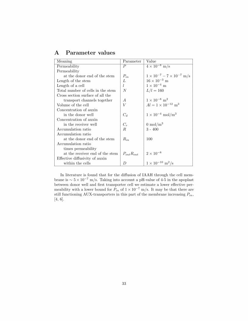
A Parameter values

Meaning Parameter ValuePermeability P 4× 10−8 m/sPermeability

at the donor end of the stem Pin 1× 10−7 − 7× 10−7 m/sLength of the stem L 16× 10−3 mLength of a cell l 1× 10−4 mTotal number of cells in the stem N L/l = 160Cross section surface of all the

transport channels together A 1× 10−8 m2

Volume of the cell V Al = 1× 10−12 m3

Concentration of auxinin the donor well Cd 1× 10−4 mol/m3

Concentration of auxinin the receiver well Cr 0 mol/m3

Accumulation ratio R 3 - 400Accumulation ratio

at the donor end of the stem Rin 100Accumulation ratio

times permeabilityat the receiver end of the stem PoutRout 2× 10−8

Effective diffusivity of auxinwithin the cells D 1× 10−10 m2/s

In literature is found that for the diffusion of IAAH through the cell mem-brane is ∼ 5× 10−7 m/s. Taking into account a pH-value of 4-5 in the apoplastbetween donor well and first transporter cell we estimate a lower effective per-meability with a lower bound for Pin of 1× 10−7 m/s. It may be that there arestill functioning AUX-transporters in this part of the membrane increasing Pin,[4, 6].

33

B Matlab Simulation

B.1 Parameters.m

L=16*10^-3; % length of the stem in m

N=160; % number of cells

l=L/N; % length of cells in m

d=25*10^-6; % diameter cell in m

fu=0.15; % fraction non-vacuole

fa=0.5; % fraction auxin in anion form in apoplast

fc=0.97; % fraction auxin in anion form in cell (cytoplasm)

fd=0.97; % fraction auxin in anion form in donor well

Cd=1*10^-4; % concentration donor well (mol/m^3)

Cr=0; % concentration receiver well

Ps=5*10^-7; % permeability for diffusion protonated form

Pex=5*10^-6*fc; % transporters

P=Ps*(1-fc)/2; % permeability

Pin=Ps*(1-fd)/2; %

Pout=Ps*(1-fc)/2; %

A=pi*(d/2)^2; % cross surface between cells in m^2

V=A*l*fu; % volume cell in m^3

R=1+Pex*fc/(Ps*(1-fc)); % accumulation ratio

Rin=1+Pex*fd/(Ps*(1-fd));

Rout=1+Pex*fc/(Ps*(1-fc));

N=round(N); % rounding N to an integer value

D=10^-10; % diffusion constant auxin in cell in m^2/s

Pr=2.4*10^-8; % Pout*Rout

B.2 conc.m

function dy = conc(t,y,P,Pin,Pout,A,V,R,Rin,Rout,Cd,Cr,N)

dy = zeros(N,1);

dy(1) = (-Pin*A*(y(1)-Rin*Cd)+P*A*(y(2)-R*y(1)))/V;

for i=2:N-1

dy(i) = (-P*A*(y(i)-R*y(i-1))+P*A*(y(i+1)-R*y(i)))/V;

end

dy(N) = (-P*A*(y(N)-R*y(N-1))+Pout*A*(Cr-Rout*y(N)))/V;

34

B.3 Auxplot.m

[T,Y] = ode45(@(t,y)conc(t,y,P,Pin,Pout,A,V,R,Rin,Rout,Cd,Cr,N),[0 10^5],zeros(N,1));

X = zeros(N,1);

for i = 1:N

X(i) = i;

end

YT = Y’;

hold off

bar(X,YT(:,21)) % The integer in this line is the value for t+1

35

C Examining equation (13)

Now we examine the profile of xn (as a function of n) for different α, β and γin

xn =

{γ + β(n− 1), α = 1

αn−1γ + β αn−1−1α−1 , α 6= 1

. (19)

We know that α, γ > 0 and β < 0. Considering we don’t want xn to blow upfast we can distinguish between α = 1 and α > 1. α < 1 is not relevant becausewe need an increase in the profile of xn.When α = 1 we get

xn = γ + (n− 1)β,

so the profile of xn is a straight line with a slope of β starting at γ. Concentra-tions of auxin will be negative if n is large enough.

When α > 1 and β = 0 we get that the profile is exponentially increasing, butβ < 0, so β can cancel out the increase. When we have β such that x2 = x1 = γ,we get from (19) that

γ = αγ + β

β = −(α− 1)γ.

When we substitute this back into (19) we get

xn = αn−1γ − (α− 1)γαn−1 − 1

α− 1

= αn−1γ −(αn−1 − 1

)γ

= γ.

So when α > 1 and β = −(α− 1)γ we get that the profile of xn is constant.

36

Take β = −(α− 1)γ + ε, where ε 6= 0, and let α > 1, then we get from (19)that

xn = αn−1γ − ((α− 1)γ − ε) αn−1 − 1

α− 1

= αn−1γ − (α− 1)γαn−1 − 1

α− 1+ ε

αn−1 − 1

α− 1

= γ + εαn−1 − 1

α− 1.

Define

x(ν) := γ + εαν

α− 1, ν > 0

where ν = n − 1 is a continuous variable. Looking at the first and secondderivative of x(ν),

dx

dν= ε

αν log(α)

α− 1

d2x

dν2= ε

αν log2(α)

α− 1,

we see that for α > 1 the sign of the first and second derivative is that of ε.So when α > 1 and ε > 0 we get that x(ν) has an increasing and convex expo-nential profile. when α > 1 and ε < 0 we get that x(ν) has a decreasing andconcave exponential profile.

37

In the case of ε > 0 we have a profile that relates to the experimental results.In the first derivative of x(ν) we can see that the slope is determined by α and ε.When α & 1 the profile will blow op when ν is large enough. When α� 1 theprofile will blow up for small ν. When ε increase, the slope of x(ν) increases.So when ε & 0 it can compensate a blow up that could appear when α� 1.

38

References

[1] Theo Blom, Transport and Accumulation of Alkaloids in Plant Cells, PhDthesis Rijksuniversiteit Leiden, pp. 42, 1991.

[2] Kees Boot, Kees Libbenga, Sander Hille, Remko Offringa and Bert vanDuijn, Polar Auxin Transport: an Early Invention, Journal of ExperimentalBotany, Vol. 63, No. 11, pp. 4213-4218, 2012.

[3] A. Chavarria-Krauser and M. Ptashnyk, Homogenization of Long RangeAuxin Transport in Plant Tissue, Nonlinear Analysis: Real World Appli-cations, Vol. 11, No. 6, pp. 4524-4532, 2010.

[4] A. Delbarre, P. Muller, V. Imhoff and J. Guern, Comparison of MechanismsControlling Uptake and Accumulation of 2,4-dichlorophenoxy Acetic Acid,Naphthalene-1-acetic Acid, and Indole-3-acetic Acid in Suspension-culturedTobacco Cells, Plante, Vol. 198, No. 4, pp. 532-541, 1996.

[5] E.M. Kramer, A Mathematical Model of Pattern Formation in the VascularCambium of Trees, Journal of Theoretical Biology, Vol. 216, No. 2, pp. 147-158, 2002.

[6] E.M. Kramer, How Far Can a Molecule of Weak Acid Travel in the Apoplastor Xylem?, Plant Physiology, Vol. 141, No. 4, pp. 1233-1236, 2006.

[7] Ottoline Leyser, Auxin, Current Biology, Vol. 11, No. 18, pp. R728, 2001.

[8] G.J. Mitchison, The Dynamics of Auxin Transport, Proc. R. Soc. Lond. B,No. 209, pp. 489-511, 1980.

[9] J.A. Raven, Polar Auxin Transport in Relation to Long-distance Transportof Nutrients in the Charales, Journal of Experimental Botany, Vol. 64, No.1, pp. 1-9, 2013.

39