Photometry of Outer-belt Objectsby

Gautham S. Narayan

Submitted to the Department of Physicsin partial fulfillment of the requirements for Research Honors

at

Illinois Wesleyan University

April 2005

© Gautham S. Narayan, 2005. All rights reserved.

The author hereby grants to Illinois Wesleyan University permission to reproduce anddistribute publicly paper and electronic copies of this thesis document in whole or in part,

and to grant others the right to do so.

Author:Department of Physics

Certified by:Dr. Linda M. French

Reader

Certified by:Dr. Narendra K. Jaggi

Reader

Certified by:Dr. Ram S. Mohan

Reader

Certified by:Dr. Gabriel C. Spalding

Reader

CONTENTS

Abstract ... 11. Introduction ... 22. Instrumentation and Observations

2.1 The Optical Path and Measurement Chain ... 52.2 Auxiliary Hardware ... 72.3 Observed Objects and Observing Procedure ... 82.4 Bias and Readout Noise in Observations ... 82.5 Non-uniform Detector Response and Flat-fields ... 92.6 The Real Time Display and On-site Analysis ..112.7 Observing Landolt Standard Stars ..122.8 Observing Outer-belt Objects – Telescope Tracking Rates and Airmass .122.9 End of Observing Procedures ..13

3. Image Reduction3.1 Overscan Correction and Trimming ..143.2 Bias Correction ..153.3 Flat-fielding ..16

4. Photometry4.1 Centroid Determination, Background Removal & Aperture Photometry .184.2 Determining Coefficients of the Transformation Equations ..204.3 Determining Magnitudes from the Johnson-Kron-Cousins system ..254.4 Determining Absolute Magnitudes ..27

5. Analysis and Results5.1 Period Determination Using Phase Dispersion Minimization ..295.2 The Magnitude Equation and Size Ratios ..305.3 Results ..315.4 Results for 279 Thule ..315.5 Results for C/2002 CE10 (LINEAR) ..36

6. Acknowledgements ..37References ..38Appendix A:

A.1 The Magnitude Equation ..40A.2 The Point Spread Function ..41A.3 Atmospheric Extinction and Transformation Equations ..43

Appendix B:B.1 Charge Coupled Devices ..46B.2 Quantum Efficiency of our CCD, and Filter Transmission Curves ..47

ABSTRACT

We present results from multi-wavelength observations of outer-belt asteroid 279 Thuleand comet C/2002 CE10 (LINEAR). The orbital elements of the second object, formerlyclassified as asteroid 2002 CE10, at first led to its identification with a group of asteroidscalled the Damocloids. The Damocloids’ orbits are similar to Halley family comets(HFCs), and there is suspicion that the Damocloids are inactive HFC nuclei. Followingobservations by the 8.2 m Japanese Subaru telescope in August 2003, which determinedthat 2002 CE10 had a characteristic tail (Takato et al; 2003), it was re-classified as cometC/2002 CE10 (LINEAR).

We observed these and other objects with filters close to the Johnson-Kron-CousinsBVRI filters corresponding to the blue, visible, red, and near-IR wavelengths using the0.9m SMARTS telescope at Cerro-Tololo Inter-American Observatory during October2003. Using the image reduction routines (imred) of the Image Reduction and AnalysisFacility (NOAO X11/IRAF), we removed the bias caused by dark currents, and flatfielded the data to improve the signal-to-noise ratio (SNR).

Instrumental magnitudes for all objects were extracted using the aperture photometrypackage (apphot). Landolt standard stars were used to solve the transformation equationsand extract extinction coefficients. Photometric calibration routines (photcal) allowed usto use the extinction coefficients and instrumental magnitudes to determine magnitudes inthe Landolt standard system. We computed absolute magnitudes for 279 Thule andC/2002 CE10 (LINEAR) in the VR bands by correcting for the changing geocentricdistance, heliocentric distance, and solar phase of the object. 279 Thule was found tohave a mean absolute visual magnitude of 8.660.01 and a V-R color of 0.440.03, whencorrected for solar phase using the standard IAU phase relation (Bowell et al; 1989). Wediscuss the suitability of the standard phase relation for 279 Thule. We place constraintson the size of the objects. We determine the rotation period for 279 Thule to be 7.60.5hrs, using an implementation of the phase dispersion minimization (PDM) algorithm firstdeveloped by Stellingwerf (1978). It is likely that observations of C/2002 CE10 (LINEAR)have been contaminated by near nucleus coma.

1

1. INTRODUCTION

Outer-belt asteroids are small objects left over from the material that accreted into theplanets. Since they presently have a low frequency of collisions, the surface compositionsof several primitive asteroids may be representative of the composition of the early solarnebula. Some asteroids are more thermally evolved because of their proximity to the sun,and may be able to shed light on early solar system processes.

Comet nuclei are especially interesting since they are likely carriers of material capturedin the sun’s proto-planetary disk some 4.5 billion years ago. However, their small sizesmake them very difficult to study, as their nuclei do not scatter many photons. As theyapproach the sun, comets develop a coma around their nucleus, which can swamp thesignal from it, making its properties very hard to determine. When they are further awayfrom the sun, they are not bright enough for photometric purposes. Thus, very fewcometary nuclei have been studied using ground-based observations. Ground-basedstudies concentrate on cometary nuclei with low out-gassing even near perihelion, such asP/Encke (Fernandez et al; 2000).

Here we present results from Johnson-Kron-Cousins BVRI observations of two outer-beltobjects, Asteroid 279 Thule and Comet C/2002 CE10 (LINEAR). A table of orbitalelements for the two objects is given below.

TABLE 1.1: ORBITAL ELEMENTS OF OBSERVED OBJECTS

(Source: Minor Planet Center, IAU)

Name a (AU) e i (deg) q (AU) P (years)

279 Thule 4.277 0.012 2.338 4.224 8.84

C/2002 CE10 (LINEAR) 9.81 0.7914 145.45 2.04 30.8

Zappala et al. (1989) have determined a rotation period of 7.44 hrs for 279 Thule.Spectroscopic observations have determined that it is a D-type asteroid (Fitzsimmons etal; 1990). Further, the same study found that 279 Thule exhibited interesting features inthe absorption spectra at 416, 441 and 515 nm that do not correspond to any knownasteroidal absorption features or known atmospheric absorption bands (Lagerkvist et al;1990). D-type asteroids appear to be redder than most outer-belt asteroids and are thoughtto be more primitive than any known meteorite; their unusual redness is thought to beevidence that their surfaces are composed of “supercarbonaceous” chondrites (Vilas et al;1985) and have not been subject to considerable heating. 279 Thule is also the onlyasteroid in a 4:3 orbital resonance with Jupiter.

2

a = semi-major axis e = eccentricity i= inclination q = perihelion distance P = orbital period

C/2002 CE10 LINEAR was discovered in February 2002 (McNaught et al; 2002).Classified as an asteroid until observations in August 2003 by the 8.2 m Japanese Subarutelescope that determined that it had a characteristic tail (Takato et al; 2003), C/2002 CE10

(LINEAR) is especially interesting as its orbital elements are similar to those of Halleyfamily comets (HFCs) and the Damocloid family of asteroids. The similarity betweenHFC and the Damocloid distribution of eccentricity and inclination suggest that theDamocloids are inactive Halley family comet nuclei (Asher et al; 1994). In addition, thedistribution of inclinations of HFCs and the Damocloids (see Fig. 1.1) is clearly distinctfrom that of Jupiter family comets (JFCs) (Jewitt, 2005) and numerical simulationsindicate that Damocloids are unlikely to be former JFCs whose orbits have evolved intoorbits that resemble HFCs (Levinson and Duncan, 1997). The theory that Damocloids aredead HFC nuclei is supported by the observations of C/2002 CE10 (LINEAR) andobservations of C/2001 OG108 (LONEOS) (Abell et al; 2005), C/2002 VQ94 (LINEAR)(Jewitt, 2005) and 2060 Chiron (Meech et al; 1989). These objects were initiallyclassified as Damocloids and were later observed exhibiting cometary activity.

3

Figure 1.1: Cumulative distributions of inclinations of various outer-belt families. The Damocloid sample(solid line) consists of 20 objects with TJ 2 and is very similar to the HFC sample (dashed line) that consistsof 42 comets with TJ 2, and periods over 200 years. The JFC sample (dashed-dotted line) consists of 240comets with 2 TJ 3, and does not appear to be related to the HFCs or Damocloids. (Source: Jewitt, 2005)

The Tisserand parameter, introduced in the late 19th century by the French mathematicianFelix Tisserand in his classic work “Traité de mécanique céleste”, can be used todistinguish between different outer-belt groups. ‘TJ’ relative to Jupiter, is defined as

TJ =aJa

+ 2 Hcos iL $%%%%%%%%%%%%%%%%%%%%%%%%%H1 - e2L aaJ

where ‘a’ is the semi-major axis and, ‘e’ is the eccentricity and ‘i’ is the inclination ofthe orbit. The semi-major axis of Jupiter ‘aJ’ is 5.2 AU. This definition assumes thatJupiter is in a circular orbit, and ignores the gravitational effects of other planets, whichhave long-term effects. However, as the Tisserand parameter depends only on semi-majoraxis, eccentricity and inclination it can be treated as a constant for an outer-belt object.HFCs and Damocloids both have TJ 2, while JFCs exhibit 2 TJ 3. Most asteroidshave TJ > 3; the Tisserand parameter clearly reflects the distinctions between the differentgroups.

Broadband photometry is a versatile tool that can be used to determine asteroid rotationperiods, constrain shape, and determine surface colors, thus contributing to anunderstanding of asteroid surface chemical composition. It is possible to use photometryeven when luminosities are insufficient to do spectroscopy or spectrophotometry, andtherefore with relatively small aperture telescopes. Outer-belt objects are generally notspherically symmetric, and they have angular momentum about an internal axis;therefore, the area they present to the earth and the amount of sunlight they reflect variesperiodically with time. By determining its absolute magnitude at different times, we canfind the rotation period of the asteroid, provided we have sufficient phase coverage.Using the magnitude variation of the lightcurve, we can place limits on the ratio of thediameters of the area the object presents towards us. In addition, if radar observations arepresent or assumptions about the fraction of the light reflected (or albedo) are made, wecan place limits on the lengths of these diameters.

The magnitude equation and other photometric terms are discussed in Appendix A. The author uses theterms instrumental magnitude, apparent magnitude and absolute magnitude wherever more than one type ofmagnitude arises to avoid confusion.

4

(1.1)

2. INSTRUMENTATION AND OBSERVATIONS

2.1 The Optical Path and Measurement Chain

We made all observations using the 0.9-m Cassegrain SMARTS telescope on an off-axisasymmetric mount at the Cerro Tololo Inter-American Observatory (CTIO), La Serena,Chile, from October 14-20th, 2003. A thinned, back-illuminated, 2048x2046 TektronixQUAD CCD with anti-reflective coatings to improve performance in the near-IR islocated at the f/13.5 Cassegrain focus. The CCD has an image scale of 0.396” pixel-1; thetotal field size is therefore 13.5’. The CCD has better than 70% quantum efficiency atm(Walker, 2000).

The CCD is automatically shuttered when not observing, or “integrating.” The shutterunit has a 10 cm clear aperture. Shutter speed is high and the difference between exposuretimes at the center of field and the corners is reported to be ~50 ms. We neglect thisdifference as our integration times are greater by at least three orders of magnitude.

The detector, comprising the CCD and the readout electronics, was cooled with liquidnitrogen in order to reduce background Johnson noise that manifests as dark currents inthe detector. Two independent filter wheels, mounted in front of the fused silica windowof the CCD, hold one 3x3 inch “color balanced” (CB) filter and four 3x3 inch Johnson-Kron-Cousins BVRI filters respectively. We use the CB filter exclusively for “dome-flats”; we rotate the filter out of the optical path for all other observations. Dome-flats arediscussed later in the chapter. All of the filters are less than 0.6 cm thick.

QUAD mode allows the CCD to be readout in parallel through four amplifiers, thusdecreasing readout times substantially. This decrease in readout times comes with a pricesince the procedure used for image processing becomes more complex to account formultiple amplifiers with different properties. The amplifier continues to readout the CCDalong a row even after all the active pixels are binned. This “overscan region” is used toestimate the “bias level” of a row during the readout. The bias level is discussed later onin this chapter. The use of four amplifiers results in four separate overscan regions thatare combined at the center of the image.

A 16-bit analog-digital converter then digitizes the data readout by the amplifiers. At thispoint, the data is measured in “analog-to-digital units” (ADU) and can take valuesbetween 0 and 216-1 i.e. 0 to 65535. The ratio of the number of ADUs per electron read isthe signal gain; however, it is conventional to refer to the inverse gain in e-/ADU as thegain. The data is then transmitted via a serial fiber-optic cable to a spool file where it isconverted to an image file in .pix format (see Fig. 2.1). An associated “image header” textfile in .imh format is simultaneously created.2.2

Basic information on CCDs is included in Appendix B. The Tek2K QE curve and transmission curves foreach of the filters is also included.2.2 We moved data from CTIO to Illinois Wesleyan University using the Flexible Image Transport System(.fits) format, which combines image file and image header into a single file. These are automaticallyextracted during image processing.

5

The Array Controller (ARCON) system manages the CCD and the readout electronicsand provides the interface between the observer and detector, via software run from a SunMicrosystems UltraSparc 5, using the Solaris 8 OS with the Open Windows desktopenvironment. ARCON writes CCD information as well as observation specific data suchas integration time, filters used, telescope pointing position and weather information intothe image header.

ARCON monitors all shutter open and close time measurements and synchronizes withthe CTIO clock every hour. The CTIO clock is synchronized six times a day with the twoU.S Naval Observatory servers as well as five independent timeservers and correctionsare applied for packet-transmission time. ARCON reports times to a hundredth of asecond and writes this information to header of each of the data frames or images. Fig.2.2 shows a schematic of the optical path and measurement chain.

6

Figure 2.1: A typical raw output image file. Four separate amplifiers readout separate regions of the CCD.The different contrasts in each region are the result of different electrical backgrounds or bias in eachregion. The overscan region generated by each amplifier is combined together to form a dark band at thecenter of the image. Rows that have not been illuminated cause the dark regions at the top and bottom of theframe, which must be trimmed. Some columns inside the frame are damaged and are displayed entirelywhite or black. This image is a 240-second observation in the ‘V’ filter.

2.2 Auxiliary Hardware

The telescope has a permanently installed, Peltier cooled CCD-based autoguider thatimages an off-axis field approximately 12’x3’ in size. The guider can only scan in 1-Dand the usable field is about 4’x3’ in size. The guider can be used to acquire and lock onto a star in the field and helps correct errors in the telescope’s pointing when the telescopeis tracked siderealy. Software calculates corrections and applies them to computer-controlled motors that are independent of the primary tracking motors. Pointing and focusare independent of the detector and autoguider controls. Telescope pointing is computer-controlled via the Telescope Control System (TCS) and the observer can manuallyoverride the TCS system. The focus is entirely manually controlled. ARCON is however,configured to read telescope focus and pointing information, which is written to theimage header.

Much of the above technical information was compiled from various manuals provided toobservers by CTIO (Walker, 2000).

7

Figure 2.2: A schematic of the optical path and the measurement chain. Light from the target object isreflected by the primary mirror onto the secondary and passes through the two filter wheels, before comingto focus on the CCD. ARCON controls all detector operations, from when the shutter opens, the length ofan observation, readout of the CCD and saving the data to disk. It also interfaces with the TCS and focuscontroller (not shown).

2.3 Observed Objects and Observing Procedure

We selected asteroids for our observing schedule from the database maintained at LowellObservatory, using the Select List of Orbital Parameters (SLOP) routine based on theirgeocentric distances, Tisserand parameter, estimated apparent magnitude and the distancethey rose above the horizon. We generated ephemeredes, based on known orbitalelements, using the EF8 routine for these objects. At the time, C/2002 CE10 (LINEAR)was still included in the Lowell asteroid database and we were able to use the sameroutines to search for it and generate its ephemeris. We shall only report on observationsof C/2002 CE10 (LINEAR) and 279 Thule in VR bands in this work (see Table 2.1).

TABLE 2.2: OBSERVATIONS USED IN PHOTOMETRY

(Source: Minor Planet Center, IAU and Planetary Data System )

Object UT Date TJ r (AU) (AU) (deg) OBS

C/2002 CE10

2003 Oct 172003 Oct 182003 Oct 19

-0.8532.3872.3932.398

1.915-1.9171.942-1.9431.966-1.969

23.723.823.9

4410

279 Thule

2003 Oct 162003 Oct172003 Oct 182003 Oct 192003 Oct 20

3.03

4.3174.3174.3174.3174.317

3.3253.3273.3293.3313.334

1.51.7-1.8

2.02.2-2.3

2.5

121112810

We selected standard stars with a wide range of magnitudes from the Landolt catalog(Landolt, 1992). The vast majority of selected standards have been observed 30 times ormore on separate nights and rose well above the horizon. We ensured that the selectedstandards rose at different times during the night, so we could calibrate photometricobservations over the entire night. We observed standards when they were close inairmass to target fields.

2.4 Bias and Readout Noise in Observations

A typical day on this observing run would begin in the afternoon. Several different typesof images had to be taken in order to process the data images. First, we determined theelectrical background in the detector by reading out the CCD without opening the shutteror performing any integration. The output image of such a zero second integration isreferred to as a “bias frame” or a “zero frame” and gives us the electrical offset or biaslevel in the detector. The offset is often several hundred ADUs (see Fig. 2.3). Further, it isnot constant but is often empirically found to be a function of position on the chip,telescope position, temperature and several other factors (Massey, 1997). Since taking abias frame involves readout of the detector, any electrical noise generated by the

A full table of observed standards used for photometry is included in Chapter 4. Further information on the airmass, magnitudes, point spread functions and other photometric terms isprovided in Appendix A.

8

TJ = Tisserand parameter r = heliocentric distance= geocentric distance = solar phase angle OBS = number of observations in both V and R

amplifiers and the other readout electronics is also included in the bias level. Readoutnoise is considered independent of the integration time and signal recorded in the CCD.Therefore, it is a common offset for all the images. We took fifteen bias frames everyafternoon.

As the detector is cooled with liquid nitrogen, we neglect any noise generated by thermalcurrents. As part of standard operating procedure, a “dark frame” was taken withoutopening the shutter, with an integration time of at least thirty seconds by the telescopeoperator (telop), before the night’s observations, to verify that the detector had beencooled correctly. These were found to be virtually identical to a zero second integrationbias frame and demonstrate that dark currents are not a significant contribution to thenoise.

2.5 Non-uniform Detector Response and Flat-fields

In general, when a CCD is uniformly illuminated, its response is not uniform and adifferent signal may be recorded by each pixel. Small-scale variations are usually causedby differences in pixel size. Variations in the thickness of the silicon wafer across thechip, cause large-scale variations in response; this is especially true of thinned CCDs(Massey, 1997). Non-uniformities can also result from dust settled on the primary mirrorof the telescope. Even small dust particles on the primary are very far from focus andappear as “donuts” in images (see Fig. 2.4).

9

Figure 2.3: A surface plot of the bias level as a function of column and row address taken near the center ofa typical unprocessed bias frame. The four separate regions of the image intersect at the center and clearlyhave different electrical backgrounds. The levels are approximately (from high to low) 635, 553, 521 and505 ADU.

In order to remove such non-uniformities, we take several “flats” or images with the CCDsubject to uniform illumination. We can take two types of flats, namely dome-flats andsky-flats. The two differ in the source of the illumination and the conditions under whichthey are taken. We take five dome-flats and five sky-flats in each of the Johnson-Kron-Cousins filters. Thus, the first fifty-five images on any night are bias frames, or flats.

We make dome-flat exposures in the afternoon with the dome closed. Three quartzhalogen lamps operating at ~3000C illuminate a specially prepared circular whitebackground with a 0.9m diameter referred to as “Il punto blanco”. While taking dome-flats, the color balanced filter is introduced into the optical path. The arrangementsimulates the illumination of the 5500C (Walker, 2000) night sky.

Following the acquisition of dome-flats, the telops opened the dome and turned onventilation fans to ensure that the temperature in the dome matched that of the ambientenvironment. This improves the stability of the telescope focus, as the atmosphere and theair in the dome are all part of the optical path. The liquid nitrogen in the dewarsurrounding the detector is also refilled.

10

Figure 2.4: A section from a typical flat. Non-uniformities caused by dust in the optical path manifests as“donuts.” Variations from pixel to pixel are evident as several pixels readout with different levels, whichare displayed as different shades of grey or black. Variations across the entire section exist but are not largeenough to cause a large difference in contrast. This image was overscan subtracted, trimmed and biascorrected, as described in Chapter 3.

The twilight sky is a uniform source of light. Flats taken using the zenith of the twilightsky as the source of illumination are called sky-flats. The telescope is “slewed” (i.e. itspointing is changed slightly) between frames in order to ensure that any stars that mightappear in a frame can be removed by appropriately combining flats. Repeated surveys byCTIO personnel have not discovered any significant polarization effects (Walker, 2000).Sky-flats are preferred to dome-flats, as they use a natural source and appear to flattendata-frames better (Massey, 1997). Following the acquisition of sky-flats, the night’sobserving begins.

2.6 The Real Time Display and On-site Analysis

The real time display (RTD) at the 0.9-m telescope automatically removes the overscanand trims the image for display. In addition, every pixel that reports more than 65535ADUs is colored red. Such pixels are called “hot.” We examine each frame afteracquisition to ensure that we have sufficient signal for target objects to perform reliablephotometry. We also determine the full-width at half maximum (FWHM) of the point-spread function (PSF) of the object using the RTD. There is a tradeoff between acquiringsufficient signal and the amount of trailing caused by the object’s non-sidereal motion,observed from a siderealy-tracked telescope. To maximize the height of the PSF, we needto integrate for a long time. However, the non-sidereal motion of the object causes anundesirable increase in the FWHM of the PSF (see Fig. 2.5). This is particularlysignificant for C/2002 CE10 (LINEAR) and is discussed in section 2.8.

11

Figure 2.5: A typical radialprofile of an outer-belt objectplots the counts per pixel againstthe distance from the measuredcentroid of the object in pixels.The object in this case is C/2002CE10 (LINEAR). All pixelswithin a circular aperture ofradius ten pixels, centered on themeasured centroid are includedin the scatter plot. The frameused to generate this plot hasbeen processed using theprocedure discussed in Chapter3. Despite tracking non-siderealyat an estimate of the comet’sspeed in the sky, the FWHM isless than four pixels.

2.7 Observing Landolt Standard Stars

We observed several Landolt standard stars throughout the night at a range of airmassvalues to ensure that we could calibrate photometry for the entire night over a wide rangeof airmass values and magnitudes.

2.8 Observing Outer-belt Objects - Telescope Tracking Rates and Airmass

Integration times for outer-belt objects are considerably longer than for standards, as theseare the targets of this study and their apparent magnitudes are considerably higher thanstandards (i.e. they are much fainter). As 279 Thule moved relatively slowly across thefield, the telescope was tracked at the sidereal rate and we used the autoguider to correctthe telescope pointing. The PSF of 279 Thule revealed very little broadening due totrailing, even for four minute integrations; thus, for photometric purposes, we can treat279 Thule as a fixed-point object (see Fig. 2.6 below).

Tracking siderealy also allows us to compare 279 Thule’s instrumental magnitude toinstrumental magnitudes of stars in the same field. These “comparison star” instrumentalmagnitudes are assumed fixed. This process is known as “differential-photometry” andcan be used to give a quick estimate of the magnitude variation of 279 Thule betweenframes.

Initially, we also tracked C/2002 CE10 (LINEAR) siderealy. This object did exhibitsignificant trailing. This was thought to be the result of near nucleus-comae that had beenreported from the observations by the 8.2 m Subaru telescope discussed earlier. On thefourth night, we decided to track the telescope non-siderealy at the estimated speed of theobject in the sky. This minimized the trailing of the object at the cost of trailed starimages (see Fig. 2.7) and thus made differential photometry impossible. It was found thatthe trailing exhibited by C/2002 CE10 (LINEAR) was primarily the result of its rapidmotion across the frame as the FWHM of its PSF was very comparable to 279 Thulewhen tracked siderealy. All photometry of C/2002 CE10 (LINEAR) is from the fourthnight and onwards, from when we used the estimated non-sidereal speed of the object inthe sky as the tracking rate of the telescope.

12

Figure 2.6: A typical contour plot of 279 Thulereveals very little broadening, or deviation fromcircularity, despite the difference between itsmotion across the sky and the sidereal tracking rateof the telescope. We produced this contour plotfrom a 240-second exposure, in the ‘V’ filter. Mostintegration times for 279 Thule were considerablyshorter.

Wherever possible, we observed target at an airmass of < 1.6; however, this constraintwas occasionally relaxed to ensure sufficient lightcurve coverage. We do not use imagestaken at airmass’ greater than 1.9 for photometry. ARCON calculates the airmass andautomatically writes it to the data image headers. We monitored the weather on-sitecontinuously. CTIO personnel used a separate telescope to monitor the FWHM of variousstars near the zenith. This gives a measure of the stability of atmospheric conditions or“seeing” on-site.

2.9 End of Observing Procedures

We filled the dewar with liquid nitrogen at the end of the night’s observing. At no pointdid we allow the temperature of the detector to rise above 90 Kelvin. It is standardprocedure to cover the telescope in order to prevent dust settling on the primaryovernight.

13

Figure 2.7: A section of a typical data frameof C/2002 CE10 (LINEAR) processed usingthe procedure described in Chapter 3. Starsin the frame are trailed because of the non-sidereal tracking rate of the telescope, whenobserving the comet, which is the un-trailedobject, circled near the center of the image.The dark region below and right of centerand the dark column towards the right ofimage are caused by “hot” or damagedpixels. Such pixels occur near the edge ofthe CCD and these are trimmed. Those thatoccur well away from the edge cannot beremoved and care is taken to ensure thattarget objects are not imaged by suchdamaged pixels. The radial profile in Figure2.5 was generated from this frame.

3. IMAGE REDUCTION

Before any analysis can occur, we “clean” the data to improve the SNR, using a set ofprocedures collectively called image reduction. Image reduction is a conceptually simpleexercise, but is very time consuming and computationally intensive. We performed allimage reduction using the Image Reduction and Analysis Facility (NOAO PC-IRAFv2.12) with the X11/IRAF v1.3 graphics extensions and the SAO DS9 display tool.

3.1 Overscan Correction and Trimming

First the overscan region generated by each of the four amplifiers must be removed fromall the data and the separate regions read out by the amplifiers must be joined together toproduce one complete frame. This process is known as “overscan subtraction.” Theoverscan region is set in the ARCON software, which writes the address range ofcolumns in the overscan region the image header.

Some of the pixels and columns near the edge of the frame are unusable because they arenot illuminated or because of local defects, usually produced when the fused silicawindow is connected to the CCD. These pixels and columns always readout 65535 ADUand are therefore referred to as “hot.” The response of pixels near hot pixels or columns isalso suspect. Therefore, some columns and rows near the edge of the CCD are removedfrom every bias, flat and data frame. This process is called “trimming.” The section of theimage to be trimmed is left to the discretion of the observer unlike the overscan region,which is a detector characteristic.

We determined the region to be trimmed by making a plot of the average number of pixellevel along ten rows of the CCD from a bias frame. Hot columns are evident from such aplot and we selected the region near the edge, which had a nearly constant bias level asthe region to be retained. A nominal range for the trim section is determined by the telopsand ARCON writes this range into the image header.

The overscan and trim region must be removed from bias frames, separately from flatsand data frames. This is because in addition to overscan and trim correction, the bias levelmust also be removed from flats and data frames.

The option to remove the overscan and trim region can be defined by parameters in theIRAF task quadproc defined in the noao>imred>quadred package. A simple list of thebias frames for each night is created and passed to quadproc, which removes the overscanand trim region from each bias when the appropriate parameters are specified.

In practice, quadproc splits a frame into its four separate regions and calls the ccdproc task, defined underquadred, on each of the regions individually. Based on the quadproc parameters, each of the regions can betrimmed, the overscan bias estimated, the overscan and bias subtracted, and flat-fielded by ccdproc.

14

3.2 Bias Correction

After trimming and overscan subtraction, the list of bias frames is passed to the IRAFtask zerocombine, defined under quadred, to produce a “master bias” calibration frame,which is an average of the ten bias frames taken every night (see Fig. 3.1).

As discussed earlier, the bias level for each of the four regions is different and is foundempirically to vary with column address, temperature and telescope position, among otherfactors. The bias level must therefore be dynamically determined for every flat and dataframe. A list of all the flats is created and is passed to quadproc. An additional parameterspecifying the path of the master bias file must also be set. Each flat is trimmed and thebias of every of every row is estimated from the overscan region which is then subtracted.The bias estimate from the overscan region and the master-bias calibration file is used toremove the bias from every pixel. From this point onwards, the level in ADU at eachpixel is treated as a real number rather than an integer, to avoid introducing artificialrounding errors.

15

Figure 3.1: A typical master bias produced using the procedure described above. The display tool maps theslightly different electrical backgrounds to different shades of grey. A comparison to a raw frame such asFig 2.1 reveals that the dark regions near the top and bottom of the frame have been trimmed and theoverscan column near the center of the image has been subtracted and the four separate regions have beenjoined together by quadproc.

3.3 Flat-fielding

After trimming, overscan subtraction and bias removal, the list of flats is passed to theIRAF task flatcombine, also defined under quadred, to produce “master flats” for each ofthe Johnson-Kron-Cousins filters (see Fig. 3.2). Dome-flats and sky-flats are passed toflatcombine separately. Parameters specifying filter name, exactly as it appears in theimage header information written by ARCON, must be set. The master flat for each filteris created by taking the median of the five flats in each of the corresponding filters.Taking the median causes small sources of noise such as cosmic rays, which will not bepresent in the same location in each of the flats, to be rejected. We did not find any largesources of noise, such as birds or airplanes, in any of the flats. We chose to use the mastersky-flats in order to normalize the pixel response for the reasons detailed in the previouschapter.

As discussed earlier, the response of pixels varies across the CCD and there are small andlarge-scale non-uniformities that arise from CCD fabrication, as well as localized non-uniformities arising from sources in the optical path. The response of each pixel musttherefore be normalized for every data frame. A list of all the data images is created and ispassed to quadproc. Additional parameters specifying the paths of the master flats and

16

Figure 3.2: A typical master sky flat produced using the procedure described above. We took this sky flatin the ‘V’ filter. The section shown in Fig 2.4 is from the bottom right quadrant of this image. We removedthe electrical background caused by the readout electronics by bias subtraction, using the master bias shownin Fig 3.1.

filter name, exactly as it appears in the image header information written by ARCONmust also be set. Each image is trimmed, the overscan subtracted and the bias correctedand the response normalized by dividing it by the master flat in the corresponding filter(see Fig. 3.3). Once the image has been flat-fielded, every pixel has a uniform response,and the level at one pixel can be compared to the level at another pixel. The level at eachpixel is now referred to as the “counts” for the pixel.

17

Figure 3.3: A typical frame after trimming, overscan subtraction, bias correction and flat fielding. Weperformed bias correction using the frame in Fig 3.1, and flat fielding using the frame in Fig 3.2. We tookthis image using an integration time of 240-seconds in the ‘V’ filter. The circled object in the figure is 279Thule. We generated the contour plot of 279 Thule in Fig 2.6 from this image. This is the same frame as inFig 2.1. The effect of image reduction is considerable and very apparent.

4. PHOTOMETRY

Following image reduction, we can extract instrumental magnitudes for all the objects.The instrumental magnitude is determined using the magnitude equation

where the instrumental magnitude in filter ‘f’, ‘mf’ is related to the measured intensityin that filter ‘If’ and some constant zero-point ‘Zf’ for the filter to convert to somemagnitude system. The zero-point is removed when we transform instrumentalmagnitudes to apparent magnitudes in the Johnson-Kron-Cousins system. We performfixed circular aperture photometry to extract instrumental magnitudes for all objects ofinterest using the IRAF routine phot defined under noao>digiphot>apphot. There areseveral different configurations available for phot and we shall only discuss the ones thatwe used, that are standard for CCD photometry in uncrowded fields.

The counts from an object remain at a significant level for a large distance from itscentroid. It has been shown that even when the FWHM is three pixels, corresponding to aradial profile that falls off rapidly, the increase of area with radius is high and therefore anincrease in aperture size from 18 to 20 pixels can cause a 1-2% increase in the light fromthe star (Massey et al; 1989). Therefore, we can never measure all of the counts producedby any object. As there are always several stars in a frame, we do not get the countscaused by just the object of interest, but in addition the counts of the background sky.Thus, when doing fixed aperture photometry there is a tradeoff between using a largeraperture to get all the counts from the star and using a small aperture to minimizecontamination from the background sky.

Ideally, every object of interest would have a circularly symmetric PSF but in practice,several factors contribute to the smearing of the PSF including telescope tracking rateerrors, errors in the focus and especially errors caused by variability of atmosphericconditions on-site. The stability of atmospheric conditions on-site or “seeing” is measuredusing the FWHM of the PSF of near-zenith stars. Accurate photometry demands goodseeing (i.e. that the FWHM be small) as well as that the region around the object ofinterest be free of other sources of light, which will allow us to estimate an averagebackground level.

4.1 Centroid Determination, Background Removal & Aperture Photometry

We define parameters in phot that set the radius of a circular aperture around the centroidof the object and the width and inner radius of an annulus concentric with the aperture.phot uses pixels within the circular aperture to determine the instrumental magnitude andpixels within the annulus to estimate the level of background sky noise. The inner radiusof the annulus must be strictly greater than the radius of the aperture, so that phot doesnot enumerate the same pixels for both intensity and background level. IRAF does notprovide any tools with which to determine how the instrumental and background sky The magnitude equation is discussed in Appendix A.

18

(4.1)

level, vary with aperture size and we therefore performed aperture photometry with threenominal aperture sizes for observations at the CTIO 0.9-m telescope. We also define atemplate entry name that phot uses as the root entry name under which aperturephotometry results are stored in a text file.

We display the frame in the DS9 display tool and call phot. The routine allows us tolocate the approximate centroid of the target object on the frame. phot then uses theapproximate centroid as an initial guess to determine the true centroid by computing theintensity weighted mean of the marginal intensity distributions of ‘x’ and ‘y’ separately.Using the pixels within the annulus, phot constructs a distribution of the intensity againstthe total number of pixels at that intensity and rejects those that are outside three standarddeviations. The mode of the remaining pixels is determined and normalized to unit area.This is the measured background sky level per unit area, ‘SSky’.

Finally, the routine performs aperture photometry by summing the counts of all the pixelsentirely within the circular aperture. Pixels only partially inside the aperture are treated byapproximating the fraction within the aperture and summing each of the approximations.The difference between the counts measured in the aperture ‘NAper’ and the product of theaperture area and sky background level per unit area ‘SSky’ is calculated. The difference isnormalized to unit time and this intensity is used to calculate the instrumental magnitude(see Fig. 4.1).

The routine then writes out the determined location of the object’s centroid and itsassociated error, the instrumental magnitude of the sky background and its error, the filterused for the frame, the instrumental magnitude in the filter and its error and other data,under a named entry based on the supplied template, to a file for the input data frame. If aframe contains more than one target object, such as a frame containing standard stars, werepeat the procedure sequentially on all the objects and phot appends results for eachobject to the same file, under different named entries. We repeat the process for everydata frame and thus every frame has a separate file containing the instrumentalmagnitudes and other results of aperture photometry on objects within the frame (see Fig.4.2). For frames of the same multiple object target fields, aperture photometry must beperformed on each of the objects in exactly the same order throughout.

19

Fig 4.1: An illustration of how phot determines instrumentalmagnitudes. The centroid of the object is determined. A circularaperture of radius 12.5 pixels and an annulus of inner radius 15pixels and width 10 pixels are drawn around the centroid. Thesky fitting algorithim rejects all pixels that are considerablebrighter than the background sky level. Thus, the star within theannulus in this image would not contribute to the skybackground. The mode of counts per unit area is determined.The total number of counts within the aperture is determined,corrected using the level of the background sky and normalizedto unit time. This number is used to determine the instrumentalmagnitude (using equation 4.1) which is written to file, alongwith other data. (Source: Bruce L. Gary, Hereford ArizonaObservatory)

We used a magnitudes determined by aperture photometry with a circular aperture ofradius 12.5 pixels and an annulus with inner radius 15 pixels and width 10 pixels.

4.2 Determining Coefficients of the Transformation Equation

The instrumental magnitude is dependent on the spectral response of the CCD, filtertransmission properties and the atmospheric extinction. We remove these effects andconvert to magnitudes in the Johnson-Kron-Cousins system using observations of faintstars in the Landolt catalog. The transformation equations for the Johnson-Kron-Cousins BVRI system are

where lower case “bvri” stands for the instrumental magnitudes, upper case “BVRI”stands for magnitudes in the Johnson-Kron-Cousins system and ‘X’ is the average airmassduring the observation. ‘Kf’ is a constant term; ‘Cf’ is the color term, while ‘Ef’ is theatmospheric extinction in the filter ‘f’ and we wish to determine these so that for any setof instrumental magnitudes ‘bvri’, we can determine the corresponding ‘BVRI’magnitudes. ‘Kf’ and ‘Cf’ are characteristics of the filters and CCD. ‘Ef’ is often found tobe a seasonal characteristic of the observing site. As the transformation equations dependon colors in two filters, they must be solved simultaneously. We define the equations in atext file.

The transformation equations are discussed in Appendix A.

20

Fig 4.2:Sample output

from phot. Theroutine writes

out the filtername, thecomputed

centroid, thesky level andthe computed

magnitudesusing all

apertures,along withassociatederrors and

other data to atext file.

(4.2)

We use the instrumental magnitudes we previously measured for the standard stars, theirmagnitudes as measured by Landolt and the calculated airmass to determine the fittingparameters ‘Kf’, ‘Cf’ and ‘Ef’ for each filter. We create a list of the files output by photfrom aperture photometry on Landolt standard star frames, in the different filters. Wematch observations in the different filters of the same field that are close in time andtherefore airmass. Thus, in effect, we have multiple sets of instrumental ‘bvri’magnitudes for each standard star with Landolt’s ‘BVRI’ magnitudes at several differentvalues of airmass.

We use the IRAF routine mkobsfile defined under noao>digiphot>photcal, to parse thelist of matched standard star field observations and extract entry name, filter name,instrumental magnitude, error in measured instrumental magnitude, centroid position andassociated error and airmass for each of the objects in each of the filters (see Fig. 4.3).This would not have been possible unless we had performed aperture photometry on eachof the standard stars in exactly the same order, as mkobsfile would have attempted tomatch the instrumental magnitudes of different objects in different filters. IRAF preventsthis by comparing the centroid positions of each of the standard stars in each filter. Inaddition, we crosschecked extracted centroid positions for each standard star, with theactual position of the star in the image frame, to ensure that they were indeed the sameobject. We then edit the generated entry names of the standard stars to match their namesas given in the Landolt catalog. Catalog entries for Landolt standards used to calibratephotometry are given in Table 4.1.

21

TABLE 4.3: LANDOLT STANDARDS USED FOR PHOTOMETRY (Source: Landolt, 1992)

Star RA(2000) Dec(2000) V B-V V-R V-I n m Mean Errors of the MeanV B-V V-R V-I

TPHE ATPHE CTPHE DTPHE E

00:30:0900:30:1700:30:1800:30:50

-46 31 22-46 32 34-46 31 11-46 24 36

14.65114.37613.11811.630

0.793-.2981.5510.443

0.435-.1480.8490.276

0.841-.3601.6630.564

29393734

1223238

0.00280.00220.00330.0017

0.00460.00240.00300.0012

0.00190.00380.00150.0007

0.00320.01490.00300.0019

93 31793 333

01:54:3801:55:05

+00 43 00+00 45 44

11.54612.011

0.4880.832

0.2930.469

0.5920.892

3738

2828

0.00070.0015

0.00080.0018

0.00070.0010

0.00080.0016

94 251 02:57:46 +00 16 02 11.204 1.219 0.659 1.247 52 45 0.0010 0.0014 0.0009 0.0011

95 13295 13795 13995 14295 21895 19095 193

03:54:5103:55:0403:55:0503:55:0903:54:5003:53:1303:53:20

+00 05 21+00 03 33+00 03 13+00 01 19+00 10 08+00 16 20+00 16 31

12.06414.44012.19612.92712.09512.62714.338

0.4481.4570.9230.5880.7080.2811.211

0.2590.8930.5620.5880.7080.1950.748

0.5451.7371.0390.7450.7670.4151.366

331322204420

271211102210

0.0023…

0.00170.00300.00340.00200.0049

0.0021…

0.00460.00300.00220.00170.0063

0.0016…

0.00230.00130.00200.00170.0042

0.0026…

0.00350.00280.00270.00210.0058

98 65098 65398 67098 67198 67598 67698 68298 685

06:52:0506:52:0506:52:1206:52:1206:52:1406:52:1406:52:1706:52:19

-00 19 40-00 18 19-00 19 17-00 18 22-00 19 41-00 19 21-00 19 42-00 20 19

12.2719.53911.93013.38513.39813.06813.74911.954

0.157-.0041.3560.9681.9091.1460.6320.463

0.0800.0090.7230.5751.0820.6830.3660.290

0.1660.0171.3751.0712.0851.3520.7170.570

3165322744171322

20501915218714

0.00200.00140.00160.00370.00260.00320.00390.0030

0.00140.00040.00180.00480.00350.00410.00390.0021

0.00160.00070.00180.00330.00180.00150.00170.0023

0.00270.00110.00230.00460.00240.00320.00390.0034

MARK A1MARK A2MARK A3

20:43:5820:43:5420:44:02

-10 47 11-10 43 52-10 45 39

15.91114.54014.818

0.6090.6660.938

0.3670.3790.587

0.7400.7511.098

252122

101010

0.00400.00280.0023

0.00900.00310.0034

0.00440.00240.0021

0.01480.00590.0045

RA= right ascension Dec = declination V=mean apparent visual magnitude B-V, V-R, V-I = mean color indices n = # of separate nights that standard was observed m = # of separate times that standard was observed

We pass the output of mkobsfile to the IRAF task, fitparams also defined undernoao>digiphot>photcal. The Landolt catalog is used so routinely that it is included inevery IRAF installation. The text file with the defined transformation equations is alsopassed to fitparams. The routine parses the input file for instrumental magnitudes anderrors, as well as airmass and matches these to the corresponding magnitudes of thestandard star as given in the Landolt catalog. The routine then uses a least squares fittingroutine to determine the fitting parameters, ‘Kf’, ‘Cf’ and ‘Ef’, for each filtersimultaneously. The task is interactive in that it allows the user to delete data points andcreate different views (see Fig. 4.4). Data points deleted from one fit are automaticallyremoved from all other fits. The routine outputs the values of the fitting parameters foreach filter and their associated errors, to an output file.

It was not possible to fit the transformation equations on the first night of observing(2003 Oct 14) without deleting several standards. The fitting parameters were found to bevery different from those obtained on all other observing nights and their associatederrors were significantly higher than the mean error. This is indicative of non-photometricconditions and therefore we reject all data from the night. Mean transformationcoefficients for the filters used in photometry of 279 Thule and C/2002 CE10 (LINEAR)are given in Table 4.2.

Table 4.4: MEAN TRANSFORMATION COEFFICIENTS

Filter Zero Point Extinction Color

V 2.29 0.04 0.12 0.03 0.02 0.01

R 2.34 0.02 0.08 0.02 0.01 0.01

23

Figure 4.3: A section of the output generated by mkobsfile, when called on a list of matched standards.We edited the list so that the name of the entries matches the names of the corresponding stars in theLandolt catalog. The remaining columns contain the filter names, observation times, airmass, x and ypositions of the object on the frame, measured instrumental magnitude and associated error. Note that thethree sets of standards have “VRI” observations carried out at the same time and airmass in each filter.This indicates that the same field was observed in each filter and each frame contains at least these threestandards. The output from mkobsfile when called on all frames containing standards collected during anights observing spans several pages.

We create a list of the files output by phot from aperture photometry on outer-belt objectsin the different filters. We match observations in the different filters of the same field thatare close in time and therefore airmass. We use the IRAF routine mknobsfile definedunder noao>digiphot>photcal to parse the list of matched outer-belt object observationsand extract entry name, filter name, instrumental magnitude, error in measuredinstrumental magnitude, centroid position and associated error and airmass for each of theobjects in each of the filters (see Fig. 4.5). We can invert the transformation equations,and using the coefficients determined by photometric calibrations onto the Johnson-Kron-

24

Figure 4.4: A typical result from fitparams. This particular result is from solving the transformationequation for the visual magnitude ‘V’ in the Landolt system. Thirty-five standard star observations atvarious values of airmass, are taken at different times throughout the night in each of the different filters.We reduced the frames with these objects as described in Chapter 3 and then performed aperturephotometry on each of these 35x4 =140 standards. We created a list of matched observations and variousdatum extracted by mkobsfile. We executed fitparams which determined the coefficients in thetransformation equations using the Levenberg-Marquardt least-squares algorithm. The status on top of thefit tells us that the solution converged in nine of the 15 allowed iterations when the convergence tolerance,or fractional change in chi squared from iteration to iteration, became less than the allowed 7e-5. fitparamsdetermined a solution without rejecting a single data point, or requiring us to delete any manually. Theroutine also displays the RMS error of the fitting parameters.

Cousins system using faint stars observed by Landolt, we determine the apparentmagnitude of the object.

4.3 Determining Magnitudes in the Johnson-Kron-Cousins System

The IRAF routine invertfit, defined under noao>digiphot>photcal, accepts the text filewith the defined transformation equations, the output of fitparams containing thedetermined fitting parameters and errors and the output of mknobsfile with the matchedinstrumental magnitudes of the outer-belt objects in each of the filters and the airmass. Itsolves the transformation equations simultaneously with the determined fittingcoefficients and instrumental magnitudes in each filter to get the apparent magnitudes inthe Johnson-Kron-Cousins system, which it outputs along with the computed errors andentry name to a text file (see Fig. 4.6). The apparent magnitudes are not corrected for theobject’s changing heliocentric distance, geocentric distance and solar phase angle. Theyare simply the observed magnitude of the object in the Johnson-Kron-Cousins system.

25

Figure 4.5: A section of the output generated by mknobsfile, when called on a list of matched objectimages, in this case images of 279 Thule. There are 12 sets of matched observations in two filters each;therefore 24 images went into the making of this list. The output is identical to that generated bymkobsfile and the remaining columns contain filter names, observation times, object coordinates,measured instrumental magnitude, the associated error and airmass. Notice that the x and y position of theobject steadily changes as time increases, indicating that the object is moving. This is a set ofobservations carried out over more than two hours.

We then use the entry name to determine which set of matched observations produced,which set of output magnitudes and manually append an observation time for each set ofobservations. We take the observation time to be the time the shutter opened when wemade an observation in the ‘V’ filter. This time is measured and output by ARCON asdescribed in Chapter 2 and is contained in the image header under the keyword‘UTSHUT.’ Using these observations times, we can determine the object’s geocentricdistance ‘’, heliocentric distance ‘r’ and solar phase angle ‘’ during the observation bygenerating ephemeris using the International Astronomical Union (IAU) ephemerisservice for asteroids and comets at the Minor Planet Center (MPC).

26

Figure 4.6: A section of the output generated by invertfit, when called on the defined transformationequations, with the fitting parameter results from fitparams and the output of mknobsfile. Thetransformation equations are inverted and solved simultaneously to give the apparent visual magnitude,colors and associated errors for the object. The results are for the same data shown in Fig 4.4 using the alltransformation equation parameters for the night. The ‘V’ parameters were determined in the fit ofstandard magnitudes using the ‘V’ transformation equation in Fig 4.3.

4.4 Determining Absolute Magnitudes

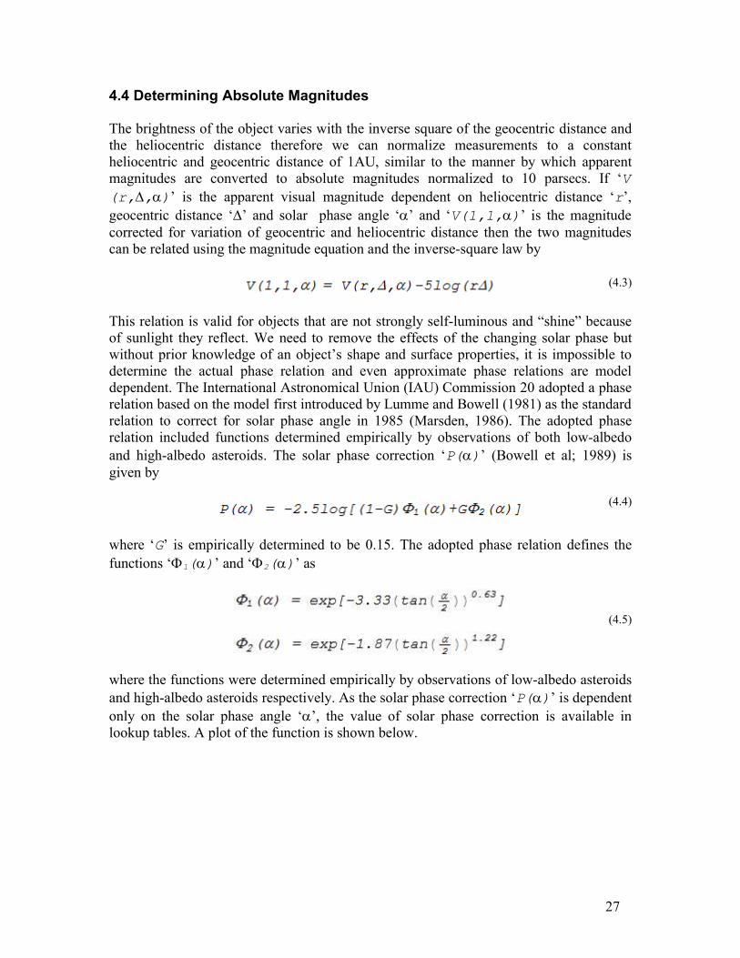
The brightness of the object varies with the inverse square of the geocentric distance andthe heliocentric distance therefore we can normalize measurements to a constantheliocentric and geocentric distance of 1AU, similar to the manner by which apparentmagnitudes are converted to absolute magnitudes normalized to 10 parsecs. If ‘V(r,,)’ is the apparent visual magnitude dependent on heliocentric distance ‘r’,geocentric distance ‘’ and solar phase angle ‘’ and ‘V(1,1,)’ is the magnitudecorrected for variation of geocentric and heliocentric distance then the two magnitudescan be related using the magnitude equation and the inverse-square law by

This relation is valid for objects that are not strongly self-luminous and “shine” becauseof sunlight they reflect. We need to remove the effects of the changing solar phase butwithout prior knowledge of an object’s shape and surface properties, it is impossible todetermine the actual phase relation and even approximate phase relations are modeldependent. The International Astronomical Union (IAU) Commission 20 adopted a phaserelation based on the model first introduced by Lumme and Bowell (1981) as the standardrelation to correct for solar phase angle in 1985 (Marsden, 1986). The adopted phaserelation included functions determined empirically by observations of both low-albedoand high-albedo asteroids. The solar phase correction ‘P()’ (Bowell et al; 1989) isgiven by

where ‘G’ is empirically determined to be 0.15. The adopted phase relation defines thefunctions ‘1()’ and ‘2()’ as

where the functions were determined empirically by observations of low-albedo asteroidsand high-albedo asteroids respectively. As the solar phase correction ‘P()’ is dependentonly on the solar phase angle ‘’, the value of solar phase correction is available inlookup tables. A plot of the function is shown below.

27

(4.3)

(4.4)

(4.5)

We obtain absolute magnitudes from ‘V(1,1,)’ using

where ‘V(1,1,0)’ is the absolute magnitude i.e. the apparent visual magnitude ‘V(r,,)’ normalized to a geocentric and heliocentric distance of 1AU and zero phaseangle. The apparent magnitude can be expressed in terms of the absolute magnitude usingthe above equations as

Several asteroids exhibit a non-linear decrease in the apparent magnitude as the solarphase angle approaches zero (i.e. as the object approaches opposition). The objecttherefore appears significantly brighter near opposition. This marked change in theapparent magnitude, when the object is near 0is known as the opposition effect. Thesolar phase correction based on the model of Lumme and Bowell using the empiricallydetermined adopted by the IAU is appropriate for many asteroids and includes theopposition effect. The solar phase correction is zero for zero phase angle and increasesnon-linearly with increase in phase angle while the phase angle is small (see Fig. 4.7).However, there are asteroids that do not exhibit an opposition effect (French, L.M. 1987).

28

(4.6)

(4.7)

Figure 4.7: A plot of the solar phase correction, ‘P()’. The solar phase relation is non-linear below 5degrees and becomes significantly non-linear again above 100 degrees. The phase relation wasempirically determined by studying 74 asteroid phase curves, Mercury, the Moon and other objects(Bowell et al; 1989).

5. ANALYSIS AND RESULTS

5.1 Period Determination Using Phase Dispersion Minimization

As the outer-belt object rotates about an internal axis, the amount of light it reflects, andtherefore its absolute magnitude, is a periodic function of time. We do not havecontinuous measurements of magnitude with time, but rather measurements of themagnitude at different times. We use the phase dispersion minimization (PDM) algorithmdeveloped by Stellingwerf (1978), to determine possible rotation periods of 279 Thule.

If the data consists of ‘N’ observations (i.e. i = 1, 2, 3,…, N) of the magnitude ‘x’ withmean

where the ith observation is represented by the magnitude ‘xi’ determined at some time‘ti’. The variance ‘2’ of the magnitude ‘x’ is

The algorithm divides the data into ‘M’ (i.e. j = 1, 2, 3,…, M) distinct bins with the jth

bin containing ‘nj’ data points picked such that they have similar values for the rotationalphase ‘i’, determined assuming some rotational period ‘’ such that

If the jth bin containing ‘nj’ data points has a bin variance denoted by ‘sj2’, computed in

exactly the same manner as the variance for the ‘N’ data points, then the overall varianceof all the samples, ‘s2’ is

The algorithm defines the statistic ‘’ as the ratio of the overall variance to the varianceof the magnitude ‘x’

The algorithm repeats the procedure for several trial periods ‘’, and determines theminimum value of ‘’. The statistic is minimized when the overall variance of the bins‘s2’ is minimized. This corresponds to when the trial period ‘’ is close to the true periodas when this condition is met, data from each bin are from the same region of the true

29

(5.1)

(5.2)

(5.3)

(5.4)

(5.5)

lightcurve, and therefore have the same rotational phase. Consequently, the variance ofeach bin ‘sj

2’ is minimized. PDM is the standard method to determine the rotation periods of object whose lightcurvehas been discretely sampled at different rotational phases. IRAF therefore includes animplementation of the PDM algorithm, using the pdm routine defined under noao>astutilpackage. The routine accepts a list of absolute magnitudes, associated errors and theobservation times that correspond to the absolute magnitudes. The routine then searchesfor the period that minimizes ‘’ within a range of periods defined by the user, andoutputs the results graphically.

5.2 The Magnitude Equation and Size Ratios

Using the observed difference in the absolute magnitude of the lightcurve, we can place alower limit on the ratio of the comet’s dimensions using the magnitude equation

where ‘MA-MB’ is the difference between the observed minimum and maximum absolutemagnitude, and ‘IA’ and ‘IB’ are the intensities that correspond to the observed minimumand maximum magnitude. The observed intensity is proportional to the area that theobject presents towards the earth and therefore

where ‘SA’ and ‘SB’ are the surface areas presented towards the earth. Furthermore, if weassume that the surface area presented towards the earth is the projection of a sphericalobject onto a plane, then the surface areas SA and SB are given by the standard formula forthe area of a circle, with diameters ‘lA’ and ‘lB’ respectively.

While we cannot extract the actual dimensions of the object using this technique, we cancombine it with radio observations of the object by the Infrared Astronomical Satellite(IRAS) to give some sense of scale for the object.

30

(5.6)

(5.7)

(5.8)

5.3 Results

The results of photometric analysis are given in Table 5.1. Instrumental magnitudes weredetermined after the data was bias corrected and flat-fielded, using aperture photometrywith a 12.5 pixel radius circular aperture. We transformed instrumental magnitudes intothe Johnson-Kron-Cousin system using photometric calibrations of faint stars observedby Landolt (1992), are given in Table 5.1.

TABLE 5.1: RESULTS

Object V(r,,) V(1,1,0) V-R Size ratio279 Thule 14.66 0.01 8.66 0.44 0.03 1.26:1C/2002 CE10 17.57* 0.01 13.11* 0.54* 0.02 -

5.4 Results for 279 Thule

We observed 279 Thule on six nights (2003 Oct 14 and Oct 16 – 20) at solar phase anglesbetween 1.5 and 2.5 degrees with the telescope tracked at the sidereal rate. All data fromthe first night of observing (2003 Oct 14) is rejected as conditions were not photometric.

The object’s apparent sky motion is small and we do not believe that tracking at thesidereal rate introduced any significant errors. We find the object has a mean absolutemagnitude of 8.660.02. This absolute magnitude was computed using the phase relationadopted by IAU as standard. The absolute magnitude was found to decrease over theobserving run as the solar phase angle increased (see Fig. 5.1). This trend might be anartifact of imaging a different section of the lightcurve each night. If our observationssampled a section of the lightcurve that was lower in magnitude, than the section sampledthe previous night then it would account for the trend. This would imply a rotationalperiod that is less than sub-multiples of 24 hours. If this is the case, then no furtheranalysis of the trend can be done.

However, the trend might also be caused by the IAU standard solar phase correctionrelation ‘P()’ defined in Bowell et al. (1989) being an ill-suited phase relation for 279Thule. If the phase correction ‘P()’ increases too rapidly with phase angle, then thecalculated absolute magnitude decreases with increase in phase angle. This artificialbrightening with increase in phase angle would be an entirely unphysical effect, and adifferent phase relation for 279 Thule would be required.

The above scenario is given more credence by observations of objects similar to 279Thule by French (1987), which do not exhibit an opposition effect. The L5 Trojans 1173Anchises and 2674 Pandarus that were found not to exhibit an opposition effect havebeen classified as either C or P, and D type asteroids respectively; 279 Thule has beenclassified as a D type asteroid. All of these families are redder than most outer-beltasteroids. As discussed earlier, the IAU phase relation based on the Lumme and Bowellmodel, contains empirically determined functions that match the behavior of several low-

31

* likely contamination by coma makes these results suspect

albedo and high-albedo asteroids that exhibit an opposition effect. The differencebetween the colors of C, D and P type asteroids and other outer-belt objects suggests thatthese asteroids have different surface properties than other outer-belt objects, especiallythose that are adequately explained by the IAU phase relation. The observations byFrench show that at least some asteroids obey a different phase relation than the onegiven by Bowell et al. (1989).

As we observed 279 Thule near opposition, we can carry this analysis further. If theLumme and Bowell model is accurate for the object, then as we are moving away fromopposition the apparent magnitude as a function of solar phase angle should show a non-linear increase, corresponding to a drop in brightness. A plot of the apparent magnitudedependent on solar phase angle ‘V(1,1,)’ does increase with solar phase angle (seeFig. 5.2). We assume a linear phase relation to convert from apparent magnitudedependent on solar phase angle to absolute magnitudes i.e.

32

Figure 5.1: Absolute magnitudes, with computed errors in the apparent magnitude from each night. Theabsolute magnitudes show a decreasing trend (the vertical axis is inverted) corresponding to increasingbrightness. The vertical scatter within each night is due to the asteroid rotation. A best-fit line is added tohighlight this trend and has no physical meaning. The trend might be an artifact of sampling a differentregion of the lightcurve each night. In particular, if we sampled a section of the lightcurve that was at alower average magnitude than the previous night’s section then it would account for the decreasing trend inmagnitude. The trend might also be accounted for by the IAU standard solar phase correction beingunsuitable for objects that do not exhibit an opposition effect. We cannot conclusively exclude thispossibility, which is indeed the case for some asteroids (French, L.M., 1987).

as a consequence of equation 4.6. A best fit for ‘V(1,1,)’ as a linear function of thesolar phase angle reveals that the decrease in magnitude can be linear. We do not havesufficient coverage of the solar phase angle to rule out a non-linear decrease. If we coulddetermine the shape of the lightcurve from Fourier analysis, we could normalize theapparent magnitudes to remove the rotational component of the lightcurve. This wouldlead to a considerably more definitive linear phase function fit. However, we do not havesufficient coverage of the rotational phase to perform a meaningful Fourier analysis andcannot carry this analysis further at present.

33

(5.9)

(5.10)

Figure 5.2: Apparent magnitudes, normalized to a heliocentric and geocentric distance of 1AU as afunction of the solar phase angle. The vertical scatter is caused by the rotation of the object about its axis.The apparent magnitude increases with increase in solar phase angle (note the vertical axis is inverted). Wecannot conclude that this is an opposition effect as we have do not have sufficient solar phase anglecoverage to observe any non-linear decrease in brightness. Indeed the observed increase in brightness canbe fit with a linear phase relation. We cannot therefore exclude the possibility that the observed trend ofdecrease in absolute magnitude evident in Fig. 5.1 is caused by the unsuitability of the IAU solar phaserelation (Bowell et al; 1989) for 279 Thule, as was found to be the case for two similar objects 1173Anchises and 2674 Pandarus (French, L.M., 1987). The discontinuity in magnitudes at phase angles of 1.7-1.8 and 2.2-2.3 is artifact of ephemeris that report phase angle to a tenth of a degree. The slope of the linearphase relation is more affected by the vertical scatter than this discontinuity and using more accurate valuesof phase angle will not change the fact that the magnitudes can be modeled by a linear phase relation.

All the remaining results in this section assume solar phase correction given by thestandard IAU phase relation. We stress that the IAU phase relation is sufficient forseveral asteroids, but cannot describe the phase relation for all asteroids satisfactorily asshown by French (1987) and there is no compelling evidence that justifies using this solarcorrection for 279 Thule. We believe that caution must be used when applying solarphase angle corrections to C, D and P type asteroids, as they may have different surfaceproperties from other outer-belt asteroids for which the phase relation was derived. Werecommend further observations of these objects including 279 Thule near oppositionover as wide a range of solar phase angle as is possible.

279 Thule was studied by Zappala et al. (1989) from 1984 Aug 21-23 in UBV usingmultiple telescopes at the European Southern Observatory (ESO) at solar phase angleswith values (for each night) of 2.68, 2.93 and 3.18. The study did not correct for solarphase angle and reports mean apparent magnitudes dependent on solar phase angle (foreach night) as 8.853, 8.856 and 8.878. These values match well with our apparentmagnitudes ‘V(1,1,)’ but at a lower range of phase angle. The discrepancy is smallgiven the almost 19 years between the two sets of observations. The Planetary DataSystem (PDS) does give an absolute magnitude of 8.57 for 279 Thule based on this studyand assuming the IAU solar phase relation. Again, this discrepancy is small given thetime between the two sets of observations. Assuming this absolute magnitude, the IRASMinor Planet Survey quotes an effective diameter of 126.593.7 and mean albedo of0.04120.003.

The maximum observed difference in the absolute magnitude of 279 Thule is 0.07 andthe maximum observed difference on any single night is 0.05. We prefer to report the sizeratio using the second number as the phase angle varied much less on any given nightthan across the entire run. This difference in magnitude corresponds to a size ratio of1.26:1. This represents a least size ratio and the actual variation of the lightcurve may behigher. Zappala et al. report an amplitude variation of the lightcurve of 0.060.01.

We attempted to extract a rotational period for 279 Thule using PDM. A high resolutionPDM scan (see Fig. 5.4) determined the minimum value of the statistic ‘’ to occur at aperiod of 7.60.5 hrs (hereafter, minimum period), which is comprable to the previouslyreported period of 7.440.01 hrs (Zappala et al; 1989). The error is computed using thewidth of the pdm scan near the minimum. A better estimate for the period requires morerotational phase coverage. Another period of 11.3 hrs was also found in the data (see Fig.5.3). The pdm routine reports the first period as the true minimum in a high-resolutionscan. The second period is almost exactly 1.5 times the minimum period. The structurearound the minimum period is similar to the structure around the second period, and itappears that the structure around the second period is also scaled by this factor of 1.5. Aperiod at 5.6 hrs is also found but is not as likely as the first two periods. It is almostexactly 0.75 times the minimum period. Interestingly, the structure around the minimumperiod also appears to be repeated around the 5.6 hrs period and scaled by a factor of0.75. This aliasing is the result of insufficient coverage of the rotation phase. There issome uncertainty in the period because of aliasing, but we believe that the similaritybetween previous photometric measurements and period (Zappala et al; 1989)and ours

34

provides a strong case in favor of a period of 7.60.5 hrs determined by pdm to be theperiod that minimizes the scatter in a trial lightcurve.

35

Figure 5.3: A PDM scan for asteroid 279 Thule reveals that the minimum value of the statistic ‘’ (theta)occurs for a period of about 0.315-d or 7.6 hrs. The deep dip to the right of the minimum at approximately0.470-d represents another candidate period of 11.3 hrs. We cannot totally reject this candidate period usingPDM, as the value of ‘’ for both periods is very comparable. The dip at approximately 0.235-d is simply halfthe 0.470-d period. Multiple periods such as these are a consequence of insufficient phase coverage for theobject, and the problem that they present can only be resolved by simultaneous observations from anotherobservatory in the world, or by observations of the same asteroid at a different epoch. A higher resolution scanto compare the two candidate periods is given below.

Figure 5.4: A PDM scanwith a smaller baselineyields higher resolution. Thisscan allows for quantitativecomparison of the two mostlikely periods – the two lowdips in the graph symmetricabout 0.316-d and 0.470-drespectively. This PDM scanalso returned the 0.316-dperiod as the true period.The FWHM of the PDMscan near the minimumperiod is 0.02-d and we usethis number to put a lower-bound on the error in theperiod. A better period canbe determined with morerotational phase coverage.

5.5 Results for C/2002 CE10 (LINEAR)

C/2002 CE10 (LINEAR) was tracked siderealy from night 1 through 3. Its elongatedappearance was thought to be the result of cometary activity that had been observed usingthe 8.2m Subaru telescope in August 2003 (Takato et al; 2003). However, when wetracked the telescope to compensate for the sky motion of the object, it became apparentthat the elongation was entirely the result of the object’s rapid sky motion. We thereforereject all data from nights 1 through 3. In addition, night 1 proved un-photometric. Afailure of the telescope focus system on night 7 led to a halt in observing for more than anhour. CTIO personnel expertly repaired the problem and we resumed observing, but wefound the object to be at an unacceptably high and increasing airmass. The fewobservations of the object made before the failure were not used in photometry as we hadnot made observations of standards at comparable airmass that early in the night.

The object was observed by Jewitt (2005) on 2003 Jan 8 at the 10m Keck telescope, andwas found to have a mean absolute red magnitude of 13.120.02, and a mean V-R colorindex of 0.560.03. This gives an absolute visual magnitude of 13.680.05. This value ishigher than our mean absolute visual magnitude of 13.110.01. This indicates that theobject was fainter in January. However our mean V-R color index of 0.540.02, agreeswith the given value. Jewitt also observed the object on 2003 Aug 28 at University ofHawaii (UH) 2.2-m telescope. He reports a mean absolute red magnitude of 12.530.02for this date and a mean V-R color index of 0.530.02, and therefore a mean absolutevisual magnitude of 13.060.04. This is in much closer to our result, indicating that theobject’s brightness in August is very close to its brightness in October. The Subaruobservations of a faint tail in August 2003 provide the explanation for the 0.62 decreasein magnitude from January to August 2003. The corresponding increase in brightness iseasily explained if the comet showed a coma. However, it is unlikely that a coma wouldcause a uniform increase in all absolute magnitudes, which is needed to explain the lackof variation in the V-R color from January to October, and other indices from January toAugust.

Jewitt argues that if the coma were sufficiently faint, it would not alter the color indices,as these are dependent only on the properties of the nucleus. We feel that this claim isdifficult to justify, as our observations cannot distinguish between coma and nucleus, asJewitt claims is possible with the UH 2.2-m observations. Yet UH 2.2m observations on2003 Aug 28 agree very well with our observations from 2003 Oct 16-18. This impliesthat both sets of observations are almost certainly contaminated by near nucleus coma.This makes all photometry from this period suspect as aperture photometry yields thecombined level of the nucleus and the coma, and an estimation of the background sky-level may not include the level from the coma, which might in addition be highlyvariable. We therefore cannot determine meaningful size ratios. We could not determine arotational period for C/2002 CE10 (LINEAR) using the PDM algorithm, as we were notable to get sufficient phase coverage for this object. Any rotational period would havealso been based on the assumption that the coma remained constant, which is notjustifiable.

36

6. ACKNOWLEDGEMENTS

The author wishes to thank Professor Linda French, for the opportunity to learn from andwork with her, Professors Narendra Jaggi and Gabe Spalding for all their instruction andfor being tolerant of his many questions, and Professor Lew Detweiler for helping himsurvive in the dark worlds of IRAF and electronics. He recognizes that all his Professorsin the department have been mentors and guides, and have taught him considerably morethan physics. He is very grateful to the department for ensuring that none of the physicsclasses he needed were earlier than 10AM.

A very special thanks is due to our telops, Edgardo Cosgrove, who taught the author thebest way by dunking him into the deep end of the pool and demanding he swim, andArturo Gomez who threatened to throw him off the mountain if the seeing didn’timprove and brought him sandwiches. He thanks the technical support provided byPatricio Ugarte and Enrique Schmidt without which we could not have recovered frommalfunctions on our final night. He extends many thanks to all the other CTIO staffwithout which none of this would have been possible.

He is very grateful to all his peers for motivating him, especially Robin Johnson whochecked this document for speling mistake an poor grammar

Finally, he gratefully acknowledges Lisa Ruberstelli and his friends and coworkers at TheCoffee Shoppe, for keeping him well caffeinated during his time at Illinois Wesleyan.

37

REFERENCES

Abell, P. A., Fernández, Y. R., Pravec, P., French, L.M, Farnham, T. L., Gaffey, M. J.,Hardersen, P. S., Kušnirák, P., Šarounová, L., Sheppard, S. S. and Narayan, G. S. 2005,“Characteristics of C/2001 OG108” Icarus, (accepted)

Asher, D. J, Bailey, M. E., Hahn, G. and Steel, D. J. 1994, “Asteroid 5335 Damocles andits Implications for Cometary Dynamics”, MNRAS 267, 26

Bowell, E., Hapke, B., Domingue, D., Lumme, K., Peltoniemi, J. and Harris, A.W., 1989,“Application of Photometric Models to Asteroids”, In Asteroids II, eds. R. P. Binzel, T.Gehrels, and M.S. Matthews

Fernández, Y. R., Lisse, C. M., Ulrich, K. H., Peschke, S. B., Weaver, H. A., A'Hearn, M.F., Lamy, P. P., Livengood, T. A. and Kostiuk, T. “Physical Properties of the Nucleus ofComet 2 P/Encke” Icarus 147, 145

Fitzsimmons, A., Williams, I.P., Lagerkvist, C.-I. and Dahlgreen, M., 1990, “Spectra ofSix Asteroids Obtained at La Palma” MNRAS 247, 26

French, L.M., 1987, “Rotation Properties of Four L5 Trojan Asteroids from CCDPhotometry”, Icarus 72, 325

Hall, D.S. and Genet, R.M., 1982, Photoelectric Photometry of Variable Stars, IAPPP,Minuteman Press

Jewitt, D. 2005, “A First look at the Damocloids”, AJ 129, 204

Lagerkvist, C. –I., Williams, I.P. Fitzsimmons, A. and Dahlgreen, M. 1990, “(279)Thule”, IAU Circular 4992

Landolt, A.U. 1992, “UBVRI Photometric Standard Stars in the Magnitude Range 11.5-16.0 around the celestial equator”, AJ 104, 340

Levinson, H. F. and Duncan, M. J. 1997, Icarus 127, 13

Lumme, K. and Bowell, E. 1981, “Radiative Transfer in the Surfaces of AtmospherelessBodies. I. Theory”, AJ, 88, 1694

Massey, P. 1989, “The Stellar Content of Two OB Associations in the LMC: LH117(NGC 2122) and LH118”, AJ 97, 107

Massey P. 1997, A User’s Guide to CCD Reductions with IRAF

38

Marsden, B. G. 1986, “Notes from the IAU General Assembly Meeting”, MPC No.10193 and 10194

McNaught, R. H., Stevens, B., Helin, E. F., Pravdo, S., Lawrence, K., Hicks, M.,Hovland, E., Bickler, T., Schroeder, J., Scherr, L., Thicksten, R., Deetz, A., McGaha, J.E., Blythe, M., Shelly, F., Bezpalko, M., Huber, R., Manguso, L., Adams, S., Piscitelli, J.,Stuart, J., Sayer, R., Evans, J. B., Viggh, H., Shelus, P. J., Laurie, S. P. and Marsden, B.G. 2002, “2002 CE10”, MPEC No. 2002-C83

Meech, K. J. and Belton, M. J. S, 1989, “(2060) Chiron” IAU Circular 4770

Romanishin, W. 2002, “An Introduction to Astronomical Photometry Using CCDs”,University of Oklahoma

Stellingwerf, R.F. 1978, “Period Determination using Phase Dispersion Minimization”,ApJ 224, 953-960

Takato, N., Sekiguchi, T. and Watanabe, J. 2003, “Comet C/2002 CE10 (LINEAR)”, IAUCircular 8193

Vilas, F. and Smith, B. A. 1985, “Reflectance spectrophotometry (about 0.5-1.0 micron)of outer-belt asteroids - Implications for primitive, organic solar system material”, Icarus64, 503

Walker, A., 2000, “CTIO CFCCD User Manual”

Young, A.T., 1974, Methods in Experimental Physics, Vol. 12, A, Academic Press, NY

Zappala, V., Di Martino, M., Cellino, A., Farinella, P., De Sanctis, G. and Ferreri, W.1989, “Rotational Properties of Outer Belt Asteroids” Icarus 82, 354

39

APPENDIX A

A.1 The Magnitude System

The idea of a magnitude system originated with the Greek astronomer, Hipparchus, whofirst classified stars by how bright they appeared to the naked eye. The brightest stars thatHipparchus could observe were assigned a magnitude of ‘1’, the next brightest ‘2’, and soon; to the faintest stars he could see, he assigned a magnitude of ‘6’. The system, whilesimple, understandably did not take into account the nature of the eye, which is not agood linear detector i.e. an object that emits twice as much light as another, does notappear twice as bright to the eye when we compare both objects with the naked eye. Inaddition, Hipparchus is the source of the inverted scale for magnitudes, as brighterobjects have lower magnitudes.

Astronomers have adjusted the magnitude scale to make it more convenient, and adifference in magnitude of ‘1’ corresponds to a constant brightness ratio. Specifically,Norman R. Pogson at Oxford University suggested that a difference of five magnitudescorrespond to the object of lower magnitude being brighter than the object with a highermagnitude by a factor of 100; a suggestion that was quickly adopted. Finally, the zeropoint of the system was set by arbitrarily defining the magnitude of the star Vega to beexactly ‘0’. Better measurements of the magnitude of Vega, have determined that itactually has a magnitude of 0.03, but the scale had been too long in existence for it to beadjusted for this shift in origin. Thus, we can write the magnitude equation, in a variety ofequivalent forms relating the magnitudes mA, and mB to the intensities IA, and IB.

How bright an object appears to us depends, in part, on our distance from it, specificallybrightness varies as the inverse square of the distance to the object. This makes it difficultto compare the brightness of objects, and so the absolute magnitude ‘M’ is often used. Theabsolute magnitude is defined as the apparent magnitude ‘m’ of an object at a distance of‘dA’ parsecs, when normalized to a distance of 10 parsecs from us. This provides us witha way to compare the brightness of two objects directly, rather than just their apparentmagnitudes. According to the inverse-square law,

This absolute magnitude is just one example of a normalized magnitude system; we cannormalize magnitudes to any distance we choose. Absolute magnitudes for asteroids are

40

(A.1.1)

(A.1.2)

(A.1.3)

(A.1.4)

normalized to geocentric and heliocentric distances of 1AU and 0 solar phase angle.Absolute magnitudes for asteroids are not the same as absolute magnitudes normalized to10 parsecs, despite both being referred to by the same name. Normalization is simply amethod to remove the dependence of magnitudes on distances and provides a method tocompare the brightness of two objects under similar conditions. By convention,instrumental magnitudes are reported with lower-case alphabets and absolute magnitudes,as well as those calibrated to some standard are referred to using upper-case alphabets.

The brightness of an object depends on what wavelength or color of light we are lookingat, as objects have different spectra, and appear brighter in some colors than in others.Therefore, the magnitude of a star also depends on its color. Astronomers therefore splitlight from an object into various ranges of wavelengths using filters. The Johnson-Kron-Cousins BVRI system is just one such system of filters, and is used for most photometry.We can then use the absolute magnitude of a star, which usually refers to its visual or ‘V’magnitude, and its colors ‘B-V’, ‘V-R’ and ‘V-I’ or the difference between themagnitudes in any two filters.

A.2 The Point Spread Function

For photometric purposes, we can approximate all objects that we observe to be pointsources of light as their actual sizes are small compared to their distance from us.However, we can never resolve a true point source, as several factors such as theatmosphere, telescope optics, and the fundamental fact that matter is not continuous,cause a blurring of the image. The largest source of blurring for ground-basedobservatories is the atmosphere. Any function that takes a point source of light, andreturns a blurred image of it, is called a point spread function or PSF.

Mathematically, given some intensity distribution Io(y,z) in the object plane, an areaelement dydz will emit a flux Io(y,z)dydz. The PSF (y,z;Y,Z) causes a fluxdensity of dIi in the image plane, such that

As the input is a point, the intensity distribution in the object plane can be modeled as theproduct of intensity of the point source ‘A’ and two Dirac delta functions, which make theintensity zero everywhere except at the point (yo,zo).

and, because of the integral properties of the delta function, this implies

41

(A.2.1)

(A.2.2)

(A.2.3)

(A.2.4)

Assuming a circular aperture, for a well corrected system, it can be shown that the PSF isnothing but the Airy distribution function, centered on the Gaussian image point (see Fig.A.2.1). A full derivation of this result is available in any textbook on Fourier optics. Inspherical coordinates the intensity in the image distribution in the image plane Ii(r)

where ‘J1’ is the first order Bessel function (of the first kind) (see Fig. A.2.2).

42

Figure A.2.1: When a point source of light undergoes Fourier diffraction through a circular aperture, theresulting intensity distribution in the image plane is called the Airy disk. (Source: Astrophysics, and SpaceResearch Group, University of Birmingham)

(A.2.5)

(A.2.6)

As the Bessel function approaches zero asymptotically, we can never determine the fullintensity distribution of an object. We therefore use fixed aperture photometry, asdescribed in Chapter 4, to estimate the intensity of the object, and therefore get apparentor instrumental magnitudes, using the magnitude equation. A.3 Atmospheric Extinction and the Transformation Equations

As light passes through the atmosphere, photons can either be scattered in randomdirections or absorbed, either partially or completely by molecules. The net result is adimming or partial extinction of the starlight, which can be described in terms of atransparency of the atmosphere. The transparency depends on the wavelength of light,and can be variable across the sky, and with time for example, fine structured and rapidlymoving cirrus clouds make photometry impossible (Hall and Genet, 1982). In order to dophotometry, the transparency must not vary strongly with sky position, and must remainstable throughout the night.

This transparency can be modeled much the same way that opacity is modeled. We canidealize the earth’s atmosphere as a plane parallel layer with uniform opacity along thehorizontal and the vertical. The height of the slab, as measured from the observatory tothe top of the slab is defined as one airmass. The “zenith distance” of a star is the anglebetween the observer’s zenith and the line connecting the observer and the star. The

43

Figure A.2.2: The Airy distribution is expressed using equation. A.2.5. The first order Bessel function, isan oscillatory function that decays with increase in radius from the center. As the distribution is circularlysymmetric, we can make radial profiles of it such as in Fig. 2.5. (Source: Alexei Tokovnin, CTIO)

length of the slab at any given zenith distance ‘z’ is called the airmass ‘X’ and in thismodel (see Fig. A.3.1) can be expressed using the simple relation

There are obvious limitations to the slab model of the atmosphere such as the atmospherenot being a slab. Rather, it curves with the surface of the earth, does not have a welldefined edge, its density and therefore its opacity depends on height, and wavelength oflight. By restricting photometry to small values of the airmass, we can minimize theproblem somewhat. Thus, in this work, we do not use ‘X’ >1.6 to do photometry. Young(1974) give a more accurate formula

that is found to work well up to sec(z) = 4 (Hall and Genet, 1982). If very highaccuracy airmass’ are needed, even down to the horizon, where observations are limitedby light blocks such as other observatories on site, Romanishin (2002) gives

The intensity modeled as decaying exponentially with airmass ‘X’ such that

44

Figure A.3.1: The slab model of the atmosphere can be used to approximate the airmass, using relationA.3.1. The atmospheric extinction is accounted for when solving the transformation equations (equation4.2) to convert from instrumental to magnitudes in the Johnson-Kron-Cousins system.

(A.3.1)

(A.3.2)

(A.3.4)

… (A.3.3)

where ‘Io’ is the intensity that would be observed without the effect of the atmosphere,‘I’ the intensity after atmospheric extinction, and ‘E’ is some constant ofproportionality. Therefore, using the magnitude equation discussed in appendix A.1, theobserved or instrumental magnitude ‘m’ is related to the magnitude that we wouldobserve without atmospheric extinction (i.e. at zero airmass, ZAM) ‘mo’ by

The ZAM color terms (i.e. without atmospheric extinction) are not exactly the same asthe color terms of the standard system. The ZAM color terms depend on the instrumentalmagnitudes which in turn are dependent on the filter system, detector, observing site etc.However, the filter-detector system is chosen to match the standard system as closely aspossible and therefore the differences between the two systems should be small andsystematic. Therefore, the color terms can be modeled as a simple linear transformationfrom the standard color terms, for example,

Combining equations A.3.4 and A.3.5 allows us to account for atmospheric extinctionand detector characteristics, and these transformation equations allow us to convertbetween instrumental magnitudes and magnitudes in the Johnson-Kron-Cousins system.The coefficients of the transformation equations are determined by fitting the measuredinstrumental magnitudes of the standard stars to the magnitudes of the stars as measuredby Landolt (1992).

45

(A.3.4)

(A.3.5)

APPENDIX B

B.1 Charge Coupled Devices

Invented in 1970 by Willard Boyle and George Smith at Bell Laboratories, the charge-coupled device (CCD) has become the standard photo-electronic imaging device inastronomy. CCDs are constructed out of a chip of crystal silicon that is logically dividedinto a two dimensional array of picture elements or “pixels.” The CCD consists ofpolysilicon electrodes or “gates” with metal contacts, separated from a p-typesemiconductor by a thin layer of oxide, usually silicon dioxide. This structure is commonin electronics and is called a metal oxide on semiconductor (MOS) capacitor. Three ofthese MOS capacitors constitute one pixel.

The use of a p-type semiconductor causes the hole concentration at equilibrium to bemuch larger than the electron concentration. When a positive voltage is applied to thegates, it repels the holes and creates a depletion region near the semiconductor-oxideinterface. When the semiconductor is exposed to light, electrons are ejected via thephotoelectric effect, and are attracted towards the gates and accumulate in the depletionregion. Effectively, the electrons are trapped in a potential well. The photocurrent isdirectly proportional to the intensity of the incident light, over a large range of intensities,and therefore the CCD is a linear photosensitive detector. Electronics can control exactlyhow long the gate voltage is applied, and therefore control how long the MOS capacitorsstore charge, or how long the CCD integrates. Thus, CCDs can be shuttered electronicallyas well as physically.

When two gates are sufficiently close to each other, their potential wells merge. If thevoltage of one gate is higher, than the neighboring gate, then electrons will be transferredto the potential well of the gate with a higher potential. A clocking mechanism regulatesthe potential difference between the three gates, and facilitates the transfer of charge fromone gate to another. The third gate separates each pair of gates while the charge istransferred between them. In order to control a gate chain of any length, only threeseparate clocking signals are needed. The clocking signals are square waves with a 120o

phase shift between them. Readout of the CCD involves clocking each row of pixelssimultaneously, and shifting the stored charge, one by one towards a serial register that isconnected to an output amplifier and a digitizer. The output is therefore a pixel-by-pixelrepresentation of the image produced in the CCD. The charge transfer efficiency (CTE) isthe percentage of charge transferred from one pixel to another. Most research grade CCDshave better than 99.999% CTE.

The quantum efficiency (QE) of a CCD is a measure of the efficiency with which incidentphotons are detected. Some incident photons may be reflected, or absorbed in a region ofthe semiconductor from which electrons cannot be absorbed. The QE depends on thewavelength of the incident light. In front-illuminated CCDs, incident photons passthrough the gate structure before they can generate electrons. Silicon has a highabsorption coefficient for short wavelength photons, and therefore front-illuminatedCCDs have low QE in the blue and UV. In back-illuminated CCDs, the incident light

46

falls directly on the silicon crystal that is thinned to around 15-20 microns. This processenhances the QE in the blue and UV. The QE of back-illuminated CCDs is often furtherenhanced by using anti-reflective coatings.

B.2 Quantum Efficiency of our CCD, and Filter Transmission Curves

The percentage of the incident light detected does not depend solely on the QE of theCCD, as the light passes through filters before it is incident on the CCD. The fraction ofthe incident signal that is detected is the convolution of the filters transmission curve, andthe QE curve of the CCD.

47

Figure B.1: The QE curve of the TeK 2K CCD, such as that mounted on the 0.9m SMARTS telescope atCTIO. The CCD has better than 50% QE from 400-850nm. (Source: Alistair Walker, CTIO)

48

Figure B.2: Transmission curves for the set of filters used in this observing run (clockwise from top left)approximate the Johnson ‘B’ and ‘V’, Cousins ‘R’ and Kron ‘I’ filters. CTIO personnel periodically checkthe filters to ensure that their transmission characteristics have not changed significantly. Thetransformation equations allow us to remove the effects of our particular filter system. The Kron ‘I’ filter iswrongly listed as 4x4” as a check of the serial number on the top left of the graph reveals. (Source: RicardoGonzález, CTIO)