HAL Id: hal-01770079https://hal-enpc.archives-ouvertes.fr/hal-01770079

Submitted on 7 May 2018

HAL is a multi-disciplinary open accessarchive for the deposit and dissemination of sci-entific research documents, whether they are pub-lished or not. The documents may come fromteaching and research institutions in France orabroad, or from public or private research centers.

L’archive ouverte pluridisciplinaire HAL, estdestinée au dépôt et à la diffusion de documentsscientifiques de niveau recherche, publiés ou non,émanant des établissements d’enseignement et derecherche français ou étrangers, des laboratoirespublics ou privés.

Performance Assessment of a 3D Hydrodynamic ModelUsing High Temporal Resolution Measurements in a

Shallow Urban LakeFrédéric Soulignac, Brigitte Vinçon-Leite, Bruno J. Lemaire, José ScaratiMartins, Céline Bonhomme, Philippe Dubois, Yacine Mezemate, Ioulia

Tchiguirinskaia, Daniel Schertzer, Bruno Tassin

To cite this version:Frédéric Soulignac, Brigitte Vinçon-Leite, Bruno J. Lemaire, José Scarati Martins, Céline Bonhomme,et al.. Performance Assessment of a 3D Hydrodynamic Model Using High Temporal Resolution Mea-surements in a Shallow Urban Lake. Environmental Modeling & Assessment, Springer, 2017, 22 (4),pp.309-322. �10.1007/s10666-017-9548-4�. �hal-01770079�

Performance Assessment of a 3D Hydrodynamic Model Using High

Temporal Resolution Measurements in a Shallow Urban Lake

Frédéric Soulignac, Brigitte Vinçon-Leite, Bruno J. Lemaire, José R. Scarati Martins, Céline Bonhomme,

Philippe Dubois, Yacine Mezemate, Ioulia Tchiguirinskaia, Daniel Schertzer, Bruno Tassin

1 Introduction

Urban lakes provide many ecosystem services: regulation services (flood control, biodiversity conservation,

coolness island), cultural services (recreational activities, angling, tourism, education), and ecological services

(nature protection areas). At a global scale, the vast majority of lakes has an area smaller than 1 km2. Taking into

account the very small lakes (≤0.001 km2), the total area of lakes was estimated between 3.1 106 km2 [1] and 4.2

106 km2[2]. In urban areas, the lakes are predominantly small and shallow. For instance, in the Île-de-France region

around Paris, the number of lakes and ponds of surface larger than 0.01 km2 is estimated around 990 [3], but 99%

of them are very small, with an area lower than 0.5 km2, the minimum area of the lakes monitored in the frame of

the European Water Framework Directive.

Whereas large, deep lakes of long water time residence integrate the dynamics of weather and their tributaries over

seasonal time scale, shallow lakes can strongly react within a few hours. The meteorological forcing affects the

greater part of the water column. Their smaller stability can more easily be overruled by air cooling or by the

momentum brought by wind or inflows, causing the alternation of periods of thermal stratification and mixing.

These lakes are called polymictic as opposed to the monomictic or dimictic deep lakes. In particular, summer

mixing episodes cause the transfer of heat flux to the lake bottom and high vertical velocities close to the bottom

favoring sediment resuspension leading to nutrient release and increased turbidity [4]. The spatial distribution of

the external forces can be very heterogeneous: local stormwater input, differential shadowing by the surrounding

buildings, heterogeneous bottom roughness due to submersed macrophytes and artificial bottom. Therefore, the

hydrodynamic processes in shallow lakes are complex.

Hydrodynamics strongly affect the distribution of water quality components and ecological processes. In many

cases, the goal of 3D modeling is to understand and predict the water quality evolution of a lake in response to

changing external pressures: climate forcing, nutrient loading, and pollutant input [5, 6, 7]. The hydrodynamic

sub-model is a tool aimed at providing the spatial water temperature distribution, the water current field, and the

spatial patterns of mixing to the coupled water quality model. Three-dimensional numerical modeling is a

compulsory tool in order to understand the hydrodynamic behavior of shallow lakes and its influence on the fate

of pollutants and ecosystem functioning, but also to interpret the results of discrete chemical and biological

campaigns since lake conditions may vary considerably between the campaigns. But hydrodynamics of small and

shallow lakes are less studied than in large lakes and 3D modeling attempts are rare.

In small shallow lakes at intermediate latitudes, current velocities are generally very low (mm s−1 to cm s−1). The

acquisition of such low velocities demands high sensitivity current meters [8]. The scarcity of this type of data

frequently limits the validation of three-dimensional (3D) hydrodynamic models and therefore their practical

applicability [9]. More generally, in order to understand the hydrodynamic behavior of these lakes, high resolution

and high frequency measurements are necessary. Indeed, a survey of scientific references performed on Web of

Science in April 2016 with the key words “hydrodynamic model” (topic) and “large lake*” (title) against

“hydrodynamic model” and “small lake*” showed that there are about 5 times more papers on the modeling of

large lakes than small lakes, respectively 34 versus 6.

In this study, we present the first validation of a 3D hydrodynamic model on a small shallow lake, Lake Créteil,

France, with high resolution and high frequency measurements. Our objective was to assess the model

performance: can it reproduce the alternation of thermal stratification and mixing, internal waves and spatial

heterogeneities of current speed and water temperature? We present the calibration of the model on a 1-month

period with continuous water temperature measurements and current speed profiles. We then present the model

performance assessment on the same variables as well as on the net heat flux at the surface and water temperature

at two other measuring points for 18 periods of around a month, from May 2012 to January 2014. The model

capability to describe correctly the alternation of mixing and stratification periods is also discussed.

2 Material and Methods

2.1 Study Site

Lake Créteil is located in an urbanized area in the south-east of Paris, France (Fig. 1). Its area is 0.4 km2, its

perimeter 4 km, its length 1.5 km, its width varies between 250 and 400 m. Its mean depth is 4.5 m, with a

maximum of 6.5 m, and its volume is 1.9 106 m3. The northern part is shallower than the southern part. The lake

was created as an extraction quarry of gravel and gypsum between 1940 and 1976 and was dug in the former

alluvium of the Seine river, near its confluence with the Marne river [10]. The quarry was transformed into an

urban lake in the middle of the 1970s; it includes a recreation center of Île-de-France regional council with a park

of 0.62 km2 on the lake’s western bank. The lake is surrounded by buildings in the North, East, and South-East.

The lake is fed by groundwater which flows mainly from the Marne river to the Seine river due to a 1 m difference

in the normal level of the navigation reaches, by storm water from a 1 km2 urbanized area in the East and by direct

precipitation. The water level is regulated by a fixed gate on the western bank. The lake is used for recreational

activities (boating, sailing, angling, etc.), to water the park on the western bank, to clean the roads, and for

roadwork.

Fig. 1 Location of Lake Créteil and of the measuring points P close to the storm water inlet, C in a more central location,

and R close to the lake outlet

2.2 Measuring Equipment and Database

A transmitting monitoring buoy equipped with a meteorological station and a sensor chain as well as two other

sensor chains were installed in Lake Créteil in May 2012. They measured continuously vertical profiles and

horizontal transects of water temperature in the lake over 21 months.

The monitoring buoy (Precision Measurement Engineering Environmental Sensor Platform, LakeESP) was

moored in the deepest region of the lake at point C (Fig. 1) and has worked continuously since May 11, 2012. The

meteorological station, located 2 m above the lake surface, measures wind speed and direction, liquid precipitation,

barometric pressure, air temperature, relative humidity (Vaisala Weather Transmitter WXT520), and net total

radiation (Kipp and Zonen NR Lite2). The underwater chain is equipped with five temperature sensors (accuracy

0.01∘C). The sampling time-step is 30 s. The sensors are located at fixed heights above the lake bottom which

correspond to average depths of 0.5, 1.5, 2.5, 3.5, and 4.5 m.

Two other sensor chains were also installed on buoys on October 25, 2012. One is located at point P in front of

the municipal storm-water inlet and the other at point R in the southern part of the lake near a reed bed and the

lake outlet (Fig. 1). The three points P, C, and R are aligned with 250 m between P and C and 150 m between C

and R. These additional chains are composed of two temperature sensors (nke Instrumentation SP2T) at 0.5 and

2.5 m depths and one multiparameter probe (nke Instrumentation MP5) which measures water temperature

(accuracy 0.01∘C), dissolved oxygen and chlorophyll fluorescence at 1.5 m depth. Variables are sampled every 30

s as on the central measuring station.

A high-resolution current profiler (2 MHz Nortek Aquadopp) was mounted head upwards on an rigid aluminum

frame near the central measuring station at point C from September 17, 2013 to October 15, 2013. The velocity

profiles were sampled every 3 m and spread from 4.5 to 1.5 m depth with a vertical resolution of 2.3 cm.

Bathymetry was measured in September 2014 with an echo-sounder (HumminBird 798ci HD SI Combo).

Between 14 May 2012 and 17 January 2014, the water transparency was measured monthly at points P, C, and R

with a Secchi disk.

2.3 Model Configuration

The 3D hydrodynamical model Delft3D-FLOW was used. It solves the Navier-Stokes equations for an

incompressible fluid, under the shallow water and the Boussinesq assumptions. The system of equation consists

of the continuity equation (Eq. 1), the two horizontal equations of motion (Eqs. 2 and 3), the equation of motion

in the vertical direction being reduced to the hydrostatic pressure equation, and the transport equation of heat

(Eq. 4). This set of partial differential equations in combination with an appropriate set of initial and boundary

conditions is solved on a finite difference grid with current velocities defined on cell faces and scalar variables at

cell centres. Delft3D-FLOW was fully described in the user manual [11]. Here, we present the model configuration

we used.

x, y, and z are Cartesian coordinates (m). t is time (s). u, v, and w are the three components of the water velocity

(m s−1). T is the water temperature (K), ρ 0 is the water density (kg m−3) and p is the pressure (Pa). ν H and ν V are

the horizontal and vertical eddy viscosities (m2 s−1). D H and D V are the horizontal and vertical coefficients of eddy

diffusivity of heat (m2 s−1). S is the source of heat per unit volume (W m−3) and c p w is the water specific heat (J

K−1kg−1). Molecular viscosity and diffusivity are neglected.

The horizontal surface of the lake was meshed with 981 Cartesian cells of 20 m x 20 m. In order to obtain a good

simulation of the water column stratification, the Z-model was used with 18 layers of 33 cm. The sensor depths

correspond to cell centers. Too thin bottom layers were remapped automatically in order to better represent the

current speed close to the bottom.

The eddy viscosity and diffusivity of heat are anisotropic. In the vertical direction, the eddy viscosity ν V and the

eddy diffusivity of heat D V were calculated using the k- turbulence closure model. Two parameters are used in

Delft3D-FLOW to reproduce subgrid horizontal motions and fluxes, the background (minimum) values of the

horizontal eddy viscosity νbackHνHback and diffusivity of heat DbackHDHback. We used as fixed values for

these parameters the time and space averages of the eddy viscosity and diffusivity of heat computed by 2D

horizontal large eddy simulation on the calibration period (Table 1). The time and space averages of the eddy

viscosity and diffusivity of heat computed by 2D horizontal large eddy simulation on the calibration period were

then used as fixed parameters for the 3D simulations.

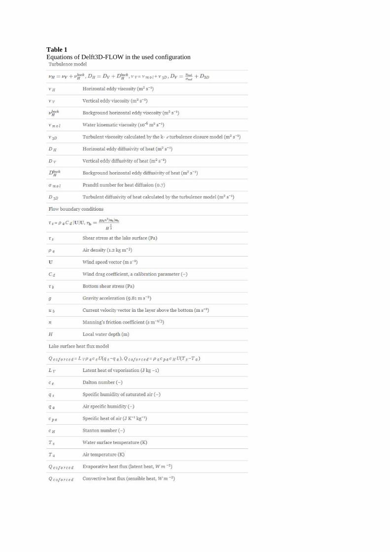
Table 1 Equations of Delft3D-FLOW in the used configuration

This configuration enabled to prescribe different levels of turbulence in vertical and horizontal directions. A

sensitivity analysis on the mean absolute error (MAE) of water temperature showed that no additional mixing was

necessary: we left the Ozmidov length L z parameter which triggers mixing at the thermocline, the background

vertical eddy viscosity, and the background vertical eddy diffusivity of heat to their default value, zero.

The shear stress at the surface of the lake due to the wind was modeled with a constant wind drag coefficient, a

calibration parameter (Table 1). The shear stress at the bottom of the lake was modeled with the Manning

formulation. A value of 0.02 s m−13−13 was adopted for the Manning coefficient because the bottom of the lake,

a former gravel quarry, is smooth. The vertical wall roughness of the banks was neglected.

Heat fluxes through the banks and the lake bottom were neglected. The heat surface model that we chose to use

was adapted from Gill [12]. The latent heat flux by forced convection is parameterized by the Dalton number c e ,

the sensible heat flux by forced convection, by the Stanton number c H , and the latent and sensible heat fluxes by

free convection, by the coefficient of free convection C F r C o n (Table 1). These coefficients were calibrated for

the North Sea [13] and applied successfully for Lake Créteil.

In the water column, light dampens according to Beer-Lambert law. The extinction coefficient was considered as

a calibration parameter. We verified that its value is close to the extinction coefficient calculated from the water

transparency measurements (Secchi depth).

The water density was calculated according to UNESCO formulation [14] with a salinity of 0.75 ppt corresponding

to the observed specific conductance of 1500 μS cm−1. This relatively high salinity is due to the geological calco-

carbonated nature of the catchment.

Water level variations were neglected; they never exceeded 3% of the water height over a simulation period.

Simulations were initialized with water temperature observed at the measuring station on the first day of the

simulation. The water was supposed to be at rest, an usual assumption in 3D hydrodynamic simulation. Simulations

were started and stopped at midday. Thirty-second wind direction and speed, air temperature, relative humidity,

and precipitation recorded at point C and hourly incident solar radiation and cloud cover measured at the nearest

weather station located at Orly Airport, 10 km west of the lake were used to force the simulations.

An explicit time integration method was used. The computational time step was set equal to that of the

meteorological variables, 30 s. This value respects the Courant-Friedrichs-Levy stability criterion. The equation

of momentum is solved by a multidirectional upwind explicit numerical scheme and the equation of heat by the

second Van Leer numerical scheme.

The total net radiation through the lake surface, sum of the incident solar radiation reduced from albedo, the net

atmospheric radiation, and the back radiation of the lake surface was computed separately with Delft3D-FLOW

equations in order to compare the simulated values to the measurements.

2.4 Model Calibration and Performance Assessment

A period of 28 days between between 17 September 2013 and 15 October 2013 was chosen for calibration because

this period presented a full stratification and also all measurements were available, including current profiles. Only

two parameters, the wind drag coefficient and the light extinction coefficient, were calibrated. The trial and error

method was used to calibrate these parameters in order that simulated profiles of hourly water temperature and

current velocity at point C best fitted observations. The MAE was used as performance indicator. Simulated and

observed hourly total net radiation at the lake surface and water temperature at points C, P, and R were compared

graphically. MAE was computed for the total net radiation, at the five depths of the sensors for water temperatures

at point C and at the three depths of the sensors for water temperatures at points P and R. The hourly resolution

used for this comparison is consistent with the time scale of biological processes which coupled hydrodynamic-

biogeochemical simulations could later reproduce. Moreover, time averaging is required to compare the evolution

of temperatures simulated in a large cell (several m3) to much more fluctuating temperatures measured at a point.

Only graphical assessment was performed for current velocities.

The model was then run with the same set of parameters, namely the wind drag coefficient and the Secchi depth

during 18 other time periods between two consecutive monthly field campaigns. They covered a wide range of

hydrodynamic situations in the lake and of meteorological forcing. For each simulation period, the measured

temperature profiles were used as initial conditions. Comparison between observed and simulated values was

performed as described for calibration. For synthesizing multiple aspects of the model performance, we used a

single diagram, the Taylor diagram [15]. This diagram provides a summary of two statistical indicators of model

performance: the linear correlation coefficient between model results and observed values and the ratio of standard

deviations of simulated and measured values. A global skill index was also computed.

3 Results

This section presents first the results of model calibration based on the discrepancies between model results and

measurements of water temperature and speed at point C, of stratification duration and dates and of the

characteristics of the internal waves (amplitude and frequency). The model verification is then presented based on

the same criteria for 18 simulation periods of around 1 month, from May 2012 to January 2014.

3.1 Model Calibration

The calibration period was chosen between 17 September and 15 October 2013 (28 days). The number of layers

was set to 18 corresponding to a layer thickness of 33 cm. With a higher thickness, the velocities under the

thermocline became much lower than measured. Only the drag coefficient and the Secchi depth were calibrated

(Table 2). Values of wind drag coefficient ranging between 0 and 10−2 were tested. Finally, the wind drag

coefficient was set to 0.0015. For this value, average MAE of water temperature was lowest and the model

reproduced best the current speeds and the amplitudes of internal waves. A Secchi depth of 1 m close to the one

observed during the calibration period, corresponding to an extinction coefficient of 1.7 m−1, was adopted to

reproduce properly the temperature differences between surface (0.5 m depth) and bottom (4.5 m) sensors.

Table 2 Comparison of mesh characteristics and parameter values used for simulations with Delft3D-FLOW on different

lakes (nc: not communicated, na: not applicable)

Hourly means of simulated and observed water temperature and horizontal current velocity at point C between 17

September and 15 October 2013 are plotted on Fig. 2a, b. On Fig. 2c are plotted temperature differences between

points P and R. The temperature evolution is well reproduced (MAE of hourly temperature during the simulation

and over the five depths is 0.48∘C), as well as the alternation between stratification and mixing periods. The water

column was mixed the first day of the simulation and the onset of the stratification was observed on 20 September

2013, whereas the simulation reproduced it one day after, on 21 September. Observed and simulated duration of

stratification was respectively 16 and 15 days. The end of stratification was reproduced by the model at the correct

date on 5 October 2013. The simulated current speeds are very close to the observed ones (Fig. 2b) as well as the

temperature differences between points P and R (Fig. 2c). The capacity of the model to reproduce the low velocity

values in the layers below the thermocline during stratification must be highlighted. Internal waves are observed

in Lake Créteil during stratification periods. An intense internal wave activity was observed during the calibration

period, between 28 to 30 September 2013 when a strong wind episode occurred. The observed internal wave

patterns showed a period of 17 h and a maximum temperature variation of 1.5∘C from peak to peak at 2.5 m depth.

These high fluctuations of water temperature at 2.5 m depth are well reproduced and the period of 17 h was also

captured by the model.

Fig. 2 Calibration period: Hourly mean profiles of observed and simulated water temperature at point C (a), horizontal

current velocity at point C (b), and difference of water temperature between points P and R (c), between 17/09 and

15/10/2013 (observed water temperature at point C and temperature differences are linearly interpolated between

the five measurement depths (0.5, 1.5, 2.5, 3.5, and 4.5 m), the vertical resolution of the velocity profile is 2.3 cm,

the simulated values are linearly interpolated at the centre depth of the 18 computational layers)

3.2 Model Verification

Nineteen simulations were run over the period from 14 May 2012 to 17 January 2014 including the calibration

period. The length of these simulations was about 1 month. Measurements and simulation results of total net

radiation through the lake surface at point C and water temperature at points P, C, and R were compared.

Hourly values of total net radiation varied between −200 and 900 W m−2, and the daily accumulation of total net

radiation varied between −100 and 250 W m−2. Observations were well reproduced during the calibration period

between 17 September 2013 and 15 October 2013. For the 19 simulation periods, MAE between observed and

simulated total net radiations were calculated. They range between 9.9 and 25.7 W m−2. Relative MAE are smaller

from spring to autumn than in winter. It means that the combination of data used as forcing meteorological

variables and the formulation of the radiation part of the heat flux in the model work well.

The capability of the model to reproduce the water temperature and the alternation between stratification and

mixing was assessed. Several stratifications were observed during the study period and their length ranged from a

few hours up to 40 days. The longest stratification period occurred between 30 June and 8 August 2013. The

alternation between stratification and mixing was very well reproduced by the model. The maximal water

temperature of 27.6∘C was observed in July 2013 and the minimum of 2.7∘C was observed in January 2013. Short

inverse stratifications were indeed observed. Observed and simulated water temperature at point C are plotted for

the 19 simulations (Figs. 3 and 4). Temperature MAE at point C are presented in Table 3 and temperature MAE

at points P and R are presented in Table 4. Plots and MAE showed that the model reproduced well the water

temperature at the three points. Water temperature was better reproduced between May and October (spring,

summer, and early autum) 2012 and 2013 than between October 2012 and March 2013 (late autumn and winter):

Temperature MAE at point C over the five depths between March and October 2013 is 0.44∘C and between October

2012 and March 2013 it is 1.41∘C. An overview of the model performance is provided by Taylor diagrams (Fig. 5).

These diagrams present the model performance at five depths, 0.5, 1.5, 2.5, 3.5, and 4.5 m, for 19 simulation

periods. Two metrics are considered for assessing the agreement between model and observations: the linear

correlation coefficient r and the standard deviation ratio σ*. For all considered periods except period 8, from spring

to autumn, at all depths, the results are excellent and very similar with high correlation coefficients and good

standard deviation ratio. The global skill index indicated by the isoline area is close to 1, its maximum value. In

winter, the model performance is lower. During period 8, from 10 December 2012 to 15 January 2013, low

performance indicators are obtained at all depths.

Fig. 3 Observed and simulated water temperature at point C for simulation 1 to 10

Fig. 4 Observed and simulated water temperature at point C for simulation 11 to 19

Fig. 5 Taylor diagrams of the model performance at point C, at 5 depths, 0.5, 1.5, 2.5, 3.5, and 4.5 m depth, for 19

simulation periods (the angle C corresponds to the linear correlation coefficient between model results and

measurements, the x-axis and the y-axis to the ratio of standard deviations of simulated and measured values, σ*)

Table 3

Mean absolute error (MAE) of water temperature in∘C at point C and 5 depths (0.5, 1.5, 2.5, 3.5, and 4.5 m) for

the 19 simulations. Period 16 is the calibration period

Sim. Start Stop 0.5 m 1.5 m 2.5 m 3.5 m 4.5 m

1 14/05/2012 12/06/2012 0.44 0.44 0.49 0.69 0.81

2 12/06/2012 05/07/2012 0.48 0.42 0.40 0.28 0.33

3 05/07/2012 29/07/2012 0.44 0.43 0.44 0.44 0.28

4 29/07/2012 11/09/2012 0.53 0.48 0.51 0.52 0.54

5 11/09/2012 16/10/2012 0.66 0.64 0.64 0.64 0.67

6 16/10/2012 14/11/2012 0.84 0.82 0.79 0.76 0.77

7 14/11/2012 10/12/2012 1.18 1.17 1.17 1.16 1.16

8 10/12/2012 15/01/2013 2.30 2.29 2.29 2.28 2.27

9 12/02/2013 26/03/2013 1.44 1.42 1.39 1.36 1.34

10 26/03/2013 16/04/2013 0.41 0.40 0.38 0.32 0.25

11 16/04/2013 15/05/2013 0.37 0.32 0.32 0.44 0.57

12 15/05/2013 11/06/2013 0.37 0.41 0.39 0.43 0.53

13 11/06/2013 09/07/2013 0.45 0.44 0.45 0.35 0.29

14 09/07/2013 29/07/2013 0.34 0.37 0.32 0.87 0.47

15 29/07/2013 17/09/2013 0.59 0.53 0.52 0.50 0.53

16 17/09/2013 15/10/2013 0.48 0.45 0.47 0.48 0.55

17 15/10/2013 12/11/2013 0.67 0.66 0.64 0.60 0.57

18 12/11/2013 10/12/2013 1.18 1.18 1.18 1.17 1.17

19 10/12/2013 17/01/2014 1.61 1.60 1.60 1.59 1.57

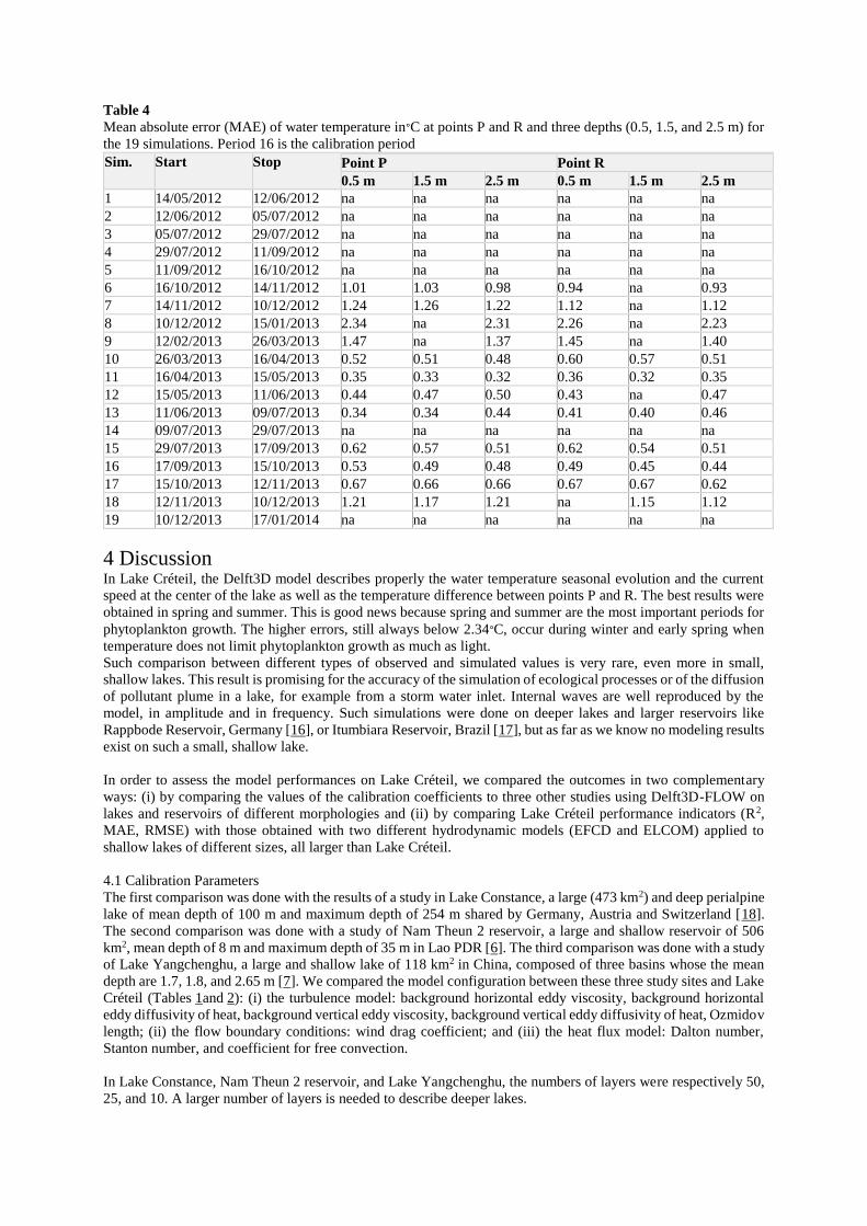
Table 4

Mean absolute error (MAE) of water temperature in∘C at points P and R and three depths (0.5, 1.5, and 2.5 m) for

the 19 simulations. Period 16 is the calibration period

Sim. Start Stop Point P Point R

0.5 m 1.5 m 2.5 m 0.5 m 1.5 m 2.5 m

1 14/05/2012 12/06/2012 na na na na na na

2 12/06/2012 05/07/2012 na na na na na na

3 05/07/2012 29/07/2012 na na na na na na

4 29/07/2012 11/09/2012 na na na na na na

5 11/09/2012 16/10/2012 na na na na na na

6 16/10/2012 14/11/2012 1.01 1.03 0.98 0.94 na 0.93

7 14/11/2012 10/12/2012 1.24 1.26 1.22 1.12 na 1.12

8 10/12/2012 15/01/2013 2.34 na 2.31 2.26 na 2.23

9 12/02/2013 26/03/2013 1.47 na 1.37 1.45 na 1.40

10 26/03/2013 16/04/2013 0.52 0.51 0.48 0.60 0.57 0.51

11 16/04/2013 15/05/2013 0.35 0.33 0.32 0.36 0.32 0.35

12 15/05/2013 11/06/2013 0.44 0.47 0.50 0.43 na 0.47

13 11/06/2013 09/07/2013 0.34 0.34 0.44 0.41 0.40 0.46

14 09/07/2013 29/07/2013 na na na na na na

15 29/07/2013 17/09/2013 0.62 0.57 0.51 0.62 0.54 0.51

16 17/09/2013 15/10/2013 0.53 0.49 0.48 0.49 0.45 0.44

17 15/10/2013 12/11/2013 0.67 0.66 0.66 0.67 0.67 0.62

18 12/11/2013 10/12/2013 1.21 1.17 1.21 na 1.15 1.12

19 10/12/2013 17/01/2014 na na na na na na

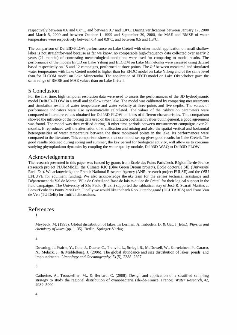
4 Discussion

In Lake Créteil, the Delft3D model describes properly the water temperature seasonal evolution and the current

speed at the center of the lake as well as the temperature difference between points P and R. The best results were

obtained in spring and summer. This is good news because spring and summer are the most important periods for

phytoplankton growth. The higher errors, still always below 2.34∘C, occur during winter and early spring when

temperature does not limit phytoplankton growth as much as light.

Such comparison between different types of observed and simulated values is very rare, even more in small,

shallow lakes. This result is promising for the accuracy of the simulation of ecological processes or of the diffusion

of pollutant plume in a lake, for example from a storm water inlet. Internal waves are well reproduced by the

model, in amplitude and in frequency. Such simulations were done on deeper lakes and larger reservoirs like

Rappbode Reservoir, Germany [16], or Itumbiara Reservoir, Brazil [17], but as far as we know no modeling results

exist on such a small, shallow lake.

In order to assess the model performances on Lake Créteil, we compared the outcomes in two complementary

ways: (i) by comparing the values of the calibration coefficients to three other studies using Delft3D-FLOW on

lakes and reservoirs of different morphologies and (ii) by comparing Lake Créteil performance indicators (R2,

MAE, RMSE) with those obtained with two different hydrodynamic models (EFCD and ELCOM) applied to

shallow lakes of different sizes, all larger than Lake Créteil.

4.1 Calibration Parameters

The first comparison was done with the results of a study in Lake Constance, a large (473 km2) and deep perialpine

lake of mean depth of 100 m and maximum depth of 254 m shared by Germany, Austria and Switzerland [18].

The second comparison was done with a study of Nam Theun 2 reservoir, a large and shallow reservoir of 506

km2, mean depth of 8 m and maximum depth of 35 m in Lao PDR [6]. The third comparison was done with a study

of Lake Yangchenghu, a large and shallow lake of 118 km2 in China, composed of three basins whose the mean

depth are 1.7, 1.8, and 2.65 m [7]. We compared the model configuration between these three study sites and Lake

Créteil (Tables 1and 2): (i) the turbulence model: background horizontal eddy viscosity, background horizontal

eddy diffusivity of heat, background vertical eddy viscosity, background vertical eddy diffusivity of heat, Ozmidov

length; (ii) the flow boundary conditions: wind drag coefficient; and (iii) the heat flux model: Dalton number,

Stanton number, and coefficient for free convection.

In Lake Constance, Nam Theun 2 reservoir, and Lake Yangchenghu, the numbers of layers were respectively 50,

25, and 10. A larger number of layers is needed to describe deeper lakes.

For Lake Yangchenghu, as water temperature was not considered as a state variable, only the background

horizontal eddy viscosity and the wind drag coefficient were compared. In these three water bodies, the background

horizontal eddy viscosity are two or three orders of magnitude larger than in Lake Créteil because larger horizontal

grids were used. In Lake Constance and in Nam Theun 2 reservoir, the background horizontal eddy diffusivity of

heat was set to the same values as the background horizontal eddy viscosity and was also two or three order of

magnitude larger than in Lake Créteil. This is coherent with the previous comparison. Background vertical eddy

viscosity and diffusivity of heat were set to zero in Lake Créteil as well as Lake Constance and Nam Theun 2

reservoir. The Ozmidov length in Nam Theun 2 reservoir is set to zero like in Lake Créteil. These comparison

results show that neither additional vertical mixing nor mixing around the thermocline is required. The latter is

used in strongly stratified lakes with large internal waves.

Regarding the wind drag coefficient, a function of wind speed was used for Lake Constance [18]. This coefficient

increases with the wind speed in order to take into account its influence in the surface roughness. In Lake Créteil,

the fetch length is not such that large surface waves can form and increase the wind drag coefficient. The wind

drag coefficient was set to 0.0005 for Nam Theun 2 reservoir [6] and 0.0025 for Lake Yangchenghu [7]. This

coefficient depends on the type of wind record and on the location of the meteorological station where wind speed

was recorded. Wind speed measured at the meteorological station in Constance as representative data for the wind

characteristics at 10 m height above lake surface was used for Lake Constance [18]. Both wind data computed by

the model of the European Centre for Medium-Range Weather Forecasts (ECMWF) with a 6-h time step and

measurements from two automatic meteorological stations located on the lake with a 10-min time step was used

for Nam Theun 2 reservoir [6]. A constant wind speed of 3 m s−1 from wind data measured in the region around

the lake was used for Lake Yangchenghu [7].

Concerning the parameters involved in the heat flux budget, we used for Lake Créteil respectively 0.0015, 0.00145,

and 0.14 for the Dalton and Stanton numbers and for the coefficient of free convection, close or equal to the default

values. For Lake Constance, an increased Dalton number to 0.0021 was used and the Stanton number was kept to

the default value of 0.00145 [18]. It can be supposed that the coefficient of free convection was set to zero because

the Dalton number was very high. This could have been motivated by the fact that the wind rarely falls to zero on

Lake Constance which means that loss of heat by free convection is negligible compared to forced convection. For

Nam Theun 2 reservoir, slightly increased Dalton and Stanton numbers of 0.0016 were used [6]. Dalton and

Stanton numbers depend also on the height above the surface of the meteorological station where air temperature

and relative humidity are recorded. Nothing was said about the coefficient of free convection.

The comparison of the background horizontal eddy viscosity and diffusivity of heat confirmed that their values

depend on the horizontal grid size and on the current intensity. For Lake Créteil, the wind drag coefficient and the

Stanton and Dalton numbers are set to very close values, 0.0015 and 0.00145. This indicates the reliability of the

meteorological forcing and the accuracy of the surface heat budget and that spatially homogeneity of

meteorological forcings can be assumed for lakes of this size.

4.2 Performance of Three-Dimensional Hydrodynamic Models

In our modeling results, the monthly mean absolute error (MAE) in water temperature ranges between 0.25 and

2.34∘C. The first comparison was done with the study of Lake Yilong using the Environmental Fluid Dynamic

Code (EFCD) model [19]. Lake Yilong has a mean depth of 3.9 m, a maximum depth of 5.7 m, and a surface area

of 28.4 km2. The hydrodynamic model was calibrated with data collected during 15 punctual campaigns over 1

year, from summer 2008 to summer 2009, at three monitoring points. During the calibration period the R 2 between

measured and simulated water temperature (15 values), at the three monitoring points were 0.65, 0.70, and 0.74.

The second comparison was done with the study of Lake Minnetonka using the Estuary and Lake Computer Model

(ELCOM) [20]. Lake Minnetonka has a very complex morphology. The three studied parts of Lake Minnetonka

have a maximum depth of 10, 8.5, and 24 m for a total surface area of 8.01 km2. The calibration and the verification

of the hydrodynamic model were performed using bi-weekly measured profiles of temperature at the deeper point

of the three studied basins. The calibration was conducted with data collected between March 29 and October 20,

2000 (205 days) and the verification with data collected between April 25 and October 10, 2005 (168 days).

The R 2 between measured and simulated water temperature of 12 bi-weekly profiles at the three stations ranged

between 0.91 and 0.98.

The third comparison was done with the study of Lake Okeechobee using an adapted version of the Environmental

Fluid Dynamic Code (EFCD) model, Lake Okeechobee Environmental Model (LOEM) [21, 22, 23]. Lake

Okeechobee is a very large and shallow lake. It has a mean depth of 3 m and a surface area of 1730 km2. During

calibration between April 15, 1989 and June 14, 1989, the MAE and the RMSE of water temperature were

respectively between 0.6 and 0.8∘C, and between 0.7 and 1.0∘C. During verifications between January 17, 2000

and March 5, 2000 and between October 1, 1999 and September 30, 2000, the MAE and RMSE of water

temperature were respectively between 0.4 and 0.9∘C, and between 0.5 and 1.3∘C.

The comparison of Delft3D-FLOW performance on Lake Créteil with other model application on small shallow

lakes is not straightforward because as far we know, no comparable high-frequency data collected over nearly 2

years (21 months) of contrasting meteorological conditions were used for comparing to model results. The

performance of the models EFCD on Lake Yilong and ELCOM on Lake Minnetonka were assessed using dataset

based respectively on 15 and 12 campaigns, performed at three points. The R 2 between measured and simulated

water temperature with Lake Créteil model is higher than for EFDC model on Lake Yilong and of the same level

than for ELCOM model on Lake Minnetonka. The application of EFCD model on Lake Okeechobee gave the

same range of RMSE and MAE values than on Lake Créteil.

5 Conclusion

For the first time, high temporal resolution data were used to assess the performances of the 3D hydrodynamic

model Delft3D-FLOW in a small and shallow urban lake. The model was calibrated by comparing measurements

and simulation results of water temperature and water velocity at three points and five depths. The values of

performance indicators were also systematically calculated. The values of the calibration parameters were

compared to literature values obtained for Delft3D-FLOW on lakes of different characteristics. This comparison

showed the influence of the forcing data used on the calibration coefficient values but in general, a good agreement

was found. The model was then verified during 18 other time periods between measurement campaigns over 21

months. It reproduced well the alternation of stratification and mixing and also the spatial vertical and horizontal

heterogeneities of water temperature between the three monitored points in the lake. Its performances were

compared to the literature. This comparison showed that our model set-up gives good results for Lake Créteil. The

good results obtained during spring and summer, the key period for biological activity, will allow us to continue

studying phytoplankton dynamics by coupling the water quality module, Delft3D-WAQ to Delft3D-FLOW.

Acknowledgements

The research presented in this paper was funded by grants from École des Ponts ParisTech, Région Île-de-France

(research project PLUMMME), the Climate KIC (Blue Green Dream project), École doctorale SIE (Université

Paris-Est). We acknowledge the French National Research Agency (ANR, research project PULSE) and the OSU

EFLUVE for equiment funding. We also acknowledge the nke team for the sensor technical assistance and

Département du Val de Marne, Ville de Créteil and Base de loisirs du lac de Créteil for their logical support in the

field campaigns. The University of São Paulo (Brazil) supported the sabbatical stay of José R. Scarati Martins at

Leesu/École des Ponts ParisTech. Finally we would like to thank Rob Uittenbogaard (DELTARES) and Frans Van

de Ven (TU Delft) for fruitful discussions.

References

1.

Meybeck, M. (1995). Global distribution of lakes. In Lerman, A, Imboden, D, & Gat, J (Eds.), Physics and

chemistry of lakes (pp. 1–35). Berlin: Springer-Verlag.

2.

Downing, J., Prairie, Y., Cole, J., Duarte, C., Tranvik, L., Striegl, R., McDowell, W., Kortelainen, P., Caraco,

N., Melack, J., & Middelburg, J. (2006). The global abundance and size distribution of lakes, ponds, and

impoundments. Limnology and Oceanography, 51(5), 2388–2397.

3.

Catherine, A., Troussellier, M., & Bernard, C. (2008). Design and application of a stratified sampling

strategy to study the regional distribution of cyanobacteria (Ile-de-France, France). Water Research, 42,

4989–5000.

4.

Stepanenko, V.M., Martynov, A., Johnk, K.D., Subin, Z.M., Perroud, M., Fang, X., Beyrich, F., Mironov,

D., & Goyette, S. (2012). A one-dimensional model intercomparison study of thermal regime of a shallow

turbid midlatitude lake. Geosci Model Dev Discuss, 5, 3993–4035.

5.

Medrano, E.A., Uittenbogaard, R.E., Pires, L.M.D., van de Wiel, B.J.H., & Clercx, H.J.H. (2013). Coupling

hydrodynamics and buoyancy regulation in Microcystis aeruginosa for its vertical distribution in

lakes. Ecological Modelling, 248, 41–56.

6.

Chanudet, V., Fabre, V., & van der Kaaij, T. (2012). Application of a three-dimensional hydrodynamic

model to the Nam Theun 2 Reservoir (Lao PDR). Journal of Great Lakes Research, 38(2), 260–269.

7.

Zhu, Y., Yang, J., Hao, J., & Shen, H. (2009). Numerical simulation of hydrodynamic characteristics and

water quality in Yangchenghu Lake. Advances in Water Resources and Hydraulic Engineering, 1-6, 710–

715.

8.

Fabian, J., & Budinski, L. (2013). Horizontal mixing in the shallow Palic Lake caused by steady and unsteady

winds. Environmental Modeling and Assessment, 18(4), 427–438.

9.

Kopmann, R., & Markofsky, M. (2000). Three-dimensional water quality modelling with TELEMAC-

3D. Hydrological Processes, 14(13), 2279–2292.

10.

Garnier, J. (1992). Typical and atypical features of phytoplankton in a changing environment - 8 years of

oligotrophication in a recently created sand-pit lake (creteil lake, paris suburb, france). Archiv Fur

Hydrobiologie, 125(4), 463–478.

11.

Deltares. (2013). Delft3D-FLOW user manual. The Netherlands: Delft.

12.

Gill, A.E. (1982). Atmosphere-Ocean Dynamics (International Geophysics Series, Volume 30). Academic

Press.

13.

Lane, A. (1989). The heat balance of the North Sea. Birkenhead, Proudman Oceanographic Laboratory,

46pp. Proudman Oceanographic Laboratory, Report No. 8.

14.

UNESCO. (1981). Tenth report of the joint panel on oceanographic tables and standards, Technical papers

in marine science 36. Paris: France.

15.

Taylor, K.E. (2001). Summarizing multiple aspects of model performance in a single diagram. Journal of

Geophysical Research: Atmospheres, 106, 7183–7192.

16.

Bocaniov, S.A., Ullmann, C., Rinke, K., Lamb, K.G., & Boehrer, B. (2014). Internal waves and mixing in a

stratified reservoir:Insights from three-dimensional modeling. Limnologica - Ecology and Management of

Inland Waters, 49(0), 52–67.

17.

Curtarelli, M.P., Alcantara, E., Renno, C.D., Assireu, A.T., Bonnet, M.P., & Stech, J.L. (2014). Modelling

the surface circulation and thermal structure of a tropical reservoir using three-dimensional hydrodynamic

lake model and remote-sensing data. Water and Environment Journal, 28(4), 516–525.

18.

Wahl, B., & Peeters, F. (2014). Effect of climatic changes on stratification and deep-water renewal in Lake

Constance assessed by sensitivity studies with a 3D hydrodynamic model. Limnology &

Oceanography, 59(3), 1035–1052.

19.

Zhao, L., Li, Y.Z., Zou, R., He, B., Zhu, X., Liu, Y., Wang, J.S., & Zhu, Y.G. (2013). A three-dimensional

water quality modeling approach for exploring the eutrophication responses to load reduction scenarios in

Lake Yilong (China). Environmental Pollution, 177, 13–21.

20.

Missaghi, S., & Hondzo, M. (2010). Evaluation and application of a three-dimensional water quality model

in a shallow lake with complex morphometry. Ecological Modelling, 221(11), 1512–1525.

21.

Jin, K.R., Hamrick, J.H., & Tisdale, T. (2000). Application of three-dimensional hydrodynamic model for

Lake Okeechobee. Journal of Hydraulic Engineering-Asce, 126(10), 758–771.

22.

Jin, K.R., Ji, Z.G., & Hamrick, J.H. (2002). Modeling winter circulation in Lake Okeechobee,

Florida. Journal of Waterway Port Coastal and Ocean Engineering-Asce, 128(3), 114– 125.

23.

Jin, K.R., & Ji, Z.G. (2005). Application and validation of three-dimensional model in a shallow

lake. Journal of Waterway Port Coastal and Ocean Engineering-Asce, 131(5), 213– 225.