Peer Effects in Social Networks:Search, Matching Markets, and Epidemics

Thesis by

Elizabeth Bodine-Baron

In Partial Fulfillment of the Requirements

for the Degree of

Doctor of Philosophy

California Institute of Technology

Pasadena, California

2012

(Defended May 11, 2012)

ii

c� 2012

Elizabeth Bodine-Baron

All Rights Reserved

iii

Acknowledgements

I would like to thank my advisor, Dr. Babak Hassibi, for his tireless dedication

to my research and willingness to let me explore a rather non-traditional research

topic. From the beginning of my career at Caltech to now, his belief in my ability

to succeed as an independent researcher has given me the confidence to reach for

something a little different, to make my own path and study the topics that excite

me. I would also like to thank Dr. Adam Wierman for taking me on as a student

four years ago. His commitment to improving and guiding my research as well as his

dedication to the art of presentation, have been and will continue to be invaluable, in

my work here at Caltech and in my future career. Whether in research meetings or

casual conversation, both Babak and Adam have been essential source of advice and

critique for everything from my job search to my writing skills to my actual research.

I have been truly spoiled by their dedication to me – not every advisor is willing to

sit down with students on a regular basis and work with them directly. Being able to

observe the way they think and solve problems has not only improved my own work

but also the way that I mentor and interact with other students.

I also must thank my thesis committee, each of whom has had an impact on

my research. Dr. Shuki Bruck was my co-advisor for my first year at Caltech; in

addition to introducing me to graduate-level research, he has always given me honest

and very useful advice for both my research and life in general. Dr. Steven Low has

always given me useful feedback on my research, even when I was a first year graduate

student and unsure of which direction to take. Without Dr. Leeat Yariv’s class on

matching markets and her very useful input, this thesis would look very different.

Watching all of my committee members and other faculty interact in various research

iv

meetings around campus, I am struck by the level of cooperation across disciplines

and interest in other areas; without this collaborative environment, it is unlikely that

I would have been able to do such interdisciplinary research.

I would definitely be remiss if I did not thank the students, both undergraduate

and graduate, that I have been lucky enough to collaborate with at Caltech. Daniel

Thai was the first undergraduate student I mentored – special thanks go to him for

being patient as I figured out my mentor role. Anthony Chong and Christina Lee were

both very talented CS undergraduate students I had the chance to collaborate with

and mentor; it was amazing to watch them both develop as researchers and I wish

them the best in their future careers. I would also like to thank Subhonmesh Bose; it

was a pleasure to work with such a brilliant student and I cannot wait to see where his

career takes him. Much thanks goes to the students in Babak’s research group, both

for making the lab enjoyable and for always showing interest in my work, especially

to those who started with me: Teja Sukhavasi, Wei Mao, and Amin Khajehnejad.

In my last year at Caltech, I had the chance to work with Dr. Sarah Nowak, Dr.

Raffaele Vardavas, and Dr. Neeraj Sood. I would like to thank all of them for taking

the time work with me, both during and after my internship at RAND. Our work on

peer effects in vaccination decisions was not only fascinating in itself, but has also

spawned a number of other ideas which I cannot wait to pursue.

Finally, I have to thank my family. My mother, Mel, my father, Harvey, and

brother, John, have always been my staunchest (and most vocal) supporters. My

parents inspired me from an early age to tackle challenging problems, always pushing

myself and following my own path. Without my dad and his Lincoln Labs journals,

I would not have have pursued an internship there, sparking my interest in research

(and meeting my husband). Without my mom, I would not have gotten a double

major in liberal arts, introducing me to social networks. As for my husband, Josh,

his unwavering support of me through both the good times and the bad deserves more

thanks than I can give. Without him and his insistence that I never give up, I would

not be where I am, or at least not here and mostly sane. They all deserve my love,

and much thanks.

v

Abstract

Social network analysis emerged as an important area in sociology in the early 1930s,

marking a shift from looking at individual attribute data to examining the relation-

ships between people and groups. Surveying many different types of real-world net-

works, researchers quickly found that different types of social networks tend to share

a common set of structural characteristics, including small diameter, high clustering,

and heavy-tailed degree distributions. Moving beyond real networks, in the 1990s

researchers began to propose random network models to explain these commonly

observed social network structures. These models laid the foundation for investiga-

tion into problems where the underlying network plays a key role, from the spread

of information and disease, to the design of distributed communication and search

algorithms, to mechanism design and public policy. Here we focus on the role of peer

effects in social networks. Through this lens, we develop a mathematically tractable

random network model incorporating searchability, propose a novel way to model

and analyze two-sided matching markets with externalities, model and calculate the

cost of an epidemic spreading on a complex network, and examine the impact of

conforming and non-conforming peer effects in vaccination decisions on public health

policy.

Throughout this work, the goal is to bring together knowledge and techniques from

diverse fields like sociology, engineering, and economics, exploiting our understanding

of social network structure and generative models to understand deeper problems that

— without this knowledge — could be intractable. Instead of crippling our analysis,

social network characteristics allow us to reach deeper insights about the interaction

between a particular problem and the network underlying it.

vi

Contents

Acknowledgements iii

Abstract v

List of Figures x

1 Introduction 1

1.1 Distributed search in social networks . . . . . . . . . . . . . . . . . . 4

1.2 Peer effects and stability in matching markets . . . . . . . . . . . . . 5

1.3 Epidemic spread in human contact networks . . . . . . . . . . . . . . 6

1.4 Peer effects in vaccination decisions . . . . . . . . . . . . . . . . . . . 7

2 Search 9

2.1 Introduction . . . . . . . . . . . . . . . . . . . . . . . . . . . . . . . . 9

2.2 Preliminaries . . . . . . . . . . . . . . . . . . . . . . . . . . . . . . . 11

2.3 Distance-dependent Kronecker graphs . . . . . . . . . . . . . . . . . . 12

2.3.1 Stochastic Kronecker graphs . . . . . . . . . . . . . . . . . . . 13

2.3.2 Distance-dependent Kronecker graphs . . . . . . . . . . . . . . 13

2.4 Connection to hidden hyperbolic space model . . . . . . . . . . . . . 19

2.5 Degree distribution . . . . . . . . . . . . . . . . . . . . . . . . . . . . 20

2.5.1 Expected degree . . . . . . . . . . . . . . . . . . . . . . . . . . 24

2.5.2 Simulation of expanding hypercube example . . . . . . . . . . 25

2.6 Proving searchability . . . . . . . . . . . . . . . . . . . . . . . . . . . 25

2.6.1 General searchability theorem . . . . . . . . . . . . . . . . . . 26

vii

2.6.2 Searchability in original Kleinberg model . . . . . . . . . . . . 29

2.6.3 Searchability in expanding hypercube example . . . . . . . . . 29

2.6.4 Simulation of distributed search algorithm . . . . . . . . . . . 31

2.6.5 Path length with suboptimal P(d) . . . . . . . . . . . . . . . . 31

2.7 Brief diameter analysis of hypercube . . . . . . . . . . . . . . . . . . 34

2.8 Conclusion . . . . . . . . . . . . . . . . . . . . . . . . . . . . . . . . . 36

2.9 Appendix: Calculating the size of Nu,t(d) . . . . . . . . . . . . . . . . 37

2.9.1 Solution 1: c ≥ a+ b(1− 2a) . . . . . . . . . . . . . . . . . . . 39

2.9.2 Solution 2: c < a+ b(1− 2a) . . . . . . . . . . . . . . . . . . . 39

2.9.3 Concavity of f(a, b, c) for Solution 2 . . . . . . . . . . . . . . . 43

3 Matching 46

3.1 Introduction . . . . . . . . . . . . . . . . . . . . . . . . . . . . . . . . 46

3.2 Model and notation . . . . . . . . . . . . . . . . . . . . . . . . . . . . 50

3.3 Existence of stable matchings . . . . . . . . . . . . . . . . . . . . . . 54

3.3.1 Special case: Objective desirability . . . . . . . . . . . . . . . 58

3.4 Finding stable matchings . . . . . . . . . . . . . . . . . . . . . . . . . 61

3.4.1 Case study: Caltech social network . . . . . . . . . . . . . . . 63

3.4.2 Case study: On-Line WikiVote network . . . . . . . . . . . . . 64

3.5 Efficiency of stable matchings . . . . . . . . . . . . . . . . . . . . . . 66

3.5.1 Related models . . . . . . . . . . . . . . . . . . . . . . . . . . 66

3.5.2 Discussion of results . . . . . . . . . . . . . . . . . . . . . . . 68

3.6 Concluding remarks . . . . . . . . . . . . . . . . . . . . . . . . . . . . 72

3.7 Appendix: Proofs of Theorems 3.5 and 3.6 . . . . . . . . . . . . . . . 73

3.7.1 Proof of Theorem 3.5 . . . . . . . . . . . . . . . . . . . . . . . 74

3.7.2 Proof of Theorem 3.6 . . . . . . . . . . . . . . . . . . . . . . . 78

3.8 Appendix: Technical lemmas . . . . . . . . . . . . . . . . . . . . . . . 81

4 Epidemics 87

4.1 Introduction . . . . . . . . . . . . . . . . . . . . . . . . . . . . . . . . 87

4.2 Network model . . . . . . . . . . . . . . . . . . . . . . . . . . . . . . 89

viii

4.3 Infection model . . . . . . . . . . . . . . . . . . . . . . . . . . . . . . 91

4.4 Epidemic cost . . . . . . . . . . . . . . . . . . . . . . . . . . . . . . . 95

4.4.1 Asymptotic cost of disease over random graph . . . . . . . . . 96

4.4.2 Proof of Theorem 4.1 . . . . . . . . . . . . . . . . . . . . . . . 99

4.4.3 Bounds for a fixed network . . . . . . . . . . . . . . . . . . . . 100

4.4.4 Illustration with Erdos-Renyi network . . . . . . . . . . . . . . 102

4.5 Simulation and discussion . . . . . . . . . . . . . . . . . . . . . . . . 103

4.5.1 Evaluation of assumptions . . . . . . . . . . . . . . . . . . . . 104

4.5.2 Illustration of theorems . . . . . . . . . . . . . . . . . . . . . . 105

4.5.3 Disease cost case studies . . . . . . . . . . . . . . . . . . . . . 107

4.6 Extensions . . . . . . . . . . . . . . . . . . . . . . . . . . . . . . . . . 109

4.6.1 Optimal random immunization . . . . . . . . . . . . . . . . . 110

4.7 Conclusion . . . . . . . . . . . . . . . . . . . . . . . . . . . . . . . . . 111

4.8 Appendix: Proof of Lemma 4.2 . . . . . . . . . . . . . . . . . . . . . 112

4.8.1 Lemma 4.2 (a) . . . . . . . . . . . . . . . . . . . . . . . . . . 113

4.8.2 Lemma 4.2 (b) . . . . . . . . . . . . . . . . . . . . . . . . . . 114

4.8.3 Lemma 4.2 (c) . . . . . . . . . . . . . . . . . . . . . . . . . . . 116

4.9 Appendix: Technical proofs . . . . . . . . . . . . . . . . . . . . . . . 118

5 Vaccination 123

5.1 Introduction . . . . . . . . . . . . . . . . . . . . . . . . . . . . . . . . 123

5.2 Standard economic model with nonconforming peer effects . . . . . . 126

5.2.1 Payoffs . . . . . . . . . . . . . . . . . . . . . . . . . . . . . . . 127

5.2.2 Equilibria . . . . . . . . . . . . . . . . . . . . . . . . . . . . . 128

5.2.3 Social welfare and individually optimum strategies . . . . . . . 130

5.2.4 Effect of government subsidies . . . . . . . . . . . . . . . . . . 133

5.3 Standard economic model with conforming and nonconforming peer

effects . . . . . . . . . . . . . . . . . . . . . . . . . . . . . . . . . . . 136

5.3.1 Payoffs . . . . . . . . . . . . . . . . . . . . . . . . . . . . . . . 136

5.3.2 Equilibria . . . . . . . . . . . . . . . . . . . . . . . . . . . . . 138

ix

5.3.3 Social welfare and individually optimal strategies . . . . . . . 146

5.3.4 Effect of government subsidies . . . . . . . . . . . . . . . . . . 150

5.4 Conclusions . . . . . . . . . . . . . . . . . . . . . . . . . . . . . . . . 153

5.5 Appendix: Definitions . . . . . . . . . . . . . . . . . . . . . . . . . . 155

5.6 Appendix: Proofs . . . . . . . . . . . . . . . . . . . . . . . . . . . . . 156

5.7 Appendix: The SIR model with constant population size and vaccination157

6 Conclusion 160

6.1 Summary of contributions . . . . . . . . . . . . . . . . . . . . . . . . 160

6.2 Future work and applications . . . . . . . . . . . . . . . . . . . . . . 164

6.3 Concluding thoughts . . . . . . . . . . . . . . . . . . . . . . . . . . . 167

Bibliography 169

x

List of Figures

2.1 Generating the Watts-Strogatz model . . . . . . . . . . . . . . . . . . . 15

2.2 Example: the growth of an expanding hypercube . . . . . . . . . . . . 17

2.3 Expected degree of expanding hypercube . . . . . . . . . . . . . . . . . 24

2.4 Example histogram with n = 4096 . . . . . . . . . . . . . . . . . . . . 25

2.5 Relative positions of nodes u,v, and t in phase j . . . . . . . . . . . . . 27

2.6 Average path length found by greedy algorithm using local information 32

2.7 Performance of greedy algorithm when P (d) = [log k�k

d

�]−1 . . . . . . . 34

2.8 Performance of greedy algorithm when P (d) = [d log k�k

d

�]−1 . . . . . . 34

2.9 Simulated and theoretical diameter of expanding hypercube . . . . . . 35

2.10 Boundaries of f(b) when b ≤ 12 . . . . . . . . . . . . . . . . . . . . . . 41

2.11 Boundaries of f(b) when b ≥ 12 . . . . . . . . . . . . . . . . . . . . . . 42

3.1 Asymmetry leads to nonexistence of stable matching . . . . . . . . . . 57

3.2 Forced swap increases social welfare . . . . . . . . . . . . . . . . . . . . 60

3.3 Caltech social network . . . . . . . . . . . . . . . . . . . . . . . . . . . 63

3.4 Illustration of the performance of Algorithms 1 and 2 on the Caltech

social network . . . . . . . . . . . . . . . . . . . . . . . . . . . . . . . . 65

3.5 Illustration of the performance of Algorithms 1 and 2 on the Wikipedia

voting network . . . . . . . . . . . . . . . . . . . . . . . . . . . . . . . 65

3.6 Arbitrarily bad exchange stable matching . . . . . . . . . . . . . . . . 68

3.7 Network that achieves PoA bound. . . . . . . . . . . . . . . . . . . . . 69

3.8 Illustration of γ∗mand price of anarchy bounds in Theorem 3.5 for Caltech

and Wikipedia networks. . . . . . . . . . . . . . . . . . . . . . . . . . . 71

3.9 Partition of students based on α function . . . . . . . . . . . . . . . . 82

xi

4.1 Sample Erdos-Renyi random graphs . . . . . . . . . . . . . . . . . . . 90

4.2 Sample exponential random graphs with λ = 16 . . . . . . . . . . . . . 91

4.3 Sample power law (Pareto, θ = 1.5) random graphs . . . . . . . . . . . 91

4.4 Percent error between simulated cost and linearized model (4.10) for ER

network . . . . . . . . . . . . . . . . . . . . . . . . . . . . . . . . . . . 104

4.5 Percent error between simulated cost and linearized model (4.10) for

Pareto network . . . . . . . . . . . . . . . . . . . . . . . . . . . . . . . 105

4.6 Simulated and calculated disease cost on ER network . . . . . . . . . . 106

4.7 Simulated and calculated disease cost on exponential network . . . . . 106

4.8 Simulated and calculated disease cost on Pareto network . . . . . . . . 107

4.9 Caltech social network . . . . . . . . . . . . . . . . . . . . . . . . . . . 108

4.10 Wikipedia voting network . . . . . . . . . . . . . . . . . . . . . . . . . 108

4.11 Simulated disease on Caltech and Wikipedia social networks . . . . . . 109

4.12 Social cost simulations on Erdos-Renyi network as a function of π . . . 111

5.1 Solving r = w(p∗) . . . . . . . . . . . . . . . . . . . . . . . . . . . . . . 129

5.2 ESS as a function of γ . . . . . . . . . . . . . . . . . . . . . . . . . . . 145

5.3 All NE as a function of γ . . . . . . . . . . . . . . . . . . . . . . . . . 146

5.4 ESS as a function of r . . . . . . . . . . . . . . . . . . . . . . . . . . . 149

5.5 All NE as a function of r . . . . . . . . . . . . . . . . . . . . . . . . . 153

5.6 Probability of infection . . . . . . . . . . . . . . . . . . . . . . . . . . . 159

1

Chapter 1

Introduction

Social network research, and more generally, network science, is more than just a

current hot topic. With the global spread of technology over the last century, we find

ourselves in an increasingly networked world. What started as a relatively minor stu-

dent protest in Tunisia quickly spread to Egypt and the entire Middle East, fueled by

social media technology like Twitter. Companies seeking to improve their visibility

and attract new customers attend social media marketing seminars where they learn

the right way to advertise on Facebook. In 2009, swine flu in Mexico spread to the

United States and from there to Europe, Africa, and Asia, quickly jumping countries

and ethnicities. Clearly, peer effects in both on-line and physical social networks have

the potential to affect our day-to-day lives and the technology we develop. Under-

standing and analysis of social networks and their impact on different applications

can often be complex and difficult, but the potential reward of such research cannot

be overstated.

Social network analysis emerged as an important field in sociology in the 1930s,

marking a shift from studying attribute data (this person has this characteristic) to

relational data (these people share these relationships) [51, 122]. With these “so-

ciograms”, sociologists began to define metrics for determining the importance and

influence of individuals and groups in a given society [131, 122], paving the way for

modern analyses of everything from terrorist networks to the interactions of Fortune-

500 companies in financial markets. In the most basic of these networks, relationships

between individuals are characterized by a set of nodes (representing individual peo-

2

ple) and edges (representing the relationships between individuals) and summarized

in a symmetric, binary adjacency matrix. Each entry in such a matrix is either one

or zero, representing either the presence or absence of a particular type of relation-

ship. Note that this type of network is undirected – all relationships are symmetric.

More sophisticated social networks can capture directed relationships, different levels

of relationships (using signed edge weights), and even different types of relationships

(multi-graphs).

Surveying many different types of real-world networks, researchers quickly found

that different types of social networks tended to share a common set of character-

istics. For example, many social networks exhibit a small diameter, meaning that

the average (or maximum) distance between nodes scales logarithmically rather than

linearly with the number of nodes in the network [89, 132]. Further, researchers also

observed the tendency of nodes to cluster together — many tightly knit groups of

nodes characterized by a relatively high density of ties [63, 133]. This could partly be

explained by the presence of homophily, the tendency of individuals to associate with

similar people, a characteristic that has been observed in many real-world studies

and documented in [88], but has also been observed in other types of complex net-

works, including the Internet and biological networks. Finally, many social networks

(particularly those representing on-line relationships) were observed to be scale-free,

meaning that the networks’ degree distribution follows some sort of power law [11, 1].

This branch of social network research can broadly be classified as measurement —

using surveys and studies of real-world and on-line social networks to determine a set

of universal characteristics present in all social networks.

Moving beyond measurement, however, we move into the world of modeling,

emerging as an important area of social network research in the 1990s. Researchers

in this area propose random and deterministic network models to explain some of

the commonly observed social network structures described above. For example, the

Erdos-Renyi random network model, while not initially designed to model a social

network, exhibits small diameter and the emergence of a giant component for various

input parameters [97]. An explosion of papers looking at random network models

3

followed the seminal paper by Watts and Strogatz in 1998, which proposed a ran-

dom network model that exhibits the small-world effect — combining small diameter

with high clustering [133]. Around the same time, Barabasi and Albert proposed

the preferential attachment model explaining scale-free networks, in which new nodes

entering a network preferentially attach to higher-degree nodes, creating a “rich get

richer” effect. Countless models have since been proposed that exhibit more and

more of the commonly observed social network structures and growth, though as of

yet there does not exist the “holy grail” of social network modeling, a mathematically

tractable random network model exhibiting all characteristics.

Incorporating both measurement and modeling, current social network research

focuses on applications — developing and studying algorithms and processes operat-

ing on networks, as well as studying the role of network structure in various types

of problems. We use the broad term peer effects to refer to the role of the social

network in a given problem; for example, when “peers” or neighbors on a network

dictate the preferences or strategies of individual nodes, or when a system’s transition

states are governed by the links available between peers, we say this is an example of

“peer effects.” This type of research brings together knowledge and techniques from

diverse fields like sociology, engineering, and economics, exploiting our understand-

ing of social network structure and generative models to understand deeper problems

that without this knowledge, could be intractable. Social network structure affects

a wide range of problems from the spread of information and disease to the design

of distributed communication and search algorithms to mechanism design and public

policy. Using fully realistic networks often renders mathematical analysis intractable,

therefore this work seeks to leverage existing knowledge of social networks and random

models to simplify hard problems and provide solutions and insights not otherwise

possible. Instead of crippling analysis, social network characteristics allow us to reach

deeper insights about the interaction between a particular problem and the network

underlying it. In this thesis our particular focus is on the role of peer effects in the

context of distributed search, matching markets, and epidemics. We discuss each of

these domains in more detail in the following.

4

1.1 Distributed search in social networks

One of the ways in which people use their social networks in day-to-day life is to

find individuals or information not immediately available through their direct social

contacts. In 1967, Stanley Milgram tested this ability by sending chain letters to

individuals in Nebraska and Kansas, attempting to see if people could use their local

social contacts to reach a destination individual in Boston, Massachusetts. Not only

were people able to succeed at this task, they were able complete it using remark-

ably few steps, leading to the popular “six degrees of separation” expression [89].

Milgram’s experiment was a real-life version of the distributed search problem, in

which a routing algorithm uses only local information to find a (hopefully short) path

through a network. Though this problem is known to be hard for complex networks,

humans were able to solve it using their social networks, leading to the question:

What makes a (social) network searchable?

Kleinberg first addressed this problem in [75], linking the searchability of a network

to the distance-dependent probability of long-range connection (related to Granovet-

ter’s weak ties in social networks [56]). Unfortunately, the networks generated by

Kleinberg’s proposed model lack an important feature in social networks — a power-

law degree distribution. We extend Kleinberg’s result by focusing on constructing a

mathematically tractable network generation model that maintains the unique prop-

erties of social networks (as listed above) while also being searchable. Our results

show that searchable networks must be embedded in some sort of underlying space,

where the probability of long-range connections between nodes is dependent on the

underlying distance between them. We define a generalization of Kronecker graphs,

first proposed in [81], using a new “Kronecker-like” operation to build a random graph

model, which we denote distance-dependent Kronecker graphs [16, 18]. We prove that

a decentralized search algorithm will be able to find short paths through networks

generated by our model, just as in Milgram’s real-world experiment. In this case,

peer effects, if the links are generated in a particular way, lead to a searchable social

network.

5

1.2 Peer effects and stability in matching markets

Many-to-one matching markets exist in numerous forms, such as college admissions,

the national medical residency program and college housing assignment. These mar-

kets are widely studied in academia and have been applied to other areas, such as

FCC spectrum allocation and supply chain networks. Early results demonstrated

the existence of stable matchings and created matching mechanisms [54], leading to

the National Resident Matching Program (NRMP), heralded as the greatest practi-

cal success of matching market theory. In the real world, however, problems quickly

arose: couples preferred to make their own matches rather than participate in the

NRMP. When matching students to housing at Caltech, administrators often find

that students collude with their friends and attempt to “game the system” in order

to be in the same house as their friends. These real-world problems point at a deeper

underlying theoretical problem in matching markets — that in the presence of exter-

nalities such as peer effects and complementarities1, a stable matching may not exist,

and further, that even if it does exist, it may be computationally difficult to find.

Our research has focused on answering the following questions:

Can stable matchings exist when peer effects are present?

In our work, the key idea is that peer effects are often the result of an underlying

social network; agents care about other agents’ matches when they are friends. Fo-

cusing on utility functions that depend on a social network and using a specific type

of stability, we prove that a stable matching will always exist, and further, that in

certain cases the social welfare-maximizing matching is stable [19]. We propose two

algorithms to find stable (and optimal) matchings for the college housing assignment

problem: (1) a simple distributed greedy algorithm, and (2) a centralized mechanism

employing MCMC methods. To evaluate these algorithms, we employ a real social

network (Caltech undergraduate friendship network [47]); our results show that even

1Peer effects in this case are instances where students, for example, care about where otherstudents are matched; complementarities are instances where houses, for example, care about thediversity of the group of students matched to them.

6

relatively simple mechanisms using social information can achieve better matchings

than mechanisms that ignore peer effects. However, we can also show that stable

matchings may exist outside of the local maxima of social welfare — indicating that

stability alone is not the appropriate measure of a “good” matching.

How far from optimal can a stable matching be?

To answer this question, we obtain bounds and tightness results on the “price of

anarchy.” Further, we prove that impact of social network structure on the price of

anarchy happens only through the clustering of the network, which is well understood

for social networks. Finally, it turns out that the price of anarchy has a dual inter-

pretation in our context; in addition to providing a bound on the inefficiency caused

by enforcing stability, it turns out to also provide a bound on the loss of efficiency

due to peer effects.

1.3 Epidemic spread in human contact networks

Though the study of epidemics in networks was initially motivated by the spread of

disease, the results have far reaching applications. For example, applications such

as (i) network security, where the goal is to limit the spread of computer viruses,

(ii) viral advertising, where the goal is to maximize product interest through social

media, and (iii) information propagation, where the goal is to understand how new

ideas propagate through a network, all have their roots in mathematical infection

models. Early models assumed infection could be spread from any individual to

another. However, real infection can only spread through some sort of contact between

individuals, and so looking at the spread of a disease on a social network is extremely

relevant. While the original epidemiological models are easily described by a set

of differential equations and steady-state solutions are relatively easy to obtain, the

spread of a disease on a network, when peer effects play an important role, is much

more difficult to analyze. Our work in this area focuses on the following question:

What is the “social cost” of an epidemic?

7

The “social cost” of an epidemic includes the cost of immunization (e.g. vaccine

cost) as well the cost of infection in a given period of time (e.g. doctor’s visits,

medication); to calculate this cost requires knowledge of the total number of nodes

infected over the entire time period of interest, not just the steady-state fraction of

infected nodes. In our work, we use tools from random matrix theory to make the

analysis tractable — to our knowledge, we are the first to adapt this approach and

proof techniques for this sort of problem. Using a new random graph model, we derive

solutions for (i) the exact cost of an epidemic in the large-graph limit and (ii) bounds

on the cost of an epidemic for finite graphs [17, 26]. To illustrate the usefulness of

these cost calculations, we study random and degree-based centralized immunization

strategies for balancing the cost of disease with the cost of immunization. Our ap-

proach demonstrates the practicality of analyzing epidemic spread on networks —

despite the complexity of the network, we are able to obtain simple solutions high-

lighting the importance of the structure of the underlying social network in the final

cost of an epidemic.

1.4 Peer effects in vaccination decisions

Recent vaccine scares and subsequent outbreaks of diseases that have long been un-

der control highlight the need to understand how people decide whether or not to

vaccinate themselves against an infectious disease, in order to better design public

health policy to meet changing demands. When making a vaccination decision, indi-

viduals weigh the risk of the disease (i.e., the likelihood of contracting the disease, its

morbidity and mortality) against the risk and cost of the vaccine. However, the risk

of contracting the disease depends on how many individuals in the population are

already vaccinated. Recent research focuses on game-theoretical models that assume

that individuals perceived risk of infection strictly decreases with vaccination intake;

this inverse relationship is an example of a nonconforming peer effect [13]. Under

these assumptions, the equilibrium vaccination coverage will be lower than what is

required to eradicate the disease, as individuals try to “free-ride” on others’ decisions

8

to vaccinate. In our work, we try to answer the question:

What is a realistic vaccination decision model?

The current approach to modeling vaccination decisions makes two limiting as-

sumptions: (1) that individuals have full information and know exactly their proba-

bility of being infected and (2) that individuals are perfectly rational and only non-

conforming peer effects affect their decision. We develop a new model for vaccination

decisions, adding a very specific form of irrationality through conforming peer effects.

Basically, in addition to the nonconforming peer effects described above, individuals

may also be influenced by their social contacts and may decide whether or not to

vaccinate based on following majority wisdom. Our research models these apparently

conflicting desires to provide a more accurate picture of the vaccination decision pro-

cess, suggesting that conforming peer effects lead to higher vaccination rates, and

further, that through the use of public health policies like government subsidies,

populations can be “pushed” to make vaccination decisions that achieve disease erad-

ication [20]. This work highlights the need for models of human decisions and peer

effects that account for actual human behavior and limitations; accounting for even

a very simple form of irrationality can lead to different recommendations in terms of

public health policy.

9

Chapter 2

Search

2.1 Introduction

Beginning with the simple Erdos-Renyi model of random networks [97], network sci-

ence has attempted to capture the key characteristics of complex networks such as

power networks, the Internet, protein interaction networks, and social networks with

a simple, mathematically tractable model. Social networks in particular have gen-

erated much interest due to the consistency of their characteristics. These networks

tend to exhibit small diameter, high clustering, scale-free degree distributions, and

perhaps most importantly, they are searchable by a local greedy algorithm; see [93],

[1], and [76] for thorough surveys of this area.

The Erdos-Renyi random graph maintains a small diameter but fails to capture

many of the other key properties [25], [97]. The combination of small diameter and

high clustering is often called the “small-world effect”, and Watts and Strogatz (see

Section 2.3) generated much interest when they proposed a model that maintains

these two characteristics simultaneously [133]. Several models were then proposed to

explain the heavy-tailed degree distributions and densification of complex networks;

these include the preferential attachment model [11], the forest-fire model [82], [10],

Kronecker graphs [81], [80], and many others [93]. As demonstrated by Milgram’s

1967 experiment using real people, individuals can discover and use short paths using

only local information [89]. Kleinberg focuses on this searchability characteristic in

his lattice model and proves searchability for a precise set of input parameters, but

10

his model lacks any heavy-tailed distributions [75], [76], [86]. The Kronecker graphs

described in [81], [80], and [85] are simple to generate, mathematically tractable,

and have been shown to exhibit several important social network characteristics such

as heavy-tailed degree and eigen-distributions, high clustering, small diameter, and

network densification. However, Kronecker graphs are not searchable by a distributed

greedy algorithm [85].

In this chapter, we extend the model proposed in [16], a generalization of stochas-

tic Kronecker graphs that can generate searchable networks. Instead of using the

traditional Kronecker operation, we introduce a new “Kronecker-like” operation and

a family of generator matrices, H, both dependent upon the distance between two

nodes. This new generation method yields networks that have both a local (lattice-

based) and global (distance-dependent) structure. This dual structure is what allows

a greedy algorithm to search the network using only local information. Additionally,

the networks generated have a high clustering (due to the lattice structure) and a

small diameter (due to the addition of long-range links).

As part of the analysis of this new model, we provide a general framework for

analyzing degree distributions and the performance of greedy search algorithms on a

general lattice-based network. We use this framework to study one example in detail:

an expanding hypercube with distance-dependent long-range connections. We give

an explicit description of its degree distribution, the circumstances under which it

will be searchable by a local greedy algorithm, and a lower bound on its diameter.

We support our findings with simulations. This example is chosen because it mimics

the defining feature of tree metrics and hyperbolic space — exponentially expand-

ing neighborhoods — which are thought to be representative of both the Internet

and social networks [5], [78], [38], [108]. Exponentially expanding neighborhoods

lead to very small diameters (O(log log n) as opposed to O(log n)) and we can show

that, as in [22], a local greedy algorithm on the hypercube will find ultrashort paths,

O((log log n)2).

This chapter is organized as follows. Section 2.2 briefly defines some key concepts

frequently used in social network literature. Section 2.3 describes in detail our model

11

and its relation to the original Kronecker graph model and other traditional models.

Section 2.4 explores the connection between a Kleinberg-like expanding hypercube

example and the hidden metric space models proposed in [5]. Section 2.5 describes a

general analysis of degree distributions for lattice-based networks and gives a theorem

showing that all such networks will have a Poisson degree distribution provided that

P (d) is sufficiently small, and gives the relevant degree distribution for the expanding

hypercube example. Section 2.6 gives a general framework for proving searchability

of a lattice-based distance-dependent network model and recovers the searchability

result of [75] and finally proves that the expanding hypercube is in fact searchable.

Section 2.7 explores the diameter of the expanding hypercube example and Section

2.8 concludes with proposed future work. Sections 2.9 and 2.9.3 support the proof of

searchability for the expanding hypercube example in Section 2.6.

2.2 Preliminaries

Before continuing further, it will be useful to define several terms commonly used in

social network literature. A social network is represented by a graph G = (V,E),

where V and E are the sets of vertices and edges, respectively. There is one vertex

for each agent, or person, in the network, and the edges represent the relationships

between individuals. These relationships can be summarized in an adjacency matrix

A where

Aij =

1 if nodes i and j are connected

0 otherwise.

We note that while we will be working with undirected and unweighted graphs, in

general, the edges in an adjacency matrix representing a social network can be both

directed and weighted, showing the direction and the values of different relationships.

The neighborhood Ni of a node i is defined as the set of its immediately connected

neighbors. The degree ki of a node is defined as the size of its neighborhood. We

define the geodesic between two nodes u and v as the shortest path connecting them.

The diameter of a network, for our purposes, is the length of the maximum geodesic

12

for that network. Note that in some cases, what is meant by diameter is the average

of all geodesics; however, for this chapter we focus on the maximum. In social and

most complex networks, the diameter of the network grows logarithmically with the

number of nodes int the network [133], [67]. Another useful and commonly used

term is clustering, which measures the amount of community structure present in a

network. For an individual node, we define a clustering coefficient Ci where

Ci =2 | {ejk} |ki(ki − 1)

: vj, vk ∈ Ni, ejk ∈ E

The clustering coefficient for the entire graph is then the average of the clustering

coefficients over all n nodes [133].

C =1

n

n�

i=1

Ci

Finally, we call a network searchable if a distributed search algorithm can find paths

through the network of length on the order of the diameter. For example, in Klein-

berg’s lattice model, a network has diameter O(log n), and is called searchable if a

distributed algorithm can find paths of length O((log n)2) [75]. For more details on

the distributed search algorithm, see Section 2.6.

2.3 Distance-dependent Kronecker graphs

In this section we describe the original formulation of stochastic Kronecker graphs as

well as our new “distance”-dependent extension of the model. We then present a few

examples illustrating how to generate existing network models using the “distance”-

dependent Kronecker graph.

13

2.3.1 Stochastic Kronecker graphs

Stochastic Kronecker graphs1 are generated by recursively using a standard matrix

operation, the Kronecker product [81]. Beginning with an initiator probability matrix

P1, with N1 nodes, where the entries pij denote the probability that edge (i, j) is

present, successively larger graphs P2, . . . , Pn are generated such that the kth graph

Pk has Nk = Nk

1 nodes. The Kronecker product is used to generate each successive

graph.

Definition 1. The kth power of P1 is defined as the matrix P⊗k

1 , such that:

P⊗k

1 = Pk = P1 ⊗ P1 ⊗ . . . P1� �� �k times

= Pk−1 ⊗ P1

For each entry puv in Pk, include an edge in the graph G between nodes u and v

with probability puv. The resulting binary random matrix is the adjacency matrix of

the generated graph.

Kronecker graphs have many of the static properties of social networks, such

as small diameter and a heavy-tailed degree distribution, a heavy-tailed eigenvalue

distribution, and a heavy-tailed eigenvector distribution [81]. In addition, they exhibit

several temporal properties such as densification and shrinking diameter. Using a

simple 2x2 P1, Leskovec demonstrated that he could generate graphs matching the

patterns of the various properties mentioned above for several real-world data-sets

[81]. However, as shown by Mahdian and Xu, stochastic Kronecker graphs are not

searchable by a distributed greedy algorithm [85] — they lack the necessary spatial

structure that allows a local greedy agent to find a short path through the network.

This is the motivation for the current chapter.

2.3.2 Distance-dependent Kronecker graphs

In this section, we propose an extension to Kronecker graphs incorporating the spa-

tial structure necessary to have searchability. We add to the framework of Kronecker

1For a description of deterministic Kronecker graphs, see Leskovec et al., [81].

14

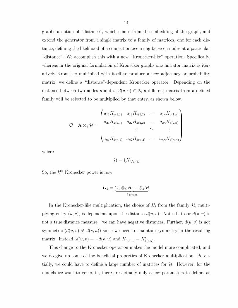
graphs a notion of “distance”, which comes from the embedding of the graph, and

extend the generator from a single matrix to a family of matrices, one for each dis-

tance, defining the likelihood of a connection occurring between nodes at a particular

“distance”. We accomplish this with a new “Kronecker-like” operation. Specifically,

whereas in the original formulation of Kronecker graphs one initiator matrix is iter-

atively Kronecker-multiplied with itself to produce a new adjacency or probability

matrix, we define a “distance”-dependent Kronecker operator. Depending on the

distance between two nodes u and v, d(u, v) ∈ Z, a different matrix from a defined

family will be selected to be multiplied by that entry, as shown below.

C =A⊗d H =

a11Hd(1,1) a12Hd(1,2) . . . a1nHd(1,n)

a21Hd(2,1) a22Hd(2,2) . . . a2nHd(2,n)

......

. . ....

an1Hd(n,1) an2Hd(n,2) . . . annHd(n,n)

where

H = {Hi}i∈Z

So, the kth Kronecker power is now

Gk = G1 ⊗d H · · ·⊗d H� �� �k times

In the Kronecker-like multiplication, the choice of Hi from the family H, multi-

plying entry (u, v), is dependent upon the distance d(u, v). Note that our d(u, v) is

not a true distance measure—we can have negative distances. Further, d(u, v) is not

symmetric (d(u, v) �= d(v, u)) since we need to maintain symmetry in the resulting

matrix. Instead, d(u, v) = −d(v, u) and Hd(u,v) = H �d(v,u).

This change to the Kronecker operation makes the model more complicated, and

we do give up some of the beneficial properties of Kronecker multiplication. Poten-

tially, we could have to define a large number of matrices for H. However, for the

models we want to generate, there are actually only a few parameters to define, as

15

d(i, j) and a simple function defines Hi for i > 1. The underlying reason for this

simplicity is that the local lattice structure is usually specified by H0 and H1, while

the global, distance-dependent probability of connection can usually be specified by

an Hi with a simple form. So, while we lose the benefits of true Kronecker mul-

tiplication, we gain generality and the ability to create many different lattices and

probability of long-range contacts. We note in passing that the generation of these

lattice structures is not possible with the original formulation of the Kronecker graph

model. For example, it is impossible to generate the Watts-Strogatz model with con-

ventional Kronecker graphs. However, it can be done with the current generalization.

This is illustrated in our examples below.

Example 1 (Original Kronecker Graph). The simplest example is that of the original

Kronecker graph formulation. For this case, the “distance” can be arbitrary, and the

family of matrices, H, is simply G1, the same G1 used in the original definition.

Thus, we define

Gk = G1 ⊗d H · · ·⊗d H� �� �k times

= G1 ⊗G1 ⊗ . . . G1� �� �k times

Example 2 (Watts-Strogatz Small-World Model). The next example we consider, the

Watts-Strogatz model, consists of a ring of n nodes, each connected to their neighbors

within distance k on the ring. The probability of a connection to any other node on

the ring is then P (u, v) = p [133]. To generate the underlying ring structure with

k = 1, start with an initiator matrix K1, representing the graph in Figure 2.1(a).

Figure 2.1: Generating the Watts-Strogatz model

In order to obtain the sequence of matrices representing the graphs in Figure 2.1,

we define a “distance” measure as the number of hops from one node to another along

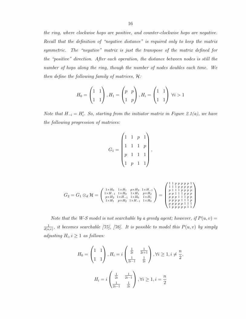
16

the ring, where clockwise hops are positive, and counter-clockwise hops are negative.

Recall that the definition of “negative distance” is required only to keep the matrix

symmetric. The “negative” matrix is just the transpose of the matrix defined for

the “positive” direction. After each operation, the distance between nodes is still the

number of hops along the ring, though the number of nodes doubles each time. We

then define the following family of matrices, H:

H0 =

1 1

1 1

, H1 =

p p

1 p

, Hi =

1 1

1 1

∀i > 1

Note that H−i = H �i. So, starting from the initiator matrix in Figure 2.1(a), we have

the following progression of matrices:

G1 =

1 1 p 1

1 1 1 p

p 1 1 1

1 p 1 1

,

G2 = G1 ⊗d H =

�1×H0 1×H1 p×H2 1×H−11×H−1 1×H0 1×H1 p×H2p×H2 1×H−1 1×H0 1×H11×H1 p×H2 1×H−1 1×H0

�=

1 1 p p p p p 11 1 1 p p p p p

p 1 1 1 p p p p

p p 1 1 1 p p p

p p p 1 1 1 p p

p p p p 1 1 1 p

p p p p p 1 1 11 p p p p p 1 1

Note that the W-S model is not searchable by a greedy agent; however, if P (u, v) =

1d(u,v) , it becomes searchable [75], [76]. It is possible to model this P (u, v) by simply

adjusting Hi, i ≥ 1 as follows:

H0 =

1 1

1 1

, Hi = i

12i

12i+1

12i−1

12i

, ∀i ≥ 1, i �= n

2,

Hi = i

12i

12i−1

12i−1

12i

, ∀i ≥ 1, i =n

2

17

As in the previous examples, H−i = H �i. The different definition for the middle node

in the ring is due to the fact that we need the probability of a connection to reach

a minimum at this point, and then start to rise again. With this new definition of

Hi, i ≥ 1, we have the following progression of matrices:

G1 =

1 1 1/2 1

1 1 1 1/2

1/2 1 1 1

1 1/2 1 1

,

G2 = G1 ⊗d H =

�1×H0 1×H1 1/2×H2 1×H−1

1×H−1 1×H0 1×H1 1/2×H2

1/2×H2 1×H−1 1×H0 1×H1

1×H1 1/2×H2 1×H−1 1×H0

�=

1 1 1/2 1/3 1/4 1/3 1/2 11 1 1 1/2 1/3 1/4 1/3 1/2

1/2 1 1 1 1/2 1/3 1/4 1/31/3 1/2 1 1 1 1/2 1/3 1/41/4 1/3 1/2 1 1 1 1/2 1/31/3 1/4 1/3 1/2 1 1 1 1/21/2 1/3 1/4 1/3 1/2 1 1 11 1/2 1/3 1/4 1/3 1/2 1 1

This example already illustrates that the generalized operator we have defined allows

the generation of searchable networks, but we will provide another more realistic ex-

ample in the next example.

Example 3 (Kleinberg-like Model). The final example we consider, Kleinberg’s lattice

model, is particularly pertinent as it was shown to be searchable [75]. In the original

formulation, local connections of nodes are defined on a k-dimensional lattice, and

long-range links occur between two nodes at distance d with probability proportional

to d−α. We focus on a “Kleinberg-like” model here, where instead of a k-dimensional

lattice, we have an “expanding hypercube” as our underlying lattice. In this example,

Figure 2.2: Example: the growth of an expanding hypercube

at any point, the graph is a hypercube with some extra long-range connections, and

when it grows, it grows by doubling the number of nodes and adding a dimension to

18

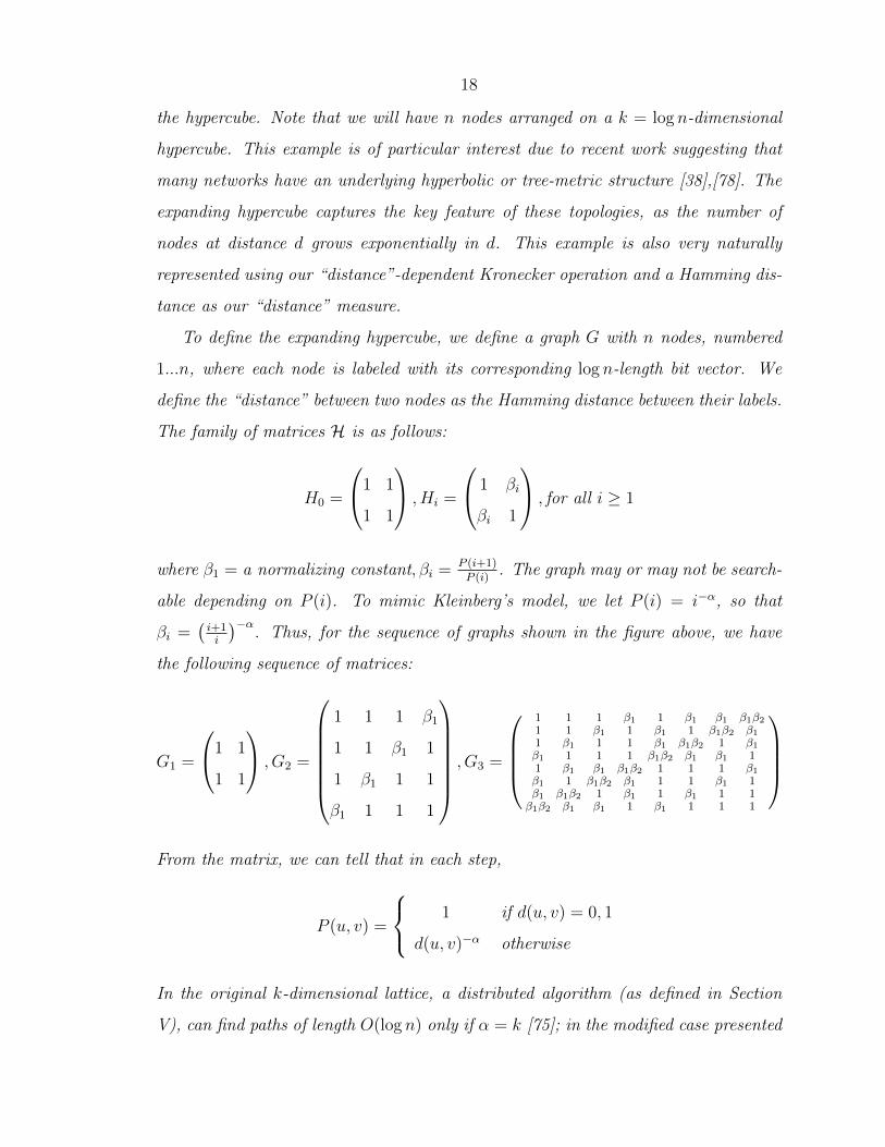
the hypercube. Note that we will have n nodes arranged on a k = log n-dimensional

hypercube. This example is of particular interest due to recent work suggesting that

many networks have an underlying hyperbolic or tree-metric structure [38],[78]. The

expanding hypercube captures the key feature of these topologies, as the number of

nodes at distance d grows exponentially in d. This example is also very naturally

represented using our “distance”-dependent Kronecker operation and a Hamming dis-

tance as our “distance” measure.

To define the expanding hypercube, we define a graph G with n nodes, numbered

1...n, where each node is labeled with its corresponding log n-length bit vector. We

define the “distance” between two nodes as the Hamming distance between their labels.

The family of matrices H is as follows:

H0 =

1 1

1 1

, Hi =

1 βi

βi 1

, for all i ≥ 1

where β1 = a normalizing constant, βi =P (i+1)P (i) . The graph may or may not be search-

able depending on P (i). To mimic Kleinberg’s model, we let P (i) = i−α, so that

βi =�i+1i

�−α

. Thus, for the sequence of graphs shown in the figure above, we have

the following sequence of matrices:

G1 =

1 1

1 1

, G2 =

1 1 1 β1

1 1 β1 1

1 β1 1 1

β1 1 1 1

, G3 =

1 1 1 β1 1 β1 β1 β1β21 1 β1 1 β1 1 β1β2 β11 β1 1 1 β1 β1β2 1 β1β1 1 1 1 β1β2 β1 β1 11 β1 β1 β1β2 1 1 1 β1β1 1 β1β2 β1 1 1 β1 1β1 β1β2 1 β1 1 β1 1 1

β1β2 β1 β1 1 β1 1 1 1

From the matrix, we can tell that in each step,

P (u, v) =

1 if d(u, v) = 0, 1

d(u, v)−α otherwise

In the original k-dimensional lattice, a distributed algorithm (as defined in Section

V), can find paths of length O(log n) only if α = k [75]; in the modified case presented

19

above, we will see in section V that we need a different probability of connection to

find short paths.

2.4 Connection to hidden hyperbolic space model

As mentioned previously, the expanding hypercube model in Example 3 resembles

models proposed in [5] and extended in [78], [22], and [23]. In [5], every node in

the network has a hidden variable — their location in a hidden metric space. The

probability of a connection between two nodes is based upon the distance between

them in this hidden space. The resulting degree distribution depends on the curvature

of this hidden space; if the space has negative curvature, the degree distribution will

be scale-free with P (k) = k−γ [79].

In the distance-dependent Kronecker graph described in this chapter and [16], the

probability of a connection is based on the distance between two nodes in the given

lattice, defined usually by H0 and H1 in the family of matrices H. As a result, the

lattice, or metric space, is not really hidden since neighbors are explicitly connected in

the lattice. It is important to note that both models incorporate a distance-dependent

probability of connection. As will be defined formally in Section 2.6, a local greedy

search algorithm can take advantage of this embedding into a hidden or physical

space to forward a message to a destination. If a given node u has a message to

forward to a destination t, it can use its knowledge of the embedding to forward the

message to its neighbor closest to the destination in the embedding. It is not necessary

that the embedding be physical, as shown in [78] and [22]; rather, what is necessary

is that the the probability of a connection between two nodes is dependent on the

distance between them. In most social networks the abstract distance is a measure

of “social distance” — the likelihood of two individuals being connected depends on

their memberships in various groups, among other factors.

In addition, in the models of [5], a hyperbolic space results in exponentially ex-

panding neighborhoods around each node. In the distance-dependent hypercube ex-

ample, there are�k

d

�nodes at each distance d, also resulting in exponentially expand-

20

ing neighborhoods. However, the hidden metric space model necessarily includes the

notion of a core and periphery of the network, where high-degree nodes form the core

connecting many low-degree nodes at the periphery [22]. In the hypercube example,

all nodes are homogeneous in expected degree — there is no notion of a core.

In [78], as nodes are located further from the origin in the hidden hyperbolic

space their expected degree decreases exponentially (∝ e−βr). When this is combined

with the exponentially expanding neighborhoods (∝ eαr), the result is a scale-free

distribution with γ = 1 + α

β. It is important to note that an exponential decrease

in expected degree is not strictly necessary; to see this, let the number of nodes at

distance r from a reference origin in the hyperbolic space be n(r) = eαr and let the

average degree of nodes at distance r be k(r) = r−δ, so that r(k) = k− 1δ . Using

n(k) ∝ n[r(k)] |r�(k)|, we have

n(k) ∝ eαk−1/δ

k−1/δ−1

which asymptotically behaves like a power law with γ = 1 + 1/δ. In the hypercube

example, despite the exponential expansion of neighborhoods, the resulting degree

distribution will always be Poisson as long as the probability of connection is suffi-

ciently small, as shown in the next section.

Nevertheless, the connection between this model and those based on tree metrics

and hidden metric spaces is important to note, as one key factor emerges: a distance-

dependent relation is necessary for a greedy algorithm to succeed in finding shortest

paths.

2.5 Degree distribution

In this section we describe a general characteristic function-based analysis of degree

distributions for lattice-based networks, and apply it to the expanding hypercube ex-

ample in Section 2.3. In general, any lattice-based network with a distance-dependent

probability of connection will have a Poisson degree distribution, as long as the prob-

21

ability of a connection at a distance d is sufficiently small. Formally,

Theorem 2.1. The degree distribution of a general lattice-based network with a

distance-dependent probability of connection P (d) and maximum distance dmax will

have the following degree distribution:

P (ν = i) =e−ααi

i!

�1 + dmaxO(P 2(d))

�

where

α =dmax�

d=1

P (d)σ(d) (2.1)

and σ(d) = number of nodes at distance d from a reference node in the lattice. We

note that if limn→∞ dmaxP 2(d) = 0, then the degree distribution is Poisson.

Proof. Let ν denote the degree of an arbitrary node u in a general lattice-based

network with n nodes. Thus, ν = v1 + v2 + · · ·+ vn where

vi =

1 if link to node i,

0 otherwise.

We define the characteristic function of the degree distribution as

E[eitν ] =E[eit(v1+v2+···+vn)] = E[eitv1 ]E[eitv2 ] . . . E[eitvn ]

We can then group the expectations

E[eitν ] =dmax�

d=1

(1− P (d) + P (d)eit)σ(d)

=dmax�

d=1

(1− P (d)(1− eit))σ(d)

=dmax�

d=1

�e−P (d)(1−e

it) +O(P 2(d))(1− eit)2�σ(d)

(2.2)

as e−x = 1 − x + O(x2). Thus, we can pull out the first term and using binomial

22

approximation of (1 + x)c = 1 + cx+O(x2), we have

E[eitν ] =dmax�

d=1

e−P (d)(1−eit)σ(d)

�1 +

O(P 2(d))(1− eit)2σ(d)

e−P (d)(1−eit)

�

= e−(1−eit)

�dmax

d=1 P (d)σ(d)dmax�

d=1

�1 +O(P 2(d))(1− eit)2σ(d)eP (d)(1−e

it)�

≈ eα(eit−1)(1 + dmaxO(P 2(d)))

Expanding, we see that the characteristic function is

E[eitν ] =�1 + dmaxO(P 2(d))

�e−α

�1 + αeit +

(αeit)2

2!+ . . .

�

From such a representation of the characteristic function, we can clearly see the degree

distribution as

P (ν = i) =e−ααi

i!

�1 + dmaxO(P 2(d))

�

We now turn to a specific lattice-based network, the hypercube distance-dependent

Kronecker graph described in Example 3 in Section 2.3. In this example, σ(d) =�k

d

�,

and the maximum distance in the network is k = log n. We use a particular P (d) =��

k− 2d3

d

3

�d log k ln 3

�−1

optimized for searchability, as determined in Section 2.6.

Theorem 2.2. The degree distribution of the expanding hypercube is given by the

following Poisson distribution,

P (ν = i) =e−ααi

i!where α ≈ 3.6919 n.4703

log log n√log n

(2.3)

Proof. We use the same framework as in the proof of Theorem 2.1, and let eit = x

for simplicity. In this case, the characteristic function becomes

E[xν ] = e−(1−x)�

k

d=1 P (d)σ(d)

23

so that

α =k�

d=1

P (d)σ(d) =k�

d=1

��k − 2d

3d

3

�d log k ln 3

�−1 �k

d

�

To calculate α, we use the entropy approximation�k

d

�≈ 2kH( d

k), which holds as

�n

k

�= 2n(H(p)+o(1)) when k ∝ pn, so that

α ≈ 1

log k ln 3

k�

d=1

d−12kH( d

k)−(k− 2d

3 )H�

d

3k− 2d

3

�

We can approximate the sum by using saddle point integration.

�g(y)ekf(y) dy =

�2π

k |f ��(y0)|g(y0)e

kf(y0)

�1 +O

�1√k

��(2.4)

where y0 is the saddle point of the function f(y), i.e., the point at which f �(y) = 0.

We rewrite the sum S(k) in nats, leaving out the constants in front,

S(k) =1

k

k�

d=1

k

dek

�H( d

k)−(1− 2d

3k)H�

d

3k1− 2d

3k

��

and then we let y = d

k,

S(y) =

� 1

1k

1

yek

�H(y)−(1− 2

3y )H�

y

31− 2

3y

��

dy

so that, with the saddle point approximation of line (4), g(y) = 1yand f(y) = H(y)−

(1− 23y )H(

y

3

1− 23y). Using Mathematica, we find

y0 = 0.417

f(y0) = 0.326

g(y0) = 2.4

|f ��(y0)| = 2.2

24

yielding,

S(k) ≈�

2π

2.2k(2.4)e0.326k (2.5)

So, our α is now

α ≈ 1

log k ln 3

�2π

2.2k(2.4)e0.326k ≈ 3.6919 n0.4703

log log n√log n

With the results of Theorem 2.1, we have a Poisson degree distribution with parameter

α.

2.5.1 Expected degree

From the characteristic function, we can also determine the expected degree.

E[ν] =∂

∂xE[xν ]

����x=1

=∂

∂x[e−(1−x)α]

����x=1

= α

Thus, the expected degree of the expanding hypercube example is a growing function

of n.

0 1000 2000 3000 4000 50005

10

15

20

25

30Expected Degree

n

Expec

tedDeg

ree,

over

50trials

SimulatedTheoretical

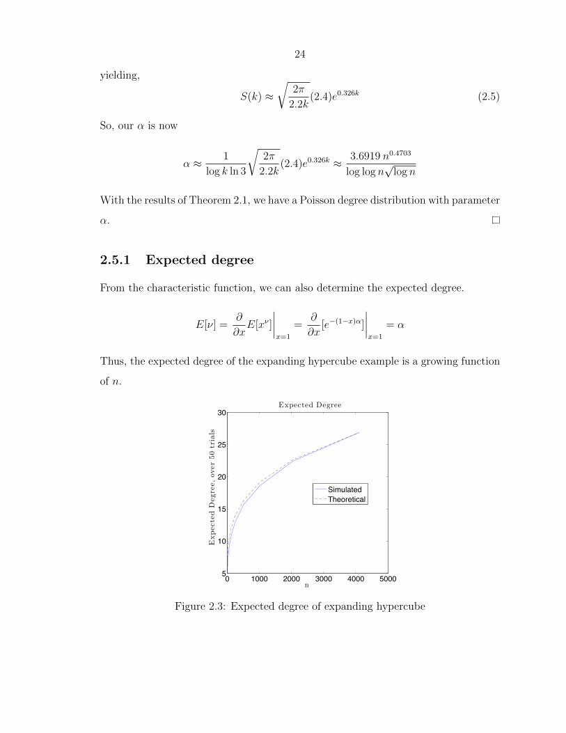
Figure 2.3: Expected degree of expanding hypercube

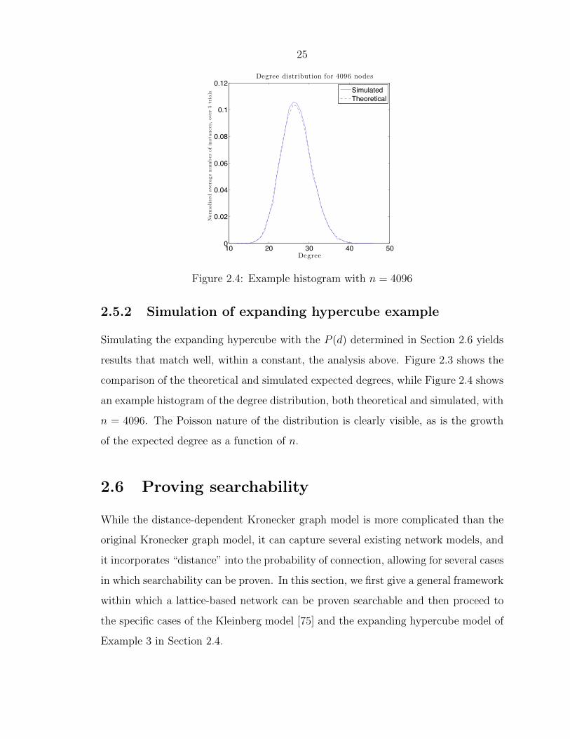
25

10 20 30 40 500

0.02

0.04

0.06

0.08

0.1

0.12Degree distribution for 4096 nodes

Degree

Norm

alize

dave

ragenumber

ofinstance

s,ove

r5trials

SimulatedTheoretical

Figure 2.4: Example histogram with n = 4096

2.5.2 Simulation of expanding hypercube example

Simulating the expanding hypercube with the P (d) determined in Section 2.6 yields

results that match well, within a constant, the analysis above. Figure 2.3 shows the

comparison of the theoretical and simulated expected degrees, while Figure 2.4 shows

an example histogram of the degree distribution, both theoretical and simulated, with

n = 4096. The Poisson nature of the distribution is clearly visible, as is the growth

of the expected degree as a function of n.

2.6 Proving searchability

While the distance-dependent Kronecker graph model is more complicated than the

original Kronecker graph model, it can capture several existing network models, and

it incorporates “distance” into the probability of connection, allowing for several cases

in which searchability can be proven. In this section, we first give a general framework

within which a lattice-based network can be proven searchable and then proceed to

the specific cases of the Kleinberg model [75] and the expanding hypercube model of

Example 3 in Section 2.4.

26

2.6.1 General searchability theorem

We define a decentralized algorithm A similar to [75]. In each step, the current

message-holder u passes the message to a neighbor that is closest to the destination,

t. Each node only has knowledge of its address on the lattice (given by its bit vector

label in the case of the expanding hypercube), the address of the destination, and

the nodes that have previously come into contact with the message. For the graph to

be searchable, we need to have that the distributed algorithm A is able to find short

paths through the network, which are usually O(D) where D is the diameter of the

network.

Let the current message-holder be node u and the destination node t. We will

say that the execution of a decentralized search algorithm A is in phase j when

2j < d(u, t) ≤ 2j+1, where d(u, t) is the distance between node u and node t. Thus,

the largest value of j in a general lattice-based network is jmax = log dmax where

dmax denotes the maximum geodesic in the network. For example, in a hypercube,

the maximum geodesic is dmax = log n = k, so jmax = log log n = log k. We define

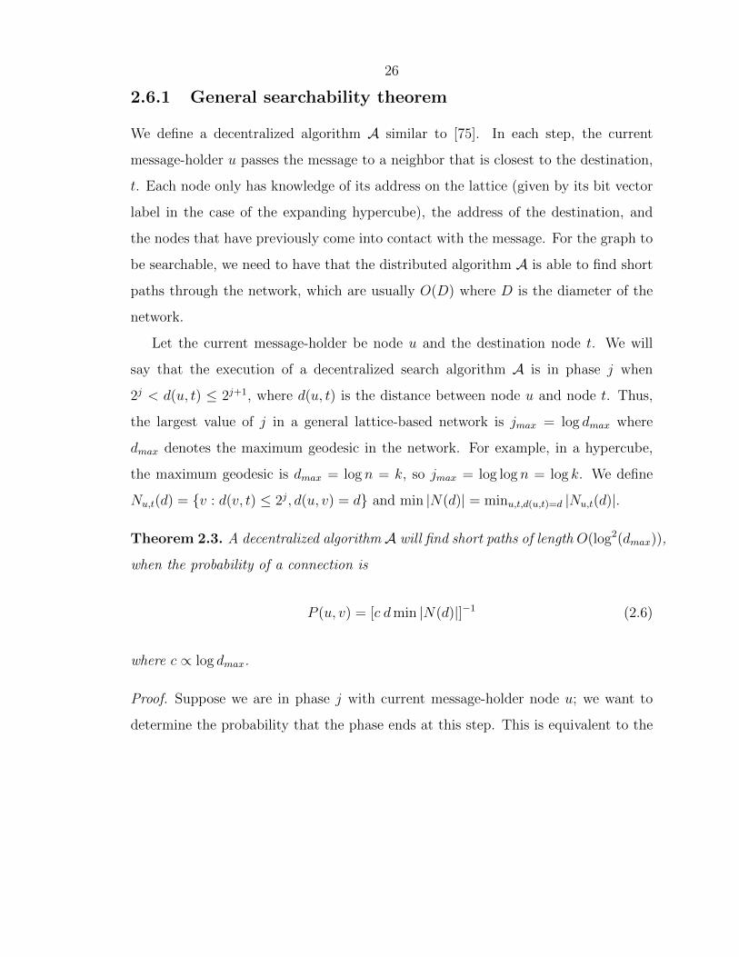
Nu,t(d) = {v : d(v, t) ≤ 2j, d(u, v) = d} and min |N(d)| = minu,t,d(u,t)=d |Nu,t(d)|.

Theorem 2.3. A decentralized algorithm A will find short paths of length O(log2(dmax)),

when the probability of a connection is

P (u, v) = [c dmin |N(d)|]−1 (2.6)

where c ∝ log dmax.

Proof. Suppose we are in phase j with current message-holder node u; we want to

determine the probability that the phase ends at this step. This is equivalent to the

27

probability that the message enters a set of nodes Bj where Bj = {v : d(v, t) ≤ 2j}.

Pr({message enters Bj}) =1−�

v∈Bj

(1− P (u, v : v ∈ Bj))

=1−d(u,t)+2j�

d=d(u,t)−2j

(1− P (d))|Nu,t(d)|

≥1−d(u,t)+2j�

d=d(u,t)−2j

(1− P (d))min|N(d)|

Figure 2.5: Relative positions of nodes u,v, and t in phase j

In any network model, enforcing searchability boils down to determining this

min |N(d)|, the minimum number of nodes at a distance d from a given node u within

a ball of nodes centered around the destination, t, as illustrated in Figure 2.5. Once

this min |N(d)| is found, if we set the probability of a connection between two nodes

distance d apart as in Theorem 2.3, with an appropriate constant, we will find that

each phase described above will end in approximately jmax steps, and, as there are

only jmax such phases, our greedy forwarding algorithm will be able to find very short

paths of length O(j2max

).

28

Thus, we have

Pr({message enters Bj}) ≥ 1−d(u,t)+2j�

d=d(u,t)−2j

(1− P (d))min|N(d)|

≈ 1− e−

�d(u,t)+2j

d=d(u,t)−2jmin|N(d)|P (d)

(2.7)

= 1− e− 1

c

�d(u,t)+2j

d=d(u,t)−2jd−1

≥ 1− e− 1

cln d(u,t)+2j

d(u,t)−2j

≥ 1− e−1cln 3 2j

2j

= 1− e−1c�

≥ 1

c�(2.8)

where the approximation in (2.7) requires that limn→∞ dmaxP 2(d) = 0, which holds

with the P (d) as specified in (2.6) (see proof of Theorem 2.1 for extra order terms),

and (2.8) comes from the power series expansion of e−x. Let Xj denote the total

number of steps spent in phase j. Then,

EXj =∞�

i=1

Pr[Xj ≥ i] ≤∞�

i=1

�1− 1

c�

�i−1

= c�

Let X denote the total number of steps taken by the algorithm A.

X =jmax�

j=0

Xj

and

EX =jmax�

j=0

EXj ≤ (1 + jmax)(c�) = (1 + log dmax) log dmax ≤ δ(log dmax)

2

where the last bound holds ∀ δ ≥ 2, log dmax ≥ 2.

With this framework, we can explore the searchability of any lattice-based network

model with distance-dependent connection probability.

29

2.6.2 Searchability in original Kleinberg model

In the original Kleinberg two-dimensional lattice [75], the number of nodes at a

distance d from a reference node is approximately 4d, ignoring edge effects. The

maximum distance between any two nodes is O(n), so jmax ≈ log n. Addition-

ally, the diameter of the graph is on the order of log n. In general, min |N(d)| ∝ d

for a fixed j, resulting in the probability of connection optimized for searchability,

P (d) = [α log(n)d2]−1. Using this P (d),

Pr({message enters Bj}) ≥ 1−d(u,t)+2j�

d=d(u,t)−2j

(1− P (d))min|N(d)|

≈ 1− e− 1

α logn

�d(u,t)+2j

d=d(u,t)−2jd−1

(2.9)

≥ 1− e−1

α� logn

≥ 1

α� log n(2.10)

where (2.9) holds for the P (d) specified, and (2.10) comes from the power series

expansion of e−x. Therefore,

EXj ≤ α� log n

and

EX =logn�

j=0

EXj ≤ δ(log n)2.

where the bound above holds ∀ δ ≥ 2, log n ≥ 2.

2.6.3 Searchability in expanding hypercube example

In the expanding hypercube example of Section 2.3, each node has log n neighbors

from the lattice itself. With the addition of long-range links, we expect the diameter to

be O(log log n), similar to [78]. Note that with this example, jmax = log log n = log k

and the number of nodes at distance d equals�n

d

�. Using Theorem 2.3, we can prove

the following result:

30

Theorem 2.4. A decentralized algorithm A will find paths of length O((log log n)2)

in the expanding hypercube example when

β0 =1, β1 = [2 log k ln 3]−1 ,

βi =

��k − 2i

3i

3

�i

� ��k − 2(i+1)

3i+13

�(i+ 1)

�−1

∀i ≥ 2 (2.11)

such that the probability of a connection is

P (u, v) =

1 if d(u, v) = 0, 1��

k− 2d3

d

3

�d log k ln 3

�−1

if d(u, v) = d(2.12)

Proof. Using Theorem 2.3, all that remains is to find min |N(d)| and to determine

the appropriate constants to use. Without loss of generality, we assume that the

destination node t is the all-zero node (i.e., its label is the zero vector) so that we can

write d(u, t) = �u�. To determine min |N(d)| in our case, since the distance measure

is a Hamming distance, we must count the number of possible bit vectors that are at

a specific distance d from a node u while still being within a certain distance of the

destination. We prove that min |N(d)| =�k− 2d

3d

3

�in 2.9. We then let c = log k ln 3 for

reasons that will be clear below. Using the same framework as in Theorem 2.3 we

have that

Pr({msg enters Bj}) ≥ 1−�u�+2j�

d=�u�−2j

(1− P (d))min|N(d)|

≈ 1− e− 1

log k ln 3

��u�+2j

d=�u�−2jd−1

(2.13)

≥ 1− e−1

log k

≥ 1

log k(2.14)

where (2.13) holds for the P (d) specified, and (2.14) comes from the power series

31

expansion of e−x. Therefore, we have

EXj ≤ log k

and

EX =log k�

j=0

EXj ≤ δ(log k)2, ∀ δ ≥ 2, log k ≥ 2

Since the expected number of steps in phase j is log k, and there are at most log k

phases, the expected amount of steps taken by the algorithm A is at most δ log2 k.

So, with this definition of P (d), the distributed algorithm provides searchability.

2.6.4 Simulation of distributed search algorithm

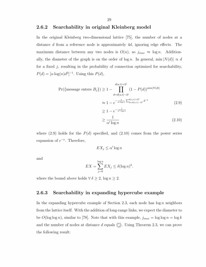
We simulated the local greedy algorithm described above in MATLAB for 16 ≤n ≤ 4096 with the probability distribution as in Theorem 2.4 and appropriate floor

functions. We found that the greedy algorithm finds a path between two nodes with an

average length of a constant factor away from the diameter of the simulated network,

where diameter is defined as the maximum geodesic in the network. Note that the two

nodes selected for the simulation are actually the “worst-case” nodes - the distance

between them in the network is exactly the diameter. Figure 2.6 illustrates the results

of the greedy algorithm simulations.

2.6.5 Path length with suboptimal P(d)

In this section we analyze the performance of the local greedy search algorithm on

the expanding hypercube when P (d) is not optimal, as in Theorem 2.4. For this

example, let P (d) = [log k�k

d

�]−1, which is clearly not min |N(d)| from Lemma 2.5.

We will show that this suboptimal P (d) also allows for searchability.

32

0 1000 2000 3000 4000 50002

2.5

3

3.5

4

4.5

5

5.5Average diameter and path length of simulated ddKron graphs

n

Averagediameter

and

path

length

,over

20trials

Simulated diameterPath length found by dist alg

Figure 2.6: Average path length found by greedy algorithm using local information

Using the same framework as in Theorem 2.3,

Pr({msg enters Bj}) ≥ 1−d(u,t)+2j�

d=d(u,t)−2j

(1− P (d))min|N(d)|

≈ 1− e�d(u,t)+2j

d=d(u,t)−2jP (d)min|N(d)|

(2.15)

= 1− e−

�d(u,t)+2j

d=d(u,t)−2jP (d)(

k− 2d3

d

3)

= 1− e−1

log kS(k,d)

≥ 1− e−1

log kminS(k,d)

where line (2.15) holds for the specified P (d) and where

S(k, d) =3∗2j�

d=2j

�k

d

�−1�k − 2d3

d

3

�

≈3∗2j�

d=2j

2(k− 2d

3 )H(d

3k− 2d

3)−kH( d

k)

(2.16)

≥ mind

3∗2j�

d=2j

2(k− 2d

3 )H(d

3k− 2d

3)−kH( d

k)

≥ 2maxd (k− 2d

3 )H(d

3k− 2d

3)−kH( d

k)

33

where we have used the approximation�k

d

�≈ 2kH( d

k), which holds as

�n

k

�= 2n(H(p)+o(1))

when k ∝ pn, in line (2.16). Since the exponent is convex in d, the maximum will be

at either the upper or lower bound of the sum. For 0 ≤ j ≤ log k the lower bound

(d = 2j) yields the maximal exponent. So, we have

Pr({msg enters Bj}) ≥1− e−1

log k2f(k,j) ≥ 2f(k,j)

log k

where we have used the power series expansion of e−x and where

f(k, j) = (k − 2j+1

3)H(

2j

3

k − 2j+1

3

)− kH(2j

k). (2.17)

Continuing with the proof of searchability, we have

EXj =∞�

i=1

Pr[Xj ≥ i] ≤ log k 2−f(k,j)

and

EX =log k�

j=0

EXj ≤ (1 + log k) log k 2−minj f(k,j) ≤ δ(log k)2, ∀ δ ≥ 2, log k ≥ 2

since f(k, j) is convex but its minimum occurs close to log k. As a result, even

for suboptimal P (d), a local greedy algorithm can find short paths. However, the

bounds used in the analysis above are looser than those in previous sections, so the

final expected number of steps taken by A is not as tight. This analysis is supported

by simulation results as shown in the figure below. Finally, if P (d) = [d log k�k

d

�]−1,

using the same sort of techniques as above we can show that EX ≤ δk(log k)2 for

a large enough δ. Note that in this case, the paths found will be O(log n log log n),

which are longer than before. Simulation results with this P (d) are shown in Figure

2.8.

34

0 500 1000 1500 2000 25001

1.5

2

2.5

3

3.5

4

4.5

5Average diameter and path length of simulated ddKron graphs with suboptimal P (d)

n

Averagediameter

andpath

length

,over

20trials

Simulated diameterPath length found by dist alg

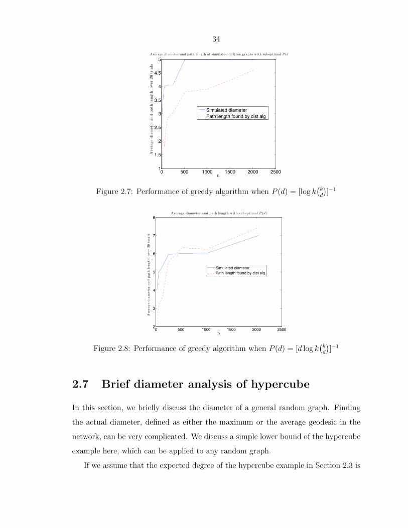
Figure 2.7: Performance of greedy algorithm when P (d) = [log k�k

d

�]−1

0 500 1000 1500 2000 25002

3

4

5

6

7

8Average diameter and path length with suboptimal P (d)

n

Ave

ragediameter

andpath

length

,ove

r20trials

Simulated diameterPath length found by dist alg

Figure 2.8: Performance of greedy algorithm when P (d) = [d log k�k

d

�]−1

2.7 Brief diameter analysis of hypercube

In this section, we briefly discuss the diameter of a general random graph. Finding

the actual diameter, defined as either the maximum or the average geodesic in the

network, can be very complicated. We discuss a simple lower bound of the hypercube

example here, which can be applied to any random graph.

If we assume that the expected degree of the hypercube example in Section 2.3 is

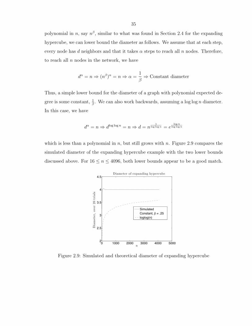
35

polynomial in n, say nβ, similar to what was found in Section 2.4 for the expanding

hypercube, we can lower bound the diameter as follows. We assume that at each step,

every node has d neighbors and that it takes α steps to reach all n nodes. Therefore,

to reach all n nodes in the network, we have

dα = n ⇒ (nβ)α = n ⇒ α =1

β⇒ Constant diameter

Thus, a simple lower bound for the diameter of a graph with polynomial expected de-

gree is some constant, 1β. We can also work backwards, assuming a log log n diameter.

In this case, we have

dα = n ⇒ dlog logn = n ⇒ d = n1

log logn = elogn

log logn

which is less than a polynomial in n, but still grows with n. Figure 2.9 compares the

simulated diameter of the expanding hypercube example with the two lower bounds

discussed above. For 16 ≤ n ≤ 4096, both lower bounds appear to be a good match.

0 1000 2000 3000 4000 50002

2.5

3

3.5

4

4.5Diameter of expanding hypercube

n

Diameter,ov

er20trials

SimulatedConstant, ! = .25loglog(n)

Figure 2.9: Simulated and theoretical diameter of expanding hypercube

36

2.8 Conclusion

We have presented a generalization of Kronecker graphs by defining a family of

“distance”-dependent matrices and a new Kronecker-like operation. As a result, the

network model defines both local regular structures and global distance-dependent

connections. Though the model is more complicated than the original Kronecker

graph model, it is more general, as it can generate existing social network models, and

more importantly, networks that are searchable. These properties emerge naturally

from the definition of the embedding of the nodes and the probability of connection

within the family of matrices H. Any lattice-based network model with distance-

dependent connection probabilities can be analyzed using the framework described

in Sections 2.5, 2.6, and 2.7 for exploring degree distribution, diameter, and searcha-

bility. Most importantly, the searchability analysis shows how to make any network

model searchable by defining the appropriate probability of connection based upon

|N(d)|. The particular expanding hypercube example explicitly described here shares

characteristics with those based upon hidden hyperbolic spaces [5], [78], though it

has one major difference — degree homogeneity across nodes. Nevertheless, its expo-

nentially expanding neighborhoods and distance-dependent probability of connection

make it a good model for social networks as people tend to exhibit strong homophily,

i.e., associating with other people most like themselves. In addition, in contrast to

Kleinberg’s lattice-based model [75], the searchability of the expanding hypercube is

not too sensitive to the choice of P (d).

Though this chapter gives a near complete description of the characteristics of

“distance”-dependent Kronecker graphs, there are many interesting questions that

remain. These include how to parameterize the model from real-world data sets, and

how to incorporate network dynamics. Ideally, given any data set, we would like

to be able to find an appropriate family of distance-dependent matrices to match

any desired characteristic of the data set. Additionally, while the current model

incorporates some measure of growth, growing from a small initiator matrix to a final

nxn adjacency matrix, we would like to better incorporate mobility into the model

37

so that it is not just a static description of the network at one point in time.

2.9 Appendix: Calculating the size of Nu,t(d)

In this section, we show a lower bound for |Nu,t(d)|, the number of nodes at distance

d from a given node u, still within distance 2j of the destination, t.

Lemma 2.5. min |Nu,t(d)| =�k− 2d

3d

3

�

Proof. We first count exactly the number of nodes in Nu,t(d), the number of nodes

at a distance d from a given node u within a ball of nodes centered around the

destination, t, as illustrated in Figure 2.5. Without loss of generality, define t as the

all-zero node, t = (00...0). Arrange the label of u such that u = (1 ... 1 0... 0). Define

v = (v11 v10 v01 v00) according to this partition of u, so that v11 and v01 have “1”

entries and v10 and v00 have “0” entries. Let �x� denote the weight, or number of

ones, of the label of node x. We know the following:

v11 + v10 + v01 + v00 = k

v11 + v10 = �u�

v01 + v10 = d

v11 + v01 = �v�

We can solve in terms of v11, yielding

v00 =k − d− v11

v10 = �u� − v11

v01 =d− �u�+ v11

38

We also know that we must satisfy the following:

v11, v10, v01, v00 ≥ 0

2j < �u� ≤ 2j+1

�u� − 2j ≤ d ≤ �u�+ 2j

�v� ≤ 2j

From these bounds we have

max(0, �u� − d) ≤ v11 ≤ min(�u� , k − d,1

2(2j + �u� − d))

Note that the second and third bounds do not affect v11. Counting the number of

nodes in the ball, we have

|Nu,t(d)| =vu�

v11=vl

��u�v11

��k − �u�

d− �u�+ v11

�

where we have substituted vu and vl, for the upper and lower bounds above, respec-

tively. We can now approximate the number of nodes in Nu,t(d), using the entropy

approximation for combinations. Let �u� = ak, d = bk, 2j = ck, x = v11. Using this

notation, we have

|Nu,t(d)| =vu�

x=vl

�ak

x

��k(1− a)

k(1− b) + x

�

≈vu�

x=vl

2k(aH( x

ak)+(1−a)H

�b−a+x

k

1−a

�)

(2.18)

≥2kX

where

X = maxx

aH� x

ak

�+ (1− a)H

�b− a+ x

k

1− a

�(2.19)

39

subject to

kmax(0, a− b) ≤ x ≤ kmin(a, 1− b,1

2(a− b+ c))

Note that (2.18) is true as�n

k

�= 2n(H(p)+o(1)) when k ∝ pn.

Note that the function X is concave in x, so unconstrained optimization yields

the two solutions below, each giving different values of min |Nu,t(d)|:

x∗1 = ak − abk when c ≥ a+ b(1− 2a), yielding min |Nu,t(d)| =

�k

d

�

x∗2 =

1

2k(a− b+ c) when c < a+ b(1− 2a), yielding min |Nu,t(d)| =

�k − 2d

3d

3

�

The resulting min |Nu,t(d)| are derived in Sections 2.9.1 and 2.9.2. As the second

solution yields a smaller min |Nu,t(d)|, we have an overall min |Nu,t(d)| =�k− 2d

3d

3

�.

2.9.1 Solution 1: c ≥ a+ b(1− 2a)

In this region, the solution to the unconstrained problem, x∗1 = ak − abk gives us

the maximal X . Substituting in for the size of Nu,t(d) and using the same entropy

approximation as before, we have

|Nu,t(d)| = 2k(aH(ak−abk

ak)+(1−a)H

�b−a+ak−abk

k

1−a

�)

= 2k(aH(1−b)+(1−a)H(b)) = 2kH(b) ≈�k

bk

�=

�k

d

�.

2.9.2 Solution 2: c < a+ b(1− 2a)

In this region, we choose one of the boundary points, x∗2 = 1

2k(a − b + c), as the

solution to the maximization problem. Substituting this solution for x in |Nu,t(d)|,we obtain

|Nu,t(d)| = 2k(aH(a−b+c

2a )+(1−a)H(−a+b+c

2(1−a) ))

40

This gives us a function of a, b, c, so we want to find the worst case a, c that minimizes

|Nu,t(d)|. The new optimization problem is thus

f(b) =min |Nu,t(d)|

=mina,c

aH

�a− b+ c

2a

�+ (1− a)H

�−a+ b+ c

2(1− a)

�(2.20)

Note that the bounds for this region are:

1. a− b− c ≤ 0

2. a− b+ c ≥ 0

3. c < a ≤ 2c

4. 0 ≤ c ≤ 12

5. 0 ≤ a, b ≤ 1

6. 0 ≤ 2− a− b− c

7. 0 ≤ a+ b− c

8. 0 ≤ a+ b− c− 2ab

where 1 and 2 come from the bounds on d(u, v), 3 comes from the bounds on �u�,and 4 and 5 come from the ranges for j and the size of the network. Note that 1–5 are

always true, not just in this region. 6, 7, and 8 come from the fact that our solution

x∗2 is minimal in this region. Note that 8 implies 7.

Computing the Hessian of the function in (2.20) shows that it is concave in both

a and b; the derivation is in 2.9.3. Since our function is concave, the min |Nu,t(d)| isfound from the boundary points of Region 2. Rearranging the bounds from before in

terms of a we have:

1. a ≤ b+ c

2. a ≥ b− c

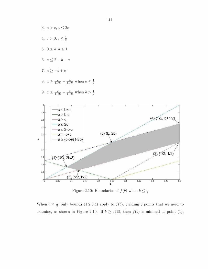
41

3. a > c, a ≤ 2c

4. c > 0, c ≤ 12

5. 0 ≤ a, a ≤ 1

6. a ≤ 2− b− c

7. a ≥ −b+ c

8. a ≥ c

1−2b −b

1−2b when b ≤ 12

9. a ≤ c

1−2b −b

1−2b when b > 12

Figure 2.10: Boundaries of f(b) when b ≤ 12

When b ≤ 12 , only bounds (1,2,3,4) apply to f(b), yielding 5 points that we need to

examine, as shown in Figure 2.10. If b ≥ .115, then f(b) is minimal at point (1),

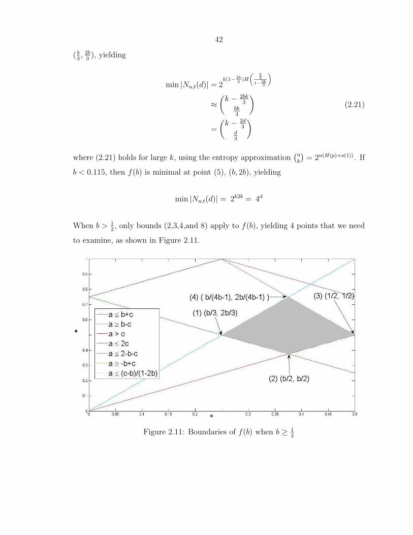
42

( b3 ,2b3 ), yielding

min |Nu,t(d)| = 2k(1− 2b

3 )H

�b

31− 2b

3

�

≈�k − 2bk

3bk

3

�(2.21)

=

�k − 2d

3d

3

�

where (2.21) holds for large k, using the entropy approximation�n

k

�= 2n(H(p)+o(1)). If

b < 0.115, then f(b) is minimal at point (5), (b, 2b), yielding

min |Nu,t(d)| = 2k2b = 4d

When b > 12 , only bounds (2,3,4,and 8) apply to f(b), yielding 4 points that we need

to examine, as shown in Figure 2.11.

Figure 2.11: Boundaries of f(b) when b ≥ 12

43

For this region, f(b) is minimal at point (1), matching point (5) in the previous

region, yielding

min |Nu,t(d)| = 2k(1− 2b

3 )H

�b

31− 2b

3

�

≈�k − 2d

3d

3

�(2.22)

where (2.22) holds for large k, using the entropy approximation�n

k

�= 2n(H(p)+o(1)).

Thus, when b < 0.115, we have min |Nu,t(d)| = 4d, and when b ≥ 0.115, we have

min |Nu,t(d)| =�k− 2d

3d

3

�. Finally, we have that when c < a + b(1 − 2a), we apply

Solution 2, and we have min |Nu,t(d)| =�k− 2d

3d

3

�when Solution 2 is valid. Comparing

the Solution 1 with Solution 2, we have again that min |Nu,t(d)| =�k− 2d

3d

3

�.

2.9.3 Concavity of f(a, b, c) for Solution 2

Lemma 2.6. The function f(a, b, c) = aH�a−b+c

2a

�+ (1 − a)H

�−a+b+c

2(1−a)

�is concave

in both a and b.

Proof. To prove that the function is concave in both a and b, we need to see if the

Hessian is negative definite. Let

f(a, b, c) = aH

�a− b+ c

2a

�+ (1− a)H

�−a+ b+ c

2(1− a)

�

Taking derivatives with respect to a, we find

∂f

∂a=

1

2

�− log

c+ a− b

2a− log

b+ a− c

2a+ log

c− a+ b

2(1− a)+ log

2− a− b− c

2(1− a)

�

and

∂2f

∂a2=

−(c− b)2

a(c+ a− b)(b+ a− c)+

−(1− c− b)2

(1− a)(c− a+ b)(2− a− b− c)

=1

2

�−1

a− b+ c+

−1

a+ b− c+

2

a+

−1

−a+ b+ c+

−1

2− a− b− c+

2

1− a

�

44

From the bounds for this region, we can see that the function is concave in a. Taking

derivatives with respect to c, we find

∂f

∂c=

1

2(− log (c+ a− b) + log (a+ b− c)− log (c− a+ b) + log (2− a− b− c))

and∂2f

∂c2=

1

2

�−1

c+ a− b+

−1

a+ b− c+

−1

c− a+ b+

−1

2− a− b− c

�

From the bounds in this region, we can see that the function is concave in c. Taking

derivatives with respect to both a and c, we find

∂2f

∂c∂a=

1

2

�−1

a− b+ c+

1

a+ b− c+

1

−a+ b+ c+

−1

2− a− b− c

�

The Hessian H is

∂2

∂a2∂2

∂a∂c

∂2

∂a∂c

∂2

∂c2

We want to show that the Hessian is negative definite, i.e, that H < 0. We have

already shown that ∂2

∂a2< 0, so it remains to show that the second leading principal

minor of H is positive definite. This is just the determinant of H

det[H] =∂2

∂a2∂2

∂c2−

�∂2

∂a∂c

�2

> 0

We rewrite the second derivatives as

∂2

∂a2=

1

2

�f1 + f2 +

2

a+

2

1− a

�

∂2

∂c2=

1

2(f1 + f2)

∂2

∂a∂c=

1

2(f1 − f2)

45

where, from above,

f1 =−1

a− b+ c+

−1

2− a− b− c< 0

f2 =−1

a+ b− c+

−1

−a+ b+ c< 0

So, our determinant is now

det[H] =

�f1 + f2 +

2

a+

2

1− a

�(f1 + f2)− (f1 − f2)

2

=1

4(f1 + f2)

2 +1

4

�2

a+

2

1− a

�(f1 + f2)−

1

4(f1 − f2)

2

= f1f2 +(f1 + f2)

2a(1− a)

Simplifying, this is just

det[H] = −(−a−b+c+2ab)2[(a−b+c)(−2+a+b+c)(a+b−c)(a−b−c)a(a−1)]−1

which, from our bounds, is positive. Since the determinant of H is positive, and since

∂2

∂a2is negative, we can say that H is negative definite, and the function is concave in

both a and c.

46

Chapter 3

Matching

3.1 Introduction

Many-to-one matching markets exist in numerous different forms, such as college

admissions, matching medical interns to hospitals for residencies, assigning housing

to college students, and the classic firms and workers market. These markets are

widely studied in academia and also widely deployed in practice, and have been

applied to other areas, such as FCC spectrum allocation and supply chain networks

[9, 98]

In the conventional formulation, matching markets consist of two sets of agents,

such as medical interns and hospitals, each of which have preferences over the agents to

which they are matched. In such settings it is important that matchings are ‘stable’

in the sense that agents do not have incentive to change assignments after being

matched. The seminal paper on matching markets was by Gale and Shapley [54], and

following this work an enormous literature has grown, e.g., [77, 114, 115, 116] and

the references therein. Further, variations on Gale and Shapley’s original algorithm

for finding a stable matching are in use today by the National Resident Matching

Program (NRMP), which matches medical school graduates to residency positions at

hospitals [113].

However, as often happens when translating theory to reality, problems arise when

implementing the matching algorithms in the real world. For example, couples partic-

ipating in the NRMP would often reject their matches and search outside the system,

47

so much so that eventually a separate couples matching market was set up to fix

the problem. In housing assignment markets where college students are asked to list

their preferences over housing options, there is often collusion among friends to list

the same preference order for houses, in an attempt to be matched together. These

two examples highlight that ‘peer effects’, whether just between two people or a more

general set of friends, often play a significant role in many-to-one matchings. That

is, agents care not only where they are matched, but also which other agents are

matched to the same place. Similarly, ‘complementarities’ often play a role on the

other side of the market. For example, hospitals and colleges care not only about

which individual students are assigned to them, but also that the group has a certain

diversity, e.g., of specializations, gender, etc.

As a result of the issues highlighted above, there is a growing literature studying

many-to-one matchings with externalities (i.e., peer effects and complementarities)

[43, 58, 73, 74, 106, 110, 8, 44, 120] and the research has found that designing match-

ing mechanisms is significantly more challenging when externalities are considered,

e.g. incentive compatible mechanism design is no longer possible. In fact, even de-

termining the existence of stable matchings in the presence of externalities has been

difficult.

The reason for the difficulty is that there is no longer a guarantee that a sta-

ble many-to-one matching will exist when agents care about more than their own

matching [113, 115], and, if a stable matching does exist, it can be computation-

ally difficult to find [112]. Consequently, most research has focused on identifying

when stable matchings do and do not exist. Papers have proceeded by constrain-

ing the matching problem through restrictions of the possible preference orderings,

[43, 58, 73, 74, 106, 110], and by considered variations on the standard notion of

stability [8, 44, 120]. Our work also considers a modification of the model, described

in the following.

The key idea is that peer effects are often the result of an underlying social network.

That is, when agents care about where other agents are matched, it is often because

they are friends. With this in mind, we construct a model in Section 3.2 that includes

48

a weighted, undirected social network graph and allows agents to have utility functions

(which implicitly define their preference ordering) that depend on where neighbors

in the graph are assigned. The model is motivated by [8], which also considers peer

effects defined by a social network but focuses on one-sided matching markets rather

than two-sided matching markets.

We focus on two-sided exchange stable matchings — see Section 3.2 for a detailed

definition and a discussion for how this definition of stability differs from the tradi-

tional one in [54]. We note that this is a distinct notion of stability, but one that is

relevant to many situations where agents can compare notes with each other, such

as the housing assignment or medical matching problem. For example, in [8, 9, 50],

“pairwise-stability” is considered since they consider models where agents exchange

offices or licenses in FCC spectrum auctions. Further, consider a situation where two

hospital interns prefer to exchange the hospitals allocated to them by the NRMP. If

this is a traditional stable matching, the hospitals would not allow the swap, even

though the interns are highly unsatisfied with the match. Such a situation has been

documented in [66], and has led to a similar type of stability, exchange stability, as

defined in [2, 30, 31, 66]. Our definition of stability incorporates both sides of the

market, but considers only pairwise exchanges of agents.

Given our model of peer effects, the focus of the chapter is then on characterizing

the set of two-sided exchange stable matchings. Our results concern (i) the existence

of two-sided exchange stable matchings, (ii) algorithms for finding two-sided exchange

stable matchings, and (iii) the efficiency of exchange stable matchings (in terms of

social welfare).

With respect to the existence of stable matchings (Section 3.3), it is not difficult

to show using a potential function argument that in our model two-sided exchange

stable matchings always exist. Further, if students value houses according to the

same rules, the matching that maximizes social welfare is guaranteed to be two-sided

exchange stable. In fact, in this special case, the potential function of the game is

exactly the social welfare function. Given the contrast to the negative results that

are common for many-to-one matchings, e.g., [44, 112, 113], these results are perhaps

49

surprising. Upon closer examination, it becomes clear that the key ingredient for

the existence of stable matchings is network symmetry — the social network must

be undirected, as is required for many of the existence results in hedonic coalition

formation [7, 21, 28], a related market.

Further, due to the similarity of the potential and social welfare functions, the re-

sults on characterizing the existence of stable matchings naturally suggest two simple

algorithms for finding stable matchings, which we discuss in Section 3.4. To measure

the performance of these algorithms, we look at two sample social networks: (1) a

real-world social network among undergraduate students at the California Institute

of Technology and (2) an on-line social network generated from voting patterns of

Wikipedia members.

With respect to the efficiency of exchange stable matchings (Section 3.5), results

are not as easy to obtain. In this context, we limit our focus to one-sided matching

markets, but as a result we are able to attain bounds on the ratio of the welfare of

the optimal matching to that of the worst stable matching, i.e., the ‘price of anarchy’.

In certain cases, we can show that the ratio of the welfare of the optimal matching

to that of the best stable matching, i.e., the ‘price of stability’ is one. We can further

show that the bound on the price of anarchy is tight. When considering only one-

sided markets, our model becomes similar to hedonic coalition formation, but with

several key differences, as highlighted in Section 3.5. Our results (Theorems 3.5 and

3.6) show that the price of anarchy does not depend on the number of, say, interns,

but does grow with the number of, say, hospitals — though the growth is typically

sublinear. Further, we observe that the impact of the structure of the social network

on the price of anarchy happens only through the clustering of the network, which

is well understood in the context of social networks, e.g., [67, 131]. Finally, it turns

out that the price of anarchy has a dual interpretation in our context; in addition to

providing a bound on the inefficiency caused by enforcing exchange stability, it turns

out to also provide a bound on the loss of efficiency due to peer effects.

50

3.2 Model and notation

To begin, we define the model we use to study many-to-one matchings with peer

effects and complementarities. There are four components to the model, which we

describe in turn: (i) basic notation for discussing matchings; (ii) the model for agent

utilities, which captures both peer effects and complementarities; (iii) the notion of

stability we consider; and (iv) the notion of social welfare we consider.

To provide a consistent language for discussing many-to-one matchings, through-

out this chapter we use the setting of matching incoming undergraduate students to

residential houses. In this setting many students are matched to each house, and the

students have preferences over the houses, but also have peer effects as a result of

wanting to be matched to the same house as their friends. Similarly, the houses have

preferences over the students, but there are additional complementarities due to goals

such as maintaining diversity. It is clear that some form of stability is a key goal of

this “housing assignment” problem.

Notation for many-to-one matchings. Using the language of the housing as-

signment problem, we define two finite and disjoint sets, H = {h1, . . . , hm} and

S = {s1, . . . , sn} denoting the houses and students, respectively. For each house,

there exists a positive integer quota qh which indicates the number of positions a

house has to offer. The quota for each house may be different.

A matching µ describes the assignment of students to houses such that students

are matched to only one house, while houses are matched to multiple students. More

formally:

Definition 2. A matching is a subset µ ⊆ S×H such that |µ(s)| = 1 and |µ(h)| = qh,

where µ(s) = {h ∈ H : (s, h) ∈ µ} and µ(h) = {s ∈ S : (s, h) ∈ µ}.1

Note that we use µ2(s) to denote the set of student s’s housemates (students also in

house µ(s)).

1If the number of students in µ(h), say r, is less than qh, then µ(h) contains qh − r “holes” —represented as students with no friends and no preference over houses.

51

Friendship network. The friendship network among the students is modeled by a

weighted graph, G = (V,E,w) where V = S and the relationships between students

are represented by the weights of the edges connecting nodes. The strength of a

relationship between two students s and t is represented by the weight of that edge,

denoted by w(s, t) ∈ R+ ∪ {0}. We require that the graph is undirected, i.e., the

adjacency matrix is symmetric so that w(s, t) = w(t, s) for all s, t.

Additionally, we define a few metrics quantifying the graph structure and its

role in the matching. Let the total weight of the graph be denoted by |E| :=

12

�s∈S

�t∈S w(s, t). Further, let the weight of edges connecting students assigned to

houses h and g under matching µ be denoted by Ehg(µ) :=�

s∈µ(h)�

t∈µ(g) w(s, t).

Note that in the case of edges between students within the same house is defined

slightly differently: Ehh(µ) := 12

�s∈µ(h)

�t∈µ(h) w(s, t), to avoid double-counting

edges. Finally, let the weight of all edges “captured” in a given matching µ (i.e.,

the edges between students in all of the houses for a given matching µ) be denoted

by Ein(µ) :=�

h∈H Ehh(µ).

Agent utility functions. In our model, each agent derives some utility from a

particular matching and an agent (student or house) always strictly prefers matchings

that give a strictly higher utility and is indifferent between matchings that give equal

utility. This setup differs from the traditional notion of ‘preference orderings’ [54, 115],

but is not uncommon [6, 8, 9, 28, 50]. It is through the definitions of the utility

functions that we model peer effects (for students) and complementarities (for houses).

Under our model, students derive benefit both from (i) the house they are assigned

to and (ii) their peers that are assigned to the same house. We model each house

h as having an desirability of Ds

h∈ R+ ∪ {0} for student s. A similar model was

first used in [8] and is meant to capture the physical characteristics of the house

(amenities, size, etc.), independent of peer effects. If this value is different for different

students, (i.e., ∃s, t, h such that Ds

h�= Dt

h), then students value the characteristics

of the house differently. For example, some students might prefer a house with only

private rooms, whereas other students value having a roommate. If, on the other

52

hand, Ds

h= Dt

h∀s �= t (objective desirability), this value can be seen as representing

something like the U.S. News college rankings or hospital rankings — something that

all students would agree on. This leads to a utility for student s under matching µ of

Us(µ) := Ds

µ(s) +�

t∈µ2(s)

w(s, t) (3.1)

where w(s, t) is the weight of the edge between s and t in the friendship graph and

Ds

his utility derived by student s for house h, so that the total utility that a student

derives from a match is a combination of how “good” a house is as well as how many

friends they will have in that house.23

Similarly, the utility of a house h under matching µ is modeled by

Uh(µ) := Dh

µ(h), (3.2)

where Dh

σdenotes the desirability of a particular set of students σ for house h (the

utility house h derives from being matched to the set of students σ). Note that this

definition of utility allows general phenomena such as heterogeneous house preferences

over groups of students.

Two-sided exchange stability. Under the traditional definition of stability, if a

student and a house were to prefer each other to their current match (forming a

blocking pair), the student is free to move to the preferred house and the house is

free to evict (if necessary) another student to make space for the preferred student.

In our model, however, we assume that students and houses cannot “go outside the

system” and leave the university (neither can students remain unmatched), like what

medical students and hospitals do when they operate outside of the NRMP. As a

result, we restrict ourselves to considering swaps of students between houses, similar

to [8, 9, 50].

2We note that the utility of any “holes” (such as what happens when a house’s quota is not met),is simply Us(µ) = 0.

3Note also that if we remove Dh from the utility function and allow unlimited quotas, the match-ing problem becomes the coalitional affinity game from [28].

53

To define exchange stability, it is convenient to first define a swap matching µt

s

in which students s and t switch places while keeping all other students’ assignments

the same.

Definition 3. A swap matching µt

s= {µ \ {(s, h), (t, g)}} ∪ {(s, g), (t, h)}.

Note that the agents directly involved in the swap are the two students switching

places and their respective houses — all other matchings remain the same. Further,

one of the students involved in the swap can be a “hole” representing an open spot,

thus allowing for single students moving to available vacancies. When two actual

students are involved, this type of swap is a two-sided version of the “exchange”

considered in [2, 30, 31, 66] — two-sided exchange stability requires that houses

approve the swap. As a result, while an exchange stable matching may not exist in

either the marriage or roommate problem, we show in Section 3.3 that a two-sided

exchange stable matching will always exist for the housing assignment problem.

Definition 4. A matching µ is two-sided exchange stable (2ES) if and only if

there does not exist a pair of students (s, t) such that:

(i) ∀ i ∈ {s, t, µ(s), µ(t)}, Ui(µt

s) ≥ Ui(µ) and

(ii) ∃ i ∈ {s, t, µ(s), µ(t)} such that Ui(µt

s) > Ui(µ)

This definition implies that a swap matching in which all agents involved are indif-

ferent is two-sided exchange stable. This avoids looping between equivalent match-

ings. Note that the above definition implies that if two students want to switch

between two houses (or a single student wants to “switch” with a hole), the houses

involved must “approve” the swap or if two houses want to switch two students, the

students involved must agree to the swap (a hole will always be indifferent). Note

that either houses or students can initiate the swap. This is natural for the house

assignment problem and many other many-to-one matching markets, but would be

less appropriate for some other settings, such as the college-admissions model.

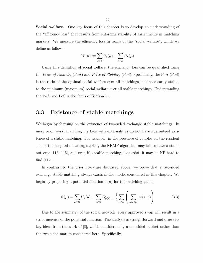
54

Social welfare. One key focus of this chapter is to develop an understanding of

the “efficiency loss” that results from enforcing stability of assignments in matching

markets. We measure the efficiency loss in terms of the “social welfare”, which we

define as follows:

W (µ) :=�

s∈S

Us(µ) +�

h∈H

Uh(µ)

Using this definition of social welfare, the efficiency loss can be quantified using

the Price of Anarchy (PoA) and Price of Stability (PoS). Specifically, the PoA (PoS)

is the ratio of the optimal social welfare over all matchings, not necessarily stable,

to the minimum (maximum) social welfare over all stable matchings. Understanding

the PoA and PoS is the focus of Section 3.5.

3.3 Existence of stable matchings

We begin by focusing on the existence of two-sided exchange stable matchings. In

most prior work, matching markets with externalities do not have guaranteed exis-

tence of a stable matching. For example, in the presence of couples on the resident

side of the hospital matching market, the NRMP algorithm may fail to have a stable

outcome [113, 115], and even if a stable matching does exist, it may be NP-hard to

find [112].

In contrast to the prior literature discussed above, we prove that a two-sided

exchange stable matching always exists in the model considered in this chapter. We

begin by proposing a potential function Φ(µ) for the matching game:

Φ(µ) =�

h∈H

Uh(µ) +�

s∈S

Ds

µ(s) +1

2

�

s∈S

�

x∈µ2(s)

w(s, x)

(3.3)

Due to the symmetry of the social network, every approved swap will result in a

strict increase of the potential function. The analysis is straightforward and draws its

key ideas from the work of [8], which considers only a one-sided market rather than

the two-sided market considered here. Specifically,

55

Lemma 3.1. Any swap matching µt

sfor which (i) and (ii) below are satisfied, Φ(µt

s) >

Φ(µ).

(i) ∀ i ∈ {s, t, µ(s), µ(t)}, Ui(µt

s) ≥ Ui(µ), and

(ii) ∃ i ∈ {s, t, µ(s), µ(t)} with Ui(µt

s) > Ui(µ)

Proof. We begin by calculating the difference in the potential function for a swap

matching using (3.3), assuming that µ(s) = h and µ(t) = g:4

Φ(µt

s)− Φ(µ) =

�

h∈H

Uh(µt

s)− Uh(µ) +

�

s∈S

Ds

µts(s)

−Ds

µ(s)

+1

2

�

s∈S

�

x∈µts(s)

w(s, x)

− 1

2

�

s∈S

�

x∈µ(s)

w(s, x)

(3.4)

Expanding and canceling like terms, we have

Φ(µt

s)− Φ(µ) = Uh(µ

t

s)− Uh(µ) + Ug(µ

t

s)− Ug(µ) +Ds

g−Dt

g+Dt

h−Ds

h

+1

2

�

x∈µ(g)

w(s, x)− w(s, t) +�

x∈µ(h)

w(t, x)− w(s, t)

+

�

x∈µ(g)

w(x, s)− w(s, t) +�

x∈µ(h)

w(x, t)− w(s, t)

− 1

2

�

x∈µ(h)

w(s, x) +�

x∈µ(g)

w(t, x)

+

�

x∈µ(h)

w(x, s) +�

x∈µ(g)

w(x, t)

(3.5)

4Note that we have a little abuse of notation here, for convenience. We are using x ∈ µts(s)

to denote the the other students x that are in the same house as s under the swap matching µts.

Similarly, x ∈ µ(s) denotes the other students that are in the same house as s under the originalmatching µ. We revert to the correct notation in (3.5).

56

which becomes, due to the symmetry of the social network,

Φ(µt

s)− Φ(µ) = Uh(µ

t

s)− Uh(µ) + Ug(µ

t

s)− Ug(µ) +Ds

g−Dt

g+Dt

h−Ds

h

+�

x∈µ(g)

(w(s, x)− w(t, x)) +�

x∈µ(h)

(w(t, x)− w(s, x))− 2w(s, t)

(3.6)

Note that if t is a “hole”, this becomes

Φ(µt

s)− Φ(µ) = Uh(µ

t

s)− Uh(µ) + Ug(µ

t

s)− Ug(µ) +Ds

g−Ds

h

+�

x∈µ(g)

(w(s, x))−�

x∈µ(h)

(w(s, x)) (3.7)

Now, consider a matching µ and a swap matching µt

sthat satisfies (i) and (ii)

from the lemma statement. Without loss of generality, assume that student s strictly

improves. The other student could be either a “hole” or a real student that either

improves or is indifferent to the swap. The other cases are symmetric. Define µ(s) =

h, and µ(t) = g. The change in utility for student s is then

0 < Us(µt

s)− Us(µ) = Ds

g−Ds

h−

�

x∈µ(h)

w(s, x) +�

x∈µ(g)

w(s, x)− w(s, t),

Similarly, for student t, we have

0 ≤ Ut(µt

s)− Ut(µ) = Dt

h−Dt

g−

�

x∈µ(g)

w(t, x) +�

x∈µ(h)

w(t, x)− w(s, t).

Adding the above inequalities, we obtain the following:

0 < Ds

g−Dt

g+Dt

h−Ds

h+

�

x∈µ(g)

(w(s, x)− w(t, x))+�

x∈µ(h)

(w(t, x)− w(s, x))−2w(s, t) := δs,t

Note that we are using δs,t to denote the change in utilities for the two students, s

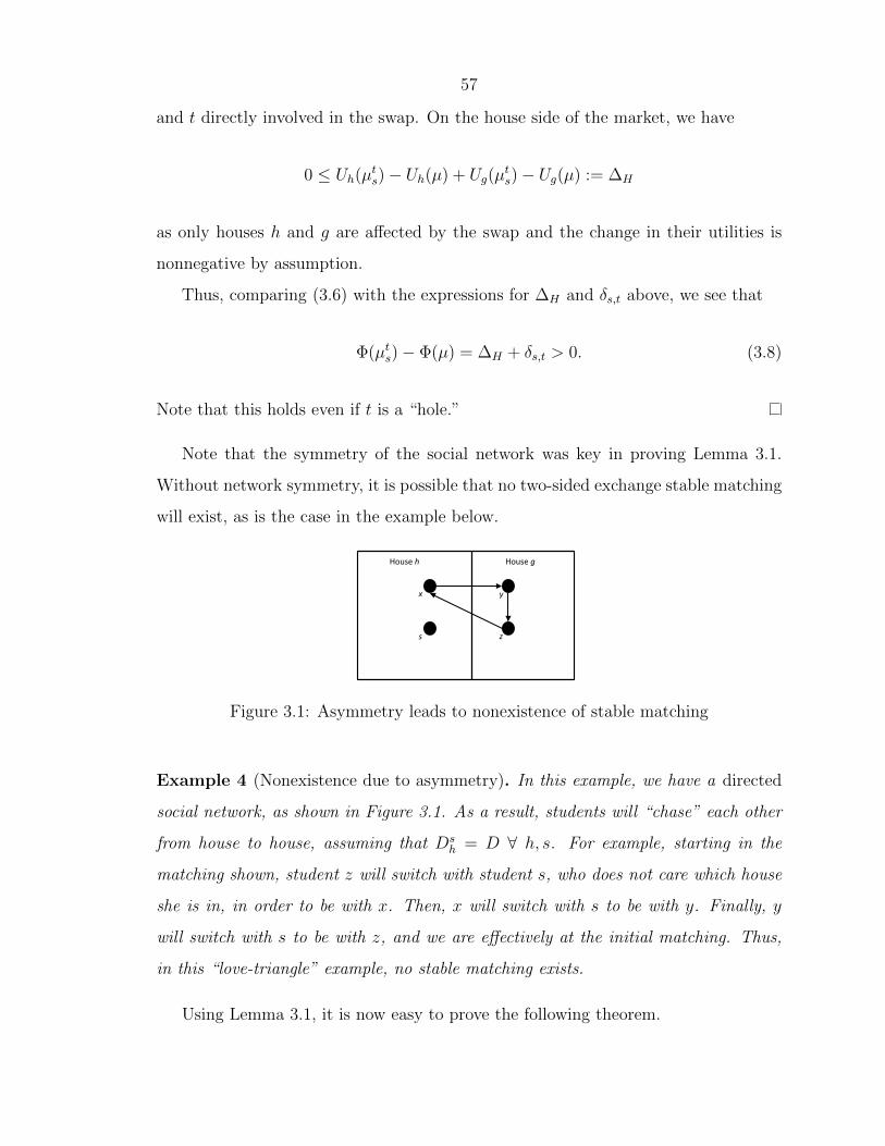
57

and t directly involved in the swap. On the house side of the market, we have

0 ≤ Uh(µt

s)− Uh(µ) + Ug(µ

t

s)− Ug(µ) := ∆H

as only houses h and g are affected by the swap and the change in their utilities is

nonnegative by assumption.

Thus, comparing (3.6) with the expressions for ∆H and δs,t above, we see that

Φ(µt

s)− Φ(µ) = ∆H + δs,t > 0. (3.8)

Note that this holds even if t is a “hole.”

Note that the symmetry of the social network was key in proving Lemma 3.1.

Without network symmetry, it is possible that no two-sided exchange stable matching

will exist, as is the case in the example below.

!"#$%&!& !"#$%&"&

#$ %$

&$'$

Figure 3.1: Asymmetry leads to nonexistence of stable matching

Example 4 (Nonexistence due to asymmetry). In this example, we have a directed

social network, as shown in Figure 3.1. As a result, students will “chase” each other

from house to house, assuming that Ds

h= D ∀ h, s. For example, starting in the

matching shown, student z will switch with student s, who does not care which house

she is in, in order to be with x. Then, x will switch with s to be with y. Finally, y

will switch with s to be with z, and we are effectively at the initial matching. Thus,

in this “love-triangle” example, no stable matching exists.

Using Lemma 3.1, it is now easy to prove the following theorem.

58

Theorem 3.2. All local maxima of Φ(µ) are two-sided exchange stable.

Proof. Let matching µ be a local maximum of Φ(µ). Assume, by way of contradiction,

that µ is not two-sided exchange stable. Lemma 3.1 shows that any swap matching

that is acceptable to all parties (i.e., satisfies conditions (i) and (ii)) strictly increases

Φ(µ). But this contradicts the assumption that µ is a local maximum. Thus, µ must

be two-sided exchange stable.

As the number of matches is finite, the global maximum of the potential func-

tion must be two-sided exchange stable, and, therefore, a two-sided exchange stable

matching will always exist for every housing assignment market of this form.

3.3.1 Special case: Objective desirability

If we assume that there are no vacancies in any of the houses and students value

houses according to the same rules (i.e., Ds

h= Dt

h∀ s �= t), then each each approved

swap will result in a strict increase in the social welfare. Specifically,

Lemma 3.3. If house quotas are exactly met and Ds

h= Dt

h∀ s �= t, then any swap

matching µt

sfor which

(i) ∀ i ∈ {s, t, µ(s), µ(t)}, Ui(µt

s) ≥ Ui(µ), and

(ii) ∃ i ∈ {s, t, µ(s), µ(t)} with Ui(µt

s) > Ui(µ)

has W (µt

s) > W (µ).

Proof. Consider a matching µ and a swap matching µt

sthat satisfies (i) and (ii)

from the lemma statement. Note that due to the assumption that the house quotas

are all met, the swap must be between two students, not a student and a “hole”.

Without loss of generality, assume that student s strictly improves. The other cases

are symmetric. Define µ(s) = h, and µ(t) = g. The change in utility for student s is

then

0 < Us(µt

s)− Us(µ) = Dg −Dh −

�

x∈µ(h)

w(s, x) +�

x∈µ(g)

w(s, x)− w(s, t),

59

Similarly, for student t, we have

0 ≤ Ut(µt

s)− Ut(µ) = Dh −Dg −

�

x∈µ(g)

w(t, x) +�

x∈µ(h)

w(t, x)− w(s, t).

Adding the above inequalities, we obtain the following:

0 <�

x∈µ(g)

(w(s, x)− w(t, x)) +�

x∈µ(h)

(w(t, x)− w(s, x))− 2w(s, t) := δs,t

Continuing, the total change in utility for all students is:

∆S :=�

x∈S

Ux(µt

s)−

�

x∈S

Ux(µ)

= δs,t +�

x∈µ(g)

w(x, s)− w(s, t)

� �� �gain from s joining g

−�

x∈µ(h)

w(x, s)

� �� �loss from s leaving h

+�

x∈µ(h)

w(x, t)− w(s, t)

� �� �gain from t joining h

−�

x∈µ(g)

w(x, t)

� �� �loss from t leaving g

= 2δs,t (3.9)

> 0

where line (3.9) comes from the fact that we assume the social network graph is

symmetric.

On the house side of the market, we have

0 ≤ Uh(µt

s)− Uh(µ) + Ug(µ

t

s)− Ug(µ) := ∆H

as only houses h and g are affected by the swap and the change in their utilities is

nonnegative by assumption. Thus, the total social welfare strictly increases:

W (µt

s)−W (µ) = ∆S +∆H > 0

As before, it is now easy to prove the following theorem.

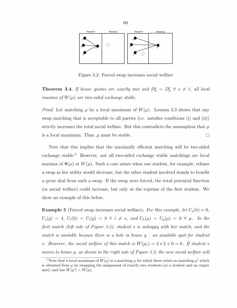
60

!"

#"

$"

%"

#"

$"

%"!"

&'(!)"!" &'(!)"!" &'(!)"""&'(!)"""

Figure 3.2: Forced swap increases social welfare

Theorem 3.4. If house quotas are exactly met and Ds

h= Dt

h∀ s �= t, all local

maxima of W (µ) are two-sided exchange stable.

Proof. Let matching µ be a local maximum of W (µ). Lemma 3.3 shows that any

swap matching that is acceptable to all parties (i.e. satisfies conditions (i) and (ii))

strictly increases the total social welfare. But this contradicts the assumption that µ

is a local maximum. Thus, µ must be stable.

Note that this implies that the maximally efficient matching will be two-sided

exchange stable.5 However, not all two-sided exchange stable matchings are local

maxima of Φ(µ) or W (µ). Such a case arises when one student, for example, refuses

a swap as her utility would decrease, but the other student involved stands to benefit

a great deal from such a swap. If the swap were forced, the total potential function

(or social welfare) could increase, but only at the expense of the first student. We

show an example of this below.

Example 5 (Forced swap increases social welfare). For this example, let Us(h) = 0,

Us(g) = 4, Ui(h) = Ui(g) = 0 ∀ i �= s, and Uh(µ) = Ug(µ) = 0 ∀ µ. In the

first match (left side of Figure 3.2), student s is unhappy with her match, and the

match is unstable because there is a hole in house g – an available spot for student

s. However, the social welfare of this match is W (µ1) = 2 ∗ 3 + 0 = 6. If student s

moves to house g, as shown in the right side of Figure 3.2, the new social welfare will

5Note that a local maximum of W (µ) is a matching µ for which there exists no matching µ� whichis obtained from µ by swapping the assignment of exactly two students (or a student and an emptyspot) and has W (µ�) > W (µ).

61

be W (µ2) = 0 + 4 = 4. Note that this matching is stable, since s does not want to

move from house g. If we force the s back to h, we can increase the social welfare.

The contrast between Theorem 3.2 and results such as [113] and [115] can be ex-

plained by considering a few aspects of the model we study. In particular, we are using

a distinct type of stability appropriate to our housing assignment market. Further,

the assumption that the social network graph is symmetric is key to guaranteeing

existence.

3.4 Finding stable matchings

In the previous section we have shown that a two-sided exchange stable matching

will always exist and, moreover, that under certain assumptions, socially optimal

matchings are two-sided exchange stable. In this section, we turn to the task of

developing algorithms for finding two-sided exchange stable matchings. In particular,

two natural algorithms follow immediately from our analysis. For simplicity, in this

section we assume the conditions of Theorem 3.4; namely, that quotas are exactly

met and students rate houses according to the same rules.6

Algorithm 1 (Greedy)

while i ≤ maxIterations doSearch for “approved” swap µt

s

µ ← µt

s

i ← i+ 1end while

Algorithm 1 proceeds by greedily considering “approved” swaps among students/houses

that improve the social welfare. Note that this algorithm can easily be implemented

in a distributed manner, and loosely models the process by which individuals adjust

a matching that is not stable. For example, consider starting at a random matching,

and giving students a preset amount of time to talk amongst themselves and make

6We note that the results of this section extend to the more general case, using the potentialfunction defined in Section 3.3 rather than the social welfare function.

62

swaps, obtaining the approval of their houses for each swap. Given enough time, such

a distributed method will converge to a 2ES match.

Lemma 3.3 and Theorem 3.4 immediately give that Algorithm 1 will converge to

a two-sided exchange stable matching, since the social welfare strictly improves with

each iteration, and all local maxima of W are two-sided exchange stable matchings.

Note that Algorithm 1 is not guaranteed to converge to the socially optimal stable

matching; it will likely find just a local maxima of W . Also, note that each iteration

of the algorithm above can involve searching many pairs of students (and houses) for

an “approved” swap.

Algorithm 2 MCMC

while i ≤ maxIterations doPick random pair of students {s, t}PT = 1

1+e−T (W (µts)−W (µ))

µ ← µt

swith probability PT

if (W (µt

s) > Wbest) then

Wbest = W (µt

s)

end ifi ← i+ 1

end while

The second algorithm we consider again seeks to optimize W , this time using a

MCMC heat bath. In this algorithm we start with a random initial matching and

at each iteration swap a random pair of students with a probability that depends on

the change in social welfare: a positive change yields a probability of swapping larger

than 1/2 and vice versa. Algorithm 2 therefore can emerge from a local maximum.

The algorithm keeps track of the “best” matching found so far, even as it moves to

worse matchings. If Algorithm 2 is run sufficiently long (perhaps exponential time)

it can find the optimal two-sided exchange stable matching [59]. However, there is

no guarantee that the best matching encountered in finite time is even two-sided

exchange stable, a situation that can be remedied by applying the greedy algorithm

to this matching. Simulation results show the superiority of Algorithm 2 to Algorithm

1 in terms of welfare, at the expense of an increase in the number of computations.

To illustrate the performance of these two algorithms, we use two social network data

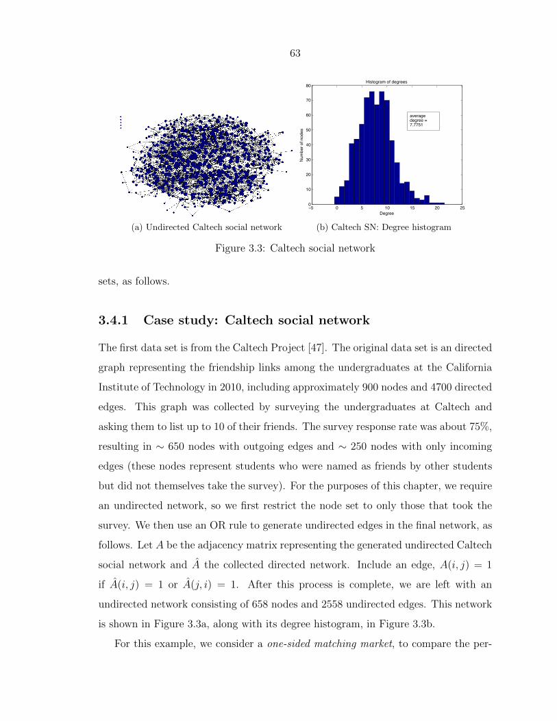
63

(a) Undirected Caltech social network

−5 0 5 10 15 20 250

10

20

30

40

50

60

70

80Histogram of degrees

Degree

Num

ber o

f nod

es

averagedegree =7.7751

(b) Caltech SN: Degree histogram

Figure 3.3: Caltech social network

sets, as follows.

3.4.1 Case study: Caltech social network

The first data set is from the Caltech Project [47]. The original data set is an directed

graph representing the friendship links among the undergraduates at the California

Institute of Technology in 2010, including approximately 900 nodes and 4700 directed

edges. This graph was collected by surveying the undergraduates at Caltech and

asking them to list up to 10 of their friends. The survey response rate was about 75%,

resulting in ∼ 650 nodes with outgoing edges and ∼ 250 nodes with only incoming

edges (these nodes represent students who were named as friends by other students

but did not themselves take the survey). For the purposes of this chapter, we require

an undirected network, so we first restrict the node set to only those that took the

survey. We then use an OR rule to generate undirected edges in the final network, as

follows. Let A be the adjacency matrix representing the generated undirected Caltech

social network and A the collected directed network. Include an edge, A(i, j) = 1

if A(i, j) = 1 or A(j, i) = 1. After this process is complete, we are left with an

undirected network consisting of 658 nodes and 2558 undirected edges. This network

is shown in Figure 3.3a, along with its degree histogram, in Figure 3.3b.

For this example, we consider a one-sided matching market, to compare the per-

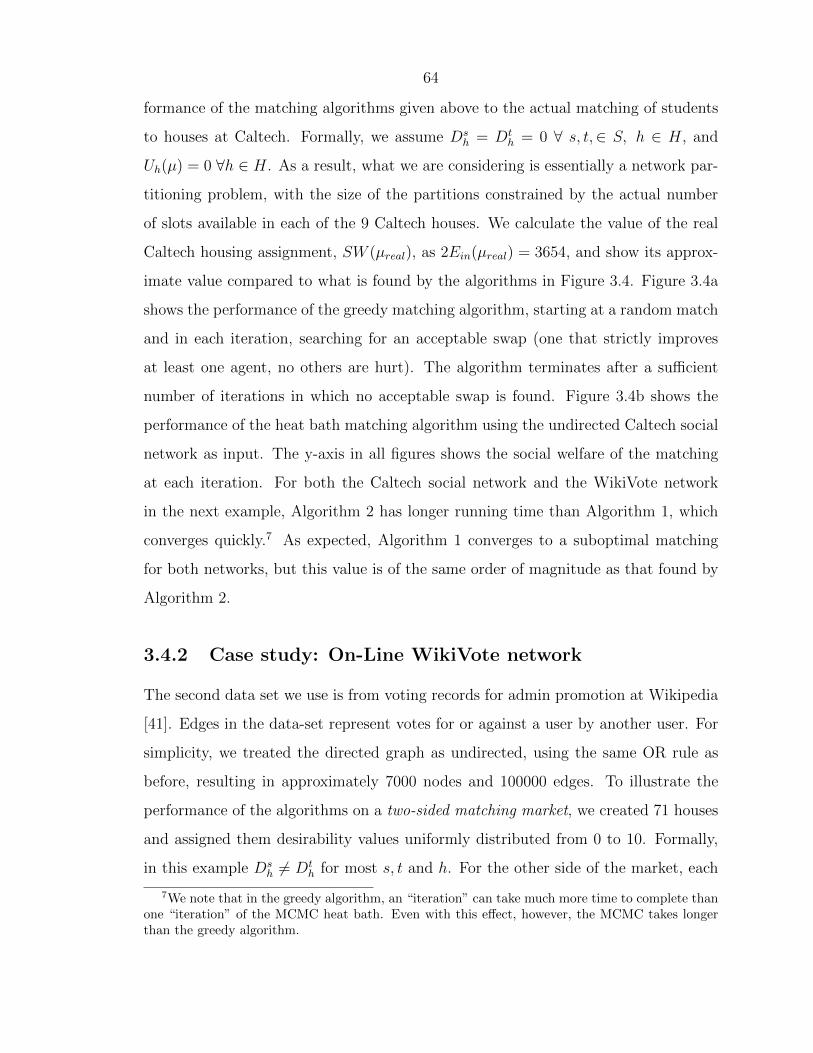
64

formance of the matching algorithms given above to the actual matching of students

to houses at Caltech. Formally, we assume Ds

h= Dt

h= 0 ∀ s, t,∈ S, h ∈ H, and

Uh(µ) = 0 ∀h ∈ H. As a result, what we are considering is essentially a network par-

titioning problem, with the size of the partitions constrained by the actual number

of slots available in each of the 9 Caltech houses. We calculate the value of the real

Caltech housing assignment, SW (µreal), as 2Ein(µreal) = 3654, and show its approx-

imate value compared to what is found by the algorithms in Figure 3.4. Figure 3.4a

shows the performance of the greedy matching algorithm, starting at a random match

and in each iteration, searching for an acceptable swap (one that strictly improves

at least one agent, no others are hurt). The algorithm terminates after a sufficient

number of iterations in which no acceptable swap is found. Figure 3.4b shows the

performance of the heat bath matching algorithm using the undirected Caltech social

network as input. The y-axis in all figures shows the social welfare of the matching

at each iteration. For both the Caltech social network and the WikiVote network

in the next example, Algorithm 2 has longer running time than Algorithm 1, which

converges quickly.7 As expected, Algorithm 1 converges to a suboptimal matching

for both networks, but this value is of the same order of magnitude as that found by

Algorithm 2.

3.4.2 Case study: On-Line WikiVote network

The second data set we use is from voting records for admin promotion at Wikipedia

[41]. Edges in the data-set represent votes for or against a user by another user. For

simplicity, we treated the directed graph as undirected, using the same OR rule as

before, resulting in approximately 7000 nodes and 100000 edges. To illustrate the

performance of the algorithms on a two-sided matching market, we created 71 houses

and assigned them desirability values uniformly distributed from 0 to 10. Formally,

in this example Ds

h�= Dt

hfor most s, t and h. For the other side of the market, each

7We note that in the greedy algorithm, an “iteration” can take much more time to complete thanone “iteration” of the MCMC heat bath. Even with this effect, however, the MCMC takes longerthan the greedy algorithm.

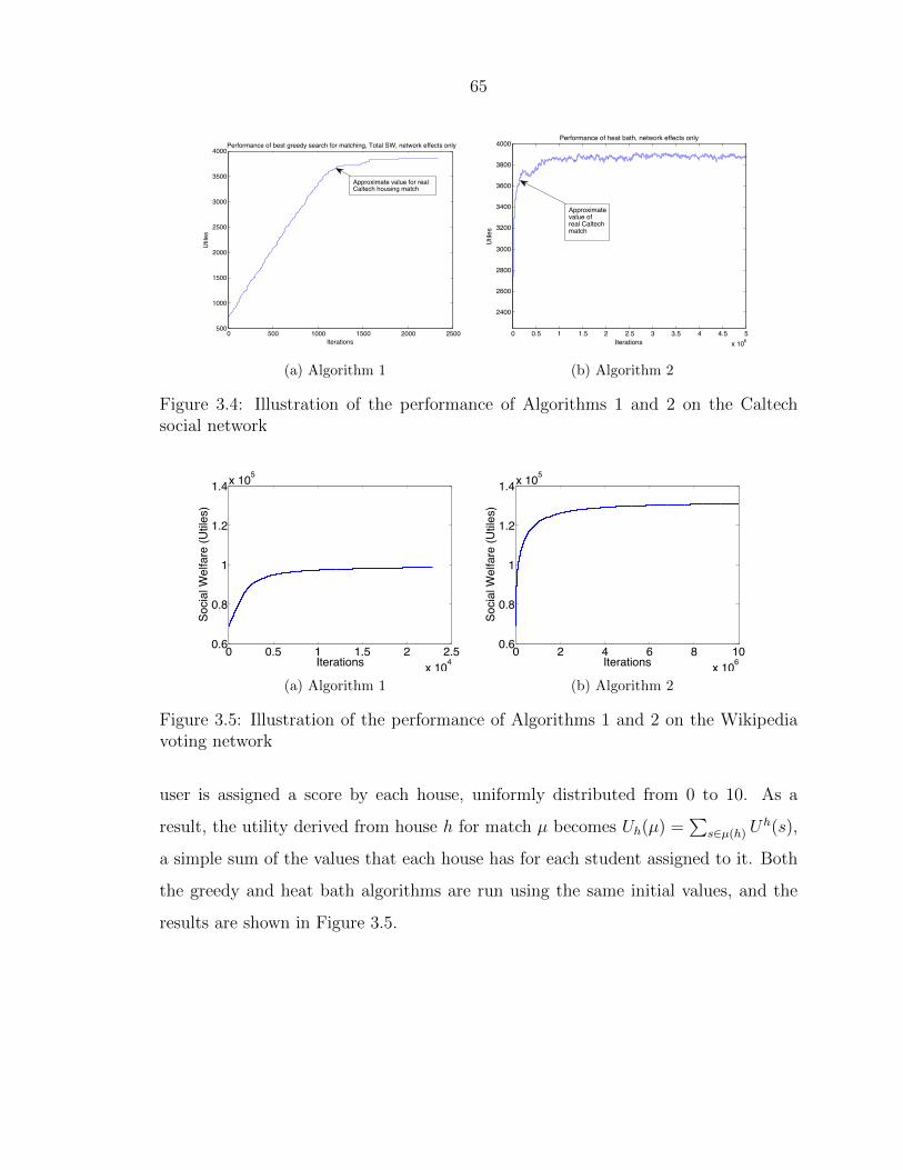
65

0 500 1000 1500 2000 2500500

1000

1500

2000

2500

3000

3500

4000

Iterations

Util

es

Performance of best greedy search for matching, Total SW, network effects only

Approximate value for realCaltech housing match

(a) Algorithm 1

0 0.5 1 1.5 2 2.5 3 3.5 4 4.5 5x 106

2400

2600

2800

3000

3200

3400

3600

3800

4000

Iterations

Util

es

Performance of heat bath, network effects only

Approximatevalue ofreal Caltechmatch

(b) Algorithm 2

Figure 3.4: Illustration of the performance of Algorithms 1 and 2 on the Caltechsocial network

0 0.5 1 1.5 2 2.5x 104

0.6

0.8

1

1.2

1.4x 105

Iterations

Soci

al W

elfa

re (U

tiles

)

(a) Algorithm 1

0 2 4 6 8 10x 106

0.6

0.8

1

1.2

1.4x 105

Iterations

Soci

al W

elfa

re (U

tiles

)

(b) Algorithm 2

Figure 3.5: Illustration of the performance of Algorithms 1 and 2 on the Wikipediavoting network

user is assigned a score by each house, uniformly distributed from 0 to 10. As a

result, the utility derived from house h for match µ becomes Uh(µ) =�

s∈µ(h) Uh(s),

a simple sum of the values that each house has for each student assigned to it. Both

the greedy and heat bath algorithms are run using the same initial values, and the

results are shown in Figure 3.5.

66

3.5 Efficiency of stable matchings

To this point, we have focused on the existence of two-sided exchange stable matchings

and how to find them. In this section our focus is on the “efficiency loss” due to

stability in a matching market and the role peer effects play in this efficiency loss.

We measure the efficiency loss in a matching market using the price of stability

(PoS) and the price of anarchy (PoA) as defined in Section 3.2. Interestingly, the

price of anarchy has multiple interpretations in the context of this chapter. First,

as is standard, it measures the worst-case loss of social welfare that results due to

enforcing exchange stability. For example, the authors in [6] bound the loss in social

welfare caused by individual rationality (by enforcing stable matchings) for matching

markets without externalities. Second, it provides a competitive ratio for Algorithm

1 for finding a stable matching, since Algorithm 1 provides no guarantee about which

stable matching it will find. Third, we show later that the price of anarchy also has

an interpretation as capturing the efficiency lost due to peer effects.

The results in this section all require one additional simplifying assumption to our

model: complementarities are ignored and only peer effects are considered. Specifi-

cally, we assume, for all of our PoA results, Uh(µ) = 0, and thus W (µ) =�

s∈S Us(µ).

Under this assumption, the market is one-sided, with only students participating —

as a result we are only considering exchange stability. This assumption is limiting, but

there are still many settings within which the model is appropriate. Two examples

are the housing assignment problem in the case when students can swap positions

without needing house approval, and the assignment of faculty to offices as discussed

in [8], as clearly the offices have no preferences over which faculty occupy them. In

order to simplify the analysis, we also make use of the assumptions in Theorem 3.4:

(i) Ds

h= Dt

h∀ s �= t and (ii) house quotas are exactly met.

3.5.1 Related models

When the housing assignment problem is restricted to a one-sided market involving

only students, we note that it becomes very similar to both (i) a hedonic coalition

67

formation game with symmetric additively separable preferences, as described in [21],

and (ii) a coalitional affinity game, as described in [28].

In hedonic coalition formation games, agents’ preferences for a given coalition are

based on the other members of that coalition [42]. Note that coalition games are nec-

essarily one-sided — agents care about the coalitions but the coalitions cannot care

about the agents. The most related work to ours in this area is [21], where the au-

thors show that when agents’ preferences over coalition are symmetric and additively

separable (as the student utility functions in the housing assignment problem are),

a Nash (and individually) stable coalition structure will always exist. This mimics

the existence result proved in Section 3.3, however our result applies for a two-sided

market. Further work on hedonic games looks at the complexity of finding stable

coalition structures; see [7, 29, 46, 53, 95] for examples.

Coalitional affinity games consider the pairwise relationships between agents, as

represented by a weighted graph [28], and are a special subclass of hedonic games.

The most related result to the current work is [28], which proves a tight upper bound

on the Price of Anarchy using the notion of core stability8 when the weighted graph

is symmetric.

While the one-sided housing assignment problem and hedonic coalition formation

games appear to be very similar, there are a number of key differences. Most im-

portantly, the housing assignment problem considers a fixed number of houses with

a limited number of spots available; students cannot break away and form a new

coalition/house, nor can a house have more students than its quota. In addition, our

model considers exchange stability, which is closest to the Nash stability of [21], but

is still significantly different in that it involves a pair of students willing and able

to swap. Finally, each student gains utility from the house they are matched with,

in addition to the other members of that house, which is different from the original

formulation of hedonic coalition games.

8A coalition structure is core stable if no set of agents can break away and form a new coalitionto improve their own utility.

68

k

1 1Dh = 0

Dg = 0

Dh = 0 Dg = 0k

1 1

(a) optimal matching (b) stable matching

Figure 3.6: Arbitrarily bad exchange stable matching

3.5.2 Discussion of results

To begin the discussion of our results, note that, as discussed in Section 3.3, the

price of stability is 1 for our model because any social welfare optimizing matching is

stable.

However, the price of anarchy can be much larger than 1. In fact, depending on

the social network, the price of anarchy can be unboundedly large, as illustrated in

the following example.

Example 6 (Unbounded price of anarchy). Consider a matching market with 4 stu-

dents and 2 houses, each with a quota of 2, and two possible matchings illustrated by

Figure 3.6. As shown in Figure 3.6 (a) and (b), respectively, in the optimal matching

µ∗, W (µ∗) = k; whereas there exists a exchange stable matching with W (µ) = 2.

Thus, as k increases, the price of anarchy grows linearly in k.

Despite the fact that, in general, there is a large efficiency loss that results from

enforcing exchange stability, in many realistic cases the efficiency loss is actually quite

small. The following two theorems provide insight into such cases.

A key parameter in these theorems is γ∗m

which captures how well the social

network can be “clustered” into a fixed number of m groups and is defined as follows.

γm(µ) :=Ein(µ)

|E| (3.10)

γ∗m:= max

µ

γm(µ) (3.11)

Thus, γ∗mrepresents the maximum edges that can be captured by a partition satisfying

the house quotas. Note that γ∗mis highly related to other clustering metrics, such as

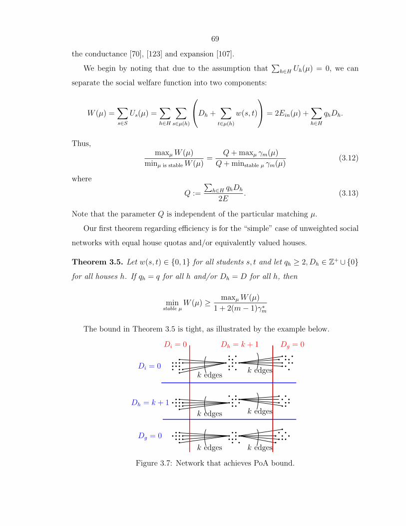
69

the conductance [70], [123] and expansion [107].

We begin by noting that due to the assumption that�

h∈H Uh(µ) = 0, we can

separate the social welfare function into two components:

W (µ) =�

s∈S

Us(µ) =�

h∈H

�

s∈µ(h)

Dh +�

t∈µ(h)

w(s, t)

= 2Ein(µ) +�

h∈H

qhDh.

Thus,maxµ W (µ)

minµ is stable W (µ)=

Q+maxµ γm(µ)

Q+minstable µ γm(µ)(3.12)

where

Q :=

�h∈H qhDh

2E. (3.13)

Note that the parameter Q is independent of the particular matching µ.

Our first theorem regarding efficiency is for the “simple” case of unweighted social

networks with equal house quotas and/or equivalently valued houses.

Theorem 3.5. Let w(s, t) ∈ {0, 1} for all students s, t and let qh ≥ 2, Dh ∈ Z+ ∪ {0}for all houses h. If qh = q for all h and/or Dh = D for all h, then

minstable µ

W (µ) ≥ maxµ W (µ)

1 + 2(m− 1)γ∗m

The bound in Theorem 3.5 is tight, as illustrated by the example below.

k edges

Di = 0 Dg = 0Dh = k + 1

Di = 0

Dg = 0

Dh = k + 1

k edges

k edges

k edges

k edges

k edges

Figure 3.7: Network that achieves PoA bound.

70

Example 7 (Tightness of Theorem 3.5). Consider a setting with m houses and qh =

mk for all h ∈ H. Students are grouped into clusters of size k > 2, as shown for

m = 3 in Figure 3.7. The houses have Dh = k + 1 and Dg = Di = 0. Each student

in the middle cluster in each row has k edges to the other students outside of their

cluster (but none within), as shown.

The worst-case stable exchange-matching is represented by the vertical red lines.

Note that since Dh = k + 1, this matching is stable, even though all edges are cut.

Thus minµ stable γm(µ) = 0. The optimal matching is represented by the horizontal

blue lines in the figure; note that γ∗m= 1. To calculate the price of anarchy, we start

from equations (3.12) and (3.13) and calculate

Q =

�h∈H qhDh

2|E| =mk(k + 1)

2mk(m− 1)k=

k + 1

2(m− 1)k,

which gives,

maxµ W (µ)

minstable µ W (µ)=

Q+ γ∗m

Q+minµ stable γm(µ)= 1 + 2(m− 1)

�k

k + 1

�.

Notice that as k becomes large, this approaches the bound of 1 + 2(m− 1)γ∗m.

We note that the requirement qh = q for all h and/or Dh = D for all h is key to

the proof of Theorem 3.5 and in obtaining such a simple bound; otherwise, Theorem

3.6 applies. We omit the proofs of these theorems here for brevity; see Section 3.7 for

the details.

Our second theorem removes the restrictions in the theorem above, at the expense

of a slightly weaker bound. Define qmax = maxh∈H qh, wmax = maxs,t∈S w(s, t) and

D∆ = minh,g∈H(Dh −Dg), assuming that the houses are ordered in increasing values

of Dh.

Theorem 3.6. Let w(s, t) ∈ R+∪{0} for all students s, t and Dh ∈ R+∪{0}, qh ∈ Z+

for all houses h, then

minstable µ

W (µ) ≥ maxµ W (µ)

1 + 2(m− 1)�γ∗m+ qmaxwmax

D∆

�

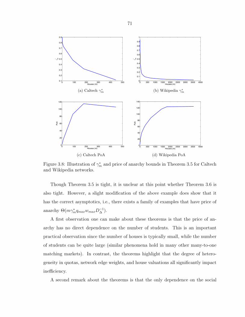
71

0 100 200 300 400 5000.1

0.2

0.3

0.4

0.5

0.6

0.7

0.8

0.9

Houses (m)

m*

(a) Caltech γ∗m

0 500 1000 1500 2000 2500 3000 3500 40000

0.1

0.2

0.3

0.4

0.5

0.6

0.7

0.8

0.9

1

Houses (m)

m*

(b) Wikipedia γ∗m

0 100 200 300 400 5000

20

40

60

80

100

120

Houses (m)

PoA

(c) Caltech PoA

0 500 1000 1500 2000 2500 3000 3500 40000

20

40

60

80

100

120

140

Houses (m)

PoA

(d) Wikipedia PoA

Figure 3.8: Illustration of γ∗mand price of anarchy bounds in Theorem 3.5 for Caltech

and Wikipedia networks.

Though Theorem 3.5 is tight, it is unclear at this point whether Theorem 3.6 is

also tight. However, a slight modification of the above example does show that it

has the correct asymptotics, i.e., there exists a family of examples that have price of

anarchy Θ(mγ∗mqmaxwmaxD

−1∆ ).

A first observation one can make about these theorems is that the price of an-

archy has no direct dependence on the number of students. This is an important

practical observation since the number of houses is typically small, while the number

of students can be quite large (similar phenomena hold in many other many-to-one

matching markets). In contrast, the theorems highlight that the degree of hetero-

geneity in quotas, network edge weights, and house valuations all significantly impact

inefficiency.

A second remark about the theorems is that the only dependence on the social

72

network is through γ∗m, which measures how well the graph can be “clustered” into m

groups. An important note about γ∗m

is that it is highly dependent on m, and tends

to shrink quickly as m grows. We give an illustration of this effect in Figures 3.8a and

3.8b using the two social network data sets described in Section 3.4. A consequence

of this behavior is that the price of anarchy is not actually linear in m in Theorems

3.5 and 3.6, as it may first appear, it turns out to be sublinear. This is illustrated in

the context of real social network data in Figures 3.8c and 3.8d. We note that as we

are increasing m, what we are in fact doing is creating finer allowable partitions of

the network.

Next, let us consider the impact of peer effects on the price of anarchy. Considering

the simple setting of Theorem 3.5, we see that if there were no peer effects, this would

be equivalent to setting w(s, t) = 0 for all s, t. This would imply that γ∗m= 0, and so

the price of anarchy is one. Thus, another interpretation of the price of anarchy in

Theorem 3.5 is the efficiency lost as a result of peer effects.

3.6 Concluding remarks

In this chapter we have focused on many-to-one matchings with peer effects and com-

plementarities. Typically, results on this topic tend to be negative, either proving that

stable matchings may not exist, e.g., [113, 115], or that stable matchings are compu-

tationally difficult to find, e.g., [112]. Our goal has been to provide positive results.

To this end, we focus on the case when peer effects are the result of an underlying

social network, and this restriction on the form of the peer effects allows us to prove

that a two-sided exchange-stable matching always exists and that socially optimal

matchings are always stable. Further, we provide bounds on the maximal inefficiency

(price of anarchy) of any exchange-stable matching and show how this inefficiency

depends on the clustering properties of the social network graph. Interestingly, in our

context the price of anarchy has a dual interpretation as characterizing the degree of

inefficiency caused by peer effects.

There are numerous examples of many-to-one matchings where the results in this

73

chapter can provide insight; one of particular interest to us is the matching of incom-

ing undergraduates to residential houses which happens yearly at Caltech and other

universities. Currently incoming students only report a preference order for houses,

and so are incentivized to collude with friends and not reveal their true preferences.

For such settings, the results in this chapter highlight the importance of having stu-

dents report not only their preference order on houses, but also a list of friends with

whom they would like to be matched. In particular, our simulations in Section 3.4

clearly show an improvement in social welfare by considering the social network in

the matching mechanism. Using a combination of these factors the algorithms and

efficiency bounds presented in this chapter provide a promising approach, for this

specific market as well as any general market where peer effects change the space of

stable matchings.

Our current results represent only a starting point for research into the interaction

of social networks and many-to-one matchings. There are a number of simplifying

assumptions in this work which would be interesting to relax. For example, the

efficiency bounds we have proven consider only a one-sided market, where houses

do not have preferences over students, students rate houses similarly, and quotas

are exactly met. These assumptions are key to providing simpler bounds, and they

certainly are valid in some matching markets; however relaxing these assumptions

would broaden the applicability of the work greatly.

3.7 Appendix: Proofs of Theorems 3.5 and 3.6

We note that these proofs hold for the one-sided market; i.e., when Uh(µ) = 0 ∀h ∈ H,

where the quotas for the houses are exactly satisfied; i.e., there are no “holes”, and

students value houses according to the same rules; i.e., Ds

h= Dt

h∀ s �= t, h ∈ H.

Also note that for ease of notation, we use E instead of |E| to represent the total

edge weight of the graph in this section.

74

3.7.1 Proof of Theorem 3.5

Throughout the proof we assume that the houses are ordered: i.e., if g < h then

Dg < Dh. An important tool that we use throughout the proof is a rephrasing of the

definition of exchange stability in the one-sided market case in terms of a function α

as follows.

Definition 5. Let αµ(s, g) be a function representing the benefit a student s gains by

moving to house g under matching µ:

αµ(s, g) = Dg −Dµ(s) +�

x∈µ(g)

w(s, x)−�

x∈µ2(s)

w(s, x) (3.14)

Notice that using the definition above, given a specific swap matching µt

swhere

t ∈ µ(g), we can calculate the difference in utility for the involved student s as

Us(µt

s)− Us(µ) = αµ(s, g)− w(s, t)

because�

x∈µts(g)

w(s, x) =�

x∈µ(g) w(s, x)− w(s, t).

The definition of α also provides a useful new phrasing of the definition of exchange

stability, which is equivalent to that of Definition 4 when the market is one-sided, i.e,

when Uh(µ) = 0 ∀h ∈ H. Note that we are only considering the Price of Anarchy for

the one-sided market here – we plan to generalize these results for the two-sided case

in future work.

Definition 6. A matching µ is exchange stable (ES) in the one-sided (students-

only) housing assignment market if and only if for all pairs of students s ∈ µ(h) and

t ∈ µ(g), at least one of the following conditions holds:

(Condition 1) s doesn’t want to swap, i.e., αµ(s, g) < w(s, t).

(Condition 2) t doesn’t want to swap, i.e., αµ(t, h) < w(s, t).

(Condition 3) s and t are indifferent, i.e., αµ(s, g) = αµ(t, h) = w(s, t).

75

Using the above rephrasing of the definition of exchange stability, we now continue

with the proof of Theorem 3.5. In order to prove an upper bound on the price of

anarchy, we prove a lower bound on γm(µ) when µ is stable. To prove this lower

bound, we first prove an upper bound on the number of cross edges (Ehg = Egh) in

the following lemma.

Lemma 3.7. Let w(s, t) ∈ {0, 1} for all students s, t and let qh ≥ 2, Dh ∈ Z+ ∪ {0}for all h. Let qh = q for all h and/or Dh = D for all h. If a matching µ is stable,

then for all houses h and g,

Ehg ≤ max(qh(Dh −Dg), qg(Dg −Dh)) + 2(Ehh + Egg) (3.15)

Proof. Using the conditions of stability from Definition 6 and Lemmas 3.11 and 3.12

as summarized below and proved in Section 3.8, we have

Case 1: If there exists s ∈ µ(h) such that αµ(s, g) > 1 then, by Lemma 3.11, if µ is

stable it follows that

Egh ≤ qg(Dg −Dh) + 2Egg

Case 2: If there exists t ∈ µ(g) such that αµ(t, h) > 1 then, by Lemma 3.11, if µ is

stable it follows that

Ehg ≤ qh(Dh −Dg) + 2Ehh

Case 3: If there does not exist s ∈ µ(h) such that αµ(s, g) > 1 and there does not

exist t ∈ µ(g) such that αµ(t, h) > 1 then, by Lemma 3.12, if µ is stable it follows

that

Ehg ≤max(qh(Dh −Dg), qg(Dg −Dh)) + 2(Ehh + Egg)

Given any matching µ in the student-only market, it must fall into one of the three

cases above. Thus, if µ is stable, it follows that one of the three bounds above holds.

Because the edges are undirected, Ehg = Egh, we can combine the three bounds to

76

conclude that if µ is stable,

Ehg ≤ max(qh(Dh −Dg), qg(Dg −Dh)) + 2(Ehh + Egg)

Next, we use the above to prove a lower bound on γm(µ).

Lemma 3.8. Let w(s, t) ∈ {0, 1} and let qh ≥ 2, Dh ∈ Z+ ∪ {0} for all h. Let qh = q

for all h and/or Dh = D for all h. If a matching µ is stable, then

γm(µ) ≥ max

�E −

�g<h

qh(Dh −Dg)

(2m− 1)E, 0

�(3.16)

Proof.

Ein(µ) = E −�

g<h

Egh

≥ E −�

g<h

(qh(Dh −Dg) + 2(Ehh + Egg)) (3.17)

= E − 2(m− 1)Ein(µ)−�

g<h

(qh(Dh −Dg))

where we have used the assumption that the houses are ordered in line (3.17). Solving

for Ein(µ) gives

Ein(µ) ≥E −

�g<h

qh(Dh −Dg)

2m− 1.

Thus,

γm(µ) =Ein(µ)

E≥

E −�

g<hqh(Dh −Dg)

(2m− 1)E.

Note that the above bound is only useful when the numerator is positive; otherwise,

the bound becomes negative. However, it is immediate to see that γm(µ) ≥ 0 always,

as Ein(µ) and E are nonnegative, which completes the proof.

Finally, we can complete the proof of Theorem 3.5 using the above lemmas. There

are two cases to consider, depending on the value of E :

77

Case 1: E >�

g<hqh(Dh −Dg)

Plugging the bound from Lemma 3.8 into (3.12) gives

maxµ W (µ)

minµ is stable W (µ)=

Q+ γ∗m

Q+ γm(µ)≤

�h∈H

qhDh

2E + γ∗m�

h∈HqhDh

2E +E−

�g<h

qh(Dh−Dg)

(2m−1)E

=(2m− 1)

�h∈H qhDh + 2(2m− 1)Eγ∗

m

(2m− 1)�

h∈H qhDh + 2E − 2�

g<hqh(Dh −Dg)

Using Lemma 3.13 to substitute for�

h∈H qhDh is then enough to complete the proof

in this case, after some algebra using the fact that γ∗m≤ 1.

Case 2: E ≤�

g<hqh(Dh −Dg)

In this case, Lemma 3.8 states that γm(µ) ≥ 0. Using this bound and plugging

into (3.12) givesmaxµ W (µ)

minµ is stable W (µ)=

Q+ γ∗m

Q+ γm(µ)≤ 1 +

γ∗m

Q(3.18)

Note thatQ > 0 as long as E > 0 because we are given that E ≤�

g<hqh(Dh−Dg)

in this case. Further, note that the case of E = 0 is trivial because all matchings

have the same welfare and so the price of anarchy is 1.

Using E ≤�

g<hqh(Dh −Dg) we have

Q ≥�

h∈H qhDh

2�

g<hqh(Dh −Dg)

. (3.19)

Combining (3.18) and (3.19) and again using Lemma 3.13 is then enough to complete

the proof in this case, after some algebra.

One final remark about this proof is that in the special case of Dh = 0 a tighter

bound holds. Specifically, the price of anarchy is bounded by (2m−1)γ∗min this case.

78

3.7.2 Proof of Theorem 3.6

The proof of Theorem 3.6 follows the same structure as the proof of Theorem 3.5,

with a few added complexities that cause the bound to become weaker.

To begin, we again derive a bound on the cross-edges.

Lemma 3.9. Let w(s, t) ∈ R+ ∪ {0} for all students s, t and let Dh ∈ R+ ∪ {0} for

all houses h. If a matching µ is stable, then for all houses h and g,

Ehg ≤ max(qh(Dh −Dg), qg(Dg −Dh)) + 2(Ehh + Egg) + qmaxwmax.

Proof. Using the conditions of stability from Definition 6 for the one-sided market

and Lemmas 3.14 and 3.15 from Section 3.8, we have three cases.

Case 1: If there exists s ∈ µ(h) such that αµ(s, g) > w(s, t) for all t ∈ µ(g) then, by

Lemma 3.14, if µ is stable, it follows that

Egh ≤ qg(Dg −Dh) + 2Egg + qgwmax.

Case 2: If there exists t ∈ µ(g) such that αµ(t, h) > w(s, t) for all s ∈ µ(h) then, by

Lemma 3.14, if µ is stable, it follows that

Ehg ≤ qh(Dh −Dg) + 2Ehh + qhwmax.

Case 3: If there does not exist s ∈ µ(h) such that αµ(s, g) > w(s, t) and there does

not exist t ∈ µ(g) such that αµ(t, h) > w(s, t), for all t ∈ µ(g), s ∈ µ(h) respectively,

then, by Lemma 3.15, if µ is stable, it follows that

Ehg ≤ max(qh(Dh −Dg), qg(Dg −Dh)) + 2(Ehh + Egg) + qmaxwmax.

Given any matching µ, it must fall into one of the three cases above. Thus, if µ

is exchange stable, it follows that one of the three bounds above holds. Because the

edges are undirected, Ehg = Egh, we can combine the three bounds to conclude that,

79

if µ is stable,

Ehg ≤ max(qh(Dh −Dg), qg(Dg −Dh)) + 2(Ehh + Egg) + qmaxwmax

Next, we use the above to prove a lower bound on γm(µ).

Lemma 3.10. Let w(s, t) ∈ R+ ∪ {0}. If a matching µ is stable, then

γm(µ) ≥ max

�E −

�g<h

qh(Dh −Dg)−�m

2

�qmaxwmax

(2m− 1)E, 0

�

Proof.

Ein(µ) = E −�

g<h

Egh

≥ E −�

g<h

(qh(Dh −Dg) + 2(Ehh + Egg) + qmaxwmax) (3.20)

= E − 2(m− 1)Ein(µ)−�

g<h

(qh(Dh −Dg))−�m

2

�qmaxwmax

where line (3.20) follows from the assumption that the houses are ordered.

Solving for Ein(µ) gives

Ein(µ) ≥E −

�g<h

qh(Dh −Dg)−�m

2

�qmaxwmax

2m− 1,

and thus

γm(µ) =Ein(µ)

E≥

E −�

g<hqh(Dh −Dg)−

�m

2

�qmaxwmax

(2m− 1)E.

This bound is only relevant when E >�

g<hqh(Dh − Dg) +

�m

2

�qmaxwmax. Oth-

erwise, the bound becomes negative, in which case we use the fact that γm(µ) ≥ 0

always, as Ein(µ) and E are nonnegative.

80

Finally, we can complete the proof of Theorem 3.6 using the lemmas above. There

are two cases to consider, depending on the value of E.

Case 1: E >�

g<hqh(Dh −Dg) +

�m

2

�qmaxwmax

Plugging the bound from Lemma 3.10 into (3.12) gives

maxµ W (µ)

minµ is stable W (µ)=

Q+ γ∗m

Q+ γm(µ)≤

�h∈H

qhDh

2E + γ∗m

�h∈H

qhDh

2E +E−

�g<h

qh(Dh−Dg)−(m2 )qmaxwmax

(2m−1)E

=(2m−1)

�h∈H

qhDh+2(2m−1)Eγ∗m

(2m−1)�

h∈HqhDh+2E−2

�g<h

qh(Dh−Dg)−2(m2 )qmaxwmax

Using Lemma 3.13 to substitute for�

h∈H qhDh, the bound becomes, after some

algebra,

maxµ W (µ)

minµ is stable W (µ)≤ (1 + 2(m− 1)γ∗

m)

�2(m−1)E+

�g<h

qh(Dh−Dg)

2(m−1)E+�

g<hqh(Dh−Dg)−2(m−1)(m2 )qmaxwmax

�.

Using E ≥�

g<hqh(Dh −Dg) +

�m

2

�qmaxwmax, we have, after some algebra,

maxµ W (µ)

minµ is stable W (µ)≤ (1 + 2(m− 1)γ∗

m)

�1 +

2(m− 1)�m

2

�qmaxwmax

(2m− 1)�

g<hqh(Dh −Dg)

�.

Case 2: E ≤�

g<hqh(Dh −Dg) +

�m

2

�qmaxwmax

In this case, Lemma 3.10 states that γm(µ) ≥ 0. Using this bound and plugging

into (3.12), we have

maxµ W (µ)

minµ is stable W (µ)=

Q+ γ∗m

Q+ γm(µ)≤ 1 +

γ∗m

Q.

Using E ≤�

g<hq(Dh −Dg) +

�m

2

�qmaxwmax we have

Q ≥�

h∈H qhDh

2�

g<hqh(Dh −Dg) + 2

�m

2

�qmaxwmax

.

and so the price of anarchy becomes, again using Lemma 3.13,

maxµ W (µ)

minµ is stable W (µ)≤ 1 + 2(m− 1)γ∗

m+

2�m

2

�qmaxwmax�

h∈H qhDh

.

81

We can combine the two cases into one (looser) bound,

maxµ W (µ)

minµ is stable W (µ)≤ 1 + 2(m− 1)γ∗

m+

2(m− 1)qmaxwmax

D∆.

3.8 Appendix: Technical lemmas

This section includes the lemmas used in the proofs of Theorems 3.5 and 3.6.

Lemma 3.11. Let w(s, t) ∈ {0, 1} for all students s, t and let Dh ∈ Z+ ∪ {0} for all

h. Let µ be a stable matching. If there exists a student s ∈ µ(h) such that αµ(s, g) > 1

for some other house g, then Egh ≤ qg(Dg −Dh) + 2Egg.

Proof. Since µ is stable, then for all t ∈ µ(g), (s, t) must satisfy at least one of the

three conditions stated in the definition of exchange stability (Definition 6). However,

for all t ∈ µ(g),

αµ(s, g) > 1 ≥ w(s, t).

Thus, (s, t) cannot satisfy conditions 1 or 3. Therefore, it must satisfy condition 2,

which implies that for all t ∈ µ(g)

αµ(t, h) < w(s, t) ≤ 1.

Since Dh, w(s, t) ∈ Z+ ∪ {0} we have that αµ(t, h) ∈ Z+ ∪ {0}, and so

αµ(t, h) < 1 =⇒ αµ(t, h) ≤ 0, ∀ t ∈ µ(g).

Summing over all t ∈ µ(g) gives

�

t∈µ(g)

αµ(t, h) ≤ 0.

82

Using the definition of α, we have

�

t∈µ(g)

Dh −Dg +�

x∈µ(h)

w(t, x)−�

x∈µ(g)

w(t, x)

≤ 0.

Simplifying the above yields

qg(Dh −Dg) + Egh − 2Egg ≤ 0,

from which the desired bound follows.

Lemma 3.12. Let w(s, t) ∈ {0, 1} for all students s, t, and let Dh ∈ Z+ ∪ {0} for all

houses h. Let µ be a stable matching and let qh = q ≥ 2 and/or Dh = D ∈ Z+ ∪ {0}for all h. If (i) there does not exist an s ∈ µ(h) such that αµ(s, g) > 1 and (ii) there

does not exists a ∈ µ(g) such that αµ(t, h) > 1, then

Ehg ≤ max(qh(Dh −Dg), qg(Dg −Dh)) + 2(Ehh + Egg)

Proof. It follows from the assumptions in the theorem statement that the students

in houses h and g can be partitioned into 6 sets based on their house and α values

(either 1, 0, or negative), as shown in Figure 3.9.

α = 0T0

α = 1S1

house h

α = 0S0

α ≤ −1S−1

α = 1T1

house g

α ≤ −1T−1

Figure 3.9: Partition of students based on α function

Let S0, S1, and S−1 denote the set of students in house h such that αµ(s, g) = 0,

αµ(s, g) = 1, and αµ(s, g) ≤ −1, respectively. For convenience, we use the same

notation for the set and the number of students in the set, e.g., |S1| = S1 The same

83

conventions apply to the T variables and students in house g. Two sets are connected

with a black line in Figure 3.9 if all students in one set must be connected to all

students in the other set. These connections follow from the conditions of stability in

Definition 6. This gives us 3 constraints:

1. if αµ(s, g) = 1 and αµ(t, h) = 1 then w(s, t) = 1

2. if αµ(s, g) = 1 and αµ(t, h) = 0 then w(s, t) = 1

3. if αµ(s, g) = 0 and αµ(t, h) = 1 then w(s, t) = 1

These constraints give us a lower bound on the edges between houses h and g.

�

t∈µ(g)

�

x∈µ(h)

w(t, x) ≥ S1T1 + S1T0 + S0T1 (3.21)

To prove the theorem, we want to find an upper bound on the cross edges, Ehg,

so we relate the edges in the graph to the sum of the α values using the definition of

the α function.�

s∈µ(h)

αµ(s, g) = qh(Dg −Dh) + Ehg − 2Ehh (3.22)

Since the students in each house are partitioned by their α values, we can bound

this sum as:�

s∈µ(h)

αµ(s, g) ≤ S1 − S−1 (3.23)

Combining (3.22) and (3.23) gives

Ehg ≤ qh(Dh −Dg) + 2Ehh + S1 − S−1 (3.24)

To continue, we need to find an upper bound on the quantity S1 − S−1. To do

this, we start by lower bounding Egg.

2Egg =�

t∈µ(g)

�

x∈µ(g)

w(t, x)

84

Recalling the definition of α in (3.14) gives

�

x∈µ(g)

w(t, x) = Dh −Dg +�

x∈µ(h)

w(t, x)− αµ(t, h).

Combining the previous two equations yields

2Egg =�

t∈µ(g)

Dh −Dg +�

x∈µ(h)

w(t, x)− αµ(t, h)

=qg(Dh −Dg) +�

t∈µ(g)

�

x∈µ(h)

w(t, x)−�

t∈µ(g)

αµ(t, h).

Using inequalities (3.21) and (3.23) gives

S1T1 + S1T0 + S0T1 − (T1 − T−1) ≤ 2Egg + qg(Dg −Dh) (3.25)

We can now use the above to find an upper bound on S1 − S−1. To do this, we

relate the left-hand side of the above inequality to S1 − S−1.

Specifically, let f(S1, S0, S−1, T1, T0, T−1) = S1T1 + S1T0 + S0T1 − T1 + T−1 −(S1 − S−1). It is possible to show using elementary techniques that this function is

nonnegative, and thus that

S1 − S−1 ≤ S1T1 + S1T0 + S0T1 − T1 + T−1 (3.26)

We omit the details for brevity. Note, however that the inequality in (3.26) holds

only for the case where qh = q for all h ∈ H. In the case where the quotas are not

equal but Dh = D for all h ∈ H, the proof technique differs slightly, but still yields

S1 − S−1 ≤ 2Egg, from which the result follows.

Finally, combining (3.25) and (3.26) gives

S1 − S−1 ≤ S1T1 + S1T0 + S0T1 − T1 + T−1

≤ 2Egg + qg(Dg −Dh)

85

To complete the proof we now plug the above into (3.24) to get

Ehg ≤qh(Dh −Dg) + 2Ehh + 2Egg + qg(Dg −Dh)

≤max(qh(Dh −Dg), qg(Dg −Dh)) + 2(Ehh + Egg).

where the final step follows from noting that at most one of Dh −Dg and Dg −Dh is

strictly positive.

Lemma 3.13. �g<h∈H qh(Dh −Dg)�

h∈H qhDh

≤ m− 1

Proof. Without loss of generality assume the houses are ordered so that if g < h,

then Dg < Dh. The following inequalities hold simply because qh, qg, Dh, Dg are all

nonnegative values.

�g<h∈H qh(Dh −Dg)�

h∈H qhDh

≤�

g<h∈H(qhDh + qgDg)�h∈H qhDh

≤�

h∈H�

g �=h∈H qhDh�h∈H qhDh

=

�h∈H(m− 1)qhDh�

h∈H qhDh

= m− 1

The remaining lemmas parallel the above lemmas, but are used for proving The-

orem 3.6, and thus apply in more-general settings.

Lemma 3.14. Let w(s, t) ∈ R+ ∪ {0} for all students s, t, and let Dh ∈ R+ ∪ {0}for all h ∈ H. Consider a stable matching µ. If there exists an s ∈ µ(h) such that

αµ(s, g) > w(s, t) for all t ∈ µ(g), then Egh < qg(Dg −Dh) + 2Egg + qgwmax.

Proof. By assumption, there exists a student in h that strictly wants to swap with

any student in house g. It then follows from the stability of µ that all students in g

86

must strictly oppose the swap (i.e., αµ(t, h) < w(s, t)). This gives

Dh −Dg +�

x∈µ(h)

w(t, x)−�

x∈µ(g)

w(t, x) < w(s, t) < wmax,

for all t ∈ µ(g). Summing the above equation over t ∈ µ(g) then yields

qg(Dh −Dg) + Egh − 2Egg < qgwmax

Rearranging the previous equation completes the proof.

Lemma 3.15. Let w(s, t) ∈ R+ ∪ {0} for all students s, t, and let Dh ∈ R+ ∪ {0} for

all h ∈ H. Consider a stable matching µ. If (i) there does not exist an s ∈ µ(h) such

that αµ(s, g) > w(s, t) for all t ∈ µ(g) and (ii) there does not exist t ∈ µ(g) such that

αµ(t, h) > w(s, t) for all s ∈ µ(h), then

Ehg ≤ max(qh(Dh −Dg), qg(Dg −Dh)) + 2(Ehh + Egg) + qmaxwmax

Proof. Conditions (i) and (ii) are equivalent to requiring

∀s ∈ µ(h), Dg −Dh +�

x∈µ(g)

w(s, x)−�

x∈µ(h)

w(s, x) ≤ w(s, t) ∀t ∈ µ(g)

and

∀t ∈ µ(g), Dh −Dg +�

x∈µ(h)

w(t, x)−�

x∈µ(g)

w(t, x) ≤ w(s, t) ∀s ∈ µ(h)

To complete the proof we simply sum these two bounds using w(s, t) ≤ wmax and

Egh = Ehg.

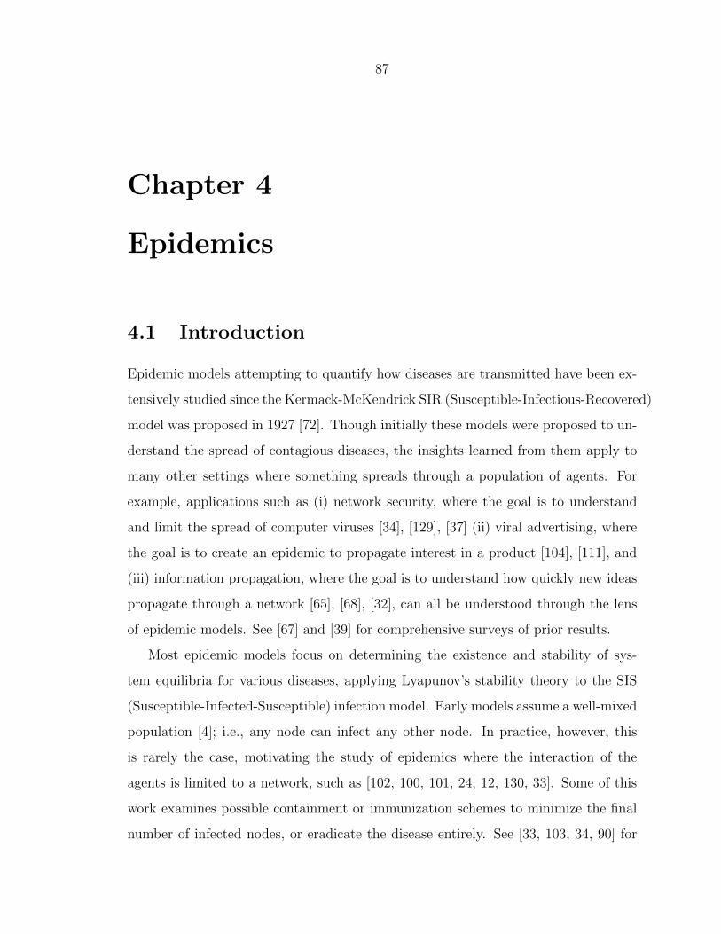
87

Chapter 4

Epidemics

4.1 Introduction

Epidemic models attempting to quantify how diseases are transmitted have been ex-

tensively studied since the Kermack-McKendrick SIR (Susceptible-Infectious-Recovered)

model was proposed in 1927 [72]. Though initially these models were proposed to un-

derstand the spread of contagious diseases, the insights learned from them apply to

many other settings where something spreads through a population of agents. For

example, applications such as (i) network security, where the goal is to understand

and limit the spread of computer viruses [34], [129], [37] (ii) viral advertising, where

the goal is to create an epidemic to propagate interest in a product [104], [111], and

(iii) information propagation, where the goal is to understand how quickly new ideas

propagate through a network [65], [68], [32], can all be understood through the lens

of epidemic models. See [67] and [39] for comprehensive surveys of prior results.

Most epidemic models focus on determining the existence and stability of sys-

tem equilibria for various diseases, applying Lyapunov’s stability theory to the SIS

(Susceptible-Infected-Susceptible) infection model. Early models assume a well-mixed

population [4]; i.e., any node can infect any other node. In practice, however, this

is rarely the case, motivating the study of epidemics where the interaction of the

agents is limited to a network, such as [102, 100, 101, 24, 12, 130, 33]. Some of this

work examines possible containment or immunization schemes to minimize the final

number of infected nodes, or eradicate the disease entirely. See [33, 103, 34, 90] for

88

some of these results. Other work applies techniques from percolation theory to the

SIR model, attempting to answer whether an infection can start from a random node

in a network and infect a giant component of the graph, e.g., [91, 92, 71]. Regardless

of the infection model, most of this work focusses on the long-term behavior of the

system.

Though understanding the extent to which an infection spreads is an important

question in itself, these models can be even more useful in understanding the cost of

an epidemic. Within the medical community, there is a growing trend to quantify

the cost of an epidemic by looking at the direct and indirect medical costs to both

the hospitals and doctors treating and immunizing a population for specific diseases,

as well as the cost to individuals in the population paying for medical care. See [27]

and [117] for two examples of such studies. This interest in cost, both the cost of

disease and the cost of immunization, is the motivation for the current paper. There

is little existing work in the modeling community studying this cost, since any such

calculation depends on the transient behavior of the epidemic model that is often

hard to analyze mathematically. This paper attempts to fill this void.

In this paper, we assume an SIS model of infection, as in [130], [33], and [103], on

a random network that is a variant of the generalized Erdos-Renyi random graph with

arbitrary degree distributions [35, 94] and define the cost or the economic impact of

such an epidemic. Our main contribution is the derivation of (i) the exact cost of an

epidemic in the large graph limit (Theorem 4.1) and (ii) bounds on this cost for a

given graph (Theorem 4.3). We further provide an optimal scheme for random one-

time vaccination, minimizing the total cost of the epidemic, including both disease

and immunization costs. All our results are validated through extensive simulations.

In the derivation of our results, we make use of several techniques from random

matrix theory. We refer the reader to [45, 3] for further details on this subject.

Random matrix theory has found applications in wireless communications [126] and

in the analysis of random graphs [128]. In this paper, we apply ideas from the Stieltjes

transform [126, 125] to analyze the epidemic process on a random network. To the

best of our knowledge, our approach using random matrices is novel to the study of

89

epidemic processes and we hope to extend it in further research.

The paper is organized as follows. We introduce a random network model in

Section 4.2 and the infection process in Section 4.3. Using this framework, we define

and compute the cost of an epidemic in Section 4.4. In Section 4.5, we verify the

assumptions of our model and results through extensive simulations. Finally, we

discuss extensions and conclude in Sections 4.6 and 4.7, respectively.

4.2 Network model

There are two major components to the model studied in this paper: the model of

the underlying network and the model of the infection process. We discuss the model

of the network here and then move to the model of the infection process in the next

section.

Our network model is related to the “configuration” model in [94] and the “general

random graph” model from [35]; however, the model we use is slightly more general

than each.

In particular, let A be an n × n adjacency matrix corresponding to the network,

where there are n nodes in the population and Aij = 1 if there exists a relationship

from node i to node j. For the purposes of this paper, we only consider undirected

graphs; i.e., Aij = Aji. We assume that the network is drawn from a general class of

random graphs, G. For example, the network represented by A could be a realization

of an Erdos-Renyi random graph, Gn,p, which would correspond to allowing each edge

to exist independently with probability p.

The construction of the graph proceeds as follows. First, define a degree distribu-

tion p(·), and obtain n i.i.d. samples w = (w1, . . . , wn). From this vector, generate a

random graph given by the adjacency matrix:

Aij = Aji =

1 w.p. wiwjρ

0 w.p. 1− wiwjρwhere ρ =

1�iwi

. (4.1)

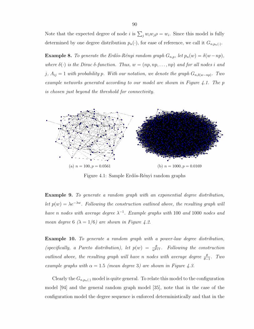
90

Note that the expected degree of node i is�

jwiwjρ = wi. Since this model is fully

determined by one degree distribution pn(·), for ease of reference, we call it Gn,pn(·).

Example 8. To generate the Erdos-Renyi random graph Gn,p, let pn(w) = δ(w−np),

where δ(·) is the Dirac δ-function. Thus, w = (np, np, . . . , np) and for all nodes i and

j, Aij = 1 with probability p. With our notation, we denote the graph Gn,δ(w−np). Two

example networks generated according to our model are shown in Figure 4.1. The p

is chosen just beyond the threshold for connectivity.

(a) n = 100, p = 0.0561 (b) n = 1000, p = 0.0169

Figure 4.1: Sample Erdos-Renyi random graphs

Example 9. To generate a random graph with an exponential degree distribution,

let p(w) = λe−λw. Following the construction outlined above, the resulting graph will

have n nodes with average degree λ−1. Example graphs with 100 and 1000 nodes and

mean degree 6 (λ = 1/6) are shown in Figure 4.2.

Example 10. To generate a random graph with a power-law degree distribution,

(specifically, a Pareto distribution), let p(w) = θ

wθ+1 . Following the construction

outlined above, the resulting graph will have n nodes with average degree θ

θ−1 . Two

example graphs with α = 1.5 (mean degree 3) are shown in Figure 4.3.

Clearly theGn,pn(·) model is quite general. To relate this model to the configuration

model [94] and the general random graph model [35], note that in the case of the

configuration model the degree sequence is enforced deterministically and that in the

91

(a) n = 100 (b) n = 1000

Figure 4.2: Sample exponential random graphs with λ = 16

(a) n = 100 (b) n = 1000

Figure 4.3: Sample power law (Pareto, θ = 1.5) random graphs

general random graph model the expected degree sequence is fixed rather than the

distribution. However, note (like the two models it generalizes) the model we consider

here does not exhibit clustering.

4.3 Infection model

In this section, we describe the infection process that is the focus of this paper.

It is based on the SIS (Susceptible-Infected-Susceptible) epidemic model. In this

formulation, each node in the population transitions between two possible states, i.e.,

susceptible and infected. The process is characterized by two parameters, i.e., δ and

β that represent the recovery rate and the infection rate, respectively. Time is taken

to be discrete and events proceed in each time-step as follows:

92

1. If node i is infected, it recovers with probability δ. Note that it cannot be

infected in the same time-step in which it recovers.

2. If node i is susceptible, it becomes infected by each of its neighbors with i.i.d.

probability β.

In its full generality, this model of SIS infection spread on a network is difficult

to analyze. Thus, it is imperative that we make simplifying approximations to arrive

at a mathematically tractable formulation. To that end, we study a linear infection

spread model commonly used in the literature that was first derived in [130]. We also

describe in detail the sequence of approximations used to derive the linear spread.

First, let us introduce some notation. Consider a graph G on n nodes over which

the epidemic process runs. Let An×n denote its adjacency matrix. Note that the graph

can be one sample of the random graph model presented in the previous section or

it might just be a fixed graph. Define the n× 1 vector P (t) where Pi(t) denotes the

probability that node i is infected at time t. Using this notation, the linear dynamics

of the infection process are given as:

P (t+ 1) =

(1− δ)I� �� �:=M1

+ βA����:=M2

P (t). (4.2)

where I is the n × n identity matrix. The probability of infection at time t + 1

has contributions from two terms, i.e., M1P (t) and M2P (t). The first term is the

contribution from the nodes that are infected at time t and do not recover in the next

time-step with probability 1 − δ. Infected neighbors contributes to the second term

M2P (t) through the adjacency matrix of the graph. Define the system matrix of the

epidemic process as:

M = (1− δ)I + βA (4.3)

Note that in the special case when the infection begins with α-fraction of the

nodes infected at time t = 0, we have P (0) = α1, where ‘1’ denotes an n × 1 vector

93

of all ones. Thus, P (t) can be rewritten as:

P (t) = M tP (0) = αM t1. (4.4)

The above linear system is a commonly adopted approximation for the SIS model

and, has been used in the literature, e.g., in [33, 103, 130].

In this paper, we consider a discrete-time model of the infection process. However,

there is also a large literature that considers continuous-time models, e.g., [101, 102,

24, 12]. Interestingly, the mean field equation describing the system dynamics in

the continuous-time setting is an exact analog of (4.8) and hence the results of our

analysis can be generalized to the continuous-time case.

We now provide a derivation of (4.2) that clearly delineates all the approximations

involved in going from the networked SIS model to the linear system model in (4.2).

Let Ni be the set of neighbors of the i-th node. Consider a sample path s of the

disease propagation. In the sample path s, let P (s)i

(t) denote the probability of node

i being infected at time t in s. We analyze the quantity P (s)i

(t + 1) by conditioning

it on the state of the node i at time t in s. Define the random variable X(s)i(t) as the

number of infected neighbors of i if it is not infected at t in s. If node i is infected at

t in s, we set X(s)i(t) = 0. We conclude from the infection spreading process that the

probability that node i does not get infected at t + 1, given that it was susceptible

at the last time-step, is (1 − β)X(s)i

(t) ≈ 1 − βX(s)i(t). This approximation is valid,

assuming β is small. Thus we can write an expression for P (s)i

(t+ 1) as:

P (s)i

(t+ 1) = (1− δ)P (s)i

(t) + βX(s)i(t)(1− P (s)

i(t)). (4.5)

We take expectation over all sample paths in (4.5) and make use of the fact that Pi(t)

is the expectation of P (s)i

(t) over all sample paths to obtain:

Pi(t+ 1) = (1− δ)Pi(t) + β Es

��1− P (s)

i(t)

�·X(s)

i(t)

�(4.6)

94

Now, we approximate by assuming the terms inside the expectation in (4.6) to be

independent:

Pi(t+ 1) ≈(1− δ)Pi(t) + β(1− Pi(t)) · Es[Xs

i(t)]. (4.7)

Of course the terms inside the expectation in (4.6) are not generally independent.

But, such an approximation may be “reasonable” when the deviations of X(s)i(t) are

not too far from its expectation over all sample paths. One may expect this to be true

for light-tailed degree distributions, but not for heavy-tailed degree distributions.

Now, we evaluate Es[X(s)i(t)]. Note that it is the sum of the probabilities of the

neighbors of node i being infected given that node i itself is susceptible at time t

in s. We approximate this quantity by dropping the conditioning on node i being

susceptible at t in s. This approximation is again valid if the number of infected

neighbors is not too different for nodes that have different degrees. If the degree

distribution is not too heavy-tailed, we expect this to be “reasonable.” Thus, we have

Es[X(s)i(t)] ≈

�j∈Ni

Pj(t). Combining this, we get the following nonlinear recursion:

Pi(t+ 1) ≈ (1− δ)Pi(t) + β(1− Pi(t))�

j∈Ni

Pj(t) (4.8)

We linearize this and express it in matrix-vector form as:

P (t+ 1) ≈ [(1− δ)I + βA]P (t),

Note that the approximations made in the derivation above highlight that we

should not expect the linear system in (4.3) to accurately model SIS infection spread

in all settings. However, it should be a good approximation when the infection rate is

small and when the degree distribution is light-tailed. We should expect the accuracy

to degrade as the infection rate grows or the tail of the degree distribution becomes

heavier. In Section 4.5, we provide simulations to better understand the relationship

of the accuracy of approximation with these parameters of the epidemic model.

95

4.4 Epidemic cost

Given the network and infection models described previously, we can now discuss the

cost of an epidemic on a network. As mentioned previously, a key contribution of

this paper is to provide analytic results characterizing the cost of an epidemic over

its entire lifetime. This includes the effects of the transient behavior of the epidemic,

which is typically difficult to study.

To determine the cost of a disease, we consider a simple model where cd is defined

as the cost of an individual being infected during a single time-step. Thus, cd can

capture both the direct costs to the individual for medication, doctor visits, etc., as

well as secondary costs such as missed work. We note that this model leaves open

the question of how exactly to determine the parameter cd. This is ongoing work

within the medical community; see [27, 117] for example studies in this area. In

future work we expect to incorporate these results to obtain a more accurate cost of

various diseases, but for the purposes of this paper, we leave it as a general parameter

of the model. Note also that this section only concerns the cost of the disease; it

does not include the cost of any strategy to contain or control the epidemic, such as

immunization. In Section 4.6 we discuss minimizing the total cost of both the disease

and the given containment strategy.

Given this model for the cost of disease to an individual, we can formalize the

total social cost of an epidemic. To begin, assume some fraction α < 1 of the nodes

are infected at time t = 0. Denote the epidemic process on a network by the 5-tuple

(G, δ, β,α, cd), where G is the network, δ, β and α define the infection parameters,

and cd defines the cost parameter. Define CD(n), the “disease cost”, as the expected

(averaged over the random spread of the disease) per-node disease cost of an epidemic

during its entire course. Since the infection propagation is stochastic in nature, the

cost for a given tuple (G, δ, β,α, cd) will be a random variable, and CD(n) denotes the

expected value of this quantity when averaged over all infection propagation paths.

To express it in closed form, note that the expected per-node disease cost in a given

time-step t is simply 1TP (t)n

. Furthermore, since P (0) = α1 and P (t) = M t−1P (0),

96

we can express the disease cost per-node as

CD(n) :=1

n

�1T

� ∞�

t=0

M t

�1αcd

�. (4.9)

When the infinite sum converges, i.e., when ||M || < 1, the disease will eventually die

out, and we have

CD(n) =1

nαcd[1

T (I −M)−11]. (4.10)

We emphasize that the above expression is averaged over all possible infection prop-

agation paths, but is a random variable when the underlying network is a random

graph. However, we show that this cost converges almost surely to a deterministic

constant when the network is drawn randomly according to our model (under certain

conditions) and can be explicitly computed.

In Section 4.4.1, we explore the cost in (4.10) in the asymptotic regime, i.e., in the

large graph limit as n → ∞, letting the degree distribution and the infection rate to

vary with the population size. Specifically, the degree distribution for a population

of size n is pn(·) and the infection rate is βn. We compute CD(n) associated with

the epidemic process defined by�Gn,pn(·), δ, βn,α, cd

�. Note that a fixed n is a special

case; i.e., the case where the degree distribution and infection rate do not scale with

n is subsumed in our result. In Section 4.4.3, we provide a bound for the cost of the

disease over a fixed graph. Further, in Section 4.5, we illustrate these results through

extensive simulations.

4.4.1 Asymptotic cost of disease over random graph

In this section, we compute the cost of the epidemic process�Gn,pn(·), δ, βn,α, cd

�,

presenting our result formally in Theorem 4.1.

Let wn×1 be n independent samples drawn according to the degree distribution

pn(·) and W = diag(w). Consider the vector v := βnw. Assume that pn(·) and βn

scale such that the vector v behaves as n independent samples drawn from a scale

invariant distribution p(·) that has a support [vmin,∞), where vmin > 0.

97

Define the following quantities:

V := diag(v) = βnW,

µ :=

�n�

i=1

vi

�−1

,

v := E v =

� ∞

vmin

vp(v)dv,

κ :=1

δ√v

limn→∞

�βn.

Note that if pn(·) and βn do not vary with n then κ > 0. If βn → 0 as n → ∞, then

κ = 0.

Recall that for the random graph model described in Section 4.2, the off-diagonal

entries of the adjacency matrix has mean and variance:

EAij =ρwiwj,

Var Aij =ρwiwj − (ρwiwj)2 ≈ ρwiwj.

where ρ = (1Tw)−1. Define the following n× n matrix C:

C :=1

√nρ

W−1/2�A− ρwwT

�W−1/2 (4.11)

=

�βn

nµV −1/2

�A− µvvT

βn

�V −1/2. (4.12)

It can be verified that C is a standard Wigner matrix [125] where each off-diagonal

98

entry has mean zero and variance 1n. Now define the following n× n matrices:

Y (1)n

:=1

n

�V −1 −

�βn

δ2vC

�−1

, (4.13)

Y (2)n

:=1

n

�I −

�βn

δ2vV 1/2CV 1/2

�−1

(4.14)

Y (3)n

:=1

n

V 1/2

�V −1 −

�βn

δ2vC

�−1

V 1/2

. (4.15)

Using these expressions, we present the technical assumption required for the proof:

Assumption 1. For k = 1, 2, 3, suppose the following holds.

limn→∞

�1T

�Y (k)n

�1− E trY (k)

n

�= 0 a.s. (4.16)

This essentially means that the sum of the off-diagonal entries of the matrices Y (1)n , Y (2)

n

and Y (3)n vanishes in the limit n → ∞.

With this assumption and the notation presented above, we can now state the

main result of this paper that calculates the disease cost CD(n):

Theorem 4.1. For�Gn,pn(·), δ, βn,α, cd

�, if pn(·) has finite variance, the system ma-

trices are almost surely stable for all n, and Assumption 1 holds then

limn→∞

CD(n) =

αcd

δ

�1− v

2

E v2−δv

�a.s if κ = 0,

αcd

δ

�1 + κ2F 2 − κ

2F

2

1−v/F−δκ2v

�a.s if κ �= 0.

where F =

� ∞

vmin

p(v)

v−1 − κ2Fdv.

Before we present the proof, we briefly remark on the assumptions required for

the result to hold. The system matrix M = δI − βnA is assumed to be almost surely

stable. Essentially, this means that the disease dies out with high probability as the

epidemic process proceeds on the random network. If this assumption does not hold,

the cost (CD(n)) is infinite. We also assume the distribution pn(·) has finite variance.

99

To elucidate this assumption, suppose βn = β for all n and the degree distribution

pn(·) is scale invariant. Thus κ > 0. In this regime, most degree distributions that

do not have finite variance are heavy-tailed. It is well known [100] that over most

networks with heavy-tailed degree distributions, there does not exist an infection

threshold in the large-graph limit, i.e., there is no positive ratio of δ/β for which the

infection dies out in these networks. Thus, since we require stability, we need not

consider such networks. However, when the infection and network parameters scale

with n, the connection between stability and finite variance is more involved; hence,

we require the assumption of both finite variance and stability.

For the remainder of this section, we focus on the proof of Theorem 4.1.

4.4.2 Proof of Theorem 4.1

The disease cost in (4.10) can be written as

limn→∞

CD(n) = limn→∞

α

cd

�1T (I −M)−11

�

= limn→∞

αcdn

�1T (δI − βA)−1 1

�

= limn→∞

αcdn

�1T

�δI − βn

√nρW 1/2CW 1/2 − βρwwT

�−11�

= limn→∞

αcdn

1T

δI −�

nβnµV1/2CV 1/2

� �� �:=X

−µvvT

−1

1

= limn→∞

αcdn

�1T

�X − µvvT

�−11�.

Applying the Matrix Inversion Lemma [64], we get

limn→∞

CD(n) = limn→∞

αcdn

�1T

�X−1 − X−1vvTX−1

− 1µ+ vTX−1v

�1

�

= αcd limn→∞

��1

n1TX−11

�−

�1n1TX−1v

�2

− 1nµ

+�1nvTX−1v

��. (4.17)

From the Strong Law of Large Numbers, we have limn→∞ nµ = 1/v almost surely.

To proceed, we show that each of the terms in (4.17), i.e., 1n(1TX−11), 1

n(1TX−1v), and

100

1n(vTX−1v), almost surely self-average under certain technical conditions (Assumption

1) and can be computed easily using pn(·), κ and δ. The result of this computation

is summarized as follows:

Lemma 4.2. If Assumption 1 holds, then

(a) limn→∞

1

n1TX−1v =

F

δa.s. (4.18)

(b) limn→∞

1

n1TX−11 =

1 + κ2F 2

δa.s. (4.19)

(c) limn→∞

1

nvTX−1v =

E v2 a.s. if κ = 0,

1δκ2

�1− v

F

�a.s. if κ �= 0.

(4.20)

where F is the solution of the following fixed point equation:

F =

� ∞

vmin

p(v)

v−1 − κ2Fdv. (4.21)

We defer the proof of Lemma 4.2 to Appendix 4.8. Using this lemma and the fact

that limn→∞ nµ = 1v

a.s. in (4.17), we have, for κ �= 0:

limn→∞

CD(n) = αcd limn→∞

��1

n1TX−11

�−

�1n1TX−1v

�2

− 1nµ

+�1nvTX−1v

��

= αcd

�1 + κ2F 2

δ−

F2

δ2

−v + 1δκ2

�1− v

F

��

a.s.

=αcdδ

�1 + κ2F 2 − κ2F 2

1− v/F − δκ2v

�a.s.

Similarly, the case for κ = 0 follows by substituting the relevant expressions from

Lemma 4.2 in (4.17), which completes the proof.

4.4.3 Bounds for a fixed network

Previously we considered the asymptotic regime for the epidemic process�Gn,pn(·), δ, βn,α, cd

�

and computed the cost exactly for a specific scaling of the parameters. In this section,

we fix the graph and compute the cost of the epidemic process (G, δ, β,α, cd). Since

101

the bound applies to any specific instance of the graph, it also applies to a family of

graphs generated according to the random graph model in Section 4.2.

Theorem 4.3. For (G, δ, β,α, cd), with a stable system matrix M = (1 − δ)I − βA,

the cost of disease per-node satisfies

CD(n) ≤αcd

1− λmax(M)

where λmax(.) denotes the maximum eigenvalue of the corresponding matrix.

Proof. Similarly, let λmin(.) denote the mainimum eigenvalue of a matrix. From

Perron-Frobenius theorem, it follows that

−1 < −λmax(M) ≤ λmin(M) ≤ λmax(M) = |λmax(M)| < 1 (4.22)

Note that (I − M)−1 is a positive definite matrix since all eigenvalues are positive.

From (4.22), we have1

1− λ(M)≤ 1

1− λmax(M)

and

1T (I −M)−11 ≤ 1T�

I

1− λmax(M)

�1 (4.23)

This follows from the fact that if M1 and M2 are positive definite matrices with

eigenvalues λM1 ≤ λM2 for all eigenvalues λM1 and λM2 , then xTM1x ≤ xTM2x for all

x ∈ Rn. The bound follows.

We note that the necessary and sufficient condition required for the disease to die

out and the social cost to converge are the same, i.e., λmax(M) < 1. Also, note that

the bound only depends on λmax(M) from the disease propagation model, which is

popularly known as the disease threshold. It is interesting that the same parameter

of the disease plays the central role in both the tapering off of the disease and its

total cost.

102

4.4.4 Illustration with Erdos-Renyi network

In this section, we illustrate our results using a specific type of network — the Erdos-

Renyi random graph. As described in Example 8, in this type of network, an edge

exists between each pair of nodes with uniform probability p. To generate this graph

using our network model, the degree distribution pn(·) is a delta function at np. It is

well known that such graphs are connected with high probability if p > log n/n in the

large-graph regime [35]. We study the cost of disease in this type of network when

the infection rate βn scales such that βnnp is a constant. Since we are interested in

the regime np → ∞, the infection rate satisfies βn → 0 and κ = 0 in this case. The

scale invariant distribution pn(·) satisfies:

p(v) = δ(v − βnnp),

E v = v = βnnp,

E v2 = (βnnp)2.

We refer to the constant βnnp as v. Using this notation, Theorem 4.1 yields

limn→∞

CD(n) =αcdδ

�1− v2

E v2 − δv

�a.s.

=αcdδ

�1− v2

v2 − δv

�a.s.

=αcdδ − v

a.s. (4.24)

Note that this is essentially the same result as in [17], but applied to the case where the

network and infection parameters scale with n and using slightly different notation.

Now we illustrate the bound in Theorem 4.3 using this class of networks. Consider

a randomly sampled Erdos-Renyi graph with a reasonably large population size n and

edge-forming probability p. To ensure connectedness with high probability, p is chosen

to be greater than log n/n. The infection parameters δ and β are selected such that

δ > βnp. As a result, the maximum eigenvalue of the adjacency matrix of this graph

103

(λmax[A]) is np [35]. Thus we have

λmax(M) = 1− δ + βnp w.h.p.

where w.h.p. denotes “with high probability.” Note that the choice of δ > βnp ensures

that M is stable w.h.p. Using Theorem 4.3, we then have

CD(n) ≤αcd

δ − βnpw.h.p. (4.25)

It is interesting that for an Erdos-Renyi network of large population size the exact cost

in (4.24) as calculated from Theorem 4.1 coincides exactly with the bound in (4.25) as

calculated from Theorem 4.3. This can be explained as follows. For an Erdos-Renyi

network, the adjacency matrix has a large maximum eigenvalue (np) as compared to

the rest of the spectrum that is concentrated in the interval [−2√np, 2

√np] (from

Wigner’s Semicircle Law [125]). The system matrix M has an eigen-spectrum that is

a translation and stretch of the eigen-spectrum of A. Thus it also has the property

that λmax(M) � λ(M), where λ(M) is a randomly sampled eigenvalue of M . The

calculations from Theorem 4.1 and 4.3 coincide since the largest eigenvalue domi-

nates over the other eigenvalues. We illustrate the closeness of the disease cost as

predicted by the two theorems for an Erdos-Renyi network using simulations in the

next section.

4.5 Simulation and discussion

In this section we use simulations to illustrate our results in the previous sections. We

first present simulations in Section 4.5.1 to explore how accurate the linearized model

of epidemic process in (4.2) is when contrasted with the actual disease propagation.

According to our simulations, when the infection rate β is small enough and the

degree distribution pn(.) is not too heavy in its tail, the cost computed via the linear

model of infection spread is a good estimate of the actual disease cost. In the second

part of this section, we illustrate Theorems 4.1 and 4.3 in Section 4.5.2, simulating

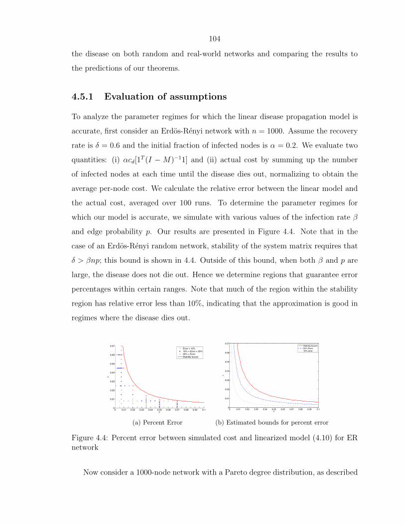
104

the disease on both random and real-world networks and comparing the results to

the predictions of our theorems.

4.5.1 Evaluation of assumptions

To analyze the parameter regimes for which the linear disease propagation model is

accurate, first consider an Erdos-Renyi network with n = 1000. Assume the recovery

rate is δ = 0.6 and the initial fraction of infected nodes is α = 0.2. We evaluate two

quantities: (i) αcd[1T (I − M)−11] and (ii) actual cost by summing up the number

of infected nodes at each time until the disease dies out, normalizing to obtain the

average per-node cost. We calculate the relative error between the linear model and

the actual cost, averaged over 100 runs. To determine the parameter regimes for

which our model is accurate, we simulate with various values of the infection rate β

and edge probability p. Our results are presented in Figure 4.4. Note that in the

case of an Erdos-Renyi random network, stability of the system matrix requires that

δ > βnp; this bound is shown in 4.4. Outside of this bound, when both β and p are

large, the disease does not die out. Hence we determine regions that guarantee error

percentages within certain ranges. Note that much of the region within the stability

region has relative error less than 10%, indicating that the approximation is good in

regimes where the disease dies out.

0 0.01 0.02 0.03 0.04 0.05 0.06 0.07 0.08 0.09 0.10

0.01

0.02

0.03

0.04

0.05

0.06

0.07

p

β

Error < 10%10% < Error < 25%25% < ErrorStability bound

(a) Percent Error

0 0.01 0.02 0.03 0.04 0.05 0.06 0.07 0.08 0.09 0.10

0.01

0.02

0.03

0.04

0.05

0.06

0.07

p

β

Stability bound25% Error10% error

(b) Estimated bounds for percent error

Figure 4.4: Percent error between simulated cost and linearized model (4.10) for ERnetwork

Now consider a 1000-node network with a Pareto degree distribution, as described

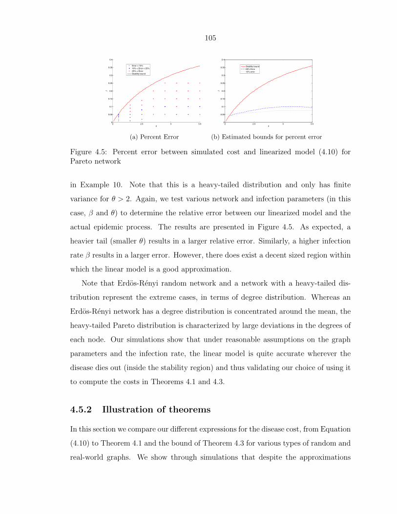
105

2 2.5 3 3.50

0.05

0.1

0.15

0.2

0.25

0.3

0.35

0.4

θ

β

Error < 10%10% < Error < 25%25% < ErrorStability bound

(a) Percent Error

2 2.5 3 3.50

0.05

0.1

0.15

0.2

0.25

0.3

0.35

0.4

θ

β

Stability bound25% Error10% error

(b) Estimated bounds for percent error

Figure 4.5: Percent error between simulated cost and linearized model (4.10) forPareto network

in Example 10. Note that this is a heavy-tailed distribution and only has finite

variance for θ > 2. Again, we test various network and infection parameters (in this

case, β and θ) to determine the relative error between our linearized model and the

actual epidemic process. The results are presented in Figure 4.5. As expected, a

heavier tail (smaller θ) results in a larger relative error. Similarly, a higher infection

rate β results in a larger error. However, there does exist a decent sized region within

which the linear model is a good approximation.

Note that Erdos-Renyi random network and a network with a heavy-tailed dis-

tribution represent the extreme cases, in terms of degree distribution. Whereas an

Erdos-Renyi network has a degree distribution is concentrated around the mean, the

heavy-tailed Pareto distribution is characterized by large deviations in the degrees of

each node. Our simulations show that under reasonable assumptions on the graph

parameters and the infection rate, the linear model is quite accurate wherever the

disease dies out (inside the stability region) and thus validating our choice of using it

to compute the costs in Theorems 4.1 and 4.3.

4.5.2 Illustration of theorems

In this section we compare our different expressions for the disease cost, from Equation

(4.10) to Theorem 4.1 and the bound of Theorem 4.3 for various types of random and

real-world graphs. We show through simulations that despite the approximations

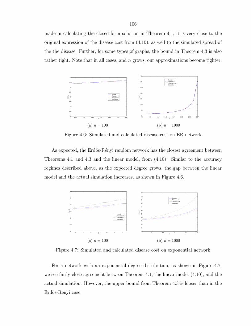
106

made in calculating the closed-form solution in Theorem 4.1, it is very close to the

original expression of the disease cost from (4.10), as well to the simulated spread of

the the disease. Further, for some types of graphs, the bound in Theorem 4.3 is also

rather tight. Note that in all cases, and n grows, our approximations become tighter.

0.01 0.02 0.03 0.04 0.05 0.06 0.070

0.5

1

1.5

2

2.5

3

3.5

4

p

Cd(n

)

InverseTheorem 4.1Theorem 4.3Simulated

(a) n = 100

0 0.01 0.02 0.03 0.04 0.05 0.06 0.070

10

20

30

40

50

60

70

p

Cd(n

)

InverseTheorem 4.1Theorem 4.3Simulated

(b) n = 1000

Figure 4.6: Simulated and calculated disease cost on ER network

As expected, the Erdos-Renyi random network has the closest agreement between

Theorems 4.1 and 4.3 and the linear model, from (4.10). Similar to the accuracy

regimes described above, as the expected degree grows, the gap between the linear

model and the actual simulation increases, as shown in Figure 4.6.

2 4 6 8 10 12 140

1

2

3

4

5

6

µ

Cd(n

)

InverseTheorem 4.1Theorem 4.3Simulated

(a) n = 100

5 10 15 20 250

1

2

3

4

5

6

7

8

9

10

11

µ

Cd(n

)

InverseTheorem 4.1Theorem 4.3Simulated

(b) n = 1000

Figure 4.7: Simulated and calculated disease cost on exponential network

For a network with an exponential degree distribution, as shown in Figure 4.7,

we see fairly close agreement between Theorem 4.1, the linear model (4.10), and the

actual simulation. However, the upper bound from Theorem 4.3 is looser than in the

Erdos-Renyi case.

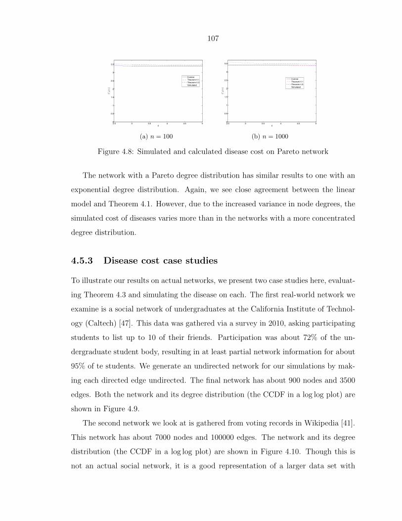
107

2.5 3 3.5 4 4.5 50

0.5

1

1.5

2

2.5

3

3.5

θ

Cd(n

)

InverseTheorem 4.1Theorem 4.3Simulated

(a) n = 100

2.5 3 3.5 4 4.5 50

0.5

1

1.5

2

2.5

3

3.5

θ

Cd(n

)

InverseTheorem 4.1Theorem 4.3Simulated

(b) n = 1000

Figure 4.8: Simulated and calculated disease cost on Pareto network

The network with a Pareto degree distribution has similar results to one with an

exponential degree distribution. Again, we see close agreement between the linear

model and Theorem 4.1. However, due to the increased variance in node degrees, the

simulated cost of diseases varies more than in the networks with a more concentrated

degree distribution.

4.5.3 Disease cost case studies

To illustrate our results on actual networks, we present two case studies here, evaluat-

ing Theorem 4.3 and simulating the disease on each. The first real-world network we

examine is a social network of undergraduates at the California Institute of Technol-

ogy (Caltech) [47]. This data was gathered via a survey in 2010, asking participating

students to list up to 10 of their friends. Participation was about 72% of the un-

dergraduate student body, resulting in at least partial network information for about

95% of te students. We generate an undirected network for our simulations by mak-

ing each directed edge undirected. The final network has about 900 nodes and 3500

edges. Both the network and its degree distribution (the CCDF in a log log plot) are

shown in Figure 4.9.

The second network we look at is gathered from voting records in Wikipedia [41].

This network has about 7000 nodes and 100000 edges. The network and its degree

distribution (the CCDF in a log log plot) are shown in Figure 4.10. Though this is

not an actual social network, it is a good representation of a larger data set with

108

(a) Network

100 101 10210 0.06

10 0.05

10 0.04

10 0.03

10 0.02

10 0.01

Degree

FX(x

)

(b) Degree CCDF

Figure 4.9: Caltech social network

similar characteristics to social networks.

(a) Network

100 101 102 103 104

10 0.015

10 0.013

10 0.011

10 0.009

10 0.007

Degree

FX(x

)

(b) Degree CCDF

Figure 4.10: Wikipedia voting network

Simulating the disease cost on both of these networks, similarly to the method

used for the random networks in the previous section, we see that our model and upper

bound are relatively close to the simulated cost. See Figure 4.11 for the performance

on both the Caltech and Wikipedia social networks. As we do not have access to a p(·)for either of these real networks, we focused on the difference between the upper bound

(Theorem 4.3) and the actual simulation of the disease. Since the Wikipedia network

was rather large, we only plot the upper bound, using the maximum eigenvalue of

the system matrix, for that network.

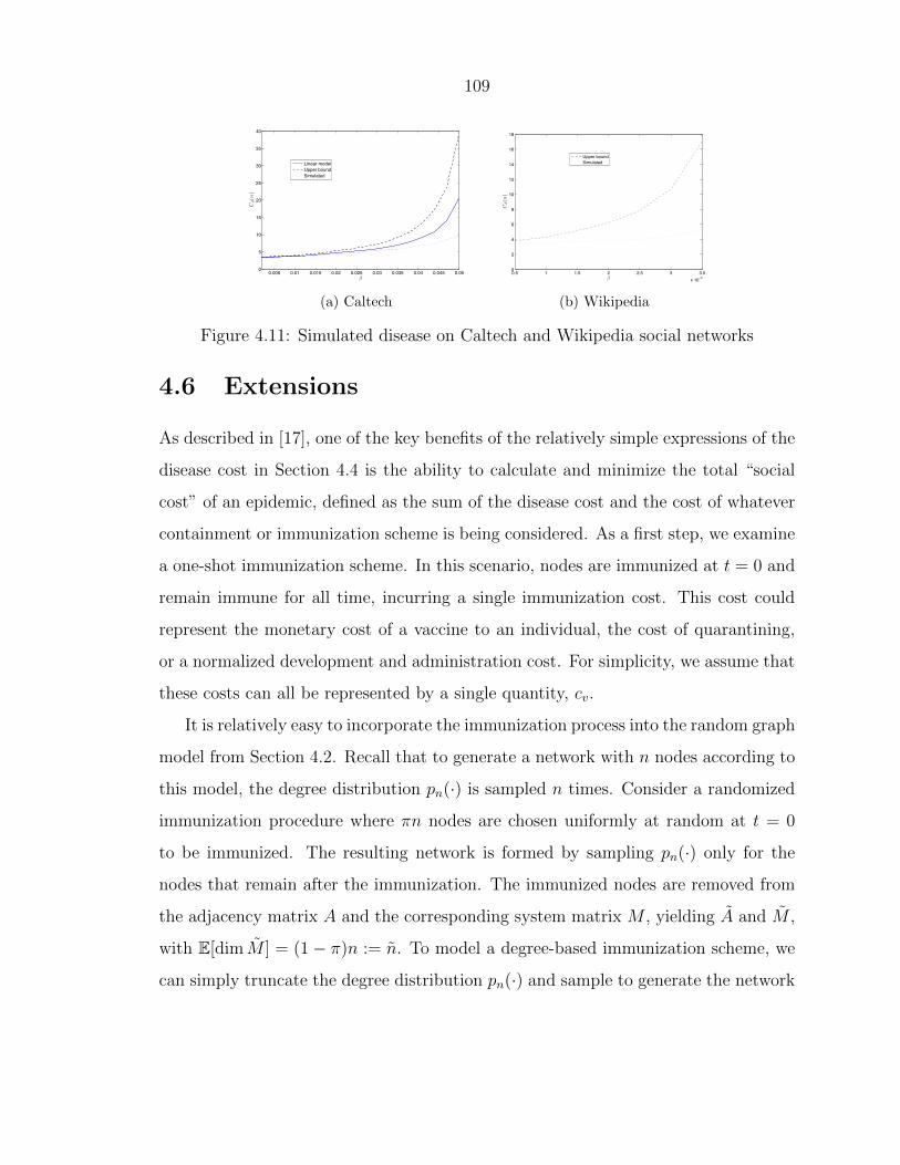
109

0.005 0.01 0.015 0.02 0.025 0.03 0.035 0.04 0.045 0.050

5

10

15

20

25

30

35

40

β

Cd(n

)

Linear modelUpper boundSimulated

(a) Caltech

0.5 1 1.5 2 2.5 3 3.5x 10 3

0

2

4

6

8

10

12

14

16

18

β

Cd(n

)

Upper boundSimulated

(b) Wikipedia

Figure 4.11: Simulated disease on Caltech and Wikipedia social networks

4.6 Extensions

As described in [17], one of the key benefits of the relatively simple expressions of the

disease cost in Section 4.4 is the ability to calculate and minimize the total “social

cost” of an epidemic, defined as the sum of the disease cost and the cost of whatever

containment or immunization scheme is being considered. As a first step, we examine

a one-shot immunization scheme. In this scenario, nodes are immunized at t = 0 and

remain immune for all time, incurring a single immunization cost. This cost could

represent the monetary cost of a vaccine to an individual, the cost of quarantining,

or a normalized development and administration cost. For simplicity, we assume that

these costs can all be represented by a single quantity, cv.

It is relatively easy to incorporate the immunization process into the random graph

model from Section 4.2. Recall that to generate a network with n nodes according to

this model, the degree distribution pn(·) is sampled n times. Consider a randomized

immunization procedure where πn nodes are chosen uniformly at random at t = 0

to be immunized. The resulting network is formed by sampling pn(·) only for the

nodes that remain after the immunization. The immunized nodes are removed from

the adjacency matrix A and the corresponding system matrix M , yielding A and M ,

with E[dim M ] = (1− π)n := n. To model a degree-based immunization scheme, we

can simply truncate the degree distribution pn(·) and sample to generate the network

110

as before. In either case, the social cost of an epidemic can be defined as

S(M, M) :=1

n

�(dimM − dim M)cv +

�1T (I − M)−11

�αcd

�. (4.26)

The second half of the above expression represents the disease cost on the immunized

network and can be calculated using the results in Section 4.4.

In general, any one-shot immunization scheme simply results in a transformation

of pn(·) and the disease cost calculations in Section 4.4 all still apply.

4.6.1 Optimal random immunization

For example, consider the random immunization discussed above. Define the expected

per-node social cost SG(π) on a class of graphs G as a function of the fraction π of

immunized nodes as

SG(π) = πcv + (1− π)CD (n(1− π)) (4.27)

Thus, applying the results from Section 4.4, we can obtain results for SG(π). We

illustrate this with an Erdos-Renyi random network. Using (4.24) from Section 4.4.4

for G = Gn,δ(w−np), we have that, as n → ∞,

SG(π) = πcv +(1− π)αcd

δ − βn(1− π)pw.h.p. (4.28)

We can now determine the optimal fraction of nodes to immunize by minimizing

(4.28). For convenience, we normalize cd = 1 and cv = C, and define a = α

δand

b = αδ

(δ−βnp)2. The optimal fraction of nodes to immunize is then

πopt =

1 C ≤ a < b

1− δ−√

δα/C

βnpa < C < b

0 a < b ≤ C

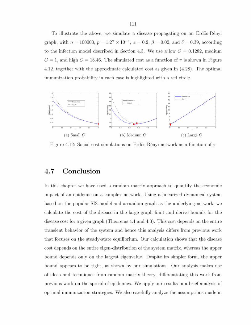
111

To illustrate the above, we simulate a disease propagating on an Erdos-Renyi

graph, with n = 100000, p = 1.27× 10−4, α = 0.2, β = 0.02, and δ = 0.39, according

to the infection model described in Section 4.3. We use a low C = 0.1282, medium

C = 1, and high C = 18.46. The simulated cost as a function of π is shown in Figure

4.12, together with the approximate calculated cost as given in (4.28). The optimal

immunization probability in each case is highlighted with a red circle.

0 0.2 0.4 0.6 0.8 10

0.2

0.4

0.6

0.8

1

1.2

1.4

1.6

π

E[so

cial

cos

t]

Simulation

SG(π)

(a) Small C

0 0.2 0.4 0.6 0.8 10.8

0.9

1

1.1

1.2

1.3

1.4

1.5

1.6

π

E[so

cial

cos

t]

Simulation

SG(π)

(b) Medium C

0 0.2 0.4 0.6 0.8 10

2

4

6

8

10

12

14

16

18

20

π

E[so

cial

cos

t]

Simulation

SG(π)

(c) Large C

Figure 4.12: Social cost simulations on Erdos-Renyi network as a function of π

4.7 Conclusion

In this chapter we have used a random matrix approach to quantify the economic

impact of an epidemic on a complex network. Using a linearized dynamical system

based on the popular SIS model and a random graph as the underlying network, we

calculate the cost of the disease in the large graph limit and derive bounds for the

disease cost for a given graph (Theorems 4.1 and 4.3). This cost depends on the entire

transient behavior of the system and hence this analysis differs from previous work

that focuses on the steady-state equilibrium. Our calculation shows that the disease

cost depends on the entire eigen-distribution of the system matrix, whereas the upper

bound depends only on the largest eigenvalue. Despite its simpler form, the upper

bound appears to be tight, as shown by our simulations. Our analysis makes use

of ideas and techniques from random matrix theory, differentiating this work from

previous work on the spread of epidemics. We apply our results in a brief analysis of

optimal immunization strategies. We also carefully analyze the assumptions made in

112

our linear model and show graph regimes where our assumptions are valid. To the

best of our knowledge, our approach using random matrices is novel to the study of

epidemic processes and we hope to extend it in further research.

To extend this work, we would like to investigate both theoretical and practical

refinements of our model. We can consider more sophisticated epidemic models (SIR,

etc.) as well as immunization based on the strategic behavior of agents. Moreover, a

case study with real data from communicable diseases like influenza or herpes would

provide more insight into the accuracy and predictive power of these models in real-

world scenarios, as well as help refine the cost of disease which we have assumed is a

single parameter, cd.

Our random network approach is a promising direction to tackle the problem

of epidemic spread on network – our simulations show that at least under certain

infection and graph parameters, our results are fairly accurate, giving us hope to

quantify the cost of an epidemic on real-world networks. Our approach and the

random matrix tools we use are fairly general; we hope to extend the tools, techniques

and ideas in this chapter to further study complex processes on complex networks.

4.8 Appendix: Proof of Lemma 4.2

In this section, we prove Lemma 4.2, computing the terms 1n(1TX−1v), 1

n(1TX−11),

and 1n(vTX−1v) in terms of δ, κ and p(v). The calculation relies on techniques from

Random Matrix Theory, specifically the Stieltjes Transform [125]. For the proof, we

require a technical result (Lemma 4.4) that we state and prove in Appendix 4.9. The

computation for the first term, i.e., 1n(1TX−1v) follows directly from Lemma 4.4. For

the other terms, we follow the proof technique of the same lemma and use its result

to finish the proof. Throughout this section, Assumption 1 is supposed to be true.

113

4.8.1 Lemma 4.2 (a)

First we prove that

limn→∞

1

n1TX−1v =

F

δa.s., (4.29)

provided the following condition holds:

limn→∞

1

n

1T�V −1 −

�βn

δ2vC

�−1

1

− 1

nE tr

�V −1 −

�βn

δ2vC

�−1

a.s.. (4.30)

Note that this is the first assumption in Assumption 1. Recall that

F =

� ∞

vmin

p(v)

v−1 − κ2Fdv.

where

κ = limn→∞

�βn

δ2v.

As before, the Strong Law of Large Numbers gives us limn→∞1nµ

= v almost surely.

Substituting the following expression for X in (4.29):

X = δI −�nβnµV

1/2CV 1/2, (4.31)

114

where C is a Wigner matrix and V = diag(v), we obtain

limn→∞

1

n1TX−1v = lim

n→∞

1

n[1TX−1V 1]

= limn→∞

1

n

�1T (δI −

�nβnµV

1/2CV 1/2)−1V 1�

= limn→∞

1

n

�1T (δV −1 −

�nβnµV

−1/2CV 1/2)−11�

= limn→∞

1

n

�1T (δV −1 −

�nβnµC)−11

�

=1

δlimn→∞

1

n

1T�V −1 −

�βn

δ2vC

�−1

1

=1

δlimn→∞

1

nE tr

�V −1 −

�βn

δ2vC

�−1

a.s.

=F

δa.s.,

where the last step follows Lemma 4.4. This completes the proof of Lemma 4.2 (a).

4.8.2 Lemma 4.2 (b)

Now we turn to computing the term 1n1TX−11. We prove that

limn→∞

1

n1TX−11 =

1 + κ2F 2

δa.s. (4.32)

Substituting the expression for X, we have

limn→∞

1

n1TX−11 = lim

n→∞

1

n

�1T

�δI −

�nβnµV

1/2CV 1/2�−1

1

�

=1

δlimn→∞

1

n

1T�I −

�βn

δ2vV 1/2CV 1/2

�−1

1

a.s.

=1

δlimn→∞

1

nE tr

�I −

�βn

δ2vV 1/2CV 1/2

�−1

a.s.

where the last step follows from Assumption 1. Now, we use the same block matrix

decomposition of C and V as in the proof of Lemma 4.4. The definition is restated

115

here.

V =

v1 0

0 V2

and C =

c11 CT

21

C21 C22

,

where v1 and c11 are scalars and the rest are matrices of appropriate sizes. Writing

the matrix using these expressions, we have

�I −

�βn

δ2vV 1/2CV 1/2

�−1

=

1−�

βn

δ2vv1c11 −

�βn

δ2v

√v1CT

21V1/22

−�

βn

δ2v

√v1V

1/22 C21

� �� �:=y

I −�

βn

δ2vV 1/22 C22V

1/22

� �� �:=D

−1

.

Applying the Matrix Inversion Lemma and continuing, we have

limn→∞

E tr1

n

�I −

�βn

δ2vV 1/2CV 1/2

�−1

= limn→∞

E�1−

�βn

δ2vv1c11 − yTD−1y

�−1

= limn→∞

E

1−�

βn

δ2vv1c11 −

βn

δ2vv1C

T

21

�V −12 −

�βn

δ2vC22

�−1

C21

−1

= limn→∞

E

1− βn

δ2vv1C

T

21

�V −12 −

�βn

δ2vC22

�−1

C21

−1

= E�1− κ2v1F

�−1a.s. (4.33)

=

� ∞

vmin

v−1p(v)

v−1 − κ2Fdv a.s..

where we have applied Lemma 4.4 in (4.33). For convenience, define

S1 :=

� ∞

vmin

v−1p(v)

v−1 − κ2Fdv. (4.34)

116

Consider the following relation:

S1 − κ2F 2 =

� ∞

vmin

v−1p(v)

v−1 − κ2Fdv − κ2

� ∞

vmin

Fp(v)

v−1 − κ2Fdv

=

� ∞

vmin

p(v)dv

= 1.

Rearranging and solving for S1 in terms of F , we see that S1 = 1 + κ2F 2 and

limn→∞

1

n1TX−11 =

S1

δ=

1 + κ2F 2

δa.s.,

This proves Lemma 4.2 (b).

4.8.3 Lemma 4.2 (c)

Now we move onto the last term, i.e., we prove that

limn→∞

1

nvTX−1v =

E v2 a.s. if κ = 0,

1δκ2

�1− v

F

�a.s. if κ �= 0.

(4.35)

For brevity, we outline the steps involved.

limn→∞

1

nvTX−1v = lim

n→∞

1

n

�1TV

�δI −

�nβnµV

1/2CV 1/2�−1

V 1

�

=1

δlimn→∞

1

n

1TV 1/2

�V −1 −

�βn

δ2vC

�−1

V 1/21

=1

δlimn→∞

1

nE tr

V 1/2

�V −1 −

�βn

δ2vC

�−1

V 1/2

a.s.

117

where the last step follows from Assumption 1. Using the block-decomposition of C

and V as above, and proceeding as before to expand the above expression, we get

limn→∞

1

nE tr

V 1/2

�V −1 −

�βn

δ2vC

�−1

V 1/2

= limn→∞

E v1

v−11 −

�βn

δ2vc11 −

βn

δ2vCT

21

�V −12 −

�βn

δ2vC22

�−1

C21

−1

= limn→∞

E v1

v−11 − βn

δ2vCT

21

�V −12 −

�βn

δ2vC22

�−1

C21

−1

= E�v1

�v−11 − κ2F

�−1�

a.s. (4.36)

=

� ∞

vmin

vp(v)

v−1 − κ2Fdv a.s..

where we have again applied Lemma 4.4 in (4.36). For convenience, define

S2 :=

� ∞

vmin

vp(v)

v−1 − κ2Fdv. (4.37)

If κ = 0, then

S2 =

� ∞

vmin

v2p(v)dv = E v2.

For the case where κ �= 0, consider the following relation:

F − κ2S2F =

� ∞

vmin

p(v)

v−1 − κ2Fdv −

� ∞

vmin

κ2vFp(v)

v−1 − κ2Fdv

=

� ∞

vmin

vp(v)dw

= v.

Rearranging and solving for S2 in terms of F , we finally have

limn→∞

1

nvTX−1v =

E v2 if κ = 0,

1δκ2

�1− v

F

�if κ �= 0.

118

This proves Lemma 4.2 (c).

4.9 Appendix: Technical proofs

Here we state and prove a technical result used in proving Lemma 4.2. This result

is very similar to the derivation of Wigner’s Semicircle Law using Stieltjes trans-

form in Random Matrix Theory [125]. Our proof technique requires the following

concentration inequality that we state without proof here:

Theorem. Talagrand’s Concentration Inequality: Let K > 0, and let Y1, . . . , Yn be

independent variables with |Yi| ≤ K for all 1 ≤ i ≤ n. Let F : Rn → R be a 1-

Lipschitz conveV function. Then there exists positive constants B, b such that for any

λ,

Pr [|F (Y )−MF (Y )| ≥ λK] ≤ B exp(−bλ2) a.s.,

Pr [|F (Y )− EF (Y )| ≥ λK] ≤ B exp(−bλ2) a.s.,

where M denotes the median.

We first introduce the notation. Let vn×1 be a vector of n independent samples

from a distribution p(.) that has support [vmin,∞). Define the n × n matrix V :=

diag(v). Also, let Cn×n be a Wigner matrix [125] such that all the off-diagonal entries

have mean zero and variance 1/n. Now, consider a sequence {kn}∞n=1 such that it has

a limit, i.e.,

limn→∞

kn = k,

where k is some constant. Using this notation, we present the result:

Lemma 4.4. Let Zn×1 be a vector with independent entries that satisfy EZk = 0,

EZ2k= 1 and the distribution of Zk has bounded support. Then,

limn→∞

1

n

�ZT

�V −1 − knC

�−1Z�− 1

nE tr

�V −1 − knC

�−1= 0 (4.38)

119

and

limn→∞

1

nE tr

�V −1 − knC

�−1= T (k) (4.39)

where T (k) satisfies the following implicit equation:

T (k) =

� ∞

vmin

p(v)dv

v−1 − T (k).

We prove this result through the rest of this section. To begin define the following

function for complex number z:

Tn(z) :=1

nE tr

�V −1 − zC

�−1. (4.40)

We first prove that:

Tn(z)− Tn−1(z) = O�1

n

�.

Now, we prove the claim in (4.38). Note that for a deterministic positive semidef-

inite matrix An×n with operator norm O(1), the function F (V ) = �A1/2V � is convex

and Lipshitz continuous. Then Talagrand’s inequality implies that there exists posi-

tive constants B, b such that for any λ > 0,

Pr���(V TAV )1/2 −M(V TAV )1/2

�� ≥ λ�≤ B exp(−bλ2) a.s.

Thus

(V TAV )1/2 = M(V TAV )1/2 +O(1) a.s.. (4.41)

Now, �V � = O(√n) and hence M(V TAV )1/2 = O(

√n) a.s. On squaring and rear-

ranging (4.41), we have

Pr���V TAV −MV TAV

�� ≥ λ√n�≤ B� exp(−b�λ2)

120

for some positive constants B�, b�. Replacing the median by the expectation, we get

Pr���V TAV − EV TAV

�� ≥ λ√n�≤ B� exp(−b�λ2) (4.42)

If A is a general n×n matrix with operator norm O(1), we can repeatedly use triangle

inequality in (4.42) on the eigen-decomposition of A to get

Pr���V TAV − EV TAV

�� ≥ λ√n�≤ B� exp(−b�λ2)

Now, EV = 0 and the entries are independent. Thus, EV TAV = tr(A). For a random

matrix A independent of V , we can condition on A to get EV TAV = E tr(A) =

nTn(z). Hence,

Pr

�����1

n

�ZT

�V −1 − knC

�−1Z�− Tn(kn)

���� ≥λ√n

�≤ B� exp(−b�λ2).

This gives us

1

n

�ZT

�V −1 − knC

�−1Z�= Tn(kn) +O

�1√n

�. (4.43)

In addition, an application of Borel-Cantelli lemma gives:

limn→∞

1

n

�ZT

�V −1 − knC

�−1Z�− Tn(kn) = 0. a.s. (4.44)

This proves the first claim (4.38) in Lemma 4.4. Now we move to the proof of (4.39).

First, we show that Tn(kn) satisfies an implicit equation and then take limit as n → ∞.

We start with the block matrix decomposition of V and C. Let

V =

v1 0

0 V2

and C =

c11 CT

21

C21 C22

, (4.45)

where v1 and c11 are scalars and the rest are matrices of appropriate sizes. From the

121

Matrix Inversion Lemma [64], it follows that

Tn(kn) =1

nE tr

v−11 − knc11 −knCT

21

−knC21 V −12 − knC22� �� �

=D

−1

=1

nE tr

∆−1 −∆−1CT

21D−1

−D−1C21∆−1 D−1 +D−1C21∆−1CT

21D−1

. (4.46)

where ∆ is the Schur complement of D defined as

∆ = v−11 − knc11 − k2

nCT

21D−1C21. (4.47)

Note that all the diagonal entries of the matrix (V −1 − knC)−1 are identically dis-

tributed. Thus we have

Tn(kn) = E∆−1

= E�v−11 − knc11 − k2

nCT

21D−1C21

�−1

= E�v−11 − CT

21

�V −12 − knC22

�−1C21 +O

�1

n

��−1

.

since c11 has mean zero and variance 1/n. Note that C22

�n

n−1 is a Wigner matrix of

size (n− 1)× (n− 1). Using Z := C21

�n

n−1 in (4.43), we get

CT

21

�V −12 − knC22

�−1C21 =

�n

n− 1

�3/2

Tn−1

�kn

�n

n− 1

�+O

�1√n

�a.s.

=

�n

n− 1

�3/2

Tn

�kn

�n

n− 1

�+O

�1√n

�a.s.

= Tn (kn) +O�

1√n

�a.s..

122

Thus,

Tn(kn) = E�

1

v−11 − k2

nTn(kn)

�+O

�1√n

�

Note that the expectation is over v1 that is drawn according to the distribution p(.).

Taking limit as n → ∞ on both sides

T (k) = E 1

v−1 − k2T (k). (4.48)

The rest follows from (4.44).

123

Chapter 5

Vaccination

5.1 Introduction

Vaccinations are one of the most cost effective ways of preventing disease and promot-

ing health. Yet, vaccination rates for several diseases remains low despite significant

government intervention to promote vaccination coverage. Although some of the

low rates of vaccinations especially in developing countries might be explained by re-

stricted supply or poor availability of health care, lack of demand for vaccinations also

plays an important role ([40]). Recent vaccine scares and subsequent drops in vacci-

nation uptake highlight the importance of this issue in the US and other developed

countries. There is also emerging evidence that individuals might not fully appreci-

ate the costs and benefits of vaccinations when deciding whether or not to vaccinate

([57, 119, 36, 127, 96, 134, 69, 83]). In addition, in our increasingly networked world

with instant access to information and the opinions of others, individuals do not op-

erate in a vacuum; friends’, family, and even strangers’ decisions might influence our

behavior. Therefore, it is imperative to understand how individuals make decisions

regarding vaccinations and the implications of alternate decision models or processes

on the design of efficient public health policy to maximize vaccination coverage and

reduce the burden of vaccine preventable diseases.

In this chapter, we consider two alternate models of the decision to vaccinate. The

models differ in how individuals decision to vaccinate are influenced by the decision

of peers to vaccinate. In particular, we consider two types of peer effects. In the

124

first, rational agents desire to free-ride on the vaccination decisions of their peers. For

example, as an individual sees the overall vaccination coverage of her peers increasing,

she has less desire to vaccinate herself, as there is less and less chance that she will

herself be infected. In this case, peer effects are nonconforming — an increase in

the vaccination coverage by peers leads to a decrease in an individual’s probability of

vaccinating. In the second type of peer effect, agents desire to copy what their peers

are doing, through the simple desire to avoid being different. For example, consider

an agent surrounded by peers who choose not to vaccinate, believing that the vaccine

in question carries a very high risk. Such an agent could face an enormous amount

of peer pressure to conform. As a result, one would expect the desire to copy others’

behavior to play a large role in the vaccination decision-making process. In this case,

peer effects are conforming — an increase in vaccination by peers leads to an increase

in an individual’s probability of vaccinating, and vice versa.

The economics literature on standard models of decision making and discussions

of vaccination decisions consider the positive and normative implications of noncon-

forming peer effects or free-riding ([105]). However, the role of conforming peer effects

has largely been ignored despite a vast literature documenting the existence of con-

forming peer effects in a variety of contexts, such as unhealthy behaviors, academic

achievement and productivity ([118, 84, 48, 55]). In particular, some recent studies

have documented the presence of conforming peer effects in vaccination decisions; see

([60, 61, 87, 99, 109, 121, 124]) for details. In particular, [109] looked at flu vacci-

nation decisions made by undergraduates at a large private university and examined

the role of the social network in health beliefs and vaccination choices. The authors

determine that social effects play a large role in changing people’s perceptions of the

benefits of immunization. Taking advantage of the random assignment of students

to housing, they were further able to show that the clustering of decisions in a social

network were not simply due to homophily, but rather due to positive peer effects on

individuals’ decisions.

In this chapter, we develop a theoretical model based on the standard economic

models of decision-making and incorporate both nonconforming and conforming peer

125

effects. Using this model, we examine how the introduction of peer effects affects

our understanding of the decision to vaccinate and the role of public health policy

in vaccination markets. We note two important related papers here: [52, 14], both

of which model how imitation influences the dynamics of epidemics and vaccination

uptake. In [52], individuals estimate the costs and benefits of vaccination by learn-

ing from others in the population. As agents imitate successful strategies, overall

vaccination coverage drops below even the individual optimum. In [14], the authors

propose a dynamic model in which individuals adopt strategies by imitating others

while considering the current disease prevalence. This model leads to regimes in which

the vaccination uptake oscillates, as is often seen in vaccine scares. The model we

propose in this chapter explicitly examines the role of conforming and nonconforming

peer effects in determining individually optimal strategies. We further build on these

papers and others mentioned above by looking at the role of these peer effects in the

effectiveness of various public health policies.

Overall, our results demonstrate that adding conforming peer effects to the tra-

ditional model of vaccination decisions can have important implications. In the tra-

ditional economic model, agents free-ride on the decisions of others and as a result

the privately optimal vaccination rate is always below the socially optimal vaccina-

tion rate. In contrast, in the model with conforming peer effects privately optimal

vaccination rates can be above or below the social optimal. In the fact the model

produces several evolutionary stable equilibria including no vaccination coverage, full

vaccination coverage and a mixed strategy equilibrium. Traditional models also imply

that vaccine subsidies are always optimal and even large subsidies cannot achieve dis-

ease eradication. In contrast, in the model with conforming peer effects subsidies for

vaccination are not always optimal. However, in certain cases, depending on disease

and vaccine parameters, even small subsidies can achieve disease eradication.

To give a brief overview of this chapter, in Section 5.2, we develop a standard

model of vaccination decisions, where rational economic agents maximize expected

utility or payoffs. We carefully examine the difference between the individually op-

timal strategy and the socially optimal level of vaccination coverage, showing how

126

the parameters of the model will affect the gap between them. We also highlight

the effect of government subsidies on vaccination uptake and how their effectiveness

depends on the cost and risk of the vaccine and disease in question. In Section 5.3

we add conforming peer effects to the standard model and describe the changes in

the individually optimal strategy. With the addition of conforming peer effects, the

individually optimal strategy may lead to a higher level of vaccination coverage that

what is socially optimal — we discuss the implications of this result and its effect on

public policy in the second half of Section 5.3.

5.2 Standard economic model with nonconforming

peer effects

In this section we develop a standard economic model of vaccination decisions, where

rational economic agents maximize expected utility or payoffs, based on the models

in [13, 15]. Vaccination confers immunity against an infectious disease but also may

have adverse health side effects as well as monetary costs. In this model individual

vaccination decisions are linked to decisions of the group as the benefit of vaccina-

tion depends on the prevalence of the infectious disease, which in turn depends on

the group’s likelihood of vaccination. For example, an increase in vaccination rate

among peers would reduce disease prevalence which in turn would reduce individ-

ual incentives to vaccinate. Thus, in the standard economic model, peer effects are

nonconforming — individual decisions are inversely related to group decisions. In

Section 5.3 we add conforming peer effects to the standard model, where an increase

in the group’s likelihood to vaccinate leads to an increase in the individual’s likelihood

to vaccinate. Next, we contrast the normative and positive implications of the two

models.

127

5.2.1 Payoffs

We start with a model of risk-neutral agents with additively separable utility in health

and consumption. Under this model the expected utility from vaccination is given by

Evac = h(H − dv) + u(C −m) (5.1)

where H is an individual’s health endowment, C is consumption, dv is the morbidity

cost of side effects, and m is the marginal cost of producing the vaccine. If agents are

risk-neutral, then the functions h(·) and u(·) are linear and the payoff from vaccination

can be expressed as

Evac = H − dv + θ(C −m) (5.2)

where θ is the marginal utility of consumption in health units.

In the standard economic model with nonconforming peer effects the payoff for

not vaccinating varies only with the infection probability, which depends on the total

vaccination coverage. If agents are risk-neutral, the payoff from not vaccinating can

be expressed as follows,

Env(p) = (H − di)w(p) +H(1− w(p)) + θC (5.3)

= H − diw(p) + θC (5.4)

where di represents the morbidity cost of infection and w(p) is the probability of

being infected when the vaccination coverage is p. We assume that w(p) is strictly

decreasing in p for all p ≤ pcrit. For p ≥ pcrit, w(p) = 0, that is, pcrit is the critical

vaccination threshold above which herd immunity is achieved and the disease erad-

icated. Note that in this model, the cost of not vaccinating only involves a cost of

infection; individuals are fully insured against medical expenses related to treatment

of vaccine preventable disease and face no other monetary or psychological costs of

not vaccinating.

The expected payoff for playing a mixed strategy P (vaccinating with probability

128

P ) when the vaccination coverage level is p is

E[P, p] = P [H + θ(C −m)− dv] + (1− P )[H + θC − diw(p)] (5.5)

= H + θC − P [θm+ dv]− (1− P )[diw(p)] (5.6)

By defining the relative cost as

r = (θm+ dv)/di, (5.7)

this expected payoff can be expressed as

E[P, p] =E[P, p]

di=

H + θC

di− rP − (1− P )[w(p)] (5.8)

where the multiplicative constant di will not make any difference in our proofs or

calculations. With the assumption that 0 ≤ θm+ dv ≤ di, we have 0 ≤ r ≤ 1.

5.2.2 Equilibria

In the vaccination game with nonconforming peer effects, individuals seek to maximize

their expected payoff given the current vaccination coverage p. If p ≥ pcrit, this payoff

function becomes

E[P, p] = H + θC + P [−dv − θm] (5.9)

which is clearly decreasing in P . As a result, if the current vaccination coverage is

above the critical threshold, individuals will always choose to never vaccinate (P =

0). Assuming that the game is played repeatedly (or at least that individuals make

decisions assuming that it is so), this will decrease the total vaccination coverage until

p < pcrit and the probability of infection becomes nonzero.

If p < pcrit, then the expected payoff is given in (5.8). If the payoff function is

decreasing in P , individuals will choose to never vaccinate; if it is increasing in P ,

individuals will choose to always vaccinate. Examining the first case, we see that the

129

payoff function is decreasing in P if r > w(p),

∂E[P, p]

∂P= −r + w(p) < 0. (5.10)

As a result, when r > w(p) individuals will always choose to not vaccinate (P = 0),

decreasing the total vaccination coverage p, and increasing w(p) until the point p∗

where the total vaccination coverage satisfies w(p∗) = r. Note, however, that if

r > w(0), this process will continue to the point where nobody will vaccinate, p = 0.

This is an example of the classic “free-rider” problem, where individuals rationally

choose a strategy where they benefit while not contributing to society, leading to the

point where everyone follows the same strategy and nobody benefits.

In the second case, we see that the payoff function is increasing in P if r < w(p),

∂E[P, p]

∂P= −dv − θm+ diw(p) > 0, (5.11)

As a result, if the relative cost is sufficiently small, individuals will always choose to

vaccinate (P = 1), increasing the vaccination coverage and increasing w(p) until the

point p∗ where the total vaccination coverage satisfies w(p∗) = r. See Figure 5.1 for

an illustration of this solution. This strategy is stable, as stated formally in Lemma

5.1; we leave the detailed proof of this lemma to 5.6.

w(0)  

pcrit  

w(p)  

0   p  1  

1  

r  

p*  

Figure 5.1: Solving r = w(p∗)

130

Lemma 5.1. The mixed strategy p∗ that satisfies w(p∗) = r is a weak Nash Equi-

librium and an Evolutionarily Stable Strategy in the vaccination game with noncon-

forming peer effects if r = θm+dv

di< w(0). If r > w(0), the pure strategy P = 0 is a

strict Nash Equilibrium and Evolutionarily Stable Strategy.

5.2.3 Social welfare and individually optimum strategies

In many games the equilibrium reached by rational agents may not be the socially

optimal value. In our case, we define the social welfare as the normalized total utility

of the population,

W (p) = pEvac + (1− p)Env(p) (5.12)

and using our payoff functions from Section 5.2.1, we have

W (p) = p[H + θ(C −m)− dv] + (1− p)[H + θC − diw(p)]. (5.13)

For a general infection probability function w(p) with vaccination threshold pcrit,

the socially optimal vaccination coverage popt is the vaccination level that maximizes

the social welfare, i.e.,

popt = argmax0≤p≤1

W (p) (5.14)

The social welfare function is decreasing for p > pcrit:

∂W (p)

∂p= −θm− dv < 0 (5.15)

where (5.15) uses the fact that w(p) = 0 for p > pcrit. For p > pcrit, increasing

vaccination rates reduces the social welfare, as the disease is already eradicated and

increasing vaccinations provide no benefit but individuals incur the monetary costs

of the vaccine.

For p < pcrit, differentiating with respect to p, we have

∂W (p)

∂p= −θm− dv + di

�w(p)− (1− p)

∂w(p)

∂p

�(5.16)

131

where ∂w(p)∂p

< 0 for 0 < p < pcrit. As a result, the social welfare function is increasing

in p for p ≤ pcrit if

θm+ dv < di

�w(p)− (1− p)

∂w(p)

∂p

�(5.17)

or equivalently, if

r < w(p)− (1− p)∂w(p)

∂p. (5.18)

If this condition is met, the maximum social welfare will be achieved at popt = pcrit,

the point at which the disease is eradicated. If this condition is not met, we have

popt ≤ pcrit, since the social welfare function is always decreasing beyond pcrit.

Remark 1. Note that from a policy perspective, often the desired vaccination level

is one that achieves herd immunity or disease eradication, so popt = pcrit, regardless

of wherever the minimum of the social welfare function might be. For example, in

1977 the World Health Organization (WHO) successfully eradicated smallpox through

a worldwide vaccination program [49]. The rationale is that disease eradication ben-

efits not only the current generation but also future generations. The social welfare

function we consider in this chapter only models the welfare of the current generation

and therefore within the context of our model popt can be lower than pcrit.

Remark 2. As a running example throughout this chapter, we will consider the in-

fection probability w(p) as the steady-state infection probability in a SIR (Susceptible-

Infected-Recovered) model with constant birth and death rate µ. In this case, w(p) =

1 − 1R0(1−p) where R0 is the reproduction ratio of the disease in question. For a de-

tailed description of this model and how to derive its infection probability function,

see 5.7. For this model, the disease will be eradicated if the vaccination level is at

or above the critical vaccination threshold: pcrit = 1 − 1/R0. In this example, the

optimal vaccination coverage will be popt = pcrit, as the condition in (5.18) is satisfied

for w(p) = 1− 1R0(1−p) , as long as r < 1, which is true by assumption.

However, if we assume that individuals are allowed to make their own vaccination

decisions, disease eradication will not be possible, and often the optimal vaccination

coverage is not acheived. The privately optimal strategy p∗ is always less than the

132

critical vaccination threshold, as shown in Figure 5.1. Even in the case where the so-

cially optimal vaccination rate is less than the critical threshold, the privately optimal

strategy is still less than the social optimum. Formally,

Theorem 5.2. The private optimum p∗ ≤ popt in the vaccination game with noncon-

forming peer effects.

Proof. Differentiating the social welfare function when p < pcrit, we have

∂W (p)

∂p= [−dv − θm+ diw(p)] + (1− p)

�−di

∂w(p)

∂p

�(5.19)

=∂E[P, p]

∂P+ (1− p)

�−di

∂w(p)

∂p

�

� �� �>0 always, since ∂w(p)

∂p<0

(5.20)

The first term captures the private benefit from increasing vaccination and the second

term captures the societal benefit which arises as increasing vaccination reduces the

probability of infection for the entire population. At the private optimum p = p∗,

the social welfare will be increasing with p, since ∂E[P,p]∂P

= 0 for p = p∗. Further, for

p < p∗, the social welfare will also be increasing with p, as

−dv − θm+ diw(p− �) > −dv − θm+ diw(p∗) = 0 (5.21)

where the inequality comes from the fact that w(p) is decreasing in p. So, the

social welfare function is increasing in p for all p ≤ p∗, and as a result, since

popt = argmaxW (p) and using the analysis above, we have

p∗ ≤ popt ≤ pcrit (5.22)

Exactly how much lower the social welfare is when individuals act selfishly from the

optimal point depends on several factors. The social welfare at the socially optimal

point, dividing by the constant di to obtain an expression in terms of the relative

133

cost, is

W (popt)

di=

1

di(popt[H + θ(C −m)− dv] + (1− popt)[H + θC − diw(popt)]) (5.23)

=H + θC

di− w(popt) + popt[−r + w(popt)]. (5.24)

The social welfare at the private optimum, again dividing by di, is

W (p∗)

di=

1

di(p∗[H + θ(C −m)− dv] + (1− p∗)[H + θC − diw(p

∗]) (5.25)

=H + θC

di− w(p∗) + p∗[−r + w(p∗)] (5.26)

=H + θC

di− w(p∗) (5.27)

since w(p∗) = r. We can easily calculate the difference between the two:

W (popt)−W (p∗)

di=

H + θC

di− w(popt) + popt[−r + w(popt)]−

H + θC

di+ w(p∗)

(5.28)

= (1− popt)(r − w(popt)) (5.29)

again using w(p∗) = r. The above equations show that as the cost of the vaccine

(m and dv) increases and as the cost of infection (di) decreases, this gap in welfare

will increase; fewer people will voluntarily choose to vaccinate and the social welfare

will decrease. We can lower bound the difference, relating it to the social welfare at

the point where the disease is eradicated. This lower bound is less meaningful if the

optimum vaccination rate is exactly the critical threshold.

5.2.4 Effect of government subsidies

If the government offers subsides of the monetary cost of the vaccine, individuals’

expected payoff for vaccinating becomes a function of the subsidy:

Evac(s) = H + θ(C −m(1− s))− dv (5.30)

134

where s represents the percentage of the marginal production cost of the vaccine that

the government is subsidizing. The private optimum, as a function of the subsidy,1

becomes

p∗(s) = w−1

�θm(1− s) + dv

di

�. (5.31)

Note that this function is strictly decreasing in its argument, since the original proba-

bility of infection function w(p) is also strictly decreasing. In general, the effectiveness

of the subsidy is inversely related to the morbidity cost of the disease, di. That is,

vaccine subsidies are less effective for more deadly diseases. However, the effectiveness

of the subsidy is directly related to the morbidity (and monetary) cost of the vaccine,

dv — the vaccine subsides are more effective for more dangerous vaccines. Looking at

(5.31) more closely, we see that it is an increasing function of s and di, but decreasing

in m and dv. Intuitively, as the government subsidy increases and lowers the mone-

tary cost of the vaccine (or as the danger of infection increases), more people will be

inclined to buy the vaccine. Similarly, as the cost and risk of the vaccine increases,

less people will be inclined to vaccinate.

Continuing with our running example, we examine the private optimum as a

function of the subsidy for a specific infection probability function w(p) = 1− 1R0(1−p) .

In this case, the private optimum becomes

p∗(s) = 1− 1

R0

�1− θm(1−s)+dv

di

� (5.32)

and the derivative with respect to s is

∂p∗(s)

∂s=

θm

diR0

�1− θm(1−s)+dv

di

�2 . (5.33)

Inspecting the above equation, we can see that the effectiveness of the subsidy will

be higher for a higher cost and higher risk (larger m and dv) vaccine, whereas for a

more dangerous disease (larger di) the subsidy will not be as effective.

1Recall that the private optimum when subsidies are not present is p∗ = w−1�

θm+dvdi

�.

135

Let x(s) = θm(1−s)+dv

dito simplify notation. If the goal is to eradicate the disease,

then we need x(s) = 0 so that p∗(s) = pcrit. The subsidy that achieves disease

eradication even when individuals behave selfishly is

sopt = 1 +dvθm

(5.34)

obtained by setting x(s) = 0. Note that the optimal subsidy here is greater than

one — the subsidy must compensate individuals for more than just the monetary

cost of the vaccine in order to eradicate the disease. If we impose the constraint that

0 ≤ s ≤ 1, the optimal subsidy will be exactly sopt = 1.

The social welfare function, as a function of the subsidy, is

W (p∗(s)) = p∗(s)[H + θ(C −m)− dv] + (1− p∗(s))[H + θC − diw(p∗(s))] (5.35)

When s = sopt, this simplifies to

W (p∗(sopt)) = pcrit[H + θ(C −m)− dv] + (1− pcrit)[H + θC] (5.36)

= H + θ(C − pcritm)− pcritdv. (5.37)

In contrast, if we look at the social welfare function when there is no subsidy and

individuals behave selfishly, we have

W (p∗) = p∗[H + θ(C −m)− dv] + (1− p∗)[H + θC − diw(p∗)] (5.38)

= H + θ(C −m)− dv (5.39)

which is always less than the social welfare at the optimum. Further, it is easy to

show that W (p∗(s)) > W (p∗) for any s > 0.

136

5.3 Standard economic model with conforming and

nonconforming peer effects

In this section we add conforming peer effects to the standard model in Section 5.2,

demonstrating the interaction between the desire to behave rationally and the desire

to conform to what others are doing. We follow the same format as in the previous

section, first describing the payoffs and equilibria of the model and then discussing

the differences between the individually optimal strategies and the socially optimal

vaccination coverage, as well as the effect of government subsidies in this new, more

realistic model of human decisions.

5.3.1 Payoffs

We begin by defining payoff functions for following each strategy: vaccinating and

not vaccinating. We use a linear combination of the payoff functions from Section 5.2

and new payoff functions capturing the reward one gets by conforming:

Evac(p) = γ�f(p) +H − dv + θ(C −m) (5.40)

Env(p) = γ�g(p) +H − diw(p) + θC (5.41)

where γ� ∈ (0,∞] measures the strength of the desire to conform, f(p) is a strictly

increasing function representing the desire to conform to the vaccinating strategy, and

g(p) is a strictly decreasing function representing the desire to conform to the nonvac-

cinating strategy. Note that this general formulation can capture bias; for example, a

given population might put more weight on conforming to the nonvaccinating, rather

than vaccinating, strategy. All other variables are the same as defined in Section 5.2.

We can also describe a simpler game with symmetric linear payoff functions for

137

conformity, as follows. Let f(p) = p and g(p) = 1− p, so that

Evac(p) = γ�p+H − dv + θ(C −m) (5.42)

Env(p) = γ�(1− p) +H − diw(p) + θC (5.43)

The expected payoff for playing a mixed strategy P (vaccinating with probability

P ) when the vaccination coverage level is p is

E[P, p] = P [γ�f(p) +H + θ(C −m)− dv] + (1− P )[γ�g(p) +H + θC − diw(p)]

(5.44)

= H + θC − P [θm+ dv − γ�f(p)]− (1− P )[diw(p)− γ�g(p)] (5.45)

Again dividing through by di and using the relative cost of the vaccine, we can express

the expected payoff as

E[P, p] =E[P, p]

di=

H + θC

di− P [r − γf(p)]− (1− P )[w(p)− γg(p)] (5.46)

where γ = γ�

diis just a scaled constant measuring the strength of the desire to conform.

Note that we retain the assumption that 0 ≤ r ≤ 1. For convenience, let h(p) =

g(p)− f(p), a useful strictly decreasing summary function. We assume

h(0) = α (5.47)

h(1) = −β. (5.48)

For reference, we also define the pure conformity game, where payoffs are only

a function of the desire to conform to others, and there are no nonconforming peer

effects.

Evac(p) = γ�f(p) (5.49)

Env(p) = γ�g(p) (5.50)

138

The pure conformity game has two pure strict NE (and ESS’s): P = 0 and P = 1,

which can easily be shown to always exist. It further has a weak NE at P = p∗ where

p∗ is the solution to 0 = γ�h(p∗), but this equilibria is not an ESS. If we use the

symmetric linear conformity payoff functions as described in (5.42) and (5.43), we

have

Evac(p) = γ�p (5.51)

Env(p) = γ�(1− p) (5.52)

This simple pure conformity game will always have two pure strict NE (and ESS’s):

P = 0 and P = 1. It also has a weak NE at P = p∗ = 1/2, where p∗ is the solution to

0 = h(p∗) = γ�(1−2p∗), but this equilibria will not be an ESS. To illustrate this result,

imagine the conformity game with exactly half of the population vaccinating. As soon

as the fraction vaccinating slightly increases (or decreases), the majority strategy is

no longer 50—50, and the population will converge to the strict NE P = 1, always

vaccinating (or P = 0, never vaccinating).

5.3.2 Equilibria

Just as described in Section 5.2.2, individuals here will seek to maximize their ex-

pected payoff given the current vaccination coverage p. However, when the game

also includes conforming peer effects, individual strategies become more complicated,

reflecting the tension between the desire to conform and to free-ride on others’ de-

cisions to vaccinate. In this section, we show that the vaccination game with both

conforming and nonconforming peer effects can have multiple stable equilibria whose

existence and stability depend on the disease and cost parameters of the model, in

contrast to the vaccination game with only nonconforming peer effects, which only

has one stable equilibrium.

Lemma 5.3. The pure nonvaccinating strategy P = 0 is a strict Nash Equilibrium

and Evolutionarily Stable Strategy of the vaccination game with conforming and non-

139

conforming peer effects if r > w(0)− γα.

Proof. Using Definition 7 from 5.5, the pure strategy P = 0 (never vaccinating) is

a strict Nash Equilibrium (and thus an evolutionarily stable strategy) if E(P, P ) −E(Q,P ) > 0. Calculating this, we have

E(P, P )− E(Q,P ) = (P −Q)(Ev(P )− Env(P )) (5.53)

= −Q(Ev(0)− Env(0)) (5.54)

= −Q(−θm− dv + diw(0)− γ�α) (5.55)

Thus, E(P, P ) > E(Q,P ) and P = 0 is a strict NE and ESS if

−θm− dv + diw(0)− γ�α < 0, (5.56)

or equivalently, if r > w(0)− γα.

The above lemma states that if the vaccine is sufficiently costly or has large side

effects relative to the mortality costs of infection, never vaccinating will be a stable

equilibrium strategy. Alternatively, if the disease is sufficiently not infectious, that

is, w(0) is small, then never vaccinating will be a stable equilibrium strategy. Note

that as γ → 0 and the desire to conform goes away, this approaches the condition for

never vaccinating when only nonconforming peer effects are present. However, when

γ → ∞, and the conforming strategy dominates, never vaccinating will always be a

stable equilibrium strategy, as in the pure conformity game.

Lemma 5.4. The pure vaccinating strategy P = 1 is a strict Nash Equilibrium and

Evolutionarily Stable Strategy of the vaccination game with conforming and noncon-

forming peer effects if r < γβ.

Proof. Using Definition 7 from 5.5, the pure strategy P = 1 (always vaccinating) is

a strict Nash Equilibrium (and thus an evolutionarily stable strategy) if E(P, P ) −

140

E(Q,P ) > 0. Calculating this, we have

E(P, P )− E(Q,P ) = (P −Q)(Ev(P )− Env(P )) (5.57)

= (1−Q)(Ev(1)− Env(1)) (5.58)

= (1−Q)(−θm− dv + γ�β) (5.59)

since w(1) = 0. Thus, E(P, P ) > E(Q,P ) and P = 1 is a strict NE and ESS if

−θm− dv + γ�β > 0, (5.60)

or equivalently, if r < γβ.

The above lemma states that if the vaccine is sufficiently safe, always vaccinating

will be a stable equilibrium strategy. Note that as γ → 0 and the desire to conform

goes away, always vaccinating will never be a stable equilibrium, as is the case for the

vaccination game with only nonconforming peer effects. However, when γ → ∞, and

the conforming strategy dominates, always vaccinating becomes a stable equilibrium

strategy, as in the pure conformity game.

Lemma 5.5. The mixed strategy p∗ satisfying Ev(p∗) = Env(p∗) is a weak Nash Equi-

librium and Evolutionarily Stable Strategy for the vaccination game with conforming

and nonconforming peer effects if

∂w(p)

∂p< γ

∂h(p)

∂p(5.61)

Proof. Consider a population following the mixed equilibrium strategy p∗, (vaccinat-

ing with probability p∗) where p∗ is the solution to the equation

Ev(p∗) = Env(p

∗) (5.62)

141

This strategy is clearly a weak Nash Equilibrium, since

E(p∗, p∗)− E(Q, p∗) = (p∗ −Q)(Ev(p∗)− Env(p

∗)) = 0. (5.63)

Using Definition 9 from 5.5, p∗ will be an evolutionarily stable strategy if

E(p∗, Q) > E(Q,Q) ⇐⇒ (p∗ −Q)(Ev(Q)− Env(Q)) > 0. (5.64)

This definition states that vaccinating with probability p∗ is preferable to some other

level Q, given that the current vaccination coverage isQ— the equilibrium strategy p∗

will be able to successfully “invade” a population with coverage Q. It turns out that

p∗ will be an ESS if Ev(p)− Env(p) is strictly decreasing in the vaccination coverage

p. To see this, consider first the case where Q > p∗, where the current vaccination

coverage is greater than the equilibrium p∗. If Ev(p) − Env(p) is strictly decreasing

in the vaccination coverage p, then

Ev(Q)− Env(Q) < Ev(p∗)− Env(p

∗) = 0 (5.65)

and so we have (p∗ − Q)(Ev(Q) − Env(Q)) > 0, and individuals vaccinating with

probability p∗ will obtain a higher expected payoff than the rest of the population

when the coverage level Q is greater than p∗.

Now consider the case where Q < p∗, where the current vaccination coverage is

less than the equilibrium p∗. Again, if Ev(p) − Env(p) is strictly decreasing in the

vaccination coverage p, then

Ev(Q)− Env(Q) > Ev(p∗)− Env(p

∗) = 0 (5.66)

and so we have (p∗ − Q)(Ev(Q) − Env(Q)) > 0, and individuals vaccinating with

probability p∗ will obtain a higher expected payoff than the rest of the population.

Thus, individuals vaccinating with probability p∗ solving Ev(p∗) = Env(p∗) will

have higher expected payoffs than the rest of the population when the vaccination

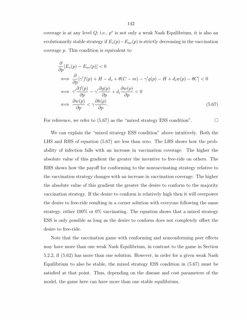
142

coverage is at any level Q; i.e., p∗ is not only a weak Nash Equilibrium, it is also an

evolutionarily stable strategy if Ev(p)−Env(p) is strictly decreasing in the vaccination

coverage p. This condition is equivalent to

∂

∂p[Ev(p)− Env(p)] < 0

⇐⇒ ∂

∂p[γ�f(p) +H − dv + θ(C −m)− γ�g(p)−H + diw(p)− θC] < 0

⇐⇒ γ�∂f(p)

∂p− γ�∂g(p)

∂p+ di

∂w(p)

∂p< 0

⇐⇒ ∂w(p)

∂p< γ

∂h(p)

∂p. (5.67)

For reference, we refer to (5.67) as the “mixed strategy ESS condition”.

We can explain the “mixed strategy ESS condition” above intuitively. Both the

LHS and RHS of equation (5.67) are less than zero. The LHS shows how the prob-

ability of infection falls with an increase in vaccination coverage. The higher the

absolute value of this gradient the greater the incentive to free-ride on others. The

RHS shows how the payoff for conforming to the nonvaccinating strategy relative to

the vaccination strategy changes with an increase in vaccination coverage. The higher

the absolute value of this gradient the greater the desire to conform to the majority

vaccination strategy. If the desire to conform is relatively high then it will overpower

the desire to free-ride resulting in a corner solution with everyone following the same

strategy, either 100% or 0% vaccinating. The equation shows that a mixed strategy

ESS is only possible as long as the desire to conform does not completely offset the

desire to free-ride.

Note that the vaccination game with conforming and nonconforming peer effects

may have more than one weak Nash Equilibrium, in contrast to the game in Section

5.2.2, if (5.62) has more than one solution. However, in order for a given weak Nash

Equilibrium to also be stable, the mixed strategy ESS condition in (5.67) must be

satisfied at that point. Thus, depending on the disease and cost parameters of the

model, the game here can have more than one stable equilibrium.

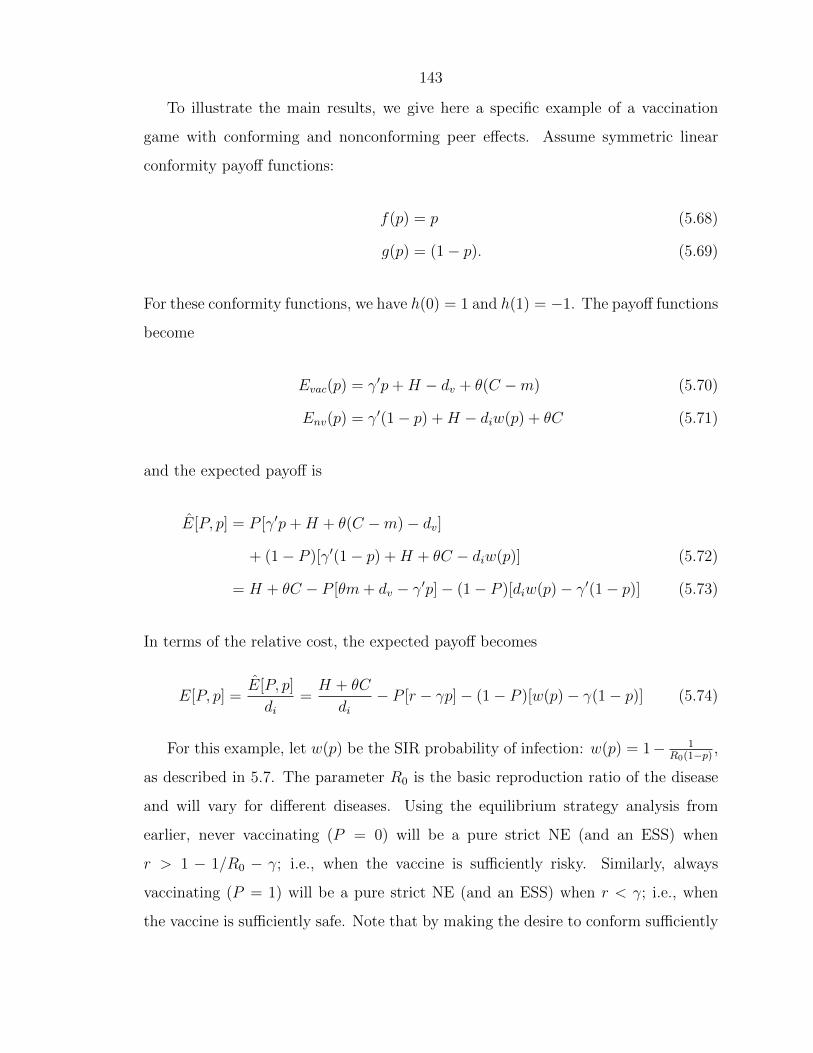
143

To illustrate the main results, we give here a specific example of a vaccination

game with conforming and nonconforming peer effects. Assume symmetric linear

conformity payoff functions:

f(p) = p (5.68)

g(p) = (1− p). (5.69)

For these conformity functions, we have h(0) = 1 and h(1) = −1. The payoff functions

become

Evac(p) = γ�p+H − dv + θ(C −m) (5.70)

Env(p) = γ�(1− p) +H − diw(p) + θC (5.71)

and the expected payoff is

E[P, p] = P [γ�p+H + θ(C −m)− dv]

+ (1− P )[γ�(1− p) +H + θC − diw(p)] (5.72)

= H + θC − P [θm+ dv − γ�p]− (1− P )[diw(p)− γ�(1− p)] (5.73)

In terms of the relative cost, the expected payoff becomes

E[P, p] =E[P, p]

di=

H + θC

di− P [r − γp]− (1− P )[w(p)− γ(1− p)] (5.74)

For this example, let w(p) be the SIR probability of infection: w(p) = 1− 1R0(1−p) ,

as described in 5.7. The parameter R0 is the basic reproduction ratio of the disease

and will vary for different diseases. Using the equilibrium strategy analysis from

earlier, never vaccinating (P = 0) will be a pure strict NE (and an ESS) when

r > 1 − 1/R0 − γ; i.e., when the vaccine is sufficiently risky. Similarly, always

vaccinating (P = 1) will be a pure strict NE (and an ESS) when r < γ; i.e., when

the vaccine is sufficiently safe. Note that by making the desire to conform sufficiently

144

strong (increasing γ), we can achieve the same result. All solutions2 to the equation

Evac(p∗) = Env(p

∗) (5.75)

will be weak Nash Equilibria for this example. For p < pcrit this becomes

γ�p∗ +H − dv + θ(C −m) = γ�(1− p∗) +H − di

�1− 1

R0(1− p∗)

�+ θC

−r = γ(1− 2p∗)−�1− 1

R0(1− p∗)

�. (5.76)

However, only one solution of (5.75) will satisfy the mixed strategy ESS condition in

(5.67). This solution is given by

q∗ =

√R0(3γ + r − 1) +

�R0(γ − r + 1)2 − 8γ

4√R0γ

. (5.77)

This solution will exist when

0 ≤ γ ≤ r

1− 2R0

(5.78)

or, in terms of r, when

γ

�1− 2

R0

�≤ r ≤ 1 + γ − 2

√2

�γ

R0. (5.79)

Note that as q∗ is the solution to the quadratic equation, it will by necessity always

be less than pcrit. We plot all of the evolutionarily stable strategies for this example

as a function of γ in Figure 5.2, with R0 = 5 and r = 0.5. The solid black horizontal

line shows the vaccination coverage needed to eradicate the disease. Examining the

2There are three solutions to the equation in (5.75), two to the quadratic equation (5.76) andone to the linear equation which occurs when p ≥ pcrit and w(p) = 0. They are given by

q1,2 =

√R0(3γ + r − 1)±

�R0(γ − r + 1)2 − 8γ

4√R0γ

l =γ + r

2γ

Using the mixed ESS condition in (5.67) we see that the linear solution l will never be an ESS, andwhen the quadratic solutions exist, only q1 will be an ESS.

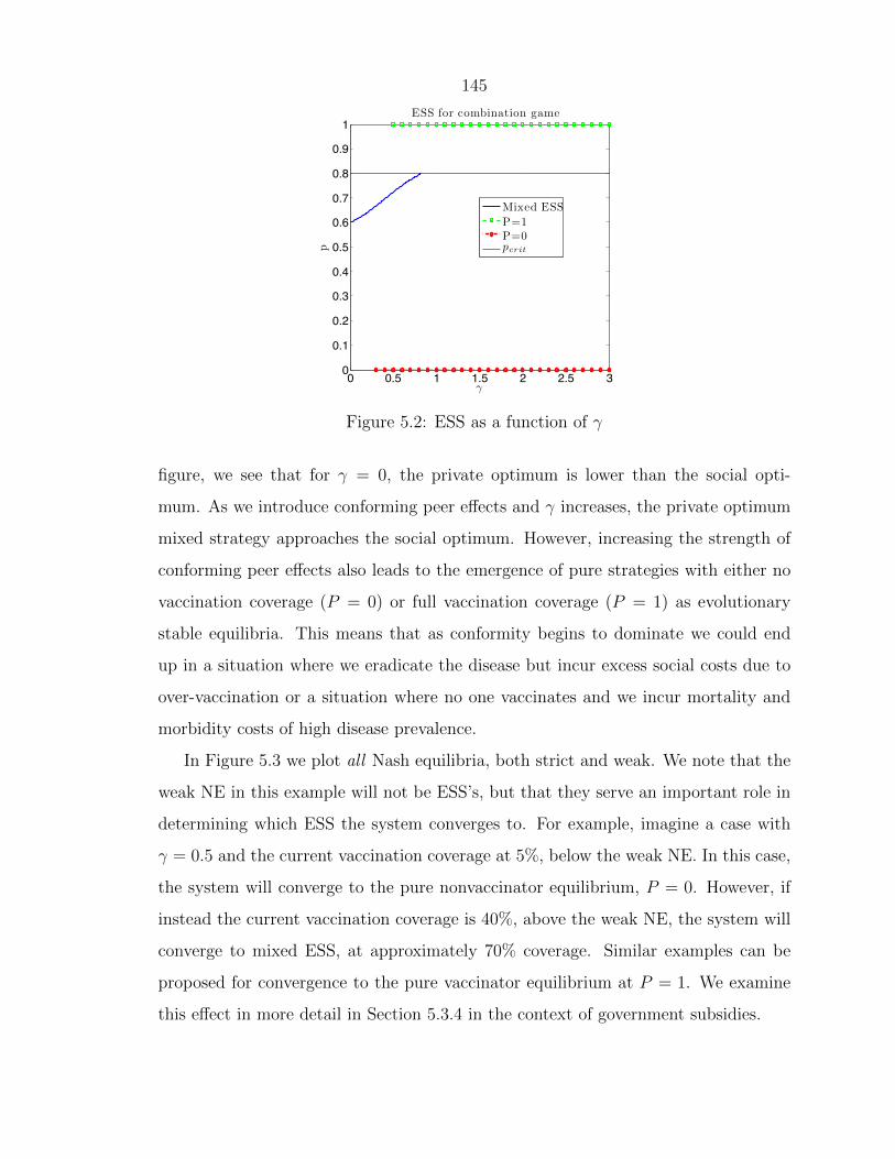
145

0 0.5 1 1.5 2 2.5 30

0.1

0.2

0.3

0.4

0.5

0.6

0.7

0.8

0.9

1

γ

p

ESS for combination game

Mixed ESSP=1P=0pcrit

Figure 5.2: ESS as a function of γ

figure, we see that for γ = 0, the private optimum is lower than the social opti-

mum. As we introduce conforming peer effects and γ increases, the private optimum

mixed strategy approaches the social optimum. However, increasing the strength of

conforming peer effects also leads to the emergence of pure strategies with either no

vaccination coverage (P = 0) or full vaccination coverage (P = 1) as evolutionary

stable equilibria. This means that as conformity begins to dominate we could end

up in a situation where we eradicate the disease but incur excess social costs due to

over-vaccination or a situation where no one vaccinates and we incur mortality and

morbidity costs of high disease prevalence.

In Figure 5.3 we plot all Nash equilibria, both strict and weak. We note that the

weak NE in this example will not be ESS’s, but that they serve an important role in

determining which ESS the system converges to. For example, imagine a case with

γ = 0.5 and the current vaccination coverage at 5%, below the weak NE. In this case,

the system will converge to the pure nonvaccinator equilibrium, P = 0. However, if

instead the current vaccination coverage is 40%, above the weak NE, the system will

converge to mixed ESS, at approximately 70% coverage. Similar examples can be

proposed for convergence to the pure vaccinator equilibrium at P = 1. We examine

this effect in more detail in Section 5.3.4 in the context of government subsidies.

146

0 0.5 1 1.5 2 2.5 30

0.1

0.2

0.3

0.4

0.5

0.6

0.7

0.8

0.9

1

γ

p

NE (weak and strict) for combination game

Mixed ESSP=1P=0pcrit

Weak NEWeak NE

Figure 5.3: All NE as a function of γ

In summary, the game with only nonconforming peer effects, as described in Sec-

tion 5.2, has only one unique evolutionarily stable strategy, either a mixed strategy

below the social optimum, or the pure strategy with no vaccination coverage. In

contrast, the game with both nonconforming and conforming peer effects has a much

richer set of equilibria, admitting up to 3 evolutionarily stable strategies including

a mixed strategy equilibrium and two pure strategy equilibria with either full or no

vaccination coverage. The likelihood of observing pure strategy equilibria with full

vaccination coverage increases with the strength of conforming peer effects and de-

creases with the relative cost of the vaccine. Similarly, the likelihood of observing

pure strategy equilibria with no vaccination coverage increases with the strength of

conforming peer effects and increases with the relative cost of the vaccine.

5.3.3 Social welfare and individually optimal strategies

For the game with both conforming and nonconforming peer effects, we consider

the same social welfare as in Section 5.2, ignoring the additional utility given by the

conformity functions. In other words, we assume that the value derived by individuals

in conforming to a particular strategy does not have any social value. In theory, it is

unclear whether the social value of utility derived from conforming is zero. We make

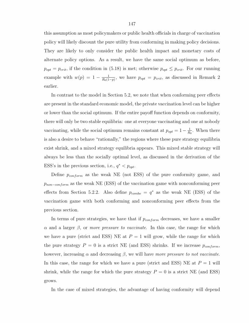
147

this assumption as most policymakers or public health officials in charge of vaccination

policy will likely discount the pure utility from conforming in making policy decisions.

They are likely to only consider the public health impact and monetary costs of

alternate policy options. As a result, we have the same social optimum as before,

popt = pcrit, if the condition in (5.18) is met; otherwise popt ≤ pcrit. For our running

example with w(p) = 1 − 1R0(1−p) , we have popt = pcrit, as discussed in Remark 2

earlier.

In contrast to the model in Section 5.2, we note that when conforming peer effects

are present in the standard economic model, the private vaccination level can be higher

or lower than the social optimum. If the entire payoff function depends on conformity,

there will only be two stable equilibria: one at everyone vaccinating and one at nobody

vaccinating, while the social optimum remains constant at popt = 1− 1R0. When there

is also a desire to behave “rationally,” the regions where these pure strategy equilibria

exist shrink, and a mixed strategy equilibria appears. This mixed stable strategy will

always be less than the socially optimal level, as discussed in the derivation of the

ESS’s in the previous section, i.e., q∗ < popt.

Define pconform as the weak NE (not ESS) of the pure conformity game, and

pnon−conform as the weak NE (ESS) of the vaccination game with nonconforming peer

effects from Section 5.2.2. Also define pcombo = q∗ as the weak NE (ESS) of the

vaccination game with both conforming and nonconforming peer effects from the

previous section.

In terms of pure strategies, we have that if pconform decreases, we have a smaller

α and a larger β, or more pressure to vaccinate. In this case, the range for which

we have a pure (strict and ESS) NE at P = 1 will grow, while the range for which

the pure strategy P = 0 is a strict NE (and ESS) shrinks. If we increase pconform,

however, increasing α and decreasing β, we will have more pressure to not vaccinate.

In this case, the range for which we have a pure (strict and ESS) NE at P = 1 will

shrink, while the range for which the pure strategy P = 0 is a strict NE (and ESS)

grows.

In the case of mixed strategies, the advantage of having conformity will depend

148

on the relative values of pnon−conform and pconform. We state the formal conditions for

conformity to provide an advantage in the theorem below.

Theorem 5.6. The Evolutionarily Stable Strategy (if it exists) of the vaccination

game with both conforming and nonconforming peer effects will be higher than that

of the game with only nonconforming peer effects if and only if the mixed strict Nash

Equilibrium of the vaccination game with nonconforming peer effects is higher than

the mixed weak Nash Equilibrium of the pure conformity game, i.e.,

pnon−conform > pconform ⇐⇒ pcombo > pnon−conform.

Proof. For simplicity, let pnon−conform = pnc and pconform = pc.

pnc > pc (5.80)

⇐⇒ γ�h(pnc) < γ�h(pc) (5.81)

⇐⇒ γ�h(pnc) < 0 (5.82)

⇐⇒ γ�h(pnc)− [diw(pnc)− θm− dv] < [γ�h(pcombo)− diw(pcombo) + θm+ dv]

(5.83)

⇐⇒ γh(pnc)− w(pnc) + r < γh(pcombo)− w(pcombo) + r (5.84)

⇐⇒ pnc < pcombo (5.85)

Line (5.81) come from the fact that h(p) is decreasing in p; line (5.82) since h(pc) = 0;

and lines (5.83) and (5.84) use the equilibrium solutions of the vaccination games.

The last line follows from the fact that, when pcombo exists, γh(p) − w(p) increases

with p, according to mixed strategy ESS condition.

We can see that under certain conditions, the private optimum achieved in the

game with both conforming and nonconforming peer effects will be higher than that

of the game with only nonconforming peer effects; i.e., under certain conditions,

conformity “helps”, bringing the private optimum closer to the socially optimal level.

We illustrate this effect with our running example in Figure 5.4, plotting the ESS’s as

149

a function of r, for various γ and R0. The solid horizontal black line plots the coverage

required for disease eradication (popt = 1 − 1R0), while the black curved dashed line

represents the mixed equilibrium strategy for the game with only nonconforming peer

effects (Section 5.2).

0 0.2 0.4 0.6 0.8 10

0.2

0.4

0.6

0.8

1

r

p

ESS for combination game, R0 = 4, γ = 0.5

Mixed ESSP=1P=0pcr itpnon−conform

(a) pcombo > pnon−conform

0 0.2 0.4 0.6 0.8 10

0.2

0.4

0.6

0.8

1

r

p

ESS for combination game, R0 = 2, γ = 0.2

Mixed ESSP=1P=0pcrit

pnon−conform

(b) pcombo < pnon−conform

Figure 5.4: ESS as a function of r

As r increases, either through an increase of its monetary cost or risk of serious

side effects, the privately optimal strategy will drop below the socially optimal level.

Depending on the disease and cost parameters, the mixed strategy may be higher or

lower than in the game with only nonconforming peer effects — we see both cases

illustrated in Figures 5.4a and 5.4b.

Comparing the mixed strategy ESS with the socially optimal strategy, we see

that pcombo ≤ popt. Exactly how far the individually optimal mixed strategy is from

the social optimum can be easily calculated, as follows. The welfare at the private

optimum, using the social welfare expression from (5.13) is

W (pcombo)

di=

pcombo

di[H + θ(C −m)− dv] +

(1− pcombo)

di[H + θC − diw(pcombo)]

(5.86)

=H + θC

di− w(pcombo) + pcombo(−r + w(pcombo)) (5.87)

=H + θC

di− r − (1− pcombo)γh(pcombo) (5.88)

150

where we have taken advantage of the fact that w(pcombo) = γh(pcombo) + r. Using

this we have the difference between the social welfare at the optimum (using (5.24))

and private ESS as

W (popt)−W (pcombo)

di=

H + θC

di− w(popt) + popt[−r + w(popt)]

− H + θC

di+ r + (1− pcombo)γh(pcombo) (5.89)

= (1− popt)(r − w(popt)) + (1− pcombo)γh(pcombo). (5.90)

In our running example, popt = pcrit, so the difference becomes

W (popt)−W (pcombo)

di= (1− popt)r + (1− pcombo)γh(pcombo). (5.91)

Note that if h(pcombo) > 0, this implies that the difference between the social optimum

and the private optimum will be less than in the game with only nonconforming

peer effects and that pcombo > pnc. In our specific example with linear symmetric

conformity, this holds if pcombo > 1/2.

We note also that the major difference between this game and that with only non-

conforming peer effects is the existence of the pure 100% vaccinator stable strategy.

Lemma 5.4 states the formal conditions for this pure strategy to be stable. In this

case, the classic “free-rider effect” does not hold, and the private optimum is in fact

higher than the social optimum.

5.3.4 Effect of government subsidies

As before, if the government offers subsidies of the monetary cost of the vaccine, indi-

viduals’ expected payoff for vaccinating becomes a function of the subsidy. However,

in contrast to the earlier section, with conforming peer effects present, it will also be

a function of the current coverage:

Evac(p, s) = H + θ(C −m(1− s))− dv + γ�f(p) (5.92)

151

where s represents the percentage of the marginal production cost of the vaccine that

the government is subsidizing. Unlike the game with only nonconforming peer effects,

there is no simple way to write the private optimum as a function of the subsidy, so we

instead focus on general effects and the optimal subsidy in the presence of conforming

peer effects.

In general, when the monetary cost of the vaccine is lowered, the vaccination

coverage will increase, as can be seen by decreasing r and looking at the mixed ESS in

Figure 5.4. When only nonconforming peer effects are present, this produces a counter

effect — as the vaccination coverage goes up, individuals’ incentive to vaccinate goes

down, as their probability of getting infected decreases with the coverage. So, the

advantage gained by lowering the monetary cost of the vaccine is mitigated by the

nonconforming peer effects, and subsides are less effective. However, when conforming

peer effects are present, there is a third effect that can play a role — the individual

desire to vaccinate less as more people vaccinate is balanced by the desire to conform,

resulting in more effective subsidies than when only nonconforming peer effects are

present.

To illustrate these concepts more concretely, we return to our running example,

where f(p) = p, g(p) = 1 − p, and w(p) = 1 − 1R0(1−p) . In this case, the optimal

coverage is pcrit, and in order to achieve this level of vaccination, we solve for the

optimal subsidy. It is easily verified (setting Evac(pcrit, sopt) = Env(pcrit) and solving

for sopt) that

sopt = 1 +dv − γ�

�1− 2

R0

�

θm. (5.93)

Comparing this optimal subsidy to that in Section 5.2.4, we see that if R0 > 2

scombo

opt< snc

opt(5.94)

always — we require less subsidy to achieve the same level of vaccination coverage.

Examining the optimal subsidy further, we look at when conformity “helps” and

when it can “hurt.” In the original game, the optimal subsidy was greater than one

152

— individuals needed to be paid extra, not just have the cost subsidized, in order

to eradicate the disease. When conforming peer effects are present, it is possible to

avoid this problem. To see this, look at the case where sopt ≤ 1. Rearranging and

solving for γ�, we see that this is equivalent to

γ ≥ dv

di�1− 2

R0

� (5.95)

In other words, if the conformity effect is strong enough, individuals do not need to

be paid extra to achieve the social optimum. However, if the conformity effect is too

strong, we might need to impose a “tax” to bring the coverage level down to the social

optimum. Recall that in this combination game, a pure NE and ESS exists at P = 1;

if the conformity is strong enough and a subsidy is used, it is possible that individuals

would choose to always vaccinate. This would certainly lead to disease eradication,

but the extra cost incurred would not make this a socially optimal strategy. Formally,

sopt ≤ 0 if

γ ≥ r

1− 2R0

. (5.96)

In other words, the optimal subsidy will be negative (a tax) if the conforming peer

effects are too strong.

Figure 5.5 plots all Nash equilibrium (weak and strict) of the vaccination game

with conforming and nonconforming peer effects as a function of r. Using this figure,

we can again see the importance of the starting point and the weak NE, as discussed

at the end of Section 5.3.2 in the context of γ. Here, we can see that the subsidy

will also play a role. For example, assume that a new vaccine is being introduced,

and so the starting point is at 0% coverage and suppose r = 0.5. In order to bump

up the coverage to the social optimum, we need to reduce r to approximately r1 =

0.3. However, if we use too large a subsidy and decrease r to r2 = 0.2, the only

equilibrium will be at 100% coverage, incurring too much extra cost. The weak

NE come into play if the starting point is somewhere between 0–100%, as discussed

before. With conforming peer effects, we gain in that the required subsidy to achieve

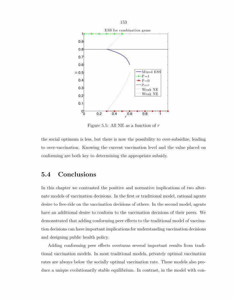
153

0 0.2 0.4 0.6 0.8 10

0.1

0.2

0.3

0.4

0.5

0.6

0.7

0.8

0.9

1

r

p

ESS for combination game

Mixed ESSP=1P=0pcrit

Weak NEWeak NE

Figure 5.5: All NE as a function of r

the social optimum is less, but there is now the possibility to over-subsidize, leading

to over-vaccination. Knowing the current vaccination level and the value placed on

conforming are both key to determining the appropriate subsidy.

5.4 Conclusions

In this chapter we contrasted the positive and normative implications of two alter-

nate models of vaccination decisions. In the first or traditional model, rational agents

desire to free-ride on the vaccination decisions of others. In the second model, agents

have an additional desire to conform to the vaccination decisions of their peers. We

demonstrated that adding conforming peer effects to the traditional model of vaccina-

tion decisions can have important implications for understanding vaccination decisions

and designing public health policy.

Adding conforming peer effects overturns several important results from tradi-

tional vaccination models. In most traditional models, privately optimal vaccination

rates are always below the socially optimal vaccination rate. These models also pro-

duce a unique evolutionarily stable equilibrium. In contrast, in the model with con-

154

forming peer effects, privately optimal vaccination rates can be above or below the

social optimum. In fact, the model produces several evolutionarily stable equilibria

including no vaccination coverage, full vaccination coverage and a mixed strategy

equilibrium. Since this model produces several equilibria vaccination rates, the final

state not only depends on the vaccine and disease parameters but also on the initial

conditions. This means that the effect of changes in the cost of vaccines or new side

effect information might depend on the vaccination rate under the initial equilibrium.

Traditional models also imply that vaccine subsidies are always optimal as private

vaccination rates are always below the social optimum. Given the free-rider problem

these models also imply that even when vaccines are free, coverage required to achieve

disease eradication is impossible. In contrast, in the model with conforming peer

effects, subsidies for vaccination are not always optimal as the privately optimal

vaccination coverage might be above the social optimum. However, in certain cases,

depending on the disease and vaccine parameters, even small subsidies can achieve

disease eradication. In addition, the effects of subsidies can also depend on the initial

conditions.

Overall, these results suggest that conforming peer effects can have important

implications for designing effective public health policy and understanding the effec-

tiveness of interventions for improving vaccination coverage. Yet we know little about

the magnitude of conforming peer effects and the extent to which these peer effects

might vary across diseases, geography, and age group. We also know little about

what factors influence peer effects in vaccination decisions and whether we can design

interventions to change their magnitude. These are all fruitful avenues for future

research.

155

5.5 Appendix: Definitions

Within the vaccination game with nonconforming peer effects, we are interested in

equilibrium strategies to determine the behavior of rational agents. We define a Nash

Equilibrium and an Evolutionarily Stable Strategy (ESS) as given in [62].

Definition 7. A strategy P is a Nash Equilibrium if for all strategies Q �= P

E(Q,P ) ≤ E(P, P ). (5.97)

Note that P is referred to a strict NE if the inequality is strict, or as a weak NE

if the equality holds.

Definition 8. Let ptot = �Q + (1 − �)P represent the total vaccination coverage

when �-fraction of the population deviates from strategy P to Q. A strategy P is an

Evolutionarily Stable Strategy (ESS) if for all Q �= P

E(Q, ptot) < E(P, ptot) (5.98)

holds for all � > 0 sufficiently small.

An alternate definition of an ESS is useful for proving when it exists:

Definition 9. A strategy P is an ESS ⇐⇒ for all strategies Q �= P

(i) E(P, P ) > E(Q,P ), or (5.99)

(ii) E(P, P ) = E(Q,P ) and E(P,Q) > E(Q,Q) (5.100)

Note that the following relations hold for NE and ESS’s:

strict NE =⇒ ESS

ESS =⇒ NE

156

5.6 Appendix: Proofs

In this section we present formal proofs not included in the main body of the chapter.

Proof. (Lemma 5.1) In the context of the vaccination game with only nonconforming

peer effects, the Nash Equilibrium condition from Definition 7 can be rewritten as,

for all Q �= P ,

E(P, P )− E(Q,P ) ≥ 0 (5.101)

⇐⇒ P [Evac] + (1− P )[Env(P )]−Q[Evac]− (1−Q)[Env(P )] ≥ 0 (5.102)

⇐⇒ (P −Q)[Evac − Env(P )] ≥ 0 (5.103)

⇐⇒ (P −Q)[−r + w(P )] ≥ 0. (5.104)

Consider a population following the mixed equilibrium strategy p∗ satisfying w(p∗) =

r. This strategy is clearly a weak NE, since (using the rewritten NE condition from

5.104)

E(p∗, p∗)− E(Q, p∗) = (p∗ −Q)(−r + w(p∗)) = 0. (5.105)

Using Definition 9, p∗ will be an ESS if

E(p∗, Q) > E(Q,Q) ⇐⇒ (p∗ −Q)(−r + w(Q)) > 0. (5.106)

Consider first the case where Q > p∗. In this case, we have p∗ −Q < 0 and

−r + w(Q) < −r + w(p∗) = 0 (5.107)

since by assumption the probability of getting infected w(p) is a strictly decreasing

function with vaccination coverage p (i.e., an individual’s probability of getting in-

fected goes down as more people choose to vaccinate). As a result, (p∗ − Q)(−r +

w(Q)) > 0.

157

Now consider the second case where Q < p∗. In this case, we have p∗−Q > 0 and

−r + w(Q) > −r + w(p∗) = 0 (5.108)

again since the probability of getting infected w(p) is a strictly decreasing function

with vaccination coverage p. Note however that if r > w(0), we have

−r + w(Q) < −w(0) + w(Q) < 0 (5.109)

always. Thus, (p∗ −Q)(−r+w(Q)) > 0 and the mixed equilibrium is an ESS only if

r < w(0), i.e., if the vaccine is sufficiently inexpensive and safe.3

5.7 Appendix: The SIR model with constant pop-

ulation size and vaccination

Using the SIR model with constant population model (birth rate = death rate = µ)

in [13], often used to model childhood diseases, we have,

dS

dt= µ(1− p)− βSI − µS (5.111)

dI

dt= βSI − γI − µI (5.112)

dR

dt= µp+ γI − µR (5.113)

3In the case where r > w(0) (when the relative cost of vaccination to being infected is smallerthan the probability of being infected with zero coverage), there exists a pure strict NE and ESS atP = 0, nobody vaccinating. In this case,

E(P, P )−E(Q,P ) = (P −Q)(Ev(P )−Env(P )) = −Q(Ev(0)−Env(0)) = −Q(−r+w(0)) (5.110)

Thus, E(Q,P ) < E(P, P ) if w(0) < r. If r = 0 (there is no cost or risk associated with thevaccine), any strategy P ≥ pcrit will be a weak NE, including the pure strategy P = 1, everyonevaccinating. However, none of these weak NE will be evolutionarily stable, since they are notresistant to a decrease in vaccination coverage. As a result, everyone will converge to the mixedstrategy p∗ = pcrit.

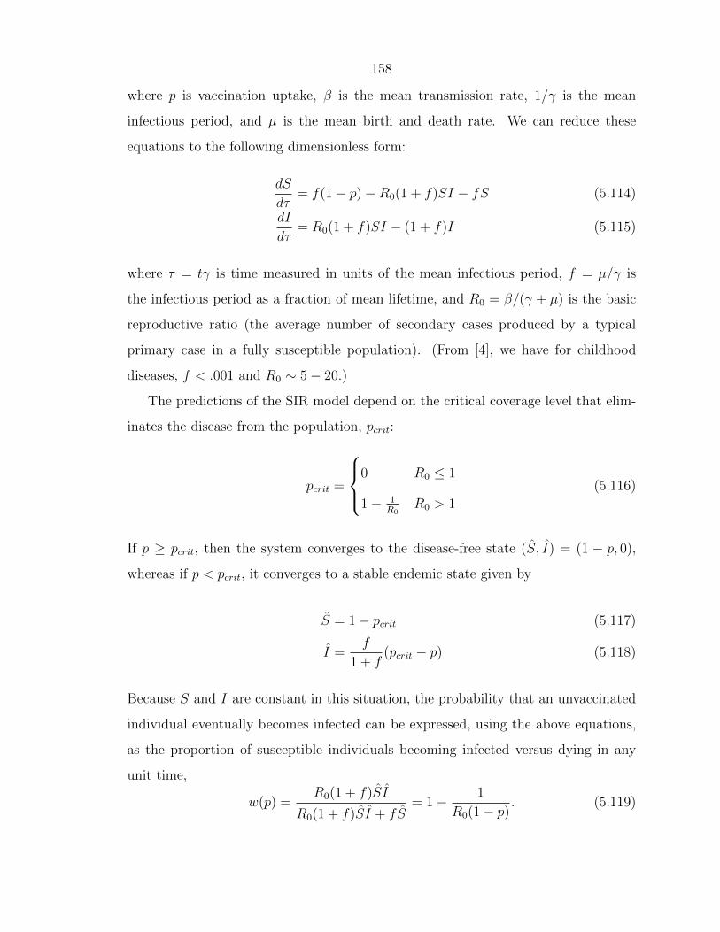
158

where p is vaccination uptake, β is the mean transmission rate, 1/γ is the mean

infectious period, and µ is the mean birth and death rate. We can reduce these

equations to the following dimensionless form:

dS

dτ= f(1− p)−R0(1 + f)SI − fS (5.114)

dI

dτ= R0(1 + f)SI − (1 + f)I (5.115)

where τ = tγ is time measured in units of the mean infectious period, f = µ/γ is

the infectious period as a fraction of mean lifetime, and R0 = β/(γ + µ) is the basic

reproductive ratio (the average number of secondary cases produced by a typical

primary case in a fully susceptible population). (From [4], we have for childhood

diseases, f < .001 and R0 ∼ 5− 20.)

The predictions of the SIR model depend on the critical coverage level that elim-

inates the disease from the population, pcrit:

pcrit =

0 R0 ≤ 1

1− 1R0

R0 > 1(5.116)

If p ≥ pcrit, then the system converges to the disease-free state (S, I) = (1 − p, 0),

whereas if p < pcrit, it converges to a stable endemic state given by

S = 1− pcrit (5.117)

I =f

1 + f(pcrit − p) (5.118)

Because S and I are constant in this situation, the probability that an unvaccinated

individual eventually becomes infected can be expressed, using the above equations,

as the proportion of susceptible individuals becoming infected versus dying in any

unit time,

w(p) =R0(1 + f)SI

R0(1 + f)SI + fS= 1− 1

R0(1− p). (5.119)

159

Thus, we have our infection probability:

w(p) =

1− 1R0(1−p) 0 ≤ p ≤ pcrit

0 pcrit < p ≤ 1(5.120)

Note that w(p) is a decreasing function of p, as shown in Figure 5.6.

0.0 0.2 0.4 0.6 0.8 1.0

0.0

0.2

0.4

0.6

0.8

p (% vaccinated)

w(p

) (Pr

obab

ility

of in

fect

ion)

●●●●●●●●●●●●●●●●●●●●●●●●●●●●●●●●●●●●●●●●●●●●●●●●●●●●●●●●●●●●●●●●●●●●●●●●●

●

●

●

●

●

●

●

●●●●●●●●●●●●●●●●●●●●

Probability of infection

●

R0251020

Figure 5.6: Probability of infection

160

Chapter 6

Conclusion

6.1 Summary of contributions

In this thesis, we have focused on the role of peer effects in social networks, examining

their impact on distributed search, matching markets, epidemic spread, and human

behavior. The goal in each chapter was to leverage these peer effects to reach a deeper

understanding of the problem at hand. For example, in the case of distributed search,

we explored how a distance-dependent probability of connection between peers is re-

quired for a social network to be searchable and developed a novel random network

model: distance-dependent Kronecker graphs. Investigating two very different prob-

lems, matching markets and vaccination decisions, we examined the impact of peer

effects on individual agents’ preferences and decisions. In the context of matching

markets, our focus on peer effects in social networks allowed us to achieve positive

results where most earlier work has only negative results. In our work on epidemics,

we used random social network models to calculate the expected cost of an epidemic

when infection in transmitted between peers (contact-based infection). The common

thread connecting these rather different problems is that each has an underlying social

network; in each case, we asked the question: How might we exploit our knowledge

of peer effects in social networks to use this underlying social network to our advan-

tage? For the remainder of this chapter, we summarize our answer to this question,

restating our major results and describing possible future directions. We conclude

with some general thoughts on the nature of social network research and why it is

161

such an interesting and promising area of investigation.

Distributed Search. In order to determine what makes a social network search-

able by a distributed algorithm using only local information, we used Kleinberg’s idea

of distance-dependent connection probability [75] to generalize a promising random

graph model, Kronecker graphs [81]. Specifically, we developed a mathematically

tractable random network model (distance-dependent Kronecker graphs) incorporat-

ing searchability, where individuals use their local and long-distance connections to

their peers to optimally route a message through the network. This model general-

izes Kronecker graphs, using a family of “distance”-dependent matrices and a new

Kronecker-like operation, as opposed to the static generator matrix used in the origi-

nal Kronecker graph model. As a result, our network model defines both local regular

structures and global distance-dependent connections. While this model is more com-

plicated than the original model, it is more general, as it can generate existing social

network models, and more importantly, networks that are searchable. These prop-

erties emerge naturally from the definition of the embedding of the nodes and the

probability of connection within the family of generator matrices. More generally,

any lattice-based network model with distance-dependent connection probabilities

can be analyzed using the framework described in Chapter 2 for exploring degree dis-

tribution, diameter, and searchability. In particular, our searchability analysis shows

how to make any network model searchable by defining the appropriate probability of

connection. Using this analysis, we are able to show a particularly nice aspect of our

model; i.e., it is rather robust to changes in the long-distance connection probability,

as opposed to earlier models.

Matching Markets with Externalities. Looking at matching markets, we

used a social network to capture the impact of peer effects on individual preferences,

proving that even in the presence of these types of externalities, stable matchings exist

and are achievable by a distributed matching mechanism. Typically, results on this

topic tend to be negative, either proving that stable matchings may not exist, or that

stable matchings are computationally difficult to find. Our goal has been to provide

positive results. To this end, we focused on the case when peer effects are the result

162

of an underlying social network, using utility functions to capture preferences and

examining a new notion of stability, namely, two-sided exchange stability. With this

framework, we proved that a two-sided exchange-stable matching always exists and

that under certain conditions, socially optimal matchings are always stable. Further,

we proved that the impact of the social network structure on the price of anarchy

in such markets happens only through the clustering of the network, which is well

understood for social networks. Interestingly, in our context the price of anarchy has a

dual interpretation as characterizing the degree of inefficiency caused by peer effects.

Our algorithms and efficiency bounds provide a promising approach for designing

optimal matching mechanisms, for the specific housing market considered in Chapter 3

as well as any general market where peer effects change the space of stable matchings.

Epidemic Spread on Complex Networks. Turning to epidemic spread, we

examined the social cost of an epidemic when a disease is spread by social contact,

using tools from random matrix theory to obtain simple solutions highlighting the

importance of the structure of the underlying social network in the final cost of an

epidemic. Using a linearized dynamical system based on the popular SIS model and

a random graph as the underlying network, we calculated the cost of the disease in

the large graph limit and derived bounds for the disease cost for a given graph. This

cost depends on the entire transient behavior of the system and hence this analysis

differs from previous work that usually focuses on the steady-state equilibrium. Our

calculation shows that the disease cost depends on the entire eigen-distribution of

the system matrix, whereas the upper bound depends only on the largest eigenvalue.

Despite its simpler form, the upper bound appears to be tight for some random

graphs, as shown by our simulations. Applying these results to the social cost of an

epidemic (accounting for both the disease cost and the mechanism used to control the

disease), we briefly analyzed the cost of some simple immunization strategies: random

and degree-based one-shot vaccination. We also carefully analyzed the assumptions

made in our linear model and showed graph regimes where our assumptions are valid.

To the best of our knowledge, our approach in Chapter 4 using random matrices is

novel to the study of epidemic processes.

163

Human Behavior in Vaccination Decisions. Motivated by our work in disease

cost, we moved to studying the role of peer effects in vaccination decisions, in order

to explore the impact of (selfish) human behavior in vaccination health policy. We

proposed a game-theoretical model to capture both conforming and nonconforming

peer effects and used this model to determine optimal public health policies regarding

vaccination subsidies. In traditional vaccination decision models with only noncon-

forming peer effects, rational agents desire to free-ride on the vaccination decision of

others. In our model, agents have an additional desire to conform to the vaccination

decisions of their peers. Adding conforming peer effects overturns several important

results from the traditional model. In particular, when only nonconforming peer

effects are present, the privately optimal vaccination rate is a unique evolutionarily

stable strategy and is always below the social optimum. In contrast, when conforming

peer effects are added to the model, privately optimal vaccination rates can be above

or below the social optimum. In fact, the model produces several evolutionary stable

equilibria including no vaccination coverage, full vaccination coverage and a mixed

strategy equilibrium. Since this model produces several equilibria vaccination rates,

the final state not only depends on the vaccine and disease parameters but also on the

initial conditions. In a practical sense this means that the effects of changes in vaccine

cost, or new information on side effects, might depend on the vaccination rate under

the initial equilibrium. The traditional model also implies that vaccine subsidies are

always optimal, since private vaccination rates are always below the social optimum.

Given the free-rider problem, this model also implies that even when vaccines are

free, coverage required to achieve disease eradication is impossible. In contrast, in

our model with nonconforming peer effects, subsidies for vaccination are not always

optimal, since privately optimal vaccination coverage might be above the social opti-

mum. However, in certain cases, depending on disease and vaccine parameters, even

small subsidies can achieve disease eradication. Overall, our results in Chapter 5

suggest that conforming peer effects can have important implications for designing

effective public health policy and understanding the effectiveness of interventions for

improving vaccination coverage.

164

6.2 Future work and applications

The research presented here lays the foundation for further investigation of peer effects

in social networks. Each of the specific topics explored, search, matching markets,

and epidemics, can be extended both theoretically and practically, as described below.

More generally, however, our approach of using network structure and peer effects to

explore problems in diverse areas, from economics to engineering to computer science,

is a promising direction for future social network research. In any problem where

there is an underlying network or process operating on a network, understanding the

structure of that network will be key, and our research provides a useful approach for

tackling these sorts of problems.

Search. While our work in Chapter 2 gives a near complete description of the

characteristics of “distance”-dependent Kronecker graphs, there are many interesting

questions that remain. These include how to parameterize the model from real-world

data sets, and how to incorporate network dynamics. Ideally, given any data set, i.e.,

any collection of related real-world social networks, we would like to be able to find an

appropriate family of distance-dependent matrices to match any desired characteris-

tic of the data set. First, we will need to determine the appropriate embedding of the

network (yielding the first few generator matrices and the “distance” measure) and

then the long-distance probability of connection (giving the rule for the rest of the

generator matrices). Possible approaches include exploring current methods for em-

bedding networks in Euclidean and hyperbolic spaces, but much work still remains to

determine how exactly to separate out and learn the embedding and the long-distance

probability of connection from a real-world social network. Additionally, while the

current model incorporates some measure of growth, growing from a small initiator

matrix to a final n×n adjacency matrix, we would like to better incorporate mobility

into the model so that it is not just a static description of the network at one point

in time. Ideally, our model of growth should mimic the way real social networks grow

and evolve with time, something the current distance-dependent Kronecker graph

model does not capture.

165

Matching Markets. Our current results in Chapter 3 represent only a starting

point for research into the interaction of social networks and many-to-one matchings.

There are a number of simplifying assumptions in this work which would be interesting

to relax. For example, the efficiency bounds we have proven consider only a one-

sided market, where houses do not have preferences over students, students rate

houses similarly, and quotas are exactly met. These assumptions are key to providing

simpler bounds, and they certainly are valid in some matching markets; however

relaxing these assumptions would broaden the applicability of the work greatly.

There are numerous examples of many-to-one matching markets where our re-

sults can provide insight; one of particular interest to us is the matching of incoming

undergraduates to residential houses which happens yearly at Caltech and other uni-

versities. Currently incoming students only report a preference order for houses, and

so are incentivized to collude with friends and not reveal their true preferences. For

such settings, our results highlight the importance of having students report not only

their preference order on houses, but also a list of friends with whom they would like

to be matched. In particular, our simulations clearly show an improvement in social

welfare by considering the social network in the matching mechanism, even with the

very simple mechanisms we examine. Extending this work, we would like to explore

more sophisticated matching mechanisms, perhaps determining the impact of peer

effects on mechanism design (i.e., incentive compatibility and complexity).

Other markets where our approach could prove beneficial include team formation

problems, resource allocation, and on-line ad auctions. When forming teams, whether

in industry or academia, it is important to consider the makeup of the team (diverse

skills and backgrounds) as well as the ability of team members to work together. Our

model can easily be extended to this scenario, using a weighted social network to

capture team members’ affinity for each other and our utility functions to capture

complementarities. In terms of on-line ad auctions, we would like to use our model

to explore the impact of ad placement on effectiveness — examining the impact of

neighboring competing or complementary ads on click-through rate. If neighboring

ads do have a positive and/or negative impact, we could use our model to design ad

166

auctions that take this effect into account. In general, we should be able to extend our

results to any sort of market where peer effects change the space of stable matchings.

Epidemics. To extend the work on epidemics on complex networks, we would

like to investigate both theoretical and practical refinements of our model. We can

consider more sophisticated epidemic models (SIR, etc.) as well as immunization

based on the strategic behavior of agents. Moreover, a case study with real data from

communicable diseases like influenza or herpes would provide more insight into the

accuracy and predictive power of these models in real-world scenarios, as well as help

refine the per node cost of disease which we have assumed is a single parameter. In

general, our random network approach is a promising direction to tackle the problem

of epidemic spread on network — our simulations show that at least under certain

infection and graph parameters, our results are fairly accurate, giving us hope to

quantify the cost of an epidemic on real-world networks. The approach and the

random matrix tools we use are fairly general; we hope to extend the tools, techniques

and ideas in our results to further study complex processes on complex networks.

For example, we can combine our work on epidemics and vaccination decisions to

investigate dynamic vaccination games on networks, where individuals make vaccina-

tion decisions at each point in time, based on their local information about the current

epidemic state and perhaps influenced by their peers to make particular choices. This

is a very interesting and challenging theoretical problem to pursue, but unfortunately,

we know little about real-world peer effects. Practically, we know little about the mag-

nitude of conforming peer effects and the extent to which these peer effects might vary

across diseases, geography, and age group, what factors influence peer effects in vacci-

nation decisions and whether we can design interventions to change their magnitude.

Quantifying real-world peer effects is a fruitful avenue for future research, perhaps

requiring some sort of real-world data gathering and study. On the theoretical side,

this general approach can also be applied to other problems such as technology adop-

tion, dynamic patching of viruses on computer networks, and others — any problem

where individual agents make decisions based on information available through their

peers and perhaps can be influenced by conforming peer effects.

167

6.3 Concluding thoughts

Social network research requires translation between the fields of engineering, com-

puter science, economics, public policy and sociology. Often, the challenge can be

simply to find a common language; a thorough literature search on a given topic

may require multiple searches across disciplines using different keywords. As with

all interdisciplinary research, in order to not reinvent the wheel, one must be careful

to examine the research in each area to determine where novel contribution can be

made. Despite the challenges, the potential benefit of such research is huge. Lever-

aging knowledge from one area not only allows us to reach deeper insights about

problems in a different one, but also can influence the questions we ask and the

research problems we decide to study. For example, existing research in sociology

on real-world data sets may point to an underlying phenomenon. This knowledge

provides the motivation for computer scientists and statistical physicists to propose

and study various random network models explaining the origin of said phenomenon.

Closing the loop, real-world studies can then be used to validate these random net-

work models, determining which model is most appropriate for studying a particular

topic. Economists can then apply such models to studying economic interactions in

networked markets, while engineers can use the same models to design protocols and

algorithms to facilitate such markets. This is just one rather general example where

this type of interdisciplinary research provides a large reward — many more specific

examples exist, including the work presented here.

In many cases, the results in one area lead to questions in another. For example,

in our attempt to define a mathematically tractable searchable network model, we

discovered a tension between searchability and a heavy-tailed degree distribution.

Our results state that at least in the case of lattice-based network models, the two

characteristics are incompatible. Yet, both have been observed in social networks.

This apparent contradiction points to the need for more careful investigation using

real-world and on-line data sets, determining the exact circumstances under which

both characteristics exist, and hopefully determining an improvement to the model

168

to make it more realistic. In another example, we found that while our matching

mechanisms incorporating social network knowledge yield a better match than the

existing one for the Caltech housing market, the improvement is not drastic. The

existing match of students to houses already does a pretty good job of matching friends

together. At first glance, this is a negative result, but upon further investigation, it is

pointing to a deeper issue: causation and network formation. The current data set we

use includes all undergraduate students, freshman through senior. Seniors have been

living in their respective houses for four years and likely have formed many friendships

within their houses. Thus, the network is already rather well clustered into the

various houses, and while our matching mechanisms do provide some improvement,

this increase in social welfare is not as much as would be expected compared to

starting at a purely random match. This rather simple observation leads to more

questions involving network formation, and further avenues of investigation. Perhaps

we can use our data set, differentiating between each class of students, to determine

the effect of housing assignment on the social network and vice versa.

In conclusion, using the interdisciplinary knowledge required for social network

research can help us understand our role in an increasingly (social-)networked world,

as well as design better solutions to the problems our networked world poses.

169

Bibliography

[1] R. Albert and A. Barabasi. Statistical mechanics of complex networks. Reviews

of Modern Physics, 74, 2002.

[2] J. Alcalde. Exchange-proofness or divorce-proofness? Stability in one-sided

matching markets. Review of Economic Design, 1:275–287, 1994.

[3] G.W. Anderson, A. Guionnet, and O. Zeitouni. An Introduction to Random Ma-

trices, volume 118 of Cambridge Studies in Advanced Mathematics. Cambridge

University Press, 2010.

[4] R.M. Anderson and R.M. May. Infectious Diseases of Humans. Oxford Univer-

sity Press, 1991.

[5] M. Angeles Serrano, D. Krioukov, and M. Boguna. Self-similarity of complex

networks and hidden metric spaces. Physics Review Letters, 100, 2008.

[6] E. Anshelevich, S. Das, and Y. Naamad. Anarchy, stability, and utopia: Cre-

ating better matchings. In SAGT ’09, pages 159–170, 2009.

[7] H. Aziz, F. Brandt, and H.G. Seedig. Stable partitions in additively separable

hedonic games. Computing Research Repository, 2010.

[8] M. Baccara, A. Imrohoroglu, A. Wilson, and L. Yariv. A field study on matching

with network externalities. The American Economic Review, 102, 2012.

[9] P. Bajari and J. Fox. Measuring the efficiency of an FCC spectrum auction.

Working Paper 11671, National Bureau of Economic Research, 2009.

170

[10] P. Bak, K. Chen, and C. Tang. A forest-fire model and some thoughts on

turbulence. Phys. Lett. A, 147:297300, 1990.

[11] A. Barabasi and R. Albert. Emergence of scaling in random networks. Science,

286:509–512, 1999.

[12] M. Barthelemy, A. Barrat, R. Pastor-Satorras, and A. Vespignani. Velocity and

Hierarchical Spread of Epidemic Outbreaks in Scale-Free Networks. Phys. Rev.

Lett., 92(17), 2004.

[13] C.T. Bauch. Vaccination and the theory of games. Proceedings of The National

Academy of Sciences, 101:13391–13394, 2004.

[14] C.T. Bauch. Imitation dynamics predict vaccinating behavior. Proceedings of

the Royal Society B: Biological Sciences, 272(1573):1669–1675, 2005.

[15] C.T. Bauch, A.P. Galvani, and D.J. Earn. Group interest versus self-interest in

smallpox vaccination policy. Proceedings of the National Academy of Sciences,

100(18):10564–10567, 2003.

[16] E. Bodine, B. Hassibi, and A. Weirman. Generalizing Kronecker graphs in

order to model searchable networks. In Proc. Forty-Seventh Annual Allerton

Conference, 2009.

[17] E. Bodine-Baron, S. Bose, B. Hassibi, and A. Wierman. Minimizing the social

cost of an epidemic. LNICST, Proc. GameNets 2011, 2011.

[18] E. Bodine-Baron, B. Hassibi, and A. Wierman. Distance-dependent Kronecker

graphs for modeling social networks. IEEE Journal of Selected Topics in Signal

Processing, 4(4):718–731, Aug. 2010.

[19] E. Bodine-Baron, C. Lee, A. Chong, B. Hassibi, and A. Wierman. Peer effects

and stability in matching markets. In Giuseppe Persiano, editor, Algorithmic

Game Theory, volume 6982 of Lecture Notes in Computer Science, pages 117–

129. Springer Berlin/Heidelberg, 2011.

171

[20] E. Bodine-Baron, S. Nowak, N. Sood, and R. Vardavas. Conforming and non-

conforming peer effects in vaccination decisions. Working paper, 2012.

[21] A. Bogomolnaia and M. Jackson. The stability of hedonic coalition structures.

Games and Economic Behavior, 38(2):201–230, 2002.

[22] M. Boguna and D. Krioukov. Navigating ultrasmall worlds in ultrashort time.

Physical Review Letters, 102:058701, 2009.

[23] M. Boguna, D. Krioukov, and kc claffy. Navigability of complex networks.

Nature Physics, 5:74–80, 2009.

[24] M. Boguna, R. Pastor-Satorras, and A. Vespignani. Absence of Epidemic

Threshold in Scale-Free Networks with Degree Correlations. Phys. Rev. Lett.,

90(2), 2003.

[25] B. Bollobas. Random Graphs. Academic Press, Inc., 1985.

[26] S. Bose, E. Bodine-Baron, B. Hassibi, and A. Wierman. Cost of epidemic spread

on complex networks: A random matrix approach. Working paper, 2012.

[27] L. Bownds, R. Lindekugel, and P. Stepak. Economic impact of a Hepatitis A

epidemic in a mid-sized urban community: The case of Spokane, Washington.

Journal of Community Health, 38(4), 2003.

[28] S. Branzei and K. Larson. Coalitional affinity games and the stability gap. In

Proc. 21st Intl. Joint Conf. on Artificial Intelligence (IJCAI), pages 1319–1320,

2009.

[29] N. Burani and W.S. Zwicker. Coalition formation games with separable prefer-

ences. Mathematical Social Sciences, 45:27–52, 2003.

[30] K. Cechlarova and D. Manlove. On the complexity of exchange-stable room-

mates. Discrete Applied Mathematics, 116(3):279–287, 2002.

172

[31] K. Cechlarova and D. Manlove. The exchange-stable marriage problem. Discrete

Applied Mathematics, 152(1–3):109–122, 2005.

[32] M. Cha, A. Mislove, and K.P. Gummadi. A measurement-driven analysis of

information propagation in the flickr social network. Proc. 18th WWW Conf.,

pages 721–730, 2009.

[33] D. Chakrabarti, Y. Wang, C. Wang, J. Leskovec, and C. Faloutsos. Epidemic

thresholds in real networks. ACM Trans. on Info. and System Security (TIS-

SEC), 10(4), 2008.

[34] H. Chen, H. Jin, J. Sun, and Z. Han. Efficient immunization algorithm for

peer-to-peer networks. Lec. Notes in Comp. Sci., 3296:143–178, 2005.

[35] F. Chung and L. Lu. Complex Graphs and Networks. AMS, 2006.

[36] S. Clark, A. Cowan, and P. Wortley. Influenza vaccination attitudes and prac-

tices among US registered nurses. American Journal of Infection Control,

37(7):551–556, 2009.

[37] R. Cohen, S. Havlin, and D. ben Avraham. Efficient immunization strategies

for computer networks and populations. Phys. Rev. Lett., 91(24), 2003.

[38] A. Cvetkovski and M. Crovella. Hyperbolic embedding and routing for dynamic

graphs. In Proc. of Infocom, 2009.

[39] D. Daley and J. Gani. Epidemic Modeling: An Introduction. Cambridge Uni-

versity Press, 2005.

[40] A. Datar, A. Mukherji, and N. Sood. Health infrastructure and immunization

coverage in rural India. Indian Journal of Medicine, 125:31–42, January 2007.

[41] Wikipedia vote data set: Stanford large network dataset collection. http:

//snap.stanford.edu/data/wiki-Vote.html.

173

[42] J.H. Dreze and J. Greenberg. Hedonic coalitions: Optimality and stability.

Econometrica, 48(4):987–1003, 1980.

[43] B. Dutta and J. Masso. Stability of matchings when individuals have preferences

over colleagues. Journal of Economic Theory, 75(2):464–475, 1997.

[44] F. Echenique and M. Yenmez. A solution to matching with preferences over

colleagues. Games and Economic Behavior, 59(1):46–71, 2007.

[45] A. Edelman and N.R. Rao. Random matrix theory. Acta Numerica, 14:233–297,

2005.

[46] E. Elkind and M. Wooldridge. Hedonic coalition nets. In Proc. 8th Intl. Joint

Conf. on Autonomous Agents and Multi-Agent Systems (AAMAS), pages 417–

424, 2009.

[47] J. Ensminger. The Caltech Project, 2010. Unpublished dataset.

[48] W. Evans, W. Oates, and R. Schwab. Measuring peer group effects: A study

of teenage behavior. Journal of Political Economy, 100(5):966–91, 1992.

[49] F. Fenner. Smallpox and Its Eradication (History of International Public

Health), No. 6. Geneva: World Health Organization, 1988.

[50] J. Fox. Estimating matching games with transfers. Working Paper 14382,

National Bureau of Economic Research, October 2008.

[51] L. Freeman. The Development of Social Network Analysis. Empirical Press,

2006.

[52] F. Fu, D. Rosenbloom, L. Wang, and M. Nowak. Imitation dynamics of vacci-

nation behavior on social networks. Proceedings of the Royal Society Biological

Sciences, 2010.

[53] M. Gairing and R. Savani. Computing stable outcomes in hedonic games. In

Proc. 3rd Intl. Sym. on Algorithmic Game Theory (SAGT), 2010.

174

[54] D. Gale and L.S. Shapley. College admissions and the stability of marriage.

The American Mathematical Monthly, 69(1):9–15, January 1962.

[55] A. Gaviria and S. Raphael. School-based peer effects and juvenile behavior.

The Review of Economics and Statistics, 83(2):257–268, 2001.

[56] M. S. Granovetter. The strength of weak ties. The American Journal of Soci-

ology, 78(6):13601380, 1973.

[57] Q. Gu and N. Sood. Do people taking flu vaccines need them the most? PLoS

ONE, 6(12), 12 2011.

[58] I.E. Hafalir. Stability of marriage with externalities. International Journal of

Game Theory, 37:353–370, 2008.

[59] O. Haggstrom. Finite Markov Chains and Algorithmic Applications. Cambridge

University Press, 2001.

[60] B. Hanratty, T. Holt, E. Duffell, W. Patterson, M. Ramsay, J.M. White, L. Jin,

and P. Litton. UK measles outbreak in non-immune anthroposophic communi-

ties: the implications for the elimination of measles from Europe. Epidemiology

and Infection, 125:377–383, 2000.

[61] L. Henderson, C. Millett, and N. Thorogood. Perceptions of childhood immu-

nizations in a minority community: qualitative study. Journal of the Royal

Society of Medicine, 101(5):244–251, 2008.

[62] J. Hofbauer and K. Sigmund. Evolutionary Games and Population Dynamics.

Cambridge University Press, 1998.

[63] P. W. Holland and S. Leinhardt. Transitivity in structural models of small

groups. Comparative Group Studies, 2:107–124, 1971.

[64] R.A. Horn and C.R. Johnson. Matrix Analysis. Cambridge University Press,

2005.

175

[65] L. Huang, K. Park, and Y. C. Lai. Information propagation on modular net-

works. Phys. Rev. E, 73(3), Mar 2006.

[66] R. Irving. Stable matching problems with exchange restrictions. Journal of

Combinatorial Optimization, 16:344–360, 2008.

[67] M. Jackson. Social and Economic Networks. Princeton University Press, 2008.

[68] P. Jacquet, B. Mans, and G. Rodolakis. Information propagation speed in

mobile and delay tolerant networks. IEEE Trans. on Info. Theory, 56(10):5001

–5015, 2010.

[69] D. Johnson, K. Nichol, and K. Lipczynski. Barriers to adult immunization. The

American Journal of Medicine, 121(7, Supplement 2):S28–S35, 2008.

[70] R. Kannan, S. Vempala, and A. Vetta. On clusterings: Good, bad and spectral.

Journal of the ACM, 51(3):497–515, 2004.

[71] E. Kenah and James M. Robins. Second look at the spread of epidemics on

networks. Physical Review E (Statistical, Nonlinear, and Soft Matter Physics),

76:036113, 2007.

[72] W.O. Kermack and A.G. McKendrick. A contribution to the mathematical

theory of epidemics. Proc. Roy. Soc. Lond. A, 115:700–721, 1927.

[73] B. Klaus and F. Klijn. Stable matchings and preferences of couples. Journal of

Economic Theory, 121:75–106, 2005.

[74] B. Klaus and F. Klijn. Paths to stability for matching markets with couples.

Games and Economic Behavior, 58:154–171, 2007.

[75] J. Kleinberg. The small-world phenomenon: An algorithmic perspective. In

Proc. of the 32nd ACM Symposium on Theory of Computing, pages 163–170,

2000.

176

[76] J. Kleinberg. Complex networks and decentralized search algorithms. In Proc.

of International Conference of Mathematicians, 2006.

[77] F. Kojima and P. Pathak. Incentives and stability in large two-sided matching

markets. American Economic Review, 99(3):608–627, 2009.

[78] D. Krioukov, F. Papadopoulos, M. Boguna, and A. Vahdat. Greedy forwarding

in scale-free networks embedded in hyperbolic metric spaces. In Proc. of MAMA

Workshop at Sigmetrics, 2009.

[79] D. Krioukov, F. Papadopoulos, A. Vahdat, and M. Boguna. Curvature and

temperature of complex networks. Physical Review E, 80:635101, 2009.

[80] J. Leskovec. Dynamics of Large Networks. PhD thesis in Computer Science,

Carnegie Mellon University, 2008.

[81] J. Leskovec, D. Chakrabarti, J. Kleinberg, and C. Faloutsos. Realistic, mathe-

matically tractable graph generation and evolution, using Kronecker multiplica-

tion. In Conf. on Principles and Practice of Knowledge Discovery in Databases,

2005.

[82] J. Leskovec, J. Kleinberg, and C. Faloutsos. Graphs over time: densification

laws, shrinking diameters and possible explanations. In Proc. of ACM SIGKDD

Conf. on Knowledge Discovery in Data Mining, pages 177–187, 2005.

[83] J. Logan. Disparities in influenza immunization among US adults. Journal of

the National Medical Association, 101(2):161–166, 2009.

[84] P. Lundborg. Having the wrong friends? Peer effects in adolescent substance

use. Journal of Health Economics, 25, 2006.

[85] M. Mahdian and Y. Xu. Stochastic Kronecker graphs. In In WAW07: Proc.

of Workshop On Algorithms And Models For The Web-Graph, pages 179–186,

2007.

177

[86] C. Martel and V. Nguyen. Analyzing Kleinberg’s and other small-world mod-

els. In In PODC ’04: Proc. of ACM Symposium on Principles of Distributed

Computing, pages 179–188, 2004.

[87] T. May and R. Silverman. Clustering of exemptions as a collective action threat

to herd immunity. Vaccine, 21(11–12):1048–1051, 2003.

[88] M. McPherson, L. Smith-Lovin, and J. Cook. Birds of a feather: Homophily in

social networks. Annual Review of Sociology, 27:414–444, 2001.

[89] S. Milgram. The small-world problem. Psychology Today, 2:60, 1967.

[90] J. Miller and J. Hyman. Effective vaccination strategies for realistic social

networks. Physica A: Statistical Mechanics and its Applications, 386(2):780–

785, 2007.

[91] C. Moore and M.E.J. Newman. Epidemics and percolation in small-world net-

works. Physical Review E, 61(5):5678, 2000.

[92] M.E.J. Newman. Spread of epidemic disease on networks. Physical Review E,

66(1):016128, 2002.

[93] M.E.J. Newman. The structure and function of complex networks. SIAM

Review, 2003.

[94] M.E.J. Newman. Random graphs as models of networks. In Handbook of Graphs

and Networks, pages 35–68. Wiley-VCH, 2005.

[95] M. Olsen. Nash stability in additively separable hedonic games and community

structures. Theory Comput Sys., 45:917–925, 2009.

[96] F.W. O’Reilly, G.W. Cran, and A.B. Stevens. Factors affecting influenza vaccine

uptake among health care workers. Occupational Medicine, 55(6):474–479, 2005.

[97] P. Erdos and A. Renyi. On random graphs. Publicationes Mathematicae 6, page

290297, 1959.

178

[98] M. Ostrovsky. Stability in supply chain networks. The American Economic

Review, 98(3):897–923, 2008.

[99] A. Parker, W. Staggs, G. Dayan, I. Ortega-Sanchez, P. Rota, L. Lowe, P. Board-

man, R. Teclaw, C. Graves, and C. LeBaron. Implications of a 2005 measles

outbreak in Indiana for sustained elimination of measles in the United States.

New England Journal of Medicine, 355(5):447–455, 2006.

[100] R. Pastor-Satorras and A. Vespignani. Epidemic Spreading in Scale-Free Net-

works. Phys. Rev. Lett., 86:3200–3203, 2001.

[101] R. Pastor-Satorras and A. Vespignani. Epidemic dynamics in finite size scale-

free networks. Phys. Rev. E, 65, 2002.

[102] R. Pastor-Satorras and A. Vespignani. Immunization of complex networks.

Phys. Rev. E, 65, 2002.

[103] C. Peng, X. Jin, and M. Shi. Epidemic threshold and immunization on

generalized networks. Physica A: Statistical Mechanics and its Applications,

389(3):549–560, 2010.

[104] J. Phelps, R. Lewis, L. Mobilio, D. Perry, and N. Raman. Viral marketing

or electronic word-of-mouth advertising: Examining consumer responses and

motivations to pass along email. Journal of Advertising Research, 44, 2004.

[105] T. Philipson. Economic epidemiology and infectious diseases. In A. J. Cu-

lyer and J. P. Newhouse, editors, Handbook of Health Economics, volume 1 of

Handbook of Health Economics, chapter 33, pages 1761–1799. Elsevier, 2000.

[106] M. Pycia. Stability and preference alignment in matching and coalition forma-

tion. Econometrica, 80(1):323–362, 2012.

[107] F. Radicchi, C. Castellano, F. Cecconi, V. Loreto, and D. Parisi. Defining and

identifying communities in networks. Proc. National Academy of Sciences USA,

101(9):2658–2663, 2004.

179

[108] V. Ramasubramanian and D. Malkhi. On the treeness of internet latency and

bandwidth. In Proc. of ACM Sigmetrics, pages 61–72, 2009.

[109] N. Rao, M. Mobius, and T. Rosenblat. Social networks and vaccination deci-

sions. Federal Reserve Bank of Boston Working Papers, 2007.

[110] P. Revilla. Many-to-one matching when colleagues matter. Working paper 146,

Fondazione Eni Enrico Mattei Working Papers, 2007.

[111] M. Richardson and P. Domingos. Mining knowledge-sharing sites for viral mar-

keting. Proc. 8th ACM SIGKDD, pages 61–70, 2002.

[112] E. Ronn. NP-complete stable matching problems. Journal of Algorithms,

11:285–304, 1990.

[113] A.E. Roth. The evolution of the labor market for medical interns and residents:

A case study in game theory. Journal of Political Economics, 92:991–1016,

1984.

[114] A.E. Roth, U.G. Rothblum, and J.H. Vande Vate. Stable matchings, optimal

assignments and linear programming. Mathematics of Operations Research,

18(4):803–828, 1993.

[115] A.E. Roth and M. Sotomayor. Two-sided matching: A study in game-theoretic

modeling and analysis. Cambridge University Press, 1990.

[116] A.E. Roth and J.H. Vande Vate. Random paths to stability in two-sided match-

ing. Econometrica, 58:1475–1480, 1990.

[117] R. Rubin, C. Harrington, A. Poon, K. Dietrich, J. Greene, and A. Moiduddin.

The Economic Impact of Staphylococcus aureus Infection in New York City

Hospitals. Emerging Infectious Diseases, 5(1), 1999.

[118] B. Sacerdote. Peer effects with random assignment: Results for Dartmouth

roommates. Quarterly Journal of Economics, 116:681–704, 2001.

180

[119] T. Santibanez, M. Nowalk, R. Zimmerman, I. Jewell, I. Bardella, S. Wilson,

and M. Terry. Knowledge and beliefs about influenza, pneumococcal disease,

and immunizations among older people. Journal of the American Geriatrics

Society, 50(10):1711–1716, 2002.

[120] H. Sasaki and M. Toda. Two-sided matching problems with externalities. Jour-

nal of Economic Theory, 70(1):93–108, 1996.

[121] D. Schmid, H. Holzmann, S. Abele, S. Kasper, S. Konig, S. Meusburger,

H. Hrabcik, A. Luckner-Hornischer, E. Bechter, A. DeMartin, J. Stirling,

A. Heißenhuber, A. Siedler, H. Bernard, G. Pfaff, D. Schorr, M.S. Ludwig, H.P.

Zimmerman, Ø. Løvoll, P. Aavitsland, and F. Allerberger. An ongoing multi-

state outbreak of measles linked to non-immune anthoposophic communities in

Austria, Germany, and Norway. Eurosurveillance, 13(16):18838, 2008.

[122] J. Scott. Social Network Analysis: A Handbook. Sage, 2nd edition, 2000.

[123] J. Shi and J. Malik. Normalized cuts and image segmentation. IEEE Trans. of

Pattern Analysis and Machine Intelligence, 22(8):888–905, 2000.

[124] B. Stewart-Freedman and N. Kovalsky. An ongoing outbreak of measles linked

to the UK in an ultra-orthodox Jewish community in Israel. Eurosurveillance,

12(38):3270, 2007.

[125] T. Tao. Topics in random matrix theory, volume 132 of Graduate Studies in

Mathematics. American Mathematical Society, 2012.

[126] A.M. Tulino and S. Verdu. Random matrix theory and wireless communications,

volume 1. Now Publishers, Inc., 2004.

[127] G. Van Essen, M. Kuyvenhoven, and R. De Melker. Why do healthy elderly

people fail to comply with influenza vaccination? Age and Ageing, 26(4):275–

279, 1997.

181

[128] P. Van Mieghem. Graph spectra for complex networks. Cambridge University

Press, 2011.

[129] C. Wang, J.C. Knight, and M.C. Elder. On computer viral infection and the

effect of immunization. Proc. ACSAC ’00, pages 246–256, 2000.

[130] Y. Wang, D. Chakrabarti, C. Wang, and C. Faloutsos. Epidemic spreading in

real networks: An eigenvalue viewpoint. Proc. Symp. Reliable Dist. Systems,

2003.

[131] S. Wasserman and K. Faust. Social Network Analysis: Methods and Applica-

tions. Cambridge University Press, 1994.

[132] D. Watts. Six Degrees: The Science of a Connected Age. W. W. Norton and

Company, 2003.

[133] D.J. Watts and S.H. Strogatz. Collective dynamics of small-world networks.

Nature, 393:440, 1998.

[134] C. Winston, P. Wortley, and K. Lees. Factors associated with vaccination of

medicare beneficiaries in five u.s. communities: Results from the racial and

ethnic adult disparities in immunization initiative survey, 2003. Journal of the

American Geriatrics Society, 54(2):303–310, 2006.