Analysis of Traffic Load Effects on Railway Bridges9338/FULLTEXT01.pdf · Analysis of Traffic Load...

Analysis of Traffic Load Effects

on Railway Bridges

Gerard James

Structural Engineering DivisionRoyal Institute of TechnologySE-100 44 Stockholm, Sweden

TRITA-BKN. Bulletin 70, 2003ISSN 1103-4270ISRN KTH/BKN/B--70--SE

Doctoral Thesis

Akademisk avhandling som med tillstand av Kungl Tekniska Hogskolan i Stock-holm framlagges till offentlig granskning for avlaggande av teknologie doktorsexa-men fredagen den 23:a maj kl 10.00 i sal V1, Teknikringen 72, Kungliga TekniskaHogskolan, Valhallavagen 79, Stockholm.

c©Gerard James 2003

Abstract

The work presented in this thesis studies the load and load effects of traffic loads onrailway bridges. The increased knowledge of the traffic loads, simulated using fieldmeasurements of actual trains, are employed in a reliability analysis in an attemptat upgrading existing railway bridges.

The study utilises data from a weigh-in-motion site which records, for each train,the train speed, the loads from each axle and the axle spacings. This data of actualtrain configurations and axle loads are portrayed as moving forces and then used incomputer simulations of trains crossing two dimensional simply supported bridgesat constant speed. Only single track short to medium span bridges are considered inthe thesis. The studied load effect is the moment at mid-span. From the computersimulations the moment history at mid-span is obtained.

The load effects are analysed by two methods, the first is the classical extremevalue theory where the load effect is modelled by the family of distributions calledthe generalised extreme value distribution (GEV). The other method adopts thepeaks-over-threshold method (POT) where the limiting family of distributions forthe heights to peaks-over-threshold is the Generalised Pareto Distribution (GPD).The two models are generally found to be a good representation of the data.

The load effects modelled by either the GEV or the GPD are then incorporated intoa reliability analysis in order to study the possibility of raising allowable axle loadson existing Swedish railway bridges. The results of the reliability analysis show thatthey are sensitive to the estimation of the shape parameter of the GEV or the GPD.

While the study is limited to the case of the ultimate limit state where the effectsof fatigue are not accounted for, the findings show that for the studied cases anincrease in allowable axle load to 25 tonnes would be acceptable even for bridgesbuilt to the standards of 1940 and designed to Load Model A of that standard. Evenan increase to both 27.5 and 30 tonnes appears to be possible for certain cases. It isalso observed that the short span bridges of approximately four metres are the mostsusceptible to a proposed increase in permissible axle load.

Keywords: bridge, rail, traffic load, load effect, dynamic amplification factor, ex-treme value theory, peaks-over-threshold, reliability theory, axle loads, field data.

i

Acknowledgements

The research work presented in this thesis was carried out at the Department ofCivil and Architectural Engineering at the Royal Institute of Technology (KTH) atthe Division of Structural Design and Bridges between 1998 and 2003. This researchwas jointly financed by the Swedish National Rail Administration (Banverket) andthe Royal Institute of Technology. I thank them both for the financial support thatprovided this research opportunity.

I thank my supervisor Professor Hakan Sundquist for his almost boyish enthusiasm,for his encouragement and also for his patience with me. Thanks are also due tomay co-supervisor Dr. Raid Karoumi partly for the use of his computer program andalso for his advice and guidance. I also thank both of them for the proof-reading ofthis thesis and their helpful comments and suggestions.

The research shown here is part of a larger research program, within the StructuralDesign and Bridges Division, designed to investigate the traffic loads and traffic loadeffects on bridges. The group has been interesting and stimulating to work withinand has provided many an interesting discussion. Thanks go to the members of thisgroup who apart from my supervisors also include Dr. Abraham Getachew who hasbecome a good friend.

Thanks are also expressed to Mr. Lennart Askling and Mr. Lennart Andersson ofthe Swedish National Rail Administration. The first for his help with supplyingdocuments and the second for his assistance with the field data.

I also thank Mr. Bjorn Paulsson of the Swedish National Rail Administration forthe opportunity of partaking in a number of conferences within the UIC BridgeCommittee on the dynamics of railway bridges.

A warm thankyou to all the staff at the Department of Civil and ArchitecturalEngineering and the former members of staff at the Department of Structural En-gineering for creating a pleasant working environment and providing much laughterduring coffee breaks. A special mention as regards the last matter goes to Dr. Gun-nar Tibert and Dr. Anders Ansell.

My greatest appreciation, however, is to my loving wife Kristina Oberg and my twolovely children, Emilia and Liam. Thank you for putting up with me especially asthings got hectic towards the end of the thesis.

iii

I dedicate this thesis to my mum and dad, Maureen and Ken James who haveprovided me with a secure upbringing from which it was possible to build.

Stockholm, April 2003

Gerard James

iv

Contents

Abstract i

Acknowledgements iii

List of Symbols and Abbreviations xvii

1 Introduction 1

1.1 Background . . . . . . . . . . . . . . . . . . . . . . . . . . . . . . . . 1

1.2 Aim and Scope . . . . . . . . . . . . . . . . . . . . . . . . . . . . . . 3

1.3 Layout of the Thesis . . . . . . . . . . . . . . . . . . . . . . . . . . . 4

1.4 Notation . . . . . . . . . . . . . . . . . . . . . . . . . . . . . . . . . . 6

2 Dynamic Amplification Factor 7

2.1 Introduction . . . . . . . . . . . . . . . . . . . . . . . . . . . . . . . . 7

2.2 General . . . . . . . . . . . . . . . . . . . . . . . . . . . . . . . . . . 7

2.3 Historical Study of the European Recommendations . . . . . . . . . . 8

2.4 Studies done in the US . . . . . . . . . . . . . . . . . . . . . . . . . . 16

2.5 Comparison of Results from the Described Studies . . . . . . . . . . . 18

2.6 Summary and Comments . . . . . . . . . . . . . . . . . . . . . . . . . 21

3 Earlier Swedish Building Codes 23

3.1 General . . . . . . . . . . . . . . . . . . . . . . . . . . . . . . . . . . 23

3.2 Reinforced Concrete . . . . . . . . . . . . . . . . . . . . . . . . . . . 24

3.2.1 1980’s Swedish Codes . . . . . . . . . . . . . . . . . . . . . . . 24

3.2.2 Swedish Concrete Code 1949 and 1968 . . . . . . . . . . . . . 24

v

3.3 Structural Steel . . . . . . . . . . . . . . . . . . . . . . . . . . . . . . 26

3.3.1 1980’s Swedish Codes . . . . . . . . . . . . . . . . . . . . . . . 26

3.3.2 1938 Swedish Code for Structural Steel . . . . . . . . . . . . . 26

3.4 Summary of Material Properties . . . . . . . . . . . . . . . . . . . . . 27

3.5 Traffic Load Models . . . . . . . . . . . . . . . . . . . . . . . . . . . . 27

3.5.1 Swedish Load Model 1901 . . . . . . . . . . . . . . . . . . . . 27


3.5.3 Swedish Load Model 1940’s . . . . . . . . . . . . . . . . . . . 29



3.5.6 Comparison of Traffic Load Models 1901–1971 . . . . . . . . . 34

3.6 Combinations of Material Properties and Load Models . . . . . . . . 37

4 Reliability Theory and Modelling 39

4.1 General . . . . . . . . . . . . . . . . . . . . . . . . . . . . . . . . . . 39

4.2 Introduction . . . . . . . . . . . . . . . . . . . . . . . . . . . . . . . . 39

4.3 Fundamentals . . . . . . . . . . . . . . . . . . . . . . . . . . . . . . . 41

4.4 The Fundamental Reliability Case . . . . . . . . . . . . . . . . . . . . 43

4.5 Characteristic Values . . . . . . . . . . . . . . . . . . . . . . . . . . . 44

4.6 Second Moment Reliability Methods . . . . . . . . . . . . . . . . . . 46

4.6.1 General . . . . . . . . . . . . . . . . . . . . . . . . . . . . . . 46

4.6.2 Cornell Safety Index . . . . . . . . . . . . . . . . . . . . . . . 47

4.6.3 The Non-Linear Limit State Surface . . . . . . . . . . . . . . . 49

4.6.4 Hasofer and Lind Safety Index . . . . . . . . . . . . . . . . . . 49

4.6.5 Iteration Method to Locate the Design Point . . . . . . . . . . 51

4.6.6 Normal Tail Approximation . . . . . . . . . . . . . . . . . . . 52

4.7 Code Calibration . . . . . . . . . . . . . . . . . . . . . . . . . . . . . 53

4.7.1 Basic Principles . . . . . . . . . . . . . . . . . . . . . . . . . . 53

4.7.2 Target Reliability Index . . . . . . . . . . . . . . . . . . . . . 54

4.7.3 Code Calibration of Railway Bridges . . . . . . . . . . . . . . 55

vi

4.8 Resistance Model . . . . . . . . . . . . . . . . . . . . . . . . . . . . . 56

4.9 Level I Reliability . . . . . . . . . . . . . . . . . . . . . . . . . . . . . 60

4.9.1 Codes with the Partial Safety Factor Format . . . . . . . . . . 60

4.9.2 Codes with the Allowable Stress Format . . . . . . . . . . . . 61

4.10 Level II Reliability Analysis . . . . . . . . . . . . . . . . . . . . . . . 62

4.10.1 Allowance for Increased Allowable Axle Load . . . . . . . . . . 63

5 Statistical Models and Tools 65

5.1 General . . . . . . . . . . . . . . . . . . . . . . . . . . . . . . . . . . 65

5.2 General Tools and Definitions . . . . . . . . . . . . . . . . . . . . . . 66

5.2.1 Goodness of Fit Tests . . . . . . . . . . . . . . . . . . . . . . 66

5.2.2 Empirical Distribution Function . . . . . . . . . . . . . . . . . 67

5.2.3 Probability Plot . . . . . . . . . . . . . . . . . . . . . . . . . . 67

5.2.4 Quantile–Quantile Plot . . . . . . . . . . . . . . . . . . . . . . 68

5.3 Classical Extreme Value Theory . . . . . . . . . . . . . . . . . . . . . 68

5.3.1 Generalised Extreme Value Distribution . . . . . . . . . . . . 70

5.3.2 Return Loads . . . . . . . . . . . . . . . . . . . . . . . . . . . 71

5.3.3 Parameter Estimates . . . . . . . . . . . . . . . . . . . . . . . 72

5.3.4 Characteristic Load Estimation . . . . . . . . . . . . . . . . . 72

5.3.5 Uncertainty of the Characteristic Load . . . . . . . . . . . . . 73

5.3.6 The Gumbel Model . . . . . . . . . . . . . . . . . . . . . . . . 73

5.4 Peaks-Over-Threshold . . . . . . . . . . . . . . . . . . . . . . . . . . 74

5.4.1 Mean Exceedance Plot . . . . . . . . . . . . . . . . . . . . . . 75

5.4.2 Generalised Pareto Quantile Plot . . . . . . . . . . . . . . . . 76

5.4.3 Parameter Estimates of the GPD . . . . . . . . . . . . . . . . 77

5.4.4 Return Loads under the POT Model . . . . . . . . . . . . . . 77

5.4.5 Uncertainties of Return Loads . . . . . . . . . . . . . . . . . . 79

5.4.6 Assumption Gumbeltail . . . . . . . . . . . . . . . . . . . . . 79

5.4.7 Relationship between the GEV and the GPD . . . . . . . . . 80

5.4.8 Optimal Choice of Threshold . . . . . . . . . . . . . . . . . . 81

vii

5.5 Threshold Choice . . . . . . . . . . . . . . . . . . . . . . . . . . . . . 83

6 Reliability Investigation of 25 t on a Four Axle Wagon 87

6.1 Level II Analysis . . . . . . . . . . . . . . . . . . . . . . . . . . . . . 89

6.2 Level I Analysis . . . . . . . . . . . . . . . . . . . . . . . . . . . . . . 91

6.2.1 The Bogie Load per Axle P . . . . . . . . . . . . . . . . . . . 91

6.2.2 The Dynamic Coefficient ϕ . . . . . . . . . . . . . . . . . . . . 92

6.3 Results of the Sensitivity Study . . . . . . . . . . . . . . . . . . . . . 93

6.3.1 The Number of Axle Passages per Year . . . . . . . . . . . . . 93

6.3.2 Sensitivity to σP . . . . . . . . . . . . . . . . . . . . . . . . . 96

6.3.3 Sensitivity to µϕ and Covϕ . . . . . . . . . . . . . . . . . . . . 96

6.3.4 Summary of Two Axle Study . . . . . . . . . . . . . . . . . . 99

7 Traffic Load Simulations 101

7.1 Train Data Collection . . . . . . . . . . . . . . . . . . . . . . . . . . . 101

7.1.1 General . . . . . . . . . . . . . . . . . . . . . . . . . . . . . . 101

7.1.2 The WILD System . . . . . . . . . . . . . . . . . . . . . . . . 102

7.1.3 Measuring Errors . . . . . . . . . . . . . . . . . . . . . . . . . 104

7.1.4 Rc and DM3 Locomotive Axle Weights . . . . . . . . . . . . . 104

7.1.5 Axle Weights of Unloaded Iron-ore Wagons . . . . . . . . . . . 106

7.2 Moving Force Model . . . . . . . . . . . . . . . . . . . . . . . . . . . 109

7.2.1 Number of Modes and Damping Effects . . . . . . . . . . . . . 110

7.2.2 The Chosen Time Increment . . . . . . . . . . . . . . . . . . . 113

7.3 Turning Points . . . . . . . . . . . . . . . . . . . . . . . . . . . . . . 115

7.4 Allowance for Track Defects . . . . . . . . . . . . . . . . . . . . . . . 116

8 Results 117

8.1 General . . . . . . . . . . . . . . . . . . . . . . . . . . . . . . . . . . 117

8.2 General Results . . . . . . . . . . . . . . . . . . . . . . . . . . . . . . 118

8.2.1 Axle Loads . . . . . . . . . . . . . . . . . . . . . . . . . . . . 118

8.2.2 Dynamic Amplification Factor . . . . . . . . . . . . . . . . . . 120

viii

8.3 Distribution Fitting and Return Loads . . . . . . . . . . . . . . . . . 121

8.3.1 General . . . . . . . . . . . . . . . . . . . . . . . . . . . . . . 121

8.3.2 GEV Method . . . . . . . . . . . . . . . . . . . . . . . . . . . 121

8.3.3 GPD Method . . . . . . . . . . . . . . . . . . . . . . . . . . . 126

8.4 Comparison between GEV and POT results . . . . . . . . . . . . . . 127

8.5 Results of Reliability Analysis . . . . . . . . . . . . . . . . . . . . . . 129

8.5.1 GEV Model . . . . . . . . . . . . . . . . . . . . . . . . . . . . 129

8.5.2 GPD Model . . . . . . . . . . . . . . . . . . . . . . . . . . . . 133

8.5.3 Comparison of the GPD and the GEV Reliability Results . . . 135

8.6 Increases of Allowable Axle Loads . . . . . . . . . . . . . . . . . . . . 139

8.6.1 Concrete Bridges . . . . . . . . . . . . . . . . . . . . . . . . . 139

8.6.2 Steel Bridges . . . . . . . . . . . . . . . . . . . . . . . . . . . 142

8.7 The Effect of Some Studied Parameters . . . . . . . . . . . . . . . . . 142

8.7.1 Increase in Allowable Axle Load . . . . . . . . . . . . . . . . . 142

8.7.2 Assumption of the Model Uncertainty . . . . . . . . . . . . . . 142

9 Discussions and Conclusions 145

9.1 General . . . . . . . . . . . . . . . . . . . . . . . . . . . . . . . . . . 145

9.2 Field Data . . . . . . . . . . . . . . . . . . . . . . . . . . . . . . . . . 146

9.3 Moving Force Model and the Dynamic Factor . . . . . . . . . . . . . 147

9.4 Extreme Value Description of the Load Effect . . . . . . . . . . . . . 148

9.5 Reliability Analysis . . . . . . . . . . . . . . . . . . . . . . . . . . . . 149

9.6 Further Research . . . . . . . . . . . . . . . . . . . . . . . . . . . . . 152

Bibliography 155

A Standard Trough Bridge Data 163

A.1 Spans of 2–4.5 Metres . . . . . . . . . . . . . . . . . . . . . . . . . . 163

A.2 Bridges of Spans 8-11 metres . . . . . . . . . . . . . . . . . . . . . . . 164

B Dynamic Factors from Eurocodes 165

ix

B.1 Dynamic Amplification Factor using simplified Method of the Eurocodes165

B.2 Dynamic Annex E and F of Eurocode . . . . . . . . . . . . . . . . . . 165

C Miscellaneous Results 167

x

List of Symbols and Abbreviations

Roman Upper Case

A a stochastic variable to describe the geometric properties, page 56

C a stochastic variable to describe the uncertainty of the resistance model,page 56

Cov coefficient of variation, page 57

CovA coefficient of variation of geometrical properties, page 57

CovC coefficient of variation of model uncertainty, page 57

CovF coefficient of variation of material strength, page 57

CovG coefficient of variation of the self-weight, page 90

CovP coefficient of variation of the axle load, page 91

CovR coefficient of variation of resistance, page 45

CovR coefficient of variation of resistance, page 57

CovS coefficient of variation of load effect, page 45

Covϕ coefficient of variation of the dynamic coefficient, page 92

CX covariance matrix, page 49

D(X) standard deviation of a s.v. X, page 47

E expected value, page 47

C a stochastic variable to describe the strength of material, page 56

F fitted theoretical distribution function, page 67

FR(x) the cumulative density function for the material strength, page 43

F empirical distribution function, page 67

G a stochastic variable describing the load effect of the self-weight, page 41

Gd dimensioning value of the load effect due to self-weight, page 24

xi

Gk characteristic value of the load effect due to self-weight, page 24

G(z) the cumulative distribution function used in extreme value theory, page 69

K the speed parameter, page 10

L span of a bridge in metres, page 10

Le effective length in metres, page 29

LΦ the determinant length in metres, page 34

LX limit state surface, page 41

M the safety margin, page 41

Mn s.v. representing the maximum of n sets of i.i.d. variables, page 68

Muic71Φ moment due to the application of the characteristic code load of loadmodel UIC71 or SW2 including the dynamic effect, page 34

Py stochastic variable for the maximum yearly axle load, page 89

Q a stochastic variable describing the traffic load effect, page 41

Qd dimensioning value of the load effect due to traffic live load, page 24

Qk characteristic value of the load effect due to traffic live load, page 24

Qn nominal traffic load effect from the UIC 71 or the SW/2 load modelincluding the dynamic effects, page 34

R a s.v. describing the load bearing capacity, page 41

Rall allowable strength of material, applies to allowable stress code format,page 24

Rd dimensioning value of the load bearing capacity, page 24

Rk characteristic value of the load bearing capacity, page 24

S a stochastic variable for the load effect, page 41

SK the characteristic value of load effect, page 45

Sr50 50 year return load, page 73

V train speed in km/h, page 12

V () variance or variance-covariance, page 73

Var variance, page 47

W a stochastic variable describing the load effect from wind, page 41

xii

Roman Lower Case

a a scale parameter of the extreme value distributions, page 69

a stochastic variable for axle spacing within a bogie, page 89

b a location parameter of the extreme value distributions, page 69

f first natural bending frequency of a bridge in Hz, page 10

fcck characteristic concrete compressive strength, page 25

fpt allowable stress, page 26

fR(x) the probability density function for the material strength, page 43

fS(x) the probability density function for the load effect, page 43

fuk ultimate tensile strength, page 26

fyk lower yield point, page 26

g(x) limit state function, page 41

h height of fill material in metres, page 29

h height to peak above threshold, or excursion height, page 75

kR a factor associated with the characteristic material strength, page 45

kS a factor associated with the characteristic load effect, page 45

m mean number of events of a Poisson point process in a certain timeperiod, page 80

no first natural frequency of a bridge using Eurocodes, page 166

pf probability of failure, page 43

u threshold value, page 74

v train speed, page 10

x∗ the design point in the x-space, page 49

y∗ the design point in the y-space, page 51

Greek Upper Case

Φ the dynamic amplification factor, page 35

Φ cdf of the standardised normal probability distribution, page 45

Φ−1 the inverse of the cdf of the standardised normal distribution, page 45

xiii

Φ2 Dynamic amplification factor using simple method, page 34

Φ3 Dynamic amplification factor for normally maintained track from Eu-rocodes, page 165

Φtd the dynamic amplification factor due solely to the track defects, page 116

Greek Lower Case

α a shape parameter of the extreme value distributions Type II and III,page 69

α sensitivity factor or directional cosines, page 47

αR sensitivity factor for the material strength, page 49

αS sensitivity factor for the load effect, page 49

β safety index also reliability index, page 47

βC Cornell safety index, page 47

βHL Hasofer and Lind reliability index, page 50

ε dynamic coefficient in %, page 29

ηc factor for systematic difference between strengths in structures andthose from tests, page 24

γg safety factor for the load effect of self-weight, page 24

γinf the inferred overall safety factor for the allowable stress code format,page 25

γm safety factor for material strengths, page 24

γn safety factor for the safety class of structure, page 24

γq safety factor for the load effect of imposed traffic load, page 24

κ factor to describe the increase in permissible axle loads, page 63

µ location parameter, page 70

µ0.95 estimate of the location parameter that yields the 95 % quantile of the50 year return load, page 73

µA mean of the geometric property, page 57

µC mean of the model uncertainty, page 57

µF mean of the material strength, page 57

µG mean of the self-weight, page 62

xiv

µ estimate of the location parameter, page 72

µinc the location parameter of the GEV when allowing for an increase inpermissible axle loads, page 63

µM mean value of the safety margin, page 47

µQ mean of the traffic load effect, page 62

µ′Q normal tail approximation of the mean of the traffic load, page 62

µR mean value of resistance, page 45

µS mean value of load effect, page 45

µϕ mean value of the dynamic coefficient, page 90

µ′X normal tail approximation of the mean of X, page 52

ν ratio of characteristic load effect of self-weight to nominal traffic loadeffect, page 61

ϕ pdf of the standard normal distribution, page 52

ψ load combination factors, page 55

ρ correlation coefficient, page 11

ρu the probability that an observation will exceed the threshold limit u,page 78

σ scale parameter, page 70

σ0.95 estimate of the scale parameter that yields the 95 % quantile of the 50year return load, page 73

σG standard deviation of the self-weight, page 62

σQ standard deviation of the traffic load effect, page 62

σ′Q normal tail approximation of the standard deviation of the traffic load,

page 62

σ estimate of the scale parameter, page 72

σinc the scale parameter of the GEV when allowing for an increase in per-missible axle loads, page 63

σM standard deviation of the safety margin, page 47

σR standard deviation of the material strength, page 45

σϕ standard deviation of the dynamic coefficient, page 10

xv

σ′X normal tail approximation of the standard deviation of X, page 52

ϕ the dynamic coefficient or dynamic effect, page 8

ϕ′ dynamic component from a geometrically perfect track, page 8

ϕ′′ dynamic component due to track irregularities, page 8

ξ damping ratio, page 110

ξ shape parameter, page 70

ξ0.95 estimate of the shape parameter that yields the 95 % quantile of the 50year return load, page 73

ξ estimate of the shape parameter, page 72

ξinc the shape parameter of the GEV when allowing for an increase in per-missible axle loads, page 63

Abbreviations

AAR Association of American Railroads, page 16

AREA American Railway Engineering Association, page 16

cdf cumulative distribution function, page 45

DB Deutsche Bahn, page 13

ERRI European Rail Research Institute, page 9

EVI extreme value index, same as shape parameter ξ, page 70

EVT extreme value theory, page 65

GEV Generalised Extreme Value, page 70

GPD Generalised Pareto Distribution, page 74

i.i.d. independent identically distributed, page 68

JCSS Joint Committee on Structural Safety, page 39

LRFD Load and Resistance Factor Design, page 23

MLE Maximum Likelihood Estimates, page 72

ML Maximum Likelihood, page 72

MSE mean square error, page 81

NKB The Nordic Committee on Building Regulations, page 39

xvi

ORE Office for Research and Experiments of the International Union of Rail-ways, page 9

Pr probability of an event occurring, page 68

PWM Probability Weighted Moments, page 72

SLS serviceability limit state, page 25

s.v. stochastic variable/variables, page 56

UIC Union International de Chemin de Fer (International Union of Rail-ways), page 8

ULS ultimate limit state, page 25

WAFO A Matlab Toolbox For Analysis of Random Waves and Loads, page 72

WIM weigh-in-motion, page 53

xvii

Chapter 1

Introduction

1.1 Background

In Europe, the railway’s market share of the transport sector has been in steadydecline since the beginning of the 1970’s. According to (Nelldal et al., 1999), in1970 the European railways had 31 % of the transport market, measured in tonne-km, while by 1995 this figure had decreased to just 15 %. During this same periodroad haulage had increased its share from 54 % to 77 %. The transport sector as awhole during this period increased by almost 75 %. The situation in Sweden overthis period is not quite as dismal, with the equivalent market share falling from 43 %to 32 %. This situation in Europe can be compared to that of the United Stateswhere the railways managed to almost retain their share of the market, experiencingonly a small decline from 51 % to 49 %, while at the same time the transport marketin the US increased by approximately 86 % from 1970 to 1995.

The environments for the European and the American rail operators are very dif-ferent. In the US the permissible axle load is between 30 and 35.7 tonnes while inEurope the standard is only 22.5 tonnes, the US situation allowing each wagon tobe loaded to a much higher level. If one considers the self-weight of a wagon to beapproximately 5.5 tonnes per axle, then this increase from 22.5 to 35.7 tonne repre-sents a 76 % increase in the amount of goods that can potentially be transportedper wagon. Even a moderate increase to a 25 tonne allowable axle load represents a15 % increase in the weight of goods per wagon. This advantageous situation for theAmerican rail operators can also be compared with the situation for road haulagecompanies from Europe and the US, which is reversed, Europe generally allowingheavier road vehicles than the US.

The advantages of a higher permissible axle load are not solely confined to that ofincreased net-to-tare ratios. Capacity of a line is often a critical factor and thereforethe more goods than can be transported per train the better, thus reducing the needfor expensive investments such as increasing the number of tracks or the numberof extra sidings, the need for better signaling systems, etc. Also, energy costs arereduced as less energy goes to transporting the self-weight of the wagon per net

1

CHAPTER 1. INTRODUCTION

tonne transported goods. Overhead costs are also reduced when measured per tonnetransported goods, examples are increased efficiency at terminals, marshalling yardsand during loading and unloaded. The effect of higher axle loads are however notall beneficial, track deterioration and the fatigue rate of bridges are increased withgreater axle loads. The optimal allowable axle load is route specific (Abbott, 1999)with many influential factors, such as bridge capacities, type of freight traffic, linecapacity, operating cost and marshalling yard. The advantages and disadvantagesof an increased allowable axle load are discussed in (Zarembski, 1998; Abbott, 1999;James, 2001).

However, it would be misleading to suggest that the difference between the Euro-pean and the American situation depended solely on the permissible axle loads. TheEuropean railways do not have an integrated railway system and problems such asdiffering electrification systems, railway gauge, infrastructure charges, safety sys-tems and language to name but a few. These create barriers that prevent the freeflow of freight traffic between nations within Europe. The longer hauls i.e. inter-national freight transports should, in principle, be an area where the railways aremore competitive than road transport, but unfortunately this is by no means thecase. The infrastructure owners of the European railways are generally nationallyowned and subsidised. The American infrastructure is, on the contrary, privatelyowned and despite this heavy burden, their rail freight companies managed to stayprofitable. Another major difference in the prerequisites for the two continents isthat in the States the freight transport has high priority over passenger transport,whereas in Europe the situation is reversed. This low priority of freight in Europe,creates long waiting times in sidings while higher speed passenger trains are allowedto pass the slower moving freight trains.

Not withstanding these other obviously daunting problems for the European railfreight industry, the increase in permissible axle loads is seen as a concrete measurewith which to increase its competitiveness, at least for the transport of bulk goodswhere this increase can be utilised. Extra demands are therefore placed upon existinginfrastructure when attempting to increase allowable axle loads. Key parts of theinfrastructure are often the bridges and a renewed assessment of their load bearingcapacity is required.

The dimensioning philosophy, adopted when writing new bridge standards and con-sequently when designing new structures, is conservative in nature. Bridges have anexpected design life that often exceeds 100 years and there are many unknowns, espe-cially where the anticipated future development of traffic loads are concerned. Also,it has been shown that an increased in the load bearing capacity at the design stageof a bridge is relatively inexpensive. An increase in the basic investment costs ofapproximately 3–5 % resulting in an approximate increased load bearing capacity of20 %, (Fila, 1996). This conservative philosophy must however be abandoned whenconsidering existing bridges as replacement cost or strengthening cost may be ex-tremely expensive, especially when traffic disturbances are taken into consideration.From a national economics point of view, the possible extra reserves, incorporatedat the design stage, should be exploited.

2

1.2. AIM AND SCOPE

In the north of Sweden, there is a heavy-haul route (Malmbanan) used for thetransportation of iron-ore. During the latter half of the 1990’s there was an extensivestudy, undertaken by the Swedish National Rail Administration (Banverket), intoincreasing the allowable axle load to 30 tonnes. A report (Eriksson and Voldsund,1997) showed that this was viable from a national economic point of view. Thepositive findings of this project spurred the work into increase allowable axle loadson the mainline network.

At about the same time a project termed STAX 25 was started, which involvedincreasing the allowable axle loads to 25 tonne on the main Swedish railway network.The article (Paulsson et al., 1998) provides an interesting account of the problemsinvolved in increasing the allowable axle loads on bridges, for the Swedish situation,and how Banverket have approached the problem. As an example of these problems,it is described how, even along the same route, bridges may have been designed todifferent traffic loads.

In Sweden classification of railway bridges are done using a Banverket publication(Banverket, 2000). The load models in this publication are partly in the form ofequivalent load models and partly in the form of freight wagons. The equivalent loadmodels are not intended to resemble actual trains while the latter mentioned freightwagons do. These load models are placed at the position to cause a maximum forthe load effect under consideration. The effects of dynamics are accounted for byincreasing the loads by a dynamic factor. The equivalent load models are based onstatistical evaluation of actual traffic loads, see e.g. (Specialists’ Committee D 192,1994a; Specialists’ Committee D 192, 1993) for the case of Load Model 71. Thewagon loads are however more of a deterministic nature, with deterministic axleloads and axle weights. The uncertainties involved in the load models are treatedby the use of partial safety factors on the loading.

In this thesis another approach is adopted, whereby results from field measurementsof actual axle loads, axle spacings and train configurations are used to investigatethe actual traffic load effects on railway bridges. The thesis proceeds further toformulate a model of the traffic load effects based an extreme value theory that canthen be incorporated into a reliability design.

1.2 Aim and Scope

The aim of this thesis is to develop a method by which field data, containing in-formation about real trains, may be used to model traffic load effects. The studyinvestigates ’actual’ traffic loads on single track railway bridges and applies statis-tical models by which the traffic load effects on railway bridges may be described.It is also intended to investigate the appropriateness of these statistical models indescribing the traffic load effects on railway bridges. A further aim is to incorporatethe resulting traffic load models into a reliability design, which can then be usedto investigate the possibility of increasing allowable axle loads on Swedish railwaybridges. When an increase in allowable axle load has been considered its has been

3


assumed that the purpose is to raise the allowable axle loads of normal currentlyoperating freight wagons with usual configurations of bogies and vehicle lengths i.e.two and four axle wagons. The study does not intend to cover the introduction ofnew wagon types with many and closely spaced axles and axle configurations.

The study has been limited to the case of simply supported single track bridgesof relatively short span, where the mid-span moment was chosen as the load effectof interest. The spans of the bridges studied, range from 4–30 m. These types ofbridges are chosen partly for simplicity and partly because they are the objectschosen for the European studies that led to the justification of the UIC71 loadmodel (Specialists’ Committee D 192, 1993; Specialists’ Committee D 192, 1994a;Specialists’ Committee D 192, 1994b). Also spans between inflection points may beapproximated as simply supported spans. Further, it is often these typical simplestructures that are used in code calibration processes.

Both the bridges and the trains have been simplified to two dimensional models. Thedynamic effects have been considered by adopting the moving force model, whereconstant forces traverse a beam at constant speed and therefore model the dynamiceffects of moving trains on a perfect track. Allowance for the dynamic effects due totrack irregularities have been subsequently accounted for in the analysis. As a resultof the two dimensional modelling of both the trains and the bridges the effects oflateral motion of the train perpendicular to the direction of the bridge and hence theresulting increase in load effects have been neglected. Only one first natural bendingfrequency has been considered per span, i.e. one value of bending stiffness and onevalue of mass per metre for each span, although 11 modes have been included in theanalysis. Only one value of damping has been used throughout the simulations.

The action of rail, sleepers and eventual ballast in redistributing loading from axleshas not been taken into account, which is a conservative approach.

In the reliability calculations only the ultimate limit state has been considered. Theloads considered in the analysis are the self-weight of the bridge and the traffic loads.No account has been made of the increase in the fatigue rate which would occur asa result of an increase in allowable axle loads. Also railway bridges in Swedenhave been designed to many combinations of traffic load models and design codes.The study has only considered four of these cases. The reliability calculations areapproximate and should be seen as representative values rather than precise valuesof the probability of failure. Precise calculations would require specific informationwhich is related to a certain bridge and therefore falls outside the scope of this thesis.

1.3 Layout of the Thesis

Chapter 2 of the thesis starts with a review of the European recommendations usedfor the calculation of the dynamic amplification factor and the investigations thatled up to these recommendations and even the studies done subsequent to them.This chapter also shows the results of a similar study done in the United States and

4

1.3. LAYOUT OF THE THESIS

compares the findings of these studies.

The next chapter reviews some of the Swedish railway traffic load models and some ofthe design codes used during the twentieth century. A comparison is also performedof the resulting mid-span moment of simply supported beams under these appliedloads. Both the static and the dynamic mid-span moments are compared and eventhe dynamic amplification factors are compared. The last part of this chapter definesthe combination of traffic load models and material properties such as material safetyfactors and characteristic quantiles assumed from the different codes.

Chapter 4 begins with an introduction into the theory of reliability. The first sec-tions, i.e. sections 4.1–4.7, are of an introductory nature and attempt to conciselyexplain the basics of reliability theory and can therefore be bypassed by the readerfamiliar with these concepts. However, the iteration procedure used to locate thedesign point and the normal tail approximations, both of which are used in thisthesis are described in sections 4.6.5–4.6.6. The remaining sections of this chapterexplain more specifically the underlying assumptions of the reliability analysis usedin this thesis. The basic variables considered in the analysis are presented togetherwith their associated properties and assumed distributions. The manner in whichthe mean values of the resistance of the existing structure are taken from the vary-ing code formats are presented. Also described is the manner in which an increasein allowable axle load is treated in the analysis. The properties and the assumeddistributions of the traffic load models are treated separately in Chapter 5.

The traffic load effects are modelled using extreme value theory and this is themain subject of Chapter 5. Two representations are possible under this theory thefirst, described as the classical approach, using the family of distributions knowncollectively as the Generalised Extreme Value distribution. The alternative methodunder the extreme value theory is the peaks-over-threshold method where the familyof distributions known as the Generalised Pareto Distribution are used for modellingthe load effect. In this chapter the theory behind these two families of distributionsare briefly discussed and the distributions themselves are presented. The methodsused to estimate the parameters of the fitted distributions are presented togetherwith the method of choosing a suitable threshold level in the peaks-over-thresholdanalysis. The chapter also discusses the analytical tools used to judge the validityof the theoretical models against the data and to assist the choice of the thresholdlevel.

Chapter 6 is a study done on short span bridges and for four-axled wagons toinvestigate the sensitivity of some selected parameters on the outcome of a reliabilityanalysis. The chapter is mostly independent of the main part of the thesis althoughit does utilised theories described in the other chapters of the thesis. The chapterstudies the effect of the different underlying assumptions in order to identify thefactors relevant to a reliability analysis.

Chapter 7 first describes the method used for the collection of field data, includingtrain speed, static load per axle and the identification of wagon and locomotive types.The chapter attempts to study the accuracy of the measuring device in establishing

5


the static load per axle. In this chapter the method of modelling the bridges andthe trains is described together with the assumptions for damping. Also describedis the method used to make allowances for the dynamic effects due to track defects.

In Chapter 8 the results of the entire thesis are presented. The first part of thechapter contains results of the measured static loading from axles and the results ofthe dynamic effect due to track defects. Also presented are examples of histogramsof the resulting maximum moment distribution per train and per sets of 50 trains.Results of the distribution fitting to both the family of generalised extreme valuedistributions and the generalised pareto distributions are presented together withobtained parameter estimates and subsequent return loads and an evaluation of theirvariances. The chapter also presents the results of the findings of the reliabilityanalysis done for the considered design codes and load models. Results are alsocompared between the two models of the classical approach to extreme value theoryand the approach using the peaks-over-threshold method as applied to this particularproblem.

Finally, the findings of the thesis are discussed and conclusion are made in Chapter 9.Also, possible improvements to the models are made and areas for further researchare discussed.

In the appendices, the bridge data used is detailed in Appendix A, while in Ap-pendix B the calculation methods for the dynamic amplification factor from theEurocodes are shown. In Appendix C several results in the form of diagrams andtables are shown that are deemed to be superfluous for the main text but may be ofinterest to future researchers or readers wishing to clarify some of the conclusionsof the main text.

1.4 Notation

The notation used in the different sections of the thesis are in some cases conflicting.The author has attempted to retain the accepted notation within the differing sub-ject areas, however, this unfortunately means that the same symbol may sometimesbe used to represent different quantities. Also when quoting equations from otherliterature, that is mostly used in isolation within this thesis, the author has mostlychosen to use the notation of the original literature in order to easily orientate areader familiar with this said literature or when referral is necessary. This again maycreate confusion but the intention is that the notation is clear within the context ofthe text.

6

Chapter 2

Dynamic Amplification Factor

2.1 Introduction

This chapter details the historical background behind the European rules for thedynamic effects of trains on railway brides. The amount of literature on the dynamicfactor is extensive and a full review is not intended here. As a matter of interestsome early Swedish work on the subject was carried out at this department e.g.(Hilleborg, 1952; Hilleborg, 1951; Hilleborg, 1948).

2.2 General

The dynamic amplification factor for railway bridges results from a complex inter-action between the properties of the bridge, vehicle and track. The technical report(Specialists’ Committee D 214, 1999b) provides an interesting summary of the keyparameters affecting the dynamics of a railway bridge. These are split into fourcategories:

• Train characteristics,

• Structure characteristics,

• Track irregularities, and

• Others.

The train characteristics that affect the dynamics are:

• Variation in the magnitude of the axle loads,

• Axle spacings,

• Spacing of regularly occurring loads,

7

CHAPTER 2. DYNAMIC AMPLIFICATION FACTOR

• The number of regularly occurring loads, and

• Train speed.

It is also noted that the characteristics of the vehicle suspension and sprung andunsprung masses play a lesser role.

The structure characteristics are listed in the report as:

• Span or the influence length (for simply supported beams these are equivalent),

• Natural frequency (which is itself a function of span, stiffness, mass and sup-port conditions),

• Damping, and

• Mass per metre of the bridge.

The effects from the track irregularities are governed by the following:

• The profile of the irregularity (shape and size),

• The presence of regularly spaced defects, e.g. poorly compacted ballast underseveral sleepers or alternatively the presence of regularly spaced stiff compo-nents such as cross-beams, and

• The size of the unsprung axle masses, an increase in unsprung mass causingan increased effective axle force.

Under the category others, out-of-round wheels and suspension defects are included.

2.3 Historical Study of the European Recommen-

dations

The European code of practice (CEN, 1995) for traffic loads on railway bridgesdetails two methods by which the dynamic amplification factor may be estimated.The first can be described as a simplified method, cf. (B.1) and (B.2) for well andnormally maintained track, respectively and is intended to be used together with oneof the characteristic load models, e.g. Load Model 71, see Figure 3.4. This dynamicfactor is in some manner of speaking ’fictitious’ although when used together withthe characteristic load models is designed to describe an envelope that will containthe dynamic bending moments of real trains that travel at their associated realisticoperating speed. The other method described in (CEN, 1995) is derived from theUnion International de Chemin de Fer (UIC) leaflet (UIC, 1979) and is designed tobe used in conjunction with real trains under certain limiting conditions of bridgefrequency, train speed and risk for resonance.

8

2.3. HISTORICAL STUDY OF THE EUROPEAN RECOMMENDATIONS

This second method is a more refined method and is detailed here in Appendix B.The approach of the UIC leaflet, i.e. the refined method, splits the dynamic coeffi-cient, ϕ into two components. The first component ϕ′ is the dynamic effect due tothe vibration of a beam traversed by forces travelling at speed on a perfect track.The other component, ϕ′′ is the dynamic effect due to the influence of track ir-regularities. The method is actually the one used to justify the simplified methoddescribed earlier. In appendix 103 of the UIC 776-1R leaflet (UIC, 1979) six charac-teristic trains varying from special vehicles, high-speed passenger trains and freighttrains are used to obtain maximum mid-span moments for varying lengths of sim-ply supported spans. These moments are then multiplied by the factor (1 + ϕ),see Appendix B, related to the maximum speed of the vehicle in question. In thismanner the type of train is associated with a feasible speed and hence a feasibledynamic factor. The characteristic trains are deterministic with deterministic axleloads, axle spacings and speed (maximum allowable for the train type). The staticmoments and shear forces multiplied by the dynamic factors, as described above,are then compared with the static moments and shear forces obtained by applyingthe UIC 71 load model multiplied by the appropriate dynamic factor Φ using thesimplified method. This is done to ensure that the dynamic load effects of the UIC71 load model incorporate the values obtained by considering these characteristictrains. The check is done for the cases of good and normal track standard.

This UIC leaflet is in turn based on two studies done by the Office for Researchand Experiments of the International Union of Railways, abbreviated ORE, nowchanged to the European Rail Research Institute (ERRI). The first of these studiesare detailed in Question D23–Determination of dynamic forces in bridges whichcontains a total of 17 reports, the findings of which are summarised in the final report(Specialists’ Committee D 23, 1970c), while the other is a single report (SpecialistsCommittee D 128 RP4, 1976).

The D23 reports are a combination of both theoretical studies and of field measure-ments on actual railway bridges. The testing was carried out during the 50’s and the60’s on a total of 43 bridges of varying types and materials. Within the study thedynamic response of these different types of bridges were measured during the pas-sage of different types of locomotives. One of these reports (Specialists’ CommitteeD 23, 1964a) provides details of measured dynamic effects for reinforced concreteslab and beam bridges. Tests were carried out on seven bridges using steam anddiesel locomotives. Only the locomotives were used in this study and not dynamiceffects from service trains. It should be remembered that at the time the axle loadsof the locomotives were greater than those of the wagons. The locomotive trafficloading was therefore the dimensioning case and that of most interest. The report(Specialists’ Committee D 23, 1964b) provides a similar account of the tests doneon prestressed concrete bridges.

One of the reports (Specialists’ Committee D 23, 1970b) was a theoretical study ofthe factors affecting the dynamics of railway bridges. Of particular interest to theauthor was the aforementioned summary and a statistical evaluation (Specialists’Committee D 23, 1970a) of the test results from the field measurements. It shouldbe noted that the test trains used are referred to in the reports as not normal trains

9


but ”heavy test trains producing a high dynamic effect”. By this I believe theymean heavy locomotives that are designed to run at high speeds.

The definition of the relative dynamic effect ϕ referred to in the ORE reports is:

ϕ =

(εv − ε0

ε0

)(2.1)

where εv is the maximum strain measured from a passage of a locomotive at speedv and ε0 is the maximum strain measured during the passage of the locomotive ata speed v ≤ 10 km/h.

In the statistical report (Specialists’ Committee D 23, 1970a) analysis of varianceis used to identify the parameters that form the major contribution to the dynamiceffect. This report used the information from all the diesel and electric test trains andall the bridges using the maximum dynamic coefficient, ϕ, for each locomotive. Themajor factor was found to be a factor they designated as K which is often referredto as the velocity or speed parameter cf. (Fryba, 1996; Specialists Committee D128 RP4, 1976). It was finally however decided to use a factor K/(1 − K) for thecalculation of a linear regression. Only the runs using the diesel and electric trainsare used in this regression process and it is these basic regression curves that formthe basis behind the dynamic effect used in the appendix of the Eurocodes (CEN,1995). The factor K is given by the following:

K =v

2fL(2.2)

where f is the first natural bending frequency of the loaded bridge in Hz, i.e. withthe traffic load present, v is the speed of the train in m/s and L is the span of thebridge in m. The choice of the definition of f is somewhat strange as the valueof K will vary with the position of the load and it is therefore often to use theunloaded natural frequency of the bridge rather than the loaded bridge, this isdone for example in report 16 (Specialists’ Committee D 23, 1970b). However, thishas significance later when the value of K is simplified to the deflection from acombination of the dead and the live load.

The following is the regression curve using the least square method for the resultsof the investigated steel bridges:

ϕ = 0.532K

1 − K+ 0.0032 (2.3)

σϕ = 0.0262

(1 + 14

K

1 − K

)(2.4)

where ϕ is the mean value and σϕ is its standard deviation. This applies for valuesof K ≤ 0.45.

A similar expression was found for the prestressed and reinforced concrete bridges,as follows:

10


ϕ = 0.533K

1 − K− 0.0009 (2.5)

σϕ = 0.014

(1 + 21

K

1 − K

)(2.6)

with the same notation as above but with the restriction that K ≤ 0.2.

The two above equations (2.3) and (2.5) are the best fits to the data collected fromthe previously described tests. They have however the problem of the restrictionsof the value of K. Extrapolation past these regions to higher values of K provedto result in what was regarded as values of ϕ that were too large when comparedwith results of theoretical models, cf. (Specialists’ Committee D 23, 1970c). Thereason for extrapolation was to include speed values up to 240 km/h and to obtain agenerally applicable equation. The values of ϕ according to the theoretical models,namely showed a levelling off at higher values of K. In report 17, in order toincorporate this levelling off of the dynamic effect an extra K2 term was includedinto the original regression formula and the following was obtained by means of aregression analysis for K ≤ 0.45, i.e. presumably using the best fit to the test data:

ϕ = 0.615K

1 − K + K2(2.7)

σϕ = 0.024

(1 + 18

K

1 − K + K2

)(2.8)

This expression was subsequently ’simplified’ and at the same time made moreconservative to become:

ϕ = 0.65K

1 − K + K2(2.9)

σϕ = 0.025

(1 + 18

K

1 − K + K2

)(2.10)

this final equation results in a higher degree of correlation between the mathematicalmodel of (2.9) and the results from the field studies than the previous models of(2.3) and (2.5), ρ = 0.672. This value can be compared with the earlier correlationcoefficient for steel structures of 0.577, the correlation for concrete was not calculatedin the report. This expression is valid for steel bridges with K ≤ 0.45 and concretebridges with K ≤ 0.2 and for unballasted track. However the report then statesthat since this formula agrees with both the experimental and the calculated resultsit can be used for all bridges and all K values. It also states that the presence ofballast will provide greater safety as the dynamic effects are reduced.

Cross-girders and rail-bearers with spans less than 6.5 m were treated with the simpleformula:

ϕ = 0.0033V (2.11)

σϕ = 0.066 (1 + 0.01V ) (2.12)

11


where V is the speed in km/h. This equation applies for speeds less than 200 km/hand was evaluated using results from unballasted track.

According to the summary of the reports the dynamic effects are reproducible giventhat all the parameters are the same. However, it also states that because of thecomplexity and the great number of parameters involved, the net effect of all theseparameters is that the dynamics of the railway bridges can be regarded as stochastic.

Also of interest is that from conversations with Mr. Ian Bucknell of Railtrack whosat on the D214 committee and has also had conversations with the members of theD23 committee, the author has learnt that during the use of the regression analysisof the D23 report, the committee members had no theoretical basis from which tobuild their regression. This come at a later stage and the expression for ϕ′ given in(B.5) can be proven theoretically.

The expression (B.5) may well have provided a better coefficient of correlation thantheir final equation (2.9). However, not withstanding this, the regression curves doprovide information of the mean and the standard deviation of the actual measuredresults including the effects from track defects that are inherent in the measurements.

The ORE report (Specialists Committee D 128 RP4, 1976) studies the parametersrelating to the dynamic loading of railway bridges paying special attention to the ef-fects of track irregularities. The effects of track irregularities are especially dominantfor small span bridges whereas for larger spans the effect of ϕ′ is more governing.

Two types of track irregularities are studied in this report one is referred to as arail gap. The other track defect studied in this report is that of a gap or poorlycompacted ballast under a sleeper referred to in the report as a rail dip. This trackimperfection, in the UIC leaflet, is stated as being a dip of 2 mm per 1 m or 6 mmper 3 m.

The first part of this report is a theoretical parametric study using computer sim-ulations. Part I of the report studies simple spans between 5 and 40 m, for eachspan and each train type a total of four combinations of high/low natural frequencyand high/low damping are studied. Three train types are studied all with variedtrain speeds typical for their respective types. The trains studied are a freight train(one locomotive and two freight wagons), a passenger train (one locomotive and twopassenger cars) and a high-speed diesel train. The track imperfection studied in thisfirst part of the study is a track dip of 2 mm per 1 m.

The results of this part of the study find that, for a perfect track, only 5.6 % ofthe simulations exceed the theoretical curve of the UIC leaflet (UIC, 1979), ϕ′ =k/(1 − k + k4), and all of these are found for the cases of low damping.

The effect of the track irregularities are isolated by subtracting the results of thesimulations without track defects from those with defects. The dip of 2 mm per 1 mis studied in this first part. For the high frequency bridges the UIC formula for ϕ′′,cf. (B.9) is well above those calculated except for the case of the 5 m span. This,however, is not the case for the low frequency bridges although the UIC formuladoes account for the majority of the cases studied cf. Fig 7 and 8 of the said report.

12


Tables 3 of the report show values obtained for these simulations of the mean ϕ′′,standard deviation σϕ′′ and the 95 % quantile ϕ′′ + 1.65σϕ′′ , for each span.

In Part II of the theoretical study the number of typical trains is increased toseven and the case of zero damping is included following results from dampingmeasurements done by Deutsche Bahn (DB) on actual bridges which showed thatthe damping was lower than expected. There is no reference to any article here so it isnot possible to ascertain what type of bridges (concrete/steel, ballasted/unballasted)were measured or in which manner. The track defects introduced in this part are1 mm per 1 m and 3 mm per 3 m i.e. only half the defects of the UIC leaflet on whichthe formula for ϕ′′ were based. The consequent calculated values of ϕ′′ are thereforecompared to half the value obtained from the UIC formula.

Again this part of the study confirmed the use of the UIC formula for ϕ′, i.e. aperfect track. For the cases with high damping all the calculated values were belowthe UIC formula. For low damping there are a number of times the results exceedthe UIC formula and this number increases with decreasing damping.

The effects of the track irregularities are isolated using the same procedure as in PartI. In Table 4 of this ORE report values of ϕ′′ + 1.65σ are compared to 0.5ϕ′′ of theUIC formula. Unfortunately, neither the values of ϕ′′ nor the standard deviationof ϕ′′ are shown for this part of the report making their individual componentsimpossible to determine. Again the importance of damping is highlighted as allthe calculated values obtained that exceed half the UIC value are for low or zerodamping, at least for the case of the 5 m bridge.

The next part of this report is a theoretical study on the parameters affecting thedynamic factor done by the former Czech and Slovak Rail CSD. The parameters areintroduced as dimensionless quantities. The train model is relatively complex in-cluding unsprung and sprung masses. The bridge is modelled as a simply supportedbeam and the deck qualities as an elastic layer. The study is confined to a 10 m pre-stressed concrete bridge although many parameters are included in the study e.g. thespeed parameter, axle spacing, track irregularities, the bridge damping, frequencyparameters of the sprung and unsprung masses.

The study finds that the dynamic increment for both the deflection and the bendingmoment, increase generally with the speed parameter, K. The dynamic incrementfor the bending moment was found to be generally greater than that of the deflectionand showed resonant peaks corresponding to natural frequencies of the selectedmechanical model. The study also finds that for this short span bridge the effects oftrack defects are negligible, for high and very high speeds. In this study, contraryto the earlier part of the report, the dynamic increment is found to depend onlymarginally on the damping.

The study also finds that the influence of the different properties of the track irreg-ularities are small, i.e. depth and length of defect, an isolated defect or regularlyrecurring. However all these were calculated for a high speed of 300 km/h and theearlier part of the report finds that the track defects have little effect for a combi-nation of small spans and high speeds.

13


In the ERRI reports D 214 RP 1-9 investigate the validity of the UIC leaflet (UIC,1979) with regard to the dynamic effect for train speeds in excess of 200 km/h andnear resonance. The reports concentrate on the effects of high speed trains and espe-cially effects near bridge resonance. The investigation is extensive although almostentirely theoretical based. The final report (Specialists’ Committee D 214, 1999b)is a summary of the findings of this investigation including a proposed UIC leafleton the subject. Whilst the emphasis of the investigation, namely railway bridges forspeeds greater than 200 km/h, is hardly applicable to the assumed extreme loadingcase of this thesis i.e. freight trains with possible overloading, it does provide aninteresting overview of the European design rules for the dynamic effect and theassumptions on which they are based.

The final report (Specialists’ Committee D 214, 1999b) states that underestima-tion/oversestimation of the effects of track irregularities, ϕ′′, is compensated byoverestimation/underestimation of the dynamic impact component ϕ′ so that thetotal dynamic effect is in agreement with predicted values, at least away from reso-nance.

It is observed in this ERRI investigation that bridge deck accelerations on highspeed lines can be excessive and cause amongst other phenomena, ballast instability,unacceptably low wheel/rail contact forces. However, this appears to be a problemassociated with high speed lines and was therefore assumed not to be a design criteriawhen attempting to increase allowable axle loads on freight wagons. This is alsotrue of the problem noted in the investigation concerning the effects of resonance.According to this report resonance effects occur as the train speeds coincide with thenatural frequency of the bridge, the speed parameter designated K approaches unity.For the spans studied in this thesis this would require speeds much greater that thoseof modern freight trains and even those of the foreseeable future. However, theinvestigation does mention the case of repeated loading that coincides with naturalfrequency of the bridge or a multiple thereof. This repeated loading is caused fromthe axles or boogies of the same or similar freight wagons joined together to form atrain. This situation is common and is judged to be a possible area of interest as thespeeds are within the range of current freight train operating speeds, at least if oneconsiders the case of the repeated loading coinciding with twice the natural periodof the bridge. This situation has not been investigated explicitly in this thesis, butthe simulations using actual wheel spacings of actual trains together with measuredspeeds was assumed to cover this eventuality.

One of the reports (Specialists’ Committee D 214, 1998) is entirely devoted to theestimation of the damping coefficient to be used in railway bridge dynamic calcula-tions. It is also of interest to possible further work in that there are several existingrailway bridges listed in one of the appendices together with the measured, span,bridge type, first frequency, measured damping coefficient and in some cases thestructural stiffness EI. The report finds that the measured damping varies substan-tially even for bridges of the same type and span. It is noted in the report thatthe damping measurements are highly dependant on the estimation method usedand the amplitude of vibrations during measurement. The latter observation beingwell known see e.g. (Fryba, 1996). The report states that modern railway bridges

14


have generally lower damping ratios and that the measured damping ratios weregenerally lower than indicated by previous measurements. It is stated that this lastphenomena is believed to be as a result from better measuring instruments in com-bination with better estimation techniques. The report also notes that the dampingcoefficient is by no means a single value for a single bridge and that it will varydepending on the train type that causes the excitation of the bridge. It recommendsthat several measurements should be made on a bridge with different train typesand means and standard variations be used to obtain bounds for the damping value.

One of the reports (Specialists’ Committee D 214, 1999a) of the D214 committeestudies the effects of track irregularities for high-speed lines. The study uses a com-plicated model of the track, pads, ballast and sleepers. Even the passenger trainsare well modelled as unsprung, bogie and car masses including primary and sec-ondary suspensions. The track defects used in the report are the same as those usedpreviously in the D128 report (Specialists Committee D 128 RP4, 1976) and areintended to represent gaps under sleepers due to poorly compacted ballast. Threespans are studied of 5, 10 and 20 m. The track defects for the 10 and 20 m spansare intended to represents normally maintained track standards and are thereforecompared with ϕ′′, see (B.10a–B.10b) while the 5 m bridge has a defect that repre-sents a well maintained track and the results for this span are therefore comparedto 0.5ϕ′′, see earlier for details of the defects. The report shows that when thedynamic effect is measured using the deflection as a criteria then it is always loweror comparable to that obtained using the UIC 776-1R leaflet (UIC, 1979) for thespans considered, even close to resonance. For the short span 5 m bridge with a highnatural frequency, the value of ϕ′′ is calculated to be 0.23. This is compared withthe value of 0.4 obtained from the UIC 776-1R method for a well maintained track,i.e. 0.5ϕ′′.

The size and shape of the defect and comparison with modern railway maintenancestandards is not discussed in the report as the main objective was to see if the UICleaflet adequately predicted the dynamic effects due to track irregularities close toresonance and the study was therefore only comparative in nature.

Also included in report 5 (Specialists’ Committee D 214, 1999a) is a summary of theassumptions and assumed range of parameters that were used in the previous studiesconducted by ERRI and which form the research behind the recommendations ofthe UIC leaflet 776-1R. Some interesting conclusions of this report are that thecalculated dynamic effects excluding the effects of track defects may be multiplied bythe appropriate factor (1+ϕ′′) or (1+0.5ϕ′′) to obtain the dynamic effects includingthe effects of track irregularities. It is also concluded that the expression for ϕ′′ ascalculated according to the UIC leaflet may overestimate the effects of the assumedtrack defects. However, caution is advised as only a limited number of calculationswere conducted. But it is concluded that with modern track maintenance and forthe assessment of older bridges that this may well be a source with which to reducethe dynamic effect.

The report also notes that the dynamic effect due to track defects, ϕ′′, decreaseswith span and increases with increased natural frequency. While the opposite is true

15


for the dynamic effect, ϕ′, due to the passage of the trains on a perfect track. Ingeneral, both ϕ′ and ϕ′′ increase with speed.

The dynamic effect based on the bridge deck accelerations is, however, more pro-nounced especially if wheel lift-off occurs. When the unsprung masses regain contactwith the rail, high frequency deck accelerations are imposed. However, for the spansand defects considered this occurred at speeds greater than 260 km/h. This effectcan therefore be ignored as it lies outside the range of current freight speeds.

2.4 Studies done in the US

During approximately the same period as the D 23 studies done in Europe, the Asso-ciation of American Railroads, AAR, undertook a series of field measurements of thedynamic amplification factor on American railway bridges which was subsequentlyreported by the American Railway Engineering Association, AREA,.

The article (Byers, 1970) uses the field measurements of the AREA to make sugges-tions for the distributions to be used in a probabilistic code. The articles provides auseful summary of the AREA survey describing types of bridges speeds and impactfactors. A normal distribution was found to be the best fit to the field data and incontrast to (Tobias, 1994) found the log-normal distribution to poorly represent thedata. This paper was based on the results using diesel locomotives. It is somewhatunclear from this article and that of (Tobias, 1994) whether the tests were carriedout using service trains or just locomotives. In this article it is stated that theAREA test program involved 37 girder spans with some 1800 test runs using trainswith diesel locomotives. Of the bridges in the span range 10–20 m, eight were opendeck and seven, ballast deck. The ballast deck bridges were of concrete, timber andsteel plate. However, the article does not describe the actual bridges in this 10–20 mrange.

For 10–20 m unballasted bridges and speeds in excess of 40 mph (64 km/h) a normaldistribution was fitted to the data with a mean value of 24% and a standard deviationof 15%. There is a very interesting table in the said article that lists for the twocategories of bridges (ballast or open deck) the mean impact factor, the standarddeviation, the number of tests for each train speed category.

The article also stated that, not surprisingly, ballasted bridges had a lower impactfactor than comparable open deck bridges, this phenomena is also noted in a com-parable study done in Europe (Specialists’ Committee D 23, 1970c). The articlealso provides a good description of the problems of axle loads and dynamics onbridges. For example it comments on varying sources such as high tolerances inthe fabrication of goods wagons and locomotives for springs and components, wearon wheels constantly changing the dynamics, track irregularities both on the bridgeand on the approach to the bridge as a major factor to the resulting impact factor.Also mentioned is the effect of run-in and run-out i.e. the taking up of slack due tobraking and acceleration of the train between wagons. This causes pitching of the

16

2.4. STUDIES DONE IN THE US

wagons and hence a redistribution of the load to adjoining wagons and boogies viathe couplings. I am not sure how relevant this is for European wagons as they donot have the same coupling system as the US.

The article (Sanders and Munse, 1969) discusses the distribution of axle loads tobridge floor systems. This is not the subject under discussion, however, it doesrefer to the AREA tests and it would appear that the tests solely used informationrelated to locomotives in service trains and not the entire train. It also states thatlocomotive axle weights could vary as much as 20% compared to the specificationsof the manufacturer. It should be remembered, however, that this is based onold manufacturing procedures where a vast majority of the locomotives were steamlocomotives.

Articles (Tobias et al., 1996; Tobias and Foutch, 1997) are both very interesting,they present work carried out in the US on statistical analysis of measured axleloads using the same technique, although in a simpler form, as that used for thedata collection of this thesis, see Chapter 7. The article (Tobias et al., 1996) mostlypresents studies of the axle loads. It presents information obtained from field studiesof five instrumented bridges all steel riveted.

The other article (Tobias and Foutch, 1997) has a description of the distributionsused for the loading and a description of some Monte-Carlo simulations that theyhave used for the assessment of the remaining service life of steel railway bridges.It uses reliability theory for this purpose. The original dimensioning load for thesebridges, built after the war, were the steam locomotives and not the trailing weightsfrom the wagons which is a comparable situation to the Swedish traffic loads forthis period. The article also refers to the study on the impact factor done by theAAR. The article finds that the best distribution to describe the impact factor islog-normal. Fig. 5 of this article shows that for many of these steel bridges themean measured DAF was approximately 1.1. These values can be compared witha summary (Hermansen, 1998) done on the ORE report (Specialists’ Committee D23, 1964b) which states that for prestressed concrete bridges the mean DAF wasapproximately 1.1 and maximum noted was 1.3.

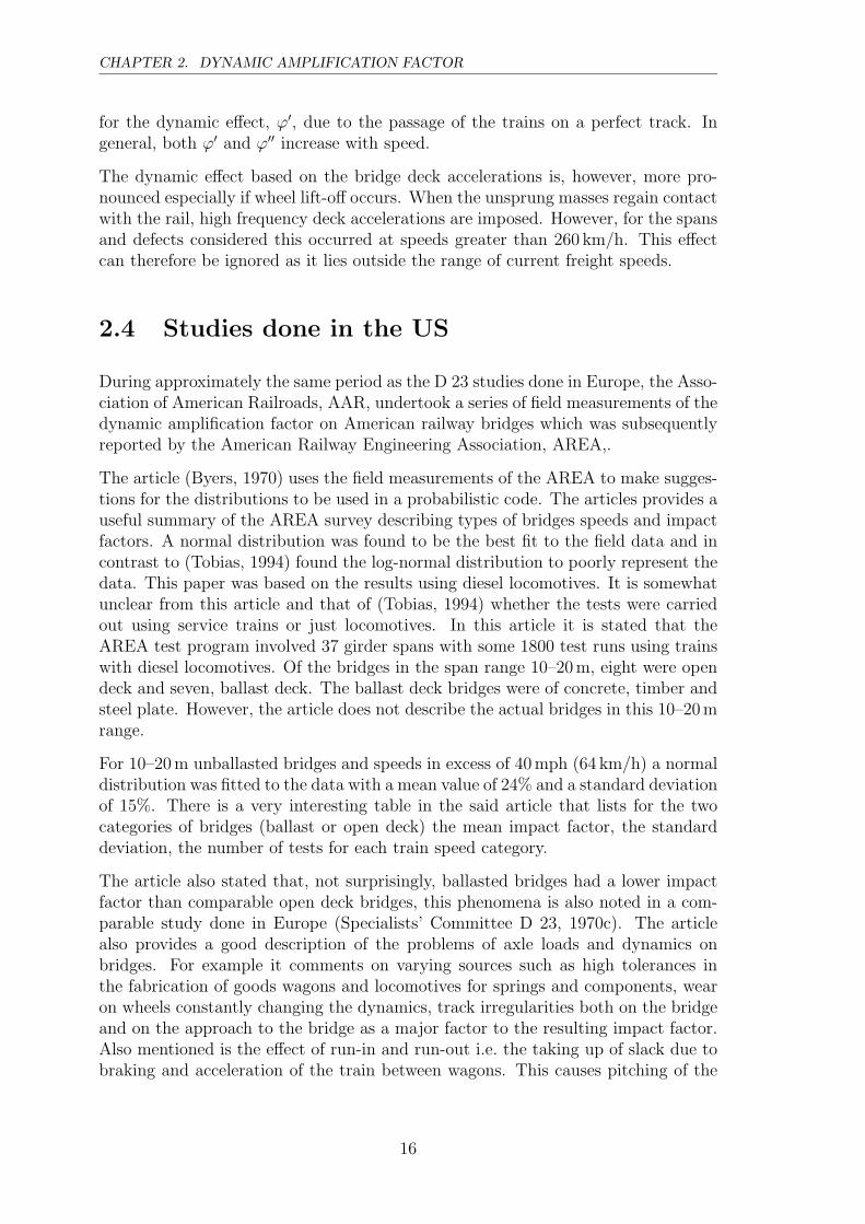
The Ph.D. thesis (Tobias, 1994) studies the fatigue evaluation of riveted steel rail-way bridges. The thesis presents Monte-Carlo traffic models for evaluating the loadeffects in riveted railway bridges for American conditions. It uses results of weigh-in-motion studies, locomotive and wagon types and train frequencies and configu-rations. In the thesis, the dynamic effect is found to closely follow a log-normaldistribution. In Figure 2.1, which is redrawn from (Tobias, 1994), the fitted dis-tributions are shown for the 9.1–18.3 m ballasted decks for different speed ranges.The properties of the fitted log-normal distributions are shown in the thesis for bothopen deck and ballasted bridges, for differing ranges of span and for the ranges oftrain speed shown in Figure 2.1.

17


0 5 10 15 20 25 30 35 400

0.05

0.1

0.15

0.2

0.25

Dynamic Effect [%]

Pro

bab

ilit

y < 32 km/h

32 - 64 km/h

64 - 96 km/h

96 - 128 km/h

128 - 160 km/h

Figure 2.1: Probability vs. dynamic effect for fitted log-normal distribution, for bal-lasted decks with spans between 9.1 and 18.3 metres. Redrawn from(Tobias, 1994).

2.5 Comparison of Results from the Described

Studies

In the following section, a comparison has been done between the dynamic effectobtained from the original D23 reports, the dynamic effect obtained using the re-fined method and the dynamic effects taken from (Tobias, 1994) for both ballastedand unballasted girder span bridges. See Appendix B for details of the Eurocodecalculations.

One problem encountered was the definition of the natural frequency. In the Eu-rocode, the natural frequency designated no, is the unloaded natural frequency ofthe bridge and according to these formulae have an upper and lower bound for eachbridge span. The definition of K is, apart from this frequency definition, the sameas in the D23 committee reports, compare (B.6) and (2.2). It was chosen to relatethe dynamic effects by a choice of span L and speed v. In one of the D23 committeereport (Specialists’ Committee D 23, 1970c) an estimation of the loaded naturalfrequency can be obtained using the following:

f ≈ 5.6√δ

(2.13)

where δ is the deflection due to the traffic plus the dead load, measured in cm whichyields f in Hz. In (Specialists’ Committee D 23, 1970c) a limiting value from a

18

2.5. COMPARISON OF RESULTS FROM THE DESCRIBED STUDIES

0 20 40 60 80 100 120 140 1600

0.1

0.2

0.3

0.4

0.5

0.6

0.7

0.8

Speed [km/h]

D23 mean value (2.9)

D23 95 % value (2.9–2.10)

D23 95 % value (2.3–2.4)

UIC limit values

USA ballast 95 %

USA ballast mean

USA unballast 95 %

USA unballast mean

ϕ

Figure 2.2: Dynamic effect according to the UIC leaflet method, the D23 reports(2.3) and (2.9) and finally the findings from USA for L = 10 m. Meanvalues and 95 % upper confidence limits are detailed.

Table 2.1: Listings of the bridge properties to Figures 2.2–2.3.

Span L Loaded frequency f Unloaded frequency range no Φ2

10 5.0 8.0 <= no <= 16.9 1.31

18 3.7 4.0 <= no <= 10.1 1.168

serviceability state requirement is used such that the deflection should be limited toL/800. Using this restriction as the limit case for δ and changing to metres yields:

f ≈ 5.6√L/8

(2.14)

where f is obtained in Hz provided L is inserted in metres. This value of f has thencontinuously been used when calculating the dynamic effects from the equations ofthe D23 committee reports, i.e. (2.3–2.10).

In Figures 2.2 and 2.3 a comparison has been made between the dynamic factoras calculated in accordance with the refined method of the UIC leaflet (good trackmaintenance), the original regression curves of the D23 final report and the Ph.D.thesis, based on the measurements done by the AAR. The figures show the cases ofa 10 m and a 18 m bridge, respectively. In the case of the UIC calculated effect boththe upper and the lower frequencies have been shown, so that the maximum of thesetwo values should be used in design. The mean value of the dynamic factor plusthe 95 % upper confidence limit has been shown for the dynamic effect calculatedusing the final equation of the D23 report, see (2.9–2.10). Also shown is the 95 %

19


0 20 40 60 80 100 120 140 1600

0.1

0.2

0.3

0.4

0.5

0.6

0.7

Speed [km/h]

D23 mean value (2.9)

D23 95 % value (2.9–2.10)

D23 95 % value (2.3–2.4)

UIC limit values

USA ballast 95 %

USA ballast mean

USA unballast 95 %

USA unballast mean

ϕ

Figure 2.3: Dynamic effect according to the UIC leaflet method, the D23 reports(2.3) and (2.9) and finally the findings from USA for L = 18 m. Meanvalues and 95 % upper confidence limits are detailed.

upper confidence limit calculated using (2.3–2.4) for steel bridges. The dynamicfactors calculated from the American studies are also shown with the mean andthe 95 % upper confidence limit drawn for both the ballasted and the unballasteddecks. These are easily identified as they appear as stairs, the original data beingcategorised into speed ranges.

As can be seen from the Figure 2.2, the 95 % upper confidence limit of the originalD23 regression curves almost coincide with both the upper limit according to theUIC 776-1R method and the 95 % upper confidence limit of the unballasted bridgesof the US study, at least for train speeds less than approximately 70 km/h. Forballasted bridges, the American study shows a maximum dynamic effect that isonly 0.25 and 0.11 for the 95 % upper confidence limit and the mean, respectively,which can be compared with the value of between 0.4–0.46 when using the methodof the UIC leaflet. From the US study only the 95 % upper confidence limit forunballasted decks produce the dynamic effects predicted by the UIC leaflet. Belowspeeds of 120 km/h, the 95 % upper confidence limits of the D23 findings and the95 % upper confidence limits of the US study on unballasted bridges are in goodagreement. This is not surprising as the regression curves of the D23 report werebased on the unballasted bridges stating the ballasted case to be more beneficial.The findings of the US study for ballasted bridges show a maximum value of thedynamic coefficient of 0.11 and 0.25 for the mean and the 95 % upper confidencelimit respectively, for the studied speed ranges.

The case of the 18 m span is shown in Figure 2.3. Again the 95 % upper confidencelimits of both the US unballasted bridges and the D23 regression curves are in good

20

2.6. SUMMARY AND COMMENTS

agreement. For speeds less than 120 km/h, the dynamic effect from the UIC leafletare in close agreement with the 95 % upper confidence limit of the ballasted bridgesof the US study. The mean value for the US ballasted bridges remains much smallerthan the UIC leaflet recommendations, especially under typical operating speeds forfreight trains of approximately 70–110 km/h.

This small comparison seems to suggest that the dynamic effect as proposed bythe UIC leaflet are in the order of the 95 % upper confidence limit at least forthe smaller span bridges and for normal freight operating speeds. Indeed in boththe UIC leaflet and in (Weber, 1998) it is stated that the given formula for ϕ′ isdescribed as representing the 95 % upper confidence limit, while the formulae forϕ′′ are described as an upper bound that may be exceeded by as much as 30 % forspecial cases of high train speeds and special vehicles. The wording for the propertiesof ϕ′′ are difficult to interpret and since there is no comment in the UIC leaflet thatgives either the mean values or the associated standard deviations it is impossibleto statistically describe the dynamic effects. Either of these quantities would besufficient to approximate a normal or a log-normal distribution.

For the larger of the two spans studied, the UIC leaflet recommendations producedynamic effects that appear to underestimate the 95 % upper confidence limit forthe unballasted bridges but remain above the mean value of the AAR findings forunballasted decks. For this span the UIC calculated dynamic effect is more in linewith the AAR 95 % upper confidence limit for the ballasted bridges. The AARtest show that the dynamic effect reached a maximum at speeds of approximately100–120 km/h for both the ballasted and the unballasted decks, at least within thespeed ranges considered.

The experimental results of the UIC findings and the AAR tests are in good agree-ment for the 95 % upper confidence limits of the unballasted bridges. It may there-fore be possible to use the AAR test results for the European case and assume thatthe dynamic properties of the US ballasted bridges are similar to the European. Thiswould therefore provide the required means and standard deviations for a statisticaldescription of the dynamic effects and also enable a distinction between ballastedand unballasted bridges. The means and standard deviations of the individual com-ponents ϕ′ and ϕ′′, however, remain elusive. The only report that separates theseparameters is (Specialists Committee D 128 RP4, 1976) and then only the meansand the standard deviations are shown in part I of the report, where only threetrains are considered. Also, these values contain a mixture of simulations from thefreight, passenger and high-speed train.

2.6 Summary and Comments

The European studies in the D23 report are based on field measurements of thedynamic response of actual railway bridges under the action of travelling locomo-tives. However, the subsequent reports from ERRI have widely been of a theoreticalnature with computer simulations forming the basis for the findings. The use of the

21


field data appears to have been abandoned in preference to computer simulationsand theoretical studies.

The track imperfections on which the UIC leaflet 776-1R are based have been usedthroughout these ERRI studies and used as a means of comparison. How theseimperfections relate to actual modern track standards and maintenance does notappear to be discussed, with the exception of the D 214 final report which statesthat this may be a source of saving when assessing existing railway bridges.

The dynamic effects of the UIC leaflet are approximately the 95 % quantiles althoughit is stated that these values may be exceeded in exceptional cases. The methodappears to generally overestimate the dynamic effect especially for ballasted bridges.

The European equations from the D23 report (2.9–2.10) may be suitable for use ina reliability method to describe the dynamic effect for unballasted bridges and forspeeds less than approximately 100 km/h, after which they appear to heavily over-estimate the values. The American studies are better, in that a distinction is madebetween ballasted and unballasted bridges. They could therefore be implemented ina reliability application to describe the dynamic factor.

Modern railway bridges have lower damping and natural frequencies than were an-ticipated at the time of the implementation of the UIC leaflet. This does not havea great significance for this study although it may be of interest to note for studiesdone on modern railway bridges.

22

Chapter 3

Earlier Swedish Building Codes

3.1 General

In order to study the possibility of upgrading older bridges, knowledge of the earlierbuilding standards and their format are essential. In this chapter some of the earlierSwedish standards will be presented at least to the extent used in this thesis. Priorto the introduction of the building codes (Statens Betong Kommitte, 1989a; StatensBetong Kommitte, 1989b; Statens Planverk, 1987) in the 1980’s, the Swedish build-ing code format was the allowable stress format. In the allowable stress format theloads are treated as being deterministic and there is no increase of the loads to allowfor the uncertainties inherent in them. However, it is recognised in this code formatthat there are uncertainties involved both for the material strengths and for theloading. In order to account for these uncertainties the actual material strengthsare decreased by divided by a factor greater than unity, thus yielding the allowablestress. However this factor or overall safety factor is not easily available within thecode format. Ascertaining the overall safety factor is more difficult than in the par-tial safety factor format and has therefore been extracted using assumptions whichwill be described in the relevant section.

After 1980 the code format changed to the partial safety factor format also known asthe Load and Resistance Factor Design abbreviated LRFD. In the post 1980 codesit is easy to see the partial safety factors used on both the loadings and the materialstrengths as they are clearly stated within the codes.

This chapter is split into two main parts, the first describing the material propertiesand the appropriate safety factor, either taken directly from the codes or assumed.The second part describes some of the static traffic load models on railway bridgesused in Sweden over the last century and the accompanying dynamic amplificationfactor or dynamic effect as appropriate.

23

CHAPTER 3. EARLIER SWEDISH BUILDING CODES

3.2 Reinforced Concrete

3.2.1 1980’s Swedish Codes

The code format from the post 1980’s has been the partial safety factor format.Between 1980 and the current day there has been several versions of the Swedishcodes for reinforced concrete. However, it has generally remained unchanged throughthese different versions, at least as regards values for partial safety factors andmaterial strengths of concrete and reinforcement bars. When the simple case ofonly the dead weight and the traffic live load is considered then, in the ultimatelimit state, the dimensioning criterion is expressed as

Rd ≥ Gd + Qd (3.1)

where R, G and Q are the bearing capacity, the load effect of the self-weight andthe load effect of the traffic live load respectively. The index d indicating the di-mensioning values of the aforementioned variables.

The above equation (3.1) can be rewritten to include the relevant partial safetyfactors:

Rk

ηcγmγn

≥ Gkγg + Qkγq (3.2)

where ηc takes into consideration the systematic difference between the strength ofa test specimen with that of the strength in the actual construction (Boverket, 1995;Statens Betong Kommitte, 1989a). the partial safety factors γm, γn, γg, γq are thesafety factor for the material, the structure’s safety class, the self-weight and theimposed load respectively. The index k is used to indicate the characteristic values.

3.2.2 Swedish Concrete Code 1949 and 1968

During the late 1940’s and the late 1960’s the building codes for structural concretewere (Kommunikationsdepartementet, 1951) and (Statens Betong Kommitte, 1968),respectively. As mention earlier the code format of this period was the allowablestress format which can be expressed, when only the self-weight and the traffic loadare considered, by the following:

Rall ≥ Gd + Qd (3.3)

where Rall is the allowable strength of the material. Gd and Qd are the dimensioningvalues as described above. Their is no distinction between characteristic values anddimensioning values in this code format. The safety factors are not stated in thecodes and have therefore been induced. If one attempts to include the safety factorsthat are implicit in the expression for Rall we obtain

Rk

γinf

= Rall (3.4)

24

3.2. REINFORCED CONCRETE

where γinf in this case is the overall safety factor, Rk is the unstated characteristicstrength. The index inf is used to indicate that the safety factor has been inferred.

The case of the concrete compressive strength K 400 has been considered. Thenotation K 400 is from the code (Statens Betong Kommitte, 1968) and is assumedto be equivalent to the concrete defined in the later codes (Statens Betong Kommitte,1989a; Statens Betong Kommitte, 1989b; Boverket, 1995) as K 40. The later codesprovide details of the characteristic compressive strength, fcck and for this concreteis equal to 28.5 MPa1. The allowable compressive strength in bending for the K 400concrete, according to both the 1968 and the 1949 concrete codes (Statens BetongKommitte, 1968; Kommunikationsdepartementet, 1951), is 12.5 MPa for what isreferred to as the normal load case, which is equivalent to the serviceability limitstate, SLS. This value should be increased by 20 % for the exceptional load case,equivalent to the ultimate limit state, ULS. Re-arranging (3.4) and inserting theabove values produces an overall safety factor in bending for concrete given by:

γinf = 28.5/(12.5 · 1.2) = 1.9 (3.5)

Similar assumptions are employed to infer the overall safety factor for the reinforce-ment steel. The reinforcement steels chosen are Ks 40 and Ks 60 according to thenotation used in (Boverket, 1995; Statens Betong Kommitte, 1989a), which are com-mon reinforcement steel qualities in bridge building. These steels are assumed to beequivalent to the steel qualities of (Kommunikationsdepartementet, 1951; StatensBetong Kommitte, 1968), which also use the same notation. According to (Bover-ket, 1995) the characteristic yield strengths, fyk in tension are approximately 400and 600 MPa respectively for Ks 40 and Ks 60 steel2. According to the concrete codeof 1968 (Statens Betong Kommitte, 1968) the highest allowable tensile stresses are220 MPa and 330 MPa for the two steel qualities, respectively. The allowable ten-sile stress varies depending on the bar diameter, however, using the highest valuesproduce the lowest assumed safety factors which will in turn produce conservativeresults of the reliability analysis to be performed at a later stage. For the case ofthe 1949 concrete code (Kommunikationsdepartementet, 1951) only the steel qualityKs 40 is listed and this is given the same value as above i.e. 220 MPa. Again thesevalues should be increased by 20 % for the case of exceptional loading. As before,inserting these values into (3.4) and re-arranging yields:

γinf = 400/(220 · 1.2) = 600/(330 · 1.2) = 1.52 (3.6)

The characteristic strength of concrete changed from the 10 % quantile to the 5 % in1986 according to (Banverket, 2000). However there is also an equation in this hand-book on adjusting the characteristic concrete strength due to the general increasein strength of concrete with age. For bridges built before 1986 it is suggested that

1According to (Boverket, 1995) the characteristic concrete compressive strength is defined as0.85 of the 5 % quantile of the cylindrical compression strength. The factor 0.85 is intended totake into account long term effects.

2According to (Boverket, 1995) the values represent the 5 % quantile of the upper yield pointor the 0.2-percent offset method.

25


Table 3.1: Steel properties according to (Kommunikationsdepartementet, 1948). Al-lowable stresses are for exceptional loads i.e. equivalent to ULS.

Lower yield strength Ultimate strength Allowable stressGrade fyk [MPa] fuk [MPa] fpt [MPa]St 38 220 ≥ 390 135St 44 260 460 ≤ fuk ≤ 500 160

the characteristic strengths be adjusted by an increase of 15 % for the hardening ofthe concrete with age but a decrease of 2 MPa to account for the change from the10 to 5 % quantile. This would increase the characteristic strengths of the concreteclasses considered in this thesis. The effect then of changing from the two quantilevalues has been ignored in this thesis as the concrete hardening with age appearsto more than compensate for this change. This therefore ignores the increase instrength that the concrete undergoes and this thesis assumes, conservatively, thatthe 5 % quantile represents the characteristic values for the concrete strength.

3.3 Structural Steel

3.3.1 1980’s Swedish Codes

The format for the Swedish steel codes of approximately 1980 was the partial safetyfactor format. The formulation in the ultimate limit state was similar to that of theconcrete code, see (3.2). The characteristic strength is defined in (Boverket, 1997)as representing the 1 % quantile of the upper yield point. The material partial safetyfactors are tabulated in Table 3.2.

3.3.2 1938 Swedish Code for Structural Steel

Again the format of this code (Kommunikationsdepartementet, 1948) is the allow-able stress format. Structural steel grades often used for railway bridges of the timeare St 37 and St 44, using this code’s notation. Within the text of the code the loweryield point i.e. the limit of proportionality is used to define the material strengthand the minimum value for the steel grades are listed in Table 3.1 as fyk. It is alsostated in the code that a 5 % deviation from this value is allowed for test results.Another method of classifying the grade of the steel through testing according to(Kommunikationsdepartementet, 1948) is to see if the ultimate tensile strength, fuk,lie within the limits shown in Table 3.1. The allowable stress, denoted fpt, for aslenderness ratio of zero is listed in Table 3.1. This slenderness ratio was chosen asit produces the safety factor without the any inherent safety factor against buck-ling. It therefore produces the smallest value and will lead to the most conservativecalculation in the forthcoming reliability analysis.

The inferred overall safety factors were then assumed to be given by (3.4) by inserting

26

3.4. SUMMARY OF MATERIAL PROPERTIES

Table 3.2: Summary of safety factors, the approximate code year and the valuesof the quantiles which the material strengths are supposed to representaccording to the appropriate code.

Year γinf ηcγm γna Quantile %

Concrete(compression)

1980– – 1.5 1.2 51968 1.9 – – 51949 1.9 – – 5

Reinforcement Steel(tension)

1980– – 1.15 1.2 5 b

1968 1.52 – – 51949 1.52 – – 5

Structural Steel(tension)

1980– – 1.0 1.2 11938 1.63 – – 1

aThe values given for γn apply to bridges.bThere is a double conversion here from the 1 % quantile of the lower yield point (from Swedish

testing standards) to the 5 % quantile of the upper yield point cf. (Statens Betong Kommitte,1989a; Boverket, 1995). The latter being the definition of the characteristic strength.

the values of fpt and fyk which yield

γinf = 220/135 ≈ 260/160 ≈ 1.63 (3.7)

3.4 Summary of Material Properties

Table 3.4 is a summary of the material properties assumed throughout this thesis.The year refers to the approximate year of the code, the safety factors are thestated or the inferred safety factors used on the material properties. Also listed arethe values of the quantiles which the material strengths are supposed to representaccording to the appropriate code.

3.5 Traffic Load Models

3.5.1 Swedish Load Model 1901

According to (Paulsson et al., 1998) many of the older bridges in Sweden were builtbetween 1900 and 1920 to the load model from 1901. The traffic load model is shownin Figure 3.1 and the equivalent uniformly distributed load is shown in Table 3.3together with the dynamic coefficient for a train speed of approximately 90 km/h.The article states that the load Model A was intended for lines with heavier freighttraffic and Model B for normal lines. It is also noted that there are bridges designedto an even lighter load called Model C and that some of the routes in Sweden containlines with a mixture of bridges designed to these different specifications.

27


Table 3.3: Uniformly distributed load and the dynamic coefficient for a train speedof 90 km/h from 1901. Reproduced from (Paulsson et al., 1998).

Theoretical Load Model Load Model Dynamicspan A B coefficient(m) (kN/m) (kN/m) (%)1.3 308 277 752.3 174 157 653.3 158 143 554.3 158 143 485.3 147 133 406.4 143.5 129 337.4 136.5 123 298.5 128 115 269.5 120 108 2410.5 113.5 104 2211.5 107 101 2012.5 103 94.5 1914.5 100 91 1815.6 96.5 90 1716.6 96.3 88.5 1718.6 93.5 85.5 1619.6 92 84.5 1620.6 90 83 1522.7 89 81 14

The article provides a concise and informative summary of the problems facing theSwedish National Railway Administration in its work to increase allowable axle loadson exiting railway bridges. The article also states that in 1919 the train load modelwas modified and that the dynamic coefficient was increased.

In this thesis Load Model A is studied whenever reference is made to this year,together with the dynamic coefficient of Table 3.3.


The revised load models can be found in (Simonsson et al., 1929) although theyare very similar to the models shown in Figure 3.1 except for a minor alterations inthe axle spacings. The dynamic coefficient changed substantially and is detailed in(Simonsson et al., 1929) as being

ε =1000

13 + 0.7Le

(3.8)

which applies for an intended maximum train speed of 100 km/h and where theeffective length Le is inserted in metres, the dynamic coefficient ε is obtained in %.

28

3.5. TRAFFIC LOAD MODELS

18 t 18 t 18 t

1.4 1.7 1.7 1.8

Tender 54 t6.6

18 t 18 t 18 t

1.4 1.7 1.7 1.8

Tender 54 t6.6

15 t

2.0 2.7 1.4 2.7

20 t 20 t 20 t 20 t

1.4 1.4

11.6Locomotive 95 t

15 t

2.0 2.7 1.4 2.7

20 t20 t 20 t20 t

1.4 1.4

11.6Locomotive 95 t

1.6

20 t

2.0

20 t 20 t

2.0 1.6

7.2Ore wagons 60 t each

1.6

20 t

2.0

20 t 20 t

2.0 1.6

7.2

16 t 16 t 16 t

1.4 1.6 1.6 1.8

Tender 48 t6.4

16 t 16 t 16 t

1.4 1.6 1.6 1.8

Tender 48 t6.4

13 t

2.0 2.6 1.4 2.5

18 t18 t 18 t18 t

1.4 1.4

11.3Locomotive 85 t

13 t

2.0 2.6 1.4 2.5

18 t18 t 18 t18 t

1.4 1.4

11.3Locomotive 85 t

1.6

14 t

3.3

14 t

1.6

6.5

1.6

14 t 14 t

3.3 1.6

6.5Loaded wagons 28 t

12 t 12 t 12 t

1.3 1.6 1.6 1.8

Tender 36 t6.3

12 t 12 t 12 t

1.3 1.6 1.6 1.8

Tender 36 t6.3

7 t

1.4 2.4 1.4 2.6

14 t14 t 14 t14 t

1.4 1.4

10.6Locomotive 63 t

7 t

1.4 2.4 1.4 2.6

14 t14 t 14 t14 t

1.4 1.4

10.6Locomotive 63 t

1.6

14 t

3.3

14 t

1.6

6.5

1.6

14 t 14 t

3.3 1.6

6.5Loaded wagons 28 t

Load Model A. Locomotive with 20 tonnes axle weight

Load Model B. Locomotive with 18 tonnes axle weight

Load Model C. Locomotive with 14 tonnes axle weight

Figure 3.1: The traffic load models from the Swedish codes of 1901. All measure-ments are in metres and weights are in tonnes. Redrawn from (Paulssonet al., 1998).

This book also states that the dynamic coefficient can be decreased for concreteand reinforced concrete bridges when a fill material is present whose height exceeds1.0 m, measured from underside of the rail. The revised dynamic coefficient is statedas being

εh =6 − h

5ε (3.9)

where ε is obtained from (3.8) and h is the height of the fill in metres.

The book also states that the superstructure of the bridge may or may not containballast. However, it also comments that the case without ballast is the more commonas the relatively large extra weight of the ballast increases the cost of the bridge. Itis therefore assumed in this thesis that the majority of the bridges built around thisperiod do not contain ballast.

3.5.3 Swedish Load Model 1940’s

The traffic load models used in Sweden during the 1940’s are detailed in (Kommu-nikationsdepartementet, 1948) and reproduced in Figure 3.2. There are also tablesin this document which give details of the maximum static moment, the maximumshear force and the equivalent uniformly distributed load for the case of simply sup-ported beams, which correspond to the loading models A and B. Part of the tablefor the case of load model A is reproduced in Table 3.4

The dynamic coefficient, ε in %, to be used is also specified in this document and is

29


18 t 18 t 18 t

1.4 1.6 1.6 1.8

Tender6.4

18 t 18 t 18 t

1.4 1.6 1.6 1.8

Tender6.4

15 t

2.0 2.6 1.5 2.5

20 t20 t 20 t 20 t

1.5 1.5

11.6Locomotive

15 t

2.0 2.6 1.5 2.5

20 t20 t 20 t 20 t

1.5 1.5

11.6Locomotive

Loaded Wagons 8.5 t/mUnloaded Wagons 1.0 t/m

UDL

Load Model A

1.4 1.6 1.6 1.8

Tender6.4

1.4 1.6 1.6 1.8

Tender6.4

2.0 2.6 1.5 2.5

16.2 t 16.2 t 16.2 t13.5 t 18 t 18 t 18 t 18 t

1.5 1.5

11.6Locomotive

2.0 2.6 1.5 2.51.5 1.5

11.6Locomotive

Loaded Wagons 5.0 t/mUnloaded Wagons 1.0 t/m

UDL

Load Model B

16.2 t 16.2 t 16.2 t13.5 t 18 t 18 t 18 t 18 t

Figure 3.2: The traffic load models from the Swedish codes of 1938. All measure-ments are in metres and weights are in tonnes. Redrawn from (Kommu-nikationsdepartementet, 1948).

Table 3.4: Maximum moments, without the dynamic coefficient, for a simply sup-ported beam exposed to Load Model A from the Swedish code of 1938.Reproduced in part from (Kommunikationsdepartementet, 1948).

Span L Max moment(m) (kNm)1 502 1003 1694 3005 4506 6197 8168 10149 123010 146812 194315 278420 459725 6922

given by the following formula:

ε =1765

20 + Le

(3.10)

where Le is the theoretical length i.e. distance between zero points of the load effectto be studied. This formula (3.10) applies to a maximum speed of 100 km/h and amore general formula is also given in the document by:

ε =370 + 15.5(v − 10)

20 + Le

(3.11)

30


1.6 1.6 1.6

Locomotive 11.2

25 t

1.6 1.6 1.6 1.6

25 t 25 t 25 t 25 t 25 t

1.6 1.6 1.6

Locomotive 11.2

25 t

1.6 1.6 1.6 1.6

25 t 25 t 25 t 25 t 25 tLoaded Wagons 8.5 t/mUnloaded Wagons 1.5 t/m

UDLLoaded Wagons 8.5 t/mUnloaded Wagons 1.5 t/m

UDL

1.6 1.6

Load Group 1

25 t

1.6 1.6

25 t 25 t 25 t 25 t

1.6 1.6

Load Group 2

20 t

1.6

20 t 20 t 20 t

Load Model Type F

Figure 3.3: The traffic load models from the Swedish codes of 1960. All measure-ments are in metres and weights are in tonnes. Redrawn from (Kommu-nikationsdepartementet, 1961).

where v is the maximum speed of the line in km/h and Le is the theoretical distance,in metres, between zero points as before. No distinction is made between a bridgebuilt with or without ballast in this load model, as regards the dynamic amplificationfactor.

In this thesis the Load Model A has been used together with the dynamic effectgiven by (3.10) whenever reference is made to the year 1940.


The traffic load model for the 1960 Swedish code is detailed in (Kommunikations-departementet, 1961) and reproduced in Figure 3.3. The Load Model F is intendedfor the heavy haul lines of the time. The traffic load could be reduced to 85 % ofthe load effect from Load Model F for other normal gauge lines or be designed toLoad Group 1 (see Figure 3.3) whichever gave the greatest effect.

The dynamic coefficient, in %, can be calculated according to (Kommunikationsde-partementet, 1961) from the following formula

ε =2200 + 11Le

25 + Le

(3.12)

where Le is the effective length in metres. There is an accompanying table todecide the effective lengths for different types of constructions and different partsof a construction, for a simply supported beam the effective length is the spanlength of the beam. There is also another table to be used in conjunction with thedynamic coefficient to take into account the type of track and its joints. This tableis reproduced in Table 3.5. However, in the main text it is stated that for the cases1, 2 and 3a the dynamic coefficient should not be less than 20 %.

For this study the case of a welded track with a ballast bed of between 0.4–0.6 mhas been considered, i.e. case 3a of Table 3.5. This will yield results on the conser-vative side as it assumes the lowest dynamic coefficients were used at the time ofconstruction, if one disregards the case of high ballast or fill in excess of 0.6 m.

31


Table 3.5: Dynamic coefficient for different types of track and track joints. Repro-duced from (Kommunikationsdepartementet, 1961).

Type of rail jointType of track Bolted Welded

1 Rail placed with direct contact tothe superstructure

1.1ε 1.0ε

2 Rail placed on wooden sleeperswhich are themselves in directcontact with the superstructure

0.9ε 0.8ε

3 Continuous ballast bed or fill withmean height h, measured from theunderside of the rail

a. h =0.4–0.6 m 0.8ε 0.8εb. h ≥ 6 m 0 0c. 0.6 < h < 6.0 m Dynamic coefficient is

linearly proportional betweenthe values in 3a and 3b

0.8 0.8no limitation no limitation

qvk = 8 t/m qvk = 8 t/m

Qvk= 25 t 25 t 25 t 25 t

1.6 m1.6 m1.6 m

Figure 3.4: The characteristic vertical loads referred to as UIC71 in (Banverket,1997) and Load Model 71 in (CEN, 1995).

Whenever reference is made to 1960 in the following chapters of the thesis LoadModel F has been used without any reduction. In this context, the dynamic factorused has been calculated according to case 3a of Table 3.5 and using (3.12).


The load models that were used for the design of railway bridges in Sweden afterapproximately 1980 and until recently, are shown in Figures 3.4 and 3.5. Thesemodels represent the static vertical characteristic loads and in the Swedish code ofpractice a bridge should be designed for these two load models, whichever gives riseto the worst case for the parameter under design. The loads should be placed at themost unfavourable position for the structural component and load effect in question.

The UIC leaflet (UIC, 1974) provides a table in one of its appendices of the maximummoment in a simply supported beam, together with its position, when loaded with

32


25 m 25 m7 m

qvk

=150 kN/m qvk

=150 kN/m

Figure 3.5: The characteristic vertical loads for heavy rail traffic, referred to as SW/2in both (Banverket, 1997) and (CEN, 1995).

Figure 3.6: A typical wagon used for transportation of a heavy load, a Uaai-z repro-duced from (StatensJarnvag, 2000).

Load Model 71. There is, however, an allowance in the codes of practice (Banverket,1997; CEN, 1995) for the point loads to be distributed when a minimum heightof ballast is present. The code moments used in this thesis, therefore, assume aballasted track and adopt a simplified method where the point loads are replaced byan equivalent UDL of 156 kN/m over a length of 6.4 m. These moments are lowerthan those of (UIC, 1974) and will therefore yield higher moment ratios, i.e. resultson the conservative side.

The UIC71/Load Model 71 load is meant to represent normal traffic on internationallines and has been used, in Sweden, in conjunction with the maximum allowable axleweight of 22.5 tonnes and a maximum allowable weight per metre of 8 tonnes forthe best class of line.

The SW/2 load comes from the German Schwerlast meaning heavy load. Thistype of load is typically for the transportation of large loads such as turbines, largeindustrial machines. The loads are often known exactly and the speeds of the trainsare often limited to 30 km/h. In Sweden, the Swedish National Rail Administration,(Banverket), individually check the capacity of the bridges along a proposed routebefore permission is granted for the transportation of such loads. A typical wagonfor such a load is shown in Figure 3.6. A comparison of Figures 3.5 and 3.6 revealsthe similarities between the actual load and the load model, at least in format if notnumerically.

In order to obtain the design loads these characteristic static vertical traffic loads are

33


Table 3.6: Partial safety factors γq for traffic loads.

Swedish Code Eurocode

UIC71 SW/2 Load Model71 SW/2

γq 1.4 1.2 1.45 1.2

multiplied by a partial safety factor for variable loads and by a dynamic amplificationfactor. The respective partial safety factors for the two load models are tabulatedin Table 3.6 for both the Swedish and the European code of practice.

According to the simplified rules of (CEN, 1995; Banverket, 1997) the dynamicamplification factor for carefully maintained track is given by the following equation:

Φ2 =1.44(√

LΦ − 0.2) + 0.82 (3.13)

where LΦ is the determinant length in metres. In the Swedish code of practicethere is a limitation that 1.05 ≤ Φ2 ≤ 1.67 while in the Eurocodes the equivalentlimitation is 1.00 ≤ Φ2 ≤ 1.67. The definition of the effective lengths vary somewhatbetween the Swedish code and the European code (Kindberg and Rydberg, 1997),although for the studied case of simply supported beams they are the same.

The dimensioning load effect of the load models illustrated in Figures 3.4 and 3.5multiplied by the dynamic amplification factor of (3.13) have been used in futureanalysis as a denominator in order to produce a normalised load effect. It should bestressed that the load effect obtained in this manner is purely from the characteristicload and the dynamic effect. The Swedish code of practice has been used for thispurpose, taking into consideration the partial safety factors when determining whichof the load models will be the dimensioning one but not using them. The momentfrom this load model has been used throughout this thesis and has been given thenotation Muic71Φ. Since the load effect considered has been the moment at mid-spanthen this traffic load effect has also been referred to as the nominal load effect, Qn

in the reliability chapters.

3.5.6 Comparison of Traffic Load Models 1901–1971

A comparison of the dynamic amplification factors for the four Swedish codes ofpractices studied, are shown in Figure 3.7. It is interesting to note that the dynamicfactor increased substantially between 1901 and 1940 and remained at this levelduring the 1960’s before being reduced back closer to the original 1901 code rules.These changes are interesting when it is borne-in-mind that the vehicle and tracktechnology during this period has undergone many changes i.e. from being boltedto continuously welded rail, from steam locomotives inducing extra dynamics fromhammer blows to the modern day suspensions (at least for some vehicles) and fromrails fastened immediately to the superstructure (or via wooden sleepers) to essen-tially ballasted bridges. These positive effects (i.e. generally act to decrease the

34


0 5 10 15 20 25 30 35

1.1

1.2

1.3

1.4

1.5

1.6

1.7

1.8

1.0

1971

1901

19401960

Φ

L [m]

Figure 3.7: Comparison of the dynamic amplification factor, Φ, used in some of theSwedish railway bridge codes during the last century.

Table 3.7: Dynamic mid-span moment for the studied years as a fraction of the 1971dynamic mid-span moment.

Span L in metresCode Year 4 8 10 13 20 30

1960 1.1211 1.2075 1.2487 1.2874 1.1042 1.13091938 0.9917 0.9545 0.9451 0.9209 0.7426 0.72161901 0.9384 0.8027 0.7523 0.7177 0.6074 0.5962

dynamic effect) have, however, been accompanied by a general increase in allowablevehicle speed, at least for passenger trains, which generally tend to increase thedynamic effect.

A comparison of the mid-span moment due to the characteristic loads of the variousSwedish codes can be seen in Figure 3.8 for the cases excluding and including thedynamic effect.

35


0 5 10 15 20 25 30 350

2

4

6

8

10

12

14

16

18

1971

190119401960

L [m]

Mom

ent

[MN

m]

(a) Static mid-span moment

0 5 10 15 20 25 30 350

5

10

15

20

25

1971

190119401960

L [m]

Mom

ent

[MN

m]

(b) Dynamic mid-span moment

Figure 3.8: Comparison of the characteristic mid-span moment vs. span from someof the load models of the Swedish railway bridge codes during the lastcentury.

36

3.6. COMBINATIONS OF MATERIAL PROPERTIES AND LOAD MODELS

Table 3.8: The combination of load models and material standard studied in thisthesis, together with a definition of the years used for identification.

Material Definition Year Traffic Load Model Material Code Yearcf. Table 3.2

Concrete

1980 UIC 71 or SW/2 1980(cf. section 3.5.5)

1960 Load Model F 1968(cf. section 3.5.4)

1940 Load Model A 1949(cf. section 3.5.3)

StructuralSteel

1980 UIC 71 or SW/2 1980(cf. section 3.5.5)

1960 Load Model F 1938(cf. section 3.5.4)



3.6 Combinations of Material Properties and Load

Models

In the following chapters of the thesis the years 1901, 1940, 1960 and 1980 are usedto present the results. The definitions of the use of these years are presented here.

Table 3.8 shows the combination of load models and material codes used whendefining the above mentioned years. For example, when referring to the year 1980in the forthcoming text, this means that the dimensioning load was assumed to bethe dimensioning case of the UIC 71 or the SW2 load model including its associateddynamic factor Φ2. The material code was that from 1980, see Table 3.2 for thepartial safety factors for this year. Similar definitions are included for each yeardefinition. All traffic load models include the allowance for dynamic effects.

As regards the material properties of the constructional steel, only the code (Kom-munikationsdepartementet, 1948) was used in order to imply the overall safety factorof 1.63, see Table 3.2, which was used throughout for the allowable stress code for-mats, i.e. prior to approximately 1980. This assumed safety factor was then usedin combination with the different load models prior to 1980 to produce the differentresults. This is obviously incorrect and safety factors should be obtained or inferredfor these code years. However, as regards concrete the inferred safety factors didnot change from the 1949 code to the 1968 code and it may be reasonable to assumethat the safety factors for steel constructions did not change significantly during thisperiod.

37

Chapter 4

Reliability Theory and Modelling

4.1 General

In this chapter, reliability theory and the methods of assessing the safety or relativesafety of a structure are discussed. The first part of the chapter, sections 4.2–4.7, is ashort introduction into the subject of reliability theory and illustrates the iterationprocedures used to estimate the design point and hence the safety index. Theseparts of the chapter are taken from various textbooks, e.g.(Thoft-Christensen andBaker, 1982; Melchers, 1999; Madsen et al., 1986), and can therefore be skippedby the reader familiar with the concept of reliability theory. These early sectionsare only intended as an introduction to the basic concepts, an interested reader isreferred to the aforementioned textbooks. Section 4.8 and onwards deal with thespecific situation as it relates to the work done in this thesis.

The textbooks mentioned provide a sound theoretical background on this subject,however the publications by The Nordic Committee on Building Regulations (NKB)(NKB, 1987) and that by The Joint Committee on Structural Safety (JCSS) (JCSS,2001) are of more practical help for the engineer.

4.2 Introduction

Structures such as bridges, our places of work and apartment buildings need to besafe, we do not expect a bridge to collapse when we drive over it or a building tofall down while sitting at home with our families. However buildings can never bebuilt to be totally safe, there must always be a risk of failure. Building a totally safebuilding would mean using an infinite amount of resources in order to withstandan infinitely large load, this would be undesirable. The risk of failure of a buildingshould be very low, one does not expect to be exposed to the same degree of risksitting at work in the office as a mountaineer faces climbing the north face of MountEverest.

Loads on buildings vary with time and are rarely known in advance, they can be

39

CHAPTER 4. RELIABILITY THEORY AND MODELLING

described by stochastic processes. Even the geometry and material strengths of abuilding vary and can therefore be described as stochastic variables. If hundredsof identical buildings were built beside one another the thickness e.g. of the floorslab will vary between the buildings and so would the material strengths of anyequivalent sections within the buildings. The built structure is therefore only onerealisation of the unlimited number of possible outcomes.

Safety and reliability theory is a method based on mathematical statistics wherebythe material strengths, the loading process with time and model uncertainties can bedescribed by stochastic processes and variables and statements can be made aboutthe safety or the mean time to failure of a structure.

The origins of safety and reliability theory come from the aero- and manufacturingindustries and from electronic components where it was of interest to establish thefailure rate of certain components or system of components. The field of expertisewas further used in the space industry where a high level of reliability was essentialand also in computers and telecommunications.

The structural engineer, as opposed to the electronic engineer, does not have theluxury of being able to build hundreds of exactly similar structures and test them tofailure. Indeed each structure is unique, however the theory of safety and reliabilityprovides a rational treatment for the assessment of the safety of a structure.

The codes for design of structures are deterministic in there nature. The load on astructure has a certain upper value known as the characteristic value. The materialstrength parameter has a certain lower value, these parameters are multiplied byfactors of safety in the load case and divided by factors of safety in the materialparameter case. These safety factors allow for the uncertainty involved in thesecharacteristic values and for the uncertainty of the models used, i.e. testing thecube strength to ascertain the compressive strength of the concrete in the structure.The newer codes, however, do allow for an assessment of the uncertainties usingmore probabilistic methods.

Mathematical statistics is an integral part of structural reliability. The followingchapter assumes that the reader is familiar with basic statistics, however, the theoryof extremes and the methods of parameter estimations have been given a chapter oftheir own, see Chapter 5.

The aim of this chapter is to present the main parts of structural reliability usedin this work. Although most of what is written is collected from the followingreferences it is included here partly for the sake of completeness, partly becauseit is essential for understanding the way in which simulation results are handledin later chapters and also to recognise the fact that for many civil engineers thissubject is often overlooked in a basic education. For a more detailed understandingof the subject, however, the reader is advised to read (Thoft-Christensen and Baker,1982) which provides a good introduction into the subject as does (Schneider, 1997)and (NKB, 1996a; NKB, 1996b; NKB, 1987). For a more detailed explanationof the theory see (Madsen et al., 1986). A more intricate coverage of the theoryis provided in (Ditlevsen and Madsen, 1996). However, in this authors personal

40

4.3. FUNDAMENTALS

opinion (Melchers, 1999) was the best of these books, at least for the basics, as itmanaged to cover the main points of the subject in a clear and concise manner.

4.3 Fundamentals

The basis for this theory is that the variables influencing the strength and loadingof a structure can be described by stochastic variables, shortened to s.v. or by astochastic process. The variables affecting the strength are often denoted by thestochastic variable R where R is a function of several other s.v. such as the modulusof elasticity E, the area of the cross-section A or the flexural strength in bending fb.Generally, the notation used throughout this chapter is that the stochastic variablesare shown as capitals while numerical values or outcomes such as sample values aredenoted with small letters, compare X and x. This may be new to some readers tothink of say the cross-sectional area of a floor slab as being a variable but one mustimagine that although a drawing specifies a certain dimension. If we were to buildseveral hundred of these floor slabs to the same drawing specifications the resultingfloor slabs will of course have a variation in thickness.

A structures reaction to a load is referred to as a load effect, e.g. the moment thatarises from a traffic load at a section in a bridge or the deflection created in astructure from a load. The load effect is often denoted by S and can arise from avariety of loads such as those from wind loading W , traffic loading Q, self-weight G,etc.

In the ultimate limit state, the safety margin denoted M , can in many cases bedefined by the following:

M = R − S (4.1)

and for the structure to be safe M ≥ 0. Equation (4.1) appears fairly innocuous,but we should remember that M , R and S are all s.v. so that the equation has aninfinite number of outcomes. Using the examples of material strength parametersand load effects from above, (4.1) becomes

M(E,A, fb, ...,W,Q,G, ...) = R(E,A, fb, ...) − S(W,Q,G, ...) (4.2)

In general terms the s.v. of E,A, fb,W,Q,G, ... can be described as X1, X2, ..., Xn

so that (4.2) becomes

M(X1, X2, ..., Xn) = R(X1, X2, ..., Xn) − S(X1, X2, ..., Xn) (4.3)

All the s.v. X1, X2, ..., Xn, known as the basic variables, will not necessarily appearin both S and R. However some will e.g. the thickness of a beam will act as astrength parameter but also in the form of the self-weight as a load parameter.

The limit state function or failure function, denoted g(xi) is a function that splitsthe x-space into a safe set S and a failure set F . The surface that divides these tworegions is the limit state surface or failure surface LX . Expressed mathematically

41


yields

g(xi) > 0, xi ∈ S (4.4a)

g(xi) = 0, xi ∈ LX (4.4b)

g(xi) < 0, xi ∈ F (4.4c)

The safety margin, M , introduced earlier is the s.v. obtained from replacing theparameters xi with the s.v. Xi in the limit state function such that

M = g(Xi) (4.5)

The above form of the safety margin, as expressed in (4.1) is typical of the ultimatelimit state. The safety margin does not always follow this form and the function gmay take any form provided that M ≤ 0 corresponds to a failure state and M > 0to a safe state. In the serviceability limit state a serviceability requirement for thedeflection of a beam of span l may be

S

R≤ l

300(4.6)

which expressed in the limit state form will yield a safety margin such that

M =l

300− S

R(4.7)

A load can be defined as a permanent or a variable load. The self-weight of astructure being described as a permanent load while traffic and wind loads arevariable loads as they are time dependent.

Structural reliability theory is broken up into three levels with increasing order ofcomplexity.

• Level I. This level regards the different variables as a single value usually themean or some characteristic value e.g. the 5 % quantile. This is the level usedfor most design work under the most current codes of practice. At this levelit is not possible to make statements about the probability of failure of astructure.

• Level 2. At this level the stochastic variables are represented by two proper-ties: the mean value and the variance and where necessary sometimes eventhe covariance. This method provides an approximation of the probability offailure.

• Level 3. For a level 3 analysis it is assumed that information is known thatfully describes the entire distributions for all the different stochastic variablesinvolved in the analysis. Given that these assumptions are correct it is possibleto make statements regarding the precise value for the probability of failure.

42

4.4. THE FUNDAMENTAL RELIABILITY CASE

4.4 The Fundamental Reliability Case

The basic reliability problem is that of the two dimensional case where the resistanceR and the load effect S are each described by one stochastic variable. The probabilitydistribution function for the resistance and the load effect are given by fR(x) andfS(x), respectively. For the sake of simplicity let us consider the case of a singlemember or a particular section, so that failure is defined when the load effect S isgreater than or equal to the resistance R. The probability of failure of this particularmember or section will therefore be:

pf = Prob (R ≤ S)

= Prob (R − S ≤ 0)(4.8)

or in general termspf = Prob [ g(R,S) ≤ 0] (4.9)

where g(r, s) is the limit state function. This probability can be defined in terms ofthe joint distribution function fR,S(r, s) by the following double integral

pf =

∫F

∫fR,S(r, s)dr ds (4.10)

where F indicates the failure domain.

In the event that the variables R and S are independent then (4.10) can be simplified,using the relationship fR,S(r, s) = fR(r)fS(s). The two distributions of S and R canthen be treated independently. The probability of failure is the probability that theload S will adopt a value between x and x+ dx while at the same time the strengthR takes on a value less than or equal to x and then summed for the entire range ofpossible x values, in the limit as dx → 0. This is shown schematically in Figure 4.1for a simple 2-dimensional case, where both R and S are normally distributed anduncorrelated. However in general terms, the probability that S will adopt a valuebetween x and x + dx is given by the following

Prob(x ≤ S ≤ x + dx) = fS(x)dx (4.11)

where fS(x) is the probability density function for the load effect. The probabilitythat the strength of the material will take a value less than or equal to x is given by

Prob(R ≤ x) = FR(x) (4.12)

where FR(x) is the cumulative distribution function for the material strength. Theprobability of failure will thus be given by the joint probability of both eventsoccurring

pf =∑

S

∑R

P (x ≤ S ≤ x + dx) · P (R ≤ x)

=

∫ +∞

−∞FR(x)fS(x)dx

(4.13)

While (4.13) is the formal expression for the probability of failure, closed-form so-lutions do not always exist for the integral (Thoft-Christensen and Baker, 1982),except in some special cases e.g. normal distributions as will be discussed in thenext section. The integral of (4.13) is often referred to as the convolution integral.

43


Pf =∫ +∞−∞ FR(x)fS(x)dx

f R(r

),f S

(s)

r, sx

dx

FR(x)

fS(x)dx

R

S

Figure 4.1: Probability of failure where S is the load effect, R is the resistance andthe two variables are independent. The hatched area is the probabilitythat R ≤ x and the shaded area is the probability that S will lie in therange x to x + dx in the limit as dx → 0.

4.5 Characteristic Values

Most current codes of practice for civil engineering incorporate the use of safetyfactors and characteristic values. The characteristic values are typically high or lowquantiles for the load effect and the resistance respectively. Typical characteristicvalues for the resistance of, for example, the yield stress of a steel reinforcement baris the 5 % quantile. This means that 95 % of reinforcement bars will have a yieldstress greater than this value. There is a 5 % probability, for any steel bar, that itsyield stress will be less than this characteristic value. A typical characteristic value

µRR0.05

µR(1 + kRCovR)

fR

R

5 %

Figure 4.2: Typical characteristic value for the resistance variable R. A 5 % one-sided tail is detailed.

for the material strength is the 5 % quantile according to (Svensk Byggtjanst, 1994).An illustration of a typical distribution for the strength of a material is shown in

44

4.5. CHARACTERISTIC VALUES

Figure 4.2. From this figure it is possible to see that the characteristic value is givenby

RK = µR(1 + kRCovR) (4.14)

where µR is the mean value of R, CovR is the coefficient of variation of the resistancevariable and kR is a factor depending on the type of distribution assumed for R andthe quantile specified as being the characteristic value. The basic form of (4.14)has its origins from the normal distribution although choices of kR can be made toexpress quantiles from other distributions. Equation (4.14) may also be expressedas

RK = µR + kRσR (4.15)

For a normal distribution the value of kR representing the 0.05 quantile will be givenby

0.05 = Φ

(RK − µR

σR

)(4.16a)

0.05 = Φ(kR) (4.16b)

kR = Φ−1(0.05) (4.16c)

kR ≈ −1.645 (4.16d)

where Φ and Φ−1 are the cumulative distribution function (cdf) and the inverse cdffor the standardised normal probability distribution, tables of which can be found inmost statistic textbooks or mathematical handbooks, see e.g. (Rade and Westergren,1998).

Another commonly used distribution for the strength of a material is the log-normaldistribution, the characteristic value of which can be approximated by

RK = µR exp(kRCovR) (4.17)

for values of CovR < 0.3, according to (Melchers, 1999) while (NKB, 1987) prefersCovR < 0.25. Where kR can again be taken from the standard normal distribution,i.e. a value of kR = −1.645 corresponds to the 5 % quantile.

The characteristic value for the load is given in an analogous manner by

SK = µS(1 + kSCovS) (4.18)

and can be seen graphically in Figure 4.3. Typical characteristic values are 50 %quantile for permanent loads such as self-weight (Svensk Byggtjanst, 1994; CEN,1996; NKB, 1987) which is the mean value. For variable loads, however, the 98 %quantile of the yearly maximum is the characteristic value, again according to(Svensk Byggtjanst, 1994; CEN, 1996; NKB, 1987). The variable loads, such astraffic loads or wind loading, are in fact time dependent and a proper descriptionof these loads would only be obtained by considering the loading as a stochasticprocess. This would, however, be a complicated model and a way to circumnavigatethis problem is to assume that the stochastic process is stationary, i.e. it is timeinvariant. The loading distribution is often related to a specified reference period.

45


µS S0.98

µS(1 + kSCovS)

fS

S

2 %

Figure 4.3: Typical characteristic value for the load variable S.

This reference period is usually, but not always, a one year period and hence anyreliability index or probability of failure is thus related to this time period e.g. theyearly probability of failure. Another usual practice is to take the maximum withineach reference period and form a distribution from these maximum values. Usinga reference period of one year, the distribution for the maxima for this referenceperiod and the characteristic value of the 98 % quantile, the characteristic value willhence represent a 2 % probability that this value will be exceeded within any oneyear. Different methods of statistically modelling of the load will be discussed inChapter 5

Load combinations factors are also included in this level of structural reliability. Asone can understand from the previous section the characteristic values for variableloads are chosen as high percentiles with only a small chance that this value will beexceeded within any one year. The likelihood that two such variable loads will beat such high values at the same time will be even smaller. The load combinationfactors allow for this by reducing one or more of the loads by a suitable factorrepresenting the chance of these loads occurring simultaneously. This particularaspect of structural reliability is not used in this work. However, it is describedhere briefly for the sake of completeness. The interested reader is referred to theaforementioned textbooks on structural reliability or (Ferry-Borges and Castenheta,1971; Ostlund, 1993).

4.6 Second Moment Reliability Methods

4.6.1 General

In second moment reliability methods the distributions of the basic variables thatconstitute R and S are described solely by two properties namely their expectedvalues, first moment, and their variances or covariances, second moment, hence thename. In the event that both the strength R and the load effect S can be described

46

4.6. SECOND MOMENT RELIABILITY METHODS

by normal distributions then the second moment representation fully describes thedistributions and it is possible to calculate the probability of failure.

The second moment reliability methods can be split into two parts: one dealing withprocedures for a linear failure surface and the other for the non-linear case. Thefollowing subsection 4.6.2 deals with the linear failure function while the remainderof this section deals with the non-linear case.

4.6.2 Cornell Safety Index

If the safety margin is given by, recalling (4.1)

M = R − S (4.19)

and failure is defined byM ≤ 0 (4.20)

Then the mean value of M is given by

µM = E(M) = E(R) − E(S) = µR − µS (4.21)

and the variance, if R and S are independent variables, is given by

σ2M = Var(M) = Var(R) + Var(S) = σ2

R + σ2S (4.22)

Equations (4.21) and (4.22) come from the general properties of subtracting twodistributions, see a standard statistic text book e.g. (Johnson, 1994; Blom, 1989).

Figure 4.4 shows the basic two-dimensional case where R and S are normally dis-tributed, although this method is not confined to a normal distribution. Withreference to Figure 4.4, the safety index β is the number of standard deviations themean value of M is from the failure surface, which in this simplified case is the pointm = 0. The design point is the point where the design load effect s∗ and the designmaterial strength r∗ are equal and produce the required value of safety index β. TheCornell safety index, βC , is given by

βC =E(M)

D(M)=

µM

σM

(4.23)

In the case where the variables are normally distributed it is possible to relate thesafety index to the probability of failure using the standard normal distributionfound in most statistical textbooks.

pf = Φ(−βC) (4.24)

where Φ denotes the cumulative density function of the standardised normal distri-bution. Another interesting parameter can be seen in Figure 4.4, namely that of thesensitivity factors, denoted α, given by

αS =σS√

σ2R + σ2

S

(4.25)

αR =σR√

σ2R + σ2

S

(4.26)

47


Stress

0Stress

Safe Unsafe

αSβσS αRβσR

s∗=r∗ µR

pf

µS

µM

βσM

βσM

f X(x

)f M

(x) M = R − S > 0M = R − S ≤ 0

R

S

Figure 4.4: The upper figure shows the load effect, S and the material strength,R both normally distributed with the design point s∗= r∗. The lowerfigure shows the resulting safety margin M as defined by (4.19).

48


It can also be shown from (4.25) and (4.26) that the following relationship applies

α2R + α2

S = 1 (4.27)

In the event that the failure surface is a hyperplane then the limit state functioncan be described by the following

g(xi) = a0 +n∑

i=1

aixi (4.28)

and the corresponding safety margin is given by

M = a0 +n∑

i=1

aiXi = a0 + aTX (4.29)

where the bold font indicates matrix notation. The Cornell reliability index of (4.23)can hence be written as

βc =a0 + aT E(X)√

aTCX a(4.30)

where E(X) is a vector of expected values of X and CX is the covariance matrixof X. According to (Madsen et al., 1986) it can be shown that (4.30) is invariantunder any linear transformation of the basic variables.

4.6.3 The Non-Linear Limit State Surface

As mentioned in the previous section, if the limit state surface is not a hyperplaneit is not possible to calculate the expected value and variance of the safety margin,M , solely from the expected values and variance of the basic variables, X.

One method to solve this problem is to linearise the safety margin by approximatingit as a tangent hyperplane using the Taylor series expansion about a point. Thechoice at which the series is expanded affects the resultant safety index. The choiceof safety margin is also arbitrary and affects the resulting safety index. To avoidarbitrariness of the safety index, definition of both the limit state function andthe chosen point of expansion of the Taylor series is necessary. This requirementis a major drawback for the use of the safety index as a means of indicating thesafeness of a structure if even for the same structure, section and loading differentsafety indexes can be obtained. A method to avoid this arbitrariness was to use atransformation of the basic variables suggested by Hasofer and Lind and to use thedesign point x∗ as the expansion point.

4.6.4 Hasofer and Lind Safety Index

In section 4.6.2 it was shown, for the basic case, that the safety index is a measure ofthe number of standard deviations the failure surface is from the mean value of the

49


safety margin. A first step, proposed by Hasofer and Lind, to obtain an invariantreliability index was to transform the basic variables X so that they each had anexpected value of zero and in the uncorrelated case a standard deviation of unity.

The transformation for independent variables in X is given by

Yi =Xi − E(Xi)

σXi

(4.31)

where the transformed variable Yi will now have µi = 0 and σYi= 1.

In the general case where the basic variables are dependent then the sought trans-formation will yield a transformed variable Y such that

E(Y) = 0 (4.32)

and the covariance matrix

CY = Cov[Y,YT

]= I (4.33)

where I is the identity matrix. The general transformation into the y-space cantherefore be written as

Y = A(X − E [X]) (4.34)

and the covariance matrix from (4.33) becomes

Cov[Y,YT

]= ACXAT = I (4.35)

The transformation matrix A can be obtained using eigenvalues and eigenvectors.

The limit state surface Lx in the x-space must also be correspondingly transformedto a limit state surface Ly in the y-space. The transformation is hence

y = A(x − E [X]) (4.36)

The distance from the origin in the y-space to a point on the limit state surface Ly

is thus the number of standard deviations from the mean value in the x-space tocorresponding point on the limit state surface Lx. The distance to the limit statesurface is thus

β(y) = (yTy)1/2 (4.37)

where y is a point on the limit state surface Ly. Alternatively, it may be preferableto express this in the x-space

β(x) ={(x − E [X])TCX

−1(x − E [X])}1/2

(4.38)

The Hasofer and Lind safety or reliability index, denoted βHL is the shortest distancefrom the origin to the limit state surface.

βHL = min

(n∑

i=1

y2i

)1/2

= min(yTy)1/2 (4.39)

50


provided the point y is a point on the limit state surface. The solution to theminimisation problem of (4.39) yields a point on the limit state surface y called thedesign point and to maintain the convention from earlier sections will be denotedy∗. The design point was mentioned earlier as the point of maximum likelihoodwithin the failure domain.

The design point was used as the point of expansion for the Taylor series. If onlythe first term of the Taylor expansion is used, i.e. linearisation of the failure surface,then this is known as a first order second method shortened FOSM.

4.6.5 Iteration Method to Locate the Design Point

This iteration method adopts a linearisation of the limit state surface at the designpoint and is taken from (Madsen et al., 1986). For a full description of the theorybehind this algorithm refer to (Madsen et al., 1986). Similar algorithms are detailedin (Melchers, 1999; Thoft-Christensen and Baker, 1982).

The iteration procedure will be denoted y(1),y(2), ...,y(m), ..., where each y is anapproximation of the design point. The design point in the y-space, is given by thefollowing

y∗ = βHL α∗ (4.40)

where α∗ are the sensitivity factors or directional cosines at the design point. Seesubsection 4.6.2 and Figure 4.4 for a simple two-dimensional representation of thesensitivity factors.

The sensitivity factors at the iteration point y(m) are denoted α(m) and are given by

α(m) = − ∇g(y(m))

| ∇g(y(m)) | (4.41)

where the suffix m represents the m th iteration and where the denominator is theEuclidean norm and ∇g(y(m)) denotes the gradient vector i.e.

∇g(y(m)) =

[∂g

∂y1

(y(m)) . . .∂g

∂yn

(y(m))

](4.42)

where n is the number of basic variables.

The iteration algorithm is then

y(m+1) =(y(m)T

α(m))

α(m) +g(y(m))

| ∇g(y(m)) |α(m) (4.43)

and if this converges to a point y∗, then

y∗ = βα∗ (4.44)

g(y∗) = 0 (4.45)

The steps of the algorithm can be summarised as

51


1. Transform the basic variables into the y-space using (4.31) if independent or(4.32)–(4.35) if correlated

2. Transform the limit state function using (4.36)

3. Perform the partial differentiation of the limit state function according to(4.42)

4. choose a starting point y(1)

5. calculate the numerical value g(y(1)) from (4.36)

6. calculate the numerical value of the gradient vector from (4.42) and its Eu-clidean norm

7. calculate the sensitivity factors from (4.41)

8. calculate the new value of the design point from (4.43)

9. check | y(2) − y(1) |≤ tolerance if not go back to step 5 with y(2) as the newstart point.

10. when satisfied calculate β from (4.37)

The above algorithm was programmed in Matlab by the author of this thesis andchecked with worked examples from (Thoft-Christensen and Baker, 1982), see (James,2001).

4.6.6 Normal Tail Approximation

This transformation is chosen such that the values of the original cdf, FX , and theoriginal pdf, fX of the s.v. X are exactly the same as the values of the equivalentnormally distributed variable at the design point. Expressed mathematically yields

FX(x∗) = Φ

(x∗ − µ′

X

σ′X

)(4.46)

fX(x∗) =1

σ′X

ϕ

(x∗ − µ′

X

σ′X

)(4.47)

where Φ and ϕ are the cdf and the pdf of the standard normal distribution, x∗ isthe value of X at the design point, and µ′

X and σ′X are the mean and the standard

deviation of the unknown approximate normal distribution. Expressions for µ′X and

σ′X can be obtained by rearranging (4.46) and (4.47) which yield

σ′X =

ϕ {Φ−1 [FX(x∗)]}fX(x∗)

(4.48)

µ′X = x∗ − {

Φ−1 [FX(x∗)]}

σ′X (4.49)

Equations (4.48) and (4.49) can be incorporated into the iteration procedure ofsubsection 4.6.5. The values of µ′

X and σ′X must be calculated at each iteration

step.

52

4.7. CODE CALIBRATION

4.7 Code Calibration

4.7.1 Basic Principles

There was great activity in the subject of code calibration with the introduction ofthe new code format that changed from the old allowable stress method to the limitstates design, also called partial safety factor method. The limit states design is thefirst move towards a probabilistic code format and is the method used in many ofthe most recent code formats including the Eurocodes. This format is also referredto as the Load and Resistance Factor Design, abbreviated LRFD, which is the termused for the code format of, amongst others, the United States.

In (CEN, 1995) it is stated that there are two methods to determine the numericalvalues of the partial safety factors. This therefore implies that there are two calibra-tion methods. The first is stated as being a method based on a long and successfulhistory of building tradition, this is described as being the leading method used forthe edition of Eurocodes of the time. The other method is described in (CEN, 1995)as being a method based on statistical evaluation of experimental data and fieldobservations.

The basic concept behind the historical method of code calibration is to retain thesame safety levels from the old code format to the new proposed format. The ideais that the old code represents societies and the engineering communities conceptof an acceptable degree of safety as the structures built to these specifications haveproved themselves over time. It is not possible to make statements about actualsafety levels in the level II reliability method and only comparative safety can becalculated, i.e. one method of design is safer than the other.

The calibration procedure is described in (Nowak, 1995) as containing the followingsteps. A representative structure, is chosen as the object for calibration. A statisti-cal database is developed for the load and resistance parameters. Typical sources forthese are material tests and weigh-in-motion (WIM) statistics. Load and resistancemodels are developed where basic variables of these models are treated as stochasticvariables described by distribution functions. A reliability procedure is then estab-lished where the reliability of the structure is measured in terms of the safety indexβ. A target safety index is selected based on the dimensioning of a range of theselected calibration object according to some code format. The set of partial safetyfactors are then chosen for the new format that maintains the selected target safetyindex.

The report (Ostlund, 1991) provides detailed information about the calibration ofconcrete structures showing distribution types, means and standard deviations formaterial parameters, geometry, loads and load effects. The material parametersused for the calibration are based on Swedish material data from quality controltests made on both the concrete and the reinforcement. The report shows detailedexamples of the calibration procedure including the choice of target reliability safetyindex, the effects of varying the coefficient of variation of certain variables and the

53


Table 4.1: Values of the safety index for a yearly reference period, from (NKB, 1987).Safety class Safety Index β

Low 3.71Normal 4.26High 4.75

effect of assuming different distribution types.

In (Ellingwood, 1996) it is pointed out that the reliability index has decreasedover the last century reflecting the engineering communities increased confidencein material quality assurance, construction techniques and design methods. Thefact that structures have survived for 50 years or more is seen as proof that thisincreased confidence is justified.

4.7.2 Target Reliability Index

The Joint Committee on Structural Safety (JCSS) have made a first attempt at pro-ducing a document of rules and regulations of designing new and existing structuresusing a probabilistic approach (JCSS, 2001) the document provides recommenda-tions as to the target safety index to be used for the design of new structures. Forthe ultimate limit state and a reference period of one year, the target reliabilityindices for the highest safety class labelled as ”Large consequences of failure” towhich a bridge belongs is 3.7, 4.4 and 4.7 depending on whether the relative costof the safety measure is, respectively, Large, Normal or Small. The document alsostates that for existing structures where the cost of increasing the safety level is rel-atively high in comparison to the case of a new structure, lower safety requirementsshould be accepted. However the document does not at this stage go on to makerecommendations as to the reliability indices for existing structures. It is also notedin this document that the target reliability index should be related to the type offailure i.e. brittle failure or from a ductile failure with or without structural reserves.

The recommendations for the safety index from the JCSS document are in line withthose of The Nordic Committee on Building Regulations abbreviated NKB (NKB,1987) which do not make any distinction between the relative cost of the safetymeasure but only distinguish between the structures safety class, see Table 4.1

The target reliability index as given in (CEN, 1996) for the ultimate limit state is3.8 for the design working life and 4.7 for the reference period of one year.

The work done in (Carlsson, 2002) studies, amongst others, the effect on the safetyindex of adopting the different guidelines of the JCSS and the NKB for short spanroad bridges.

In civil engineering practice there are rarely situations where all the variables andtheir distributions are known so that a full probabilistic analysis can be performed.The target safety index β provides, therefore, only a conceptual safety value and

54

4.7. CODE CALIBRATION

Table 4.2: Final set of partial safety factors for railway bridges chosen for the originalEurocode 1.

Self Weight γG1 1.35Ballast γG2 1.8

Prestress γpr 1Traffic LM 71 γQ 1.45

can not be related to the actual probability of failure.

4.7.3 Code Calibration of Railway Bridges

The method used to choose the load factors for railway bridges for the use in Eu-rocodes is described in (Snidjer and Rolf, 1996). The article is an account of thefindings of the UIC subcommittee ’Bridges’ to establish safety factors for railwayloading. It is noted in this article that a code calibration based on a probabilisticstudy is not possible due to the lack of data. The method chosen by the committeeis to compare the safety factors inherent in the design codes of five selected countriesand compare them with those obtained using, what was at the time, the proposedEurocode. Six steel bridges and three concrete bridges are the subject of this study.All the bridges are simply supported and half the number of steel bridges are with-out ballast. Different sets of partial safety factors are studied and the final set usedin part 3 of Eurocode 1 are presented. One of the recommendations of the articleis that research into a probabilistic approach should be undertaken to justify theproposed safety factors. The article therefore implies that level II reliability calcu-lations were not used at the time of the proposed Eurocodes to calibrate the newcode.

However the calibration of the partial safety factors of the traffic loads due to trainshave subsequently been investigated in the reports (Specialists’ Committee D 221,1999a; Specialists’ Committee D 221, 1999b). These reports by ERRI provide back-ground information and worked examples which study the safety factors for theload model LM2000 and especially the combination factors ψ for vertical rail trafficactions. The first of the two reports is a general background information on thevertical loads on railway bridges and the factors affecting them. It also provides im-portant information on the current code regulations and the previous reports thatled to them. The second report (Specialists’ Committee D 221, 1999b) is of extrainterest where the maximum moment per train at the mid-span of simply supportedbeams are investigated. For simplicity the moment distributions of several bridgespans are grouped together although these are clearly dissimilar. Another point tonote is that the distribution used to fit the arbitrary-point-in-time moment distri-bution is a Weibull distribution for minima. This is strictly incorrect to use whenattempting to describe a right tail i.e. a maxima phenomena, see (Castillo, 1987),although the report states that the distribution provides a reasonable fit to the dataand also has the same properties of the mean and coefficient of variance of the data.However, despite these criticisms the reports are very informative and provide infor-

55


mation about the types of distributions to use, including means and coefficients ofvariance, when performing a probabilistic analysis. The reports address many of theproblems of modelling the vertical train loads on railway bridges including dynamicfactor, overloading, future traffic conditions and model uncertainties. Even perma-nent loads are discussed in these reports and suggestions are made for the mean andcoefficient of variation values to be used for both self-weight and ballast weights.The reports also discuss other vertical loads such as accidental, wind, centrifugaland thermal loads although these are not included in the subject of this thesis andshall therefore not be discussed.

A further criticism of the report (Specialists’ Committee D 221, 1999b) is againthe choice of the distribution to describe the relative moment ratio symbolised as λwhich stems from the original ERRI reports (Specialists’ Committee D 192, 1993;Specialists’ Committee D 192, 1994a; Specialists’ Committee D 192, 1994b). Theseoriginal reports use 124 characteristic trains to describe the present and future trafficconditions on an international line. These 124 trains are mainly deterministic innature with specific axle spacings and determinate axle loads. Only the mixedfreight trains of this traffic load model and the frequency with which the trains arechosen are in any way stochastic. The frequency of the trains will however tendtowards the predetermined train frequency of the simulation model as the numberof simulations increase. The number of mixed freight trains of the 124 characteristictrains is 50 and the number of these trains per day is 60 out of a total of 190 trainsper day of this model. The outcome of this model will therefore produce discretemoment ratios for the majority of the trains. This is especially true of the trainslikely to cause the high moment ratios i.e. the special heavy loaded trains and theblock trains. It is therefore questionable to fit a distribution function to what isessentially discrete values, especially as the behaviour of the right tail is importantwhen extrapolating beyond the range of the data.

4.8 Resistance Model

The load effect studied in this thesis is the bending moment at mid-span of simply-supported beams consisting of either reinforced concrete or structural steel. In thissection the stochastic model for the resistance shall be described. The model mainlyfollows that described in the NKB recommendations (NKB, 1987).

The reliability analysis adopts representative values for the materials in questionand not specific detailed ultimate limit state criteria which would only be possiblefor specific objects. This approach is necessary to maintain the generality of theanalysis.

The stochastic variable, abbreviated s.v., for the material strength is often describedas consisting of three components as shown below

R = CAF (4.50)

where C, A and F are s.v. representing the uncertainty of the resistance model,

56

4.8. RESISTANCE MODEL

the geometric properties and the strength of the material, respectively. The modeluncertainty describes the uncertainties of the engineering community in the staticresistance model of the material in question, e.g. part of the model uncertainty, fora reinforced concrete beam in bending, may arise from the simplified rectangularstress block assumption. Differing degrees of uncertainties for differing failure modesare reflected in the properties assigned to C for that failure mode. Examples of thegeometric properties that affect the resistance of a section are the dimensions of abeam, the height to the reinforcement etc. The strength of the material is also afactor that affects the resistance of the section or beam, e.g. the yield strength of thesteel or the compression strength of the concrete. These resistance variables are allmodelled as log-normally distributed according to both the JCSS and NKB (JCSS,2001; NKB, 1987). Under this distribution assumption, the mean of the resistancemodel is given by the product of the three variables as shown below

µR = µC µA µF (4.51)

where µ is used as a notation for the mean values, the indexing reflecting the re-spective basic variable. The coefficient of variation for the resistance is given by thesquare root of the sum of the squares of the three basic variables, i.e. by

CovR =√

Cov2C + Cov2

A + Cov2F (4.52)

where Cov is used to indicate the coefficient of variation, the index again indicatingthe different variables. Different values of the coefficient of variation are given forthe different variables depending on the guidelines used, the failure mode and thematerial in question.

Two sources have been used for the values of coefficient of variation for bendingin concrete and steel structures. The first is the aforementioned NKB guidelinesand the other is from a study by Prof. Ostlund done in Sweden on the requiredpartial safety factors for a special heavy haul route, Malmbanan, where iron oreis transported (Ostlund, 1997). This latter reference can also be found in (Nils-son et al., 1999) although the author has noted that a few minor errors have beencreated during the transferal into this publication from the original material. Theguidelines of the NKB publication are conveniently summarised in (Carlsson, 2002),which incidently also summarises guidelines from (JCSS, 2001) and an earlier pub-lication of the NKB recommendations. The properties used throughout this workare summarised in Table 4.3 of this section.

In the work (Ostlund, 1997), the characteristics of the concrete compressive strengthfor a class of concrete, K40, is cited when assessing the coefficient of CovF . Ostlundstates the mean of the compression strength of this concrete (derived from cube com-pression tests) as being approximately 50 MPa and a standard deviation of 5 MPawhich yields a CovF = 0.1. It is not stated where these values come from althoughthey are approximately the same as values obtained by (Degerman, 1981). No jus-tification of the use of a coefficient of variation of 0.06 is given for the steel, howeverthis figure is also in line with the findings (Degerman, 1981) and follow the guidelinesof the JCSS according to (Carlsson, 2002).

57


Table 4.3: Properties of the log-normal basic resistance variables.Coefficient of Variation Cov

Material Basic Variable NKB 55 Ostlund

Concrete

Model Uncertainty C 0.1 0.15

Geometric Property A 0 0

Material Strength F 0.06 0.1

Resistance R 0.117 0.18

Reinforcementand StructuralSteel

Model Uncertainty C 0.1 0.08

Geometric Property A 0 0.02

Material Strength F 0.06 0.06

Resistance R 0.117 0.102

The Ph.D. thesis (Degerman, 1981) compiles a precis of cube tests done, in Sweden,on factory produced concrete with different strengths between 1965–1974. For thisconcrete class some 63885 tests were performed and the mean and standard deviationare found to be 50.2 MPa and 5.26 MPa, respectively. As regards reinforcement steel,tests results from more than 30 thousand tensile tests are used to establish thecoefficient of variation of the material strength using the lower yield strength as themeans of measurement. Tests from Swedish steelworks and tests carried out by TheCertification Authority for Steel in Building Structures, Svensk Byggstalkontroll, aresummarised in the thesis. The results from the steelworks are shown in the formof mean values and standard deviations which give a coefficient of variation thatranges from 0.07–0.05 for steel grades of Ks 40–Ks 60, respectively. The coefficient ofvariation is seen to vary with nominal bar diameter. A value of CovF of 0.06 seemstherefore reasonable. It is unclear from the thesis when these tensile tests whereperformed although it is stated in the thesis that the tests from The CertificationAuthority for Steel in Building Structures are from 1972–74. This value of Covappears to be relevant even to structural steel as JCSS use the value of 0.07, while(Ostlund, 1997) and the NKB publication both use a value of 0.06.

It should be noted that no knowledge of the variation in strength of the earlier steeland concrete grades has been obtained and therefore a key assumption is that theabove coefficient of variations are even assumed to apply to earlier constructions.

Since all the basic variables of the resistance are defined as being log-normally dis-tributed, it follows that the resistance itself is also log-normal.

This yields an expression for the characteristic material strength as being

RK = µC exp(kCCovC)µA exp(kACovA)µF exp(kF CovF )

= µR exp(kCCovC) exp(kACovA) exp(kF CovF )(4.53)

where the values of k are given by the inverse of the standard normal distributionwhich represents the quantile, cf. section 4.5. The characteristic value of the geo-metric basic variable, A is usually taken as the mean value, which gives kA = 0 this

58

4.8. RESISTANCE MODEL

Table 4.4: Values of k for typical quantile values from standard normal tables.Quantile (%) 1 5 10 50Probability p 0.01 0.05 0.10 0.5k from Φ−1(p) -2.33 -1.65 -1.28 0.00

simplifies (4.53) to become

RK = µR exp(kCCovC) exp(kF CovF ) (4.54)

In the aforementioned work by Ostlund it is stated that the calculation models areconservatively chosen and can be assumed to yield the 5 % quantile of the strength.The author has not seen this in other literature, however, Prof. Ostlund is highlymerited in the field of structural reliability and code calibration. Using the suggested5 % quantile, from Table 4.4 or alternatively from inverse of standard normal tables,a value of kC = −1.65 is obtained. As regards the material strengths the values ofkF depend on the quantile used to represent the characteristic value of the materialstrength. These quantile values for the respective materials can be collected fromTable 3.2.

As an example the case of concrete is considered together with the values suggestedby Ostlund. The characteristic compression strength represents the 5 % quantile,cf. Table 3.2, this gives kF = −1.65. The values of the coefficient of variation forconcrete in bending, from Table 4.3, are CovF = 0.15, CovA = 0.0 and CovF = 0.1.With the value of kC = −1.65 from above, the value of the characteristic resistanceset in relation to the mean value of resistance becomes, after insertion of the valuesinto (4.54)

RK = µR exp(−1.65 · 0.15) exp(0.0 · 0.0) exp(−1.65 · 0.1)

= 0.662µR

(4.55)

In the work (Carlsson, 2002) no inclusion of the model uncertainty is made in hisequivalent expression to (4.54). It is not stated if it is assumed that the calculationmodel yields the mean value of the resistance, but this must be the conclusion asthe exponential term is not included. The characteristic resistance according to(Carlsson, 2002) is given by

RK = µCµAµF exp(kF CovF )

= µR exp(kF CovF )(4.56)

Using the same example as above, for concrete in bending, one obtains

RK = µR exp(−1.65 · 0.1)

= 0.85µR

(4.57)

The values of the characteristic resistance expressed in terms of the mean valueof resistance are tabulated in Table 4.5. This has been done for both (4.54) and(4.56). The values have been calculated using coefficient of variation values takenfrom Table 4.3 and quantile values from Table 3.2.

59


Table 4.5: Values of RK/µR.

RK/µR = exp(kCCovC) exp(kF CovF )

Calculated using (4.54) Calculated using (4.56)

NKB 55 Ostlund Ostlund (kC = 0)

Concrete 0.768 0.662 0.848

Re-bars 0.768 0.794 0.906

Steel 0.737 0.762 0.870

4.9 Level I Reliability

In this section, the current and the past Swedish codes will be expressed in termsof a level I reliability analysis. The reason for this is to establish the mean value ofresistance that can then be used in a level II reliability analysis. The assumptionsis therefore that the bridge was built correctly to the building standard of the timeand therefore produce a corresponding mean value of resistance. As will be seen allthe values are put in relation to the characteristic load effect from the dimensioningload of the UIC 71 or the SW/2 load model including the dynamic amplificationfactor.

4.9.1 Codes with the Partial Safety Factor Format

As detailed in section 3.2, the partial safety factor format is used in the Swedish codesafter approximately 1980. Recalling from earlier, cf. (3.1–3.2), the dimensioningcriterion in the ultimate limit state when the imposed traffic load and the self-weightare considered, after rearranging, can be written as

Rk ≥ ηcγmγn (Gkγg + Qkγq) (4.58)

Inserting the expression for the characteristic resistance given in (4.54) yields

µR exp(kCCovC) exp(kF CovF ) ≥ ηcγmγn (Gkγg + Qkγq) (4.59)

µR ≥ ηcγmγn

exp(kCCovC) exp(kF CovF )(Gkγg + Qkγq) (4.60)

If we now recall the load effect caused by the traffic load model from the dimensioningcase of the UIC 71 load model or the SW/2 load model including the dynamicamplification factor Φ2 for carefully maintained track defined as Qn, cf. section 3.5.5.Dividing (4.60) throughout by Qn yields

µR

Qn

≥ ηcγmγn

exp(kCCovC) exp(kF CovF )

(Gk

Qn

γg +Qk

Qn

γq

)(4.61)

Recognising that for this code format the characteristic traffic load effect is the sameas the defined nominal traffic load effect, since the UIC 71 and the SW/2 load models

60

4.9. LEVEL I RELIABILITY

applied at this time, i.e. Qk = Qn. Also introducing a factor ν which is defined as

ν = Gk/Qn (4.62)

Simplifying (4.61) yields

µR

Qn

≥ ηcγmγn

exp(kCCovC) exp(kF CovF )(νγg + γq) (4.63)

It can be recognised that setting kC = 0 in the above equation yields an equivalentexpression to the one that would be obtained if one regards RK as being definedaccording to (4.56).

Appropriate values of ηcγm, and γn can be obtained from Table 3.2, while values,applicable to the various materials, of exp(kCCovC) exp(kF CovF ) can be collectedfrom Table 4.5. The relevant partial safety factors for the traffic load, γq are tabu-lated in Table 3.6 and the value of γg = 1.05 for the self-weight. For selected valuesof ν the mean value of resistance put in relation to the the nominal load effect,µR/Qn can thus be calculated. This value is then used at a later stage in a level IIreliability method to calculate the safety index.

4.9.2 Codes with the Allowable Stress Format

The method described here is the equivalent to the above, however applied to theallowable stress code format, i.e. prior to 1980’s. Recalling from section 3.2.2, thedimensioning criterion in this code format is given by (3.3). Combining this equationwith (3.4) yields the following

Rk

γinf

≥ Gd + Qd (4.64)

Since no distinction is made in this code format between characteristic and dimen-sioning load effects these are interchangeable, i.e.Gk = Gd and Qk = Qd . As before,inserting the definition of the characteristic resistance as defined in (4.54) yields

µR exp(kCCovC) exp(kF CovF ) ≥ γinf (Gk + Qk) (4.65)

As in the previous section dividing throughout by Qn while at the same time usingthe definition of ν from (4.62) gives

µR

Qn

≥ γinf

exp(kCCovC) exp(kF CovF )

(ν +

Qk

Qn

)(4.66)

the inferred values of γinf can be obtained from Table 3.2 for the material and yearunder study. Corresponding values of exp(kCCovC) exp(kF CovF ) can be obtainedfrom Table 4.5. Values of Qk/Qn can be collected from Table 3.7.

The obtained values of µR/Qn are then used later in a level II reliability analysis.

61


4.10 Level II Reliability Analysis

In this section a level II formulation of the ultimate limit state shall be undertaken.This reliability analysis is used to calculate the safety index, β, which is then com-pared to the target safety index.

The basic assumptions of this method is that the strength of the material is a s.v.denoted R, that can be described by a log-normal distribution. The self-weight ofthe bridge, denoted G is a s.v. which is normally distributed and the traffic loadeffect, Q, is described by either the first and second moments which is based on theassumption of a normal distribution or by a normal tail approximation of the actualdistribution cf. section 4.6.6. The failure function then becomes:

g(r, g, q) = r − g − q (4.67)

The basic variables are then transformed into the standard normal space.

The transformation of the s.v. R into the standard normal space Y1 was done usingthe approximation

R = µR exp(Y1CovR) (4.68)

while the variables G and Q are transformed using the transformations

G = µG + Y2σG (4.69)

Q = µ′Q + Y2σ

′Q (4.70)

where µ′Q and σ′

Q are purely the mean, µQ, and standard deviation, σQ, of thetraffic load effect in the case of first and second moment approximation. Whereasµ′

Q and σ′Q are the normal tail approximations (see subsection 4.6.6) in the case of

non-normal distributions.

Substitution of (4.68)–(4.70) into (4.67) yields the normalised coordinate system forthe limit state function as

g(y) = µR exp(y1CovR) − (µG + σGy2) − (µ′Q + σ′

Qy3) (4.71)

recognising that the coefficient of variation, Cov, is given by Cov = σ/µ, anddividing throughout by the nominal traffic load effect defined earlier in section 4.9.1,Qn, (4.71) becomes

g(y) =µR

Qn

exp(y1CovR) − µG

Qn

(1 + CovGy2) −µ′

Q

Qn

(1 + Cov′Qy3) (4.72)

Also by substitution of ν from (4.62) into (4.72) yields

g(y) =µR

Qn

exp(y1CovR) − ν(1 + CovGy2) −µ′

Q

Qn

(1 + Cov′Qy3) (4.73)

62

4.10. LEVEL II RELIABILITY ANALYSIS

Differentiation of the above limit state function yields the gradient vector which atthe m-th iteration

∇g(y(m)) =

[µR

Qn

CovR exp(y(m)1 CovR) − νCovG − µ′

Q

Qn

Cov′Q

](4.74)

The above equations (4.73) and (4.74) can hence be used in the iteration proceduredescribed in subsection 4.6.5 using the normal tail approximation of section 4.6.6 ornot, for the normalised load variable, depending on the type of distribution assumedfor the traffic load, i.e. normal or non-normal.

4.10.1 Allowance for Increased Allowable Axle Load

In the reliability method a future increase in allowable axle load was accounted for byadjusting the parameters of the distribution used to describe the traffic load effect.The increase was assumed to be linear, shifting the mean value of the distributionby a factor equivalent to the percentage increase in allowable axle load. The increasein variance of the traffic load effect will therefore be the square of the percentageincrease. For the GEV and Gumbel distribution this is equivalent to increasing thelocation and the scale parameters by the percentage increase, the scale parameterbeing unchanged. If the allowable axle load is increased by a factored κ then thecorresponding adjustment to the GEV and the Gumbel parameters will be given by

σinc = κσ (4.75)

µinc = κµ (4.76)

ξinc = ξ (4.77)

the Gumbel distribution being the special case of ξ = 0.

63

Chapter 5

Statistical Models and Tools

5.1 General

In this chapter the statistical tools and mathematical models used in this thesis areintroduced together with some of their basic concepts and underlying assumptions.The chapter is broken into three main parts, the first of which describes some of thegeneral statistical tools, terminology and definitions used in the thesis. The secondand the third parts both deal with extreme value theory. The second part introduceswhat is often referred to as the classical approach to extreme value theory, describingthe three extreme value distributions and their generalised form of the GeneralisedExtreme Value distribution. It also discusses how they can be applied to the case ofmodelling the traffic load effect. The final part describes an alternative method tothe classical approach, namely the Peaks-Over-Threshold model and the associatedGeneralised Pareto Distribution.

Extreme value theory, abbreviated EVT has been used in many disciplines of civil en-gineering to describe the loading distribution of variable loads and even the strengthof materials. Extreme value theory has been used in oceanography to describe max-imum sea levels (Shim et al., 1993; de Haan, 1993), in wind engineering (Grosset al., 1993), in mining to estimate the occurrence of large diamond and preciousstone deposits (Caers et al., 1998) and to predict extreme traffic load effects on roadbridges (Cremona and Carracilla, 1998; O’Connor et al., 1998). It has even beenused in financial applications to describe and predict high insurance claims and instock market applications (Embrechts et al., 1997; Emmer et al., 1998; Rootzen andTajvidi, 1997).

As an engineer one is often interested in establishing the maximum loading on astructure in a given reference period of time or more importantly the likelihood of acertain load level being exceeded in a given reference period. This reference period isoften, but not always, chosen to be one year, or it may be the structures anticipatedservice life. We often refer to a 50-year return load, in many instances this mayeven be as much as a 100-year or even 1000-year. This use of the phrase meansthe loading level that is likely to be exceeded on average once every 50 years (a 50-

65

CHAPTER 5. STATISTICAL MODELS AND TOOLS

year return load) which is true provided the loading can be described as stationaryand that the time between events, i.e. the exceedance of the return load, can beapproximated to a Poisson process. Because of the long design lives of bridges andother civil engineering structures we are often forced to extrapolate long past theavailable data in order to make predictions about events with a very low risk ofoccurrence. This extrapolation from a mathematical point of view is not strictlyjustifiable (Caers and Maes, 1998). In the preface to (Coles, 2001) the validity ofextrapolation is discussed at length and it is admitted in the book that it is easyto criticise extrapolation of this kind. However, it is also noted that extrapolationis demanded and that the extreme value theory provides the only real model withwhich to do this.

In order to extrapolate in this manner, a sound mathematical model must form thefoundation on which to build. This is provided by the models of the extreme valuetheory, at least asymptotically, as will be discussed in sections 5.3–5.4.

There are several text books on the subject of extreme value theory and their appli-cations. One of the pioneering works can be found in (Gumbel, 1958), while froman engineering applications point of view the book (Castillo, 1987) is very usefulin explaining the fundamentals, while the books (Embrechts et al., 1997; Leadbet-ter et al., 1997) provide a mathematically more rigourous account of the subjecttogether with the underlying assumptions. More recent works on the subject canbe found in (Reiss and Thomas, 2001; Coles, 2001). The book (Coles, 2001) is,in my opinion, very informative and well structured, providing the background tothe distributions without getting too involved in the pure mathematics. It alsoshows several examples of the use of the distributions and how they can be used forinference purposes.

However, before discussing extreme value theory some of the diagnostic tools to-gether with some general definitions will be discussed.

5.2 General Tools and Definitions

5.2.1 Goodness of Fit Tests

There were three types of goodness of fit tests done on the peaks-over-threshold andthe fitted distributions. These were the Kolmogorov-Smirnov test, the Anderson-Darling test and the χ2 goodness of fit test. The R-squared value of the datacompared with the assumed distribution was also calculated for the empirical andtheoretical cumulative distribution functions (cdf) evaluated at the data values ofx.

The χ2 goodness of fit test has the disadvantage that it is only valid for sample sizesof 120 or more. This limits the range of its use especially as one moves towards theright tail and the number of data in this area becomes limited.

66

5.2. GENERAL TOOLS AND DEFINITIONS

All the above test are standard statistical tests, which can be found in text bookliterature such as (Johnson, 1994; Blom, 1989; Press et al., 1988).

5.2.2 Empirical Distribution Function

If we have a sample x1 . . . xn which are identical independent observations from anunknown distribution function F . Usually one does not know the actual distributionF and this must be estimated. This is usually done by means of the empiricaldistribution function, F ,. First, by ordering the sample into ascending values suchthat

x(1) ≤ x(2) ≤ . . . ≤ x(i) . . . ≤ x(n) (5.1)

Note that the use of the brackets in the index indicates the ordered sample. Alsocommon in the ordered sample notation is the use of xi:n, denoting the i-th largestsample in sample of size n. The empirical distribution function used in this thesisis defined as

F (x) =i − 0.5

nfor x(i) ≤ x < x(i+1) (5.2)

There are several estimations of the empirical distribution function to be found inliterature. Another commonly used estimation is i/(n + 1). In (Schneider, 1997;Castillo, 1987) the advantages and disadvantages of the different estimations arediscussed. Castillo recommends the above estimation (5.2) for use in extreme valueanalysis, however for large samples the choice of estimation has little effect.

From the sample x1 . . . xn it is then possible to fit an assumed distribution to thissample so that the estimated distribution function of F is given by F , this is usuallydone under the assumption that the sample comes from a certain distribution orfamily of distributions. There are then several diagnostic tools available to see iftheoretical model represented by F is a good fit to F , estimated by F . Two suchtools, used throughout this thesis, are the probability plot and the quantile plot, alsoknown as the QQ plot, which are described in the following subsections 5.2.3–5.2.4.The quantile plot and the probability plot essentially show the same informationbut use different scales. However, what appears to be a good fit on the one plot isnot necessarily so on the other.

5.2.3 Probability Plot

The probability plot is used to compare the empirical cdf, F , with the fitted math-ematical model’s cdf, estimated by F , see the above subsection. The plotting posi-tions of the ordered independent observations given by (5.1) are[(

i − 0.5

n

), F (x(i))

]for i = 1, 2, . . . , n (5.3)

The resulting plot should produce a straight line at 45 degrees if the fitted mathe-matical model is a good representation of the sample.

67


An alternative to this type of plot is to use probability papers, such as the Gumbelor Normal probability papers. These involve a transformation of the data such thata plot of the data under the transformation create a straight line on the plottingpaper, see e.g. (Castillo, 1987; Blom, 1989; Johnson, 1994).

5.2.4 Quantile–Quantile Plot

The quantile–quantile plot is a general tool to check if two samples come from thesame distribution and is often abbreviated as a QQ-plot, (Embrechts et al., 1997;Emmer et al., 1998). In such a plot the empirical quantiles can be plotted againsttheoretical quantiles for an assumed distribution, F . Agreement is established if theplotting points lie on a 45-degree line, (Emmer et al., 1998; Coles, 2001). A quantileplot can be drawn by using the ordered sample of (5.1).

The plotting positions are then given by[x(i) , F−1

(i − 0.5

n

)]for i = 1, 2, . . . , n (5.4)

5.3 Classical Extreme Value Theory

This next subsection provides a brief introduction into what is often described as theclassical approach to extreme value analysis. The section is not intended to providea full description of the theory and the interested reader is referred to (Leadbetteret al., 1997; Embrechts et al., 1997; Ryden and Rychlik, 2001; Brodtkorb et al.,2000; Coles, 2001). The approach considers distribution of Mn such that

Mn = max (X1, X2, . . . , Xn) (5.5)

where X1, X2, . . . , Xn are independent identically distributed (abbreviated i.i.d.)random variables that come from the distribution function F . The random variablesare often related to a time period e.g. the maximum daily sea level or the maximumdaily wind speed. The distribution of Mn will then also be related to a time perioddepending on the value of n. In the above examples if n is chosen as 365 then thedistribution of Mn will be the yearly maximum.

The distribution of Mn may be calculated from the original distribution F by

Pr (Mn ≤ z) = Pr (X1 ≤ z, . . . , Xn ≤ z)

= Pr(X1 ≤ z) · Pr(X2 ≤ z) · . . . · Pr(Xn ≤ z)

= [F (z)]n(5.6)

where Pr denotes the probability of an event.

However small discrepancies in the estimation of F can lead to large errors for thedistribution of Mn, (Coles, 2001).

68

5.3. CLASSICAL EXTREME VALUE THEORY

∆t∆t∆t∆t∆t t

xz1

z2 z3 z4 z5

(a) Maximum load effect, Mn, in time ∆t.

Mn ∼ G(z; µ, σ, ξ)g(z)

z

(b) Distribution of M∗n tends to the GEV as

n → ∞.

Figure 5.1: Illustration of the extreme value method. As ∆t or the number of mea-suring points in ∆t tend to infinity, then the distribution of Z tends tothe Generalised Extreme Value distribution.

As n increases Mn → ∞ therefore a normalisation is required such that M∗n =

(Mn − bn)/an. The asymptotic distribution of M∗n, i.e. as n → ∞, can be shown

to belong to one of three families of distribution known collectively as the extremevalue distributions, cf. (Embrechts et al., 1997; Castillo, 1987; Coles, 2001).

Pr [(Mn − bn)/an ≤ z] → G(z) as n → ∞ (5.7)

and provided G is non-degenerate then G(z) denotes one of the extreme value dis-tribution functions. The cdf’s of the three families of distributions are shown below.Figure 5.3 illustrates the classical approach to the extreme value theory.

The cdf of the Gumbel or extreme value Type I family of distributions is given by

G(z) = exp

{− exp

[−(

z − b

a

)]}; −∞ < z < ∞ (5.8)

provided a > 0.

The cdf of the Frechet or extreme value Type II family of distributions is given by

G (z) =

exp

[−(

z − b

a

)−α]

if z > b

0 otherwise

(5.9)

provided a > 0 and α > 0.

The cdf of the Weibull or extreme value Type III family of distributions is given by

G (z) =

exp

[−(

b − z

a

)α ]if z < b

1 otherwise

(5.10)

provided a > 0 and α > 0.

69


The parameters a and b in all three distributions are known as the scale and locationparameters, respectively. For the Types II and III the extra parameter α is referredto as the shape parameter. The above functions described by (5.8)–(5.10) are all formaximum extreme values, similar expressions can be developed for minimum values,see e.g. (Castillo, 1987).

5.3.1 Generalised Extreme Value Distribution

The above three family of distributions can be joined together to form a singledistribution family called the Generalised Extreme Value distribution commonlycalled the GEV distribution, see e.g. (Embrechts et al., 1997; Brodtkorb et al.,2000; Coles, 2001; Ryden and Rychlik, 2001). This form is also referred to as thevon Mises form, (Castillo, 1987; Embrechts et al., 1997). The cdf of the GEV isgiven by

G (z; ξ, σ, µ) =

exp

{−[1 +

ξ (z − µ)

σ

]−1/ξ}

if ξ �= 0,

exp

{− exp

[−(z − µ)

σ

]}if ξ = 0,

(5.11)

where σ, µ and ξ are the scale, location and shape parameters respectively. Theformula is valid for values of z that fulfill the condition [1 + ξ(z − µ)/σ] > 0 andwhere σ > 0 and ξ and µ are arbitrary. The case of ξ = 0, ξ > 0 and ξ < 0correspond to the Gumbel, Frechet and the Weibull distribution respectively. Theshape parameter ξ is also know as the extreme value index often abbreviated EVI,(Beirlant et al., 1996b; Smith, 1987; Dekkers and de Haan, 1989; Dekkers et al.,1989; Grimshaw, 1993). The value of the shape parameter is vital in determiningthe tail behaviour of the distribution (Caers and Maes, 1998). When ξ < 0 thedistribution has a finite upper limit given by µ− σ/ξ. When ξ > 0 the distributionhas a heavy tail i.e. a slow approach towards infinity. The three cases are illustratedin Figure 5.2, where the scale and location parameters are the same throughout withvalues of σ = 1 and µ = 11, respectively. The upper two subplots in Figure 5.2 haveno upper limit while the final subplot has an upper bound of 13.

The significance of the tail behaviour is most apparent when extrapolation past theavailable data is attempted. If the tail behaviour is of the Weibull type then forextremely high quantiles only the upper bound or close to the upper bound valueswill be achieved.

The GEV distribution has the advantage that the parameters of this distributioncan be estimated without first deciding whether the shape parameter, ξ, is equal tozero, positive, or negative, which is the effect of restraining the estimates to a TypeI, II or III extreme value distribution.

70


8 10 12 14 16 18 200

0.2

0.4

8 10 12 14 16 18 200

0.4

0.8

8 10 12 14 16 18 200

0.4

0.8

g(z

)g(z

)g(z

)

z

σ = 1.0 µ = 11.0

ξ = 0

ξ = 0.5

ξ = −0.5

Figure 5.2: Illustration of the tail behaviour due to value of the shape parameter ξ.A Gumbel tail, ξ = 0, the distribution has no upper limit. A Frechettail or heavy tail, ξ > 0, the distribution has no upper limit and a slowapproach to infinity. A Weibull tail, ξ < 0, the distribution has an upperlimit.

5.3.2 Return Loads

The return load or return level, as mentioned earlier, is defined as the load that hasa probability p of being exceeded in the time period relating to the distribution,i.e. on average the load will occur with a period of 1/p. If the distribution G(z) isthe distribution of the yearly maxima, then the load with a probability p of beingexceeded, will on average be exceeded once ever 1/p-years. The return load can befound by inverting (5.11) which can be shown to yield the result

zp =

µ − σ

ξ

{1 − [− log (1 − p)]−ξ

}; if ξ �= 0

µ − σ log [− log (1 − p)] ; if ξ = 0(5.12)

such that G(zp) = 1− p. Similar expressions can also be found for the inverse of thethree extreme value distributions Type I–III of (5.8)–(5.10).

The characteristic load is often defined, for variable loads, as the load with an ex-pected return period of 50 or 100 years, (CEN, 1995; NKB, 1987). The characteristicload is therefore equivalent to a return load with a defined return period.

71


5.3.3 Parameter Estimates

There are various methods to estimate the parameters of the generalised extremevalue distributions and the three extreme value distributions. The book (Castillo,1987) deals extensively with the different methods for calculating the parametersof the extreme value distributions, Types I–III. However, this thesis has mostlyconcentrated on the estimation of the parameters of the GEV as this does notrequire a predetermined decision as to which type of tail behaviour is to be expected.The book (Coles, 2001) provides details of downloading computer programs for theestimation of the parameters of the GEV together with many other useful functionsto be used in conjunction with extreme value analysis. The functions mentionedin the book are all S-PLUS applications and readers familiar with this computerapplication are referred to the aforementioned book. In this thesis the Matlab�

toolbox, from the Department of Mathematics at Lund University, was used calledWAFO. The toolbox together with an accompanying manual (Brodtkorb et al.,2000) are free on the internet, however the toolbox requires Matlab in order torun. The possible methods for the parameter estimates of the GEV within theWAFO toolbox are the Probability Weighted Moments and the Maximum LikelihoodEstimates, abbreviated PWM and MLE or ML respectively. According to the helpfiles for the function to estimate the parameters of the GEV, the maximum likelihoodmethod generally yield lower variances i.e. provide better estimates, however thePWM method is valid for a wider range of parameter values.

The function used from WAFO is called wgevfit for the parameter estimates.Besides providing the parameter estimates (ξ, σ, µ) the function also produces anasymptotic variance-covariance matrix of the estimates. It can be shown, accordingto (Brodtkorb et al., 2000; Coles, 2001), that the estimates are the unbiased esti-mates of (ξ, σ, µ) and that the distribution of the estimates are multivariate normalwith the above mentioned variance-covariance matrix, at least asymptotically. Thisfact will be useful later when building confidence intervals, either of the estimatesor of the return or characteristic load.

5.3.4 Characteristic Load Estimation

From the estimated GEV it is then possible to estimate the value of the load, in ourcase moment, that returns with an expected period r. This can be chosen so thatthe return period coincides with that used for the definition of the characteristicdesign load. The units of the return period r must be related to the extreme valuedistribution i.e. in our case one day, as the daily maximum moment was used forthe parameter estimates. The return period will then be 365 · 50 and 365 · 100 forthe 50 and 100 years respectively. Assume we are interested in the 50 year design

72


load denoted Sr50 then the daily probability of this value being exceeded will be

Pr(X > Sr50) = 1/r (5.13)

p = Pr(X < Sr50) = 1 − 1/r (5.14)

Sr50 = G−1(p; ξ, σ, µ) (5.15)

where G−1(p; ξ, σ, µ) denotes the inverse of the GEV using the parameter estimatesobtained by either the PWM or the ML estimate. This inverse can be calculatedfrom (5.12).

5.3.5 Uncertainty of the Characteristic Load

The value of the characteristic load obtained in the manner described in the pre-vious section will obviously contain uncertainties associated with the parameterestimates of the GEV. However it is possible to estimate the variation of the char-acteristic load Sr50. As mentioned previously when estimating the parameters ofthe GEV distribution, the WAFO toolbox also returns a variance-covariance ma-trix V (ξ, σ, µ) of the parameter estimates as well as the parameters themselves.These parameters can, according to (Leadbetter et al., 1997), be shown to be de-pendent and normally distributed, at least asymptotically. Random values of ξ,σ and µ can therefore be simulated whose values retain this dependency. Accord-ing to (Englund, 2000) the Choleski method can be used whereby a matrix A isfound such that V=AAT . A d-dimensional independently standard normally dis-tributed variables N(0,1) Z1, Z2, Z3, . . . Zd can then be produced. A column vector,Z = (Z1, Z2, Z3, . . . Zd)

T can then be used such that

X = m + AZ (5.16)

where m are the mean values, in our case d is three dimensional and m = (ξ, σ, µ)T .The matrix A can easily be found with the help of the Matlab function sqrtm. Theserandomly produced parameters of the GEV distribution are then used in (5.15) toproduce the estimated distribution of Sr50. From the estimated distribution of Sr50

it then a simple task to estimate the 95 % confidence limit of Sr50. The valuesof Sr50 are structured into ascending order having index from say 1 to n, and the95 % quantile value is estimated using the 0.95n-th value in this ordered sample.Typically one thousand simulations were used to estimate the distribution of Sr50.The parameter estimates corresponding to the mean value and the 95 % quantileof the return load were recorded to be used later in the reliability analysis. Theoriginal shape, scale and location parameter estimates were denoted ξ, σ and µ,respectively. The parameter estimates relating to the 95 % quantile of the 50 yearreturn load were denoted ξ0.95, σ0.95 and µ0.95.

5.3.6 The Gumbel Model

The method of estimating the parameters and the characteristic loads was also ap-plied to the special case of a Gumbel extreme value distribution, ξ = 0. The WAFO

73


m

t

h1 h2 h3

u

(a) Height, h to peaks over a thresholdvalue, u.

H ∼ G(h; ξ, σ)

g(h)

h

(b) Distribution of h tends to a GPD asthreshold u increases.

Figure 5.3: Illustration of the principle of the Peaks-Over-Threshold method witha Generalised Pareto Distribution fitted to the heights of the peaks, hover threshold u.

function to estimate the parameters of the Gumbel distribution is called wgumbfit.The maximum likelihood method is used in this function and, similarly to that de-scribed above, the function produces both the estimates of the distribution (a, b)and also a variance-covariance matrix V (a, b)). The estimates are again asymptot-ically unbiased multivariate normally distributed and hence the same procedure asabove can be used to build confidence intervals for the characteristic loads underthe assumption of the load effects belong to the Gumbel family of distributions.

5.4 Peaks-Over-Threshold

The Peaks-Over-Threshold method, often abbreviated as the POT method, is analternative method to the traditional extreme value distributions described in theprevious section. The POT method has been used in many fields to identify extremalevents such as loads, wave heights, floods, wind velocities, insurance claims, etc cf.(Pandey et al., 2001; Naess and Clausen, 2001; Embrechts et al., 1997; Emmer et al.,1998). The theory of this method is that regardless of the behaviour of the mainpart of the distribution, the tail of a distribution above a high enough threshold, u,can be shown to tend to a Generalised Pareto Distribution, abbreviated GPD. Themain advantage of this method compared to the taking maxima of blocks of datais that it avoids losing possibly interesting information. In a block of data theremay be several high values within a given block, however only one, the maximum, isregistered. The information provided by these other high values are lost, this is notthe case with the peaks over a high threshold as all significant peaks are registered.The principle of the POT method is illustrated in Figure 5.3.

The theory behind the POT method will not be discussed and the interested readeris referred to (Leadbetter et al., 1997; Brodtkorb et al., 2000; Ryden and Rychlik,2001; Coles, 2001).

As before in the previous section, consider an sequence of samples X1, X2, . . . , Xn

which are independent identically distributed from the distribution function F .

74

5.4. PEAKS-OVER-THRESHOLD

Then as in (5.5) letMn = max (X1, X2, . . . , Xn)

We know from earlier that for large n then

Pr(Mn ≤ z) ≈ G(z)

such that G(z) is given by (5.11), under the condition that G is non-degenerate.Then provided the threshold level u is large enough the distribution of the excursionheights (X − u) under the condition that X > u is approximately given by

G (h) =

1 −(

1 +ξh

σ

)−1/ξ

if ξ �= 0,

1 − exp

(−h

σ

)if ξ = 0,

(5.17)

for 0 < h < ∞ if ξ ≥ 0 and for 0 < h < −σ/ξ if ξ < 0. Where σ is a positivescale parameter, ξ is the shape parameter and h is the height of the peak above thethreshold value. The shape parameter corresponds to the shape parameter of theassociated GEV i.e. G(z) given by (5.11). The scale parameter, however is somewhatdifferent and according to (Brodtkorb et al., 2000; Coles, 2001) can be shown to be

σ = σ + ξ(u − µ) (5.18)

where (ξ, σ, µ) are the parameters of the corresponding GEV.

As with the GEV the shape parameter of the GPD is dominating in determiningthe behaviour of the tail. If ξ ≥ 0 the tail is unbounded while on the contrary ifξ < 0 the tail has an upper bound at u − σ/ξ. Figure 5.4 shows the significance ofthe shape parameter in determining the behaviour of the tail under the GPD modelassumption.

The notation σ of the scale parameter was used to distinguish that of the GPDfrom that of the GEV. The notation will be dropped in the forthcoming passagesand even the scale parameter of the GPD will referred to simply as σ. The reasonfor this is mostly that distinguishing between the parameter σ and the parameterestimate σ becomes very difficult otherwise.

5.4.1 Mean Exceedance Plot

The Mean Exceedence Plot, also known as the Mean Residual Life Plot can be used todetermine at what threshold level the exceedances start to behave as predicted by theGPD model. The basis of the plot comes from a useful property of the GPD, namelythat for ξ < 1 the mean exceedance over a threshold level u is a linear function of thethreshold level u (Brodtkorb et al., 2000; Coles, 2001). Mathematically expresssed

E(X − u|X > u) =σ + ξu

1 − ξ(5.19)

75


0 0.5 1 1.5 2 2.5 30

0.5

1

0 0.5 1 1.5 2 2.5 30

0.5

1

0 0.5 1 1.5 2 2.5 30

0.5

1

f(h)

f(h)

f(h)ξ = 0

ξ = 0.7

ξ = −0.7

h

σ = 1

Figure 5.4: Diagram to illustrate the significance of the shape parameter in decidingthe tail behaviour. When ξ < 0 the tail has an upper limit, the caseof ξ > 0 corresponds to a tail behaviour that slowly approaches ∞ andξ = 0 is the exponential distribution.

where E(X − u|X > u) expected value of the height of the exceedance and is quitesimply estimated as the mean of the exceedance heights h. This implies that a plotof the mean of h against u will produce linearity if the GPD model is applicable.Confidence intervals for the mean can also be represented in this plot by adoptingthe approximate normal properties of a sample mean.

An example of a mean exceedance plot is shown in section 5.5 together with how itcan be used in the selection of a suitable threshold.

5.4.2 Generalised Pareto Quantile Plot

The Generalised Pareto Quantile plot is similar, in principle, to the mean exceedanceplot of the previous subsection, in that linearity indicates the validity of the GPDmodel. The main difference is that this plot is valid for all real values of the shapeparameter ξ as opposed to the restriction of ξ < 1. However, the disadvantagewith this plot is that the computational time involved is much greater than themean exceedance plot, especially for large samples. The algorithms for the plottingpoints of the generalised pareto quantile plot can be found in (Caers and Maes,1998; Beirlant et al., 1996a; Beirlant et al., 1996b). They are not shown here, as forthe majority of this work the mean residual life plot was sufficient, having values ofξ < 1. Also, the plotting positions are somewhat complicated and have been judgeto be less interesting for most applications. However, those readers with shapeparameters outside the range of validity of the mean residual plot are referred tothese articles. The articles (Beirlant et al., 1996a; Beirlant et al., 1996b) also showhow extreme value index, ξ, can be estimated from the plots.

76


5.4.3 Parameter Estimates of the GPD

Within the WAFO toolbox there is a function wgpdfit that can be used to esti-mate the parameters of the GPD that best fit the data. There are four estimationmethods provided in the function, Pickands estimator, Probability Weighted Mo-ments method, Moment method and the Maximum Likelihood method. Some ofthe estimation methods are only applicable within certain ranges of the the shapeparameter. The Pickands estimator is valid for all real values of the shape parameterand is thus the most robust, however, it generally, produces the greatest variancei.e. provides the greatest discrepancies from the data. It also has the disadvantageof being the most processor time consuming. Another large disadvantage of thisestimator is that it does not possess a property of asymptotic normality as do theother estimators, which are asymptotically normal for certain values of the shapeparameter. From all but the Pickand estimator, therefore the asymptotical normalproperties of the estimates of the shape and scale parameter are thus produced withthis function in the form of a variance-covariance matrix.

The ML estimator is valid for (ξ > −1), however the asymptotically normal proper-ties of the ML estimator is only valid for (ξ > −1/2). The moment and the PWMestimators are valid for shape parameters of (ξ < 1/4) and (ξ < 1/2) respectively.

The methods of estimating the shape parameter or EVI have been discussed in manyarticles. The original estimator proposed by Hill is only applicable for the specialcase of a pareto type tail (no upper bound) with the EVI ξ > 0, see e.g. (de Haan,1993; Caers et al., 1998). This estimator has then been made more general to applyto all real values of the EVI in the form of the generalised Hill estimator.

The article (de Haan, 1993) gives a description of both the Hill and the generalisedHill estimator, the latter estimator has hence be known as the de Haan estimator cf.(Naess and Clausen, 2001). It also describes in full the theory behind the estimatorsand the asymptotically normal behaviour including their covariance matrix. Thearticle (Naess and Clausen, 2001) provides an easy to follow description of theestimation method by de Haan and the moment method. The article (Yun, 2000)provides a summary of several estimators of the EVI including by the Hill estimator,the Pickands estimator and the Weissman estimator together with their respectiveasymptotic properties.

5.4.4 Return Loads under the POT Model

As for the case of the GEV it is often of interest to extrapolate the return loads.However, this time the GPD model will be used as the basis for this extrapolation.Under the assumption that the GPD model is applicable and that the parametersof the GPD are ξ and σ, then the probability of the exceedances of a variable Xover a suitable high threshold u, can be written as

Pr(X > x|X > u) =

[1 + ξ

(x − u

σ

)]−1/ξ

(5.20)

77


on the condition that x > u and that ξ �= 0. If we denote the probability Pr(X >u) = ρu, then

Pr(X > x) = ρu

[1 + ξ

(x − u

σ

)]−1/ξ

(5.21)

Note the use of the subscript u in ρu, as this value will be dependent on the choiceof threshold. The level xm which on average will return once every m-observationswill then be obtained from

ρu

[1 + ξ

(x − u

σ

)]−1/ξ

=1

m(5.22)

which after rearranging yields

xm = u +σ

ξ

[(mρu)

ξ − 1]

for ξ �= 0 (5.23)

This is valid under the condition that m is sufficiently large to ensure that x > u.The above equation (5.23) is valid for a non-zero values of ξ. For ξ = 0 then asimilar procedure as above, but applied to the appropriate equation in (5.17) leadsto the result

xm = u + σ log (mρu) (5.24)

The above equations (5.23–5.24) are not usually very helpful as they are not relatedto a time period and one is normally interested in the say N -year return period. Inorder to introduce the concept of time the number of exceedances must be relatedto a time period, this however can be achieved in the following manner. Supposethat we are interested in the N -year return period and we have made n observationsduring a certain time. It is then possible to estimate the equivalent number ofobservations that would be required over a period of one year, which we denote ny.The value of m to be inserted into (5.23) or (5.24) is given by

m = Nny (5.25)

The probability ρu that an observation will exceed the threshold limit u is alsorequired in order to solve (5.23) or (5.24). The ML estimator of ρu is given by

ρu =k

n(5.26)

where k is the number of observations that exceed the threshold and n is the numberof observations. According to (Coles, 2001) the number of exceedances of u is bino-mially distributed Bin(n, ρu). Inserting (5.25–5.26) into (5.23) and (5.24) producesthe following

zN =

u +σ

ξ

[(Nnyρu)

ξ − 1]; for ξ �= 0

u + σ log(Nnyρu); for ξ = 0(5.27)

An estimate of the N -year return level can be made by inserting the parameterestimates (ξ, σ) from the WAFO function wgpdfit or equivalent together with theestimate for ρu obtained from (5.26).

78


5.4.5 Uncertainties of Return Loads

If the asymptotically normal properties of the estimates apply then the variance-covariance matrix can be used to simulate values of the shape and the scale param-eters of the estimated GPD. The shape and scale parameters are thus 2-dimensionalnormally distributed variables with mean values of ξ and σ respectively and theirmutual dependency is describe by the variance-covariance matrix. These propertiesof the estimates can then be used to simulate new values of ξ and σ retaining thisdependency to produce simulated values of the sought after return load.

In actual fact the variance-covariance matrix should also include the uncertaintiesinvolved in the estimate of ρu, however according to (Coles, 2001) these are usuallysmall in comparison with the variances of the estimators of the GPD parameters.

A problem that was noted when applying this simulation technique was that whenthe mean i.e. estimated value of the scale parameter was low then it was possible tosimulate negative values of this parameter. However, by definition the scale param-eter is always real and positive and hence these negative simulated values shouldnot be possible and therefore when used produced errors. In order to counteractthis problem the negative values of σ together with their simulated value of ξ wherepairwise replaced with new random values. This step was repeated until all negativevalues of σ had been replaced. Generally this was not a problem and at worst in theorder of a 100 values had to be replaced from a simulation of 10000. A check wasdone after the simulations to verify that the simulated values of ξ and σ retainedtheir original mean values and variance-covariance matrix.

The method of producing the two dimensional normally dependent variables wasthe same as described earlier in section 5.3.5.

5.4.6 Assumption Gumbeltail

If one assumes that the data belongs to a Gumbel tail of attraction, then the distri-bution becomes the special case of the GPD such that the shape parameter ξ = 0.This is the same as the exponential distribution. Under this assumption the cdf forthe GPD is the second case of (5.17), i.e.

F (h; ξ, σ) = 1 − exp

(−h

σ

)if ξ = 0 (5.28)

which is the same as the expression for the exponential distribution. The estimate forthe parameter of the exponential distribution σ is given by the mean of h. Accordingto (Ryden and Rychlik, 2001), the estimator is approximately normally distributed,is unbiased and a standard deviation given below. Thus summarising the estimator

79


and its properties:

σ =i=n∑i=1

hi

n(5.29)

E (σ) = σ (5.30)

D (σ) =σ√n

(5.31)

where n is equal to the length of the vector h, the exceedance heights.

The above relationship implies that confidence intervals can be constructed for theestimate of the exponential distributions parameter, σ and for the return loads.

5.4.7 Relationship between the GEV and the GPD

According to (Brodtkorb et al., 2000) there is a relationship between the GPD andthe GEV that can be useful. It was stated in section 5.4.4 that the number of ex-ceedances is a random variable that is binomially distributed. Provided the thresh-old value is high then the number of exceedances can be approximated by a Poissondistribution, due to the Poisson distribution approximating a Binomial distributionunder small probability conditions and assuming the events are independent. Themanual (Brodtkorb et al., 2000) states that ”the maximum of a Poisson distributednumber of independent GPD variables has a GEV distribution”. This is shown inthe manual by considering the summation of probabilities. Assume k to be a Poissondistributed random variable with mean m and the maximum of k independent GPDvariables such that Mk = max(X1, X2, . . . , Xk) therefore

Pr(Mk ≤ x) =∞∑

n=0

Pr(k = n) · Pr(X1 ≤ x,X2 ≤ x, . . . , Xn ≤ x) (5.32)

The first part of the right hand side is simply the Poisson distribution and hence

Pr(Mk ≤ x) =∞∑

n=0

exp(−m)mn

n!·[1 −

(1 + ξ

x

σ

)−1/ξ]n

(5.33)

which according to (Brodtkorb et al., 2000) can be shown to simplify to

Pr(Mk ≤ x) = exp

{−[1 + ξ

(x − µ

σ

)]−1/ξ}

(5.34)

The above equation (5.34) can be recognised by comparison with (5.11) as beinga GEV distribution. Where, again according to (Brodtkorb et al., 2000), the scaleand location parameters of this GEV are given by the following equations

σ = σmξu (5.35)

µ = u +(σ − σ)

ξ(5.36)

80


where σ is the scale parameter from the GPD, mu is the mean number of exceedancesin the relevant time period from the Poisson distribution and ξ is the shape param-eter which assuming the model to be corresponds to both the GEV and the GPD.It can be seen that (5.36) is exactly the same as (5.18) from earlier.

The estimation of the parameters of the GPD are used to estimate σ and ξ, thusthe only remaining unknown is the mean number of exceedances in the Poissondistribution mu. This can be estimated as the mean number exceedances above thethreshold u from the observed data, with an adjustment for the desired time period.

The relationship is used to estimate a GEV from the estimated GPD model. Theestimated GEV can then be included in a reliability analysis in accordance with thetheories detailed in Chapter 4.

5.4.8 Optimal Choice of Threshold

The estimated value of the EVI and consequently any extrapolated high percentilesare dependent on the choice of threshold value. The subject of an optimum thresholdchoice has been the subject of many articles (Cremona, 2001; Caers and Maes,1998; Pickands III, 1993; Pandey et al., 2001) to name but a few. There is atrade of between bias and variance (Caers et al., 1998; Caers and Maes, 1998). Ahigh threshold value reduces the bias as this satisfies the convergence towards theextreme value theory but however increases the variance for the estimators of theparameters of the GPD, there will be fewer data from which to estimate parameters.A low threshold value results in the opposite i.e. a high bias but a low variance ofthe estimators, there is more data with which to estimate the parameters.

In (Cremona, 2001) the Kolmogorov-Smirnov goodness-of-fit statistic is used as ameans of measuring the quality of the assumed statistical model (in this case Rice’sformula) to the data. This method has also been used in (Getachew, 2003) for theassessment of the girder distribution factor for road bridges. In the article (Beirlantet al., 1996b) the asymptotic properties of the Hill estimator is used so that theminimisation of the Asymptotic Mean Square Error (AMSE) is used as a criterionto select the threshold. However, the article was difficult to follow and appears toconsider the case of the Frechet tail behaviour, i.e. ξ > 0. In a paper (Pandeyet al., 2001) the bias and the root mean square error (RMSE) are used to assessdifferent methods for calculating the parameters of the GPD. In this theoreticalstudy, samples were generated from assumed distributions (the Gumbel distributionwas used) it was therefore possible to calculate the correct answer and hence thebias.

In the article (Caers and Maes, 1998), a minimisation of the Mean Square Erroris used as the criterion for the threshold selection. A semi parametric bootstrapmethod is used to estimate the Mean Square Error (MSE). This method was judgedto be attractive to the author of this thesis and is therefore described below.

The idea of the non-parametric bootstrap method is to create ’new’ sets of data by

81


simulation from the original data. If the original data was a vector size n then newdata is created by simulation from the original set using selection with replacement,whereby each sample within the original data set has a 1/n chance of being selected.The new data must also be the same size as the original data. This is then repeatedsay B times so that B sets of bootstrap samples are created. From these new setsof bootstrap samples it is then possible to make estimates of bias and variance andtherefore the MSE.

Another variation is to use a parametric bootstrap, although this is not as preferableas the first. In this method a parametric fitting of the data is made, e.g. the GPD isfitted to the data such that the actual unknown parameters ξ and σ are estimatedby ξ and σ. From this estimated distribution or function new bootstrap samples arecreated by random selection from this estimated function or distribution.

In (Caers and Maes, 1998) a solution is proposed such that the bootstrap samplesfall somewhere between these two categories and hence the name semi-parametricbootstrap. It is described in the article that one of the problems with the bootstrapmethod is that as one comes closer to the tail the empirical distribution F provides apoor representation of the tail, for this reason the bootstrap re-sampling is replacedby the parametric bootstrap, when one of the observations falls above the thresholdlevel. This semi-parametric bootstrap denoted Fs is according to (Caers and Maes,1998) given by

Fs(x|u) =

[1 − F (u)

]{1 −

[1 +

ξ(x − u)

σ

]−1/ξ}

+ F (u) for x > u

F (x) for x ≤ u

(5.37)

The term inside the curly brackets can be recognised as the cdf of the GPD giventhat x > u. In the article this method is tested for various parent distributionsand the MSE of a number of quantities are studied and successfully compared withtheoretical solutions.

The author of this current thesis has unsuccessfully attempted to use this method toselect the optimal threshold for my application and even to the examples shown inthe described article. My interpretation of the article is that at each chosen level ofthreshold u, the parameters of the GPD are estimated using the original data thatexceed the threshold. Bootstrap samples are created but every observation thatexceeds the chosen threshold is replaced by an observation from the estimated GPDof the original data i.e. the parametric part of the bootstrap. Once the bootstrapsamples have been created using (5.37) then for every new sample a quantity can beestimated e.g. the shape and scale parameters, or the return load. This in turn meansthat only the observations exceeding the threshold are used in the estimation of saythe shape parameter. The MSE of the shape parameter from these B bootstrapsamples may then be evaluated and the minimum MSE yields the optimal threshold.However, in effect, the only difference between this method and a pure parametricmethod is that the number of observations falling above the threshold level will varywithin the bootstrap samples for a given threshold level. Given enough number ofobservations above the threshold level on which to estimate the parameters, even

82

5.5. THRESHOLD CHOICE

if this is a poor description of the data, then the ’new’ observations should yielddata that results in parameter estimates of the GPD that are close to the originalparameter estimates. Then provided B is chosen large enough, the evaluation of theMSE will be small and are therefore biased towards low thresholds. This is preciselythe results obtained by my attempt to use this method and it is believed to bethe reason why this method was unsuccessful. However, it may well be that I havemisinterpreted the article. Another point to make is that the parameter estimationmethod chosen by myself was the method of moments as this was computationallymore efficient than the parameter estimation method used in (Caers and Maes,1998). This may cause different results to be obtained. Generally, unlike the resultsdescribed in the aforementioned article, the bootstrap estimates of the bias wereminimal in comparison to those of the estimates of variance. Also the number ofbootstrap samples simulated were greater than those of the article and perhaps thereason for the smaller amount of bias.

5.5 Threshold Choice

In this section the method used for the selection of the threshold value will beillustrated by using the results of simulations of trains crossing a 2D bridge atconstant speed, see Chapter 7. The case of a 20 m span bridge is used as an example.

There are several factors that need to be considered when choosing the thresholdvalue:

• The mean exceedance plot should be a linear function of the threshold value,provided ξ < 1,

• The shape parameter should remain constant for increasing threshold levels ifthe GPD model applies,

• The resulting exceedance heights should be well represented by a GPD model,and

• The threshold value should be high enough so that the tail is well representedand that bias towards the middle of the distribution is avoided.

The mean exceedance plot was used for the first criterion, attempting to locatesigns of linearity, while a plot of the estimated shape parameter versus the thresholdlevel was used in assessing the second criterion. The first and the second criteriaare actually a consequence of one another. Figure 5.5 shows the mean exceedanceplot for the 20 m span case. As one can see from this plot, linearity occurs atapproximately u = 0.42. A plot of the estimated shape parameter, or EVI, againstthe threshold level can be seen in Figure 5.6. From this figure it can be seen thatξ remains relatively constant over a range of threshold level from approximately0.42–0.49. The confidence intervals of the return loads also show a stability in thisrange.

83


0.34 0.38 0.42 0.46 0.50.024

0.028

0.032

0.036

0.04

Threshold u

Mea

n E

xce

edan

ce

Figure 5.5: Mean exceedance versus threshold level u, for a 20 m span. The plotshows a linear behaviour after u = 0.42 indicating compliance with theGPD model. The chosen threshold was 0.458.

0.34 0.38 0.42 0.46 0.50. 5

0. 6

0. 7

0. 8

0. 9

Ret

urn

Loa

d

0.34 0.38 0.42 0.46 0.5

-0.4

-0.2

0

0. 2

Threshold u

ξ

Figure 5.6: Confidence interval of the return load and the estimated value of theshape parameter versus the threshold value for a 20 m span.

84

5.5. THRESHOLD CHOICE

0.34 0.38 0.42 0.46 0.50.98

0.99

1

R2

0.34 0.38 0.42 0.46 0.50

0.5

1Q

KS

0.34 0.38 0.42 0.46 0.50

1

2

3

AD

0.34 0.38 0.42 0.46 0.50

500

1000

Threshold Level u

Chi2

Figure 5.7: Goodness-of-fit statistics, the R2, the Kolmogorov-Smirnov, theAnderson-Darling and the χ2 goodness-of-fit tests versus the thresholdlevel for a 20 m span. The chosen threshold for this span was u = 0.458.

Also for varying values of threshold, goodness-of-fit statistics were also evaluatedand used in the decision process. This meant that for every value of threshold theparameters of the GPD were estimated and goodness-of-fit statistics were calculatedfor each level, comparing the data with the estimated theoretical model under theGPD assumption. Figure 5.7 shows these plots for the 20 m span. The uppermostsub-figure shows the R2 value versus the threshold. A value of R2 = 1 represents aperfect fit, likewise the Kolmogorov-Smirnov test indicates a good fit as the signifi-cance level QKS approaches 1. For the Anderson-Darling test, at the 5 % significancelevel, the value of 2.492 is suggested in (Johnson, 1994), i.e. the test value shouldfall below this level if there is no significant difference at this probability level. Inthe third sub-figure the Anderson-Darling test value falls below this value for all thethreshold values u > 0.41. In the case of the χ2 goodness-of-fit test the test value,shown continuous in the sub-figure, should fall below the χ2 distribution value, forthe correct degree of freedom, at the required significance level (in this case 5 % wasused). This value is shown dashed in the sub-figure. The test value falls below theχ2 value shortly after u = 0.38.

Another measure of the goodness-of-fit used in this process was the mean squareerror, abbreviated MSE. This is a measure of the variation of the data from thatpredicted by the fitted theoretical model and is given by

MSE =

∑ni=1

[F(h(i)

)− F(h(i)

)]2

n − 1(5.38)

85


0.34 0.38 0.42 0.46 0.50

0.2

0.4

0.6

0.8

1

1.2

1.4

1.6x 10 -3

MSE

GoF

cdf

Threshold Level u

Figure 5.8: Mean Square Error goodness-of-fit, see (5.38), versus the threshold level.Small values of this quantity denote the better fit.

where n is the number of exceedances over the threshold, h(i) are the ordered height

to peaks over the threshold level, and as before F and F are the empirical and theestimated cdf’s, which are calculated at the observed values of the excursion heights.Small values of MSE indicate a good fit. Figure 5.8 shows the MSE versus thethreshold level and as can be seen from this figure a threshold of between 0.40 and0.47 may be justified.

From the above, a value of anywhere in the range of 0.42 < u < 0.46 would thereforeseem a reasonable choice. The final choice was u = 0.458 which was quite long intothe tail, thus hopefully avoiding bias, but still had a large number of data points(695) on which to make the parameter estimates.

Also once a threshold had been chosen a final check was carried out by the useof probability and QQ plots. The QQ plots are not shown here but are detailedin Appendix C and discussed in the results, Chapter 8. A similar procedure wascarried out for all six spans.

86

Chapter 6

Reliability Investigation of 25 t ona Four Axle Wagon

The main purpose of this section is to study the sensitivity of a reliability analysison certain parameters, namely the assumed number of axles per year, the assumedproperties of the dynamic factor and the assumed properties of the loading from theaxles. In order to achieve this, a small span bridge of 4 metres has been chosen forthe study whereby it is loaded with a four-axled freight wagon. The study is alsoconfined to concrete bridges designed to the 1980 standard and an increased to aproposed allowable axle load of 25 tonnes has been investigated. As in the rest ofthe thesis, the study purely considers the ultimate limit state analysis and does notconsider the increased fatigue effects and the consequent shortening of the bridge’slife as a result of an increase in permissible axle load. This section can be seen asindependent of the main thesis and was done to identify the key parameters of theanalysis.

A typical four-axled freight wagon is shown in Figure 6.1 and its bogie and axleconfiguration is shown in Figure 6.2. A six metre bridge is drawn to scale under theaxles of the coal wagon. As can be seen from this figure the other axle loads do notfit onto the bridge when the bogie of the one wagon is placed at the point to causethe greatest mid-span moment. It is also possible to see from this figure that criticaldimensions for these short span simply supported spans are the axle spacings withina bogie and the spacing of the last axle to the end of the buffers. The axle spacingsof freight wagons operating in Sweden have been taken from (StatensJarnvag, 2000),and typical dimensions were 1800–2000 mm within a bogie and 1620–2000 mm forthe distance from the centre of the last axle to the end of the buffers. The vastmajority of these four-axled wagons had an axle spacing within the bogie of 1800and a distance from the centre of the last axle to the end of the buffer of 1620 mm, forthis reason these two dimensions have been assumed in this chapter. Some specialwagons had spacings within a bogie of only 1500 mm, but as mentioned before theidea behind this thesis is to investigate raising allowable axle loads on normal freightwagons. Although the study is limited to the case of the four metre span bridgeit can seen from Figure 6.2 that the formulation is applicable to spans of less than6.4 m, i.e. four times 1.6 metres.

87

CHAPTER 6. RELIABILITY INVESTIGATION OF 25 T ON A FOUR AXLE WAGON

Figure 6.1: A faoos wagon used to transport mass goods. Picture courtesy of GreenCargo’s internet home page.

Bridge

Wagon L = 12000 Wagon L = 12000

1600160016001600 2000 2000 2000 200048004800

Figure 6.2: Dimensions of a faoos goods wagon in mm. A six metres span bridge isshown at the position to cause maximum moment.

88

6.1. LEVEL II ANALYSIS

L/2 L/2

a

PyPy

Figure 6.3: A bridge of span L ≤ 6.4 metres is shown with the point loads at theposition to cause maximum moment.

6.1 Level II Analysis

Consider the case of two point loads from a single bogie set, placed on a simply-supported bridge of span less than 6.4 metres to cause the maximum moment atmid-span. The situation is shown in Figure 6.3, where a is the distance betweenaxles within the bogie, and Py is the yearly maximum axle load in a bogie. Both aand Py are stochastic variables while the span length L is taken as a deterministicvalue. It is assumed here that the axle loads within a bogie are the same.

The traffic load effect Q, also a stochastic variable, under consideration is the max-imum moment at mid-span and is given by:

Q =Py

2(L − a) (6.1)

If the dynamic amplification factor is considered then the combined effect of boththe traffic load and the dynamic amplification factor becomes:

Q (1 + ϕ) =Py

2(L − a) (1 + ϕ) (6.2)

The load effect, in this case the moment at mid-span can be written:

S = G + Q (1 + ϕ) (6.3a)

= G +Py

2(L − a) (1 + ϕ) (6.3b)

where G is the load effect due to the self-weight of the bridge. The limit statefunction can then be written

g(R,G, Py, a, ϕ) = R − G − Py

2(L − a) (1 + ϕ) (6.4)

the material strength R is assumed to be log-normally distributed with mean µR

and coefficient of variation CovR. The axle spacing within a bogie is assumed tobe normally distributed with mean µa and standard deviation σa, the values chosen

89


throughout this chapter were 1.8 m and 0.18 m respectively for these quantities. Theaxle load Py is assumed to be Gumbel distributed with an equivalent normal tailapproximation for each iteration value of mean µ′

P and standard deviation σ′P . The

dynamic factor ϕ is assumed to be normally distributed with mean µϕ and standarddeviation σϕ.

Transformation of the individual s.v. into the standard normal y-space yields thefollowing:

R = µR exp (Y1CovR) (6.5)

G = µG(1 + Y2CovG) (6.6)

Py = µ′P + Y3σ

′P (6.7)

a = µa + Y4σa (6.8)

ϕ = µϕ + Y5σϕ (6.9)

Substitution of (6.5–6.9) into (6.4) yields the limit state function in the standardnormal plane.

g(y) = µR exp (y1CovR) − µG (1 + y2CovG)

− (µ′P + y3σ

′P )

2[L − (µa + y4σa)] [1 + (µϕ + y5σϕ)]

(6.10)

Also defining a value ν such that

ν =µG

Qn

(6.11)

where Qn is defined as the load effect obtained by applying the code’s traffic loadmodel including the dynamic amplification factor. Further dividing the entire equa-tion (6.10) by Qn and at the same time substituting the definition of ν from (6.11)yields

g(y) =µR

Qn

exp (y1CovR) − (1 + y2CovG) ν

− (µ′P + y3σ

′P )

2Qn

[L − (µa + y4σa)] [1 + (µϕ + y5σϕ)](6.12)

∇g(y) =

µR

Qn

CovR exp (y1CovR)

−ν CovG

− σ′P

2Qn

[L − (µa + y4σa)] [1 + (µϕ + y5σϕ)]

(µ′P + y3σ

′P ) σa

2Qn

[1 + (µϕ + y5σϕ)]

−(µ′P + y3σ

′P )

2Qn

[L − (µa + y4σa)] σϕ

T

(6.13)

The above equations (6.12–6.13) can then be used in the iteration procedure de-scribed in sections 4.6.5 and 4.6.6 to obtain values of the safety index β for an

90

6.2. LEVEL I ANALYSIS

assumed value of µR/Qn. The assumed value of µR/Qn is subsequently adjusteduntil the required safety index of 4.75 is obtained. This was done automaticallyby using the Matlab function fzero, see (The MathWorks, 1999). The routine forcalculating β was therefore adjusted by the subtraction of 4.75 in order to obtain avalue of zero.

To summarise, the sought after quantity is the value of the mean value of resistance,put in relation to the nominal traffic load effect, that will yield the desired targetsafety index of 4.75. This value of µR/Qn will then be used in a reliability level Ianalysis in order to study the required partial safety factor for the traffic load effectas will be seen in the next section.

6.2 Level I Analysis

The level I analysis used in this chapter is the same as that described in section 4.9.1as the study was limited to the 1980 code format. Therefore recalling (4.63) andrearranging to express the equation in terms of γq yields

γq =µR

Qn

· exp(kCCovC) exp(kF CovF )

ηcγmγn

− νγg (6.14)

where the values of µR/Qn are obtained from the above section and for assumedvalues of ν. In this manner the required value of γq to obtain the required safetyindex can be investigated. The values of ηc, γm and γn can be obtained from Table 3.2and values of the resistance model can be obtained from section 4.8.

6.2.1 The Bogie Load per Axle P

The properties of the distribution of the yearly maximum axle load Py was obtainedusing simulation. The basic axle load P was assumed to be normally distributedwith a mean value of 25 tonnes and a coefficient of variation CovP . The simulationsassumed that the number of fully loaded bogies that travelled the line per yearwas one million. The maximum axle load per year was noted and 500 years ofsimulations were used to calculate the properties of the Gumbel distribution. TheGumbel distribution was assumed as it is the extreme distribution when the basicvariable is normally distributed. In this manner it was possible to vary the propertiesof the assumed single axle distribution, i.e. by varying CovP , in order to investigatesits effect on the outcome of the required partial safety factor. The one million bogiesapproximately represent 1400 wagons per day which are intended to be loaded tothe 25 t limit.

91


6.2.2 The Dynamic Coefficient ϕ

The dynamic coefficient used in this reliability study was derived from the morerigourous method of one of the appendices of (CEN, 1995) and discussed earlier inChapter 2. In this study it is of interest to establish the mean value of the dynamicfactor, whereas the dynamic factor obtained from section B.2 approximately repre-sents the 95 % quantile cf. (Weber, 1998; UIC, 1979). In the Eurocodes there is anequation for the dynamic factor that is to be used in conjunction with ’real trains’when calculating the effects of fatigue. The Eurocode (CEN, 1995) states that thefollowing equation can be used for this purpose

1 + ϕ = 1 + 0.5 (ϕ′ + 0.5ϕ′′) (6.15)

ϕ = 0.5 (ϕ′ + 0.5ϕ′′) (6.16)

where ϕ′ and ϕ′′ can be calculated in the manner described in section B.2. The aboveequation is for track with good quality maintenance. Since this applies to fatiguecalculations, it is reasonable to assume that this value represents a mean value ofthe dynamic factor rather than the high quantile value. This equation (6.16) has,therefore, been consistently used in this chapter to calculate the mean value of thedynamic coefficient.

With reference to section B.2 it can be seen that the dynamic coefficient using thismethod is a function of the effective length, the speed of the train and the firstbending frequency of the element under design. The given upper and lower limits ofthe natural frequency of a bridge imply that for every span and train speed, thereexits an upper and a lower limit of the dynamic coefficient ϕ. In this context thegreater of the two values was always chosen for the mean value to be used in thereliability analysis.

The speed considered for these freight trains was 30 m/s which is approximatelyequivalent to 110 km/h. This value is rather high, however, it will produce conser-vative values of ϕ, as ϕ increases with speed, see Figure 6.4, at least over the rangeof velocities considered here.

The mean value of the dynamic coefficient, µϕ, used in (6.9–6.13) was thereforecalculated using (6.16). The coefficient of variation Covϕ was assumed to vary from0.2–0.5.

It should be stressed here that although the mean value of the dynamic coefficientis used in the level II reliability method, this will not be the value at the designpoint, as this will be determined by the values of the directional cosines α and asthis variable is coupled to the load effect will obtain a value higher than the mean,see e.g. section 4.6.

An alternative to the above described method of calculating the mean of the dynamiccoefficient, although not used here, is to calculate backwards from the quantile valueto the mean. The values of the dynamic effect ϕ as given in (UIC, 1979; CEN, 1995)approximately represents the 95 % quantile. Therefore, for an assumed value of the

92

6.3. RESULTS OF THE SENSITIVITY STUDY

0 50 100 1500

0.05

0.1

0.15

0.2

0.25

0.3

velocity [km/h]

L = 5

L = 7.5

L = 10

L = 15

L = 20

ϕ

ϕ = 0.5 (ϕ′ + 0.5ϕ′′)

Figure 6.4: Dynamic coefficient ϕ calculated using the equations for fatigue analysisof ’real trains’ for different spans, (CEN, 1995).

coefficient of variation, Covϕ the assumed mean value of ϕ can be calculated using

µϕ =ϕ0.95

1 + kCovϕ

(6.17)

where k = 1.645 (see standard normal tables) assuming a normal distribution andthe 95 % quantile. The value ϕ0.95 is taken as ϕ, where the latter is obtained fromthe method described in (UIC, 1979; CEN, 1995) and Appendix B.

6.3 Results of the Sensitivity Study

6.3.1 The Number of Axle Passages per Year

In this section, the sensitivity of the required safety factor for traffic loads, γq, tothe number of fully loaded bogies per year has been studied. The number of bogiesconsidered has been varied from 200 thousand up to one million. The basic bogiesin this section have then been restricted to a mean value of 25 t and a coefficientof variation of 0.05 or 0.1. The assumption that the axle loads vary according to anormal distribution has been used throughout this section. The speed consideredwas 108 km/h. Figure 6.5 shows the case for a four metre span simply supportedbridge and a coefficient of variation of the dynamic amplification factor of 0.5. Thevariation, in this case, of the required safety factor is relatively small approximately1.4 %. A check was done on the same values but with an decrease of Covϕ to 0.2.Exactly the same percentage difference was noted. Another run was also done using

93


0.2 0.4 0.6 0.8 1 1.2 1.4 1.61.12

1.14

1.16

1.18

1.2

1.22

1.24

1.26

Difference = 1.4 %

n=0.2 e 6n=0.4 e 6n=0.6 e 6n=0.8 e 6n=1.0 e 6

Req

uir

edγ

q

ν

Covϕ = 0.5v = 108 km/h

Figure 6.5: The required value of the partial safety factor γq to maintain the targetsafety index versus the ratio of self-weight to traffic load effect, ν. A4 metre span of concrete is detailed. The number of bogies has littleeffect on the required partial safety factor for the considered number ofaxles. (µP = 25 t, σ = 1.25 t, CovP = 0.05).

a coefficient of variation of CovP = 0.1 for the basic axle load P . The percentagedifference between the results of n = 0.2 · 106 and n = 1.0 · 106 increased slightlyto 2 %, see Figure 6.6. However this section shows that the required safety margin,γq is relatively insensitive to an increase in the number of axle considered to cross abridge in any one year. At least for the large number of axle that can be anticipatedto traffic a main railway.

Table 6.1 shows the results of the yearly maximum bogie load Py for various valuesof anticipated number of bogies per year n and for different assumed propertiesof the underlying normal distribution. It is possible to see from this table thatthe major factor that effects the value of the mean maximum yearly bogie load isthe assumption of the properties of the underlying normal distribution and not thenumber of bogies per year. It is also worth noting that while the mean value ofµPy increases with increased n the standard deviation σPy decreases and thereforethe design point for the value of PY remains relatively unchanged and thereforeunaffected by the increase in the number of bogies per year. It is therefore reasonableto assume from this section that an increase in n greater than one million is notwarranted.

94


0.2 0.4 0.6 0.8 1 1.2 1.4 1.61.35

1.4

1.45

1.5

Difference = 2.2 %

n=0.4 e 6 n=0.2 e 6

n=1.0 e 6 n=0.8 e 6 n=0.6 e 6

Req

uir

edγ

q

ν

Covϕ = 0.5v = 108 km/h

Figure 6.6: The required value of the partial safety factor γq to maintain the targetsafety index versus the ratio of self-weight to traffic load effect, ν. A4 metre span of concrete is detailed. The number of bogies has littleeffect on the required partial safety factor for the considered number ofaxles. (µP = 25 t, σP = 2.5 t, CovP = 0.1).

Table 6.1: Variation of the properties of the maximum bogie load for a differingnumber of assumed bogies per year.

n µPy σPy Estimated Gumbel Properties

(106) (kN) (kN) a (kN) b (kN)

Basic properties of P

Normally distributed µP = 250 kN, CovP = 0.05

0.2 306.76 3.6 2.7185 305.15

0.4 308.64 3.4 2.6937 307.09

0.6 309.75 3.1 2.5251 308.31

0.8 310.24 3.2 2.5313 308.79

1.0 310.87 3.0 2.4359 309.49

Basic properties of P

Normally distributed µP = 250 kN, CovP = 0.1

0.2 363.67 6.9 5.5761 360.53

0.4 366.90 6.2 4.9618 364.10

0.6 368.89 6.2 5.0975 366.02

0.8 370.80 6.5 5.1794 367.84

1.0 371.41 6.6 5.1370 368.44

95


0.2 0.4 0.6 0.8 1 1.2 1.4 1.61.1

1.15

1.2

1.25

1.3

1.35

1.4

1.45

1.5

Req

uir

edγ

q

ν

(1 + µϕ) = 1.111

(1 + µϕ) = 1.167

(1 + µϕ) = 1.223

(1 + µϕ) = 1.264Available γq = 1.4

Covϕ = 0.5

Figure 6.7: The required value of the partial safety factor γq to maintain the targetsafety index versus the ratio of self-weight to traffic load effect, ν. A4 metre span of concrete is detailed. (µP = 25 t σ = 2.5 t). The meanvalue of the dynamic factor has a significant effect on the required safetyfactor.

6.3.2 Sensitivity to σP

The sensitivity of the reliability analysis to the assumed value of the standard de-viation of the normal distribution that describes the variation of the axle load canbe seen by comparing the results of Figure 6.5 and Figure 6.6. The underlying as-sumptions that give rise to the figures are exactly the same except that in Figure 6.5a standard deviation of 1.25 tonnes was used whereas the corresponding value forFigure 6.6 was 2.5 tonnes. Comparison of a few equivalent points within the figuresshow that the difference in the required safety factor is approximately 19 % for thischange from a coefficient of variation of 5 to 10 %. The result of the reliability anal-ysis therefore appears to be sensitive to the choice of the properties of the parentdistribution assumed for the original bogie loads.

6.3.3 Sensitivity to µϕ and Covϕ

In this section the results of the sensitivity of the reliability analysis is shown fordifferent assumed values of the mean of the dynamic amplification factor, (1 + µϕ).The method of studying this was to vary the speed of the trains as this is related tothe dynamic amplification factor via equation (6.15) and Appendix B.2.

96


0.2 0.4 0.6 0.8 1 1.2 1.4 1.61.15

1.16

1.17

1.18

1.19

1.2

1.21

1.22

1.23

Req

uir

edγ

q

Covϕ = 0.1

Covϕ = 0.2

Covϕ = 0.3

Covϕ = 0.4

Covϕ = 0.5

v = 36 km/h

ν

Figure 6.8: The required value of the partial safety factor γq to maintain the targetsafety index versus the ratio of self-weight to traffic load effect, ν. A4 metre span of concrete is detailed. µϕ = 1.111. (µP = 25 t, σP = 2.5 t).

Figure 6.7 shows the required value of γq to maintain the required safety targetof 4.75 for a four metre span. The figure shows different curves for different trainspeeds and hence different values of the dynamic amplification factor, (1+µϕ). Theassumption for the axle loads was that the mean value was 25 t with a standarddeviation of 2.5 t. It can be seen from this figure that the value of the dynamicfactor has a significant effect on the outcome of the reliability analysis. The showncurves represent train speeds of 36 to 108 km/h which are raised in steps of 18 km/h.

In this part the sensitivity of the result of the required γq to the coefficient ofvariation for the dynamic coefficient Covϕ was studied.

A comparison of Figures 6.8 and 6.9 shows that the value obtained for γq is de-pendant on both the value chosen for the coefficient of variation for the dynamiccoefficient, Covϕ and the speed of the train, v, which ultimately translates to themean value of the dynamic factor. A comparison of the results obtained is shownin Table 6.2. It can be seen from this table that the results are most sensitive tothe initial choice of the speed of the train and therefore ultimately the choice ofthe mean value of the dynamic factor (1 + µϕ). The table shows that for a 13.5 %increase in this mean value the corresponding values of required γq are increasedby 14.5 and 20.2 % for values of Covϕ of 0.1 and 0.5 respectively. The results arehowever not as sensitive to the choice of the value of Covϕ. Compare the percentageincrease of 1.7 and 6.7 for an increase of Covϕ from 0.1 to 0.5 for speeds of 36 and108 km/h, respectively.

97


0.2 0.4 0.6 0.8 1 1.2 1.4 1.61.32

1.34

1.36

1.38

1.4

1.42

1.44

1.46

1.48

1.5

Req

uir

edγ

q

Covϕ = 0.1

Covϕ = 0.2

Covϕ = 0.3

Covϕ = 0.4

Covϕ = 0.5

v = 108 km/h

ν

Figure 6.9: The figure shows the sensitivity of the reliability analysis to the choiceof coefficient of variation of the dynamic coefficient. The required valueof γq to maintain the target safety value for a 4 metre span of concrete.µϕ = 1.264. (µP = 25 t, σP = 2.5 t)

Table 6.2: A table showing the percentage difference in required value of γq fordiffering values of µϕ and Covϕ. The mean value of γq over the rangeof values of ν is used for the comparison. The table shows the requiredvalue of γq is more sensitive to changes in the mean value of the dynamicfactor than the coefficient of variation of the dynamic coefficient.

v = 36 km/h v = 108 km/h Diff. Horizontally %(1 + µϕ) 1.1107 1.2638 13.5Covϕ mean value of γq mean value of γq

0.5 1.1901 1.4299 20.20.1 1.1713 1.3383 14.5

Diff. Vertically % 1.7 6.7

98


6.3.4 Summary of Two Axle Study

To summarise this section the outcome of the results for the required partial safetyfactor γq is sensitive to the values chosen for the mean value of the dynamic coeffi-cient, µϕ and the initial properties of the variation of the axle loads within a bogie,P . The study showed that results were relatively insensitive to the number of bogiesassumed to pass a stretch of line per year, at least for the large numbers that canbe expected on a main line route. Also the results show, somewhat surprisingly,that the reliability analysis was relatively insensitive to the assumed coefficient ofvariation of the dynamic coefficient. However, the study was limited and it is dif-ficult to say if these results are generally applicable, although under the presentedassumptions they do provide a good indication as to the significant parameters.

Another interesting point that came from this study and is somewhat obvious forthese small spans, is that the axle spacings within a bogie is an important parametertogether with the perhaps not so obvious parameter, the spacing from the last axleto the end of the buffers. This last spacing seems, in the majority of the studied four-axled freight wagons, to be 1620 mm. However, on a special heavy-haul route in thenorth of Sweden, there are freight wagons for transporting iron-ore that have muchsmaller distances between the last axle and the end of the buffer. This allows fora higher concentration of axle loads over a smaller area which can be concentratedtowards the centre of the bridge and thus increasing the mid-span moments, whichfrom the bridge’s point of view should be avoided.

99

Chapter 7

Traffic Load Simulations

7.1 Train Data Collection

7.1.1 General

Data was collected from two sites in Sweden that provided information about theloads from each axle, the spacing between axles and the train speed from movingtrains as they passed through the measuring site. One of the sites was in the northof Sweden at Notviken and the other more in the middle of the country at Sannahed,see Figure 7.1.

The traffic situation at the two sites are very different. The Notviken site is on aheavy-haul route where the traffic consists almost entirely of iron-ore transports,where the wagons are now weighed before they are allowed to traffic the route,although this was not the case of all the wagons at the time of the data collection.

The traffic at Sannahed is of a mixed freight and passenger type and deemed to bemore representative of normal traffic conditions, for this reason the main efforts ofthis thesis has been directed towards this site. The site is on a straight stretch ofline where the trains are able to achieve reasonable speeds, at least when consideringfreight traffic. Speeds of 150 km/h were noted on this line and the average speed ofthe over 7400 trains analysed was 102 km/h. The allowable axle load at the site was22.5 tonnes during the analysed measuring period of January–April 2001.

Information about the measuring methods are presented in the next section and is asimilar method to that used for measuring wheel weights presented in (Tobias et al.,1996).

It was not possible to receive direct untreated data from the sites and the informationavailable was in the form of text files. The text files contained information onthe loading of each axle, the speed of the train and notations for the locomotiveand wagon types. From these text files the axle loads were read into a Matlabmatrix using a computer program written by the author. The axle spacings werereproduced by first reading in the locomotives and wagon notations and then via a

101

CHAPTER 7. TRAFFIC LOAD SIMULATIONS

Sannahed

Notviken

Figure 7.1: A map of Sweden showing the location of the two measuring stations atNotviken and Sannahed.

library of wagon types, their axle spacings and length over buffers, it was possibleto recreate the axle spacings of the trains. This reading in of the data and theconsequent building of the trains was again done automatically using a computerprogram written as a Matlab code.

Once the axle loads together with the relevant axle spacings and tags indicating thestart and finish of a train had been read from the text files they were convertedand stored as Matlab data files. The Matlab data files were then used to simu-late the trains moving over hypothetical simply-supported bridges of differing span,described later in section 7.2 of this chapter.

One noted problem with this method was that in certain cases the measuring sys-tem had not recognised a wagon or locomotive type. This was registered by themeasuring system as e.g. 1 AXLES UNDEF or 4 AXLES UNDEF implying onerespectively four axles were undefined. This phenomena raises question about thevalidity of the adjoining wagon not perhaps in the case of a two or four undefinedaxles as these could be a whole wagon but definitely in the case of a single undefinedaxle.

7.1.2 The WILD System

The system used for the collection of field data is a commercial system produced andmarketed by Salient Systems, Inc. The product is designed for the detection of wheelflats, where WILD is an abbreviation for Wheel Impact Load Detector. The twosites used for the recording field data are not fully blown Weigh-in-Motion, WIM,sites although there are two such sites situated on the heavy-haul route describedearlier. It was decided not to use the data from these WIM sites as the iron-orewagons are now individually weighed and therefore not representative even of block

102

7.1. TRAIN DATA COLLECTION

SleeperRubber Pad

Strain Gauges

Rail

neutral axis

Figure 7.2: A diagrammatic figure of the placing and orientation of the strain gauges.Two gauges are placed on each side of each rail.

trains. According to Salient these WIM calibrated measuring stations have an errorof ±4% on a wagon weight at 30–50 mph, although the sites used in this thesis arenot WIM stations.

The WILD system is described briefly here but for a full description refer to (SalientSystems, Inc., 1996). The system consists of strain gauges welded to the neutral axisof the rail. Each gauge consist of two 350 ohm variable resistors that are positionedwith a 45 degree orientation to the rails neutral axis, see Figure 7.2. Between twoadjacent sleepers two gauges are welded on each side of a rail and on both railsmaking a total of eight gauges between adjacent sleepers. The gauges on each railare welded to form a Wheatstone bridge the total resistance of which is 700 ohms(±5%) per leg. The length of each gauge is approximately 20 mm and they arewelded to the rail using 100 welding points. Unfortunately the manufacturer of thestrain gauges is unknown to the author. A crib is defined as the area between twoadjacent gauges and there are ten cribs to each measuring station.

The sampling frequency of the system is 30 kHz and the front end processor hasboth high and low pass filters. The low filter is designed to produce a clear signalof the load from the axles while the high pass filter is designed to produce a goodrepresentation of the peak loading from the dynamic action of wheel irregularities.The peaks indicate wheel flats, when present, by comparing the peak and averagereading of the loading from the axle.

The average reading is thus the most interesting from this studies point of view as itprovides information about the loading from the axles hopefully with the dynamicsdue to the wheel motion and irregularities removed.

103


Strain Gauges

Figure 7.3: A typical WILD site showing the wiring and the strain gauges weldedonto the rails. Copied from Salient’s homepage with their permission.

7.1.3 Measuring Errors

Both the measuring stations are somewhat old, Notviken was installed in 1990 al-though it has received several upgrades since then and it was difficult to receivedetails of the accuracy of the measurements. An assessment of measuring errorswas therefore attempted using known information about nominal axle weights oftwo types of locomotive, namely the DM3 and the Rc. According to (Tobias et al.,1996) this method has been used extensively by the Association of American Rail-roads and has proven to be quite accurate. However, assessment as to the accuracyof the axle spacings was not possible to determine as we did not have access to theraw data.

7.1.4 Rc and DM3 Locomotive Axle Weights

The Rc locomotive has four axles of known weight of 19.5 tonnes or 195 kN. Figure 7.4shows a histogram of the axle load for the second of the four axles as measured atNotviken over a six-month period. The histogram shows a shift of the mean towardsthe right compared with the nominal value by a value of 23 kN. This would suggesta bias in the measuring device that overestimates the axle weights. The highest(426 kN) and lowest (96 kN) noted values were approximately twice and half thenominal values respectively. The latter measurement may well be from a freightwagon but with a axle spacing similar to that of an RC locomotive and hencemistaken for one by the measuring system. The coefficient of variation for thismeasured axle was approximately 7 %.

Figure 7.5 shows a similar plot for the 14th axle of the DM3 locomotive. The

104


50 100 150 200 250 300 350 400 4500

100

200

300

400

500

600

700

800

900

1000

Axle Weight InformationMeasuredSample Size = 7618Mean = 218 kNStd. Dev = 16.68 kNMax Value = 426 kNMin Value = 96 kNActualAxle Weight = 195 kN

Measured Axle Weights (kN)

Num

ber

of O

ccurr

ence

s Actual AxleWeight

Figure 7.4: Axle loads for the second of four axles of a Rc locomotive, measured atNotviken over a six month period.

company that operate this line, MTAB, only have 16 DM3´s in their ownership,ideally the records should therefore only show 16 values. The spread of the axleweights was less in this case with a coefficient of variation of only 4.7 %. Thechosen axle was not a driving axle but only a guide. Unfortunately it was notpossible to get any accurate information as to the individual axle weights althoughthe overall weight is stated as being 273 tonnes and the maximum axle weight as20 tonnes, see (Diehl and Nilson, 2000). The first three and the last three axles inthe measurement series all indicate lower axle loads than the middle eight axles. Ifone assumes all these eight axles to be 20 tonnes, this appears from the measureddata to be a reasonable assumption, then this leaves 273 − 8 · 20 = 113 tonne tobe spread over the remaining six axles. If one assumes further that these axlesbear the same weight then the remaining six axles are approximately 19 tonnes,this assumption also seems reasonable judging from the collected data. The valueof 19 tonnes complies with the median value in Figure 7.5. The maximum andminimum recorded axle weights were 252 and 176 kN respectively. This representsa 30 % increase and 7 % decrease on the nominal axle load using the 190 kN truevalue assumption. These values are much closer to the nominal values comparedwith the Rc locomotive case.

Figures 7.6 and 7.7 show scatter plots for the speed of the locomotive against thestatic axle weight as measured for the second axle on a Rc locomotive. The correla-tion coefficient ρ was quite high at 0.491 indicating a correlation between the speedof the train and the static axle weight. This, of course, does not exist in realityand indicates the inability of the measuring system to filter what is presumably the

105


170 180 190 200 210 220 230 240 250 2600

50

100

150

200

250

Num

ber

of O

ccurr

ence

s

Measured Axle Weigths (kN)

Axle Weight InformationMeasuredSample Size = 1979Mean = 195.72 kNStd. Dev = 9.14 kNMax Value = 252 kNMin Value = 176 kNActualAxle Weight = ? kN

Figure 7.5: Axle loads for the last of 14 axles of a DM3 locomotive, measured atNotviken over a six month period.

dynamic effects of the moving trains. One can also observe, especially from Fig-ure 7.7, that there is a larger spread of the recorded axle weights above a speed ofapproximately 70 km/h.

Figure 7.8 shows a scatter plot for the speed of the locomotive against the axle weightas measured for the 14th axle on a DM3 locomotive. The correlation coefficient ρ inthis case was only 0.104. However, one can also observe from this diagram that thespeed of the train rarely exceeds 70 km/h. It would appear from the observationsfrom Figures 7.6–7.8 that the measurement of the load from the axles becomes moreunreliable with increased train speed. Indeed this is possibly the reason for themuch smaller spread in results for the axle weight of the DM3 compared with theRc locomotive, the DM3 having generally much lower speeds.

7.1.5 Axle Weights of Unloaded Iron-ore Wagons

It was suggested that problems are experienced when measuring the axle loads oflocomotives, due to various problems involving acceleration of the driving axlesamongst others. For this reason a study was also undertaken of the results ofthe unloaded iron-ore wagons denoted Faaoo. These wagons are four axle wagonsconsisting of two boogies. The nominal axle weight of these wagons due to self-weight is 5.55 tonnes or 54.5 kN. Figure 7.9 shows a histogram of the measured axleweights of the Faaoo wagon that were under 70 kN. The mean of these axle weightsis 54.24 kN which is almost exactly the nominal load of 54.5 kN, thus indicating

106


50 100 150 200 250 300 350 400 4500

50

100

150

Second Axle of Rc loco (kN)

Spee

d (

km

/h)

CorrelationCoefficientρ = 0.4914

Figure 7.6: Scatter diagram to show the correlation between speed and axle weightof a Rc locomotive.

180 190 200 210 220 230 240 250 260 270 2800

50

100

150

Second Axle of Rc loco (kN)

Spee

d (

km

/h)

Figure 7.7: Scatter diagram to show the correlation between speed and axle weightof a Rc locomotive.

107


170 180 190 200 210 220 230 240 250 26010

20

30

40

50

60

70

80

Spee

d (

km

/h)

14th Axle of DM3 loco (kN)

CorrelationCoefficientρ = 0.104

Figure 7.8: Scatter diagram to show the correlation between speed and axle weightof a DM3 locomotive.

40 45 50 55 60 65 700

2000

4000

6000

8000

10000

12000

14000

Axle Loads (kN)

Num

ber

of O

ccurr

ence

s

Mean = 54.24 kNStd. Dev = 2.92 kNActual Load = 54.5 kNSample Size = 52796�

Figure 7.9: Histogram of the measured axle weights of the first and fourth axles ofthe unloaded iron-ore wagons denoted Faaoo.

almost negligible bias for these measurements. The coefficient of variation for theseaxles was approximately 5 %.

A similar study was undertaken on the unloaded wagons registered from the measur-ing station at Sannahed. This time the four-axled wagon denoted Zacs was chosen.A total of 8711 Zacs bogies were registered by the station and of these some 579were deemed to be empty. Figure 7.10 shows a normal probability plot for all theaxles less than 68 kN which was the upper limit set for the definition of an emptywagon. The mean, standard deviation and coefficient of variation for the loads from

108

7.2. MOVING FORCE MODEL

0.01%

0.1%

0.5%1%2%5%10%

30%

50%

70%

90%95%98%99%99.5%

99.9%

99.99%

Quanti

les

of st

andard

norm

al

4

3

2

1

0

-1

-2

-3

-4

45 50 55 60 65

Axle Loads [kN]

Figure 7.10: A normal plot of the measured axle weights of the first and fourth axlesof the unloaded freight wagons denoted Zacs.

these axles were 58.6 kN, 4.3 kN and 7.3 % respectively. This can be compared withthe given empty weight of these wagons of 58.75 kN.

From this evaluation of the errors from the measuring station it may be concludedthat the axle measurements of the locomotives are somewhat biased and tend tooverestimate the actual loading from the axle. They are also dependent on thespeed of the locomotive, which should not be the case. The studies done on theempty freight wagons, however, show negligible bias and a coefficient of variationbetween 5 and 7 %. The assumption that the driving axles of the locomotives mayact to distort the measurements of their axles may be well founded. An assumptionfrom this study is that the measurements of non-driving axles have negligible biasand a coefficient of variation similar to the study of the empty wagons.

7.2 Moving Force Model

The model used to calculate the dynamic response of the bridges and the subsequentdynamic mid-span moment was the so-called moving force model. The program usedwas developed by Dr. Raid Karoumi, a colleague at the department, and was writtenas a sequence of Matlab program functions. The program is presented in the Ph.D.thesis (Karoumi, 1998) although this particular application only uses a small partof its capabilities, see (Karoumi, 1998) for an explanation of the program. Theprinciple of modal superposition is utilised in this program to calculate the dynamicresponse of the beam. The damping is modelled as viscous damping.

109


The bridges were modelled as simply supported two dimensional beams using FEMbeam elements. The beam was assumed to be of constant cross-section and stiffness.The chosen length of the beam elements was 0.2 m, which according to (Freda, 2001)provided adequate accuracy when used in a very similar application of trains crossingtwo dimensional bridges of small to medium span.

The beam is assumed to be at rest before the approach of each train, however aseach successive axle arrives at the start of the beam the motion of the beam is thatcalculated for the appropriate time step. In this model no allowance was made forthe effects of track defects and does not model interaction problems between thevehicle and the bridge. The dynamics of the bridge is due solely to the variation ofthe position of the forces on the bridge. Only the dynamic effects of a train crossinga bridge with a geometrically perfect track can be modelled by this method.

The trains are modelled as a succession of constant forces (axle loads) travelling ata constant speed. The collected field data was used as the source for the size of theforces, the spacing between the loads and the speed of the loads, which togethercomprise sets of complete train. In this simple model no allowance was made forthe suspension systems of the locomotives or the wagons. Only single track bridgesare considered and therefore only one train, or part thereof, is present on the bridgeat any one time.

The dynamic and static internal forces are calculated, via the stiffness matrix ofthe beam, from the dynamic and static deflections for each time step. The datacollected in these simulations were the mid-span dynamic and static moments.

This model was deemed sufficient as the purpose was not to investigate the dynamicamplification factor on railway bridges but to allow for these effects when assessingthe variation of the traffic load effect. A complicated model was judged to increasethe computer simulation time many fold especially for the large number of trainsand axles considered in this analysis.

7.2.1 Number of Modes and Damping Effects

A comparison of Figures 7.11 and 7.12 show that their was very little difference inuser time to go from including the first eight and the first eleven natural frequencies.However, there was an increased accuracy, although slight, and for this reason thegreater number of frequencies were included. Work presented in (Freda, 2001) showsthat there is a minimal increase in accuracy above this number of modes.

At first no damping was included in the modelling, however this produced resultswith resonance, or possibly numerical instabilities, which were markedly reducedwhen even small amounts of damping were included. Figures 7.13–7.15 show themid-span moment response to the passage of an empty iron-ore train travellingat 102.1 km/h for the cases of the damping ratio, ξ, equal to 0, 0.02 and 0.05respectively. The thicker and thinner lines represent the static and dynamic responserespectively.

110


0 200 400 600 800 1000 1200 1400 160016

14

12

10

8

6

4

2

0

-2x 105

Max Dynamic Moment = 1.4673 MNmMax Static Moment = 1.2793 MNmNumber of modes = 8Number of time steps = 1585User time = 224DAF = 1.147

Mom

ent

[Nm

]

Time Step

Static Mid-Span Moment

Dynamic Mid-Span Moment

Figure 7.11: Dynamic and Static Moment history diagram for the mid-span of a 10metre bridge. The first eight modes are included in the analysis.

0 200 400 600 800 1000 1200 1400 160016

14

12

10

8

6

4

2

0

-2x 105

Max Dynamic Moment = 1.4570 MNmMax Static Moment = 1.2793 MNm

Number of modes = 11Number of time steps = 1585

Mom

ent

[Nm

]

Time Step



User time = 223DAF = 1.140

Figure 7.12: Dynamic and Static Moment history diagram for the mid-span of a 10metre bridge. The first 11 modes are included in the analysis.

111


0 2 4 6 8 10 12 14 16 18 202.5

2

1.5

1

0.5

0

-0.5

-1

-1.5

-2

Time [sec]

Mom

ent

[MN

m]



Figure 7.13: Static and dynamic moment at mid-span vs. time for a ten metre bridge.The damping ratio used was ξ = 0.0. The bridge is traversed by anempty iron-ore train travelling at 102 km/h.

0 2 4 6 8 10 12 14 16 18 2010

8

6

4

2

0

-2

-4Static Mid-Span Moment


Time [sec]

Mom

ent

[MN

m]

Figure 7.14: Static and dynamic moment at mid-span vs. time for a ten metre bridge.The same train is used for simulation as in Figure 7.13 but with adamping ratio, ξ = 0.02.

112


0 2 4 6 8 10 12 14 16 18 201.0

0.8

0.6

0.4

0.2

0

-0.2

Time [sec]

Mom

ent

[MN

m]



Figure 7.15: Static and dynamic moment at mid-span vs. time for a ten metre bridge.The same train is used for simulation as in Figure 7.13 but with adamping ratio, ξ = 0.05.

The final damping ratio chosen and used constantly throughout the simulations was0.02. This was seen as a compromise between typical values for steel and concretebridges of 0.013 and 0.028, respectively which are taken from (Fryba, 1996).

7.2.2 The Chosen Time Increment

Figures 7.16–7.17 show the same train but with a decreasing choice of time incre-ment. The top halves of the figures show the passage of the entire train while thelower halves shows the locomotive and the first few wagons. The time incrementused is detailed in the figures along with the calculated maximum dynamic moment.The time increment used for the figures was approximately 7 ms and 1.7 ms, respec-tively. The calculated maximum dynamic moment changed only slightly betweenfigures from 925.3 to 929.9 kNm respectively. This represents an increase in accuracyof 0.4 % while increasing computer time more than four fold. an intermediate stagewith a time increment at 3.4 ms was also calculated although it was so similar tothe 1.7 ms plot that it was deemed superfluous to show here.

The trace of the dynamic moment distribution for all three results are shown inFigure 7.18. The figure shows the area around the passage of the locomotive whichgave rise to the largest discrepancies between results. A comparison was also madefor the static moments, however these were so similar it was deemed meaninglessto show them in a diagram. From the evidence of this small study it was deemedsufficiently accurate to use a time increment not exceeding 7 ms.

113


0 500 1000 1500 2000 2500 3000

0.8

0.4

0.0

-0.4Max Dyn Moment = 925.3 kNm

0 200 400 600 800 1000

0.8

0.4

0.0

-0.4

Mom

ent

[MN

m]

Mom

ent

[MN

m]

Number of the Time Step




Figure 7.16: Mid-span moment time history for train 466 from Notviken. The max-imum dynamic moment at mid-span was 925.3 kNm. The time incre-ment is approximately 7 ms.

0 2000 4000 6000 8000 10000 12000

0 1000 2000 3000 4000

0.8

0.4

0.0

-0.4

Mom

ent

[MN

m]




0.8

0.4

0.0

-0.4

Mom

ent

[MN

m]


Figure 7.17: Mid-span moment time history for train 466 from Notviken. The max-imum dynamic moment at mid-span was 929.9 kNm. The time incre-ment is approximately 1.7 ms.

114

7.3. TURNING POINTS

0.3 0.35 0.4 0.45 0.5 0.55 0.6 0.65 0.7-10

-9.5

-9

-8.5

-8

-7.5

-7

-6.5

-6

-5.5

-5x 105

Time [sec]

Mom

ent

[Nm

]

∆t = 7 ms∆t = 3.5 ms∆t = 1.756 ms

Figure 7.18: Magnified part of the mid-span moment time history for train 466 fromNotviken for three different time increments.

7.3 Turning Points

The results from the simulations of trains passing a two dimensional bridge producea substantial amount of data. A method used to limit this amount but at thesame time retain much of the information is to store or convert the signal in theform of turning points. The method of obtaining these turning points was to use aMatlab routine from the Wafo toolbox (Brodtkorb et al., 2000) called dat2tp whichconverts the original data, in the form of a moment history diagram, to selectedpoints of key interest, namely the turning points. The turning points are the pointswhere the slope of the moment history diagram changes from positive to negativeor vice versa. The routine also allows for a tolerance level to be set such that cyclesof smaller amplitude than this tolerance level are not included and their turningpoints are hence neglected. Figure 7.19 illustrates the use of the turning pointsand the tolerance level. In this figure the continuous line is the original momenthistory diagram. The x-axis only show the index of the moment vector, however,this is related to a chosen time interval. The crosses in the diagram show all theturning points where the tolerance level is set to zero. The squares, however, showthe turning points where a tolerance level of 0.016 was chosen. Hence, only thoseturning points that are related to cycle amplitudes greater than this tolerance areincluded. The index of the time increment can be retained in this function andtherefore a reasonable good approximation of the key points of interest of the signal.

115


0 200 400 600 800 1000- 0.05

0

0.05

0.1

0.15

0.2

0.25

0.3

0.35

0.4

Mom

ent

Rati

o

Index of Time Step

Figure 7.19: Illustration of the use of turning points to condense the information ofthe moment distribution. The crosses denote all the turning points i.e.using a tolerance of zero. The squares only show the turning pointsassociated with a cycle amplitude of, at least, 0.016. This reduces thedata from over 900 points to just 19.

7.4 Allowance for Track Defects

The moving force model does not allow for the dynamic coefficient due to the trackdefects. Unfortunately the author has been unable to find any literature that sug-gests how to incorporate this phenomena into a reliability analysis. The dynamiccoefficient due to the track defects, ϕ′′, was therefore taken into account by adjust-ing the results of the moving force model. This dynamic coefficient was estimatedusing the expression in (UIC, 1979) which can also be found in (CEN, 1995) and isreproduced in Appendix B, see this appendix for the calculation of ϕ′′. It is assumedthat the track quality is of a high standard which allows the lower value to be used.The dynamic factor due to allowance for the effect of track defects will therefore begiven by:

Φtd = 1 + 0.5ϕ′′ (7.1)

The speed of each train was recorded by the WILD system and the first bendingfrequency was either taken from the 2D bridge model used in the moving force modelor the upper frequency of Appendix B, see (B.9), which yields the higher of the twopossible values of ϕ′′.

116

Chapter 8

Results

8.1 General

This chapter shows the results of the simulations, the distribution fitting and thereliability analysis. Descriptions of the methodology and assumptions are givenin earlier chapters. However, this introduction briefly recalls some of the mainassumptions in order to clarify the presentation of the results.

The track defects were not taken into consideration in the simulations of the trainscrossing hypothetical bridges and only the dynamic effects due to constant movingforces were considered. The obtained moments were therefore adjusted to allow forthe effects of track defects. This was done using the UIC recommendations, seesection 7.4, and was carried out using two different first bending frequency valuesfor each bridge. The first being the same as the bending frequency used duringsimulation and the other being the upper frequency of the UIC leaflet (UIC, 1979).These three variations will therefore be presented as no defect, defect using actualfrequency and defect using UIC upper frequency in the following tables and figures.

The results are also presented for different load models, those using extreme valuetheory and those using a Peaks-Over-Threshold method, see Chapter 5. Within theEVT model, the GEV distribution is often used as the distribution for modellingthe load effect. The special case of the GEV, the Gumbel distribution, is also usedfor modelling the load effect and these distinctions should hopefully be clear withinthe the context of the text. In the case of the POT method, the GPD is used tomodel the load effect and to calculate return loads. However, in order to perform areliability analysis using the POT method, the GPD has been converted to a GEVusing (5.34–5.36). Although this method ultimately uses the GEV in the reliabilityanalysis it will be referred to as the POT or the GPD method in order to distinguishit from the method using classical extreme value theory.

In the chapter discussing reliability theory and modelling, two assumptions weremade as to the modelling of the resistance of the material. The first being that theresistance model is conservatively chosen and represents the 5 % quantile of the realvalue of resistance, while the other assumes that the resistance model represents the

117

CHAPTER 8. RESULTS

mean value of resistance. These two different assumptions lead respectively to (4.54)and (4.56) which are used to estimate the mean value of resistance. As an example,the simplified stress block in reinforced concrete beams is used to model the concreteresistance, now is this model conservatively chosen and if so which quantile does itrepresent? These are referred to in the following sections as the 5 % quantile andthe mean value assumption for the resistance model.

All the results presented in this chapter are for a 3.5 month period and for the mixedfreight and passenger line at Sannahed close to a marshalling yard called Hallsberg,see section 7.1.1.

The load effects studied in this thesis are the mid-span moments of simply supportedbridges. In the presentation, all the moments including the return loads have beendivided by the characteristic moment including the dynamic factor Muic71Φ but ex-cluding the partial safety for traffic load, γq, see section 3.5.5.

The self-weight ratio ν is the load effect of the self-weight of the bridge from theoriginal design expressed as a ratio of the characteristic load effect of the UIC 71 orSW/2 load model including the dynamic amplification factor, see section 4.9.

In the following sections the results are often calculated showing two values for eachspan, e.g. in the reliability analysis and for the return loads. These two results arederived from the range of parameter estimates for the GEV and GPD models. Theparameter estimates used for the different calculations are the original estimatesobtained directly from the data using one of the parameter estimation methods i.e.ξ, σ, µ. The other set of parameters are those that produced the 95 % quantileof the 50 year return load using the covariance-variance matrices from the originalparameter estimates, see section 5.3.5 and section 5.4.5. These parameter estimates,or the calculations deriving from them, have been referred to as the 95 % quantilevalue, although strictly speaking these are not 95 % quantiles of the value itself butof that defined above. The parameter estimates in these cases are denoted ξ0.95,σ0.95, µ0.95.

8.2 General Results

In this section general results are detailed such as axle loads, values of the dynamicfactor due to track defects, etc, which can be of assistance in judging results detailedlater and also of interest for future work.

8.2.1 Axle Loads

Over 300 thousand axle loads were registered in the 3.5 months of records analysedin this thesis and collected from the measuring station at Sannahed, see section 7.1.1for a description of the site and its traffic.

Figure 8.1 shows the distribution of the measured axle loads with three main peaks

118

8.2. GENERAL RESULTS

0 50 100 150 200 250 300 3500

2000

4000

6000

8000

124 kN

208 kN

Sample Size = 312545

Axle Load kN

Fre

quen

cy

Max = 306 kN

Figure 8.1: A histogram of the observed axle loads collected at Sannahed over aperiod of 3.5 months. Median values of the peaks are indicated in thediagram. The allowable axle load was 22.5 tonnes. Three clear peaksare apparent. In ascending order these are presumably, empty wagons,half-full wagons and finally a mixture of locomotives and fully loadedwagons.

140 160 200 240 280 320-4

-3

-2

-1

0

1

2

3

4

Quanti

les

of s

tandar

d n

orm

al

0.01%

0.1%

0.5%

2%

5%10%

30%

50%

70%

90%95%

98%

99.5%

99.9%

99.99%Mean =199 kN

Std = 18.7 kN

Axle Loads kN

Figure 8.2: A normal distribution plot for the axles that exceed 150 kN. The straightline indicates that a normal distribution is a good representation of thedata. The vertical line at 150 kN is the truncation point. Also shown arethe estimated mean and standard deviation of the approximated normaldistribution.

119

CHAPTER 8. RESULTS

Table 8.1: Properties of the measured axle loads from Sannahed, including mean,standard deviation and number in each category. The categories approx-imately represent axle loads from empty wagons, half-full wagons and amixture of locomotive and fully loaded wagons.

Axle Load P Number in Interval Mean Value Standard Deviation(kN) (kN) (kN)

0 ≤ P < 100 59137 72.1 12.7100 ≤ P < 150 98918 122.2 9.9

P ≥ 150 154490 199.1 18.7

Table 8.2: Dynamic amplification factor (1+0.5ϕ′′) using the actual frequency usedin the simulations. The standard deviations are small and the values arenear deterministic in the majority of cases.

Span L (m) 4 8 10 13 20 30

Median of (1 + 0.5ϕ′′) 1.72 1.46 1.3 1.16 1.01 1.01

Std. dev. of (1 + 0.5ϕ′′) 0.086 0.056 0.036 0.019 0.001 0.001

clearly visible from the histogram. The maximum observed value was 306 kN which,if correct, represents an overloading of 36 %. Approximations were made of thethree peaks splitting them into ranges between 0–100, 100–150 and over 150 kN.These three peaks were well represented by truncated normal distributions as canbe seen from the normal probability plot of Figure 8.2 for the example of the axlesin excess of 150 kN. The number of axles falling in the aforementioned groups areshown in Table 8.1 together with the values of the means and standard deviations.The highest peak includes axles from both locomotives and loaded wagons. Theweights of the locomotives should be deterministic while the loaded weights of thefreight wagons will obviously be stochastic.

8.2.2 Dynamic Amplification Factor

As described in section 7.4 the allowance for the dynamic effects due to track defectswas made after the simulations. Table 8.2 shows the properties of the calculateddynamic factor using the same bridge frequencies as used in the simulations. Ascan be seen from this table the dynamic effect (1+0.5ϕ′′) calculated in this mannerproduces almost deterministic values. This is due to a combination of the speeds ofthe trains that where registered at this site and the limiting upper value of ϕ′′ fortrain speeds greater than 79.2 km/h (22 m/s), when calculated in accordance withAppendix B. Only approximately 1600 of the 7400 measured trains had speeds lessthan this limiting upper value, i.e. the vast majority of the dynamic factors dueto the track defect were calculated to be this upper limit and therefore resultedin a near deterministic value for this quantity. Similar deterministic results wereobtained using the upper frequency of the UIC recommendations, although differentnumerical values were obtained than those shown in Table 8.2.

120

8.3. DISTRIBUTION FITTING AND RETURN LOADS

0 0.1 0.2 0.3 0.4 0.5 0.6 0.70

100

200

300

400

500

M/Muic71Φ

Fre

quen

cy

Figure 8.3: Histogram of the maximum moment ratio per train for the case of a 10 msimply supported bridge from the simulations using measured data fromSannahed. No allowance for track defects. The last peak is only half thecharacteristic load effect when the UIC 71 load model is applied, includ-ing the dynamic factor. Maximum levels were noted at approximately0.6.

8.3 Distribution Fitting and Return Loads

8.3.1 General

In this section the results of the model fitting and the resulting return loads arepresented. See chapter 5 for a discussion on parameter estimates and return loadsand the methods used to estimate their associated uncertainties.

The 50 year return loads, denoted Sr50, were estimated under the assumptions of theGEV, the Gumbel and the POT models using the respective estimated parameters.Returns loads related to other return periods were also calculated.

8.3.2 GEV Method

Figure 8.3 shows the results of the maximum moment ratio per train for a 10 msimply supported bridge when no allowance for the dynamics of track defects hasbeen considered. As can be seen from this figure there are several peaks in thishistogram representing different types of traffic such as passenger, mixed freightand block trains. There were over 7400 successful notations of trains during this3.5 months measuring period and approximately 100 thousand wagons, coaches andlocomotives.

121

CHAPTER 8. RESULTS

0.6 0.65 0.7 0.75 0.80

0.02

0.06

0.10

0.14

0.18

GEVGumbel

M/Muic71Φ

Fre

quen

cy

Figure 8.4: Histogram of the maximum moment ratio per 50 train for the case of a10 m simply supported bridge from the simulations using measured datafrom Sannahed. Allowance for track defects are included using actualfrequencies. The estimated GEV and Gumbel distributions are shownin the figure. Maximum values are noted at approximately 78 % of thecharacteristic load effect.

Figure 8.4 shows the histogram of the maximum moment ratio from 50 consecutivetrains together with the estimated pdf’s of the GEV and the Gumbel distributionsfor the case where the dynamic effects due to track defects is taken into account. Acomparison between Figure 8.3 and Figure 8.4 show a shift in the final peak fromapproximately 0.5 to 0.65 respectively. This shift is due to the allowance for trackdefect dynamics and is approximately its median value of 1.3 for a 10 m span, seeTable 8.2. The number of 50 when splitting the trains into sets was chosen somewhatarbitrarily although it represents almost the daily number of trains recorded on thisstretch of line and generally provided good fitting to the GEV model. The figurecontains 148 data points, which is obtained from the original over 7400 trains splitinto sets of 50 consecutive trains noting the maximum moment ratio for each set. Ascan be seen from this figure the ML parameter estimates for the two distributionsgave very similar results. The parameter estimate for the GEV gave the shapeparameter, ξ, very close to zero with a value of 0.0403 and is therefore the reasonwhy the two models differ only slightly.

Figure 8.5 shows the results of the simulations for the case of a 8 m bridge, adopt-ing the dynamic effects from track defects using the actual frequency. Again thehistogram of the maximum moment per train shows several peaks. The sub-figures(b)–(d) of this figure all show how the theoretical estimated model suit the data.Both the probability plot and the QQ plot show good agreement between the dataand the two models, both are straight lines close to the straight line passing through(0,0) and (1,1), this line is shown dashed in the sub-figures. For this span, the Gum-

122


0 0.2 0.4 0.6 0.80

200

400

600

Fre

quen

cy

M/Muic71Φ

(a) Max. moment ratio per train

0.6 0.65 0.7 0.75 0.8 0.850

0.04

0.08

0.12

0.16

Pro

bab

ilit

y

GEVGumbel

M/Muic71Φ

(b) Max. moment ratio per 50 trains

0 0.2 0.4 0.6 0.8 10

0.2

0.4

0.6

0.8

1

Empirical cdf

Theo

reti

cal cd

f

GEVGumbel

(c) Probability Plot

0.6 0.7 0.80.6

0.7

0.8

Empirical Quantiles

Theo

reti

cal Q

uan

tile

s

GEVGumbel

(d) QQ Plot

Figure 8.5: Results for an eight metre span bridge. The results include the dynamiceffects from track defects using the actual frequency. Both the probabil-ity plot and the quantile plot (QQ plot) show good agreement betweenthe data and the GEV model. The GEV and the Gumbel models pro-duce similar results as the estimated shape parameter of the GEV wasclose to zero, i.e. the special case of the Gumbel distribution.

bel distribution was found to yield a better fit than the GEV in the important righttail, see QQ plot. Generally the QQ plot, as opposed to the probability plot, wasfound to be the better tool when detecting deviations of the data from the theoret-ical models, especially in the right tail area. The QQ plots for all the studied spansare shown in Appendix C for the case of the dynamic effects from defects using theactual bending frequency used in the simulations.

In the analysis when no allowance was made for the track defects, the maximumvalue for the 4 m bridge was omitted in this analysis as it was abnormally highcompared with the other results for this bridge span and was believed to be anerroneous measurement. While this axle showed no signs of being strange, a closelyadjoining axle was noted as having a wheel defect by the measuring station. Thismay then have an affect on this measured axle. This single point produced a moment

123

CHAPTER 8. RESULTS

Table 8.3: Estimated properties of the 50 year return load and the parameter es-timates of the GEV and the Gumbel models for different spans. Noallowance for the dynamic effects due to track defects. Resultsare based on the maximum of sets of 50 consecutive trains.

Estimated 50 year return loads Parameter estimatesL Distribution

Mean Std. Dev. Cov S0.95 ξ σ µ

4 GEV 0.6087 0.0027 0.0044 0.6130 -0.3524 0.0248 0.5401

Gumbel 0.7792 0.0162 0.0208 0.8060 0 0.0240 0.5355

8 GEV 0.5699 0.0165 0.0289 0.5972 -0.1946 0.0193 0.4822

Gumbel 0.6717 0.0127 0.0190 0.6927 0 0.0189 0.4801

10 GEV 0.6571 0.0082 0.0124 0.6706 -0.0403 0.0178 0.5097

Gumbel 0.6880 0.0126 0.0183 0.7087 0 0.0178 0.5093

13 a GEV 0.6267 0.0036 0.0057 0.6326 -0.1748 0.0175 0.5448

Gumbel 0.7094 0.0133 0.0188 0.7314 0 0.0170 0.5432

20 GEV 0.6913 0.0125 0.0181 0.7120 -0.0479 0.0291 0.4577

Gumbel 0.7485 0.0198 0.0265 0.7812 0 0.0287 0.4570

30 GEV 0.6125 0.0059 0.0096 0.6222 -0.1473 0.0299 0.4553

Gumbel 0.7466 0.0200 0.0268 0.7796 0 0.0289 0.4529

aSets of 70 trains were used for this span.

ratio of 0.65 while the next closest point was 0.6. This produced better curve fittingespecially to the GEV model. While this approach was adopted in this particularcase, for the remaining cases, this axle was included in the analysis. Apart fromthis one instance, all the successfully measured axles were used in the analysis evenwhen they were surprisingly high.

Note that the result for the 13 m bridge are based on the maximum moment of 70trains as the estimates based on the 50 train maxima gave poor curve fitting to theextreme value distributions. In the case of the 4 m bridge the curve fitting to thedistributions was poor. This was mainly due to the three highest values which canclearly be seen in the QQ plot for this span as the three points in the right-handpart of the plot, see Figure C.1. It can be seen from this plot how these three pointsdepart from that of the estimated theoretical GEV model. An inspection of all thesub-figures of Figure C.1 show that in general the GEV and Gumbel models are wellsuited to the data, with perhaps the exception of the 10 m span and the previouslymentioned 4 m span.

Table 8.3 shows the 50 year return loads as a fraction of the characteristic moment.The variation of the 50 year return load are simulated from the variance-covariancematrix of the parameter estimates, see section 5.3.5. As we see from the table themeans range from between 60–75 % of the characteristic value of the 1980 modelincluding the dynamic factor, Muic71Φ. However, the values shown in Table 8.3 donot include any allowance for the dynamic effect due to track defects. According

124


Table 8.4: Estimated properties of the 50 year return load and the parameter es-timates of the GEV and the Gumbel models for different spans. Esti-mated properties for different spans based on the maximum of 50 trains.Dynamic effect from track defects calculated using actual bridge fre-quencies.

Estimated 50 year return loads Parameter estimatesL Distrib.

Mean Std. Dev. Cov S0.95 ξ σ µ

4 GEV 1.1742 0.0118 0.0100 1.1936 -0.0919 0.0407 0.9058

Gumbel 1.3066 0.0274 0.0210 1.3518 0 0.0397 0.9038

8 GEV 0.8924 0.0093 0.0104 0.9078 -0.0737 0.0280 0.6925

Gumbel 0.9704 0.0188 0.0194 1.0015 0 0.0276 0.6914

10 GEV 0.8474 0.0101 0.0120 0.8641 -0.0543 0.0250 0.6540

Gumbel 0.9027 0.0175 0.0194 0.9316 0 0.0248 0.6533

13 GEV 0.7187 0.0038 0.0053 0.7250 -0.1988 0.0239 0.6148

Gumbel 0.8506 0.0161 0.0189 0.8771 0 0.0235 0.6122

20 GEV 0.7460 0.0862 0.1155 0.8882 -0.0106 0.0281 0.4608

Gumbel 0.7356 0.0184 0.0250 0.7660 0 0.0271 0.4609

30 GEV 0.6169 0.0059 0.0095 0.6266 -0.1483 0.0302 0.4589

Gumbel 0.7524 0.0198 0.0263 0.7850 0 0.0292 0.4565

to the UIC formula, these will be small to negligible for the 20 and 30 m spans butbecome increasingly important with decreasing span. The table also shows that therewas very little variation in the value of the 50 year return load. The restriction tothe Gumbel family of distributions produced consistently higher return loads. Thisis a result of the GEV approximation yielding consistently Weibull estimations i.e.ξ < 0. This implies an upper limit to the distributions under the GEV assumptionwhile the under the Gumbel assumption no such upper limit exists and hence thehigher values.

The results of the parameter estimates and the return loads for the dynamic effectsdue to track irregularities calculated using the actual bridge frequency of the UICrecommendations (UIC, 1979; CEN, 1995) are shown in Table 8.4. Again the sim-ulated moments from the 4 m span bridge provided a poor fit to the GEV modeland it is questionable if this model should be used for these small spans. Again theparameter estimates are based on the maximum moment of 50 train passages.

In the case of the 10 m span there were several maxima that had low values, this wastrue for all of the GEV analyses. This created a situation where the majority of theresults were in excess of 0.6 while a few gave results around 0.45, these values apply tothe case of track defect effects calculated using actual frequencies. These low valueswere clearly a part of the main distribution and did not belong to the tail area.They also created problems when attempting to fit the extreme values distributionsto them. To avoid this problem the low values were treated as not belonging to the

125

CHAPTER 8. RESULTS

extreme value distribution and therefore ignored in the extreme value distributionfitting. It was also attempted to increase the number of consecutive trains fromwhich to take the maximum. However, a few of these values persisted in turningup in the analysis, while at the same time the overall number of points on which toestimate the parameters of the GEV reduced. For this reason the above approachwas adopted.

Note the choice of first natural bending frequency has a very substantial effect on thecalculation of ϕ′′. The 4–13 m bridges chosen for this study were all above the UICfrequency limits shown e.g. in (CEN, 1995; UIC, 1979). These high values producevery high track irregularity effects. Strictly speaking the use of the UIC formula isnot justified outside the range of the UIC upper and lower frequency limits.

The results of the parameter estimates and the return loads for the dynamic effectsdue to track irregularities calculated using the upper bridge frequency of the UICrecommendations (UIC, 1979; CEN, 1995) are shown in Table C.1 of Appendix C. Ingeneral the results have a similar format to those shown previously and are thereforenot shown here, although there is a shift of scale due to the different values obtainedfor the dynamic effects of track irregularities. For the 13 m case the GEV was thebetter fit although there were indications from the generalised pareto plot that thedistribution belonged to the Gumbel domain of attraction. The estimations weretherefore carried out for the maximum of a larger group of trains, i.e. increasing fromthe maximum moment of 50 to 80 trains. The results of the distribution parameterestimates combined with the return loads are indicated by the suffix 80 in the caseof the 13 m span, see the mentioned table.

The choice of the number of trains that are incorporated in a group of which themaximum moment is taken has an effect on the estimation of the return load. Thiscan clearly be seen from the two values obtained from the case of the 13 m span.Ideally i.e. asymptotically, this should not have an effect on the obtained result, butin practice the number of observations from which the extreme is taken is limited andnot infinite. The distribution will therefore only be an extreme value distributionin the limiting case as n tends to infinity. The choice of the number of trains willtherefore have an effect on the outcome of the parameter estimates and consequentlythe extrapolation to obtain high quantiles, i.e. in this case the 50 year return load.For a discussion on the domain of attraction see (Castillo, 1987; Caers and Maes,1998).

8.3.3 GPD Method

In the POT method only the dynamic effects using the actual bridge bending fre-quencies used in the modelling, have been analysed. This method of accounting forthe defects was chosen as it provides a consistent analysis method even if it is notmore correct than the other two methods. Also the intention was to compare theresults using the GEV and the GPD method and therefore only one analysis wasnecessary.

126

8.4. COMPARISON BETWEEN GEV AND POT RESULTS

Table 8.5: Results using of the return loads and parameter estimates of the GPDusing the peak-over-threshold approach. Dynamic effects due to trackdefects using the actual frequencies used in the simulations.

Prop. 50-year return load Simulated 50 year return load

Span Threshold Mean Std. Dev. Cov 5 % Mean 95 %

L u µ(S) σ(S) cov(S) S0.05 S0.50 S0.95

4 0.8770 1.0340 0.0091 0.0088 1.0201 1.0335 1.0494

8 0.6980 0.9038 0.0408 0.0452 0.8496 0.8974 0.9762

10 0.6570 0.9745 0.1030 0.1057 0.8429 0.9560 1.1606

13 0.6110 0.7082 0.0108 0.0153 0.6928 0.7071 0.7271

20 0.4580 0.7233 0.0453 0.0626 0.6584 0.7171 0.8032

30 0.4400 0.5875 0.0104 0.0178 0.5710 0.5868 0.6052

Span Parameter Estimates of the GPD Estimation KS test Number

L ξ0.50 σ0.50 ξ0.95 σ0.95 Method QKS N

4 -0.2392 0.0394 -0.2105 0.0389 mom a 0.7975 2083

8 0.0011 0.0173 0.0614 0.0164 mom 0.9728 645

10 0.0823 0.0160 0.1664 0.0151 mom 0.8561 471

13 -0.1473 0.0171 -0.0844 0.0154 mom 0.8760 902

20 -0.0406 0.0279 0.0129 0.0274 mom 0.9733 695

30 -0.1712 0.0288 -0.1412 0.0283 ml 0.2157 1260

amom is an abbreviation for Method of Moments

An example of the method used to choose the threshold level has been shown insection 5.5 and is therefore not repeated here.

The fitting of the data to the GPD model was generally good, see Figure C.2 inAppendix C. The exceptions were the 4 m and the 30 m spans where the last datapoints showed a higher rate of occurrence than predicted by the estimated GPDmodels. It is possible to argue that these few points are most likely erroneousmeasurements, however it may also be argued that these represent the true behaviourin the tail area.

Table 8.5 show the results of the estimated 50-year return loads together with theparameter estimates for the GPD. Also shown in the table are the 95 % quantileestimates for these quantities.

8.4 Comparison between GEV and POT results

In this section, a comparison has been made between the results of the return loadsand the estimate of the all important shape parameter, ξ, for the two model types

127

CHAPTER 8. RESULTS

0 20 40 60 80 1000.6

0.7

0.8

0.9

1

Return Period [Years]

Ret

urn

Loa

d

GEV 95%

GPD 95%

GEV

GPD

(a) L = 20 m

0 20 40 60 80 1000.82

0.86

0.9

0.94

0.98

1

Return Period [Years]

Ret

urn

Loa

d

GEVGPD

GEV 95%

GPD 95%

(b) L = 8 m

Figure 8.6: Estimated return load versus return period. Dynamic effects from trackdefects are calculated using actual bridge frequencies. Results are shownfor the mean and the 95 % confidence interval for the GEV and the GPDmodels.

of the GEV and the GPD. For this purpose, the results for the dynamic effects usingthe simulations with the actual bridge frequencies have been compared. Tables 8.4and 8.5, of the GEV and the GPD models, respectively. A large number of boththe GEV and the GPD models yield a shape parameter close to zero, i.e. a Gumbeltail. The exceptions are the 13 and 30 m spans for the GEV case and the 4, 13 and30 m spans for the GPD case. Both the GPD and the GEV models yield evidenceof a Weibull tail for the 13 and the 30 m spans, while they produce conflictingresults for the 4 m span. For the 4 m span, the GEV and the GPD models suggesta near Gumbel tail and a distinctly Weibull tail respectively. Generally the 50-yearreturn loads produce comparable results between the two models. The Gumbeltail assumption of the GEV model produces, in all but the case of a 10 m span,conservative results as regards the 50-year return load when compared to the GEVand the GPD models. From this fact together with the results suggesting a nearGumbel tail from the GEV and the GPD parameter estimates, it may be arguedthat the Gumbel model will provide an adequate model for the traffic load effectsfor mid-span moments of railway bridges. The equivalent to the Gumbel model inthe peaks-over-threshold approach being the exponential distribution, see (5.17) forthe case of ξ = 0.

In Figure 8.6 the results of the return load versus the return period are shown for twospans. For both the GEV and the GPD two sets of parameters are used to producethese curves. These are the mean parameter estimates and the parameter estimatesthat yielded the 95 % quantile of the 50-year return load. For the mean value of theparameter estimates the two models produce similar return loads, however there isa larger difference between the results using the estimates that produced the 95 %quantile values of the 50 year return load.

128

8.5. RESULTS OF RELIABILITY ANALYSIS

8.5 Results of Reliability Analysis

In this part, the results of the reliability analysis using the traffic load model of theGEV and the GPD are presented. The assumptions of the reliability model togetherwith the underlying theory are presented in Chapter 4. For the majority of the casesconsidered here, the resistance model is assumed to be chosen conservatively andhence represents the 5 % quantile, unless otherwise stated, see section 4.8 and thediscussion in conjunction with (4.54). All the calculations have been carried outwith the results of the traffic load effects using the bridge bending frequencies usedin the simulations in order to calculate the dynamic effects due to track defects.

All the figures shown in this section show the results of the calculated safety indexβ against the self-weight to nominal load effect ratio, ν, see (4.62). The figures showthe safety index for all the studied spans and for the three materials studied, i.e.concrete, reinforcement steel and constructional steel. The calculated safety indexis the daily safety index and can be compared to a target daily safety index of 5.88,which is shown in all the plots of this nature. This target daily safety index isequivalent to the yearly target safety index of 4.75 recommended in (CEN, 1996;NKB, 1987; JCSS, 2001). Calculated safety indices greater than the target safetyindex indicate results on the safe side.

The intended increase of the allowable axle load is indicated in the caption to eachfigure. Generally two lines have been drawn for each year, one of these is calculatedusing the original parameter estimates and produces the higher safety indices. Theother is calculated using the parameters that yielded the 95 % quantile of the 50year return load and therefore produce the lower safety indices. Sometimes thesevalues coincided and are therefore difficult to distinguish.

8.5.1 GEV Model

Figures 8.7–8.9 show the results of the reliability analysis under the assumption ofthe GEV traffic load model and an intended increase to a 25 tonne axle load.

The first two figures relate to reinforced concrete and as can be observed, the resultsshow that bridges built to the 1980 and 1960 codes of practice will tolerate anincrease to a 25 tonne allowable axle load. The only exception is the 4 m span,which even for some of the bridges built to the 1980 standards lack the reservesto tolerate an increase. It is believed that this is because these short span bridgesare adversely affected by heavily overloaded single axles and bogies. The highestmoment ratio calculated for this span was due to a two axle-bogie with each axleload producing a load of 294 kN (approx. 29.4 tonnes), which can be compared withthe allowable of 22.5 tonnes.

In the JCSS publication a yearly target safety index of 3.7 is recommended forstructures where the consequence of failure is large but the relative cost of increas-ing the safety level is high. This definition is, in most cases, applicable to existing

129

CHAPTER 8. RESULTS

0.2 0.6 1.0 1.45.5

6

6.5

7

7.5

8

1980 and 1960

198019601940

β

ν

(a) L = 30 m, ξ = −0.15, ξ0.95 = −0.15

0.2 0.6 1.0 1.4

6

7

8

198019601940

β

ν

(b) L = 20 m, ξ = −0.01, ξ0.95 = 0.09

0.2 0.6 1.0 1.45.5

6

6.5

7

7.5

8

198019601940

β

ν

(c) L = 13 m ξ = −0.20, ξ0.95 = −0.18

0.2 0.6 1.0 1.45.6

6

6.4

6.8

7.2198019601940

β

ν

(d) L = 10 m ξ = −0.05, ξ0.95 = −0.06

0.2 0.6 1.0 1.45.4

5.8

6.2

6.6

7.0198019601940

β

ν

(e) L = 8 m ξ = −0.07, ξ0.95 = −0.08

0.2 0.6 1.0 1.24.8

5.2

5.6

6.0

6.4

198019601940

β

ν

(f) L = 4 m ξ = −0.09, ξ0.95 = −0.09

Figure 8.7: The reliability index β versus ν, the ratio of load effect from self-weightto UIC71/SW2 load effect, see (4.62). Results for concrete assuming anincrease to 25 tonne axle using the assumption of a GEV traffic loadeffect. The mean and the 95 % quantile values are shown for each codeyear. The target daily reliability index is shown at approx. 5.9, valuesabove this level are acceptable.

130


0.2 0.6 1 1.45

7

9

11198019601940

β

ν

(a) L = 30 m

0.2 0.6 1 1.45

6

7

8

9

198019601940

β

ν

(b) L = 20 m

0.2 0.6 1 1.45

7

9

11

198019601940

β

ν

(c) L = 13 m

0.2 0.6 1 1.4

6

7

8

9

10

198019601940β

ν

(d) L = 10 m

0.2 0.6 1 1.4

6

7

8

9198019601940

β

ν

(e) L = 8 m

0.2 0.6 1.0 1.45.4

5.8

6.2

6.6

7.0

7.4

198019601940

β

ν

(f) L = 4 m

Figure 8.8: The reliability index β versus ν, the ratio of load effect from self-weightto UIC71/SW2 load effect, see (4.62). Results for re-bars assuming anincrease to 25 tonne axle using the assumption of a GEV traffic loadeffect. The mean and the 95 % quantile values are shown for each codeyear. The target daily reliability index is shown at approx. 5.9, valuesabove this level are acceptable.

131

CHAPTER 8. RESULTS

0.2 0.4 0.6 0.8 15

7

9

11

131980196019401901

β

ν

(a) L = 30 m

0.2 0.4 0.6 0.8 14

6

8

10

1980196019401901

β

ν

(b) L = 20 m

0.2 0.4 0.6 0.8 15

7

9

11

13

1980196019401901

β

ν

(c) L = 13 m

0.2 0.4 0.6 0.8 15

7

9

11

1980196019401901

β

ν

(d) L = 10 m

0.2 0.4 0.6 0.8 1

6

7

8

9

10

1980196019401901

β

ν

(e) L = 8 m

0.2 0.4 0.6 0.8 15.8

6.2

6.6

7

7.41980196019401901

β

ν

(f) L = 4 m

Figure 8.9: The reliability index β versus ν, the ratio of load effect from self-weightto UIC71/SW2 load effect, see (4.62). Results for steel bridges assumingan increase to 25 tonne axle using the assumption of a GEV traffic loadeffect. The mean and the 95 % quantile values are shown for each codeyear. The target daily reliability index is shown at approx. 5.9, valuesabove this level are acceptable.

132


railway bridges especially if the alternative is strengthening or replacement of ma-jor elements of the bridge. The equivalent daily target safety index to this yearlyvalue of 3.7 is approximately 5.0. Using this definition even the bridges designed tothe standards of 1940 would be capable of withstanding the increase to 25 tonnes.However, caution should be advised here, as the JCSS use a different recommen-dations for the properties of the material strength, model uncertainties, etc. whencalculating the reliability index. This will result in different beta values than theones calculated here. However, the target safety indices of the NKB (NKB, 1987)are intended for the design of new structures and a lower safety level, similar to theJCSS recommendations, may well be acceptable for existing structures.

It can also be observed from these figures that, for the majority of cases, it wasthe concrete and not the reinforcement steel that was the determining factor whendeciding the load bearing capacity of the bridges. The only exception was the 20 mspan bridge using the 95 % quantiles of the parameter estimates. Generally, thecalculated values of β were unaffected by the choice of the mean contra the 95 %quantiles of the parameter estimates, for all three materials. However, for the 20 mspan there was a large variation between the outcomes using the different parameterestimates. The reason for this variation, in this case, is possibly caused from theshape parameter changing from negative to positive, i.e. from a Weibull to a Frechettype tail.

In the case of constructional steel, see Figure 8.9, the results show that for allthe studied spans and all the studied codes of practice, an increase to 25 tonnesshould be allowable within the required safety margins. This was even noted for thestructures built at the beginning of the 1900’s. However, it should be stressed thatfirst, the load model used for this year assumes the heavier loading of Load Model Asee Figure 3.1 and secondly that the assumed manufacturing tolerances, coefficientof variation of material strength and other parameters used in the reliability designare the same for these older steel structures as for more modern steel structuresconstructed and manufactured using latter day techniques, which is of course anover simplification.

8.5.2 GPD Model

In this section the results of the reliability analysis, under the assumption of a GPDmodel, are detailed.

Figure 8.10 shows the result for the case of the concrete in a reinforced concretestructure assuming an increase to an allowable axle load of 25 tonnes. Comparisonbetween this figure and Figure 8.7 which is the equivalent figure under the GEVmodel assumption show that the results are comparable with the exceptions whereone of the models had a heavy tail, i.e. for the GEV model with a span of 20 mand for the GPD a span of 10 m. The results for the GPD model for the othermaterials are very similar to that already shown under the GEV model assumptionand for that reason they are not shown here. The interested reader is referred toAppendix C, Figures C.3 and C.4

133

CHAPTER 8. RESULTS

0.2 0.6 1 1.45.5

6

6.5

7

7.5

8

198019601940

β

ν

(a) L = 30 m ξ = −0.17, ξ0.95 = −0.14

0.2 0.6 1.0 1.45.5

6

6.5

7

7.5

198019601940

β

ν

(b) L = 20 m ξ = −0.04, ξ0.95 = 0.013

0.2 0.6 1.0 1.45.6

6.0

6.4

6.8

7.2

7.6

198019601940

β

ν

(c) L = 13 m ξ = −0.15, ξ0.95 = −0.08

0.2 0.6 1.0 1.45.2

5.6

6.0

6.4

6.8

7.2

198019601940

β

ν

(d) L = 10 m ξ = 0.08, ξ0.95 = 0.17

0.2 0.6 1.0 1.45.4

5.8

6.2

6.6

7.0198019601940

β

ν

(e) L = 8 m ξ = 0.00, ξ0.95 = 0.06

0.2 0.6 1.0 1.24.8

5.2

5.6

6.0

6.41980

19601940

β

ν

(f) L = 4 m ξ = −0.24, ξ0.95 = −0.21

Figure 8.10: The reliability index β versus ν, the ratio of load effect from self-weightto UIC71/SW2 load effect, see (4.62). Results for concrete assumingan increase to 25 tonne axle using the assumption of a GPD trafficload effect. The mean and the 95 % quantile values are shown for eachcode year. The target daily reliability index is shown at approx. 5.9,values above this level are acceptable.

134


A more comprehensive comparison between the results of the two models is presentedin the section 8.5.3.

8.5.3 Comparison of the GPD and the GEV Reliability Re-sults

This section compares the results of the reliability analysis using the GEV and theGPD models for the load effect. Figures 8.11–8.12 show the results of the reliabilityanalysis for the case of an assumed increase to 30 tonnes and for steel bridges. Inthe figures the GPD and the GEV models are shown on the left and the righthand side respectively. Also, as sub-captions to each sub-figure both the spans andthe estimated parameters of the shape parameter are shown. Both the originalestimation, ξ, and the one producing the 95 % quantile of the 50 year return load,ξ0.95, are given.

From Figure 8.11 it is possible to see that the results for the 4 m span bridge areessentially the same. For the 8 m span bridges the mean value estimates, i.e. theupper of the two sets of curves, produce approximately the same results, althoughthe safety indices of the GPD are generally lower than those of the GEV. However,the GPD model produces a greater variation when comparing the values using the95 % quantile estimate values and again these values are lower than the comparableGEV results. The next span of 10 m produced the largest discrepancies betweenthe two methods of all the spans considered, the GPD model producing much lowersafety indices than the equivalent values under the GEV model assumption.

The quantile-quantile plots for this ten metre span and the other spans, under theGPD model, can be seen in Figure C.2. It can be observed from the QQplot ofthe ten metre span bridge, sub-figure (d), that the empirical quantiles imply a moreWeibull tail than that predicted by the theoretical model, with the data in the righttail suggesting an upper limit at approximately 0.12 above the threshold of 0.657.While the theoretical model predicts that values above this level can be achieved. Itis possible that another choice of threshold would yield a better description of theright tail behaviour, however this has not been investigated here. It can also be seenfrom this figure, but for the case of the four metre span, that the theoretical modelbadly represents the data especially in the last few data points. The theoreticalmodel underestimating the quantile values when compared with the data.

It can be observed from Figure 8.11 and its sub-captions, that the discrepancies occurwhen one of the models predict a Frechet type tail behaviour, i.e. ξ > 0. This is thecase for ξ0.95 of the eight metre span bridge and for both the parameter estimatesof the ten metre span bridge under the GPD model assumption. This latter spanyields the largest differences in results and also has the largest discrepancy betweenthe estimates of the shape parameter. The GPD model predicts a Frechet type tailbehaviour with values of ξ > 0, the value of ξ0.95 is large when compared with theparameter estimates for the other spans. This tail behaviour, as remarked earlier,approaches infinity slowly and therefore produces higher quantile values for a given

135

CHAPTER 8. RESULTS

0.2 0.4 0.6 0.8 14

5

6

7

8

9

9.5

1980196019401901

β

ν

(a) L = 10 m ξ = 0.08, ξ0.95 = 0.17 GPD

0.2 0.4 0.6 0.8 14

5

6

7

8

9

9.5

1980196019401901

β

ν

(b) L = 10 m ξ = −0.05, ξ0.95 = −0.06 GEV

0.2 0.4 0.6 0.8 15

6

7

8

9

1980196019401901

β

ν

(c) L = 8 m ξ = 0.00, ξ0.95 = 0.06 GPD

0.2 0.4 0.6 0.8 15

6

7

8

9

1980196019401901

β

ν

(d) L = 8 m ξ = −0.07, ξ0.95 = −0.08 GEV

0.2 0.4 0.6 0.8 1

5

6

71980196019401901

β

ν

(e) L = 4 m ξ = −0.24, ξ0.95 = −0.21 GPD

0.2 0.4 0.6 0.8 1

5

6

71980196019401901

β

ν

(f) L = 4 m ξ = −0.09, ξ0.95 = −0.09 GEV

Figure 8.11: Comparison of the results for the GPD and the GEV models. Thereliability index β versus self-weight ratio ν see (4.62). Results forsteel bridges of spans 4–10 m, assuming an increase to 30 tonne. Thetarget daily reliability index is shown at approx. 5.9, values above thislevel are acceptable.

136


0.2 0.4 0.6 0.8 1

6

8

10

121980196019401901

β

ν

(a) L = 30 m ξ = −0.17, ξ0.95 = −0.14 GPD

0.2 0.4 0.6 0.8 1

6

8

10

121980196019401901

β

ν

(b) L = 30 m, ξ = −0.15, ξ0.95 = −0.15 GEV

0.2 0.4 0.6 0.8 14

6

8

10

1980196019401901

β

ν

(c) L = 20 m ξ = −0.04, ξ0.95 = 0.013 GPD

0.2 0.4 0.6 0.8 14

6

8

10 1980196019401901

β

ν

(d) L = 20 m, ξ = −0.01, ξ0.95 = 0.09 GEV

0.2 0.4 0.6 0.8 15

7

9

11

1980196019401901β

ν

(e) L = 13 m ξ = −0.15, ξ0.95 = −0.08 GPD

0.2 0.4 0.6 0.8 15

7

9

11

1980196019401901

β

ν

(f) L = 13 m ξ = −0.20, ξ0.95 = −0.18 GEV

Figure 8.12: Comparison of the results for the GPD and the GEV models. Thereliability index β versus ν, the ratio of load effect from self-weight toUIC71/SW2 load effect, see (4.62). Results for steel bridges of spans13–30 m, assuming an increase to 30 tonne. The target daily reliabilityindex is shown at approx. 5.9, values above this level are acceptable.

137

CHAPTER 8. RESULTS

0.2 0.4 0.6 0.8 14

4.5

5

5.5

6

6.5

β

ν

L = 10 m ξ = −0.05, ξ0.95 = −0.06 GEV

L = 10 m ξ = +0.08, ξ0.95 = +0.17 GPD

Figure 8.13: Comparison of the results of the reliability analysis using the GPD orthe GEV model. The case of a 10 m steel bridges is shown, for anallowable axle load of 30 tonnes and for bridges designed to the 1901standard. The estimated value of the shape parameter is decisive indetermining the value of the safety index, positive values producinglower safety indices. This span showed the worst agreement betweenthe GEV and the GPD models.

probability than for a Gumbel or Weibull tail and therefore lower safety indices.The GEV model for the ten metre span bridge, on the contrary, predicts a Weibulltype tail i.e. an upper limit to the traffic load effect. This significance of the shapeparameter can also be observed for the eight metre span bridge, where again ξ0.95 > 0and produces significantly lower safety indices.

Figure 8.12 shows the comparison between the two models but for the larger of thestudied spans. The GPD and the GEV models for the 13 and the 30 m span bridgesprovide very similar results, while for the 20 m span bridge the results are not toodissimilar, the major difference for this last span coming from the 95 % quantilevalues. Both, the models produce an original estimate of the shape parameter thatis slightly smaller than zero, while the 95 % values both produce shape parametersthat have slightly Frechet tail behaviour. This is the first span where the GEVmodel predicts lower safety indices than the GPD model, for all other spans theGPD model yielding lower safety indices.

Figure 8.13 shows the comparison between the two models for the worst case, i.e.the ten metre span bridge. For the comparison the results using the 1901 standardsand a 30 tonne axle load are shown in the figure for both the GPD and the GEVmodels. The figure shows the importance of the estimated shape parameter, apositive shape parameter producing lower safety indices than the negative estimate.Also the greater the value of the shape parameter the lower the resulting safety

138

8.6. INCREASES OF ALLOWABLE AXLE LOADS

index.

8.6 Increases of Allowable Axle Loads

8.6.1 Concrete Bridges

The cases discussed here will generally be taken from the results of the GPD model,as these produced the most conservative results. However, the GEV model willbe used for the 20 m span bridge as for this case the GEV model was the mostconservative. Reference to the GEV cases should be apparent within the context ofthe text.

From Figure 8.10 it is possible to see that, for the majority of the spans and thebuilding codes and design loads considered, the concrete would tolerate an increaseto an allowable axle load of 25 tonnes. The exceptions to this rule are some of the1940 span bridges and the four metre span. The bridges built to the 1940 standardwith spans of eight metres or more, yield results close to or slightly less than thedesired daily target safety level of 5.9 (equivalent yearly of 4.7). However, all of thesedo retain the target safety level of 5.0 (equivalent yearly of 3.7). For the four metrespan bridge all the standards show values less than 5.9 but greater than the 5.0level, with the exception of the 1940 standard which hovers around this last value.Bearing in mind that for this span the theoretical models generally underestimatedthe moment levels it is questionable whether, according to this analysis, they shouldtolerate this increase to 25 tonnes.

The results assuming an increase to 27.5 tonnes under the GPD model are detailedin Figure 8.14. From this figure it is possible to see that the bridges built to the1980 and the 1960 standards should tolerate this increase except again in the caseof the four metre span. The 1940 code bridges do not attain the 5.9 safety indexbut do achieve the 5.0 level. For the four metre span bridges all the standards fallbelow the 5.9 level, while both the 1980 and the 1960 standards achieve the 5.0 level.However, for the four metre span bridges built to the 1940 standards, the increasein allowable axle load will not be tolerated according to this analysis and even thebridges built to the 1960 standard are close the lower limit of acceptability.

Figure 8.15 show the results for the GPD model assuming an increase to 30 tonnes.The results are similar to that of the 27.5 tonnes, although the four metre spanbridges built to the 1960 standards now fall below the required daily safety level of5.0. Figure C.7 shows the equivalent figure but for the GEV model. As explainedearlier it was the 20 m span bridges of this model that produced safety indices lowerthan the equivalent GPD model. From sub-figure (b) of this figure it is possibleto see that even for the GEV model the above observations are true even if theobtained safety indices are lower.

139

CHAPTER 8. RESULTS

0.2 0.6 1 1.45

5.5

6

6.5

7

7.5198019601940

β

ν

(a) L = 30 m

0.2 0.6 1.0 1.45.4

5.8

6.2

6.6

7.0198019601940

β

ν

(b) L = 20 m

0.2 0.6 1.0 1.45.4

5.8

6.2

6.6

7.0

7.4198019601940

β

ν

(c) L = 13 m

0.2 0.6 1.0 1.44.8

5.2

5.6

6.0

6.4

6.8

198019601940

β

ν

(d) L = 10 m

0.2 0.6 1.0 1.45.2

5.6

6.0

6.4

6.8 198019601940

β

ν

(e) L = 8 m

0.2 0.6 1.0 1.44.5

5

5.5

6

198019601940

β

ν

(f) L = 4 m

Figure 8.14: The reliability index β versus ν, the ratio of load effect from self-weightto UIC71/SW2 load effect, see (4.62). Results for concrete assumingan increase to 27.5 tonne axle using the assumption of a GPD trafficload effect. The mean and the 95 % quantile values is shown for eachcode year. The target daily reliability index is shown at approx. 5.9,values above this level are acceptable.

140

8.6. INCREASES OF ALLOWABLE AXLE LOADS

0.2 0.6 1 1.45.2

5.6

6

6.4

6.8

7.2

198019601940

β

ν

(a) L = 30 m

0.2 0.6 1 1.45.2

5.6

6

6.4

6.8 198019601940

β

ν

(b) L = 20 m

0.2 0.6 1 1.45.2

5.6

6

6.4

6.8 198019601940

β

ν

(c) L = 13 m

0.2 0.6 1 1.44.6

5

5.4

5.8

6.2

6.6

198019601940

β

ν

(d) L = 10 m

0.2 0.6 1 1.45

5.5

6

6.5

198019601940

β

ν

(e) L = 8 m

0.2 0.6 1 1.44

4.4

4.8

5.2

5.6

6

198019601940

β

ν

(f) L = 4 m

Figure 8.15: The reliability index β versus ν, the ratio of load effect from self-weightto UIC71/SW2 load effect, see (4.62). Results for concrete assumingan increase to 30 tonne axle using the assumption of a GPD trafficload effect. The mean and the 95 % quantile values are shown for eachcode year. The target daily reliability index is shown at approx. 5.9,values above this level are acceptable.

141

CHAPTER 8. RESULTS

8.6.2 Steel Bridges

Figures 8.9 and C.4 show the results of the reliability analysis for steel bridgesand a proposed allowable axle load of 25 tonnes for the GEV and the GPD modelrespectively. The GPD model shows that an increase would be acceptable for themajority of cases and spans. The exception to this is the span of 10 m, where thebridges built to the 1901 code lack reserves. This is even true in some cases forthe lower target safety factor of 5.0, when the 95 % quantile values are used for theparameter estimates of the GPD. For this span, in certain cases even the bridgesbuilt to the 1980 and 1940 codes don’t obtain the 5.9 target safety index. For allof these cases the shape parameter was positive implying a heavy tail. For theGEV model, Figure 8.9, the results also show that generally the increase would bepermissible. The exception, according to this model is the 20 m span bridge, wheresome of the cases of bridges built to the 1901, 1940 and 1980 fail to reach the 5.9level but are greater than the lower 5.0 level. Again these cases occur when using theparameter estimates that produced the 95 % quantile of the 50 year return load andagain these coincided with positive values of the shape parameter. It is interestingto note that the bridges built to the 1960 code appear to be safer than those builtto the later 1980 code.

Figures 8.11 and 8.12 show the results of the reliability analysis for both the GPDand the GEV models and for a raise in allowable axle load to 30 tonnes. For themajority of the spans and the standards studied the bridges will tolerate an increaseto a 30 tonne allowable axle load. The exceptions are the four metre span bridgesand most of the 95 % quantile values of the ten metre span bridges. The case of theten metre span bridge shows the vulnerability of the analysis to a higher positivevalue of the shape parameter.

8.7 The Effect of Some Studied Parameters

8.7.1 Increase in Allowable Axle Load

In this short subsection the effect of raising the allowable axle load has been isolatedand studied. Figure 8.16 shows the effect of raising the allowable axle load to 25, 27.5and 30 tonnes for the case of a ten metre concrete span bridge using the assumptionof the GPD load model. The studied standard in this case is the 1940 standard. Ascan be seen from the figure the increase causes a parallel displacement of the curvesin the vertical direction, an increase in axle load decreasing the safety index.

8.7.2 Assumption of the Model Uncertainty

In this section the assumption behind the resistance model uncertainty is changed tosee its impact on the reliability analysis. All the previous calculations have assumed

142

8.7. THE EFFECT OF SOME STUDIED PARAMETERS

0.2 0.4 0.6 0.8 1 1.2 1.4 1.64.6

4.8

5

5.2

5.4

5.6

5.8

6

25 t

27.5 t

30 t

β

ν

Figure 8.16: The figure shows the effect of increasing the allowable axle load usingthe GPD model. Shown are the results for 1940, a span of 10 m, aconcrete material and for the three cases of 25, 27.5 and 30 tonnes.The increase causes an almost parallel displacement in the vertical axis,representing a decrease in safety.

that the engineering models used to describe the resistance of a section have beenchosen conservatively and represents the 5 % quantile, see section 4.8. Anotheralternative is that the resistance model represents the mean value, in which casethe assumed mean value of resistance will be lower by approximately 20 % in thecase of the concrete, compare (4.55) and (4.57). In Figure 8.17 a comparison ismade between the results of the reliability analysis under these two assumptions.The figure shows how the change of assumptions causes a significant drop in theresulting safety index. This is a reasonably obvious result, however, it should beborne in mind when comparing models from older design codes which may havebeen lacking in some areas or where known problems of design have subsequentlybeen discovered.

Figure 8.18 shows the same comparison but for the case of a 13 m steel bridge withan allowable axle load of 30 tonnes. The change in mean value of resistance fromthe one assumption to the other represents a 14 % lower value. This change ofassumption produces a lower safety index, with the respective curves undergoinga parallel displacement in the vertical plane. This relatively small change in theassumed value of the mean of the resistance produces considerably lower safetyindices.

143

CHAPTER 8. RESULTS

0.2 0.4 0.6 0.8 1 1.2 1.4 1.64

4.5

5

5.5

6

6.5

7

198019601940

β

ν

Figure 8.17: The figure shows the effect of changing the underlying assumption ofthe resistance model. The case of the resistance model used in designrepresenting the mean and the 5 % quantile are detailed. Shown are theresults for a concrete span bridge of 8 m and for the cases of 27.5 tonnesaxle load under the assumption of a GPD model. The mean value as-sumption yields a lower assumed mean value of resistance of the sectionand hence a lower safety index.

0.2 0.3 0.4 0.5 0.6 0.7 0.8 0.9 14

5

6

7

8

9

10

11

1980196019401901

β

ν

Figure 8.18: The figure shows the effect of changing the underlying assumption ofthe resistance model. The case of the resistance model used in designrepresenting the mean and the 5 % quantile are detailed. Shown are theresults for a 13 m steel bridge and for the cases of 30 tonnes axle loadunder the assumption of a GPD model. The mean value assumptionyields a lower assumed mean value of resistance of the section and hencea lower safety index.

144

Chapter 9

Discussions and Conclusions

9.1 General

The work in this thesis presented methods by which field data, such as measuredaxle loads, axle spacings, train configurations and speeds, may be analysed to createa model of the traffic load effects on railway bridges.

The traffic load effect considered in this thesis was the mid-span moment of simplysupported bridges. Only short to medium span bridges have been studied in thethesis with spans ranging from 4–30 metres.

The model used to simulate the load effect from the collected field data was theso-called moving force model. In this model, the bridge was portrayed as a twodimensional beam of constant cross-section and bending stiffness. Each train wasidealised as a succession of point loads travelling at constant speed. Accordingly,only the dynamic effect of trains travelling across a bridge with a geometricallyperfect track can be simulated in this model. The effects of track defects was allowedfor afterwards by multiplying the dynamic moment history by a factor, which wasdependent on the train speed and the bridge span. Also the forces were modelled ashaving direct contact with the bridge, therefore neglecting the distribution of axleloads via rail, sleepers and possible ballast.

The model used to describe the traffic load effects from the results of the movingforce model was based on Extreme Value Theory and adopts the use of the familyof distributions known collectively as the Generalised Extreme Value (GEV) oralternatively the Generalised Pareto Distribution (GPD). This model allows for theextrapolation past the available data. While the extrapolation past the existingdata can not be justified mathematically the extreme value theory provides the onlyconsistent model for this extrapolation. The uncertainties involved in the parameterestimates were incorporated and, at least to some degree, allowed for in the method.Since this model builds on the theory of extreme values it is only suitable for use inthe ultimate limit state analysis.

Further, the model of the load effect was incorporated into a reliability analysis,

145

CHAPTER 9. DISCUSSIONS AND CONCLUSIONS

making it possible to investigate upgrading of existing railway bridges to greaterpermissible axle loads. Only the ultimate limit state was considered in this analysis.In order to perform a reliability analysis, information was gathered concerning thecodes to which the existing bridges were designed. Only a limited number of materialcodes and a limited number of code traffic load models have been considered. Insome cases quite coarse assumptions were made, especially as regards the inferredsafety factors of the code formats using permissible stresses. Also due to lack ofinformation, the material codes of one period are used in conjunction with loadmodels from another period, which is obviously incorrect but at least provides anindication as to the safety of the structures.

To the knowledge of the author, no previous work has adopted the use of measuredaxle loads and train configurations when attempting to describe a model for thetraffic load effects. The majority of the earlier work appears to assume deterministicaxle loads and in the majority of the cases even deterministic train configurations.

9.2 Field Data

The measuring errors in the field data of the axle loads were difficult to quantify.The study of the empty freight wagons gave results that implied negligible bias anda coefficient of variation of 5–7 %. However, the studies of the locomotives showedthe readings to contain bias, generally overestimating the loading from the axles ofthe locomotives. They also showed a dependency on the speed of the locomotive,which of course is false. This may be due to the proposed idea that the driving axlesof the locomotives act to distort the readings. However, while feasible, this can notbe confirmed with the material at hand. The other possibility, at least for the caseof the RC locomotives, is that freight wagons with axle spacings close to those ofthe locomotives are mistakenly identified as RC locomotives and therefore includedin their statistics. However, this does not account for the dependency of the axleloads on the speed of the vehicle and some form of bias at least for the locomotivescan be expected. If one assumes that the hypothesis that the driving axles of thelocomotives yield erroneous measurements is true, then it implies that these biasedmeasurements were also included into the analysis, as all successfully registeredaxles were included. Hence, the field measurements would tend to overestimatethe actual axle loads. The highest measured axle at Sannahed was noted on atwo axled freight wagon and was 306 kN , approximately 30 t, this appears to veryhigh when compared with the allowable axle load of 22.5 t. The highest measuredaxle of an RC locomotive, from the Notviken site, was registered at approximately42 t despite these axle possessing almost deterministic values at approximately halfthis value. Although the measurements from Notviken were not used in the finalanalysis, the measuring method was similar to the one at Sannahed and it doesraise questions about the accuracy of the measuring stations. However, the studydoes seem to suggest that the measurements produce sometimes erroneously highaxle loads. Since the extreme value analysis concentrates on the right tail of thedistributions and therefore on the high values this may well mean that it yields

146

9.3. MOVING FORCE MODEL AND THE DYNAMIC FACTOR

conservative results.

Another problem with the data received from the measuring station was that if thewagon type was not contained within the library of wagons for the system thenthe system has no way of recognising them and therefore are eliminated from theanalysis. Indeed since the purpose of this thesis was to investigate an increase ofthe allowable axle loads for normal freight wagons, special transports such as thoseshown in Figure 3.5, were purposely excluded from my library of wagons despitebeing included in the weighing stations in order that they would not be recognised.This was done to exclude these special cases from the analysis which would oth-erwise have distorted the results for normal rail traffic. Therefore, the problemwas that possibly normal freight wagons are not recognised or even attributed toother wagon types and therefore dangerous axle configurations may be missed. Themore desirable information from the stations would be the raw data or at least datawhich contains the axle spacings, static loads and train speed. However for variouspractical limitations this type of data acquisition was not possible.

9.3 Moving Force Model and the Dynamic Factor

For the short span bridges, L ≤ 8 m, the computer simulations gave very littleinformation on the overall dynamic factor as the dynamic effects for short highfrequency span bridges are almost entirely composed of the dynamic effect fromtrack defects. However, it did, at a minimum, yield the ’static’ moment distribution,as the contribution of ϕ′ being relatively small. This was not so computationallyexpensive when compared with merely calculating the static moment distributionfor these 7400 trains consisting of more than 300 thousand axles.

One major disadvantage of the proposed method is that the computer simulationtime for the moving forces across the two dimensional bridges is exhaustive. Forthe 7400 trains this involved three weeks of continuous simulation per span on a500 MHz Pentium III processor, with 524 MB RAM. This is unsatisfactory whenattempting to use this method systematically for the reclassification of bridges.However, the computer program used was written to incorporate many other typesof phenomena such as track irregularities and vehicles with suspensions, track wheelinteraction etc. It is therefore possible that developing the program to solely dealwith the moving force scenario and using a compiled version of the program mayimprove its performance and make this approach more viable. Also, the continuingdevelopment of faster computer hardware will help to make this type of approachless time consuming.

The allowance of the dynamic effect due to the track imperfections was very un-satisfactory and produced close to deterministic results. The hope when using theapproach was that the variation in speed would also produce a variation in the fac-tor (1 + 0.5ϕ′′). The author had however overlooked the upper limit of this valueat speeds in excess of 79 km/h, see (B.9). It is believed that the allowance for thisfactor is conservative. Therefore, this part of the analysis needs to be reviewed

147


and improved. The only problem being that the literature study into the dynamicamplification factor show that isolation of this term has proven to be difficult.

The dynamic amplification factor is difficult to describe as a purely random vari-able. Certain unfavourable combinations of train type, bridge type and dampingetc. caused repeatedly high values. However, it appears from the literature studyof this phenomena that even when considering the same bridge, the properties thataffect this quantity are by no means constant and the resulting actual dynamicamplification factor will therefore vary, and seemingly quite substantially, arounda theoretical value. In Europe, the studies of the dynamic coefficient have concen-trated on theoretical studies with relatively few field measurements. Also, from theresults it has been difficult to isolate the dynamic effects for different types of trains,i.e. freight, passenger etc. Another aspect is that even when the dynamic coefficienthas been measured it has been done using locomotives and not the freight wagons.There is an apparent need to undertake field measurements of the dynamic ampli-fication factor. It would be advantageous if this could be separated into differingcategories, such as train types (freight or passenger), bridge types (concrete andsteel) and especially to distinguish between ballasted and unballasted bridges. Ofspecial interest when raising allowable axle loads is the dynamic factors associatedfrom freight wagons, as it is these wagons that produce the extreme loading cases.Field studies of the dynamic amplification have begun in Sweden, see e.g. (Ansell,2000; Enckell-El et al., 2003).

9.4 Extreme Value Description of the Load Effect

The method produces some unsatisfactory results, where the reliability analysisis sensitive to the assumed tail behaviour of the load effect. Logically there isno apparent reason why the GPD method should yield differing tail behaviour forbridges with similar spans. This, however, was observed, e.g. for the spans of 10and 13 m. The first of the spans producing a heavy Frechet type of tail, while the13 m span produced a tail with an upper end point, i.e. a Weibull tail. Although afurther investigation of the 10 m span suggested that the tail was at least less heavythan the original parameter estimates suggested, it does highlight the problem ofthe sensitivity of the analysis to the tail behaviour.

The Frechet type tail in the GPD model, ξ > 0, yields much lower safety indicesand the analysis appears to be very sensitive to variations of ξ above zero. This isnot surprising as the tail of this type of distribution approaches infinity relativelyslowly. However, this does illustrate a weakness in this type of analysis as the choiceof threshold affects the estimated value of ξ. This theoretically should not be thecase in the GPD model as an increase in threshold should produce the same value ofshape parameter. In practice this does not appear to be the case, which may implythat the model is unsuitable for this data, although the paper (Caers and Maes,1998) also highlights this problem and uses the GPD model for analysis.

A Weibull type tail was often found to be the result of fitting of the GEV or the

148

9.5. RELIABILITY ANALYSIS

GPD to the data, which produces an upper limit of the load effect. However, theresults were sometimes contradictory between the two models. It may be prudentto choose a Gumbel tail instead of a Weibull tail in these instances as the Gumbeltail does not have an upper bound. Also from the evidence of the study doneon the axle loads exceeding 150 kN, it seems reasonable to model the axle loads asnormally distributed and since these have a dominating effect on the load effect thena normal distribution may be a reasonable assumption for the load effect itself. Theasymptotic distribution of a normally distributed parent distribution is a Gumbeldistribution (Leadbetter et al., 1997) and therefore a reasonable portrayal of the tailbehaviour. However, this does have the restriction of limiting the estimation into onetype of family of extreme distributions while the beauty of the GEV formulationis that no prior knowledge of the family is necessary and it can be decided fromthe data. Also, using the asymptotic variance-covariance matrix of the parameterestimates allows for the variation of the parameters including the shape parameterξ. Should the parameter estimate of ξ lie close to zero, then one can expect thevariation to include a Gumbel tail.

Despite the above described difficulties, the fitting of the data to both the GEV andthe GPD models seems to suggest their suitability to the representation of the trafficload effects. The GEV method has the advantage of not requiring a threshold choice,however, the choice of the number of trains in a set, from which the maximum istaken, is somewhat analogous. The disadvantage with the GEV model is that withineach set there may exist several interesting high values that are discarded as onlythe maximum per set is included in the analysis. This loss of informative data isavoided in the POT model as all maxima above the threshold level are included inthe analysis.

The method for allowing for the effect of an increase in the allowable axle load wasassumed to be linear although the variance was assumed to be the square of theincrease. This does not allow for any systematic change in behaviour when loadingthe wagons. The linear increase was based on the gross loaded weights, it may onhindsight have been better to use the net weights, when assessing the change ofvariance.

9.5 Reliability Analysis

The results of the reliability analysis using the load effects from the field data,show that for concrete structures an increase in allowable axle load to 25 t would bepermitted for bridges of eight metres and up to the maximum 30 m span studied.This applies to the bridges design to the what is referred to as the 1960 and the1980 standards, see section 3.6, for this definition. For these spans, even the concretebridges design to the 1940 standard would tolerate an increase if the lower yearlytarget safety index of 3.7 is found acceptable for these existing structures. This waseven found true for the majority of the cases for a proposed increase to 27.5 tonnes.

The concrete bridges appear, from this study, to even tolerate an increase to 30 tonnes

149


for spans ranging from 13–30 m and built to the 1960 and 1980 standards. For themajority of the studied cases and for span bridges greater or equal to eight me-tres, the safety level was found acceptable if the yearly target safety index of 3.7 isadopted.

It should be remembered that only the ultimate limit state has been investigatedand only the load effect of the mid-span moment of simply supported beams andthat these results should be seen as an indicator as to potential rather than preciseanswers. However, this type of analysis would be valid even for other types of loadeffects and should, if so desired, be easily extended to investigate other effects.

The small span bridge of four metres was, according to this study the most sensitiveto a proposed increase in allowable axle load. The reasons for this is believed to be acombination of the adverse effects of overloading of isolated bogies and axles and ofthe choice of modelling the dynamic effect due to track defects. The dynamic effectdue to the track defect is believed to be erroneously high, due to the high choice ofnatural frequency of the bridge. However, this overestimation of the dynamic effectfrom the track defect may well compensate for what is most likely an underestimationof the effects from ϕ′ which will occur as a result of the chosen high natural frequency.Another point to note for these small span bridges is that the load distribution effectsof any ballast present, or of the distribution effect of even the rail and the sleepershas been ignored. For these small span bridges, the effects of load distribution mustbe quite substantial especially for ballasted track. It was also this short span bridgethat produced the worst fitting to the extreme value models. The data, especiallythe last point, showing higher values than that predicted by the GPD model, thevalues being 1.13 and 1.03 respectively, cf. Figure C.2. This implies that the modelis on the unsafe side with observed values larger than the predicted values.

The steel bridges studied, in the majority of cases, appear to permit a proposedincrease to 25 tonnes, even for the bridges built to the 1901 codes, at least in thestudied ultimate limit state. The study also indicates that an increase to both 27.5and 30 tonnes appears to be possible for many of the studied spans. However, therewas limited information when inferring the safety factors for most of these codesand since the analysis is sensitive to small changes in the underlying assumptions forthese steel structures, further investigation is warranted. Also, for the older bridgesfatigue considerations rather than ultimate limit state analysis are presumably ofupmost importance.

The sensitivity of the reliability results to the type of tail behaviour, Weibull orFrechet, was particulary noticeable for the case of steel. It is believed that theWeibull type behaviour of the load effect coupled with the small variations associatedwith the resistance model give rise to two near deterministic variables that even ifclose together only have a small risk of ’overlapping’ one another. This yields highsafety levels which are decreased dramatically when the load effect is modelled witha slowly varying tail behaviour, compare sub-figures (a) and (b) of Figure 8.11. Thiswould also imply that the results are probably sensitive to the chosen mean valueof resistance. Some form of model uncertainty on the load side may therefore beappropriate for these cases.

150

9.5. RELIABILITY ANALYSIS

The overall safety factor of 1.63, which was assumed for steel constructions designedaccording to the allowable stress code format appears to be high and this figuretogether with the assumed properties of steel needs to be studied further beforetoo many conclusions can be made from the reliability studies. In the case of steelstructures, the reliability analysis is very sensitive to an increase in the assumedvalue of the mean of the resistance value as can be seen from the small increaseof 14 % associated with the allowance for the resistance model being equivalent toa 5 % quantile or the mean value, cf. Figure 8.18. Also, for steel constructions,the only material data regarding the variability of the material strengths have beenbased on presumably post 1960 steel testing. The variation of steel quality andmanufacturing tolerances, in these earlier constructions may well posses a differentcoefficient of variation which will affect the results. A larger variation will affectthe results adversely while the contrary will be true for smaller variations. Themost likely results being a wider variation, as the manufacturing techniques andtolerances were presumably of a lower standard than those of the latter day.

This lack of knowledge of the material data from the earlier constructions is alsotrue of the concrete structures and the coefficient of variation of the yield strength ofrebars and the strength of the concrete has been based on these latter day qualities.However, with regard to the concrete, no allowance for the strengthening with agehas been taken into account which is a conservative approach. It should be stressedthat all the results assume that the structural integrity of the bridges have beenmaintained, i.e. no adverse corrosion, carbonisation deterioration of the structureetc.

The results are very sensitive to changes in the underlying assumptions and a numberof uncertainties may be associated with this type of modelling of the load effect. Itmay be advisable to include some form of model uncertainty for the load effect in thereliability calculations. This is especially so if a more refined reliability analysis isto be undertaken where the dynamic effect from track irregularities are more clearlyquantified together with the material properties.

As regards uncertainties, on the one hand there are the problems of choosing athreshold and the uncertainties involved in the theoretical model suiting the data.The latter is in some way quantified in this analysis. However, the dynamic effectfrom track defects has been chosen conservatively, for the smaller spans that showedproblems in allowing an increasing in allowable axle load. Another conservativeassumption, as mentioned previously, was to neglect the effects of load spreadingvia the track and possible ballast. The results of the analysis show consistently smallvariances for the load effect and this seems to be almost deterministic even whenregarding the distribution of the daily maxima. When compared to road vehiclesand therefore road bridges the uncertainties associated with the lateral positionof the vehicle are negligible for railway bridges. For railway bridges, the point ofapplication of the loading is clearly defined as one knows precisely the positionof the rails. Also, when determining the moments for which the bridges whereoriginally designed, wherever the code format gave a distinction between a ballastedor unballasted track, the assumption was an ballasted track. This yields a lowerassumed moment for which the bridge was designed and therefore a conservative

151


approach. However, the choice of the larger of the load models specified in therespective codes, was non-conservative.

The increase in fatigue rate as a result of an increase in the allowable axle load hasnot been considered in this analysis. However, within the WAFO toolbox there isa function that enables the stress cycles to be counted using the rainflow countingmethod, cf. (Fryba, 1996; Brodtkorb et al., 2000). There are also other functionswithin this toolbox for calculating the damage effects from hysteresis loops. Thiswould however require more specific information on typical bridges so that correctstress levels could be obtained when performing a fatigue analysis. This could beincorporated into a traditional or a reliability analysis to check the fatigue criteria.

Only the main beams have been studied in this thesis, how local details are affectedhas not been considered. Also the analysis has shown that the short span bridges arethe most susceptible to the effects of overloaded axles. This implies that stringersand cross-bearers may also be highly strained, especially when there are small ca-pabilities of load distribution to surrounding elements, which is especially true forunballasted bridges.

With the exception of the four metre span bridge, the traffic load effects from realtraffic yield much lower values than those given by the UIC 71 code loading despiteusing large dynamic factors when allowing for track irregularities, at least for theshorter span bridges. This was believed to be a result of the actual axle spacingsbeing more beneficial that those of the load models. This raises the question ofwagon design where, from a bridge’s point of view, a concentration of axles shouldbe avoided. Examples of such concentrations being triple axle boogies, bogies withshort distances between axles and wagons with a short distance from boogie/axlecentres to end of buffer. For locomotives this is not as important as the loads fromthe axles are well defined. Also the question of overloading is of great importancewhen attempting to increase the permissible axle loads. It may be possible tointroduce a system where handlers prepared to weigh their loaded wagons can beprivileged by allowing a higher axle load for their freight.

9.6 Further Research

Field measurements of the dynamic factor appear to be the exception rather than therule. Many of the measurements date back to the 50’s and 60’s where the measuringtechniques may well be questioned. In the series done in Europe on built-in beams,the error of the measuring instruments were of the same order of the measurementsthemselves, (Specialists’ Committee D 23, 1970a). Field measurements of the dy-namic factor especially related to freight trains could be of invaluable interest in thework to upgrade existing railway bridges. For short span high frequency bridges theeffect of the dynamic effect due to track irregularities form a large part of the over-all load effect. It would be an interesting investigation to study the effects of trackirregularities specifically for freight trains with typical freight operating speeds.

152

9.6. FURTHER RESEARCH

A reliability study for the shorter span bridges, could be limited to the situation oftwo four-axle freight wagons where the dimensioning case is the rear of one wagonand the front of the other. One of the sets of bogie axles could thus be modelled usingan extreme value distribution, similar to that done in Chapter 6, while the other setof bogie axles could assume a point-in-time distribution e.g. a normal distributionwith an appropriate coefficient of variation. Differing means and standard deviationscould be chosen to represent an increase in allowable axle load. This would howeveronly yield information in the ultimate limit state.

Modelling of the material properties prior to 1960 needs to be reviewed, so that thereliability calculations for these early bridges should be seen more as a guidancethan a definitive answer. Further research is required in the collection of data fromwhich the material properties of this older steel and concrete can be described inthe form of mean and standard deviations.

Only a limited number of combinations of load models and structural codes havebeen investigated, in some cases quite coarse assumptions have been made to inferthe safety factors inherent in the allowable stress code formats. This work needs tobe reviewed and a full study of the older codes and their safety factors needs to beassessed. Also the code load models used in this thesis need to be complimentedwith the other load model cases that have not been considered. As an example,when discussing the 1901 bridges only the heavier model of Load Model A has beenconsidered, see Figure 3.1, while bridges of the age may well have been built toone of the other load models shown in the figure. However, once this informationis gathered it should be a simple exercise to incorporate the new values into theanalysis. Also the distinction between ballasted and unballasted bridges should beintroduced.

There is another method, other than the one described here, for the treatment ofthe uncertainties associated with extrapolation under the GPD and the GEV loadmodels. It is discussed in (Coles, 2001) and adopts a method called the profilelikelihood which uses a logarithmic scale so that the greater the extrapolation thegreater the uncertainties of say the return load. This would be an interesting methodto pursue and to investigate the effects on the inference. The problem of clusteringof results has not been tackled in this thesis and the effects of the use of a de-clustering algorithms on the peaks-over-threshold method need also to be pursued.Also the choice of the optimal threshold value remains unresolved and requiresfurther investigation for these applications.

No variation of the first natural frequency per span was investigated and only onevalue of damping was used throughout the simulations. The study should thereforebe complimented with a study of how a variation in these values affect the finalresults of the reliability calculations.

The shear criteria has not been checked for these bridges and while it is quite possiblethat the moment ratios are also indicative of the safety indices in shear this shouldbe investigated. The design criteria, safety factors and material properties, such asmodel uncertainty and coefficient of variation, in shear may differ substantially from

153


those assumed in this study.

The measuring stations provide a wealth of information as to the ’real’ traffic loadson Swedish railway bridges. The analysis of this field data could be developedfurther to form a statistical description of typical railway traffic. For example, fromthe results of the measured axle loads, detailed in section 8.2.1, it should be possibleto formulate a statistical representation of the axle loads and use them in a reliabilitymethod, similar to the method described in Chapter 6. No distinction is made inthese results between locomotives and freight wagons, although it is not a difficulttask to compliment these findings by isolating the statistics for the freight wagons.

154

Bibliography

Abbott, J. (1999). Heavier loads with less track wear. European Railway Review,Vol. 5(No. 2).

Ansell, A. (2000). Tojningsmatning vid tagpassage over Forsmobron. Technicalreport, Royal Institute of Technology, Stockholm.

Banverket (1997). BV BRO, Utgava 4, Banverkets andringar och tillagg tillVagverkets BRO 94. Banverket koperingscentralen, Borlange, Sweden.

Banverket (2000). Barighetsbestamning av jarnvagsbroar, BVH 583.11. Borlange,Sweden.

Beirlant, J., Vynckier, P., and Teugels, J. L. (1996a). Excess functions and estima-tion of the extreme-value index. Bernoulli, 2(4):293–318.

Beirlant, J., Vynckier, P., and Teugels, J. L. (1996b). Tail index estimation, paretoquantile plots, and regression diagnostics. Journal of the American StatisticalAssociation, 91(436):1659–1667.

Blom, G. (1989). Sannolikhetsteori och statistikteori med tillampnigar. Studentlit-teratur, Lund, fourth edition.

Boverket, B. (1995). Boverkets handbok om betongkonstruktioner, Band 1, Kon-struktion. Boverket, Stockholm.

Boverket, B. (1997). Boverkets handbok om stalkonstruktioner. Boverket, Stockholm.

Brodtkorb, P. A., Johannesson, P., Lindgren, G., Rychlik, I., Ryden, J., Sjo, E.,and Skold, M. (2000). WAFO—A Matlab Toolbox for Analysis of RandomWaves and Loads. Lund’s Institute of Technology, Department ofMathematical Statistics.

Byers, W. (1970). Impact from Railway Loading on Steel Girder Spans. Journal ofthe Structural Division, ASCE, Vol. 96:pp. 1093–1103.

Caers, J., Beirlant, J., and Vynckier, P. (1998). Bootstrap confidence intervals fortail indices. Computer Statistics and Data Analysis, 26:259–277.

Caers, J. and Maes, M. (1998). Identifying tails, bounds and end-points of randomvariables. Structural Safety, Vol. 20:pp. 1–23.

155

BIBLIOGRAPHY

Carlsson, F. (2002). Reliability based assessment of bridges with short spans.Lund University, Division of Structural Engineering, TVBK-1025.

Castillo, E. (1987). Extreme Value Theory in Engineering. Academic Press, Inc.,San Diego.

CEN (1995). Eurocode 1: Basis of Design and Action on Structures -Part 3:Traffic Loads on Bridges. ENV 1991-3.

CEN (1996). Eurocode 1: Basis of Design and Action on Structures -Part 1: Basisof design. ENV 1991-1.

Coles, S. (2001). An Introduction to Statistical Modeling of Extreme Values.Springer-Verlag.

Cremona, C. (2001). Optimal extrapolation of traffic load effects. StructuralSafety, Vol. 23:pp. 31–46.

Cremona, C. and Carracilla, J. (1998). Evaluation of extreme traffic load effects incable stayed and suspension bridges using wim records. In O’Brien, E. andJacob, B., editors, 2nd European Conference on “COST 323 Weigh-in-Motionof Road Vehicles”, pages 243–251, Lisbon, Portugal.

de Haan, L. (1993). Extreme value statistics. In Galambos, J., Lechner, J., andSimiu, E., editors, Extreme Value Theory and Applications, volume 1, pages93–122. Kluwer Academic Publishers.

Degerman, T. (1981). Dimensionering av betongkonstruktioner enligtsannolikhetsteoretiska metoder. PhD thesis, Lund Institute of Technology.Report TVBK-1003.

Dekkers, A. L. M. and de Haan, L. (1989). On the estimation of the extreme-valueindex and large quantile estimations. The Annals of Statistics,17(4):1795–1832.

Dekkers, A. L. M., Einmahl, J. H. J., and de Haan, L. (1989). A momentestimator for the index of an extreme-value distribution. The Annals ofStatistics, 17(4):1833–1855.

Diehl, U. and Nilson, L. (2000). Svenska Lok och Motorvagnar 2000. SvenskaJarnvagsklubben, Stockholm, 12 edition.

Ditlevsen, O. and Madsen, H. (1996). Structural Reliability Methods. John Wiley& sons, New York.

Ellingwood, B. R. (1996). Reliability-based condition assessment and lrfd forexisting structures. Structural Safety, 18(2/3):67–80.

Embrechts, P., Kluppelberg, C., and Mikosch, T. (1997). Modelling ExtremalEvents : for insurance and finance. Springer-Verlag, New York, Heidelberg,Berlin.

156

BIBLIOGRAPHY

Emmer, S., Kluppelberg, C., and Trustedt, M. (1998). Var - a measure for theextreme risk. http://www-lit.ma.tum.de/index.en.mas (28 November 2002).

Enckell-El, J., Karoumi, R., and Lanaro, F. (2003). Monitoring of the new Arstarailway bridge using fibre optic and traditional sensor technology. In SPIEconference: Smart Systems and NDE for Civil Infrastructures, San Diego,USA.

Englund, G. (2000). Datorintensiva metoder i matematisk statistik. RoyalInstitute of Technology, Institute of Mathematical Statistics, TeachingCompendium, 2000 (In Swedish).

Eriksson, M. and Voldsund, H. (1997). 30 tonn paOfotbanen/Malmbanan–samhallsekonomisk analys. Technical report,Banverket/Jernbaneverket, Lulea/Trondheim.

Ferry-Borges, J. and Castenheta, M. (1971). Structural Safety. LNEC, Lisbon.

Fila, R. (1996). European loading scheme for railway bridges, technical andeconomics aspects. In World Congress on Railway Research Conference, pages483–487, Colorado Springs, USA.

Freda, A. (2001). A study of dynamic amplification factors for railway bridges.Master’s thesis, Royal Institute of Technology, Stockholm. Department ofStructural Engineering.

Fryba, L. (1996). Dynamics of Railway Bridges. Thomas Telford.

Getachew, A. (2003). Traffic Load Effects on Bridges—Statistical Analysis ofCollected and Monte Carlo Simulated Vehicle Data. PhD thesis, RoyalInstitute of Technology, Stockholm.

Grimshaw, S. D. (1993). Computing maximum likelihood estimates for thegeneralized pareto distribution. Technometrics, 35(2):185–191.

Gross, J., Heckert, A., Lechner, J., and Simiu, E. (1993). Novel extreme valueestimation procedures: Application to extreme wind data. In Galambos, J.,Lechner, J., and Simiu, E., editors, Extreme Value Theory and Applications,volume 1, pages 139–158. Kluwer Academic Publishers.

Gumbel, E. J. (1958). Extreme Value Theory. Columbia University Press, NewYork.

Hermansen, E. (1998). Existing railway bridges. actual trains. dynamic factor.Banverket internal report. Project STAX.

Hilleborg, A. (1948). A study of dynamic influences of moving loads on girders. InIABSE, Third Congress, pages 661–667, Liege. Preliminary Publication.

Hilleborg, A. (1951). Dynamic influences of smoothly running loads on simplysupported girders. Technical report, Dept of Structural Design and Bridges,Royal Institute of Technology, Stockholm.

157

BIBLIOGRAPHY

Hilleborg, A. (1952). Dynamic increments in an elementary case. In IABSECongress, pages 69–73, London and Cambridge.

James, G. (2001). Raising allowable axle loads on railway bridges using simulationand field data. Licentiate thesis. Royal Institute of Technology.

JCSS (2001). Probabilistic Model Code. Available from World Wide Web:http://www.jcss.ethz.ch/ (13 August 2002).

Johnson, R. (1994). Miller and Freund’s Probability and statistics for engineers.Prentice Hall, New Jersey, fifth edition.

Karoumi, R. (1998). Response of Cable-Stayed and Suspension Bridges to MovingVehicles. PhD thesis, Royal Institute of Technology, Stockholm.

Kindberg, A. and Rydberg, A. B. (1997). Jarnvagsbroar dynamiska respons vidakande last—dimensionering enligt eurocode och bv bro, fe-modellering samtfaltprovning. Technical report, Goteborg. M.Sc. Thesis.

Kommunikationsdepartementet (1948). Normalbestammelser forjarnkonstruktioner till bygnadsverk.

Kommunikationsdepartementet (1951). Statliga betongbestammelser, del 1materialdelen.

Kommunikationsdepartementet (1961). Statliga belastningsbestammelser av ar1960 for bygnadsverk.

Leadbetter, M. R., Lindgren, G., and Rootzen, H. (1997). Extremes and RelatedProperties of Random Sequences and Processes. Springer-Verlag, New York.

Madsen, H. O., Krenk, S., and Lind, N. C. (1986). Methods of Structural Safety.Prentice Hall.

Melchers, R. E. (1999). Structural Reliability Analysis and Predictions. John Wiley& sons, New York, second edition.

Naess, A. and Clausen, P. H. (2001). Combination of the peaks-over-threshold andbootstrapping methods for extreme value prediction. Structural Safety,23:315–330.

Nelldal, B.-L., Troche, G., and Wajsman, J. (1999). Jarnvagensutvecklingsmoligheter pa den framtida godstransportmarknaden(Development possibilities for railways in the future freight transport market,in swedish). Technical report, Dept. of Infrastructure and Planning, RoyalInstitute of Technology, Stockholm. TRITA-IP FR 99-56.

Nilsson, M., Ohlsson, U., and Elfgren, L. (1999). Partialkoefficienter for hallfastheti betongbroar langs malmbanan. Technical report, Konstruktionsteknik, LuleaTekniska Universitet, Lulea. Teknisk Rapport 1999:03.

158

BIBLIOGRAPHY

NKB (1987). Guidelines for loading and safety regulations for structural design.Technical report, Nordic Committee on Building Regulations, Stockholm.NKB Committee and Works Reports, Report No. 55E.

NKB (1996a). Basis of design of structures—calibration of partial safety factors.Technical report, Nordic Committee on Building Regulations, Helsinki. NKBCommittee and Works Reports, Report 1995:02 E.

NKB (1996b). Basis of design of structures—classification and reliabilitydifferentiation of structures. Technical report, Nordic Committee on BuildingRegulations, Helsinki. NKB Committee and Works Reports, Report 1995:03E.

Nowak, A. S. (1995). Calibration of LRFD Bridge Code. Journal of StructuralEngineering, ASCE, 121(8):1245–1251.

O’Connor, A., Jacob, B., O’Brien, E., and Prat, M. (1998). Effects of traffic loadson road bridges - preliminary studies for the re-assessment of the traffic loadmodel for eurocode 1, part 3. In O’Brien, E. and Jacob, B., editors, 2ndEuropean Conference on “COST 323 Weigh-in-Motion of Road Vehicles”,pages 231–242, Lisbon, Portugal.

Ostlund, L. (1991). An estimation of γ- values. Technical report, CEB ComiteEuro-International du Beton. Bulletin d’information No 202.

Ostlund, L. (1993). Load combination in codes. Structural Safety, Vol. 13(No.1-2):pp. 83–92.

Ostlund, L. (1997). Studium av erforderligt varde pa partialkoefficienten fortaglast vid dimensionering av jarnvagsbroar. Signed letter.

Pandey, M. D., Gelder, P. H. A. J. M. V., and Vrijling, J. K. (2001). Theestimation of extreme quantiles of wind velocity using l-moments in thepeaks-over-threshold approach. Structural Safety, Vol. 23:pp. 179–192.

Paulsson, B., Kellner, H., and Ostrom, L. (1998). Increasing axle loads on railwaybridges. Stahlbau, 67:pp. 667–671. Heft 8.

Pickands III, J. (1993). Bayes quantile estimation and threshold selection for thegeneralized pareto family. In Galambos, J., Lechner, J., and Simiu, E.,editors, Extreme Value Theory and Applications, volume 1, pages 123–138.Kluwer Academic Publishers.

Press, W. H., Teukolsky, S. A., Vetterling, W. T., and Flannery, B. P. (1988).Numerical Recipes in C The Art of Scientific Computing. CambridgeUniversity Press.

Rade, L. and Westergren, B. (1998). Beta Mathematics Handbook. Chartwell-BrattLtd, Lund, second edition.

159

BIBLIOGRAPHY

Reiss, R.-D. and Thomas, M. (2001). Statistical Analysis of Extreme Values.Birkhauser Verlag, 2 edition.

Rootzen, H. and Tajvidi, N. (1997). Extreme Value Statistics and Wind StormLosses: A Case Study. Scandinavian Actuarial Journal, 1997(1):70–94.

Ryden, T. and Rychlik, I. (2001). Introductory probability for risk analysis. LundUniversity, Department of Mathematical Statistics, Teaching Compendium.

Salient Systems, Inc. (1996). WILD Reference Manual. Columbus, Ohio.

Sanders, W. and Munse, W. (1969). Load Distribution in Steel Railway Bridges.Journal of the Structural Division, ASCE, Vol. 95:pp. 2763–2781.

Schneider, J. (1997). Introduction to Safety and Reliability of Structures. IABSE,Zurich.

Shim, J. S., C.Oh, B., and Jun, K. C. (1993). Estimation of Extreme Sea Levels atMajor Ports in Korea. In Galambos, J., Lechner, J., and Simiu, E., editors,Proceedings of the Conference on “Extreme Value Theory and Applications”,Volume 3, pages 187–196, Gaithersburg, Maryland.

Simonsson, Y., Sandstrom, K. H., Windahl, E. G., Kolm, R., and Palsson, N.(1929). Vag- och vattenbyggnader, Band III, Jarnvagar. Bonniers Boktryckeri,Stockholm.

Smith, R. L. (1987). Estimating tails of probability distributions. The Annals ofStatistics, 15(3):1174–1207.

Snidjer, H. H. and Rolf, F. H. (1996). Comparative research to establish loadfactors for railway bridges. In O’Brien, E. and Jacob, B., editors, Basis ofDesign and Actions on Structures. Background and application of Eurocode 1,pages 455–468. IABSE Report Volume 74.

Specialists Committee D 128 RP4 (1976). Statistical distribution of axle-loads andstresses in railway bridges. Technical report, International Union of RailwaysUIC, Office for Research and Experiment ORE, Utrecht.

Specialists’ Committee D 192 (1993). Loading diagram to be taken intoconsideration for the calculation of rail-carrying structures on lines used byinternational services—Theoretical basis for verifying the present UIC 71loading. Technical report, European Rail Research Institute (ERRI), Utrecht.RP 1.

Specialists’ Committee D 192 (1994a). Loading diagram to be taken intoconsideration for the calculation of rail-carrying structures on lines used byinternational services. Technical report, European Rail Research Institute(ERRI), Utrecht. RP 2.

160

BIBLIOGRAPHY

Specialists’ Committee D 192 (1994b). Loading diagram to be taken intoconsideration for the calculation of rail-carrying structures on lines used byinternational services—comparison of the effects of current and future railtraffic on international lines with the effects from uic 71 loading on aprobabilistic basis. Technical report, European Rail Research Institute(ERRI), Utrecht. RP 3.

Specialists’ Committee D 214 (1998). RP3: Recommendations for calculatingdamping in rail bridge decks. Technical report, European Rail ResearchInstitute (ERRI), Utrecht. Rail bridges for speeds > 200 km/h.

Specialists’ Committee D 214 (1999a). RP5: Numerical investigation of the effectof track irregularities at bridge resonance. Technical report, European RailResearch Institute (ERRI), Utrecht. Rail bridges for speeds > 200 km/h.

Specialists’ Committee D 214 (1999b). RP9: Final report. Technical report,European Rail Research Institute (ERRI), Utrecht. Rail bridges for speeds >200 km/h.

Specialists’ Committee D 221 (1999a). RP1: Background document for railactions. Technical report, European Rail Research Institute, Utrecht. Project:Vertical rail traffic actions, combination factors.

Specialists’ Committee D 221 (1999b). RP2: Theoretical determination of partialand combination factors. Technical report. Project: Vertical rail trafficactions, combination factors.

Specialists’ Committee D 23 (1964a). RP10: Determination of dynamic forces inbridges—slab bridges of reinforced concrete and built-in beams. Technicalreport, International Union of Railways UIC, Office for Research andExperiment ORE, Utrecht.

Specialists’ Committee D 23 (1964b). RP9: Determination of dynamic forces inbridges—single track prestressed concrete bridges. Technical report,International Union of Railways UIC, Office for Research and ExperimentORE, Utrecht.

Specialists’ Committee D 23 (1970a). RP15: Determination of dynamic forces inbridges—Statistical investigation of the dynamic effects measured in bridges.Technical report, International Union of Railways UIC, Office for Researchand Experiment ORE, Utrecht.

Specialists’ Committee D 23 (1970b). RP16: Determination of dynamic forces inbridges—Theoretical study of dynamic forces in bridges. Technical report,International Union of Railways UIC, Office for Research and ExperimentORE, Utrecht.

Specialists’ Committee D 23 (1970c). RP17: Determination of dynamic forces inbridges—General survey of the work of the D 23 Committee and preparationof general formulae for calculating the dynamic effect. Technical report,

161

BIBLIOGRAPHY

International Union of Railways UIC, Office for Research and ExperimentORE, Utrecht.

Statens Betong Kommitte (1968). Bestammelser for betongkonstruktioner, b7.

Statens Betong Kommitte (1989a). Bestammelser for betongkonstruktioner, Band1, Konstruktion. AB Svensk Byggtjanst, Stockholm. Utgava 2.

Statens Betong Kommitte (1989b). Bestammelser for betongkonstruktioner, Band2, Material Utforande Kontroll. AB Svensk Byggtjanst, Stockholm. Utgava 2.

Statens Planverk (1987). Bestammelser for stalkonstruktioner. AB SvenskByggtjanst, Stockholm.

StatensJarnvag (2000). Sj godsvagner sjf 636.1. Goods wagons with dimensionsand loading specifications (In Swedish).

Svensk Byggtjanst (1994). Betonghandboken, Material. Stockholm, utgava 2edition.

The MathWorks, I. (1999). Using Matlab. Natick, matlab 5.3 edition.

Thoft-Christensen, P. and Baker, M. J. (1982). Structural Reliability Theory andIts Applications. Springer-Verlag, New York.

Tobias, D. and Foutch, D. (1997). Reliability-Based Method for Fatigue Evaluationof Railway Bridges. Journal of Bridge Engineering, pages pp. 53–60.

Tobias, D., Foutch, D., and Choros, J. (1996). Loading Spectra for RailwayBridges under Current Operating Conditions. Journal of Bridge Engineering,pages pp. 127–134.

Tobias, D. H. (1994). A Method for the Fatigue Evaluation of Riveted Steel GirderRailway Bridges. PhD thesis, University of Illinois at Urbana-Champaign.

UIC (1974). UIC 702-o–loading diagram to be taken into consideration for thecalculation of rail carrying structures on lines used by international services.Technical report, International Union of Railways. Leaflet.

UIC (1979). UIC 776-1R–loads to be considered in the design of railway bridges.Technical report, International Union of Railways. Amendment.

Weber, W. (1998). Schwingbeiwerte und sogenannte ”dynamische Beiwerte”(”Schwingfaktoren”) von Eisenbahnbrucken. Stahlbau, 67:pp. 659–666.

Yun, S. (2000). A class of pickand-type estimators for the extreme value index.Journal of Statistical Planning and Inference, 83:113–124.

Zarembski, A. M. (1998). The economics of increasing axle loads. EuropeanRailway Review, pages pp. 55–59.

162

Appendix A

Standard Trough Bridge Data

This appendix gives details of the section properties of the bridges used in thesimulations using the moving force model of section 7.2. The bridges chosen arestandard trough bridges that were used to bridge small openings in Sweden. Thesection properties are taken from drawings that were used for standard bridges fromthe period circa 1950–1970.

A.1 Spans of 2–4.5 Metres

Concrete quality Std K 400 reinforcement Ks 40 and Ks 60. The building codesspecified in the drawings are (Kommunikationsdepartementet, 1961; Statens BetongKommitte, 1968) and VV bronorm 1969.

The troughs were filled with 600 mm of ballast so that the underside of the rail waslevel with the top of the edge beams. In the calculation of the section properties,the sloping part that constitutes the wall of the inner trough, has been neglected sothat the wall is assumed to be homogeneously 250 mm thick. The extra mass effectdue to the ballast has been taken into account when calculating the natural bendingfrequencies of the bridges.

Table A.1 shows a summary of the properties of the bridges used in the computer

350 250 3300 250 350

600300

300

d

Figure A.1: Section of a typical trough bridge with a free opening of 2 to 4 metres.Redrawn from drawing B2447-2.

163

APPENDIX A. STANDARD TROUGH BRIDGE DATA

Table A.1: Summary of the bridge properties.Span [m] d [mm] I [m4] E [GPa] A [m2] meff [kg/m] f1 [Hz]

4.0 300 0.1142 30 1.65 9075 60.38.0 - 0.3946 30 2.46 11538 24.910.0 - 0.3946 30 2.46 11538 15.913.0 - 0.4579 30 2.80 11536 10.120.0 - 0.3322 30 3.54 9205 4.130.0 - 1.4000 30 4.00 10400 3.5

1385

3463930346

350

500

��yyyyyyyyyyyyyy

4:1

Figure A.2: Section of a standard trough bridge with a free opening of 8 to 11 metres.Redrawn from drawing B2447-32

simulations, where d is the depth of the bottom slab, E is the elastic modulus of theconcrete, I is the moment of inertia, A the cross-sectional area, meff is the effectivemass per metre and finally f1 is the first bending frequency.

A.2 Bridges of Spans 8-11 metres

Figure A.2 shows the dimensions of a standard simply supported trough bridge forspans between 8 and 11 metres. The thickness of the slab in the original drawingsvaries with a greater dimension in the middle than at the supports, this however hasbeen ignored. The slab is approximated as homogeneous and the dimension usedis the smallest, i.e. that at the supports. When calculated the section propertiesthe slanting walls have been approximated as vertical with a thickness of 500 mm.The basic dimensions of the bridges are unchanged from span to span however thenumber of reinforcement bars differ.

164

Appendix B

Dynamic Factors from Eurocodes

B.1 Dynamic Amplification Factor using simpli-

fied Method of the Eurocodes

The dynamic amplification factor according to the Eurocodes (CEN, 1995) is givenby the following for carefully maintained track

Φ2 =1.44(√

LΦ − 0.2) + 0.82 (B.1)

where the limits 1.00 ≤ Φ2 ≤ 1.67 apply.

For normally maintained track, standard maintenance the following is used

Φ3 =2.16(√

LΦ − 0.2) + 0.73 (B.2)

where the limits 1.00 ≤ Φ3 ≤ 2.00 apply.

B.2 Dynamic Annex E and F of Eurocode

According to this method the dynamic amplification factor is given by either:

1 + ϕ = 1 + ϕ′ + ϕ′′ (B.3)

or:1 + ϕ = 1 + ϕ′ + 0.5ϕ′′ (B.4)

where (B.4) should be used unless otherwise specified, as this equation represents awell maintained track. The factors ϕ′ and ϕ′′ are, according to (UIC, 1979) factorsassociated with dynamics of the bridge from a track in perfect condition and theeffects due to track irregularities respectively.

165

APPENDIX B. DYNAMIC FACTORS FROM EUROCODES

The factor ϕ′ is given by:

ϕ′ =K

1 − K + K4(B.5)

where the factor K is given by

K =v

2LΦno

(B.6)

where v is the velocity of the train, LΦ the determinant length in metres and no isthe natural frequency of the bridge. The determinant length, in the case of a simplysupported beam, is the span of the bridge and the limits of the natural frequency isgiven by (B.7–B.8b)

If the natural frequency, no, of a proposed railway bridge is unknown then using theformulae from (CEN, 1995) an upper and lower limit can be calculated. The upperlimit is hence given by:

no = 94.76L−0.748Φ (B.7)

and the lower limit by

no = 80/LΦ for 4 m ≤ LΦ ≤ 20 m (B.8a)

no = 23.58L−0.592Φ for 20 m < LΦ ≤ 100 m (B.8b)

The dynamic factor due to track irregularities, ϕ′′ is given by:

ϕ′′ =α

100

{56 exp

[−(

LΦ

10

)2]

+ 50

(LΦno

80− 1

)exp

[−(

LΦ

10

)2]}

(B.9)

where α is a speed coefficient given by:

α = v/22 for v ≤ 22 m/s (B.10a)

α = 1 for v > 22 m/s (B.10b)

166

Appendix C

Miscellaneous Results

Table C.1: Estimated properties of the 50 year return load and the parameter esti-mates of the GEV and the Gumbel models for different spans. Estimatedproperties for different spans based on the maximum of 50 trains. Dy-namic effect from track defects calculated using upper UIC bridgefrequencies.

Estimated 50 year return loads Parameter estimatesL Distrib.

Mean Std. Dev. Cov S95 % ξ σ µ

4 GEV 0.9471 0.0086 0.0091 0.9613 -0.1060 0.0335 0.7393

Gumbel 1.0684 0.0225 0.0211 1.1056 0 0.0326 0.7374

8 GEV 0.8268 0.0083 0.0101 0.8405 -0.0768 0.0259 0.6446

Gumbel 0.9013 0.0174 0.0193 0.9300 0 0.0254 0.6436

10 GEV 0.8644 0.0104 0.0120 0.8816 -0.0536 0.0255 0.6663

Gumbel 0.9200 0.0179 0.0194 0.9495 0 0.0253 0.6655

13 GEV 0.7816 0.0042 0.0054 0.7886 -0.1885 0.0256 0.6659

Gumbel 0.9217 0.0175 0.0189 0.9505 0 0.0255 0.6633

GEV80 0.8001 0.0068 0.0085 0.8113 -0.0876 0.0185 0.6794

Gumbel80 0.8550 0.0150 0.0175 0.8797 0 0.0183 0.6786

20 GEV 0.8683 0.1118 0.1287 1.0527 0.0031 0.0318 0.5219

Gumbel 0.8335 0.0206 0.0247 0.8675 0 0.0307 0.5222

30 GEV 0.6369 0.0060 0.0094 0.6468 -0.1548 0.0315 0.4757

Gumbel 0.7813 0.0208 0.0267 0.8157 0 0.0304 0.4731

167

APPENDIX C. MISCELLANEOUS RESULTS

Tab

leC

.2:

The

para

met

eres

tim

ates

ofth

eG

EV

and

the

Gum

beldi

stri

buti

ons

that

gave

rise

toth

e95

%qu

anti

leof

the

retu

rnlo

ad.

No

def

ect

Def

ect

Act

ual

Fre

quen

cyD

efec

tU

ICupper

Fre

quen

cy

Span

Dis

tξ 0

.95

σ0.9

5µ

0.9

5ξ 0

.95

σ0.9

5µ

0.9

5ξ 0

.95

σ0.9

5µ

0.9

5

4G

EV

-0.3

492

0.02

630.

5399

-0.0

934

0.04

340.

9087

-0.1

066

0.03

520.

7429

Gum

b0

0.02

680.

5340

00.

0440

0.90

360

0.03

650.

7353

8G

EV

-0.0

860

0.01

700.

4821

-0.0

830

0.03

150.

6921

-0.0

837

0.02

860.

6452

Gum

b0

0.02

060.

4841

00.

0310

0.68

770

0.02

820.

6437

10G

EV

-0.0

454

0.01

990.

5101

-0.0

594

0.02

780.

6536

-0.0

563

0.02

760.

6694

Gum

b0

0.01

980.

5091

00.

0276

0.65

380

0.02

800.

6678

13G

EV

-0.1

749

0.01

840.

5467

-0.1

848

0.02

390.

6156

-0.1

822

0.02

600.

6684

Gum

b0

0.01

920.

5438

00.

0259

0.61

430

0.02

810.

6660

20G

EV

-0.0

505

0.03

130.

4630

0.09

230.

0257

0.45

690.

0938

0.03

160.

5160

Gum

b0

0.03

160.

4594

00.

0305

0.45

710

0.03

370.

5257

30G

EV

-0.1

544

0.03

240.

4561

-0.1

530

0.03

150.

4641

-0.1

600

0.03

390.

4767

Gum

b0

0.03

240.

4511

00.

0321

0.45

980

0.03

350.

4758

168

0.4 0.5 0.60.4

0.5

0.6

Empirical Quantiles

Theo

reti

cal Q

uan

tile

s

GEVGumbel

(a) L = 30 m

0.4 0.45 0.5 0.55 0.6 0.650.4

0.45

0.5

0.55

0.6

0.65

Empirical Quantiles

Theo

reti

cal Q

uanti

les

GEVGumbel

(b) L = 20 m

0.56 0.6 0.64 0.68 0.720.56

0.6

0.64

0.68

0.72

Empirical Quantiles

Theo

reti

cal Q

uan

tile

s

GEVGumbel

(c) L = 13 m

0.6 0.65 0.7 0.75 0.80.6

0.65

0.7

0.75

0.8

Empirical Quantiles

Theo

reti

cal Q

uan

tile

s

GEVGumbel

(d) L = 10 m

0.6 0.7 0.80.6

0.7

0.8

Empirical Quantiles

Theo

reti

cal Q

uan

tile

s

GEVGumbel

(e) L = 8 m

0.8 0.9 1 1.1 1.20.8

0.9

1

1.1

1.2

Empirical Quantiles

Theo

reti

cal Q

uan

tile

s

GEVGumbel

(f) L = 4 m

Figure C.1: QQ plots for the GEV model estimates. Dynamic effects from trackdefects use the actual frequency used in the simulations.

169


0 0.04 0.08 0.12 0.140

0.04

0.08

0.12

0.14

Empirical Quantiles

Theo

reti

cal Q

uanti

les

(a) L = 30 m, u = 0.440

0 0.04 0.08 0.12 0.160

0.04

0.08

0.12

0.16

Empirical Quantiles

Theo

reti

cal Q

uan

tile

s(b) L = 20 m, u = 0.458

0 0.02 0.04 0.06 0.08 0.10

0.02

0.04

0.06

0.08

0.1

Empirical Quantiles

Theo

reti

cal Q

uan

tile

s

(c) L = 13 m, u = 0.611

0 0.04 0.08 0.12 0.160

0.04

0.08

0.12

0.16

Empirical Quantiles

Theo

reti

cal Q

uan

tile

s

(d) L = 10 m, u = 0.657

0 0.05 0.1 0.150

0.05

0.1

0.15

Empirical Quantiles

Theo

reti

cal Q

uanti

les

(e) L = 8 m, u = 0.698

0 0.1 0.2 0.30

0.1

0.2

Empirical Quantiles

Theo

reti

cal Q

uan

tile

s

0.3

(f) L = 4 m, u = 0.877

Figure C.2: QQ plots for the heights over threshold for GPD model estimates. Dy-namic effects from track defects use the actual frequency used in thesimulations.

170

0.2 0.6 1 1.45

7

9

11

198019601940

β

ν

(a) L = 30 m

0.2 0.6 1 1.4

6

7

8

9198019601940

β

ν

(b) L = 20 m

0.2 0.6 1 1.45

7

9

11

198019601940

β

ν

(c) L = 13 m

0.2 0.6 1 1.4

5

6

7

8

198019601940

β

ν

(d) L = 10 m

0.2 0.6 1 1.4

6

7

8

9198019601940

β

ν

(e) L = 8 m

0.2 0.6 1 1.45.6

6

6.4

6.8

7.2

7.6

198019601940

β

ν

(f) L = 4 m

Figure C.3: The reliability index β versus ν, the ratio of load effect from self-weightto UIC71/SW2 load effect, see (4.62). Results for re-bars assuming anincrease to 25 tonne axle using the assumption of a GPD traffic loadeffect. The mean and the 95 % quantile values are shown for each codeyear. The target daily reliability index is shown at approx. 5.9, valuesabove this level are acceptable.

171


0.2 0.4 0.6 0.8 15

7

9

11

131980196019401901

β

ν

(a) L = 30 m

0.2 0.4 0.6 0.8 15

7

9

11

1980196019401901

β

ν

(b) L = 20 m

0.2 0.4 0.6 0.8 15

7

9

11

131980196019401901

β

ν

(c) L = 13 m

0.2 0.4 0.6 0.8 14

5

6

7

8

9

1980196019401901

β

ν

(d) L = 10 m

0.2 0.4 0.6 0.8 1

6

7

8

9

10

1980196019401901

β

ν

(e) L = 8 m

0.2 0.4 0.6 0.8 1

6

7

8

1980196019401901

β

ν

(f) L = 4 m

Figure C.4: The reliability index β versus ν, the ratio of load effect from self-weightto UIC71/SW2 load effect, see (4.62). Results for steel bridges assum-ing an increase to 25 tonne axle using the assumption of a GPD trafficload effect. The mean and the 95 % quantile values are shown for eachcode year. The target daily reliability index is shown at approx. 5.9,values above this level are acceptable.

172

0.2 0.4 0.6 0.8 15

7

9

11

1980196019401901

β

ν

(a) L = 30 m

0.2 0.4 0.6 0.8 15

6

7

8

9

10

1980196019401901

β

ν

(b) L = 20 m

0.2 0.4 0.6 0.8 1

6

8

10

121980196019401901

β

ν

(c) L = 13 m

0.2 0.4 0.6 0.8 14

5

6

7

1980196019401901

β

ν

(d) L = 10 m

0.2 0.4 0.6 0.8 1

6

7

8

9

1980196019401901

β

ν

(e) L = 8 m

0.2 0.4 0.6 0.8 15.4

5.8

6.2

6.6

7.01980196019401901

β

ν

(f) L = 4 m

Figure C.5: The reliability index β versus ν, the ratio of load effect from self-weightto UIC71/SW2 load effect, see (4.62). Results for steel bridges assum-ing an increase to 27.5 tonne axle using the assumption of a GPDtraffic load effect.The mean and the 95 % quantile values are shown foreach code year. The target daily reliability index is shown at approx.5.9, values above this level are acceptable.

173


0.2 0.6 1 1.4

6

7

8

9

10198019601940

β

ν

(a) L = 30 m

0.2 0.6 1 1.44.5

5.5

6.5

7.5

8.5

198019601940

β

ν

(b) L = 20 m

0.2 0.6 1 1.4

6

7

8

9

10198019601940

β

ν

(c) L = 13 m

0.2 0.6 1 1.4

6

7

8

9

198019601940

β

ν

(d) L = 10 m

0.2 0.6 1 1.4

6

7

8

9

198019601940

β

ν

(e) L = 8 m

0.2 0.6 1 1.44.8

5.2

5.6

6

6.4

198019601940

β

ν

(f) L = 4 m

Figure C.6: The reliability index β versus ν, the ratio of load effect from self-weightto UIC71/SW2 load effect, see (4.62). Results for re-bars bridges as-suming an increase to 27.5 tonne axle using the assumption of a GEVtraffic load effect.The mean and the 95 % quantile values are shown foreach code year. The target daily reliability index is shown at approx.5.9, values above this level are acceptable.

174

0.6 1 1.45.2

5.6

6

6.4

6.8

7.2

198019601940

0.2

β

ν

(a) L = 30 m

0.2 0.6 1 1.45

5.4

5.8

6.2

6.6

7

198019601940

β

ν

(b) L = 20 m

0.2 0.6 1 1.45.2

5.6

6

6.4

6.8 198019601940

β

ν

(c) L = 13 m

0.2 0.6 1 1.45.2

5.6

6

6.4

6.8198019601940

β

ν

(d) L = 10 m

0.2 0.6 1 1.45.2

5.6

6

6.4

6.8

198019601940

β

ν

(e) L = 8 m

0.2 0.6 1 1.44.2

4.6

5

5.4

5.8

198019601940

β

ν

(f) L = 4 m

Figure C.7: The reliability index β versus ν, the ratio of load effect from self-weightto UIC71/SW2 load effect, see (4.62). Results for concrete assumingan increase to 30 tonne axle using the assumption of a GEV trafficload effect. The mean and the 95 % quantile values are shown for eachcode year. The target daily reliability index is shown at approx. 5.9,values above this level are acceptable.

175


0.2 0.6 1 1.4

6

7

8

9

10198019601940

β

ν

(a) L = 30 m

0.2 0.6 1 1.45

6

7

8

198019601940

β

ν

(b) L = 20 m

0.2 0.6 1 1.45.5

6.5

7.5

8.5

9.5

198019601940

β

ν

(c) L = 13 m

0.2 0.6 1 1.44

5

6

7

198019601940

β

ν

(d) L = 10 m

0.2 0.6 1 1.45

6

7

8198019601940

198019601940

β

ν

(e) L = 8 m

0.2 0.6 1 1.44.2

4.6

5

5.4

5.8

6.2

198019601940

β

ν

(f) L = 4 m

Figure C.8: The reliability index β versus ν, the ratio of load effect from self-weightto UIC71/SW2 load effect, see (4.62). Results for re-bars bridges as-suming an increase to 30 tonne axle using the assumption of a GPDtraffic load effect.The mean and the 95 % quantile values are shown foreach code year. The target daily reliability index is shown at approx.5.9, values above this level are acceptable.

176

Table C.3: The estimated properties of the GEV calculated from the properties ofthe GPD and used in the reliability analysis, see section 5.4.7. Twovalues are shown one for the original parameter estimates and one forthe parameter estimates that produced the 95 % quantile of the 50 yearreturn load.

Span [m] ξ σ µ ξ0.95 σ0.95 µ0.95

4 0.2392 0.0193 0.9611 0.2105 0.0207 0.9633

8 -0.0011 0.0173 0.7294 -0.0614 0.0183 0.7295

10 -0.0823 0.0181 0.6826 -0.1664 0.0194 0.6827

13 0.1473 0.0125 0.6425 0.0844 0.0128 0.6413

20 0.0406 0.0258 0.5088 -0.0129 0.0281 0.5104

30 -0.1712 0.0188 0.4983 -0.1412 0.0199 0.4993

List of Bulletins from the Department of Structural Engineering, RoyalInstitute of Technology, Stockholm

TRITA-BKN. Bulletin

Pacoste, C., On the Application of Catastrophe Theory to Stability Analyses of ElasticStructures. Doctoral Thesis, 1993. Bulletin 1.

Stenmark, A.-K., Dampning av 13 m lang stalbalk — “Ullevibalken”. Utprovning avdampmassor och fastsattning av motbalk samt experimentell bestamning av modformeroch forlustfaktorer. Vibration tests of full-scale steel girder to determine optimum passivecontrol. Licentiatavhandling, 1993. Bulletin 2.

Silfwerbrand, J., Renovering av asfaltgolv med cementbundna plastmodifierade avjamn-ingsmassor. 1993. Bulletin 3.

Norlin, B., Two-Layered Composite Beams with Nonlinear Connectors and Geometry—Tests and Theory. Doctoral Thesis, 1993. Bulletin 4.

Habtezion, T., On the Behaviour of Equilibrium Near Critical States. Licentiate Thesis,1993. Bulletin 5.

Krus, J., Hallfasthet hos frostnedbruten betong. Licentiatavhandling, 1993. Bulletin 6.

Wiberg, U., Material Characterization and Defect Detection by Quantitative Ultrasonics.Doctoral Thesis, 1993. Bulletin 7.

Lidstrom, T., Finite Element Modelling Supported by Object Oriented Methods. Licen-tiate Thesis, 1993. Bulletin 8.

Hallgren, M., Flexural and Shear Capacity of Reinforced High Strength Concrete Beamswithout Stirrups. Licentiate Thesis, 1994. Bulletin 9.

Krus, J., Betongbalkars lastkapacitet efter miljobelastning. 1994. Bulletin 10.

Sandahl, P., Analysis Sensitivity for Wind-related Fatigue in Lattice Structures. LicentiateThesis, 1994. Bulletin 11.

Sanne, L., Information Transfer Analysis and Modelling of the Structural Steel Construc-tion Process. Licentiate Thesis, 1994. Bulletin 12.

Zhitao, H., Influence of Web Buckling on Fatigue Life of Thin-Walled Columns. DoctoralThesis, 1994. Bulletin 13.

Kjorling, M., Dynamic response of railway track components. Measurements during trainpassage and dynamic laboratory loading. Licentiate Thesis, 1995. Bulletin 14.

Yang, L., On Analysis Methods for Reinforced Concrete Structures. Doctoral Thesis,1995. Bulletin 15.

Petersson, O., Svensk metod for dimensionering av betongvagar. Licentiatavhandling,1996. Bulletin 16.

Lidstrom, T., Computational Methods for Finite Element Instability Analyses. DoctoralThesis, 1996. Bulletin 17.

Krus, J., Environment- and Function-induced Degradation of Concrete Structures. Doc-toral Thesis, 1996. Bulletin 18.

Editor, Silfwerbrand, J., Structural Loadings in the 21st Century. Sven Sahlin Workshop,June 1996. Proceedings. Bulletin 19.

Ansell, A., Frequency Dependent Matrices for Dynamic Analysis of Frame Type Struc-tures. Licentiate Thesis, 1996. Bulletin 20.

Troive, S., Optimering av atgarder for okad livslangd hos infrastruktur-konstruktioner.Licentiatavhandling, 1996. Bulletin 21.

Karoumi, R., Dynamic Response of Cable-Stayed Bridges Subjected to Moving Vehicles.Licentiate Thesis, 1996. Bulletin 22.

Hallgren, M., Punching Shear Capacity of Reinforced High Strength Concrete Slabs. Doc-toral Thesis, 1996. Bulletin 23.

Hellgren, M., Strength of Bolt-Channel and Screw-Groove Joints in Aluminium Extru-sions. Licentiate Thesis, 1996. Bulletin 24.

Yagi, T., Wind-induced Instabilities of Structures. Doctoral Thesis, 1997. Bulletin 25.

Eriksson, A., and Sandberg, G., (editors), Engineering Structures and Extreme Events—proceedings from a symposium, May 1997. Bulletin 26.

Paulsson, J., Effects of Repairs on the Remaining Life of Concrete Bridge Decks. LicentiateThesis, 1997. Bulletin 27.

Olsson, A., Object-oriented finite element algorithms. Licentiate Thesis, 1997. Bulletin28.

Yunhua, L., On Shear Locking in Finite Elements. Licentiate Thesis, 1997. Bulletin 29.

Ekman, M., Sprickor i betongkonstruktioner och dess inverkan pa bestandigheten. Licen-tiate Thesis, 1997. Bulletin 30.

Karawajczyk, E., Finite Element Approach to the Mechanics of Track-Deck Systems.Licentiate Thesis, 1997. Bulletin 31.

Fransson, H., Rotation Capacity of Reinforced High Strength Concrete Beams. LicentiateThesis, 1997. Bulletin 32.

Edlund, S., Arbitrary Thin-Walled Cross Sections. Theory and Computer Implementation.Licentiate Thesis, 1997. Bulletin 33.

Forsell, K., Dynamic analyses of static instability phenomena. Licentiate Thesis, 1997.Bulletin 34.

Ikaheimonen, J., Construction Loads on Shores and Stability of Horizontal Formworks.Doctoral Thesis, 1997. Bulletin 35.

Racutanu, G., Konstbyggnaders reella livslangd. Licentiatavhandling, 1997. Bulletin 36.

Appelqvist, I., Sammanbyggnad. Datastrukturer och utveckling av ett IT-stod for bygg-processen. Licentiatavhandling, 1997. Bulletin 37.

Alavizadeh-Farhang, A., Plain and Steel Fibre Reinforced Concrete Beams Subjected toCombined Mechanical and Thermal Loading. Licentiate Thesis, 1998. Bulletin 38.

Eriksson, A. and Pacoste, C., (editors), Proceedings of the NSCM-11: Nordic Seminar onComputational Mechanics, October 1998. Bulletin 39.

Luo, Y., On some Finite Element Formulations in Structural Mechanics. Doctoral Thesis,1998. Bulletin 40.

Troive, S., Structural LCC Design of Concrete Bridges. Doctoral Thesis, 1998. Bulletin41.

Tarno, I., Effects of Contour Ellipticity upon Structural Behaviour of Hyparform Sus-pended Roofs. Licentiate Thesis, 1998. Bulletin 42.

Hassanzadeh, G., Betongplattor pa pelare. Forstarkningsmetoder och dimensioneringsme-toder for plattor med icke vidhaftande spannarmering. Licentiatavhandling, 1998. Bulletin43.

Karoumi, R., Response of Cable-Stayed and Suspension Bridges to Moving Vehicles. Anal-ysis methods and practical modeling techniques. Doctoral Thesis, 1998. Bulletin 44.

Johnson, R., Progression of the Dynamic Properties of Large Suspension Bridges duringConstruction—A Case Study of the Hoga Kusten Bridge. Licentiate Thesis, 1999. Bulletin45.

Tibert, G., Numerical Analyses of Cable Roof Structures. Licentiate Thesis, 1999. Bulletin46.

Ahlenius, E., Explosionslaster och infrastrukturkonstruktioner—Risker, varderingar ochkostnader. Licentiatavhandling, 1999. Bulletin 47.

Battini, J-M, Plastic instability of plane frames using a co-rotational approach. LicentiateThesis, 1999. Bulletin 48.

Ay, L., Using Steel Fiber Reinforced High Performance Concrete in the Industrializationof Bridge Constructions. Licentiate Thesis, 1999. Bulletin 49.

Paulsson-Tralla, J., Service Life of Repaired Concrete Bridge Decks. Doctoral Thesis,1999. Bulletin 50.

Billberg, P., Some rheology aspects on fine mortar part of concrete. Licentiate Thesis,1999. Bulletin 51.

Ansell, A., Dynamically Loaded Rock Reinforcement. Doctoral Thesis, 1999. Bulletin 52.

Forsell, K., Instability analyses of structures under dynamic load. Doctoral Thesis, 2000.Bulletin 53.

Edlund, S., Buckling of T-Section Beam-Columns in Aluminium with or without Trans-verse Welds. Doctoral Thesis, 2000. Bulletin 54.

Lofsjogard, M., Functional Properties of Concrete Roads—General Interrelationships andStudies on Pavement Brightness and Sawcutting Times for Joints. Licentiate Thesis, 2000.Bulletin 55.

Nilsson, U., Load bearing capacity of steel fibre reinforced shotcrete linings. LicentiateThesis, 2000. Bulletin 56.

Silfwerbrand, J. and Hassanzadeh, G., (editors), International Workshop on PunchingShear Capacity of RC Slabs—Proceedings. Dedicated to Professor Sven Kinnunen. Stock-holm June 7-9, 2000. Bulletin 57.

Wiberg, A., Strengthening and repair of structural concrete with advanced, cementitiouscomposites. Licentiate Thesis, 2000. Bulletin 58.

Racutanu, G., The Real Service Life of Swedish Road Bridges—A case study . DoctoralThesis, 2000. Bulletin 59.

Alavizadeh-Farhang, A., Concrete Structures Subjected to Combined Mechanical andThermal Loading. Doctoral Thesis, 2000. Bulletin 60.

Wappling, M., Behaviour of Concrete Block Pavements—Field Tests and Surveys. Licen-tiate Thesis, 2000. Bulletin 61.

Getachew, A., Trafiklaster pa broar. Analys av insamlade och Monte Carlo genereradefordonsdata. Licentiate Thesis, 2000. Bulletin 62.

James, G., Raising Allowable Axle Loads on Railway Bridges using Simulation and FieldData. Licentiate Thesis, 2001. Bulletin 63.

Karawajczyk, E., Finite Elements Simulations of Integral Bridge Behaviour. DoctoralThesis, 2001. Bulletin 64.

Thoyra, T., Strength of slotted steel studs. Licentiate Thesis, 2001. Bulletin 65.

Tranvik, P., Dynamic Behaviour under Wind Loading of a 90 m Steel Chimney. LicentiateThesis, 2001. Bulletin 66.

Ullmann, R., Shear Buckling of Aluminium Girders with Corrugated Webs. LicentiateThesis, 2002. Bulletin 67.

Getachew, A., Traffic Load Effects on Bridges, Statistical Analysis of Collected and MonteCarlo Simulated Vehicle Data. Doctoral Thesis, 2003. Bulletin 68.

Quilligan, M., Bridge Weigh-in-Motion. Development of a 2-D Multi-Vehicle Algorithm .Licentiate Thesis, 2003 Bulletin 69.

James, G., Analysis of Traffic Load Effects on Railway bridges. Doctoral Thesis, 2003.Bulletin 70.

The bulletins enumerated above, with the exception for those which are out of

print, may be purchased from the Department of Structural Engineering, The RoyalInstitute of Technology, SE-100 44 Stockholm, Sweden.

The department also publishes other series. For full information see our homepagehttp://www.byv.kth.se

Analysis of Traffic Load Effects on Railway Bridges9338/FULLTEXT01.pdf · Analysis of Traffic Load...

Documents

Transcript of Analysis of Traffic Load Effects on Railway Bridges9338/FULLTEXT01.pdf · Analysis of Traffic Load...