OUTAGE LIMITED COOPERATIVE CHANNELS: PROTOCOLS AND …
191
OUTAGE LIMITED COOPERATIVE CHANNELS: PROTOCOLS AND ANALYSIS DISSERTATION Presented in Partial Fulfillment of the Requirements for the Degree Doctor of Philosophy in the Graduate School of The Ohio State University By Kambiz Azarian, B.Sc., M.Sc. ***** The Ohio State University 2006 Dissertation Committee: Hesham El Gamal, Adviser Philip Schniter Randolph L. Moses Andrea Serrani Approved by Adviser Graduate Program in Electrical Engineering
Transcript of OUTAGE LIMITED COOPERATIVE CHANNELS: PROTOCOLS AND …
OUTAGE LIMITED COOPERATIVE CHANNELS:
PROTOCOLS AND ANALYSIS
DISSERTATION
Presented in Partial Fulfillment of the Requirements for
the Degree Doctor of Philosophy in the
Graduate School of The Ohio State University
By
Kambiz Azarian, B.Sc., M.Sc.
* * * * *
The Ohio State University
2006
Dissertation Committee:
Hesham El Gamal, Adviser
Philip Schniter
Randolph L. Moses
Andrea Serrani
Approved by
Adviser
Graduate Program inElectrical Engineering
ABSTRACT
We propose novel cooperative protocols for various coherent flat-fading channels
composed of half-duplex nodes. We consider relay, cooperative broadcast (CB),
multiple-access relay (MAR) and cooperative multiple-access (CMA) channels and
devise efficient protocols for them. We also present automatic repeat request (ARQ)
variants of these protocols. We evaluate the proposed protocols using the diversity-
multiplexing tradeoff (DMT).
For the relay channel, we investigate two classes of cooperation protocols, i.e.,
amplify and forward (AF) and decode and forward (DF). For the first class, we
establish an upper bound on the achievable DMT with a single relay. We then propose
a AF protocol that achieves this upper bound. The proposed algorithm is then
extended to the case of arbitrary number of relays. For the class of DF protocols,
we propose a dynamic decode and forward (DDF) protocol that achieves the optimal
DMT for a range of multiplexing gains. We further show that, with a single relay,
the DDF protocol dominates the class of AF protocols for all multiplexing gains.
The superiority of the DDF protocol is shown to be more significant in the CB and
MAR channels. The situation is reversed in the CMA scenario, where we propose a
novel AF protocol that achieves the optimal tradeoff for all multiplexing gains. This
result highlights the fundamental difference between the relay and CMA channels.
ii
We also consider ARQ cooperative channels where users are provided with ACK/
NACK signals indicating success or failure of destination in decoding their messages.
We show that utilization of ARQ techniques not only improves the tradeoff achieved
by non-ARQ protocols such as DDF relay and MAR, but also provides novel oppor-
tunities for cooperation that are otherwise unavailable. This is, for example, the case
with the cooperative vector multiple-access (CVMA) channel where the destination
is equipped with multiple receiving-antennas. As we will see, achieving the full-rate
and full-diversity in this channel is only possible through ARQ techniques.
A distinguishing feature of the protocols proposed in this dissertation is that they
do not rely on orthogonal subspaces, allowing for a more efficient use of resources. In
fact, based on our results one can argue that the sub-optimality of previously proposed
protocols stems from their use of orthogonal subspaces rather than the half-duplex
constraint.
We also provide a better understanding of the asymptotic relationship between the
probability of error, transmission rate, and signal-to-noise ratio, as compared to what
DMT offers. In particular, we identify the limitation imposed by the multiplexing gain
notion and provide a new formulation for the throughput-reliability tradeoff (TRT)
that avoids this limitation. The new characterization is then used to elucidate the
asymptotic trends exhibited by the outage probability curves of MIMO channels.
iii

To my mother, Mrs. Fereshteh Mahabadi and my late father, Dr. Khodarahm
Azarian Yazdi, for their love and support.
iv

ACKNOWLEDGMENTS
First and for most, I thank my parents, sister and brother for their love and
support. I also thank them for the motivation and inspiration that they gave me to
do well in my studies.
I am very grateful to my advisor, Prof. Hesham El Gamal, for his enthusiasm,
guidance, confidence in my abilities, and placing a priority on my research in the
midst of a busy schedule. I also would like to thank my co-advisor, Prof. Philip
Schniter, for the innumerable things that I have learned from him. This thesis would
not have taken shape and I would not have completed the Ph.D program without
their constant motivation, guidance and support. In addition I would like to thank
Prof. Randolph L. Moses and Prof. Andrea Serrani, for agreeing to be in my thesis
committee, and for providing me with valuable comments and feedback, all through
the program.
I would like to thank all the people I have interacted with at The Ohio State
University, specifically everyone associated with the IPS laboratory. They created a
wonderful environment for conducting research. I also would like to thank my Iranian
friends at Ohio State. Time spent together with them has always been so much fun.
I also thank Ms. Jeri McMichael, IPS administrative assistant, for being so kind and
helpful to me.
v
VITA
August, 1973 . . . . . . . . . . . . . . . . . . . . . . . . . . . . . . . Born - Tehran, Iran
1996 . . . . . . . . . . . . . . . . . . . . . . . . . . . . . . . . . . . . . . . .B.Sc. Electrical Engineering,Shahid Beheshti University,Tehran, Iran
1999 . . . . . . . . . . . . . . . . . . . . . . . . . . . . . . . . . . . . . . . .M.Sc. Electrical Engineering,Amirkabir University of Technology,Tehran, Iran
2002-2006 . . . . . . . . . . . . . . . . . . . . . . . . . . . . . . . . . . Graduate Research Associate,The Ohio State University.
PUBLICATIONS
Research Publications
1. K. Azarian, H. El Gamal and P. Schniter, “On the Achievable Diversity-Multiplexing
Tradeoff in Half-Duplex Cooperative Channels,” IEEE Trans. Info. Theory,vol. 51, no. 12, Dec. 2005, pp. 4152-4172.
2. K. Azarian and H. El Gamal, “The Throughput-Reliability Tradeoff in MIMO
Channels,” IEEE Trans. Info. Theory, accepted for publication subject torevisions, Aug. 2005.
3. K. Azarian, H. El Gamal and P. Schniter, “On the Optimality of ARQ-DDFProtocols,” IEEE Trans. Info. Theory, submitted, Jan. 2006.
4. A. Murugan, K. Azarian and H. El Gamal, “Cooperative Lattice Coding andDecoding,” IEEE JSAC Special Issue on Cooperative Communications and Net-
working, submitted, Feb. 2006.
vi
5. K. Azarian and H. El Gamal, “On the Utility of a 3dB SNR Gain in MIMOChannels,” 2006 IEEE International Symposium on Information Theory, 9-14
Jul., Seattle, WA.
6. K. Azarian and H. El Gamal, “What Does a 3dB Buy in MIMO Channels?”
Invited Paper, 2006 UCSD Workshop on Information Theory and Its Appli-cations, 6-10 Feb 2006, La Jolla, CA.
7. K. Azarian and H. El Gamal, “Cooperation in Outage-limited Channels,” In-vited Paper, 2006 IEEE International Zurich Seminar on Communications.
8. K. Azarian, H. El Gamal, “Beyond the Multiplexing-Gain: The Throughput-Reliability Tradeoff,” Allerton Conf. on Communication, Control, and Com-
puting, 2005, Monticello, IL.
9. K. Azarian, Y. Nam and H. El Gamal, “Multi-User Diversity without Trans-mitter CSI,” 2005 IEEE International Symposium on Information Theory, 4-9
Sept. 2005, Adelaide, Australia, pp. 2055-2059.
10. K. Azarian, H. El Gamal , “From Diversity-Multiplexing to Diversity-Rate
Tradeoff,” Invited Talk, 2005 IEEE Communication Theory Workshop (CTW05),June 12-15 2005, Park City, Utah.
11. Y. Nam, K. Azarian and H. El Gamal , “Cooperation Through ARQ,” InvitedPaper, 2005 IEEE 6th Workshop on Signal Processing Advances in Wireless
Communications (SPAWC05), June 5-8 2005, New York City, New York, pp.1023-1027.
12. K. Azarian, H. El Gamal and P. Schniter, “Achievable Diversity-vs-Multiplexing
Tradeoffs in Half-Duplex Cooperative Channels,” Proc. 2004 IEEE InformationTheory Workshop, Oct. 24-29 2004, San Antonio, TX, pp. 292-297.
13. K. Azarian, H. El Gamal and P. Schniter, “On the Achievable Diversity-MultiplexingTradeoff in Half Duplex Cooperative Channels,” Invited Paper, Proc. Aller-
ton Conf. on Communication, Control, and Computing, Oct. 2004, Monticello,IL.
14. K. Azarian, H. El Gamal and P. Schniter, “On the Achievable Diversity-vs-Multiplexing Tradeoff in Cooperative Channels” Proc. Conference on Informa-
tion Sciences and Systems, Mar. 2004, Princeton, NJ.
15. K. Azarian, H. El Gamal, and P. Schniter, “On the Design of Cooperative
Transmission Schemes,” Proc. Allerton Conf. on Communication, Control,and Computing, Oct. 2003, Monticello, IL.
vii

FIELDS OF STUDY
Major Field: Electrical and Computer Engineering
Studies in:
Comm. and Signal Proc. Prof. Hesham El GamalComm. and Signal Proc. Prof. Philip SchniterComm. and Signal Proc. Prof. Randolph L. MosesControl Theory Prof. Andrea Serrani
viii
TABLE OF CONTENTS
Page
Abstract . . . . . . . . . . . . . . . . . . . . . . . . . . . . . . . . . . . . . . . ii
Dedication . . . . . . . . . . . . . . . . . . . . . . . . . . . . . . . . . . . . . . iv
Acknowledgments . . . . . . . . . . . . . . . . . . . . . . . . . . . . . . . . . . v
Vita . . . . . . . . . . . . . . . . . . . . . . . . . . . . . . . . . . . . . . . . . vi
List of Tables . . . . . . . . . . . . . . . . . . . . . . . . . . . . . . . . . . . . xi
List of Figures . . . . . . . . . . . . . . . . . . . . . . . . . . . . . . . . . . . xii
Chapters:
1. Introduction . . . . . . . . . . . . . . . . . . . . . . . . . . . . . . . . . . 1
1.1 Motivation . . . . . . . . . . . . . . . . . . . . . . . . . . . . . . . 1
1.2 Contributions and Outline . . . . . . . . . . . . . . . . . . . . . . . 7
2. Background . . . . . . . . . . . . . . . . . . . . . . . . . . . . . . . . . . 11
3. Relay Channel . . . . . . . . . . . . . . . . . . . . . . . . . . . . . . . . 16
3.1 Amplify and Forward Protocols . . . . . . . . . . . . . . . . . . . . 163.2 Decode and Forward Protocols . . . . . . . . . . . . . . . . . . . . 23
3.3 Numerical Results . . . . . . . . . . . . . . . . . . . . . . . . . . . 34
4. Multiuser Cooperative Channels . . . . . . . . . . . . . . . . . . . . . . . 37
4.1 Cooperative Broadcast Channel . . . . . . . . . . . . . . . . . . . . 37
ix
4.2 Multiple-Access Relay Channel . . . . . . . . . . . . . . . . . . . . 394.3 Cooperative Multiple-Access Channel . . . . . . . . . . . . . . . . . 42
5. ARQ Cooperative Channels . . . . . . . . . . . . . . . . . . . . . . . . . 49
5.1 ARQ Multiple-Access Relay Channel . . . . . . . . . . . . . . . . . 505.2 ARQ Cooperative Vector Multiple-Access Channel . . . . . . . . . 52
6. The Throughput-Reliability Tradeoff . . . . . . . . . . . . . . . . . . . . 55
6.1 Problem Formulation . . . . . . . . . . . . . . . . . . . . . . . . . . 556.2 The Throughput-Reliability Tradeoff (TRT) . . . . . . . . . . . . . 63
6.3 Applications . . . . . . . . . . . . . . . . . . . . . . . . . . . . . . 68
7. Conclusions . . . . . . . . . . . . . . . . . . . . . . . . . . . . . . . . . . 88
7.1 Summary of Original Work . . . . . . . . . . . . . . . . . . . . . . 887.2 Possible Future Work . . . . . . . . . . . . . . . . . . . . . . . . . 91
Appendices:
A. Proof of the Theorems . . . . . . . . . . . . . . . . . . . . . . . . . . . . 93
A.1 Proof of Lemma 1 . . . . . . . . . . . . . . . . . . . . . . . . . . . 93
A.2 Proof of Theorem 2 . . . . . . . . . . . . . . . . . . . . . . . . . . . 94A.3 Proof of Theorem 3 . . . . . . . . . . . . . . . . . . . . . . . . . . . 98
A.4 Proof of Theorem 5 . . . . . . . . . . . . . . . . . . . . . . . . . . . 102A.5 Proof of Theorem 6 . . . . . . . . . . . . . . . . . . . . . . . . . . . 106
A.6 Proof of Lemma 7 . . . . . . . . . . . . . . . . . . . . . . . . . . . 114A.7 Proof of Lemma 8 . . . . . . . . . . . . . . . . . . . . . . . . . . . 115
A.8 Proof of Theorem 9 . . . . . . . . . . . . . . . . . . . . . . . . . . . 117
A.9 Proof of Theorem 10 . . . . . . . . . . . . . . . . . . . . . . . . . . 119A.10 Proof of Theorem 11 . . . . . . . . . . . . . . . . . . . . . . . . . . 125
A.11 Proof of Lemma 12 . . . . . . . . . . . . . . . . . . . . . . . . . . . 132A.12 Proof of Theorem 13 . . . . . . . . . . . . . . . . . . . . . . . . . . 139
A.13 Proof of Theorem 14 . . . . . . . . . . . . . . . . . . . . . . . . . . 141A.14 Proof of Theorem 16 . . . . . . . . . . . . . . . . . . . . . . . . . . 158
A.15 Proof of Theorem 17 . . . . . . . . . . . . . . . . . . . . . . . . . . 167A.16 Proof of Theorem 18 . . . . . . . . . . . . . . . . . . . . . . . . . . 172
Bibliography . . . . . . . . . . . . . . . . . . . . . . . . . . . . . . . . . . . . 175
x
LIST OF TABLES
Table Page
4.1 An exemplar scheduling rule for CMA-NAF protocol. . . . . . . . . . 46
xi
LIST OF FIGURES
Figure Page
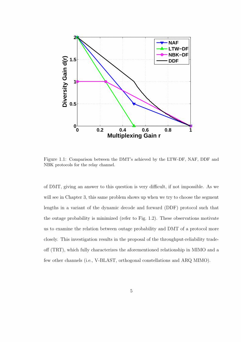
1.1 Comparison between the DMT’s achieved by the LTW-DF, NAF, DDF and
NBK protocols for the relay channel. . . . . . . . . . . . . . . . . . . . . 5
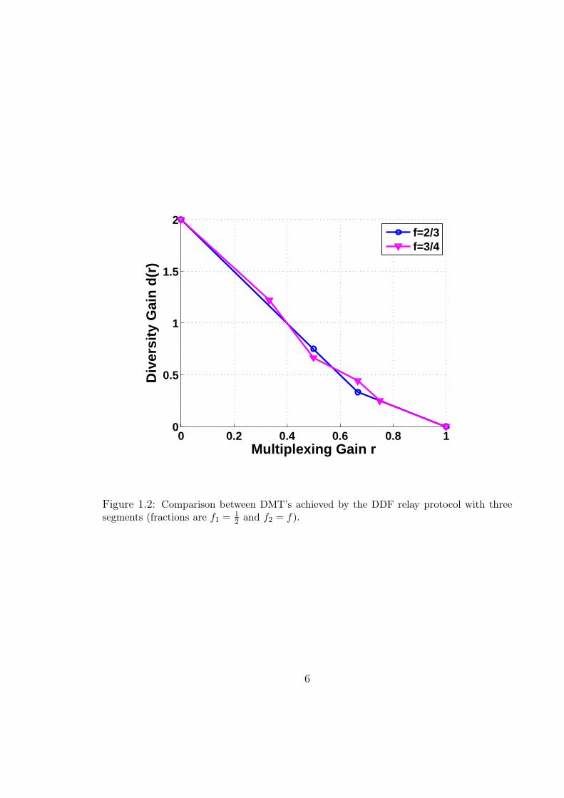
1.2 Comparison between DMT’s achieved by the DDF relay protocol with three
segments (fractions are f1 = 12 and f2 = f). . . . . . . . . . . . . . . . . 6
3.1 The optimal DMT for a single-relay AF protocol. . . . . . . . . . . . . . 18
3.2 The super-frame in the NAF protocol with N − 1 relays. . . . . . . . . . 22
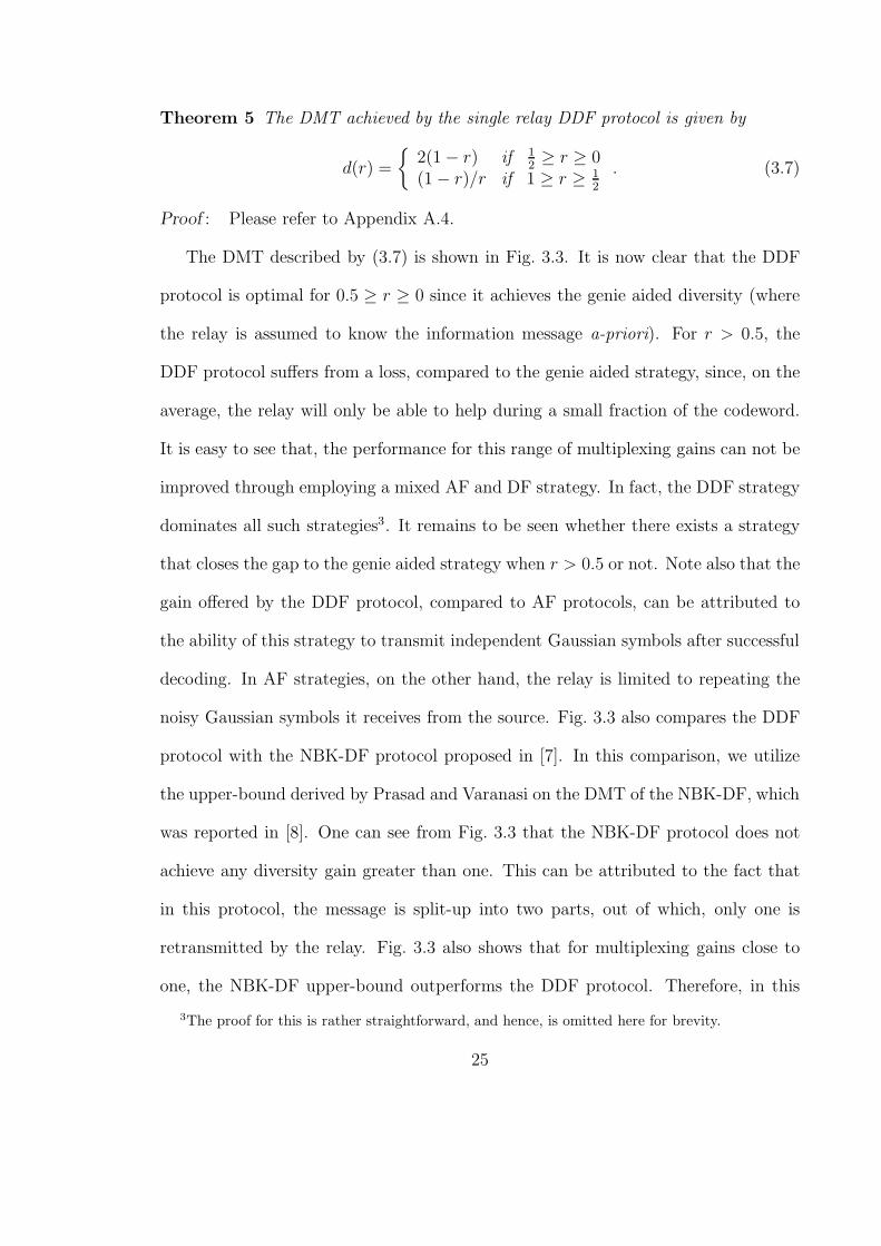
3.3 DMT for the DDF protocol with one relay. . . . . . . . . . . . . . . . . 26
3.4 DMTs achieved by the NAF, DDF, LW-STC, and genie aided protocols with
4 relays. . . . . . . . . . . . . . . . . . . . . . . . . . . . . . . . . . . 28
3.5 DMTs achieved by the DDF protocol with different number of relays. . . . 29
3.6 DMTs achieved by the Pareto optimal DDF protocols with N = 1, 2 and ∞. 33
3.7 Comparison of the outage probability for the NAF, LTW-AF, and non-
cooperative 1 × 1 protocols. . . . . . . . . . . . . . . . . . . . . . . . . 35
3.8 Comparison of the outage probability for the DDF, LTW-AF and non-
cooperative 1 × 1 protocols. . . . . . . . . . . . . . . . . . . . . . . . . 36
4.1 The DMT achieved by the DDF protocol in the MAR channel, along with
an upper-bound on the achievable DMT . . . . . . . . . . . . . . . . . . 41
4.2 The cooperation frame, super-frame and coherence-interval in the CMA-
NAF protocol with N sources. . . . . . . . . . . . . . . . . . . . . . . . 43
xii
4.3 Comparison of the outage probability for the CMA-NAF, LTW-AF and
genie-aided 2 × 1 protocols (N = 2). . . . . . . . . . . . . . . . . . . . . 48
5.1 The DMTachieved by the ARQ-DDF protocol in the CVMA channel, along
with an upper-bound on the achievable DMT (L = 2). . . . . . . . . . . . 54
6.1 Outage curves corresponding to R = 4, 8 BPCU, for a 2 × 2 MIMO channel. 58
6.2 Outage curves corresponding to R = 28, 32 BPCU, for a 2× 2 MIMO channel. 59
6.3 The notion of multiplexing gain restricts the scenarios of interest to those
in which R asymptotically scales linearly with log ρ, i.e. R ∼ r log ρ. . . . . 61
6.4 Relaxing the constraint imposed by the multiplexing gain notion; A multi-
plexing gain cannot be defined for the depicted trajectory, however, since
it remains well within an operating region (i.e. R(1)) TRT analysis can be
applied. . . . . . . . . . . . . . . . . . . . . . . . . . . . . . . . . . . 62
6.5 The constant rate trajectory with R = 20 BPCU passes through different
operating regions in a 2 × 2 MIMO system . . . . . . . . . . . . . . . . . 69
6.6 Outage curves corresponding to R = 20 BPCU for a 2 × 2 MIMO channel.
The solid segment corresponds to the R(1) operating region. . . . . . . . 70
6.7 Outage curves corresponding to R = 20, 24 BPCU for a 2×2 MIMO channel.
The solid segments correspond to the R(1) operating region. . . . . . . . 71
6.8 Outage curves corresponding to R = 4, 10 BPCU for a 3×3 MIMO channel.
The solid segments correspond to the R(1) operating region. . . . . . . . 72
6.9 Outage curves corresponding to R = 58, 64 BPCU for a 3×3 MIMO channel.
The solid segments correspond to the R(2) operating region. . . . . . . . 73
6.10 Outage curves corresponding to R = 40 BPCU for a 3 × 3 MIMO channel.
The solid segment corresponds to the R(2) operating region. . . . . . . . 74
6.11 Outage curves corresponding to R = 34, 40 BPCU for a 3×3 MIMO channel.
The solid segments correspond to the R(2) operating region. . . . . . . . 75
xiii
6.12 Outage probability curves for the 2×2 MIMO channel (dashed), along with
the piecewise-linear approximation (solid) suggested by TRT. . . . . . . . 76
6.13 Outage probability curves for the 3×3 MIMO channel (dashed), along with
the piecewise-linear approximation (solid) suggested by TRT. . . . . . . . 77
6.14 Outage curves corresponding to R = 8, 12 BPCU for a 2×2 V-BLAST scheme. 80
6.15 Comparison of outage curves corresponding to R = 4, 16, 32 BPCU for the
2 × 2 MIMO channel and the V-BLAST scheme. . . . . . . . . . . . . . 81
6.16 Outage curves corresponding to R = 4, 8 BPCU for the 2×2 Alamouti scheme. 84
6.17 Comparison of outage curves corresponding to R = 4, 16, 32 BPCU for the
2 × 2 MIMO channel and the Alamouti scheme. . . . . . . . . . . . . . . 85
A.1 Outage Region for the NAF protocol with a single relay. . . . . . . . . . 101
A.2 Outage Region for the DDF protocol with a single relay (f ≤ 0.5). . . . . 106
A.3 Outage Region for the DDF protocol with a single relay (f > 0.5). . . . . 107
xiv
CHAPTER 1
INTRODUCTION
1.1 Motivation
Recently, there has been a growing interest in the design and analysis of co-
operative transmission protocols [1]-[16]. This is partly due to the ever-increasing
popularity of potential applications such as cellular communications, wireless LANs
and ad-hoc networks, and partly due to the attainable performance gains in terms of
improved throughput, reliability and energy-efficiency. While user cooperation finds
applications in a rather wide range of scenarios (e.g., fading vs. AWGN, ergodic
vs. quasi-static and full-duplex vs. half-duplex), the basic idea is invariably that
users, through pooling together their transmission resources such as power and an-
tennas, can achieve a better performance compared to the case when they operate
individually.
The term cooperative diversity appeared first in the work by Sendonaris, Erkip
and Aazhang [1, 2]. In this work, a multiple-access (MA) scenario was considered
where each user, through employing spreading codes, had been devoted a number
of orthogonal sub-channels. As a result of orthogonality, a user’s signal could be
received at the end of the sub-channel, without interference from other users. Each
1
user then devoted one of its sub-channels for communication to the destination, and
the rest for communication with the other users. This way, users could transmit their
own messages and at the same time help others by relaying (an estimation of) their
messages. The performance of this protocol was analyzed in terms of achievable rate-
region and outage probability. Although this work takes the credit for introducing
the concept of cooperative diversity, the proposed protocol suffered from unnecessary
complications induced by the spreading codes, which in turn made the analysis not
very straightforward. Also, some of the assumptions made, such as availability of
channel state information (CSI) at the users, or, users being able to simultaneously
transmit and receive (i.e. full-duplex communication), were not very practical.
The next and maybe the most influential work in the context of cooperative com-
munications was the one by Laneman, Tse and Wornell [3]. One of the great contri-
butions of this work was to provide a neat system model, which, together with the
intuitive protocols proposed, inspired many people for conducting follow-on research
(e.g., [5, 6]). Laneman et al., too, considered a (two-user) MA scenario, however, they
restricted the users to be half-duplex (i.e., no simultaneous transmission and reception
was allowed). Furthermore, they adopted a coherent communication model, meaning
that CSI was not available to the users. In this work, too, the channel was divided into
(two) orthogonal sub-channels, however instead of using spreading codes, a Time Di-
vision Multiple Access (TDMA) framework was used. This made both understanding
and analyzing of protocols much easier. The basic idea behind the protocols proposed
in this work was to leverage the antenna available at the other user as a source of vir-
tual spatial diversity. The proposed protocols were broadly classified as either amplify
and forward (LTW-AF), where the helping node retransmitted a scaled version of its
2
soft observation, or decode and forward (LTW-DF), where the helping node decoded
the information stream before repeating it. It was shown in [3] that the LTW-AF pro-
tocol achieved full-diversity gain (i.e., two levels of diversity for two users). However,
the LTW-DF protocol failed in achieving a diversity gain greater than one. This, as
was shown later, was a consequence of not encoding the information stream, rather
than the protocol itself; In [4], Laneman and Wornell generalized the LTW-DF pro-
tocol into arbitrary number of users (LW-STC). Furthermore, they used a space-time
code, originally designed for a multiple-input multiple-output (MIMO) channel, to
encode the information stream in a distributed fashion. They then showed that the
LW-STC protocol (and therefore the coded version of LTW-DF protocol) achieved
full cooperative diversity, in the number of cooperating users.
Other follow-on works mainly focused on incorporation of various types of channel
codes (i.e., outer codes such as convolutional and turbo codes), into the LTW-DF
protocol in an attempt to exploit the promised information-theoretic gains (e.g., [5,
6]). It is important to realize that since these protocols use LTW-DF protocol’s
underlying signalling (i.e., inner code), from an information-theoretic point of view,
they are not new protocols.
It was observed by Laneman et. al., that the protocols proposed in [3, 4] (and
subsequently the follow-on works) suffered from a significant loss of performance in the
high spectral efficiency scenario. In fact, the authors of [3] posed the following open
problem: “a key area of further research is exploring cooperative diversity protocols
in the high spectral efficiency regime.” This remark motivates our work here, where
we present efficient (and in many cases optimal) AF and DF protocols for the relay,
3
cooperative broadcast (CB), multiple-access relay (MAR) and cooperative multiple-
access (CMA) channels, along with their automatic repeat request (ARQ) variants.
Another difficulty in the area of (cooperation) protocol design is that, except for
the simplest protocols, traditional performance evaluation techniques such as bit-
error-rate and outage probability analysis, become mathematically intractable. To
get around this problem, we adopt the diversity-multiplexing tradeoff (DMT) as our
analysis tool. This powerful tool was introduced by Zheng and Tse for point-to-
point MIMO channels [17] and later used by Tse, Viswanath, and Zheng to study
the (non-cooperative) MA channel [18]. It should be noted, however, that there is
no established relation, in the literature, between the DMT of a protocol and its
fixed-rate outage probability. This may cause difficulties in comparing two protocols’
performances based on their tradeoff curves. As an example, consider the relay pro-
tocol proposed by Nabar, Bolcskei and Kneubuhler (NBK-DF) [7]. In this protocol,
the source splits its message into two parts. It then transmits the first part to the
destination and the relay during the first phase. During the second phase, the source
transmits the second part while the relay retransmits the first part. It is immediate
to realize that since the second part of the message is not being relayed, this protocol
does not achieve a diversity gain greater than one. Yet, the upper-bound on the DMT
achieved by this protocol in the vicinity of r = 11, as characterized by [8], is maximal
among all known protocols (refer to Fig. 1.1). Now, the natural question to ask is
whether there exist any circumstances, under which this maximality (for multiplex-
ing gains close to one) translates into superiority (in terms of outage probability) of
this protocol over protocols that achieve full-diversity. With today’s understanding
1The multiplexing gain r will be defined rigorously in Chapter 2
4
0 0.2 0.4 0.6 0.8 10
0.5
1
1.5
2
Multiplexing Gain r
Div
ersi
ty G
ain
d(r)
NAFLTW−DFNBK−DFDDF
Figure 1.1: Comparison between the DMT’s achieved by the LTW-DF, NAF, DDF andNBK protocols for the relay channel.
of DMT, giving an answer to this question is very difficult, if not impossible. As we
will see in Chapter 3, this same problem shows up when we try to choose the segment
lengths in a variant of the dynamic decode and forward (DDF) protocol such that
the outage probability is minimized (refer to Fig. 1.2). These observations motivate
us to examine the relation between outage probability and DMT of a protocol more
closely. This investigation results in the proposal of the throughput-reliability trade-
off (TRT), which fully characterizes the aforementioned relationship in MIMO and a
few other channels (i.e., V-BLAST, orthogonal constellations and ARQ MIMO).
5
0 0.2 0.4 0.6 0.8 10
0.5
1
1.5
2
Multiplexing Gain r
Div
ersi
ty G
ain
d(r)
f=2/3f=3/4
Figure 1.2: Comparison between DMT’s achieved by the DDF relay protocol with threesegments (fractions are f1 = 1
2 and f2 = f).
6
1.2 Contributions and Outline
In the sequel, we give the dissertation outline and its main contributions.
In Chapter 2, we detail our modeling assumptions and review some of the results
that are extensively used in the rest of the dissertation.
In Chapter 3, we consider the AF and DF relay channels and propose protocols
for each one. The main contributions in this chapter can be summarized as follows.
• For the AF relay channel (single relay), we first establish an upper bound on
the achievable DMT. We then propose a nonorthogonal amplify and forward
(NAF) protocol that achieves this upper bound. Finally, we generalize the NAF
protocol to the case of arbitrary number of relays and characterize its DMT.
Notably, we show that the NAF protocol outperforms the LW-STC protocol
without requiring decoding/encoding at the relays.
• For the DF relay channel (single relay), we propose a dynamic decode and
forward (DDF) protocol and prove its optimality (with respect to DMT), over
the range of multiplexing gains 1/2 ≥ r ≥ 0. Furthermore, we show that the
DDF protocol outperforms all AF protocols at any multiplexing gain. Finally,
we extend the DDF protocol to the case of arbitrary number of relays and
characterize its tradeoff curve.
• We present a novel variant of the (single relay) DDF protocol, which is particu-
larly suitable for implementation. In this variant, the channel seen by the desti-
nation is reduced to a single-input single-output (SISO) time-selective channel.
Furthermore, to reduce the complexity of the protocol, we confine the relay to
start transmission only at the beginning of a finite number of segments. We
7
give the rule for determining these segments such that the variant is Pareto2
optimal with respect to DMT.
In Chapter 4, we propose protocols for the CB, MAR and CMA channels. The
main contributions in this chapter are as follows.
• For the CB channel, we present a variant of the DDF protocol that allows for
efficient transmission of common information. We then establish the superiority
of this protocol, over AF protocols, by characterizing its tradeoff curve. In fact,
it turns out that the gain offered by the DDF protocol is more significant in
this scenario, when compared to the relay channel.
• For the symmetric MAR channel (two users), we first derive an upper bound on
the achievable DMT. We then modify the DDF protocol to match it to the MAR
channel and derive its tradeoff curve. This characterization shows that the DDF
protocol is DMT optimal over the range of multiplexing gains 3/4 ≥ r ≥ 0. It
also reveals that in the MAR channel, a single relay can be utilized by several
users to simultaneously improve the diversity gain achieved by all of them.
• For the symmetric CMA channel, we propose a novel AF protocol where an
artificial inter-symbol interference (ISI) channel is created. We prove the opti-
mality (in terms of DMT) of this protocol by showing that, for all multiplexing
gains (i.e., 1 ≥ r ≥ 0), it achieves the DMT of the corresponding N × 1 MIMO
channel. We then use this result to argue that the sub-optimality of the proto-
cols proposed in [3] is a consequence of using orthogonal sub-channels, rather
2The notion of Pareto optimality will be rigorously defined in Chapter 2.
8
than the half-duplex constraint. We also utilize this result to elucidate the
fundamental difference between the relay and CMA channels.
In Chapter 5, we consider the ARQ relay, MAR and cooperative vector multiple-
access (CVMA) channels and quantify the significant performance gains, attained
through providing the users with a few feedback bits. The main contributions in this
chapter are as follows.
• For the ARQ relay and MAR (two users) channels, we first modify the corre-
sponding DDF protocols (proposed in Chapter 3 and Chapter 4, respectively) to
incorporate ACK/NACK feedback signals. We then characterize their achieved
tradeoff curves, which prove their optimality.
• For the ARQ CVMA channel (two users and two receiving antennas), we develop
a new variant of the DDF protocol where the users are purposefully instructed
not to cooperate in the first round of transmission. Lower and upper bounds
on the achievable DMT are then derived. These bounds are shown to converge
to the optimal tradeoff as the number of transmission rounds increases.
In Chapter 6, we consider an outage limited MIMO channel and build on Zheng
and Tse’s elegant formulation of DMT to develop a better understanding of the
asymptotic relationship between the probability of error, transmission rate, and signal
to noise ratio (SNR). The main contributions in this chapter are summarized in the
following.
• We identify the limitation imposed by the notion of multiplexing gain and de-
velop a new formulation for the throughput-reliability tradeoff that avoids this
9
limitation. In this formulation, the multiplexing gain notion is replaced by the
more general concept of operating regions.
• We use the proposed TRT formulation to elucidate the asymptotic trends ex-
hibited by MIMO channels. In particular, we devise a piecewise linear approx-
imation to the outage probability of MIMO channels (at fixed rates), which
becomes progressively more accurate as rate and SNR grow.
• We characterize the TRT, along with the corresponding piecewise linear outage
approximation, for the V-BLAST, orthogonal constellations and ARQ MIMO
channels.
Finally in Chapter 7, we offer some concluding remarks. To enhance the flow of
the dissertation, we collect all the proofs in the Appendix.
10
CHAPTER 2
BACKGROUND
Throughout the dissertation, we use (x)+ to mean max{x, 0}, (x)− to mean
min{x, 0}, ⌈x⌉ to mean nearest integer to x towards plus infinity and ⌊x⌋ to mean
nearest integer to x towards minus infinity. RN and CN denote the set of real and
complex N -tuples, respectively, while RN+ denotes the set of non-negative N -tuples.
We denote the complement of set O ⊆ RN , in RN , by Oc, while O+ means O ∩ RN+.
IN denotes the N×N identity matrix, Σx denotes the autocovariance matrix of vector
x, and log(.) denotes the base-2 logarithm.
Next, we state the general assumptions that apply to all of the cooperative chan-
nels considered in this dissertation (A separate system model will be given for the
outage-limited MIMO channels considered in Chapter 6). Assumptions pertaining to
a specific scenario will be given in the related Chapter.
• All channels are assumed to be flat Rayleigh-fading and quasi-static, i.e., the
channel gains remain constant during a coherence-interval and change inde-
pendently from one coherence-interval to another. Furthermore, the channel
gains are mutually independent with unit variance. The additive noises at dif-
ferent nodes are zero-mean, mutually-independent, circularly-symmetric and
11
white complex-Gaussian. Furthermore, the variances of these noises are pro-
portional to one another such that there are always fixed offsets between the
different channels’ SNRs.
• All nodes have the same power constraint, operate synchronously and un-
less otherwise stated, have a single antenna (In Section 5.2 we consider the
CVMA scenario where the destination is equipped with two receiving antennas).
Throughout the dissertation, we consider coherent communications meaning
that only the receiving node of any link knows the channel gain. Also, except
for Chapter 5 (where we study ARQ channels), no feedback to the transmitting
node is permitted. Following in the footsteps of [3], all cooperating partners
operate in the half-duplex mode, i.e., at any point in time, a node can either
transmit or receive, but not both. This constraint is motivated by, e.g., the typ-
ically large difference between the incoming and outgoing signal power levels.
• In this work, we exclusively use random Gaussian code-books where a codeword
spans the entire coherence-interval of the channel. Furthermore, we assume
asymptotically large code-lengths, implying that the established DMTs only
serve as upper-bounds on the performance of the protocols that use finite code-
lengths. Results related to the design of practical coding/decoding schemes that
approach the fundamental limits established here are reported in [31].
In the sequel, we summarize several important definitions and results that will be
used throughout the dissertation.
• The SNR of a link, ρ, is defined as
ρ ,E
σ2, (2.1)
12
where E denotes the average energy available for transmission of a symbol across
the link and σ2 denotes the variance of the noise observed at the receiving end
of the link. We say that f(ρ) is exponentially equal to ρb, denoted by f(ρ)=ρb,
when
limρ→∞
log f(ρ)
log ρ= b. (2.2)
In (2.2), b is called the exponential order of f(ρ). ≤ and ≥ are defined similarly.
• Assume that g is a Gaussian random variable with zero mean and unit variance.
If v denotes the exponential order of 1/|g|2, i.e.,
v = − limρ→∞
log |g|2
log ρ, (2.3)
then the probability density function (PDF) of v can be shown to be:
pv = limρ→∞
ln(ρ)ρ−v exp(−ρ−v).
Careful examination of the previous expression reveals that
pv=
{
ρ−∞ = 0, for v < 0,
ρ−v, for v ≥ 0. (2.4)
Thus, for independent random variables {vj}Nj=1 distributed identically to v, the
probability PO that (v1, . . . , vN) belongs to set O can be characterized by
PO=ρ−do where do , inf(v1,...,vN )∈O+
N∑
j=1
vj, (2.5)
provided that O+ is not empty. In other words, the exponential order of PO
only depends on O+. This is due to the fact that the probability of any set,
consisting of N -tuples (v1, . . . , vN) with at least one negative element, decreases
exponentially with SNR and therefore can be neglected compared to PO+ which
decreases polynomially with SNR.
13
• Consider a family of codes {Cρ} indexed by operating SNR ρ, such that the code
Cρ has a rate of R(ρ) bits per channel use (BPCU) and a maximum likelihood
(ML) error probability PE(ρ). For this family, the multiplexing gain r and the
diversity gain d are defined as
r , limρ→∞
R(ρ)
log ρ, d , − lim
ρ→∞
logPE(ρ)
log ρ. (2.6)
• The problem of characterizing the optimal tradeoff between the reliability and
throughput of a point-to-point communication system over a coherent quasi-
static flat Rayleigh-fading channel was posed and solved by Zheng and Tse
in [17]. For a MIMO communication system with M transmit and N receive
antennas, they showed that, for any min{M,N} ≥ r ≥ 0, the optimal diver-
sity gain d∗(r) is given by the piecewise linear function joining the (r, d) pairs
(k, (M − k)(N − k)) for k = 0, ...,min{M,N}, provided that the code-length l
satisfies l ≥M +N − 1.
• We say that protocol A is uniformly optimal, if for every protocol B, dA(r) ≥
dB(r), ∀r.
• We say that protocol A is Pareto optimal, if there is no protocol B dominating
protocol A in the Pareto sense. Protocol B is said to dominate protocol A in
the Pareto sense if there is some r0 for which dB(r0) > dA(r0), but no r such
that dB(r) < dA(r).
• Consider a coherent linear Gaussian channel, i.e.
y = s + n,
14
where, s ∈ CN and n ∈ C
N denote the signal and noise components of the
observed vector, respectively. For this channel, the pairwise error probability
(PEP) of the ML decoder, denoted by PPE, averaged over the ensemble of
random Gaussian codes, is upper bounded by
PPE ≤ det(IN +1
2ΣsΣ
−1n )−1. (2.7)
• The following lemma will be used in characterizing the DMT of DDF protocols.
Lemma 1 Consider a coherent linear Gaussian channel of data rate R and
codeword length l. The error probability of the ML decoder utilizing a frac-
tion of the code-word such that the mutual information between the received and
transmitted signals exceeds lR, averaged over the ensemble of random Gaus-
sian codes, can be made arbitrarily small provided that the codeword length l is
sufficiently large.
Proof : Please refer to Appendix A.1.
15
CHAPTER 3
RELAY CHANNEL
In this chapter, we consider the relay channel, where N − 1 relays help a single
source to better transmit its message to the destination. As the vague descriptions
help and better transmit suggest, the general relay problem is rather broad and only
certain sub-problems have been studied (for example see [24]). In this chapter, we
focus on two important classes of relay protocols. The first is the class of amplify and
forward (AF) protocols, where a relaying node can only process the observed signal
linearly before re-transmitting it. The second is the class of decode and forward (DF)
protocols, where the relays are allowed to decode and re-encode the message using (a
possibly different) code-book. Here we emphasize that, a priori, it is not clear which
class (i.e., AF or DF) offers a better performance (e.g., [3]).
3.1 Amplify and Forward Protocols
We first consider the single relay scenario (i.e., N = 2). For this scenario, we
derive the optimal DMT and identify a specific protocol within this class, i.e., the
NAF protocol that achieves this optimal tradeoff. We then extend the NAF protocol
to the general case with an arbitrary number of relays.
16
Under the half-duplex constraint, it is easy to see that any single-relay AF protocol
can be mathematically described by some choice of the matrices A1, A2, and B in
the following model
y =
[g1A1 0
g2hBA1 g1A2
]
x +
[0g2B
]
w + v. (3.1)
In (3.1), y ∈ Cl represents the vector of observations at the destination, x ∈ Cl the
vector of source symbols, w ∈ Cl′ the vector of noise samples (of variance σ2w) observed
by the relay, and v ∈ Cl the vector of noise samples (of variance σ2
v) observed by the
destination. The variables h, g1 and g2 denote the source-relay channel gain, source-
destination channel gain, and relay-destination channel gain, respectively. A1 ∈ Cl′×l′
and A2 ∈ C(l−l′)×(l−l′) are diagonal matrices. In this protocol, the source can poten-
tially transmit a new symbol in every symbol-interval of the codeword, while the relay
listens during the first l′ symbols and then, for the remaining l− l′ symbols, transmits
linear combinations of the l′ noisy observations using the coefficients in B ∈ C(l−l′)×l′ .
In fact, by letting l′ = l/2, A1 = Il′, A2 = 0 and B = bIl′ (with b ≤√
E/(|h|2E + σ2w)
denoting the relay repetition gain), we obtain the LTW-AF protocol [3]. Finally, we
note that when the source symbols are independent, the average energy constraint
translates to
|h|2El′∑
i=1
|bji|2|ai|
2 + σ2w
l′∑
i=1
|bji|2 ≤ E, j = 1, . . . , l − l′, (3.2)
where B = [bji] and A1 = diag(a1, · · · , al′).
Theorem 2 The optimal diversity gain for the relay channel with a single AF relay
is upper-bounded by
d∗(r) ≤ (1 − r) + (1 − 2r)+. (3.3)
17
0 0.2 0.4 0.6 0.8 10
0.2
0.4
0.6
0.8
1
1.2
1.4
1.6
1.8
2
Multiplexing Gain r
Div
ersi
ty G
ain
d(r)
The Non−cooperative StrategyThe NAF StrategyThe LTW−AF Strategy
Figure 3.1: The optimal DMT for a single-relay AF protocol.
18
Proof : Please refer to Appendix A.2.
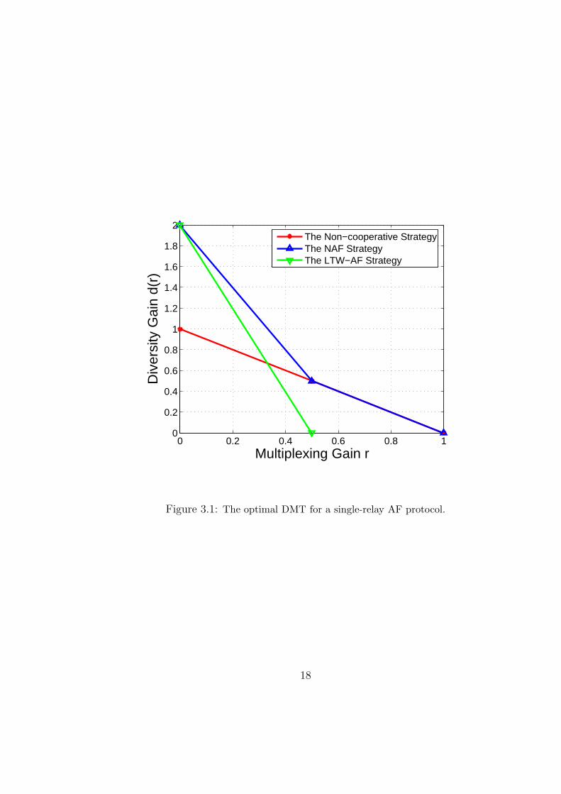
The upper-bound on d∗(r), as given by (3.3), is shown in Fig. 3.1. Having Theorem
2 at hand, it now suffices to identify an AF protocol that achieves this upper-bound
in order to establish its optimality. Towards this end, we observe that, in the proof of
Theorem 2, the only requirements onB such that the protocol described by (3.1) could
potentially achieve the optimal DMT are that B is square (of dimension l/2 × l/2)
and full-rank. Furthermore, B should not violate the relay average energy constraint
as given by (3.2). Thus, the simple choices
A1 = Il/2 A2 = Il/2 B = bIl/2 for b ≤
√
E
|h|2E + σ2w
(3.4)
inspire the NAF protocol. In particular, the source transmits on every symbol-interval
in a cooperation frame, where a cooperation frame is defined as two consecutive
symbol-intervals. The relay, on the other hand, transmits only once per cooperation
frame; it simply repeats the (noisy) signal it observed during the previous symbol-
interval. It is important to realize that this design is dictated by the half-duplex
constraint, which implies that the relay can repeat at most once per cooperation
frame. We denote the repetition gain by b and, for frame k, we denote the information
symbols by {xj,k}2j=1. The signals received by the destination during frame k are thus:
y1,k = g1x1,k + v1,k
y2,k = g1x2,k + g2b(hx1,k + w1,k) + v2,k
where the repetition gain b satisfies (3.4). Note that, in order to decode the message,
the destination needs to know the relay repetition gain b, the source-relay channel
gain h, the source-destination channel gain g1, and the relay-destination channel gain
19
g2. Now, we are ready to establish the optimality of the NAF protocol with respect
to DMT.
Theorem 3 The NAF protocol achieves the optimal DMT of the AF single-relay
scenario, which is
d∗(r) = (1 − r) + (1 − 2r)+. (3.5)
Proof : Please refer to Appendix A.3.
Three remarks are now in order:
1. As shown in Fig. 3.1, the NAF protocol enjoys uniform dominance over the
direct transmission scheme (i.e., no cooperation) and LTW-AF protocol. This
dominance can be attributed to relaxing the orthogonality constraint whereby
one can reap two distinct benefits: rate enhancement via continuous transmis-
sion and diversity enhancement via cooperation. It is interesting to note that
this dominance is achieved while only half of the symbols are repeated by the
relay.
2. From Fig. 3.1, one can see that for multiplexing gains greater that 0.5, the
diversity gain achieved by the NAF relay protocol is identical to that of the
non-cooperative protocol. This is due to the fact that the AF cooperative link
provided by the relay can not support multiplexing gains greater than 0.5–a
consequence of the half-duplex constraint. Hence, for multiplexing gains larger
than 0.5, there is only one link from the source to the destination, and thus, the
tradeoff curve is identical to that of a point-to-point system with one transmit
and one receive antenna. Later, we will show that the proposed DDF strategy
avoids this drawback.
20
3. As shown in the proof of Theorem 3, the achievability of the optimal tradeoff is
not very sensitive to the choice of the repetition gain “b” (i.e., for a wide range
of choices, the NAF protocol achieves the optimal tradeoff). In practice, one
should optimize the repetition gain, experimentally if needed, to minimize the
outage probability at the target rate and SNR.
The NAF protocol can be extended to the case of arbitrary number of relays (i.e., N ≥
2) as follows. First, we define a super-frame as a concatenation of N − 1 consecutive
cooperation frames. Within each super-frame, the relays take turns repeating the
signals they previously observed as they did in the case of a single relay (refer to
Fig. 3.2). Thus, the destination’s received signals during a super-frame will be
y1,1 = g1x1,1 + v1,1
y2,1 = g1x2,1 + g2b2(h2x1,1 + w1,1) + v2,1
y1,2 = g1x1,2 + v1,2
y2,2 = g1x2,2 + g3b3(h3x1,2 + w1,2) + v2,2
...
y1,N−1 = g1x1,N−1 + v1,N−1
y2,N−1 = g1x2,N−1 + gNbN (hNx1,N−1 + w1,N−1) + v2,N−1,
where the source-relay channel gain, relay-destination channel gain, relay repetition
gain, and relay-observed noise for relay i ∈ {1, ..., N − 1} are denoted by hi+1, gi+1,
bi+1 and w1,i, respectively. As before, g1 represents the source-destination channel
gain. The quantities yj,k, vj,k, and xj,k represent the received signal, noise sample,
and source symbol, respectively, during the jth symbol-interval of the kth coopera-
tion frame. Note that there is nothing to be gained by having more than one relay
21
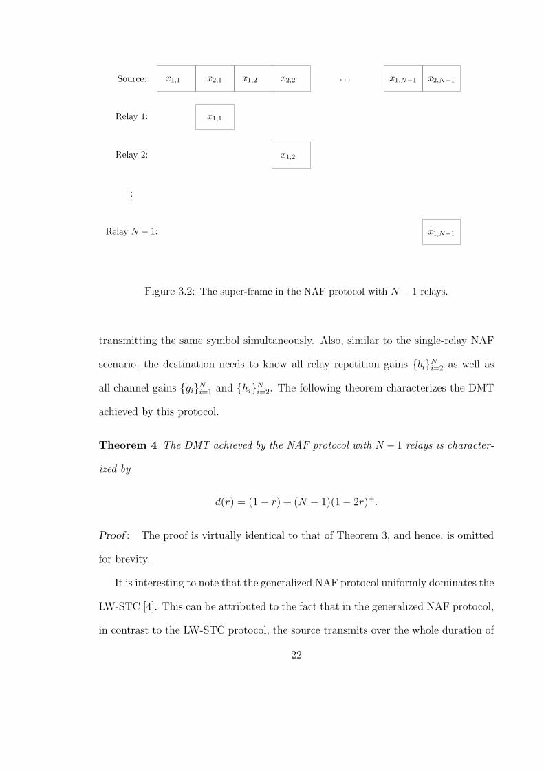
Source:
x1,1
x1,1 x2,1
x1,2
x1,2 x2,2 · · ·
x1,N−1
x1,N−1 x2,N−1
Relay 1:
Relay 2:
...
Relay N − 1:
Figure 3.2: The super-frame in the NAF protocol with N − 1 relays.
transmitting the same symbol simultaneously. Also, similar to the single-relay NAF
scenario, the destination needs to know all relay repetition gains {bi}Ni=2 as well as
all channel gains {gi}Ni=1 and {hi}
Ni=2. The following theorem characterizes the DMT
achieved by this protocol.
Theorem 4 The DMT achieved by the NAF protocol with N − 1 relays is character-
ized by
d(r) = (1 − r) + (N − 1)(1 − 2r)+.
Proof : The proof is virtually identical to that of Theorem 3, and hence, is omitted
for brevity.
It is interesting to note that the generalized NAF protocol uniformly dominates the
LW-STC [4]. This can be attributed to the fact that in the generalized NAF protocol,
in contrast to the LW-STC protocol, the source transmits over the whole duration of
22
the codeword. The generalized NAF protocol offers the additional advantage of low
complexity since it does not require decoding/encoding at the relays.
3.2 Decode and Forward Protocols
In this class of protocols, we allow for the possibility of decoding/encoding at the
different relays. In [3], Laneman-Tse-Wornell presented a particular variant of DF
protocols (LTW-DF) where the source transmits in the first half of the codeword.
Based on its received signal in this interval, the relay attempts to decode the mes-
sage. It then re-encodes and transmits the encoded stream in the second half of the
codeword. In [4], Laneman and Wornell derived the DMT achieved by this scheme
(i.e., d(r) = 2(1 − 2r)), which is depicted in Fig. 3.3. Here, we propose a dynamic
decode and forward (DDF) protocol and characterize its tradeoff curve. This charac-
terization reveals the uniform dominance of this protocol over all known full-diversity
(i.e., d(0) = 2) protocols proposed for the half-duplex single-relay channel and fur-
thermore establishes its optimality, over a certain range of multiplexing gains (i.e.,
1/2 ≥ r ≥ 0). We first describe and analyze the protocol for the case of a single relay.
Generalization to N − 1 relays will then follow.
We assume that a codeword consists of l consecutive symbol-intervals, during
which all the channel gains remain unchanged. In the DDF protocol, the source
transmits data at a rate of R BPCU during every symbol-interval in the codeword.
The relay, on the other hand, listens to the source until the mutual information be-
tween its received signal and source signal exceeds lR. It then decodes and re-encodes
the message using an independent Gaussian code-book and transmits it during the
rest of the codeword. The dynamic nature of the protocol is manifested in the fact
23
that we allow the relay to listen for a time duration that depends on the instanta-
neous channel realization to maximize the probability of successful decoding. We
denote the signals transmitted by the source and relay as {xk}lk=1 and {xk}
lk=l′+1,
respectively, where l′ is the number of symbol-intervals the relay waits before starting
transmission. Using this notation, the received signals (at the destination) can be
written as:
yk =
{g1xk + vk for l′ ≥ k ≥ 1g1xk + g2xk + vk for l ≥ k > l′
.
From the protocol description, it is clear that the number of symbols where the relay
listens should be chosen as:
l′ = min
{
l,
⌈lR
log (1 + |h|2cρ)
⌉}
, (3.6)
where h is the source-relay channel gain, and c = σ2v/σ
2w. One can now see the
dependence of this choice of l′ on the instantaneous channel realization and that
this choice, together with the asymptotically large l, guarantees that when l′ < l,
the relay average probability of error with a Gaussian code ensemble is arbitrarily
small (recall Lemma 1). Clearly, when l′ = l the relay does not contribute to the
transmission of the message, and hence, incorrect decoding at the relay in this case
does not affect performance. Here, we observe that, in contrast to the NAF protocol,
the destination does not need to know the source-relay channel gain. It does, however,
need to know the relay waiting time l′, along with the source-destination and relay-
destination channel gains. The following theorem describes the DMT achievable with
this cooperation protocol.
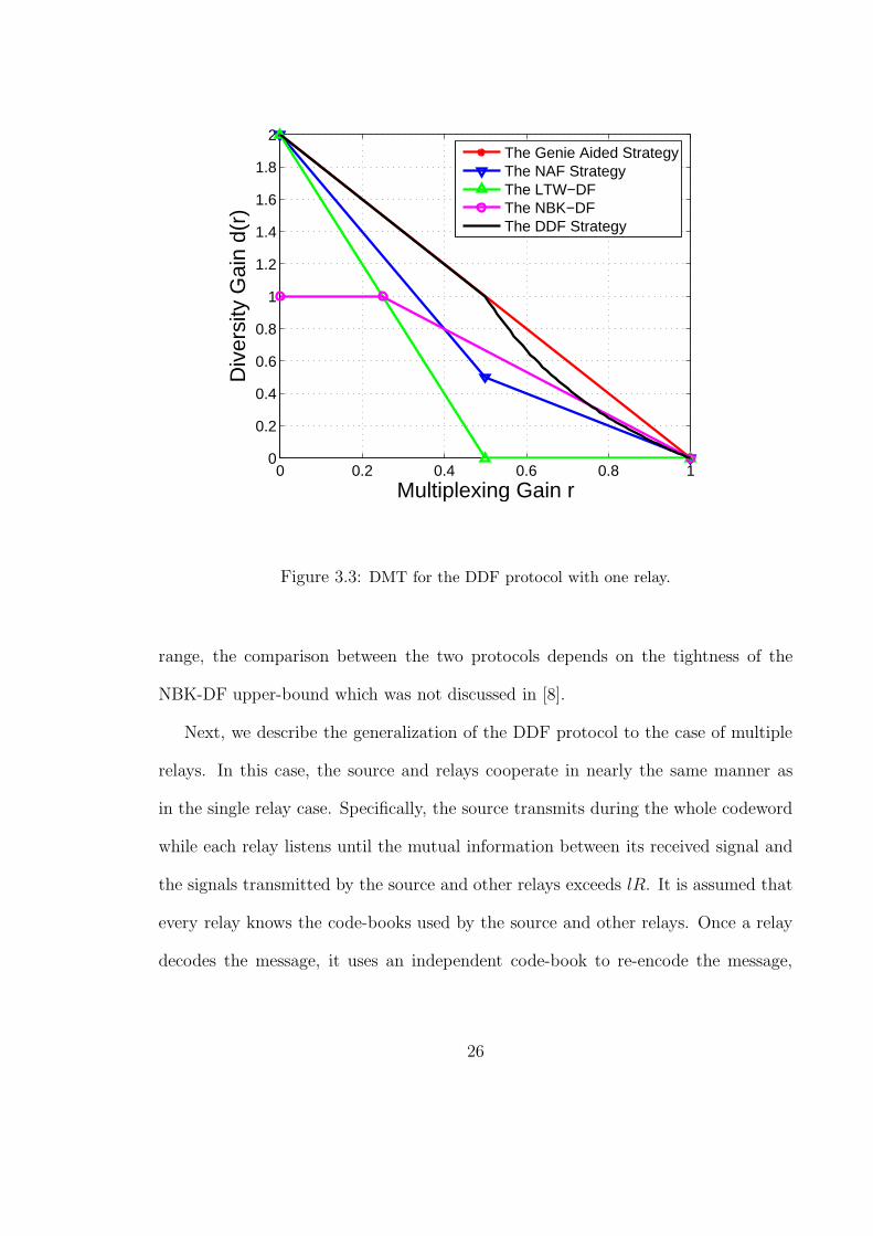
24
Theorem 5 The DMT achieved by the single relay DDF protocol is given by
d(r) =
{2(1 − r) if 1
2≥ r ≥ 0
(1 − r)/r if 1 ≥ r ≥ 12
. (3.7)
Proof : Please refer to Appendix A.4.
The DMT described by (3.7) is shown in Fig. 3.3. It is now clear that the DDF
protocol is optimal for 0.5 ≥ r ≥ 0 since it achieves the genie aided diversity (where
the relay is assumed to know the information message a-priori). For r > 0.5, the
DDF protocol suffers from a loss, compared to the genie aided strategy, since, on the
average, the relay will only be able to help during a small fraction of the codeword.
It is easy to see that, the performance for this range of multiplexing gains can not be
improved through employing a mixed AF and DF strategy. In fact, the DDF strategy
dominates all such strategies3. It remains to be seen whether there exists a strategy
that closes the gap to the genie aided strategy when r > 0.5 or not. Note also that the
gain offered by the DDF protocol, compared to AF protocols, can be attributed to
the ability of this strategy to transmit independent Gaussian symbols after successful
decoding. In AF strategies, on the other hand, the relay is limited to repeating the
noisy Gaussian symbols it receives from the source. Fig. 3.3 also compares the DDF
protocol with the NBK-DF protocol proposed in [7]. In this comparison, we utilize
the upper-bound derived by Prasad and Varanasi on the DMT of the NBK-DF, which
was reported in [8]. One can see from Fig. 3.3 that the NBK-DF protocol does not
achieve any diversity gain greater than one. This can be attributed to the fact that
in this protocol, the message is split-up into two parts, out of which, only one is
retransmitted by the relay. Fig. 3.3 also shows that for multiplexing gains close to
one, the NBK-DF upper-bound outperforms the DDF protocol. Therefore, in this
3The proof for this is rather straightforward, and hence, is omitted here for brevity.
25
0 0.2 0.4 0.6 0.8 10
0.2
0.4
0.6
0.8
1
1.2
1.4
1.6
1.8
2
Multiplexing Gain r
Div
ersi
ty G
ain
d(r)
The Genie Aided StrategyThe NAF StrategyThe LTW−DFThe NBK−DFThe DDF Strategy
Figure 3.3: DMT for the DDF protocol with one relay.
range, the comparison between the two protocols depends on the tightness of the
NBK-DF upper-bound which was not discussed in [8].
Next, we describe the generalization of the DDF protocol to the case of multiple
relays. In this case, the source and relays cooperate in nearly the same manner as
in the single relay case. Specifically, the source transmits during the whole codeword
while each relay listens until the mutual information between its received signal and
the signals transmitted by the source and other relays exceeds lR. It is assumed that
every relay knows the code-books used by the source and other relays. Once a relay
decodes the message, it uses an independent code-book to re-encode the message,
26
which it then transmits for the rest of the codeword. Note that, since the source-
relay channel gains may differ, the relays may require different waiting times for
decoding. This complicates the protocol, since a given relay’s ability to decode the
message requires precise knowledge of the times at which every other relay begins
its transmission. To address this problem, the codeword is divided into a number
of segments, and relays are allowed to start transmission only at the beginning of
a segment. In between the segments, every relay is allowed to broadcast a (well
protected) beacon, informing all other relays whether or not it will start transmission.
Judicious choice of the segment length, relative to the codeword length, results in only
a small loss compared to the genie-aided case, whereby all relays know all decoding
times a-priori. Here, we assume that the number of segments is sufficiently large and
the length of the beacon signals is much smaller than the segment length. Therefore,
in characterizing the DMT achieved by this protocol, we ignore the losses associated
with the beacons and the quantization of the starting times for the different relays.
Theorem 6 The DMT achieved by the DDF protocol with N −1 relays is character-
ized by:
d(r) =
N(1 − r), 1N
≥ r ≥ 0,
1 + (N−1)(1−2r)1−r
, 12≥ r ≥ 1
N,
1−rr, 1 ≥ r ≥ 1
2.
(3.8)
Proof : Please refer to Appendix A.5.
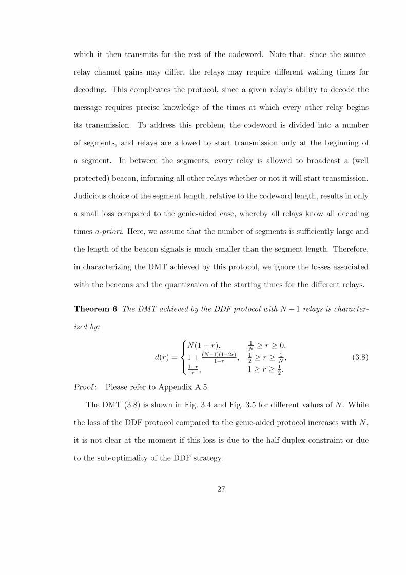
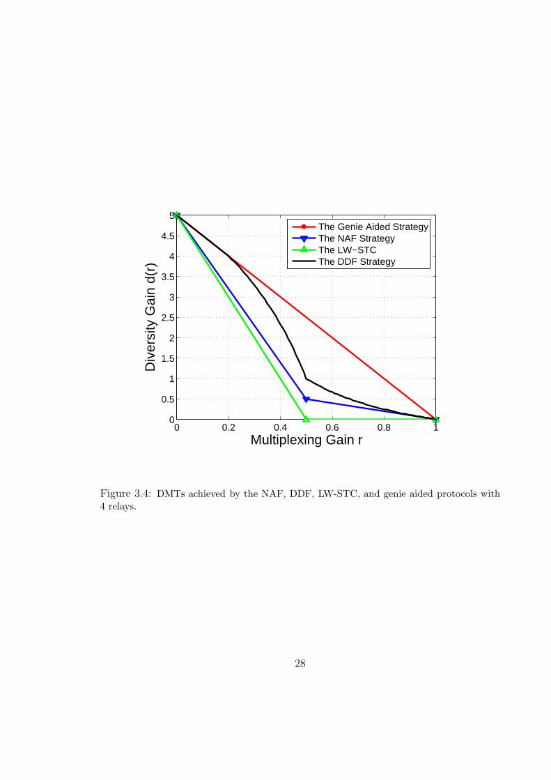
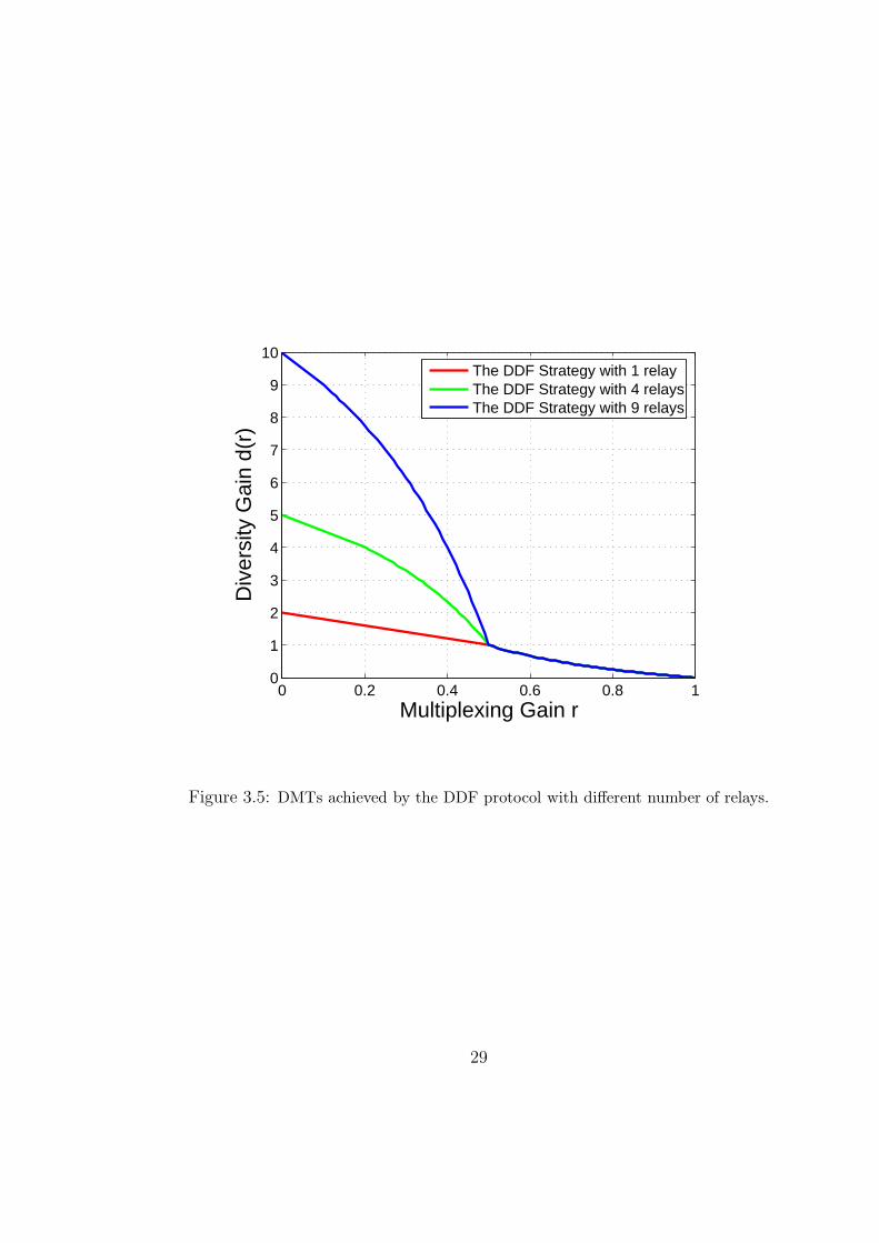
The DMT (3.8) is shown in Fig. 3.4 and Fig. 3.5 for different values of N . While
the loss of the DDF protocol compared to the genie-aided protocol increases with N ,
it is not clear at the moment if this loss is due to the half-duplex constraint or due
to the sub-optimality of the DDF strategy.
27
0 0.2 0.4 0.6 0.8 10
0.5
1
1.5
2
2.5
3
3.5
4
4.5
5
Multiplexing Gain r
Div
ersi
ty G
ain
d(r)
The Genie Aided StrategyThe NAF StrategyThe LW−STCThe DDF Strategy
Figure 3.4: DMTs achieved by the NAF, DDF, LW-STC, and genie aided protocols with4 relays.
28
0 0.2 0.4 0.6 0.8 10
1
2
3
4
5
6
7
8
9
10
Multiplexing Gain r
Div
ersi
ty G
ain
d(r)
The DDF Strategy with 1 relayThe DDF Strategy with 4 relaysThe DDF Strategy with 9 relays
Figure 3.5: DMTs achieved by the DDF protocol with different number of relays.
29
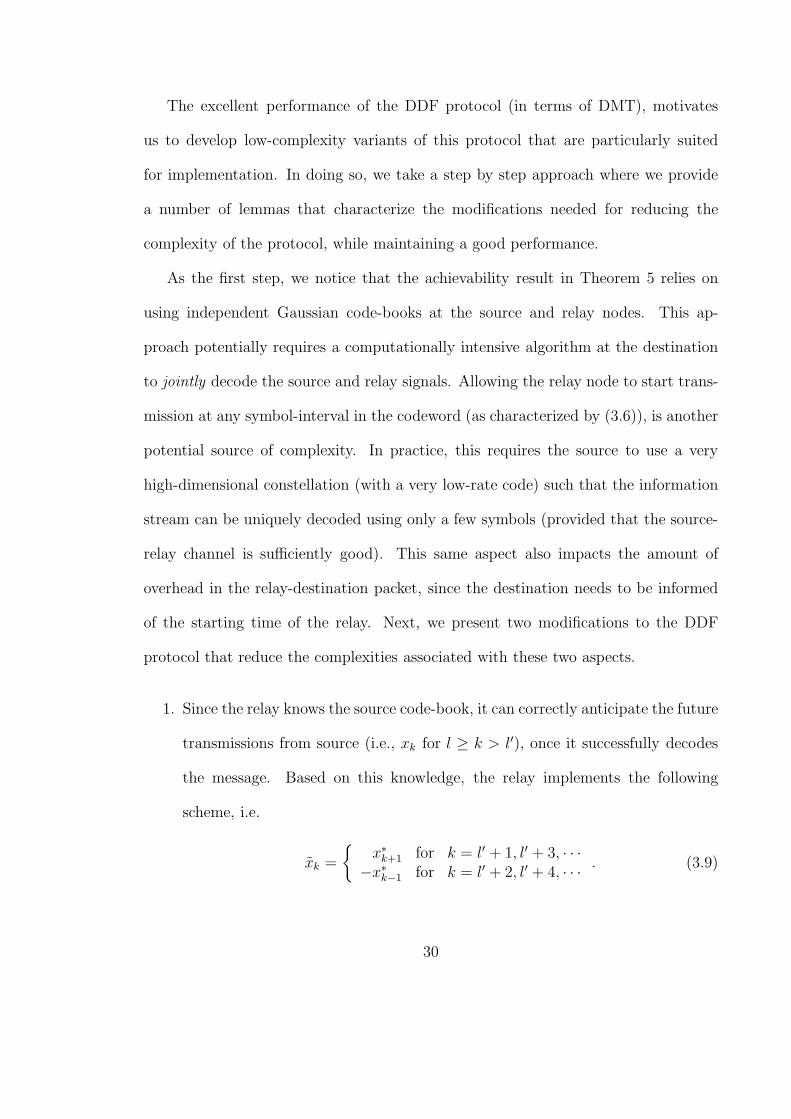
The excellent performance of the DDF protocol (in terms of DMT), motivates
us to develop low-complexity variants of this protocol that are particularly suited
for implementation. In doing so, we take a step by step approach where we provide
a number of lemmas that characterize the modifications needed for reducing the
complexity of the protocol, while maintaining a good performance.
As the first step, we notice that the achievability result in Theorem 5 relies on
using independent Gaussian code-books at the source and relay nodes. This ap-
proach potentially requires a computationally intensive algorithm at the destination
to jointly decode the source and relay signals. Allowing the relay node to start trans-
mission at any symbol-interval in the codeword (as characterized by (3.6)), is another
potential source of complexity. In practice, this requires the source to use a very
high-dimensional constellation (with a very low-rate code) such that the information
stream can be uniquely decoded using only a few symbols (provided that the source-
relay channel is sufficiently good). This same aspect also impacts the amount of
overhead in the relay-destination packet, since the destination needs to be informed
of the starting time of the relay. Next, we present two modifications to the DDF
protocol that reduce the complexities associated with these two aspects.
1. Since the relay knows the source code-book, it can correctly anticipate the future
transmissions from source (i.e., xk for l ≥ k > l′), once it successfully decodes
the message. Based on this knowledge, the relay implements the following
scheme, i.e.
xk =
{x∗k+1 for k = l′ + 1, l′ + 3, · · ·
−x∗k−1 for k = l′ + 2, l′ + 4, · · ·. (3.9)
30
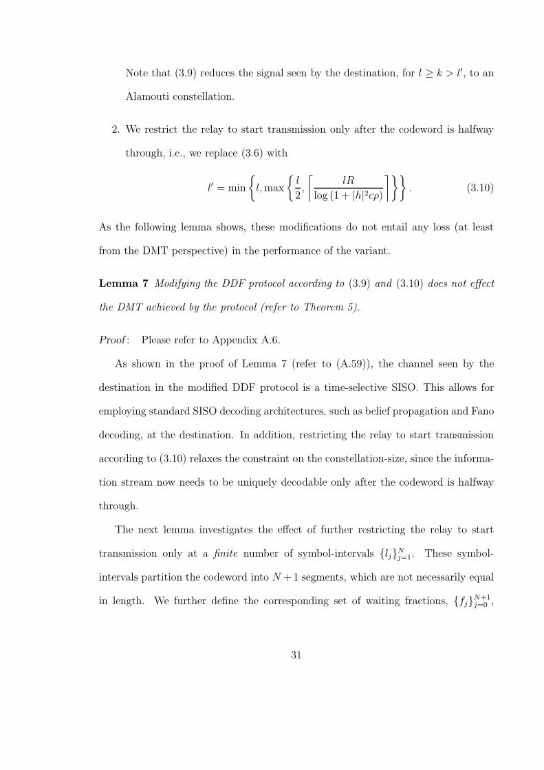
Note that (3.9) reduces the signal seen by the destination, for l ≥ k > l′, to an
Alamouti constellation.
2. We restrict the relay to start transmission only after the codeword is halfway
through, i.e., we replace (3.6) with
l′ = min
{
l,max
{l
2,
⌈lR
log (1 + |h|2cρ)
⌉}}
. (3.10)
As the following lemma shows, these modifications do not entail any loss (at least
from the DMT perspective) in the performance of the variant.
Lemma 7 Modifying the DDF protocol according to (3.9) and (3.10) does not effect
the DMT achieved by the protocol (refer to Theorem 5).
Proof : Please refer to Appendix A.6.
As shown in the proof of Lemma 7 (refer to (A.59)), the channel seen by the
destination in the modified DDF protocol is a time-selective SISO. This allows for
employing standard SISO decoding architectures, such as belief propagation and Fano
decoding, at the destination. In addition, restricting the relay to start transmission
according to (3.10) relaxes the constraint on the constellation-size, since the informa-
tion stream now needs to be uniquely decodable only after the codeword is halfway
through.
The next lemma investigates the effect of further restricting the relay to start
transmission only at a finite number of symbol-intervals {lj}Nj=1. These symbol-
intervals partition the codeword into N +1 segments, which are not necessarily equal
in length. We further define the corresponding set of waiting fractions, {fj}N+1j=0 ,
31
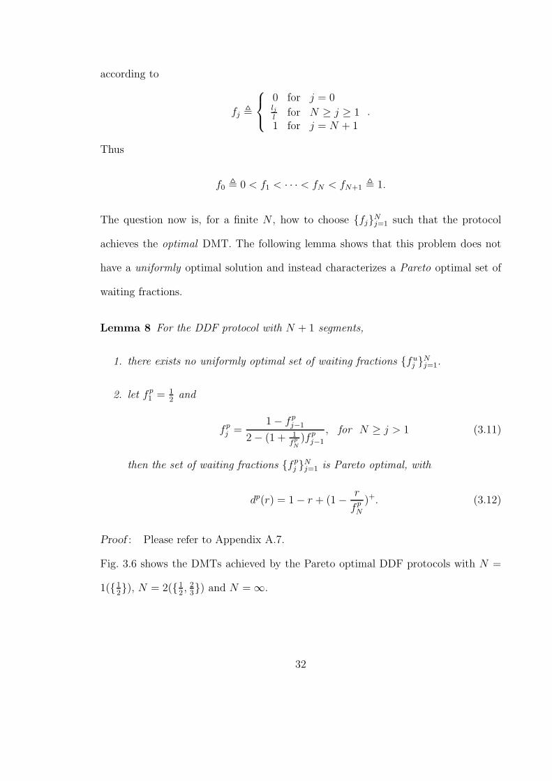
according to
fj ,
0 for j = 0ljl
for N ≥ j ≥ 11 for j = N + 1
.
Thus
f0 , 0 < f1 < · · · < fN < fN+1 , 1.
The question now is, for a finite N , how to choose {fj}Nj=1 such that the protocol
achieves the optimal DMT. The following lemma shows that this problem does not
have a uniformly optimal solution and instead characterizes a Pareto optimal set of
waiting fractions.
Lemma 8 For the DDF protocol with N + 1 segments,
1. there exists no uniformly optimal set of waiting fractions {fuj }
Nj=1.
2. let f p1 = 1
2and
f pj =
1 − f pj−1
2 − (1 + 1fp
N)f p
j−1
, for N ≥ j > 1 (3.11)
then the set of waiting fractions {f pj }
Nj=1 is Pareto optimal, with
dp(r) = 1 − r + (1 −r
f pN
)+. (3.12)
Proof : Please refer to Appendix A.7.
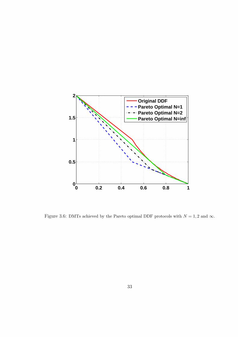
Fig. 3.6 shows the DMTs achieved by the Pareto optimal DDF protocols with N =
1({12}), N = 2({1
2, 2
3}) and N = ∞.
32
0 0.2 0.4 0.6 0.8 10
0.5
1
1.5
2
Original DDFPareto Optimal N=1Pareto Optimal N=2Pareto Optimal N=inf
Figure 3.6: DMTs achieved by the Pareto optimal DDF protocols with N = 1, 2 and ∞.
33
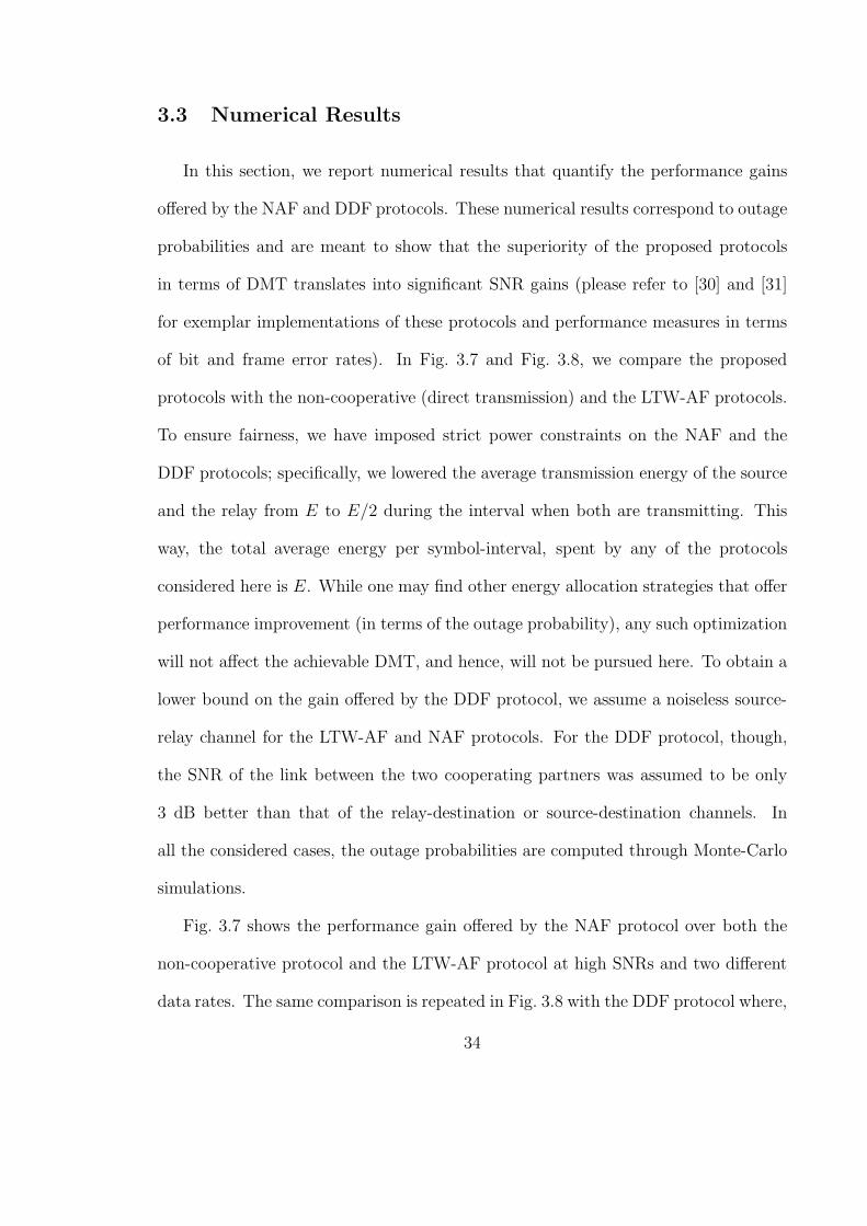
3.3 Numerical Results
In this section, we report numerical results that quantify the performance gains
offered by the NAF and DDF protocols. These numerical results correspond to outage
probabilities and are meant to show that the superiority of the proposed protocols
in terms of DMT translates into significant SNR gains (please refer to [30] and [31]
for exemplar implementations of these protocols and performance measures in terms
of bit and frame error rates). In Fig. 3.7 and Fig. 3.8, we compare the proposed
protocols with the non-cooperative (direct transmission) and the LTW-AF protocols.
To ensure fairness, we have imposed strict power constraints on the NAF and the
DDF protocols; specifically, we lowered the average transmission energy of the source
and the relay from E to E/2 during the interval when both are transmitting. This
way, the total average energy per symbol-interval, spent by any of the protocols
considered here is E. While one may find other energy allocation strategies that offer
performance improvement (in terms of the outage probability), any such optimization
will not affect the achievable DMT, and hence, will not be pursued here. To obtain a
lower bound on the gain offered by the DDF protocol, we assume a noiseless source-
relay channel for the LTW-AF and NAF protocols. For the DDF protocol, though,
the SNR of the link between the two cooperating partners was assumed to be only
3 dB better than that of the relay-destination or source-destination channels. In
all the considered cases, the outage probabilities are computed through Monte-Carlo
simulations.
Fig. 3.7 shows the performance gain offered by the NAF protocol over both the
non-cooperative protocol and the LTW-AF protocol at high SNRs and two different
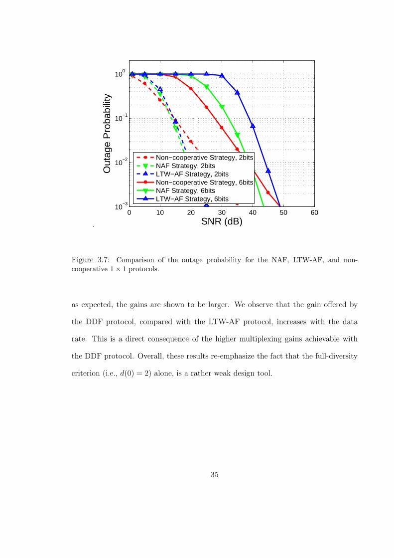
data rates. The same comparison is repeated in Fig. 3.8 with the DDF protocol where,
34
.
0 10 20 30 40 50 6010
−3
10−2
10−1
100
SNR (dB)
Out
age
Pro
babi
lity
Non−cooperative Strategy, 2bitsNAF Strategy, 2bitsLTW−AF Strategy, 2bitsNon−cooperative Strategy, 6bitsNAF Strategy, 6bitsLTW−AF Strategy, 6bits
Figure 3.7: Comparison of the outage probability for the NAF, LTW-AF, and non-cooperative 1 × 1 protocols.
as expected, the gains are shown to be larger. We observe that the gain offered by
the DDF protocol, compared with the LTW-AF protocol, increases with the data
rate. This is a direct consequence of the higher multiplexing gains achievable with
the DDF protocol. Overall, these results re-emphasize the fact that the full-diversity
criterion (i.e., d(0) = 2) alone, is a rather weak design tool.
35
.
0 10 20 30 40 50 6010
−3
10−2
10−1
100
SNR (dB)
Out
age
Pro
babi
lity
Non−cooperative Strategy, 2bitsDDF Strategy, 2bitsLTW−AF Strategy, 2bitsNon−cooperative Strategy, 8bitsDDF Strategy, 8bitsLTW−AF Strategy, 8bits
Figure 3.8: Comparison of the outage probability for the DDF, LTW-AF and non-cooperative 1 × 1 protocols.
36
CHAPTER 4
MULTIUSER COOPERATIVE CHANNELS
In this chapter we consider various multiuser cooperative channels (i.e., CB, MAR
and CMA), and devise appropriate protocols for them.
4.1 Cooperative Broadcast Channel
In the CB scenario, a single source broadcasts to N destinations. This setup is
different from a (non-cooperative) broadcast channel in that in the former scenario,
the destinations are allowed to cooperate through helping one another in receiving
their messages. We assume that the message intended for destination j ∈ {1, · · · , N}
consists of two parts. A common part of rate Rc = rc log ρ BPCU, which is intended
for all of the destinations and an individual part of rate Rj = rj log ρ BPCU, which
is specific to the j-th destination. The total rate is then R = Rc +∑N
j=1Rj and the
multiplexing gain tuple is given by r = (rc, r1, ..., rN). We define the overall diversity
gain d based on the performance of the worst receiver, i.e.
d = minN≥j≥1
{dj},
where we require all the receivers to decode the common information4. Now, as a
first step, one can see that if rc = 0, i.e., if there is no common message, then the
4Clearly this definition does not allow for different Quality of Service (QoS) constraints.
37
techniques developed for the relay channel can be exported to this setting through
a proportional time sharing strategy. With this assumption, all properties of the
NAF and DDF protocols, established in Chapter 3, carry over to this scenario. The
problem becomes slightly more challenging when rc > 0. In fact, it is easy to see
that, for a fixed total rate R, the highest probability of error corresponds to the case
where all destinations are required to decode all the messages. This translates to the
following condition (that applies to any cooperation scheme)
d(rc, r1, r2, ..., rN) ≥ d(rc + r1 + ... + rN , 0, 0, .., 0).
So, we focus the following discussion on this worst case scenario, i.e.,
r = (rc, 0, 0, ..., 0) , for 1 ≥ rc ≥ 0.
As the first observation, we notice that in this scenario, the only AF strategy
that achieves full-rate (i.e., d(r) > 0, ∀r < 1), is the non-cooperative protocol. Any
other AF strategy will require some of the nodes to re-transmit, and therefore not
to listen during parts of the codeword5, which prevents the protocol from achieving
full-rate. Fortunately, this problem can be avoided using a modified version of the
DDF protocol. The reason is that, in the DDF protocol, a node will start helping
only after it has successfully decoded the message. Therefore, cooperation does not
come at the price of reduced rate. The modified DDF protocol, which will be called
the CB-DDF protocol, is very similar to the DDF protocol for the multiple-relay
scenario. The only modification needed, is that now every destination can act as a
relay for the other destinations, based on its instantaneous channel gain. Specifically,
the source transmits during the whole codeword while each destination listens until
5This follows from the half-duplex constraint.
38
the mutual information between its received signal and the signals transmitted by the
source and other destinations exceeds lR. Once a destination decodes the message,
it uses an independent code-book to re-encode the message, which it then transmits
for the rest of the codeword. Similar to the relay channel, it is assumed that every
destination knows the code-books used by the source and other destinations. Also,
the protocol must include a mechanism that keeps every destination informed of
the re-transmission starting times of all the other destinations. Again, in deriving
the following result, we ignore the associated cost of this mechanism, relying on the
asymptotic assumptions.
Theorem 9 The DMT achieved by the CB-DDF protocol with N destinations is given
by
d(rc) =
N(1 − rc),1N
≥ rc ≥ 0,
1 + (N−1)(1−2rc)1−rc
, 12≥ rc ≥
1N,
1−rc
rc, 1 ≥ rc ≥
12.
(4.1)
Proof : Please refer to Appendix A.8.
It is interesting to note that this is exactly the same tradeoff obtained in the
relay channel (compare to (3.8)). This implies that requiring all nodes to decode the
message does not entail a price in terms of the achievable tradeoff.
4.2 Multiple-Access Relay Channel
In the (two-user) MAR channel, a relay is assigned to help the two users transmit
their messages to a common destination. In this scenario, the users are not allowed
to cooperate with one another (e.g, due to practical limitations). In our DDF pro-
tocol for this channel, the two users transmit their individual messages during every
symbol interval in the codeword, while the relay listens to the users until it collects
39
sufficient energy to decode both of them error-free. After decoding, the relay uses an
independent code book to encode the two messages jointly. The encoded symbols are
then transmitted for the rest of the codeword.
We characterize the DMT achieved by the DDF protocol, along with an upper
bound on the achievable DMT in the MAR channel, in Theorem 10. However, before
proceeding further, we need to define the multiplexing gain r and diversity gain d.
Toward this end, we notice that using (2.6), the pair (rj, dj) can be defined for each
of the two users. However, since we consider the symmetric MAR scenario, the two
multiplexing gains r1 and r2 are equal, i.e. r1 = r2. We define the overall multiplexing
r as r , r1 + r2. That is, the multiplexing gain at which the destination receives
information. We further notice that as a result of symmetry, d1 = d2. Therefore, we
define the overall diversity gain d, as d , d1 = d2. We are now ready to state our
main result in this section
Theorem 10 The optimal diversity gain for the symmetric two-user MAR channel
is upper bounded by
dMAR(r) ≤
{2 − r if 1
2≥ r ≥ 0
3(1 − r) if 1 ≥ r ≥ 12
. (4.2)
Furthermore, the DMT achieved by the DDF protocol is lower bounded by
dDDF-MAR(r) ≥
2 − r if 12≥ r ≥ 0
3(1 − r) if 23≥ r ≥ 1
2
21−rr
if 1 ≥ r ≥ 23
. (4.3)
Proof : Please refer to Appendix A.9.
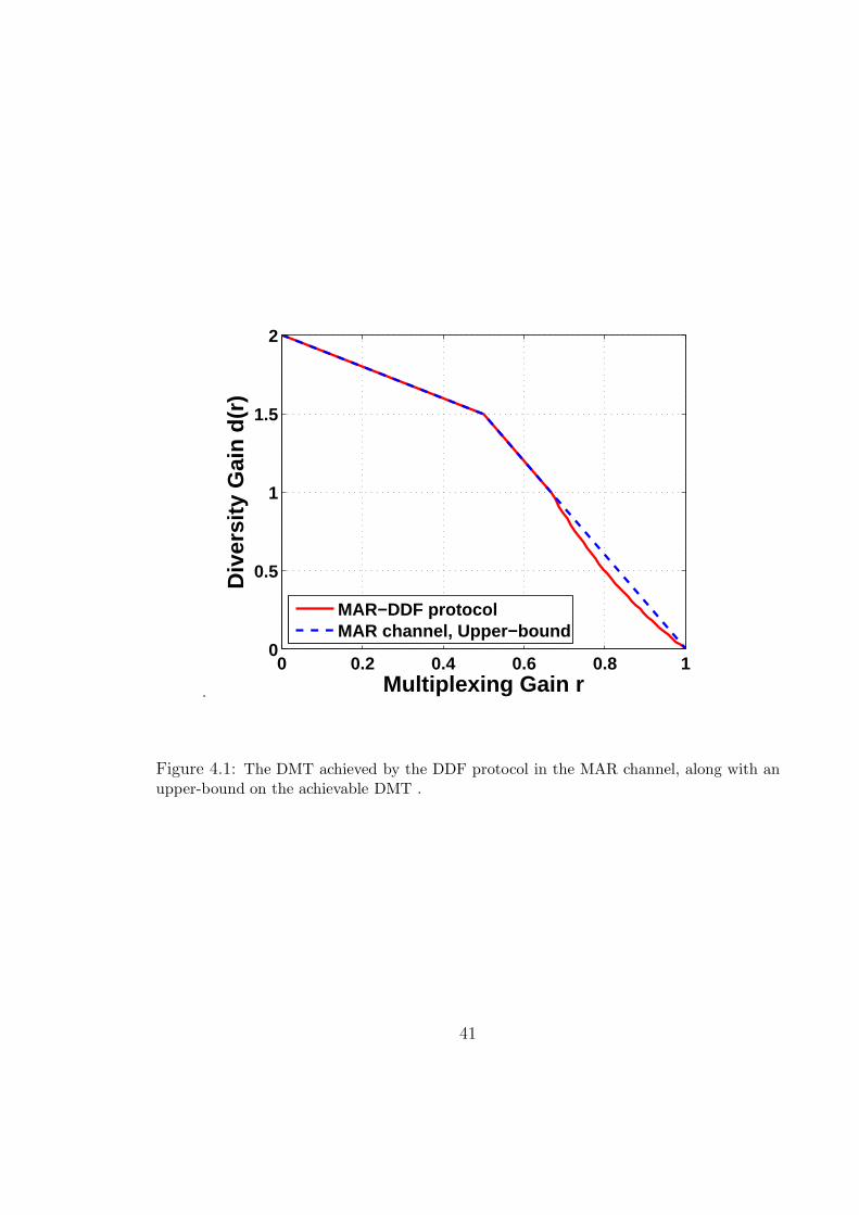
Fig. 4.1 compares the upper and lower bounds in Theorem 10 where the optimality
of the DDF protocol for 2/3 ≥ r ≥ 0 is evident. As a final remark, We note that
the results and ideas in Theorem 10 extend to the N -user MAR channel. However,
40
.
0 0.2 0.4 0.6 0.8 10
0.5
1
1.5
2
Multiplexing Gain r
Div
ersi
ty G
ain
d(r)
MAR−DDF protocolMAR channel, Upper−bound
Figure 4.1: The DMT achieved by the DDF protocol in the MAR channel, along with anupper-bound on the achievable DMT .
41
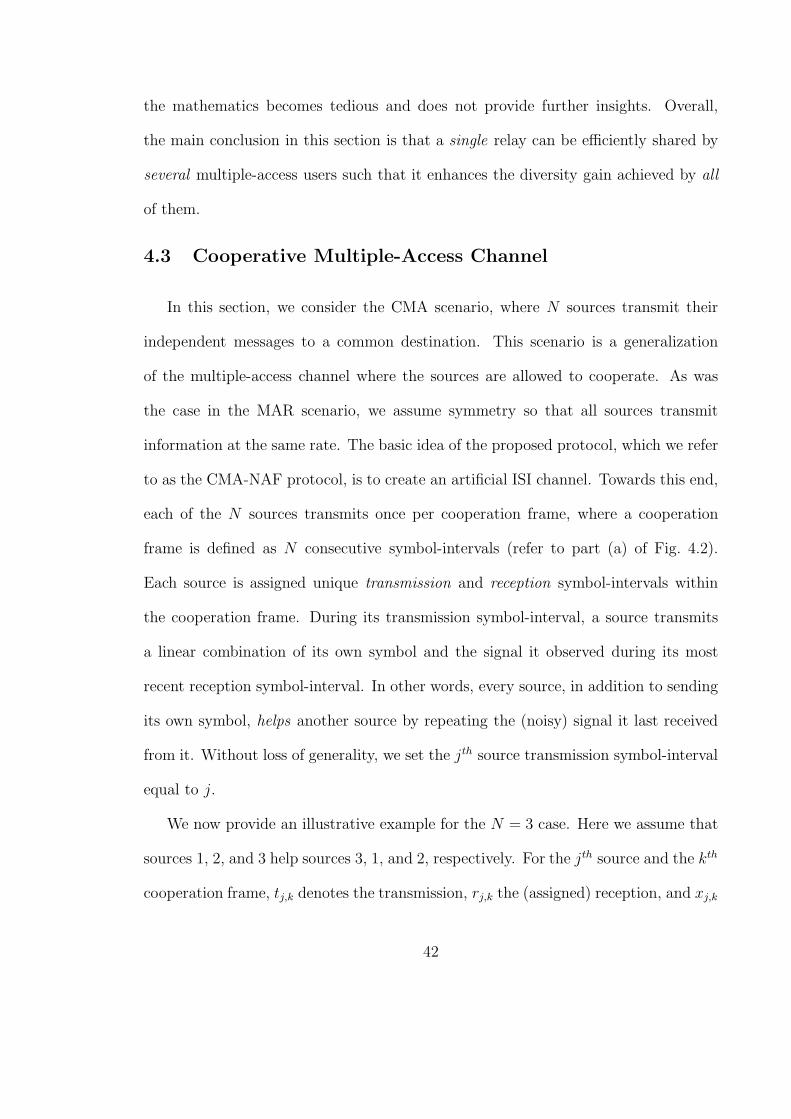
the mathematics becomes tedious and does not provide further insights. Overall,
the main conclusion in this section is that a single relay can be efficiently shared by
several multiple-access users such that it enhances the diversity gain achieved by all
of them.
4.3 Cooperative Multiple-Access Channel
In this section, we consider the CMA scenario, where N sources transmit their
independent messages to a common destination. This scenario is a generalization
of the multiple-access channel where the sources are allowed to cooperate. As was
the case in the MAR scenario, we assume symmetry so that all sources transmit
information at the same rate. The basic idea of the proposed protocol, which we refer
to as the CMA-NAF protocol, is to create an artificial ISI channel. Towards this end,
each of the N sources transmits once per cooperation frame, where a cooperation
frame is defined as N consecutive symbol-intervals (refer to part (a) of Fig. 4.2).
Each source is assigned unique transmission and reception symbol-intervals within
the cooperation frame. During its transmission symbol-interval, a source transmits
a linear combination of its own symbol and the signal it observed during its most
recent reception symbol-interval. In other words, every source, in addition to sending
its own symbol, helps another source by repeating the (noisy) signal it last received
from it. Without loss of generality, we set the jth source transmission symbol-interval
equal to j.
We now provide an illustrative example for the N = 3 case. Here we assume that
sources 1, 2, and 3 help sources 3, 1, and 2, respectively. For the jth source and the kth
cooperation frame, tj,k denotes the transmission, rj,k the (assigned) reception, and xj,k
42
· · ·
· · ·
· · ·
a) Cooperation Frame.
N Symbols
1 2 N
b) Super-Frame.
L Frames
1 2 L
c) Coherence Interval
N − 1 Super-Frames
1 2 N − 1
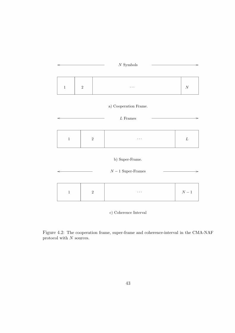
Figure 4.2: The cooperation frame, super-frame and coherence-interval in the CMA-NAFprotocol with N sources.
43
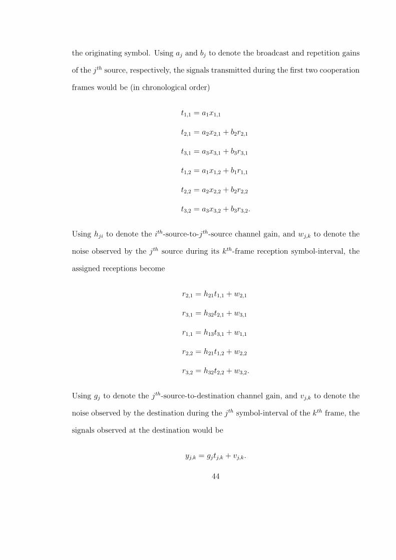
the originating symbol. Using aj and bj to denote the broadcast and repetition gains
of the jth source, respectively, the signals transmitted during the first two cooperation
frames would be (in chronological order)
t1,1 = a1x1,1
t2,1 = a2x2,1 + b2r2,1
t3,1 = a3x3,1 + b3r3,1
t1,2 = a1x1,2 + b1r1,1
t2,2 = a2x2,2 + b2r2,2
t3,2 = a3x3,2 + b3r3,2.
Using hji to denote the ith-source-to-jth-source channel gain, and wj,k to denote the
noise observed by the jth source during its kth-frame reception symbol-interval, the
assigned receptions become
r2,1 = h21t1,1 + w2,1
r3,1 = h32t2,1 + w3,1
r1,1 = h13t3,1 + w1,1
r2,2 = h21t1,2 + w2,2
r3,2 = h32t2,2 + w3,2.
Using gj to denote the jth-source-to-destination channel gain, and vj,k to denote the
noise observed by the destination during the jth symbol-interval of the kth frame, the
signals observed at the destination would be
yj,k = gjtj,k + vj,k.
44
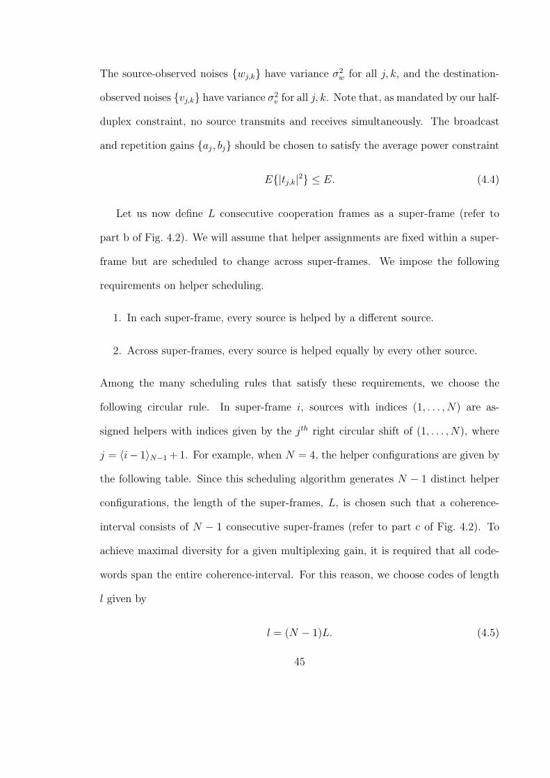
The source-observed noises {wj,k} have variance σ2w for all j, k, and the destination-
observed noises {vj,k} have variance σ2v for all j, k. Note that, as mandated by our half-
duplex constraint, no source transmits and receives simultaneously. The broadcast
and repetition gains {aj , bj} should be chosen to satisfy the average power constraint
E{|tj,k|2} ≤ E. (4.4)
Let us now define L consecutive cooperation frames as a super-frame (refer to
part b of Fig. 4.2). We will assume that helper assignments are fixed within a super-
frame but are scheduled to change across super-frames. We impose the following
requirements on helper scheduling.
1. In each super-frame, every source is helped by a different source.
2. Across super-frames, every source is helped equally by every other source.
Among the many scheduling rules that satisfy these requirements, we choose the
following circular rule. In super-frame i, sources with indices (1, . . . , N) are as-
signed helpers with indices given by the jth right circular shift of (1, . . . , N), where
j = 〈i− 1〉N−1 + 1. For example, when N = 4, the helper configurations are given by
the following table. Since this scheduling algorithm generates N − 1 distinct helper
configurations, the length of the super-frames, L, is chosen such that a coherence-
interval consists of N − 1 consecutive super-frames (refer to part c of Fig. 4.2). To
achieve maximal diversity for a given multiplexing gain, it is required that all code-
words span the entire coherence-interval. For this reason, we choose codes of length
l given by
l = (N − 1)L. (4.5)
45
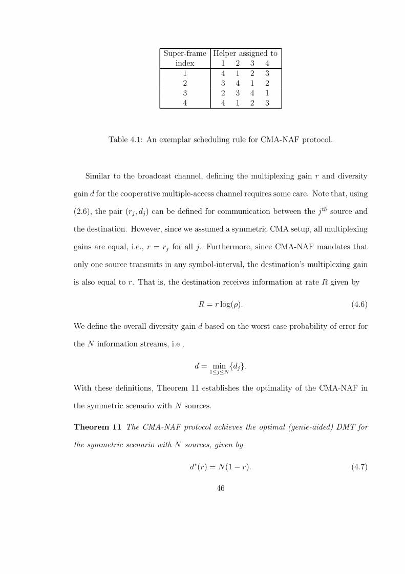
Super-frame Helper assigned toindex 1 2 3 4
1 4 1 2 32 3 4 1 23 2 3 4 14 4 1 2 3
Table 4.1: An exemplar scheduling rule for CMA-NAF protocol.
Similar to the broadcast channel, defining the multiplexing gain r and diversity
gain d for the cooperative multiple-access channel requires some care. Note that, using
(2.6), the pair (rj, dj) can be defined for communication between the jth source and
the destination. However, since we assumed a symmetric CMA setup, all multiplexing
gains are equal, i.e., r = rj for all j. Furthermore, since CMA-NAF mandates that
only one source transmits in any symbol-interval, the destination’s multiplexing gain
is also equal to r. That is, the destination receives information at rate R given by
R = r log(ρ). (4.6)
We define the overall diversity gain d based on the worst case probability of error for
the N information streams, i.e.,
d = min1≤j≤N
{dj}.
With these definitions, Theorem 11 establishes the optimality of the CMA-NAF in
the symmetric scenario with N sources.
Theorem 11 The CMA-NAF protocol achieves the optimal (genie-aided) DMT for
the symmetric scenario with N sources, given by
d∗(r) = N(1 − r). (4.7)
46
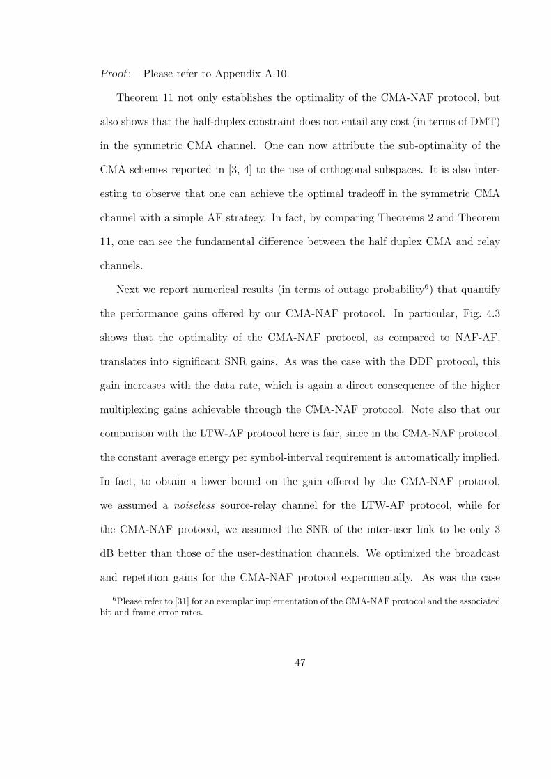
Proof : Please refer to Appendix A.10.
Theorem 11 not only establishes the optimality of the CMA-NAF protocol, but
also shows that the half-duplex constraint does not entail any cost (in terms of DMT)
in the symmetric CMA channel. One can now attribute the sub-optimality of the
CMA schemes reported in [3, 4] to the use of orthogonal subspaces. It is also inter-
esting to observe that one can achieve the optimal tradeoff in the symmetric CMA
channel with a simple AF strategy. In fact, by comparing Theorems 2 and Theorem
11, one can see the fundamental difference between the half duplex CMA and relay
channels.
Next we report numerical results (in terms of outage probability6) that quantify
the performance gains offered by our CMA-NAF protocol. In particular, Fig. 4.3
shows that the optimality of the CMA-NAF protocol, as compared to NAF-AF,
translates into significant SNR gains. As was the case with the DDF protocol, this
gain increases with the data rate, which is again a direct consequence of the higher
multiplexing gains achievable through the CMA-NAF protocol. Note also that our
comparison with the LTW-AF protocol here is fair, since in the CMA-NAF protocol,
the constant average energy per symbol-interval requirement is automatically implied.
In fact, to obtain a lower bound on the gain offered by the CMA-NAF protocol,
we assumed a noiseless source-relay channel for the LTW-AF protocol, while for
the CMA-NAF protocol, we assumed the SNR of the inter-user link to be only 3
dB better than those of the user-destination channels. We optimized the broadcast
and repetition gains for the CMA-NAF protocol experimentally. As was the case
6Please refer to [31] for an exemplar implementation of the CMA-NAF protocol and the associatedbit and frame error rates.
47
.
0 10 20 30 40 50 6010
−3
10−2
10−1
100
SNR (dB)
Out
age
Pro
babi
lity
Genie Aided Strategy, 2bitsCMA−NAF Strategy, 2bitsLTW−AF Strategy, 2bitsGenie Aided Strategy, 8bitsCMA−NAF Strategy, 8bitsLTW−AF Strategy, 8bits
Figure 4.3: Comparison of the outage probability for the CMA-NAF, LTW-AF and genie-aided 2 × 1 protocols (N = 2).
with relay protocols, the outage probabilities were computed through Monte-Carlo
simulations.
Also depicted in Fig. 4.3 are the outage probability curves for the genie-aided
strategy (i.e., 2 × 1 MIMO). It is interesting to notice that the gap between the
outage curves of the CMA-NAF and genie-aided strategies is less than 3 dB when the
date rate is equal to 2 BPCU.
48
CHAPTER 5
ARQ COOPERATIVE CHANNELS
In this chapter we consider ARQ cooperative channels where users, after each
transmission round, are provided with ACK/NACK signals indicating success or fail-
ure of destination in decoding their messages. As we will show, utilization of ARQ
techniques not only improves the DMT achieved by some of the proposed protocols
(e.g., DDF relay and MAR), but also provides opportunities for cooperation that are
otherwise unavailable (e.g., DDF CVMA protocol). We start, though, with a few
definitions and assumptions that are used throughout the chapter.
• We denote the maximum allowable number of ARQ rounds by L, where L =
1 corresponds to the non-ARQ scenario. A transmission round consists of l
consecutive symbol-intervals. In order to highlight the benefits of ARQ, as
opposed to temporal interleaving, we adopt the long-term static channel model
of [29] where all the ARQ rounds corresponding to a certain message take place
over the same coherence-interval.
• We denote the first-round rate of transmission (at destination) by R1 and the
average throughput by η. These two quantities are related through [29]
η =R1
1 +∑L−1
ℓ=1 p(ℓ), (5.1)
49
where p(ℓ) is the probability that the destination requests for the (ℓ+1)th round
of transmission. We define the first-round multiplexing gain, r1, and effective
multiplexing gain, re, as
r1 , limρ→∞
R1
log ρ, re , lim
ρ→∞
η
log ρ. (5.2)
From (5.1), we note that if {p(ℓ)}L−1ℓ=1 decay polynomially with ρ, then η=R1
and thus re = r1.
• As was the case in non-ARQ scenarios, we adopt the coherent transmission
paradigm where only the receiving node of any link knows the channel gain;
Except for the ACK/NACK feedback bits, no other CSI is available to the
transmitting nodes.
• In characterizing DMT for ARQ cooperative protocols, we replace r with the ef-
fective multiplexing gain re to capture the variable-rate nature of ARQ schemes
[29].
5.1 ARQ Multiple-Access Relay Channel
In this section, we adopt the DDF protocol to the ARQ MAR channel and prove
its optimality. The proposed ARQ-DDF protocol is identical to the one devised for the
MAR channel (refer to Section.4.2), except that users only move on to sending their
next message if either all of them have received ACK signals, or that the maximum
allowable number of ARQ rounds, L, has already been requested. To prove the
optimality of this protocol, we first prove the optimality of the ARQ-DDF protocol
in the relay channel (i.e., an ARQ MAR channel with a single user). The proof for
this result provides the machinery necessary to handle the ARQ mechanism. Then,
50
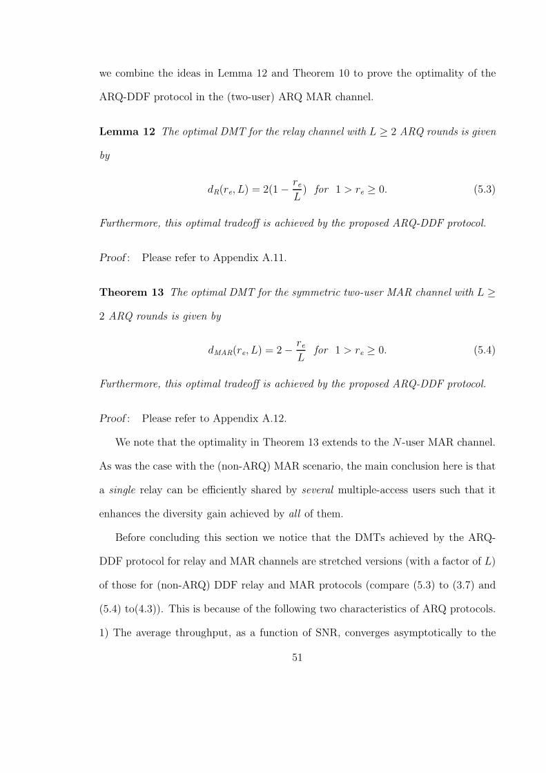
we combine the ideas in Lemma 12 and Theorem 10 to prove the optimality of the
ARQ-DDF protocol in the (two-user) ARQ MAR channel.
Lemma 12 The optimal DMT for the relay channel with L ≥ 2 ARQ rounds is given
by
dR(re, L) = 2(1 −reL
) for 1 > re ≥ 0. (5.3)
Furthermore, this optimal tradeoff is achieved by the proposed ARQ-DDF protocol.
Proof : Please refer to Appendix A.11.
Theorem 13 The optimal DMT for the symmetric two-user MAR channel with L ≥
2 ARQ rounds is given by
dMAR(re, L) = 2 −reL
for 1 > re ≥ 0. (5.4)
Furthermore, this optimal tradeoff is achieved by the proposed ARQ-DDF protocol.
Proof : Please refer to Appendix A.12.
We note that the optimality in Theorem 13 extends to the N -user MAR channel.
As was the case with the (non-ARQ) MAR scenario, the main conclusion here is that
a single relay can be efficiently shared by several multiple-access users such that it
enhances the diversity gain achieved by all of them.
Before concluding this section we notice that the DMTs achieved by the ARQ-
DDF protocol for relay and MAR channels are stretched versions (with a factor of L)
of those for (non-ARQ) DDF relay and MAR protocols (compare (5.3) to (3.7) and
(5.4) to(4.3)). This is because of the following two characteristics of ARQ protocols.
1) The average throughput, as a function of SNR, converges asymptotically to the
51
throughput corresponding to one round of transmission, and 2) the error event is
dominated by those for which L rounds of transmission has been requested. As a
result, the ARQ protocols enjoy the diversity gain that the non-ARQ versions achieve
at a multiplexing gain L times smaller.
5.2 ARQ Cooperative Vector Multiple-Access Channel
In the cooperative vector multiple access (CVMA) channel, the two single-antenna
users are allowed to assist each other, as long as they do not violate the half duplex
constraint. The challenge in this scenario stems from the availability of two receiving
antennas at the destination, which increases the channel’s degrees of freedom to two.
Loosely speaking, in order to exploit these two degrees of freedom, the two users
need to transmit new independent symbols continuously, which prevents them from
cooperation under the half duplex constraint (non-ARQ case). More rigorously, it is
straightforward to see that with L = 1, any half-duplex cooperation protocol that
achieves full diversity (i.e., d(0) = 3), falls short of achieving full rate (i.e., d(r) > 0,
for all r < 2). To get around this problem, in the case of L ≥ 2, we purposefully
instruct the users not to cooperate in the first round of transmission. In fact, a user
continues transmitting its message while it receives NACK signals. Only when a
user receives an ACK signal, it starts listening to the other user (assuming the other
user has not been successfully decoded yet). Once the cooperating user decodes the
message of its partner, it starts helping (i.e., the typical DDF methodology). The
following result establishes lower and upper bounds on the DMT achieved by this
protocol.
52
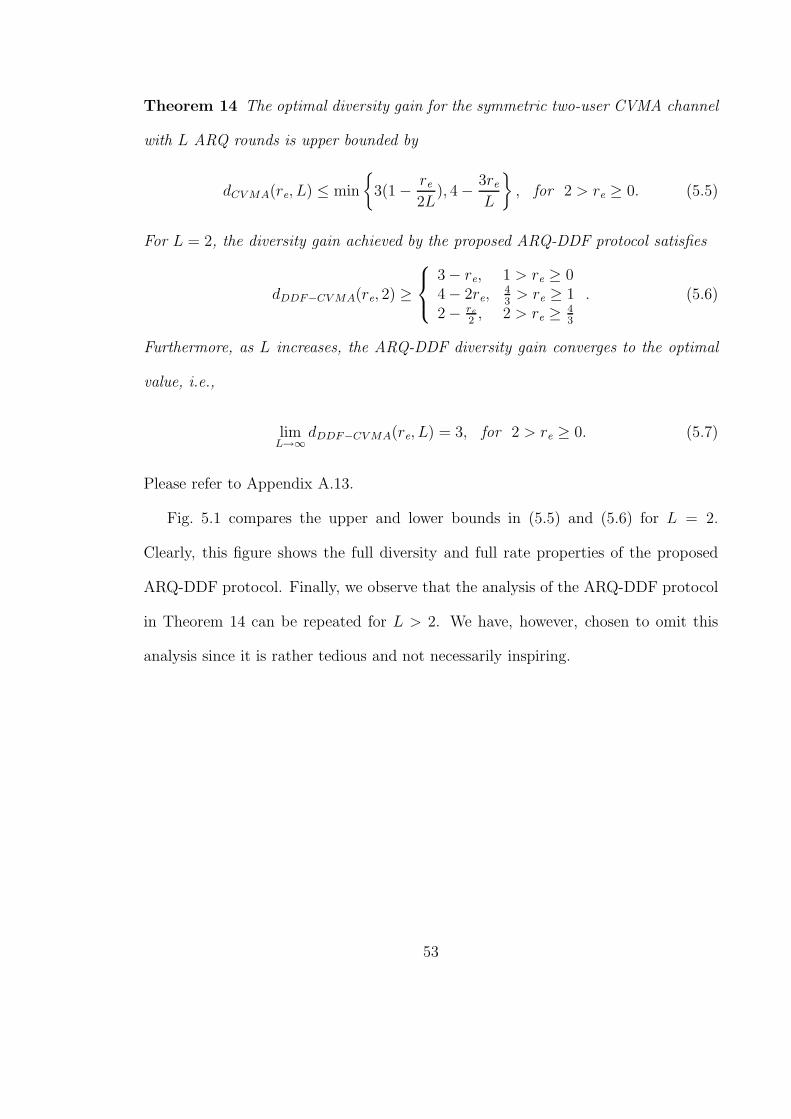
Theorem 14 The optimal diversity gain for the symmetric two-user CVMA channel
with L ARQ rounds is upper bounded by
dCV MA(re, L) ≤ min
{
3(1 −re2L
), 4 −3reL
}
, for 2 > re ≥ 0. (5.5)
For L = 2, the diversity gain achieved by the proposed ARQ-DDF protocol satisfies
dDDF−CV MA(re, 2) ≥
3 − re, 1 > re ≥ 04 − 2re,
43> re ≥ 1
2 − re2, 2 > re ≥
43
. (5.6)
Furthermore, as L increases, the ARQ-DDF diversity gain converges to the optimal
value, i.e.,
limL→∞
dDDF−CV MA(re, L) = 3, for 2 > re ≥ 0. (5.7)
Please refer to Appendix A.13.
Fig. 5.1 compares the upper and lower bounds in (5.5) and (5.6) for L = 2.
Clearly, this figure shows the full diversity and full rate properties of the proposed
ARQ-DDF protocol. Finally, we observe that the analysis of the ARQ-DDF protocol
in Theorem 14 can be repeated for L > 2. We have, however, chosen to omit this
analysis since it is rather tedious and not necessarily inspiring.
53
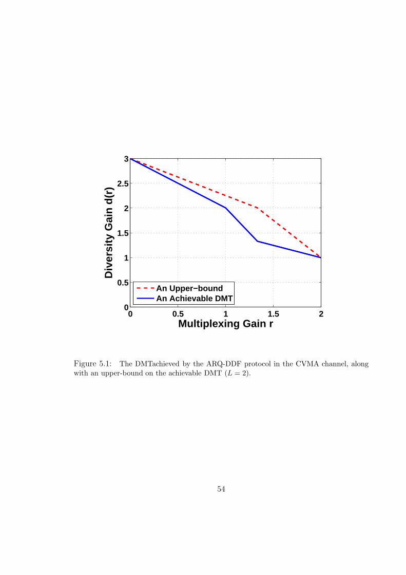
0 0.5 1 1.5 20
0.5
1
1.5
2
2.5
3
Multiplexing Gain r
Div
ersi
ty G
ain
d(r)
An Upper−boundAn Achievable DMT
Figure 5.1: The DMTachieved by the ARQ-DDF protocol in the CVMA channel, alongwith an upper-bound on the achievable DMT (L = 2).
54
CHAPTER 6
THE THROUGHPUT-RELIABILITY TRADEOFF
6.1 Problem Formulation
This chapter revolves around the following question: What does a 3 dB increase in
SNR buy in an outage limited MIMO channel? In an AWGN setting, it is well known
that a 3 dB increase in SNR translates into an extra bit in channel capacity in the high
SNR regime. The scenario considered in this chapter, however, is more involved. We
study an outage limited channel where the randomness of the instantaneous mutual
information results in a non-zero lower bound on the probability of error, for non-zero
constant transmission rates. Hence, a fundamental tradeoff between the throughput,
as quantified by the transmission rate, and reliability, as quantified by the so-called
outage probability, arises. Our work explores this tradeoff in the high SNR regime.
To be more specific, we consider a MIMO wireless communication system with
m transmit and n receive antennas. We adopt a quasi-static flat-fading setup where
the path gains remain constant over l consecutive symbol-intervals (i.e., a block),
but change independently from one block to another. We further assume a coherent
communication model implying the availability of channel state information (CSI)
only at the receiver. Under these assumptions, the channel input-output relation is
55
given by:
y =
√ρ
mHx + w. (6.1)
In (6.1), y ∈ Cn has entries yi representing the signal received at antenna i ∈
{1, · · · , n}, x ∈ Cm has entries xj denoting the signal transmitted by antenna j ∈
{1, · · · , m}, H ∈ Cn×m has entries hij which represents the path gain between receive
antenna i ∈ {1, · · · , n} and transmit antenna j ∈ {1, · · · , m}, and w ∈ Cn represents
the unit-variance additive white Gaussian noise. We model {hij} as i.i.d zero-mean
and unit-variance complex Gaussian random variables. Finally, ρ corresponds to the
SNR at each receive antenna.
Our work builds on Zheng and Tse’s formulation of the DMT [17]. This formula-
tion assumes a family of space-time codes {C(ρ)} indexed by their operating SNR ρ,
such that the code C(ρ) has rate R(ρ) BPCU, and error probability Pe(ρ). For this
family, the multiplexing gain r and the diversity gain d are defined by
r , limρ→∞
R(ρ)
log ρand d , − lim
ρ→∞
logPe(ρ)
log ρ. (6.2)
The optimal DMT yields the maximum possible diversity gain for every value of r.
The main result of [17] is summarized in the following theorem:
Theorem 15 The optimal diversity gain for the coherent quasi-static MIMO channel
with m transmit and n receive antennas, at multiplexing gain r, is given by d(r) =
f(r), where f(·) is the piecewise linear function joining the points (k, (m−k)(n−k))
for k = 0, . . . ,min{m,n}. Moreover, there exists a code that achieves d(r) for all
block lengths l ≥ m+ n− 1.
In the sequel, we will use the notation dmax = mn and rmax = min{m,n}. To motivate
our work, we use the DMT to make a first attempt towards answering our central
56
question on the utility of a 3 dB SNR gain in quasi-static MIMO channels. Using
the extreme points of the tradeoff curve, i.e., (0, dmax) and (rmax, 0), a reasonable
conjecture is
1. At high enough SNRs, one can fix the transmission rate and obtain a decay, by
a factor of 10−dmax , in the outage probability, for every 10 dB gain in SNR.
2. At high enough SNRs, one can fix the outage probability and obtain a rate
increase of rmax BPCU for every 3 dB gain in SNR.
Fig. 6.1 and Fig. 6.2 examine the validity of this conjecture in a 2 × 2 MIMO chan-
nel. In these figures, the transmission rates and SNR ranges are carefully chosen to
illustrate the following points.
1. The slope of the outage probability curves in Fig. 6.1 is shown to approach the
asymptotic value of dmax = 4, on the log-log scale, as predicted by the first part
of our conjecture. The surprising observation, however, is that for a constant
outage probability a 4.5 dB gain in SNR is needed to obtain an rmax = 2 BPCU
increase in the throughput (To avoid fractions of a dB, the figure shows a 9
dB spacing for a 4 BPCU throughput increase). This contrasts the second part
of our conjecture which predicts the need for only 3 dB for every 2 BPCU.
More interestingly, this 4.5 dB horizontal spacing seems to persist as the SNR
increases.
2. Fig. 6.2, on the other hand, comes in close agreement with the second part of our
conjecture. Here, the horizontal spacing, for a 2 BPCU increase in throughput,
is seen to be 3 dB. The disagreement in this case, however, is exhibited in the
57
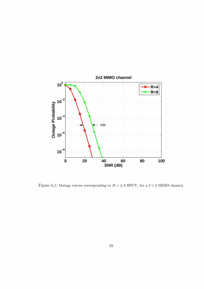
0 20 40 60 80 100
10−8
10−6
10−4
10−2
100
SNR (dB)
Out
age
Pro
babi
lity
2x2 MIMO channel
R=4R=8
9dB
Figure 6.1: Outage curves corresponding to R = 4, 8 BPCU, for a 2 × 2 MIMO channel.
58
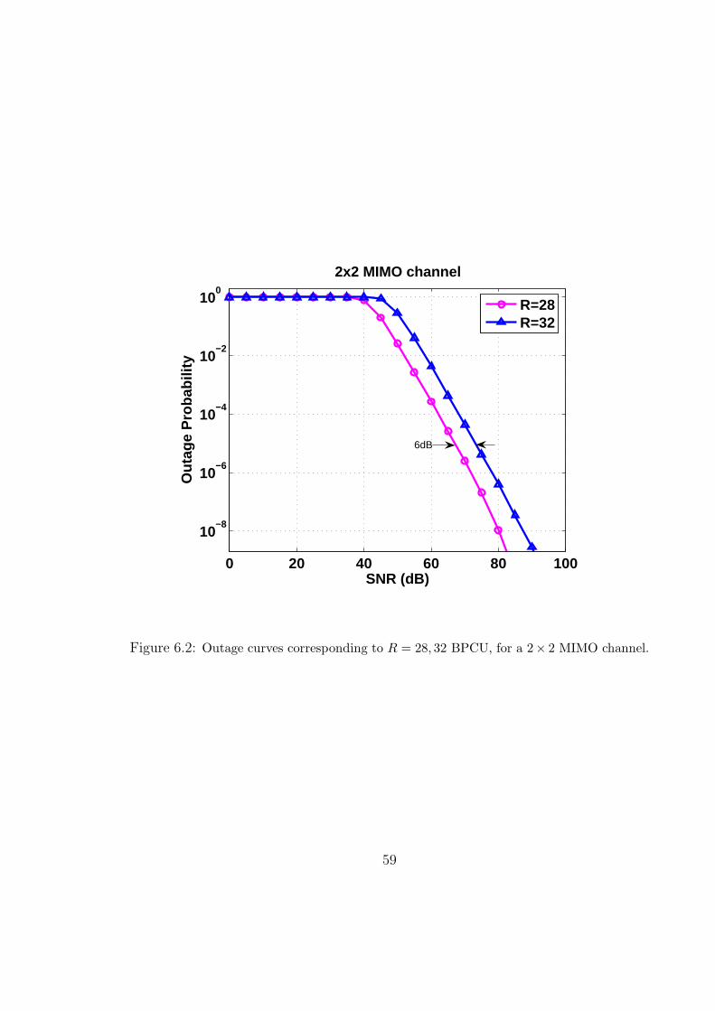
0 20 40 60 80 100
10−8
10−6
10−4
10−2
100
SNR (dB)
Out
age
Pro
babi
lity
2x2 MIMO channel
R=28R=32
6dB
Figure 6.2: Outage curves corresponding to R = 28, 32 BPCU, for a 2× 2 MIMO channel.
59
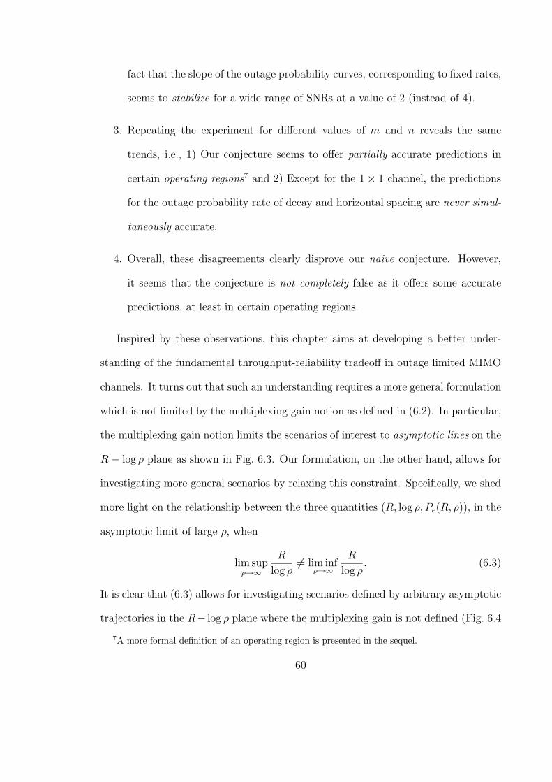
fact that the slope of the outage probability curves, corresponding to fixed rates,
seems to stabilize for a wide range of SNRs at a value of 2 (instead of 4).
3. Repeating the experiment for different values of m and n reveals the same
trends, i.e., 1) Our conjecture seems to offer partially accurate predictions in
certain operating regions7 and 2) Except for the 1 × 1 channel, the predictions
for the outage probability rate of decay and horizontal spacing are never simul-
taneously accurate.
4. Overall, these disagreements clearly disprove our naive conjecture. However,
it seems that the conjecture is not completely false as it offers some accurate
predictions, at least in certain operating regions.
Inspired by these observations, this chapter aims at developing a better under-
standing of the fundamental throughput-reliability tradeoff in outage limited MIMO
channels. It turns out that such an understanding requires a more general formulation
which is not limited by the multiplexing gain notion as defined in (6.2). In particular,
the multiplexing gain notion limits the scenarios of interest to asymptotic lines on the
R− log ρ plane as shown in Fig. 6.3. Our formulation, on the other hand, allows for
investigating more general scenarios by relaxing this constraint. Specifically, we shed
more light on the relationship between the three quantities (R, log ρ, Pe(R, ρ)), in the
asymptotic limit of large ρ, when
lim supρ→∞
R
log ρ6= lim inf
ρ→∞
R
log ρ. (6.3)
It is clear that (6.3) allows for investigating scenarios defined by arbitrary asymptotic
trajectories in the R− log ρ plane where the multiplexing gain is not defined (Fig. 6.4
7A more formal definition of an operating region is presented in the sequel.
60
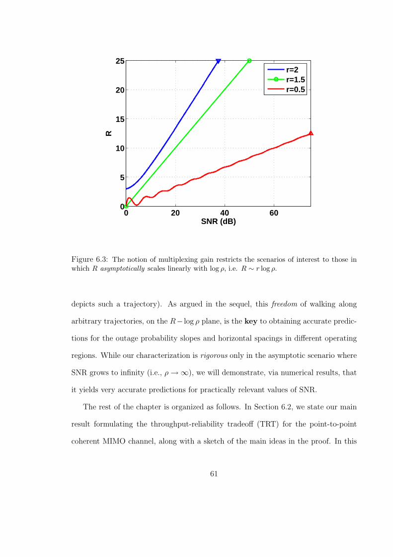
0 20 40 600
5
10
15
20
25
SNR (dB)
R
r=2r=1.5r=0.5
Figure 6.3: The notion of multiplexing gain restricts the scenarios of interest to those inwhich R asymptotically scales linearly with log ρ, i.e. R ∼ r log ρ.
depicts such a trajectory). As argued in the sequel, this freedom of walking along
arbitrary trajectories, on the R− log ρ plane, is the key to obtaining accurate predic-
tions for the outage probability slopes and horizontal spacings in different operating
regions. While our characterization is rigorous only in the asymptotic scenario where
SNR grows to infinity (i.e., ρ→ ∞), we will demonstrate, via numerical results, that
it yields very accurate predictions for practically relevant values of SNR.
The rest of the chapter is organized as follows. In Section 6.2, we state our main
result formulating the throughput-reliability tradeoff (TRT) for the point-to-point
coherent MIMO channel, along with a sketch of the main ideas in the proof. In this
61
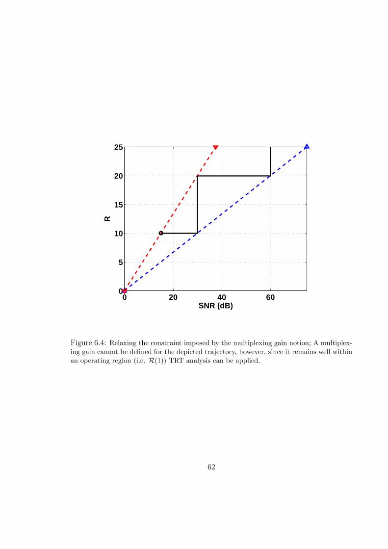
0 20 40 600
5
10
15
20
25
SNR (dB)
R
Figure 6.4: Relaxing the constraint imposed by the multiplexing gain notion; A multiplex-ing gain cannot be defined for the depicted trajectory, however, since it remains well withinan operating region (i.e. R(1)) TRT analysis can be applied.
62
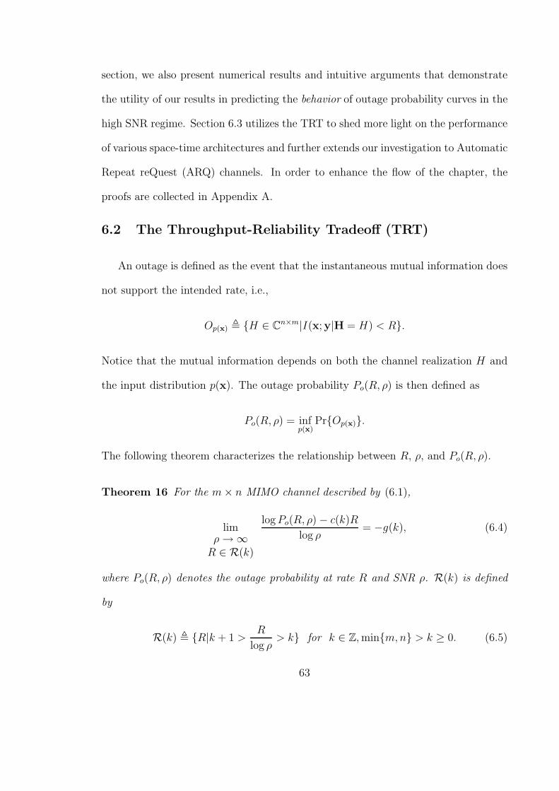
section, we also present numerical results and intuitive arguments that demonstrate
the utility of our results in predicting the behavior of outage probability curves in the
high SNR regime. Section 6.3 utilizes the TRT to shed more light on the performance
of various space-time architectures and further extends our investigation to Automatic
Repeat reQuest (ARQ) channels. In order to enhance the flow of the chapter, the
proofs are collected in Appendix A.
6.2 The Throughput-Reliability Tradeoff (TRT)
An outage is defined as the event that the instantaneous mutual information does
not support the intended rate, i.e.,
Op(x) , {H ∈ Cn×m|I(x;y|H = H) < R}.
Notice that the mutual information depends on both the channel realization H and
the input distribution p(x). The outage probability Po(R, ρ) is then defined as
Po(R, ρ) = infp(x)
Pr{Op(x)}.
The following theorem characterizes the relationship between R, ρ, and Po(R, ρ).
Theorem 16 For the m× n MIMO channel described by (6.1),
limρ→ ∞R ∈ R(k)
logPo(R, ρ) − c(k)R
log ρ= −g(k), (6.4)
where Po(R, ρ) denotes the outage probability at rate R and SNR ρ. R(k) is defined
by
R(k) , {R|k + 1 >R
log ρ> k} for k ∈ Z,min{m,n} > k ≥ 0. (6.5)
63

In (6.4), c(k) and g(k) are given by
c(k) , m+ n− (2k + 1), (6.6)
and
g(k) , mn− k(k + 1). (6.7)
Moreover, in the degenerate case R > min{m,n} log ρ, limρ→∞ logPo(R, ρ)/ log ρ = 0.
We refer to g(k) as the reliability gain coefficient and t(k) , g(k)/c(k) as the through-
put gain coefficient.
Proof : (Sketch) Our proof follows the same lines as the proof of Theorem 15 in
[17] except for the fundamental challenge that the multiplexing gain is not defined
here. To handle this challenge, we judicially choose the region R(k) and find a lower
bound on
lim infρ→ ∞R ∈ R(k)
logPo(R, ρ) − c(k)R
log ρ,
and an upper bound on
lim supρ→ ∞R ∈ R(k)
logPo(R, ρ) − c(k)R
log ρ
and show that the two bounds coincide for the choice of c(k) and g(k) given by (6.6)
and (6.7), respectively. The detailed proof is reported in the Appendix A.14.
It is immediate to check that if the multiplexing gain is well defined, i.e., if
r = limρ→∞
R(ρ)
log ρ
64
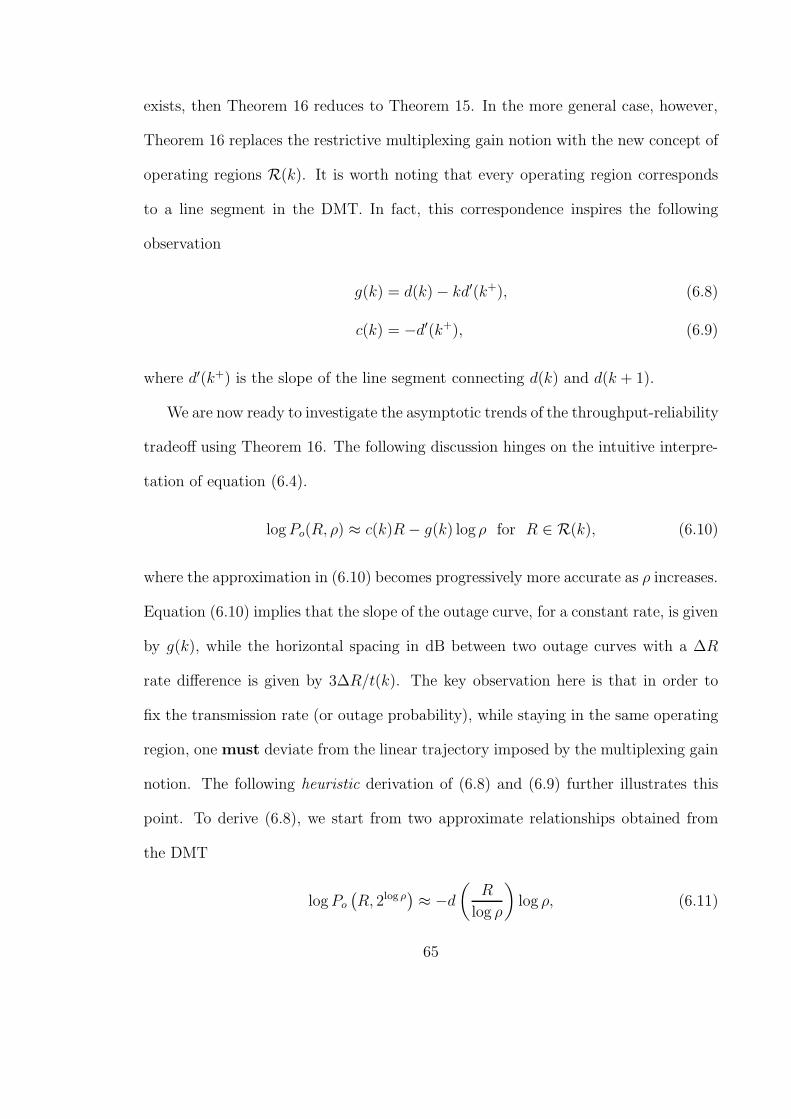
exists, then Theorem 16 reduces to Theorem 15. In the more general case, however,
Theorem 16 replaces the restrictive multiplexing gain notion with the new concept of
operating regions R(k). It is worth noting that every operating region corresponds
to a line segment in the DMT. In fact, this correspondence inspires the following
observation
g(k) = d(k) − kd′(k+), (6.8)
c(k) = −d′(k+), (6.9)
where d′(k+) is the slope of the line segment connecting d(k) and d(k + 1).
We are now ready to investigate the asymptotic trends of the throughput-reliability
tradeoff using Theorem 16. The following discussion hinges on the intuitive interpre-
tation of equation (6.4).
logPo(R, ρ) ≈ c(k)R− g(k) log ρ for R ∈ R(k), (6.10)
where the approximation in (6.10) becomes progressively more accurate as ρ increases.
Equation (6.10) implies that the slope of the outage curve, for a constant rate, is given
by g(k), while the horizontal spacing in dB between two outage curves with a ∆R
rate difference is given by 3∆R/t(k). The key observation here is that in order to
fix the transmission rate (or outage probability), while staying in the same operating
region, one must deviate from the linear trajectory imposed by the multiplexing gain
notion. The following heuristic derivation of (6.8) and (6.9) further illustrates this
point. To derive (6.8), we start from two approximate relationships obtained from
the DMT
logPo
(R, 2log ρ
)≈ −d
(R
log ρ
)
log ρ, (6.11)
65

logPo
(R, 2log ρ+∆log ρ
)≈ −d
(R
log ρ+ ∆ log ρ
)
(log ρ+ ∆ log ρ). (6.12)
We further approximate d(
Rlog ρ+∆ log ρ
)
with the first two terms of its Taylor series
expansion, i.e.,
d
(R
log ρ+ ∆ log ρ
)
≈ d
(R
log ρ
)
−R× ∆ log ρ
log ρ(log ρ+ ∆ log ρ)d′(
R
log ρ
)
, (6.13)
Now (6.13), together with (6.11) and (6.12), gives
logPo(R, 2log ρ) − logPo(R, 2
log ρ+∆ log ρ)
∆ log ρ≈ d
(R
log ρ
)
−R
log ρd′(
R
log ρ
)
. (6.14)
Realizing that the left-hand side of (6.14) gives the slope of Po(R, ρ) with respect to
ρ, i.e. g(k), and that d(r) − rd′(r) remains constant over the line segments of d(r),
we get (6.8). Deriving (6.9) follows the same lines. In particular, we first compute
the horizontal spacing, ∆ log ρ, between the outage curves corresponding to rates R
and R + ∆R. For this purpose, we use (6.11) to write
logPo
(R + ∆R, 2log ρ+∆ log ρ
)≈ −d
(R + ∆R
log ρ+ ∆ log ρ
)
(log ρ+ ∆ log ρ) (6.15)
Then we expand d( R+∆Rlog ρ+∆log ρ
) in a way similar to (6.13) and equate (6.11) with (6.15)
to get
∆ log ρ ≈−d′( R
log ρ)
d( Rlog ρ
) − Rlog ρ
d′( Rlog ρ
)∆R,
∆ log ρ ≈−d′( R
log ρ)
g(k)∆R. (6.16)
Realizing that ∆ log ρ = c(k)g(k)
∆R, and that d′(r) remains constant over the line seg-
ments of d(r), we get (6.9).
Revisiting our naive conjecture, we can now see that g(0) = mn = dmax which
agrees with the first part, while t(min{n,m}−1) = min{m,n} = rmax agrees with the
66
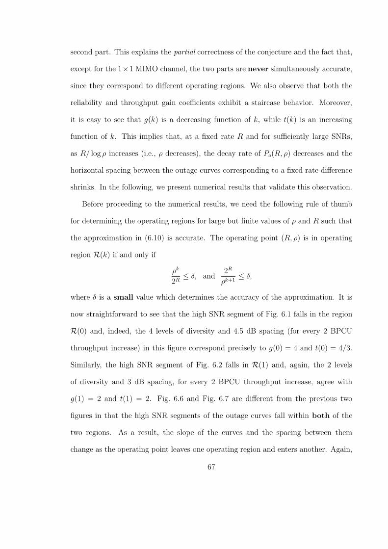
second part. This explains the partial correctness of the conjecture and the fact that,
except for the 1×1 MIMO channel, the two parts are never simultaneously accurate,
since they correspond to different operating regions. We also observe that both the
reliability and throughput gain coefficients exhibit a staircase behavior. Moreover,
it is easy to see that g(k) is a decreasing function of k, while t(k) is an increasing
function of k. This implies that, at a fixed rate R and for sufficiently large SNRs,
as R/ log ρ increases (i.e., ρ decreases), the decay rate of Po(R, ρ) decreases and the
horizontal spacing between the outage curves corresponding to a fixed rate difference
shrinks. In the following, we present numerical results that validate this observation.
Before proceeding to the numerical results, we need the following rule of thumb
for determining the operating regions for large but finite values of ρ and R such that
the approximation in (6.10) is accurate. The operating point (R, ρ) is in operating
region R(k) if and only if
ρk
2R≤ δ, and
2R
ρk+1≤ δ,
where δ is a small value which determines the accuracy of the approximation. It is
now straightforward to see that the high SNR segment of Fig. 6.1 falls in the region
R(0) and, indeed, the 4 levels of diversity and 4.5 dB spacing (for every 2 BPCU
throughput increase) in this figure correspond precisely to g(0) = 4 and t(0) = 4/3.
Similarly, the high SNR segment of Fig. 6.2 falls in R(1) and, again, the 2 levels
of diversity and 3 dB spacing, for every 2 BPCU throughput increase, agree with
g(1) = 2 and t(1) = 2. Fig. 6.6 and Fig. 6.7 are different from the previous two
figures in that the high SNR segments of the outage curves fall within both of the
two regions. As a result, the slope of the curves and the spacing between them
change as the operating point leaves one operating region and enters another. Again,
67
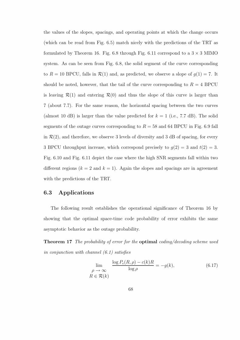
the values of the slopes, spacings, and operating points at which the change occurs
(which can be read from Fig. 6.5) match nicely with the predictions of the TRT as
formulated by Theorem 16. Fig. 6.8 through Fig. 6.11 correspond to a 3 × 3 MIMO
system. As can be seen from Fig. 6.8, the solid segment of the curve corresponding
to R = 10 BPCU, falls in R(1) and, as predicted, we observe a slope of g(1) = 7. It
should be noted, however, that the tail of the curve corresponding to R = 4 BPCU
is leaving R(1) and entering R(0) and thus the slope of this curve is larger than
7 (about 7.7). For the same reason, the horizontal spacing between the two curves
(almost 10 dB) is larger than the value predicted for k = 1 (i.e., 7.7 dB). The solid
segments of the outage curves corresponding to R = 58 and 64 BPCU in Fig. 6.9 fall
in R(2), and therefore, we observe 3 levels of diversity and 3 dB of spacing, for every
3 BPCU throughput increase, which correspond precisely to g(2) = 3 and t(2) = 3.
Fig. 6.10 and Fig. 6.11 depict the case where the high SNR segments fall within two
different regions (k = 2 and k = 1). Again the slopes and spacings are in agreement
with the predictions of the TRT.
6.3 Applications
The following result establishes the operational significance of Theorem 16 by
showing that the optimal space-time code probability of error exhibits the same
asymptotic behavior as the outage probability.
Theorem 17 The probability of error for the optimal coding/decoding scheme used
in conjunction with channel (6.1) satisfies
limρ→ ∞R ∈ R(k)
logPe(R, ρ) − c(k)R
log ρ= −g(k), (6.17)
68
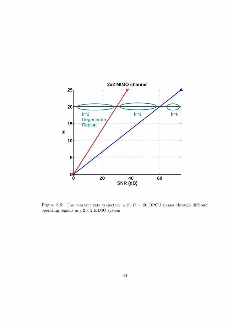
0 20 40 600
5
10
15
20
25
SNR (dB)
R
2x2 MIMO channel
k=2DegenerateRegion
k=1 k=0
Figure 6.5: The constant rate trajectory with R = 20 BPCU passes through differentoperating regions in a 2 × 2 MIMO system
69
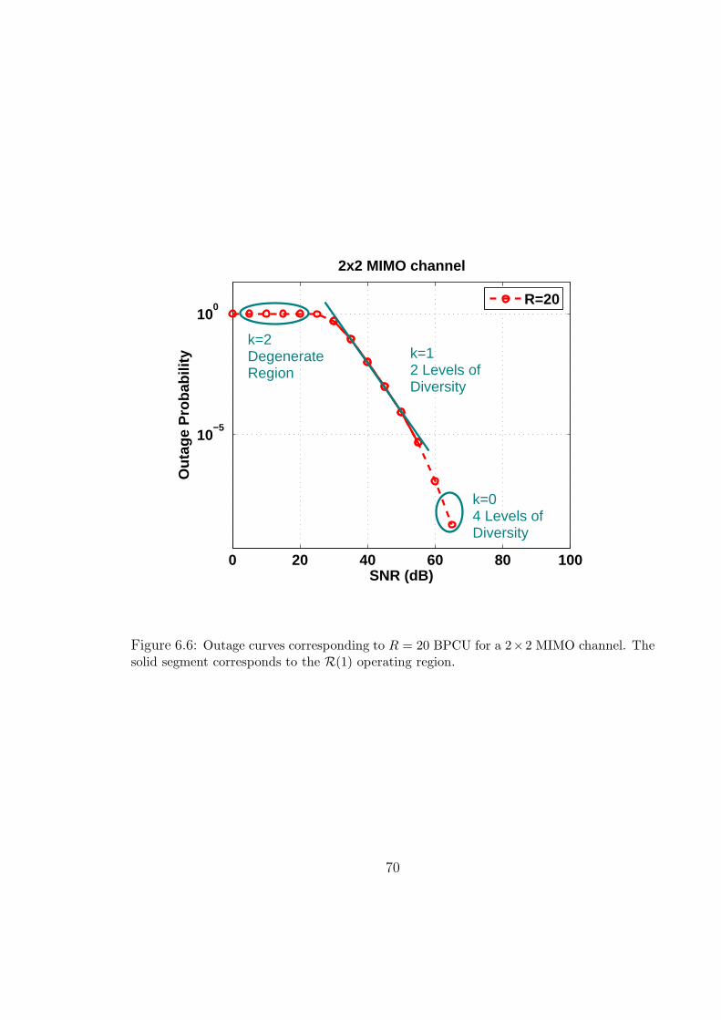
0 20 40 60 80 100
10−5
100
SNR (dB)
Out
age
Pro
babi
lity
2x2 MIMO channel
R=20
k=2DegenerateRegion
k=04 Levels ofDiversity
k=12 Levels ofDiversity
Figure 6.6: Outage curves corresponding to R = 20 BPCU for a 2×2 MIMO channel. Thesolid segment corresponds to the R(1) operating region.
70
0 20 40 60 80 100
10−5
100
SNR (dB)
Out
age
Pro
babi
lity
2x2 MIMO channel
R=20R=24
k=2DegenerateRegion
k=16 dB
k=09 dB
Figure 6.7: Outage curves corresponding to R = 20, 24 BPCU for a 2 × 2 MIMO channel.The solid segments correspond to the R(1) operating region.
71
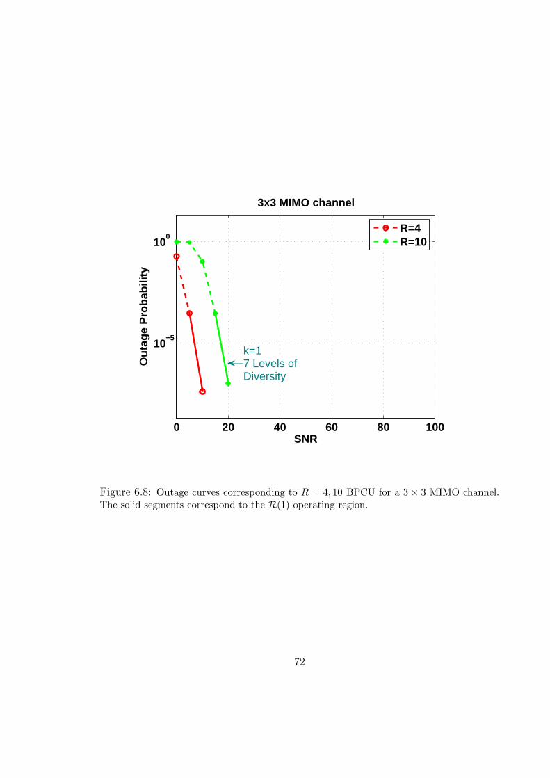
0 20 40 60 80 100
10−5
100
SNR
Out
age
Pro
babi
lity
3x3 MIMO channel
R=4R=10
k=17 Levels ofDiversity
Figure 6.8: Outage curves corresponding to R = 4, 10 BPCU for a 3 × 3 MIMO channel.The solid segments correspond to the R(1) operating region.
72
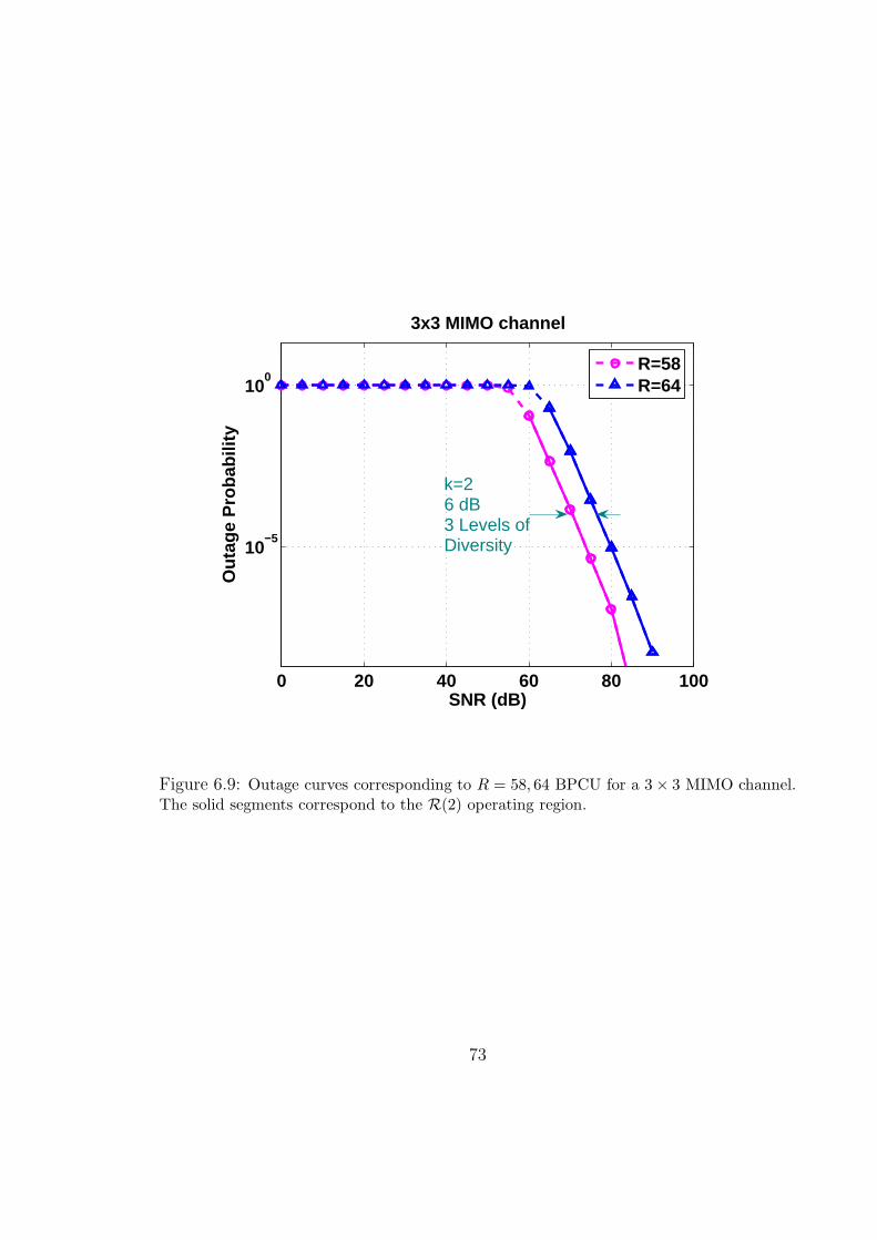
0 20 40 60 80 100
10−5
100
SNR (dB)
Out
age
Pro
babi
lity
3x3 MIMO channel
R=58R=64
k=26 dB3 Levels ofDiversity
Figure 6.9: Outage curves corresponding to R = 58, 64 BPCU for a 3 × 3 MIMO channel.The solid segments correspond to the R(2) operating region.
73
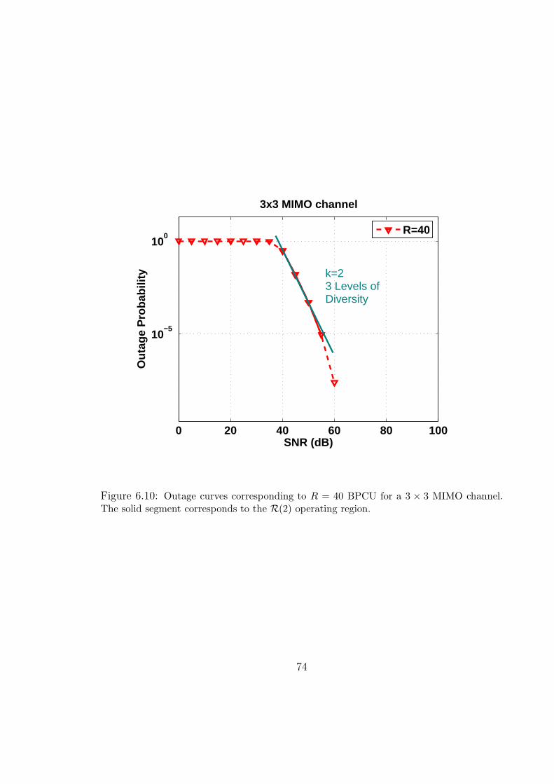
0 20 40 60 80 100
10−5
100
SNR (dB)
Out
age
Pro
babi
lity
3x3 MIMO channel
R=40
k=23 Levels ofDiversity
Figure 6.10: Outage curves corresponding to R = 40 BPCU for a 3 × 3 MIMO channel.The solid segment corresponds to the R(2) operating region.
74
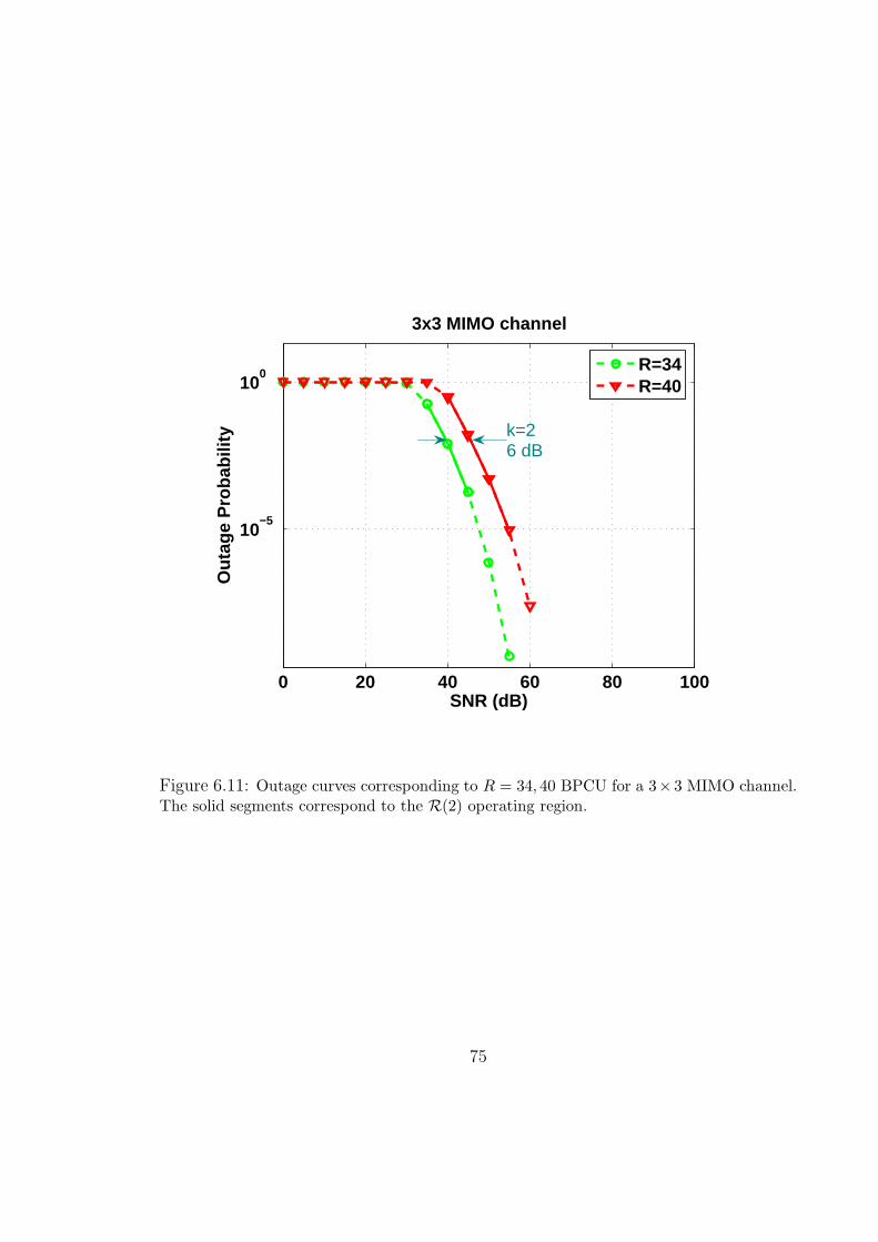
0 20 40 60 80 100
10−5
100
SNR (dB)
Out
age
Pro
babi
lity
3x3 MIMO channel
R=34R=40
k=26 dB
Figure 6.11: Outage curves corresponding to R = 34, 40 BPCU for a 3× 3 MIMO channel.The solid segments correspond to the R(2) operating region.
75
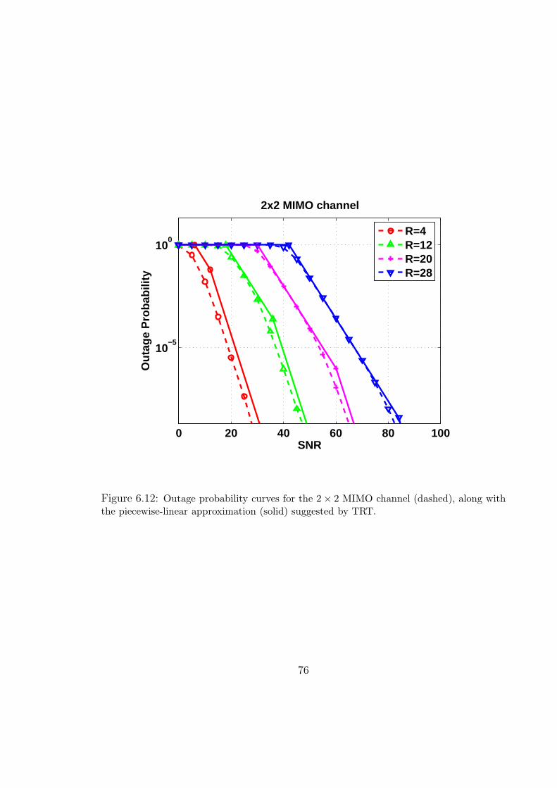
0 20 40 60 80 100
10−5
100
SNR
Out
age
Pro
babi
lity
2x2 MIMO channel
R=4R=12R=20R=28
Figure 6.12: Outage probability curves for the 2 × 2 MIMO channel (dashed), along withthe piecewise-linear approximation (solid) suggested by TRT.
76
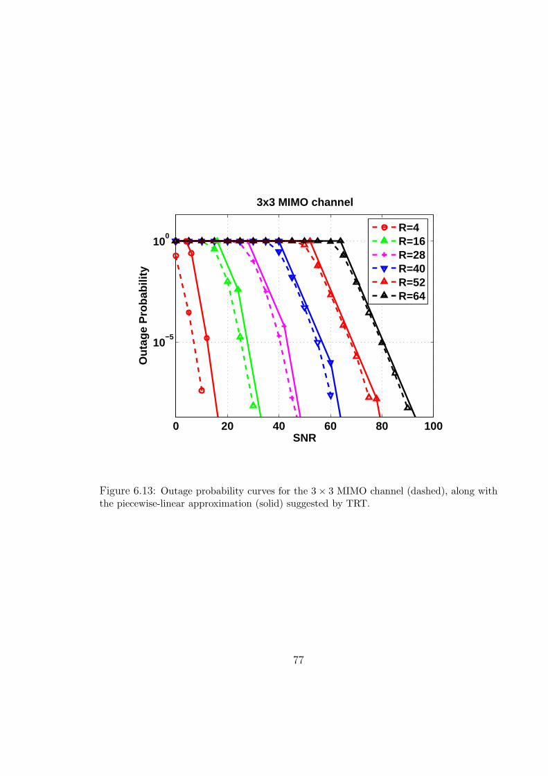
0 20 40 60 80 100
10−5
100
SNR
Out
age
Pro
babi
lity
3x3 MIMO channel
R=4R=16R=28R=40R=52R=64
Figure 6.13: Outage probability curves for the 3 × 3 MIMO channel (dashed), along withthe piecewise-linear approximation (solid) suggested by TRT.
77
where R(k), c(k), and g(k) are given by (6.5), (6.6), and (6.7), respectively. More-
over, there exists a coding scheme that achieves (6.17) for l ≥ m+ n− 1.
Proof : (Sketch) The proof follows the same lines as [17]. In particular, the converse
is obtained via a careful use of Fano’s inequality. The achievability is established
using an ensemble of Gaussian codebooks along with the appropriate use of the union
bound. Please refer to Appendix A.15 for a detailed proof.
One can also derive the TRT achievable by certain suboptimal space-time archi-
tectures. In this chapter, we restrict our study to square V-BLAST protocols and
orthogonal space-time constellations. In the V-BLAST architecture, the input stream
is split into m sub-streams. These sub-streams are then encoded independently and
transmitted over the m transmit antennas [26]. The following theorem character-
izes the throughput-reliability tradeoff for this protocol when a maximum likelihood
decoder is employed.
Theorem 18 The ML error probability for a V-BLAST communication system with
m transmit and m receive antennas satisfies8
limρ→ ∞R ∈ Rvb
logPe(R, ρ) −R
log ρ= −m, (6.18)
where Rvb is given by
Rvb , {R|m >R
log ρ> 0}.
Moreover, there exists a coding scheme that achieves (6.18) for l ≥ 2m− 1.
Proof : Please refer to the Appendix A.16.
8The subscript “vb” stands for V-BLAST.
78
Fig. 6.14 depicts the outage curves corresponding to R = 8 and 12 BPCU for
a 2 × 2 V-BLAST scheme with ML decoding. As can be seen from this figure, the
high SNR segments of the outage curves achieve 2 levels of diversity with a horizontal
spacing of 6 dB. These values agree with gvb(0) = 2 and tvb(0) = 2. Fig. 6.15, on
the other hand, compares the outage behavior of 2 × 2 MIMO and ML V-BLAST
schemes for R = 4, 16 and 32 BPCU. As can be seen from this figure, the outage
curves for the two schemes coincide while R/ log ρ > 1. In particular, the curves
corresponding to R = 32 BPCU are almost identical. However, for R/ log ρ < 1, the
sub-optimality of the V-BLAST becomes evident. In fact, the curve corresponding
to the 2 × 2 MIMO with R = 4 BPCU approaches 4 levels of diversity very rapidly,
while the curve corresponding to the V-BLAST only attains 2 levels.
Similarly, orthogonal space-time constellations allow for a simple TRT character-
ization. An orthogonal constellation of size m, length l, and rate k/l (in symbols per
channel use (spcu)) is a space-time code X ∈ Cm×l such that
XXH =
(k∑
i=1
|xi|2
)
× Im, (6.19)
where {xi}ki=1 denote the symbols to be sent, Im is the m ×m identity matrix and
XH denotes the hermitian of matrix X [27]. As an example, consider the orthogonal
constellation with m = 2, l = 2, and rate one, which is known as the Alamouti code
[28]. In this case
X =
[x1 −x∗2x2 x∗1
]
,
where x∗ denotes the complex conjugate of x. Notice that
XXH = (|x1|2 + |x2|
2) × I2,
79
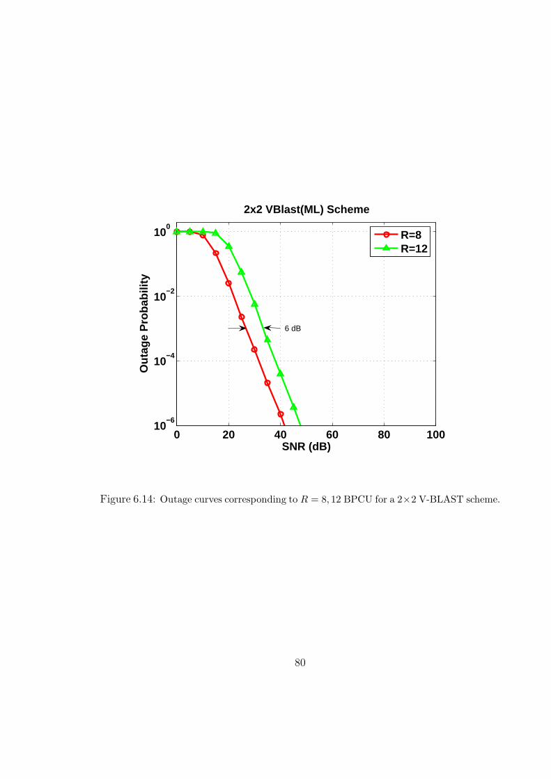
0 20 40 60 80 10010
−6
10−4
10−2
100
SNR (dB)
Out
age
Pro
babi
lity
2x2 VBlast(ML) Scheme
R=8R=12
6 dB
Figure 6.14: Outage curves corresponding to R = 8, 12 BPCU for a 2×2 V-BLAST scheme.
80
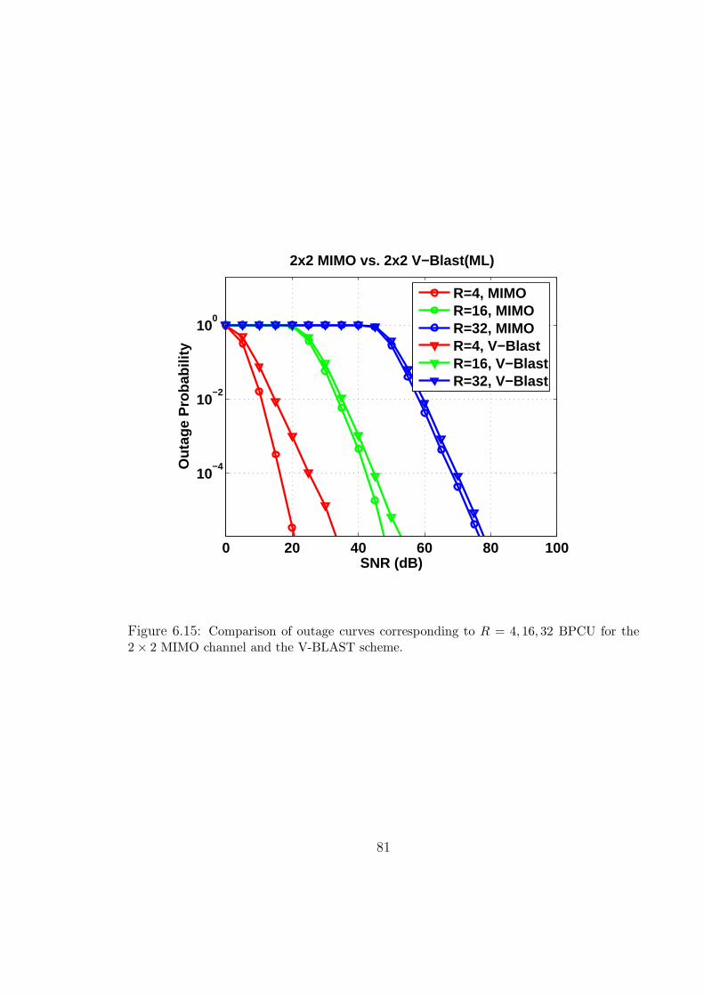
0 20 40 60 80 100
10−4
10−2
100
SNR (dB)
Out
age
Pro
babi
lity
2x2 MIMO vs. 2x2 V−Blast(ML)
R=4, MIMOR=16, MIMOR=32, MIMOR=4, V−BlastR=16, V−BlastR=32, V−Blast
Figure 6.15: Comparison of outage curves corresponding to R = 4, 16, 32 BPCU for the2 × 2 MIMO channel and the V-BLAST scheme.
81
as required by (6.19). The received signal matrix Y ∈ Cn×l at the destination can be
written as
Y =
√ρ
mHX + W. (6.20)
The ML receiver performs linear processing on Y to yield the following equivalent
parallel channel model
yi =
√ρ
m‖H‖2xi + wi, for i = 1, · · · , k. (6.21)
In (6.21), ‖H‖2 denotes the Frobenius norm of H (i.e., ‖H‖2 ,∑
|hij|2, where {hij}
are the entries of H) and {wi}ki=1 are i.i.d complex Gaussian random variables of
zero mean and unit variance. The following theorem gives the throughput-reliability
tradeoff for orthogonal constellations.
Theorem 19 The optimal throughput-reliability tradeoff for an orthogonal constella-
tion of size m, length l, rate k/l spcu (R BPCU) and n receive antennas satisfies9
limρ→ ∞R ∈ Roc
logPe(R, ρ) −lkmnR
log ρ= −mn, (6.22)
where Roc is given by
Roc , {R|k
l>
R
log ρ> 0},
Moreover, there exists an outer coding scheme (one that maps the information bits
into symbols {xi}ki=1) that achieves (6.22) for k ≥ mn.
Proof : The proof follows immediately from Theorem 17 and the fact that the
orthogonal constellation of interest effectively converts the underlying m× n MIMO
9The subscript “oc” stands for an orthogonal constellation.
82
channel of rate R (as given by (6.20)) into a 1 ×mn channel of rate lkR (as given by
(6.21)).
Fig. 6.16 depicts the outage curves corresponding to R = 4 and 8 BPCU for a
2×2 Alamouti scheme. As can be seen from this figure, the high SNR segments of the
outage curves achieve 4 levels of diversity with a horizontal spacing of 12 dB. These
values agree with goc(0) = 4 and toc(0) = 1. Fig. 6.17, on the other hand, compares
the outage behavior of the 2 × 2 MIMO channel and the Alamouti constellation for
R = 4, 16 and 32 BPCU. As can be seen from this figure, while the outage curves for
the two schemes coincide for small rates, the sub-optimality of the Alamouti scheme
becomes evident at higher values of R. In particular, the curves corresponding to
R = 4 BPCU are almost identical and for R = 32 BPCU the curve corresponding to
the Alamouti scheme lags that of MIMO by more than 40 dB.
Finally, we extend our analysis to MIMO-ARQ channels. In this setup, the trans-
mitter starts by picking up a message from the transmission buffer. It then uses a
space-time encoder to map the message to a sequence of blocks Xp ∈ Cm×l, L ≥ p ≥ 1.
During transmission-round p, the transmitter sends Xp one column at a time over its
m antennas. The receiver then tries to decode the message. If successful, it sends back
a positive acknowledgement signal (ACK), which causes the transmitter to start send-
ing the next message. However, if the receiver detects an error, it requests another
round of transmission by feeding back a negative acknowledgement signal (NACK).
The only exception to this rule is when L rounds of transmission have already been
sent, in which case the transmitter abandons sending the current message and goes to
the next one. In this chapter, we address the long-term static channel scenario, where
all of the transmission-rounds corresponding to a message take place over the same
83
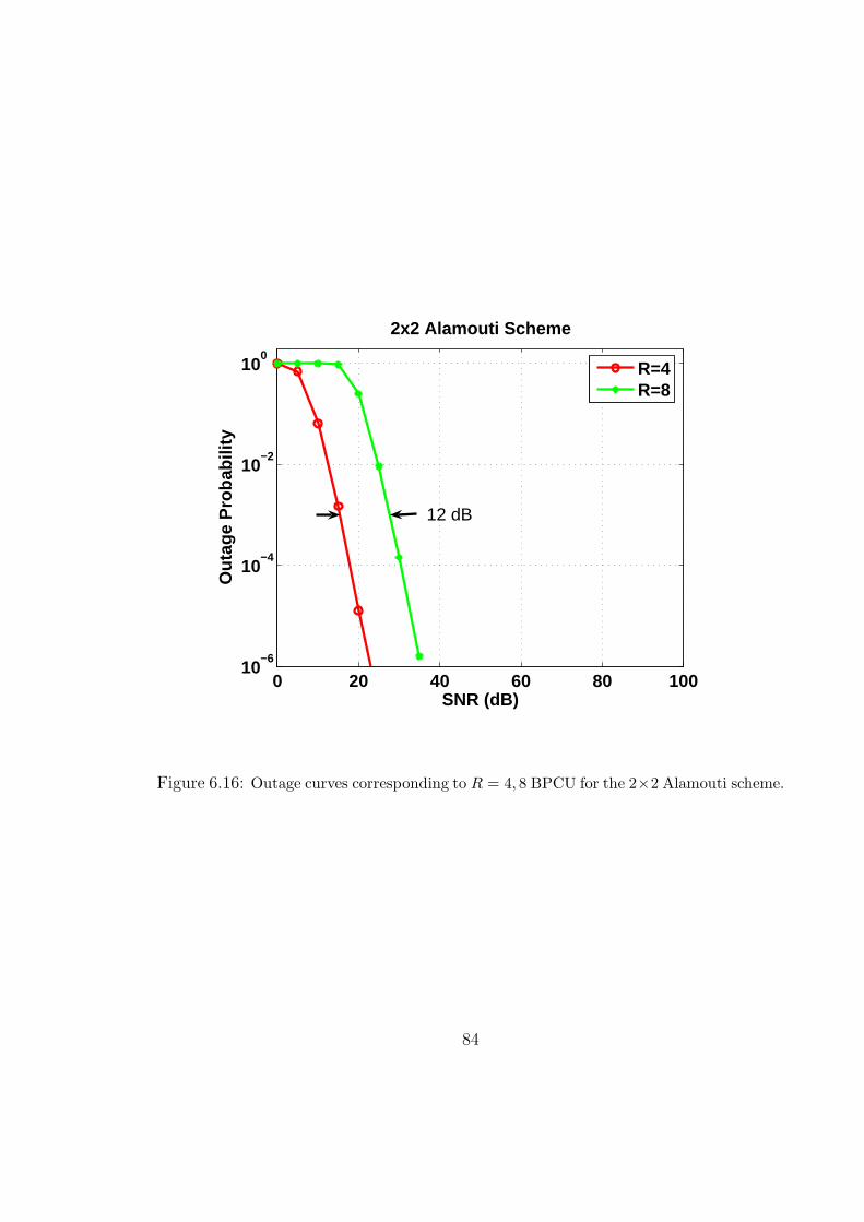
0 20 40 60 80 10010
−6
10−4
10−2
100
SNR (dB)
Out
age
Pro
babi
lity
2x2 Alamouti Scheme
R=4R=8
12 dB
Figure 6.16: Outage curves corresponding to R = 4, 8 BPCU for the 2×2 Alamouti scheme.
84
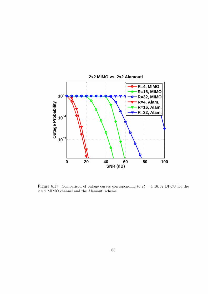
0 20 40 60 80 100
10−4
10−2
100
SNR (dB)
Out
age
Pro
babi
lity
2x2 MIMO vs. 2x2 Alamouti
R=4, MIMOR=16, MIMOR=32, MIMOR=4, Alam.R=16, Alam.R=32, Alam.
Figure 6.17: Comparison of outage curves corresponding to R = 4, 16, 32 BPCU for the2 × 2 MIMO channel and the Alamouti scheme.
85
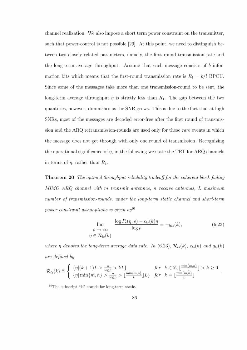
channel realization. We also impose a short term power constraint on the transmitter,
such that power-control is not possible [29]. At this point, we need to distinguish be-
tween two closely related parameters, namely, the first-round transmission rate and
the long-term average throughput. Assume that each message consists of b infor-
mation bits which means that the first-round transmission rate is R1 = b/l BPCU.
Since some of the messages take more than one transmission-round to be sent, the
long-term average throughput η is strictly less than R1. The gap between the two
quantities, however, diminishes as the SNR grows. This is due to the fact that at high
SNRs, most of the messages are decoded error-free after the first round of transmis-
sion and the ARQ retransmission-rounds are used only for those rare events in which
the message does not get through with only one round of transmission. Recognizing
the operational significance of η, in the following we state the TRT for ARQ channels
in terms of η, rather than R1.
Theorem 20 The optimal throughput-reliability tradeoff for the coherent block-fading
MIMO ARQ channel with m transmit antennas, n receive antennas, L maximum
number of transmission-rounds, under the long-term static channel and short-term
power constraint assumptions is given by10
limρ→ ∞
η ∈ Rls(k)
logPe(η, ρ) − cls(k)η
log ρ= −gls(k), (6.23)
where η denotes the long-term average data rate. In (6.23), Rls(k), cls(k) and gls(k)
are defined by
Rls(k) ,
{
{η|(k + 1)L > ηlog ρ
> kL} for k ∈ Z, ⌊min{m,n}L
⌋ > k ≥ 0
{η|min{m,n} > ηlog ρ
> ⌊min{m,n}L
⌋L} for k = ⌊min{m,n}L
⌋,
10The subscript “ls” stands for long-term static.
86
cls(k) ,c(k)
Land gls(k) , g(k),
respectively. c(k) and g(k) are given by (6.6) and (6.7).
Proof : (Sketch) The proof follows the same lines as that of Theorem 5 in [29].
In particular, the converse is obtained by lower-bounding the error probability of
the ARQ protocol with that of a ML decoder that operates on the whole codeword
{Xp}Lp=1. The achievability, on the other hand, is established through the use of an
ensemble of Gaussian code-books, along with a bounded-distance decoder. The main
idea here is to differentiate between the undetected-errors (i.e., the ones for which
the receiver sends back an ACK signal) and those errors that the decoder makes after
requesting L rounds of transmission. It can then be shown that, through judicious
choice of decoder threshold-distance, the latter error type becomes dominant, and
hence, the lower and upper bounds become tight. It is then straightforward to argue
the existence of codes in the ensemble that perform at least as well as the ensemble
average.
87
CHAPTER 7
CONCLUSIONS
We designed cooperation protocols for channels consisting of half-duplex nodes.
We considered relay, CB, MAR and CMA scenarios and devised protocols in each case.
We further demonstrated the gains and opportunities provided by ARQ techniques,
through presenting DDF variants for the ARQ relay, MAR and CVMA channels. We
evaluated the performance of the proposed protocols using DMT. We also presented a
new formulation for the throughput-reliability tradeoff in MIMO channels that avoids
the limitations imposed by the notion of multiplexing gain. In the sequel, we briefly
review the main contributions of this work and suggest a few directions for possible
future research.
7.1 Summary of Original Work
1. For the AF relay channel (single relay), we first established an upper bound on
the achievable DMT. We then proposed a nonorthogonal amplify and forward
(NAF) protocol that achieves this upper bound. Finally, we generalized the
NAF protocol to the case of arbitrary number of relays and characterized its
DMT. Notably, we showed that the NAF protocol outperforms the LW-STC
protocol without requiring decoding/encoding at the relays.
88
2. For the DF relay channel (single relay), we proposed a dynamic decode and
forward (DDF) protocol and proved its optimality (with respect to DMT), over
the range of multiplexing gains 1/2 ≥ r ≥ 0. Furthermore, we showed that the
DDF protocol outperforms all AF protocols at any multiplexing gain. Finally,
we extended the DDF protocol to the case of arbitrary number of relays and
characterized its tradeoff curve.
3. We presented a novel variant of the (single relay) DDF protocol, which is partic-
ularly suitable for implementation. In this variant, the channel seen by the des-
tination is reduced to a single-input single-output (SISO) time-selective channel.
Furthermore, to reduce the complexity of the protocol, we confined the relay
to start transmission only at the beginning of a finite number of segments. We
gave the rule for determining these segments such that the variant is Pareto
optimal with respect to DMT.
4. For the CB channel, we presented a variant of the DDF protocol that allows for
efficient transmission of common information. We then established the superi-
ority of this protocol, over AF protocols, by characterizing its tradeoff curve.
We also argued that the gain offered by the DDF protocol is more significant
in this scenario, as compared to the relay channel.
5. For the symmetric MAR channel (two users), we first derived an upper bound
on the achievable DMT. We then modified the DDF protocol to match it to
the MAR channel and derived its tradeoff curve. This characterization showed
that the DDF protocol is DMT optimal over the range of multiplexing gains
3/4 ≥ r ≥ 0. It also revealed that in the MAR channel, a single relay can be
89
utilized by several users to simultaneously improve the diversity gain achieved
by all of them.
6. For the symmetric CMA channel, we proposed a novel AF protocol where an
artificial inter-symbol interference (ISI) channel is created. We proved the opti-
mality (in terms of DMT) of this protocol by showing that, for all multiplexing
gains (i.e., 1 ≥ r ≥ 0), it achieves the DMT of the corresponding N × 1 MIMO
channel. We then used this result to argue that the sub-optimality of the pro-
tocols proposed in [3] is a consequence of using orthogonal sub-channels, rather
than the half-duplex constraint. We further utilized this result to elucidate the
fundamental difference between the relay and CMA channels.
7. For the ARQ relay and MAR (two-user) channels, we first modified the corre-
sponding DDF protocols to incorporate ACK/NACK feedback signals. We then
characterized their achieved tradeoff curves, which proved their optimality.
8. For the ARQ CVMA channel (two users and two receiving antennas), we de-
veloped a new variant of the DDF protocol where the users are purposefully
instructed not to cooperate in the first round of transmission. Lower and upper
bounds on the achievable DMT were then derived. These bounds were shown to
converge to the optimal tradeoff as the number of transmission rounds increases.
9. We identified the limitation imposed by the notion of multiplexing gain and
develop a new formulation for the throughput-reliability tradeoff that avoids
this limitation. In this formulation, the multiplexing gain notion is replaced by
the more general concept of operating regions.
90

10. We used the proposed TRT formulation to elucidate the asymptotic trends
exhibited by MIMO channels. In particular, we devised a piecewise linear ap-
proximation to the outage probability of MIMO channels (at fixed rates), which
becomes progressively more accurate as rate and SNR grow.
11. We characterized the TRT, along with the corresponding piecewise linear outage
approximation, for the V-BLAST, orthogonal constellations and ARQ MIMO
channels.
7.2 Possible Future Work
In the sequel we give a few directions for possible future research.
• Proving (or disproving) the optimality of the DDF protocol for the single relay
channel and r > 0.5 is an open problem.
• Generalizations of the proposed protocols to multi-antenna nodes, scenarios
with different QoS constraints, and asymmetric channels are of definite interest.
• Extension of the proposed protocols to the non-coherent scenario, where all or
part of CSI is not available to cooperating nodes and/or destination is very
important.
• Characterization of the performance degredation resulting from asynchronicities
among the cooperating partners is a rather valuable direction to follow.
• Design of practical coding/decoding strategies that approach the fundamental
limits achievable through Gaussian codes and maximum likelihood decoding is
an important venue to pursue [30, 31].
91

• The piecewaise-linear outage-probability approximation suggested by TRT gives
accurate predictions when the operating point is well within certain regions of
the rate-SNR plane. Characterization of the outage-probability in the transi-
tional regions remains an open problem.
• For MIMO channels, we established the correspondence between the DMT and
TRT formulations (refer to (6.8) and (6.9)). It remains to be seen if such a
correspondence exits for general channels or not.
92
APPENDIX A
PROOF OF THE THEOREMS
A.1 Proof of Lemma 1
For simplicity, we prove the lemma for the real AWGN channel (the complex
channel is a straightforward extension), i.e.
yk = hxk + nk for l ≥ k ≥ 1,
where yk is the received signal over the kth symbol-interval, h is the channel gain and
nk is the i.i.d. Gaussian noise sample during symbol-interval k. Next we characterize
the average error probability PE|h, where averaging is invoked with respected to the
ensemble of Gaussian codes, conditioned on a particular h (which is assumed to be
known at the decoder). Towards this end, we divide a codeword into N segments,
each consisting of T symbol-intervals, i.e. l = NT . In our analysis, we consider the
asymptotic scenario where N and T grow to infinity. The ML decoder waits for N ′
segments before it starts decoding, where N ′ is given by
N ′ =
⌊NR
I(xk; yk)
⌋
+ 1, (A.1)
In (A.1), I(xk; yk) denotes the mutual information between xk and yk. Notice that
assuming the data rate to be less than the channel capacity guarantees N ′ ≤ N . Also,
93

observe that the fraction of codeword that the decoder has to wait before decoding
satisfies
limN→∞
N ′
N=
R
I(xk; yk).
Our analysis is based on exactly the same techniques used to establish the achievabil-
ity of the AWGN channel capacity, i.e., we first upper-bound the ML error probability
with that of a typical set decoder and then take the average of the latter error prob-
ability, over the ensemble of random Gaussian code-books. In particular, following
exactly the same argument as in Theorem 10.1.1 in [25], we get
PE|h ≤ 2ǫ+ 23N ′Tǫ2−T (N ′I(xk;yk)−NR),
≤ 3ǫ,
for sufficiently large N and T . This follows from the choice of N ′ in (A.1). It is
important to note that the transmission rate R is constant, i.e., independent of h,
and N ′ is not known to the transmitter.
A.2 Proof of Theorem 2
Due to the source average energy constraint, setting A1 and A2 to anything other
than the identity matrix will reduce the mutual information between x and y. Since
we are interested in obtaining an upper bound, we will choose A1 = Il′ and A2 = Il−l′,
in which case (3.1) reduces to
y =
[g1Il′ 0g2hB g1Il−l′
]
x +
[0g2B
]
w + v. (A.2)
Using singular value decomposition (SVD), the matrix B can be factored as
B = UDV H ,
94
where U ∈ C(l−l′)×(l−l′) and V ∈ C
l′×l′ are unitary and where D ∈ C(l−l′)×l′ is non-
negative diagonal with the diagonal elements in decreasing order. Using these matri-
ces, we define y , Ty, x , Tx, v , Tv, and w , V Hw, for unitary transformation
T ,
[V H 00 UH
]
.
The unitary property of V and T implies that Σw = σ2wIl and Σv = σ2
vIl, as well as
I(x;y) = I(x; y). (A.3)
In terms of the new variables, (A.2) becomes
y =
[g1Il′ 0g2hD g1Il−l′
]
x +
[0g2D
]
w + v
=
[g1Il′ 0g2hD g1Il−l′
]
x + n (A.4)
with
Σn =
[σ2
vIl′ 00 σ2
vIl−l′ + |g2|2σ2
wDDH
]
.
If we denote the non-zero diagonal elements of D as {di}mi=1, then (A.4) can be written
as
yi = Gixi + ni, i = 1, . . . , m
yi = g1xi + ni, i = m+ 1, . . . , l′ and i = l′ +m+ 1, . . . , l,
where yi, xi and ni represent the ith element of y, x and n, respectively, and where
yi , [yi, yl′+i]t, xi , [xi, xl′+i]
t, ni , [ni, nl′+i]t, and
Gi ,
[g1 0
g2hdi g1
]
, (A.5)
Σni=
[σ2
v 00 σ2
v + |g2|2d2
iσ2w
]
. (A.6)
95
Note that, according to the SVD theorem,
m ≤ min{l′, l − l′}. (A.7)
Because Σn is diagonal, I(x; y) (and therefore I(x;y)) is maximized when {xi}mi=1 ∪
{xi}l′
i=m+1 ∪ {xi}li=l′+m+1 are mutually independent, in which case we would have
maxΣ
x
I(x; y) =m∑
i=1
maxΣ
xi
I(xi; yi) +l′∑
i=m+1
max I(xi; yi) +l∑
i=l′+m+1
max I(xi; yi). (A.8)
The mutual information between xi and yi is given by
I(xi; yi) = log(det (I2 + Σ− 1
2niGiΣxi
GHi Σ
− 12
ni)).
A lower-bound on maxΣxiI(xi; yi) is easily obtained by replacing Σxi
by EI2:
log(det (I2 + EGiGHi Σ−1
ni)) ≤ max
Σxi
I(xi; yi). (A.9)
Since log(det (.)) is an increasing function on the cone of positive-definite Hermitian
matrices and since λmaxI2 −Σxi≥ 0 (where λmax represents the largest eigenvalue of
Σx), we get the following upper-bound on maxΣxiI(xi; yi):
maxΣ
xi
I(xi; yi) ≤ log(det (I2 + λmaxGiGHi Σ−1
ni)). (A.10)
From (A.9) and (A.10), we conclude that
log(det (I2 + EGiGHi Σ−1
ni))
log(ρ)≤
maxΣxiI(xi; yi)
log(ρ)≤
log(det (I2 + λmaxGiGHi Σ−1
ni))
log(ρ).
Now, since λmax is of the same exponential order as E, the bounds converge as ρ
grows to infinity. That is
limρ→∞
maxΣxi
,diI(xi; yi)
log(ρ)= lim
ρ→∞
log(det (I2 + EGiGHi Σ−1
ni))
log(ρ).
96
Plugging in for Gi and Σnifrom (A.5) and (A.6), respectively, we get
limρ→∞
maxΣxi
,diI(xi; yi)
log(ρ)= lim
ρ→∞
1
log(ρ)log(1 +
|g1|2E
σ2v
+ · · ·
(|g1|2 + |g2|
2|h|2|di|2)E
σ2v + |g2|2d2
iσ2w
+|g1|
4E2
σ2v(σ
2v + |g2|2d2
iσ2w)
).
It is then straightforward to see that
limρ→∞
maxΣxi
,diI(xi; yi)
log(ρ)= (max{2(1 − v1), 1 − (v2 + u)})+, (A.11)
where v1, v2 and u are the exponential orders of 1/|g1|2, 1/|g2|
2 and 1/|h|2, respectively.
In deriving this expression, we have assumed that (v1, v2, u) ∈ R3+; as explained
earlier, we do not need to consider realizations in which v1, v2 or u are negative.
Similarly,
limρ→∞
max I(xi; yi)
log(ρ)= (1 − v1)
+,
which, together with (A.11), (A.3) and (A.8), results in:
limρ→∞
maxΣxI(x;y)
log(ρ)= (l − 2m)(1 − v1)
+ +m(max{2(1 − v1), 1 − (v2 + u)})+.
(A.12)
For the quasi-static fading setup, the outage event is defined as the set of channel
realizations for which the instantaneous capacity falls below the target data rate.
Thus, our outage event O becomes
O = {(v1, v2, u)|maxΣx
I(x,y) < lR}.
Letting R grow with ρ according to
R = r log(ρ),
97
and using (A.12), we conclude that, for large ρ,
O+ = {(v1, v2, u) ∈ R3+|(l − 2m)(1 − v1)
+ + · · ·
m(max{2(1 − v1), 1 − (v2 + u)})+ < rl}, (A.13)
and thus
PO(R)=ρ−do(r) for do(r) = inf(v1,v2,u)∈O+
(v1 + v2 + u). (A.14)
As Zheng and Tse have shown in Lemma 5 of [17], do(r) provides an upper-bound on
d∗(r) (i.e., the optimal diversity gain at multiplexing gain r):
d∗(r) ≤ do(r). (A.15)
From (A.13) and (A.14), it is easy to see that the right hand side of (A.15) is maxi-
mized when m is set to its maximum, which, according to (A.7), is min{l′, l−l′}. This
is the case when B is full-rank. On the other hand, min{l′, l− l′} itself is maximized
when l′ = l/2 (assuming an even codeword length l), which corresponds to B being
a square matrix. For this B, do(r) can be shown to take the value of the right hand
side of (3.3). This completes the proof.
A.3 Proof of Theorem 3
The proof closely follows that for the MIMO point-to point communication system
in [17]. In particular, we assume that the source uses a Gaussian random code-book
of codeword length l, where l is taken to be even, and data rate R, where R increases
with ρ according to
R = r log(ρ).
98
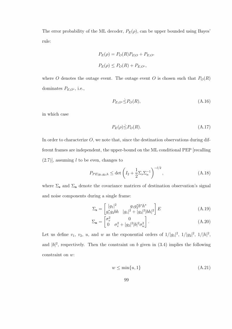
The error probability of the ML decoder, PE(ρ), can be upper bounded using Bayes’
rule:
PE(ρ) = PO(R)PE|O + PE,Oc
PE(ρ) ≤ PO(R) + PE,Oc,
where O denotes the outage event. The outage event O is chosen such that PO(R)
dominates PE,Oc, i.e.,
PE,Oc≤PO(R), (A.16)
in which case
PE(ρ)≤PO(R). (A.17)
In order to characterize O, we note that, since the destination observations during dif-
ferent frames are independent, the upper-bound on the ML conditional PEP [recalling
(2.7)], assuming l to be even, changes to
PPE|g1,g2,h ≤ det
(
I2 +1
2ΣsΣ
−1n
)−l/2
, (A.18)
where Σs and Σn denote the covariance matrices of destination observation’s signal
and noise components during a single frame:
Σs =
[|g1|
2 g1g∗2b
∗h∗
g∗1g2bh |g1|2 + |g2|
2|bh|2
]
E (A.19)
Σn =
[σ2
v 00 σ2
v + |g2|2|b|2σ2
w
]
. (A.20)
Let us define v1, v2, u, and w as the exponential orders of 1/|g1|2, 1/|g2|
2, 1/|h|2,
and |b|2, respectively. Then the constraint on b given in (3.4) implies the following
constraint on w:
w ≤ min{u, 1} (A.21)
99
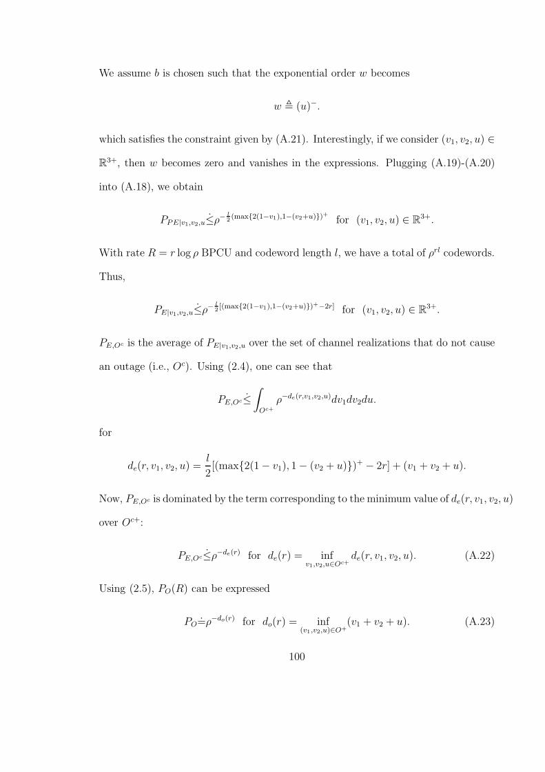
We assume b is chosen such that the exponential order w becomes
w , (u)−.
which satisfies the constraint given by (A.21). Interestingly, if we consider (v1, v2, u) ∈
R3+, then w becomes zero and vanishes in the expressions. Plugging (A.19)-(A.20)
into (A.18), we obtain
PPE|v1,v2,u≤ρ− l
2(max{2(1−v1),1−(v2+u)})+ for (v1, v2, u) ∈ R
3+.
With rate R = r log ρ BPCU and codeword length l, we have a total of ρrl codewords.
Thus,
PE|v1,v2,u≤ρ− l
2[(max{2(1−v1),1−(v2+u)})+−2r] for (v1, v2, u) ∈ R
3+.
PE,Oc is the average of PE|v1,v2,u over the set of channel realizations that do not cause
an outage (i.e., Oc). Using (2.4), one can see that
PE,Oc≤
∫
Oc+
ρ−de(r,v1,v2,u)dv1dv2du.
for
de(r, v1, v2, u) =l
2[(max{2(1 − v1), 1 − (v2 + u)})+ − 2r] + (v1 + v2 + u).
Now, PE,Oc is dominated by the term corresponding to the minimum value of de(r, v1, v2, u)
over Oc+:
PE,Oc≤ρ−de(r) for de(r) = infv1,v2,u∈Oc+
de(r, v1, v2, u). (A.22)
Using (2.5), PO(R) can be expressed
PO=ρ−do(r) for do(r) = inf(v1,v2,u)∈O+
(v1 + v2 + u). (A.23)
100
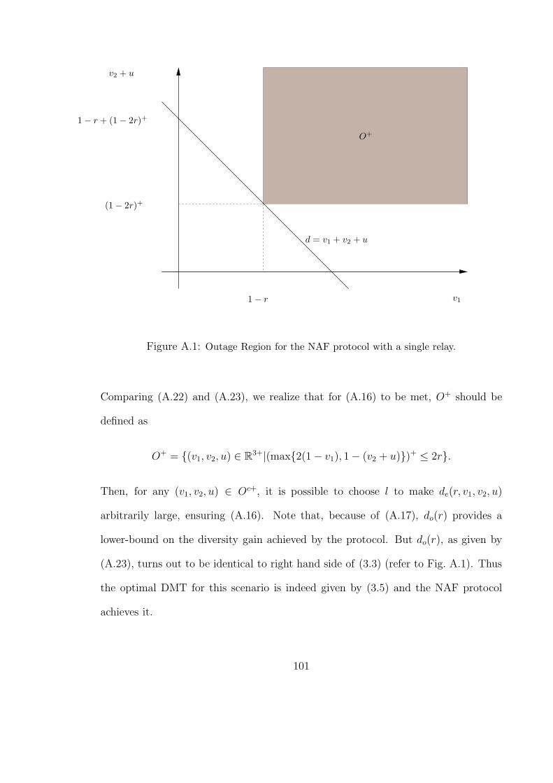
O+
v11 − r
(1 − 2r)+
1 − r + (1 − 2r)+
d = v1 + v2 + u
v2 + u
Figure A.1: Outage Region for the NAF protocol with a single relay.
Comparing (A.22) and (A.23), we realize that for (A.16) to be met, O+ should be
defined as
O+ = {(v1, v2, u) ∈ R3+|(max{2(1 − v1), 1 − (v2 + u)})+ ≤ 2r}.
Then, for any (v1, v2, u) ∈ Oc+, it is possible to choose l to make de(r, v1, v2, u)
arbitrarily large, ensuring (A.16). Note that, because of (A.17), do(r) provides a
lower-bound on the diversity gain achieved by the protocol. But do(r), as given by
(A.23), turns out to be identical to right hand side of (3.3) (refer to Fig. A.1). Thus
the optimal DMT for this scenario is indeed given by (3.5) and the NAF protocol
achieves it.
101

A.4 Proof of Theorem 5
Instead of considering specific codes, in the following we upper bound the average
probability of error over random Gaussian ensemble of code-books (employed by both
the source and relay). Therefore, averaging is invoked with respect to both, the fading
channel distribution and the random code-books. It is then straightforward to see
that there is at least one code-book in this ensemble whose average performance, now
with respect only to the fading channel distribution, is better than the predictions
of our upper bounds. For the single relay DDF protocol, the error probability of the
ML decoder, averaged over the ensemble of Gaussian code-books and conditioned on
a certain channel realization, can be upper bounded using Bayes’ rule to give
PE|g1,g2,h = PE,Ecr|g1,g2,h + PE,Er|g1,g2,h
PE|g1,g2,h ≤ PE|Ecr ,g1,g2,h + PEr|g1,g2,h,
where Er and Ecr denote the events that the relay decodes source’s message erro-
neously and its complement, respectively. The first step in the proof follows from
Lemma 1 by observing that if (3.6) is met, i.e., if the mutual information between the
signal transmitted by the source and the signal received by the relay exceeds lR, then
PEr|g1,g2,h can be made arbitrarily small, provided that the code-length is sufficiently
large. This means that for any ǫ > 0 and for a sufficiently large code-length,
PE|g1,g2,h < PE|Ecr,g1,g2,h + ǫ.
Taking the average over the ensemble of channel realizations gives
PE < PE|Ecr+ ǫ,
PE≤PE|Ecr.
102

This means that the exponential order of PE|Ecr, i.e., destination’s ML error probability
assuming error-free decoding at the relay, provides a lower-bound on the diversity gain
achieved by the protocol. Therefore, we only need to characterize PE|Ecr, which for
the sake of notational simplicity, we will denote by PE in the sequel. To characterize
PE, we note that the corresponding PEP [recalling (2.7)] is given by
PPE|g1,g2,h ≤
(
1 + |g1|2 E
2σ2v
)−l′ (
1 +(|g1|
2 + |g2|2) E
2σ2v
)−(l−l′)
. (A.24)
Defining v1, v2, and u as the exponential orders of 1/|g1|2, 1/|g2|
2, and 1/|h|2, respec-
tively, gives
PPE|v1,v2,u≤ρ−l[f(1−v1)++(1−f)(1−min{v1,v2})+] for (v1, v2, u) ∈ R
3+,
where f , l′/l. At a rate of R = r log ρ BPCU and a codeword length of l, there are
a total of ρrl codewords. Thus,
PE,Oc≤ρ−de(r)
for
de(r) = inf(v1,v2,u)∈Oc+
l[f(1 − v1)+ + (1 − f)(1 − min{v1, v2})
+ − r] + (v1 + v2 + u)
(A.25)
Examining (A.25), we realize that for (A.16) to hold, O+ should be defined as
O+ = {(v1, v2, u) ∈ R3+|f(1 − v1)
+ + (1 − f)(1 − min{v1, v2})+ ≤ r} (A.26)
so that it is possible to choose l to make de(r) arbitrarily large, ensuring (A.16). As
before, PO(R) is given by (A.23), which turns out to be identical to d(r) given by (3.7).
To see this, one needs to consider four different categories of channel realizations. The
103

first category is when both, v1 and v2 are greater than one. For this category,
inf(v1,v2,u)∈O+,
v1>1,v2>1
(v1 + v2 + u) = 2. (A.27)
The second category is when 1 ≥ v1 ≥ 0 and v2 > 1. It is easy to see from (A.26)
that for this category,
inf(v1,v2,u)∈O+,1≥v1≥0,v2>1
(v1 + v2 + u) = 2 − r. (A.28)
The third category to be considered is when v1 > 1 and 1 ≥ v2 ≥ 0. Before proceeding
further, note that from (3.6), one can show that
u = 1 −r
f. (A.29)
This implies that f ≥ r, since u is nonnegative. Returning back to (A.26), it is easy
to verify that for this category
v2 ≥ 1 −r
1 − f. (A.30)
Now, if f ≥ max{r, 1 − r}, then from (A.30) and (A.29) we get
inf(v1,v2,u)∈O+,v1>1,1≥v2≥0,f≥max{r,1−r}
(v1 + v2 + u) = inff≥max{r,1−r}
2 −r
f,
or
inf(v1,v2,u)∈O+,v1>1,1≥v2≥0,f≥max{r,1−r}
(v1 + v2 + u) =
{
1 + 1−2r1−r
, 12≥ r ≥ 0,
1, 1 ≥ r ≥ 12.
(A.31)
On the other hand, if 1 − r > f ≥ r, then
inf(v1,v2,u)∈O+,v1>1,1≥v2≥0,
1−r>f≥r
(v1 + v2 + u) = inf1−r>f≥r
3 −r
1 − f−r
f,
104
or
inf(v1,v2,u)∈O+,v1>1,1≥v2≥0,
1−r>f≥r
(v1 + v2 + u) = 1 +1 − 2r
1 − rfor
1
2> r ≥ 0.
This means that infO+(v1 + v2 + u), for the third category, is indeed given by (A.31).
It is noteworthy that the tradeoff curves given by (A.27), (A.28) and (A.31), are all
better than the genie-aided tradeoff. In other words, the diversity gain achieved by
this protocol is determined by the fourth category, where, both v1 and v2 are less
than or equal to one. For this category, one needs to consider two cases (Note that
(A.29) is still valid, implying f ≥ r). The first case, when 0.5 ≥ f ≥ r, is very easy.
Referring to Fig. A.2 reveals that, in this case, inf(v1,v2)∈O+ v1 +v2 and therefore do(r)
is equal to 2(1−r) (the genie aided tradeoff). The second case, when f > max{r, 0.5},
is a little bit more difficult. As can be seen from Fig. A.3, in this case
inf(v1,v2)∈O+
(v1 + v2) =1 − r
f. (A.32)
From (A.29) and (A.32), we conclude that
do(r) = inff>max{r,0.5}
1 +1 − 2r
f,
which gives (3.7). Again, according to (A.17), do(r) provides a lower-bound on the
diversity gain achieved by the protocol. On the other hand, do(r) is also an upper
bound on the achieved diversity since: 1) for 0 ≤ r ≤ 0.5 do(r) is the genie-aided
diversity and 2) for 0.5 ≤ r ≤ 1 it is easy to see that v1 = 1−rr
+ ǫ, v2 = 0 and u = 0
correspond to a channel outage for any ǫ > 0. Thus (3.7) is the diversity achieved by
the DDF protocol and the proof is complete.
105
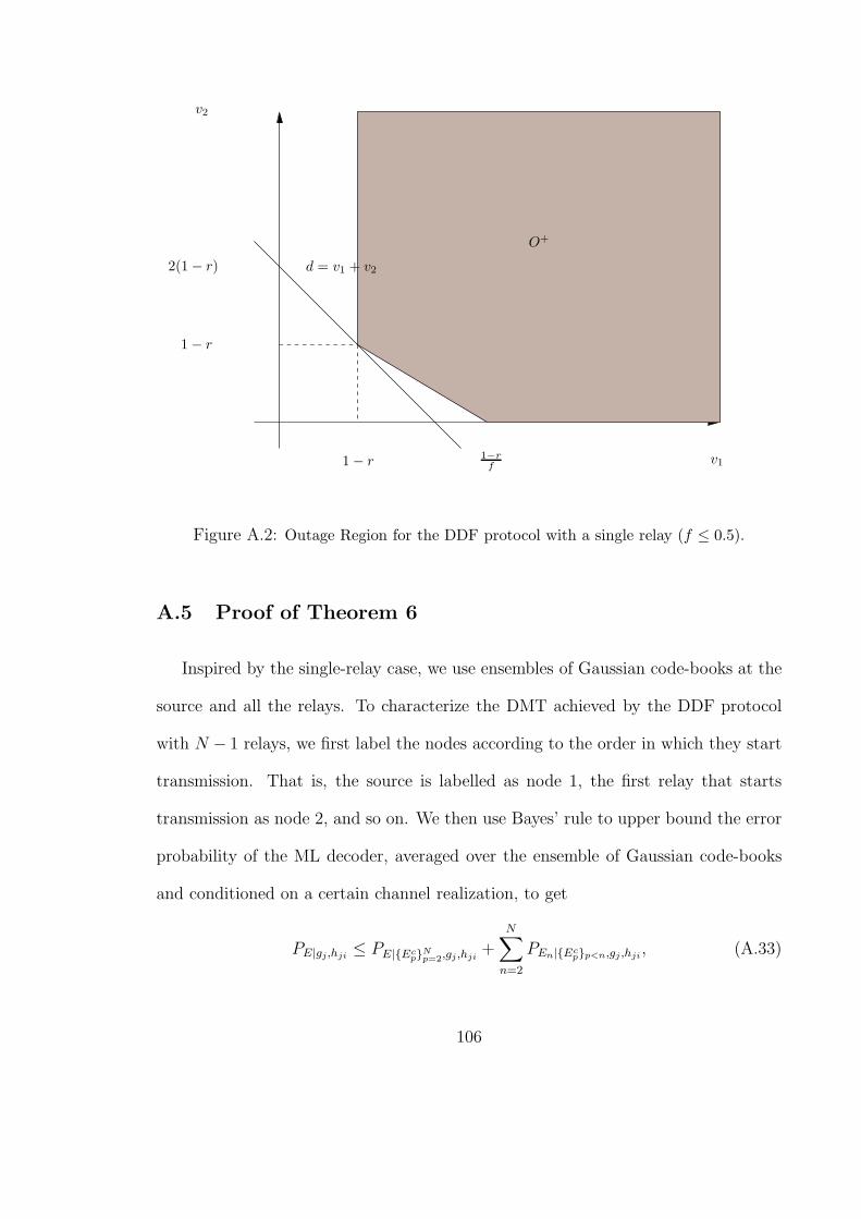
O+
v11−r
f1 − r
1 − r
d = v1 + v22(1 − r)
v2
Figure A.2: Outage Region for the DDF protocol with a single relay (f ≤ 0.5).
A.5 Proof of Theorem 6
Inspired by the single-relay case, we use ensembles of Gaussian code-books at the
source and all the relays. To characterize the DMT achieved by the DDF protocol
with N − 1 relays, we first label the nodes according to the order in which they start
transmission. That is, the source is labelled as node 1, the first relay that starts
transmission as node 2, and so on. We then use Bayes’ rule to upper bound the error
probability of the ML decoder, averaged over the ensemble of Gaussian code-books
and conditioned on a certain channel realization, to get
PE|gj,hji≤ PE|{Ec
p}Np=2,gj ,hji
+
N∑
n=2
PEn|{Ecp}p<n,gj ,hji
, (A.33)
106
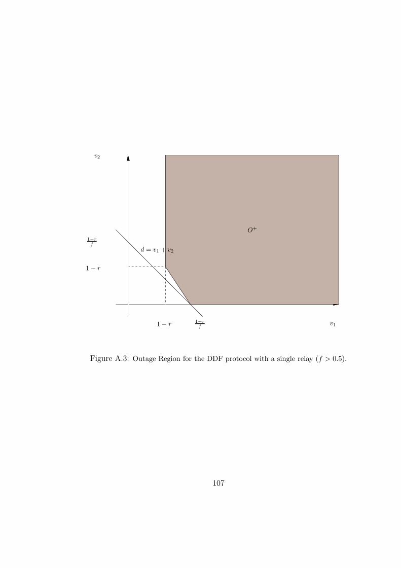
O+
v11−r
f1 − r
1 − r
1−rf
d = v1 + v2
v2
Figure A.3: Outage Region for the DDF protocol with a single relay (f > 0.5).
107
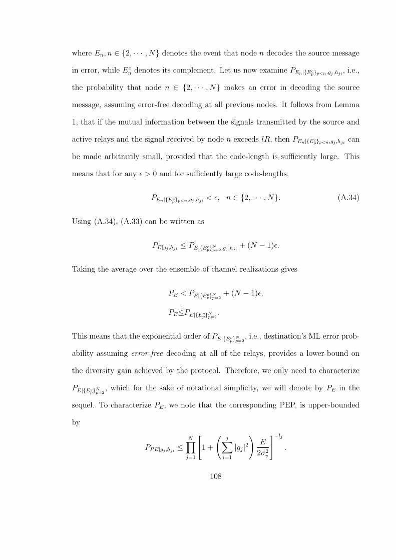
where En, n ∈ {2, · · · , N} denotes the event that node n decodes the source message
in error, while Ecn denotes its complement. Let us now examine PEn|{Ec
p}p<n,gj ,hji, i.e.,
the probability that node n ∈ {2, · · · , N} makes an error in decoding the source
message, assuming error-free decoding at all previous nodes. It follows from Lemma
1, that if the mutual information between the signals transmitted by the source and
active relays and the signal received by node n exceeds lR, then PEn|{Ecp}p<n,gj ,hji
can
be made arbitrarily small, provided that the code-length is sufficiently large. This
means that for any ǫ > 0 and for sufficiently large code-lengths,
PEn|{Ecp}p<n,gj ,hji
< ǫ, n ∈ {2, · · · , N}. (A.34)
Using (A.34), (A.33) can be written as
PE|gj,hji≤ PE|{Ec
p}Np=2,gj,hji
+ (N − 1)ǫ.
Taking the average over the ensemble of channel realizations gives
PE < PE|{Ecp}
Np=2
+ (N − 1)ǫ,
PE≤PE|{Ecp}
Np=2.
This means that the exponential order of PE|{Ecp}
Np=2
, i.e., destination’s ML error prob-
ability assuming error-free decoding at all of the relays, provides a lower-bound on
the diversity gain achieved by the protocol. Therefore, we only need to characterize
PE|{Ecp}
Np=2
, which for the sake of notational simplicity, we will denote by PE in the
sequel. To characterize PE, we note that the corresponding PEP, is upper-bounded
by
PPE|gj,hji≤
N∏
j=1
[
1 +
(j∑
i=1
|gj|2
)
E
2σ2v
]−lj
.
108
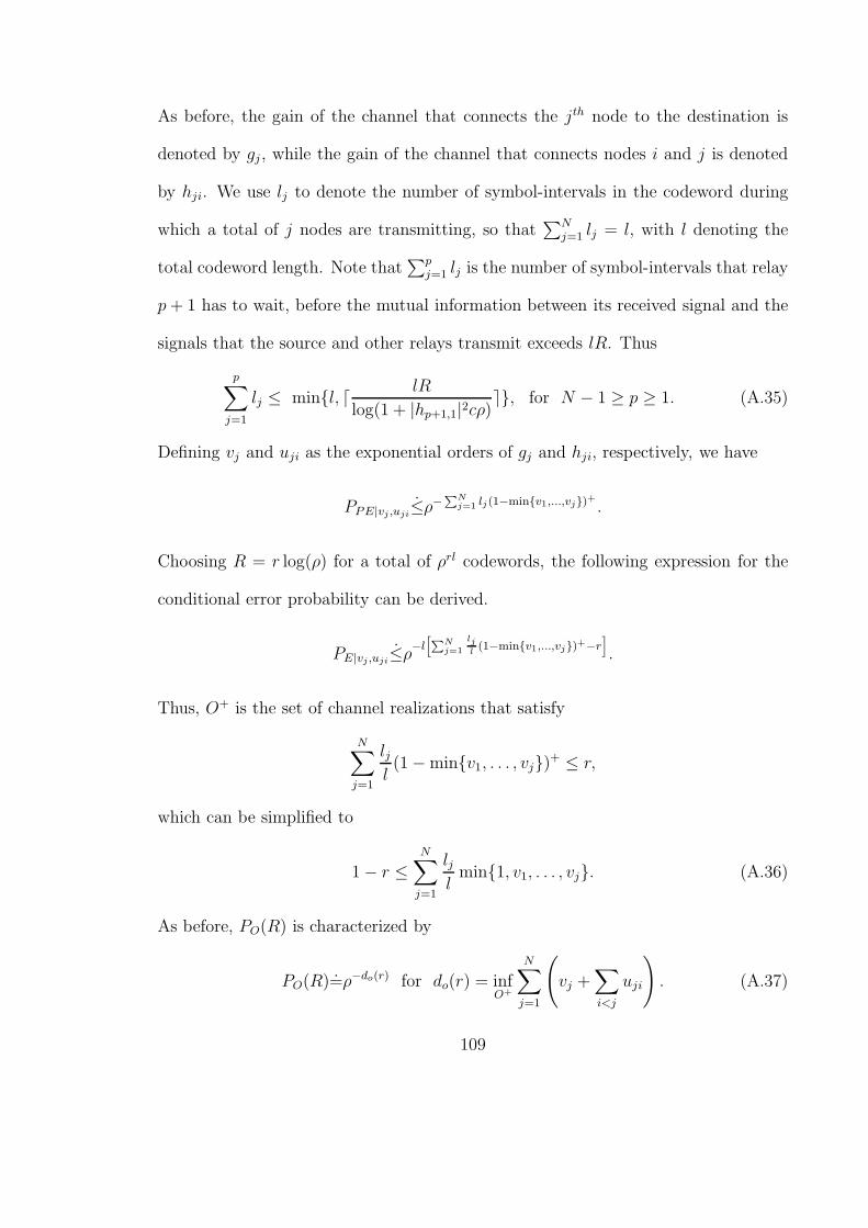
As before, the gain of the channel that connects the jth node to the destination is
denoted by gj , while the gain of the channel that connects nodes i and j is denoted
by hji. We use lj to denote the number of symbol-intervals in the codeword during
which a total of j nodes are transmitting, so that∑N
j=1 lj = l, with l denoting the
total codeword length. Note that∑p
j=1 lj is the number of symbol-intervals that relay
p+ 1 has to wait, before the mutual information between its received signal and the
signals that the source and other relays transmit exceeds lR. Thus
p∑
j=1
lj ≤ min{l, ⌈lR
log(1 + |hp+1,1|2cρ)⌉}, for N − 1 ≥ p ≥ 1. (A.35)
Defining vj and uji as the exponential orders of gj and hji, respectively, we have
PPE|vj ,uji≤ρ−
PNj=1 lj(1−min{v1,...,vj})+ .
Choosing R = r log(ρ) for a total of ρrl codewords, the following expression for the
conditional error probability can be derived.
PE|vj ,uji≤ρ
−lh
PNj=1
ljl(1−min{v1,...,vj})+−r
i
.
Thus, O+ is the set of channel realizations that satisfy
N∑
j=1
ljl(1 − min{v1, . . . , vj})
+ ≤ r,
which can be simplified to
1 − r ≤
N∑
j=1
ljl
min{1, v1, . . . , vj}. (A.36)
As before, PO(R) is characterized by
PO(R)=ρ−do(r) for do(r) = infO+
N∑
j=1
(
vj +∑
i<j
uji
)
. (A.37)
109

Defining vj , min{v1, · · · , vj}, j = 1, · · · , N lets us simplify (A.36) and (A.37) to
1 − r ≤
N∑
j=1
ljl
min{1, vj} (A.38)
do(r) ≥ infO+
N∑
j=1
(
vj +∑
i<j
uji
)
.
From the definition of vj, it follows that
v1 ≥ v2 ≥ · · · ≥ vN ≥ 0.
Note that (A.35) can also be simplified to
p∑
j=1
ljl≤ min
{
1,r
(1 − up+1,1)+
}
, for N − 1 ≥ p ≥ 1,
or
1 −r
∑pk=1
lkl
≤ uj1, for j > p. (A.39)
In order to characterize do(r), we need to consider three cases. The first case is
when 1 ≥ v1. In this case, (A.38) simplifies to
1 − r ≤
N∑
j=1
ljlvj.
Let us define xj , j(vj − vj+1), j = 1, · · · , N − 1 and xN , NvN . It immediately
follows that xj ≥ 0, j = 1, . . . , N . It is also easy to verify that
N∑
j=1
vj =N∑
j=1
xj and 1 − r ≤N∑
j=1
fj
jxj , (A.40)
where fj ,∑j
k=1 lk/l. From (A.40), it can be seen that
infO+
1≥v1
N∑
j=1
vj = p(1 − r
fp
)
, where p = arg maxN≥j≥1
{fj
j
}
. (A.41)
110
The infimum value corresponds to xp = p(1 − r)/fp and xj = 0, j 6= p or vj =
(1 − r)/fp, p ≥ j ≥ 1 and vj = 0, j > p. But we assumed 1 ≥ v1, so
fp ≥ 1 − r. (A.42)
From (A.39), it follows that,
infO+
1≥v1
∑
j>p
uj1 = (N − p)(1 −r
fp), 1 ≥ fp ≥ r. (A.43)
Now, from (A.41) and (A.43) we conclude that
infO+,1≥v1
N∑
j=1
(
vj +∑
i<j
uji
)
≥ infN≥p≥1,
1≥fp≥max{r,1−r}
do(r, p, fp),
where,
do(r, p, fp) , p(1 − r
fp) + (N − p)(1 −
r
fp). (A.44)
It turns out that, (A.44) is an increasing function of p. Therefore, its infimum corre-
sponds to p = 1. Now, examining do(r, 1, f1), i.e.,
do(r, 1, f1) = (1 − r
f1) + (N − 1)(1 −
r
f1),
we realize that, for 1/N ≥ r ≥ 0, it decreases with f1, thus its infimum corresponds
to f1 = 1. On the other hand, for 1 ≥ r ≥ 1/N , do(r, 1, f1) becomes an increasing
function of f1, which means that its infimum corresponds to f1 = max{r, 1 − r}, i.e.
infO+,1≥v1
N∑
j=1
(
vj +∑
i<j
uji
)
≥
N(1 − r), 1N
≥ r ≥ 0,
1 + (N−1)(1−2r)1−r
, 12≥ r ≥ 1
N,
1−rr, 1 ≥ r ≥ 1
2.
(A.45)
The second case to be considered is when vi > 1 ≥ vi+1, N−1 ≥ i ≥ 1. It immediately
follows that
infO+
vi>1≥vi+1
i∑
j=1
vj = i. (A.46)
111

In this case, (A.38) can be written as
1 − r − fi ≤
N∑
j=i+1
ljlvj . (A.47)
If fi ≥ 1 − r, then from (A.47), we get
infO+
vi>1≥vi+1,fi≥max{r,1−r}
N∑
j=i+1
vj = 0. (A.48)
On the other hand, from (A.39), it follows that,
infuj1≥1− r
fi,j>i
N∑
j=i+1
uj1 = (N − i)(1 −r
fi
), 1 ≥ fi ≥ r. (A.49)
Now, from (A.46), (A.48) and (A.49) one can see that
infO+,
vi>1≥vi+1,fi≥max{r,1−r}
N∑
j=1
(
vj +∑
i<j
uji
)
≥ infN−1≥i≥1,
1≥fi≥max{r,1−r}
do(r, i, fi),
with
do(r, i, fi) , i+ (N − i)(1 −r
fi).
The infimum of do(r, i, fi) corresponds to i = 1 and fi = max{r, 1 − r}, i.e.,
infO+,
vi>1≥vi+1,fi≥max{r,1−r}
N∑
j=1
(
vj +∑
i<j
uji
)
≥
{
1 + (N−1)(1−2r)1−r
, 12≥ r ≥ 0,
1, 1 ≥ r ≥ 12.
(A.50)
If fi < 1 − r, then the problem of finding inf∑N
j=i+1 vj reduces to the first case (i.e.,
1 ≥ v1). Specifically, inf∑N
j=i+1 vj is given by (A.41), with N − i, fp − fi, r + fi and
p− i substituting N , fp, r and p. Thus,
infO+,
vi>1≥vi+1,1−r>fi≥r
( N∑
j=i+1
vj
)
= (p− i)(1 − r − fi
fp − fi
)
, where p = arg maxN≥j≥i+1
{fj − fi
j − i
}
.
(A.51)
112
Note that (A.42) still holds. Derivation of inf∑N
j=1
∑
i<j uji follows from (A.39),
infuj1≥1− r
fk,j>k
N∑
j=1
∑
i<j
uji ≥ (p− i)(1 −r
fi
) + (N − p)(1 −r
fp
), with fp > fi ≥ r.
(A.52)
From (A.46), (A.51) and (A.52), we conclude that
infO+,
vi>1≥vi+1,1−r>fi≥r
N∑
j=1
(
vj +∑
i<j
uji
)
≥ infN≥p>i≥1,
1≥fp≥1−r>fi≥r
do(r, i, p, fi, fp), (A.53)
where,
do(r, i, p, fi, fp) , i+ (p− i)(1 − r − fi
fp − fi) + (p− i)(1 −
r
fi) + (N − p)(1 −
r
fp).
(A.54)
As can be seen from (A.54), do(r, i, p, fi, fp) is a linear, and therefore monotonic,
function of p. Thus, its infimum corresponds to either p = i+1 or p = N . Now if the
infimum indeed corresponds to p = i+ 1, by plugging in p = i into (A.54), we derive
a lower-bound on it. That is,
infN≥p>i≥1,
1≥fp≥1−r>fi≥r
do(r, i, p, fi, fp) ≥ infN>i≥1
1≥fp≥1−r
i+ (N − i)(1 −r
fp
).
or
infN≥p>i≥1,
1≥fp≥1−r>fi≥r
do(r, i, p, fi, fp) ≥ 1 + (N − 1)1 − 2r
1 − r, for
1
2> r ≥ 0. (A.55)
Choosing p = N , on the other hand, gives
do(r, i, N, fi, 1) = i+ (N − i)(2 −r
1 − fi−r
fi),
which has an infimum value, corresponding to i = 1 and fi = r or fi = 1−r, identical
to the right-hand side of (A.55). This means that
infN≥p>i≥1,
1≥fp≥1−r>fi≥r
do(r, i, p, fi, fp) = 1 + (N − 1)1 − 2r
1 − r, for
1
2> r ≥ 0. (A.56)
113
Now, from (A.56), (A.53) and (A.50), we conclude that
infO+,
vi>1≥vi+1
N∑
j=1
(
vj +∑
i<j
uji
)
≥
{
1 + (N−1)(1−2r)1−r
, 12≥ r ≥ 0,
1, 1 ≥ r ≥ 12.
(A.57)
The third case (i.e., vN > 1), is trivial
infO+,
vN >1
N∑
j=1
(
vj +∑
i<j
uji
)
≥ N. (A.58)
From (A.45), (A.57) and (A.58) we conclude that (3.8) provides a lower-bound on
the diversity gain achieved by the protocol. On the other hand, do(r) is also an upper
bound on the diversity since: 1) for 1/N ≥ r ≥ 0, do(r) is the genie-aided diversity, 2)
for 0.5 ≥ r ≥ 1/N , it can be shown that the realization, where v1 = 1+ǫ, {vj}Nj=2 = 0,
{uj1}Nj=2 = 1−2r
1−rand {uji}i6=j = 0 corresponds to a channel outage for any ǫ > 0, and
3) for 1 ≥ r ≥ 0.5, realization v1 = 1−rr
+ǫ, {vj}Nj=2 = 0 and {uji} = 0 also corresponds
to a channel outage for any ǫ > 0. Thus (3.8) is the diversity achieved by the N − 1
relay DDF protocol and the proof is complete.
A.6 Proof of Lemma 7
To prove the first part of the lemma, let us denote the signals received at the
destination by {yk}lk=1. Then
yk =
g1xk + vk for k = 1, · · · , l′
g1xk + g2x∗k+1 + vk for k = l′ + 1, l′ + 3, · · ·
g1xk − g2x∗k−1 + vk for k = l′ + 2, l′ + 4, · · ·
Now, through linear processing of {yk}lk=1, the destination derives {yk}
lk=1 such that
yk =
{g1xk + vk for k = 1, · · · , l′
√
|g1|2 + |g2|2xk + vk for k = l′ + 1, · · · , l, (A.59)
with vk being statistically identical to vk. Using (A.59), it is straightforward to see
that destination pairwise error probability, averaged over the ensemble of Gaussian
114
codes (used by the source) and conditioned on a certain channel realization, is still
given by (A.24). This means that modifying the DDF protocol according to (3.9)
does not effect the DMT achieved by the protocol.
To prove the second part, we notice that the effect of restricting the relay to start
transmission only after the codeword is halfway through, i.e., adopting (3.10) in place
of (3.6), is to replace (A.29) with
infO+,f
u =
{0 if f = 1
2
(1 − rf)+ if 1 ≥ f > 1
2
, (A.60)
where u denotes the exponential order of 1/|h|2. Now, since (A.60) is different from
(A.29) only for f = 1/2, for which inf(v1 + v2) is already equal to the optimal value
2(1 − r), we conclude that this restriction does not affect the DMT achieved by the
protocol.
A.7 Proof of Lemma 8
We notice that the outage set for the DDF protocol with a general set of waiting
fractions, {fj}Nj=1, is still given by (A.26), with the only difference that f is now given
by (compare with (A.29))
f =
f1 if 1 − rf1> u ≥ 0
fj if 1 − rfj> u ≥ (1 − r
fj−1)+
1 if u ≥ (1 − rfN
)+
. (A.61)
Next, we split O+ such that
O+ = ∪N+1j=1 O
+j , where O+
j = {(v1, v2, u) ∈ O+|f = fj}. (A.62)
Now, from (A.61) and (A.62) we get
infO+
j
u =
{0 for j = 1(1 − r
fj−1)+ for N + 1 ≥ j > 2
.
115

Also, since fj ≥12, we have inf(v1,v2)∈O+
j(v1 + v2) = (1 − r)/fj (recall (A.32)). Thus
dj(r) , infO+
j
(v1 + v2 + u),
dj(r) =1 − r
fj+ (1 −
r
fj−1)+. (A.63)
But, (A.62) along with (A.63) results in
d(r) = minfj≥r
dj(r),
d(r) = minfj≥r
1 − r
fj+ (1 −
r
fj−1)+. (A.64)
Now let us assume that the set of waiting fractions {fuj }
Nj=1 is uniformly optimal.
Pick {fj}Nj=1 such that fu
N < fN < 1. Then from (A.64) we conclude that for any
fuN < r < fN , du(r) = 1 − r and d(r) = 1 − r + 1 − r/fN . Thus du(r) < d(r), which
is in contradiction with the uniform optimality assumption of {fuj }
Nj=1. To prove the
second part of the lemma, we observe that for N ≥ j ≥ 1, {f pj }
Nj=1 as given by (3.11)
results in
dpN+1(r) < dp
j (r), for fj ≥ r ≥ 0, r 6= fj−1 (A.65)
and
dpN+1(fj−1) = dp
j(fj−1), or
dpN+1(fj−1) =
1 − fj−1
fj. (A.66)
Now (A.65), along with (A.64) and (A.63) proves that {f pj }
Nj=1 achieves (3.12). The
only thing left is to show that dp(r) is indeed Pareto optimal, i.e., no other set {fj}Nj=1
dominates {f pj }
Nj=1, in the Pareto sense. To do so, we assume such a set exists and
observe that since f0 = f p0 = 0 and fN+1 = f p
N+1 = 1, there should be N + 1 ≥ i ≥ 1
116

and N + 1 ≥ ℓ ≥ 1 such that
fi−1 ≤ f pℓ−1 < f p
ℓ < fi, or (A.67)
fi−1 < f pℓ−1 < f p
ℓ ≤ fi. (A.68)
Now, if (A.67) is true, then we observe from (A.64) that
d(f pℓ−1) ≤ di(f
pℓ−1) =
1 − f pℓ−1
fi<
1 − f pℓ−1
f pℓ
= dp(f pℓ−1),
where we have used (A.66) in deriving the last step. This, however is in contradiction
with the Pareto dominance of {fj}Nj=1, since
d(f pℓ−1) < dp(f p
ℓ−1).
On the other hand, if (A.68) is true, then
d(fi−1) ≤ di(fi−1) =1 − fi−1
fi< 2 − (1 +
1
f pN
)fi−1 = dp(fi−1),
or
d(fi−1) < dp(fi−1),
which again is in contradiction with Pareto dominance of {fj}Nj=1. This completes
the proof of the second part.
A.8 Proof of Theorem 9
To characterize the DMT achieved by the CB-DDF protocol, we first label the N
destinations according to the order in which they start transmission. That is, the first
destination that starts transmission is denoted as destination 1, the next destination
117
as destination 2, and so on. Note that the error probability of destination j can be
written as
PEj= PEj |Sc
jPSc
j+ PEj |Sj
PSj, (A.69)
where Sj denotes the event that destination j decodes the message and starts re-
transmission before the end of the codeword and Scj is its complement. Now, since
both PSjand PSc
jare less than one, (A.69) gives
PEj≤ PEj |Sc
j+ PEj |Sj
. (A.70)
In order to characterize PEj |Sj, we need to characterize PEj |Sj ,g,h, i.e., destination
j’s ML error probability, averaged over the ensemble of Gaussian code-books and
conditioned on a certain channel realization, under the assumption that it started
transmission before the end of the codeword. Towards this end and through using
Bayes’ rule, one can upper bound PEj |Sj ,g,h to get
PEj |Sj ,g,h ≤
j∑
i=1
PEi|{Ecp}p<i,Sj ,g,h. (A.71)
Now, let us examine PEi|{Ecp}p<i,Sj ,g,h, i.e., the probability that destination i (i ≤ j),
makes an error in decoding the source message, conditioned on Sj (which ensures that
destination i has indeed started re-transmission) and assuming error-free decoding at
all of the active destinations. It follows from Lemma 1, that if the mutual information
between the signals transmitted by the source and active destinations and the signal
received by destination i exceeds lR (which is implied by Sj), then PEi|{Ecp}p<i,Sj ,g,h
can be made arbitrarily small, provided that the code-length is sufficiently large. This
means that for any ǫ > 0 and for sufficiently large code-lengths,
PEi|{Ecp}p<i,Sj ,g,h < ǫ, i ≤ j. (A.72)
118
Using (A.72), (A.71) can be written as
PEj |Sj ,g,h ≤ jǫ.
Taking the average over the ensemble of channel realizations gives
PEj |Sj< jǫ.
This together with (A.70), yields
PEj< PEj |Sc
j+ jǫ,
PEj≤PEj |Sc
j. (A.73)
This means that the exponential order of PEj |Scj, provides a lower-bound on the di-
versity gain achieved by the protocol. Now, examining PEj |Scj, it is easy to realize
that the event in which the jth destination (out of N destinations), spends the entire
codeword listening, i.e. Scj , is identical to the DDF relay protocol with the rest of
the destinations taking the role of the N − 1 relays. Thus, from (A.73), we see that
communication to the jth destination achieves the same diversity order as does the
DDF relay protocol with N − 1 relays, namely, (4.1). This completes the proof.
A.9 Proof of Theorem 10
A simple max-cut min-flow examination reveals that the optimal diversity gain
for this channel is upper bounded by
dMAR(r) ≤ min{d3×1(r), d2×2(r), d2×1(r
2), d1×2(
r
2)}, (A.74)
where dm×n(·) denotes the optimal diversity gain for an m× n MIMO channel. Now,
(A.74) results in (4.2) and the proof of the converse part is complete.
119
In order to derive a lower bound on the diversity gain achieved by the DDF MAR
protocol, we upper bound the source-specific ML error probabilities, with that of the
joint ML decoder. Furthermore, instead of characterizing the latter probability for
specific codes, in the sequel, we characterize its average, PE , over the ensemble of
random Gaussian codes. It is then straightforward to see that there exists a code in
the ensemble, whose error probability is better than PE. To characterize PE, we use
the Bayes’ rule to derive the following upper bound
PE ≤ PE|Er+ PEr ,
where Er and Er denote the events that the relay makes errors in decoding the
messages, and its complement, respectively. Next, we note that if we denote the
signals transmitted by the two sources and the relay by {xj,k}lk=1 and {xr,k}
lk=l′+1 ,
respectively, and the signals received by the relay and the destination by {yr,k}l′
k=1 and
{yk}lk=1, then the number of symbol intervals l′ that the relay waits before decoding
the messages satisfies
lR
2≤ I({x1,k}
l′
k=1; {yr,k}l′
k=1|{x2,k}l′
k=1), (A.75)
lR
2≤ I({x2,k}
l′
k=1; {yr,k}l′
k=1|{x1,k}l′
k=1), (A.76)
lR ≤ I({x1,k}l′
k=1, {x2,k}l′
k=1; {yr,k}l′
k=1). (A.77)
In these expressions, R is the total data rate (in BPCU) at the destination and I(.; .)
denotes the mutual information function. Now, observing that (A.75), (A.76) and
(A.77) guarantee that (e.g., refer to section 14.3.1 of [25])
PEr ≤ ǫ, for any ǫ > 0,
120
we conclude
PE≤PE|Er.
For the sake of notational simplicity, in the sequel, PE|Eris denoted by PE . In
characterizing PE, we follow the approach of Tse, Viswanath and Zheng [18], by
partitioning the error event E into the set of partial error events EI , i.e.,
E =⋃
I
EI .
where I denotes any nonempty subset of {1, 2} and EI (referred to as type-I error)
is the event that the joint ML decoder incorrectly decodes the messages from sources
whose indices belong to I while correctly decoding all other messages. Because the
partial error events are mutually exclusive, we have
PE =∑
I
PEI. (A.78)
To characterize PEI, we use the Bayes’ rule to derive the following upper-bound
PEI= POI
PEI |OI+ PEI ,OI
PEI≤ POI
+ PEI ,OI,
where OI and OI denote the type-I outage event and its complement, respectively.
The type-I outage event is defined such that POIdominates PEI ,OI
, i.e.
PEI ,OI≤POI
. (A.79)
Thus,
PEI≤POI
. (A.80)
121
Characterization of OI , however, requires derivation of PPEI |g,h, i.e., the joint ML
decoder’s type-I pairwise error probability (PEP), conditioned on a particular chan-
nel realization and averaged over the ensemble of random Gaussian codes. For this
purpose, let us denote the gain of the channels connecting the two sources to the relay
by h1 and h2 and those of the channels connecting the two sources and the relay to
the destination by g1, g2 and gr, respectively. It is then straightforward to see that
(recall (2.7))
PPE{1}|g,h ≤ (1 +1
2ρ|g1|
2)−l′(1 +1
2ρ(|g1|
2 + |gr|2))−(l−l′),
PPE{1,2}|g,h ≤ (1 +1
2ρ(|g1|
2 + |g2|2))−l′(1 +
1
2ρ(|g1|
2 + |g2|2 + |gr|
2))−(l−l′).
Notice that since the channel is symmetric, PE{1}=PE{2}
, i.e., we do not need to
characterize PPE{2}|g,h. Let us denote the exponential orders of {1/|gj|2}2
j=1 and 1/|gr|2
by {vj}2j=1 and vr, respectively, and those of {1/|hj|
2}2j=1 by {uj}
2j=1. Realizing that,
at a rate of R = r log ρ BPCU and a codeword length of l, there are a total of ρlr
codewords in the code, we get
PE{1}|v,u≤ρ−l[f(1−v1)++(1−f)(1−min {v1,vr})+− r
2], (A.81)
PE{1,2}|v,u≤ρ−l[f(1−min {v1,v2})++(1−f)(1−min {v1,v2,vr})+−r], (A.82)
where f , l′/l. Careful examination of (A.81) reveals that defining O+{1} as
O+{1} , {(v1, · · · , u2) ∈ R
5+|f(1 − v1)+ + (1 − f)(1 − min{v1, vr})
+ ≤r
2}, (A.83)
satisfies (A.79). In this expression, O+{1} denotes O{1} ∩ R
5+, where Rn+ represents
the set of all nonnegative real n-tuples. This is because, if (A.83) is satisfied, then
through choosing a large enough l, PE{1},O{1}can be made arbitrarily small. Likewise,
122
defining O+{1,2} as
O+{1,2} ,
{(v1, · · · , u2) ∈ R5+|f(1 − min{v1, v2})
+ + (1 − f)(1 − min{v1, v2, vr})+ ≤ r},
(A.84)
satisfies (A.79). With the type-I outage events specified, the only thing left is to
characterize POI, i.e.
POI=ρ−dI(r) where dI(r) , inf
O+I
{v1 + v2 + vr + u1 + u2}. (A.85)
Toward this end, we use (A.83) to derive inf(v1,v2,vr)∈O+{1}
{v1 + v2 + vr}, as a function
of f , i.e.
inf(v1,v2,vr)∈O+
{1}
{v1 + v2 + vr}(f) = λ{1}(f),
where
λ{1}(f) ,
2 − r, 12> f ≥ 0
2 − r2(1−f)
, 1 − r2> f ≥ 1
22−r2f, 1 ≥ f ≥ 1 − r
2
(A.86)
Likewise, one can use (A.84) to derive
inf(v1,v2,vr)∈O+
{1,2}
{v1 + v2 + vr}(f) = λ{1,2}(f),
where
λ{1,2}(f) ,
3(1 − r), 23> f ≥ 0
3 − r1−f
, 1 − r > f ≥ 23
21−rf, 1 ≥ f ≥ 1 − r
, if1
3> r ≥ 0 (A.87)
or
λ{1,2}(f) ,
{3(1 − r), 2
3> f ≥ 0
21−rf, 1 ≥ f ≥ 2
3
, if 1 ≥ r ≥1
3(A.88)
123
Now, to complete the derivation of dI(r), we need to characterize inf(u1,u2)∈R2+{u1 +
u2}(f). For this purpose, we use (A.75), (A.76) and (A.77) to derive
l′ = min{l,max{⌈lR
2 log2 (1 + min{|h1|2, |h2|2}cρ)⌉, ⌈
lR
log2 (1 + (|h1|2 + |h2|2)cρ)⌉}},
where c is the ratio of destination noise variance to that of the relay and ⌈x⌉ denotes
the closest integer to x towards plus infinity. In terms of channel exponential orders,
this last expression can be rewritten as
f =min {1,max {r
2(1 − max {u1, u2})+,
r
(1 − min {u1, u2})+}}, (u1, u2) ∈ R
2+.
(A.89)
Now, using (A.89), one can show that
inf(u1,u2)∈R2+
{u1 + u2}(f) = λ(f),
where
λ(f) ,
{2(1 − r
f), 3r
2> f ≥ r
1 − r2f, 1 ≥ f ≥ 3r
2
. (A.90)
Using (A.85) we conclude
d{1}(r) = inff{λ(f) + λ{1}(f)},
which can be characterized using (A.86) and (A.90),
d{1}(r) =
2 − r, 12> r ≥ 0
4−5r2(1−r)
, 23≥ r ≥ 1
22−r2r, 1 ≥ r ≥ 2
3
. (A.91)
Similarly,
d{1,2}(r) = inff{λ(f) + λ{1,2}(f)},
124
which can be derived using (A.87), (A.88) and (A.90),
d{1,2}(r) =
{3(1 − r), 2
3> r ≥ 0
21−rr, 1 ≥ r ≥ 2
3
. (A.92)
Now, (A.91) and (A.92), together with (A.85), (A.80) and (A.78), result in (4.3) and
thus complete the proof of the achievability part.
A.10 Proof of Theorem 11
Realizing that (4.7) also corresponds to the optimal DMT for a MIMO point-to-
point communication system with N transmit antennas and a single receive antenna
(i.e., the case of “genie-aided” cooperation between N sources), we only need to show
that the CMA-NAF protocol achieves this tradeoff. To achieve this goal, we assume
that each of the sources uses a Gaussian random code with codeword length l and
data rate R, where l is chosen as in (4.5) and R grows with ρ according to (4.6).
We then characterize the joint ML decoder’s error probability PE(ρ). Note that the
error probability of the joint ML decoder upper-bounds the error probabilities of the
source-specific ML decoders and thus provides a lower-bound on the achievable overall
diversity gain (as a function of r). In characterizing PE(ρ), we follow the approach
of Tse et al. [18] by partitioning the error event E into the set of partial error events
{EI}, i.e.,
E =⋃
I
EI ,
where I denotes any nonempty subset of {1, ..., N} and EI (referred to as a ”type-
I error”) is the event that the joint ML decoder incorrectly decodes the messages
from sources whose indices belong to I while correctly decoding all other messages.
125
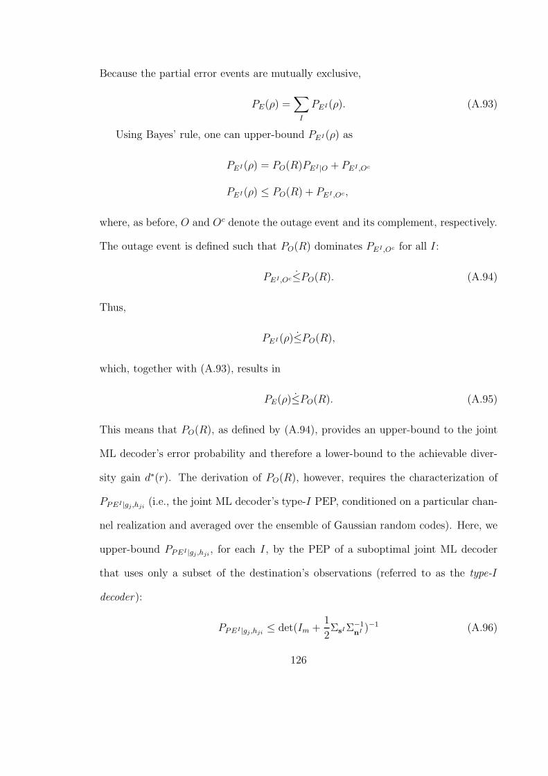
Because the partial error events are mutually exclusive,
PE(ρ) =∑
I
PEI(ρ). (A.93)
Using Bayes’ rule, one can upper-bound PEI(ρ) as
PEI(ρ) = PO(R)PEI |O + PEI ,Oc
PEI(ρ) ≤ PO(R) + PEI ,Oc,
where, as before, O and Oc denote the outage event and its complement, respectively.
The outage event is defined such that PO(R) dominates PEI ,Oc for all I:
PEI ,Oc≤PO(R). (A.94)
Thus,
PEI (ρ)≤PO(R),
which, together with (A.93), results in
PE(ρ)≤PO(R). (A.95)
This means that PO(R), as defined by (A.94), provides an upper-bound to the joint
ML decoder’s error probability and therefore a lower-bound to the achievable diver-
sity gain d∗(r). The derivation of PO(R), however, requires the characterization of
PPEI |gj ,hji(i.e., the joint ML decoder’s type-I PEP, conditioned on a particular chan-
nel realization and averaged over the ensemble of Gaussian random codes). Here, we
upper-bound PPEI |gj ,hji, for each I, by the PEP of a suboptimal joint ML decoder
that uses only a subset of the destination’s observations (referred to as the type-I
decoder):
PPEI |gj,hji≤ det(Im +
1
2ΣsI Σ−1
nI )−1 (A.96)
126
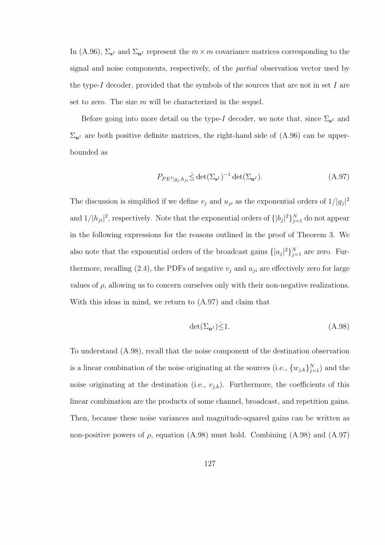
In (A.96), ΣsI and ΣnI represent the m×m covariance matrices corresponding to the
signal and noise components, respectively, of the partial observation vector used by
the type-I decoder, provided that the symbols of the sources that are not in set I are
set to zero. The size m will be characterized in the sequel.
Before going into more detail on the type-I decoder, we note that, since ΣsI and
ΣnI are both positive definite matrices, the right-hand side of (A.96) can be upper-
bounded as
PPEI |gj,hji≤ det(ΣsI )−1 det(ΣnI ). (A.97)
The discussion is simplified if we define vj and uji as the exponential orders of 1/|gj|2
and 1/|hji|2, respectively. Note that the exponential orders of {|bj |
2}Nj=1 do not appear
in the following expressions for the reasons outlined in the proof of Theorem 3. We
also note that the exponential orders of the broadcast gains {|aj|2}N
j=1 are zero. Fur-
thermore, recalling (2.4), the PDFs of negative vj and uji are effectively zero for large
values of ρ, allowing us to concern ourselves only with their non-negative realizations.
With this ideas in mind, we return to (A.97) and claim that
det(ΣnI )≤1. (A.98)
To understand (A.98), recall that the noise component of the destination observation
is a linear combination of the noise originating at the sources (i.e., {wj,k}Nj=1) and the
noise originating at the destination (i.e., vj,k). Furthermore, the coefficients of this
linear combination are the products of some channel, broadcast, and repetition gains.
Then, because these noise variances and magnitude-squared gains can be written as
non-positive powers of ρ, equation (A.98) must hold. Combining (A.98) and (A.97)
127
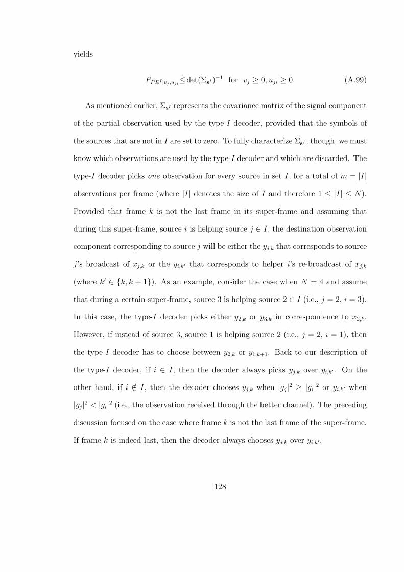
yields
PPEI |vj ,uji≤ det(ΣsI )−1 for vj ≥ 0, uji ≥ 0. (A.99)
As mentioned earlier, ΣsI represents the covariance matrix of the signal component
of the partial observation used by the type-I decoder, provided that the symbols of
the sources that are not in I are set to zero. To fully characterize ΣsI , though, we must
know which observations are used by the type-I decoder and which are discarded. The
type-I decoder picks one observation for every source in set I, for a total of m = |I|
observations per frame (where |I| denotes the size of I and therefore 1 ≤ |I| ≤ N).
Provided that frame k is not the last frame in its super-frame and assuming that
during this super-frame, source i is helping source j ∈ I, the destination observation
component corresponding to source j will be either the yj,k that corresponds to source
j’s broadcast of xj,k or the yi,k′ that corresponds to helper i’s re-broadcast of xj,k
(where k′ ∈ {k, k + 1}). As an example, consider the case when N = 4 and assume
that during a certain super-frame, source 3 is helping source 2 ∈ I (i.e., j = 2, i = 3).
In this case, the type-I decoder picks either y2,k or y3,k in correspondence to x2,k.
However, if instead of source 3, source 1 is helping source 2 (i.e., j = 2, i = 1), then
the type-I decoder has to choose between y2,k or y1,k+1. Back to our description of
the type-I decoder, if i ∈ I, then the decoder always picks yj,k over yi,k′. On the
other hand, if i /∈ I, then the decoder chooses yj,k when |gj|2 ≥ |gi|
2 or yi,k′ when
|gj|2 < |gi|
2 (i.e., the observation received through the better channel). The preceding
discussion focused on the case where frame k is not the last frame of the super-frame.
If frame k is indeed last, then the decoder always chooses yj,k over yi,k′.
128
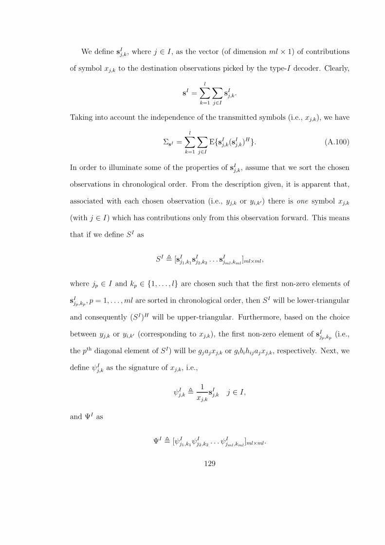
We define sIj,k, where j ∈ I, as the vector (of dimension ml × 1) of contributions
of symbol xj,k to the destination observations picked by the type-I decoder. Clearly,
sI =
l∑
k=1
∑
j∈I
sIj,k.
Taking into account the independence of the transmitted symbols (i.e., xj,k), we have
ΣsI =
l∑
k=1
∑
j∈I
E{sIj,k(s
Ij,k)
H}. (A.100)
In order to illuminate some of the properties of sIj,k, assume that we sort the chosen
observations in chronological order. From the description given, it is apparent that,
associated with each chosen observation (i.e., yj,k or yi,k′) there is one symbol xj,k
(with j ∈ I) which has contributions only from this observation forward. This means
that if we define SI as
SI , [sIj1,k1
sIj2,k2
. . . sIjml,kml
]ml×ml,
where jp ∈ I and kp ∈ {1, . . . , l} are chosen such that the first non-zero elements of
sIjp,kp
, p = 1, . . . , ml are sorted in chronological order, then SI will be lower-triangular
and consequently (SI)H will be upper-triangular. Furthermore, based on the choice
between yj,k or yi,k′ (corresponding to xj,k), the first non-zero element of sIjp,kp
(i.e.,
the pth diagonal element of SI) will be gjajxj,k or gibihijajxj,k, respectively. Next, we
define ψIj,k as the signature of xj,k, i.e.,
ψIj,k ,
1
xj,k
sIj,k j ∈ I,
and ΨI as
ΨI , [ψIj1,k1
ψIj2,k2
. . . ψIjml,kml
]ml×ml.
129

It follows then, that ΨI is also lower-triangular with the pth diagonal element being
equal to gjaj or gibihijaj. Using these definitions, (A.100) can be written as
ΣsI = E
l∑
k=1
∑
j∈I
ψIj,k(ψ
Ij,k)
H . (A.101)
The significance of ΨI can now be seen from the fact that (A.101) can be written as
ΣsI = EΨI(ΨI)H .
Now, as the determinant of triangular matrices is simply the product of their diagonal
elements, from (A.99) we conclude that
PPEI |vj ,uji≤ρ−m(N−1)L+
P
j∈I
[(m−1)Lvj+
P
i/∈I
(min{vj ,uji+vi}(L−1)+vj
)]
, vj ≥ 0, uji ≥ 0.
It is obvious that for large L’s, the previous inequality can be rewritten as
PPEI |vj ,uji≤ρ−
[−
P
j∈I
((m−1)vj+
P
i/∈I min{vj ,uji+vi})+m(N−1)
]L, vj ≥ 0, uji ≥ 0. (A.102)
At rate R = r log(ρ) and codeword length l, and when the symbols of the sources
that are not in I are set to zero, there are a total of ρm(N−1)Lr unique codewords.
Thus,
PEI |vj ,uji≤ρ−
[−
P
j∈I
((m−1)vj+
P
i/∈I min{vj ,uji+vi})+m(N−1)(1−r)
]L, vj ≥ 0, uji ≥ 0.
(A.103)
This conditional type-I error probability leads to
PEI ,Oc≤ρ−deI (r),
where
deI (r) , minO+
c
∑
j
(
vj +∑
i
uji
)
+ · · ·
[
−∑
j∈I
(
(m− 1)vj +∑
i/∈I
min{vj, uji + vi}
)
+m(N − 1)(1 − r)
]
L
(A.104)
130
Examining (A.104), we realize that for (A.94) to be met, O+ should be defined as
the set of all real N(N+1)2
-tuples with nonnegative elements that satisfy the following
condition for at least one nonempty I ⊆ {1, . . . , N}:
∑
j∈I
(
(m− 1)vj +∑
i/∈I
min{vj, vi + uji}
)
≥ m(N − 1)(1 − r) (A.105)
This way, by choosing large enough l, deI(r) can be made arbitrary large and thus
(A.94) is always met. From (A.105), it follows that
∑
j∈I
(
(m− 1)vj +∑
i/∈I
min{vj, vi + maxj 6=i
{uji}}
)
≥ m(N − 1)(1 − r). (A.106)
Substituting min{vj , vi + maxj 6=i{uji}} in this expression by vj gives
∑
j∈I
vj ≥ m(1 − r). (A.107)
On the other hand, replacing min{vj , vi+maxj 6=i{uji}} in (A.106) by vi+maxj 6=i{uji}
results in
(m− 1)∑
j∈I
vj +m∑
i/∈I
(vi + maxj 6=i
{uji}) ≥ m(N − 1)(1 − r). (A.108)
Under the constraints given by (A.107) and (A.108), it is easy to see that
infO+
(∑
j∈I
vj +∑
i/∈I
(vi + maxj 6=i
{uji})
)
≥ N(1 − r). (A.109)
Now, from (A.109) and (A.37), it follows that
do(r) ≥ N(1 − r).
Again, according to (A.95), do(r) provides a lower-bound on the diversity gain achieved
by the protocol. Thus the protocol achieves the diversity gain given by (4.7) and the
proof is complete.
131
A.11 Proof of Lemma 12
A simple min-cut max-flow examination reveals that the optimal diversity gain for
this channel is upper bounded by those of the 2× 1 and 1× 2 ARQ MIMO channels,
thus
dR(re, L) ≤ 2(1 −re
L) for 1 > re ≥ 0. (A.110)
Next we prove the achievability of this upper bound, by characterizing the DMT
for the proposed ARQ-DDF relay protocol. We do this in two steps. First, we
construct an ensemble of random Gaussian codes and characterize its average error
probability PE , and throughput η. We then show, through a simple expurgation
argument, that there are codes in the ensemble that perform at least as well as these
two averages, therefore achieving PE and η simultaneously.
Let C(ρ) = {Cs(ρ), Cr(ρ)} denote the random codes used by the source and the
relay, respectively. These are codes of length Ll symbols, rate R1/L BPCU and
generated by an i.i.d complex Gaussian random process of mean zero and variance E.
Let us denote the message to be sent by m0. This message consists of R1l information
bits. We denote the source and relay codewords corresponding to m0 by xs(m0) and
xr(m0), respectively. We also denote the signature of message m0 at the destination
by s(m0), i.e.,
y = s(m0) + n, (A.111)
where y and n denote the destination received signal and additive noise, respectively.
It is important to realize that s(m0), not only depends on the message m0, but also on
the channel realization and the relay noise. Also, notice that xr(m0) is only partially
132

transmitted. This is because the half-duplex relay, itself, needs first to listen to the
source to be able to decode the message. Finally, we use superscript ℓ to denote
the portion of the signal that corresponds to the first ℓ rounds of transmission. The
decoder {ϕ, ψ}, consists of two functions, ϕ = {ϕℓ}Lℓ=1 and ψ = {ψℓ}L−1
ℓ=1 .
• At round ℓ (L ≥ ℓ ≥ 1), ϕℓ outputs the message that minimizes |yℓ − sℓ|2, i.e.
ϕℓ(yℓ) = arg minm
|yℓ − sℓ(m)|2, for L ≥ ℓ ≥ 1. (A.112)
We denote the event that ϕℓ(yℓ) differs from m0, with m0 denoting the trans-
mitted message, by Eℓ.
• At round ℓ (L − 1 ≥ ℓ ≥ 1), ψℓ outputs a one, if m is the unique message for
which
|yℓ − sℓ(m)|2 ≤ ℓl(1 + δ)σ2, (A.113)
where σ2 denotes the destination noise variance and δ is some positive value.
In any other case, ψℓ outputs a zero. We denote the event that ψℓ outputs a
one, by Aℓ.
The decoder uses ϕ and ψ to decode the message as follows:
1. At the end of round ℓ, (L − 1 ≥ ℓ ≥ 1), the decoder computes both, ϕℓ(yℓ)
and ψℓ(yℓ). If ψℓ(yℓ) = 1, then the decoder declares ϕℓ(yℓ) as the received
message and sends back an ACK. Otherwise, it requests for another round of
transmission by sending back a NACK signal.
2. At the end of the Lth round, though, the decoder outputs ϕL(yL) as the received
message.
133
To characterize the average error probability, PE , we first use the Bayes’ rule to write
PE ≤ PE|Er+ PEr ,
where Er and Er denote the events that the relay makes an error in decoding the
message, and its complement, respectively. Since the relay starts transmission only
after the mutual information between its received signal and the source signal exceeds
R1l, we have (e.g., refer to Theorem 10.1.1 in [25])
PEr ≤ ǫ, for any ǫ > 0.
This means that
PE≤PE|Er.
For the sake of notational simplicity, in the sequel, we denote PE|Erby PE. In
characterizing PE , we take the approach of El Gamal, Caire and Damon in [29], i.e.,
we upper bound PE by
PE ≤L−1∑
ℓ=1
PEℓ,Aℓ + PEL. (A.114)
Notice that PEℓ,Aℓ upper bounds the probability of undetected errors with ℓ < L
rounds of transmission, while PEL upper bounds the probability of decoding errors
at the end of L transmission rounds. The next step in characterizing PE is to show
that, for the decoder of interest, the undetected errors do not dominate the overall
error event, i.e.,
PE≤PEL. (A.115)
Toward this end, we note that
PEℓ,Aℓ ≤ Pr{|nℓ|2 > ℓl(1 + δ)σ2}. (A.116)
134
To understand (A.116), let us assume that |nℓ|2 ≤ ℓl(1 + δ)σ2. One can then use
(A.111) to conclude that |yℓ − sℓ(m0)|2 ≤ ℓl(1 + δ)σ2, where m0 denotes the trans-
mitted message. This, however, is in contradiction with Eℓ ∩Aℓ. This is because the
latter event implies that some message m1, other than m0, is the unique message for
which |yℓ − sℓ(m1)|2 ≤ ℓl(1 + δ)σ2. Thus Eℓ ∩ Aℓ ⊆ {|nℓ|2 > ℓl(1 + δ)σ2}, which
means that (A.116) is indeed true. Now, |nℓ|2 has a central Chi-squared distribution
with 2ℓl degrees of freedom. One can use the Chernoff bound to upper bound the
tail of this distribution to get
Pr{|nℓ|2 > ℓl(1 + δ)σ2} ≤ (1 + δ)ℓle−ℓlδ. (A.117)
This, however, in conjunction with (A.116) means that, for any δ > 0, it is possible
to choose T large enough, such that
PEℓ,Aℓ ≤ ǫ, for any ǫ > 0. (A.118)
Now, (A.115) follows from (A.118), together with (A.114). Examination of EL reveals
that PEL is the probability of error for the DDF relay protocol at a multiplexing gain
of r1/L, i.e.
PEL=ρ−dDDF-R(r1L
), (A.119)
where dDDF-R(·) denotes the diversity gain achieved by the DDF relay protocol (refer
to (3.7)). Using (A.115), we conclude
PE≤ρ−dDDF-R(
r1L
). (A.120)
The final step is to show that for 1 > r1 ≥ 0, we have r1 = re. Towards this end, we
use (5.1) and notice that for the scenario of interest,
p(ℓ) , PA1,··· ,Aℓ , for L > ℓ > 0, (A.121)
135
where Aℓ denotes the complement of Aℓ. To characterize p(ℓ), we first upper bound
it by
p(ℓ) ≤ PAℓ . (A.122)
Careful examination of Aℓ reveals that
Aℓ = Rℓ0 ∪R
ℓ1, (A.123)
where Rℓ0 denotes the subset of destination signals, yℓ, not included in any of the
spheres of squared radius ℓl(1+δ)σ2, centered at the signatures of all possible messages
{sℓ(m)}, i.e.,
Rℓ0 , ∩m{|y
ℓ − sℓ(m)|2 > ℓl(1 + δ)σ2}. (A.124)
Rℓ1, on the other hand, represents the subset of destination signals, yℓ, included in
more than one such spheres, i.e.,
Rℓ1 , ∪mR
ℓ1(m), (A.125)
where
Rℓ1(m) , ∪m1 6=m{|y
ℓ − sℓ(m)|2 ≤ ℓl(1 + δ)σ2, |yℓ − sℓ(m1)|2 ≤ ℓl(1 + δ)σ2}.
(A.126)
Note that Rℓ1(m) consists of the intersections of the sphere corresponding to message
m, with those of the other messages. Next, we assume that message m0 is transmitted
and characterize PAℓ|m0
. Toward this end, we write
Aℓ = Rℓ0 ∪ R
ℓ1, or
Aℓ = Rℓ0 ∪(
Rℓ1 ∩ R
ℓ1(m0)
)
∪Rℓ1(m0), (A.127)
136

where the last step follows from (A.125). Now, examining (A.124), we have
Rℓ0 ⊆ {|yℓ − sℓ(m0)|
2 > ℓl(1 + δ)σ2}.
On the other hand, realizing that Rℓ1 ∩ Rℓ
1(m0) consists of the intersections of all
spheres excluding the one corresponding to m0, gives
Rℓ1 ∩R
ℓ1(m0) ⊆ {|yℓ − sℓ(m0)|
2 > ℓl(1 + δ)σ2}.
Thus
Rℓ0 ∪(
Rℓ1 ∩ R
ℓ1(m0)
)
⊆ {|yℓ − sℓ(m0)|2 > ℓl(1 + δ)σ2},
= {|nℓ|2 > ℓl(1 + δ)σ2},
where the last step follows from (A.111) and the assumption that m0 is the transmit-
ted message. Recalling (A.117), we conclude
Pr{Rℓ0 ∪(Rℓ
1 ∩ Rℓ1(m0)
)|m0} ≤ ǫ, for any ǫ > 0.
This, together with (A.127), means that
PAℓ|m0
≤Pr{Rℓ1(m0)|m0}. (A.128)
Characterization of Pr{Rℓ1(m0)|m0} is a little bit more involved. In particular, if we
let a , sℓ(m0) − sℓ(m1), b , yℓ − sℓ(m0) and ∆ , ℓl(1 + δ)σ2, then
{|b|2 ≤ ∆, |a+ b|2 ≤ ∆} ={|a|2 ≤ 4∆, |b|2 ≤ ∆, |a+ b|2 ≤ ∆}∪
{|a|2 > 4∆, |b|2 ≤ ∆, |a+ b|2 ≤ ∆}.
Since the second set on the right-hand side of this expression is empty, we get
{|b|2 ≤ ∆, |a+ b|2 ≤ ∆} = {|a|2 ≤ 4∆, |b|2 ≤ ∆, |a+ b|2 ≤ ∆}
⊆ {|a|2 ≤ 4∆}.
137
This, along with (A.126), results in
Rℓ1(m0) ⊆ ∪m1 6=m0{|
sℓ(m0) − sℓ(m1)
2|2 ≤ ℓl(1 + δ)σ2},
which gives
Pr{Rℓ1(m0)|m0} ≤
∑
m1 6=m0
Pr{|sℓ(m0) − sℓ(m1)
2|2 ≤ ℓl(1 + δ)σ2}. (A.129)
We identify the right hand side of (A.129), as the union bound on the ML error
probability, conditioned on transmission of m0 (refer to equation (17) in [17], for a
very similar expression). Here, the noise variance is (1 + δ)σ2, the code length is ℓl
and the rate is R1/ℓ BPCU. As a result
Pr{Rℓ1(m0)}≤ρ
−dDDF-R(r1ℓ
), for L > ℓ > 0, (A.130)
where dDDF-R(.) is the diversity gain achieved by the DDF relay protocol (recall (3.7)).
Now (A.130), along with (A.128) and (A.122) gives
p(ℓ)≤ρ−dDDF-R(r1ℓ
), for L > ℓ > 0. (A.131)
This means that over the range of 1 > r1 ≥ 0, the probabilities {p(ℓ)}L−1ℓ=1 , decay
polynomially with ρ. As a result, over this range, re equals r1, i.e.
re = r1, for 1 > r1 ≥ 0. (A.132)
Now (A.132), together with (A.120), and the fact that for 1 > re ≥ 0, dDDF-R( re
L) =
2(1 − re
L), gives
PE≤ρ−2(1− re
L), for 1 > re ≥ 0. (A.133)
Note that (A.133) only characterizes the relation between the average error probabil-
ity PE and average throughput η. To complete the proof, we need to show that there
138
exists a code in the ensemble, that simultaneously achieves PE and η, as characterized
by (A.133). Toward this end, we use Lemma 11 of [29]. The application of this lemma
to the case of interest is immediate and thus the proof is complete.
A.12 Proof of Theorem 13
A simple max-cut min-flow examination reveals that the optimal diversity gain
for this channel is upper bounded by
dMAR(re, L) ≤ min{d3×1(re, L), d2×2(re, L), d2×1(re
2, L), d1×2(
re
2, L)}, (A.134)
where dm×n(·, ·) denotes the optimal diversity gain for an m×n ARQ MIMO channel
(refer to [29]). Now, (A.134) results in
dMAR(re, L) ≤ 2 −re
L, for 1 > re ≥ 0, (A.135)
which completes the proof of the converse.
Next, we prove that the proposed protocol achieves this upper bound. To do this,
we only need to describe the encoder and the decoder. The rest of the proof then fol-
lows that of Lemma 12, line by line. Toward this end, let C(ρ) = {C1(ρ), C2(ρ), Cr(ρ)}
denote the random codes used by the two sources and the relay, respectively. These
are codes of length Ll, generated by an i.i.d complex Gaussian random process of
mean zero and variance E. The rates of these codes are different, though. While
C1(ρ) and C2(ρ) are of rate R1/2L BPCU, Cr(ρ) is of rate R1/L BPCU. In other
words, the relay code has twice the rate of the source codes. This means that, corre-
sponding to each pair of source codewords (x1(m1),x2(m2)) ∈ C1(ρ) × C2(ρ), there
exists a codeword xr(m) ∈ Cr(ρ), where m , (m1, m2). We call m the joint message.
Note that since each of the two source messages, i.e. m1 and m2, consists of R1l/2
139
information bits, the joint message m, has a total of R1l information bits in it. As
before, we denote the destination signature corresponding to the joint message m, by
s(m), i.e.,
y = s(m) + n.
In order to decode the source messages and produce the ACK/NACK signals, the
destination uses a joint bounded distance decoder. This decoder is identical to the
one devised for the ARQ-DDF relay protocol (refer to Lemma 12), with the only
modification that the joint message m takes the role of m everywhere, e.g., ϕℓ(·) is
now defined as (compare to (A.112))
ϕℓ(yℓ) , arg minm
|yℓ − sℓ(m)|2, for L ≥ ℓ ≥ 1.
In the proposed decoder, the destination provides a total of one bit of feedback, for
the two sources, per transmission round. Therefore, there is no need for defining
source-specific ϕ(·) and ψ(·) functions. With the encoder and decoder defined, one
can now follow the same steps taken in the proof of Lemma 12 to show that (compare
to (A.120))
PE≤ρ−dDDF-MAR(
r1L
), (A.136)
and that (compare to (A.131))
p(ℓ)≤ρ−dDDF-MAR(r1ℓ
), for L > ℓ > 0. (A.137)
Now, (A.136) and (A.137), together with the fact that for 1 > re ≥ 0, dDDF-MAR( re
L) =
2 − re
L(refer to (4.3)), result in (compare to (A.133))
PE≤ρ−(2− re
L), for 1 > re ≥ 0. (A.138)
140
It is then straightforward to use Lemma 11 of [29] to show that there are codes in the
ensemble {C(ρ)}, that achieve (A.138). This proves that the upper bound (A.135) is
achievable and thus, completes the proof.
A.13 Proof of Theorem 14
A simple min-cut max-flow examination reveals that the optimal diversity gain
for this channel is upper bounded by
dCVMA(re, L) ≤ min{d2×2(re, L), d1×3(re
2, L)}, (A.139)
where dm×n(·, ·) denotes the optimal diversity gain for an m×n ARQ MIMO channel.
Now, (A.139) results in (5.5) and the proof of the converse part is complete.
To prove the achievability part, let C(ρ) = {C1(ρ), C2(ρ)} denote the random
codes used by the two sources. These are codes of length 2l symbols, rate R1/4
BPCU, and generated by an i.i.d complex Gaussian random process of mean zero
and variance E. Let us also denote the two messages to be sent by m1 and m2. Note
that each message consists of R1l/2 information bits, such that the joint message
m , (m1, m2) consists of a total of R1l bits. We denote the codewords corresponding
to m1 and m2 by x1(m1) and x2(m2). As before, the destination signatures of m1,
m2 and m are denoted by S(m1), S(m2) and S(m), respectively. Thus
Y = S(m) + N, or
Y = S(m1) + S(m2) + N,
where Y ∈ C2×2l and N ∈ C2×2l represent the destination received signal and additive
noise, respectively. We denote the signal received through antenna j ∈ {1, 2} by yj .
Similarly, the contribution of message mi i ∈ {1, 2}, to the signal received through
141
antenna j, is denoted by sj(mi). As before, we use the superscript ℓ to denote the
portion of the signal that corresponds to the first ℓ rounds of transmission.
Next, we describe the decoder. Since the performance analysis for the optimal
decoder seems intractable, in the sequel, we describe a suboptimal bounded distance
decoder and analyze its performance. Obviously, this analysis provides a lower bound
on the diversity gain achieved through the protocol. To describe the decoder, let us
label the source and the receiving antenna that are connected through the channel
with the highest signal to interference (due to the other source) and noise ratio by s
(s stands for superior), while labeling the remaining source and receiving antenna by
i (i stands for inferior). This means that,
|gss|2ρ
|gis|2ρ+ σ2≥ max{
|gsi|2ρ
|gii|2ρ+ σ2,
|gis|2ρ
|gss|2ρ+ σ2,
|gii|2ρ
|gsi|2ρ+ σ2}, (A.140)
where, e.g., gsi denotes the gain of the channel connecting source s to receive antenna
i. Now, the decoder {ϕ, ψ}, uses the two sets of functions, ϕ = {ϕ1j , ϕ
1s, ϕ
2j , ϕ
2i } and
ψ = {ψ1j , ψ
1s} to decode the messages, and produce the ACK/NACK feedback bits,
as follows:
1. At the end of the first round, the decoder uses ϕ1j to jointly decode the two
messages, i.e.
ϕ1j(Y
1) , arg minm
||Y1 − S1(m)||2. (A.141)
We denote the event that ϕ1j(Y
1) is different from the actual joint message sent,
by E1j .
142
2. To decide whether it has correctly decoded the two messages or not, the decoder
uses ψ1j , where ψ1
j outputs a one, if m is the unique joint message satisfying
||Y1 − S1(m)||2 ≤ 2l(1 + δ)σ2. (A.142)
In (A.142), δ is some positive value. In any other case, ψ1j outputs a zero. Now,
if ψ1j (Y
1) = 1, then the decoder sends back ACK signals to both of the users,
declaring ϕ1j(Y
1) as the decoded joint message. This causes the two sources to
start transmission of their next messages. Otherwise, it proceeds to the next
step as described below. We denote the event ψ1j (Y
1) = 1, by A1j .
3. At the end of the first round and in the event of failure in jointly decoding
the two messages, i.e., A1j , the decoder uses ϕ1
s to decode the superior mes-
sage, treating the inferior source’s contribution as interference. In doing so, the
decoder only utilizes the signal it has received through its s antenna, i.e.
ϕ1s(y
1s) , arg min
ms
|y1s − s1
s(ms)|2. (A.143)
We denote the event that ϕ1s(y
1s) is different from the actual superior message
sent, by E1s .
4. To decide whether it has correctly decoded the superior message or not, the
decoder uses ψ1s , where ψ1
s outputs a one, if ms is the unique superior message
satisfying
|y1s − s1
s(ms)|2 ≤ l(1 + δ)(|gis|
2ρ+ σ2). (A.144)
In (A.144), δ is some positive value. In any other case, ψ1s outputs a zero.
Now, if ψ1s (y
1s) = 0, the decoder requests for a second round of transmission
143
by sending back NACK signals to both of the sources. However, if ψ1s(y
1s) = 1,
then the decoder sends back an ACK signal to the superior source, declaring
ϕ1s(y
1s) as the decoded superior message, while requesting a second round of
transmission for the inferior message by sending back a NACK signal to the
inferior source. We denote the event ψ1s(y
1s) = 1, by A1
s.
5. At the end of the second round and conditioned on successful decoding of
the superior message in the first round, i.e., A1s ∩ A1
j , the decoder declares
ϕ2i (Y
2, ϕ1s(y
1s)) as the decoded inferior message where
ϕ2i (Y
2, ϕ1s(y
1s)) , arg min
mi
||Y2 − S2(ϕ1s(y
1s)) − S2(mi)||
2. (A.145)
In (A.145), ϕ1s(y
1s) is the decoded superior message as given by (A.143). We
denote the event that ϕ2i (Y
2, ϕ1s(y
1s)) is different from the actual inferior message
sent, by E2i .
6. Finally, in case of failure in decoding the superior message at the end of the first
round, i.e., A1s ∩A
1j , the decoder declares ϕ2
j(Y2) as the decoded joint message
where
ϕ2j(Y
2) , arg minm
||Y2 − S2(m)||2. (A.146)
We denote the event that ϕ2j(Y
2) is different from the actual joint message sent,
by E2j .
Having described the decoder, we next characterize its average error probability
PE. Toward this end, we first notice that
PE ≤ PE|Er+ PEr ,
144
where Er and Er denote the event that the relaying source makes an error in decoding
the inferior message, and its complement, respectively. Since the superior source only
starts relaying after the mutual information between its received signal and inferior
source’s transmitted signal exceeds R1l/2, we have (e.g., refer to Theorem 10.1.1 in
[25])
PEr ≤ ǫ, for any ǫ > 0.
This means that
PE≤PE|Er.
For the sake of notational simplicity, in the sequel, we denote PE|Erby PE . To
characterize PE , we write
PE = PE1j ,A1
j+ P
E1s ,A1
s,A1j+ P
E2i ,E1
s ,A1s,A1
j+ P
E2j ,A1
s,A1j. (A.147)
To understand (A.147), note that the first two terms correspond to making an un-
detected error in decoding one or both of the messages at the end of the first round,
while the last two terms correspond to making a decoding error after requesting for
two rounds of transmission. Next, we upper bound (A.147) by
PE ≤ PE1j ,A1
j+ PE1
s ,A1s+ PE2
i ,E1s+ PE2
j ,A1s. (A.148)
We start evaluating (A.148) by characterizing PE1j ,A1
j. By examining the definitions
for events E1j and A1
j (refer to (A.141) and (A.142)), and through an argument similar
to the one given for (A.116), we get
PE1j ,A1
j |g,h ≤ Pr{||N1||2 > 2l(1 + δ)σ2},
145
which for large enough l gives (compare to (A.118))
PE1j ,A1
j |g,h ≤ ǫ for any ǫ > 0, or
PE1j ,A1
j≤ ǫ for any ǫ > 0. (A.149)
Next, we characterize PE1s ,A1
s. Toward this end, we first fix a channel realization.
Then, through examining the definitions for events E1s and A1
s (refer to (A.143) and
(A.144)), and by pursuing the same steps which led to (A.116), we get
PE1s ,A1
s|g,h ≤ Pr{|s1s(mi) + n1
s|2 > l(1 + δ)(|gis|
2ρ+ σ2)},
where mi denotes the actual inferior message sent and s1s(mi) represents its signature,
at the end of the first round, at the superior antenna. Realizing that, conditioned
on a certain channel realization, |s1s(mi)+n1
s |2 has a central Chi-squared distribution
with 2l degrees of freedom, we conclude that for large enough l, we have (compare to
(A.118))
PE1s ,A1
s|g,h ≤ ǫ for any ǫ > 0, or
PE1s ,A1
s≤ ǫ for any ǫ > 0. (A.150)
In other words, (A.149) and (A.150) mean that, through using long enough codes,
one can make the probability of making undetected errors arbitrarily small. Note
that for doing so, the bounded distance decoder does not employ any kind of cyclic
redundancy check (CRC) techniques. Now, using (A.148), (A.149) and (A.150) we
conclude
PE≤PE2i ,E1
s+ PE2
j ,A1s. (A.151)
146
To characterize PE2i ,E1
s, we first fix a channel realization and then write
PE2i ,E1
s |g,h = PE1s |g,hPE2
i |E1s ,g,h,
≤ PE2i |E
1s ,g,h. (A.152)
Now, using (A.145), it is straightforward to verify that (refer to (2.7))
PPE2i |E
1s ,g,h ≤
(1 +
1
2ρ(|gis|
2 + |gii|2))−(l+l′)
×
(1 +
1
2ρ(|gss|
2 + |gsi|2 + |gis|
2 + |gii|2) +
1
4ρ2 det(GGH)
)−(l−l′), (A.153)
where
G ,
[gss gis
gsi gii
]
.
In (A.153), l′ is the number of symbol intervals, in the second round, that the superior
source needs to listen to the inferior one, before decoding its message, i.e.
l′ , min{l, ⌈lR1
2 log2(1 + |h|2cρ)⌉}. (A.154)
Since GGH is a positive semi-definite matrix, we have
PPE2i |E
1s ,g,h ≤
(1 +
1
2ρ(|gis|
2 + |gii|2))−(l+l′)
×
(1 +
1
2ρ(|gss|
2 + |gsi|2 + |gis|
2 + |gii|2))−(l−l′)
. (A.155)
Note that in deriving (A.155) from (A.153), we have ignored the term 14ρ2 det(GGH).
As a consequence, the derived upper bound may be loose. However, this is indeed
necessary, for the sake of analysis tractability. Now, let us define vkl, where k, l ∈
{s, i}, as the exponential order of 1/|gkl|2, and u, as the exponential order of 1/|h|2.
Then, using (A.155) and realizing that there are a total of ρlr12 codewords in the
inferior source’s code-book, we derive
PE2i |E
1s ,v,u≤ρ
−l[(1−min{vis,vii})+(1+f)+(1−min{vss,vsi,vis,vii})+(1−f)−r12
], (A.156)
147
where f , l′/l. Using (A.154), we have
f = min{1,r1
2(1 − u)+}. (A.157)
An argument similar to that given for (A.80), reveals that if we define the outage
event O2+i as
O2+i , {(vss, · · · , u) ∈ R
5+|(1 − min{vis, vii})+(1 + f)+
(1 − min{vss, vsi, vis, vii})+(1 − f) ≤
r12}, (A.158)
then
PE2i |E
1s≤ PO2
i, (A.159)
where (recall (A.85))
PO2i=ρ−di(r1), with di(r1) , inf
O2+i
{vss + vsi + vis + vii + u}. (A.160)
In writing (A.160), we have used the fact that
vss + vsi + vis + vii = v11 + v12 + v21 + v22.
Obviously, (vss, vsi, vis, vii) should also satisfy
1 − vss − (1 − vis)+ ≥ max{1 − vsi − (1 − vii)
+, 1 − vis − (1 − vss)+,
1 − vii − (1 − vsi)+}, (A.161)
which is the counterpart of (A.140), stated in terms of the channel exponential orders.
Now, to characterize di(r1), we first derive infO2+i{vss + vsi + vis + vii}, as a function
of f , i.e.
infO2+
i
{vss + vsi + vis + vii}(f) = λi(f),
148

where
λi(f) ,
{4 − r1
1−f, 1 − r1
2> f ≥ 0
4−r1
1+f, 1 ≥ f ≥ 1 − r1
2
. (A.162)
On the other hand, from (A.157) we get
inf{u}(f) = λ(f), where λ(f) , 1 −r12f, f ≥
r12. (A.163)
Then, from (A.160), we get
di(r1) = inf1≥f≥
r12
λi(f) + λ(f).
The right hand side of this expression can be derived using (A.162) and (A.163), i.e.
di(r1) =
{3 − r1, 1 > r1 ≥ 02(4−r1)2+r1
, 2 ≥ r1 ≥ 1. (A.164)
This, together with (A.160), (A.159) and (A.152), completes the characterization of
PE2i ,E1
s, i.e.
PE2i ,E1
s≤ ρ−di(r1). (A.165)
To characterize the second term of (A.151), i.e., PE2j ,A1
s, we first split the event E2
j
(refer to (A.146)) into
E2j = E2
jsi ∪E2ji ∪ E
2js,
where E2jsi, E
2ji and E2
js represent the events that, at the end of the second round,
the joint decoder makes errors in decoding both of the messages, only the inferior
message and only the superior message, respectively. Since these three events are
mutually exclusive, we have
PE2j ,A1
s= PE2
jsi,A1s+ PE2
ji,A1s+ PE2
js,A1s. (A.166)
149
Characterization of the first term is very straightforward,
PE2jsi,A
1s≤ PE2
jsi,
=ρ−d2×2(r12
). (A.167)
Characterization of PE2ji,A
1s, though, is a little bit more involved. In particular, notice
that
PE2ji,A
1s≤ min{PE2
ji, PA1
s}. (A.168)
Now, conditioned on a certain channel realization, PPE2ji|g,h can be upper bounded as
(refer to (2.7))
PPE2ji|g,h ≤
(1 +
1
2ρ(|gis|
2 + |gii|2))−2l
.
Realizing that there are a total of ρlr12 pairs of codewords in each source’s code book,
we get
PE2ji|v,u≤ρ
−2l[(1−min{vis,vii})+−r14
]. (A.169)
Now, examining (A.169) reveals that if we define O2+ji as
O2+ji , {(vss, · · · , u) ∈ R
5+|(1 − min{vis, vii})+ ≤
r14}, (A.170)
then for all channel realizations (vss, · · · , u) ∈ R5+ not included in O2+ji , PE2
ji|v,u can
be made arbitrary small, provided that l is large enough, i.e.
PE2ji|v,u ≤ ǫ, for any ǫ > 0 and (vss, · · · , u) ∈ O2
ji ∩ R5+. (A.171)
Next, we turn our attention to PA1s. To characterize this probability, we first fix a
channel realization. Then, by comparing the definition of A1s (refer to (A.144)) to that
150
of Aℓ (refer to (A.113)), and pursuing the exact same arguments which led (A.123)
to (A.131), we conclude
PA1s|g,h ≤ PE1
s |g,h. (A.172)
But PPE1s |g,h is given by (notice how the inferior source’s contribution is treated as
interference),
PPE1s |g,h ≤
(
1 +1
2ρ(
|gss|2
1 + ρ|gis|2)
)−l
,
which, in terms of channel exponentials, translates into
PE1s |v,u≤ρ
−l[(
1−vss−(1−vis)+)+
−r12
]
. (A.173)
Now, from (A.172) and (A.173), we conclude
PA1s|v,u ≤ρ−l
[(1−vss−(1−vis)+
)+−
r12
]
. (A.174)
This means that if
O1+s , {(vss, · · · , u) ∈ R
5+|(1 − vss − (1 − vis)
+)+
≤r12}, (A.175)
then for all channel realizations (vss, · · · , u) ∈ R5+, not included in O1+
s , PA1s|v,u can
be made arbitrary small, provided that l is large enough, i.e.
PA1s|v,u ≤ ǫ, for all ǫ > 0 and (vss, · · · , u) ∈ O1
s ∩ R5+. (A.176)
Now, using (A.168), (A.171) and (A.176) we conclude
PE2ji,A
1s|u,v ≤ ǫ for all ǫ > 0 and (vss, · · · , u) ∈ O1,2
s,ji ∩ R5+, (A.177)
where
O1,2+s,ji , O1+
s ∩O2+ji , (A.178)
151

or
O1,2+s,ji = {(vss, · · · , u) ∈ R
5+|(1 − min{vis, vii})+ ≤
r14,
(1 − vss − (1 − vis)
+)+
≤r12}. (A.179)
This means that
PE2ji,A
1s≤PO1,2
s,ji, (A.180)
where
PO1,2s,ji
=ρ−ds,ji(r1), with ds,ji(r1) , infO12+
s,ji
{vss + · · · + u}. (A.181)
Now, using (A.179), it is straightforward to show that
ds,ji(r1) =
{4 − 2r1,
43> r1 ≥ 0
2 − r1
2, 2 ≥ r1 ≥
43
. (A.182)
This, together with (A.181) and (A.180), completes the characterization of PE2ji,A
1s,
i.e.
PE2ji,A
1s≤ρ−ds,ji(r1). (A.183)
Characterization of PE2js,A1
s, proceeds in a similar way. In particular, pursuing the
exact same steps leading to (A.169), reveals that
PE2js|v,u≤ρ
−2l[(1−min{vss,vsi})+−r14
].
This means that defining O2+js as
O2+js , {(vss, · · · , u) ∈ R
5+|(1 − min{vss, vsi})+ ≤
r14},
results in
PE2js|v,u ≤ ǫ, for any ǫ > 0 and (vss, · · · , u) ∈ O2
js ∩ R5+.
152

This, however, together with (A.176), gives
PE2js,A1
s|u,v ≤ ǫ for all ǫ > 0 and (vss, · · · , u) ∈ O1,2s,js ∩ R
5+,
where
O1,2+s,js , O1+
s ∩O2+js .
or
O1,2+s,js = {(vss, · · · , u) ∈ R
5+|(1 − min{vss, vsi})+ ≤
r14,
(1 − vss − (1 − vis)
+)+
≤r12},
or
O1,2+s,js = {(vss, · · · , u) ∈ R
5+|(1 − min{vss, vsi})+ ≤
r14}. (A.184)
Thus
PE2js,A1
s≤ρ−ds,js(r1), (A.185)
where
ds,js(r1) , infO1,2+
s,js
{vss + · · ·+ u}.
Now using (A.184), together with (A.161), it is a simple matter to show that
ds,js(r1) = 4 − r1. (A.186)
This completes the characterization of PE2js,A1
s. Next, we use (A.166), (A.167), (A.183)
and (A.185) we conclude
PE2j ,A1
s≤ρ−ds,j (r1), (A.187)
153
where
ds,j(r1) = min{d2×2(r1), ds,ji(r1), ds,js(r1)}.
Using (A.182) and (A.186), however, we get
ds,j(r1) = ds,ji(r1). (A.188)
Finally, (A.151), together with (A.165) and (A.187), gives
dDDF-CVMA(r1, 2) ≥ min{di(r1), ds,j(r1)},
where dDDF-CVMA(r1, 2) denotes the diversity gain achieved by the protocol. Now,
using (A.164), (A.188) and (A.182) we get
dDDF-CVMA(r1, 2) ≥
3 − r1, 1 > r1 ≥ 04 − 2r1,
43> r1 ≥ 1
2 − r1
2, 2 > r1 ≥
43
(A.189)
Next, we prove that for 2 > r1 ≥ 0, re = r1. To do this, we only need to characterize
p(1) (recall (5.1)). Toward this end, we observe that
p(1) =PA1
j,
=PE1j. (A.190)
PE1j, however, is the joint error probability, for a multiple access channel with two
single-antenna users and one double-antenna destination, which is known to be (refer
to [18])
PE1j=ρ−(2−r1). (A.191)
Now, (A.191), together with (A.190), proves that p(1) decays polynomially with ρ
over the range 2 > r1 ≥ 0. Thus
re = r1 for 2 > r1 ≥ 0. (A.192)
154
From (A.192) and (A.189), we conclude
dDDF-CVMA(re, 2) ≥
3 − re, 1 > re ≥ 04 − 2re,
43> re ≥ 1
2 − re
2, 2 > re ≥
43
(A.193)
Now, application of Lemma 11 of [29] shows that there are codes in the ensemble that
achieve (A.190) and (A.193), simultaneously. This proves the achievability of (5.6).
Next, we prove the asymptotic optimality result. To do this, however, we first
need to generalize the protocol. To extend the protocol to the case of L ARQ rounds,
the random codes C(ρ) = {C1(ρ), C2(ρ)} used by the two sources should be modified
such that each one is of length Ll symbols and rate R1/2L BPCU. Notice that these
choices leave the total number of information bits per joint message equal to R1l bits.
The decoder used by the destination is also a direct extension of the one described
in the proof of the achievability part. In particular, at the end of the ℓth round
(L ≥ ℓ ≥ 1) and in the event that none of the two messages has yet been successfully
decoded, the decoder uses ϕℓj and ψℓ
j to jointly decode the two messages (ϕℓj and ψℓ
j
are defined in a way similar to (A.141) and (A.142)). If successful, the decoder sends
back ACK signals to both of the users (i.e., event Aℓj), otherwise it tries to decode the
superior message, using ϕℓs and ψℓ
s (which are defined in a way similar to (A.143) and
(A.144)). In the case that the decoder succeeds in decoding the superior message (i.e.,
event Aℓs), an ACK signal is sent to the corresponding user. The description given so
far pertains to the scenario where none of the messages is successfully decoded by the
end of the (ℓ− 1)th round. If the superior message is already decoded, the decoder
uses ϕℓi (L ≥ ℓ > 1) to decode the inferior message, i.e.
ϕℓi(Y
ℓ, ms) , arg minmi
||Yℓ − Sℓ(ms) − Sℓ(mi)||2, (A.194)
155
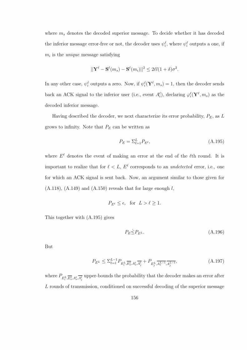
where ms denotes the decoded superior message. To decide whether it has decoded
the inferior message error-free or not, the decoder uses ψℓi , where ψℓ
i outputs a one, if
mi is the unique message satisfying
||Yℓ − Sℓ(ms) − Sℓ(mi)||2 ≤ 2ℓl(1 + δ)σ2.
In any other case, ψℓi outputs a zero. Now, if ψℓ
i (Yℓ, ms) = 1, then the decoder sends
back an ACK signal to the inferior user (i.e., event Aℓi), declaring ϕℓ
i(Yℓ, ms) as the
decoded inferior message.
Having described the decoder, we next characterize its error probability, PE , as L
grows to infinity. Note that PE can be written as
PE = ΣLℓ=1PEℓ, (A.195)
where Eℓ denotes the event of making an error at the end of the ℓth round. It is
important to realize that for ℓ < L, Eℓ corresponds to an undetected error, i.e., one
for which an ACK signal is sent back. Now, an argument similar to those given for
(A.118), (A.149) and (A.150) reveals that for large enough l,
PEℓ ≤ ǫ, for L > ℓ ≥ 1.
This together with (A.195) gives
PE≤PEL. (A.196)
But
PEL ≤ ΣL−1ℓ=1 PEL
i ,Eℓs,Aℓ
s,Aℓj+ P
ELj ,AL−1
s ,AL−1j
, (A.197)
where PEL
i ,Eℓs,Aℓ
s,Aℓjupper-bounds the probability that the decoder makes an error after
L rounds of transmission, conditioned on successful decoding of the superior message
156

at the end of the ℓth round. PEL
j ,AL−1s ,AL−1
j
, on the other hand, upper-bounds the
decoder error probability after L rounds, given that it does not decode any of the
messages by the (L− 1)th round. To characterize PEL
i ,Eℓs,Aℓ
s,Aℓj, notice that
PEL
i ,Eℓs,Aℓ
s,Aℓj≤ min{P
ELi ,Eℓ
s,Aℓs, P
Aℓj}, for L > ℓ ≥ 1. (A.198)
Since we are only interested in the case where L grows to infinity, we can assume that
L is even. Now for L2≥ ℓ ≥ 1, we have
PEL
i ,Eℓs,Aℓ
s≤ P
ELi ,E
L/2s ,A
L/2s
. (A.199)
This is because in the event ELi E
ℓsA
ℓs, ℓ corresponds to the number of rounds during
which the superior user is acting as a DDF relay for the inferior one. Likewise, for
ℓ ≥ L2
+ 1
PAℓ
j≤ P
AL/2j
. (A.200)
This is because in the event Aℓj, ℓ corresponds to the number of rounds during which
the two users are simultaneously transmitting their messages. Clearly, increasing ℓ
reduces PAℓ
j(notice that for exactly the same reason, PEL
j≤ P
EL/2j
). Following the
same steps leading to (A.131) reveals that
PA
L/2j
≤PE
L/2j, (A.201)
which simply states that the probability of sending back a NACK signal is of the same
exponential order as the probability of making a joint error. Now from equations
(A.197) to (A.201), we conclude
PEL≤L
2(P
ELi ,E
L/2s ,A
L/2s
+ PE
L/2j
), for L even. (A.202)
157
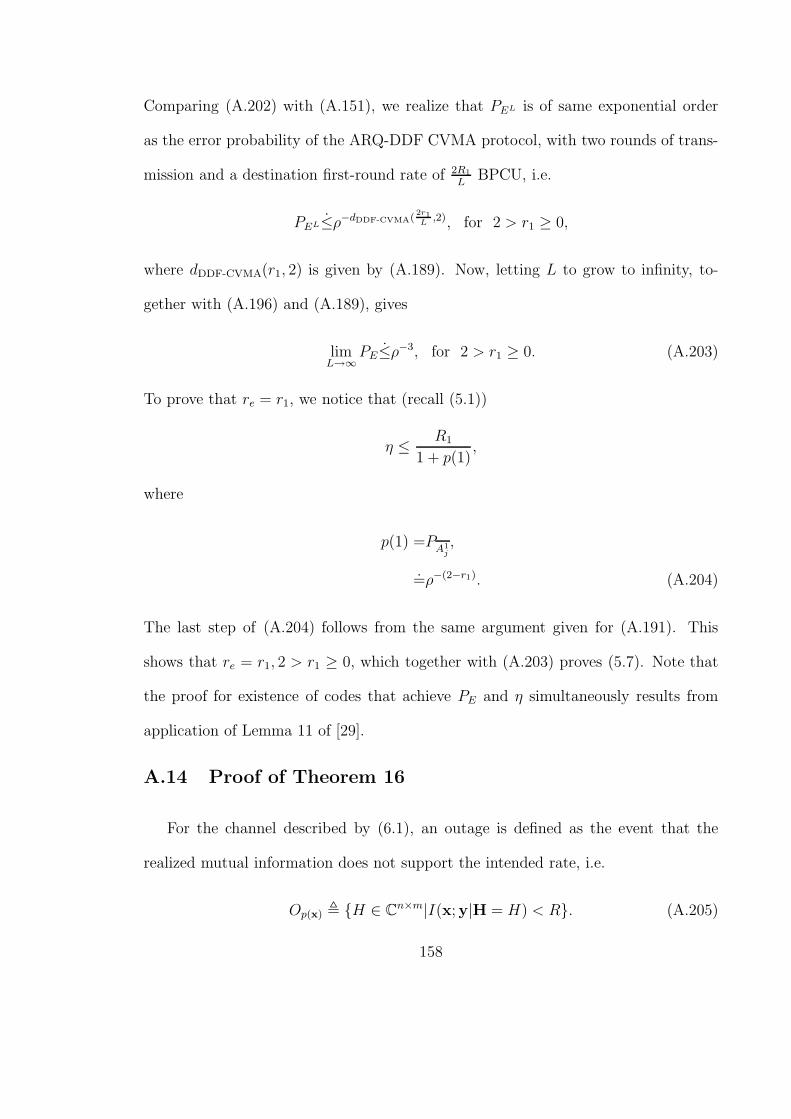
Comparing (A.202) with (A.151), we realize that PEL is of same exponential order
as the error probability of the ARQ-DDF CVMA protocol, with two rounds of trans-
mission and a destination first-round rate of 2R1
LBPCU, i.e.
PEL≤ρ−dDDF-CVMA(2r1L
,2), for 2 > r1 ≥ 0,
where dDDF-CVMA(r1, 2) is given by (A.189). Now, letting L to grow to infinity, to-
gether with (A.196) and (A.189), gives
limL→∞
PE≤ρ−3, for 2 > r1 ≥ 0. (A.203)
To prove that re = r1, we notice that (recall (5.1))
η ≤R1
1 + p(1),
where
p(1) =PA1
j,
=ρ−(2−r1). (A.204)
The last step of (A.204) follows from the same argument given for (A.191). This
shows that re = r1, 2 > r1 ≥ 0, which together with (A.203) proves (5.7). Note that
the proof for existence of codes that achieve PE and η simultaneously results from
application of Lemma 11 of [29].
A.14 Proof of Theorem 16
For the channel described by (6.1), an outage is defined as the event that the
realized mutual information does not support the intended rate, i.e.
Op(x) , {H ∈ Cn×m|I(x;y|H = H) < R}. (A.205)
158
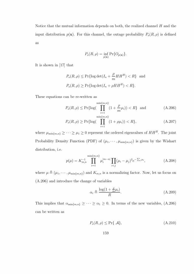
Notice that the mutual information depends on both, the realized channel H and the
input distribution p(x). For this channel, the outage probability Po(R, ρ) is defined
as
Po(R, ρ) = infp(x)
Pr{Op(x)}.
It is shown in [17] that
Po(R, ρ) ≤ Pr{log det(In +ρ
mHHH) < R} and
Po(R, ρ) ≥ Pr{log det(In + ρHHH) < R}.
These equations can be re-written as
Po(R, ρ) ≤ Pr{log(
min{m,n}∏
i=1
(1 +ρ
mµi)) < R} and (A.206)
Po(R, ρ) ≥ Pr{log(
min{m,n}∏
i=1
(1 + ρµi)) < R}, (A.207)
where µmin{m,n} ≥ · · · ≥ µ1 ≥ 0 represent the ordered eigenvalues of HHH. The joint
Probability Density Function (PDF) of (µ1, · · · , µmin{m,n}) is given by the Wishart
distribution, i.e.
p(µ) = K−1m,n
min{m,n}∏
i=1
µ|m−n|i
∏
i<j
(µi − µj)2e−
P
i µi , (A.208)
where µ , (µ1, · · · , µmin{m,n}) and Km,n is a normalizing factor. Now, let us focus on
(A.206) and introduce the change of variables
αi ,log(1 + ρ
mµi)
R. (A.209)
This implies that αmin{m,n} ≥ · · · ≥ α1 ≥ 0. In terms of the new variables, (A.206)
can be written as
Po(R, ρ) ≤ Pr{ A}, (A.210)
159
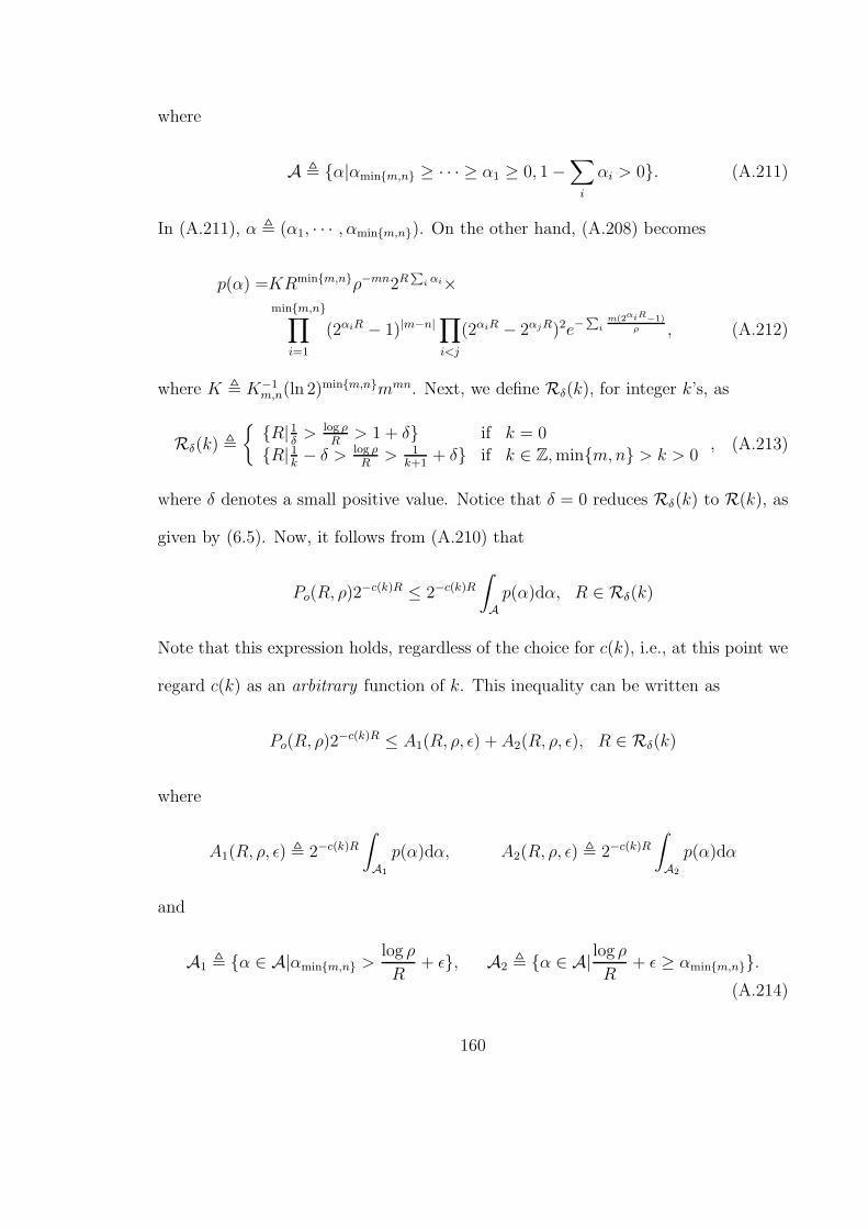
where
A , {α|αmin{m,n} ≥ · · · ≥ α1 ≥ 0, 1 −∑
i
αi > 0}. (A.211)
In (A.211), α , (α1, · · · , αmin{m,n}). On the other hand, (A.208) becomes
p(α) =KRmin{m,n}ρ−mn2RP
i αi×
min{m,n}∏
i=1
(2αiR − 1)|m−n|∏
i<j
(2αiR − 2αjR)2e−P
im(2αiR−1)
ρ , (A.212)
where K , K−1m,n(ln 2)min{m,n}mmn. Next, we define Rδ(k), for integer k’s, as
Rδ(k) ,
{{R|1
δ> log ρ
R> 1 + δ} if k = 0
{R| 1k− δ > log ρ
R> 1
k+1+ δ} if k ∈ Z,min{m,n} > k > 0
, (A.213)
where δ denotes a small positive value. Notice that δ = 0 reduces Rδ(k) to R(k), as
given by (6.5). Now, it follows from (A.210) that
Po(R, ρ)2−c(k)R ≤ 2−c(k)R
∫
A
p(α)dα, R ∈ Rδ(k)
Note that this expression holds, regardless of the choice for c(k), i.e., at this point we
regard c(k) as an arbitrary function of k. This inequality can be written as
Po(R, ρ)2−c(k)R ≤ A1(R, ρ, ǫ) + A2(R, ρ, ǫ), R ∈ Rδ(k)
where
A1(R, ρ, ǫ) , 2−c(k)R
∫
A1
p(α)dα, A2(R, ρ, ǫ) , 2−c(k)R
∫
A2
p(α)dα
and
A1 , {α ∈ A|αmin{m,n} >log ρ
R+ ǫ}, A2 , {α ∈ A|
log ρ
R+ ǫ ≥ αmin{m,n}}.
(A.214)
160
This means that
lim supρ→ ∞
R ∈ Rδ(k)
logPo(R, ρ) − c(k)R
log ρ≤ lim sup
ρ→ ∞R ∈ Rδ(k)
log(1 + A1(R, ρ, ǫ)/A2(R, ρ, ǫ)
)
log ρ+
lim supρ→ ∞
R ∈ Rδ(k)
logA2(R, ρ, ǫ)
log ρ, (A.215)
To characterize the first term in the right-hand side of (A.215), we notice that
A1(R, ρ, ǫ) ≤KRmin{m,n}e
mρ ρ−mn2−c(k)R×
∫
A1
2RP
i αi
min{m,n}∏
i=1
2αi|m−n|R∏
i<j
22αjRe−m2(αmin{m,n}−
log ρR
)R
dα
≤KRmin{m,n}emρ ρ−mn2−c(k)R
∫
A1
2f(α)Re−m2ǫR
dα,
where
f(α) ,
min{m,n}∑
i=1
(|m− n| + 2i− 1)αi. (A.216)
Realizing that Vol{A1} ≤ 1, we conclude
A1(R, ρ, ǫ) ≤KRmin{m,n}(2ǫR)
f1−c(k)ǫ e−m2ǫR
emρ ρ−mn, (A.217)
where
f1 , supA1
f(α).
161
On the other hand
A2(R, ρ, ǫ) ≥KRmin{m,n}e
m min{m,n}ρ ρ−mn2−c(k)R
∫
A2
e−P
i m2−(log ρ
R−αi)R
2RP
i αi×
min{m,n}∏
i=1
(1 − 2−αiR)|m−n|2|m−n|αiR∏
i<j
(1 − 2−(αj−αi)R)222αjRdα,
≥KRmin{m,n}em min{m,n}
ρ ρ−mn2−c(k)R
∫
Aǫ1
e−m min{m,n}2−ǫ1R
2RP
i αi×
min{m,n}∏
i=1
(1 − 2−ǫ1R)|m−n|2|m−n|αiR∏
i<j
(1 − 2−ǫ1R)222αjRdα, (A.218)
where
Aǫ1 , {α ∈ A2|log ρ
R− αmin{m,n} > ǫ1, α1 > ǫ1, |αj − αi| > ǫ1 ∀i 6= j}.
Realizing that e−2−ǫ1R≥ (1 − 2−ǫ1R), (A.218) yields
A2(R, ρ, ǫ) ≥ KRmin{m,n}em min{m,n}
ρ (1 − 2−ǫ1R)m(n+min{m,n})ρ−mn2−c(k)R
∫
Aǫ1
2f(α)Rdα,
where, as before, f(.) is given by (A.216). Let us define α∗ as
α∗ , arg supα∈Aǫ1
f(α).
Then it follows from the continuity of f(.) that, for any ǫ2 > 0, there exists a neigh-
borhood Iǫ2 of α∗, within which
f(α) ≥ f(α∗) − ǫ2.
This means that
A2(R, ρ, ǫ) ≥KRmin{m,n}e
m min{m,n}ρ (1 − 2−ǫ1R)m(n+min{m,n})ρ−mn2−c(k)R
∫
Aǫ1∩Iǫ2
2f(α)Rdα,
A2(R, ρ, ǫ) ≥KRmin{m,n}e
m min{m,n}ρ (1 − 2−ǫ1R)m(n+min{m,n})ρ−mn2(f(α∗)−c(k)−ǫ2)R×
Vol{Aǫ1 ∩ Iǫ2}. (A.219)
162
Now, from (A.217), (A.219) and the fact that e−m(min{m,n}−1)
ρ ≤ 1, we conclude that
A1(R, ρ, ǫ)
A2(R, ρ, ǫ)≤(1 − (2ǫR)−
ǫ1ǫ
)−m(n+min{m,n})(2ǫR)
f1−f(α∗)+ǫ2ǫ e−m(2ǫR)Vol−1{Aǫ1 ∩ Iǫ2}.
(A.220)
This means that
lim supρ→ ∞
R ∈ Rδ(k)
log(1 + A1(R, ρ, ǫ)/A2(R, ρ, ǫ)
)
log ρ= 0 (A.221)
Note that (A.221) holds, whether ρ growing to infinity and R ∈ Rδ(k) result in R
growing to infinity or not. This is because the right hand side of (A.220) decays
exponentially with 2ǫR, while it only grows polynomially with the same variable. To
characterize the second term on the right-hand side of (A.215), we note that
A2(R, ρ, ǫ) ≤KRmin{m,n}ρ−mn2−c(k)R
∫
A2
2RP
i αi
min{m,n}∏
i=1
2αi|m−n|R∏
i<j
22αjRdα,
≤KRmin{m,n}2(f2−c(k))Rρ−mn.
This means that
logA2(R, ρ, ǫ)
log ρ≤
log(KRmin{m,n})
log ρ+ (f2 − c(k))
R
log ρ−mn, (A.222)
where
f2 , supA2
f(α).
To derive f2, one needs to consider two different cases. The first case is when R ∈
Rδ(0), in which case
f2 = m+ n− 1, R ∈ Rδ(0). (A.223)
163

In this case, the supremum is achieved at α∗ = (0, · · · , 0, 1). The second case is when
R ∈ Rδ(k), for k ∈ Z and min{m,n} > k > 0, where
f2 = [m+ n− (2k + 1)] + k(k + 1)(log ρ
R+ ǫ), R ∈ Rδ(k),min{m,n} > k > 0.
(A.224)
The supremum happens at
α∗ = (0, · · · , 1 − k(log ρ
R+ ǫ),
log ρ
R+ ǫ, · · · ,
log ρ
R+ ǫ
︸ ︷︷ ︸
k times
).
Notice that, assuming ǫ ≤ δ, (A.213) guarantees that 1 − k( log ρR
+ ǫ) > 0. Plugging
in for f2 in (A.222), we conclude
logA2(R, ρ, ǫ)
log ρ≤
log(KRmin{m,n})
log ρ− g(k) + (mn− g(k))
R
log ρǫ+
(c(k) − c(k))R
log ρ, for R ∈ Rδ(k). (A.225)
In this expression, g(k) is given by (6.7) and c(k) is defined as
c(k) , m+ n− (2k + 1). (A.226)
Now, from (A.215), (A.221) and (A.225), together with the fact that ǫ can be made
arbitrarily small, one concludes
lim supρ→ ∞
R ∈ Rδ(k)
logPo(R, ρ) − c(k)R
log ρ≤ −g(k)+
(c(k) − c(k)) × lim supρ→ ∞
R ∈ Rδ(k)
R
log ρ. (A.227)
Next we turn our attention to (A.207) and introduce the following change of variables.
βi ,log(1 + ρµi)
R. (A.228)
164
This implies that βmin{m,n} ≥ · · · ≥ β1 ≥ 0. In terms of the new variables, (A.207)
can be written as
Po(R, ρ) ≥ Pr{B}, (A.229)
where
B , {β|βmin{m,n} ≥ · · · ≥ β1 ≥ 0, 1 −∑
i
βi > 0}. (A.230)
In (A.230), β , (β1, · · · , βmin{m,n}). On the other hand, (A.208) becomes
p(β) =KRmin{m,n}ρ−mn2RP
i βi×
min{m,n}∏
i=1
(2βiR − 1)|m−n|∏
i<j
(2βiR − 2βjR)2e−P
i2βiR−1
ρ , (A.231)
where K , K−1m,n(ln 2)min{m,n}. This means that
Po(R, ρ)2−c(k)R ≥ 2−c(k)R
∫
B
p(β)dβ, R ∈ Rδ(k).
Thus
Po(R, ρ)2−c(k)R ≥KRmin{m,n}e
min{m,n}ρ ρ−mn2−c(k)R
∫
B
e−P
i 2−(log ρ
R−βi)R
2RP
i βi×
min{m,n}∏
i=1
(1 − 2−βiR)|m−n|2|m−n|βiR∏
i<j
(1 − 2−(βj−βi)R)222βjRdβ,
≥KRmin{m,n}emin{m,n}
ρ ρ−mn2−c(k)R
∫
Bǫ1
e−min{m,n}2−ǫ1R
2RP
i βi×
min{m,n}∏
i=1
(1 − 2−ǫ1R)|m−n|2|m−n|βiR∏
i<j
(1 − 2−ǫ1R)222βjRdβ, (A.232)
where
Bǫ1 , {β ∈ B|log ρ
R− ǫ1 > βmin{m,n}, β1 > ǫ1, |βj − βi| > ǫ1 ∀i 6= j}.
165

Realizing that e−2−ǫ1R≥ (1 − 2−ǫ1R), (A.232) yields
Po(R, ρ)2−c(k)R ≥ KRmin{m,n}e
min{m,n}ρ (1 − 2−ǫ1R)mn+min{m,n}ρ−mn2−c(k)R
∫
Bǫ1
2f(β)Rdβ,
where, as before, f(.) is given by (A.216). Let us define β∗ as
β∗ , arg supβ∈Bǫ1
f(β).
Again, it follows from the continuity of f(.) that, for any ǫ2 > 0, there exists a
neighborhood Iǫ2 of β∗, within which
f(β) ≥ f(β∗) − ǫ2.
This means that
Po(R, ρ)2−c(k) ≥KRmin{m,n}e
min{m,n}ρ (1 − 2−ǫ1R)mn+min{m,n}ρ−mn2−c(k)R
∫
Bǫ1∩Iǫ2
2f(β)Rdβ,
Po(R, ρ)2−c(k) ≥KRmin{m,n}e
min{m,n}ρ (1 − 2−ǫ1R)mn+min{m,n}ρ−mn2(f(β∗)−c(k)−ǫ2)R×
Vol{Bǫ1 ∩ Iǫ2}.
Thus
lim infρ→ ∞
R ∈ Rδ(k)
logPo(R, ρ) − c(k)R
log ρ≥ −mn+
lim infρ→ ∞
R ∈ Rδ(k)
(f(β∗) − c(k) − ǫ2)R
log ρ. (A.233)
Since (A.233) is valid for arbitrarily small values of ǫ1 and ǫ2, we conclude
lim infρ→ ∞
R ∈ Rδ(k)
logPo(R, ρ) − c(k)R
log ρ≥ −g(k)+
(c(k) − c(k)) × lim infρ→ ∞
R ∈ Rδ(k)
R
log ρ, (A.234)
166

where we have used the fact that B0 = A2|ǫ=0, which means that f(β∗) can be easily
derived from (A.223) and (A.224) by simply plugging in ǫ = 0. Examining (A.227)
and (A.234) reveals that the choice
c(k) = c(k), ∀k (A.235)
guarantees the existence of
limρ→ ∞
R ∈ Rδ(k)
logPo(R, ρ) − c(k)R
log ρ= −g(k), (A.236)
regardless of whether limρ→∞R
log ρexits or not. Now, since (A.236) holds for arbitrarily
small values of δ, we get (6.4). Note that (A.235), together with (A.226), result in
(6.6) and thus complete the proof.
A.15 Proof of Theorem 17
The proof follows that of Theorem 2 in [17]. In particular, we prove (6.17) in two
steps. The first step is to show that
lim infρ→ ∞R ∈ R(k)
logPe(R, ρ) − c(k)R
log ρ≥ −g(k). (A.237)
Towards this end, let us denote the ML error probability, conditioned on a certain
channel realization H , by PE|H. It then follows that
Pe(R, ρ) = EH{PE|H(R, ρ)},
=
∫
PE|H(R, ρ)p(H)dH.
Thus
Pe(R, ρ) ≥
∫
C
PE|H(R, ρ)p(H)dH, (A.238)
167

where C denotes any subset of the set of all channel realizations. Let us define Cǫ as
the set of channel realizations for which the conditional ML error probability cannot
be made smaller than ǫ, i.e.
Cǫ , {H|PE|H(R, ρ) ≥ ǫ}. (A.239)
From (A.238) and (A.239) one concludes that
Pe(R, ρ) ≥ ǫPCǫ(R, ρ),
where
PCǫ(R, ρ) = Pr{Cǫ}. (A.240)
This means that
logPe(R, ρ) − c(k)R
log ρ≥
logPCǫ(R, ρ) − c(k)R
log ρ+
log ǫ
log ρ,
where c(k) is given by (6.6), or
lim infρ→ ∞
R ∈ Rδ(k)
logPe(R, ρ) − c(k)R
log ρ≥ lim inf
ρ→ ∞R ∈ Rδ(k)
logPCǫ(R, ρ) − c(k)R
log ρ, (A.241)
where Rδ(k) is given by (A.213). Now, application of Fano’s inequality reveals that
PE|H(R, ρ) ≥ 1 −I(x;y|H = H)
R−
1
Rl,
where l denotes the codeword length [17]. This, together with (A.239), means that
{H|1 −I(x;y|H = H)
R−
1
Rl≥ ǫ} ⊆ Cǫ,
which using (A.205) results in
PCǫ(R, ρ) ≥ Po((1 − ǫ−1
Rl)R, ρ) or
lim infρ→ ∞
R ∈ Rδ(k)
logPCǫ(R, ρ) − c(k)R
log ρ≥ lim inf
ρ→ ∞R ∈ Rδ(k)
logPo((1 − ǫ)R, ρ) − c(k)R
log ρ.
(A.242)
168
Now, from (A.241) and (A.242), together with the fact that both, δ and ǫ can be
made arbitrarily small, we conclude that
lim infρ→ ∞R ∈ R(k)
logPe(R, ρ) − c(k)R
log ρ≥ lim inf
ρ→ ∞R ∈ R(k)
logPo(R, ρ) − c(k)R
log ρ.
But, from Theorem 16 (refer to (6.4)), we know that the right-hand side equals −g(k)
(given by (6.7)). This proves (A.237) and thus completes the first step.
The second step in proving (6.17) is to show that
lim supρ→ ∞R ∈ R(k)
logPe(R, ρ) − c(k)R
log ρ≤ −g(k), (A.243)
provided that the codeword length, l, satisfies l ≥ m+ n− 1. To prove this, consider
a Gaussian code-book with 2Rl codewords of length l. It is straightforward to verify
that the ML error probability, conditioned on a certain channel realization, is upper-
bounded by
PE|H(R, ρ) ≤ 2Rl det(In +ρ
2mHHH)−l,
= 2Rl
min{m,n}∏
i=1
(1 +ρ
2mµi)
−l, (A.244)
where µmin{m,n} ≥ · · · ≥ µ1 ≥ 0 represent the ordered eigenvalues of HHH. The joint
PDF of (µ1, · · · , µmin{m,n}) is given by (A.208). The change of variables
γi ,log(1 + ρ
2mµi)
R,
changes (A.244) and (A.208), into
PE|γ(R, ρ) ≤ 2(1−Pmin{m,n}
i=1 γi)Rl (A.245)
169
and
p(γ) =KRmin{m,n}ρ−mn2RP
i γi×
min{m,n}∏
i=1
(2γiR − 1)|m−n|∏
i<j
(2γiR − 2γjR)2e−P
i2m(2γiR−1)
ρ ,
where γ , (γ1, · · · , γmin{m,n}) and K , K−1m,n(ln 2)min{m,n}(2m)mn. Next we define D
as
D , {γ|γmin{m,n} ≥ · · · ≥ γi ≥ 0, 1 −
min{m,n}∑
i=1
γi ≥ 0}.
Referring to (A.245) reveals that D consists of those channel realizations for which
the upper-bound on the ML error probability cannot be made arbitrarily small, even
through the use of infinitely long codewords. For these channel realizations, we upper-
bound PE|γ(R, ρ) by 1, i.e.
Pe(R, ρ) = PE,Dc(R, ρ) + PE,D(R, ρ),
Pe(R, ρ) ≤ PE,Dc(R, ρ) + PD(R, ρ), (A.246)
where Dc denotes the complement of D. Let us first focus on PD(R, ρ). Realizing
that D is precisely the same set as A (refer to (A.211)) and that, up to a scaling
factor, p(γ) is identical to p(α) (refer to (A.212)), it follows immediately that
lim supρ→ ∞R ∈ R(k)
logPD(R, ρ) − c(k)R
log ρ≤ −g(k). (A.247)
Now, turning our attention back to PE,Dc(R, ρ), we realize that
limρ→ ∞R ∈ R(k)
PE,Dc1(R, ρ)2−c(k)R = 0, (A.248)
170
which means that
lim supρ→ ∞R ∈ R(k)
logPE,Dc(R, ρ) − c(k)R
log ρ= lim sup
ρ→ ∞R ∈ R(k)
logPE,Dc2(R, ρ) − c(k)R
log ρ,
(A.249)
where
Dc1 , {γ /∈ D|γmin{m,n} >
log ρ
R} and Dc
2 , {γ /∈ D|γmin{m,n} ≤log ρ
R}.
Notice that (A.248) holds for exactly the same reason as (A.221) does (refer to the
comment after (A.221)). Now, using (A.245), we have
PE,Dc2(R, ρ)2−c(k)R = 2−c(k)R
∫
Dc2
PE|γ(R, ρ)p(γ)dγ,
≤ KRmin{m,n}ρ−mn2−c(k)R
∫
Dc2
2[f(γ)+l(1−Pmin{m,n}
i=1 γi)]Rdγ,
where
f(γ) , 2P
i(|m−n|+2i−1)γiR.
Thus
PE,Dc2(R, ρ)2−c(k)R ≤ KRmin{m,n}ρ−mn2(f2−c(k))RVol{Dc
2}, (A.250)
where
f2 , supDc
2
f(γ) + l(1 −
min{m,n}∑
i=1
γi).
Realizing that for l ≥ m+n−1, the supremum occurs at γ = γ∗, such that 1−∑γ∗i =
0, f2 can be easily derived from (A.223) and (A.224) by simply plugging in ǫ = 0.
Therefore, (A.250) gives
lim supρ→ ∞R ∈ R(k)
logPE,Dc2(R, ρ) − c(k)R
log ρ≤ −g(k). (A.251)
171
Now, from (A.251), (A.249) and (A.247), we conclude (A.243), which together with
(A.237), proves (6.17). Since we proved (6.17) using an ensemble of Gaussian codes,
it follows that, for any code-length l ≥ m + n − 1, there exists at least a code, for
which (6.17) holds. This completes the proof.
A.16 Proof of Theorem 18
Realizing that the V-BLAST protocol essentially transforms the m × m MIMO
channel into a multiple-access channel with m single-antenna users and a destination
with m receive antennas, we prove (6.18) by following the same lines as that of
Theorem 2 in [18]. In particular, let ES denote the event that a certain decoder
makes errors in decoding the codewords transmitted by a subset S of the antennas.
It then follows that
∑
S 6=∅
Pr{ES} ≥ Pe(R, ρ). (A.252)
It is also clear that
Pe(R, ρ) ≥ Pr{ES∗}, (A.253)
where S∗ denotes any non-empty subset of {1, · · · , m}. Let us define S∗ as the non-
empty subset of {1, · · · , m}, such that for all other non-empty subsets S, we have
lim infρ→ ∞
|S|mR ∈ RS(k)
|S∗|mR ∈ RS∗(k∗)
(
gS(k) − gS∗(k∗))
−( |S|
mcS(k) −
|S∗|
mcS∗(k∗)
) R
log ρ≥ 0. (A.254)
In (A.254), |S| denotes the cardinality of set S. Also, RS(k), cS(k) and gS(k) denote
R(k), c(k) and g(k), as defined by (6.5), (6.6) and (6.7), for a MIMO channel with
172

|S| transmit and m receive antennas. The proof of (6.18) then follows in three steps.
First, we prove that for any decoder
lim infρ→ ∞
|S∗|mR ∈ RS∗(k∗)
Pe(R, ρ) −|S∗|mcS∗(k)R
log ρ≥ −gS∗(k∗). (A.255)
This follows immediately from (A.253) and the fact that Pr{ES∗} upper-bounds the
ML error probability of a MIMO channel with |S∗| transmit antennas, m receive
antennas and rate |S∗|mR. The second step in proving (6.18) is to show that there
exists a code, along with a decoder, for which
lim supρ→ ∞
|S∗|mR ∈ RS∗(k∗)
Pe(R, ρ) −|S∗|mcS∗(k∗)R
log ρ≤ −gS∗(k∗). (A.256)
We prove this by showing that the error probability of the joint ML decoder, averaged
over the ensemble of Gaussian codes, satisfies (A.256). The existence of the desired
code then follows from the fact that there exist codes in the ensemble that perform
at least as well as the average. For this purpose, assume that each of the antennas
uses a Gaussian code-book of code-word length l = 2m + 1 and size 2Rm
l codewords.
It then follows from Theorem 17, (refer to (6.17)), that
limρ→ ∞
|S|mR ∈ RS(k)
log Pr{ES} −|S|mcS(k)R
log ρ= −gS(k), ∀S 6= ∅, (A.257)
which means
limρ→ ∞
|S|mR ∈ RS(k)
|S∗|mR ∈ RS∗(k∗)
[
log Pr{ES}/Pr{ES∗}
log ρ+(
gS(k) − gS∗(k∗))
−
( |S|
mcS(k) −
|S∗|
mcS∗(k∗)
) R
log ρ
]
= 0. (A.258)
173

Now, (A.258), together with (A.254), results in
lim supρ→ ∞
|S|mR ∈ RS(k)
|S∗|mR ∈ RS∗(k∗)
log Pr{ES}/Pr{ES∗}
log ρ≤ 0, ∀S 6= ∅. (A.259)
Returning to (A.252), we have
log(1 +∑
S 6=S∗,∅Pr{ES}Pr{ES∗}
)
log ρ+
log Pr{ES∗} − |S∗|mcS∗(k∗)R
log ρ≥
logPe(R, ρ) −|S∗|mcS∗(k∗)R
log ρ.
Taking the lim sup of both sides, together with (A.259) and (A.257) results in (A.256).
Notice that (A.255) and (A.256) mean that
limρ→ ∞
|S∗|mR ∈ RS∗(k∗)
Pe(R, ρ) −|S∗|mcS∗(k)R
log ρ= −gS∗(k∗). (A.260)
The third and last step in proving (6.18) is to show that |S∗| = 1. One can prove this
directly using the definitions of R(k), c(k) and g(k) (equations (6.5), (6.6) and (6.7)).
However, we choose to do this using observations (6.8) and (6.9). In particular, notice
that based on these observations, (A.254) reduces to finding the subset S∗, for which
dS(|S|
mr) − dS∗(
|S∗|
mr) ≥ 0, ∀S 6= ∅,
where dS(r) represents the DMT for a MIMO system with |S| transmit and m receive
antennas. From the proof of Theorem 3 in [18], we know that |S∗| = 1. Now, this
together with (A.260) results in (6.18) and thus completes the proof.
174
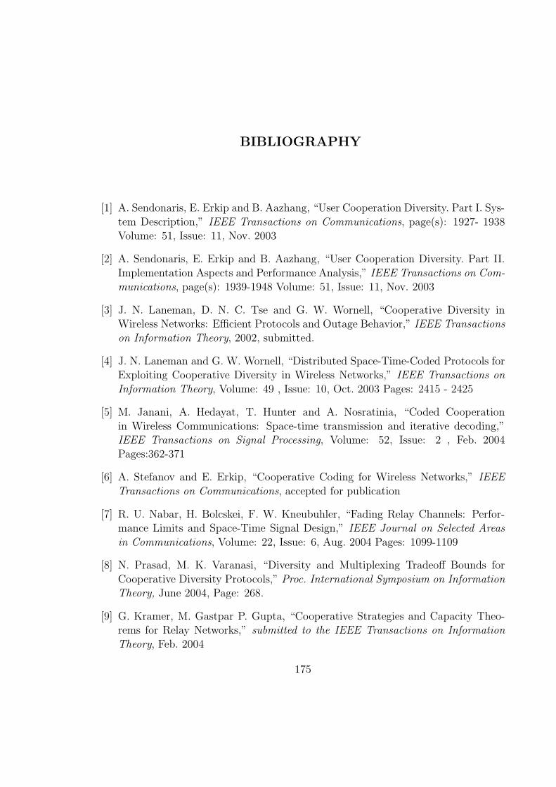
BIBLIOGRAPHY
[1] A. Sendonaris, E. Erkip and B. Aazhang, “User Cooperation Diversity. Part I. Sys-
tem Description,” IEEE Transactions on Communications, page(s): 1927- 1938
Volume: 51, Issue: 11, Nov. 2003
[2] A. Sendonaris, E. Erkip and B. Aazhang, “User Cooperation Diversity. Part II.
Implementation Aspects and Performance Analysis,” IEEE Transactions on Com-munications, page(s): 1939-1948 Volume: 51, Issue: 11, Nov. 2003
[3] J. N. Laneman, D. N. C. Tse and G. W. Wornell, “Cooperative Diversity inWireless Networks: Efficient Protocols and Outage Behavior,” IEEE Transactions
on Information Theory, 2002, submitted.
[4] J. N. Laneman and G. W. Wornell, “Distributed Space-Time-Coded Protocols forExploiting Cooperative Diversity in Wireless Networks,” IEEE Transactions on
Information Theory, Volume: 49 , Issue: 10, Oct. 2003 Pages: 2415 - 2425
[5] M. Janani, A. Hedayat, T. Hunter and A. Nosratinia, “Coded Cooperation
in Wireless Communications: Space-time transmission and iterative decoding,”IEEE Transactions on Signal Processing, Volume: 52, Issue: 2 , Feb. 2004
Pages:362-371
[6] A. Stefanov and E. Erkip, “Cooperative Coding for Wireless Networks,” IEEE
Transactions on Communications, accepted for publication
[7] R. U. Nabar, H. Bolcskei, F. W. Kneubuhler, “Fading Relay Channels: Perfor-mance Limits and Space-Time Signal Design,” IEEE Journal on Selected Areas
in Communications, Volume: 22, Issue: 6, Aug. 2004 Pages: 1099-1109
[8] N. Prasad, M. K. Varanasi, “Diversity and Multiplexing Tradeoff Bounds for
Cooperative Diversity Protocols,” Proc. International Symposium on InformationTheory, June 2004, Page: 268.
[9] G. Kramer, M. Gastpar P. Gupta, “Cooperative Strategies and Capacity Theo-rems for Relay Networks,” submitted to the IEEE Transactions on Information
Theory, Feb. 2004
175
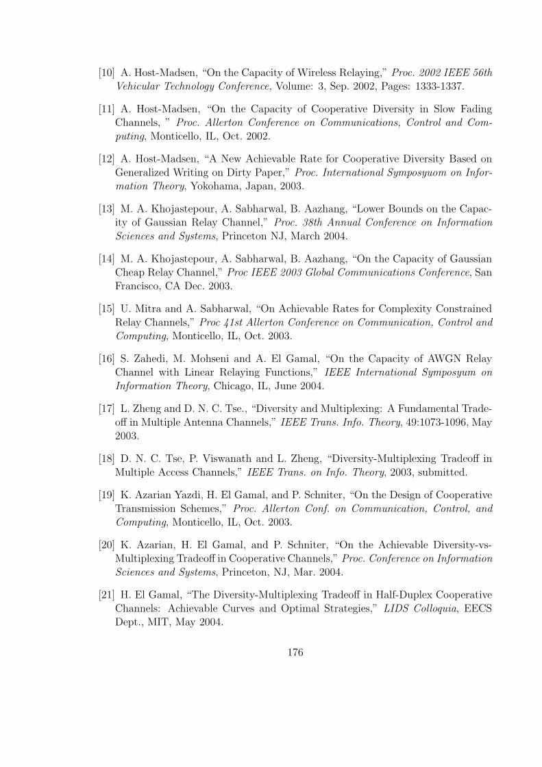
[10] A. Host-Madsen, “On the Capacity of Wireless Relaying,” Proc. 2002 IEEE 56thVehicular Technology Conference, Volume: 3, Sep. 2002, Pages: 1333-1337.
[11] A. Host-Madsen, “On the Capacity of Cooperative Diversity in Slow FadingChannels, ” Proc. Allerton Conference on Communications, Control and Com-
puting, Monticello, IL, Oct. 2002.
[12] A. Host-Madsen, “A New Achievable Rate for Cooperative Diversity Based on
Generalized Writing on Dirty Paper,” Proc. International Symposyuom on Infor-mation Theory, Yokohama, Japan, 2003.
[13] M. A. Khojastepour, A. Sabharwal, B. Aazhang, “Lower Bounds on the Capac-ity of Gaussian Relay Channel,” Proc. 38th Annual Conference on Information
Sciences and Systems, Princeton NJ, March 2004.
[14] M. A. Khojastepour, A. Sabharwal, B. Aazhang, “On the Capacity of GaussianCheap Relay Channel,” Proc IEEE 2003 Global Communications Conference, San
Francisco, CA Dec. 2003.
[15] U. Mitra and A. Sabharwal, “On Achievable Rates for Complexity Constrained
Relay Channels,” Proc 41st Allerton Conference on Communication, Control andComputing, Monticello, IL, Oct. 2003.
[16] S. Zahedi, M. Mohseni and A. El Gamal, “On the Capacity of AWGN RelayChannel with Linear Relaying Functions,” IEEE International Symposyum on
Information Theory, Chicago, IL, June 2004.
[17] L. Zheng and D. N. C. Tse., “Diversity and Multiplexing: A Fundamental Trade-
off in Multiple Antenna Channels,” IEEE Trans. Info. Theory, 49:1073-1096, May
2003.
[18] D. N. C. Tse, P. Viswanath and L. Zheng, “Diversity-Multiplexing Tradeoff in
Multiple Access Channels,” IEEE Trans. on Info. Theory, 2003, submitted.
[19] K. Azarian Yazdi, H. El Gamal, and P. Schniter, “On the Design of Cooperative
Transmission Schemes,” Proc. Allerton Conf. on Communication, Control, andComputing, Monticello, IL, Oct. 2003.
[20] K. Azarian, H. El Gamal, and P. Schniter, “On the Achievable Diversity-vs-Multiplexing Tradeoff in Cooperative Channels,” Proc. Conference on Information
Sciences and Systems, Princeton, NJ, Mar. 2004.
[21] H. El Gamal, “The Diversity-Multiplexing Tradeoff in Half-Duplex Cooperative
Channels: Achievable Curves and Optimal Strategies,” LIDS Colloquia, EECSDept., MIT, May 2004.
176
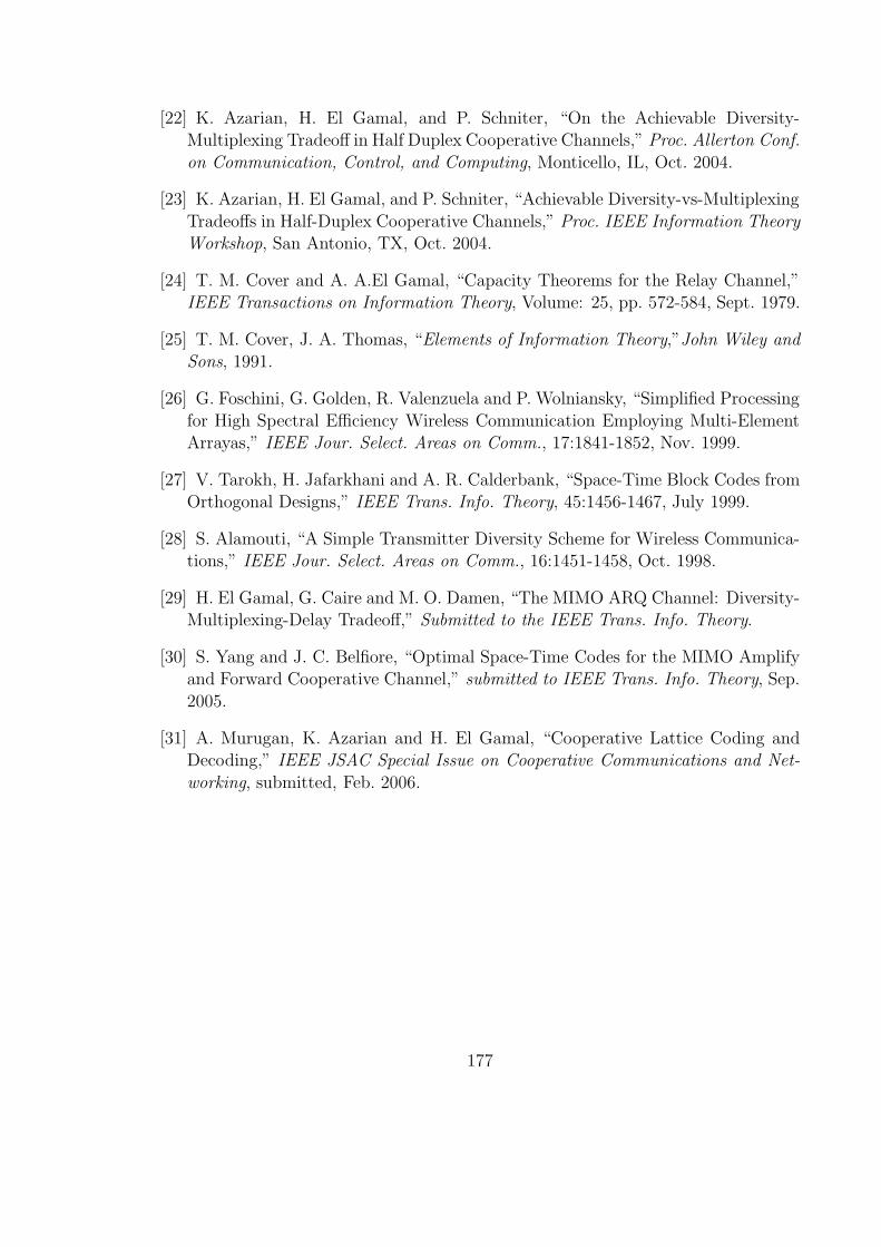
[22] K. Azarian, H. El Gamal, and P. Schniter, “On the Achievable Diversity-Multiplexing Tradeoff in Half Duplex Cooperative Channels,” Proc. Allerton Conf.
on Communication, Control, and Computing, Monticello, IL, Oct. 2004.
[23] K. Azarian, H. El Gamal, and P. Schniter, “Achievable Diversity-vs-Multiplexing
Tradeoffs in Half-Duplex Cooperative Channels,” Proc. IEEE Information TheoryWorkshop, San Antonio, TX, Oct. 2004.
[24] T. M. Cover and A. A.El Gamal, “Capacity Theorems for the Relay Channel,”IEEE Transactions on Information Theory, Volume: 25, pp. 572-584, Sept. 1979.
[25] T. M. Cover, J. A. Thomas, “Elements of Information Theory,”John Wiley andSons, 1991.
[26] G. Foschini, G. Golden, R. Valenzuela and P. Wolniansky, “Simplified Processing
for High Spectral Efficiency Wireless Communication Employing Multi-ElementArrayas,” IEEE Jour. Select. Areas on Comm., 17:1841-1852, Nov. 1999.
[27] V. Tarokh, H. Jafarkhani and A. R. Calderbank, “Space-Time Block Codes fromOrthogonal Designs,” IEEE Trans. Info. Theory, 45:1456-1467, July 1999.
[28] S. Alamouti, “A Simple Transmitter Diversity Scheme for Wireless Communica-tions,” IEEE Jour. Select. Areas on Comm., 16:1451-1458, Oct. 1998.
[29] H. El Gamal, G. Caire and M. O. Damen, “The MIMO ARQ Channel: Diversity-Multiplexing-Delay Tradeoff,” Submitted to the IEEE Trans. Info. Theory.
[30] S. Yang and J. C. Belfiore, “Optimal Space-Time Codes for the MIMO Amplifyand Forward Cooperative Channel,” submitted to IEEE Trans. Info. Theory, Sep.
2005.
[31] A. Murugan, K. Azarian and H. El Gamal, “Cooperative Lattice Coding andDecoding,” IEEE JSAC Special Issue on Cooperative Communications and Net-
working, submitted, Feb. 2006.
177