Outage Analysis in MIMOFree-Space Optical Channels

with Pulse-Position Modulation

N. Letzepis and A. Guillen i Fabregas

CUED / F-INFENG / TR 597February 2008

1

Outage Analysis in MIMO Free-Space OpticalChannels with Pulse-Position Modulation

Nick Letzepis and Albert Guillen i Fabregas

Abstract

Free space optical communication is an attractive alternative to radio frequency for the purpose of transmittingdata on the order of gigabits per second. The main drawback in communicating via the free space opticalchannel is the detrimental effect the atmosphere has on a propagating laser beam. Atmospheric turbulence causesrandom fluctuations in the irradiance of the received optical laser beam, commonly referred to as scintillation. Thescintillation process is slow compared to the large data rates typical of optical transmission. As such, we adopt aquasi-static block fading model and study the outage probability of the channel under the assumption of orthogonalpulse-position modulation. We investigate the mitigation of scintillation through the use of multiple lasers andmultiple apertures, thereby creating a multiple-input multiple output (MIMO) channel. Non-ideal photodetection isalso assumed such that the combined shot noise and thermal noise are considered as signal-independent additiveGaussian white noise. Assuming perfect receiver channel state information (CSI), we compute the signal-to-noiseratio exponents for the cases when the scintillation is lognormal, exponential, gamma-gamma and lognormal-Ricedistributed, which cover a wide range of atmospheric turbulence conditions. Furthermore, we illustrate very largegains, in some cases larger than 20 dB, when transmitter CSI is also available by adapting the transmitted electricalpower.

N. Letzepis is with Institute for Telecommunications Research, University of South Australia, SPRI Building - Mawson Lakes Blvd.,Mawson Lakes SA 5095, Australia, e-mail: nick.letzepis@unisa.edu.au.

A. Guillen i Fabregas is with the Department of Engineering, University of Cambridge, Cambridge CB2 1PZ, UK, e-mail:guillen@ieee.org.

2

I. INTRODUCTION

Free space optical (FSO) communication offers an attractive alternative to the radio frequency (RF)channel for the purpose of transmitting data at very high rates. By utilising a high carrier frequency in theoptical range, digital communication on the order of gigabits per second is possible. In addition, FSO linksare difficult to intercept, immune to interference or jamming from external sources, and are not subject tofrequency spectrum regulations. FSO communications have received recent attention in applications suchas satellite communications, fiber-backup, RF-wireless back-haul and last-mile connectivity [1].

The main drawback of the FSO channel is the detrimental effect the atmosphere has on a propa-gating laser beam. The atmosphere is composed of gas molecules, water vapor, pollutants, dust, andother chemical particulates that are trapped by Earth’s gravitational field. Since the wavelength of atypical optical carrier is comparable to these molecule and particle sizes, the carrier wave is subject tovarious propagation effects that are uncommon to RF systems. One such effect is scintillation, caused byatmospheric turbulence, and refers to random fluctuations in the irradiance of the received optical laserbeam (analogous to fading in RF systems) [2–4].

Recent works on the mitigation of scintillation concentrate on the use of multiple-lasers and multiple-apertures to create a multiple-input-multiple-output (MIMO) channel [5–13]. Many of these works considerscintillation as an ergodic fading process, and analyse the channel in terms of its ergodic capacity. However,compared to typical data rates, scintillation is a slow time-varying process (with a coherence time on theorder of milliseconds), and it is therefore more appropriate to analyse the outage probability of the channel.To some extent, this has been done in the works of [6, 10, 12–14]. In [6, 13] the outage probability of theMIMO FSO channel is analysed under the assumption of ideal photodetection (PD) (i.e. PD is modeledas a Poisson counting process) with no bandwidth constraints. Wilson et al. [10] also assume perfectPD, but with the further constraint of pulse-position modulation (PPM). Lee and Chan [12], study theoutage probability under the assumption of on-off keying (OOK) transmission and non-ideal PD, i.e. thecombined shot noise and thermal noise process is modeled as zero mean signal independent additive whiteGaussian noise (AWGN). Farid and Hranilovic [14] extend this analysis to include the effects of pointingerrors.

In this report we study the outage probability of the MIMO FSO channel under the assumptions ofPPM, non-ideal PD, and equal gain combining (EGC) at the receiver. In particular, we model the channelas a quasi-static block fading channel whereby communication takes place over a finite number of blocksand each block of transmitted symbols experiences an independent identically distributed (i.i.d.) fadingrealisation [15, 16]. Given the slow time-varying nature of scintillation, channel state information (CSI)can be estimated at the receiver and fed back to the transmitter via a dedicated feedback link. We considertwo types of CSI knowledge. First we assume perfect CSI is available only at the receiver (CSIR case),and the transmitter knows only the channel statistics. We study a number of scintillation distributions, i.e.,lognormal, modelling weak turbulence; exponential, modelling strong turbulence; gamma-gamma [17] andlognormal-Rice [18, 19], modelling a wide range of turbulence conditions. For the CSIR-only case, wederive signal-to-noise ratio (SNR) exponents and show that these exponents are composed of a channelrelated parameter (dependent on the scintillation distribution) times the Singleton bound [20–22]. Thenwe consider the case when perfect CSI is known at both the transmitter and receiver (CSIT case). For thiscase, the transmitter finds the optimal power allocation to minimise the outage probability [23]. Usingresults from [24], we derive the optimal power allocation that minimises the outage probability, subject toshort- and long-term power constraints. We show that under a long-term power constraint, very large powersavings can be achieved, and that the delay-limited capacity [25] always exists for lognormal distributedscintillation, whereas, for the exponential, gamma-gamma and lognormal-Rice cases, one must code overseveral blocks for delay-limited capacity to exist. The number of required blocks depends on the rate ofthe binary code via the SNR exponent. We show that with the use of MIMO one needs only to code overa single realisation to ensure the existance of delay-limited capacity. These results highlight the benefitsof MIMO and block diversity in reducing the outage probability in FSO systems.

3

The report is organised as follows. In Section II, we define the channel model and assumptions.In Section III we review the lognormal, exponential, gamma-gamma and lognormal-Rice scintillationmodels. Section IV defines the outage probability and presents results on the minimum-mean squared error(MMSE). Then in Sections V and VI we present the main results of our asymptotic outage probabilityanalysis for the CSIR and CSIT cases, respectively. Concluding remarks are then given in Section VII.Proofs of the various results can be found in the Appendices.

II. SYSTEM MODEL

We consider an FSO system with M transmit lasers an N aperture receiver as shown in Figure 1.Information data is first encoded by a binary code of rate Rc. The encoded stream is modulated accordingto a Q-ary PPM scheme, resulting in rate R = Rc log2 Q (bits/channel use). Repetition transmission isemployed such that the same PPM signal is transmitted in perfect synchronism by each of the M lasersthrough an atmospheric turbulent channel and collected by N receive apertures. We assume the distancebetween the individual lasers and apertures is sufficient so that spatial correlation is negligible. At eachaperture, the received optical signal is converted to an electrical signal via PD. Non-ideal PD is assumedsuch that the combined shot noise and thermal noise processes can be modeled as zero mean, signalindependent AWGN (an assumption commonly used in the literature, see e.g. [3–5, 12, 14, 26–31]).

Encoder

PPM

PPM

Laser

Laser

Atmospheric Turbulence

Aperture PD

PD

Decoder

Aperture

1

M N

1

......

Transmitter Receiver

Fig. 1. Block diagram of an FSO MIMO system.

In FSO communications, channel variations are typically much slower than the signaling period. Assuch, we model the channel as a non-ergodic block-fading channel, for which a given codeword of lengthBL undergoes only a finite number B of scintillation realisations [15, 16]. The received signal at aperture1 ≤ n ≤ N can be written as

ynb [`] =

(M∑

m=1

hm,nb

)√pb xb[`] + zn

b [`], (1)

for b = 1, . . . , B, ` = 1, . . . , L, where ynb [`], zn

b [`] ∈ RQ are the received and noise signals at block b,time instant ` and aperture n, xb[`],∈ RQ is the transmitted signal at block b and time instant `, andhm,n

b denotes the scintillation fading coefficient between laser m and aperture n. Each transmitted symbolis drawn from a PPM alphabet, xb[`] ∈ X ppm ∆

= {e1, . . . , eQ}, where eq is the canonical basis vector,

4

i.e., it has all zeros except for a one in position q, the time slot where the pulse is transmitted. Thenoise samples of zn

b [`] are independent realisations of a random variable Z ∼ N (0, 1), and pb denotes thereceived electrical power of block b at each aperture in the absence of scintillation. The fading coefficientshm,n

b are independent realisations of a random variable H with probability density function (pdf) fH(h).At the receiver, we assume equal gain combining (EGC) is employed, such that

yb[`] =1√N

N∑n=1

ynb [`] (2)

=1√N

N∑n=1

M∑m=1

hm,nb

√pbxb[`] +

1√N

N∑n=1

znb [`] (3)

= M√

Npb hb xb[`] + zb[`], (4)

where

hb =1

MN

M∑m=1

N∑n=1

hm,nb (5)

and

zb[`] =1√N

N∑n=1

znb [`] ∼ N (0, 1). (6)

Letting hb∆= hb/

√E[h2

b ] givesyb[`] =

√pbhbxb[`] + zb[`], (7)

wherepb = M2NE[h2

b ]pb. (8)

Hence (7) can be considered as a SISO channel with an equivalent fading coefficient hb, normalized suchthat E[H2] = 1.1Thus, the average received electrical SNR can be expressed as snr , E[ph2

b ] = E[pb].We will consider two cases of channel state information (CSI). We will first study the case of perfect

CSIR, and we will then consider the case of perfect CSIT as well as CSIR. In the case where we haveonly CSIR, we will distribute the electrical power uniformly over the blocks, i.e., pb = p = snr forb = 1, . . . , B. Otherwise, in the case of CSIT, we will allocate electrical power in order to improveperformance. In particular, in the case of perfect CSIR and CSIT, we will consider the following twoelectrical power constraints

Short-term:1

B

B∑b=1

pb ≤ P (9)

Long-term: E

[1

B

B∑b=1

pb

]≤ P. (10)

Throughout the report, we will devote special attention to the case of B = 1, i.e., the channel does notvary within a codeword. This scenario is relevant for FSO, since, due to the large data-rates, one is ableto transmit millions of bits virtually over the same channel realisation. We will see that most results admitvery simple forms, and some times, even closed form. This analysis allows for a system characterisationwhere the expressions highlight the roles of the key design parameters.

1For ideal PD, the normalisation E[H] = 1 is used to keep optical power constant. We assume non-ideal PD and work entirely in theelectrical domain. Hence, we chose the normalisation E[H2] = 1, used commonly in RF fading channels. Since we consider only theasymptotic behaviour of the outage probability, the specific normalisation is irrelevant and does not affect our results.

5

III. SCINTILLATION DISTRIBUTIONS

The scintillation pdf, fH(h), is parameterised by the scintillation index (SI),

σ2I ,

Var(H)

(E[H])2. (11)

Under weak atmospheric turbulence conditions (defined as those regimes for which σ2I < 1), the SI is

proportional to the so called Rytov variance which represents the SI of an unbounded plane wave in weakturbulence conditions, and is also considered as a measure of the strength of the optical turbulence understrong-fluctuation regimes [4]. As the Rytov variance increases, the SI continues to increase beyond theweak turbulence regime until it reaches a maximum value greater than unity. At that point the SI beginsto decrease with increasing Rytov variance and approaches unity from above. This region is termed thesaturation region [17, 32].

The distribution of the irradiance fluctuations is dependent on the strength of the optical turbulence.For the weak turbulence regime, the fluctuations are generally considered to be lognormally distributed,and for very strong turbulence, exponentially distributed [2, 33]. For moderate turbulence, the distributionof the fluctuations is not well understood, and a number of distributions have been proposed, such asthe lognormal-Rice distribution [4, 17, 19, 34, 35] (also known as the Beckmann distribution [36]) and K-distribution [34]. In [17], Al-Habash et al. proposed a gamma-gamma distribution as a general model forall levels of atmospheric turbulence. Moreover, recent work in [35] has shown that the gamma-gammamodel is in close agreement with experimental measurements under moderate-to-strong turbulence condi-tions. In this report we focus on lognormal, exponential, gamma-gamma and lognormal-Rice distributedscintillation.

For MIMO-EGC FSO communication systems, hb and hb are realisations of random variables H andH respectively, which are functions of hm,n

b for m = 1, . . . ,M and n = 1, . . . , N . In (8) we can determineE[H2] in terms of the scintillation index,

E[H2] =E[H2]

MN+

(MN − 1)

MNE[H]2 = E[H]2

(1 +

σ2I

MN

)(12)

Hence the mean and variance of H is therefore

E[H] =E[H]√E[H2]

=1√

1 +σ2

I

MN

. (13)

var[H] = E[H2]− E[H]2 = 1− 1

1 +σ2

I

MN

. (14)

A. Lognormal ScintillationFor lognormal distributed scintillation,

fH(h) =1

hσ√

2πexp

(−(log h− µ)2/(2σ2)

), (15)

where µ and σ are related to the SI via µ = − log(1 + σ2I ) and σ2 = log(1 + σ2

I ). The distribution of Hresults from a summation of MN lognormal distributions, for which the pdf is unknown. However, it iswell known that the distribution resulting from the sum of independent lognormal random variables canbe accurately approximated by a lognormal distribution [37–40], i.e.

fH(h) ≈ 1

hσ√

2πexp

(−(log h− µ)2/(2σ2)

), (16)

6

where from (13) and (14) we have

µ = − log

(1 +

σ2I

MN

)(17)

σ2 = log

(1 +

σ2I

MN

). (18)

Thus as M, N →∞, µ, σ2 → 0 and the distribution becomes more concentrated about a mean of 1, i.e.the system approaches the non-fading channel.

The distribution of H can also be computed numerically by performing an (MN − 1)-fold convolutionor via a fast Fourier transform (FFT) method. The later approach, being less computationally expensive,involves performing the FFT of a truncated lognormal distribution, raising it to the MN th power and thencomputing the inverse-FFT (IFFT) (details are given in Appendix I). The accuracy of the FFT methoddepends both on the truncation and the length of the FFT. Fig. 2 compares the PDF of H computednumerically using the FFT method (with hmax = 64 and NFFT = 221) to the log-normal approximation.It can be seen that the lognormal approximation is quite a good fit except for the right hand side tail, forwhich the approximation tends to over-estimate.

10−2

10−1

100

101

102

10−10

10−8

10−6

10−4

10−2

100

h

fH

(h)

histogramPDFPDF approx.

MN = 1

MN = 4

MN = 64

Fig. 2. PDF of H when H is a lognormal random variable with σ2I = 1 : solid line shows simulation results; dashed line shows PDF

computed numerically via FFT method and the dot-dashed line shows the lognormal approximation (16).

B. Exponential ScintillationFor exponential distributed scintillation,

fH(h) = λ exp(−λh). (19)

7

Note that this corresponds to the super-saturated turbulence regime, for which σ2I = 1. We may also

interpret H as a Gamma distributed random variable, since fH(h) = g(h; 1, 1/λ) where [41, Ch. 17]

g(h; k, θ) = hk−1 exp(−h/θ)

θkΓ(k). (20)

Since sums of Gamma distributed random variables are also Gamma distributed [41, Ch. 17] we have,

fH(h) = g

(h; MN ;

1

λMN

)(21)

andE[H2] =

1

λ2

(1 +

1

MN

). (22)

The normalized combined fading coefficient is

fH(h) = g(h; MN ; (MN(1 + MN))−

12

), (23)

which is independent of λ. Fig. 3 plots (23) for MN = 1, 4, 64.

10−2

10−1

100

101

102

10−10

10−8

10−6

10−4

10−2

100

h

fH

(h)

MN = 1MN = 4MN = 64

Fig. 3. PDF of H when H is exponential distributed (23).

C. Gamma-Gamma ScintillationThe gamma-gamma distribution arises from the product of two independent Gamma distributed random

variables and [17],

fH(h) =2(αβ)

α+β2

Γ(α)Γ(β)h

α+β2−1 Kα−β(2

√αβh), (24)

8

where Kν(x) denotes the modified Bessel function of the second kind. The parameters α and β are relatedwith the scintillation index via σ2

I = α−1 + β−1 + (αβ)−1.The moments of h can be determined via

E[Hk] =Γ(α + k)Γ(β + k)

Γ(α)Γ(β)(αβ)−k , (25)

or recursively usingE[Hk] = E[Hk−1](k − 1 + α)(k − 1 + β)(αβ)−1. (26)

Hence, E[H] = 1 and E[H2] = 1/(1 + σ2I ).

Unfortunately, finding a closed form expression for the distribution resulting from sums of Gamma-Gamma distributed random variables is difficult. We can however obtain the moment generating function(MGF) from which we can obtain the distribution of H via the inverse Fourier transform. First considerthe following theorem..

Theorem 3.1: The moment generating function (MGF) of the Gamma-Gamma distribution (24) is givenby

MH(t) = 2 F0(α, β; t/(αβ)), (27)

for t < 0, where 2 F0 denotes the generalized hypergeometric function.Proof: See Appendix II-A.

Note that the hypergeometric function (27) may also be written as [42, Ch. 13]

2 F0(α, β; t/(αβ)) =

(−αβ

t

)α

U

(α, 1 + α− β,−αβ

t

),

where U(a, b, z) = 1Γ(a)

∫∞0

e−zt(t−1)a−1tb−a−1 dt. Furthermore, for the special case, β = 1 correspondingto K-distributed scintillation [4, Sec. 9.9.1], we have

2 F0(α, 1; t/α) = exp(−α

t

)(−α

t

)α

Γ(1− α,−α

t

),

where Γ(a, x)∆=∫∞

xta−1 exp(−t)dt denotes the upper incomplete gamma function [42, p.260].

Setting t = jω in (27), one obtains the characteristic function. The characteristic function of a sum ofindependent random variables is equal to the multiplication of their respective characteristic functions [43].Hence, by taking the inverse Fourier transform, the pdf of H and H are respectively

fH(h) =MN

2π

∫ ∞

−∞[2 F0(α, β; jω/(αβ))]MN exp (−jωMNh) dω, (28)

fH(h) =

[1 +

σ2I

MN

] 12

fH

([1 +

σ2I

MN

] 12

h

). (29)

In addition to (29) we may also compute the PDF of H using the FFT method (as in the casefor lognormal H). The FFT method turns out to be much faster than performing the integration (29)numerically. Fig. 4 compares the PDF of H using the FFT method (dashed line) to histograms of 108

i.i.d. samples from H (solid).From [4, 17] the gamma-gamma cdf is given by:

FH(h) =(αβh)αΓ(β − α)

αΓ(α)Γ(β)1 F2(α; 1 + α, 1 + α− β; αβh)

+(αβh)βΓ(α− β)

βΓ(α)Γ(β)1 F2(β; 1 + β, 1 + β − α; αβh) (30)

Note (30) is not valid when α = β, or when |α−β| is an integer. However, for small h, we can circumventthis problem by using the following approximation.

9

10−2

10−1

100

101

102

10−10

10−8

10−6

10−4

10−2

100

h

fH

(h)

histogramPDF

MN = 1

MN = 4

MN = 64

Fig. 4. PDF of H when H is Gamma-Gamma distributed with α = 2.05 and β = 2.45: solid lines, histogram of randomly generatedsamples; dashed lines, numerical computation using the FFT method.

Proposition 3.1: For small h the cdf of a gamma-gamma distributed random variable can be approxi-mated as

FH(h) ≈

{α2(α−1)

(Γ(α))2

[1 + 2α log 1

2α+ α log 1

h

]hα, β = α

Γ(|α−β|)Γ(α)Γ(β)

(αβh)min(α,β)

min(α,β), β 6= α

(31)

Proof: See Appendix II-B.Fig. 5 illustrates the convergence of (31) to (30) as h decreases. This figure shows that the approximationis tight as h → 0.

D. Lognormal-Rice ScintillationFor the lognormal-Rice distribution, like the gamma-gamma case, the fading random variable is written

as the product of two independent random variables, H = XY , where X is a lognormal distributedrandom variable with parameters σ2 and µ = −σ2/2, and

√Y Rice distributed random variable, i.e.

f√Y (y) =y

σ2R

exp

(−y2 + ν2

R

2σ2R

)I0

(yνR

σ2R

,

)(32)

where I0(z) denotes the modified Bessel function of the first kind, and the parameters of the distributionare set to

σ2R =

1

2(r + 1), νR =

√r

r + 1. (33)

Hence the pdf of Y is

fY (y) = (r + 1) exp(−r − (r + 1)y)I0

(√4r(r + 1)y

)(34)

10

10−4 10−3 10−2 10−1 10010−10

10−8

10−6

10−4

10−2

100

h

FH

(h)

CDFapprox.

Fig. 5. Gamma-gamma cdf (30) (solid) and the approximation (31) (dashed) for α = 2.05 and β = 2.45.

The parameter r is referred to as the coherence parameter [34], and is also well known as the Ricefactor in the analysis of RF fading channels with a line of sight component. When r = 0, (32) becomesa Rayleigh pdf and the system reduces to the lognormal-exponential case. As r →∞ the pdf approachesa unit impulse function at y = 1. In other words as r → ∞, Y → 1, and the scintillation is purelylognormal distributed (weak turbulence case). Furthermore, as r, σ → 0, the lognormal-Rice distributionreduces to the exponential distribution. Therefore, the lognormal-Rice distribution includes the lognormal,lognormal-exponential and exponential distributions as special cases.

The overall distribution of H = XY has no closed form expression, but can be written in integralform [4]

fH(h) =(1 + r)e−r

√2πσ

∫ ∞

0

1

z2I0

(2

√(1 + r)rh

z

)exp

(−(1 + r)h

z− 1

2σ2

(log z +

1

2σ2

)2)

dz (35)

It is easy to show that for the scintillation distribution given by (35), the SI is given by

σ2I = exp(σ2)

(1 +

1 + 2r

(r + 1)2

)− 1. (36)

Despite its complicated pdf, as will be shown later, we will still be able to determine the correspondingasymptotic outage probability behaviour in the general MIMO case.

IV. OUTAGE PROBABILITY, MUTUAL INFORMATION AND MMSEThe channel described by (7) under the quasi-static assumption is not information stable [44] and

therefore, the channel capacity in the strict Shannon sense is zero. It can be shown that the codeword

11

error probability of any coding scheme can be lower bounded by the information outage probability [15,16],

Pout(snr, R) = Pr(I(p, h) < R), (37)

where R is the transmission rate and I(p, h) is the instantaneous input-output mutual information fora given power allocation p , (p1, . . . , pB), and vector channel realisation h , (h1, . . . , hB). Theinstantaneous mutual information can be expressed as [45]

I(p, h) =1

B

B∑b=1

Iawgn(pbh2b), (38)

where Iawgn(ρ) is the input-output mutual information of an AWGN channel with SNR ρ. For PPM [26]

Iawgn(ρ) = log2 Q− E

[log2

(1 + exp(−ρ)

Q∑q=2

exp (√

ρ(Zq − Z1))

)], (39)

where Zq ∼ N (0, 1) for q = 1, . . . , Q. We can show the following result.Proposition 4.1: The input-output mutual information for Q-PPM transmission over an AWGN channel

with SNR ρ can be lower bounded by

Iawgn(ρ) ≥ Iawgnlb (ρ)

∆= log2 Q− EU

[log2

(1 + (Q− 1) exp

(−ρ

2−√ρU

))](40)

where U ∼ N (0, 1).Proof: See Appendix III.

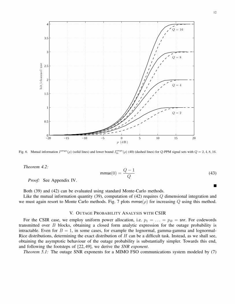
Since U ∼ N (0, 1), the lower bound (40) can be efficiently computed using Gauss-Hermite quadra-tures [42]. Note that (40) was derived by [46] using the law of large numbers, and the authors consideredit as an approximation. Here we proved that it is not just an approximation, but also a bound to themutual information. Furthermore, as Q increases, Iawgn(ρ) → Iawgn

lb (ρ), i.e., Iawgnlb (ρ) is asymptotically

tight for large Q. This can be observed in Fig 6, where the mutual information and the lower bound (40)are plotted for various values of Q. Remark that the bound (40) will lead to an upper bound to the outageprobability.

For the CSIT case we will use the recently discovered relationship between mutual information andthe MMSE [47]. This relationship states that2

d

dρIawgn(ρ) =

mmse(ρ)

log(2)(41)

where mmse(ρ) is the MMSE in estimating the input from the output of a Gaussian channel as a functionof the SNR ρ. For the case of PPM, we can express the MMSE as follows.

Theorem 4.1: Suppose QPPM symbols are transmitted across an AWGN channel with SNR ρ. Then,the MMSE is

mmse(ρ) = 1− E

exp(2√

ρ(√

ρ + Z1)) + (Q− 1) exp(2√

ρZ2)(exp(ρ) exp(

√ρZ1) +

∑Qk=2 exp(

√ρZk)

)2

, (42)

where Zi ∼ N (0, 1) for i = 1, . . . , Q.Proof: See Appendix IV.

A more careful look at the MMSE, yields the following result, which is relevant in the wideband regime[48].

2The log(2) term arises because we have defined Iawgn(ρ) in bits/channel usage.

12

−20 −15 −10 −5 0 5 10 15 200

0.5

1

1.5

2

2.5

3

3.5

4

ρ (dB )

bit

/ch

an

nel

use

Q = 16

Q = 8

Q = 4

Q = 2

Fig. 6. Mutual information Iawgn(ρ) (solid lines) and lower bound Iawgnlb (ρ) (40) (dashed lines) for Q-PPM signal sets with Q = 2, 4, 8, 16.

Theorem 4.2:mmse(0) =

Q− 1

Q(43)

Proof: See Appendix IV.

Both (39) and (42) can be evaluated using standard Monte-Carlo methods.Like the mutual information quantity (39), computation of (42) requires Q dimensional integration and

we must again resort to Monte Carlo methods. Fig. 7 plots mmse(ρ) for increasing Q using this method.

V. OUTAGE PROBABILITY ANALYSIS WITH CSIRFor the CSIR case, we employ uniform power allocation, i.e. p1 = . . . = pB = snr. For codewords

transmitted over B blocks, obtaining a closed form analytic expression for the outage probability isintractable. Even for B = 1, in some cases, for example the lognormal, gamma-gamma and lognormal-Rice distributions, determining the exact distribution of H can be a difficult task. Instead, as we shall see,obtaining the asymptotic behaviour of the outage probability is substantially simpler. Towards this end,and following the footsteps of [22, 49], we derive the SNR exponent.

Theorem 5.1: The outage SNR exponents for a MIMO FSO communications system modeled by (7)

13

−20 −15 −10 −5 0 5 10 15 200

0.1

0.2

0.3

0.4

0.5

0.6

0.7

0.8

0.9

1

ρ (dB )

mm

se(ρ

)

Fig. 7. Computation of mmse(ρ) (in dB) via Monte Carlo evaluation for Q = 2, 4, 8, 16. Larger Q corresponds to a higher mmse(ρ) curve.

are given as follows:

dln(log snr)2 =

MN

8 log(1 + σ2I )

(1 + bB (1−Rc)c) (44)

dexp(log snr) =

MN

2(1 + bB (1−Rc)c) , (45)

dgg(log snr) =

MN

2min(α, β) (1 + bB (1−Rc)c) , (46)

dlr(log snr) =

MN

2(1 + bB (1−Rc)c) , (47)

for lognormal, exponential, gamma-gamma and lognormal-Rice respectively, where Rc = R/ log2(Q) isthe rate of the binary code and

d(log snr)k∆= − lim

snr→∞

log Pout(snr, R)

(log snr)kk = 1, 2. (48)

Proof: See the Appendix.Proposition 5.1: The outage SNR exponents for a MIMO FSO communications system modeled by (7)

are given in Theorem 5.1, are achievable by random coding over PPM constellations whenever B (1−Rc)is not an integer.

Proof: The proof follows from the proof of Theorem 5.1 and the proof of [22, Th. 1].The above results imply that the outage exponents given by (44)-(47) are the optimal SNR exponents

over the channel: the outage probability is a lower bound to the error probability of any coding scheme, itscorresponding exponents (given in Theorem 5.1) are an upper bound to the exponent of coding schemes.

14

From Proposition 5.1, we can achieve the outage exponents with a particular coding scheme (randomcoding, in this case), and therefore, the exponents given in Theorem 5.1 are optimal.

From (44)-(47) we immediately see the benefits of spatial and block diversity on the system. In particular,each exponent is proportional to: the number of lasers times the number of apertures, reflecting the spatialdiversity; a channel related parameter that is dependent on the scintillation distribution; and the Singletonbound, which is the optimal rate-diversity tradeoff for Rayleigh-faded block fading channels [20–22].

Comparing the channel related parameters in (44)-(47) the effects of the scintillation distribution on theoutage probability are directly visible. For the lognormal case, the channel related parameter is 8 log(1+σ2

I )and hence is directly linked to the SI. Moreover, for small σ2

I < 1, 8 log(1 + σ2I ) ≈ 8σ2

I and the SNRexponent is inversely proportional to the SI. For the exponential case, the channel related parameter isa constant 1/2 as expected, since the SI is constant. For the gamma-gamma case the channel relatedparameter is min(α, β)/2, which highlights an interesting connection between the outage probability andrecent results in the theory of optical scintillation. For gamma-gamma distributed scintillation, the fadingcoefficient results from the product of two independent random variables, i.e. H = XY , where X and Ymodel fluctuations due to large scale and small scale cells. Large scale cells cause refractive effects thatmainly distort the wave front of the propagating beam, and tend to steer the beam in a slightly differentdirection (i.e. beam wander). Small scale cells cause scattering by diffraction and therefore distort theamplitude of the wave through beam spreading and irradiance fluctuations [4, p. 160]. The parameters α, βare related to the large and small scale fluctuation variances via α = σ−2

X and β = σ−2Y . For a plane wave

(neglecting inner/outer scale effects) σ2Y > σ2

X , and as the strength of the optical turbulence increases,the small scale fluctuations dominate and σ2

Y → 1 [4, p. 336]. This implies that the SNR exponent isexclusively dependent on the small scale fluctuations. Moreover, in the strong fluctuation regime, σ2

Y → 1,the gamma-gamma distribution reduces to a K-distribution [4, p. 368], and the system has the same SNRexponent as the exponential case typically used to model very strong fluctuation regimes. In the caseof lognormal-Rice scintillation, we observe that the exponent is exactly equal to that of exponentialscintillation. Remark, however, that this does not imply that the two distributions yield the same outageprobability. The inclusion of the Ricean component results in an error floor whose exponent is the sameas that of the exponential distribution.

In comparing the lognormal exponent with the rest, we observe a striking difference. For the lognormalcase (44) implies the outage probability is dominated by a (log(snr))2 term, whereas for the other cases itis dominated by a log(snr) term. Thus the outage probability decays much more rapidly with SNR for thelognormal case than it does for the exponential or gamma-gamma cases. Furthermore, for the lognormalcase, the slope of the outage probability curve, when plotted on a log-log scale, will not converge to aconstant value. In fact, a constant slope curve will only be observed when plotting the outage probabilityon a log-(log)2 scale.

In deriving (44) (see Appendix V-A) we do not rely on the lognormal approximation, which has beenused in e.g. [5, 12, 31] to simplify the analysis of FSO MIMO links in the presence of lognormal distributedscintillation. Under this approximation, we have an approximate exponent

d(log snr)2 ≈1

8 log(1 +σ2

I

MN)(1 + bB (1−Rc)c) . (49)

Comparing (44) and (49) we see that although the lognormal approximation also exhibits a (log(snr))2

term, it has a different slope than the true SNR exponent. The difference is due to the lognormalapproximation of the sum of random variables and the fact that the left tails of the true distributionand the approximation have different behaviours (see Fig. 2). However, for very small σ2

I , using theapproximation log(1 + x) ≈ x in (44) and (49) we see that they are approximately equal. This behaviouris shown in Fig. 8, which also shows that as σ2

I increases, the lognormal approximation (49) tends tounderestimate the SNR exponent and worsens as MN increases.

15

10−1

100

101

10−2

10−1

100

101

102

σ2I

d (lo

gsnr)2

True exponent.Lognorm approx.

Fig. 8. Comparison of the SNR exponent (44) (solid) to the lognormal approximation (49) (dashed) for B = 1, Q = 2, snrawgn1/2 = 3.18

dB and MN = 1, 2, 4, 8, 16 (highest curve pair corresponds to MN = 16).

For the special case of single block transmission, B = 1, it is straightforward to express the outageprobability in terms of the cumulative distribution function (cdf) of the scintillation random variable, i.e.

Pout(snr, R) = FH

(√snrawgn

R

snr

)(50)

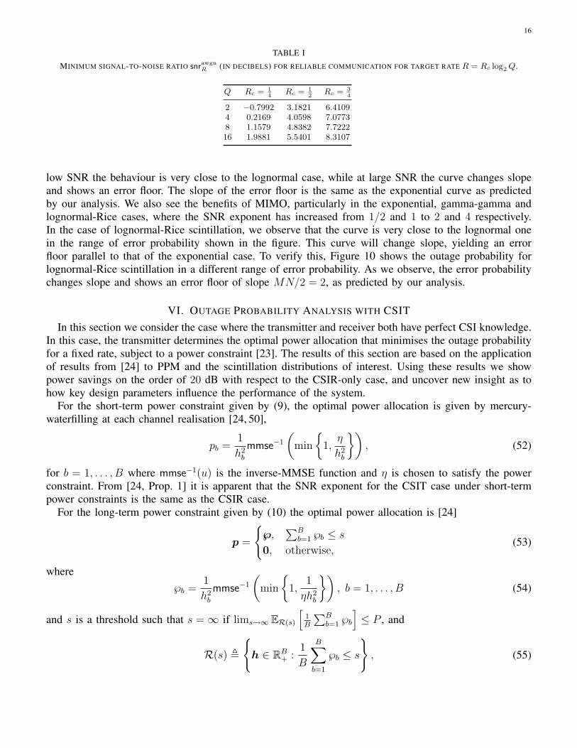
where FH(h) denotes the cdf of H , and snrawgnR

∆= Iawgn,−1(R) denotes the SNR value at which the

mutual information is equal to R. Table I reports these values for Q = 2, 4, 8, 16 and R = Rc log2 Q,with Rc = 1

4, 1

2, 3

4. Therefore, for B = 1, we can compute the outage probability analytically when

the distribution of H is available, i.e., in the exponential case for M, N ≥ 1 or in the lognormal andgamma-gamma cases for M, N = 1. In the case of exponential scintillation we have that

Pout(snr, R) = Γ

(MN,

(MN(1 + MN)

snrawgnR

snr

) 12

), (51)

where Γ(a, x) , 1Γ(a)

∫ x

0ta−1 exp(−t) dt denotes the regularised (lower) incomplete gamma function [42,

p.260]. As mentioned in Section III and described in the Appendix I, it is possible to evaluate thedistribution numerically using the FFT, yielding very accurate computations of the outage probability forB = 1 and M, N ≥ 1 in only a few seconds.

Outage probability curves for the B = 1 case are shown in Fig. 9. For the lognormal case, we seethat the curves do not have constant slope for large SNR, while, for the exponential and gamma-gammacases, a constant slope is clearly visible. In the case of lognormal-Rice scintillation, we observe that for

16

TABLE I

MINIMUM SIGNAL-TO-NOISE RATIO snrawgnR (IN DECIBELS) FOR RELIABLE COMMUNICATION FOR TARGET RATE R = Rc log2 Q.

Q Rc = 14

Rc = 12

Rc = 34

2 −0.7992 3.1821 6.41094 0.2169 4.0598 7.07738 1.1579 4.8382 7.722216 1.9881 5.5401 8.3107

low SNR the behaviour is very close to the lognormal case, while at large SNR the curve changes slopeand shows an error floor. The slope of the error floor is the same as the exponential curve as predictedby our analysis. We also see the benefits of MIMO, particularly in the exponential, gamma-gamma andlognormal-Rice cases, where the SNR exponent has increased from 1/2 and 1 to 2 and 4 respectively.In the case of lognormal-Rice scintillation, we observe that the curve is very close to the lognormal onein the range of error probability shown in the figure. This curve will change slope, yielding an errorfloor parallel to that of the exponential case. To verify this, Figure 10 shows the outage probability forlognormal-Rice scintillation in a different range of error probability. As we observe, the error probabilitychanges slope and shows an error floor of slope MN/2 = 2, as predicted by our analysis.

VI. OUTAGE PROBABILITY ANALYSIS WITH CSITIn this section we consider the case where the transmitter and receiver both have perfect CSI knowledge.

In this case, the transmitter determines the optimal power allocation that minimises the outage probabilityfor a fixed rate, subject to a power constraint [23]. The results of this section are based on the applicationof results from [24] to PPM and the scintillation distributions of interest. Using these results we showpower savings on the order of 20 dB with respect to the CSIR-only case, and uncover new insight as tohow key design parameters influence the performance of the system.

For the short-term power constraint given by (9), the optimal power allocation is given by mercury-waterfilling at each channel realisation [24, 50],

pb =1

h2b

mmse−1

(min

{1,

η

h2b

}), (52)

for b = 1, . . . , B where mmse−1(u) is the inverse-MMSE function and η is chosen to satisfy the powerconstraint. From [24, Prop. 1] it is apparent that the SNR exponent for the CSIT case under short-termpower constraints is the same as the CSIR case.

For the long-term power constraint given by (10) the optimal power allocation is [24]

p =

{℘,

∑Bb=1 ℘b ≤ s

0, otherwise,(53)

where℘b =

1

h2b

mmse−1

(min

{1,

1

ηh2b

}), b = 1, . . . , B (54)

and s is a threshold such that s = ∞ if lims→∞ ER(s)

[1B

∑Bb=1 ℘b

]≤ P , and

R(s) ,

{h ∈ RB

+ :1

B

B∑b=1

℘b ≤ s

}, (55)

17

0 10 20 30 40 50 60 70 8010

−10

10−8

10−6

10−4

10−2

100

snr (dB)

Pout(s

nr,R

)

LNExpGGLN-Rice

MN = 1

MN = 4

Fig. 9. Outage probability for lognormal (solid), exponential distributed (dashed), gamma-gamma distributed scintillation (dot-dashed) andlognormal-Rice (dotted) with σ2

I = 1, α = 2, β = 3 (for gamma-gamma scintillation), σ = 0.7301 and r = 10 (for lognormal-Ricescintillation) B = 1, Q = 2, Rc = 1/2, snrawgn

1/2 = 3.18 dB.

otherwise, s is chosen such that P = ER(s)

[1B

∑Bb=1 ℘b

]. In (54), η is now chosen to satisfy the rate

constraint1

B

B∑b=1

Iawgn

(mmse−1

(min

{1,

1

ηh2b

}))= R (56)

From [24], the long-term SNR exponent is given by

dlt(log snr) =

dst(log snr)

1−dst(log snr)

dst(log snr) < 1

∞ dst(log snr) > 1

, (57)

where dst(log snr) is the short-term SNR exponent, i.e., the SNR exponent obtained in the previous section.

Note that dlt(log snr) = ∞ implies the outage probability curve is vertical, i.e. delay-limited capacity [25]

exists. From (44) we see that dst(log snr) = ∞ for the lognormal case, i.e. delay-limited capacity always

exists, and the outage probability curve is vertical. In the exponential and lognormal-Rice case from (45)and (47) we require that MN (1 + bB (1−Rc)c) > 2, while in the gamma-gamma case from (46) weneed MN min(α, β) (1 + bB (1−Rc)c) > 2, for delay-limited capacity to exist. In other words, for thesecases, M, N, B and Rc need to be chosen carefully to ensure the existance of delay-limited capacity.

18

0 10 20 30 40 50 60 70 80 90 10010−40

10−30

10−20

10−10

100

snr (dB)

1

Pout(s

nr,R

)

1

LN-Rice, MN = 4

1

y = c exp(−2 log snr)

1

Fig. 10. Outage probability for lognormal-Rice with σ2I = 1, σ = 0.7301 and r = 10 B = 1, MN = 4, Q = 2, Rc = 1/2, snrawgn

1/2 = 3.18dB.

Single block transmission (B = 1) is most relevant in FSO communications since the coherence timeis on the order of milliseconds which is large compared to typical data rates. In this case the solution (54)can be determined explicitly since

η =(h2mmse(Iawgn,−1(R))

)−1=(h2mmse(snrawgn

R ))−1

. (58)

Therefore,

℘opt =snrawgn

R

h2. (59)

Intuitively, (59) implies that for single block transmission, whenever snrawgnR /h2 ≤ s, one simply transmits

at the minimum power necessary so that the received instantaneous SNR is equal to the SNR threshold

(snrawgnR ) of the code. Otherwise, transmission is turned off. Thus an outage occurs whenever h <

√snrawgn

R

sand hence

Pout(snr, R) = FH

(√snrawgn

R

γ−1(snr)

)(60)

where γ−1(snr) is the solution to the equation γ(s) = snr, i.e.,

γ(s) = snrawgnR

∫ ∞

ν

fH(h)

h2dh, (61)

19

where ν ,√

snrawgnR

s. In the cases where the distribution of H is known in closed form, Eq. (61) can be

solved explicitly, hence yielding the exact outage probability expression when combined with (60). Forlognormal distributed scintillation and B = M = N = 1, the integral (59) can be solved explicitly,

γln(s) =1

2snrawgn

R (1 + σ2I )

4erfc

(3 log(1 + σ2

I ) + 12log snrawgn − 1

2log s√

2 log(1 + σ2I )

). (62)

We also find thatlims→∞

snrln(s) = snrawgnR (1 + σ2

I )4, (63)

which is precisely the threshold SNR at which Pout(snr, R) → 0. For exponential distributed scintillationwith B = 1 , we obtain,

γexp(s) = snrawgnR

MN(1 + MN)

(MN − 1)(MN − 2)Γ

(MN − 2,

√MN(1 + MN)

snrawgnR

s

). (64)

Similarly, for the case when MN > 2,

lims→∞

snrexp(s) = snrawgnR

MN(1 + MN)

(MN − 1)(MN − 2). (65)

For the case when MN ≤ 2, there exists no threshold SNR for which Pout(snr, R) → 0. This isinteresting, because it means that a combined total of more than 3 lasers and apertures is required todrive Pout(snr, R) → 0 under strong turbulence conditions, unlike the weak turbulence case (lognormal),where a threshold s exists for any MN to drive Pout(snr, R) → 0.

Fig. 11 compares the outage probability for the B = 1 CSIT case (with long-term power constraints)for each of the scintillation distributions. For the MN = 1 case we see that delay-limited capacity onlyexists in the lognormal case, since for the other two distributions dst

(log snr) < 1. In this situation, one mustcode over more blocks to ensure the existance of delay-limited capacity. When MN = 4, delay-limitedcapacity exists in all three distribution cases since dst

(log snr) > 1. Note that the SNR threshold at whichPout → 0 can be determined by computing the expectation snrawgn

R E [H−2], which, as described above,can be determined explicitly for some cases. Comparing the CSIR and CSIT cases (Figs. 9 and 11) wecan see that very large power savings are possible when CSI is known at the transmitter. For example,for the case of gamma-gamma scintillation, at 10−4 we observe around 20 dB gain with power control(for MN = 4).

VII. CONCLUSIONS

In this report we have analysed the outage probability of the MIMO Gaussian FSO channel under theassumption of PPM and non-ideal PD, for lognormal, exponential, gamma-gamma and lognormal-Ricedistributed scintillation. When CSI is known only at the receiver, we have shown that the SNR exponentis proportional to the number lasers and apertures, times a channel related parameter (dependent on thescintillation distribution), times the Singleton bound, even in the cases where a closed form expressionof the equivalent SISO channel distribution is not available in closed-form. When the scintillation islognormal distributed, we have shown that the outage probability is dominated by a (log(snr))2 term,whereas for the exponential, gamma-gamma and lognormal-Rice cases it is dominated by a log(snr) term.When CSI is also known at the transmitter, we applied the power control techniques of [24] to PPM toshow very significant power savings.

20

−5 0 5 10 15 20 25 3010

−10

10−8

10−6

10−4

10−2

100

snr (dB)

Pout(s

nr,R

)

LNExpGGLN-Rice

MN = 4

MN = 1

Fig. 11. Comparison of CSIR and CSIT outage probabilities for lognormal (solid), exponential (dashed), gamma-gamma (dash-dotted) andlognormal-Rice (dotted) distributed scintillation with σ2

I = 1, α = 2, β = 3 (for gamma-gamma scintillation), σ = 0.7301 and r = 10 (forlognormal-Rice scintillation), B = 1, Q = 2, snrawgn

1/2 = 3.18 dB.

APPENDIX IFAST FOURIER TRANSFORM METHOD

This appendix describes how to use the fast Fourier transform (FFT) to numerically compute thedistribution of sums of i.i.d. random variables.

1) Set ∆h = hmax

NFFT, where hmax and NFFT are the truncation value and FFT length respectively.

2) Compute φ[n] = cMNfH(cMN∆hn) for n = 0, . . . , NFFT−1, where c =

√E[H2] is given by (12).

3) Approximate the characteristic function via the discrete Fourier transform (DFT), i.e.

Φ[k] = ∆h

NFFT−1∑n=0

φ[n] exp(−j2πkn/NFFT) (66)

for k = 0 . . . , NFFT − 1, which can be computed efficiently using an FFT algorithm.4) Now compute the distribution by performing the inverse DFT (using an IFFT algorithm) as follows,

fH(∆hn) =1

∆h

1

NFFT

NFFT−1∑k=0

(Φ[k])MN exp(j2πkn/NFFT), (67)

for n = 0 . . . , NFFT − 1.

21

APPENDIX IIGAMMA-GAMMA DISTRIBUTION PROOFS

A. Proof of Theorem 3.1We begin using the property that the Gamma-Gamma distributed random variable can be written as

the product of two independent Gamma distributed random variables X and Y , i.e. pX(x) = g(x; α, 1/α)and pX(y) = g(y; β, 1/β) where g(k, θ) is defined as in (20). Hence we have

Mh(t) = E[exp(tXY )]

=

∫ ∞

0

∫ ∞

0

exp(txy)g(x; α, 1/α)g(y; β, 1/β) dxdy

=

∫ ∞

0

(1− t

αy

)−α

g(y; β, 1/β) dy (68)

=∞∑i

(α + i− 1

i

)(t

α

)i ∫ ∞

0

yig(y; β, 1/β) dy (69)

=∞∑i=0

Γ(α + i)

Γ(α)i!

(t

α

)iΓ(β + i)

Γ(β)βi

=∞∑i=0

(α)i(β)i

i!

(t

αβ

)i

= 2 F0(α, β; t/(αβ)),

where in (68) we used the MGF of a Gamma distributed random variable and in (69) we used the Binomialtheorem.

B. Proof of Proposition 3.1For small h the gamma-gamma pdf can be approximated as

fH(h) ≈

{2α2α

(Γ(α))2hα−1 log 1

2α√

h, β = α

Γ(|α−β|)Γ(α)Γ(β)

(αβh)min(α,β)−1, β 6= α,

where we have used K0(x) ∼ − log(x) and Kν(x) ∼ 12Γ(ν)

(2x

)ν for ν > 0 and x → 0 [42, p. 375]. Theresult therefore follows via simple integration.

22

APPENDIX IIIPROOF OF PROPOSITION 4.1

Using Jensen’s inequality [45] we have that

Iawgn(ρ) = log2 Q− Ey|x=e1

[log2

(1 +

Q∑q=2

exp (√

ρ(yq − y1))

)](70)

≥ log2 Q− Ey1|x=e1

[log2

(1 +

Q∑q=2

Eyq |x=e1 [exp (√

ρ(yq − y1))]

)](71)

= log2 Q− Ey1|x=e1

[log2

(1 + exp(−√ρy1)

Q∑q=2

Eyq |x=e1 [exp (√

ρyq)]

)](72)

= log2 Q− Ey1|x=e1

[log2

(1 + (Q− 1) exp(−√ρy1) exp

(ρ

2

))](73)

= log2 Q− EU

[log2

(1 + (Q− 1) exp(−√ρ(

√ρ + U)) exp

(ρ

2

))](74)

= log2 Q− EU

[log2

(1 + (Q− 1) exp

(−ρ

2−√ρU

))](75)

where (73) follows from yq ∼ N (0, 1) for q = 2, . . . , Q, which implies that exp(√

ρyq) is lognormal withmean exp

(ρ2

).

23

APPENDIX IVPROOF OF THEOREM 4.1

The MMSE estimate is given by

x = E [x|y] (76)

=∑x∈X

xp(x|y) (77)

=∑x∈X

xp(y|x)p(x)

p(y)(78)

=∑x∈X

xp(y|x)p(x)∑x′∈X p(y|x′)p(x′)

(79)

=∑x∈X

xp(y|x)∑x′∈X p(y|x′)

(80)

=∑x∈X

x exp(−1

2‖y −√ρx‖2

)∑x′∈X exp

(−1

2‖y −√ρx′‖2

) , (81)

=

Q∑q=1

eq exp(√

ρyq)∑Qi=1 exp(

√ρyi)

(82)

where (76)-(77) follow from the definition of the MMSE estimate [51], (78) is application of Bayes’rule, (80) assumes equiprobable input symbols and (81) follows since y Gaussian conditioned on x.

From (82) the ith element of x is

xi =exp(

√ρyi)∑Q

k=1 exp(√

ρyk). (83)

Now, the MMSE is defined as [51]

mmse(ρ) = E[‖x− x‖2

]= E[‖x‖2]− E[‖x‖2], (84)

where the last line follows from the orthogonality principle [51]. Now,

E[‖x‖2] =∑x∈X

p(x)‖x‖2 =∑x∈X

1

Q= 1. (85)

Due to the symmetry of QPPM we may assume that x = e1 was transmitted. Hence, from (83),

E[‖x‖2] =

Q∑i=1

E[x2i ] (86)

= E[x21] + (Q− 1)E[x2

2] (87)

Since y1 =√

ρ + z1 and yi = zi for i = 2, . . . , Q we may write

E[x21] = E

exp(2√

ρ(√

ρ + z1))(exp(

√ρ(√

ρ + z1)) +∑Q

k=2 exp(√

ρzk))2

(88)

Similarly,

E[x22] = E

exp(2√

ρz2)(exp(ρ) exp(

√ρz1) +

∑Qk=2 exp(

√ρzk)

)2

. (89)

Hence combining (88), (88) and (84) the theorem follows.

24

PROOF OF THEOREM 4.2The theorem follows directly from setting ρ = 0 in (81). We find that the estimate that minimizes the

mean squared error is x = ( 1Q, . . . , 1

Q). Regardless of which symbol was transmitted, the squared error is

‖x− x‖2 =Q− 1

Q2+

(1− 1

Q

)2

=Q− 1

Q.

Hence (43) follows.

25

APPENDIX VPROOF OF THEOREM 5.1

We begin by defining a normalized (with respect to SNR) fading coefficient,

ζm,nb = −2 log hm,n

b

log snr, (90)

which has a pdf given by

fζm,nb

(ζ) =log snr

2exp

(−1

2ζ log snr

)fH

(exp

(−1

2ζ log snr

)). (91)

Since we are only concerned with the asymptotic outage behaviour, the scaling of the coefficients isirrelevant, and to simplify our analysis we assume E[H2] = 1. Hence the instantaneous SNR for block bis given by

ρb = snrh2b = snr

(1

MN

M∑m=1

N∑n=1

hm,nb

)2

=

(1

MN

M∑m=1

N∑n=1

snr12(1−ζm,n

b )

)2

(92)

for b = 1, . . . , B. Therefore,

limsnr→∞

Iawgn(ρb) = limsnr→∞

Iawgn

( 1

MN

M∑m=1

N∑n=1

snr12(1−ζm,n

b )

)2 (93)

=

{0 if all ζm,n

b > 1

log2 Q at least one ζm,nb < 1

(94)

= log2 Q (1− 11{ζb � 1}) (95)

where ζb∆= (ζ1,1

b , . . . , ζM,Nb ), 11{·} denotes the indicator function, 1

∆= (1, . . . , 1) is a 1×MN vector of

1’s, and the notation a � b for vectors a, b ∈ Rk means that ai > bi for i = 1, . . . , k.From the definition of outage probability (37), we have that3

Pout(snr, R) = Pr(Ih(snr) < R) (96)

=

∫A

f(ζ)dζ (97)

where ζ∆= (ζ1, . . . , ζB) is a 1×BMN vector of normalized fading coefficients, f(ζ) denotes their joint

pdf, and

A ∆=

{ζ ∈ RBMN :

1

B

B∑b=1

log2 Q (1− 11{ζb � 1}) < R

}(98)

=

{ζ ∈ RBMN :

B∑b=1

11{ζb � 1} > B

(1− R

log2 Q

)}(99)

is the asymptotic outage set. We now compute the asymptotic behaviour of the outage probability, i.e.

− limsnr→∞

log Pout(snr, R) = − limsnr→∞

log

∫A

f(ζ)dζ. (100)

3Note we have dropped the suffix p in (37) since the power is uniformly allocated across all blocks (CSIR case).

26

A. Lognormal caseSuppose hm,n

b are lognormal distributed with parameters µ = − log(1 + σ2I ) and σ2 = log(1 + σ2

I ) (seeSec. III). Hence, from (91) and (15) the pdf of ζm,n

b is

fζm,nb

(ζ) =log snr√

8πσ2exp

(− 1

8σ2

((log snr)2ζ2 + 4µ log snrζ + 4µ2

))(101)

.= exp

(− 1

8σ2(log snr)2ζ2

). (102)

Therefore the joint pdf of ζ is,

f(ζ) =(log snr)BMN

(8πσ2)BMN

2

exp

(− 1

8σ2

B∑b=1

M∑m=1

N∑n=1

((log snr)2(ζm,n

b )2 + 4µ log snrζm,nb + 4µ2

))(103)

.= exp

(−(log snr)2

8σ2

B∑b=1

M∑m=1

N∑n=1

(ζm,nb )2

). (104)

Hence, from (100) we have

− limsnr→∞

log Pout(snr, R) = − limsnr→∞

log

∫A

exp

(−(log snr)2

8σ2

B∑b=1

M∑m=1

N∑n=1

(ζm,nb )2

)dζ, (105)

which using Varadhan’s lemma [52] gives

− limsnr→∞

log Pout(snr, R) = infA

{(log snr)2

8σ2

B∑b=1

M∑m=1

N∑n=1

(ζm,nb )2

}(106)

=(log snr)2

8σ2infA

{B∑

b=1

M∑m=1

N∑n=1

(ζm,nb )2

}(107)

It is not difficult to show that [22]

infA

{B∑

b=1

M∑m=1

N∑n=1

(ζm,nb )2

}= κMN (108)

where κ is the unique integer satisfying

κ < B

(1− R

log2 Q

)≤ κ + 1. (109)

Hence it follows that

− limsnr→∞

log Pout(snr, R) = (log snr)2 MN

8σ2

(1 +

⌊B

(1− R

log2 Q

)⌋), (110)

and the SNR exponent is therefore

d(log snr)2∆= − lim

snr→∞

log Pout(snr, R)

(log snr)2=

MN

8σ2

(1 +

⌊B

(1− R

log2 Q

)⌋)(111)

=MN

8 log(1 + σ2I )

(1 +

⌊B

(1− R

log2 Q

)⌋). (112)

which is a channel-related parameter times the Singleton bound [20–22].

27

B. Exponential caseThe proof of this theorem follows the same arguments outlined in Appendix V-A. However, since we

know the distribution of H explicitly, i.e. (23), our approach is even simpler. We begin by writing thedistribution of ζb = −2 log hb

log snrusing (91) and (23), i.e.

fζb(ζb) = log snr

(MN(1 + MN))MN

2

2Γ(MN)e−MN

2ζb log snr−exp

“− ζb

2

√MN(1+MN) log snr

”(113)

.=

log snr

2

(MN(1 + MN))MN

2

Γ(MN)exp

(−MN

2ζb log snr

), ζb > 0 (114)

for large snr. Hence we obtain joint pdf,

f(ζ) = (log snr)B (MN(1 + MN))BMN

2

(2Γ(MN))Be−(log snr MN

2

PBb=1 ζb)−

“PBb=1 exp

“− ζb

2

√MN(1+MN) log snr

””(115)

.= (log snr)B (MN(1 + MN))

BMN2

(2Γ(MN))Bexp

(− log snr

MN

2

B∑b=1

ζb

)(116)

Following the same steps in Appendix V-A, i.e. the defining the same asymptotic outage set andapplication of Varadhan’s lemma [52], then we find that

− limsnr→∞

log Pout(snr, R) =MN

2log snr

(1 +

⌊B

(1− R

log2 Q

)⌋),

and hence the SNR exponent is

d(log snr)∆= − lim

snr→∞

log Pout(snr, R)

log snr=

MN

2

(1 +

⌊B

(1− R

log2 Q

)⌋).

as given in the statement of the theorem.

C. Gamma-gamma caseSuppose hm,n

b are gamma-gamma distributed with parameters α and β. Let us first assume α > β.Using the general expression (91) we find that

fζm,nb

(ζ) = log snr(αβ)

α+β2

Γ(α)Γ(β)exp

(−α + β

4ζ log snr

)Kα−β

(2√

αβ exp

(−1

4ζ log snr

)).= log snr

(αβ)α+β

2

Γ(α)Γ(β)

Γ(α− β)

2exp

(−β

2ζ log snr

), ζ > 0 (117)

for large snr, where we have used the approximation Kν(x) ≈ 12Γ(ν)(1

2x)−ν for small x and ν > 0 [42,

p. 375]. The extra condition, ζ > 0, is required to ensure the argument of the Bessel function approacheszero as snr → ∞ so that the aforementioned approximation can be employed. For the case β > α weneed only swap α and β in (118). Hence we have

fζm,nb

(ζ).= log snr

(αβ)α+β

2

Γ(α)Γ(β)

Γ(|α− β|)2

exp

(−min(α, β)

2ζ log snr

). (118)

For B blocks, M inputs and N outputs we therefore have that the joint pdf,

f(ζ).= exp

(−min(α, β) log snr

2

B∑b=1

M∑m=1

N∑n=1

ζm,nb

), ζ � 0. (119)

28

Now, following the same steps as in the lognormal case, with the additional constraint ζb � 0, we findthat

d(log snr) =min(α, β)MN

2

(1 +

⌊B

(1− R

log2 Q

)⌋),

as given in the statement of the theorem.Alternatively, the theorem can also be proved without requiring the gamma-gamma pdf explicitly. This

involves considering hm,nb = xm,n

b ym,nb , where xm,n

b and ym,nb are independent gamma random variables

distributed according to g(x; α, 1/α) and g(y; β, 1/β) respectively (see (20)). Then defining normalizedcoefficients ζm,n

b = −2 log xm,nb

log snrand ξm,n

b = −2 log ym,nb

log snrand the instantaneous SNR,

ρb =1

MN

M∑m=1

N∑n=1

snr1−12(ζm,n

b +ξm,nb ). (120)

Hence,

limsnr→∞

Iawgn(ρb) = log2 Q

(1− 11

{1

2(ζb + ξb) � 1

}). (121)

Therefore,Pout(snr, R) =

∫A

f(ζ, ξ) dζ dξ (122)

where

A ∆=

{ζ ∈ RBMN , ξ ∈ RBMN :

B∑b=1

11{

1

2(ζb + ξb) � 1

}> B

(1− R

log2 Q

)}(123)

is the asymptotic outage set. From (20) and (91) we find that,

fζm,nb

(ζ).= exp

(−α

2ζ log snr

)(124)

fξm,nb

(ξ).= exp

(−β

2ξ log snr

). (125)

Hence the joint pdf of (ζ, ξ) is

f(ζ, ξ).= exp

(−1

2log snr

B∑b=1

M∑m=1

N∑n=1

αζm,nb + βξm,n

b

). (126)

Thus using, Varadhan’s lemma [52]

− limsnr→∞

log Pout(snr, R) =1

2log snr inf

A

{B∑

b=1

M∑m=1

N∑n=1

αζm,nb + βξm,n

b

}. (127)

To solve the above infimum, first suppose α > β, then we set ζb = 0 for all b = 1, . . . , B and assign anyκ (where κ is defined in (109)) of the B vectors ξb, b = 1, . . . , B, to be vectors such that 1

2ξb � 1, and

the remaining B − κ vectors to be 0. For the case when β > α we need only reverse the roles of ζb andξb. Thus,

infA

{B∑

b=1

M∑m=1

N∑n=1

αζm,nb + βξm,n

b

}= min(α, β)MNκ, (128)

and it therefore follows that

d(log snr) =min(α, β)MN

2

(1 +

⌊B

(1− R

log2 Q

)⌋).

29

D. Lognormal-Rice DistributionFor this case, H = XY , where X and

√Y are lognormal and Rice distributed random variables

respectively. To obtain the SNR exponent we follow the steps of the gamma-gamma case and definenormalized fading coefficients, ζm,n

b and ξm,nb .

From (101) (keeping (log snr)2 and log snr terms),

fζm,nb

(ζ).= exp

(− 1

8σ2(log snr)2ζ2 +

1

2ζ log snr

). (129)

From (34),

fξm,nb

(ξ) =r + 1

2log snr exp

(−1

2ξ log snr − r − (r + 1) exp

(−1

2ξ log snr

))· I0

(√4r(r + 1) exp

(−1

2ξ log snr

)),

and using I0(z) → 1 as z → 0 [42, p. 376] we find that

fξm,nb

(ξ).= exp

(−1

2ξ log snr

). (130)

Hence we have,

f(ζ, ξ).= exp

(− 1

8σ2(log snr)2

B∑b=1

M∑m=1

N∑n=1

(ζm,nb )2 − 1

2log snr

B∑b=1

M∑m=1

N∑n=1

(ξm,nb − ζm,n

b )

), (131)

and using, Varadhan’s lemma [52]

− limsnr→∞

logPout(snr, R)

=1

2log snr inf

A

{1

4σ2log snr

B∑b=1

M∑m=1

N∑n=1

(ζm,nb )2 +

B∑b=1

M∑m=1

N∑n=1

(ξm,nb − ζm,n

b )

}, (132)

where A is given by (123). Assuming σ2 < ∞, immediately we see that the above infimum is achievedby setting ζb = 0 and the ξb vectors as in the gamma-gamma case. Hence the SNR exponent is

d(log snr) =MN

2

(1 +

⌊B

(1− R

log2 Q

)⌋).

30

REFERENCES

[1] H. Willebrand and B. S. Ghuman, Free-Space Optics: Enabling Optical Connectivity in Today’s Networks, Sams Publishing,Indianapolis, USA, 2002.

[2] J. W. Strohbehn, Ed., Laser Beam Propagation in the Atmosphere, vol. 25, Springer-Verlag, Germany, 1978.[3] R. M. Gagliardi and S. Karp, Optical communications, John Wiley & Sons, Inc., Canada, 1995.[4] L. C. Andrews and R. L. Phillips, Laser Beam Propagation through Random Media, SPIE Press, USA, 2nd edition, 2005.[5] N. Letzepis, I. Holland, and W. Cowley, “The Gaussian free space optical MIMO channel with Q-ary pulse position modulation,” to

appear IEEE Trans. Wireless Commun., 2008.[6] K. Chakraborty, S. Dey, and M. Franceschetti, “On outage capacity of MIMO Poisson fading channels,” in Proc. IEEE Int. Symp.

Inform. Theory, July 2007.[7] K. Chakraborty and P. Narayan, “The Poisson fading channel,” IEEE Trans. Inform. Theory, vol. 53, no. 7, pp. 2349–2364, July 2007.[8] N. Cvijetic, S. G. Wilson, and M. Brandt-Pearce, “Receiver optimization in turbulent free-space optical MIMO channels with APDs

and Q-ary PPM,” IEEE Photon. Tech. Let., vol. 19, no. 2, pp. 103–105, Jan. 2007.[9] I. B. Djordjevic, B. Vasic, and M. A. Neifeld, “Multilevel coding in free-space optical MIMO transmission with q-ary PPM over the

atmospheric turbulence channel,” IEEE Photon. Tech. Let., vol. 18, no. 14, pp. 1491–1493, July 2006.[10] S. G. Wilson, M. Brandt-Pearce, Q. Cao, and J. H. Leveque, “Free-space optical MIMO transmission with Q-ary PPM,” IEEE Trans.

on Commun., vol. 53, no. 8, pp. 1402–1412, Aug. 2005.[11] K. Chakraborty, “Capacity of the MIMO optical fading channel,” in Proc. IEEE Int. Symp. Inform. Theory, Adelaide, Sept. 2005, pp.

530–534.[12] E. J. Lee and V. W. S. Chan, “Part 1: optical communication over the clear turbulent atmospheric channel using diversity,” J. Select.

Areas Commun., vol. 22, no. 9, pp. 1896–1906, Nov. 2005.[13] S. M. Haas and J. H. Shapiro, “Capacity of wireless optical communications,” IEEE J. Select. Areas Commun., vol. 21, no. 8, pp.

1346–1356, Oct. 2003.[14] A. A. Farid and S. Hranilovic, “Outage capacity optimization for free-space optical links with pointing errors,” IEEE Trans. Light.

Tech., vol. 25, no. 7, pp. 1702–1710, July 2007.[15] L. H. Ozarow, S. Shamai and A. D. Wyner, “Information theoretic considerations for cellular mobile radio,” IEEE Trans. on Vehicular

Tech., vol. 43, no. 2, pp. 359–378, May 1994.[16] E. Biglieri, J. Proakis and S. Shamai, “Fading channels: information-theoretic and communications aspects,” IEEE Trans. on Inform.

Theory, vol. 44, no. 6, pp. 2619 –2692, Oct. 1998.[17] M. A. Al-Habash, L. C. Andrews, and R. L. Phillips, “Mathematical model for the irradiance probability density function of a laser

beam propagating through turbulent media,” SPIE Opt. Eng., vol. 40, no. 8, pp. 1554–1562, 2001.[18] J. H. Churnside and R. G. Frehlich, “Experimental evaluation of log-normally modulated rician and IK models of optical scintillation

in the atmosphere,” J. Opt. Soc. Am. A, vol. 6, no. 11, pp. 1760–1766, 1989.[19] R. J. Hill and R. G. Frehlich, “Probability distribution of irradiance for the onset of strong scintillation,” J. Opt. Soc. Am. A, vol. 14,

no. 7, pp. 1530–1540, July 1997.[20] R. Knopp and P. Humblet, “On coding for block fading channels,” IEEE Trans. on Inform. Theory, vol. 46, no. 1, pp. 1643–1646,

July 1999.[21] E. Malkamaki and H. Leib, “Coded diversity on block-fading channels,” IEEE Trans. on Inform. Theory, vol. 45, no. 2, pp. 771–781,

March 1999.[22] A. Guillen i Fabregas and G. Caire, “Coded modulation in the block-fading channel: Coding theorems and code construction,” IEEE

Trans. on Information Theory, vol. 52, no. 1, pp. 262–271, Jan. 2006.[23] G. Caire, G. Taricco and E. Biglieri, “Optimum power control over fading channels,” IEEE Trans. on Inform. Theory, vol. 45, no. 5,

pp. 1468–1489, July 1999.[24] K. D. Nguyen, A. Guillen i Fabregas, and L. K. Rasmussen, “Power allocation for discrete-input delay-limied fading channels,”

submitted to IEEE Trans. Inf. Theory., http://arxiv.org/abs/0706.2033, Jun. 2007.[25] S. V. Hanly and D. N. C. Tse, “Multiaccess fading channels. II. delay-limited capacities,” IEEE Trans. on Inform. Theory, vol. 44,

no. 7, pp. 2816–2831, Nov. 1998.[26] S. Dolinar, D. Divsalar, J. Hamkins, and F. Pollara, “Capacity of pulse-position modulation (PPM) on Gaussian and Webb channels,”

JPL TMO Progress Report 42-142, Aug. 2000, URL: lasers.jpl.nasa.gov/PAPERS/OSA/142h.pdf.[27] S. Dolinar, D. Divsalar, J. Hamkins, and F. Pollara, “Capacity of PPM on APD-detected optical channels,” in 21st Cent. Millitary

Commun. Conf. Proc., Oct. 2000, vol. 2, pp. 876–880.[28] X. Zhu and J. M. Kahn, “Performance bounds for coded free-space optical communications through atmospheric turbulence channels,”

IEEE Trans. on Commun., vol. 51, no. 8, pp. 1233–1239, Aug. 2003.[29] J. Li and M. Uyasl, “Optical wireless communications: system model, capacity and coding,” in IEEE 58th Vehicular Tech. Conf., Oct.

2003, vol. 1, pp. 168–172.[30] M. K. Simon and V. A. Vilnrotter, “Alamouti-type space-time coding for free-space optical communication with direct detection,”

IEEE Trans. Wireless Commun., , no. 1, pp. 35–39, Jan 2005.[31] S. M. Navidpour, M. Uysal, and M. Kavehrad, “BER performance of free-space optical transmission with spatial diversity,” IEEE

Trans. on Wireless Commun., vol. 6, no. 8, pp. 2813–2819, August 2007.[32] L. C. Andrews, R. L. Phillips, C. Y. Hopen, and M. A. Al-Habash, “Theory of optical scintillation,” J. Opt. Soc. Am. A, vol. 16, no.

6, pp. 1417–1429, June 1999.[33] R. S. Lawrence and J. W. Strohbehn, “A survey of clean-air propagation effects relevant to optical communications,” Proc. IEEE, vol.

58, no. 10, pp. 1523–1545, Oct. 1970.[34] J. H. Churnside and S. F. Clifford, “Log-normal Rician probability-density function of optical scintillations in the turbulent atmosphere,”

J. Opt. Soc. Am. A, vol. 4, no. 10, pp. 1923–1930, Oct. 1987.

31

[35] F. S. Vetelino, C. Young, L. Andrews, and J. Recolons, “Aperture averaging effects on the probability density of irrandiance fluctuationsin moderate-to-strong turbulence,” Applied Optics, vol. 46, no. 11, pp. 2099–2108, April 2007.

[36] P. Beckmann, Probability in Communication Engineering, Harcourt, Brace and World, New York, 1967.[37] R. L. Mitchell, “Permanence of the log-normal distribution,” J. Opt. Soc. Am., 1968.[38] S. B. Slimane, “Bounds on the distribution of a sum of independent lognormal random variables,” IEEE Trans. on Commun., vol. 49,

no. 6, pp. 975–978, June 2001.[39] N. C. Beaulieu and X. Qiong, “An optimal lognormal approximation to lognormal sum distributions,” IEEE Trans. Vehic. Tech., vol.

53, no. 2, March 2004.[40] N. C. Beaulieu and F. Rajwani, “Highly accurate simple closed-form approximations to lognormal sum distributions and densities,”

IEEE Commun. Let., vol. 8, no. 12, pp. 709–711, Dec. 2004.[41] N. L. Johnson and S. Kotz, Continuous univariate distributions - 1, John Wiley & Sons, USA, 1970.[42] M. Abramowitz and I. A. Stegun, Handbook of Mathematical Functions with Formulas, Graphs and Mathematical Tables, New York:

Dover Press, 1972.[43] A. Papoulis, Probability, random variables, and stochastic processes, McGraw-Hill, 1991.[44] S. Verdu and T. S. Han, “A general formula for channel capacity,” IEEE Trans. on Inform. Theory, vol. 40, no. 4, pp. 1147–1157, Jul.

1994.[45] T. M. Cover and J. A. Thomas, Elements of Information Theory, Wiley Series in Telecommunications, 1991.[46] S. Dolinar, D. Divsalar, J. Hamkins, and F. Pollara, “Capacity of pulse-position modulation (ppm) on gaussian and webb channels,”

NASA JPL TMO Progress Report 42-142, August 2000.[47] D. Guo, S. Shamai, and S. Verdu, “Mutual information and minimum mean-square error in Gaussian channels,” IEEE Trans. Inf.

Theory, vol. 51, no. 4, pp. 1261–1282, Apr. 2005.[48] S. Verdu, “Spectral efficiency in the wideband regime,” IEEE Trans. Inf. Theory, vol. 48, no. 6, pp. 1319–1343, Jun. 2002.[49] L. Zheng and D. Tse, “Diversity and multiplexing: A fundamental tradeoff in multiple antenna channels,” IEEE Trans. on Inform.

Theory, vol. 49, no. 5, May 2003.[50] A. Lozano, A. M. Tulino, and S. Verdu, “Optimum power allocation for parallel Gaussian channels with arbitrary input distributions,”

IEEE Trans. Inform. Theory, vol. 52, no. 7, pp. 3033–3051, July 2006.[51] S. M. Kay, Fundamentals of Statistical Signal Processing: Estimation Theory, Prentice Hall Int. Inc., USA, 1993.[52] A. Dembo and O. Zeitouni, Large Deviations Techniques and Applications, Number 38 in Applications of Mathematics. Springer

Verlag, 2nd edition, April 1998.