
Ottawa Foils
44
Tutorial on Quantum Mechanics Prakash Panangaden Ecole d’Informatique - School of Computer Sci- ence Uni ver sit´ e McGill University Montr´eal, Qu´ eb ec Thanks to Samson Abramsky, Richard Blute, Bob Coecke, Ellie D’Hondt, Ivan T. Ivanov, Peter Selinger, Rafael Sorkin and especially Gordon Plotkin for interesting discussions. 1
Transcript of Ottawa Foils

8/20/2019 Ottawa Foils
http://slidepdf.com/reader/full/ottawa-foils 1/44
Tutorial on Quantum
Mechanics
Prakash Panangaden
Ecole d’Informatique - School of Computer Sci-ence
Universite McGill University
Montreal, Quebec
Thanks to Samson Abramsky, Richard Blute,
Bob Coecke, Ellie D’Hondt, Ivan T. Ivanov,Peter Selinger, Rafael Sorkin and especially
Gordon Plotkin for interesting discussions.
1

8/20/2019 Ottawa Foils
http://slidepdf.com/reader/full/ottawa-foils 2/44
Terminology of Linear Spaces
and Operators
• vector space, inner product, Hilbert space
• tensor product
• linear operator
• adjoint: ψ,Aφ = A†ψ, φ
• hermitian operator: A = A†
• unitary operator: U −1 = U †
• projection: P 2 = P and P = P †
2
8/20/2019 Ottawa Foils
http://slidepdf.com/reader/full/ottawa-foils 3/44
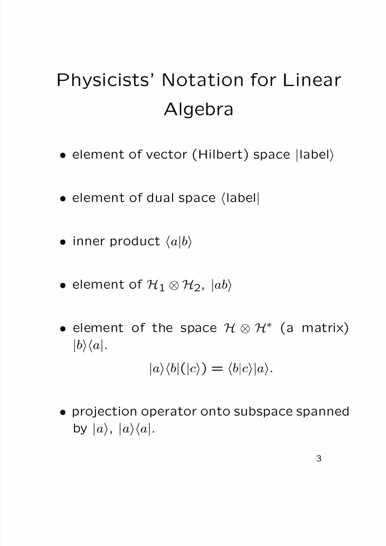
Physicists’ Notation for Linear
Algebra
• element of vector (Hilbert) space |label
• element of dual space label|
• inner product a|b
• element of H1 ⊗ H2, |ab
• element of the space H ⊗ H∗ (a matrix)
|ba|.
|a
b
|(
|c
) =
b
|c
|a
.
• projection operator onto subspace spanned
by |a, |aa|.
3

8/20/2019 Ottawa Foils
http://slidepdf.com/reader/full/ottawa-foils 4/44
Postulates of Quantum
Mechanics
• States form a Hilbert Space H,
• The evolution of an isolated system is gov-
erned by a unitary transformation on H:U (t, t) = exp(−iH(t − t)),
• Measurements are described by operators
acting on
H.
4
8/20/2019 Ottawa Foils
http://slidepdf.com/reader/full/ottawa-foils 5/44
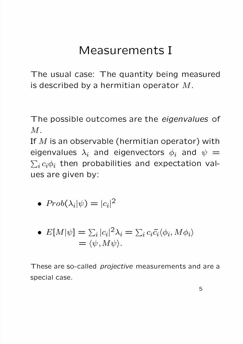
Measurements I
The usual case: The quantity being measured
is described by a hermitian operator M .
The possible outcomes are the eigenvalues of M .
If M is an observable (hermitian operator) with
eigenvalues λi and eigenvectors φi and ψ =i ciφi then probabilities and expectation val-
ues are given by:
• Prob(λi|ψ) = |ci|2
• E [M
|ψ] =
i
|ci
|2λi =
i cici
φi, M φi
= ψ , M ψ.
These are so-called projective measurements and are a
special case.
5
8/20/2019 Ottawa Foils
http://slidepdf.com/reader/full/ottawa-foils 6/44
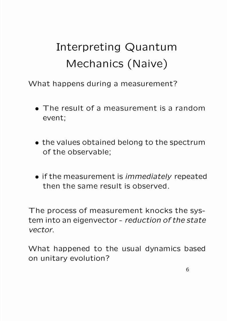
Interpreting Quantum
Mechanics (Naive)
What happens during a measurement?
• The result of a measurement is a random
event;
• the values obtained belong to the spectrum
of the observable;
• if the measurement is immediately repeated
then the same result is observed.
The process of measurement knocks the sys-
tem into an eigenvector - reduction of the state
vector .
What happened to the usual dynamics based
on unitary evolution?
6

8/20/2019 Ottawa Foils
http://slidepdf.com/reader/full/ottawa-foils 7/44
The “Theory” of Measurement
• Measurement is an interaction between
system and apparatus.
• Measurements do not uncover some pre-
existing physical property of a system. There
is no objective property being measured.
• The record or result of a measurement is
an objective property.
• Quantum mechanics is nothing more than
a set of rules to compute the outcome of physical tests to which a system may be
subjected.
7
8/20/2019 Ottawa Foils
http://slidepdf.com/reader/full/ottawa-foils 8/44
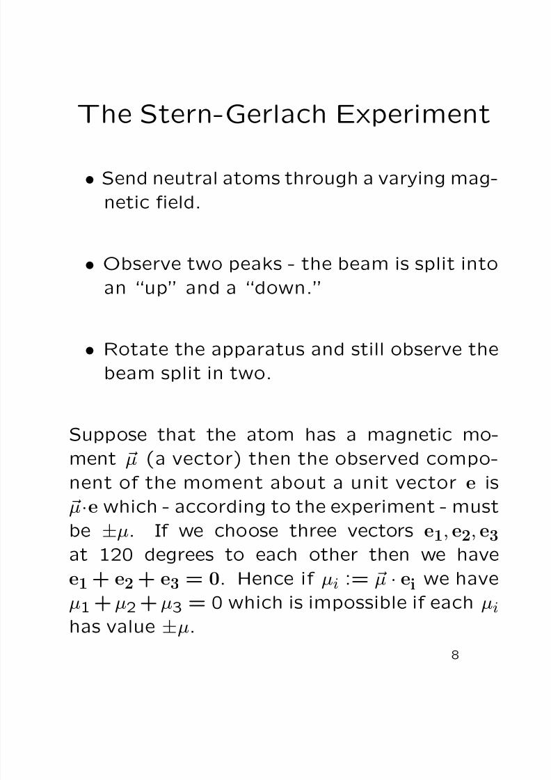
The Stern-Gerlach Experiment
• Send neutral atoms through a varying mag-
netic field.
• Observe two peaks - the beam is split intoan “up” and a “down.”
• Rotate the apparatus and still observe the
beam split in two.
Suppose that the atom has a magnetic mo-
ment µ (a vector) then the observed compo-
nent of the moment about a unit vector e is
µ·e which - according to the experiment - must
be
±µ. If we choose three vectors e1, e2, e3
at 120 degrees to each other then we have
e1 + e2 + e3 = 0. Hence if µi := µ · ei we have
µ1 + µ2 + µ3 = 0 which is impossible if each µi
has value ±µ.
8

8/20/2019 Ottawa Foils
http://slidepdf.com/reader/full/ottawa-foils 9/44
Composing Subsystems
A fundamental difference between classical and
quantum systems is:
we put systems together by tensor product in
quantum mechanics rather than by cartesian
product.
H = H1 ⊗ H2
This is the key to the power of quantum com-
puting: see various papers by Josza at
www.cs.bris.ac.uk/Research/QuantumComputing/
entanglement.html
9
8/20/2019 Ottawa Foils
http://slidepdf.com/reader/full/ottawa-foils 10/44
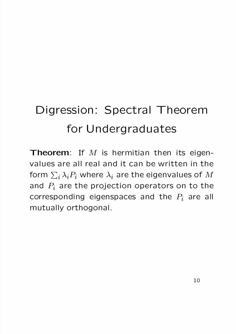
Digression: Spectral Theorem
for Undergraduates
Theorem: If M is hermitian then its eigen-
values are all real and it can be written in the
form
i λiP i where λi are the eigenvalues of M and P i are the projection operators on to the
corresponding eigenspaces and the P i are all
mutually orthogonal.
10

8/20/2019 Ottawa Foils
http://slidepdf.com/reader/full/ottawa-foils 11/44
Proof of the Spectral Theorem
Proof . The facts that the eigenvalues are all
real and that the P i are orthogonal are easy
to prove. For the main claim we proceed by
induction on the dimension d. The case d =
1 is trivial. Let λ be an eigenvalue of M , P
the projector onto its eigenspace and Q the
orthogonal projector to P . We have P + Q = I
and P Q = 0. Now clearly P M P = λP .
M = (P + Q)M (P + Q)
= P M P + QM Q + QM P + PMQ.
Now QM P = 0 and (P M Q)† = QM P = 0 so
P M Q = 0. Also QM Q is hermitian so by in-
ductive hypothesis it has the required form andfrom
M = λP + QM Q
we conclude.
11

8/20/2019 Ottawa Foils
http://slidepdf.com/reader/full/ottawa-foils 12/44
Density Matrices (Operators)
An alternative description of states and of the
postulates of quantum mechanics due to von
Neumann.
• Given ψ ∈ H we have a projection operator P ψ or |ψψ|. When a system is in the state
ψ we say that |ψψ| is the density matrix
of the system.
• A unitary operator U acts on |ψ by U |ψand hence it acts on |ψψ| by U |ψψ|U †.
• If M is an observable and P ψ is the density
matrix
– P r(λi|P ψ) = T r(P iP ψ)
– E [M |P ψ] = T r(M P ψ).
12

8/20/2019 Ottawa Foils
http://slidepdf.com/reader/full/ottawa-foils 13/44
Why bother with Density
Matrices I?
• Density matrices capture the notion of sta-
tistical mixture .
• Statistical mixture of states from H
ρ =m
j=1
p j|ψ jψ j|
where
j p j = 1.
• If all but one p j are zero then we have a
pure state otherwise a mixed state.
• Thus a density matrix can be seen as a
convex combination of projection opera-
tors corresponding to pure states.
13
8/20/2019 Ottawa Foils
http://slidepdf.com/reader/full/ottawa-foils 14/44
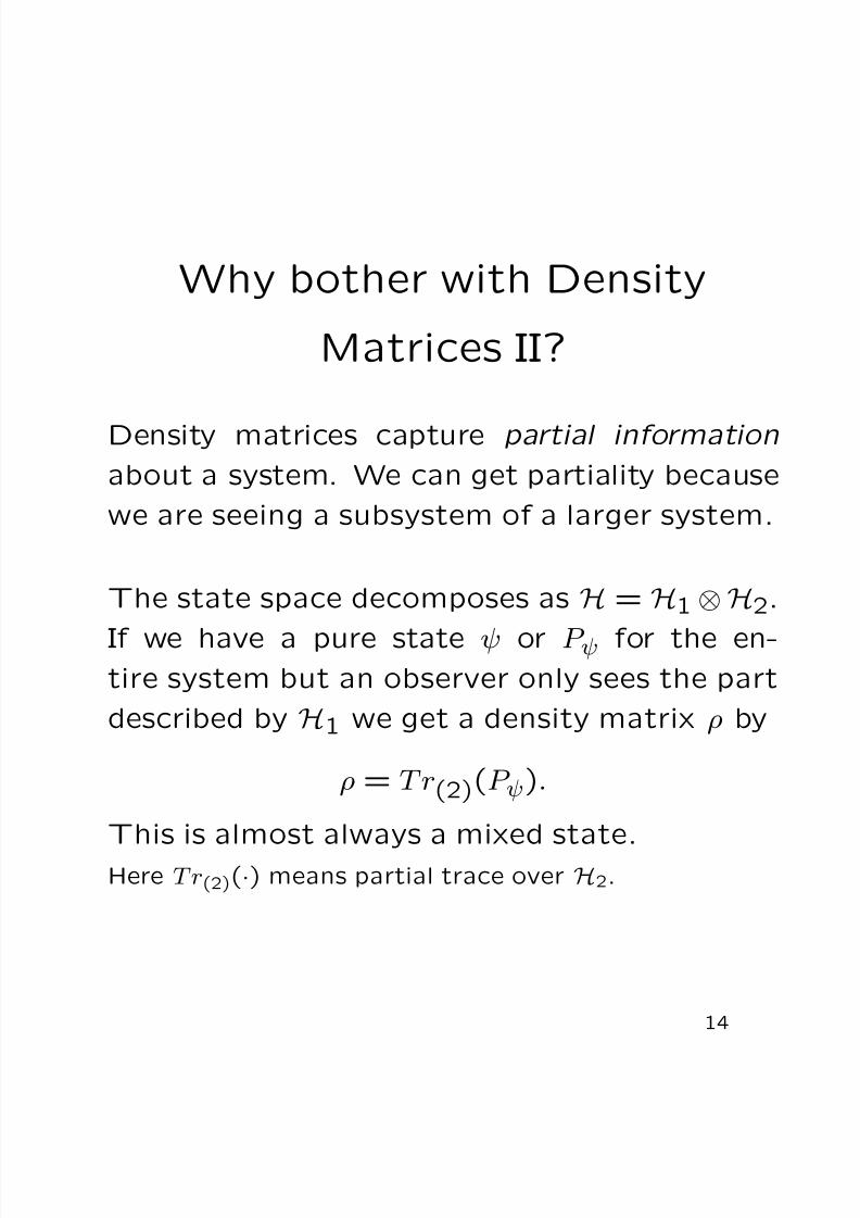
Why bother with Density
Matrices II?
Density matrices capture partial information
about a system. We can get partiality because
we are seeing a subsystem of a larger system.
The state space decomposes as H = H1 ⊗ H2.
If we have a pure state ψ or P ψ for the en-tire system but an observer only sees the part
described by H1 we get a density matrix ρ by
ρ = T r(2)(P ψ).
This is almost always a mixed state.
Here T r(2)(·) means partial trace over H2.
14
8/20/2019 Ottawa Foils
http://slidepdf.com/reader/full/ottawa-foils 15/44
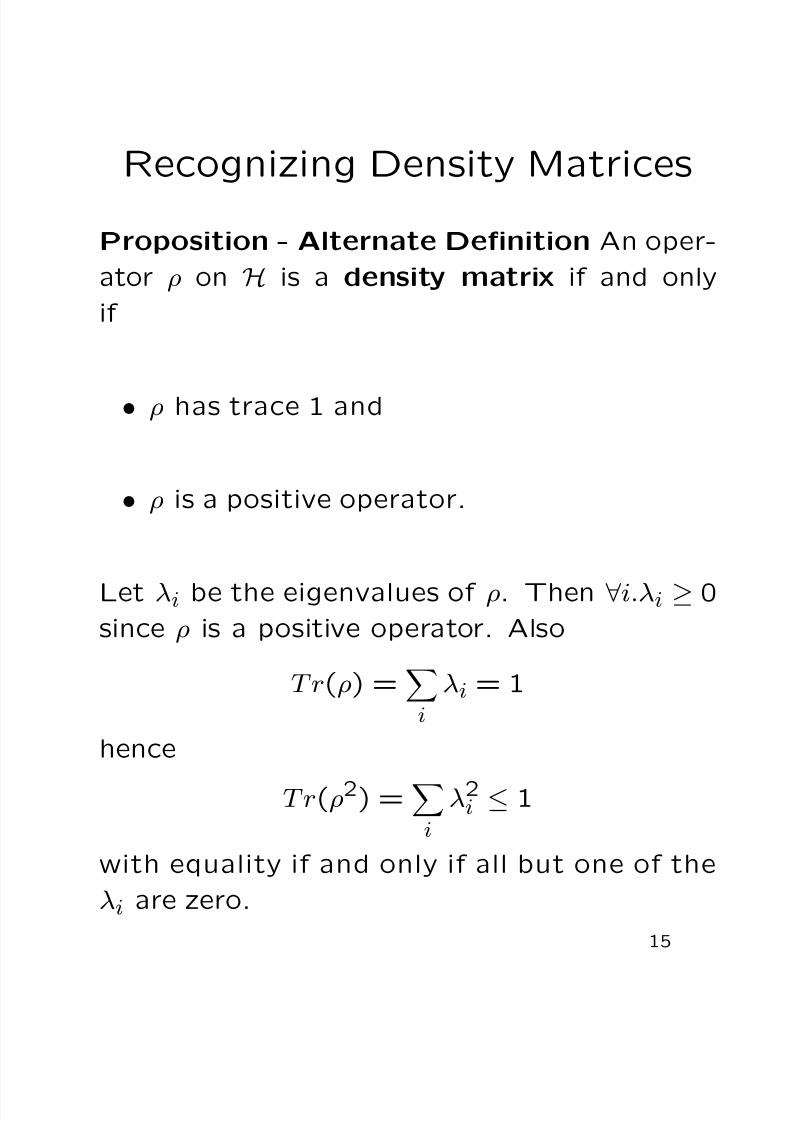
Recognizing Density Matrices
Proposition - Alternate Definition An oper-
ator ρ on H is a density matrix if and only
if
• ρ has trace 1 and
• ρ is a positive operator.
Let λi be the eigenvalues of ρ. Then ∀i.λi ≥ 0since ρ is a positive operator. Also
T r(ρ) =
i
λi = 1
hence
T r(ρ2) =
i
λ2i ≤ 1
with equality if and only if all but one of the
λi are zero.
15
8/20/2019 Ottawa Foils
http://slidepdf.com/reader/full/ottawa-foils 16/44
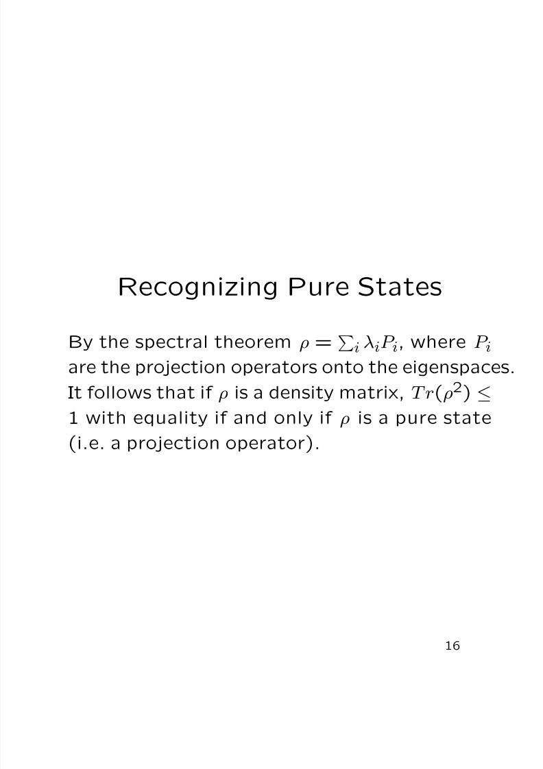
Recognizing Pure States
By the spectral theorem ρ =
i λiP i, where P i
are the projection operators onto the eigenspaces.
It follows that if ρ is a density matrix, T r(ρ2) ≤1 with equality if and only if ρ is a pure state
(i.e. a projection operator).
16

8/20/2019 Ottawa Foils
http://slidepdf.com/reader/full/ottawa-foils 17/44
Density matrices as probabilitydistributions
Note that a positive operator has non nega-
tive eigenvalues and trace 1 means that they
add up to 1. So by the spectral theorem suchan operator is a convex combination of projec-
tions operators. So
density matrices are “just” probability distribu-
tions on pure states?
No!
17

8/20/2019 Ottawa Foils
http://slidepdf.com/reader/full/ottawa-foils 18/44
Given a density matrix for a mixed state one
cannot recover a unique decomposition into
pure states.

8/20/2019 Ottawa Foils
http://slidepdf.com/reader/full/ottawa-foils 19/44
Mixtures vs Superpositions
A photon can be polarized so the state space
is a 2-dim Hilbert space. Consider the basis:
• | ↔: polarized along the x-axis
• | : polarized along the y-axis
A | ↔ photon will not get through a filter.
Such a photon will get through a filter oriented
at an angle of θ to the vertical with probability
proportional to sin2 θ.
18

8/20/2019 Ottawa Foils
http://slidepdf.com/reader/full/ottawa-foils 20/44
Mixtures vs Superpositions II
A photon can be in a superposed state, i.e. a
linear combination of basis states. For example
| = 1√
2[| ↔ + | ].
The density matrix for this pure state is1
2[| ↔↔ | + | ↔ |
+| ↔ | + | |]
19
8/20/2019 Ottawa Foils
http://slidepdf.com/reader/full/ottawa-foils 21/44
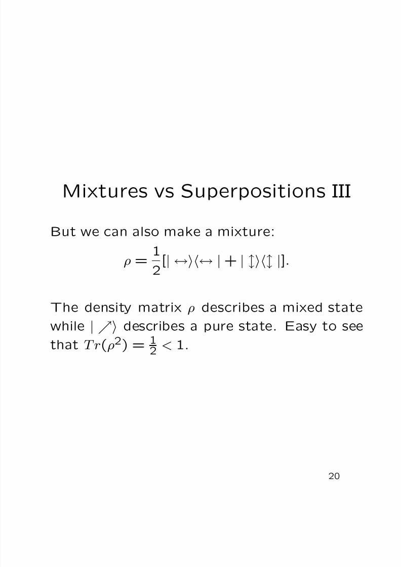
Mixtures vs Superpositions IIIBut we can also make a mixture:
ρ = 1
2[| ↔↔ | + | |].
The density matrix ρ describes a mixed state
while | describes a pure state. Easy to see
that T r(ρ2) = 12 < 1.
20

8/20/2019 Ottawa Foils
http://slidepdf.com/reader/full/ottawa-foils 22/44
What is the observable
difference?
With a polarizer aligned along the diagonal :
• All | photons get through
• Only half the ρ photons get through.
21

8/20/2019 Ottawa Foils
http://slidepdf.com/reader/full/ottawa-foils 23/44
How to make a mixed state I
Consider a two state system with the states
|0 and |1. We write |01 for |0⊗|1. Prepare
the EPR state
1
√ 2[
|00
− |11
]
or in terms of density matrices
1
2[|0000| − |1100| − |0011| + |1111|].
22
8/20/2019 Ottawa Foils
http://slidepdf.com/reader/full/ottawa-foils 24/44
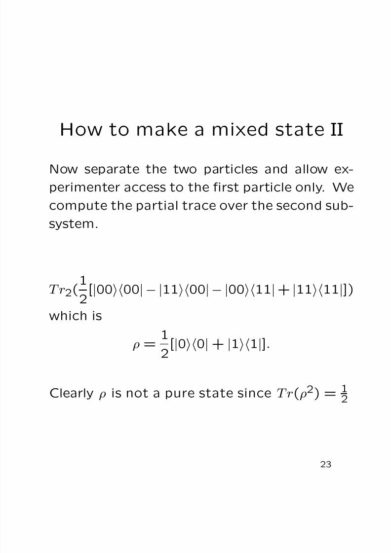
How to make a mixed state II
Now separate the two particles and allow ex-
perimenter access to the first particle only. Wecompute the partial trace over the second sub-
system.
T r2(
1
2[|0000| − |1100| − |0011| + |1111|])
which is
ρ = 1
2[|00| + |11|].
Clearly ρ is not a pure state since T r(ρ2) = 12
23
8/20/2019 Ottawa Foils
http://slidepdf.com/reader/full/ottawa-foils 25/44
Non-locality and Entanglement
A key idea due to Einstein, Podolsky and Rosen(1935) which was intended as an attack on
quantum mechanics. Turned out to be revo-
lutionary and led to the notion of non-locality
and entanglement.
A different manifestation of non locality was
discovered by Aharanov and Bohm in 1959 in
which electrons react to the presence of a mag-
netic field that is “far away.” [Don’t ask me
now!]
24
8/20/2019 Ottawa Foils
http://slidepdf.com/reader/full/ottawa-foils 26/44
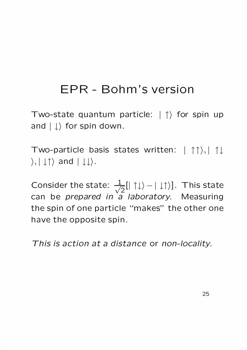
EPR - Bohm’s version
Two-state quantum particle:
| ↑ for spin up
and | ↓ for spin down.
Two-particle basis states written: | ↑↑, | ↑↓, | ↓↑ and | ↓↓.
Consider the state: 1√ 2[| ↑↓− | ↓↑]. This statecan be prepared in a laboratory . Measuring
the spin of one particle “makes” the other one
have the opposite spin.
This is action at a distance or non-locality .
25

8/20/2019 Ottawa Foils
http://slidepdf.com/reader/full/ottawa-foils 27/44
EPR - Consequences
Information is nonlocal , a quantum mechanical
state is nonlocal. We can substitute entangle-
ment for communication.
What EPR cannot be used for is superluminal
communication.
26

8/20/2019 Ottawa Foils
http://slidepdf.com/reader/full/ottawa-foils 28/44
Bell’s AnalysisAssuming that (local realism)
• there are objective values waiting to be
measured (realism)
• interactions are local.
There is an upper bound on the correlationsbetween distant independent measurements; no
quantum mechanical assumptions are needed
to derive this inequality. The Bell inequality
contradicts the predictions of quantum me-
chanics. Moreover, these inequalities are vio-lated experimentally . Thus local realism does
not hold in nature. Usually one keeps locality
of interaction and jettisons realism. [Bohm]
27

8/20/2019 Ottawa Foils
http://slidepdf.com/reader/full/ottawa-foils 29/44
Summary of Quantum States
• Pure quantum states can be superposed;linear structure
• States can be non local (entangled)
• States can be mixed
• Mixed states are described by density op-
erators.
28

8/20/2019 Ottawa Foils
http://slidepdf.com/reader/full/ottawa-foils 30/44
Evolution of States
Evolution of pure states is governed by unitary
operators.
U † = U −1
which implies
∀ψ, φU ψ , U φ = U †U ψ , φ = ψ, φ.
Typically U (t, t0) = exp −iH (t − t0) but we will
not worry about the detailed structure of evo-
lution operators.
On a density matrix ρ we have
ρ → ρ = U ρU †.
29
8/20/2019 Ottawa Foils
http://slidepdf.com/reader/full/ottawa-foils 31/44
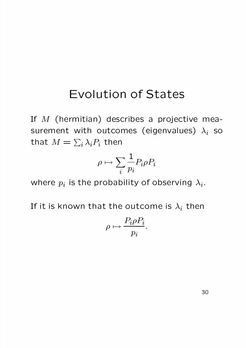
Evolution of States
If M (hermitian) describes a projective mea-surement with outcomes (eigenvalues) λi so
that M =
i λiP i then
ρ →
i
1
piP iρP i
where pi is the probability of observing λi.
If it is known that the outcome is λi then
ρ → P iρP i
pi.
30

8/20/2019 Ottawa Foils
http://slidepdf.com/reader/full/ottawa-foils 32/44
Evolution of States III
More generally, measurements are described by
positive operator-valued measures - the usual
projective measurements are a special case.
Outcomes labelled by µ ∈ {i , . . . , N }, to every
outcome we have an operator F µ. The trans-
formation of the density matrix is
ρ → ρ = 1
pµF µρF †µ.
Let E µ := F †µF µ; these are positive operators.
For a measurement they satisfy
µ E µ = I
and the probability of observing outcome µ is
T r(E µρ) = pµ as we had claimed.
31
8/20/2019 Ottawa Foils
http://slidepdf.com/reader/full/ottawa-foils 33/44
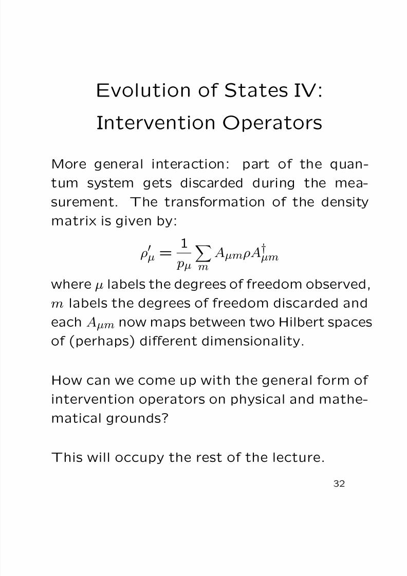
Evolution of States IV:Intervention Operators
More general interaction: part of the quan-
tum system gets discarded during the mea-
surement. The transformation of the densitymatrix is given by:
ρµ =
1
pµ
m
AµmρA†µm
where µ labels the degrees of freedom observed,
m labels the degrees of freedom discarded andeach Aµm now maps between two Hilbert spaces
of (perhaps) different dimensionality.
How can we come up with the general form of
intervention operators on physical and mathe-matical grounds?
This will occupy the rest of the lecture.
32

8/20/2019 Ottawa Foils
http://slidepdf.com/reader/full/ottawa-foils 34/44
Positive Operators
A : H −→ H is positive if ∀x ∈ H. x, Ax ≥ 0.
Implicit in this definition is the assumption that
x, Ax is always real; hence, all eigenvalues of A are real and A is hermitian.
33

8/20/2019 Ottawa Foils
http://slidepdf.com/reader/full/ottawa-foils 35/44
Positivity Abstractly
Any vector space V can be equipped with anotion of positivity. A subset C of V is calleda cone if
• x
∈ C implies that for any positive α, αx
∈C ,
• x, y ∈ C implies that x + y ∈ C and
• x and
−x both in C means that x = 0
We can define x ≥ 0 to mean x ∈ C and x ≥ y
to mean x − y ∈ C .
An ordered vector space is just a vector space
equipped with a cone.
Proposition: The collection of positive oper-ators in the vector space of linear operatorsforms a cone.
34
8/20/2019 Ottawa Foils
http://slidepdf.com/reader/full/ottawa-foils 36/44
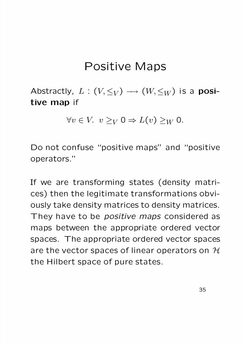
Positive Maps
Abstractly, L : (V, ≤V ) −→ (W, ≤W ) i s a posi-
tive map if
∀v ∈ V. v ≥V 0 ⇒ L(v) ≥W 0.
Do not confuse “positive maps” and “positive
operators.”
If we are transforming states (density matri-ces) then the legitimate transformations obvi-
ously take density matrices to density matrices.
They have to be positive maps considered as
maps between the appropriate ordered vector
spaces. The appropriate ordered vector spacesare the vector spaces of linear operators on Hthe Hilbert space of pure states.
35

8/20/2019 Ottawa Foils
http://slidepdf.com/reader/full/ottawa-foils 37/44
The problem with positive maps
Unfortunately the tensor product of two posi-
tive maps is not positive in general. We really
want this! If I can perform transformation T 1
on density matrix ρ1 and transformation T 2 on
density matrix ρ2
then I should be able to re-
gard ρ1 ⊗ ρ2 as a composite system and carry
out T 1 ⊗ T 2 on this system. We certainly want
this if, say, T 2 is the identity. But even when
T 2 is the identity this may fail!!
36

8/20/2019 Ottawa Foils
http://slidepdf.com/reader/full/ottawa-foils 38/44
Example of a “Bad” Positive
Map
Take H to be the two-dimensional Hilbert spacewith basis vectors |0 and |1, take T 1 to bethe map that transposes a density matrix over
H and T 2 the identity. The transpose map ispositive because it does not change any of theeigenvalues.
Consider the entangled state
1
√ 2[
|00
+
|11
]
with density matrix
1
2[|0000| + |0011| + |1100| + |1111|].
In matrix form this is:
1 0 0 10 0 0 00 0 0 01 0 0 1
37
8/20/2019 Ottawa Foils
http://slidepdf.com/reader/full/ottawa-foils 39/44
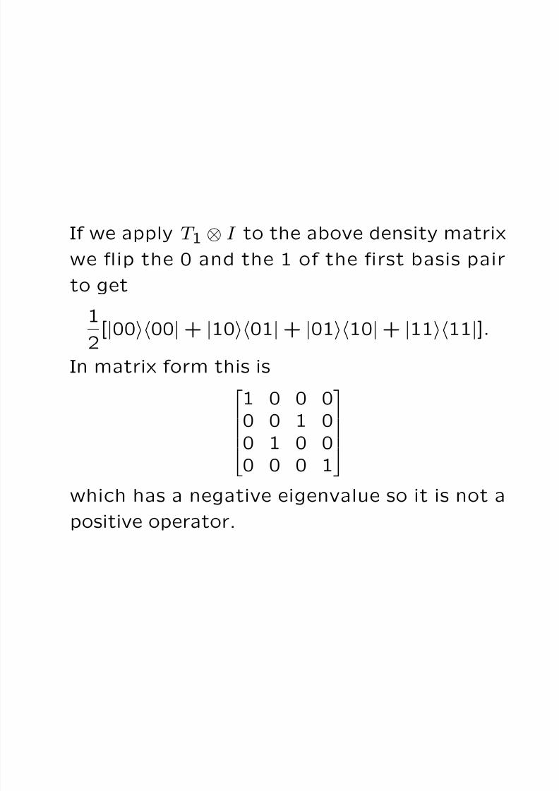
If we apply T 1 ⊗ I to the above density matrix
we flip the 0 and the 1 of the first basis pair
to get
1
2[|0000| + |1001| + |0110| + |1111|].
In matrix form this is
1 0 0 0
0 0 1 00 1 0 00 0 0 1
which has a negative eigenvalue so it is not a
positive operator.

8/20/2019 Ottawa Foils
http://slidepdf.com/reader/full/ottawa-foils 40/44
Completely Positive Maps
• Acompletely positive map K is a posi-
tive map such that for every identity map
I n : Cn −→ Cn the tensor product K ⊗ I n is
positive.
• The tensor of completely positive maps is
always a completely positive map.
38
8/20/2019 Ottawa Foils
http://slidepdf.com/reader/full/ottawa-foils 41/44
A Convenient(?) Category for
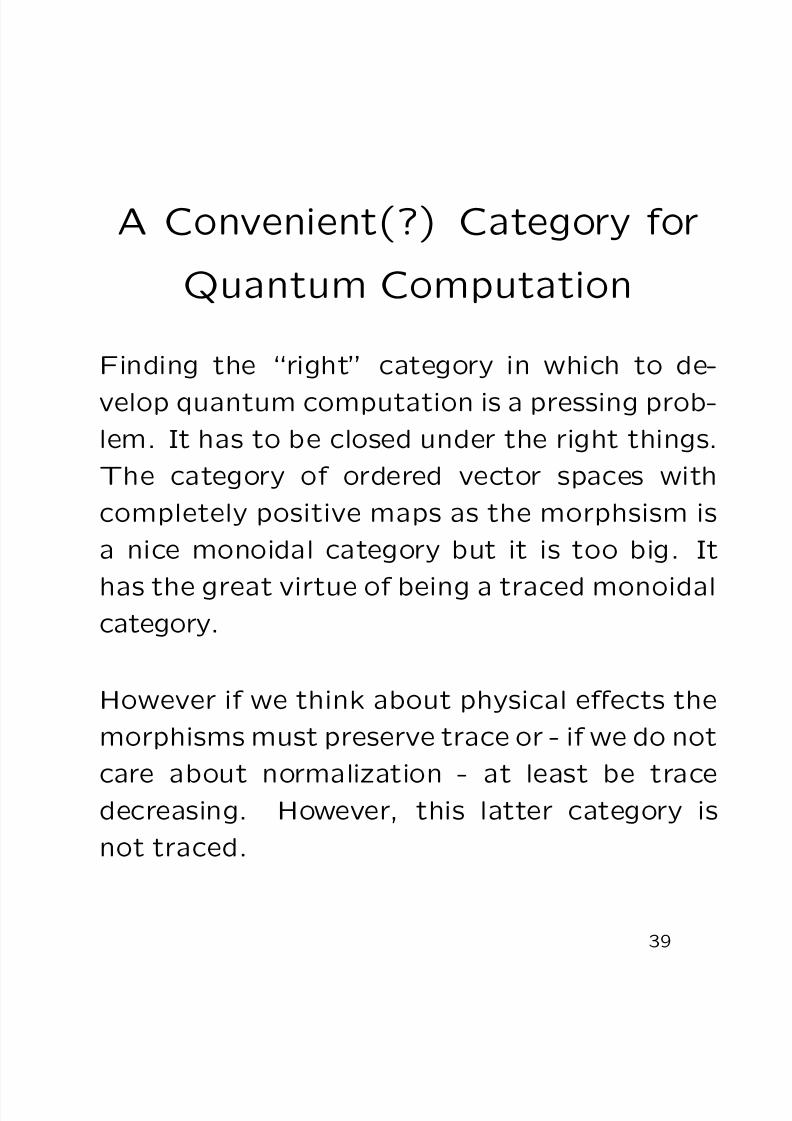
Quantum Computation
Finding the “right” category in which to de-
velop quantum computation is a pressing prob-
lem. It has to be closed under the right things.
The category of ordered vector spaces with
completely positive maps as the morphsism is
a nice monoidal category but it is too big. It
has the great virtue of being a traced monoidalcategory.
However if we think about physical effects the
morphisms must preserve trace or - if we do not
care about normalization - at least be tracedecreasing. However, this latter category is
not traced.
39

8/20/2019 Ottawa Foils
http://slidepdf.com/reader/full/ottawa-foils 42/44
The Kraus Representation
Theorem
The important result is the Kraus representa-
tion theorem (due to M.-D. Choi)
The general form for a completely positive map
E : B(H1) −→ B(H2) is
E (ρ) =m
AmρA†m
where the Am : H1 −→ H2.
Here B(H) is the Banach space of bounded
linear operators on H.
In other words: Completely positive maps andintervention operators are the same thing.
A more abstract version of this theorem was proved by Stinespring
in 1955.
40
8/20/2019 Ottawa Foils
http://slidepdf.com/reader/full/ottawa-foils 43/44
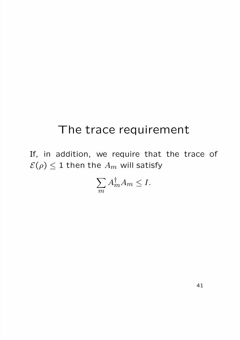
The trace requirement
If, in addition, we require that the trace of
E (ρ) ≤ 1 then the Am will satisfy
m
A†mAm ≤ I.
41

8/20/2019 Ottawa Foils
http://slidepdf.com/reader/full/ottawa-foils 44/44
Final Summary
• States are density matrices; i.e. positive
operators with trace 1.
• Physical transformations are trace preserv-
ing (decreasing) completely positive maps.
42