ORTEC · 2018-05-07 · ORTEC ® GammaVision® Gamma-Ray Spectrum Analysis and MCA Emulator for...
496
ORTEC ® GammaVision ® Gamma-Ray Spectrum Analysis and MCA Emulator for Microsoft ® Windows ® 7, 8.1, and 10 Professional A66-BW Software User’s Manual Software Version 8.1 Printed in U.S.A. ORTEC Part No. 783620 0917 Manual Revision L
Transcript of ORTEC · 2018-05-07 · ORTEC ® GammaVision® Gamma-Ray Spectrum Analysis and MCA Emulator for...

ORTEC
®
GammaVision®
Gamma-Ray Spectrum Analysis and MCA Emulatorfor Microsoft® Windows® 7, 8.1, and 10 Professional
A66-BWSoftware User’s Manual
Software Version 8.1
Printed in U.S.A. ORTEC Part No. 783620 0917Manual Revision L

Advanced Measurement Technology, Inc.a/k/a/ ORTEC®, a subsidiary of AMETEK®, Inc.
WARRANTY
ORTEC* DISCLAIMS ALL WARRANTIES OF ANY KIND, EITHER EXPRESSED ORIMPLIED, INCLUDING, BUT NOT LIMITED TO, THE IMPLIED WARRANTIES OFMERCHANTABILITY AND FITNESS FOR A PARTICULAR PURPOSE, NOTEXPRESSLY SET FORTH HEREIN. IN NO EVENT WILL ORTEC BE LIABLE FORINDIRECT, INCIDENTAL, SPECIAL, OR CONSEQUENTIAL DAMAGES,INCLUDING LOST PROFITS OR LOST SAVINGS, EVEN IF ORTEC HAS BEENADVISED OF THE POSSIBILITY OF SUCH DAMAGES RESULTING FROM THEUSE OF THESE DATA.
Copyright © 2017, Advanced Measurement Technology, Inc. All rights reserved.
*ORTEC® is a registered trademark of Advanced Measurement Technology, Inc. All other trademarks used herein are the property oftheir respective owners.
NOTICE OF PROPRIETARY PROPERTY —This document and the information contained in it are the proprietary property ofAMETEK Inc., ORTEC Business Unit. It may not be copied or used in any manner nor may any of the information in or upon it be usedfor any purpose without the express written consent of an authorized agent of AMETEK Inc., ORTEC Business Unit.

TABLE OF CONTENTS
1. INTRODUCTION. . . . . . . . . . . . . . . . . . . . . . . . . . . . . . . . . . . . . . . . . . . . . . . . . . . . . . . . . . . 11.1. General. . . . . . . . . . . . . . . . . . . . . . . . . . . . . . . . . . . . . . . . . . . . . . . . . . . . . . . . . . . . . . . . 1
1.1.1. Automation for High-Throughput Environments. . . . . . . . . . . . . . . . . . . . . . . . . 31.1.2. Analysis and Display Tools. . . . . . . . . . . . . . . . . . . . . . . . . . . . . . . . . . . . . . . . . . 3
1.2. MCA Emulation. . . . . . . . . . . . . . . . . . . . . . . . . . . . . . . . . . . . . . . . . . . . . . . . . . . . . . . . . 31.3. Computer Requirements and Operating System Cautions. . . . . . . . . . . . . . . . . . . . . . . . 51.4. MCB Support in GammaVision v8. . . . . . . . . . . . . . . . . . . . . . . . . . . . . . . . . . . . . . . . . . 51.5. Detector Security. . . . . . . . . . . . . . . . . . . . . . . . . . . . . . . . . . . . . . . . . . . . . . . . . . . . . . . . 51.6. List Mode Support. . . . . . . . . . . . . . . . . . . . . . . . . . . . . . . . . . . . . . . . . . . . . . . . . . . . . . . 5
2. INSTALLING GAMMAVISION. . . . . . . . . . . . . . . . . . . . . . . . . . . . . . . . . . . . . . . . . . . . . . . 72.1. Step 1: Installing CONNECTIONS.. . . . . . . . . . . . . . . . . . . . . . . . . . . . . . . . . . . . . . . . . . . 72.2. Step 2: Installing GammaVision.. . . . . . . . . . . . . . . . . . . . . . . . . . . . . . . . . . . . . . . . . . . 72.3. Step 3: Establishing Communication With Your ORTEC MCBs. . . . . . . . . . . . . . . . . . 9
2.3.1. Configuring a New Instrument.. . . . . . . . . . . . . . . . . . . . . . . . . . . . . . . . . . . . . . 102.3.2. Customizing ID Numbers and Descriptions. . . . . . . . . . . . . . . . . . . . . . . . . . . . 11
2.4. Caution: Running the MCB Configuration Program Can Affect Quality Assurance.. . 112.4.1. Confirming the MCB Identification to Maintain QA Integrity. . . . . . . . . . . . . . 132.4.2. Editing the MCB Configuration Command Line.. . . . . . . . . . . . . . . . . . . . . . . . 14
2.5. Product Registration. . . . . . . . . . . . . . . . . . . . . . . . . . . . . . . . . . . . . . . . . . . . . . . . . . . . 152.6. Enabling Additional ORTEC Device Drivers and Adding New MCBs. . . . . . . . . . . . . 16
3. GETTING STARTED — A GAMMAVISION TUTORIAL. . . . . . . . . . . . . . . . . . . . . . . . . 173.1. Introduction. . . . . . . . . . . . . . . . . . . . . . . . . . . . . . . . . . . . . . . . . . . . . . . . . . . . . . . . . . . 173.2. Starting GammaVision.. . . . . . . . . . . . . . . . . . . . . . . . . . . . . . . . . . . . . . . . . . . . . . . . . . 18
3.2.1. Recalling a Spectrum. . . . . . . . . . . . . . . . . . . . . . . . . . . . . . . . . . . . . . . . . . . . . . 193.2.2. The Simplest Way To Do An Analysis. . . . . . . . . . . . . . . . . . . . . . . . . . . . . . . . 203.2.3. Loading a Library. . . . . . . . . . . . . . . . . . . . . . . . . . . . . . . . . . . . . . . . . . . . . . . . . 223.2.4. Setting the Analysis Parameters. . . . . . . . . . . . . . . . . . . . . . . . . . . . . . . . . . . . . . 233.2.5. Energy Calibration. . . . . . . . . . . . . . . . . . . . . . . . . . . . . . . . . . . . . . . . . . . . . . . . 26
3.2.5.1. Auto Calibration. . . . . . . . . . . . . . . . . . . . . . . . . . . . . . . . . . . . . . . . . . 303.2.6. Efficiency Calibration. . . . . . . . . . . . . . . . . . . . . . . . . . . . . . . . . . . . . . . . . . . . . 303.2.7. Energy and Efficiency Calibration Using the Calibration Wizard. . . . . . . . . . . 333.2.8. Changing a Library.. . . . . . . . . . . . . . . . . . . . . . . . . . . . . . . . . . . . . . . . . . . . . . . 353.2.9. Detector Setup. . . . . . . . . . . . . . . . . . . . . . . . . . . . . . . . . . . . . . . . . . . . . . . . . . . 36
3.2.9.1. Conversion Gain. . . . . . . . . . . . . . . . . . . . . . . . . . . . . . . . . . . . . . . . . . 37
Installation — page 7Tutorial — page 17
iii

GammaVision® V8 (A66-BW) 783620L / 0917
3.2.9.2. Detectors Set Up Manually. . . . . . . . . . . . . . . . . . . . . . . . . . . . . . . . . . 383.2.9.3. Computer-Controlled Hardware Setup. . . . . . . . . . . . . . . . . . . . . . . . . 383.2.9.4. Amplifier Settings. . . . . . . . . . . . . . . . . . . . . . . . . . . . . . . . . . . . . . . . . 38
Automatic Optimization. . . . . . . . . . . . . . . . . . . . . . . . . . . . . . . . 39Adjusting Amplifier Gain. . . . . . . . . . . . . . . . . . . . . . . . . . . . . . . 39
4. DISPLAY FEATURES. . . . . . . . . . . . . . . . . . . . . . . . . . . . . . . . . . . . . . . . . . . . . . . . . . . . . . 434.1. Startup. . . . . . . . . . . . . . . . . . . . . . . . . . . . . . . . . . . . . . . . . . . . . . . . . . . . . . . . . . . . . . . 434.2. Spectrum Displays. . . . . . . . . . . . . . . . . . . . . . . . . . . . . . . . . . . . . . . . . . . . . . . . . . . . . . 464.3. The Toolbar. . . . . . . . . . . . . . . . . . . . . . . . . . . . . . . . . . . . . . . . . . . . . . . . . . . . . . . . . . . 474.4. Using the Mouse. . . . . . . . . . . . . . . . . . . . . . . . . . . . . . . . . . . . . . . . . . . . . . . . . . . . . . . 49
4.4.1. Moving the Marker with the Mouse. . . . . . . . . . . . . . . . . . . . . . . . . . . . . . . . . . 494.4.2. The Right-Mouse-Button Menu.. . . . . . . . . . . . . . . . . . . . . . . . . . . . . . . . . . . . . 494.4.3. Using the “Rubber Rectangle”. . . . . . . . . . . . . . . . . . . . . . . . . . . . . . . . . . . . . . . 504.4.4. Resizing and Moving the Full Spectrum View. . . . . . . . . . . . . . . . . . . . . . . . . . 50
4.5. Buttons and Boxes. . . . . . . . . . . . . . . . . . . . . . . . . . . . . . . . . . . . . . . . . . . . . . . . . . . . . . 504.6. Opening Files with Drag-and-Drop. . . . . . . . . . . . . . . . . . . . . . . . . . . . . . . . . . . . . . . . . 524.7. Associated Files. . . . . . . . . . . . . . . . . . . . . . . . . . . . . . . . . . . . . . . . . . . . . . . . . . . . . . . . 52
5. MENU COMMANDS. . . . . . . . . . . . . . . . . . . . . . . . . . . . . . . . . . . . . . . . . . . . . . . . . . . . . . . 535.1. File. . . . . . . . . . . . . . . . . . . . . . . . . . . . . . . . . . . . . . . . . . . . . . . . . . . . . . . . . . . . . . . . . . 56
5.1.1. Settings.... . . . . . . . . . . . . . . . . . . . . . . . . . . . . . . . . . . . . . . . . . . . . . . . . . . . . . . 565.1.1.1. General. . . . . . . . . . . . . . . . . . . . . . . . . . . . . . . . . . . . . . . . . . . . . . . . . . 56
Save File Format. . . . . . . . . . . . . . . . . . . . . . . . . . . . . . . . . . . . . . 57Ask On Save Options. . . . . . . . . . . . . . . . . . . . . . . . . . . . . . . . . . 58Sample Start/End Time. . . . . . . . . . . . . . . . . . . . . . . . . . . . . . . . . 58
5.1.1.2. Export.. . . . . . . . . . . . . . . . . . . . . . . . . . . . . . . . . . . . . . . . . . . . . . . . . . 58Arguments. . . . . . . . . . . . . . . . . . . . . . . . . . . . . . . . . . . . . . . . . . . 59Initial Directory.. . . . . . . . . . . . . . . . . . . . . . . . . . . . . . . . . . . . . . 60Run Options. . . . . . . . . . . . . . . . . . . . . . . . . . . . . . . . . . . . . . . . . 60Use DataMaster. . . . . . . . . . . . . . . . . . . . . . . . . . . . . . . . . . . . . . . 60
5.1.1.3. Import.. . . . . . . . . . . . . . . . . . . . . . . . . . . . . . . . . . . . . . . . . . . . . . . . . . 61Arguments:. . . . . . . . . . . . . . . . . . . . . . . . . . . . . . . . . . . . . . . . . . 61Initial Directory.. . . . . . . . . . . . . . . . . . . . . . . . . . . . . . . . . . . . . . 62Default. . . . . . . . . . . . . . . . . . . . . . . . . . . . . . . . . . . . . . . . . . . . . . 62Run Options. . . . . . . . . . . . . . . . . . . . . . . . . . . . . . . . . . . . . . . . . 62Use DataMaster. . . . . . . . . . . . . . . . . . . . . . . . . . . . . . . . . . . . . . . 62
5.1.1.4. Directories. . . . . . . . . . . . . . . . . . . . . . . . . . . . . . . . . . . . . . . . . . . . . . . 625.1.2. Recall.... . . . . . . . . . . . . . . . . . . . . . . . . . . . . . . . . . . . . . . . . . . . . . . . . . . . . . . . . 635.1.3. Save/Save As.... . . . . . . . . . . . . . . . . . . . . . . . . . . . . . . . . . . . . . . . . . . . . . . . . . . 645.1.4. Export.... . . . . . . . . . . . . . . . . . . . . . . . . . . . . . . . . . . . . . . . . . . . . . . . . . . . . . . . 65
iv

TABLE OF CONTENTS
5.1.5. Import.... . . . . . . . . . . . . . . . . . . . . . . . . . . . . . . . . . . . . . . . . . . . . . . . . . . . . . . . 655.1.6. Print.. . . . . . . . . . . . . . . . . . . . . . . . . . . . . . . . . . . . . . . . . . . . . . . . . . . . . . . . . . . 665.1.7. Compare..... . . . . . . . . . . . . . . . . . . . . . . . . . . . . . . . . . . . . . . . . . . . . . . . . . . . . . 66
5.1.7.1. Comparing ZDT Spectra with <Shift + F3>. . . . . . . . . . . . . . . . . . . . . 675.1.8. Save Plot.... . . . . . . . . . . . . . . . . . . . . . . . . . . . . . . . . . . . . . . . . . . . . . . . . . . . . . 685.1.9. Exit. . . . . . . . . . . . . . . . . . . . . . . . . . . . . . . . . . . . . . . . . . . . . . . . . . . . . . . . . . . . 695.1.10. About GammaVision..... . . . . . . . . . . . . . . . . . . . . . . . . . . . . . . . . . . . . . . . . . . 69
5.2. Acquire. . . . . . . . . . . . . . . . . . . . . . . . . . . . . . . . . . . . . . . . . . . . . . . . . . . . . . . . . . . . . . . 705.2.1. Acquisition Settings.... . . . . . . . . . . . . . . . . . . . . . . . . . . . . . . . . . . . . . . . . . . . . 70
5.2.1.1. Start/Save/Report. . . . . . . . . . . . . . . . . . . . . . . . . . . . . . . . . . . . . . . . . . 715.2.1.2. Ask on Start Options. . . . . . . . . . . . . . . . . . . . . . . . . . . . . . . . . . . . . . . 71
Sample Type Defaults. . . . . . . . . . . . . . . . . . . . . . . . . . . . . . . . . . 71Acquisition Presets. . . . . . . . . . . . . . . . . . . . . . . . . . . . . . . . . . . . 72Sample Description. . . . . . . . . . . . . . . . . . . . . . . . . . . . . . . . . . . . 72Sample Size. . . . . . . . . . . . . . . . . . . . . . . . . . . . . . . . . . . . . . . . . . 72Collection Date and Time. . . . . . . . . . . . . . . . . . . . . . . . . . . . . . . 72Sample Start/Stop Time. . . . . . . . . . . . . . . . . . . . . . . . . . . . . . . . 73
5.2.2. Start.. . . . . . . . . . . . . . . . . . . . . . . . . . . . . . . . . . . . . . . . . . . . . . . . . . . . . . . . . . . 735.2.3. Start/Save/Report. . . . . . . . . . . . . . . . . . . . . . . . . . . . . . . . . . . . . . . . . . . . . . . . . 735.2.4. Stop. . . . . . . . . . . . . . . . . . . . . . . . . . . . . . . . . . . . . . . . . . . . . . . . . . . . . . . . . . . . 735.2.5. Clear. . . . . . . . . . . . . . . . . . . . . . . . . . . . . . . . . . . . . . . . . . . . . . . . . . . . . . . . . . . 745.2.6. Copy to Buffer. . . . . . . . . . . . . . . . . . . . . . . . . . . . . . . . . . . . . . . . . . . . . . . . . . . 745.2.7. List Mode. . . . . . . . . . . . . . . . . . . . . . . . . . . . . . . . . . . . . . . . . . . . . . . . . . . . . . . 745.2.8. QA.. . . . . . . . . . . . . . . . . . . . . . . . . . . . . . . . . . . . . . . . . . . . . . . . . . . . . . . . . . . . 745.2.9. Download Spectra.... . . . . . . . . . . . . . . . . . . . . . . . . . . . . . . . . . . . . . . . . . . . . . . 745.2.10. ZDT Display Select. . . . . . . . . . . . . . . . . . . . . . . . . . . . . . . . . . . . . . . . . . . . . . 755.2.11. MCB Properties.... . . . . . . . . . . . . . . . . . . . . . . . . . . . . . . . . . . . . . . . . . . . . . . . 76
5.2.11.1. DSPEC-50. . . . . . . . . . . . . . . . . . . . . . . . . . . . . . . . . . . . . . . . . . . . . . 77Amplifier. . . . . . . . . . . . . . . . . . . . . . . . . . . . . . . . . . . . . . . . . . . . 77Amplifier 2. . . . . . . . . . . . . . . . . . . . . . . . . . . . . . . . . . . . . . . . . . 79Amplifier PRO. . . . . . . . . . . . . . . . . . . . . . . . . . . . . . . . . . . . . . . 80ADC . . . . . . . . . . . . . . . . . . . . . . . . . . . . . . . . . . . . . . . . . . . . . . . 83Stabilizer. . . . . . . . . . . . . . . . . . . . . . . . . . . . . . . . . . . . . . . . . . . . 84High Voltage. . . . . . . . . . . . . . . . . . . . . . . . . . . . . . . . . . . . . . . . . 85About.. . . . . . . . . . . . . . . . . . . . . . . . . . . . . . . . . . . . . . . . . . . . . . 86Status. . . . . . . . . . . . . . . . . . . . . . . . . . . . . . . . . . . . . . . . . . . . . . . 86Presets. . . . . . . . . . . . . . . . . . . . . . . . . . . . . . . . . . . . . . . . . . . . . . 87MDA Preset.. . . . . . . . . . . . . . . . . . . . . . . . . . . . . . . . . . . . . . . . . 89Nuclide Report Tab.. . . . . . . . . . . . . . . . . . . . . . . . . . . . . . . . . . . 90
5.2.11.2. Nuclide Report Calculations.. . . . . . . . . . . . . . . . . . . . . . . . . . . . . . . 925.2.11.3. Gain and Zero Stabilization.. . . . . . . . . . . . . . . . . . . . . . . . . . . . . . . . 93
v

GammaVision® V8 (A66-BW) 783620L / 0917
5.2.11.4. ZDT (Zero Dead Time) Mode. . . . . . . . . . . . . . . . . . . . . . . . . . . . . . . 94Choosing a ZDT Mode. . . . . . . . . . . . . . . . . . . . . . . . . . . . . . . . . 97The NORM_CORR Diagnostic Mode. . . . . . . . . . . . . . . . . . . . . 97More Information. . . . . . . . . . . . . . . . . . . . . . . . . . . . . . . . . . . . . 98
5.2.11.5. InSight Mode. . . . . . . . . . . . . . . . . . . . . . . . . . . . . . . . . . . . . . . . . . . . 98InSight Mode Controls. . . . . . . . . . . . . . . . . . . . . . . . . . . . . . . . . 98Mark Types. . . . . . . . . . . . . . . . . . . . . . . . . . . . . . . . . . . . . . . . . 100
5.2.11.6. Setting the Rise Time in Digital MCBs.. . . . . . . . . . . . . . . . . . . . . . 1025.3. Calibrate. . . . . . . . . . . . . . . . . . . . . . . . . . . . . . . . . . . . . . . . . . . . . . . . . . . . . . . . . . . . . 103
5.3.1. General Information, Cautions, and Tips.. . . . . . . . . . . . . . . . . . . . . . . . . . . . . 1035.3.1.1. For Best Calibration Results. . . . . . . . . . . . . . . . . . . . . . . . . . . . . . . . 104
5.3.2. Energy.... . . . . . . . . . . . . . . . . . . . . . . . . . . . . . . . . . . . . . . . . . . . . . . . . . . . . . . 1055.3.2.1. Introduction. . . . . . . . . . . . . . . . . . . . . . . . . . . . . . . . . . . . . . . . . . . . . 1055.3.2.2. Auto Calibration. . . . . . . . . . . . . . . . . . . . . . . . . . . . . . . . . . . . . . . . . 1065.3.2.3. Manual Calibration. . . . . . . . . . . . . . . . . . . . . . . . . . . . . . . . . . . . . . . 1075.3.2.4. Easy Recalibration Using An .ENT Table. . . . . . . . . . . . . . . . . . . . . 1115.3.2.5. Speeding Up Calibration with a Library. . . . . . . . . . . . . . . . . . . . . . . 1125.3.2.6. Other Sidebar Control Commands. . . . . . . . . . . . . . . . . . . . . . . . . . . 1135.3.2.7. Using Multiple Spectra for a Single Calibration.. . . . . . . . . . . . . . . . 113
5.3.3. Efficiency..... . . . . . . . . . . . . . . . . . . . . . . . . . . . . . . . . . . . . . . . . . . . . . . . . . . . 1145.3.3.1. Introduction. . . . . . . . . . . . . . . . . . . . . . . . . . . . . . . . . . . . . . . . . . . . . 1145.3.3.2. Interpolative Fit. . . . . . . . . . . . . . . . . . . . . . . . . . . . . . . . . . . . . . . . . . 1175.3.3.3. Linear Fit. . . . . . . . . . . . . . . . . . . . . . . . . . . . . . . . . . . . . . . . . . . . . . . 1185.3.3.4. Quadratic Fit. . . . . . . . . . . . . . . . . . . . . . . . . . . . . . . . . . . . . . . . . . . . 1185.3.3.5. Polynomial Fit. . . . . . . . . . . . . . . . . . . . . . . . . . . . . . . . . . . . . . . . . . . 1195.3.3.6. TCC Polynomial Fit.. . . . . . . . . . . . . . . . . . . . . . . . . . . . . . . . . . . . . . 1205.3.3.7. Performing the Efficiency Calibration. . . . . . . . . . . . . . . . . . . . . . . . 1205.3.3.8. Using The Library. . . . . . . . . . . . . . . . . . . . . . . . . . . . . . . . . . . . . . . . 1235.3.3.9. Automatic Efficiency Calibration. . . . . . . . . . . . . . . . . . . . . . . . . . . . 1255.3.3.10. Manual Calibration. . . . . . . . . . . . . . . . . . . . . . . . . . . . . . . . . . . . . . 1255.3.3.11. Other Efficiency Sidebar Control Commands.. . . . . . . . . . . . . . . . . 1255.3.3.12. Editing the Standard (.EFT) Table File. . . . . . . . . . . . . . . . . . . . . . . 1255.3.3.13. The Efficiency Graph Control Menu.. . . . . . . . . . . . . . . . . . . . . . . . 1285.3.3.14. The Efficiency Table Control Menu. . . . . . . . . . . . . . . . . . . . . . . . . 128
5.3.4. Description.... . . . . . . . . . . . . . . . . . . . . . . . . . . . . . . . . . . . . . . . . . . . . . . . . . . 1295.3.5. Recall Calibration.... . . . . . . . . . . . . . . . . . . . . . . . . . . . . . . . . . . . . . . . . . . . . . 1295.3.6. Save Calibration.... . . . . . . . . . . . . . . . . . . . . . . . . . . . . . . . . . . . . . . . . . . . . . . 1305.3.7. Print Calibration.... . . . . . . . . . . . . . . . . . . . . . . . . . . . . . . . . . . . . . . . . . . . . . . 1305.3.8. Calibration Wizard.... . . . . . . . . . . . . . . . . . . . . . . . . . . . . . . . . . . . . . . . . . . . . 132
5.3.8.1. Energy Calibration — Setting Up a New Calibration or Recalling fromFile.. . . . . . . . . . . . . . . . . . . . . . . . . . . . . . . . . . . . . . . . . . . . . . . 133
vi

TABLE OF CONTENTS
Create New. . . . . . . . . . . . . . . . . . . . . . . . . . . . . . . . . . . . . . . . . 133Read From File. . . . . . . . . . . . . . . . . . . . . . . . . . . . . . . . . . . . . . 134
5.3.8.2. Efficiency and Efficiency-plus-TCC Calibrations — Setting Up a NewCalibration or Recalling from File. . . . . . . . . . . . . . . . . . . . . . . 135Create New. . . . . . . . . . . . . . . . . . . . . . . . . . . . . . . . . . . . . . . . . 135Read From File — Efficiency.. . . . . . . . . . . . . . . . . . . . . . . . . . 139Read from File — TCC.. . . . . . . . . . . . . . . . . . . . . . . . . . . . . . . 139
5.3.8.3. Performing the New Energy Calibration. . . . . . . . . . . . . . . . . . . . . . . 1405.3.8.4. Performing the New Efficiency or Efficiency-plus-TCC Calibration
. . . . . . . . . . . . . . . . . . . . . . . . . . . . . . . . . . . . . . . . . . . . . . . . . . . 1415.3.8.5. Reviewing the Calibration Wizard Results. . . . . . . . . . . . . . . . . . . . . 141
5.4. Calculate.. . . . . . . . . . . . . . . . . . . . . . . . . . . . . . . . . . . . . . . . . . . . . . . . . . . . . . . . . . . . 1435.4.1. Settings.... . . . . . . . . . . . . . . . . . . . . . . . . . . . . . . . . . . . . . . . . . . . . . . . . . . . . . 1435.4.2. List Data Range.... . . . . . . . . . . . . . . . . . . . . . . . . . . . . . . . . . . . . . . . . . . . . . . . 1435.4.3. Peak Info.. . . . . . . . . . . . . . . . . . . . . . . . . . . . . . . . . . . . . . . . . . . . . . . . . . . . . . 144
5.4.3.1. Calculation. . . . . . . . . . . . . . . . . . . . . . . . . . . . . . . . . . . . . . . . . . . . . . 1455.4.4. Input Count Rate. . . . . . . . . . . . . . . . . . . . . . . . . . . . . . . . . . . . . . . . . . . . . . . . 1475.4.5. Sum. . . . . . . . . . . . . . . . . . . . . . . . . . . . . . . . . . . . . . . . . . . . . . . . . . . . . . . . . . . 1475.4.6. Smooth. . . . . . . . . . . . . . . . . . . . . . . . . . . . . . . . . . . . . . . . . . . . . . . . . . . . . . . . 1485.4.7. Strip.... . . . . . . . . . . . . . . . . . . . . . . . . . . . . . . . . . . . . . . . . . . . . . . . . . . . . . . . . 148
5.5. Analyze.. . . . . . . . . . . . . . . . . . . . . . . . . . . . . . . . . . . . . . . . . . . . . . . . . . . . . . . . . . . . . 1495.5.1. Settings. . . . . . . . . . . . . . . . . . . . . . . . . . . . . . . . . . . . . . . . . . . . . . . . . . . . . . . . 150
5.5.1.1. Sample Type.... . . . . . . . . . . . . . . . . . . . . . . . . . . . . . . . . . . . . . . . . . . 150Sample Tab. . . . . . . . . . . . . . . . . . . . . . . . . . . . . . . . . . . . . . . . . 150System Tab. . . . . . . . . . . . . . . . . . . . . . . . . . . . . . . . . . . . . . . . . 152Decay Tab. . . . . . . . . . . . . . . . . . . . . . . . . . . . . . . . . . . . . . . . . . 155Report Tab.. . . . . . . . . . . . . . . . . . . . . . . . . . . . . . . . . . . . . . . . . 156Analysis Tab. . . . . . . . . . . . . . . . . . . . . . . . . . . . . . . . . . . . . . . . 159Corrections Tab.. . . . . . . . . . . . . . . . . . . . . . . . . . . . . . . . . . . . . 162Isotopes Tab. . . . . . . . . . . . . . . . . . . . . . . . . . . . . . . . . . . . . . . . 164Uncertainties Tab. . . . . . . . . . . . . . . . . . . . . . . . . . . . . . . . . . . . 165
5.5.1.2. Report Generator. . . . . . . . . . . . . . . . . . . . . . . . . . . . . . . . . . . . . . . . . 1665.5.1.3. Attenuation Coefficients. . . . . . . . . . . . . . . . . . . . . . . . . . . . . . . . . . . 166
Coefficient Table.. . . . . . . . . . . . . . . . . . . . . . . . . . . . . . . . . . . . 166Calculate from Spectra. . . . . . . . . . . . . . . . . . . . . . . . . . . . . . . . 171
5.5.1.4. Geometry Correction. . . . . . . . . . . . . . . . . . . . . . . . . . . . . . . . . . . . . . 173Automatic Calculation. . . . . . . . . . . . . . . . . . . . . . . . . . . . . . . . 173Manual Calculation. . . . . . . . . . . . . . . . . . . . . . . . . . . . . . . . . . . 173Editing the Geometry Correction Table. . . . . . . . . . . . . . . . . . . 173
5.5.1.5. Peak Background Correction.. . . . . . . . . . . . . . . . . . . . . . . . . . . . . . . 174Create PBC.... . . . . . . . . . . . . . . . . . . . . . . . . . . . . . . . . . . . . . . . 175
vii

GammaVision® V8 (A66-BW) 783620L / 0917
Select PBC.... . . . . . . . . . . . . . . . . . . . . . . . . . . . . . . . . . . . . . . . 175Edit PBC..... . . . . . . . . . . . . . . . . . . . . . . . . . . . . . . . . . . . . . . . . 175Print PBC.... . . . . . . . . . . . . . . . . . . . . . . . . . . . . . . . . . . . . . . . . 180
5.5.1.6. Average Energy. . . . . . . . . . . . . . . . . . . . . . . . . . . . . . . . . . . . . . . . . . 180Average Energy Sidebar Control Menu. . . . . . . . . . . . . . . . . . . 182Average Energy Table Control Menu.. . . . . . . . . . . . . . . . . . . . 183
5.5.1.7. Iodine Equivalence. . . . . . . . . . . . . . . . . . . . . . . . . . . . . . . . . . . . . . . 183Iodine Equivalence Sidebar Control Menu. . . . . . . . . . . . . . . . 184Iodine Equivalence Table Control Menu. . . . . . . . . . . . . . . . . . 184
5.5.1.8. DAC (MPC). . . . . . . . . . . . . . . . . . . . . . . . . . . . . . . . . . . . . . . . . . . . . 184DAC (MPC) Sidebar Control Menu. . . . . . . . . . . . . . . . . . . . . . 185DAC (MPC) Table Control Menu. . . . . . . . . . . . . . . . . . . . . . . 186
5.5.1.9. Gamma Total..... . . . . . . . . . . . . . . . . . . . . . . . . . . . . . . . . . . . . . . . . . 186Output File Naming Convention. . . . . . . . . . . . . . . . . . . . . . . . 188Hardware and Analysis Configuration. . . . . . . . . . . . . . . . . . . . 188Configuring and Generating the Gamma Total Reports.. . . . . . 189
5.5.2. Peak Search.. . . . . . . . . . . . . . . . . . . . . . . . . . . . . . . . . . . . . . . . . . . . . . . . . . . . 1915.5.3. ROI Report.... . . . . . . . . . . . . . . . . . . . . . . . . . . . . . . . . . . . . . . . . . . . . . . . . . . 1915.5.4. Entire Spectrum in Memory.... . . . . . . . . . . . . . . . . . . . . . . . . . . . . . . . . . . . . . 1935.5.5. Spectrum on Disk.... . . . . . . . . . . . . . . . . . . . . . . . . . . . . . . . . . . . . . . . . . . . . . 1935.5.6. Display Analysis Results..... . . . . . . . . . . . . . . . . . . . . . . . . . . . . . . . . . . . . . . . 194
5.5.6.1. Analysis Sidebar. . . . . . . . . . . . . . . . . . . . . . . . . . . . . . . . . . . . . . . . . 1955.5.6.2. Analysis Results Spectrum Window. . . . . . . . . . . . . . . . . . . . . . . . . . 196
Plot Absolute Residuals/Plot Relative Residuals. . . . . . . . . . . . 196Zoom In. . . . . . . . . . . . . . . . . . . . . . . . . . . . . . . . . . . . . . . . . . . . 196Zoom Out. . . . . . . . . . . . . . . . . . . . . . . . . . . . . . . . . . . . . . . . . . 197Undo Zoom In. . . . . . . . . . . . . . . . . . . . . . . . . . . . . . . . . . . . . . . 197Full View.. . . . . . . . . . . . . . . . . . . . . . . . . . . . . . . . . . . . . . . . . . 197Mark ROI. . . . . . . . . . . . . . . . . . . . . . . . . . . . . . . . . . . . . . . . . . 197Clear Active ROI.. . . . . . . . . . . . . . . . . . . . . . . . . . . . . . . . . . . . 197Show ROI Bars. . . . . . . . . . . . . . . . . . . . . . . . . . . . . . . . . . . . . . 197Peak Info. . . . . . . . . . . . . . . . . . . . . . . . . . . . . . . . . . . . . . . . . . . 198Show Hover Window. . . . . . . . . . . . . . . . . . . . . . . . . . . . . . . . . 198Sum Spectrum. . . . . . . . . . . . . . . . . . . . . . . . . . . . . . . . . . . . . . . 198Print Graph. . . . . . . . . . . . . . . . . . . . . . . . . . . . . . . . . . . . . . . . . 199Properties.. . . . . . . . . . . . . . . . . . . . . . . . . . . . . . . . . . . . . . . . . . 199
5.5.6.3. Analysis Results Table. . . . . . . . . . . . . . . . . . . . . . . . . . . . . . . . . . . . 2005.5.7. Interactive in Viewed Area.... . . . . . . . . . . . . . . . . . . . . . . . . . . . . . . . . . . . . . . 203
5.6. Library. . . . . . . . . . . . . . . . . . . . . . . . . . . . . . . . . . . . . . . . . . . . . . . . . . . . . . . . . . . . . . 2065.6.1. Select Peak..... . . . . . . . . . . . . . . . . . . . . . . . . . . . . . . . . . . . . . . . . . . . . . . . . . . 2075.6.2. Select File.... . . . . . . . . . . . . . . . . . . . . . . . . . . . . . . . . . . . . . . . . . . . . . . . . . . . 207
viii

TABLE OF CONTENTS
5.6.3. Edit..... . . . . . . . . . . . . . . . . . . . . . . . . . . . . . . . . . . . . . . . . . . . . . . . . . . . . . . . . 2085.6.3.1. Copying Nuclides From Library to Library. . . . . . . . . . . . . . . . . . . . 2095.6.3.2. Creating a New Library Manually.. . . . . . . . . . . . . . . . . . . . . . . . . . . 2105.6.3.3. Editing Library List Nuclides. . . . . . . . . . . . . . . . . . . . . . . . . . . . . . . 211
Manually Adding Nuclides. . . . . . . . . . . . . . . . . . . . . . . . . . . . . 212Deleting Nuclides from the Library. . . . . . . . . . . . . . . . . . . . . . 212Rearranging the Library List.. . . . . . . . . . . . . . . . . . . . . . . . . . . 212Editing Nuclide Peaks.. . . . . . . . . . . . . . . . . . . . . . . . . . . . . . . . 213Adding Nuclide Peaks.. . . . . . . . . . . . . . . . . . . . . . . . . . . . . . . . 213Rearranging the Peak List.. . . . . . . . . . . . . . . . . . . . . . . . . . . . . 214
5.6.3.4. Saving or Canceling Changes and Closing. . . . . . . . . . . . . . . . . . . . . 2145.6.4. List.... . . . . . . . . . . . . . . . . . . . . . . . . . . . . . . . . . . . . . . . . . . . . . . . . . . . . . . . . . 214
5.7. Services. . . . . . . . . . . . . . . . . . . . . . . . . . . . . . . . . . . . . . . . . . . . . . . . . . . . . . . . . . . . . 2155.7.1. JOB Control..... . . . . . . . . . . . . . . . . . . . . . . . . . . . . . . . . . . . . . . . . . . . . . . . . . 215
5.7.1.1. Editing a .JOB File. . . . . . . . . . . . . . . . . . . . . . . . . . . . . . . . . . . . . . . 2155.7.2. Sample Description.... . . . . . . . . . . . . . . . . . . . . . . . . . . . . . . . . . . . . . . . . . . . . 2165.7.3. Menu Passwords.... . . . . . . . . . . . . . . . . . . . . . . . . . . . . . . . . . . . . . . . . . . . . . . 2175.7.4. Lock/Unlock Detectors.... . . . . . . . . . . . . . . . . . . . . . . . . . . . . . . . . . . . . . . . . . 2185.7.5. Edit Detector List.... . . . . . . . . . . . . . . . . . . . . . . . . . . . . . . . . . . . . . . . . . . . . . 219
5.8. ROI. . . . . . . . . . . . . . . . . . . . . . . . . . . . . . . . . . . . . . . . . . . . . . . . . . . . . . . . . . . . . . . . . 2215.8.1. Off.. . . . . . . . . . . . . . . . . . . . . . . . . . . . . . . . . . . . . . . . . . . . . . . . . . . . . . . . . . . 2215.8.2. Mark. . . . . . . . . . . . . . . . . . . . . . . . . . . . . . . . . . . . . . . . . . . . . . . . . . . . . . . . . . 2215.8.3. UnMark.. . . . . . . . . . . . . . . . . . . . . . . . . . . . . . . . . . . . . . . . . . . . . . . . . . . . . . . 2215.8.4. Mark Peak.. . . . . . . . . . . . . . . . . . . . . . . . . . . . . . . . . . . . . . . . . . . . . . . . . . . . . 2225.8.5. Clear. . . . . . . . . . . . . . . . . . . . . . . . . . . . . . . . . . . . . . . . . . . . . . . . . . . . . . . . . . 2225.8.6. Clear All. . . . . . . . . . . . . . . . . . . . . . . . . . . . . . . . . . . . . . . . . . . . . . . . . . . . . . . 2225.8.7. Auto Clear.. . . . . . . . . . . . . . . . . . . . . . . . . . . . . . . . . . . . . . . . . . . . . . . . . . . . . 2225.8.8. Save File.... . . . . . . . . . . . . . . . . . . . . . . . . . . . . . . . . . . . . . . . . . . . . . . . . . . . . 2225.8.9. Recall File.... . . . . . . . . . . . . . . . . . . . . . . . . . . . . . . . . . . . . . . . . . . . . . . . . . . . 223
5.9. Display. . . . . . . . . . . . . . . . . . . . . . . . . . . . . . . . . . . . . . . . . . . . . . . . . . . . . . . . . . . . . . 2235.9.1. Detector.... . . . . . . . . . . . . . . . . . . . . . . . . . . . . . . . . . . . . . . . . . . . . . . . . . . . . . 2235.9.2. Detector/Buffer.. . . . . . . . . . . . . . . . . . . . . . . . . . . . . . . . . . . . . . . . . . . . . . . . . 2245.9.3. Select Spectrum. . . . . . . . . . . . . . . . . . . . . . . . . . . . . . . . . . . . . . . . . . . . . . . . . 2245.9.4. Logarithmic. . . . . . . . . . . . . . . . . . . . . . . . . . . . . . . . . . . . . . . . . . . . . . . . . . . . 2245.9.5. Automatic. . . . . . . . . . . . . . . . . . . . . . . . . . . . . . . . . . . . . . . . . . . . . . . . . . . . . . 2245.9.6. Baseline Zoom. . . . . . . . . . . . . . . . . . . . . . . . . . . . . . . . . . . . . . . . . . . . . . . . . . 2245.9.7. Zoom In. . . . . . . . . . . . . . . . . . . . . . . . . . . . . . . . . . . . . . . . . . . . . . . . . . . . . . . 2255.9.8. Zoom Out. . . . . . . . . . . . . . . . . . . . . . . . . . . . . . . . . . . . . . . . . . . . . . . . . . . . . . 2255.9.9. Center. . . . . . . . . . . . . . . . . . . . . . . . . . . . . . . . . . . . . . . . . . . . . . . . . . . . . . . . . 2255.9.10. Full View. . . . . . . . . . . . . . . . . . . . . . . . . . . . . . . . . . . . . . . . . . . . . . . . . . . . . 2255.9.11. Isotope Markers. . . . . . . . . . . . . . . . . . . . . . . . . . . . . . . . . . . . . . . . . . . . . . . . 225
ix

GammaVision® V8 (A66-BW) 783620L / 0917
5.9.12. Preferences..... . . . . . . . . . . . . . . . . . . . . . . . . . . . . . . . . . . . . . . . . . . . . . . . . . 2275.9.12.1. Points/Fill ROI/Fill All. . . . . . . . . . . . . . . . . . . . . . . . . . . . . . . . . . . 2275.9.12.2. Spectrum Colors.... . . . . . . . . . . . . . . . . . . . . . . . . . . . . . . . . . . . . . . 2275.9.12.3. Peak Info Font/Color. . . . . . . . . . . . . . . . . . . . . . . . . . . . . . . . . . . . . 228
5.10. Window. . . . . . . . . . . . . . . . . . . . . . . . . . . . . . . . . . . . . . . . . . . . . . . . . . . . . . . . . . . . 2285.11. Right-Mouse-Button (Context) Menu. . . . . . . . . . . . . . . . . . . . . . . . . . . . . . . . . . . . . 229
5.11.1. Start.. . . . . . . . . . . . . . . . . . . . . . . . . . . . . . . . . . . . . . . . . . . . . . . . . . . . . . . . . 2295.11.2. Stop. . . . . . . . . . . . . . . . . . . . . . . . . . . . . . . . . . . . . . . . . . . . . . . . . . . . . . . . . . 2295.11.3. Clear. . . . . . . . . . . . . . . . . . . . . . . . . . . . . . . . . . . . . . . . . . . . . . . . . . . . . . . . . 2295.11.4. Copy to Buffer. . . . . . . . . . . . . . . . . . . . . . . . . . . . . . . . . . . . . . . . . . . . . . . . . 2295.11.5. Zoom In. . . . . . . . . . . . . . . . . . . . . . . . . . . . . . . . . . . . . . . . . . . . . . . . . . . . . . 2295.11.6. Zoom Out. . . . . . . . . . . . . . . . . . . . . . . . . . . . . . . . . . . . . . . . . . . . . . . . . . . . . 2295.11.7. Undo Zoom In. . . . . . . . . . . . . . . . . . . . . . . . . . . . . . . . . . . . . . . . . . . . . . . . . 2305.11.8. Mark ROI. . . . . . . . . . . . . . . . . . . . . . . . . . . . . . . . . . . . . . . . . . . . . . . . . . . . . 2305.11.9. Clear ROI. . . . . . . . . . . . . . . . . . . . . . . . . . . . . . . . . . . . . . . . . . . . . . . . . . . . . 2305.11.10. Peak Info.. . . . . . . . . . . . . . . . . . . . . . . . . . . . . . . . . . . . . . . . . . . . . . . . . . . . 2305.11.11. Input Count Rate. . . . . . . . . . . . . . . . . . . . . . . . . . . . . . . . . . . . . . . . . . . . . . 2305.11.12. Sum. . . . . . . . . . . . . . . . . . . . . . . . . . . . . . . . . . . . . . . . . . . . . . . . . . . . . . . . . 2305.11.13. MCB Properties.... . . . . . . . . . . . . . . . . . . . . . . . . . . . . . . . . . . . . . . . . . . . . . 230
6. ANALYSIS METHODS. . . . . . . . . . . . . . . . . . . . . . . . . . . . . . . . . . . . . . . . . . . . . . . . . . . . 2316.1. General. . . . . . . . . . . . . . . . . . . . . . . . . . . . . . . . . . . . . . . . . . . . . . . . . . . . . . . . . . . . . . 2316.2. The Analysis Engines. . . . . . . . . . . . . . . . . . . . . . . . . . . . . . . . . . . . . . . . . . . . . . . . . . 231
6.2.1. Analysis Engine Options. . . . . . . . . . . . . . . . . . . . . . . . . . . . . . . . . . . . . . . . . . 2316.2.1.1. WAN32. . . . . . . . . . . . . . . . . . . . . . . . . . . . . . . . . . . . . . . . . . . . . . . . 2316.2.1.2. GAM32. . . . . . . . . . . . . . . . . . . . . . . . . . . . . . . . . . . . . . . . . . . . . . . . 2326.2.1.3. NPP32. . . . . . . . . . . . . . . . . . . . . . . . . . . . . . . . . . . . . . . . . . . . . . . . . 2326.2.1.4. ENV32 and NAI32. . . . . . . . . . . . . . . . . . . . . . . . . . . . . . . . . . . . . . . 2326.2.1.5. ROI32.. . . . . . . . . . . . . . . . . . . . . . . . . . . . . . . . . . . . . . . . . . . . . . . . . 233
ROI Analysis. . . . . . . . . . . . . . . . . . . . . . . . . . . . . . . . . . . . . . . . 233Additional Considerations. . . . . . . . . . . . . . . . . . . . . . . . . . . . . 234
6.2.2. Selecting an Analysis Engine — Decision Matrix. . . . . . . . . . . . . . . . . . . . . . 2356.2.2.1. Guidelines for Selecting an Analysis Engine. . . . . . . . . . . . . . . . . . . 236
6.2.3. Library Reduction Based on Nuclide Rejection (ENV32, GAM32 and NAI32Analysis Engines Only). . . . . . . . . . . . . . . . . . . . . . . . . . . . . . . . . . . . . . . . . . . 2366.2.3.1. Library Reduction based on Peak Order. . . . . . . . . . . . . . . . . . . . . . . 2366.2.3.2. Library Reduction Based on Key Line and Fraction Limit Tests. . . . 237
6.3. Calculation Details for Peaks.. . . . . . . . . . . . . . . . . . . . . . . . . . . . . . . . . . . . . . . . . . . . 2386.3.1. Background Calculation Methods. . . . . . . . . . . . . . . . . . . . . . . . . . . . . . . . . . . 238
6.3.1.1. Automatic.. . . . . . . . . . . . . . . . . . . . . . . . . . . . . . . . . . . . . . . . . . . . . . 2386.3.1.2. X-Point Average. . . . . . . . . . . . . . . . . . . . . . . . . . . . . . . . . . . . . . . . . 240
x

TABLE OF CONTENTS
6.3.1.3. X.X * FWHM. . . . . . . . . . . . . . . . . . . . . . . . . . . . . . . . . . . . . . . . . . . 2406.3.1.4. Example Background.. . . . . . . . . . . . . . . . . . . . . . . . . . . . . . . . . . . . . 241
6.3.2. Peak Area — Singlets.. . . . . . . . . . . . . . . . . . . . . . . . . . . . . . . . . . . . . . . . . . . . 2436.3.2.1. Total Summation Method. . . . . . . . . . . . . . . . . . . . . . . . . . . . . . . . . . 2436.3.2.2. Directed Fit Method.. . . . . . . . . . . . . . . . . . . . . . . . . . . . . . . . . . . . . . 2446.3.2.3. ISO NORM Singlet Peak Method. . . . . . . . . . . . . . . . . . . . . . . . . . . . 245
6.3.3. Example Peak Area. . . . . . . . . . . . . . . . . . . . . . . . . . . . . . . . . . . . . . . . . . . . . . 2496.3.3.1. Total Summation Method. . . . . . . . . . . . . . . . . . . . . . . . . . . . . . . . . . 2496.3.3.2. Directed Fit Method.. . . . . . . . . . . . . . . . . . . . . . . . . . . . . . . . . . . . . . 249
6.3.4. Peak Uncertainty. . . . . . . . . . . . . . . . . . . . . . . . . . . . . . . . . . . . . . . . . . . . . . . . 2496.3.4.1. Peak Uncertainty in ZDT Spectra. . . . . . . . . . . . . . . . . . . . . . . . . . . . 250
6.3.5. Peak Centroid. . . . . . . . . . . . . . . . . . . . . . . . . . . . . . . . . . . . . . . . . . . . . . . . . . . 2506.3.6. Energy Recalibration. . . . . . . . . . . . . . . . . . . . . . . . . . . . . . . . . . . . . . . . . . . . . 2516.3.7. Peak Search.. . . . . . . . . . . . . . . . . . . . . . . . . . . . . . . . . . . . . . . . . . . . . . . . . . . . 254
6.3.7.1. Peak Acceptance Tests. . . . . . . . . . . . . . . . . . . . . . . . . . . . . . . . . . . . 2566.3.8. Narrow Peaks. . . . . . . . . . . . . . . . . . . . . . . . . . . . . . . . . . . . . . . . . . . . . . . . . . . 258
6.4. Suspected Nuclides. . . . . . . . . . . . . . . . . . . . . . . . . . . . . . . . . . . . . . . . . . . . . . . . . . . . 2586.5. Locating Multiplets. . . . . . . . . . . . . . . . . . . . . . . . . . . . . . . . . . . . . . . . . . . . . . . . . . . . 258
6.5.1. Defining a Multiplet Region for Deconvolution. . . . . . . . . . . . . . . . . . . . . . . . 2596.5.2. Establishing Multiplet Background. . . . . . . . . . . . . . . . . . . . . . . . . . . . . . . . . . 259
6.5.2.1. Stepped Background. . . . . . . . . . . . . . . . . . . . . . . . . . . . . . . . . . . . . . 2616.5.3. Parabolic Background. . . . . . . . . . . . . . . . . . . . . . . . . . . . . . . . . . . . . . . . . . . . 2626.5.4. Total Peak Area. . . . . . . . . . . . . . . . . . . . . . . . . . . . . . . . . . . . . . . . . . . . . . . . . 2626.5.5. Library-Based Peak Stripping. . . . . . . . . . . . . . . . . . . . . . . . . . . . . . . . . . . . . . 264
6.5.5.1. Automatic Peak Stripping. . . . . . . . . . . . . . . . . . . . . . . . . . . . . . . . . . 2646.5.5.2. Manual Peak Stripping. . . . . . . . . . . . . . . . . . . . . . . . . . . . . . . . . . . . 265
6.6. Fraction Limit.. . . . . . . . . . . . . . . . . . . . . . . . . . . . . . . . . . . . . . . . . . . . . . . . . . . . . . . . 2666.7. Nuclide Activity. . . . . . . . . . . . . . . . . . . . . . . . . . . . . . . . . . . . . . . . . . . . . . . . . . . . . . . 267
6.7.1. Average Activity. . . . . . . . . . . . . . . . . . . . . . . . . . . . . . . . . . . . . . . . . . . . . . . . 2686.7.2. Nuclide Counting Uncertainty Estimate. . . . . . . . . . . . . . . . . . . . . . . . . . . . . . 269
6.8. Total Activity (ROI32 Analysis Engine Only). . . . . . . . . . . . . . . . . . . . . . . . . . . . . . . 2706.9. MDA.. . . . . . . . . . . . . . . . . . . . . . . . . . . . . . . . . . . . . . . . . . . . . . . . . . . . . . . . . . . . . . . 271
6.9.1. Computing MDA Values. . . . . . . . . . . . . . . . . . . . . . . . . . . . . . . . . . . . . . . . . . 2716.9.1.1. Area Methods.. . . . . . . . . . . . . . . . . . . . . . . . . . . . . . . . . . . . . . . . . . . 2726.9.1.2. Background Methods.. . . . . . . . . . . . . . . . . . . . . . . . . . . . . . . . . . . . . 2746.9.1.3. Computing MDA. . . . . . . . . . . . . . . . . . . . . . . . . . . . . . . . . . . . . . . . . 276
6.9.2. GammaVision MDA Methods. . . . . . . . . . . . . . . . . . . . . . . . . . . . . . . . . . . . . . 2766.9.2.1. Method 1: Traditional ORTEC.. . . . . . . . . . . . . . . . . . . . . . . . . . . . . 2766.9.2.2. Method 2: Critical Level ORTEC. . . . . . . . . . . . . . . . . . . . . . . . . . . 2776.9.2.3. Method 3: Suppress MDA Output. . . . . . . . . . . . . . . . . . . . . . . . . . . 2776.9.2.4. Method 4: KTA Rule. . . . . . . . . . . . . . . . . . . . . . . . . . . . . . . . . . . . . 277
xi

GammaVision® V8 (A66-BW) 783620L / 0917
6.9.2.5. Method 5: Japan 2 Sigma Limit. . . . . . . . . . . . . . . . . . . . . . . . . . . . . 2776.9.2.6. Method 6: Japan 3 Sigma Limit. . . . . . . . . . . . . . . . . . . . . . . . . . . . . 2776.9.2.7. Method 7: Currie Limit.. . . . . . . . . . . . . . . . . . . . . . . . . . . . . . . . . . . 2786.9.2.8. Method 8: RISO MDA. . . . . . . . . . . . . . . . . . . . . . . . . . . . . . . . . . . . 2786.9.2.9. Method 9: LLD ORTEC. . . . . . . . . . . . . . . . . . . . . . . . . . . . . . . . . . . 2786.9.2.10. Method 10: Peak Area. . . . . . . . . . . . . . . . . . . . . . . . . . . . . . . . . . . 2786.9.2.11. Method 11: Air Monitor — GIMRAD (also called DIN 25 482
Method). . . . . . . . . . . . . . . . . . . . . . . . . . . . . . . . . . . . . . . . . . . . 2786.9.2.12. Method 12: Regulatory Guide 4.16. . . . . . . . . . . . . . . . . . . . . . . . . 2796.9.2.13. Method 13: Counting Lab — USA. . . . . . . . . . . . . . . . . . . . . . . . . 2796.9.2.14. Method 14: Erkennungsgrenze (Detection Limit) DIN 25 482.5. . 2796.9.2.15. Method 15: Nachweisgrenze DIN 25 482.5.. . . . . . . . . . . . . . . . . . 2806.9.2.16. Method 16: EDF — France. . . . . . . . . . . . . . . . . . . . . . . . . . . . . . . 2806.9.2.17. Method 17: NUREG 0472. . . . . . . . . . . . . . . . . . . . . . . . . . . . . . . . 2806.9.2.18. Method 18: ISO Decision Threshold (CL).. . . . . . . . . . . . . . . . . . . 2806.9.2.19. Method 19: ISO Detection Limit (MDA).. . . . . . . . . . . . . . . . . . . . 280
6.10. Corrections. . . . . . . . . . . . . . . . . . . . . . . . . . . . . . . . . . . . . . . . . . . . . . . . . . . . . . . . . . 2806.10.1. Decay During Acquisition. . . . . . . . . . . . . . . . . . . . . . . . . . . . . . . . . . . . . . . . 2816.10.2. Decay Correction. . . . . . . . . . . . . . . . . . . . . . . . . . . . . . . . . . . . . . . . . . . . . . . 2816.10.3. Decay During Collection. . . . . . . . . . . . . . . . . . . . . . . . . . . . . . . . . . . . . . . . . 2826.10.4. Peaked Background Correction. . . . . . . . . . . . . . . . . . . . . . . . . . . . . . . . . . . . 282
6.10.4.1. PBC Match Width (By Energy option OFF). . . . . . . . . . . . . . . . . . . 2826.10.4.2. Match by Energy Only (By Energy option ON). . . . . . . . . . . . . . . . 283
6.10.5. Geometry Correction. . . . . . . . . . . . . . . . . . . . . . . . . . . . . . . . . . . . . . . . . . . . 2846.10.5.1. Example. . . . . . . . . . . . . . . . . . . . . . . . . . . . . . . . . . . . . . . . . . . . . . . 284
6.10.6. Absorption. . . . . . . . . . . . . . . . . . . . . . . . . . . . . . . . . . . . . . . . . . . . . . . . . . . . 2866.10.6.1. External Absorption.. . . . . . . . . . . . . . . . . . . . . . . . . . . . . . . . . . . . . 2866.10.6.2. Internal Absorption. . . . . . . . . . . . . . . . . . . . . . . . . . . . . . . . . . . . . . 287
Internal Absorption Correction.. . . . . . . . . . . . . . . . . . . . . . . . . 2876.10.6.3. Example — Ratio Method. . . . . . . . . . . . . . . . . . . . . . . . . . . . . . . . . 2886.10.6.4. Example — Table Values. . . . . . . . . . . . . . . . . . . . . . . . . . . . . . . . . 290
6.11. Random Summing. . . . . . . . . . . . . . . . . . . . . . . . . . . . . . . . . . . . . . . . . . . . . . . . . . . . 2926.11.1. Random Summing Correction. . . . . . . . . . . . . . . . . . . . . . . . . . . . . . . . . . . . . 293
6.12. Reported Uncertainty. . . . . . . . . . . . . . . . . . . . . . . . . . . . . . . . . . . . . . . . . . . . . . . . . . 2946.12.1. Total Uncertainty Estimate.. . . . . . . . . . . . . . . . . . . . . . . . . . . . . . . . . . . . . . . 2946.12.2. Counting Uncertainty Estimate. . . . . . . . . . . . . . . . . . . . . . . . . . . . . . . . . . . . 2956.12.3. Additional Normally Distributed Uncertainty Estimate. . . . . . . . . . . . . . . . . 2956.12.4. Random Summing Uncertainty Estimate. . . . . . . . . . . . . . . . . . . . . . . . . . . . . 2966.12.5. Absorption Uncertainty Estimate. . . . . . . . . . . . . . . . . . . . . . . . . . . . . . . . . . . 2966.12.6. Nuclide Uncertainty Estimate. . . . . . . . . . . . . . . . . . . . . . . . . . . . . . . . . . . . . 2966.12.7. Efficiency Uncertainty Estimate. . . . . . . . . . . . . . . . . . . . . . . . . . . . . . . . . . . 296
xii

TABLE OF CONTENTS
6.12.7.1. Calibration Counting Uncertainty. . . . . . . . . . . . . . . . . . . . . . . . . . . 2976.12.7.2. TCC-Polynomial. . . . . . . . . . . . . . . . . . . . . . . . . . . . . . . . . . . . . . . . 2986.12.7.3. Interpolative. . . . . . . . . . . . . . . . . . . . . . . . . . . . . . . . . . . . . . . . . . . . 2986.12.7.4. Linear, Quadratic or Polynomial. . . . . . . . . . . . . . . . . . . . . . . . . . . . 299
Matrix Solution. . . . . . . . . . . . . . . . . . . . . . . . . . . . . . . . . . . . . . 301Matrix Inversion. . . . . . . . . . . . . . . . . . . . . . . . . . . . . . . . . . . . . 302Uncertainty of the Fit. . . . . . . . . . . . . . . . . . . . . . . . . . . . . . . . . 302
6.12.8. Geometry Uncertainty Estimate. . . . . . . . . . . . . . . . . . . . . . . . . . . . . . . . . . . . 3046.12.9. Uniformly Distributed Uncertainty Estimate. . . . . . . . . . . . . . . . . . . . . . . . . . 3056.12.10. Additional User-Defined Uncertainty Factors. . . . . . . . . . . . . . . . . . . . . . . . 3056.12.11. Sample Size Uncertainty. . . . . . . . . . . . . . . . . . . . . . . . . . . . . . . . . . . . . . . . 3056.12.12. Peaked Background Correction and Uncertainty Calculations. . . . . . . . . . . 306
6.12.12.1. Single PBC Subtraction. . . . . . . . . . . . . . . . . . . . . . . . . . . . . . . . . . 3066.12.12.2. Multiple PBC Subtraction. . . . . . . . . . . . . . . . . . . . . . . . . . . . . . . . 307
6.13. EBAR — Average Energy.. . . . . . . . . . . . . . . . . . . . . . . . . . . . . . . . . . . . . . . . . . . . . 3086.14. IEQ — Iodine Equivalence. . . . . . . . . . . . . . . . . . . . . . . . . . . . . . . . . . . . . . . . . . . . . 3106.15. DAC or MPC. . . . . . . . . . . . . . . . . . . . . . . . . . . . . . . . . . . . . . . . . . . . . . . . . . . . . . . . 3116.16. True Coincidence Correction.. . . . . . . . . . . . . . . . . . . . . . . . . . . . . . . . . . . . . . . . . . . 3126.17. ISO NORM Implementation in GammaVision. . . . . . . . . . . . . . . . . . . . . . . . . . . . . . 313
6.17.1. The ISO NORM Model in GammaVision. . . . . . . . . . . . . . . . . . . . . . . . . . . . 3136.17.2. Peak Calculation Details. . . . . . . . . . . . . . . . . . . . . . . . . . . . . . . . . . . . . . . . . 313
6.17.2.1. Critical Level or Decision Threshold. . . . . . . . . . . . . . . . . . . . . . . . 3136.17.2.2. Peak MDA or Peak Detection Limit. . . . . . . . . . . . . . . . . . . . . . . . . 314
Uncertainties in the MDA Equation. . . . . . . . . . . . . . . . . . . . . . 314Special Cases.. . . . . . . . . . . . . . . . . . . . . . . . . . . . . . . . . . . . . . . 315MDA to Critical Level Ratio. . . . . . . . . . . . . . . . . . . . . . . . . . . 315Maximum MDA Ratio. . . . . . . . . . . . . . . . . . . . . . . . . . . . . . . . 316Maximum MDA Report. . . . . . . . . . . . . . . . . . . . . . . . . . . . . . . 317
6.17.2.3. The Best Estimated Activity. . . . . . . . . . . . . . . . . . . . . . . . . . . . . . . 3186.17.2.4. The Lower and Upper Limits of the Activity. . . . . . . . . . . . . . . . . . 319
6.17.3. Nuclide Calculation Details. . . . . . . . . . . . . . . . . . . . . . . . . . . . . . . . . . . . . . . 3196.17.3.1. Nuclide Activity.. . . . . . . . . . . . . . . . . . . . . . . . . . . . . . . . . . . . . . . . 3196.17.3.2. Nuclide Activity Counting Uncertainty. . . . . . . . . . . . . . . . . . . . . . 3196.17.3.3. Nuclide Best Estimated Activity. . . . . . . . . . . . . . . . . . . . . . . . . . . . 3206.17.3.4. Nuclide Best Estimated Activity Uncertainty. . . . . . . . . . . . . . . . . . 3206.17.3.5. Nuclide Critical Level. . . . . . . . . . . . . . . . . . . . . . . . . . . . . . . . . . . . 3206.17.3.6. Nuclide MDA. . . . . . . . . . . . . . . . . . . . . . . . . . . . . . . . . . . . . . . . . . 3216.17.3.7. Nuclide Lower and Upper Activity Limits. . . . . . . . . . . . . . . . . . . . 3216.17.3.8. Total Reported Activity. . . . . . . . . . . . . . . . . . . . . . . . . . . . . . . . . . . 321
6.17.4. GammaVision / ISO NORM Unique Calculations. . . . . . . . . . . . . . . . . . . . . 3226.17.4.1. Negative Peak Area and Confidence Interval. . . . . . . . . . . . . . . . . . 322
xiii

GammaVision® V8 (A66-BW) 783620L / 0917
Lower Confidence Limit. . . . . . . . . . . . . . . . . . . . . . . . . . . . . . . 322Upper Confidence Limit. . . . . . . . . . . . . . . . . . . . . . . . . . . . . . . 322The Best Estimated Activity. . . . . . . . . . . . . . . . . . . . . . . . . . . . 323Uncertainty of the Best Estimated Activity. . . . . . . . . . . . . . . . 323
6.17.4.2. Peak Area Uncertainty. . . . . . . . . . . . . . . . . . . . . . . . . . . . . . . . . . . . 3236.18. EDF Gamma Total Analysis. . . . . . . . . . . . . . . . . . . . . . . . . . . . . . . . . . . . . . . . . . . . 324
6.18.1. Geometry (K-Factor) Calculation. . . . . . . . . . . . . . . . . . . . . . . . . . . . . . . . . . 3246.18.2. Gamma Total (Cesium Equivalence) Activity. . . . . . . . . . . . . . . . . . . . . . . . . 325
7. ANALYSIS REPORT. . . . . . . . . . . . . . . . . . . . . . . . . . . . . . . . . . . . . . . . . . . . . . . . . . . . . . 3277.1. Report Header. . . . . . . . . . . . . . . . . . . . . . . . . . . . . . . . . . . . . . . . . . . . . . . . . . . . . . . . 3277.2. Sample, Detector, and Acquisition Parameters. . . . . . . . . . . . . . . . . . . . . . . . . . . . . . . 3287.3. Calibration Parameters.. . . . . . . . . . . . . . . . . . . . . . . . . . . . . . . . . . . . . . . . . . . . . . . . . 3287.4. Library Parameters. . . . . . . . . . . . . . . . . . . . . . . . . . . . . . . . . . . . . . . . . . . . . . . . . . . . . 3297.5. Analysis Parameters. . . . . . . . . . . . . . . . . . . . . . . . . . . . . . . . . . . . . . . . . . . . . . . . . . . . 3297.6. Correction Parameters. . . . . . . . . . . . . . . . . . . . . . . . . . . . . . . . . . . . . . . . . . . . . . . . . . 3317.7. Peak and Nuclide Tables. . . . . . . . . . . . . . . . . . . . . . . . . . . . . . . . . . . . . . . . . . . . . . . . 332
7.7.1. ROI Peak Summary (ROI32 Engine Only). . . . . . . . . . . . . . . . . . . . . . . . . . . . 3337.7.2. Summary of ROI Peak Usage (ROI32 Engine Only). . . . . . . . . . . . . . . . . . . . 3347.7.3. Summary of ROI Nuclides (ROI32 Engine Only). . . . . . . . . . . . . . . . . . . . . . . 3347.7.4. Background Correction. . . . . . . . . . . . . . . . . . . . . . . . . . . . . . . . . . . . . . . . . . . 3357.7.5. Summary of Peaks in Range (ENV32 and NPP32 Only). . . . . . . . . . . . . . . . . 3377.7.6. Unidentified Peak Summary.. . . . . . . . . . . . . . . . . . . . . . . . . . . . . . . . . . . . . . . 3387.7.7. Identified Peak Summary. . . . . . . . . . . . . . . . . . . . . . . . . . . . . . . . . . . . . . . . . . 3397.7.8. Summary of Library Peak Usage. . . . . . . . . . . . . . . . . . . . . . . . . . . . . . . . . . . . 340
7.7.8.1. Summary of Library Peak Usage Flags. . . . . . . . . . . . . . . . . . . . . . . . 3437.7.9. Discarded Isotope Peaks.. . . . . . . . . . . . . . . . . . . . . . . . . . . . . . . . . . . . . . . . . . 3457.7.10. Summary of Discarded Peaks.. . . . . . . . . . . . . . . . . . . . . . . . . . . . . . . . . . . . . 3467.7.11. Summary of Nuclides in Sample. . . . . . . . . . . . . . . . . . . . . . . . . . . . . . . . . . . 3477.7.12. Summary of Nuclides (ISO-NORM). . . . . . . . . . . . . . . . . . . . . . . . . . . . . . . . 3507.7.13. Iodine Equivalence and Average Energy Calculations. . . . . . . . . . . . . . . . . . 3517.7.14. DAC Calculations.. . . . . . . . . . . . . . . . . . . . . . . . . . . . . . . . . . . . . . . . . . . . . . 352
7.8. The EDF Special Application Report. . . . . . . . . . . . . . . . . . . . . . . . . . . . . . . . . . . . . . 352
8. QUALITY ASSURANCE. . . . . . . . . . . . . . . . . . . . . . . . . . . . . . . . . . . . . . . . . . . . . . . . . . . 3558.1. Introduction. . . . . . . . . . . . . . . . . . . . . . . . . . . . . . . . . . . . . . . . . . . . . . . . . . . . . . . . . . 355
8.1.1. Using QA Results to Diagnose System Problems. . . . . . . . . . . . . . . . . . . . . . . 3578.2. QA Submenu. . . . . . . . . . . . . . . . . . . . . . . . . . . . . . . . . . . . . . . . . . . . . . . . . . . . . . . . . 357
8.2.1. Settings.... . . . . . . . . . . . . . . . . . . . . . . . . . . . . . . . . . . . . . . . . . . . . . . . . . . . . . 3588.2.1.1. Establishing QA Settings.. . . . . . . . . . . . . . . . . . . . . . . . . . . . . . . . . . 358
8.2.2. Measure Background. . . . . . . . . . . . . . . . . . . . . . . . . . . . . . . . . . . . . . . . . . . . . 361
xiv

TABLE OF CONTENTS
8.2.3. Measure Sample. . . . . . . . . . . . . . . . . . . . . . . . . . . . . . . . . . . . . . . . . . . . . . . . . 3618.2.4. Status.... . . . . . . . . . . . . . . . . . . . . . . . . . . . . . . . . . . . . . . . . . . . . . . . . . . . . . . . 3618.2.5. Control Charts.... . . . . . . . . . . . . . . . . . . . . . . . . . . . . . . . . . . . . . . . . . . . . . . . . 362
8.3. Quality Assurance Example.. . . . . . . . . . . . . . . . . . . . . . . . . . . . . . . . . . . . . . . . . . . . . 3678.4. Creating a QA Database.. . . . . . . . . . . . . . . . . . . . . . . . . . . . . . . . . . . . . . . . . . . . . . . . 370
9. KEYBOARD FUNCTIONS.. . . . . . . . . . . . . . . . . . . . . . . . . . . . . . . . . . . . . . . . . . . . . . . . . 3719.1. Introduction. . . . . . . . . . . . . . . . . . . . . . . . . . . . . . . . . . . . . . . . . . . . . . . . . . . . . . . . . . 3719.2. Marker and Display Function Keys. . . . . . . . . . . . . . . . . . . . . . . . . . . . . . . . . . . . . . . . 371
9.2.1. Next Channel<6>/<7>. . . . . . . . . . . . . . . . . . . . . . . . . . . . . . . . . . . . . . . . . . . . 3719.2.2. Next/Previous ROI<Shift + 6>/<Shift + 7> .. . . . . . . . . . . . . . . . . . . . . . . . . . 3749.2.3. Next/Previous Peak<Ctrl + 6>/<Ctrl + 7> . . . . . . . . . . . . . . . . . . . . . . . . . . . . 3749.2.4. Next/Previous Library Entry<Alt + 6>/<Alt + 7>. . . . . . . . . . . . . . . . . . . . . . 3749.2.5. First/Last Channel<Home>/<End>. . . . . . . . . . . . . . . . . . . . . . . . . . . . . . . . . . 3749.2.6. Jump (Sixteenth Screen Width)<PageDown>/<PageUp>.. . . . . . . . . . . . . . . . 3759.2.7. Insert ROI<Insert> or Keypad<Ins>. . . . . . . . . . . . . . . . . . . . . . . . . . . . . . . . . 3759.2.8. Clear ROI<Delete> or Keypad<Del>. . . . . . . . . . . . . . . . . . . . . . . . . . . . . . . . 3759.2.9. Taller/Shorter<8>/<9>. . . . . . . . . . . . . . . . . . . . . . . . . . . . . . . . . . . . . . . . . . . . 3759.2.10. Move Rubber Rectangle One Pixel<Shift + 8, 9, 6, 7>. . . . . . . . . . . . . . . . . 3769.2.11. Compare Vertical Separation<Shift + 8>/<Shift + 9>. . . . . . . . . . . . . . . . . . 3769.2.12. Zoom In/Zoom OutKeypad<+>/<->. . . . . . . . . . . . . . . . . . . . . . . . . . . . . . . . 3769.2.13. Fine Gain<Alt + +>/<Alt + ->. . . . . . . . . . . . . . . . . . . . . . . . . . . . . . . . . . . . . 3769.2.14. Fine Gain (Large Move)<Shift + Alt + +>/<Shift + Alt + ->. . . . . . . . . . . . . 3769.2.15. Screen Capture <PrintScreen>. . . . . . . . . . . . . . . . . . . . . . . . . . . . . . . . . . . . 377
9.3. Keyboard Number Combinations. . . . . . . . . . . . . . . . . . . . . . . . . . . . . . . . . . . . . . . . . 3779.3.1. Start<Alt + 1>.. . . . . . . . . . . . . . . . . . . . . . . . . . . . . . . . . . . . . . . . . . . . . . . . . . 3779.3.2. Stop<Alt + 2>. . . . . . . . . . . . . . . . . . . . . . . . . . . . . . . . . . . . . . . . . . . . . . . . . . . 3779.3.3. Clear<Alt + 3>. . . . . . . . . . . . . . . . . . . . . . . . . . . . . . . . . . . . . . . . . . . . . . . . . . 3779.3.4. Copy to Buffer<Alt + 5>. . . . . . . . . . . . . . . . . . . . . . . . . . . . . . . . . . . . . . . . . . 3779.3.5. Detector/Buffer <Alt + 6>. . . . . . . . . . . . . . . . . . . . . . . . . . . . . . . . . . . . . . . . 3779.3.6. Narrower/Wider <+>/<->. . . . . . . . . . . . . . . . . . . . . . . . . . . . . . . . . . . . . . . . . 378
9.4. Function Keys. . . . . . . . . . . . . . . . . . . . . . . . . . . . . . . . . . . . . . . . . . . . . . . . . . . . . . . . 3789.4.1. ROI<F2>.. . . . . . . . . . . . . . . . . . . . . . . . . . . . . . . . . . . . . . . . . . . . . . . . . . . . . . 3789.4.2. ZDT/Normal<F3>. . . . . . . . . . . . . . . . . . . . . . . . . . . . . . . . . . . . . . . . . . . . . . . 3789.4.3. ZDT Compare<Shift+F3>. . . . . . . . . . . . . . . . . . . . . . . . . . . . . . . . . . . . . . . . . 3789.4.4. Detector/Buffer <F4>. . . . . . . . . . . . . . . . . . . . . . . . . . . . . . . . . . . . . . . . . . . . 3799.4.5. Taller/Shorter <F5>/<F6>. . . . . . . . . . . . . . . . . . . . . . . . . . . . . . . . . . . . . . . . . 3799.4.6. Narrower/Wider <F7>/<F8>. . . . . . . . . . . . . . . . . . . . . . . . . . . . . . . . . . . . . . . 3799.4.7. Full View<Alt + F7>. . . . . . . . . . . . . . . . . . . . . . . . . . . . . . . . . . . . . . . . . . . . . 3799.4.8. Select Detector<Ctrl + F1> through <Ctrl + F12>. . . . . . . . . . . . . . . . . . . . . . 379
9.5. Keypad Keys. . . . . . . . . . . . . . . . . . . . . . . . . . . . . . . . . . . . . . . . . . . . . . . . . . . . . . . . . 380
xv
GammaVision® V8 (A66-BW) 783620L / 0917
9.5.1. Log/LinearKeypad</>. . . . . . . . . . . . . . . . . . . . . . . . . . . . . . . . . . . . . . . . . . . . 3809.5.2. Auto/ManualKeypad<*>. . . . . . . . . . . . . . . . . . . . . . . . . . . . . . . . . . . . . . . . . . 3809.5.3. CenterKeypad<5>.. . . . . . . . . . . . . . . . . . . . . . . . . . . . . . . . . . . . . . . . . . . . . . . 3809.5.4. Zoom In/Zoom Out Keypad<+>/<->. . . . . . . . . . . . . . . . . . . . . . . . . . . . . . . . . 3809.5.5. Fine Gain Keypad<Alt + +>/<Alt + ->. . . . . . . . . . . . . . . . . . . . . . . . . . . . . . . 380
10. JOB FILES. . . . . . . . . . . . . . . . . . . . . . . . . . . . . . . . . . . . . . . . . . . . . . . . . . . . . . . . . . . . . . 38110.1. Introduction. . . . . . . . . . . . . . . . . . . . . . . . . . . . . . . . . . . . . . . . . . . . . . . . . . . . . . . . . 381
10.1.1. JOB Command Functionality.. . . . . . . . . . . . . . . . . . . . . . . . . . . . . . . . . . . . . 38110.1.1.1. Loops. . . . . . . . . . . . . . . . . . . . . . . . . . . . . . . . . . . . . . . . . . . . . . . . . 38110.1.1.2. Errors. . . . . . . . . . . . . . . . . . . . . . . . . . . . . . . . . . . . . . . . . . . . . . . . . 38210.1.1.3. Ask on Start and Ask on Save. . . . . . . . . . . . . . . . . . . . . . . . . . . . . . 38210.1.1.4. Password-Locked Detectors. . . . . . . . . . . . . . . . . . . . . . . . . . . . . . . 38210.1.1.5. .JOB Files and the Multiple-Detector Interface. . . . . . . . . . . . . . . . 382
10.1.2. JOB Command Structure. . . . . . . . . . . . . . . . . . . . . . . . . . . . . . . . . . . . . . . . . 38310.2. .JOB File Variables. . . . . . . . . . . . . . . . . . . . . . . . . . . . . . . . . . . . . . . . . . . . . . . . . . . 38310.3. JOB Programming Example. . . . . . . . . . . . . . . . . . . . . . . . . . . . . . . . . . . . . . . . . . . . 385
10.3.1. Improving the JOB. . . . . . . . . . . . . . . . . . . . . . . . . . . . . . . . . . . . . . . . . . . . . . 38710.3.2. JOB Commands for List Mode. . . . . . . . . . . . . . . . . . . . . . . . . . . . . . . . . . . . 388
10.4. JOB Command Catalog. . . . . . . . . . . . . . . . . . . . . . . . . . . . . . . . . . . . . . . . . . . . . . . . 390
11. UTILITIES. . . . . . . . . . . . . . . . . . . . . . . . . . . . . . . . . . . . . . . . . . . . . . . . . . . . . . . . . . . . . . 41911.1. GVPlot. . . . . . . . . . . . . . . . . . . . . . . . . . . . . . . . . . . . . . . . . . . . . . . . . . . . . . . . . . . . . 419
11.1.1. Screen Features.. . . . . . . . . . . . . . . . . . . . . . . . . . . . . . . . . . . . . . . . . . . . . . . . 41911.1.2. The Toolbar. . . . . . . . . . . . . . . . . . . . . . . . . . . . . . . . . . . . . . . . . . . . . . . . . . . 42111.1.3. Menu Commands. . . . . . . . . . . . . . . . . . . . . . . . . . . . . . . . . . . . . . . . . . . . . . . 422
11.1.3.1. File. . . . . . . . . . . . . . . . . . . . . . . . . . . . . . . . . . . . . . . . . . . . . . . . . . . 42211.1.3.2. View. . . . . . . . . . . . . . . . . . . . . . . . . . . . . . . . . . . . . . . . . . . . . . . . . . 42311.1.3.3. Options.. . . . . . . . . . . . . . . . . . . . . . . . . . . . . . . . . . . . . . . . . . . . . . . 423
Graph.... . . . . . . . . . . . . . . . . . . . . . . . . . . . . . . . . . . . . . . . . . . . 424Title Text. . . . . . . . . . . . . . . . . . . . . . . . . . . . . . . . . . . . . . . . . . . 425Auto Load UFO.. . . . . . . . . . . . . . . . . . . . . . . . . . . . . . . . . . . . . 426
11.1.3.4. ROI.. . . . . . . . . . . . . . . . . . . . . . . . . . . . . . . . . . . . . . . . . . . . . . . . . . 426Modify Active ROI/Off. . . . . . . . . . . . . . . . . . . . . . . . . . . . . . . 426Clear. . . . . . . . . . . . . . . . . . . . . . . . . . . . . . . . . . . . . . . . . . . . . . 426Clear All. . . . . . . . . . . . . . . . . . . . . . . . . . . . . . . . . . . . . . . . . . . 427Save File..... . . . . . . . . . . . . . . . . . . . . . . . . . . . . . . . . . . . . . . . . 427Recall File.... . . . . . . . . . . . . . . . . . . . . . . . . . . . . . . . . . . . . . . . 427
11.1.4. Right-Mouse-Button (Context) Menu Commands. . . . . . . . . . . . . . . . . . . . . 42711.1.4.1. Show Residuals. . . . . . . . . . . . . . . . . . . . . . . . . . . . . . . . . . . . . . . . . 42711.1.4.2. Zoom In. . . . . . . . . . . . . . . . . . . . . . . . . . . . . . . . . . . . . . . . . . . . . . . 428
xvi

TABLE OF CONTENTS
11.1.4.3. Zoom Out. . . . . . . . . . . . . . . . . . . . . . . . . . . . . . . . . . . . . . . . . . . . . . 42811.1.4.4. Undo Zoom In. . . . . . . . . . . . . . . . . . . . . . . . . . . . . . . . . . . . . . . . . . 42811.1.4.5. Full View. . . . . . . . . . . . . . . . . . . . . . . . . . . . . . . . . . . . . . . . . . . . . . 42811.1.4.6. Mark ROI. . . . . . . . . . . . . . . . . . . . . . . . . . . . . . . . . . . . . . . . . . . . . . 42811.1.4.7. Clear Active ROI. . . . . . . . . . . . . . . . . . . . . . . . . . . . . . . . . . . . . . . . 42811.1.4.8. Show ROI Bars. . . . . . . . . . . . . . . . . . . . . . . . . . . . . . . . . . . . . . . . . 42811.1.4.9. Peak Info. . . . . . . . . . . . . . . . . . . . . . . . . . . . . . . . . . . . . . . . . . . . . . 42911.1.4.10. Show Hover Window. . . . . . . . . . . . . . . . . . . . . . . . . . . . . . . . . . . 43011.1.4.11. Sum Spectrum. . . . . . . . . . . . . . . . . . . . . . . . . . . . . . . . . . . . . . . . . 43011.1.4.12. Print Graph.. . . . . . . . . . . . . . . . . . . . . . . . . . . . . . . . . . . . . . . . . . . 43011.1.4.13. Properties. . . . . . . . . . . . . . . . . . . . . . . . . . . . . . . . . . . . . . . . . . . . . 430
11.1.5. Command Line Interface. . . . . . . . . . . . . . . . . . . . . . . . . . . . . . . . . . . . . . . . . 43111.2. TRANSLT. . . . . . . . . . . . . . . . . . . . . . . . . . . . . . . . . . . . . . . . . . . . . . . . . . . . . . . . . . 431
APPENDIX A. STARTUP AND CONFIGURATION OPTIONS. . . . . . . . . . . . . . . . . . . . . . 433A.1. Command Line Options. . . . . . . . . . . . . . . . . . . . . . . . . . . . . . . . . . . . . . . . . . . . . . . . 433A.2. Analysis Setup.. . . . . . . . . . . . . . . . . . . . . . . . . . . . . . . . . . . . . . . . . . . . . . . . . . . . . . . 435
A.2.1. WAN32, GAM32, NPP32, ENV32, ROI32, and NAI32. . . . . . . . . . . . . . . . . 435A.2.2. B30winds.ini and N30winds.ini. . . . . . . . . . . . . . . . . . . . . . . . . . . . . . . . . . . . 436
A.2.2.1. Contents. . . . . . . . . . . . . . . . . . . . . . . . . . . . . . . . . . . . . . . . . . . . . . . 436
APPENDIX B. FILE FORMATS. . . . . . . . . . . . . . . . . . . . . . . . . . . . . . . . . . . . . . . . . . . . . . . 449B.1. GammaVision File Types. . . . . . . . . . . . . . . . . . . . . . . . . . . . . . . . . . . . . . . . . . . . . . . 449
B.1.1. Detector Files. . . . . . . . . . . . . . . . . . . . . . . . . . . . . . . . . . . . . . . . . . . . . . . . . . . 449B.1.2. Spectrum Files. . . . . . . . . . . . . . . . . . . . . . . . . . . . . . . . . . . . . . . . . . . . . . . . . . 449B.1.3. Miscellaneous Files. . . . . . . . . . . . . . . . . . . . . . . . . . . . . . . . . . . . . . . . . . . . . . 449B.1.4. QA Database Files. . . . . . . . . . . . . . . . . . . . . . . . . . . . . . . . . . . . . . . . . . . . . . . 450
B.2. Database Tables for GammaVision QA. . . . . . . . . . . . . . . . . . . . . . . . . . . . . . . . . . . . 450B.2.1. QA Detectors Detector Table. . . . . . . . . . . . . . . . . . . . . . . . . . . . . . . . . . . . . . 450B.2.2. Application Information Table. . . . . . . . . . . . . . . . . . . . . . . . . . . . . . . . . . . . . 452B.2.3. M...d Measurements Table(s). . . . . . . . . . . . . . . . . . . . . . . . . . . . . . . . . . . . . . 452B.2.4. P...dmmmm Peaks Table(s). . . . . . . . . . . . . . . . . . . . . . . . . . . . . . . . . . . . . . . 453
APPENDIX C. ERROR MESSAGES. . . . . . . . . . . . . . . . . . . . . . . . . . . . . . . . . . . . . . . . . . . . 455
INDEX. . . . . . . . . . . . . . . . . . . . . . . . . . . . . . . . . . . . . . . . . . . . . . . . . . . . . . . . . . . . . . . . . . . . . 469
xvii

The convention used in this manual to represent actual keyspressed is to enclose the key label within angle brackets; forexample, <F1>. For key combinations, the key labels arejoined by a + within the angle brackets; for example,<Alt + 2>.
NOTE!
If you are not fully acquainted with the Windows environ-ment, we strongly urge you to visit the Microsoft website aswell as familiarize yourself with a few simple applicationsbefore proceeding.
xviii

INSTALLATION AND STARTUP
Refer first to the instructions in the accompanying CONNEC-TIONS Driver Update Kit (Part No. 797230).
For information on installation and configuration, hardwaredriver activation, network protocol configuration, and buildingthe master list of instruments accessible withinGammaVision, see Chapter 2 (page 7). If installing ChineseGammaVision on an English Windows computer, you mustchange the Windows Regional Settings to the Chinese language.
You can use GammaVision, with access to all features, for 60days without entering its registration key (see Section 2.5).
The tutorial begins on page 17.
xix

GammaVision® V8 (A66-BW) 783620L / 0917
xx
1. INTRODUCTION
1.1. General
ORTEC® continues to deliver the finest in germanium-detector gamma-ray spectrum acquisition,analysis, and reporting software with the latest release of GammaVision® — version 8. Thisrelease of GammaVision extends the capabilities of our world-standard gamma-ray spectroscopysoftware to provide even more advanced tools for simplifying and reducing effort in yourcounting laboratory.
Features and options in GammaVision v8 include:
! Operating System Compatibility — GammaVision operates on computers runningMicrosoft® Windows® 7, 8.1, and 10 Professional.
! English, French, Chinese, and German User Interface — During installation, choose theGammaVision language interface that matches your computer operating system language.
! Spectrum Analysis Capability — GammaVision was originally designed for HPGespectrum analysis with adjustable analysis settings and engines that can be tailored forspecific applications. The NAI32 analysis engine introduced in Version 8 supports LowResolution spectrum analysis for use with Sodium Iodide detectors and similar types.
! Support for ORTEC instruments that operate in List Mode (such as the DSPEC®-50/502,digiBASE®, and DSPEC® Pro), which streams spectroscopy data are directly to thecomputer, event-by-event, without the data “dead periods” associated with the acquire-store-clear-restart cycle of standard spectrum acquisition.
! Extensive automation using JOB files.
! An optional multi-detector interface that allows you to simultaneously start, stop, andmonitor up to eight multichannel buffers (MCBs); and view up to eight live spectra andeight buffer windows at a time.
! Automatic and Manual calibration processes to meet different application needs.
! ISO NORM Compatibility — Optional report data compatible with ISO/DIS 11929.1
1ISO/DIS 11929, “Determination of characteristic limits (decision threshold, detection limit, and limits of theconfidence interval) for measurements of ionizing radiation — Fundamentals and applications,”
http://www.iso.org/iso/iso_catalogue/catalogue_tc/catalogue_detail.htm?csnumber=43810.
1

GammaVision® V8 (A66-BW) 783620L / 0917
! Gamma Total Support — This is available to generate specific results and reports2 asdefined by EDF (Électricité de France). (Gamma Total users, be sure to see the systemconfiguration note on page 11.)
! An enhanced analysis results display, and a revised and expanded histogram plotting pro-gram, GVPlot.
! Spectrum File Types — GammaVision is compatible with the 2006 and 2012 ANSI N42file formats implemented with ORTEC’s Detective and Spectroscopy portal products.
GammaVision combines the latest advances in analytical accuracy with user friendliness and thewidest range of tools and corrections available to the spectroscopist. These include true coinci-dence correction (TCC), absorption correction, a calibration wizard, an enhanced source certifi-cate file editor, and the ability to use nuclide libraries in either GammaVision or NuclideNavi-gator® III (Microsoft® Access®) format. In addition, all hardware setup including presets,acquisition settings, and MCB settings, is performed in one dialog.
For the ORTEC DSPEC® family of instruments, GammaVision takes full advantage of the hard-ware’s zero-dead-time (ZDT3) method for loss-free counting correction with uncertainty propa-gation. Our newer MCBs also support a multi-nuclide MDA preset.
Regulatory compliance is easy with GammaVision. The software’s quality assurance (QA) fea-tures monitor system performance and store the results in an Access database. All hardware andanalysis parameters are saved with the spectral data to ensure traceability.
GammaVision’s extensive menus and toolbar let you operate all aspects of data acquisition andanalysis including calibration, library editing, computer-controlled hardware setup, and analysisparameter setup; as well as numerous onscreen data manipulation, comparison, and analysistools.
Password protection lets you lock Detector controls (Section 5.7.4) and menus (Section 5.7.3)
2“Protocole d’échange d’informations entre les logiciels EFFLUENTS/ENVIRONNEMENT et un analyseurGAMMA TOTAL” — ref : D 5870/GDMI/BRY/SG/000211, and “Protocole d’échange d’informations entre leslogiciels EFFLUENTS/ENVIRONNEMENT et un analyseur de SPECTROMETRIE GAMMA” — ref :D 5870/GDMI/BRY/SG/000211.
3U.S. Patent 6,327,549.
2

783620L / 0917 1. INTRODUCTION
1.1.1. Automation for High-Throughput Environments
GammaVision has numerous automation features, including powerful automated commandsequences or “job streams.” You can even create a desktop icon for a particular data collectionand analysis job stream — one double-click that runs the entire procedure. All sample analysescan be controlled from a single screen, even across a network. Remote workstations can control,analyze, and view the data being gathered in the counting room.
1.1.2. Analysis and Display Tools
GammaVision is designed to analyze spectra generated by any ORTEC MCB, directly from thespectrum on display or from spectrum files on disk, in any of several file formats including theadvanced and archivable .SPC format. In addition, GammaVision can directly read and writespectral data files in the .SPE ASCII file format.
GammaVision offers six analysis engines and three major analysis methodologies. In the prim-ary analysis method, a library-directed peak search delivers lower detection limits than can beachieved by “unguided” peak searches. This method is ideally suited for the determination oflow-level and ultra-low-level samples (where statistics might be poor) for a specified list ofnuclides. For analysis of true unknowns (e.g., emergency-response samples), an “Auto IsotopeIdentification” mode allows efficient, accurate use of large libraries while maintaining reason-able analysis times. The interactive re-analysis mode lets you repeatedly re-fit the spectrumwhile monitoring the fit residuals. This is invaluable for highly complex spectral analyses suchas certain neutron-activation and reactor-coolant spectra. A “directed fit” option lets you reportnegative activity values if calculated, as required for some effluent analysis requirements. Anenhancement to directed fit allows this option to be used in the deconvolution of overlappingpeak areas.
After analysis, evaluate the results using the flexible, easy-to-read GammaVision report or avariety of onscreen, informative plotting routines. For custom-configured reports, we offer theoptional GammaVision Report Writer (A44-BW), which uses an Access-format database andSAP® BusinessObjects Crystal Reports™. In addition, we offer Global Value™, which providescustom reporting capability, data management and integration tools, advanced quality assurance,and automation for routine measurement processes.
1.2. MCA Emulation
An MCA, in its most basic form, is an instrument that sorts and counts events in real time. Thissorting is based on some characteristic of these events, and the events are grouped together intobins for counting purposes called channels. The most common type of multichannel analysis,and the one of greatest interest to nuclear spectroscopists, is pulse-height analysis (PHA).
3

GammaVision® V8 (A66-BW) 783620L / 0917
PHA events are signal pulses originating from a detector,4 and the characteristic of interest is thepulse height or voltage, which is proportional to the particle or photon energy. An analog-to-digital converter (ADC) is used to convert each pulse into a channel number, so that each chan-nel corresponds to a narrow range of pulse heights or voltages. As pulses arrive over time, theMCA will collect in memory a distribution of the count of pulses with respect to pulse height (aseries of memory locations, corresponding to ADC channels, will contain the count of pulses ofsimilar, although not necessarily identical, height). This distribution, arranged in order ofascending energies, is commonly referred to as a spectrum. To be useful, the acquired spectrummust be available for storage and/or analysis, and is displayed on a graph whose horizontal axisrepresents the height of the pulse and whose vertical axis represents the number of pulses at thatheight, also referred to as a histogram.
GammaVision, combined with multichannel buffer (MCB) hardware (Detector interface) and aWindows computer, emulates an MCA with remarkable power and flexibility. The MCB per-forms the actual pulse-height analysis, while the computer and operating system make availablethe display facility and data-archiving hardware and drivers. GammaVision software is the vitallink that marries these components to provide meaningful access to the MCB via the userinterface provided by the computer hardware.
The GammaVision MCA emulation continuously shows the currently acquiring spectra, the cur-rent operating conditions, and the available menus. All important operations that need to be per-formed on a spectrum, such as peak location, insertion of regions of interest (ROIs), displayscaling, and sizing are implemented with both the keyboard (accelerators) and the mouse (menusand toolbars). Spectrum peak searching, report generation, printing, archiving, calibration, andother analysis tools are available from the drop-down menus. Some menu commands have morethan one accelerator so that both new and experienced users will find the system easy to use.
GammaVision maintains buffers in the computer memory to which spectra can be moved fordisplay and analysis, either from Detector memory or from disk, freeing the Detector for anotherspectrum acquisition. As much as possible, these buffers duplicate in memory the functions ofthe Detector hardware on which a particular spectrum was collected. Data can also be analyzeddirectly in the Detector hardware memory, as well as stored directly from the Detector to disk.GammaVision allows you to open up to eight Detector windows and eight buffer windows at atime.
4In this manual, “Detector” (capitalized) means the transducer (high-purity germanium, sodium iodide, siliconsurface barrier, or others) plus all the electronics including the ADC and histogram memory. The transducers arereferenced by the complete name, e.g., high-purity germanium (HPGe) detector.
4
783620L / 0917 1. INTRODUCTION
GammaVision also uses the network features of Windows so you can use and control supportedORTEC MCB hardware anywhere on a network. See the next section for more information onsupport for legacy ORTEC instruments in Microsoft Windows 7, 8.1 and 10.
1.3. Computer Requirements and Operating System Cautions
GammaVision is designed for use on computers that run Windows 7, 8.1, and 10 Professional. In 32-bit Windows operating systems, the GammaVision program files are installed in the\Program Files folder; in 64-bit Windows, GammaVision installed in the \Program Files (x86)
folder.
1.4. MCB Support in GammaVision v8
Your computer’s processor and operating system will determine which MCBs, instrument-to-computer interfaces, and network protocols can be used. For detailed information, see theaccompanying CONNECTIONS Driver Update Kit Instruction (P/N 932721) or consult yourORTEC representative. For setup of pre-2005 MCBs, ORTEC can supply an electronic copy ofthe ORTEC MCB CONNECTIONS-32 Hardware Property Dialogs Manual (p/n 931001).
Adding more MCBs to your system is fast and easy; see the accompanying CONNECTIONS DriverUpdate Kit Instruction (P/N 932721) for instructions.
1.5. Detector Security
GammaVision allows you to protect your Detectors from destructive access by setting apassword with the Lock/Unlock Detector command (Section 5.7.3). Once a password is set, nouser or application can start, stop, clear, change presets, change ROIs, or perform any commandthat affects the data in the detector if the password is not known; however, the current spectrumand settings for the locked device can be viewed read-only. The password is required for anydestructive access, whether local, on a network, or via .JOB file commands. This includeschanging instrument ID numbers and descriptions with the MCB Configuration program.
1.6. List Mode Support
GammaVision now supports our instruments that operate in List Mode (such as the digiBASE®,DSPEC®-50/502, and DSPEC® Pro). In List Mode, spectroscopy data are streamed directly to thecomputer, event-by-event, without the data “dead periods” associated with the acquire-store-clear-restart cycle of standard spectrum acquisition. New commands on the menus and toolbarallow you to switch between PHA and List modes, and view all or part of a list mode acquisi-tion. In addition, our automated JOB streams support the new List Mode capabilities.
5

GammaVision® V8 (A66-BW) 783620L / 0917
NOTE GammaVision samples the list mode data stream every 250 milliseconds of real time,and can display the data with a granularity of 1 second. To extract data at a higherresolution, use our A11-B32 Programmer’s Toolkit in conjunction with your instru-ment’s firmware commands (documented in the hardware manual) to write your ownapplications.
The first time you start a Detector in List Mode, GammaVision creates a Detector-specific .LIS
file in C:\User\Cxt that stores the accumulating list mode data. The file is closed each time youstop data acquisition. If you leave the Detector in List Mode and the Detector window open, youcan stop and restart acquisition and the new data will be appended to the Detector-specific .LIS
file. These data are retained until the next time this Detector is switched from PHA to List Mode,either manually or by closing and reopening the Detector window (at which point the old datawill be cleared). Most users will save the data as soon as acquisition is stopped and beforeswitching back to PHA Mode. However, any time before the next list mode acquisition isstarted, you can use the Recall... command to open the Detector-specific .LIS file from the \Cxt
folder to a buffer window and save it in .LIS format under a new filename. In addition to the list-mode data, GammaVision adds the Detector’s current calibration and sample description to thisfile.
Note that List Mode allows you to clear the data during acquisition; however, regions of interest(ROIs) cannot be marked in a List Mode window.
The List Data Range... command on the toolbar and the Calculate menu (Section 5.4.2) allowsyou to view a specific time slice of the list mode data. It is active only in a buffer window inwhich a .LIS file has been retrieved. You can optionally save list mode time slices in anysupported file format.
The specific List Mode implementation and data structure for supported ORTEC MCBs differsfrom model to model; see your instrument’s hardware manual.
6

2. INSTALLING GAMMAVISION
You must have Administrator access in Windows to install GammaVision.
2.1. Step 1: Installing CONNECTIONS
The GammaVision CD is accompanied by a CONNECTIONS Driver Update Kit (Part No. 797230).You must install CONNECTIONS before GammaVision will install. If you attempt to install Gam-maVision before CONNECTIONS, an error message will be displayed. If a “program compatibilityassistant” dialog then opens saying “this program may not have installed correctly,” clickCancel to close it, install CONNECTIONS, then install GammaVision.
Be sure to read the Update Kit instruction guide completely! It describes how to install CON-NECTIONS, enable/disable the drivers for your ORTEC MCB(s), share ORTEC instrumentsacross a network, and control the MCB Configuration program. It also points you to informationon selecting the proper network protocol for older, direct-to-Ethernet units. At the end of instal-lation, you will be directed to restart the computer.
2.2. Step 2: Installing GammaVision
1) Insert the GammaVision CD, navigate to the CD drive, then locate and open \Disk1\
Setup.exe. One or more security dialogs will open. Choose the “continue” or “install
anyway” option, then the installation wizard will start. Click Next to begin moving throughthe wizard screens.
2) Select the English, French, Chinese, or German language interface; and continue to the endof installation.
NOTE If installing Chinese GammaVision on an English Windows computer, you mustchange the Windows Regional Settings to the Chinese language.
3) The wizard will offer you the option of installing the new example files in their own folder,C:\User\GammaVision V8 Examples. These demonstration/tutorial files including spectra,calibrations, libraries, analysis results files, derived air concentration (DAC) correction files,etc. If you unmark this checkbox, the files will not be installed. This option allows you tokeep example files from different GammaVision versions from being overwritten.
4) If you are upgrading from an older version of GammaVision, a backup of its analysis settingsfile will be created (b30winds.ini.bak and n30winds.ini.bak). GammaVision will install newb30winds.ini and n30winds.ini files containing the new factory default settings.
NOTES Version 7 and 8 analysis settings (.SDF) and geometry correction (.GEO) files are not
7
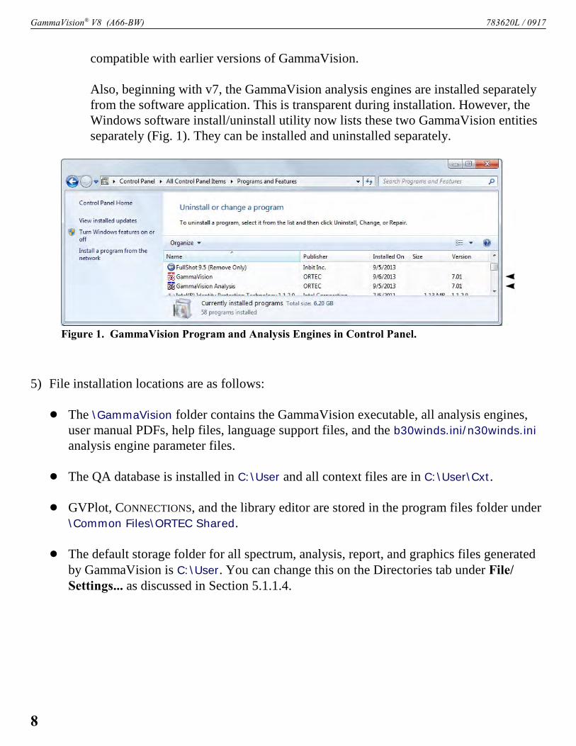
GammaVision® V8 (A66-BW) 783620L / 0917
Figure 1. GammaVision Program and Analysis Engines in Control Panel.
compatible with earlier versions of GammaVision.
Also, beginning with v7, the GammaVision analysis engines are installed separatelyfrom the software application. This is transparent during installation. However, theWindows software install/uninstall utility now lists these two GammaVision entitiesseparately (Fig. 1). They can be installed and uninstalled separately.
5) File installation locations are as follows:
! The \GammaVision folder contains the GammaVision executable, all analysis engines,user manual PDFs, help files, language support files, and the b30winds.ini/n30winds.ini
analysis engine parameter files.
! The QA database is installed in C:\User and all context files are in C:\User\Cxt.
! GVPlot, CONNECTIONS, and the library editor are stored in the program files folder under\Common Files\ORTEC Shared.
! The default storage folder for all spectrum, analysis, report, and graphics files generatedby GammaVision is C:\User. You can change this on the Directories tab under File/Settings... as discussed in Section 5.1.1.4.
8

783620L / 0917 2. INSTALLING GAMMAVISION
Figure 2. Detector Numbering and Descriptions.
2.3. Step 3: Establishing Communication WithYour ORTEC MCBs
1) If you have purchased new ORTEC spectroscopy hardware, connect it and power it onaccording to its accompanying hardware manual.5
2) Connect and power on all local and network ORTEC instruments that you wish to use, aswell as their associated computers. Otherwise, the MCB Configuration program will notdetect them during installation. Any instruments not detected can be configured at a latertime.
3) To start the software, enter the letters mcb in the “search programs and files” box at thebottom of the Windows Start menu, then click the MCB Configuration search result; oropen the Windows Start menu and click GammaVision, then MCB Configuration. TheMCB Configuration program will locate all of the powered-on ORTEC Detectors on thelocal computer and the network, and display the list of instruments found (the Master Instru-ment List; Fig. 2). If you wish, you may enter customized instrument ID numbers anddescriptions (Section 2.3.2). When you close the dialog, any changes you have made to an IDnumber or description will be written back to the corresponding Detector.
5The first time a particular MCB model is connected, a”found new hardware” wizard will start up. Choose not to“search the internet for a driver” option, then choose to automatically search for the driver.
9

GammaVision® V8 (A66-BW) 783620L / 0917
Figure 3. New Instruments Must Have a Non-Zero ID Number.
2.3.1. Configuring a New Instrument
The first time a new instrument is detected, thedialog shown in Fig. 3 will remind you that allnew instruments must be assigned a unique,non-zero ID number.6 Click OK. You caneither manually change the ID Number andDescription as described in the next subsection,or you can click the Renumber New buttonto renumber only the new instruments.
NOTE We recommend not using the Renumber All button. In addition, we strongly recom-mend not renumbering Detectors that “belong” to other users, as this could affect theinteraction between their Detectors and their ORTEC software, for instance, if theycontrol their Detectors with .JOB files (e.g., the .JOB file command SET_DETECTOR 5),or use the GammaVision or ISOTOPIC spectroscopy applications. See also the follow-ing NOTE and the NOTES in the next section.
NOTE FOR MULTIPLE USERS ON A NETWORKThere are two ways to reduce the chance that other users will renumber your Detectors:
! Add the -I flag to their MCB Configuration command line, as described in Section 2.4.2. Thiswill allow you to assign whatever ID Numbers you wish, regardless of the numbers assignedby other users on your network. (Ideally, everyone using ORTEC instruments on your networkshould make this change.)
! To prevent others from renumbering your Detectors (or performing any other actions exceptread-only viewing), password-lock your Detectors with the Lock/Unlock Detector command(Section 5.7.3). If you lock a detector that will be controlled by a JOB stream, remember toinclude the proper password-unlock commands in your .JOB file (Section 10.1.1.4).
6If this is a first-time installation of ORTEC products, all your instruments will be “new.”
10

783620L / 0917 2. INSTALLING GAMMAVISION
Figure 4. Change Detector Number or Description.
2.3.2. Customizing ID Numbers and Descriptions
If you wish, you can changethe instrument ID Numbers andDescriptions by double-clickingon an instrument entry in the Con-figure Instruments dialog. Thiswill open the Change Descriptionor ID dialog (Fig. 4). It shows thephysical Detector location (read-only), and allows you to changethe ID Number and Description.
Make the desired changes and click Close. Any changes you have made to an ID number ordescription will then be written back to the corresponding Detector.
If a modified description has already been applied to a particular instrument, you can restore thedefault description by deleting the entry in the Description field and re-running MCB Config-uration. After MCB Configuration runs, the default description will be displayed.
2.4. Caution: Running the MCB Configuration ProgramCan Affect Quality Assurance
Detector identification in GammaVision is based on the instrument ID number and descriptionassigned to a Detector by the MCB Configuration program. Instrument ID number and descrip-tion are assigned when MCB Configuration polls the local computer and network for attachedORTEC MCBs and then builds a Master Detector List of the instruments found. This instrumentidentification is then used for all QA measurements.
NOTE FOR GAMMA TOTAL USERS
The filenaming conventions for EDF’s Gamma Total effluent reports (Section 5.5.1.9) arebased on a single-digit identifier for the MCBs used for data acquisition. When first setting upGammaVision, be sure to choose instrument ID numbers that each end with a unique digit,e.g., 0–9 (for instance, 901, 22, 13, 4, 375, and so on). Note that in Fig. 2, two of the instru-ments in the list share 1 as the final digit of their ID number, and two share 4 as the final digit.To avoid having two MCBs that generate reports with the same device identification number,two of these MCBs should ideally be reassigned ID numbers with unique final digits.
11

GammaVision® V8 (A66-BW) 783620L / 0917
Figure 5. Original MCB Configuration Showing Our TwoDSPEC Pro MCBs.
Once you have established QA settings for those detectors and subsequently collected data usingthem, if you then re-run the MCB Configuration program for any reason, you must ensure eachinstrument is still assigned its previous instrument ID number and description before collectingany more data. Allowing the MCB Configuration program to assign a new instrument identi-fication to a detector, and then using that new identification, interrupts the orderly accumulationof QA records. This is because GammaVision treats the renumbered detector as new, with zero“previous QA measurements” and with potentially incorrect QA settings.
If you must re-run the MCB Configuration program, you can avoid any renumbering problemseither by not renumbering instruments or by manually editing the instrument numbers for all ofthe Detectors on the Master Detector List for your computer. Doing so requires that you keep aseparate record of the ID and Description for each MCB on your system. Note spelling, spacing,and uppercase/lowercase; these details will be necessary when recreating the Description textstring. Let us use the following example to illustrate the process:
Suppose you are using two MCBs for your GammaVision measurements and in your originalMCB Configuration you configured them as 1 DSPEC PRO 1 and 4 DSPEC PRO 4. This isdepicted in Fig. 5. The numerical prefixes 1 and 4 are the IDs and the corresponding text stringsare the Descriptions.
Suppose we add one new MCB to the system and remove two. We must then manually re-runMCB Configuration to add the new instrument to the Master Detector List. Suppose we thenfind that our two DSPEC Pro units, originally assigned IDs of 1 and 4, have been renumberedwith IDs of 2 and 3, respectively. Before closing the Configure Instruments dialog, double-
12
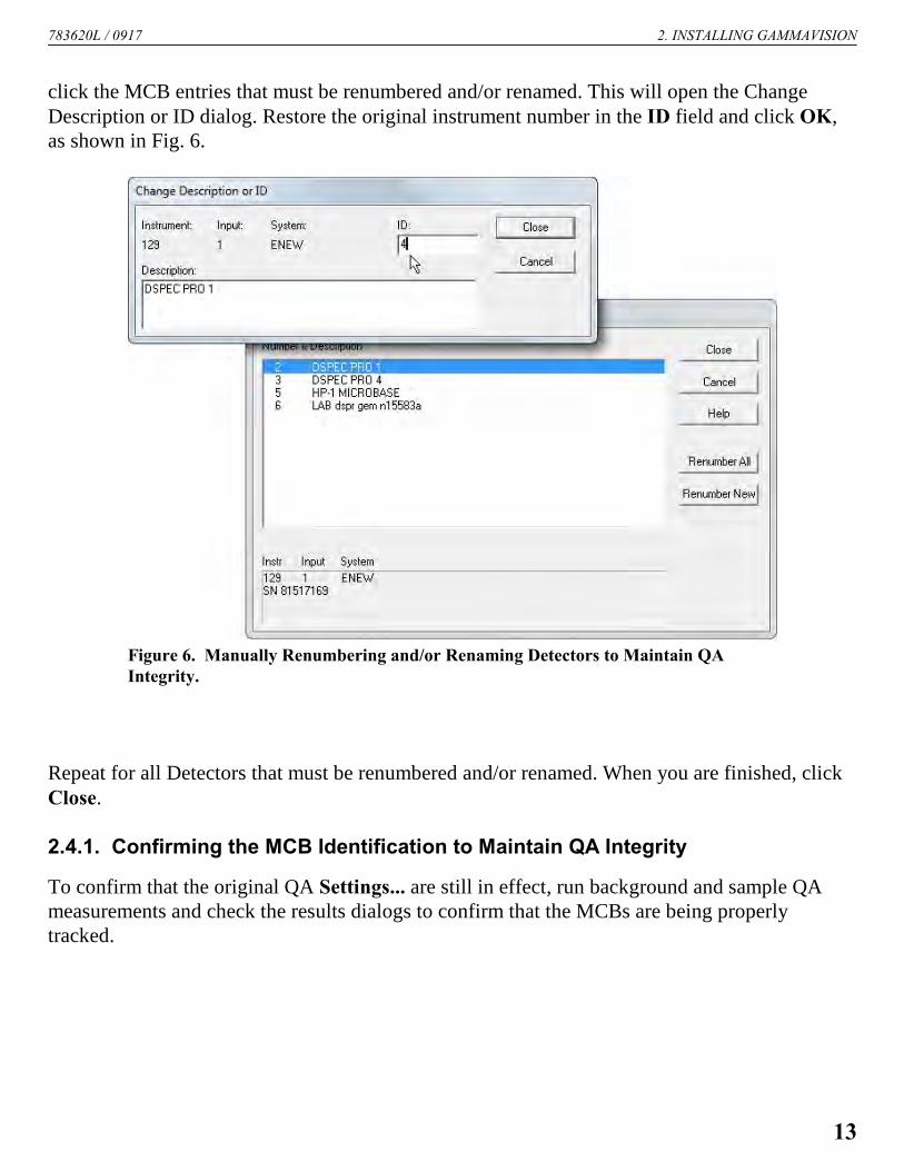
783620L / 0917 2. INSTALLING GAMMAVISION
Figure 6. Manually Renumbering and/or Renaming Detectors to Maintain QAIntegrity.
click the MCB entries that must be renumbered and/or renamed. This will open the ChangeDescription or ID dialog. Restore the original instrument number in the ID field and click OK,as shown in Fig. 6.
Repeat for all Detectors that must be renumbered and/or renamed. When you are finished, clickClose.
2.4.1. Confirming the MCB Identification to Maintain QA Integrity
To confirm that the original QA Settings... are still in effect, run background and sample QAmeasurements and check the results dialogs to confirm that the MCBs are being properlytracked.
13

GammaVision® V8 (A66-BW) 783620L / 0917
2.4.2. Editing the MCB Configuration Command Line
The command line for the MCB Configuration program is:7
“C:\Program Files\Common Files\ORTEC Shared\UMCBI\mcbcon32.exe”
You can modify the way the MCB Configuration program runs by adding one or more of thefollowing flags to the command line. You can use any combination of flags or none, and theflags are not case-sensitive.
-I Ignore duplicate IDs. MCB Configuration allows you to accept an instrument list withduplicate detector ID numbers; no renumbering is required. Useful for customers usingour QA tools, JOB commands, and “Gamma Total” function; and when sharing a net-work with other users of ORTEC MCBs.
-L Configure only local instruments (i.e., no discovery of ORTEC instruments across anetwork except “attached” digiBASE-E units). This can significantly reduce the time ittakes to run MCB Configuration, if you have only local MCBs.
-P Append all newly discovered instruments to the existing list (i.e., don’t clear the exist-ing list before starting discovery). Useful when you don’t have all your instrumentsconnected or powered-on at the same time but wish to configure new detectors.
There are two ways to modify the MCB Configuration command line:
! To retain the flags from use to use, right-click MCB Configuration in the Start menu,select Properties, then in the Target field, add the flags outside the right-hand quotationmark and click OK. For instance:
“C:\Program Files\Common Files\ORTEC Shared\UMCBI\mcbcon32.exe” -I -L
! To temporarily change the command line, open the Windows Start menu’s Run... dialog,browse to locate the MCB Configuration file, mcbcon32.exe, add the flags outside theright-hand quotation mark, and click OK.
You are now ready to register your copy of GammaVision, as discussed in the next section.
7As noted earlier, 32-bit Windows uses the \Program Files folder and 64-bit Windows uses \Program Files(x86).
14

783620L / 0917 2. INSTALLING GAMMAVISION
Figure 7. Register GammaVision.
2.5. Product Registration
GammaVision requires product registration within 60 days after installation. Until registered, thedialog shown in Fig. 7 opens each time you start the program. Click the Register Later buttonto bypass registration and access the full-featured GammaVision application. Once you enter theregistration key and click Register Now, this dialog will no longer be displayed. After 60 daysof unregistered use, the Register Later option will be disabled and GammaVision will shutdown when you close this dialog.
To obtain your registration key and activate your copy of GammaVision, you may call theORTEC telephone extension listed on the GammaVision Registration dialog. You will need theserial number for your copy of the software (located on the box). Enter the registration key onthe GammaVision Registration dialog and click Register Now.
Alternatively, you may fill out and submit the registration form as follows:
1) Click Generate ORTEC Registration Form to open the ORTEC Registration Form dialogshown in Fig. 8.
2) If any paper manuals are available for this release, they will be listed on the dialog. If you donot wish to order paper manuals, simply enter the Serial Number for your copy of Gamma-Vision. The number is located on the box. No other information is required for registration.Skip to step 4.
15

GammaVision® V8 (A66-BW) 783620L / 0917
Figure 8. Create a Registration File.
3) To order paper manuals, enter the Serial Number for the software, then mark the desiredcheckbox(es) and complete all of the surface mailing address fields marked with (*).
4) Click the Write ORTEC Registration File button to create a text file containing your regis-tration information. A standard file-save dialog will open. Enter a filename and location, andclick Save. Email this file to the ORTEC address listed on the GammaVision Registrationdialog. We will respond promptly with your registration key.
5) Enter the registration key on the GammaVision Registration dialog and click Register Now.
2.6. Enabling Additional ORTEC Device Drivers andAdding New MCBs
You can enable other device drivers later with the Windows Add/Remove Programs utility onthe Control Panel. Follow the instructions in the CONNECTIONS Driver Update Kit.
16

3. GETTING STARTED — A GAMMAVISIONTUTORIAL
3.1. Introduction
This chapter provides a series of straightforward examples to help you become familiar withGammaVision’s basic operations and move on quickly to full use. We will cover the followingbasic functions:
! Recalling a spectrum file from disk! Performing a simple analysis of the spectrum! Loading a nuclide library! Using the library editor! Energy calibration! Efficiency calibration! The calibration wizard! Getting a Detector ready for data acquisition
To display help for any of the dialogs, put the mouse pointer on the item and click the rightmouse button to display the button. Now click the left mouse button to display thehelp message. After reading the help message, click the left mouse button to close the messagebox.
To make the discussion easier and more realistic, the optionally installed sample files in C:\User
\GammaVision V8 Examples will be used in the remainder of the chapter.8 You may either leavethem in the examples folder or copy them to C:\User.
GVDEMO.SPC GVDEMO.EFTGVDEMO.LIB GVDEMO.ENT
Before we actually begin, here is a short note on the Detector and buffer concept used inGammaVision.
A spectrum can exist in three places in GammaVision:
! In an MCB (which we call a Detector)! In computer memory (a buffer window in GammaVision)! In a file on disk
8If you chose not to install the example files, you may wish to reinstall GammaVision and choose to install thefiles.
17

GammaVision® V8 (A66-BW) 783620L / 0917
Figure 9. GammaVisionMenu.
The Detector is where the data are gathered from the HPGe detector. Data can be displayed andmanipulated directly in the Detector memory or in a buffer window. They can be copied from theDetector to either the buffer or disk. Data can also be copied from disk to the buffer. Copyingdata will overwrite the existing buffer contents. A warning message is displayed before any dataare overwritten and lost. Actions on the data in the buffer have no effect on data acquisitiontaking place in a Detector — GammaVision maintains separate calibrations and viewing settingsfor each Detector and buffer window.
GammaVision’s multi-detector interface allows you to open up to eight Detector windows andeight buffer windows at a time. If you try to open a ninth window, the program will ask if youwish to close the oldest window. If you answer Yes, the oldest window will close and the newDetector or buffer window will open. To cancel and keep that oldest window open, click No.
In addition, the Acquisition Settings dialog (Acquire/Acquisition Settings...) now gives you thechoice of starting all displayed Detectors simultaneously (All MCBs) or one Detector at a time(Current MCB); or Prompts you to either start all MCBs or start only the current MCB.
3.2. Starting GammaVision
To start GammaVision, enter gamm in the “search pro-grams and files” box on the Windows Start panel, thenclick the GammaVision search result; or open the Win-dows Start menu and click GammaVision, and Gamma-Vision (Fig. 9). You can also start GammaVision by enter-ing run in the search box and choosing the Run option;or (in XP) by selecting Run from the Start menu. The Runoption allows you to start up from the command line, withor without arguments, as described in Section A.1.
If you have not yet entered the Registration Key for yourcopy of GammaVision, the registration dialog will open,as discussed in Section 2.5. You may either enter the Regis-tration Key (after which the registration dialog will not bedisplayed again); or, for 60 days after installation, youmay bypass registration by clicking on Register Later.
GammaVision will check for Detectors, then display a screen similar to Fig. 10.
18

783620L / 0917 3. GETTING STARTED — A GAMMAVISION TUTORIAL
Figure 10. Example GammaVision Opening Screen.
Figure 11. Recalling a Spectrum File.
3.2.1. Recalling a Spectrum
If a Detector or buffer window is alreadyopen, click its Close box ( ). Next,recall GVDEMO.SPC from the the menubar by clicking on File, then Recall....This will open a dialog showing the listof spectrum files in the C:\User folder.If you did not copy the example filesinto this folder, look in the \Gamma-
Vision V8 Examples folder, as shownin Fig. 11. From the list of files, double-click GVDEMO.SPC, or click onceon the file name and then Open.
A buffer window will open, displayingGVDEMO.SPC (Fig. 12). The Status Side-bar on the right of the screen will nowshow details about this spectrum.
19

GammaVision® V8 (A66-BW) 783620L / 0917
Figure 12. Calibrated Spectrum Recalled from Disk File.
Note the vertical marker line, which you can move by left-clicking the mouse on a different partof the spectrum. The marker information line at the bottom of the display reflects the channelcontents at the marker’s location. You can tell that this spectrum is already calibrated becausethe information about the marker reads in units of energy, keV. (An uncalibrated spectrumwould instead display the word uncal.)
3.2.2. The Simplest Way To Do An Analysis
Select a portion of the GVDEMO.SPC spectrum for analysis by positioning the mouse on or nearthe 122 keV peak in the Full Spectrum View (Fig. 13), which will be located near the left edgeof the window, and clicking the left mouse button. This will move the marker to the mousepointer. The Expanded Spectrum View will now show this part of the spectrum.
20

783620L / 0917 3. GETTING STARTED — A GAMMAVISION TUTORIAL
Figure 13. Full Spectrum Window.
Figure 14. Analyze/Interactivein Viewed Area.
Now expand this part of the spectrum by clicking on the Zoom In button ( ) on the toolbar
one or more times. As you zoom in, the Full Spectrum View will show which portion of thespectrum is expanded, and the Expanded Spectrum View will display this part of the spectrum(see Fig. 12). If the 122 keV region is not on the screen, point the mouse in the Full SpectrumView and try again.
On the menu bar, click Analyze, and select Interactive in viewed area... (see Fig. 14). Gamma-Vision will automatically analyze the selected region and display the results. The Analysis Side-bar will open, superimposed on the Status Sidebar, the peak fit(s) will be shown graphically, andthe numerical results will be displayed in an Analysis Results Table window, as shown inFig. 15.
That’s all it takes to do an analysis!
There are several functions that you can access at this point, but first we will load a workingnuclide library and check some parameters. Exit this analysis session by clicking on theAnalysis Sidebar’s Close button ( ). This will close the Analysis Sidebar and the tablewindow.
21

GammaVision® V8 (A66-BW) 783620L / 0917
Figure 15. Completed Analysis, Showing Results Table and Analysis Sidebar.
Figure 16. Load aLibrary fromMenu.
3.2.3. Loading a Library
From the menu bar, select Library, then Select File... as shownin Fig. 16. This will open a list of nuclide libraries in the currentdirectory.
Select the library file GVDEMO.LIB and click OK to load it. Thefollowing message will appear on the Supplemental InformationLine at the bottom of the GammaVision window:
GVDEMO.LIB: 1024 Bytes; 9 Nuclides /9 alloc.; 16 Peaks /16 alloc.
This message describes the library just loaded. GVDEMO.LIB is 1024 bytes in size, has 9 nuclideswith space for 9, and has 16 peaks with space for 16.
22
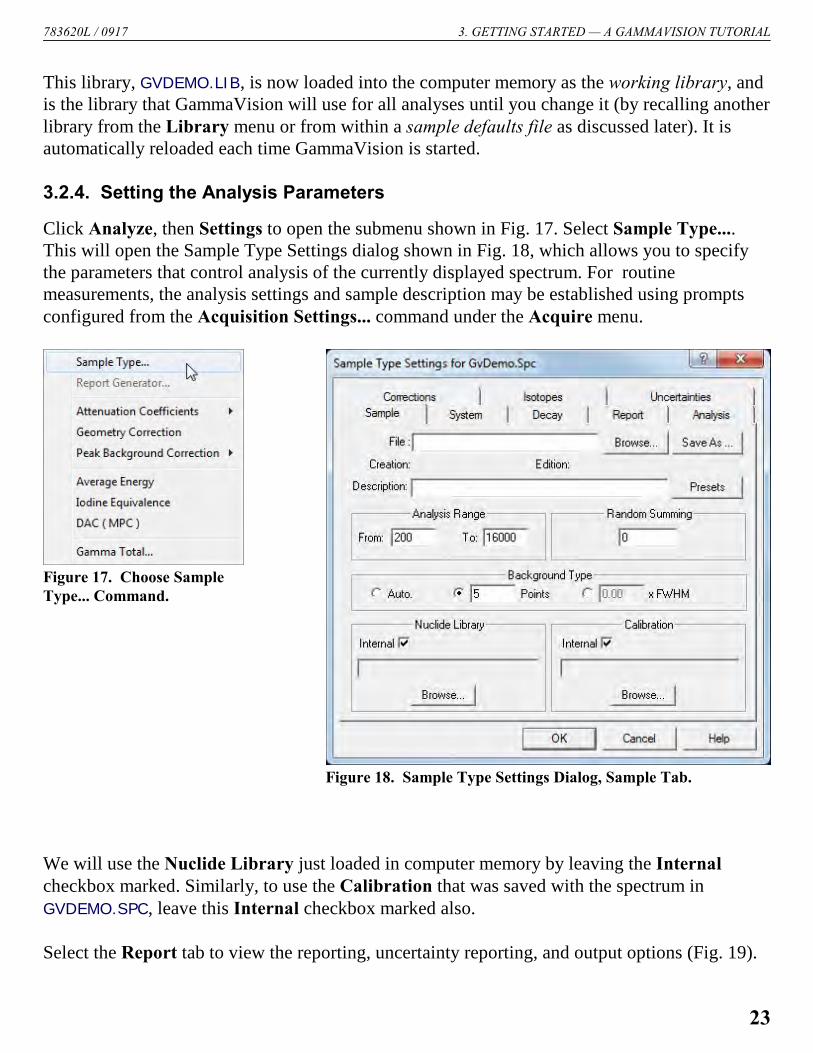
783620L / 0917 3. GETTING STARTED — A GAMMAVISION TUTORIAL
Figure 17. Choose SampleType... Command.
Figure 18. Sample Type Settings Dialog, Sample Tab.
This library, GVDEMO.LIB, is now loaded into the computer memory as the working library, andis the library that GammaVision will use for all analyses until you change it (by recalling anotherlibrary from the Library menu or from within a sample defaults file as discussed later). It isautomatically reloaded each time GammaVision is started.
3.2.4. Setting the Analysis Parameters
Click Analyze, then Settings to open the submenu shown in Fig. 17. Select Sample Type....This will open the Sample Type Settings dialog shown in Fig. 18, which allows you to specifythe parameters that control analysis of the currently displayed spectrum. For routinemeasurements, the analysis settings and sample description may be established using promptsconfigured from the Acquisition Settings... command under the Acquire menu.
We will use the Nuclide Library just loaded in computer memory by leaving the Internalcheckbox marked. Similarly, to use the Calibration that was saved with the spectrum inGVDEMO.SPC, leave this Internal checkbox marked also.
Select the Report tab to view the reporting, uncertainty reporting, and output options (Fig. 19).
23

GammaVision® V8 (A66-BW) 783620L / 0917
Figure 19. Report Tab.
Mark all of the Reporting Options except ISO NORM, and make sure the Total option isselected in the Uncertainty Reporting section.
To send the output to a printer, go to the Output section of the screen and click the Printerradio button to mark it with a dot.
To send the output to a file instead, click the File radio button, and leave the asterisk ( * ) as thefilename. Leaving the asterisk ensures that the report file will have the same filename as thespectrum (however, it will have the extension .RPT). You can, however, enter a path and file-name in this field to force the report to be saved to the filename you specify.
To send the output to a text processing program, such as Windows Notepad (which is thedefault), click the Program radio button.
Click all four checkboxes in the Reporting Options section of the screen, then click OK.
Select Analyze and Entire spectrum in memory.... Spectra can be analyzed in the buffer (as wehave done here), directly from disk, or in the Detector memory (when the Detector is not count-
24
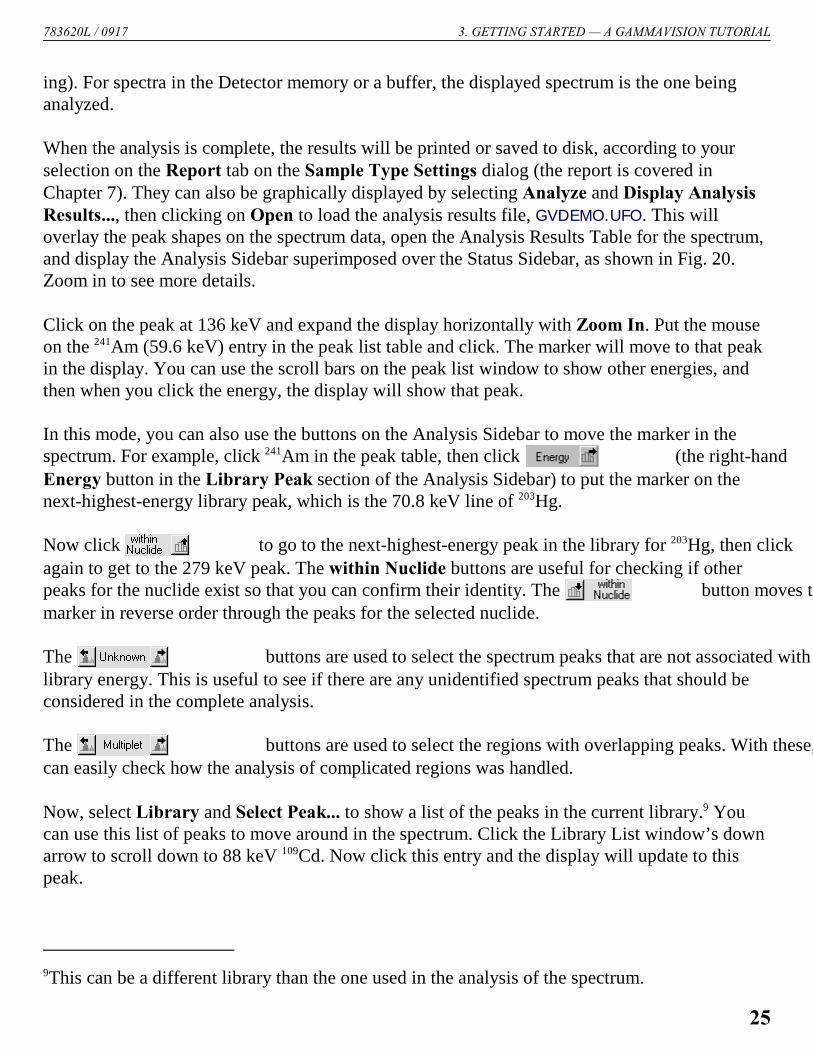
783620L / 0917 3. GETTING STARTED — A GAMMAVISION TUTORIAL
ing). For spectra in the Detector memory or a buffer, the displayed spectrum is the one beinganalyzed.
When the analysis is complete, the results will be printed or saved to disk, according to yourselection on the Report tab on the Sample Type Settings dialog (the report is covered inChapter 7). They can also be graphically displayed by selecting Analyze and Display AnalysisResults..., then clicking on Open to load the analysis results file, GVDEMO.UFO. This willoverlay the peak shapes on the spectrum data, open the Analysis Results Table for the spectrum,and display the Analysis Sidebar superimposed over the Status Sidebar, as shown in Fig. 20.Zoom in to see more details.
Click on the peak at 136 keV and expand the display horizontally with Zoom In. Put the mouseon the 241Am (59.6 keV) entry in the peak list table and click. The marker will move to that peakin the display. You can use the scroll bars on the peak list window to show other energies, andthen when you click the energy, the display will show that peak.
In this mode, you can also use the buttons on the Analysis Sidebar to move the marker in thespectrum. For example, click 241Am in the peak table, then click (the right-handEnergy button in the Library Peak section of the Analysis Sidebar) to put the marker on thenext-highest-energy library peak, which is the 70.8 keV line of 203Hg.
Now click to go to the next-highest-energy peak in the library for 203Hg, then click
again to get to the 279 keV peak. The within Nuclide buttons are useful for checking if otherpeaks for the nuclide exist so that you can confirm their identity. The button moves themarker in reverse order through the peaks for the selected nuclide.
The buttons are used to select the spectrum peaks that are not associated with alibrary energy. This is useful to see if there are any unidentified spectrum peaks that should beconsidered in the complete analysis.
The buttons are used to select the regions with overlapping peaks. With these, youcan easily check how the analysis of complicated regions was handled.
Now, select Library and Select Peak... to show a list of the peaks in the current library.9 Youcan use this list of peaks to move around in the spectrum. Click the Library List window’s downarrow to scroll down to 88 keV 109Cd. Now click this entry and the display will update to thispeak.
9This can be a different library than the one used in the analysis of the spectrum.
25
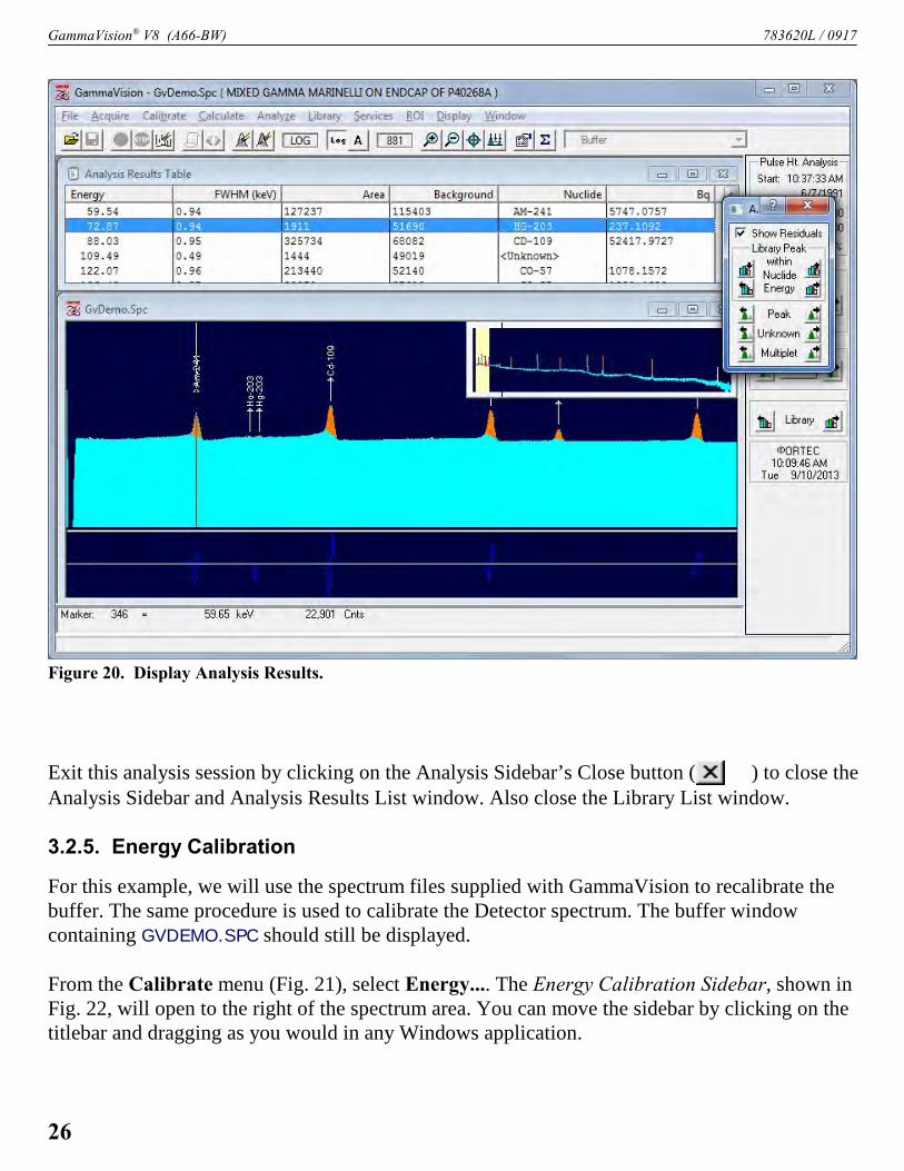
GammaVision® V8 (A66-BW) 783620L / 0917
Figure 20. Display Analysis Results.
Exit this analysis session by clicking on the Analysis Sidebar’s Close button ( ) to close theAnalysis Sidebar and Analysis Results List window. Also close the Library List window.
3.2.5. Energy Calibration
For this example, we will use the spectrum files supplied with GammaVision to recalibrate thebuffer. The same procedure is used to calibrate the Detector spectrum. The buffer windowcontaining GVDEMO.SPC should still be displayed.
From the Calibrate menu (Fig. 21), select Energy.... The Energy Calibration Sidebar, shown inFig. 22, will open to the right of the spectrum area. You can move the sidebar by clicking on thetitlebar and dragging as you would in any Windows application.
26

783620L / 0917 3. GETTING STARTED — A GAMMAVISION TUTORIAL
Figure 21. StartEnergy Calibrationfrom Menu. Figure 22. Energy Calibration Sidebar.
Figure 23. EnergyCalibration SidebarControl Menu.
This time, so that we start from the very beginning, clear thecurrent energy calibration by clicking on the icon to the left ofthe “Energy Calibration” title. This will open the control menushown in Fig. 23. Click on Destroy. The Marker InformationLine now shows the legend uncal.
Move the cursor to channel 8226, the location of the upper 60Copeak, at 1332.5 keV. Do this directly in the full window or byusing the buttons until you get there. Click once in
the E= field at the top of the Energy Calibration Sidebar, enterthe correct energy for this peak (1332.5 keV), and click Enter.The system will automatically perform a simple calibration basedon this peak and the assumption that channel zero is energy zero.The graphs of the calibration and the table of values will beshown on the display, as in Fig. 24.
If the screen becomes too visually crowded, you can either move one or more windows untilthey are nearly “stacked” atop each other (leave at least an edge or corner of each window show-ing); or close one or more windows by clicking on their Close box ( ). However, do not closethe Energy Calibration Sidebar or you’ll end the calibration session. Rearrange and/or resize thewindows as needed.
Now we can use the library; click Library/Select Peak to reopen the Library List window.Double-click the 122.07 keV peak of 57Co in the library list. The marker will move close to, butnot precisely on, that peak in the spectrum based on our current “one-point calibration.”
27

GammaVision® V8 (A66-BW) 783620L / 0917
Figure 24. Energy Calibration Display.
Use the buttons to put the cursor on the peak, then click once on the 122 keV entry
in the library list. Note that the E= 122.07 keV in the Energy Calibration Sidebar already has theappropriate energy from the library, and you need only accept it by clicking on Enter. Therefitted calibration curve is automatically displayed.
Proceed through the library list in Table 1 adding the peaks (in any order) into the calibration.To do this, double-click within 2 channels of the peak center, then click Enter.
If you decide that you don’t want one of the peaks, you can delete it at will by clicking on theDelete Energy button on the Calibration Sidebar.
Now examine the Energy Table and note that the Deltas (the differences between data pointsand the fit to the data points) are small. Next, bring the Energy plot window to the front and
28

783620L / 0917 3. GETTING STARTED — A GAMMAVISION TUTORIAL
Nuclide Energy (keV)88Y 1836.01
57Co 122.0760Co 1173.260Co 1332.5188Y 898.02
137Cs 661.66113Sn 391.69203Hg 279.17109Cd 88.03
241Am 59.54
Table 1. Source Energies.
Figure 25. FWHM Fit Selection.
visually inspect the calibration curve, resizing the windows as needed to allow a closer examin-ation of the graphical fit.
Click the FWHM (full width at half maximum) radio button on the lower section of the Calibra-tion Sidebar to display the table of FWHM results and the FWHM graph (which is shown inFig. 25). The FWHM fit uses the peaks specified in the energy fit. If FWHM of any peak has adeviation of more than 25% between the actual and fitted values, a warning message isdisplayed.
Save the energy table for later use: click the Calibration Sidebar’s Save button, enter a namesuch as GVDEMO for the table filename, and click Save. GammaVision willappend the extension .ENT to the filename.
To examine the Energy Table, open the Calibration Sidebar’s control menu and select Edit File.This table is a list of peak energies and the associated channel and FWHM values used for thecalibration.
The energy calibration is complete; we shall consider this to be a “good” energy calibration forthe purposes of this demonstration. Close the calibration session by selecting the system menu inthe calibration and selecting the Close option. This new energy calibration is now held inmemory but is not yet stored on disk.
29

GammaVision® V8 (A66-BW) 783620L / 0917
Figure 26. Efficiency Calibration Sidebar.
3.2.5.1. Auto Calibration
The Auto Calibrate button is the fastest and easiest way to do the energy calibration. Just clickAuto Calibrate to use the working library to calibrate the displayed spectrum with no otherinputs. The current calibration is erased before the new calibration is started.
Select Close from the sidebar’s control menu.
3.2.6. Efficiency Calibration
Select Calibrate from the menu bar, thenEfficiency. This opens the Efficiency Cali-bration Sidebar, shown in Fig. 26 (note itssimilarity to the Energy Calibration Sidebar).
We want to start from the beginning of theprocess, so open the sidebar’s control menu(click the icon on the left of the title bar)and select Destroy.
The Library List window should be visible,but if not, click Library/Select Peak... toreopen it.
From the library, double-click the 1332.5 keV peak of 60Co. The marker will move to the cor-responding peak and GammaVision will enter the energy in the top section of the EfficiencyCalibration Sidebar.
In the upper section of the sidebar, click the Calc... button to open the Efficiency CalculationWorksheet (Fig. 27).
Enter the date and the time from the calibration certificate (see Table 2), as Oct-01-90 12:00.Enter the gammas per second (5838) from the calibration certificate for 60Co at 1332.5 keV.Select GPS from the units droplist. Note that the from Library box is checked; this shows thatthe half-life came from the library.
At this point, the Calculate Efficiency= button at the top of the worksheet should be active(black rather than gray). If it is disabled (gray), one or more of the data inputs is either incorrector has not been entered. When you have completed all fields and Calculate Efficiency= isactivated, click it to obtain the efficiency value at this energy. Click OK to insert the value in theefficiency table. You will see that the value appears in the Efficiency Table window.
30
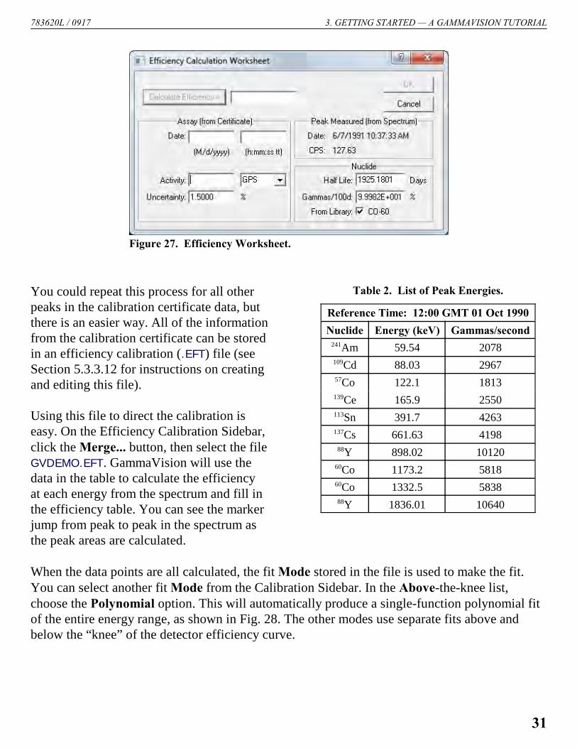
783620L / 0917 3. GETTING STARTED — A GAMMAVISION TUTORIAL
Figure 27. Efficiency Worksheet.
Reference Time: 12:00 GMT 01 Oct 1990
Nuclide Energy (keV) Gammas/second241Am 59.54 2078109Cd 88.03 296757Co 122.1 1813139Ce 165.9 2550113Sn 391.7 4263137Cs 661.63 4198
88Y 898.02 1012060Co 1173.2 581860Co 1332.5 583888Y 1836.01 10640
Table 2. List of Peak Energies.You could repeat this process for all otherpeaks in the calibration certificate data, butthere is an easier way. All of the informationfrom the calibration certificate can be storedin an efficiency calibration (.EFT) file (seeSection 5.3.3.12 for instructions on creatingand editing this file).
Using this file to direct the calibration iseasy. On the Efficiency Calibration Sidebar,click the Merge... button, then select the fileGVDEMO.EFT. GammaVision will use thedata in the table to calculate the efficiencyat each energy from the spectrum and fill inthe efficiency table. You can see the markerjump from peak to peak in the spectrum asthe peak areas are calculated.
When the data points are all calculated, the fit Mode stored in the file is used to make the fit.You can select another fit Mode from the Calibration Sidebar. In the Above-the-knee list,choose the Polynomial option. This will automatically produce a single-function polynomial fitof the entire energy range, as shown in Fig. 28. The other modes use separate fits above andbelow the “knee” of the detector efficiency curve.
31

GammaVision® V8 (A66-BW) 783620L / 0917
Figure 28. Polynomial Efficiency Fit.
Figure 29. ControlMenu.
The fit will take place automatically. You can then view it bybringing the Efficiency calibration fit window forward. Click thewindow’s control menu to choose scaling and grid display options(see Fig. 29). The marker line in the efficiency graph window willbe at the energy of the peak selected in the Library List or theEfficiency Table window.
We will accept this calibration and close the calibration sessionby clicking the Calibration Sidebar’s Close button. Now save thiscalibration to disk by selecting Calibrate and Save Calibration....Give the calibration file the name GVDEMO. GammaVision willattach the default .CLB extension to the filename.
32
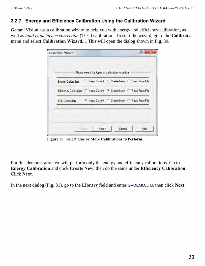
783620L / 0917 3. GETTING STARTED — A GAMMAVISION TUTORIAL
Figure 30. Select One or More Calibrations to Perform.
3.2.7. Energy and Efficiency Calibration Using the Calibration Wizard
GammaVision has a calibration wizard to help you with energy and efficiency calibration, aswell as total coincidence correction (TCC) calibration. To start the wizard, go to the Calibratemenu and select Calibration Wizard.... This will open the dialog shown in Fig. 30.
For this demonstration we will perform only the energy and efficiency calibrations. Go toEnergy Calibration and click Create New, then do the same under Efficiency Calibration.Click Next.
In the next dialog (Fig. 31), go to the Library field and enter GVDEMO.LIB, then click Next.
33

GammaVision® V8 (A66-BW) 783620L / 0917
Figure 31. Enter the Library File to be Used in the EnergyCalibration.
Figure 32. Enter the Certificate File to be Used in theEfficiency Calibration.
On the third wizard screen (Fig. 32), enter GVDEMO.EFT as the Certificate File to be used in theefficiency calibration.
34

783620L / 0917 3. GETTING STARTED — A GAMMAVISION TUTORIAL
Figure 33. Energy and Efficiency Calibration Results.
Now click Next. GammaVision will now perform the two calibrations. The results are shown inFig. 33. The Fit vs. Energy display on the lower right refers to the true-coincidence correctioncalibration. Since this example does not use the TCC calibration, its display is markedUncalibrated.
Click Save Calibration and assign the filename GVDEMO.CLB. Finally, click Finish — that’sall there is to it!
3.2.8. Changing a Library
Select Library/Edit/GammaVision Editor... from the menu bar. This will open the Editingdialog (Fig. 34), which allows you to change, add, or delete nuclide and gamma-ray values in thecurrently loaded nuclide library file.
Select the nuclide 60Co from the left-hand section of the dialog. All the gamma-ray energies orpeaks for this nuclide will then appear in the Peaks section; select the 1332.5 keV peak. ClickEdit... in the Peaks section. This will open the Edit Library Peak dialog (Fig. 35), which willshow the current values and allow you to change the energy and gammas-per-disintegration ofthe 1332.5 keV line.
Click the Gammas per 100 disintegrations field and change the value, then click OK. You willsee that the Gammas per 100 Disintegrations value for this peak has been changed to thenumber you just entered.
35
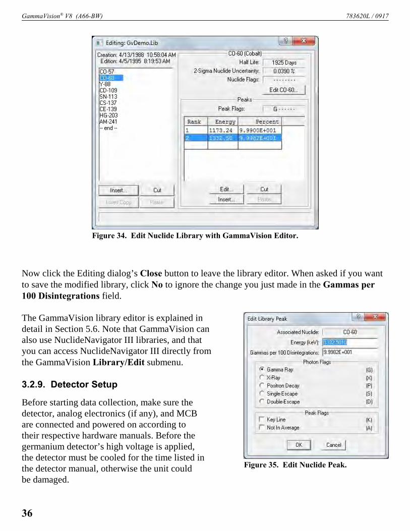
GammaVision® V8 (A66-BW) 783620L / 0917
Figure 34. Edit Nuclide Library with GammaVision Editor.
Figure 35. Edit Nuclide Peak.
Now click the Editing dialog’s Close button to leave the library editor. When asked if you wantto save the modified library, click No to ignore the change you just made in the Gammas per100 Disintegrations field.
The GammaVision library editor is explained indetail in Section 5.6. Note that GammaVision canalso use NuclideNavigator III libraries, and thatyou can access NuclideNavigator III directly fromthe GammaVision Library/Edit submenu.
3.2.9. Detector Setup
Before starting data collection, make sure thedetector, analog electronics (if any), and MCBare connected and powered on according totheir respective hardware manuals. Before thegermanium detector’s high voltage is applied,the detector must be cooled for the time listed inthe detector manual, otherwise the unit couldbe damaged.
36

783620L / 0917 3. GETTING STARTED — A GAMMAVISION TUTORIAL
Figure 36. Acquire Menu.
Figure 37. Setting the DSPEC-50 Conversion Gain.
The GammaVision installation program will have already located the Detectors available to thiscomputer. Click the Detector pick list on the right of the toolbar and select a Detector. Thespectrum displays will update to show the data in this Detector.
In the simplest mode of operation, data acquisition isstarted from the toolbar; simply click the Start button.You can use the Acquire menu (Fig. 36) to check theanalysis settings while data is being gathered. Afteracquisition stops, the analysis can proceed.
All of GammaVision’s hardware setup controls are nowin one, MCB-specific dialog. Depending on your Detector,this might include controls for conversion gain, amplifier,high voltage, shaping, data acquisition presets, and more.To access this dialog, click Acquire/MCB Properties...,or right-click the mouse anywhere in the spectrum windowto open its menu and select MCB Properties.
Some of the Detector’s internal parameters can only bechanged when the Detector is not acquiring data. To seeif the Detector is in acquisition mode, open the Acquire menu look at the menu items. If Stop isblack and Start is gray (see Fig. 36), the Detector is in acquisition mode (even if no counts areaccumulating in the MCB at the moment). If this is the case, select Stop from the menu ortoolbar.
3.2.9.1. Conversion Gain
If you wish to change the conver-sion gain, click Acquire/MCBProperties..., select the ADC tab(Fig. 37), then change the Conver-sion Gain field. The ADC gain isstored in the MCB and automaticallyrecalled from the MCB the next timeyou restart GammaVision. Notethat in this example, we are using aDSPEC-50, and that the Propertiesdialog automatically displays onlydata fields that are applicable to thisMCB.
37

GammaVision® V8 (A66-BW) 783620L / 0917
Figure 38. Monitoring the DSPEC-50 Bias Setting on theHigh Voltage Tab.
If you have software-controlled hardware (as distinguished from NIM units with front- and rear-panel hardware adjustment controls), skip to Section 3.2.9.3.
3.2.9.2. Detectors Set Up Manually
Adjust the spectroscopy amplifier gain, shaping time, and pole zero. This is a manual operationwhich should be carried out according to the instructions given in the amplifier manual. Asource with only one or two lines (e.g., 137Cs or 60Co) should be used for the initial test spectrumso you’ll be able to easily see the correct pattern of the peaks. The amplifier gain should beadjusted to align known energy peaks to the respective channel based on the energy range ofinterest. For example, if the energy range of interest is up to 2 MeV at 4000 channels, then theCo-60 1332.5 kev peak would be centered on channel 2665. With a 2 MeV range at 8000channels the 1332.5 kev peak would be centered on channel 5330.
3.2.9.3. Computer-Controlled Hardware Setup
In this section, we will use Gamma-Vision to enable the DSPEC-50'shigh voltage and adjust the spectro-scopy amplifier gain and shapingconstants.
Click Acquire/MCB Properties...to open the Properties dialog forthis MCB, and click the HighVoltage tab (see Fig. 38). Set theTarget bias. When the value ofthe detector bias matches thatshown on the detector’s QualityAssurance data sheet (also givenon the endcap label), click theOn button and note the Actualvoltage readout. If the On/Off indi-cator reads Shutdown, the detector is most likely warm. (The detector might require 3–6 hoursafter filling before it is cold enough to take bias.)
3.2.9.4. Amplifier Settings
The Amplifier tab (Fig. 39) lets you set the amplifier shaping time to either Long or Short. TheLong shaping time is the recommended choice for low to moderate count rates. The value of theshaping time (in ìs) is given in the hardware manual.
38

783620L / 0917 3. GETTING STARTED — A GAMMAVISION TUTORIAL
Figure 39. The DSPEC-50 Amplifier Tab.
Figure 40. Dead Time.
If you have a transistor-resetpreamplifier (Plus Series), selectit from the Preamplifier Typedroplist.
Click Close to apply the newMCB hardware settings.
Automatic Optimization
Select Acquire, then Start,to start the Detector counting.Next, position a source suchas 60Co such that the detector’sinput count rate (1) satisfiesthe count rate guidance instruc-tions on the bottom-left corner of the Amplifier tab or (2) is ~5000 CPS. During data collection,the Dead time will be displayed at the top of the Status Sidebar to the right of the spectrumwindow (Fig. 40).
Return to Acquire/MCB Properties... and click the Amplifier tab.Go to the Optimize section of the dialog and click Start Auto. Thiswill tell the Detector to automatically adjust the amplifier’s shapingconstants. While optimization is in progress, you will hear a periodicbeep and see the message “Optimize in progress....” This processtypically takes about 5 minutes. Remember that if you change theshaping time, you must pole zero the Detector again.
Click Close to apply the new MCB hardware settings.
Adjusting Amplifier Gain
Adjust the amplifier gain to achieve the desired energy range across the Detector display. Asource with only one or two lines (e.g., 137Cs or 60Co) should be used for the initial setup toeasily identify the applicable peaks. Figure 41 shows the 1332.5 kev peak centered on channel7348 for an energy range of approximately 2.9 MeV at channel 16000.
39

GammaVision® V8 (A66-BW) 783620L / 0917
Figure 41. Spectrum with 60Co.
To set the gain for the DSPEC-50 (and all other software-controlled ORTEC MCBs):
1) Start data collection by clicking on the Start toolbar button or by selecting Acquire/Startfrom the menu bar.
2) Select Acquire/MCB Properties... and click the Amplifier tab (Fig. 39).
3) Select the Coarse Gain setting from the droplist (if present), then move the slider to the finegain desired. The spectrum display updates continuously, even while the Properties dialog isopen.
4) Once the gain is approximately correct, click Close to close the control dialog, then use<Alt + +> and <Alt + -> to make fine gain adjustments until the peak is in the desired chan-nel. To make coarser gain adjustments, use <Alt + Shift + +> and <Alt + Shift + ->. (Thesekeyboard commands are discussed in Chapter 9.)
40

783620L / 0917 3. GETTING STARTED — A GAMMAVISION TUTORIAL
GammaVision will retain all of these settings and adjustments on exit, and will reload them fromthe MCB on restart.
*** You are now ready to acquire spectral data, calibrate, andanalyze your own sample data. ***
41

GammaVision® V8 (A66-BW) 783620L / 0917
[Intentionally blank]
42

Figure 42. GammaVisionMenu.
4. DISPLAY FEATURES
This chapter describes how to start GammaVision, explains its display features, discusses therole of the mouse and keyboard, covers the use of the toolbar and sidebars, and shows how touse additional features such as Help.
4.1. Startup
To start GammaVision, open the Windows Start menu and clickGammaVision folder, then the GammaVision icon (Fig. 42).You can also start GammaVision using the Run option from theStart menu or by creating Windows shortcuts to GammaVision inorder to use the command line option, with or without argu-ments, as described in Section A.1.
Figure 43 shows GammaVision’s principal screen features.
1) Title bar, showing the program name and the sourceof the currently active spectrum window. There is alsoa title bar on each of the spectrum windows showing thesource of the data: either the Detector name or the word“Buffer” with the spectrum name. On the far right are thestandard Windows Minimize, Maximize, and Close buttons.
2) Menu Bar, showing the available menu commands (which can be selected with either themouse or keyboard); these functions are discussed in detail in Chapter 5.
3) Toolbar, beneath the menu bar, containing icons for recalling spectra, saving them to disk,starting and stopping data acquisition, adjusting the vertical and horizontal scale of theactive spectrum window, and accessing the analysis parameters.
4) Detector List, on the toolbar, displaying the currently selected Detector (or the buffer).Clicking on this field opens a list of all Detectors currently on the computer’s GammaVisionDetector pick list, from which you can open Detector and/or buffer windows. When youselect the buffer or a Detector from the list, a new spectrum window opens, to a limit ofeight Detectors and eight buffers. (If a Detector is already displayed, selecting it from thelist does not open a duplicate window for that instrument.) If you select a Detector, the spec-trum in its memory (if any) is displayed. The droplist shows the name of the most recentlyselected Detector or buffer.
43

GammaVision® V8 (A66-BW) 783620L / 0917
Figure 43. Main GammaVision Screen Features.
5) ROI Status Area, on the right side of the menu bar, indicates whether the ROI markingmode is currently Mark or UnMark. This operates in conjunction with the ROI menucommands and arrow keys (see Section 5.8).
6) Spectrum Area, which displays multiple spectrum windows — up to eight Detector win-dows and eight buffer windows simultaneously. When you attempt to open a ninth spectrumor buffer window, GammaVision will ask if you wish to close the oldest window of thattype. Alternatively, you can turn off the Multiple Windows feature and run in the originalone-window-at-a-time mode.
Spectrum windows can be moved, sized, minimized, maximized, and closed with the mouse,as well as tiled horizontally or vertically from the Window menu. When more than one win-dow is open, only one is active — available for data manipulation and analysis — at a time.The title bar on the active window will normally be a brighter color than those on theinactive windows (the color scheme will depend on the desktop colors you have selected in
44

783620L / 0917 4. DISPLAY FEATURES
Figure 44. Full Spectrum View with ExpandedSpectrum View Area Highlighted.
Windows Control Panel). Detector windows or buffer windows containing a spectrum froman MCB will display the Detector name on the title bar. If you have opened a spectrum fileinto a buffer window, the title bar will display the filename. To switch windows, click thewindow you wish to activate, use the Window menu (see Section 5.10), or cycle betweenwindows by pressing <Ctrl + Tab>.
Each spectrum window contains an Expanded Spectrum View and a Full Spectrum View(see items 7 and 8 below).
7) The Expanded Spectrum View shows all or part of the full histogram; this allows you tozoom in on a particular part of the spectrum and see it in more detail. You can change theexpanded view vertical and horizontal scaling, and perform a number of analytical opera-tions such as peak information, marking ROIs, or calibrating the spectrum. This windowcontains a vertical line called a marker that highlights a particular position in the spectrum.Information about that position is displayed on the Marker Information Line (see item 10below).
8) The Full Spectrum View showsthe full histogram from the file orthe Detector memory. Note theindicator in the upper-right corner,which indicates the unit’s currentdata collection mode, e.g., pulse-height analysis mode (PHA), listmode (LIST), or one of the threezero-dead-time modes (ZDT, LTC,or ERR; see Fig. 76, page 76). The vertical scale is always logarithmic, and the window canbe moved and resized (see Section 4.4.4). The Full Spectrum View contains a rectangularwindow that highlights the portion of spectrum now displayed in the Expanded SpectrumView (see Fig. 44). To quickly move to a different part of the spectrum, just click on thatarea in the Full Spectrum View and the expanded display updates immediately at the newposition.
9) Status Sidebar, on the right side of the screen, provides information on the current Detectorpresets and counting times, the time and date, and a set of buttons for moving easily betweenpeaks, ROIs, and library entries (see Section 4.5).
10) Marker Information Line, beneath the spectrum, showing the marker channel, markerenergy, channel contents and in some modes, other details about the marker channel, such asthe efficiency at this energy.
45

GammaVision® V8 (A66-BW) 783620L / 0917
11) Supplementary Information Line, below the Marker Information Line, used to showlibrary contents, the results of certain calculations, warning messages, or instructions.
4.2. Spectrum Displays
The Full and Expanded Spectrum Views respectively show a complete histogram of the currentspectrum (whether from a Detector or the buffer) and an expanded view of all or part of thespectrum. These two windows are the central features of the GammaVision screen. All otherwindows and most functions relate to the spectrum windows. The Display/Preferences menulets you adjust the color and fill type of the various spectrum features (e.g., background,spectrum, ROIs).
! Full Spectrum View — This view is embedded in the Expanded Spectrum View, and showsall channels of Detector data memory as configured with the MCB Properties... commandon the Acquire menu. It includes a rectangular area showing the portion of spectrum cur-rently displayed in the Expanded View, and a data acquisition mode indicator (refer to item 8on the preceding page). The vertical scale in the Full Spectrum View is always logarithmic.
! Expanded Spectrum View — The Expanded Spectrum View contains a reverse-colormarker line at the horizontal position of the pixel representing the marker channel. Thismarker can be moved with the mouse pointer, as described in Section 4.4.1, and with the<7>/<6> and <PgUp>/<PgDn> keys. Information about the marked channel is displayed onthe Marker Information Line.
— Use the menu commands, accelerator keys, and toolbar buttons to choose between loga-rithmic and linear scales, zoom in and out, and select which region of the spectrum toview.
— You can also zoom in to any horizontal and vertical scale with the click-and-dragrubber rectangle tool (see Section 4.4.3). The baseline or “zero level” at the bottom ofthe display can also be offset with this tool, allowing the greatest possible flexibility inshowing the spectrum in any detail.
— Note that the marker can be moved by no less than one pixel or one channel (whicheveris greater) at a time. The <6> and <7> keys make it easy to perform these smallchanges. If true single-channel motions are required, you must zoom in on the desiredportion of the spectrum until a single press of the <6> and <7> keys changes the read-out on the Marker Information Line by one channel or one energy unit (e.g., keV).
46

783620L / 0917 4. DISPLAY FEATURES
Figure 45. VerticalScaling Section ofToolbar.
4.3. The Toolbar
The row of buttons below the menu bar provides convenient shortcuts to some of the mostcommon GammaVision commands.
The Recall button retrieves an existing spectrum file. This is the equivalent of selecting
File/Recall from the menu.
Save copies the currently displayed spectrum to disk. It duplicates the commands File/
Save or File/Save As... (depending on whether the spectrum was recalled from disk, andwhether any changes have been made to the spectrum window since the last save).
Start Acquisition starts data collection in the current Detector. This duplicates
Acquire/Start and <Alt + 1>.
Stop Acquisition stops data collection. This duplicates Acquire/Stop and <Alt + 2>.
Clear Spectrum clears the detector or file spectrum from the window. This duplicates
Acquire/Clear and <Alt + 3>.
List Mode toggles the current Detector between PHA and LIST modes. This duplicates
Acquire/List Mode. An indicator in the upper right of the Full Spectrum View shows thecurrent data acquisition mode.
List Data Range lets you retrieve a specified time slice of data from a .LIS file in a buffer
window (Section 5.4.2). This duplicates Calculate/List Data Range....
Mark ROI automatically marks an ROI in the spectrum at the marker position, according
to the criteria in Section 5.8.4. This duplicates ROI/Mark Peak and <Insert>.
Clear ROI removes the ROI mark from the channels of the peak currently selected with
the marker. This duplicates ROI/Clear and <Delete>.
The next section of the toolbar (Fig. 45) contains the buttons that controlthe spectrum’s vertical scale. These commands are also on the Displaymenu. In addition, vertical scale can be adjusted by zooming in with themouse (see Section 4.4.3).
47
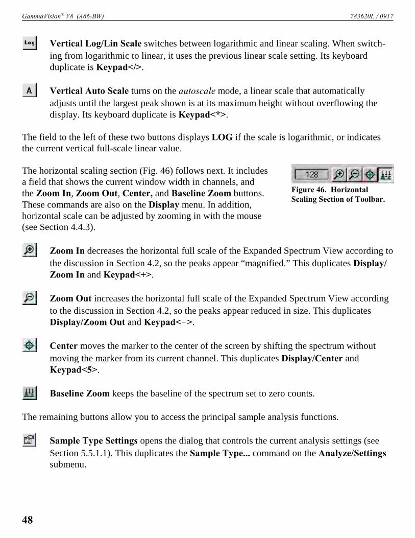
GammaVision® V8 (A66-BW) 783620L / 0917
Figure 46. HorizontalScaling Section of Toolbar.
Vertical Log/Lin Scale switches between logarithmic and linear scaling. When switch-
ing from logarithmic to linear, it uses the previous linear scale setting. Its keyboardduplicate is Keypad</>.
Vertical Auto Scale turns on the autoscale mode, a linear scale that automatically
adjusts until the largest peak shown is at its maximum height without overflowing thedisplay. Its keyboard duplicate is Keypad<*>.
The field to the left of these two buttons displays LOG if the scale is logarithmic, or indicatesthe current vertical full-scale linear value.
The horizontal scaling section (Fig. 46) follows next. It includesa field that shows the current window width in channels, andthe Zoom In, Zoom Out, Center, and Baseline Zoom buttons.These commands are also on the Display menu. In addition,horizontal scale can be adjusted by zooming in with the mouse(see Section 4.4.3).
Zoom In decreases the horizontal full scale of the Expanded Spectrum View according to
the discussion in Section 4.2, so the peaks appear “magnified.” This duplicates Display/Zoom In and Keypad<+>.
Zoom Out increases the horizontal full scale of the Expanded Spectrum View according
to the discussion in Section 4.2, so the peaks appear reduced in size. This duplicatesDisplay/Zoom Out and Keypad<!>.
Center moves the marker to the center of the screen by shifting the spectrum without
moving the marker from its current channel. This duplicates Display/Center andKeypad<5>.
Baseline Zoom keeps the baseline of the spectrum set to zero counts.
The remaining buttons allow you to access the principal sample analysis functions.
Sample Type Settings opens the dialog that controls the current analysis settings (see
Section 5.5.1.1). This duplicates the Sample Type... command on the Analyze/Settingssubmenu.
48

783620L / 0917 4. DISPLAY FEATURES
Figure 47. Drop-Down DetectorList.
Figure 49.
Figure 48. Roll-OverToolbar Tool Tips.
Analyze Spectrum duplicates the Entire Spectrum in Memory... command on the
Analyze menu (see Section 5.5.4).
The right-most part of the toolbar is a drop-down list of the available Detectors (Fig. 47). Toselect a Detector or the buffer, click in the field or on the down-arrow beside it to open the list,then click the desired entry. The sidebar will register your selection. Finally, note that as youpause the mouse pointer over the center of a toolbar button, a pop-up tool tip box opens,describing the button’s function (Fig. 48).
4.4. Using the Mouse
The mouse can be used to access the menus, toolbar, and sidebars; adjust spectrum scaling; markand unmark peaks and ROIs; select Detectors; work in the dialogs — every function in Gamma-Vision except text entry. The following sections describe specialized mouse functions.
4.4.1. Moving the Marker with the Mouse
To position the marker with the mouse, move the pointer to thedesired channel in the Expanded Spectrum View and click theleft mouse button once. This will move the marker to the mouseposition. Click in the Full Spectrum View to move the expandedview to that place. This is generally a much easier way to movethe marker around in the spectrum than using the arrow keysand accelerators, although you might still prefer some keyboardfunctions for specific motions.
4.4.2. The Right-Mouse-Button Menu
Figure 49 shows the right-mouse-button (context) menu. To openit, position the mouse pointer in the spectrum display, click theright mouse button, then use the left mouse button to select fromits list of commands. Not all of the commands are available
49
GammaVision® V8 (A66-BW) 783620L / 0917
at all times, depending on the spectrum displayed and whether the rubber rectangle is active.Except for Undo Zoom In, all of these functions are on the toolbar and/or the menus (PeakInfo, Input Count Rate, and Sum are only on the Menu Bar, under Calculate). SeeSection 5.11 for more information on the commands.
4.4.3. Using the “Rubber Rectangle”
The rubber rectangle is used for selecting a particular area of interest within a spectrum. It canbe used in conjunction with the toolbar and right-mouse-button menu commands for manyfunctions. To draw a rubber rectangle:
! Click and hold the left mouse button; this anchors the starting corner of the rectangle.
! Drag the mouse diagonally across the area of interest. As you drag, the mouse will bedrawing a reverse-color rectangle bisected by the marker line to form a “crosshair”(Fig. 51). This makes it easy to select the center channel in the area of interest — forinstance, the center of an ROI you wish to mark or unmark, a portion of the spectrum tobe summed, or a peak for which you want detailed information.
! Release the mouse button to anchor the ending corner of the rectangle.
! Once the area of interest is marked, select the applicable command from the toolbar,menus, right-mouse-button menu, Status Sidebar, or keyboard.
4.4.4. Resizing and Moving the Full Spectrum View
! Resizing — Roll the mouse pointer over the side edge, bottom edge, or corner of thewindow until the pointer changes to a double-sided arrow (see Fig. 50). Click and dragthe edge of the window until it is the size you want, then release the mouse button.
! Moving — Roll the mouse pointer onto the top edge of the window until the pointerchanges to a four-sided arrow (see Fig. 50). Click and drag the window to its newlocation, and release the mouse button.
4.5. Buttons and Boxes
This section describes GammaVision’s radio buttons, indexing buttons, and checkboxes. Toactivate a button or box, just click it.
! Radio buttons (Fig. 53) appear on many GammaVision dialogs, and allow only one ofthe choices to be selected.
50

783620L / 0917 4. DISPLAY FEATURES
Figure 51. RubberRectangle Crosshair.
Figure 52. Checkboxes.
Figure 53. Radio Buttons.
! Checkboxes (Fig. 52) are another common feature, allowing one or more of the optionsto be selected at the same time.
! The ROI, Peak, and Library indexing buttons on the Status Side-bar are useful for
rapidly locating ROIs or peaks, and for advancing between entries in the library. Whenthe last item in either direction is reached, the computer beeps and GammaVision postsa no more entries message on the Supplementary Information Line.
! The indexing buttons are displayed in two different ways, depending on whether Gamma-Vision is in Detector or buffer mode, as shown in Fig. 54. However, they function thesame way in both modes. In buffer mode, the additional features are the ability to insertor delete an ROI with the Ins and Del buttons, respectively (located between the ROIindexing buttons); and to display the peak information for an ROI with the Info button(located between the Peak indexing arrows).
! The Library buttons are useful after a peak has been located to move forward orbackward through the library to the next closest library entry. Each button press advancesto the next library entry and moves the marker to the corresponding energy. If a libraryfile has not been loaded or the Detector is not calibrated, these buttons are disabled.
Figure 50. Two-Sided Pointer for Sizing Full SpectrumView, and Four-Sided Pointer for Moving Window.
51

GammaVision® V8 (A66-BW) 783620L / 0917
Figure 54.Detector mode,top; buffer mode,bottom).
HINT Instead of using the Peak buttons to move from a previouslyidentified peak, click the marker anywhere in the spectrumthen click the Library buttons to locate the entries closestin energy to that point. If a warning beep sounds, it meansthat all library entries have been exhausted in that directionor that the spectrum is not calibrated. In any case, if an appro-priate peak is available at the location of the marker, peakdata are displayed on the Marker Information Line at thebottom of the screen.
The ROI and Peak indexing buttons are duplicated by <Shift+ 7>/<Shift+ 6> and <Ctrl+ 7>/ <Ctrl+ 6>, respectively. The Librarybuttons are duplicated by <Alt+ 7>/<Alt+ 6>. The Del button func-tion is duplicated by the <Delete> key and Clear ROI on the menus andtoolbar. The Ins button has the same function as the <Insert> key andMark ROI on the menus and toolbar. The Info button duplicates theCalculate/Peak Info command, Peak Info on the right-mouse-buttonmenu, and double-clicking in the ROI.
The Spectrum navigation section of the sidebar is displayed when N42 filesare loaded into a Buffer window. Individual spectra from an N42 filecontaining multiple spectra can be accessed using the navigation buttons orby entering the spectrum index in the current spectrum field. The drop downlist allows the list of spectra in a multi-spectrum N42 file to be filtered bythe spectrum type available in N42 files including Any (all spectra),Background, Time Slice, Long Count, Known Sample, and Blank Sample.
4.6. Opening Files with Drag-and-Drop
GammaVision lets you open ORTEC spectrum (.SPC, .AN1, .CHN), library (.LIB), and region ofinterest (.ROI) files by dragging and dropping them from Windows Explorer into the Gamma-Vision window. A spectrum file opens in a buffer window, a library file is loaded as the workinglibrary, and the ROIs saved in an .ROI file are set in the currently active spectrum window.
4.7. Associated Files
Installing GammaVision registers the spectrum files in Windows so they can be opened fromWindows Explorer by double-clicking the filename. The spectrum files are displayed in GVPlot.These files are marked with a spectrum icon ( ) in the Explorer display. .JOB files ( ) are alsoregistered, and open in Windows Notepad.
52

5. MENU COMMANDS
This chapter describes all the GammaVision menu commands and their associated dialogs. Theaccelerator(s) (if any) are shown to the right of the command. The underlined letter for eachcommand indicates the (English version) quick-access key that can be used with the <Alt> key(e.g., the Recall... command on the File menu can be selected with <Alt + F>, <Alt + R>.) Theellipsis (...) following a command indicates that a dialog is displayed to complete the function.Finally, a small arrow (“<”) following a menu selection means a submenu with more selectionswill be shown. The menus and commands, in the order they appear on the menu bar, are:
File (page 56)Settings...Recall...SaveSave As...ExportImportPrintCompare...Save Plot...ExitAbout GammaVision...
Acquire (page 70)Acquisition Settings...Start <Alt + 1>Start/Save/ReportStop <Alt + 2>Clear <Alt + 3>Copy to Buffer <Alt + 5>List ModeQA
Settings...Measure BackgroundMeasure SampleStatus...Control Chart...
Download SpectraZDT Display Select <F3>MCB Properties...
Calibrate (page 103)Energy...
53

GammaVision® V8 (A66-BW) 783620L / 0917
Efficiency...Description...Recall Calibration...Save Calibration...Print Calibration...Calibration Wizard
Calculate (page 143)Settings...List Data Range...Peak InfoInput Count RateSumSmoothStrip...
Analyze (page 149)Settings <
Sample Type...Report Generator...Attenuation Coefficients <
Coefficient TableCalculate from Spectra
Geometry CorrectionPeak Background Correction <
Create PBCSelect PBC...Edit PBC...Print PBC...
Average EnergyIodine EquivalencyDAC (MPC)Gamma Total...
Peak SearchROI Report...Entire Spectrum in Memory...Spectrum on Disk...Display Analysis Results...Interactive in Memory...
Library (page 206)Select Peak...
54

783620L / 0917 5. MENU COMMANDS
Select File...Edit <
GammaVision Editor...Nuclide Navigator...
List...
Services (page 215)Job Control...Sample Description...Menu Passwords...Lock/Unlock Detector...Edit Detector List...
ROI (page 221)Off <F2> or <Alt + O>Mark <F2> or <Alt + M>UnMark <F2> or <Alt + U>Mark Peak <Insert>Clear <Delete>Clear AllAuto ClearSave File...Recall File...
Display (page 223)Detector... Ctrl + <Fn>Detector/Buffer F4 or Alt + 6Select Spectrum...Logarithmic Keypad(/)Automatic Keypad(*)Baseline ZoomZoom In Keypad(+)Zoom Out Keypad(-)Center Keypad(5)Full View Alt + F7Isotope MarkersPreferences <
PointsFill ROIFill AllFill SingletsFill Multiplet Peaks
55

GammaVision® V8 (A66-BW) 783620L / 0917
Figure 55. File Menu.
Fill Multiplet CompositesSpectrum Colors...Peak Info/Font Color...
Window (page 228)CascadeTile HorizontallyTile VerticallyArrange IconsAuto ArrangeMultiple Windows[List of open Detector and buffer windows]
Right-Mouse-Button Menu (Spectrum/Buffer Windows) (page 229)StartStopClearCopy to BufferZoom InZoom OutUndo Zoom InMark ROIClear ROIPeak InfoInput Count RateSumMCB Properties
5.1. File
5.1.1. Settings...
The File Settings dialog allows you to specify how the spectrumdata are saved, exported, and imported; and set the directories forall the major file types used by GammaVision.
5.1.1.1. General
The entries on this tab (see Fig. 56) control the default spectrumfile format and the default sample descriptors to be saved withthe spectrum. If you also activate the ask-on-save feature for oneor more of these sample descriptors, they will be presented to the
56

783620L / 0917 5. MENU COMMANDS
Figure 56. File Settings Dialog, General Tab.
operator before each spectrum is saved.
When you finish setting the para-meters in this dialog and click OK,these settings will be used untilchanged. For other adjustable para-meters, see Acquire/AcquisitionSettings... (Section 5.2.1) andAnalyze/Settings/Sample Type...(Section 5.5.1.1).
Save File Format
The file types are integer .CHN,integer.SPC, real (floating-point).SPC, ASCII .SPE, and .N42 (2006
and 2012 format). The .CHN and .SPC
files are binary structures described in the ORTEC Software File Structure Manual for DOS andWindows® Systems (P/N 753800, hereinafter called the File Structure Manual), available on theGammaVision start menu.
The .CHN file format contains basic acquisition information including the live time, real time,acquisition start time, MCB and sample descriptions, and energy calibration (if any); but doesnot contain the analysis parameter data, the complete calibration, or other data needed fornuclide analysis.
The two .SPC formats contain all of the parameters from the .CHN files as well as the completecalibration records, analysis parameters, hardware parameters, and other data needed forspectrum analysis. The two formats are identical except for the format of the spectrum data. Theinteger format is the current standard and stores the spectrum as 4-byte integers. The floating-point format is for backward compatibility with legacy software and uses the 4-byte exponentialformat.
The ASCII .SPE format is used by the Comprehensive Test Ban Treaty Organization (CTBTO).
The .N42 format is XML with tags and descriptions taken from the respective ANSI N42.42standards.
57

GammaVision® V8 (A66-BW) 783620L / 0917
Ask On Save Options
Use these fields to enter the default sample descriptors to be saved with the spectrum. If you alsomark the corresponding Ask on Save checkbox, the default value entered here will be presentedfor acceptance or modification when the spectrum is saved.
Sample Description allows you to designate the default sample description to be saved with thespectrum (128-character maximum for .SPC files; 63 characters for .CHN files). Marking the Askon Save checkbox lets you enter the common descriptors for a group of samples ahead of time,then add the unique descriptors sample-by-sample after each acquisition.
If the output activity is to be normalized to a volume or weight (or any other factor), the defaultSample Size can be entered here along with the reporting units and an optional 1-sigma uncer-tainty (+/-) between 0% and 1000%. This will normalize the activity, and the report will be innormalized units. This normalization is in addition to the normalization done by the Multiplierand Divisor fields on the System tab of the Sample Type Settings dialog(Analyze/Settings/Sample Type...).
The Collection Date and Time are the time used in the decay correction. If the decay correctionis enabled (see the Sample tab of the Sample Type Settings dialog), this is the date used in thecorrection formula.10
Sample Start/End Time
These dates/times are the start time of the sample collection and the stop time of the sample col-lection. For example, for air filters, the start time is the time when the air flow is started, and thestop time is when the air flow is stopped. These times are used to calculate the buildup of theactivity in the sample. It is assumed that the spectrum is not collected during the buildup time.The correction for the buildup is given in Section 5.8.4.
5.1.1.2. Export
The Export tab (Fig. 57) lets you specify the program, arguments, and file directory to be usedwhen the Export... command is selected. If this computer has the DataMaster Spectrum File
NOTE Before using the Acquire/Download Spectra command, or the Move feature on asupported instrument’s Field Data tab, be sure to select the Save File Format youwish to use for the downloaded spectra.
10If the collection date and time is before that of the spectrum acquisition, the spectrum will be activity correctedback to the sample collection time. While this is the normal use of this input, if the collection date and time isafter the acquisition time, the decay correction will be made forward in time.
58

783620L / 0917 5. MENU COMMANDS
Figure 57. Export Tab.
Figure 58. ExportArgument Macros.
Format Translator (A49-B32) installed, the Use DataMaster and Export As fields will be activeand you can use the DataMaster export (and import) functions.
Choose any Export Program11
that can accept the spectrum file-name as an argument on the com-mand line. Click on Browse... toautomatically select the completeproper path for the program.
Arguments
The Arguments to the programcan be entered as characterstrings or you can select fromthe list of “macros” shown inFig. 58. The list is displayed byclicking on the arrow button tothe right of the Arguments field.Entries (macros or direct) mustbe separated by spaces to be read as separate arguments.
! File Path Name — This will insert the complete file pathname (e.g., c:\user \spectrum\
test.chn) into the dialog box. This filename is the one chosen in the Export command’s file-recall dialog.
! File Base Name — This will insert the file path name with-out the extension (e.g., c:\user\ spectrum\test) into thedialog. The filename is the name selected in the Exportcommand’s dialog. The extension can be entered manuallyafter the macro (e.g., $(FullBase).CHN) into the dialog. Notethat the “dot” ( . ) must also be entered. Related filenamescan also be made by adding characters before the “dot”(e.g., $(FullBase)A.CHN).
! Short Name — This will insert the filename (e.g., test.CHN) into the dialog box. The file-name is the name selected in the Export command’s dialog. File names can be constructed as$(file base).$(file extension).
11Any executable program that can be executed from the Windows Run command can be selected, includingDOS batch commands.
59

GammaVision® V8 (A66-BW) 783620L / 0917
Figure 59. The InitialCharacter Macros.
Figure 60. Choose the DataMasterExport File Type.
! Short Base — This will insert the base filename (e.g., test) into the dialog box. The file basename is the name selected in the Export command’s dialog.
! File Extension — This will insert the file extension (e.g., CHN) into the dialog box. The fileextension is the file type for the file chosen in the Export command’s dialog. Note that the“dot” is not included. Any manually inserted input of the macro form ($(xxx)) will beincluded in the argument list without changes.
Initial Directory
The initial directory for the program to use can be specified asdirectly entered character strings or the user can select fromthe list of macros in Fig. 59. The list is displayed by clickingon the arrow button to the right of the Initial Directory field.
! File Directory — This is the directory in which the fileselected with the File/Export command is located (e.g.,c:\user\spectrum\).
! Program Directory — This is the directory for the conversion program. It is shown inthe first entry of this dialog.
! GammaVision Directory — This is the directory where the GammaVision program isstored. By default, this is C:\Program Files\GammaVision.12
! Current Directory — This is the current default directory for Windows.
Run Options
These three radio buttons (Minimized, Maximized, and Normal Window) are used to select thewindow for the program. If the program does not have any user dialogs, any option can beselected. If the program needs user inputs, Normal Windowshould be selected.
Use DataMaster
To use DataMaster as the export program, mark thecheckbox then select the file type to be exportedfrom the Export As list. Figure 60 shows the list of
12C:\Program Files (x86) on 64-bit Windows computers.
60

783620L / 0917 5. MENU COMMANDS
Figure 61. Import Tab.
Figure 62. ImportArguments.
supported file types. To use the Export Program specified in the upper half of the dialog, justunmark the Use DataMaster box.
5.1.1.3. Import
The Import tab (Fig. 61) lets you specify the program, arguments, file directory, and default fileextension to be used when the Import... command is executed. If this computer has the Data-Master Spectrum File Format Translator installed, the Use DataMaster and Default File Typefields are active and you can use the DataMaster import (and export) functions.
Choose any Import Program that can accept the spectrum filename on the command line. ClickBrowse... to select the complete proper path for the program.
Arguments:
The arguments to the program can be specified as directly enteredcharacter strings or you can select from the list of macros shownin Fig. 62. The list is displayed by clicking on the arrow buttonto the right of the Arguments field. The entries (macros or direct)must be separated by spaces to be read as separate arguments. Thearguments on this menu are described in Section 5.1.1.2 under“Arguments” (page 59), except that here they refer to the file-name selected for importation with the File/Import command.
61

GammaVision® V8 (A66-BW) 783620L / 0917
Figure 63. ImportMacros.
Figure 64. Choose the DataMasterImport File Type.
Initial Directory
Specify the initial directory for the program to use either withdirectly entered character strings or by selecting from the listof macros shown in Fig. 63. The list is displayed by clicking onthe arrow button to the right of the Initial Directory field. Thedirectories on this menu are described in Section 5.1.1.2 under“Initial Directory” (page 60), except that the reference to file-name applies to the file selected for importationwith the File/Import command.
Default
The default extension entered here is used as the extension for the filename in the filename entrydialog. For example, if TXT is entered, then the name list in the entry dialog will be *.TXT.
Run Options
These three radio buttons (Minimized, Maximized, and Normal Window) are used to select thewindow for the program. If the program does not have any user dialogs, any option can beselected. If the program needs user inputs, Normal Window should be selected.
Use DataMaster
To use DataMaster as the import program, mark thecheckbox then select the file type to be imported fromthe Default File Type list. Figure 64 shows the listof supported file types. To use the Import Programspecified in the upper half of the dialog, just unmarkthe Use DataMaster box.
5.1.1.4. Directories
This tab (Fig. 65) gives you the option of desig-nating where GammaVision’s various file typesshould be stored. Otherwise, all spectra, .ROI files,libraries, .JOB files, reports, correction table files,sample type files, and calibrations will be storedin C:\User. When you generate any of Gamma-
62

783620L / 0917 5. MENU COMMANDS
Figure 65. Directories Tab.
Vision’s many File Types, the program reads the file extension and stores it according to thelocation(s) specified on this tab. For instance, if you specify a location for the Spectra file type,all .SPC, .CHN, .SPE and .N42 files will be saved there by default. Similarly, if you specify alocation for the Table Files file type, GammaVision will save your energy (.ENT) and efficiency(.EFT) calibration tables and table for DAC (.DAC), geometry (.GEO) and other corrections inthat folder.
To change the path (Location) of a particular File Type, click the desired file type, thenModify.... This will open a standard file-recall dialog. Choose the desired location, creating anew folder if necessary, and click Open. When all path changes have been completed, click OKto put them into effect or else Cancel to retain the previous settings.
5.1.2. Recall...
This command reads a spectrum or List Mode file into a new buffer window. It opens a standardWindows file-open dialog (Fig. 66), allowing you to select the file to be recalled. The spectrumfiles are created by GammaVision’s Save and Save As... functions and by any other programsthat can produce the .CHN, .SPC, .SPE, .N42, or .LIS format (e.g., MAESTRO). The buffer isresized to the memory size of the recalled spectrum.
Note the Show Description checkbox on the lower left of the dialog. Mark this to display thesample description, format, and spectrum size of each file without having to open it.
If the maximum eight buffer windows are currently open, GammaVision will ask if you wish to
63

GammaVision® V8 (A66-BW) 783620L / 0917
Figure 66. Recall a Spectrum File.
Figure 67. Save As.
close the oldest buffer. Answering Nowill cancel the recall operation and theoldest buffer will remain onscreen.Answering Yes will close the oldestbuffer and open a new buffercontaining the recalled file. If theoldest buffer contains data that havenot been saved, a warning dialog willfirst ask if the data should be saved.Click Yes to save and No to closewithout saving.
When the spectrum is successfullyrecalled, GammaVision loads itsdescriptors (start time, live time,real time, Detector and sampledescriptions) and calibration infor-mation (if any), and displays the filename on the title bar. For spectrum files containing multiplespectra (such as ZDT mode in supported ORTEC instruments), both spectra are automaticallyrecalled.
5.1.3. Save/Save As...
These functions open a standardWindows file-save dialog (Fig. 67)so you can save the current spectrumto disk. Use Save As... to renamean existing spectrum. If you attemptto overwrite an existing filename, amessage box opens asking you toverify the entry or cancel the save.Clicking OK overwrites the exist-ing file. After the disk file has beensaved, its filename is displayed onthe title bar.
PHA Mode Spectra — The defaultformat is specified on the Generaltab under File/Settings... (Section 5.1.1.1); see that section for a brief description of the .CHN,.SPC, .SPE, and .N42file types. Note that you can select any of these file types at the time yousave the file, and the save dialog will remember the most recent file type used. or hardware withmultiple spectra (such as ZDT mode in the DSPEC Pro), both spectra will be saved in the file.
64

783620L / 0917 5. MENU COMMANDS
Figure 68. The Export Spectrum File Dialog.
PHA mode spectra cannot be saved in the .LIS (List Data) format.
List Mode Spectra — By default, the Save and Save As... commands offer to save List Modespectra in .LIS format, however, you can also save this data in any of the other file formats. Notethat the structure and contents of .LIS files is instrument-dependent (see the associated hardwaremanual for more information), but includes the Detector’s current calibration and sampledescription.
5.1.4. Export...
The Export... function is used towrite spectra in formats other thanthe usual formats, or to performother functions such as plotting orprinting the spectrum directly. Theexport program is specified on theExport tab under File/Settings...,as discussed in Section 5.1.1.2. Theprogram can be one of the programssupplied or can be user-supplied.When selected, the Export Spec-trum File dialog, shown in Fig. 68,is displayed. Choose the filenameof the spectrum to be exported.
The currently displayed spectrummust be saved to disk before it canbe exported. If the currently displayed spectrum has already been stored to disk, that filename isthe default. Any file can be selected. The file is then read and the output file is writtenby the program.
The Export... function is not available for a second file until the first file has been exported andthe export program has stopped execution.
Export... can also be used to generate hardcopy plots. To do this, select the GVPlot program(supplied with GammaVision) as the export program. When Export... has been selected, theGVPlot program will be executed. If the -P switch is specified on the command line (see Sec-tions 5.1.1.2 and 11.1.5), the program will plot the spectrum and exit automatically.
5.1.5. Import...
The Import function is used to read spectrum files that are not in one of the usual formats (e.g.,
65
GammaVision® V8 (A66-BW) 783620L / 0917
.CHN or .SPC). The import program is specified on the Import tab under File/Settings..., asdiscussed in Section 5.1.1.3. The program can be one of the programs supplied or can be user-supplied. This command opens a standard Windows file-open dialog so you can select the file-name. The file is then read and a spectrum file is written to the specified directory. Gamma-Vision attempts to read this file (in .CHN or .SPC format) and displays the spectrum. If theImport program does not generate a file that GammaVision can read, no spectrum is displayed.
5.1.6. Print
The Print function does one of the following:
! If the marker is in an ROI, the data contents of the ROI channels are printed.! If the marker is not in an ROI, the contents of channels in the expanded view are printed.
A standard file-print dialog opens, allowing you to print the output or save it in a disk file (markthe Print to file box). The data are formatted at seven channels per line with the channel numberon the left.
5.1.7. Compare...
This function allows you to compare the currently displayed spectrum with an existing spectrumfile. When the file-recall dialog opens, select the desired spectrum file. Both spectra will bedisplayed together as illustrated in Fig. 69, and the title bar will list both spectrum filenames.
The Compare spectrum is offset from the starting spectrum, and can be moved up and downincrementally with the <Shift + 8> and <Shift + 9> accelerators. In addition, the vertical scaleof both spectra can be simultaneously changed with <8> and <9>. Note that the Comparespectrum’s ROIs (if any were saved with the file) are not marked in this mode.
Figure 70 portrays a zoomed-in portion of two comparison files. In this illustration, the startingspectrum is displayed in color (1), the Compare spectrum is shown in color (2), the starting spec-trum’s ROIs are marked in color (3), and the portion of the starting spectrum that exceeds theCompare spectrum is indicated by color (4). These colors — called Foreground, Compare,ROI, and Composite, respectively — are chosen on the Color Preferences dialog discussed inSection 5.9.12.2.
Press <Esc> to leave Compare mode.
66

783620L / 0917 5. MENU COMMANDS
Figure 69. Compare Mode Screen.
Figure 70. SpectrumColors in CompareMode.
5.1.7.1. Comparing ZDT Spectra with <Shift + F3>
The Compare feature also works for MCBs that support theZero Dead Time (ZDT) correction,3 which generates two spectraper acquisition; and for ZDT spectrum files, which store the twospectra.13 You can also compare a ZDT Mode spectrum to a non-ZDT spectrum file, however, note that the ZDT MCB or file mustbe opened first to enable the View ZDT Corrected command(which allows you to toggle between the CORR and ERR spectrain the file; the shortcut key is <F3>). Then use the Comparecommand to open the non-ZDT file.
13See Sections 5.2.11.4 and 5.2.10 for explanations of ZDT mode and the View ZDT Corrected command,respectively.
67

GammaVision® V8 (A66-BW) 783620L / 0917
Figure 71. Spectrum Bitmap Image.
When you issue the Compare command and select another ZDT spectrum file, that file opensin the current mode of the starting spectrum, so you are viewing ERR/ERR or ZDT/ZDT. UseView ZDT Corrected to toggle both spectra in unison between ERR/ERR and ZDT/ZDT. Tohold the starting spectrum in the current view mode and switch the Compare spectrum to theopposite view, use <Shift + F3>. View ZDT Corrected then allows you to switch between theERR/ZDT and ZDT/ERR comparisons. (It is also possible to do this with a non-ZDT Comparespectrum, in which case <Shift + F3> toggles between the single live-time-corrected spectrumand an empty spectrum baseline.)
5.1.8. Save Plot...
This command is active for buffer and Detector windows when spectrum data is present. Usingthe current color, titling, and x-/y-axis scaling options set in GVPlot (Section 11.1), it saveseither a native bitmap (.BMP) or JPEG (.JPG) image of the currently displayed spectrum(Fig. 71).
68

783620L / 0917 5. MENU COMMANDS
Figure 72. About GammaVision.
The entire spectrum is saved (to save or print a zoomed portion, use the GvPlot program). Astandard file-save dialog opens allowing you to choose the image format and file name andlocation. The image is scaled to fit on 8.5 in. × 11 in. paper in landscape orientation. GvPlotcreates the images with a resolution of 100 D.P.I. so the full image resolution is 1100 × 850pixels.
5.1.9. Exit
This terminates the GammaVision program. If the buffer contains a spectrum that has not beensaved, a warning message gives you a file-save option. Any JOBs are terminated. All activeMCBs continue to acquire data until the presets are met.
5.1.10. About GammaVision...
Figure 72 shows the About box for GammaVision. It provides software version information thatwill be useful should you need customer support.
Click the Visit ORTEC OnLine button to browse our website includes our product catalog,application notes, technical papers, information on training courses, and access to our GlobalService Center.
69

GammaVision® V8 (A66-BW) 783620L / 0917
Figure 73. Acquire Menu.
Figure 74. Acquisition Settings.
5.2. Acquire
The Acquire menu is shown in Fig. 73. Access to the variousfunctions depends on whether the a Detector or buffer windowis currently active (for example, if a buffer window is active theDetector controls are disabled and MCB Properties... is read-only). The List Mode, Download Spectra and View ZDT Cor-rected commands are available only for supported hardware(which is listed in the discussion for each of these functions).
NOTE In some cases, a Detector option might be disabledbecause it is not supported by the current Detector(while it might still be valid for some other Detectorin the system, or for this Detector under differentconditions).
5.2.1. Acquisition Settings...
This command opens theAcquisition Settings dialog(Fig. 74), which allows youto control a number of ques-tions that can be “asked onstart” (when a Detector isstarted) and their defaultvalues.
To take advantage of themulti-detector capability,the Group Acquisitionssettings apply to the Start,Stop, Start/Save/Report,and Clear commands. Youcan control acquisition in alldisplayed Detectors simulta-neously (All MCBs) or oneDetector at a time (CurrentMCB); or be asked if youwish to apply an acquisitioncommand to one or all dis-played Detectors (Prompt).
70

783620L / 0917 5. MENU COMMANDS
The Spectrum Location field gives you the option of saving each Detector’s spectra to differentfolders (in the example in Fig. 74, this Detector’s spectra will be stored in C:\User\EDF Det 1\).If you leave this field blank, all spectra for this Detector are stored in the folder designated onthe Directories tab under File/Settings... (Section 5.1.1.4).
NOTE To start all Detectors simultaneously, you must turn off all Ask on Start Options. Thisis explained in Section 5.2.1.2.
5.2.1.1. Start/Save/Report
For the Start/Save/Report function, you must select Clear at Start, which automatically clearsthe Detector before acquisition starts, specify the base filename of the save file (File Prefix), anddecide whether the filename is to be automatically incremented after each use (Auto-Incre-ment). The File Prefix can be up to eight alphanumeric characters. However, if Auto-Incre-ment is specified, the limit is seven characters. The first one to seven characters of the filenameare the file prefix. The remaining characters are the sequence numbers. This starts with the num-ber entered in the Save File # field. The number increments to the number of allowed characters(e.g., AAAAAA99) then restarts at zero (e.g., AAAAAA00). The prefix must be short enough toaccommodate the number of expected files. The filename is expanded to eight characters withzeros. If the Auto-Increment box is checked, the filename will be incremented by 1 each timethe Start/Save/Report is done. For example, if 0 were entered for prefix GVX, the first filenamewould be GVX00000, the second would be GVX00001, and so on.
If the Auto-Increment box is not checked, the same file is used for every analysis and theprevious data are overwritten with each Start/Save/Report. The analysis uses the settings fromAnalyze/Settings/Sample Type... (Section 5.5.1.1).
5.2.1.2. Ask on Start Options
Each Detector has its own suite of Ask on Start parameters. When you start a Detector, Gamma-Vision prompts for any Ask on Start options that have been turned on. As soon as the promptsfor a specific Detector are satisfied, that Detector begins acquisition. If you choose Cancel forany of these parameters, the remaining ask-on-start sequence for that Detector terminates andacquisition for that Detector is canceled.
This also applies when starting all Detectors simultaneously (All MCBs). If the Ask on StartOptions have been turned on for any Detector in the group, GammaVision steps through the listof Detectors to be started, and if any ask-on-start parameters are active, the software prompts forthem. As soon as the ask-on-start prompts are satisfied for a particular Detector, acquisition inthat Detector begins immediately. Therefore, to start all Detectors simultaneously, you must turnoff all ask-on-start options.
71

GammaVision® V8 (A66-BW) 783620L / 0917
Sample Type Defaults
The sample type file, which contains many of the parameters needed for analysis and acquisition,can be specified here. The file is created in the Sample Type Settings dialog, Section 5.5.1.1.When specified, the file is read and the values in it are the defaults for this dialog. If the Ask onStart box is checked, GammaVision will ask for the sample type when Detector acquisitionstarts, and the values in that file will be used. Click Browse... to show the available files.
Acquisition Presets
If the Ask on Start box is checked, the presets are asked when the Detector is started; the dialogis the same as the Preset tab for this Detector’s MCB Properties dialog. Only the non-zeropresets can be changed during the start.
Sample Description
The sample description can be entered here, and it can also be asked for when the spectrum issaved. If the Ask on Start box is checked, the description entered here will be presented as thedefault at the start of data acquisition. This feature is handy when processing a number of similarsamples; the common part of the description can be entered here, and the unique descriptors canbe added on start.
Sample Size
If the output activity is to be normalized to a volume or weight (or any other factor), the samplequantity can be entered here, along with an optional 1-sigma uncertainty (+/-) between 0% and1000%. The reporting units are entered, according to the sample type, on the System tab underAnalyze/ Settings/Sample Type... (page 152). This will normalize the activity and the reportwill be in normalized units. This normalization is in addition to any normalization done by themultiplier and divisor on the Analysis tab under Analyze/Settings/Sample Type... (page 152).
Collection Date and Time
If the decay correction is enabled (see the Sample tab under Analyze/Settings/Sample Type...,Section 5.5.1.1), the collection date and time are used in the correction formula.14
14If the collection date and time is before that of the spectrum acquisition, the spectrum will be activity-correctedback to the sample collection time. While this is the normal use of this input, if the collection date and time isafter the acquisition time, the decay correction will be made forward in time.
72

783620L / 0917 5. MENU COMMANDS
Figure 75. Start One or All DisplayedDetectors.
Sample Start/Stop Time
These dates/times are the start time of the sample collection and the stop time of the samplecollection. For example, for air filters, the start time is the time when the air flow is started andthe stop time is when the air flow is stopped. These times are used to calculate the build-up ofthe activity in the sample. It is assumed that the spectrum is not collected during the build-uptime. The correction for the build-up is given in Section 5.8.4.
5.2.2. Start
Based on the Group Acquisitions setting in theAcquisition Settings dialog, Start simultaneouslybegins acquisition in all displayed Detectors (AllMCBs) or one Detector at a time (Current MCB);or asks if you wish to begin data collection in oneor all displayed Detectors (Prompt), as shown inFig. 75.
Any warnings arising from problems detected at the hardware level will appear in a message boxor on the Supplemental Information Line at the bottom of the display. The Detector can also bestarted with the <Alt + 1> accelerator, the Start Acquisition button on the toolbar, or the Startcommand on the right-mouse-button menu. If the Detector is already started or if GammaVisionis in buffer mode, this command is disabled.
See Section 5.2.1.2 for a discussion of how ask-on-start options can affect the start of dataacquisition.
5.2.3. Start/Save/Report
This command performs all three functions without user intervention. The Start is the same asthe Start above, Save is the same as File/Save (using the filename in the Acquire/AcquisitionSettings... dialog), and Report is the same as Analyze/Entire spectrum in memory. Based onthe Group Acquisitions setting in the Acquisition Settings dialog, Start/Save/Report simul-taneously begins acquisition in all displayed Detectors (All MCBs) or one Detector at a time(Current MCB); or asks if you wish to begin data collection in one or all displayed Detectors(Prompt).
5.2.4. Stop
Stop terminates data collection in the active Detector window. The Detector can also be stoppedwith the accelerator <Alt+ 2>, the Stop Acquisition button on the toolbar, and the Stop com-mand on the right-mouse-button menu. Based on the Group Acquisitions setting in the Acquisi-tion Settings dialog, Stop simultaneously halts acquisition in all displayed Detectors (All
73

GammaVision® V8 (A66-BW) 783620L / 0917
MCBs) or one Detector at a time (Current MCB); or asks if you wish to stop data collection inone or all displayed Detectors (Prompt).
5.2.5. Clear
Clear erases the spectral data and the descriptors (e.g., real time, live time, start time) for thecurrently active Detector or buffer window. The presets are not altered. Because the GroupAcquisitions setting in the Acquisition Settings dialog applies to Detector windows only, thiscommand operates differently in Detector windows than in buffer windows. If a buffer windowis active, Clear erases only that buffer window, regardless of how many buffer windows areopen. However, if a Detector window is active, Clear simultaneously clears all displayed Detec-tors (All MCBs), erases only the active Detector window (Current MCB); or asks if you wishto clear one or all displayed Detectors (Prompt).
This command might not operate on some types of Detectors when they are collecting data. Thedata can also be cleared with <Alt+ 3>, the Clear Spectrum button on the toolbar, or the Clearcommand on the right-mouse-button menu.
5.2.6. Copy to Buffer
The Copy to Buffer function transfers the data and descriptors (e.g., live time, real time), fromthe active Detector window to a new buffer window. This function can also be performed with<Alt + 5> or the Copy to Buffer command on the right-mouse-button menu.
5.2.7. List Mode
This toggles the current Detector’s data acquisition mode between PHA mode and list mode(Section 1.6). This function can also be performed with the List Mode toolbar button.
5.2.8. QA
This is explained in Chapter 8, “Quality Assurance.”
5.2.9. Download Spectra...
This command supports standalone MCBs such as Detective®-family instruments, trans-SPEC®,digiDART®, and the legacy DART®, and is used to download the spectra from the MCB to thecomputer disk. Note that downloading the spectra does not erase them from the MCB.
The files are stored in the directory and spectrum file format specified in the dialog under File/Settings (Section 5.1.1), and are named according to this format:
sss iiiiiiii ddddddddd ttttttttt.ext
74
783620L / 0917 5. MENU COMMANDS
where:sss is the sequence number as shown on the digiDART spectrum list display
or the storage sequence in other supported MCBs.
iiiiiiii is the ID string entered on the digiDART when the spectrum was savedand shown on the digiDART spectrum list display or the text string fromthe barcode reader in the DART.
ddddddddd is the date the spectrum was collected, as recorded in the MCB.
ttttttttt is the time the spectrum was collected, as recorded in the MCB.
ext is the extension for the file type selected.
If any Ask on Save Options are set in the File Settings dialog, they are asked for each spectrumindividually. Note that if you cancel an ask-on-save prompt for a particular spectrum, anyremaining ask-on-save prompts for that spectrum are not displayed, and the spectrum is notsaved to disk.
NOTE Before downloading, make sure the current conversion gain setting for this MCB (seethe ADC tab under Acquire/MCB Properties...) is the same as or greater than the con-version gain of the stored spectra; otherwise, the downloaded spectra will be truncatedat the current conversion gain setting. For example, if a digiDART was used to acquire8k spectra in the field and the current conversion gain setting is 4k, only the first4096 channels of data in each spectrum will be downloaded. See also the spectrum fileformat NOTE on page 57.
5.2.10. ZDT Display Select
This command is active (1) for a Detector that supports ZDT Mode and has one of the ZDTmodes enabled on the ADC tab under Acquire/MCB Properties..., and (2) a ZDT spectrum filerecalled into a buffer window.
When the Detector is in the CORR_ERR ZDT mode (the NORM_CORR mode is typically notused), two spectra are collected: the uncertainty spectrum, labeled ERR; and the zero-dead-timecorrected spectrum, labeled ZDT (see the discussion in Section 5.2.11.4 for more information).The spectrum label is displayed in the upper-right corner of the Full Spectrum View, as shown inFig. 76.
The View ZDT Corrected command (duplicated by the shortcut <F3>) allows you to toggle
75

GammaVision® V8 (A66-BW) 783620L / 0917
Figure 76. Comparison of Uncertainty and ZDT Spectra Showing Labels inFull Spectrum View.
between the two spectra. Note that in the CORR_ERR ZDT mode, the status sidebar does notdisplay a live-time readout for either the ERR or ZDT spectra.
5.2.11. MCB Properties...
CONNECTIONS applications use a uniform dialog for data acquisition setup, accessed with theAcquire/MCB Properties... command. The property pages for the DSPEC-50 are describedhere. To see the Properties dialog for other CONNECTIONS MCBs, refer their respective hardwaremanuals.
Depending on the currently selected Detector, the Properties dialog displays several tabs of hard-ware controls that may include ADC setup parameters, acquisition presets, high-voltage controls,amplifier gain adjustments, gain and zero stabilizers, pole-zero and other shaping controls, theInSight™ Virtual Oscilloscope, digital noise-suppression filters, and radionuclide detectionreports. In addition, some MCBs monitor conditions such as detector temperature, external inputstatus, alpha chamber pressure, charge remaining on batteries, and the number of spectra collec-ted in remote mode, which are reported on a Status tab. Simply move from tab to tab and setyour hardware parameters, then click Close. Note that as you enter characters in the data entryfields, the characters will be underlined until you move to another field or until 5 seconds havelapsed since a character was last entered. During the time the entry is underlined, no other
76
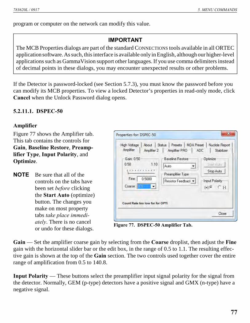
783620L / 0917 5. MENU COMMANDS
Figure 77. DSPEC-50 Amplifier Tab.
program or computer on the network can modify this value.
If the Detector is password-locked (see Section 5.7.3), you must know the password before youcan modify its MCB properties. To view a locked Detector’s properties in read-only mode, clickCancel when the Unlock Password dialog opens.
5.2.11.1. DSPEC-50
Amplifier
Figure 77 shows the Amplifier tab.This tab contains the controls forGain, Baseline Restore, Preamp-lifier Type, Input Polarity, andOptimize.
NOTE Be sure that all of thecontrols on the tabs havebeen set before clickingthe Start Auto (optimize)button. The changes youmake on most propertytabs take place immedi-ately. There is no cancelor undo for these dialogs.
Gain — Set the amplifier coarse gain by selecting from the Coarse droplist, then adjust the Finegain with the horizontal slider bar or the edit box, in the range of 0.5 to 1.1. The resulting effec-tive gain is shown at the top of the Gain section. The two controls used together cover the entirerange of amplification from 0.5 to 140.8.
Input Polarity — These buttons select the preamplifier input signal polarity for the signal fromthe detector. Normally, GEM (p-type) detectors have a positive signal and GMX (n-type) have anegative signal.
IMPORTANT
The MCB Properties dialogs are part of the standard CONNECTIONS tools available in all ORTECapplication software. As such, this interface is available only in English, although our higher-levelapplications such as GammaVision support other languages. If you use comma delimiters insteadof decimal points in these dialogs, you may encounter unexpected results or other problems.
77

GammaVision® V8 (A66-BW) 783620L / 0917
Baseline Restore — This is used to return the baseline of the pulses to the true zero betweenincoming pulses. This improves the resolution by removing low frequency noise from dc shiftsor mains power ac pickup. The baseline settings control the time constant of the circuit thatreturns the baseline to zero. There are three fixed choices (Auto,15 Fast, and Slow). The fastsetting is used for high count rates, the slow for low count rates. Auto adjusts the time constantas appropriate for the input count rate. The settings (Auto, Fast, or Slow) are saved in theDSPEC-50 even when the power is off. The time constant can be manually set on the InSightdisplay (see the discussion beginning on page 98).
You can view the time when the baseline restorer is active on the InSight display as a Markregion (see the Marks discussion, p. 100). In the automatic mode, the current value is shown onthe InSight sidebar. For a low-count-rate system, the value will remain at about 90.
Preamplifier Type — Choose Transistor Reset or Resistive Feedback preamplifier operation.Your choice will depend on the preamplifier supplied with the germanium detector being used.
Optimize
The DSPEC-50 is equipped with both automatic pole-zero logic16 and automatic flattop logic.17
The Start Auto (optimize) button uses these features to automatically choose the best pole-zeroand flattop tilt settings. Note that if you selected Transistor Reset as the Preamplifier Type forthis DSPEC-50, optimization does not perform the pole zero.
NOTE You cannot optimize with LFR mode enabled; see Section 5.2.11.1.
As with any system, the DSPEC-50 should be optimized any time the detector is replaced or ifthe flattop width is changed. For optimization to take place, the DSPEC-50 must be processingpulses. The detector should be connected in its final configuration before optimizing. A countrate guidance message on the lower-left of the Amplifier page will help you position a radio-active source to deliver the correct count rate for optimization. The Start Auto optimizationbutton will be disabled (gray) until the count rate is suitable.
Select either the Resistive Feedback or Transistor Reset option and click on Start Auto. Theoptimize command is sent to the DSPEC-50 at this time and, if the DSPEC-50 is able to start the
15U.S. Patent 5,912,825.
16U.S. Patent 5,872,363.
17U.S. Patent 5,821,533.
78

783620L / 0917 5. MENU COMMANDS
Figure 78. DSPEC-50 Amplifier 2 Tab.
operation, a series of short beeps sounds to indicate that optimization is in progress. Whenoptimizing is complete, the beeping stops.
During optimization, pole zeroes are performed for several rise-time values and the DSPEC-50 iscycled through all the rise time values for the determination of the optimum tilt values. Allvalues for all the combinations are then saved in the DSPEC-50, so you do not need to optimizefor each possible rise time. Optimization can take from 1 to 10 minutes depending on count rate,but typically takes 5 minutes.
NOTE Be sure to repeat the optimization if you change the flattop width.
The effect of optimization on the pulse can be seen in the InSight mode, on the Amplifier 2 tab.Note, however, that if the settings were close to proper adjustment before starting optimization,the pulse shape may not change enough for you to see. (In this situation, you also may not noticea change in the shape of the spectrum peaks.) The most visible effect of incorrect settings ishigh- or low-side peak tailing or poor resolution.
Amplifier 2
Figure 78 shows the Amplifier 2tab, which accesses the advancedshaping controls including theInSight Virtual Oscilloscope mode.
The many choices of Rise Timeallow you to precisely control thetradeoff between resolution andthroughput. The value of the risetime parameter in the DSPEC-50is roughly equivalent to twice theintegration time set on a conven-tional analog spectroscopy amp-lifier. Thus, a DSPEC-50 valueof 12 ìs corresponds to 6 ìs in aconventional amplifier. Startingwith the nominal value of 12.0, you should increase values of the rise time for better resolutionfor expected lower count rates, or when unusually high count rates are anticipated, reduce therise time for higher throughput with somewhat worse resolution.
The DSPEC-50 Rise Time ranges from 0.8 ìs to 23.0 ìs. Once the unit has been optimizedaccording to Section 5.2.11.1, you can use any Rise Time without having to re-optimize. Themost recent settings are saved in the DSPEC-50 firmware even when the power is turned off.
79

GammaVision® V8 (A66-BW) 783620L / 0917
For the more advanced user, the InSight mode allows you to directly view all the parameters andadjust them interactively while collecting live data. To access the InSight mode, go to theInSight section on the Amplifier 2 tab and click on Start. The InSight mode is discussed inmore detail in Section 5.2.11.5.
The Rise Time value is for both the rise and fall times; thus, changing the rise time has the effectof spreading or narrowing the quasi-trapezoid symmetrically.
The Flattop controls adjust the top of the quasi-trapezoid. The Width adjusts the extent of theflattop (from 0.3 to 2.4 ìs). The Tilt adjustment varies the “flatness” of this section slightly. TheTilt can be positive or negative. Choosing a positive value results in a flattop that slopes down-ward; choosing a negative value gives an upward slope. Alternatively, the optimize feature onthe Amplifier tab can set the tilt value automatically. This automatic value is normally the bestfor resolution, but it can be changed on this dialog and in the InSight mode to accommodateparticular throughput/resolution tradeoffs. The optimize feature also automatically adjusts thepole-zero setting.
The dead time per pulse is approximately
In the Pole Zero section, the Start button performs a pole zero at the specified rise time andother shaping values. Unlike the optimize feature, it performs a pole zero for only the one risetime. The pole-zero Stop button aborts the pole zero, and is normally not used.
When you are satisfied with the settings, Close the Properties dialog and prepare to acquire data.
Once data acquisition is underway, the advanced user may wish to return to MCB Properties...and click on the Insight section’s Start button to adjust the shaping parameters interactivelywith a “live” waveform showing the actual pulse shape, or just to verify that all is well.
Amplifier PRO
This tab (Fig. 79) contains the controls for the Low Frequency Rejector (LFR) filter, high-fre-quency Noise Rejection Level, Resolution Enhancer, and Enhanced Through-put Mode. Toenable a particular feature, mark the corresponding checkbox. Any or all of these features canbe used at one time, however, the LFR and Enhanced Throughput modes must be set up beforethe Resolution Enhancer is configured, as discussed below. Note that once an MCB is “trained”for the Resolution Enhancer (see the following section), it must be “retrained” if any settingsare changed that can affect peak shape or position (e.g., bias, gain, rise time, flattop, pole-zero).
Low Frequency Rejector — This filter is designed to minimize low-frequency noise, and isdiscussed in detail in the hardware manual. You cannot optimize or pole-zero the DSPEC-50
80
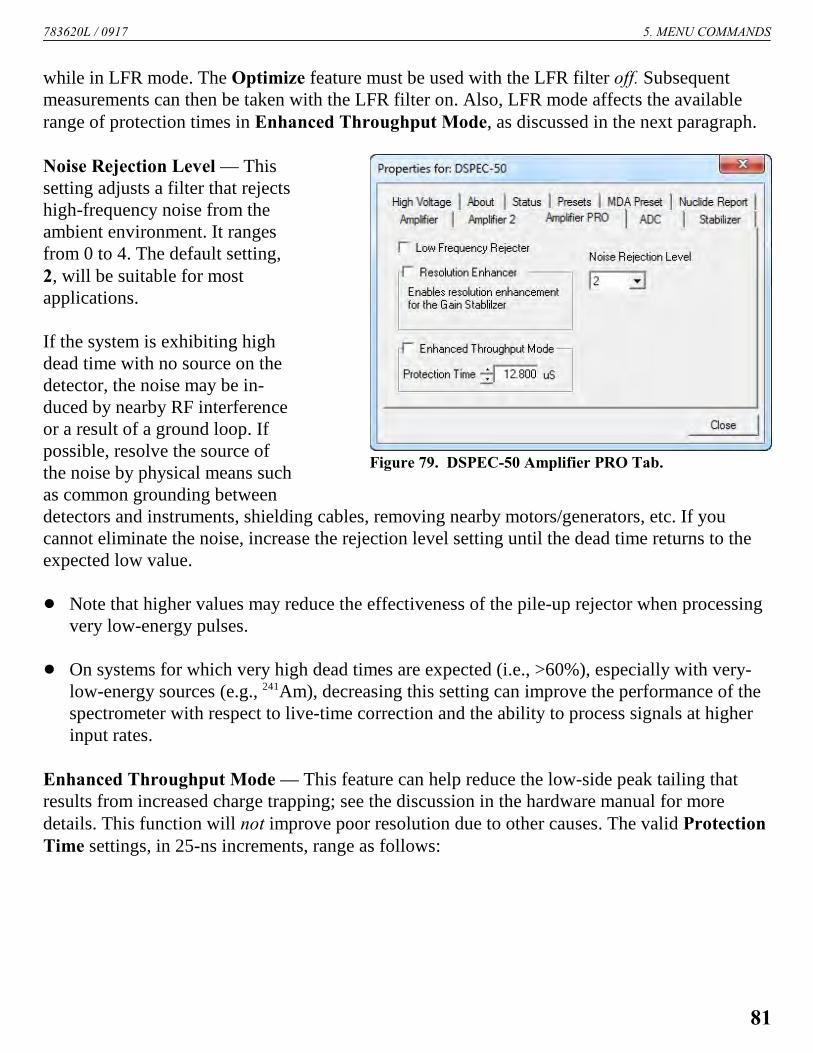
783620L / 0917 5. MENU COMMANDS
Figure 79. DSPEC-50 Amplifier PRO Tab.
while in LFR mode. The Optimize feature must be used with the LFR filter off. Subsequentmeasurements can then be taken with the LFR filter on. Also, LFR mode affects the availablerange of protection times in Enhanced Throughput Mode, as discussed in the next paragraph.
Noise Rejection Level — Thissetting adjusts a filter that rejectshigh-frequency noise from theambient environment. It rangesfrom 0 to 4. The default setting,2, will be suitable for mostapplications.
If the system is exhibiting highdead time with no source on thedetector, the noise may be in-duced by nearby RF interferenceor a result of a ground loop. Ifpossible, resolve the source ofthe noise by physical means suchas common grounding betweendetectors and instruments, shielding cables, removing nearby motors/generators, etc. If youcannot eliminate the noise, increase the rejection level setting until the dead time returns to theexpected low value.
! Note that higher values may reduce the effectiveness of the pile-up rejector when processingvery low-energy pulses.
! On systems for which very high dead times are expected (i.e., >60%), especially with very-low-energy sources (e.g., 241Am), decreasing this setting can improve the performance of thespectrometer with respect to live-time correction and the ability to process signals at higherinput rates.
Enhanced Throughput Mode — This feature can help reduce the low-side peak tailing thatresults from increased charge trapping; see the discussion in the hardware manual for moredetails. This function will not improve poor resolution due to other causes. The valid ProtectionTime settings, in 25-ns increments, range as follows:
81

GammaVision® V8 (A66-BW) 783620L / 0917
LFR Mode Highest Throughput(minimum Protection Time)
Lowest Throughput(maximum Protection Time)
Off (Rise Time + flattop) (2 × Rise Time + Flattop)
On (3 × Rise Time + 2 × Flattop) (6 × Rise Time + 3 × Flattop)
Turning on this feature automatically sets the minimum protection time (highest throughput rate)based on your current Rise Time and Flattop settings, however, you can adjust this value at anytime. Each time you change the rise time or flattop, the DSPEC-50 will automatically set itself tothe new minimum protection time.
“ Training” the Resolution Enhancer
The Resolution Enhancer operates by measuring the rise time (collection time) of the pulses andadjusting the gain based on the rise time. This is done on each pulse. The gain adjustment valuefor the rise time is stored in a table. The values in the table must be set by “training” the Resolu-tion Enhancer. Marking the Resolution Enhancer checkbox enables/disables the “learning”mode. Note that, once trained, the enhancer operates continuously until disabled as discussed inStep 13 below. To train the enhancer:
1) Set the bias, gain, rise time, flattop, and PZ as you would for data collection.
2) If you wish to use LFR Mode, turn it on.
3) If you wish to use Enhanced Throughput Mode, turn it on and either accept the automat-ically calculated, highest-throughput protection time, based on the current rise time and flat-top; or enter the desired setting. (The latter might require one or more data acquisitions.When finished, proceed to Step 4).
4) Clear the MCB and acquire a well-isolated peak.
5) Mark the Resolution Enhancer checkbox to turn on the learning mode.
6) You will now use the gain stabilization section of the Stabilizer tab to configure the Reso-lution Enhancer (the gain stabilizer is disabled in the learning mode). Enter the Centerchannel and Width of the peak acquired in Step 4; the maximum Width is 255 channels. Ifyou wish, use the Suggest button. The selected region should be as narrow as possible butshould completely include the peak.
7) Click on Initialize to clear all the Resolution Enhancer settings. Initialization does notchange the current Center channel and Width.
82

783620L / 0917 5. MENU COMMANDS
8) Clear the MCB, re-start acquisition, and monitor the FWHM of the target peak, using thePeak Info command (available by right-clicking in the spectrum window) to show theFWHM and peak counts. Collect about 5000 counts in the peak and record the FWHM.Clear the data and collect another 5000 counts, recording the FWHM. Repeat until theFWHM no longer changes. Typically, the more charge trapping exhibited by the detector,the longer the data collection time.
9) When you are satisfied that the FWHM has reached the best possible value, clear the MCBand collect another spectrum for confirmation.
10) At this point, the Resolution Enhancer is now “trained” for the current peak shape para-meters and the learning mode should be turned off by returning to the Amplifier PRO taband unmarking the Resolution Enhancer checkbox. The table of adjustments will be storedin the DSPEC-50's memory.
11) If you change any parameters that affect peak shape, you must repeat this “training”procedure.
12) Once the Resolution Enhancer has been trained and its checkbox has been unmarked, theStabilizer tab once again operates on the gain stabilizer (that is, it no longer adds values tothe table of adjustments).
NOTE The peak selected for the gain stabilizer can be different from the peak used fortraining the Resolution Enhancer.
13) To turn off the Resolution Enhancer, mark its checkbox to turn on the learning mode, go tothe Stabilizer tab and click on the Initialize button for the gain stabilizer. This will set theadjustment to zero. Now return to the Amplifier PRO tab and unmark the ResolutionEnhancer box.
ADC
This tab (Fig. 80) contains the Gate, ZDT Mode, Conversion Gain, Lower Level Discrim-inator, and Upper Level Discriminator controls. In addition, the current real time, live time, andcount rate are monitored at the bottom of the dialog.
Gate — This allows you to select a logic gating function. With this function Off, no gating isperformed (that is, all detector signals are processed); with the function in Coincidence, agating input signal must be present at the proper time for the conversion of the event; in Anti
83

GammaVision® V8 (A66-BW) 783620L / 0917
Figure 80. DSPEC-50 ADC Tab.
coincidence, the gating input signalmust not be present for the con-version of the detector signal. Thegating signal must occur prior toand extend 500 ns beyond peakdetect (peak maximum).
ZDT Mode — Use this droplist tochoose the ZDT Mode to be usedfor collecting the desired zero deadtime spectrum (see Section 5.2.11.4).The three modes are Off (LTC only),NORM_ CORR (LTC and ZDT),and CORR_ERR (ERR and ZDT).If one of the ZDT modes is selected,both spectra are stored in the samespectrum (.SPC) file. If you do not need the ZDT spectrum, you should select Off. In Gamma-Vision, the display can show either of the two spectra. Use <F3> or Acquire/ZDT DisplaySelect to toggle the display between the two spectra. In the Compare mode, <F3> switches bothspectra to the other type and <Shift+F3> switches only the compare spectrum. This allows youto make all types of comparisons.
Conversion Gain — This sets the maximum channel number in the spectrum. If set to 16384,the energy scale will be divided into 16384 channels. The conversion gain is entered in powersof 2 (e.g., 8192, 4096, 2048). The up/down arrow buttons step through the valid settings for theDSPEC-50.
Upper- and Lower-Level Discriminators — The Lower Level Discriminator sets the level ofthe lowest amplitude pulse that will be stored. This level establishes a lower-level cutoff bychannel number for ADC conversions. The Upper Level Discriminator sets the level of thehighest amplitude pulse that will be stored. This level establishes an upper-level cutoff by chan-nel number for storage.
Stabilizer
The DSPEC-50 has both gain and zero stabilizers (see Section ?). This tab (Fig. 81) shows thecurrent stabilizer settings. Each Adjustment section shows how much adjustment is currentlyapplied. The Initialize buttons reset the adjustment to 0. If the value approaches 90% or above,adjust the amplifier gain so the stabilizer can continue to function — when the adjustmentvalue reaches 100%, the stabilizer cannot make further corrections in that direction. TheCenter Channel and Width fields show the peak currently used for stabilization.
84
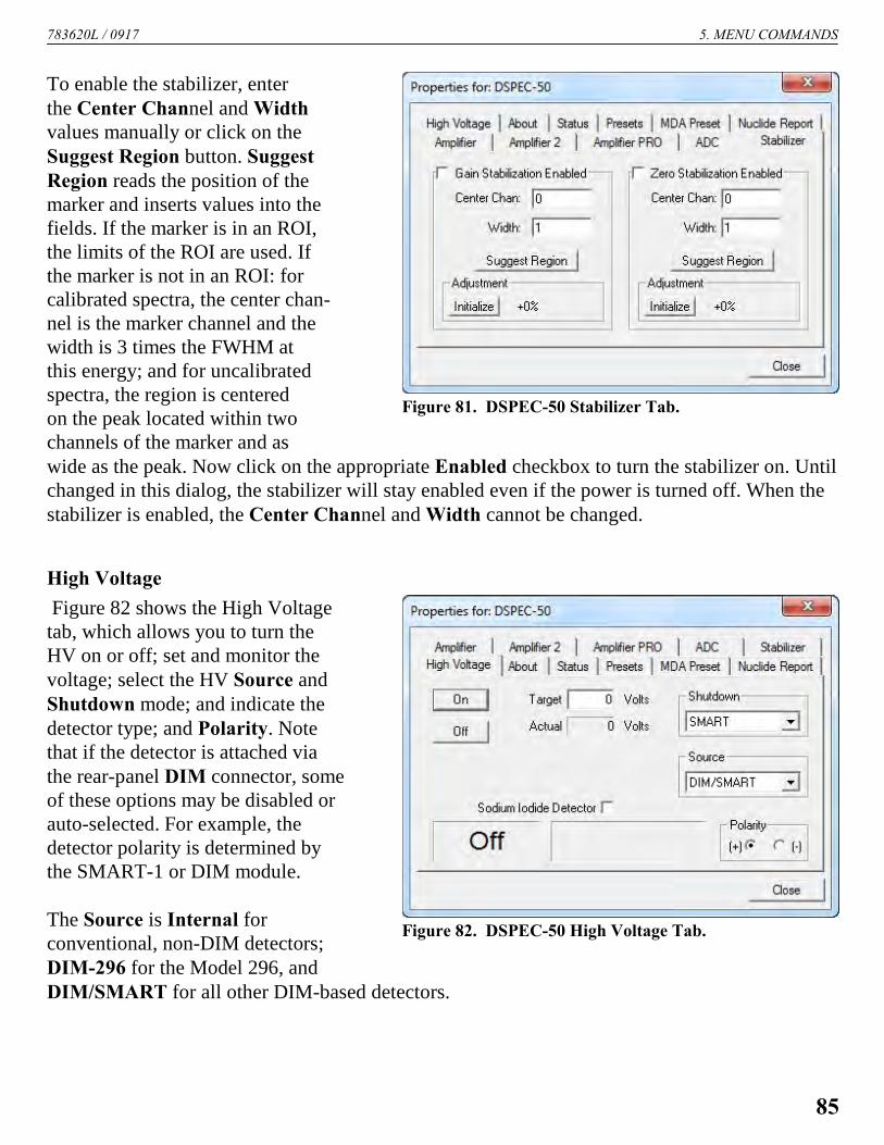
783620L / 0917 5. MENU COMMANDS
Figure 81. DSPEC-50 Stabilizer Tab.
Figure 82. DSPEC-50 High Voltage Tab.
To enable the stabilizer, enterthe Center Channel and Widthvalues manually or click on theSuggest Region button. SuggestRegion reads the position of themarker and inserts values into thefields. If the marker is in an ROI,the limits of the ROI are used. Ifthe marker is not in an ROI: forcalibrated spectra, the center chan-nel is the marker channel and thewidth is 3 times the FWHM atthis energy; and for uncalibratedspectra, the region is centeredon the peak located within twochannels of the marker and aswide as the peak. Now click on the appropriate Enabled checkbox to turn the stabilizer on. Untilchanged in this dialog, the stabilizer will stay enabled even if the power is turned off. When thestabilizer is enabled, the Center Channel and Width cannot be changed.
High Voltage
Figure 82 shows the High Voltagetab, which allows you to turn theHV on or off; set and monitor thevoltage; select the HV Source andShutdown mode; and indicate thedetector type; and Polarity. Notethat if the detector is attached viathe rear-panel DIM connector, someof these options may be disabled orauto-selected. For example, thedetector polarity is determined bythe SMART-1 or DIM module.
The Source is Internal forconventional, non-DIM detectors;DIM-296 for the Model 296, andDIM/SMART for all other DIM-based detectors.
85

GammaVision® V8 (A66-BW) 783620L / 0917
Figure 83. DSPEC-50 About Tab.
NOTE NaI detectors require the DIM-POSNAI interface and the DIM/SMART sourceselection.
Enter the Target high voltage, click On, and monitor the voltage in the Actual field. Click Offto turn off the high voltage.
The HV will not turn on if the detector is sending a remote shutdown or overload signal. TheOverload indicator means there is a bad connection in your system. The Shutdown indicatormeans that either the detector is warm or you have chosen the wrong Shutdown or Sourcemode.
The shutdown types are ORTEC, TTL, and SMART. The ORTEC mode is used for allORTEC detectors except SMART-1 (SMART) detectors. Most non-ORTEC detectors use theTTL mode; check with the manufacturer.
Choose the detector Polarity (SMART-1 detectors auto-select this setting). Normally, GEM(p-type) detectors have a positive signal and GMX (n-type) detectors have a negative signal.
To use a Sodium Iodide Detector, mark the checkbox. This changes the gain and zero stabili-zers to operate in a faster mode.
About
This tab (Fig. 83) displays hard-ware and firmware informationabout the currently selectedDSPEC-50 as well as the dataAcquisition Start Time andSample description. In addition,the Access field shows whetherthe Detector is currently lockedwith a password (Section 5.7.4),Read/Write indicates that theDetector is unlocked; ReadOnly means it is locked.
Status
Figure 84 shows the Status tab.You can select any six of these to be displayed simultaneously on the Status tab. The parametersyou choose can be changed at any time, so you can view them as needed. Two types of valuesare presented: OK or ERR, and numeric values. The SOH parameters return either OK or ERR.
86

783620L / 0917 5. MENU COMMANDS
Figure 84. DSPEC-50 Status Tab.
If the state is OK, the parameter stayed within the set limits during the spectrum acquisition.If the parameter varied from the nominal value by more than the allowed limit, the ERR is setuntil cleared by the program. The numeric values are displayed in the units reported by theDSPEC-50. Security, Detector temperature, and Live detector temperature are availableonly for SMART-1 detectors. For non-SMART-1 detectors, they display N/A.
Detector State of HealthReturns OK or an error mes-sage describing a problemwith detector power or bias.
+24 voltsThis is the current value ofthe +24 volt supply.
+12 voltsThis is the current value ofthe +12 volt supply.
!12 voltsThis is the current value ofthe !12 volt supply.
!24 voltsThis is the current value of the !24 volt supply.
High VoltageThis is the current value of the high voltage bias supply.
Note that, as of this release, the Detector temperature and Live detector temperaturemonitors are listed, but return only N/A.
Presets
Figure 85 shows the Presets tab. MDA presets are shown on a separate tab.
The presets can only be set on an MCB that is not acquiring data (during acquisition the presetfield backgrounds are inactive [gray]). You can use any or all of the presets at one time. To dis-able a preset, enter a value of zero. If you disable all of the presets, data acquisition will continueuntil manually stopped.
87
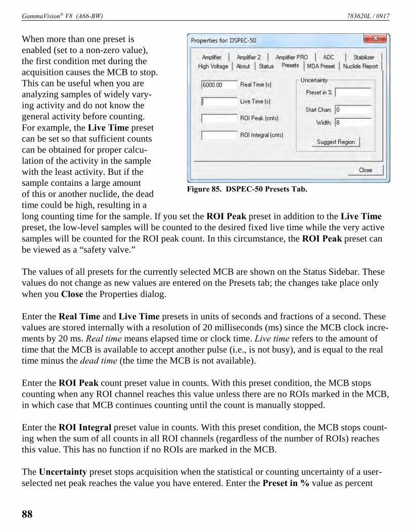
GammaVision® V8 (A66-BW) 783620L / 0917
Figure 85. DSPEC-50 Presets Tab.
When more than one preset isenabled (set to a non-zero value),the first condition met during theacquisition causes the MCB to stop.This can be useful when you areanalyzing samples of widely vary-ing activity and do not know thegeneral activity before counting.For example, the Live Time presetcan be set so that sufficient countscan be obtained for proper calcu-lation of the activity in the samplewith the least activity. But if thesample contains a large amountof this or another nuclide, the deadtime could be high, resulting in along counting time for the sample. If you set the ROI Peak preset in addition to the Live Timepreset, the low-level samples will be counted to the desired fixed live time while the very activesamples will be counted for the ROI peak count. In this circumstance, the ROI Peak preset canbe viewed as a “safety valve.”
The values of all presets for the currently selected MCB are shown on the Status Sidebar. Thesevalues do not change as new values are entered on the Presets tab; the changes take place onlywhen you Close the Properties dialog.
Enter the Real Time and Live Time presets in units of seconds and fractions of a second. Thesevalues are stored internally with a resolution of 20 milliseconds (ms) since the MCB clock incre-ments by 20 ms. Real time means elapsed time or clock time. Live time refers to the amount oftime that the MCB is available to accept another pulse (i.e., is not busy), and is equal to the realtime minus the dead time (the time the MCB is not available).
Enter the ROI Peak count preset value in counts. With this preset condition, the MCB stopscounting when any ROI channel reaches this value unless there are no ROIs marked in the MCB,in which case that MCB continues counting until the count is manually stopped.
Enter the ROI Integral preset value in counts. With this preset condition, the MCB stops count-ing when the sum of all counts in all ROI channels (regardless of the number of ROIs) reachesthis value. This has no function if no ROIs are marked in the MCB.
The Uncertainty preset stops acquisition when the statistical or counting uncertainty of a user-selected net peak reaches the value you have entered. Enter the Preset in % value as percent
88

783620L / 0917 5. MENU COMMANDS
uncertainty at 1 sigma of the net peak area. The range is from 99% to 0.1% in 0.1% steps. Youhave complete control over the selected peak region. The region must be at least 7 channels widewith 3 channels of background on each side of the peak. Note that GammaVision calculates thispreset once per 40 seconds. Therefore, the software will continue data acquisition up to40 seconds after the preset has been reached, and the uncertainty achieved for a high count-ratesample may be lower than the preset value.
Use the Start Channel and Width fields to enter the channel limits directly, or click on SuggestRegion. If the marker is positioned in an ROI around the peak of interest, Suggest Region readsthe limits of the ROI with the marker and display those limits in the Start Chan and Widthfields. The ROI can be cleared after the preset is entered without affecting the uncertainty calcu-lation. If the marker is not in positioned in an ROI: for calibrated spectra, the start channel is1.5 times the FWHM below the marker channel, and the width is 3 times the FWHM; for uncali-brated spectra, the region is centered on the peak located within two channels of the marker andas wide as the peak. The net peak area and statistical uncertainty are calculated in the samemanner as for the Peak Info command.
MDA Preset
The MDA preset (Fig. 86) can monitor up to 20 nuclides at one time, and stops data collectionwhen the values of the minimum detectable activity (MDA) for all of the user-specified MDAnuclides reach the needed value. Presets are expressed in Bq, and are evaluated every40 seconds. The detector must be calibrated for energy in all spectroscopy applications, and forefficiency in all applications but MAESTRO.
The MDA presets are implemented in the MCB (i.e., the entries you make on this screen aresaved in the MCB memory), and have no direct link to MDA methods selected in the analysisoptions for applications such as ScintiVision™, ISOTOPIC, etc. The MDA preset calculationuses the following formula:
where:a, b, and c are determined by the MDA criteria you choose.
Counts is the gross counts in an ROI that is 2.5×FWHM around the target peak energy.
Live time is evaluated in 40 second intervals for the MDA presets.
CorrectionFactor is the product of the calibration efficiency at the specified peak energy andthe peak’s branching ratio (yield) as listed in the working (active) library.
89

GammaVision® V8 (A66-BW) 783620L / 0917
Figure 86. DSPEC-50 MDA Preset Tab.
To add an MDA preset, enter thepreset value in the MDA or Corre-ction field; select the Nuclide andEnergy; enter the desired valuesfor coefficients a, b, and c; thenclick Add New.
To edit an existing preset, click tohighlight it in the table. This willload its Nuclide, Energy, and coef-ficients in the lower sections of thedialog. Change as needed, thenclick Update.
To remove a preset, click to high-light it in the table, then click Delete.
IMPORTANT These MDA presets are not dynamically calculated. Each time you add anMDA preset to this table, its CorrectionFactor value is calculated and stored inthe MCB’s memory. If you then load a different library, change the efficiencycalibration, or change the system geometry, the spectroscopy application willnot update the existing CorrectionFactors, and your MDA presets may nolonger be applicable.
Nuclide Report Tab
Figure 87 shows the Nuclide Report tab. The Nuclide Report displays the activity of up to nine(9) user-selected peaks. Once the report is set up, the two lowest-energy ROIs and their respec-tive activity readouts are displayed on the DSPEC-50's Spectrum screen.
The peak area calculations in the hardware use the same methods as the Peak Info calculation(Section 5.4.3) so the Nuclide Report display is the same as the Peak Info display on the selec-ted peak in the spectra stored in the computer. The calculated value is computed by multiplyingthe net peak count rate by a user-defined constant. If the constant includes the efficiency andbranching ratio, the displayed value is the activity. You enter the nuclide label and the activityunits. The report format and calculations are discussed in the next section.
IMPORTANT The entries you make on this screen are saved in the MCB memory, and are notdynamically calculated. If you change the energy calibration (i.e., if the peaklocations shift), the Nuclide Report may no longer be valid.
90

783620L / 0917 5. MENU COMMANDS
Figure 87. Nuclide Report Tab.
Add New
You can add Nuclide Peaks to thereport manually or by selectingthe peaks from the current work-ing library. The spectrum mustbe energy calibrated to use thelibrary method.
! Defining Peaks Manually— To manually define peaks,enter the Nuclide name, ROILow (start) and High (end)channels, multiplicative Fac-tor and Units in the Reportsection; then click Add New.All nuclides in the table usethe same units, so that value need only be entered once.
! Selecting Peaks from the Working Library — To define report peaks using the library,select the Nuclide and gamma-ray Energy in the Library section. This defines whichgamma ray to use. Now, in the Report section, click the Select from Lib button. Enter theFactor and Units, then click Add New to add this nuclide to the list. The ROI for thispeak will be marked in the MCB’s spectrum window, centered on the peak energy and3 times the width of the calibrated FWHM.
Edit
To change any of the current nuclides, select the nuclide in the list (use the scroll bars if needed).This will show the current settings for this nuclide. Make any changes needed. Any or all of theentries can be changed. When finished with the changes, click on Update.
Delete
To remove an entry, select the entry and click Delete.
When you close the Properties dialog, all the values entered are written to the DSPEC-50 and thetwo lowest-energy ROIs and corresponding activity readouts are displayed on the DSPEC-50screen.
91

GammaVision® V8 (A66-BW) 783620L / 0917
5.2.11.2. Nuclide Report Calculations
The Nuclide Report displays the activity of up to 9 user-selected peaks. Once the report is set upyou can view the Nuclide Report at any time. The peak area calculations are the same as thecalculations in GammaVision and other ORTEC software, so the Report contents can be dupli-cated using the spectra stored in the computer. The calculated value is computed by multiplyingthe net peak count rate by a user-defined constant. If the constant includes the efficiency andbranching ratio, the displayed value will be activity. The nuclide label and the activity units areentered by the user.
The report has this format:
Nuclide keV uCi/m2 ±%
CO-60 1332.5 1.21E+01 10.2
CO-60 1173.2 1.09E+01 12.3
CO-57 122.1 1.48E+00 86.2
Calculations
These are the calculations used to generate the Nuclide Report’s Activity, Uncertainty, andPeak values.
Activity is calculated as follows:
NucCoef is normally the inverse of efficiency times the branching ratio. Note that theefficiency is the ABSOLUTE counting efficiency for the source/detector geometry beingused. Thus, in order to get meaningful activity results, as in any counting situation, you needto have efficiency factors which are appropriate to the actual counting geometry. If NucCoefis set to 1, you will get peak count rate on the display.
LiveTime is the current live time.
NetCounts is computed with the following equation:
92

783620L / 0917 5. MENU COMMANDS
GrossCounts is the sum of the counts in the ROI, excluding the first and last 3 channels ofthe ROI.
Background is:
ROIWidth is:
Uncertainty (in percent) is calculated as follows:
Peak is the position of the maximum count and is computed with the following equation:
MaximumROIChan is the channel in the ROI with the most counts. If there are no data, thecenter channel of the ROI is used.
EnergySlope and EnergyIntercept are the energy calibration values as entered by keypad (ondigiDARTs) or by software. If the values are not present, the result is given in channels.
5.2.11.3. Gain and Zero Stabilization
The gain stabilizer requires a peak in the spectrum to monitor the changes in the gain of thesystem amplifier. The gain stabilizer controls the amplification factor of a separate amplifier sothat the peak will be maintained in its original position.
The zero stabilizer enables you to control the zero-level (or offset) stabilizer. The zero-levelstabilizer uses a peak in the spectrum to monitor the changes in the zero level of the system
93

GammaVision® V8 (A66-BW) 783620L / 0917
amplifier. The zero stabilizer controls the offset bias level so the peak will be maintained in itsoriginal position.
For both functions, the input pulse-height-to-channel-number relationship is:
where:Intercept = The channel number of the zero-height input pulseGain = The relation between pulse height and channel number (slope of the curve)
Changes in either the intercept or gain can affect the positions of all the peaks in the spectrum.When used with the zero stabilizer, both the zero intercept and the gain (slope) will be monitoredto keep all the peaks in the spectrum stabilized. The zero stabilization and gain stabilization areseparate functions but both will affect the position of the peaks in the spectrum.
The stabilization operates by keeping a peak centered in an ROI you have defined. The ROIshould be made symmetrically about the center of a peak with reasonably good count rate in thehigher channels of the spectrum. The ROI should be about twice the FWHM of the peak. If theregion is too large, counts not in the peak will have an effect on the stabilization.
Before setting either stabilization peak, the coarse and fine gains should be set to the desiredvalues, and optimization or pole-zero performed.
5.2.11.4. ZDT (Zero Dead Time) Mode
An extended live-time clock increases the collection time (real time) of the acquisition to correctfor input pulse train losses incurred during acquisition due to system dead time. This correctedtime value, known as the live time, is then used to determine the net peak count rates necessaryto determine nuclide activities.
As an example, consider the case where the spectrometry amplifier and ADC are 60% deadduring the acquisition. The elapsed real time will be:
94

783620L / 0917 5. MENU COMMANDS
If the N counts in the gamma-ray peak in the spectrum are divided by the elapsed live time, theresulting counting rate, is now corrected for dead-time losses. The standard
deviation in that counting rate is .
Unfortunately, extending the counting time to make up for losses due to system-busy results inan incorrect result if the gamma-ray flux is changing as a function of time. If an isotope with avery short half-life is placed in front of the detector, the spectrometer might start out with a veryhigh dead time, but the isotope will decay during the count and the dead time will be zero by theend of the count. If the spectrometer extends the counting time to make up for the lost counts, itwill no longer be counting the same source as when the losses occurred. As a result, the numberof counts in the peak will not be correct.
When a supported ORTEC MCB operates in ZDT18 mode, it adjusts for the dead-time losses bytaking very short acquisitions and applying a correction in real time — that is, as the data arecoming in — to the number of counts in the spectrum. This technique allows the gamma-ray fluxto change while the acquisition is in progress, yet the total counts recorded in each of the peaksare correct. The resulting spectrum has no dead time at all — in ZDT mode, the data are correc-ted, not the acquisition time. Thus, the net counts in a peak are divided by the real time todetermine the count rate.
ZDT mode has a unique feature in that it can store both the corrected spectrum and the uncor-rected spectrum, or the corrected spectrum and the uncertainty spectrum. Therefore, supportedMCBs allow you to choose between three ZDT Mode settings on the ADC tab under MCBProperties...: Off, NORM_CORR, and CORR_ERR.
! Off — Uncorrected Spectrum OnlyIn this mode, only the uncorrected spectrum (live time and real time with dead-time losses)— also called the live-time-corrected or LTC spectrum — is collected and stored in the .SPC
file. The LTC spectrum can be used to determine exactly how many pulses at any energywere processed by the spectrometer. The corrected spectrum gives the best estimate of thetotal counts that would have been in the peak if the system were free of dead-time effects.The uncertainty spectrum can be used to calculate the counting uncertainty, channel by
18U.S. Patent 6,327,549.
95

GammaVision® V8 (A66-BW) 783620L / 0917
channel, in the corrected spectrum.
NOTE When the spectrometer is placed in ZDT mode, the throughput of the instrument isreduced somewhat as extra processing must be done on the spectrum; therefore, ifthe gamma-ray flux is not changing as a function of time, but absolute highestthroughput is desirable, you may wish to store only the LTC spectrum in the MCBmemory.
! NORM_CORR — ZDT and Uncorrected Spectra StoredWhen the ZDT mode is set to NORM_CORR, the two spectra stored are the LTC spectrumand the ZDT spectrum (corrected for the dead-time losses; real time only). Unfortunately, inthe analysis of the ZDT spectrum, the uncertainty of the measurement cannot be determinedusing either spectrum.
NOTE This mode is not useful for quantitative analysis if the counting rate varies signifi-cantly during the measurement time, particularly if the user desires an accuratecounting rate and standard deviation calculation. When you select the NORM_CORR mode, GammaVision ignores the ZDT spectrum and analyzes the LTCspectrum as it would for the Off ZDT mode.
! CORR_ERR — ZDT and Error Spectra StoredIn the CORR_ERR mode, the estimation of the statistical uncertainty is stored in place ofthe LTC spectrum, and is referred to as the error spectrum (ERR). In this mode, the ZDTspectrum is used to measure the counts in a peak, and the error spectrum is used to determinethe uncertainty of the measurement made in the corrected spectrum.
For example, if the area of a peak is measured in the corrected spectrum by summing chan-nels 1000 to 1100, the variance of the measurement can be determined by summing thecounts in channels 1000 to 1100 in the error spectrum. Or, shown another way, the counts in
channel i can be expressed as ± with a 1-sigma confidence limit, where N is the
corrected spectral data and V is the variance (error) spectral data.
The live time is set to the real time within the analysis engine during the analysis of ZDTspectra.
Table 1 shows which spectra are collected in the three possible ZDT modes.
96

783620L / 0917 5. MENU COMMANDS
Mode UncorrectedSpectrum
ZDT CorrectedSpectrum
ZDT ErrorSpectrum
Off (ZDT Disabled) Yes No No
NORM_CORR (ZDT–LTC Mode) Yes Yes No
CORR_ERR (ZDT–ERR Mode) No Yes Yes
Table 1. ZDT Modes.
Choosing a ZDT Mode
When the counting rate is essentially constant during the time required to acquire the spectrum,the standard mode — ZDT Off — is the preferred mode; only the uncorrected spectrum is col-lected and stored in the spectrum file. But, if the counting rate varies significantly during themeasurement time, the standard mode will not yield the proper dead-time-corrected countingrate. This can be most easily understood by noting that the uncorrected mode compensates fordead-time losses by extending the real counting time. Hence a sample containing both a short-lived high-activity isotope and a long-lifetime lower-activity isotope will experience very highdead-time losses during the first few seconds of the measurement, as the short-lifetime isotopedecays rapidly. This high dead time will cause the counting time to be extended after the short-lived isotope has decayed to zero activity, and the system will count the low-activity isotopefor the extra time. Consequently, the average activity of the short-lived isotope will be under-estimated.
If you anticipate significantly varying counting rates during the time taken to acquire the spec-trum, the CORR_ERR ZDT mode should be used. The CORR_ERR mode corrects for dead-time losses over minuscule time intervals by adding counts to the ZDT spectrum in proportion tothe instantaneous ratio of real time to live time. Thus, the dead-time correction can correctlytrack rapidly changing counting rates. The CORR_ERR mode should be used whenever thecounting rate may change significantly during the measurement time. In addition to the rapidlydecaying isotope example above, the CORR_ERR mode should be used when monitoring cool-ing water flow from a nuclear reactor. The CORR_ERR mode accommodates brief bursts ofhigh-activity in the water flowing past the gamma-ray detector. Both the corrected and errorspectra are stored in the resulting spectrum file.
Note that the counts in the ZDT spectrum must be divided by the elapsed REAL time to computethe dead-time corrected counting rate. It is important to note that the standard deviation in the
NZDT counts in a gamma-ray peak in the ZDT spectrum is not . Instead the standard devia-
tion is obtained from the NERR counts in the same peak ROI in the accompanying error spectrum.
97
GammaVision® V8 (A66-BW) 783620L / 0917
The standard deviation in this case is . And the standard deviation in the computed count-
ing rate, , is .
The NORM_CORR Diagnostic Mode
Why is there a NORM_CORR mode, and why should you avoid using it? This mode simul-taneously collects the ZDT spectrum and the conventional uncorrected spectrum. It is useful fordemonstrating that the counts in the uncorrected spectrum divided by the live time is the samecounting rate as the counts in the ZDT spectrum divided by the real time, in the special case ofconstant counting rate. Because the error spectrum is not collected in NORM_CORR mode, thestandard deviation in the ZDT counts cannot be calculated if the counting rate is varying.
GammaVision provides some protection for users if the ZDT-LTC mode is inadvertentlyselected. In this case, GammaVision ignores the ZDT spectrum and presumes you intended touse the uncorrected spectrum in a constant-counting-rate application.
To summarize:
! Use the ZDT Off mode when the counting rate is expected to be constant during the timetaken to acquire the spectrum.
! Use the ZDT CORR_ERR mode when the counting rate is expected to change or mightchange significantly during the time required to acquire the spectrum.
! Avoid using the NORM_CORR mode because GammaVision V8 will default to analyzingthe LTC spectrum and will ignore the ZDT spectrum.
More Information
Visit our website or contact your ORTEC representative for more detailed information:
! Application note AN56, “Loss Free Counting with Uncertainty Analysis Using ORTEC’sInnovative Zero Dead Time Technique,” (http://www.ortec-online.com/pdf/an56.pdf)
! General gamma spectroscopy technical papers (http://www.ortec-online.com/papers/
reprints.htm#General)
5.2.11.5. InSight Mode
The InSight display (Fig. 88) shows the actual sampled waveform in the digital processing unitson a reference graticule. The Properties dialog remains active and can be used to change settings
98

783620L / 0917 5. MENU COMMANDS
Figure 88. The InSight Mode Display.
while viewing the pulses. As none of the traditional analog signals are available in digitalMCBs, this mode is the only way to display the equivalent amplifier output pulse. Note that atthe bottom of the window the marker channel is displayed in units of time.
To exit the InSight mode and return to the PHA display, press <Esc> or go to the Insight sectionon the Amplifier 2 tab and click on Stop. The PHA mode is set to STOP when in the InSightmode.
InSight Mode Controls
The Status Sidebar changes from the PHA mode controls to the InSight controls for adjusting thepeak display (Fig. 88) On the left is a vertical scrollbar for adjusting the vertical offset of thewaveform. The value of the offset is shown on the display. Double-clicking the mouse in the scrollbar will set the vertical offset to the vertical value of the channel at the marker position.
99
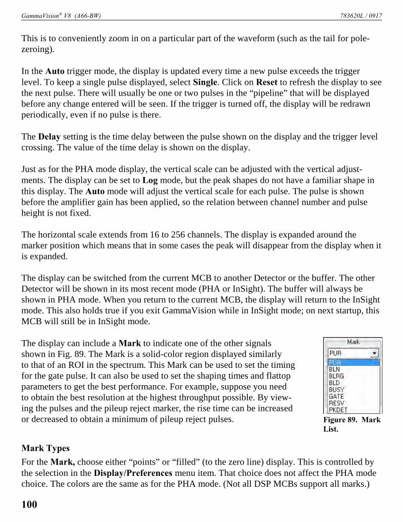
GammaVision® V8 (A66-BW) 783620L / 0917
Figure 89. MarkList.
This is to conveniently zoom in on a particular part of the waveform (such as the tail for pole-zeroing).
In the Auto trigger mode, the display is updated every time a new pulse exceeds the triggerlevel. To keep a single pulse displayed, select Single. Click on Reset to refresh the display to seethe next pulse. There will usually be one or two pulses in the “pipeline” that will be displayedbefore any change entered will be seen. If the trigger is turned off, the display will be redrawnperiodically, even if no pulse is there.
The Delay setting is the time delay between the pulse shown on the display and the trigger levelcrossing. The value of the time delay is shown on the display.
Just as for the PHA mode display, the vertical scale can be adjusted with the vertical adjust-ments. The display can be set to Log mode, but the peak shapes do not have a familiar shape inthis display. The Auto mode will adjust the vertical scale for each pulse. The pulse is shownbefore the amplifier gain has been applied, so the relation between channel number and pulseheight is not fixed.
The horizontal scale extends from 16 to 256 channels. The display is expanded around themarker position which means that in some cases the peak will disappear from the display when itis expanded.
The display can be switched from the current MCB to another Detector or the buffer. The otherDetector will be shown in its most recent mode (PHA or InSight). The buffer will always beshown in PHA mode. When you return to the current MCB, the display will return to the InSightmode. This also holds true if you exit GammaVision while in InSight mode; on next startup, thisMCB will still be in InSight mode.
The display can include a Mark to indicate one of the other signalsshown in Fig. 89. The Mark is a solid-color region displayed similarlyto that of an ROI in the spectrum. This Mark can be used to set the timingfor the gate pulse. It can also be used to set the shaping times and flattopparameters to get the best performance. For example, suppose you needto obtain the best resolution at the highest throughput possible. By view-ing the pulses and the pileup reject marker, the rise time can be increasedor decreased to obtain a minimum of pileup reject pulses.
Mark Types
For the Mark, choose either “points” or “filled” (to the zero line) display. This is controlled bythe selection in the Display/Preferences menu item. That choice does not affect the PHA modechoice. The colors are the same as for the PHA mode. (Not all DSP MCBs support all marks.)
100
783620L / 0917 5. MENU COMMANDS
None No channels are marked in the display.
PUR The region marked indicates when the PUR circuit has detected pileup and isrejecting the marked pulses.
BLN This shows when the negative baseline discriminator has been triggered. Typi-cally this signal only marks the TRP reset pulse. The signal is used internally inthe live-time correction, baseline restoration, and pile-up rejection circuits.
BLRG This shows when the baseline restorer is actively restoring the baseline.
BLD This shows when the positive baseline discriminator has been triggered. Thesignal is used internally in the live-time correction, baseline restoration, and pile-up rejection circuits.
BUSY When the busy signal is active, Busy shows in the Mark box. It represents thedead time.
GATE This shows when the gate signal is present on the gate input connector. If theGate mode on the ADC tab (see Fig. 88) is set to Off, then all regions aremarked. If the mode is set to Coincidence, then the marked region must overlapthe pulse peak (that is, must start before the beginning of the flattop and stop afterthe end of the flattop) for the pulse to be counted. If the mode is set to Anticoin-cidence, then the marked region will show the pulses that are accepted. That is,the rejected peaks will not be marked. Simply put, in all modes the acceptedpeaks are marked.
RESV Reserved.
PKDET This is the peak detect pulse. It indicates when the peak detect circuit has detec-ted a valid pulse. The Mark occurs about 1.5 ìs after the pulse maximum on thedisplay.
On the lower right of the InSight display are the shaping parameter controls. The controls aresplit into two groups, and the other controls... button switches between them. (Not all DSPMCBs support all of the controls.)
One group includes Rise Time, Flattop, Tilt, and the Optimize button. The Rise Time value isfor both the rise and fall times; thus, changing the rise time has the effect of spreading ornarrowing the quasi-trapezoid symmetrically.
101

GammaVision® V8 (A66-BW) 783620L / 0917
Figure 90. An Example of the Tradeoff BetweenThroughput and Count Rate.
The Flattop controls adjust the top of the quasi-trapezoid. The Width adjusts the extent of theflattop (from 0.3 to 2.4 ìs). The Tilt adjustment varies the “flatness” of this section slightly. TheTilt can be positive or negative. Choosing a positive value results in a flattop that slopes down-ward; choosing a negative value gives an upward slope. Alternatively, Optimize can set the tiltvalue automatically. This value is normally the best for resolution, but it can be changed on thisdialog and in the InSight mode to accommodate particular throughput/resolution tradeoffs. TheOptimize button also automatically adjusts the pole-zero setting.
5.2.11.6. Setting the Rise Time in Digital MCBs
To achieve the best results for your application, when using a digital spectrometer, such as aDSPEC-series instrument, we recommend that you set the rise time of the pulses being processedby the digital filter to the minimum value for the resolution needed.
The pulse rise time (and also fall time) is based on the time required for each pulse to reach itspeak value. This “peaking time” is about twice that indicated by the conventional time constantsdisplayed on the front panel of commercial analog amplifiers. For example, germanium detectorsare often specified at a 6-ìs time constant; this setting is equivalent to 12-ìs peaking (rise) timein our digital spectrometers.
Up to some value of rise time, onecan expect improved resolution withincreasing rise time; there will, how-ever, be a tradeoff in maximumthroughput to memory. Figure 90illustrates an example of this tradeoff.ORTEC digital spectrometers operatewell above the peak of the throughputcurve. Operating there allows theseinstruments to handle an even higherrate of incoming counts, but with lessdata into memory and, therefore, alonger count time to the same detectionlimit. It is possible to move the peak of the curveto the right (more counts to memory with higherinput count rate) by reducing the pulse rise (andfall) time, thereby trading off resolution formaximum count rate.
Table 2 is a guide to choosing a countrate that will ensure that the most efficientoperation of your digital spectrometer over
Input Count RateDynamic Range
MaximumThroughput
Rise Time(ìs)
0--->20000 9000 12
0--->50000 12500 8
0--->75000 23500 4
0--->100000 37000 2.4
0--->150000 50000 1.6
0--->200k 70000 0.8
0--->220k 85000 0.6
0--->250k 100000 0.4
0--->300k 120000 0.2
Table 2. Rise Time Selection Guide.
102

783620L / 0917 5. MENU COMMANDS
Figure 91. CalibrationMenu.
the range of anticipated input count rates for your application — that is, at or belowthe throughput peak — while achieving the best resolution obtainable from the detectorconsistent with that requirement. Enter the rise time that best matches your dynamic range ofcount rate (note that the available rise-time settings will vary by instrument; this chart is ageneral guide only).
The longest rise time shown in the table is 12 ìs, even though some digital instruments can beset for rise times as long as 23 ìs. If throughput is not an issue because all samples are low rate,increasing the rise time beyond 12 ìs might achieve a small improvement in resolution. Forplanar detectors, such as ORTEC’s GLP, Si(Li), IGLET, and IGLET-X Series, operating atlonger rise times frequently gives improved resolution.
5.3. Calibrate
Figure 91 shows the Calibrate menu. GammaVision’s calibra-tion features include a Calibration Wizard to simplify the energy and efficiency calibrations as well as a fully implemented true-coincidence correction (TCC) calibration. This menu also allows you toaccess the energy and efficiency calibration features directly from themenu rather than stepping through the wizard.
The energy and efficiency calibrations of the spectrum in theDetector, and the calibration wizard are only available if theDetector is not acquiring data. If there is no energy calibration,then all choices except Energy..., Recall Calibration..., andCalibration Wizard... are inactive (gray). If the efficiency calibration exists, there will be acheckmark by the menu item.
5.3.1. General Information, Cautions, and Tips
The calibration of the system defines four relations:
! Spectrum channel numbers and energy! FWHM of the peak and energy! Spectrum count rate and activity in becquerels or other units! True coincidence summing factor and energy
The data collected are in counts/unit time/channel; however, to be most useful, these data needto be converted to activities (i.e., decays/unit time at a given energy). The calibration parametersdo this conversion.
These relationships are calculated from spectra, user inputs, and inputs from libraries and tables.
103

GammaVision® V8 (A66-BW) 783620L / 0917
The calibration data are merged with the spectrum when it is saved as an .SPC file. The informa-tion is used in the analysis section to perform the desired analysis. Spectra saved in the .CHN
format are compatible with older software, however the .CHN format does not contain theefficiency or TCC calibration data.
The energy calibration and the efficiency calibration are separated to make it easier to do thesecalibrations. The efficiency and TCC calibrations are linked because the TCC depends on thedetector/source geometry. If properly chosen sources and libraries are used, the calibration pro-cess is simple, quick and accurate. The input values can be saved so that repeated calibrationswith the same source are easy and simple.
The energy calibration can be changed without affecting the efficiency calibration. By using theRecall Calibration... command, the previously calculated efficiency calibration can be insertedinto the new calibration data.
5.3.1.1. For Best Calibration Results
It is important that the energy, efficiency, and TCC calibrations be done correctly because thecalibration results will affect all analyses employing them. The energy calibration data is used todefine the energies of the peaks in the spectrum. If incorrect, the calculated energies will not cor-respond to the correct library entry and the peak might be incorrectly identified. The shape para-meters are used to define the expected shape for a singlet peak. If incorrect, peaks will be labeledas having a bad shape when they do not, and bad peaks will not be marked. Peaks marked withpoor shape might not be included in the activity calculation, resulting in loss of accuracy evenfor singlet peaks. For deconvolutions, these parameters define the Gaussian shape used for thecomponents of the total peak area. Incorrect peak shapes can result in poor deconvolution resultsand even incorrect peak height ratios in multiplets.
An incorrect efficiency calibration can cause the nuclide activity to be incorrectly reported. Theknee value, if incorrectly chosen, can cause poor results near the knee, especially below theknee.
Using many data points near the knee aids in selecting the correct knee energy. A poor choice oftype of fit can result in a good fit to poor data, which will yield a poor efficiency calibration.
NOTES During efficiency calibration, the net peak area calculation can be affected by thelibrary Match Width setting in effect at the time the calibration is performed. Beforestarting an efficiency calibration, go to the System tab under Analyze/Settings/Sample Type... (page 152) and make sure the Match Width is set to the same valueyou will be using during analysis. Most users will keep the default setting, 0.5. Ifusing a different setting, we recommend a value between 0.4 and 0.75.
104
783620L / 0917 5. MENU COMMANDS
(8)
(9)
(10)
For TCC calibrations, the library and TCC table should include only the nuclides pre-sent in the spectrum. In addition, note that when recalling the TCC calibration from aFile in the Calibration Wizard, the TCC efficiency calibration from the same file mustalso be recalled; otherwise, the TCC calibration loaded may not be complete and willnot produce accurate results.
5.3.2. Energy...
5.3.2.1. Introduction
The Energy... calibration function calculates two sets of parameters: the energy vs. channelnumber, and the peak shape or FWHM vs. energy. The inputs to this function are a spectrum orseries of spectra with isolated peaks distributed over the energy range of interest, and either alibrary or table of peak energies. The library referred to here is an analysis gamma-ray library.The creation of a table of peak energies is described in this section.
The formula for energy vs. channel number is:
where:E = energyai = coefficientsC = channel number
The formula for FWHM vs. channels is:
where:F = FWHM in channelsbi = coefficientsC = channel number
To calculate the FWHM in energy use the following:
where:F(e) = FWHM in energy
105

GammaVision® V8 (A66-BW) 783620L / 0917
Figure 92. Energy Calibration Sidebar.
F(c) = FWHM in channels at channel Ca2 = energy calibration slope defined in Eq. 8a3 = energy calibration quadratic coefficient defined in Eq. 8C = channel number
When the FWHM fit is made, the fit is automatically checked for validity. If the FWHM curve isnegative at any part of the spectrum or the curve bends over (has a maximum and then goesdown), a warning message, Non-physical FWHM fit, is displayed. Click OK, then display theFWHM curve to see why the fit is incorrect. Also, if the delta between the data points and theFWHM fit is greater than 25%, a message is displayed. The curve can be accepted if the warningis due to the fit outside the energy of interest, or some of the data points might need to bedeleted. The calibration spectrum should have good peaks with many counts, so counting longermight remedy the poor fit.
The same methods used to calculate the peak centroid and width in the Calibrate section areused in the Analyze section. This ensures consistency of results.
The energy calibration is done using the spec-trum in the buffer or the Detector. The calibra-tion is linked to the spectrum used and is trans-ferred with it when the spectrum is transferred(e.g., from Detector to buffer or disk file).
The first step in the calibration is to collect aspectrum of a known source with isolated peaks.The spectrum peaks must be well-defined witha small statistical uncertainty. When the Detec-tor has finished collection (i.e., stopped), selectCalibrate from the menu bar, then Energy....The Energy Calibration Sidebar (Fig. 92) willautomatically open. The Calibration Sidebar can be moved by its title bar to another position.It is usually helpful to zoom in on the spectrum so the peaks are clearly displayed.
5.3.2.2. Auto Calibration19
The Auto Calibrate button will perform a complete energy and FWHM calibration on thedisplayed spectrum using the working library. This automatic calibration is suitable only forHPGe spectra and requires at least three peaks (five preferred) in the spectrum that are in thelibrary. There can be a different number of peaks in the spectrum than in the library, that is, therecan be peaks in the spectrum that are not in the library and peaks in the library that are not in the
19U.S. Patent 6,006,162.
106

783620L / 0917 5. MENU COMMANDS
spectrum. The spectrum can be uncalibrated, calibrated, or even incorrectly calibrated. Spectrasuch as the mixed gamma standard or uranium ore can be used with the appropriate library.
Auto Calibrate works as follows: the spectrum is searched for all the major peaks, then thispeak list is compared to the library peak list to find the calibration that gives the best match.
NOTE If the No FWHM Cal checkbox on the Energy Calibration sidebar is marked, theFWHM calibration is not changed during calibration. This might be desirable whendecay of short-lived isotopes in a calibration source results in peaks that are adequatefor an energy calibration but whose shape might not be optimal for the FWHMcalibration.
5.3.2.3. Manual Calibration
NOTELow Resolution systems (i.e., NaI, LaBr, CsI, etc.) must be calibrated for Energy
and FWHM using this Manual Calibration method, and each peak used in thecalibration should be marked with a Region of Interest (ROI) that fully covers theentire peak including the background channels.
If there is no energy calibration, the energy of one or two known peaks must be entered. Usingthe Full Spectrum View, select a peak in the high energy (channel) part of the spectrum. Whenthis part of the spectrum is visible in the expanded display, move the cursor to the known peak. For Low Resolution systems an ROI must be marked around the peak. At this time the centroidof the peak will be calculated and displayed in the upper part of the Energy Calibration Sidebaras, in this example, Channel: 11342.66. This is the channel number of the peak centroid. Nowclick in the E= input box and enter the energy of this peak. Click the Enter button or press<Enter>. A table and graph will appear on the screen (Fig. 93). They can be moved around andsized if they obscure the spectrum.
The table shows one value (the one just entered), and the graph shows a straight line fit from(energy = 0, channel = 0) to the energy and channel just entered. This is an approximate calibra-tion; it should be fairly accurate if the zero offset is small.
The Energy and FWHM radio buttons at the bottom of the Energy Calibration Sidebar displaythe table and graph for either energy vs. channel (Fig. 93) or FWHM vs. energy (Fig. 94).
Click FWHM. The table shows the one value entered and the graph shows a horizontal line. Fora single point, the FWHM is assumed to be a constant.
Using the Full Spectrum View (or the Library List window), select a peak in the low-energy partof the spectrum and move the marker to the centroid of the peak. For Low Resolution systemsan ROI must be marked around the peak. Again click in the E= field at the top of the sidebar
107

GammaVision® V8 (A66-BW) 783620L / 0917
Figure 93. Energy Calibration Display.
and enter the energy of this peak. Both the energy function and FWHM function, as well as theircorresponding tables, will update with the new entry so progress can be monitored.
At this time, the cursor can be positioned using the calibration graphs, calibration table, FullSpectrum View, or Expanded Spectrum View. The cursor will show the energy based on thecalibration up to this point.
The calibration can be refined by adding as many points as desired. For Low Resolution systemsan ROI must be marked around each peak. Any point can be deleted by selecting that point inthe table of values (Energy or FWHM) and clicking on the Delete Energy button on thecalibration sidebar. The fit updates when a point is removed.
NOTE If the No FWHM Cal checkbox on the Energy Calibration sidebar is marked, the
108

783620L / 0917 5. MENU COMMANDS
Figure 94. FWHM Calibration Display.
FWHM calibration is not changed during calibration. This might be desirable whendecay of short-lived isotopes in a calibration source results in peaks that are adequatefor an energy calibration but whose shape might not be optimal for the FWHMcalibration.
After the desired number of points have been entered, you can save the energy values by clickingthe sidebar’s Save... button. This opens a file-save dialog (Fig. 95).
Assign a filename and GammaVision will append the default energy-calibration extension, .ENT.
The saved table of values now contains the Energy-Channel and Energy-FWHM pairs used inthe current calibration. This table can be used for future calibrations using the same nuclides. Itcan also be edited within GammaVision. To do this, click on the sidebar’s title bar icon to openthe control menu (Fig. 96). Select Edit File... and open the .ENT file to be edited. It will be
109

GammaVision® V8 (A66-BW) 783620L / 0917
Figure 95. Save Energy Calibration Table.
Figure 96. Calibration SidebarControl Menu.
Figure 97. Editing an .ENT File in GammaVision.
displayed in the Energy Table Editor dialog shown in Fig. 97.
The Energy Table Editor will list eachEnergy and its associated Channeland FWHM as determined during thecalibration. The values in each columncan be edited. In addition, you can AddNew rows or Delete existing ones. Thisallows you to fine-tune existing calibra-tions or generate calibrations using datapairs for non-ORTEC spectra. Notethat if all Channel and FWHM valuesare deleted from the table, the Energylist and spectrum data will be used togenerate a calibration when the table isMerged as described in the next section.
After modifying the table, click OK to save the table in the current .ENT file, Save As... to saveit under a different filename, or Cancel to close the editor and retain the original values.
110

783620L / 0917 5. MENU COMMANDS
Figure 98. Recall Energy Calibration Table.
Figure 99. Perform a Manual Energy Calibration?
5.3.2.4. Easy Recalibration Using An .ENT Table
Using the .ENT table can speed up thecalibration process, as follows. For anuncalibrated spectrum, enter one or twoenergies to establish a basic calibration.Next, click the Merge... button onthe Energy Calibration Sidebar to opena standard file-recall dialog (Fig. 98).Choose the .ENT file to be used. If anyvalues exist in the Channel and FWHMcolumns, you will be prompted to per-form a manual calibration (Fig. 99). Ifyou select Yes, a calibration will begenerated using the Energy-Channeland Energy-FWHM pairs from the tablewithout regard to spectrum data. If youselect No, peaks in the spectrum that match the energy list in the table will be evaluated forcentroid energy and FWHM to generate a new calibration. When the process is complete, thenew fit and table will be displayed.
NOTE If the No FWHM Cal checkbox on the Energy Calibration sidebar is marked, theFWHM calibration is not changed during calibration. This might be desirable whendecay of short-lived isotopes in a calibration source results in peaks that are adequatefor an energy calibration but whose shape might not be optimal for the FWHMcalibration.
111

GammaVision® V8 (A66-BW) 783620L / 0917
Figure 100. Speeding Up the Energy Calibration with a Library.
5.3.2.5. Speeding Up Calibration with a Library
A library can be used to speed up the calibration process as follows. Before entering the calibra-tion process, choose Library/Select File... from the menu and open a library file that containsthe nuclides in the calibration source. Next, choose Library/Select Peak... to show the list ofpeaks in the library in energy order. Now select Calibrate/Energy.... When the table and graphappear, move the table down so the Library List is not covered (see Fig. 100). Rather thanmanually entering the peak energy in the Energy Calibration Sidebar’s E= field, click once onthe peak energy in the Library List to automatically fill the field.
For a spectrum with an energy calibration, double-clicking on a library peak will cause the spec-trum cursor to jump to the channel corresponding to that energy. If the calibration as it now
112

783620L / 0917 5. MENU COMMANDS
stands is not sufficiently accurate, the channel corresponding to that energy might be off by achannel or two. If this is not the correct peak channel, move the cursor to the correct channel,click once on the library peak, and press <Enter>.
NOTE If the No FWHM Cal checkbox on the Energy Calibration sidebar is marked, theFWHM calibration is not changed during calibration. This might be desirable whendecay of short-lived isotopes in a calibration source results in peaks that are adequatefor an energy calibration but whose shape might not be optimal for the FWHMcalibration.
To exit the calibration function, click the Energy Calibration Sidebar’s Close button. This willclose the calibration function, and the new calibration will be held in memory, available for sub-sequent spectra gathered on this Detector. To save the calibration to disk, select Save Calibra-tion... from the Calibrate menu.
5.3.2.6. Other Sidebar Control Commands
The remaining items on the sidebar control menu are Move, Close, Restore, Clear Table, andDestroy. Destroy clears all energy calibration values. Restore reinstates the internal energycalibration table to the values stored when the calibration function was entered. Clear tableerases all the values in the table, but retains the function (energy and FWHM) to be used whenthe next values are entered. In this way, a recalibration can be done without manual entry of anypoints. Close exits the Energy... calibration function and saves the current calibration as theworking calibration.
5.3.2.7. Using Multiple Spectra for a Single Calibration
To use more than one source (when simultaneous collection is not possible) to make a singlecalibration:
1) Collect a spectrum with one source or calibrate with this spectrum.2) Exit the calibration function.3) Clear the Detector.4) Collect the spectrum of the second source.5) Calibrate by adding the new lines to the existing ones (which are retained).
The process can be repeated for additional sources. When completed, the calibration should besaved on disk. The individual spectra can be saved or used in other application software. Inaddition, the calibrations in the spectra can be updated by recalling each spectrum in turn, recal-ling the complete calibration, and re-saving the spectrum.
113

GammaVision® V8 (A66-BW) 783620L / 0917
To use more than one stored spectrum to make a single calibration:
1) Calibrate using one spectrum.2) Exit the calibration function.3) Save the calibration in a file.4) Recall the second spectrum.5) Recall the calibration (because recalling the spectrum has replaced the first calibration with
the calibration from the spectrum).6) Select Calibrate/Energy... and enter the peak energies for the second spectrum.
The process can be repeated for additional spectra.
5.3.3. Efficiency...
5.3.3.1. Introduction
The Efficiency... calibration function calculates the detection efficiency of the HPGe detectorsystem as a function of energy. The efficiency of the detector system is the relation between thenumber of gamma rays emitted from the source to the number of gamma rays collected in thefull-energy peak.
The HPGe detector system efficiency includes effects from the detector itself, the detector/source geometry, the materials surrounding the detector, and absorption in the source material ormatrix (Fig. 101).
In general, it is not good practice to use efficiency calibrations from one detector/source geo-metry for other geometries. Therefore, different calibration files should be made for all the dif-ferent detector/source combinations to compensate for the differences between the geometries. Itmight be useful to assign calibration files names that give some indication of the detector/sourcegeometry to which they apply.
In addition, you should always make sure the library Match Width setting (on the System tabunder Analyze/Settings/Sample Type...; see page 152) in effect during efficiency calibration isthe same setting you will be using during sample analysis. This is because the net peak area cal-culation can be affected by the Match Width setting. The default setting is 0.5. If using adifferent setting, we recommend a value between 0.4 and 0.75.
Since the efficiency is defined as a function of energy, the Energy... calibration must be donefirst. The Efficiency... command remains disabled (gray) until the spectrum has been energycalibrated.
114

783620L / 0917 5. MENU COMMANDS
Figure 101. Detector with Extended Source.
The energy recalibration can be redone (to account for gain changes) without the need to redothe efficiency calibration.
P-type germanium detectors, such as the ORTEC GEM Series, have a maximum efficiency atabout 150 keV; for n-type detectors, such as the GMX Series, it is about 100 keV. For detectorsabove about 50% relative efficiency, these values will be somewhat higher (Fig. 102). For bothtypes, these maxima, or knee values, depend on the individual detector. For p-type GEM detec-tors, the efficiency goes down as the energy goes down from the knee. For n-type GMX detec-tors, the efficiency is nearly constant at energies below the knee. For both types, the efficiencygoes down at energies above the knee.
The efficiency calibration is critically important to the accuracy of the activity results fromGammaVision. It is recommended that only calibrated sources traceable to a known standard beused. The time between the calibration of the radionuclide source by its manufacturer and thetime the spectrum is collected is important, as this defines the decay correction needed tocalculate source strength for the spectrum.
A source should be selected that contains isolated singlets over the entire energy range ofinterest. If the energy region near the knee is important to the analysis, several points around theknee should be used for both the two-function and polynomial type of fits. If you wish, you canperform the efficiency calibration using one or more spectra to minimize the difficulty of obtain-ing the required number of singlets.
115

GammaVision® V8 (A66-BW) 783620L / 0917
Figure 102. Detector Efficiency as a Function of Energy.
GammaVision calculates and stores the counting uncertainty in the calibration record, similar tothe way the fit uncertainty is calculated and stored. There is an above-the-knee countinguncertainty and a below-the-knee counting uncertainty. Above-the-knee counting uncertainty isthe averaged counting uncertainty of all the calibration peaks with energy above the kneeenergy. Below-the-knee counting uncertainty is the averaged counting uncertainty of all the cali-bration peaks with energy below the knee energy. Both are stored in the calibration data record.See the discussion in Section 6.12.7.
To perform the calibration, you need an energy-calibrated spectrum of the radionuclides andtheir source strengths and calibration dates. These data are entered into GammaVision in con-venient menu-type forms, and you can review the results of each step. Questionable points canbe deleted, additional points added, and the fitting process repeated until the desired result isobtained.
If there are many well-separated peaks, GammaVision can use two energy regions for separatefitting. The energy separating the two regions (called the knee) is specified by you. The best fitto the two regions is often obtained by entering a knee energy that corresponds to a region wherethe efficiency is slowly varying and not at the maximum point. This is usually about 400 keVto 500 keV. By using the calibration plotting feature, the effect of the knee energy can be seenand the best value can be easily determined.
There are several options for the type of fit used to describe the efficiency/energy relationship(see Fig. 103). These are:
116

783620L / 0917 5. MENU COMMANDS
Figure 103.
1) Interpolative fit.
2) Linear fit of the natural logarithm of the efficiency to thenatural logarithm of the energy.
3) Quadratic fit of the natural logarithm of the efficiency tothe natural logarithm of the energy.
4) Polynomial fit of the natural logarithm of the efficiency to the energy.20
5) TCC Polynomial, a different six-order polynomial fit of the natural logarithm of theefficiency to the natural logarithm of the energy.
Options 1, 2, and 3 can be selected separately for two separate energy regions. Either of the tworegions might be left uncalibrated by not including any points in the region, but the analysis willreport zero activity (in the library peak output) for peaks in the uncalibrated region. If bothregions are calibrated, the above-the-knee energy region is fitted first, and the calculated effi-ciency at the knee is included as a data point in the below-the-knee fit. This means that only onepoint need be below the knee, but two points are the minimum above the knee for a calibration tobe done. Option 4 fits the entire energy range with one function and is best suited to p-typedetectors. Option 5 fits the entire energy range with different functions over three energy regionsand can be used for p- or n-type detectors. The combination of fit methods above and below theknee that best fit the measured efficiency data points should normally be used.
If you select None for the Above and/or Below energy range, no peak activities are calculatedfor that range.
5.3.3.2. Interpolative Fit
NOTE The Interpolative Fit method may be the best option for Low Resolution systems asthe other methods may not produce a good fit based on the shape of the calibration.
The interpolative fit uses straight lines between the data points and does a linear interpolationbetween two points (one above and one below) to obtain the efficiency at the selected energy.For energies below the minimum energy data point or above the maximum data point, theefficiency is the straight-line projection of the last two data points at the appropriate end. Theinterpolative fit is used where the efficiency is recognized to be a complex function of energythat cannot be fit using the other functions.
20“Définition de Criteres de Qualité Pour l’Essai des Logiciels Utilisés en Spectrométrie Gamma,” RapportCAE-R-5347, 1986.
117

GammaVision® V8 (A66-BW) 783620L / 0917
(11)
(12)
If interpolative fit is used over the entire energy range, the knee energy should be set below theminimum energy of interest.
The efficiency/energy formula is:
where:g = efficiency at energy EE = target energy to determine efficiencyg1 = efficiency at energy E1
E1 = the energy point below the target energyg2 = efficiency at energy E2
E2 = the energy point below the target energy
5.3.3.3. Linear Fit
The linear fit uses a straight-line fit to the data points. This is used when few data points are usedor if the data points are all very close in efficiency.
The efficiency/energy formula is:
where:å = efficiency at energy Eai = fitting coefficientsE = energy
5.3.3.4. Quadratic Fit
The quadratic fit fits a quadratic function to the log (energy) vs. log (efficiency) curve. At leastthree data points above the knee and two below the knee are required for this fit. With only threepoints, the fit will be reported as exact for all data points, but the calibration might be inaccurateelsewhere.
118

783620L / 0917 5. MENU COMMANDS
(13)
(14)
If the input points are not well separated, the best fit to the data points might not be an accuraterepresentation of the efficiency outside the fitted region.
The efficiency/energy formula is:
where:å = efficiency at energy Eai = fitting coefficientsE = energy
5.3.3.5. Polynomial Fit
The polynomial fit uses a 6-term polynomial to fit the natural logarithm of efficiency to theenergy. At least five well-separated peaks are required. The function is optimized for p-typedetectors. For n-type detectors, the low-energy region (below 60 keV) is not well modeled bythis function, and GammaVision performs an interpolative fit instead.
This option is only on the Above knee list, and selecting it disables the knee value and theBelow knee fit.
The polynomial efficiency/energy formula is:
where:å = efficiency at energy Eai = fitting coefficientsE = energy in MeV
The result of the efficiency calibration calculation is one or two sets of coefficients (one for thefit above the knee and one for below the knee, or just one for the polynomial fit), and a set ofenergy-efficiency pairs. The energy-efficiency pairs are used for the interpolative fit. The pairsmight also be used to recalculate the efficiency and to display the efficiency plot.
119

GammaVision® V8 (A66-BW) 783620L / 0917
Figure 104. Efficiency Calibration Sidebar.
5.3.3.6. TCC Polynomial Fit
The TCC polynomial fit is several polynomial fits to different energy parts of the spectrum (upto a six-order polynomial). The different energy regions are below 200 keV and above 200 keV.The details of the polynomial fit are given in the papers referenced below.21,22,23 This fit can beused for p- or n-type detectors, and is used in the GammaVision TCC correction method.
5.3.3.7. Performing the Efficiency Calibration
To efficiency calibrate the system, collect an energy-calibrated spectrum of the known standardfor a time sufficient to get well-formed peaks with small uncertainty. The certificate suppliedwith the source will have the energies, gammas/sec, nuclide names, and measurement dateneeded in the calibration.
The working library is used in the calculations. Load the library for the calibration source asshown in Section 3.2.3 or 5.6.2.
Expand the spectrum horizontally to show the peaks completely. Select Calibrate from themenu, then Efficiency. This will open the Efficiency Calibration Sidebar (Fig. 104). If theEfficiency item is disabled (gray), the system is not energy calibrated. Because there is yet noefficiency calibration, no graphs or tables are shown. Choose a spectrum peak listed in thesource data sheet.
Use the Full Spectrum View (Fig. 105) toapproximately locate the peak, or use theLibrary List and the Expanded SpectrumView to put the marker on the center of thepeak. This selects the peak. The peak areaand count rate are calculated in the samemanner as in the analysis program.
Click the Calc... button to open the Effi-ciency Calculation Worksheet for enter-ing the data about the peak (Fig. 106).
21M. Blaauw, “The use of sources emitting ã-rays for determination of absolute efficiency curves of highlyefficient Ge detectors,” NIM A322, 1993, pp. 483–500.
22R. Gunnink, “New method for calibrating a Ge detector by using only zero to four efficiency points,” NIMA299, 1990, pp. 372–376.
23Gunnink, R., and A.L. Prindle, “Nonconventional methods for accurately calibrating germanium detectors,” J.Radioanalytical and Nuclear Chemistry, 160(2), 1992, pp. 304–314.
120

783620L / 0917 5. MENU COMMANDS
Figure 105. Select Peak in Full Spectrum Window.
Figure 106. Efficiency Calculation Worksheet.
In the Assay (from Certificate) section of the dialog, enter the calibration Date and Time fromthe source data sheet. Enter the Activity from the source and select the units from the droplist.
The source Uncertainty is at the 1-sigma confidence level. This uncertainty is used in the totaluncertainty calculation.
When the values are correct, click the Calculate Efficiency = button at the top of the dialog andthe calculated efficiency will be entered in the field beside the button. If this value is acceptable,click OK to save the input and efficiency values and leave the worksheet. The graphs and tableswill now be displayed.
Select the next peak and repeat the process. The Date and Time will default to the previouslyentered values, but the Nuclide Half-Life and Activity must be entered for each energy.
121

GammaVision® V8 (A66-BW) 783620L / 0917
Figure 107. Set KneeEnergy.
As each peak (above the minimum) is entered, the table and graph will update and new fits willbe made. The fitting mode can be changed at any time to see how the various functions modelthe data. Note that for quadratic fit, a linear fit is made for one or two points and a quadratic fit isnot done until three points are entered. For a polynomial fit, no fit is made until five points areentered. Because of the separate energy regions, the TCC polynomial fit requires more points.
Any point in the Efficiency Table can be deleted by selecting the point then clicking on the side-bar’s Delete Entry button. Any point in the table can be modified by selecting it and clickingCalc.... When the worksheet opens, the previously entered values will be shown. These valuescan be changed and a new efficiency generated by clicking on Calculate Efficiency=. To retainthe changes, click OK; to discard them, click Cancel.
You can change the knee energy by clicking on the Knee...button in the calibration sidebar. This will open the Kneedialog (Fig. 107). It will display the energy value for theknee. To change it, enter a new number and click Apply.This will move the knee to this energy and update the fit,graph, and table. The value in the Knee dialog field will beset to the marker energy when you move the marker andclick in the spectrum or the Efficiency graph window. Thisis most easily seen in the Efficiency graph window. The knee energyis not changed until you click Apply. To close the Knee dialog, click the Close box.GammaVision will use the knee value shown when Apply was last clicked.
The Merge... button on the Energy Calibration Sidebar allows you to merge two efficiencytables. Clicking on it opens a standard file-recall dialog. Choose the .EFT file to be used. andclick on Open. GammaVision will use the efficiency table data to calculate the efficiency at eachenergy from the spectrum and fill in the efficiency table.
The table of worksheet entries, including the gammas/sec, half-life, and certification date, con-tains all the information needed to do the calibration. It can be saved by clicking the Save...button in the Table area of the sidebar. This opens a standard file-save dialog. Enter a filenameand click Save; GammaVision will assign a default extension of .EFT.
122

783620L / 0917 5. MENU COMMANDS
Figure 108. SidebarControl Menu.
The worksheet table is saved as an ASCII file that can be edited withthe Edit File... feature from the calibration sidebar’s control menu(Fig. 108) as described in Section 5.3.3.12, or off line with an ASCIItext editor.
When the Efficiency graph and table are shown, the marker in thegraph window can be moved to an energy by clicking the mouse onthe graph, the table, the Full Spectrum View, or the Expanded Spec-trum View. The Peak, ROI, and Library indexing buttons on theStatus Sidebar can also be used to move the marker to the desiredenergy.
5.3.3.8. Using The Library
The library can be used to assist in the efficiency calibration in two ways:
! To direct the marker.! As input for automatic calibration.
To open a library, select Library/Select File.... To display the list of library peaks by energy,choose Library/Select Peak.... This can be done before or during the calibration process.Arrange the Efficiency Table, graph window, and Library List so the two peak lists are notcovered (see Fig. 109).
To select a peak from the Library List, double-click the desired energy in the list. This will movethe marker to that energy in the spectrum (updating the view, if necessary), and redisplay thegraph and spectrum to reflect the changes.
By clicking on a library peak and then the worksheet, the worksheet is ready for the values forthat peak. The half-life is copied from the library to the Half-Life field on the worksheet. Youneed only to enter the Activity.
123

GammaVision® V8 (A66-BW) 783620L / 0917
Figure 109. Using the Library in the Efficiency Calibration.
124

783620L / 0917 5. MENU COMMANDS
Figure 110. Recall Efficiency Table.
5.3.3.9. Automatic Efficiency Calibration
GammaVision lets you automaticallyperform the efficiency calibration byusing the table in an existing .EFT file.Click the calibration sidebar’s Merge...button. This will open a standard file-recall dialog (Fig. 110). Select the .EFT
file to be used and click Open. Gamma-Vision will recall the table of entriesand perform a calibration based on thedata in the table. When the procedure iscomplete, the graph and table will bedisplayed.
5.3.3.10. Manual Calibration
To perform a completely manual calibration, enter the efficiency and energy in the upper sectionof the Efficiency Calibration Sidebar, then click Enter. The fit, graphs, and table will updateafter each point is entered.
If the table of values for a manually entered calibration is saved, the only values it will containare the energy and the efficiency. Doing an automatic recalibration with this table will restorethe manual calibration. If the calibration is a mixture of worksheet values and manual entries, theautomatic recalibration will use recalculated values for the worksheet entries, and the manualentries will be used as entered.
5.3.3.11. Other Efficiency Sidebar Control Commands
In addition to Edit File..., the Efficiency Calibration Sidebar’s control menu (Fig. 108) containsthe Move, Close, Graph, Table, Restore, and Destroy functions. Close saves the efficiency andexits the efficiency calibration function. Graph and Table are display/hide toggles. Use Restoreto ignore all calibration inputs made during this calibration session, and Destroy to clear thecurrent working calibration and table of values.
5.3.3.12. Editing the Standard (.EFT) Table File
An efficiency standard table file contains all the data input needed to perform a calibration usingthe standard. This file can be created from the Efficiency Calibration Sidebar by clicking on theSave button and assigning a filename, or with an ASCII text editor. The file can be modifiedwith the Edit File... function on the sidebar’s control menu. Click File Edit... to open a standardfile-recall dialog. Select the .EFT file to be edited; it will be displayed as shown in Fig. 111.
125

GammaVision® V8 (A66-BW) 783620L / 0917
Figure 111. Edit Efficiency Table.
The table contains the following information (by columns):
! Isotope name (same as library).! Gamma-ray energy (keV).! Efficiency (used for manual efficiency inputs, ignored if remainder of line is valid).! Activity in Bq or ìCi at the date and time specified in column 7.! Gammas/sec for this energy, at the specified date and time.! 1-Sigma Uncertainty for this nuclide.! Calibration date and time for the gammas/sec calibration. The gammas/sec are automati-
cally decay corrected from the date/time in column 5 to the date/time of the spectrumacquisition.
! Half-life of this nuclide in days.! Branching ratio as gammas/100 disintegrations.
126
783620L / 0917 5. MENU COMMANDS
The Gammas per second and activity fields are shown based on the activity units as describedbelow:
! If the units are GPS, then the Activity in the table is displayed as: Activity in edit controldivided by (Gammas per 100d divided by 100) and GPS is displayed as the Activity inthe edit control.
! If the units are Bq, then the Activity in the table is displayed as the activity in the editcontrol and the GPS in the table is calculated as the Activity in the edit control multipliedby (Gammas per 100d divided by 100).
! If the units are ìCi, then the Activity in the table is displayed as the Activity in the editcontrol and the GPS in the table is calculated as the Activity in the edit control mulitpliedby (Gammas per 100d divided by 100) multiplied by 37000.0.
The fields to validate are the Activity and GPS fields in the table. They are calculated from the(1) Activity edit control, (2) Activity unit’s combo box, and (3) Gammas/100d field in the librarygroup. Based on units:
! Activity Units set to GPS:Activity in table = Activity in edit control / (Gammas/100d * 0.01)GPS in table = Activity in edit control
! Activity Units set to Bq:Activity in table = Activity in edit controlGPS in table = Activity in edit control * (Gammas/100d * 0.01)
! Activity Units set to ìCi:Activity in table = Activity in edit controlGPS in table = Activity in edit control * (Gammas/100d * 0.01) * 37000.0
After the energy list in the .EFT files is the following line:
FitType = <iAbove> <iBelow> <Knee>
where:<iAbove> = The fit type above the knee (0–3 or 6).<iBelow> = The fit type below the knee (0–3).<Knee> = Knee energy for fit types 1–3.
127
GammaVision® V8 (A66-BW) 783620L / 0917
The fit types are:0 no fit and no efficiency1 interpolative fit2 linear fit3 quadratic fit6 polynomial fit8 TCC polynomial fit
This line is used on recall of the efficiency table to select the fit type to be used.
After the fit type comes the total calculated source uncertainty, the number of nuclides in thesource uncertainty calculation, and the list of nuclides used in the uncertainty calculation. Thetotal is the individual uncertainties added in quadrature.
To add an energy to the table, enter the values directly or click Select from Lib, then click AddNew. To delete an energy, select the energy and click Delete.
To change the values for an energy, select the energy, enter the new values directly or clickSelect from Lib, then click Update to record the changes (you must click Update or thechanges will not be made).
When finished, click Save As... to rewrite the new file to disk. To discard the changes you havejust made, click Cancel; a dialog will verify that you want to discard.
5.3.3.13. The Efficiency Graph Control Menu
Figure 112 shows the control menu for the graph of efficiency vs. energy. It contains selectionsto turn a Grid on/off and to switch from Log/Log to Linear axes. The graph can also be Closed(removed). If closed, it can be redisplayed with the Graph command from the EfficiencyCalibration Sidebar’s control menu.
5.3.3.14. The Efficiency Table Control Menu
Figure 113 shows the control menu for the table of efficiency vs. energy. It contains commandsto Print and Close the table. If closed, it can be redisplayed with the Table selection from theEfficiency Calibration Sidebar’s control menu.
128

783620L / 0917 5. MENU COMMANDS
Figure 112. Efficiency GraphControl Menu.
Figure 113. Efficiency TableControl Menu.
Figure 114. Calibration Description.
5.3.4. Description...
This command opens the dialog shown in Fig. 114, which allows you to create a description ofthe calibration for the currently displayed spectrum. This description is printed in the standardGammaVision report. It is also displayed each time you use the Save Calibration... command.You can modify the description at any time by re-saving the calibration.
5.3.5. Recall Calibration...
This command (see Fig. 115) recalls the calibration fields from the specified file to the workingcalibration for the currently selected Detector. The current working calibration is lost. The cali-bration data can be read from any file containing the correct records. This includes .CLB, .SPC,and analy-sis (.UFO) files.
The complete calibration or just the energy or efficiency calibration can be recalled. The RecallEnergy Calibration and Recall Efficiency Calibration checkboxes at the bottom of the dialog
129

GammaVision® V8 (A66-BW) 783620L / 0917
Figure 115. Recall Calibration.
indicate which part(s) of the calibration will be retrieved. Note that an efficiency calibration, byitself, cannot be recalled unless the currently selected Detector is energy calibrated. The originalcalibration is retained for the parts not retrieved. If one or both calibration segments is retrieved,the calibration file’s calibration description is also loaded.
To change the calibration stored in a spectrum file, recall the spectrum file (its calibration isautomatically loaded), recall the desired calibration, and then save the spectrum back to disk.
5.3.6. Save Calibration...
Save Calibration saves the current working calibration to disk in the .CLB format. Both theenergy and efficiency data are saved.
5.3.7. Print Calibration...
This sends all the calibration data for the working calibration to the display, a printer, or a diskfile. The data include the dates the calibrations were performed; the calibration tables (if theyexist), the fit types, coefficients, and uncertainties; and for TCC calibrations, the peak-to-totalcalibration table and LS energy table. Figure 116 shows all available features in this report.
130

783620L / 0917 5. MENU COMMANDS
Figure 116. Print Calibration Report.
131

GammaVision® V8 (A66-BW) 783620L / 0917
Figure 117. Calibration Wizard Opening Screen.
5.3.8. Calibration Wizard...
NOTE The Calibration Wizard should not be used with Low Resolution systems (i.e., NaI,LaBr, CZT, etc.) to Create New Energy or TCC Calibrations.
The GammaVision calibration wizard automates the complete calibration process, includingspectrum acquisition. The calibration can be done from an MCB or from stored spectra. At theend of the calibration, the complete results are presented for review. During the review, you canrepeat any or all of the calibration steps with any changes necessary to improve the calibration.
Figure 117 shows the first calibration wizard screen. The options for each type of calibration areto Keep Current, Create New, or Recall From File.
Keep CurrentThis means to continue using the calibration stored in the MCB or in the spectrum (thecurrent working calibration). The wizard will skip this calibration step. However, ifreview of the calibration shows a problem, you can change this selection and repeat theprocess.
132

783620L / 0917 5. MENU COMMANDS
Create NewThis choice means that the calibration selected (energy, efficiency, or TCC) will bereplaced by the results of the subsequent steps. The TCC calibration is closely linked tothe efficiency calibration, so when you select TCC Calibration, Efficiency Calibrationis also selected automatically.
All of the peak calculations use the Analyze/Settings/Sample Type... values; see Sec-tion 5.5.1.1. This is to ensure that the calibration and analysis calculations are the same.Be sure to check the settings before starting the wizard; several of these settings areimportant. If spectrum has high dead time, there will also be a significant amount of ran-dom summing. The correction for random summing is applied in the calibration calcula-tions. The Random Summing factor is discussed in Section 6.11 and entered on theSample tab under Analyze/Settings/Sample Type.... The starting channel of the AnalysisRegion should be set above the low-level cutoff. The peak-cutoff sensitivity used in thecalibration is the smaller of the following: 10% or the value entered on the Analysis tab.Note also that the net peak area calculation can be affected by the library match width, asspecified on the System tab. Before calibrating, make sure the Match Width parameter isset to the same value you will be using during analysis. Per the note in Section 5.3.1.1, werecommend a value between 0.4 and 0.75. Lastly, the peak-search sensitivity setting willbe the greater of the following: 4 or the value selected on the System tab.
Read From FileThis means that the calibration will be read from a .CLB file. The later dialogs will ask forthe filename for each calibration separately. Each calibration can be from a different .CLB
file.
When the selections have been made, click Next to go to the next step in the wizard. The nextstep will depend on the selections made on this first screen.
5.3.8.1. Energy Calibration — Setting Up a New Calibration or Recalling from File
Create New
If you chose to create a new energy calibration, the dialog shown in Fig. 118 opens. Enter theLibrary filename and select a Source Label.
When performing this calibration on new data in the MCB, you must enter the live-time preset(Count Time) in seconds, and mark the Clear Data Before Start check-box. The counting timemust be long enough to accumulate well-formed peaks with low counting uncertainty.
To use the spectrum currently in the MCB, unmark the Clear Data Before Start box.
133
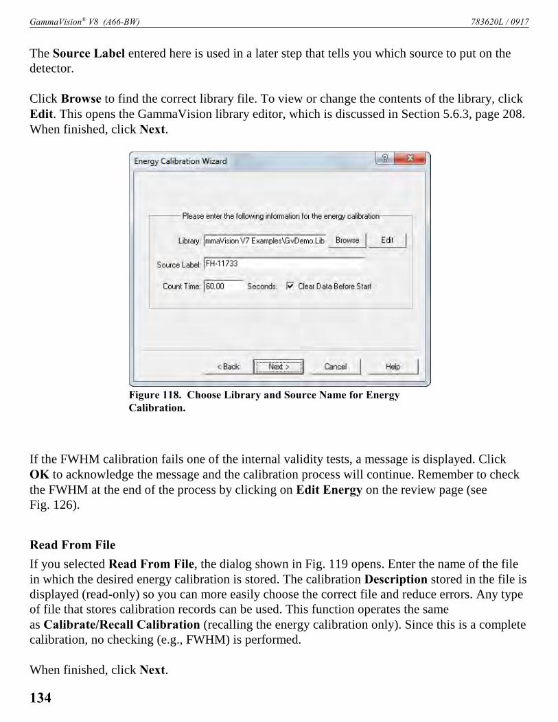
GammaVision® V8 (A66-BW) 783620L / 0917
Figure 118. Choose Library and Source Name for EnergyCalibration.
The Source Label entered here is used in a later step that tells you which source to put on thedetector.
Click Browse to find the correct library file. To view or change the contents of the library, clickEdit. This opens the GammaVision library editor, which is discussed in Section 5.6.3, page 208.When finished, click Next.
If the FWHM calibration fails one of the internal validity tests, a message is displayed. ClickOK to acknowledge the message and the calibration process will continue. Remember to checkthe FWHM at the end of the process by clicking on Edit Energy on the review page (seeFig. 126).
Read From File
If you selected Read From File, the dialog shown in Fig. 119 opens. Enter the name of the filein which the desired energy calibration is stored. The calibration Description stored in the file isdisplayed (read-only) so you can more easily choose the correct file and reduce errors. Any typeof file that stores calibration records can be used. This function operates the sameas Calibrate/Recall Calibration (recalling the energy calibration only). Since this is a completecalibration, no checking (e.g., FWHM) is performed.
When finished, click Next.
134

783620L / 0917 5. MENU COMMANDS
Figure 119. Select the File that Contains the Desired EnergyCalibration.
5.3.8.2. Efficiency and Efficiency-plus-TCC Calibrations — Setting Up a New Calibrationor Recalling from File
Create New
If you chose to create a new efficiency or efficiency-plus-TCC calibration, the dialog shown inFig. 120 opens. Use this dialog to enter the source Certificate File, Library file, Source Label,and TCC Calibration Method settings.
When performing this calibration on the MCB, you must enter the live-time preset (CountTime) in seconds. In addition, you might also wish to mark the Clear Data Before Start check-box. The counting time must be long enough to accumulate well-formed peaks with low count-ing uncertainty. This is especially important for TCC calibration, which uses the summed peaksin the calculations.
Also note that your library and TCC table should include only peaks that exist in the spectrum.
To use the spectrum currently in the MCB, unmark the Clear Data Before Start box. This isuseful if the same source is used for both energy and efficiency calibration.
135

GammaVision® V8 (A66-BW) 783620L / 0917
Figure 120. Create a New Efficiency Calibration.
The Source Label entered here is used in a later step that tells you which source to put on thedetector.
Certificate File
Use the Browse button to find the correct certificate. To make changes to the certificate, clickEdit. This opens the wizard’s Certificate File Editor dialog, shown in Fig. 121.
The certificate file is the same as the efficiency standard file, except that the contents of theefficiency field are not used here and all fields must have valid contents. The certificate filealso has the EFT extension. Tables with all fields entered can be used for both the calibrationwizard and the efficiency calibration (Calibrate/ Efficiency...). Any energy in the .EFT file thatis not completely filled in will be ignored by the wizard. The file contains all the data needed toperform an efficiency or efficiency-plus-TCC calibration using this standard source. This file canbe created here, with the Efficiency calibration sidebar (see Section 5.3.3.12) or with an ASCIItext editor.
The table contains the following columns:
1) Isotope name (same as library).2) Gamma-ray energy (keV).3) Activity in Bq or ìCi at the date and time specified in column 6.4) Gammas/sec for this energy at the specified date and time.
136

783620L / 0917 5. MENU COMMANDS
Figure 121. Edit Wizard Certificate File.
5) 1-Sigma Uncertainty for this nuclide.6) Calibration date and time for the gammas/sec calibration. The gammas/sec are automatically
decay corrected from the date/time in column 4 to the date/time of the spectrum acquisition.7) Half-life of this nuclide in days.8) Branching ratio (yield) as gammas/100 disintegrations.
To add an energy to the table, enter the values directly or click Select from Lib, then click AddNew.
To delete an energy, select the energy and click Delete.
To change the values for an energy, select the energy, enter the new values directly or clickSelect from Lib, then click Update to record the changes (you must click Update or thechanges will not be made).
When finished, click Save As... to rewrite the new file to disk. To discard the changes you havejust made, click Cancel; a dialog will verify that you want to discard.
137

GammaVision® V8 (A66-BW) 783620L / 0917
Library
Click Browse to find the correct library file. For TCC calibrations, the library (.LIB or .MDB) fileand TCC table should include only the nuclides present in the spectrum.
To view or change the contents of the library, click Edit. This opens the GammaVision libraryeditor, which is discussed in Section 5.6.3, page 208.
When finished, click Next.
TCC Calibration Method
The Single Point Source Method uses a point source with all the nuclides needed in one source.The point source is normally a small area (1 mm–2 mm diameter). Larger sources can be used ifthey are more than a few centimeters from the detector. An example of the nuclide mixture isgiven below.
The Single Extended Source Method uses bulk or large-volume sources such as Marinellibeakers or bottles with all the nuclides needed in one source.
The source must be a mixture of nuclides with gamma rays that do not have true coincidencesumming and nuclides with gamma rays that do have summing. The energies of the gamma raysmust extend over the range of interest for the unknown samples. A mixture of 109Cd, 113Sn, 139Ce,203Hg, 134Cs, 137Cs, 88Y, and 54Mn will be sufficient for most situations. 241Am can be added forlower energies.
NOTE 60Co should not be added because of the interference with gamma rays from 134Cs.
The absorber present/not present selection determines the low-energy fitting function. Theefficiency for low-energy gamma rays depends on the absorbing material between the detectorand the source. The absorbing material and thickness are not important. GammaVision willautomatically account for the loss in the fitting process if the absorber is present. The low-energycoefficients are listed as the last 2 (of 6) of the TCC polynomial coefficients and are zero forabsorber Not Present.
The selection of point or extended source and absorber present or not may depend on the specificdetector type and container material. Use the Next and Back buttons on the Calibration Wizardto view the calibration results and return to this page to change the settings until the bestcalibration fit is achieved.
When finished, click Next.
138

783620L / 0917 5. MENU COMMANDS
Figure 122. Select the File Containing the Desired EfficiencyCalibration.
Read From File — Efficiency
If you selected Read From File for the efficiency calibration, the dialog shown in Fig. 122opens. Enter the name of the file in which the desired efficiency calibration is stored. The cali-bration Description stored in the file is displayed (read-only) so you can more easily choose thecorrect file and reduce errors. Any type of file that stores calibration records can be used.
This function operates the same as Calibrate/Recall Calibration (recalling the efficiencycalibration only).
When finished, click Next.
Read from File — TCC
If you selected Read From File for the TCC calibration, the dialog shown in Fig. 123 opens.Enter the name of the file in which the desired TCC calibration is stored. Since the TCC islinked to the efficiency, this will load both the efficiency and the TCC calibration parameters. Besure to use the same file for the efficiency calibration (Read From File — Efficiency) and TCCcalibration; otherwise, the TCC calibration loaded may not be complete and will not produceaccurate results.
The calibration Description stored in the file is displayed (read-only) so you can more easilychoose the correct file and reduce errors. Any file that stores calibration records can be used.
139

GammaVision® V8 (A66-BW) 783620L / 0917
Figure 123. Select the File that Contains the Desired TCCCalibration.
Figure 124. Position the Source for Energy Calibration.
When finished, click Next.
5.3.8.3. Performing the New Energy Calibration
If you chose to create a new energy calibration, the dialog shown in Fig. 124 opens. Position thesource and click OK to begin spectrum acquisition. If the buffer is selected, the current spectrumin the buffer is used.
When spectrum collection is complete (or the buffer is used), the energy and FWHM calibrationis performed. If successful, the wizard goes on to the next step.
140

783620L / 0917 5. MENU COMMANDS
Figure 125. Position the Source for the Efficiency orEfficiency-plus-TCC Calibration.
If the energy calibration process detects a severe error, an error message is displayed. Click OKto acknowledge the error. The calibration process will stop at this point.
If the energy calibration process detects a minor error, a warning message is shown. Click OK toacknowledge the warning and remember that this warning was given. The calibration processwill continue as normal. When the final review screen is displayed (Fig. 126), click Edit Energyto review the cause of the error and correct it if needed (see Section 5.3.8.5).
5.3.8.4. Performing the New Efficiency or Efficiency-plus-TCC Calibration
If you chose to create a newefficiency or efficiency-plus-TCC calibration, the wizardasks for the next source to bepositioned (see Fig. 125). ClickOK to begin spectrum acqui-sition. If the buffer is selected,the current spectrum in thebuffer is used.
If the efficiency calibrationprocess detects a severe error, an error message is displayed. Click OK to acknowledge theerror. The calibration process will stop at this point.
5.3.8.5. Reviewing the Calibration Wizard Results
The final screen in the calibration wizard is the review screen shown in Fig. 126. This shows theplots of the results of all the calibration steps. The TCC functions are not plotted, but indicatedas Tcc Calibrated or Uncalibrated.
When the TCC calibration is performed, it includes recalculating the efficiency function, there-fore, the efficiency curve (upper right) might not appear to be a good fit to the experimentalpoints. This is because the total efficiency function is the combination of all the differentfunctions.
To review or change the energy or FWHM calibration, click Edit Energy. This opens the com-plete energy calibration dialog as explained in Section 5.3.2, page 105. If any changes are made,the efficiency (and TCC) calibration should be repeated. If you did not select TCC, the effi-ciency calibration can be redone by clicking on Edit Efficiency. This will open up the completeefficiency calibration dialog as explained in Section 5.3.3, page 114. This does not redo the TCCcalibration.
141

GammaVision® V8 (A66-BW) 783620L / 0917
Figure 126. Review the Calibration Results.
Alternatively, you can change a calibration by clicking on Back to return to previous wizardscreens. Click Back to return to the efficiency dialog, then Back again to return to the energydialog.
NOTE If the spectrum currently in the MCB is the right spectrum, be sure to unmark the ClearData Before Start checkbox.
Once you have reset the starting parameters as needed, the process will continue on as beforewith the spectrum collection or file recall.
The calibration is now stored with the MCB or buffer, but not on disk. Use the Save Calibrationbutton to save the calibration to a file. This should always be done to preserve the calibration forlater use.
To complete the calibration wizard and close the dialog, click Finish. (Cancel operates the sameas Finish.)
To validate the TCC Calibration, analyze the calibration spectrum with the new Efficiency/TCCcalibration and the TCC option enabled in the analysis settings. The calculated nuclide activityshould be very close to the source certificate values. The TCC calibration correction can beassessed by comparing the Peak Branching Ratios from the library to the corrected BranchingRatios displayed in the Library usage section of the GammaVision report.
142

783620L / 0917 5. MENU COMMANDS
Figure 127. Calculate Menu.
Figure 128.
Figure 129. Select a Time Slice of List Mode Data.
5.4. Calculate
The Calculate menu (Fig. 127) provides useful analytical tools forspectrum manipulation. Smooth and Strip... are only available inbuffer windows.
5.4.1. Settings...
This dialog (Fig. 128) allows you to set the “x” factor in the PeakInfo calculation of full width at 1/x maximum (FW[1/x]M) for theROI marked by the cursor (see Section 5.4.3). In addition, you canset the number of background channels used on each side of thepeak. The background is subtracted before starting the calculation.Enter the factor x, an integer from 2 to 99. This numberwill be retained and used until changed. (Peak Infoalways displays the FWHM, so an x of 2 is not useful.)The number of Background Points ranges from 1 to 5,and the default value is 3.
5.4.2. List Data Range...
Use this dialog (Fig. 129) to retrieve aspecified time slice of data from a ListMode (.LIS) file that has been recalledinto a buffer window. GammaVisionsamples the list mode data stream every250 milliseconds of real time, and candisplay the data with a granularity of1 second (see the List Mode discus-sion in Section 1.6).
Click to highlight the desired start andend Date/Time values, then adjust themby clicking the up/down buttons; or setthe desired Data Start Date/Time and enter the time slice Duration in whole seconds.24 Toretrieve the data, click Apply. Click Increment to add the next more data to the currently dis-played time slice; set the Duration, then click Increment. To save a time slice in any Gamma-Vision file format (i.e., as list files and/or spectrum files), use the Save commands.
24The analogous JOB stream command, SET_RANGE (page 410), can use fractional real times and durations.
143

GammaVision® V8 (A66-BW) 783620L / 0917
Figure 130. Peak Info Beneath Marker andAbove Peak.
To redisplay the complete data set rounded down to the nearest whole second, click Restore. Toredisplay the entire data set without rounding, close and recall the .LIS file.
This command is duplicated by the List Data Range button on the toolbar.
5.4.3. Peak Info
This command operates when the marker ispositioned in a peak or in an area marked asan ROI. It displays the following informationin a pop-up box and on the SupplementaryInformation Line (Fig. 130):
! If the spectrum is not calibrated, thecentroid channel, FWHM, FW1/xM(all in channels), gross area, net area,and net-area uncertainty are displayedfor the ROI.
! If the spectrum is calibrated, thecentroid channel, FWHM, FW1/xMin channels and calibration units (e.g.,energy), library “best match” energyand activity, gross area, net area, andnet-area uncertainty are displayed forthe ROI.
If the Detector is acquiring data, the values displayed are continuously updated.
NOTE If the marker is in an ROI, peak information is displayed whether or not the area is adetectable peak. If no ROI is marked, the peak limits are the same as the limits for theROI Insert button on the Status Sidebar. If a peak is detected, its information isdisplayed (otherwise a “could not fit peak properly” message is displayed).
To close the pop-up box, click it or press <Esc>.
This command is duplicated by the Peak Info command on the right-mouse-button menu and bydouble-clicking the mouse in the ROI.
144

783620L / 0917 5. MENU COMMANDS
Figure 131. Calculation Details.
(15)
(16)
5.4.3.1. Calculation
The program subtracts the calculated background, channel by channel, and attempts a least-squares fit of a Gaussian function to the remaining data. If unsuccessful, it displays “Could NotProperly Fit Peak.” If successful, the centroid is based on the fitted function. The reportedwidths are linearly interpolated between the background-subtracted channels. The spectrumcomponents used in the background calculation are illustrated in see Fig. 131.
The background on the low channel sideof the peak is the average of the first nchannels of the ROI, where n is the numberof background points selected on the dialogunder Calculate/Settings... (Section 5.4.1).The channel number for this backgroundpoint is the midpoint fractional channel ofthe n points. The background on the highchannel side of the peak is the average ofthe last n channels of the ROI. The channelnumber for this background point is also themidpoint fractional channel of the n points.These (n!1) points on each side of the peakform the end points of the straight-linebackground.
The background is given by the following:
where:B = the background areal = the ROI low limith = the ROI high limitCi = the contents of channel in = the number of background points
The gross area is the sum of all the channels marked by the ROI according to the following:
145

GammaVision® V8 (A66-BW) 783620L / 0917
(17)
(18)
(19)
where:Ag = the gross counts in the ROIl = the ROI low limith = the ROI high limitCi = the contents of channel i
The adjusted gross area is the sum of all the channels marked by the ROI but not used in thebackground according to the following:
where:Aag = the adjusted gross counts in the ROIl = the ROI low limith = the ROI high limitCi = the contents of channel in = the number of background points
The net area is the adjusted gross area minus the adjusted calculated background, as follows:
The uncertainty in the net area is the square root of the sum of the squares of the uncertainty inthe adjusted gross area and the weighted error of the adjusted background. The backgrounduncertainty is weighted by the ratio of the adjusted peak width to the number of channels used tocalculate the adjusted background. Therefore, net peak-area uncertainty is given by:
where:Aag = the adjusted gross areaAn = the net areaB = the background areal = the ROI low limith = the ROI high limitn = the number of background points
146

783620L / 0917 5. MENU COMMANDS
(20)
Figure 132. Input Count RateMeter.
The counting activity, cA, is calculated as:
where:Percent = Gammas per 100 disintegrations (from library list)Net Counts = Net counts in the peakLive Time = Live time in seconds
5.4.4. Input Count Rate
This command is supported by most newer ORTEC MCBsand disabled for unsupported units. It displays or hides theinput count rate meter (Fig. 132) in the upper left corner ofthe spectrum window.25 (This is input count rate used for thedead-time calculation, not the number of processed pulses.)This command is also on the right-mouse-button menu.
Detector windows show the current (live) input count rate, whether or not the MCB is currentlyacquiring data. Buffer windows show the input count rate when the spectrum was (1) transferredto the buffer from the MCB or (2) saved to disk.
5.4.5. Sum
The Sum function performs its calculation as follows, and displays the sum on the MarkerInformation Line:
1) If the marker is not in an ROI, the counts in all data channels in the buffer (e.g., channel 1to the maximum channel currently selected) are summed.
2) If the marker is in an ROI, the sum of the data channels in the ROI is shown on the display.This is the same as the gross counts in the Peak Info display, but can be used on wider ROIs.
3) You can also sum a region by marking it with a rubber rectangle, then selecting Sum. This isillustrated in Fig. 133.
25Note that if the full spectrum view is positioned in the same corner, it can obscure the Input Count Rate box.
147

GammaVision® V8 (A66-BW) 783620L / 0917
(21)
5.4.6. Smooth
The Smooth command is available in buffer windows only. It transforms the data in the bufferspectrum according to a five-point, area-preserving, binomial smoothing algorithm. That is, theexisting data is replaced, channel-by-channel, with the averaged or smoothed data as follows:
where:Si = the smoothed data in channel iOi = the original data in channel i
5.4.7. Strip...
This command (Fig. 134) strips the specified disk spectrum from the spectrum in the buffer andstores the result in the buffer. Select a File name and Stripping Factor, and click on OK.
NOTE Any valid spectral data file can be selected, but it must contain the same number ofchannels as the buffer.
Figure 133. Summing the Channels Within aRubber Rectangle.
148

783620L / 0917 5. MENU COMMANDS
Figure 135. Analyze Menu.
The strip factor is a real number that is multiplied, channel by channel, by the disk spectrumbefore being subtracted from the buffer. If the Use Ratio of Live Times box is marked, the stripfactor is calculated as the ratio of the live time of the buffer spectrum divided by the live time ofthe disk spectrum. Unmarking the Use Ratio box allows you to enter a factor, which can benegative, in which case the spectra are added.
NOTE The live time and real time are not changed by any strip operation. Also, the peakuncertainty (see Section 6.3.4) does not include the stripped areas and might notrepresent the true uncertainty.
5.5. Analyze
The Analyze menu (Fig. 135) contains commands that allowyou to analyze all or part of a spectrum on the screen or ondisk. The results can be displayed in both graphic and textforms. In the interactive analysis mode, peaks can be added,deleted, or shifted in energy. You can perform these com-mands on data in a buffer window or in a Detector if theDetector is not acquiring data. If a command is not available,it is disabled (gray). Interactive in viewed area... is activeonly when the Expanded Spectrum View displays #4096channels (zoom in on a portion of the spectrum to activatethis command).
Figure 134. Choose Strip Spectrum.
149

GammaVision® V8 (A66-BW) 783620L / 0917
Figure 136. SettingsSubmenu.
5.5.1. Settings
This opens the submenu shown in Fig. 136. The user-controlled factors in the analysis are defined in thesedialogs, and the analysis results can be captured in theanalysis report discussed in Chapter 7.
NOTE Version 7 and 8 analysis settings (.SDF) files arenot compatible with earlier versions ofGammaVision.
5.5.1.1. Sample Type...
This opens the multi-tab Sample Type Settings dialogdiscussed in the following sections. The fields on thisset of screens define a complete set of GammaVision analysis settings. Once defined, they can besaved to a Sample Description (.SDF) file. This .SDF file can then be used in .JOB files, in theQA analysis, as the acquisition preset default in Ask on Start, as the current defaults, and inother places within GammaVision.
To create an .SDF file, complete all screens of the dialog, then return to the Sample tab. Clickthe Save As... button in the upper right of the dialog; this will open a standard file-save dialog.Enter the path (if necessary) and new filename, then click OK to return to the Sample tab. Clickagain on OK to close the Sample Type Settings dialog.
NOTE Although this dialog has multiple tabs, any changes to the current set of “working”parameters for the selected Detector will not take effect until you click OK. To retainthe current working parameters, click on Cancel.
Sample Tab
Sample settings (Fig. 137) are those whose values are generally different for each sample type.When an .SDF file is recalled, the date of Creation and last date the file was updated (Edition)are displayed. Whenever the file is changed, the edition date is updated.
The Description is used to identify the sample-type file, and can be 64 characters long.
Clicking on the Presets button opens a Presets dialog corresponding to the available presets forthis MCB, as discussed in Acquire/MCB Properties....(Remember that these default presets canbe used automatically if the appropriate Ask on Start box in checked under Acquire/ Acquisi-tion Settings...; see Section 5.2.1 for more information.)
150
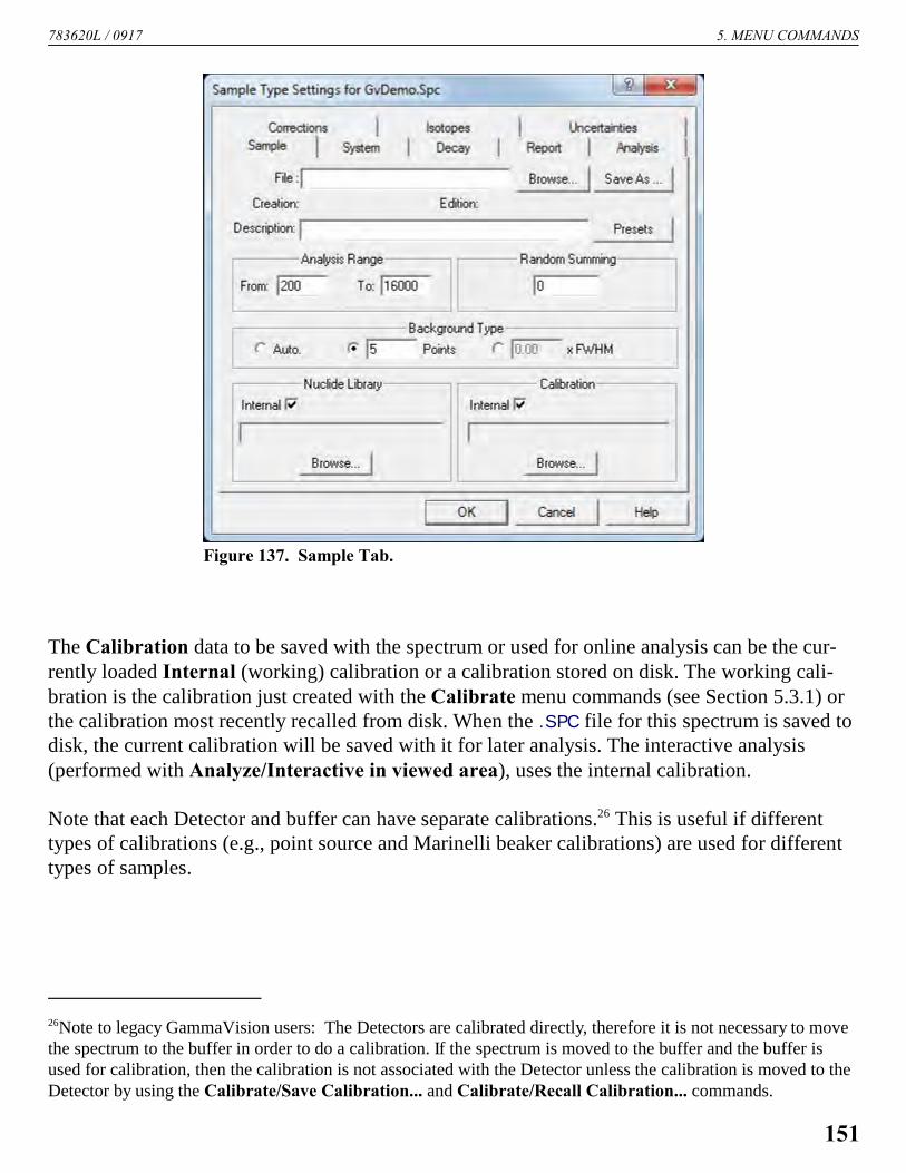
783620L / 0917 5. MENU COMMANDS
Figure 137. Sample Tab.
The Calibration data to be saved with the spectrum or used for online analysis can be the cur-rently loaded Internal (working) calibration or a calibration stored on disk. The working cali-bration is the calibration just created with the Calibrate menu commands (see Section 5.3.1) orthe calibration most recently recalled from disk. When the .SPC file for this spectrum is saved todisk, the current calibration will be saved with it for later analysis. The interactive analysis(performed with Analyze/Interactive in viewed area), uses the internal calibration.
Note that each Detector and buffer can have separate calibrations.26 This is useful if differenttypes of calibrations (e.g., point source and Marinelli beaker calibrations) are used for differenttypes of samples.
26Note to legacy GammaVision users: The Detectors are calibrated directly, therefore it is not necessary to movethe spectrum to the buffer in order to do a calibration. If the spectrum is moved to the buffer and the buffer isused for calibration, then the calibration is not associated with the Detector unless the calibration is moved to theDetector by using the Calibrate/Save Calibration... and Calibrate/Recall Calibration... commands.
151

GammaVision® V8 (A66-BW) 783620L / 0917
The filename of the Nuclide Library to be used in the spectrum analysis can be the Internal(working) library or a library on disk. The working library is the library from Library/SelectFile..., and will include any modifications made during the interactive analysis mode.
The Background Type can be set to Auto, X-Points, or X * FWHM. These are explained inmore detail in Section 6.3.1.
Random Summing is the random summing correction factor discussed in Section 6.11. Enteringzero turns this correction off.
The Analysis Range, in channels, can be entered. This is usually used to eliminate analysis ofthe ends of the spectrum that do not contain useful data. The Analysis Range should be as wideas possible because the automatic energy recalibration feature (see Section 6.3.6) requiresseparated library peaks to work properly. Also, the correlation of lines from a single nuclidedone by the analysis is defeated if the energy range analyzed does not include all the lines.
System Tab
System settings are those settings that are generally the same from sample to sample. However,all of these entries except the Laboratory and Operator names can be different for each sampletype. The dialog is shown in Fig. 138.
The Laboratory name, composed of any 64 characters, is printed as the second line on eachpage of the report. The spectrum name is printed on the next line.
The Operator name is the name of the person operating the system. This name will appear onthe analysis reports. This field defaults to the user name entered during Windows installation.
MDA Type — This allows the selection of the type of MDA calculation to be used as themethod of calculating the MDA to be on the report. The MDA is a measure of how small anactivity could be present and not be detected by the analysis. Many factors affect the MDA,which is reported in units of activity, such as becquerels. The calibration geometry, backgrounds(system and source-induced), detector resolution, and particular nuclide all seriously affect theMDA reported. Section 6.9 provides explanations of the different MDA formulas used byGammaVision.
In the Library section, Match Width sets the maximum amount by which a peak centroid candeviate from the nearest library peak energy and still be associated with that library peak. Thevalue entered is multiplied by the FWHM at the peak energy to get the width used.
152

783620L / 0917 5. MENU COMMANDS
Figure 138. System Tab.
NOTES If the value is too small, some spectrum peaks will be misidentified due to statisticalvariation in the centroid; if it is too large, some library peaks will be incorrectlyidentified.
During efficiency calibration, the net peak area calculation can be affected by thelibrary Match Width setting in effect at the time the calibration is performed. Beforestarting an efficiency calibration, make sure the Match Width is set to the samevalue you will be using during analysis. Most users will keep the default setting, 0.5.If using a different setting, we recommend a value between 0.4 and 0.75.
If the Match Width is set to a value other than 0.5, the value will be printed on the report.
The Fraction Limit is one of the parameters used to determine the presence or absence of anuclide. The sum of the emission probabilities of the peaks in the spectrum identified with thenuclide is divided by the sum of the emission probabilities of all peaks of the nuclide in theenergy range being analyzed. If the result is greater than the fraction limit, the nuclide is markedas being present. To turn off this test, set the limit to zero.
153

GammaVision® V8 (A66-BW) 783620L / 0917
File for Suspected Nuclides — In the list of unknown peaks, there is a column for suspectednuclides. This is the closest energy in the library file to the unknown peak’s energy. Suspectednuclides are identified in GammaVision using a suspected-nuclide library. This file is a libraryfile (see Section 5.6). Typically, it is a much larger file than the analysis library file. The identi-fication window is also much larger for this list than for the analysis library. This list might con-tain common lines (such as 511 keV or 40K) that are present in the spectrum, but not desired inthe analysis.
If the suspected-nuclide library contains the same lines as the analysis library, a nuclide whoseenergy is shifted just out of range for the analysis (the default is 0.5 × FWHM) will be marked assuspected on the unknown list.
The File for Suspected Nuclides must not have the same name as the analysis library file. Ifnecessary, make a copy of the analysis library file with a new name.
The Units section allows the selection of either becquerels (Bq) or microcuries (ìCi) as the baseunits, a Multiplier and Divisor to scale the numbers up or down.
The units label is printed at the top of the activity columns on the report and should reflect thevalues chosen; that is, if ìCi is chosen with a multiplier of 1000, then “nanocuries” should beentered in the Activity field. If the sample quantity is entered later (see Acquire/AcquisitionSettings... or File/Settings...), the units for quantity (weight or volume) are entered in the Sizefield. The combined label (activity/quantity) is limited to 14 characters. Optionally enter a1-sigma sample Size uncertainty (+/-) between 0% and 1000%.
The Multiplier, Divisor, and sample Size values are used to generate the Activity scaling factorlisted in the Analysis Parameters section of the report, and used by the NPP32 and ENV32analysis engines to calculate the report’s Summary of Library Peak Usage table.
The PEAK SEARCH SENSITIVITY sets the sensitivity for the peak search used in the PeakSearch (Section 5.5.2), Interactive in viewed area (Section 5.5.7), and the full-spectrumanalysis (Section 5.5.4). Before a suspected peak is accepted, the magnitude of the seconddifference must be greater than the weighted error of the channel counts. The PEAK SEARCHSENSITIVITY is a multiplicative factor used in error weighting.
The sensitivity can be set at any integer value from 1 to 5, with 1 the most sensitive (that is, “1"finds the most peaks). A value of 1 will find small peaks, but will also “find” many false peaks.A value of 5 will locate all the large peaks, but might miss some of the smaller peaks. If toolarge, some small peaks will be missed. In the interactive mode, many regions will be deconvo-luted unnecessarily if the value is too sensitive. The parabolic background method is disabled forenergies above 200 keV if the sensitivity is set to 1.
154

783620L / 0917 5. MENU COMMANDS
Figure 139. Decay Tab.
Decay Tab
The Decay tab is shown in Fig. 139. This dialog shows all the decay options and date/time entryfields.
Mark the checkboxes in the Decay Correction section to enable or disable decay correctionDuring Acquisition and decay correction to a given date and time. Both of these affect thereport of the analysis of the total spectrum.
The Collection date and time can also be entered under Acquire/Acquisition Settings....
Mark the checkbox in the Sample Collection section and enter the times for sample collection.These dates/times are the start time of the sample collection and the stop time of the samplecollection. For example, for air filters, the start time is the time when the air flow is started andthe stop time is when the air flow is stopped. These times are used to calculate the buildup of theactivity in the sample. It is assumed that the spectrum is not collected during the build-up time.
The correction for the build-up is given in Section 6.10.5.
155

GammaVision® V8 (A66-BW) 783620L / 0917
Figure 140. Report Tab.
Report Tab
This screen (Fig. 140) controls the contents, destination, and some details of the output reportdiscussed in Chapter 7.
Reporting Options
Select one or more Reporting Options by marking the checkboxes. If there is not enough infor-mation for GammaVision to generate one or more of the requested options, the software canprint another option if there is enough information for it. For example, suppose a nuclide activityreport is the only report option selected. If the spectrum has not been efficiency calibrated, theactivities cannot be calculated. In this case, GammaVision will instead print the peak list becausethere is sufficient information to do that.
Output examples for all the reporting options are discussed in Chapter 7.
156

783620L / 0917 5. MENU COMMANDS
The ISO NORM ReportNote that analysis flags in the library editor and in the analysis parameters file, b30winds.ini
(n30winds.ini for NAI32), are treated differently between GammaVision’s standard analysisand its ISO NORM implementation. The ISO NORM report contents are discussed andillustrated in Section 7.7.12.
LibraryNo-MDA flag
Note that the “No MDA” flag functions differently for ISO NORM than for thestandard GammaVision analysis. If an isotope flagged as “No MDA” is not detectedin the sample, it is not reported in the standard GammaVision report sections unlessthe Directed Fit flag is turned on. However, the isotope is always reported in the ISONORM table.
b30winds.ini ( n30winds.ini for NAI32)The b30winds.ini and n30winds.ini files include settings for the ISO NORM report(Section A.2.2), e.g., settings for the three probability factors, á, â, and ä, plus a flag toreport MDA if the activity is less than the CL (In ISO NORM Table, print MDA if y < y*).The probabilities for these factors are set by default to 0.05 for 5% error, with a range of1.0E!6 to 1. If the input values are outside this range, 0.05 is used. Changing the defaultparameters requires editing the probability alpha, probability beta, and probability
gamma flags in the b30winds.ini or n30winds.ini files (see Section A.2.2). By default, ifthe CL is greater than the activity, the MDA is reported. However, the In ISO NORM
Table, print MDA if y < y* flag can be set to false so that the activity and associateduncertainty are always reported.
Following are additional b30winds.ini/n30winds.ini flags that operate differently for theISO NORM calculations than for other parts of the GammaVision report:
Print MDA in Nuclide SummaryWhen the ISO NORM reporting option is selected, this flag (page 443) is ignored sothe format of the ISO NORM table remains fixed.
Nuclide Summary MDA TextThis flag (page 444) is ignored; the “MDA” title cannot be changed to read “CL” inthe ISO NORM section of the report.
Background Width for MDAThis flag (page 443) is not used in ISO NORM calculations.
157

GammaVision® V8 (A66-BW) 783620L / 0917
Second MDA TypeThis flag (page 443) is ignored because there is no second MDA in the ISO NORMtable. A second MDA can still be calculated through the regular GammaVisionanalysis.
Allow MDA Type ChangeThis flag (page 439) is ignored in the ISO NORM table because there is no otherMDA type.
Uncertainty Reporting
The Confidence level multiplier shown here is used on the report only. All internal checks onpeak uncertainty are done at the 1-sigma level. See Section 6 for details on the total uncertaintycalculation. The uncertainty can be in Activity (e.g., 200 Bq ± 10 Bq) or Percent (e.g.,200 Bq ± 5%). If Counting is selected, counting uncertainty will be printed. If Total is selected,both the counting and total uncertainty will be printed.
Output
When GammaVision performs an analysis, a spectrum files is automatically created with theextension of .AN1. In addition, the results are written to a .UFO file and an ASCII-format .RPT
file that use the same base filename as the spectrum file. Use the Output section of the Reporttab to send the appropriate results file to any Windows-supported Printer available to the com-puter, a disk File, a Program, or the optional GammaVision Report Writer. You can alsochoose to display the analysis results graphically onscreen, in the same form as for Analyze/Display analysis results (Section 5.5.6).
When File is selected, you can specify a new or existing filename; click Browse... and select anexisting file to overwrite with the new output data; or leave the default asterisk (*) in the file-name field. In this case, the report filename will remain the spectrum filename with the extension.RPT.
When Program is selected, you can choose any Windows program to be run with the reportfilename as an argument on the command line. The report filename sent to the program is thespectrum filename with the extension .RPT. The default program is Windows Notepad,Notepad.exe. In this case, when the analysis finishes, Notepad automatically starts, and opensthe .RPT file. (You can also use Notepad to save the .RPT file to a different filename if desired orprint the report.) The analysis is not complete until you close the selected program.
Instead of Notepad.exe, any user-written program (actually, any program that can read ORTEC.RPT files) can be selected here. In this case, the .RPT filename is used as an argument on thecommand line of the specified program.
158

783620L / 0917 5. MENU COMMANDS
Figure 141. Analysis Tab.
The name of the .UFO file corresponds to the spectrum file from which it derives. A user-writtenprogram can read the report filename from the command line, change the extension to .UFO, andread the analysis results from the .UFO file.
The Report Writer check box is only active if the GammaVision Report Writer (A44-BW) isinstalled. This option uses an Access database and SAP® BusinessObjects Crystal Reports™ toproduce the desired report. Click Browse... to select the report template to be used (see theGammaVision Report Writer’s user manual for a complete discussion of templates).
Analysis Tab
Use this screen (Fig. 141) to select the Analysis Method, Additional Error, Analysis, andPeak Stripping options to be used. The actual analysis is done by a separate program referred toas an analysis engine.
159

GammaVision® V8 (A66-BW) 783620L / 0917
Analysis Method
The analysis engine for the normal analysis is named WAN32; GammaVision also offers theROI32, GAM32, NPP32, and ENV32 engines.
See Chapter 6 for more information on the analysis programs.
GammaVision also accommodates user-supplied analysis programs. The program must be ableto read the spectrum name from the command line. There are no other restrictions, but if theprogram does not produce a results file in the .UFO format, the display results functions and theGammaVision Report Writer database will not work. All the analysis options can be taken fromthe .SPC file. The analysis program should also produce an ASCII report file so the report can beprinted by the Windows print spooler.
Additional Error
The parameters in the Additional Error section are used in the calculation of the total uncer-tainty. Total uncertainty is composed of error estimates that follow a normal distribution anderror estimates that follow a uniform distribution over a range. Most errors in gamma spectro-scopy, whether systematic or random, follow a normal distribution. Error estimates are includedfor counting, random summing, absorption, nuclide uncertainty, efficiency, and geometry. Enteradditional errors (%) related to the measurement that follow a normal distribution at the 1-sigmalevel. Enter uniform distribution errors (%) at the complete range of the uniform error limit. Thatis, if the likelihood of an uncertainty is uniform over 3% of the reported results, enter 3.0 in thisfield. The error estimates from all corrections are explained in Section 6.12.
Peak Stripping
When Peak Stripping is enabled, the analysis will perform the library-based peak deconvolutionor “peak interference correction” described in Section 6.5.5. Briefly, this will separate peak areasthat are too close together to be accurately separated by mathematical deconvolution. Gamma-Vision supports two types of peak stripping: Library Based and Manual Based. In LibraryBased peak stripping, the program automatically detects overlapped peaks and the associatedpeaks needed. The program then performs the peak stripping using these peaks. In ManualBased peak stripping, you determine the overlapping peaks and the associated peaks. Theassociated peaks are given in the Second Library and the analysis peaks are given in the ThirdLibrary.
The availability of peak-stripping options depends on the analysis engine you choose. SeeSection 6.2 for a discussion of the analysis engines, a decision matrix, and selection guidelines.
WAN32 offers both the Library Based and Manual Based options, however, you can onlychoose one option at a time (or leave the boxes unmarked to perform no stripping).
160

783620L / 0917 5. MENU COMMANDS
When GAM32 or ROI32 is selected, the Library Based Peak Stripping and Directed Fitmethods are turned off and the selections disabled.
When NPP32, ENV32, or NAI32 is selected, the Library Based Peak Stripping option isturned on and cannot be disabled. If analysis without library-based peak stripping is desired,then either WAN32, GAM32, or ROI32 analysis engines must be used.
Analysis
Only peaks with 1-sigma counting uncertainty less than the Peak Cutoff are used to calculatenuclide activity or report as unidentified. Library peaks with uncertainty higher than the PeakCutoff may still be reported in different sections of the analysis report for different analysisengines based on parameter settings in the b30winds.ini (n30winds.ini for NAI32) file; seeSection A.2.2.
Click True Coincidence Correction to enable TCC.
! If the Detector has not been calibrated for TCC, the correction is automatically turned offin the analysis.
! If preparing to analyze a saved spectrum, be sure it contains a TCC calibration; other-wise the analysis results may be incorrect. To check a spectrum file for TCC calibration,recall it, step through the Calibration Wizard , and on the final screen (Fig. 126,page 142) confirm that the lower-right window says TCC Calibrated.
Click Directed Fit to allow for negative peak areas in low-level spectra. The following rulesshould normally be followed when using directed fit:
! Preferentially use the ENV32 analysis engine (NAI32 for sodium iodide) unless a featureof one of the other engines is required. ENV32 is required when analyzing complicatedspectra with overlapping peaks or large libraries.
! Use NPP32 or WAN32 only for relatively simple spectra that contain only singlet peaks.
! The Peak Cutoff is typically set to accept good quality peaks. However, a high value(i.e., 1000) may be used in some cases to preferentially retain peaks found using thenormal peak search method rather than resorting to Directed Fit so that peak stripping isapplied using the library configuration.
For more information, see the Directed Fit discussion in Section 6.3.2.2.
161
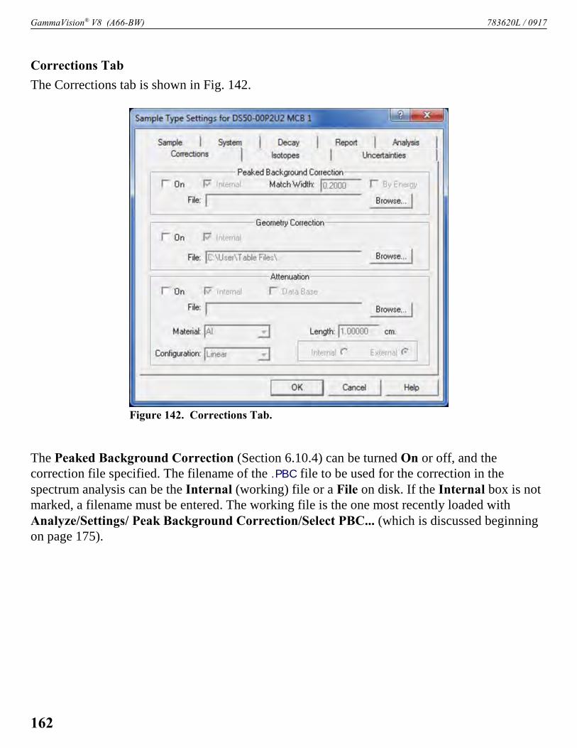
GammaVision® V8 (A66-BW) 783620L / 0917
Figure 142. Corrections Tab.
Corrections Tab
The Corrections tab is shown in Fig. 142.
The Peaked Background Correction (Section 6.10.4) can be turned On or off, and thecorrection file specified. The filename of the .PBC file to be used for the correction in thespectrum analysis can be the Internal (working) file or a File on disk. If the Internal box is notmarked, a filename must be entered. The working file is the one most recently loaded withAnalyze/Settings/ Peak Background Correction/Select PBC... (which is discussed beginningon page 175).
162
783620L / 0917 5. MENU COMMANDS
Adjust the Match Width as desired. For the By Energy option, when not using a library youmay wish to use a greater PBC match width. It may be useful to perform test acquisitions basedon your application.
! If the By Energy checkbox is marked, PBC subtraction is also applied to the unknownpeaks in the spectrum.
! For the peaks listed in the report’s Peaks in Range table, if By Energy is marked, PBCwill be applied to applicable library and unknown peaks. If By Energy is not marked,PBC will be applied to the applicable library peak only.
The Geometry Correction (Section 6.10.5) can be turned On or off, and the correction (.GEO)File can be specified. The filename of the .GEO file to be used for the correction in the spectrumanalysis can be the Internal (working) file or a file on disk. If the Internal box is not checked, afilename must be entered. The working file is the file most recently loaded with Analyze/Set-tings/Geometry Correction (see Section 5.5.1.4).
The Linear Attenuation can be turned On or off, Internal or External can be selected, and thesource of the correction parameters (Internal or DataBase) can be specified. The correctionfunction can be:
! The Internal (working) correction loaded in the Absorption Correction dialogsdiscussed in Section 5.5.1.3.
! A specific .SOR file calculated from two spectra.! Selected from GammaVision’s built-in database of stored coefficients.
The filename of the .SOR file to be used for the correction in the spectrum analysis can be theinternal (working) file or a file on disk. If the Internal box is checked, the internal file is used,otherwise a filename or database must be entered. The working correction is the correction mostrecently viewed or calculated per Section 5.5.1.3.
If Data Base is selected, the Material, Length, Configuration, and Internal or External typemust also be selected. The material is selected from the list in the database. The Configurationis also selected from the database. The database values are based on an absorber Length of 1 cm.For larger or smaller lengths (external) and thicker or thinner materials (internal), enter theactual length or thickness. Either Internal or External absorption can be selected. Internalabsorption is for cases where the radioactive material is distributed throughout the absorber(matrix) and External is where the absorber is between the radioactive material and the detector.
The attenuation correction is explained in detail in Section 6.10.6.
163

GammaVision® V8 (A66-BW) 783620L / 0917
Figure 143. Isotopes Tab.
Isotopes Tab
The isotope-specific corrections or calculations are specified on this tab (Fig. 143).
NOTE Be sure the isotope identifiers (e.g., “Xe-133", “I-133") in the average energy, iodineequivalence, and DAC/MPC tables match the identifiers in the analysis library; other-wise, GammaVision will be unable to perform these calculations correctly.
The Average Energy calculation (Section 6.13) can be turned On or off and can use either theInternal correction table most recently created or loaded according to Section 5.5.1.6, or aspecific EBAR table (.EBR) file. When enabled, this calculation will produce an addition to thereport with the average gamma energy for the spectrum.
The Iodine Equivalence calculation (Section 6.14) can be turned On or off and can use eitherthe Internal correction table or a specific table file. When enabled, this will produce an additionto the report with the iodine equivalence for the spectrum. The working table is the one mostrecently created or loaded according to Section 5.5.1.7.
164

783620L / 0917 5. MENU COMMANDS
Figure 144. Uncertainties Tab.
The Derived Activity Calculation, DAC, (also called Maximum Permitted Concentration, MPC),can be turned On or off, and can use either the Internal (working) correction table or a specifictable File. When enabled, it will produce an addition to the report with the DAC calculation foreach isotope in the table that is also in the spectrum and analysis library. See Section 6.15 fordetails on this calculation. The working table is the table created or loaded in Section 5.5.1.8.
Uncertainties Tab
This tab (Fig. 144) allows you to optionally define up to nine uncertainty values that will besummed and used in the analysis. Both the Description and a non-zero Value must be definedfor an uncertainty entry or it will not be used in the analysis or report. These values are stored inthe .SDF file as well as .SPC spectrum files, and are reported in the Analysis Parameters table(Section 7.5).
165

GammaVision® V8 (A66-BW) 783620L / 0917
Figure 145. Report Generator.
Figure 146. AttenuationCoefficients Submenu.
5.5.1.2. Report Generator
If the customizable GammaVision ReportWriter (A44-BW) is installed, the ReportGenerator Settings dialog (Fig. 145) willopen. There are several report options tochoose from.
See the Report Writer user manual formore details on these options. The standardGammaVision analysis report is described in Chapter 7.
5.5.1.3. Attenuation Coefficients
This command opens the submenu shown in Fig. 146. Thesecommands allow you to create, modify, or view the absorptioncorrection files or database.
Coefficient Table
This command lets you add to, modify, and view the absorption correction database. The atten-uation database supplied with GammaVision has many common materials already defined.
There are two ways to add new materials to this database:
! Define a new material that is composed of two or more materials already in the database.GammaVision will then calculate the new attenuation curve from the existing attenuationdata.
! Define a completely new material, that is, one not composed of materials in the database.In this case, you will enter the attenuation data in the Attenuation Worksheet sidebar, andsave the new material and its attenuation data it to the database.
Selecting Coefficient Table opens the Attenuation Worksheet Sidebar, Attenuation Table, andAttenuation graph window, as illustrated in Fig. 147.
To select an absorber from the Attenuation Worksheet, click the down-arrow button in theAbsorber section to display the list of materials in the database, and click the desired entry.Selecting a material loads the attenuation values and redisplays the Attenuation Table and graph.Clicking the mouse on a the table values moves the marker to that energy in both the Attenuationgraph window and spectrum windows. Clicking the mouse in either spectrum window or the
166

783620L / 0917 5. MENU COMMANDS
Figure 147. Attenuation Worksheet Table for Absorber Coefficient Table.
Attenuation graph window moves the marker to that energy in the other plots. The attenuationvalue is displayed on the Marker Information Line.
Adding a Material Composed of Substances Already in the Database
GammaVision makes it easy to add a new absorber made of substances already in the absorberdatabase. The new absorber can be a chemical compound such as sodium iodide (NaI), or a morecomplex mixture, such as sand and lead.
1) In the Attenuation section of the sidebar, click either the Mass or Linear radio button.
2) Click Add. This will open the Absorber Definition dialog (Fig. 148).
167

GammaVision® V8 (A66-BW) 783620L / 0917
Figure 148. Defining a New Absorber.
3) Enter the Name of the new material. As an example, we will use NaI.
4) Next, decide whether to describe the ratio of components in the material as a percentage ora mass ratio; this will determine which radio button should be marked in the Units sectionof the Absorber Definition dialog.
! If you know the relative number of atoms (or molecules) of each constituent in theabsorber — for example, NaI — click on %. Amounts entered are multiplied by theatomic weight of the constituent and normalized to 100%.
! Click Mass Ratio if you know the relative amounts of constituents by weight — forexample, 90% sand, 10% lead.
5) NaI contains sodium and iodine in a 1-to-1 ratio. Therefore, it should be entered in theAbsorber Definition dialog as two separate Constituents, Na and I, each in the relativeAmount of 1. (Similarly, Al203 would be entered as aluminum in the amount of 2, andoxygen in the amount of 3.)
! In the Constituent section, enter Na and an amount of 1, then click Add. The Constit-uent droplist in the upper part of the dialog will now list Na as a component of NaI(Fig. 148).
! Return to the Constituent section, enter I and an amount of 1, then click Add. The drop-
list at the top of the dialog will now show both components.
! Click OK to close the Absorber Definition dialog.
168

783620L / 0917 5. MENU COMMANDS
The new material’s name will now be displayed in gray on the sidebar Absorber droplist.
NOTE If you choose Mass Ratio instead of %, the ratios of the masses must be enteredand must total 1.00. For example, the atomic mass of NaI is 149.89, so the Na massratio is 0.153 ( = 22.989/149.89) and the I mass ratio is 0.847 ( = 126.90/ 149.89).If an absorber has only one constituent, the mass ratio is 1.00.
6) If you clicked on Mass in step (2), the Absorber section of the sidebar will contain a fieldlabeled Mass; enter the atomic mass units for the total compound or element. (The atomicmass for NaI is 149.89 [ = 22.9897+126.904].) If you clicked on Linear in step (2), this fieldwill instead be labeled Density; density values can be found in various reference books. (Forexample, the density of NaI is 3.67 g/cm3.). Enter the Mass or Density.
7) Click Calculate. If the database contains attenuation data for all of the components in thenew material, the Attenuation Table of coefficients will be displayed. Otherwise, a “Checkthe mass attenuation data list for missing elements” message will be displayed.
8) Click the Constituents droplist and check spelling and spacing against the Worksheet’sdroplist. To correct an entry, click it to load it into the bottom section of the AbsorberDefinition dialog, make the corrections, click Enter, then click OK to close the dialog.Return to the Attenuation Worksheet and click again on Calculate.
9) Once the new absorber’s attenuation coefficients have been calculated, the final step is toeither save the new absorber to the database (click Save... at the bottom of the sidebar) ordelete the new entry (Delete Absorber). If you save it, the absorber list at the top of theWorksheet will become active, and will now list your new material.
10) To close the Attenuation Coefficient feature, including Worksheet, table, and graph, clickthe Worksheet’s × box.
NOTE The Linear and Mass attenuations are stored separately in the database. If youwish to use both, each must be added, calculated, and saved.
Editing or Deleting the Constituents in an Absorber
Suppose that in our example we used an incorrect chemical formula for sodium iodide, Na2Iinstead of NaI, and now wish to correct the error. To do this:
1) On the Attenuation Worksheet sidebar, select NaI(Tl) from the Absorber drop list, thenclick Edit. This will open the Absorber Definition dialog.
169

GammaVision® V8 (A66-BW) 783620L / 0917
2) Click the Constituents drop list at the top of the dialog, and select Na. The fields at thebottom of the dialog will now display Na as the Constituent, in the Amount of 2. Changethe amount to 1 and click Enter.
3) To delete a component from an absorber, select it from the Constituent drop list and clickDelete. (This Delete button does not remove an absorber from the database, just changes theabsorber’s composition. To completely remove an absorber, close this dialog, go to thebottom of the sidebar, and click Delete Absorber.)
4) Click OK to close the Absorber Definition dialog.
5) Next, enter the mass or density as shown in the Absorber section at the top of the sidebarand click Calculate.
6) Click Save to store the complete record in the database.
Adding a New Element or Single-Constituent Material to the Database
Adding a new material involves (1) defining the absorber name, then (2) using the AttenuationWorksheet sidebar to create the corresponding table of attenuation coefficients. To do this youwill need enough energy/attenuation pairs to generate a good attenuation function. These valuescan be found in reference books.
1) If the attenuation values are in g/cm2, click the Mass radio button in the Attenuation sectionof the sidebar. If the attenuation values are in units of 1/cm, click Linear. Either method canbe used in simple cases, however, if you expect to use the materials entered here in creatingabsorber files for compounds, Mass must be used.
2) On the sidebar, click Add to open the Absorber Definition dialog.
3) In the Name field, enter the chemical symbol for the element (or substance name) — forexample, Co.
4) In the Constituent section, enter Co and an Amount of 1.0, then click OK to close thedialog and return to the sidebar.
5) Now, in the Attenuation section of the sidebar (Fig. 149), enter the energy/attenuation pairsfor as many energies as necessary to obtain a good attenuation function. When entering theX-ray edge, use energy values that are close but not equal, e.g., 13.420 and 13.421 keV.
170

783620L / 0917 5. MENU COMMANDS
Figure 149. Adding aNew Constituent to theDatabase.
Figure 150. ExternalAttenuation Sidebar.
6) Click the Save button at the bottom of the sidebar to storethe table.
7) Next, enter the mass or density as shown in the Absorbersection at the top of the sidebar (Fig. 147), and clickCalculate.
8) Click Save again to store the complete record in thedatabase.
Calculate from Spectra
Selecting this command opens the External Attenuation Sidebar,shown in Fig. 150. External attenuation tables can be builtautomatically using analysis results (.UFO) files, or manually byentering the peak net area rates for specific energies.
Automatic Calculation
In the automatic mode, select the UFO Files for the analysis oftwo spectra (Reference and Current) and click Calculate.These two spectra must be the spectrum without the absorberand the spectrum with the absorber. The two samples should beotherwise as similar as possible. This will produce a table that isthe ratio of the net peak areas for all the peaks that are in bothspectra. The matching is done by using the identified (library)peak list in both .UFO files. The calculated table is now dis-played as shown in Fig. 147.
Enter the thickness of the absorber in the Length field at thebottom of the Table section of the sidebar. This is importantbecause the attenuation in the database is normalized to 1 cm,and the thickness of the actual sample is entered in theattenuation dialog.
Click the Description button to add a description to the file (see Fig. 151). This is used to labelthe files and is copied into the spectrum file for added verification of results.
Manual Calculation
In the manual mode, you enter the values. In the Linear Attenuation section at the top of thesidebar, enter the Ref Rate (no absorber), the Cur Rate (with absorber), and the energy, then
171

GammaVision® V8 (A66-BW) 783620L / 0917
Figure 151. Attenuation Description.
Figure 152.
click Enter. The Ratio (correction factor) will be displayed above the Ref Rate field and in theAttenuation Table.
NOTE The Ref Rate must always be greater than the Cur Rate.
Enter the thickness of the absorber in the Length field at the bottom of the Table section of thesidebar. This is important because the attenuation in the database is normalized to 1 cm, and thethickness of the actual sample is entered in the attenuation dialog.
Click the Description button to add a description to the file. This is used to label the files and iscopied into the spectrum file for added verification of results.
Editing the External Attenuation Table
To remove an energy from the Attenuation Table window, select it with the mouse and click thesidebar’s Delete button. To change an energy, select it from the table with the mouse, go to theLinear Attenuation section of the sidebar, change the values, and click Enter.
To save the current table, click the Save... button in the sidebar. Click Recall... to open astandard file-open to recall an existing table (which has the default extension .ATT).
The External Attenuation Sidebar’s Control Menu
Figure 152 shows the External Attenuation Sidebar’s control menu(which opens when you click the title bar icon). To edit an existingfile in a Notepad-like editor, click Edit File.... This opens a standardfile-open dialog to select the file, then an ASCII editor screen show-ing the file contents. Any changes made will be saved to the file.The formatting does not have to be exactly as shown.
The Destroy selection erases all the values and energies in the cur-rently displayed table. It does not alter the disk file (if any) unless the current table is then savedwith the same filename. Restore will undo any changes made to the current table, includingDestroy, as long as it is used before the External Attenuation Sidebar is closed.
172

783620L / 0917 5. MENU COMMANDS
Figure 153. GeometryCorrection Sidebar.
Close ends the Calculate from Spectra session, closing the sidebar, Attenuation Table, andgraph windows. The currently selected table becomes the internal or working externalattenuation table.
5.5.1.4. Geometry Correction
This command opens the Geo Correction Sidebar (Fig. 153) forbuilding geometry correction (.GEO) files. These tables can bebuilt automatically using analysis results (.UFO) files, or manuallyby entering the peak net area rates for specific energies. The cor-rection can be greater or less than 1.0 to allow for correctionsbetween any two geometries.
NOTE Version 7 geometry correction (.GEO) files are notcompatible with earlier versions of GammaVision.
Automatic Calculation
In automatic mode, select the analysis results (.UFO) files forthe analysis of the spectra for the two geometries, and clickCalculate. This will display a table window showing the ratioof the net peak areas for all the peaks common to both spectra.The matching is done by using the identified (library) peak listin both .UFO files.
Click the Description button to add a description to the file.This is used to label the files and is copied into the spectrumfile for added verification of results.
Manual Calculation
In the manual mode, you enter the values. In the Ratio section at the top of the sidebar, enter theRef Rate (Geometry 1), the Cur Rate (Geometry 2), and the energy, then click Enter. TheRatio (correction factor) will be displayed above the Ref Rate field in the sidebar, as well as inthe table window.
Click the Description button to add a description to the file. This is used to label the files and iscopied into the spectrum file for added verification of results.
At the bottom of the sidebar, you may optionally enter a 1-sigma Uncertainty for this correction,ranging from 0% to 1000%.
173

GammaVision® V8 (A66-BW) 783620L / 0917
Figure 154. PBCMenu.
Editing the Geometry Correction Table
To remove an energy from the Geometry Correction Table window, select it with the mouse andclick the sidebar’s Delete button. To change an energy, select it from the table with the mouse,go to the Ratio section of the sidebar, change the values, and click Enter.
To save the current table, click the Save... button in the sidebar. Click Recall... to open astandard file-open to recall an existing .GEO file.
The Geometry Correction Sidebar’s Control Menu
This sidebar’s control menu contains the same commands as shown in Fig. 152. To edit an exist-ing file in a Notepad-like editor, click Edit File.... This opens a standard file-open dialog toselect the file, then an ASCII editor screen showing the file contents. Any changes made will besaved to the file. The formatting does not have to be exactly as shown.
The Destroy selection erases all the values and energies in the currently displayed table. It doesnot alter the disk file (if any) unless the current table is then saved with the same filename.Restore will undo any changes made to the current table, including Destroy, as long as it isused before the Geometry Correction Sidebar is closed.
Close ends the Calculate from Spectra session, closing the sidebar and the Attenuation Tableand graph windows. The currently selected table becomes the internal or working geometrytable.
5.5.1.5. Peak Background Correction
The Peak Background Correction submenu is shown in Fig. 154.Use these commands to load a new working .PBC file, to create oredit .PBC files, and print PBC tables. The PBC file is used with thePeak Background Correction in the spectrum analysis. Note that thePBC correction is related to the detector and the shield, but not tothe geometry of the sample. The .PBC files are organized by nuclide,then by peaks, for each nuclide. Any of the correction table nuclidedata include the nuclide name, which can be any combination of eight characters, but must beconsistent throughout all files.
At startup, GammaVision automatically attempts to load the PBC table last loaded. Thereafter, itcan be replaced at any time using Select PBC.... It stays resident in memory after it have beenloaded.
174
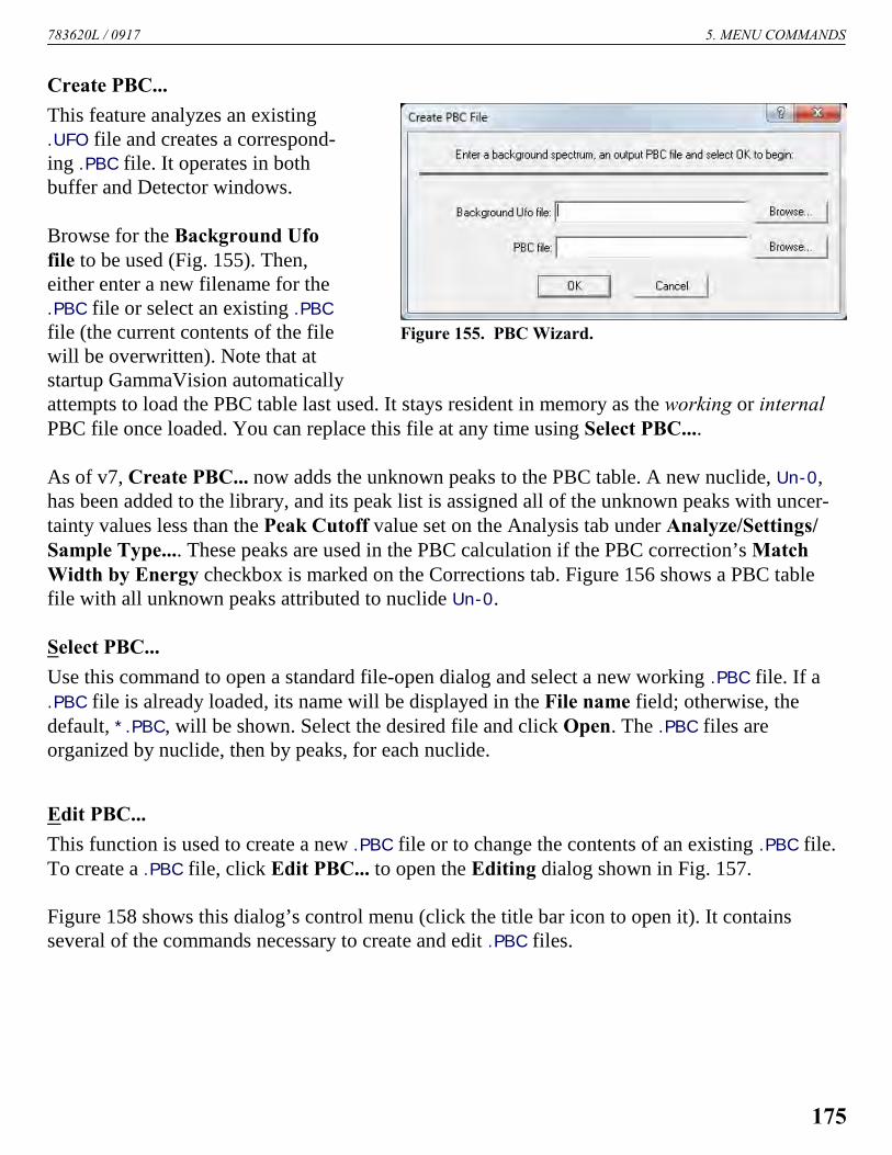
783620L / 0917 5. MENU COMMANDS
Figure 155. PBC Wizard.
Create PBC...
This feature analyzes an existing.UFO file and creates a correspond-ing .PBC file. It operates in bothbuffer and Detector windows.
Browse for the Background Ufofile to be used (Fig. 155). Then,either enter a new filename for the.PBC file or select an existing .PBC
file (the current contents of the filewill be overwritten). Note that atstartup GammaVision automaticallyattempts to load the PBC table last used. It stays resident in memory as the working or internalPBC file once loaded. You can replace this file at any time using Select PBC....
As of v7, Create PBC... now adds the unknown peaks to the PBC table. A new nuclide, Un-0,has been added to the library, and its peak list is assigned all of the unknown peaks with uncer-tainty values less than the Peak Cutoff value set on the Analysis tab under Analyze/Settings/Sample Type.... These peaks are used in the PBC calculation if the PBC correction’s MatchWidth by Energy checkbox is marked on the Corrections tab. Figure 156 shows a PBC tablefile with all unknown peaks attributed to nuclide Un-0.
Select PBC...
Use this command to open a standard file-open dialog and select a new working .PBC file. If a.PBC file is already loaded, its name will be displayed in the File name field; otherwise, thedefault, *.PBC, will be shown. Select the desired file and click Open. The .PBC files areorganized by nuclide, then by peaks, for each nuclide.
Edit PBC...
This function is used to create a new .PBC file or to change the contents of an existing .PBC file.To create a .PBC file, click Edit PBC... to open the Editing dialog shown in Fig. 157.
Figure 158 shows this dialog’s control menu (click the title bar icon to open it). It containsseveral of the commands necessary to create and edit .PBC files.
175

GammaVision® V8 (A66-BW) 783620L / 0917
Figure 156. PBC Table File Displaying Peaks for Nuclide “Un-0.”
Manually Creating a New PBC Table
Open the control menu and click New. This will clear the Edit window so nuclides can beentered manually. Click on the Insert... button to open the dialog shown in Fig. 159. Enter thenuclide name exactly as it appears in the library.
Now, in the peak (right-hand) section of the dialog, click Insert... to open the dialog in Fig. 160.Enter the energy of the gamma ray, the peak activity in cps, and an optional 1-sigma uncertaintybetween 0% and 1000%. The energy must be the same as the library value. Peak energies in thePBC Table and not in the library for this nuclide will not be corrected; likewise for peak energiesin the library and not in the PBC Table for this nuclide.
176

783620L / 0917 5. MENU COMMANDS
Figure 157. PBC Table Editing Dialog.
Figure 158. Edit PBC Dialog ControlMenu.
Figure 159. Edit orManually Add NuclideName.
Figure 160. Edit PBC PeakValues.
Automatically Creating a PBC Table
To make a .PBC file from the background spectrum analysis results (.UFO) file, the backgroundcount rates are extracted from the analysis results file and inserted in a .PBC file. To do this,open the control menu and click on Show Background Analysis.... This will open a standardfile-open dialog. Select the correct .UFO file and click Open. The list of nuclides in the analysiswill be displayed to the left of the PBC Table (see Fig. 161). If no peaks are shown, none were inthe analysis file.
177

GammaVision® V8 (A66-BW) 783620L / 0917
Figure 161. The List of Analysis Nuclides (left) and the PBC Table (right).
Adding Nuclides
There are two Insert buttons at the bottom of the PBC nuclide list: Insert..., which is for man-ually specifying the nuclide; and the button below it, which will be labeled with the name of thenuclide selected in the analysis results list (when no nuclide is selected, this button is labeledInsert Copy).
To automatically add an analysis nuclide to the PBC list: Go to the analysis results list and clickonce on the nuclide of interest. This will activate the gray Insert Copy button at the bottom ofthe PBC list, and change its label to Insert plus the name of the nuclide. Now, in the PBC list,locate the nuclide immediately below the desired insertion position, then click Insert [nuclidename]. This will insert the nuclide, and display the energies and backgrounds for its peaks in theanalysis.
Double-clicking on a nuclide in the analysis results list will insert it into the PBC list immed-iately above the highlighted PBC-list nuclide.
To manually add a nuclide to the PBC list, locate the nuclide immediately below the desiredinsertion position, and click once to highlight it. Next, click the manual Insert... button to openthe dialog shown in Fig. 159, then follow the manual nuclide and peak insertion instructions.
178
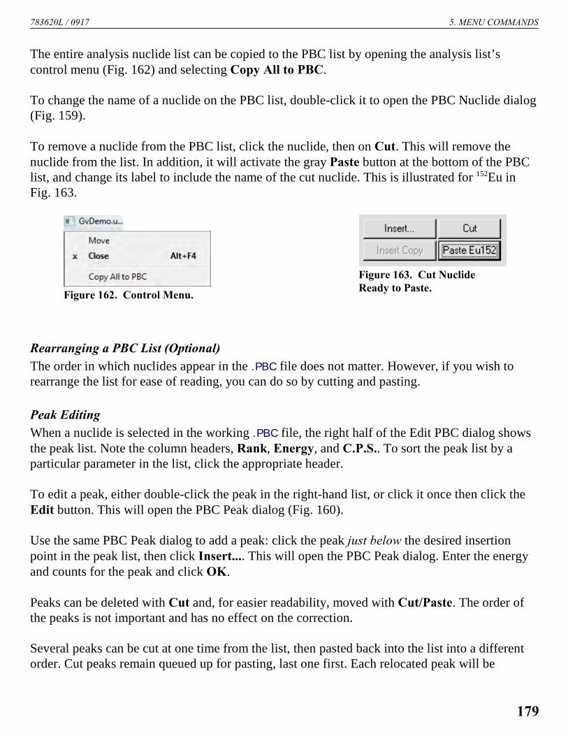
783620L / 0917 5. MENU COMMANDS
Figure 162. Control Menu.
Figure 163. Cut NuclideReady to Paste.
The entire analysis nuclide list can be copied to the PBC list by opening the analysis list’scontrol menu (Fig. 162) and selecting Copy All to PBC.
To change the name of a nuclide on the PBC list, double-click it to open the PBC Nuclide dialog(Fig. 159).
To remove a nuclide from the PBC list, click the nuclide, then on Cut. This will remove thenuclide from the list. In addition, it will activate the gray Paste button at the bottom of the PBClist, and change its label to include the name of the cut nuclide. This is illustrated for 152Eu inFig. 163.
Rearranging a PBC List (Optional)
The order in which nuclides appear in the .PBC file does not matter. However, if you wish torearrange the list for ease of reading, you can do so by cutting and pasting.
Peak Editing
When a nuclide is selected in the working .PBC file, the right half of the Edit PBC dialog showsthe peak list. Note the column headers, Rank, Energy, and C.P.S.. To sort the peak list by aparticular parameter in the list, click the appropriate header.
To edit a peak, either double-click the peak in the right-hand list, or click it once then click theEdit button. This will open the PBC Peak dialog (Fig. 160).
Use the same PBC Peak dialog to add a peak: click the peak just below the desired insertionpoint in the peak list, then click Insert.... This will open the PBC Peak dialog. Enter the energyand counts for the peak and click OK.
Peaks can be deleted with Cut and, for easier readability, moved with Cut/Paste. The order ofthe peaks is not important and has no effect on the correction.
Several peaks can be cut at one time from the list, then pasted back into the list into a differentorder. Cut peaks remain queued up for pasting, last one first. Each relocated peak will be
179
GammaVision® V8 (A66-BW) 783620L / 0917
assigned a Rank number according to its new position. Click the peak just below the desiredinsertion point in the peak list, then click Paste.
Saving or Canceling Changes and Closing the Edit Session
To save this modified .PBC file and use it as the working file, click the control menu, then SavePBC Table As.... Either use the current filename (which will overwrite the previous values) orassign a new filename, then click Save. (GammaVision will assign the default .PBC extension.)To exit the edit session, click the control menu, then Close.
To abandon any changes and restore the .PBC file to its condition before editing, click thecontrol menu, then Close. A dialog will open asking if you want to save the changes; select No.
Print PBC...
Use this command to open a .PBC file and print the PBC table or save it as an ASCII text file,ordered either by Nuclide or Energy. A standard file-open dialog allows you to select thedesired .PBC file, then a printer dialog opens so you may choose a printer or the file-save option.
Figure 164 shows a PBC table saved in both orientations.
5.5.1.6. Average Energy
The Average Energy table is built using the sidebar shown in Fig. 165. The calculation isdescribed in Chapter 6. To make the table, enter the energy per disintegration (keV) and theIsotope name for each isotope to be included in the report. The isotope name must be exactly asgiven in the analysis library.
Now click Enter to create and display the table (see Fig. 166). Each time another isotope isadded, the table updates.
To remove an isotope from the table, click it to select it, then click Delete Isotope on the side-bar. To edit an isotope name or energy, select it with the mouse, make the necessary changes onthe sidebar, and click Enter. The table will update.
To save the current table, click Save.... This opens a file-save dialog. Enter a filename and clickSave; GammaVision will append the default .EBR file extension.
To display an existing table, click Recall..., select the desired file, and click Open.
180

783620L / 0917 5. MENU COMMANDS
Figure 164. PBC Table Ordered by Nuclide (left) and by Energy (right).
181

GammaVision® V8 (A66-BW) 783620L / 0917
Figure 165.
Figure 166. Average Energy Table.
Figure 167. AverageEnergy Sidebar ControlMenu.
Figure 168. Editor Screen for Average Energy Table.
Average Energy Sidebar Control Menu
Figure 167 shows the Average Energy Sidebar’s control menu. To edit an existing file, clickEdit File... and select a file. It will open in a Notepad-like ASCII editor screen (Fig. 168). Theformatting does not have to be exactly as shown. Clicking on Save will save any changes to thefile (in other words, this is not a Save As...).
Destroy clears all values from the current table. Restore abandons any changes and returns thetable to its condition before editing (even after using Destroy), as long as the Restore is exe-cuted before the Average Energy Sidebar is closed. Close closes the sidebar and table, andmakes the currently selected table the internal or working Average Energy table.
182

783620L / 0917 5. MENU COMMANDS
Figure 169. AverageEnergy TableControl Menu.
Figure 170. Iodine EquivalenceSidebar.
Figure 171. Iodine Equivalence Table.
Average Energy Table Control Menu
Figure 169 shows the Average Energy Table control menu. Itcontains commands to Print the table and to Close the table.
5.5.1.7. Iodine Equivalence
The Iodine Equivalence table is built using the sidebar shown inFig. 170. The calculation is described in Section 6.13. To makethe table, enter the Iodine Equivalence and Isotope name foreach isotope to be included in the report. The isotope name mustbe exactly as given in the analysis library.
Now click Enter to create and display the table (see Fig. 171).Each time another isotope is added, the table updates.
To remove an isotope from the table, click it to select it, then click Delete Isotope on the side-bar. To edit an isotope name or energy, select it with the mouse, make the necessary changes onthe sidebar, and click Enter. The table will update.
To save the current table, click Save.... This opens a file-save dialog. Enter a filename and clickSave; GammaVision will append the default .IEQ file extension.
To display an existing table, click Recall..., select the desired file, and click on Open.
183

GammaVision® V8 (A66-BW) 783620L / 0917
Figure 172.
Figure 173. Editor Screen for Iodine Equivalence Table.
Iodine Equivalence Sidebar Control Menu
Figure 172 shows the Iodine Equivalence Sidebar’s control menu. To edit an existing file, clickEdit File... and select a file. It will open in a Notepad-like ASCII editor screen (Fig. 173). Theformatting does not have to be exactly as shown. Clicking on Save will save any changes to thefile (in other words, this is not a Save As...).
Destroy clears all values from the current table. Restore abandons any changes and returns thetable to its condition before editing (even after using Destroy), as long as the Restore is exe-cuted before the Iodine Equivalence Sidebar is closed. Close closes the sidebar and table, andmakes the currently selected table the internal or working Iodine Equivalence table.
Iodine Equivalence Table Control Menu
The Iodine Equivalence Table’s control menu has the same commands as shown in Fig. 169,including the Print command.
5.5.1.8. DAC (MPC)
The DAC (MPC) table is built using the sidebar shown in Fig. 174; the calculation is describedin Section 6.15. To make the table, enter the DAC value (Bq/Kg) and the Isotope name for eachisotope to be included in the report. The isotope name must be exactly as given in the analysislibrary. Now click Enter to create and display the table (see Fig. 175). Each time anotherisotope is added, the table updates.
To remove an isotope from the table, click it to select it, then click Delete Isotope on the side-bar. To edit an isotope name or energy, select it with the mouse, make the necessary changes onthe sidebar, and click Enter. The table will update.
184

783620L / 0917 5. MENU COMMANDS
Figure 174. DAC (MPC) Sidebar.
Figure 175. DAC (MPC) Table.Figure 176. Warning Message.
Figure 177. ConversionFactor.
The DAC units displayed at the top of the sidebar are thecurrently defined analysis units on the Systems tab under Analyze/Settings/Sample Type.... If a .DAC file usingdifferent units is recalled, the dialog in Fig. 176 opens,warning of this difference. Click Yes to open the dialogfor the conversion factor (Fig. 177). Enter the factor andclick OK to scale the table values and put the table inthe analysis units. If No is selected, the analysis and tablewill be in different units and the DAC/MPC calculationwill produce unknown results.
To save the current table, click Save.... This opens a file-save dialog. Enter a filename and click Save; GammaVisionwill append the default .DAC file extension.
To display an existing table, click Recall..., select thedesired file, and click on Open.
DAC (MPC) Sidebar Control Menu
The DAC (MPC) Sidebar contains the same commands as the menuin Figure 172. To edit an existing file, click Edit File... and select a file. It will open in aNotepad-like ASCII editor (Fig. 178). If you make any changes, click Save before closing theeditor window.
Destroy clears all values from the current table. Restore abandons any changes and returns thetable to its condition before editing (even after using Destroy), as long as the Restore is exe-cuted before the DAC (MPC) Sidebar is closed. Close closes the sidebar and table, and makesthe currently selected table the internal or working DAC (MPC) table.
185

GammaVision® V8 (A66-BW) 783620L / 0917
Figure 178. Editor Screen for DAC (MPC) Table.
DAC (MPC) Table Control Menu
The DAC (MPC) Table’s control menu has the same commands as shown in Fig. 169, includingthe Print command.
5.5.1.9. Gamma Total...
As of v6.08, GammaVision supports the EDF’s Gamma Total calculations and report file out-put.2 Figure 179 shows the Gamma Total/EDF Reports Setting dialog. The filenaming conven-tions for the four EDF output file types are discussed on page 188. In addition to these outputfiles you will also be creating .SPC format spectrum files, as discussed below. These will bestored in the location specified for spectra in File/Settings... (Section 5.1.1.4).
Gamma Total analyses can be performed on live spectra or on stored .SPC spectrum files. TheGamma Total setup is saved with the .SPC file. When you recall a spectrum file previously usedfor Gamma Total analysis, the Gamma Total dialog will display the analysis settings in effectwhen the spectrum was saved. These settings can be changed as desired for reanalysis (however,the new settings will not be saved with the spectrum unless you re-save the .SPC file).
NOTE Gamma Total report filenames are keyed to the MCB ID number assigned duringMCB configuration. Before performing these analyses, see the discussion on theassignment of MCB ID numbers on page 11 in Section 2.3.2. If you have more than10 MCBs, or MCBs with the same final digit in their instrument ID, be sure it ispossible to identify which results files correspond to each particular MCB.
186

783620L / 0917 5. MENU COMMANDS
Each analysis produces one or more characteristic output files, as discussed in the followingsection. In addition, an EDF Special Applications Report section is added to the end of thestandard GammaVision report (see Section 7.8). This table lists the Gamma Total settings usedin the analysis, and the quantitative results. If the EDF Table Only box is marked, the standardreport contains only the header information and the EDF Special Applications Report table.Otherwise, the EDF table is included on the standard report, along with the other report optionsspecified on the Report tab under Analyze/Settings/Sample Type... (page 156).
To turn off the EDF table in the GammaVision report, unmark all reporting options before thenext analysis.
Gamma Total analyses are typically predicated on an energy range of 100 keV to 2 MeV. If youuse a different energy range, you might wish to adjust the Integration Range on the GammaTotal dialog accordingly.
Figure 179. Gamma Total Setup Dialog Configured for GammaTotal Reporting.
187

GammaVision® V8 (A66-BW) 783620L / 0917
Output File Naming Convention
Background Report File
The background report file is named according to:
B#ddmmyy.XXX
where # is the last digit of the instrument ID number as assigned by the MCB Configurationprogram; and ddmmyy is the analysis date as two-digit date, two-digit month, and the lasttwo digits of the year.
Analysis Report File
Analysis report files, for gamma total and germanium reporting, are named according to:
#_ddmmyy.Seq
where # is the last digit of the instrument ID number as assigned by the MCB Configurationprogram; ddmmyy is the analysis date as two-digit date, two-digit month, and the last twodigits of the year; and Seq is the spectrum sequence number, as determined by the entry inthe Gamma Total Sequence and Germanium Sequence fields on the Gamma Total dialog.
Germanium Results File
The germanium reporting file is named according to:
DETAIL.Seq
where Seq is the spectrum sequence number, as determined by the entry in the GermaniumSequence field on the Gamma Total dialog.
Maintenance Report File
These files, for cesium reporting, are named according to:
RDTCS_#.XXX
where # is the last digit of the instrument ID number.
Hardware and Analysis Configuration
Before acquiring data for a Gamma Total analysis, prepare the system as follows:
! The detector must be energy and efficiency calibrated.
188

783620L / 0917 5. MENU COMMANDS
! Select Analyze/Settings/Sample Type... and configure the analysis settings according toyour site procedures.
! Use Acquire/MCB Properties... to set the presets and other hardware properties.
Configuring and Generating the Gamma Total Reports
Background Counting Procedure
On the Gamma Total dialog, mark only the Count Background checkbox (unmark anyGamma Total options in the left column, if they are marked). This procedure auto-generatesa background report, so there is no need to mark the Write Background Report checkbox.
Select the location for the Gamma Total Report Dir. The background file will be written tothis folder.
Remove any entries from the Background Spectrum, Cesium Spectrum, and GeometryFile fields, and click OK.
Count, analyze with Analyze/Entire spectrum in memory..., and save the resultingbackground spectrum for use in other Gamma Total analyses. This will generate a GammaTotal background file, B#ddmmyy.XXX, in addition to the background .SPC file.
Cesium Counting Procedure
On the Gamma Total dialog, mark only the Count Cs-137 checkbox (unmark any GammaTotal or background options, if they are marked). This selection auto-generates amaintenance report so there is no need to mark the Write Maintenance Report checkbox.
Select the location for the Gamma Total Report Dir. The maintenance file will be writtento this folder.
Browse for a Background Spectrum; then select the Geometry File location and enter anew or existing geometry filename. Click OK.
Count, analyze with Analyze/Entire spectrum in memory..., and save the resulting cesiumspectrum for use in Gamma Total Reporting analyses. This will generate a Gamma Totalmaintenance file, RDTCS_#.XXX, and a geometry file with a user-assigned filename and a.TXT extension, in addition to the cesium .SPC file.
189

GammaVision® V8 (A66-BW) 783620L / 0917
Gamma Total Counting ProcedureOn the Gamma Total dialog, mark the Enable Gamma Total Reporting checkbox (makesure Count Background and Count Cs-137 are unmarked). This will automatically markthe Enable Gamma Total Calculation and EDF Table Only boxes.
Select the location for the Gamma Total Report Dir.
Browse for a Background Spectrum; then select the Geometry File location and enter anexisting geometry filename. Click OK.
If Write Background Report is checked, a background report will be generated. If you alsospecify a cesium spectrum, the K-factor to be used in the Gamma Total activity calculationwill be calculated from the cesium and background spectra. If the geometry file is specifiedas well, then the K-factor calculated on-the-fly will be saved to the geometry file (instead ofreading the K-factor from the geometry file). In addition, if the cesium spectrum is specifiedand Write Maintenance File is marked, a maintenance file will be generated.
Count, analyze with Analyze/Entire spectrum in memory..., and save the resulting spec-trum. This will generate a Gamma Total analysis file #_ddmmyy.Seq, in addition to theGamma Total .SPC file.
To count only the background within the Integration Range when performing backgroundQA measurements (Section 8.2.2), mark the Use Range for Background QA checkbox inthe bottom section of the dialog.
Germanium Counting ProcedureOn the Gamma Total dialog, mark only the Enable Germanium Reporting checkbox(unmark any other reporting selections except, optionally, Report ISO NORM MDA OnReports, as described below.).
Select the location for the Gamma Total Report Dir and the Germanium Report Dir.
No entries are required in the Background Spectrum, Cesium Spectrum, and GeometryFile fields. However if you want a background report generated, mark the Write Back-ground Report field and recall a Background Spectrum. If you also specify a cesium spec-trum, the K-factor to be used in the Gamma Total activity calculation will be calculated fromthe cesium and background spectra. If a geometry file is specified as well, then the K-factorcalculated on-the-fly will be saved to the geometry file (instead of reading the K-factor fromthe geometry file). If you want a maintenance file generated, mark Write Maintenance Fileand include a cesium spectrum.
190

783620L / 0917 5. MENU COMMANDS
Figure 180. Generate an ROI Report.
To save the ISO NORM MDA values, instead of the regular MDA values, to the germaniumresults file, mark the Report ISO NORM MDA On Reports checkbox.
NOTE To enable this checkbox, you must first mark the ISO NORM checkbox on theReport tab under Analyze/Settings/Sample Type....
Count, analyze with Analyze/Entire spectrum in memory..., and save the resulting spec-trum. This will generate a Gamma Total analysis file #_ddmmyy.Seq, and a germaniumresults file DETAIL.Seq, in addition to the germanium .SPC file.
To count only the background within the Integration Range when performing backgroundQA measurements (Section 8.2.2), mark the Use Range for Background QA checkbox inthe bottom section of the dialog.
5.5.2. Peak Search
This command initiates a Mariscotti27-type peak search on the spectrum. The peak-search sensi-tivity is selected on the Systems tab of the Sample Type Settings dialog (see the discussionbeginning on page 152). Each peak found is marked with an ROI. If the system is calibrated, thewidth of the ROI is three times the calculated FWHM of the peak. If not calibrated, the width ofthe ROI is based on the width of the peak as determined by the peak search. Overlapping orclose peaks might have contiguous ROIs. Existing ROIs are not cleared.
The report function can be used with Peak Search to produce a semi-quantitative nuclide list forthe spectrum.
5.5.3. ROI Report...
The ROI Report... function creates areport describing acquisition conditionsand contents of all ROIs, and sends itto a disk file, the display, or the printer.The dialog shown in Fig. 180 can directthe report output to a disk file (namechosen by user), a printer, or the screen.
27M.A. Mariscotti, “A Method for Automatic Identification of Peaks in the Presence of Background and itsApplication to Spectrum Analysis,” Nuclear Instruments and Methods 50, 309!320 (1967).
191

GammaVision® V8 (A66-BW) 783620L / 0917
Detector # 1 ACQ 30-Sep-91 at 14:47:00 RT = 250057.0 LT = 250000.0
No detector description was entered Background in shield with copper liner
ROI # 1 RANGE: 297 = 63.26keV to 323 = 67.86keV AREA : Gross = 4231 Net = 490 +/-116 CENTROID: 309.50 = 65.47keV SHAPE: FWHM = 0.96 FW(1/10)M = 2.11 No close library match.
ROI # 2 RANGE: 708 = 135.95keV to 736 = 140.91keV AREA : Gross = 5898 Net = 482 +/-145 CENTROID: 724.08 = 138.80keV SHAPE: FWHM = 0.66 FW(1/10)M = 1.40 ID: Hf181 at 136.28keV Corrected Rate = 0.76 +/- 0.23 Bq
Detector # 1 ACQ 30-Sep-91 at 14:47:00 RT = 250057.0 LT = 250000.0 No detector description was entered Background in shield with copper liner
Figure 181. Example of Paragraph-Format Report.
Only the ROIs in the expanded view are shown on the display. You can also select from tworeport formats, Paragraph and Column.
Examples of the Paragraph and Column format are illustrated in Figs. 181 and 182, respec-tively. The information supplied is the same in both formats.
If the spectrum is not calibrated, the following are reported for each ROI:
! ROI number! Start channel of the ROI! Stop channel of the ROI! Gross area of the peak! Net area of the peak, as calculated in Calculate/Peak Info! Error in net area, as calculated in Calculate/Peak Info! Centroid channel of peak, as calculated in Calculate/Peak Info! FWHM! FW(1/x)M
192
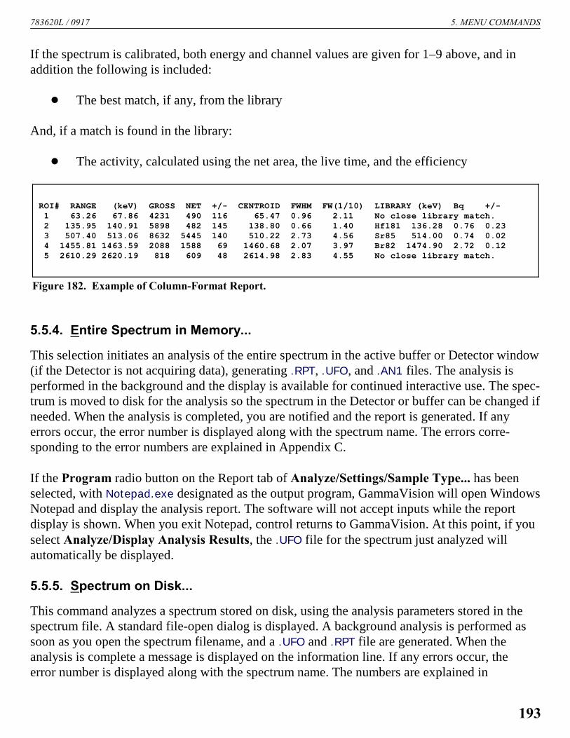
783620L / 0917 5. MENU COMMANDS
ROI# RANGE (keV) GROSS NET +/- CENTROID FWHM FW(1/10) LIBRARY (keV) Bq +/- 1 63.26 67.86 4231 490 116 65.47 0.96 2.11 No close library match. 2 135.95 140.91 5898 482 145 138.80 0.66 1.40 Hf181 136.28 0.76 0.23 3 507.40 513.06 8632 5445 140 510.22 2.73 4.56 Sr85 514.00 0.74 0.02 4 1455.81 1463.59 2088 1588 69 1460.68 2.07 3.97 Br82 1474.90 2.72 0.12 5 2610.29 2620.19 818 609 48 2614.98 2.83 4.55 No close library match.
Figure 182. Example of Column-Format Report.
If the spectrum is calibrated, both energy and channel values are given for 1–9 above, and inaddition the following is included:
! The best match, if any, from the library
And, if a match is found in the library:
! The activity, calculated using the net area, the live time, and the efficiency
5.5.4. Entire Spectrum in Memory...
This selection initiates an analysis of the entire spectrum in the active buffer or Detector window(if the Detector is not acquiring data), generating .RPT, .UFO, and .AN1 files. The analysis isperformed in the background and the display is available for continued interactive use. The spec-trum is moved to disk for the analysis so the spectrum in the Detector or buffer can be changed ifneeded. When the analysis is completed, you are notified and the report is generated. If anyerrors occur, the error number is displayed along with the spectrum name. The errors corre-sponding to the error numbers are explained in Appendix C.
If the Program radio button on the Report tab of Analyze/Settings/Sample Type... has beenselected, with Notepad.exe designated as the output program, GammaVision will open WindowsNotepad and display the analysis report. The software will not accept inputs while the reportdisplay is shown. When you exit Notepad, control returns to GammaVision. At this point, if youselect Analyze/Display Analysis Results, the .UFO file for the spectrum just analyzed willautomatically be displayed.
5.5.5. Spectrum on Disk...
This command analyzes a spectrum stored on disk, using the analysis parameters stored in thespectrum file. A standard file-open dialog is displayed. A background analysis is performed assoon as you open the spectrum filename, and a .UFO and .RPT file are generated. When theanalysis is complete a message is displayed on the information line. If any errors occur, theerror number is displayed along with the spectrum name. The numbers are explained in
193

GammaVision® V8 (A66-BW) 783620L / 0917
Figure 183. Display from .UFO File.
Appendix C.
If the Program radio button on the Report tab of Analyze/Settings/Sample Type... has beenselected, with Notepad.exe designated as the output program, GammaVision will open WindowsNotepad and display the analysis report. Close Notepad to end the analysis session and return toGammaVision.
5.5.6. Display Analysis Results...
This command displays the results of an analysis of the complete spectrum by reading the resultsstored in a .UFO file(Fig. 183).28
28.UFO files are created by any analysis command, including Entire spectrum in memory and Spectrum fromdisk on the Analyze menu, and Start/Save/Report on the Acquire menu.
194

783620L / 0917 5. MENU COMMANDS
Figure 184. Analysis ResultsSidebar.
This analysis considers all of the spectrum and all library entries, thus differing from the inter-active analysis results. When you select Display analysis results, the .UFO file matching theactive spectrum’s filename will be highlighted and ready to open; just click OK. To compare theanalysis results to the corresponding spectrum, the spectrum analyzed should first be recalledinto a buffer window.
5.5.6.1. Analysis Sidebar
Figure 184 shows the Analysis Sidebar. The buttons move the marker up and down through theresults list, library, and spectrum simultaneously.
The within Nuclide buttons move up and down the library list for the selectednuclide, in the order the energies are stored in the library. Since the libraryenergies are not usually stored in increasing energy order, this will cause themarker to jump about the spectrum. This is useful in deciding if a nuclide ispresent or not, by looking for all the lines associated with the nuclide. If theselected peak has a zero area, it is not displayed.
The Energy buttons move the cursor up and down throughthe library peak list in energy order. Only non-zero-areapeaks are shown. Since the library used for the analysismight not be the same as the working library, this might bea different set of peaks than found with the Library buttonson the Status Sidebar.
The Peak buttons move the marker up and down throughall the peaks in the spectrum. This includes non-zero-arealibrary peaks and unknown peaks above the peak-searchsensitivity cutoff.
The Unk nown buttons move the marker up and downthrough the unknown peaks that satisfy the sensitivity cutoff, in energy order,skipping over any library peaks.
The Multiplet buttons move up and down through the multiplet or deconvolutedregions in the spectrum. The multiplet up button goes to the first (lowest-energy)peak of the next higher multiplet. Similarly, the multiplet down button goes tothe last (highest-energy) peak of the next lower multiplet. To look at individualpeaks in the multiplet, use the Peak, Energy, or Unknown buttons.
195

GammaVision® V8 (A66-BW) 783620L / 0917
Figure 185. Spectrum ResidualsDisplay (arrow).
Figure 186. AnalysisResults SpectrumWindow Menu (right-click to open).
The ROI, Peak, and Library buttons on the StatusSidebar are also active.
Marking the Show Residuals check box adds a linebeneath the spectrum that displays the differencebetween the actual spectrum and the calculatedspectrum based on the analysis and the calibrationpeak shape. An example is shown in Fig. 185.
5.5.6.2. Analysis Results Spectrum Window
This release of GammaVision features an improvedAnalysis Results Spectrum Window that gives youmore flexibility in displaying and printing your analy-sis results. Right-clicking in the spectrum windowopens the right-mouse-button menu shown in Fig. 186.
Plot Absolute Residuals/Plot Relative Residuals
These commands are active if the Show Residuals checkbox is marked on the analysis sidebar. The residuals area comparison of the counts in each channel (Actual) to thecalculated counts for that channel as determined by thepeak-fitting algorithm (Fitted). Plot Absolute Residualsdisplays the difference in each channel, in counts, betweenActual and Fitted counts. Plot Relative Residuals displaysthe difference in each channel, in standard deviations(abbreviated STD on the screen), between Actual and Fittedcounts divided by the square root of the Actual counts; thatis, .
The Properties command allows you to modify the screencolors and y-axis scaling for the residuals histogram.
Zoom In
Zoom In adjusts the horizontal and vertical scales in theExpanded Spectrum Window to view a smaller portion ofthe spectrum. This command is duplicated by the Zoom Inbutton on the toolbar.
196

783620L / 0917 5. MENU COMMANDS
Figure 187. Inactive(solid) and Active(diagonal fill) ROI Bars.
Zoom Out
Zoom Out adjusts the horizontal and vertical scales in the Expanded Spectrum Window to viewa larger portion of the spectrum. This command is duplicated by the Zoom Out button on thetoolbar.
Undo Zoom In
This will undo or reverse the last Zoom In operation done with the rubber rectangle. It restoresthe display to the horizontal and vertical expansion before the Zoom In. It is not the same asZoom Out.
Full View
Full View adjusts the horizontal and vertical scaling to display the entire spectrum in theExpanded Spectrum View.
Mark ROI
This allows you to mark a peak as an ROI by clicking and dragging the rubber rectangle across aportion of the spectrum, then selecting Mark ROI. If Show ROI Bars is on, the new ROI willbe marked with the active ROI Bars until you either move to or create another ROI.
Clear Active ROI
This clears the ROI bits in all ROI channels that adjoin the channel containing the marker.
Show ROI Bars
These are vertical markers that indicate the lower and upperboundaries of each ROI in the spectrum. The ROI bars foran inactive/unselected ROI have solid fill; when you click anROI to activate it (only one is active at a time), the bars for theactive ROI change to a diagonal fill (see Fig. 187). To displaythe ROI bars, right-click in the expanded window to open theright-mouse-button menu, then click ROI Bars to checkmarkit. To hide the ROI bars, click the command again to clear thecheckmark.
197

GammaVision® V8 (A66-BW) 783620L / 0917
Figure 188. The Peak Info Window for anROI.
When you activate an ROI by clicking on it, the low (start) and high (end) positions marked bythe ROI bars are displayed on the Marker Information Line.
You can shift the start and end channels of an ROI by clicking and dragging the ROI bars (allowa moment for the display to update).
The ROI bar color is controlled by the Markers droplist in the Graph Properties dialog.
Peak Info
This command opens a Peak Info box(Fig. 188) for the selected peak and leaves thebox open until you click inside it. This com-mand works for peaks loaded from a .UFO file,and ROIs created within GVPlot or loaded froman .ROI file. The contents of the Peak Info boxare described in Section 5.4.3. You can simul-taneously display multiple Peak Info boxes aslong as they do not overlap. A new Peak Infobox will close any existing boxes that it overlaps.For very narrow peaks, you might find it usefulto position the marker with the left/right arrowkeys before calling the Peak Info command.When the marker is on a peak, the right sideof the Marker Information Line will display aPeak Area readout.
Show Hover Window
When you select this command, a checkmark is displayed by this menu item to indicate that it isin hover-window mode. In this mode, the Peak Info window opens when the mouse pointer ispaused over a peak for approximately 1 second, and closes when the pointer is moved away fromthe peak. To turn off hover mode, select Show Hover Window again to remove the checkmark.This mode can be used together with Peak Info.
Sum Spectrum
This sums the gross counts in the area selected with the rubber rectangle or, if you have notselected an area, the gross counts in the entire spectrum. The results are displayed on the statusline, and indicate the span of channels summed.
198

783620L / 0917 5. MENU COMMANDS
Figure 189. Customize Graph Styling.
Print Graph
This command prints the Analysis Results Spectrum Window. It duplicates File/Save Plot.
Properties
This opens the Graph Properties dialog(Fig. 189), which lets you set the graphcolors, symbol type, and axis scalingfactors. All settings are reset when youexit GammaVision.
The Text color affects the color of theaxes, axis labels, and spectrum title.Background controls the color of thespectrum background. Markers appliesto the ROI bars, and nuclide labels andpointers.
Data Set Colors allows you to chooseseparate colors for spectrum Data, Fit-ted peaks, and Residuals; select a datatype from the left-hand droplist, thenchoose a color from the list on the right. Similarly, use Fill Color to control the colors of ROIs,Nuclide Peaks, Unknown Peaks, Multiplets, and Composites. Spectrum Style determineshow the histogram data are represented (Points, Line, or Fill All).
The Show Nuclide Name checkbox allows you to hide or display the nuclide markers for ananalyzed spectrum. Clearing the Show Axes checkbox removes the axes so the histogramoccupies the entire window without an inside border.
Set the Y Axis Scale of the spectrum window to Linear or Logarithmic. You can also do thiswith the LOG button on the toolbar except as noted in the bullet list below.
The Draw Multiplet radio buttons determine whether multiplets are drawn as a Compositecurve, shown individually (Each), or displayed as individual peaks superimposed with the com-posite curve (Both). These modes are compared in Fig. 190. This display is most easily seenwith all Fill Modes turned off (checkboxes unmarked).
The Fill Mode checkboxes allow you to determine which peak types, if any, will be displayed infill mode rather than data-point mode.
199

GammaVision® V8 (A66-BW) 783620L / 0917
Figure 190. Draw Multiplet Modes.
The toolbar’s Auto button is interlocked with theAuto Y (Spectrum) checkbox. Therefore, clickingthe toolbar’s Auto button on and off respectivelyturns on and off the Auto Y (Spectrum) feature inthe analysis results Graph Properties dialog, andvice versa.
Similarly, the LOG button on the toolbar is inter-locked with the Linear and Log radio buttons in theY Axis Scale section of the Graph Properties dialog.
The y-axis in the Display Analysis Results windowis referred to as being in auto mode when (1) theAuto Y (Spectrum) checkbox is marked or (2) theAuto Y (Spectrum) box is unmarked and the rangeis set from 0 to 0. In auto mode, the LOG and Auto toolbar buttons behave as they do in theregular Detector and buffer windows.
When the Auto Y (Spectrum) checkbox is unmarked and the range is other than 0 to 0, they-axis is referred to as being in manual range mode. When the y-axis is in manual range mode,the LOG and Auto buttons behave as follows:
! The LOG button toggles the y-axis between logarithmic (on) and linear (off) scaling.
! The Auto button toggles the y-axis between the auto (on) and manual (off) ranges.
! The LOG and Auto buttons work independently. They can both be turned on at the sametime to achieve an Auto range with a logarithmic scale.
NOTE Manually setting the range for one axis disables zooming for that axis only. If both axisranges are manually fixed, all zooming is disabled.
5.5.6.3. Analysis Results Table
Figure 191 shows the Analysis Results Table window. The table records can be sorted by anyparameter (e.g., energy, area, nuclide, FWHM) by clicking on the desired column header.
The Analysis Sidebar’s control menu is shown in Fig. 192 (click the title bar icon to open themenu). Mark or unmark Table to show or hide the Analysis Results Table; use Print on theAnalysis Results Table control menu to print the table as displayed (note that this is not the sameas the complete report described in Chapter 7).
200

783620L / 0917 5. MENU COMMANDS
Figure 191. Analysis Results Table.
Figure 192.
Figure 193. Details of Analyzed Peak Derived from the .UFO File.
When the Analysis Results Table is displayed and GammaVision is ininteractive-analysis mode, you can see more details about any peak bydouble-clicking on that peak in the table. This opens a Details window,as shown in Fig. 193. Use the Peak buttons to step to the next-highest-energy and next-lowest-energy peaks. Click Close or press <Esc> toexit.
201

GammaVision® V8 (A66-BW) 783620L / 0917
The Details window shows the following peak information, derived from the .UFO file structure(which is described in detail in the File Structure Manual):
Peak energyThe library peak energy in keV, or the centroid energy for unknown peaks.
Peak centroidThe peak centroid energy from the spectrum.
Peak centerThe peak centroid channel from the spectrum.
Peak range of integrationThe low and high channel numbers for the peak region. These are the beginning and endchannel numbers for the background region around a single peak. See also Multiplet rangeof integration.
Multiplet range of integrationThe low and high channel numbers for the multiplet region. These are the beginning and endchannel numbers for the background region around the entire multiplet. All peaks in themultiplet will have the same low-/high-channel values.
Full-width-1/2-maximumThe full width at half maximum of the peak. It is a measured value for single peaks and acalculated value for peaks in a multiplet region.
Full-width-1/10-maximumThe full width at tenth maximum of the peak. It is a measured value for single peaks and acalculated value for peaks in a multiplet region.
Full-width-1/25-maximumThe full width at twenty-fifth maximum of the peak. It is a measured value for single peaksand a calculated value for peaks in a multiplet region.
Gammas per 100 disintegrationsBranching ratio from library, if peak was identified.
Net areaThe corrected net area of the peak. For example, the PBC correction could be applied to thisnumber.
202

783620L / 0917 5. MENU COMMANDS
BackgroundThe corrected peak background calculated by the program.
Counting uncertaintyThe 1-sigma counting uncertainty in the peak net area, as a fraction.
Isotopic abundanceThe activity for this nuclide based on this peak only. It is zero for unknown peaks or if thereis no efficiency calibration.
MDAThe minimum detectable activity for this nuclide based on this peak only. It is zero forunknown peaks or if there is no efficiency calibration.
Width of background region below peakWidth of background region above peak
The number of channels used in the calculation of the background below and above the peak(as selected on the Sample tab under Analyze/Settings/Sample Type...). If the backgroundselection is set to a given number, then these will both be the same. For the Auto backgroundsetting, these can be different.
Average background below peakAverage background above peak
TCC flagWas TCC enabled?
Original branching ratio of TCC peakOriginal branching ratio if TCC was enabled
Suspect library nuclideSuspect library nuclide name, if peak was not identified.
Second MDA valueIf a second MDA calculation is specified in the b30winds.ini (n30winds.ini for NAI32) file,this is the second MDA value. Otherwise, the value is zero.
5.5.7. Interactive in Viewed Area...
Interactive in viewed area... starts an interactive analysis session by analyzing the spectrumnow displayed. This command is active only when the Expanded Spectrum View displays #4096channels (zoom in on a portion of the spectrum to activate this command). The working library
203

GammaVision® V8 (A66-BW) 783620L / 0917
Figure 194. Results Interactive in Viewed Area.
selected with Library/Select File... is used. The analysis parameters have been set in theAnalyze/Settings/Sample Type... dialogs. When the analysis is complete, the graphical resultsand peak area table are displayed as illustrated in Fig. 194. The table records can be sorted bysuch parameters as energy, area, FWHM, and background by clicking on the desired columnheader.
NOTE This interactive method uses a different analysis engine than the one specified in theSample Defaults (Analyze/Settings/Sample Type...), therefore, results from the twoengines might differ somewhat. To see the analysis results generated by the SampleDefaults, use Display Analysis Results... instead of the interactive function.
204

783620L / 0917 5. MENU COMMANDS
Figure 195 shows the interactive Analysis Sidebar. The buttons move the marker up and downthrough the results lists, library, and spectrum simultaneously.
The buttons in the Library Peak section pertain to the results from the analysis; the other but-tons pertain to the spectrum. The peak-found buttons move to the next higher or lower peak inthe analysis results list. This includes non-zero-area library and unknown peaks above the cutoff.See Peak button below.
The within Nuclide buttons move up and down thelibrary list for the selected nuclide, in the order theenergies are stored in the library. Since the libraryenergies are not usually stored in increasing energyorder, this will jump the marker around in the spec-trum. This is useful in deciding if a nuclide is presentor not, by looking for all the lines associated with thenuclide. Only non-zero-area peaks are displayed.
The Energy buttons move the marker up and downthrough the library peak list in energy order. Onlynonzero-area peaks are shown. Since the library usedfor the analysis might not be the same as the work-ing library, this might be a different set of peaksthan found with the Peak buttons.
The Peak buttons move up and down through thepeaks found by the online peak search. (The sensitivity is set in the systemsettings.) This might select more peaks than the analysis peaks above becauseof the difference in the cut-off. If the sensitivity for analysis is low, e.g., 5%,many peaks will not be reported because their uncertainty is too high. Theywill have been found by the analysis, but not reported.
The Unknown buttons move the marker up and down through the unknownpeaks in energy order, skipping over any library peaks. Only peaks thatsatisfy the sensitivity cutoff are shown. Note that the Library Peak andUnknown buttons select different groups of peaks.
The Multiplet buttons move up and down through the multiplet or deconvo-luted regions in the spectrum. The next time the multiplet up button isclicked, the marker goes to the first (lowest-energy) peak of the next-highermultiplet. The next down button goes to the last (highest-energy) peak of the
Figure 195. Analysis DisplayControls.
205
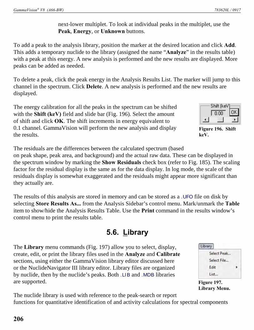
GammaVision® V8 (A66-BW) 783620L / 0917
Figure 196. ShiftkeV.
Figure 197. Library Menu.
next-lower multiplet. To look at individual peaks in the multiplet, use thePeak, Energy, or Unknown buttons.
To add a peak to the analysis library, position the marker at the desired location and click Add.This adds a temporary nuclide to the library (assigned the name “Analyze” in the results table)with a peak at this energy. A new analysis is performed and the new results are displayed. Morepeaks can be added as needed.
To delete a peak, click the peak energy in the Analysis Results List. The marker will jump to thischannel in the spectrum. Click Delete. A new analysis is performed and the new results aredisplayed.
The energy calibration for all the peaks in the spectrum can be shiftedwith the Shift (keV) field and slide bar (Fig. 196). Select the amountof shift and click OK. The shift increments in energy equivalent to0.1 channel. GammaVision will perform the new analysis and displaythe results.
The residuals are the differences between the calculated spectrum (basedon peak shape, peak area, and background) and the actual raw data. These can be displayed inthe spectrum window by marking the Show Residuals check box (refer to Fig. 185). The scalingfactor for the residual display is the same as for the data display. In log mode, the scale of theresiduals display is somewhat exaggerated and the residuals might appear more significant thanthey actually are.
The results of this analysis are stored in memory and can be stored as a .UFO file on disk byselecting Store Results As... from the Analysis Sidebar’s control menu. Mark/unmark the Tableitem to show/hide the Analysis Results Table. Use the Print command in the results window’scontrol menu to print the results table.
5.6. Library
The Library menu commands (Fig. 197) allow you to select, display,create, edit, or print the library files used in the Analyze and Calibratesections, using either the GammaVision library editor discussed hereor the NuclideNavigator III library editor. Library files are organizedby nuclide, then by the nuclide’s peaks. Both .LIB and .MDB librariesare supported.
The nuclide library is used with reference to the peak-search or reportfunctions for quantitative identification of and activity calculations for spectral components
206

783620L / 0917 5. MENU COMMANDS
Figure 198. Peak List Dialog Box.
according to calibrated peak energy. The nuclide library data include the nuclide name, half-life,and half-life uncertainty. The nuclide names can be any combination of eight characters, butmust be consistent throughout all files. The library peak data include the energies and branchingratio or gammas/disintegration for each energy.
At startup, GammaVision automatically attempts to load the library last loaded (the first timeyou run GammaVision, the library DEFAULT.LIB is used). Thereafter, this working library can bereplaced at any time with Library/Select File.... The library stays resident in memory after it hasbeen loaded.
In the analysis report, the nuclides are listed in the order they are in the library. The size of aworking library is limited to 65,000 bytes for any combination of nuclides and peaks (e.g., about100 nuclides with 1900 peaks or 200 nuclides with 1600 peaks). Master or reference libraries(e.g., MASTER.LIB from A53-BI or MASTER.MDB from NuclideNavigator), from which the work-ing libraries are built, can be any size. To analyze using larger libraries, such as those created byNuclideNavigator III, the library for the analysis is specified in Analyze/Settings/SampleType... as the library from disk.
NOTE Some old libraries might need to be rebuilt by copying the complete library to a newlibrary with the Library/Edit... feature (Section 5.6.3). The “Can’t read library”error means this should be done.
5.6.1. Select Peak...
This opens a window containing a list of thelibrary peaks in energy order (Fig. 198). Thislist shows the nuclide name, energy, gammas/100 disintegrations, and half life. Clickingon any field moves the marker line to thatenergy in the spectrum.
The Library List can be sorted by nuclide,energy, percent, or half life by clicking onthe desired column header.
5.6.2. Select File...
This opens the Load Library File dialog(Fig. 199). If a library has already been selected,it is shown in the File name field. If File namecontains a generic entry of *.LIB or *.MDB, nolibrary is currently selected. Select the desired
207

GammaVision® V8 (A66-BW) 783620L / 0917
Figure 199. Select an .LIB- or .MDB-Format Library File.
disk and filename and click Open. This library becomes the working library.
5.6.3. Edit...
Use this command to create a new library file or change the contents of an existing library file. Itallows you to select the GammaVision Editor... or Nuclide Navigator... (if NuclideNavigatorIII is installed). The GammaVision library editor is discussed here. The NuclideNavigator editoris described in the NuclideNavigator III user manual.
Figure 200 shows the GammaVision library Editing dialog.
The control menu (click the title bar icon to open it) is shown in Fig. 201. It contains several ofthe commands necessary to create, edit, and print the .LIB files.
208

783620L / 0917 5. MENU COMMANDS
Figure 200. Editing Library Dialog.
Figure 201. Library EditDialog Control Menu.
5.6.3.1. Copying Nuclides From Library to Library
To copy nuclides from one library to another library — for example, to make a working libraryfrom a master library — click on the Edit window’s control menu and select Show MasterLibrary. This will open a file selection dialog. Choose the desired disk and file and click Open.Both libraries will be displayed side by side, as illustrated in Fig. 202.
209

GammaVision® V8 (A66-BW) 783620L / 0917
Figure 202. The Master Library (left) and Library Editing Dialog (right).
Figure 203. Add a Nuclide.
To copy a nuclide from the master library to theworking library: Go to the master library list andclick once on the nuclide of interest. This will acti-vate the gray Insert Copy button at the bottom of theEditing dialog’s nuclide list, and change its label toInsert plus the name of the nuclide. Now, in the Edit-ing dialog, locate the nuclide immediately below thedesired insertion position, click it once, then clickInsert [nuclide name]. This will insert the nuclideand display its peak list on the right.
Double-clicking on a nuclide in the master librarywill add it to the working library, inserting it imme-diately above the currently highlighted nuclide inthe list.
5.6.3.2. Creating a New Library Manually
Open the control menu and click New. This will clear the Editing dialog so nuclides can beentered manually. Click the Insert... button to open the Insert Library Nuclide dialog, shown inFig. 203. Enter the Nuclide Name and Half Life and click OK.
210

783620L / 0917 5. MENU COMMANDS
Figure 204. Readyto Edit this Nuclide.
Figure 205. Edit or Manually AddNuclide Name.
NOTE We recommend that you enter the standard name for the nuclide so that Nuclide Navi-gator will be able to recognize it. If you use a non-standard name, the TCC calculationscould fail due to an inability to compute the parent daughter relationships.
Click the desired row under the Rank/Energy/Percent heading to highlight that row. Now, atthe bottom of the (right-hand) peak list, click Insert... to open the Edit Library Peak dialog(Fig. 207). Enter the energy of the gamma ray and the branching ratio of the peak.
5.6.3.3. Editing Library List Nuclides
To edit the information about a nuclide in the working library:
Click the nuclide to highlight it. The Edit... button (in the upperright of Fig. 200) will change to Edit plus the name of the nuclide,as shown in Figure 204.
Click Edit [nuclide].... This will open the Edit Library Nuclide dialog(Fig. 205). The Nuclide Name, Half Life, Uncertainty, and Nuclide Flags will already belisted.
The Uncertainty is a single number that represents theoverall uncertainty (2 sigma or 95% confidence level)in the branching ratios entered for this nuclide. The1-sigma uncertainty is added in quadrature to form thetotal uncertainty on the final report. The Uncertaintyvalue should be taken from the nuclear data sheet forthis nuclide. The default is 5%, but 2% is a realisticnumber.
The first six Nuclide Flags are used to show how thenuclide was produced. For example, Thermal NeutronActivation (T) indicates that this nuclide is producedwhen the parent nuclide absorbs a slow neutron. Thiscan be helpful in organizing reports by nuclide category.More than one flag can be checked. Libraries producedwith Nuclide Navigator II or later versions will alreadyhave these flags set. For other libraries, it will be neces-sary to consult a reference for the proper settings.
The No MDA Calculation flag indicates that the nuclide will not be reported unless present inthe spectrum. If this is not marked, the MDA value will be printed if the nuclide is not present inthe spectrum.
211

GammaVision® V8 (A66-BW) 783620L / 0917
Figure 206. Cut Nuclide isReady to Paste.
This flag is handled differently for the ISO NORM calculations than for the regular Gamma-Vision report. If an isotope flagged as NO MDA is not detected in the sample, it is not reportedin the standard GammaVision report sections unless the Directed Fit flag is turned on. However,the isotope is always reported in the ISO NORM table.
The Activity Not in Total flag indicates that the activity for this nuclide will not be included inthe total activity for this sample.
These flags are listed on the report and saved in the .UFO file.
Manually Adding Nuclides
To manually add a nuclide to the library list, locate the nuclide immediately below the desiredinsertion position, and click once to highlight it. Next, click the manual Insert... button to openthe Edit Library Nuclide dialog. The dialog will be blank. Fill in the name and half life as well asany other inputs and click OK.
Deleting Nuclides from the Library
To remove a nuclide from the library, click the nuclide, thenCut. This will remove the nuclide from the list. In addition,it will activate the gray Paste button at the bottom of thenuclide list, and change its label to include the name of thecut nuclide. This is illustrated for 152Eu in Fig. 206.
Rearranging the Library List
The order of the nuclides in the library is the order in whichthey are listed on the report. Nuclides can be rearranged in the .LIB file list by cutting andpasting them into a different location. To move a nuclide to a new position in the list, highlightthe nuclide to be moved; Cut it from the list; locate the nuclide immediately below the desirednew position and click once on that nuclide to highlight it; then click the Paste button (whichwill be labeled with the name of the Cut nuclide). The Cut nuclide will be inserted in the spaceabove the highlighted nuclide.
Several nuclides can be cut at one time from the list, then pasted back into the list into a differentorder. Cut nuclides remain queued up for pasting, last one first, according to the nuclide name onthe Paste button.
To move a nuclide to the end of the library list, Cut the nuclide from the list, highlight the--end-- entry, and click the Paste button.
212

783620L / 0917 5. MENU COMMANDS
Figure 207. Edit or Manually Add LibraryPeak Values.
Editing Nuclide Peaks
When a nuclide is selected in the working .LIB file, the right half of the Editing dialog shows thepeak list. Note the column headers, Rank, Energy, and Percent. To sort the peak list by a parti-cular parameter in the list, click the appropriate header. Be sure to check the flag settings in oldlibraries and edit if necessary.
To edit a peak, either double-click the peak in theright-hand list, or highlight it and click the Editbutton. This will open the Edit Library Peak dialog(Fig. 207). The Energy (keV), Gammas per 100Disintegrations, Photon Flags, and Peak Flagswill already be listed.
The Photon Flags are used to show the peakorigin. Gamma Ray (G) and X-Ray (X) mean thepeak energy is due to a nuclear or atomic transi-tion, respectively. Positron Decay (P) is used forthe 511 keV peak. Single-Escape (S) peaks arepeaks for which a single 511 keV photon hasescaped the detector. This can only occur for full-energy peaks above 1.022 MeV. A Double-Escape(D) peak is one for which two 511 keV photonshave escaped the detector. Both single- and double-escape peaks are broader than gamma-ray peaks. Neither can be used for activity calculationsbecause the activity of the peak is not related directly to the activity of the full-energy peak.Nonetheless, these can be included in the library to account for the peak in the spectrum.
The Not In Average (A) flag in the Peak Flags section of the dialog should be set for thesepeaks. All the peaks marked as Key Line (K) must be present before the nuclide will be listed aspresent on the report. If no lines are marked as key lines, the nuclide will be listed as present ifthe first line is in the spectrum.29
Adding Nuclide Peaks
To add a peak: Click the peak just below the desired insertion point in the peak list, then clickInsert.... This will open the Edit Library Peak dialog; all the fields will be blank. Enter thenecessary information for the peak and click OK.
29To duplicate the operation of older versions of GammaVision, mark either no lines or only the first line as a keyline.
213

GammaVision® V8 (A66-BW) 783620L / 0917
Figure 208. Print Library to Printer or File.
Rearranging the Peak List
The entries in the peak list can be rearranged with the Cut and Paste buttons. Several peaks canbe cut at one time from the list, then pasted back into the list into a different order. Cut peaksremain queued up for pasting, last one first. Each relocated nuclide will retain its energy andcounts/sec values, but will be assigned a Rank number according to its new position. Click thepeak just below the desired insertion point in the peak list, then click Paste.
5.6.3.4. Saving or Canceling Changes and Closing
To save this modified .LIB file and use it as the working file, click the control menu, then SaveLibrary As.... Either use the current filename (which will overwrite the previous values) orassign a new filename, then click Save. (GammaVision will assign the default .LIB extension.)To exit the edit session, click the control menu, then Close.
To abandon any changes and restore the .LIB file to its condition before editing, click the controlmenu, then Close. A dialog will open asking if the changes should be saved; select No.
5.6.4. List...
The List... function (Fig. 208) will print a list of the library, ordered either by Nuclide orEnergy, to either the printer or a disk file.
214

783620L / 0917 5. MENU COMMANDS
Figure 209. ServicesMenu.
5.7. Services
The Services menu (Fig. 209) contains several functions and utilities.
5.7.1. JOB Control...
Most of the functions under the various GammaVision menuscan be automated by writing a JOB, which consists of one ormore commands written in ASCII text (see Chapter 10 for anin-depth discussion). JOBs allow you to easily perform repetitivetasks and/or define initial conditions at Detector startup. Thesefiles are given a filename extension of .JOB. To start a JOB or edit a .JOB file, select Services/Job Control... to display the dialog shown in Fig. 210.
To see the list of commands in a particular .JOB file, mark the Show Contents checkbox, thenclick to highlight the desired filename.
To run a JOB, select it and click on Open.
Once a JOB is started, most menu functions will be disabled (gray) to prevent interference withJOB as it runs. The .JOB filename will be displayed on the Title Bar.
If a JOB is running and you try to start another one, the dialog shown in Fig. 211 will show thename of the current JOB and ask if you wish to Terminate or continue running the JOB (clickon Close or press <Esc>).
5.7.1.1. Editing a .JOB File
You can edit a .JOB file from the Run JOB File dialog or by opening the file in Notepad. To editin the Run JOB File dialog:
! Select a file from the list and click on the Edit File button. This will open the .JOB file ina Windows Notepad window.
! Edit as desired, then use the Notepad Save or Save As command to save the changes (orclose Notepad without saving to cancel the changes).
! Close Notepad. The newly edited file will be shown in the Run JOB File dialog’s ShowContents list box.
215

GammaVision® V8 (A66-BW) 783620L / 0917
Figure 210. Select and/or Edit .JOB File.
Figure 211. TerminateCurrent JOB?
Figure 212. Sample Description Entry.
If a JOB is terminated prematurely because of some error condition, a message box brieflyexplaining the cause of the error will be displayed. More details on the error can be found bycross-referencing with the error message directory in Appendix C.
5.7.2. Sample Description...
This command opens the dialog shown in Fig. 212 for reading, editing, or entering the SampleDescription of the displayed spectrum. This description can be up to 128 characters in length,and automatically accompanies the spectrum when it is subsequently copied or saved to a file.This description also appears in the title bar at the top of the window while the spectrum isdisplayed. For files in the .CHN format, only the first 63 characters are saved in the spectrum file.
216

783620L / 0917 5. MENU COMMANDS
Figure 213. Menu Passwords.
5.7.3. Menu Passwords...
This feature of GammaVision (Fig. 213) allows you to protect each of the commands on themenu-bar menus by a password. When a menu item is password protected, that function cannotbe used unless the password is entered. Each menu item can have a different password or thepasswords can all be the same.
NOTE There is no master password, and passwords cannot be determined from the system.If the password is lost, contact ORTEC Customer Service for assistance.
The passwords are not case-sensitive,that is, uppercase and lowercase lettersare treated the same. This protection isvalid for all instances of GammaVisionrunning on this computer. To preventthe use of passwords, password-protectthe Set Password menu item itself.
If a menu item already has a password,there will be an asterisk (*) to the left itsitem name. To set, change, or clear thepassword, click the menu item name tohighlight it, then click Password... toopen the next dialog.
If there is no password for this item, thePassword for dialog (Fig. 213) will open.Enter the desired Password and re-enterin the Verification field, then click OK.To leave this dialog without setting orchanging a password, click Cancel.
If there is a password for the menu item, the Verify Old Password dialog (Fig. 214) will open.You cannot change a password without knowing the old password. Enter the old password andclick OK. If the password just entered is not correct, an error message (Fig. 215) will be dis-played. If you do not know the old password, click Cancel to exit without changing the pass-word. If you enter an incorrect password, the Enter New Password dialog (which will be similarto Fig. 213) will open for entry of the new password.
Enter a new password, as described above. To remove the password, leave the box in Fig. 213blank (not spaces) and click OK.
217

GammaVision® V8 (A66-BW) 783620L / 0917
Figure 214. Verify Old Password.
Figure 215. WrongPassword.
When finished editing all of the desired passwords, click OK on the Set Passwords dialog tokeep the changes. Clicking on Cancel will restore all password states to their previous condition.
5.7.4. Lock/Unlock Detectors...
This facility enables you to protect a Detector from destructive access (e.g., Start, Stop, Clear)by any program on the computer or network. While any program can view the data and read thecontents on any Detector in the system — locked or unlocked — the contents of a lockedDetector cannot be changed without knowing the password.
NOTE There is no master password. If the password is lost, contact ORTEC CustomerService for assistance in unlocking the detector.
! Locking — Select the Lock/Unlock command to display the dialog shown in Fig. 216.Enter the Owner name. Then enter a password in the Password field, and re-enter it inthe Verify field (the two entries must agree). Click on OK. The password is not case-sensitive (that is, uppercase and lowercase letters are treated the same).
! Accessing a locked detector — If a Detector is currently locked, selecting Lock/Unlockwill display the Unlock Detector dialog shown in (Fig. 217) and will display the name ofthe Owner on the Supplemental Information Line, as shown in Fig. 218. You must enterthe correct password to unlock the Detector.
If a JOB file or network user attempts to change any Detector settings on the Propertiesdialog will display the Locked Detector dialog shown in Fig. 219.
! If you enter the incorrect password in either the Unlock or Locked Detector dialog, thedialog will reopen and wait for the correct password. If you do not know the password,click on Cancel to close the dialog (you will still have read-only access to the Detector).
! Removing the password — To remove the password lock, issue the Lock/Unlock com-mand, enter the password to unlock it, then reissue Lock/Unlock, completely delete the
218

783620L / 0917 5. MENU COMMANDS
Figure 216. Enter Owner and Password toLock a Detector.
Figure 217. Unlocking a Detector.
Figure 218. Name of DetectorOwner.
Figure 219. Password Required ToUnlock Detector.
Owner entry, click on OK (which will display an “Owner name must be supplied!”), thenclick on Cancel.
5.7.5. Edit Detector List...
This function allows you to select the Detectors that will be available to GammaVision on thiscomputer. Other CONNECTIONS applications (e.g., ScintiVision™, AlphaVision®, MAESTRO) onthe same computer can have their own lists. In this way, the different Detectors on the networkcan be segregated by function or type.
NOTE When you invoke this command, all Detector windows close without warning, allbuffer windows close with a warning, and a buffer window opens, followed by theDetector List Editor dialog! The buffer window remains open after you have closed theeditor dialog.
Figure 220 shows the Detector List Editor dialog. On the left is the Master Detector List of allDetectors on the system. This master list is created by the MCB Configuration program (seeSection 2.3) and is the same for all ORTEC programs running on all computers connected to theworkgroup. The default description for each instrument is derived from the hardware and can bechanged within the configuration program.
219
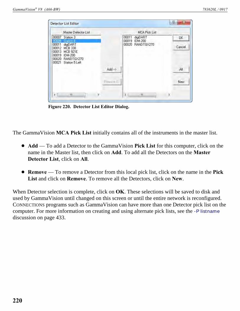
GammaVision® V8 (A66-BW) 783620L / 0917
Figure 220. Detector List Editor Dialog.
The GammaVision MCA Pick List initially contains all of the instruments in the master list.
! Add — To add a Detector to the GammaVision Pick List for this computer, click on thename in the Master list, then click on Add. To add all the Detectors on the MasterDetector List, click on All.
! Remove — To remove a Detector from this local pick list, click on the name in the PickList and click on Remove. To remove all the Detectors, click on New.
When Detector selection is complete, click on OK. These selections will be saved to disk andused by GammaVision until changed on this screen or until the entire network is reconfigured.CONNECTIONS programs such as GammaVision can have more than one Detector pick list on thecomputer. For more information on creating and using alternate pick lists, see the -P listname
discussion on page 433.
220

783620L / 0917 5. MENU COMMANDS
Figure 221. ROI Menu.
5.8. ROI
An ROI — region of interest — is a way to denote channels or groups of channels in the spec-trum as having special meaning. An ROI can be used to mark peak areas for the printout or tomark a peak to stop acquisition when that peak reaches a preset value. Channels marked as ROIchannels are displayed in a different color than the unmarked channels.
The ROI menu is shown in Fig. 221. Its functions are availablein both buffer and Detector windows. See Section 4.4.3 forROI operations performed with the mouse.
5.8.1. Off
This sets the ROI status to Off. In this state, the ROI bit for thechannels does not change as the cursor moves. This function isduplicated by <Alt + O> and by <F2> (which toggles betweenOff, Mark, and UnMark).
The usual ROI status is Off so the marker can be moved on thedisplay without changing any of the ROI bits.
5.8.2. Mark
This sets the ROI status to the Mark (set) condition. In this state, the cursor channels are markedas the cursor is moved with <6> or <7> into the channel. Moving the marker with the mousedoes not change the ROI in this mode. This function is duplicated <Alt + M> and by <F2>(which toggles between Off, Mark, and UnMark).
ROIs can also be marked with the rubber rectangle and right-mouse-button menu (seeSections 4.4.3 and 5.11.8), and as described in Section 5.8.4.
5.8.3. UnMark
This sets the ROI status to the Unmark (reset) condition. In this state, the channels are unmarkedas the cursor is moved with <6> or <7> into the channel. Moving the marker with the mousedoes not alter the ROI in this mode. This function is duplicated by <Alt + U> and by <F2>(which toggles between Off, Mark, and UnMark).
221

GammaVision® V8 (A66-BW) 783620L / 0917
5.8.4. Mark Peak
This function marks an ROI in the spectrum, at the marker position, in one of two ways.
! If the spectrum is calibrated, the region is centered on the marker with a width of threetimes the calibrated FWHM. There does not need to be a peak at the marker position.
! If the spectrum is not calibrated, the region is centered on the peak located within twochannels of the marker and as wide as the peak. If the peak search fails, or if the peak isnot well-formed, no ROI is marked. There is no limit on the size of a peak or ROI;therefore, in some uncalibrated spectra, large ROIs might be marked.
ROIs can also be marked this way with the ROI Ins button on the Status Sidebar, the MarkROI button on the toolbar, Keypad<Ins>, and <Insert>. See also Mark ROI on the right-mouse-button menu, Section 5.11.8.
5.8.5. Clear
This clears the ROI bits of all ROI channels contiguous to the channel containing the marker.This is duplicated by the ROI Del button on the Status Sidebar, Keypad<Del>, the <Delete>key, and the Clear ROI toolbar button. See also Clear ROI on the right-mouse-button menu.,Section 5.11.9.
5.8.6. Clear All
This resets all the ROI bits in the displayed spectrum (i.e., removes all ROI markings from thespectrum). However, it does not affect the ROI status of Mark/Unmark/Off.
5.8.7. Auto Clear
When this option is active (click to display a checkmark beside it) and you perform a peaksearch (see Section 5.5.2), all existing ROIs are cleared from the spectrum before the search isperformed.
5.8.8. Save File...
This allows you to save to disk a table of the channel numbers, for the current spectrum, thathave the ROI set. The contents of the spectrum are not changed.
Selecting Save File... opens a standard file-open dialog. Enter the File name. The default fileextension is .ROI. If the file already exists, the system ask if you want to overwrite the data inthe existing file or cancel the save. Click on OK to overwrite the file. \
222

783620L / 0917 5. MENU COMMANDS
Figure 222. Display Menu.
5.8.9. Recall File...
Recall File... sets the ROIs in the buffer or active Detector to the table in the disk file created byROI/Save File... (Section 5.8.8), or from the table stored in an .SPC file. This command opens astandard file-open dialog. Enter the File name. The ROIs in the buffer or active Detector will beset according to the table of values in the file. The previous ROIs will be cleared. The data con-tents of the buffer or Detector are not altered by this operation, only the ROI bits in the buffer orDetector are set.
Note that in .ROI and spectrum files the ROIs are saved by channel number. Therefore, if thespectrum peaks have shifted in position, the ROIs in the file will not correspond exactly to thespectrum data.
5.9. Display
Two of the most important functions of GammaVision areto display the spectrum data and to provide an easy andstraightforward way to manipulate the data. This is accom-plished using the Display menu functions, shown in Fig. 222,and their associated accelerators. The Display functions areavailable in both the Detector and buffer modes.
5.9.1. Detector...
Selecting this function opens the Pick Detector list shown inFig. 223. Click on a Detector on this list to display its memoryin the Full and Expanded Spectrum Views. The Pick Detectorlist shows the available Detectors, listed by Detector number,and a brief description. To close the dialog, press <Esc>.
This is duplicated by the Detector droplist on the toolbar (seepage 49). In addition, the first 12 Detectors on the list can be selected by pressing <Ctrl + F1>for the first Detector in the pick list, <Ctrl + F2> for the second Detector, and so on,through <Ctrl + F12> (see Section 9.4.8).
The current pick list is selected from the Master Detector List using Services/Edit DetectorList..., as discussed in Section 5.7.5.
223

GammaVision® V8 (A66-BW) 783620L / 0917
Figure 223. Detector Selection List.
5.9.2. Detector/Buffer
This command switches the active windowspectrum and Status Sidebar displays betweenthe last active Detector and the last active buf-fer. The Full and Expanded Spectrum Viewsdisplay the data in histogram form. This com-mand is duplicated by the accelerators <F4>and <Alt + 6>. You can also use the toolbar’sDetector droplist.
5.9.3. Select Spectrum
This menu displays a floating dialog box thatmimics the behavior of the Spectrum navigationcontrols on the sidebar when the active buffercontains an N42 file. (Section 4.5) Unlike thesidebar controls, the floating dialog can be controlled using keyboard commands.
5.9.4. Logarithmic
Logarithmic toggles the vertical scale of the Spectrum display between the logarithmicand linear modes. This function is duplicated by Keypad</> and the Log/Linear Displaybutton on the toolbar.
5.9.5. Automatic
Automatic switches the Expanded Spectrum View to a linear scale that is automatically adjusteduntil the largest peak shown is at its maximum height without overflowing the display. It alsotoggles the vertical scale of the spectrum display between the automatic and manual modes. Ifthe logarithmic scale was enabled, the display is switched to linear. This function is duplicatedby Keypad<*> and the Vertical Auto Scale toolbar button.
5.9.6. Baseline Zoom
When you select Baseline Zoom, the baseline of the spectrum displayed in the expanded view isalways zero counts. In this mode, a checkmark is displayed beside the item name on the menu.When Baseline Zoom is off (no checkmark beside the item name), the baseline can be offset to ahigher value. This is useful to show small peaks on a high background. When the baseline isoffset, the box in the Full Spectrum View is raised above the baseline to show the offset. This isduplicated on the toolbar.
224

783620L / 0917 5. MENU COMMANDS
Figure 224. Vertical and HorizontalFull-Scale Setting on the Toolbar.
Figure 225. Isotope Markers.
5.9.7. Zoom In
Zoom In adjusts the horizontal and vertical scalesin the Expanded Spectrum View to view a smallerportion of the spectrum. The vertical scale is dividedby two and the horizontal scale is reduced by about6% of the full horizontal scale. The current horizontaland vertical full-scale values are shown on the toolbar (see Fig. 224). This command is dupli-cated by Keypad<+>, the toolbar’s Zoom In button, and Zoom In on the right-mouse-buttonmenu.
5.9.8. Zoom Out
Zoom Out adjusts the horizontal and vertical scales in the Expanded Spectrum View to view alarger portion of the spectrum. The vertical scale is doubled and the horizontal scale is increasedby about 6% of the full horizontal scale. This command is duplicated by Keypad<!>, the tool-bar’s Zoom Out button, and Zoom Out on the right-mouse-button menu.
5.9.9. Center
This function forces the marker to the center of the screen by shifting the spectrum withoutmoving the marker from its current channel. This function is only required when moving themarker with the mouse; the keyboard functions for moving the marker automatically shift thespectrum to center the marker when the marker travels past the end of the current expandeddisplay. Center is duplicated by Keypad<5> and the Center button on the toolbar.
5.9.10. Full View
This function sets the Expanded Spectrum View to themaximum number of channels in the spectrum (theADC conversion gain).
5.9.11. Isotope Markers
The isotope markers can be used in energy cali-brated spectra to locate other gamma rays of thesame nuclide (from the library) when any one ofthe gamma rays from that nuclide is selected. Inthis way, you can easily see if the selected nuclideis present by comparing the spectrum peaks withthe displayed markers. The marker is a solid colorrectangle placed at the energy of the gamma ray,with the nuclide name shown above the top of the
225

GammaVision® V8 (A66-BW) 783620L / 0917
Figure 226. Isotope Markers, Expanded View.
rectangle (Fig. 225). The markers are shown in both the full and expanded views (Fig. 226). Thebase of the rectangle is positioned at the level of the background for the peak.
The amplitude of the marker for the selected peak is normally proportional to the peak area.However, the amplitude can be changed by placing the mouse in the rectangle, where it willbecome a double-sided arrow. While the double arrow is displayed, click and hold the left mousebutton and move the pointer higher or lower on the y-axis to make the rectangle larger or smal-ler. The amplitude of the marker for the other peaks is proportional to the amplitude of the firstpeak and the yield (branching ratio). As the amplitude of the peak is changed with the mouse, allthe other rectangles will change proportionally.
The markers are shown in one of two colors. If the peak area, calculated in the same manner asfor Peak Info, is positive (indicating the peak was found), then the rectangle is one color (nor-mally green). If the peak area is negative or zero (indicating the peak was not found), then therectangle is another color (normally blue).
226

783620L / 0917 5. MENU COMMANDS
Figure 227. DisplayPreferences Submenu.
Figure 228. Comparisonof the Points, Fill ROI,and Fill All DisplayModes.
5.9.12. Preferences...
This displays the options available for selecting the screencolors and spectrum display options. The submenu is shownin Fig. 227.
5.9.12.1. Points/Fill ROI/Fill All
Use these functions to select the histogram display mode forboth spectrum windows.
In Points mode, the data are displayed as points or pixels onthe screen, in the colors chosen for Foreground and ROI under Display/Preferences/SpectrumColors... (see Section 5.9.12.2).
In Fill ROI mode, the unmarked regions of the spectrum aredisplayed as points, while the ROIs are filled from the baselineto the data point with the ROI spectrum color.
In Fill All mode, all the data points are filled from the baselineto the data point with the Foreground and ROI spectrum colors.
Figure 228 shows a comparison of the three display modes. Notethat the point/pixel size in the Point- and Fill ROI-mode illustra-tions has been exaggerated to make them easier to see.
5.9.12.2. Spectrum Colors...
Use this dialog (see Fig. 229) to select colors for various featuresin the two spectrum windows. Each scroll bar controls the colorof a different feature. The vertical colored stripes behind the scrollbars show the available colors.
The Background scroll bar controls the background color of thespectrum window, Foreground determines the color of the spectrum points or fill, ROI governsthe color of the ROI points or fill. The points/fill of a compared spectrum (File/Compare...) usethe Compare color, unless they overlap with the original spectrum, in which case theComposite color is used.
Click each list and select the desired color. Changes take effect immediately. To resetto the default colors, click on Defaults. To accept the color changes, click OK. To exit withoutsaving your changes, click Cancel.
227

GammaVision® V8 (A66-BW) 783620L / 0917
Figure 229. Display Color Selections.
Figure 231. WindowMenu.
NOTE These color settings affect only the GammaVision spectrum windows.
5.9.12.3. Peak Info Font/Color
This function opens the Font dialog (Fig. 230). It allows you to select the font type, size, andcolor used to display Peak Info data in the text box in the spectrum windows (see Section 5.4.3,Fig. 130).
5.10. Window
This menu contains standard Windows commands for controllingthe display of the spectrum windows (Fig. 231). In addition to thespectrum window display mode (Cascade, Tile Horizontal, TileVertical, etc.), the list of open buffer and Detector windows isshown. The currently active spectrum is checkmarked.
The Multiple Windows command lets you choose between thenewer multiple-detector-window mode and the original single-detector-window mode. In single-window mode (no checkmarkbeside Multiple Windows), to bring another window forward asthe active window, click on its entry in the list. This is especiallyuseful if one window has been resized and has obscured otherwindows.
Figure 230. Peak Info Font/Color Dialog.
228
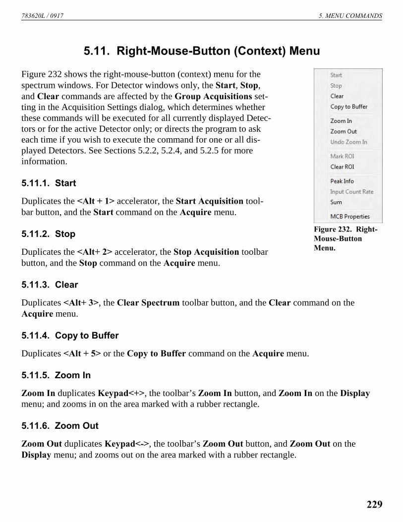
783620L / 0917 5. MENU COMMANDS
Figure 232. Right-Mouse-ButtonMenu.
5.11. Right-Mouse-Button (Context) Menu
Figure 232 shows the right-mouse-button (context) menu for thespectrum windows. For Detector windows only, the Start, Stop,and Clear commands are affected by the Group Acquisitions set-ting in the Acquisition Settings dialog, which determines whetherthese commands will be executed for all currently displayed Detec-tors or for the active Detector only; or directs the program to askeach time if you wish to execute the command for one or all dis-played Detectors. See Sections 5.2.2, 5.2.4, and 5.2.5 for moreinformation.
5.11.1. Start
Duplicates the <Alt + 1> accelerator, the Start Acquisition tool-bar button, and the Start command on the Acquire menu.
5.11.2. Stop
Duplicates the <Alt+ 2> accelerator, the Stop Acquisition toolbarbutton, and the Stop command on the Acquire menu.
5.11.3. Clear
Duplicates <Alt+ 3>, the Clear Spectrum toolbar button, and the Clear command on theAcquire menu.
5.11.4. Copy to Buffer
Duplicates <Alt + 5> or the Copy to Buffer command on the Acquire menu.
5.11.5. Zoom In
Zoom In duplicates Keypad<+>, the toolbar’s Zoom In button, and Zoom In on the Displaymenu; and zooms in on the area marked with a rubber rectangle.
5.11.6. Zoom Out
Zoom Out duplicates Keypad<->, the toolbar’s Zoom Out button, and Zoom Out on theDisplay menu; and zooms out on the area marked with a rubber rectangle.
229
GammaVision® V8 (A66-BW) 783620L / 0917
5.11.7. Undo Zoom In
This will undo or reverse the last Zoom In operation done with the rubber rectangle. It restoresthe display to the horizontal and vertical expansion before the Zoom In. It is not the same asZoom Out.
5.11.8. Mark ROI
See Sections 4.4.3 and 5.8.4.
5.11.9. Clear ROI
See Section 5.8.5.
5.11.10. Peak Info
See Section 5.4.3.
5.11.11. Input Count Rate
See Section 5.4.4.
5.11.12. Sum
See Section 5.4.5.
5.11.13. MCB Properties...
See Section 5.2.11.
230

6. ANALYSIS METHODS
6.1. General
The GammaVision program analyzes spectrum files and produces a list of the background, netarea, counting uncertainty, FWHM, and net count rate for all peaks in the spectrum. If possible,it also gives a list of the average activity of the nuclides in the sample, the activity of eachnuclide based on each gamma-ray energy in the library, the MDA for each peak energy of allnuclides in the library, and the reasons the unacceptable peaks were not used for the activitycalculation. Peaks that are not the correct shape (according to the calibration) are marked assuch; peak areas that are the result of deconvolution of overlapping energies are also marked;gamma-ray energies not in the analysis library are reported as suspected nuclides if a suitablecandidate is found in the suspected nuclide library.
The result is a report containing all the descriptions stored with the spectrum file, the analysisparameters, user inputs, and the list of peaks and nuclides found in the spectrum. The standardGammaVision report is discussed in Chapter 7.
6.2. The Analysis Engines
6.2.1. Analysis Engine Options
GammaVision includes six analysis engines, which are discussed in general terms below. Thetraditional HPGe engines were WAN32 and GAM32. NPP32 and ENV32 were created in morerecent years to address applications for which WAN32 and GAM32 were not optimized. ROI32allows you to choose which spectral regions are to be analyzed, after which the unmarked partsof the spectrum are evaluated with a simplified WAN32 analysis. The NAI32 engine is designedspecifically for low resolution spectrum analysis (i.e., sodium iodide). All six engines produce areport file (.RPT) and a binary output (.UFO) file. The following is a basic summary of processesused by each analysis engine. Section 6.2.2 contains a decision matrix to assist you in choosingan analysis routine.
6.2.1.1. WAN32
WAN32 does a preliminary library-based peak search of the spectrum. The analysis assumes thatall gamma-ray listed in the library exist in the spectrum so it tries to fit a peak at every energylisted in the library. The Peak Cutoff value specified in the Sample Defaults File (SDF) is com-pared to the 1 sigma counting uncertainty for each peak to determine if that energy will be usedfor further analysis. With a large Peak Cutoff value (> 200), this engine can “find” false peaks.A Mariscotti peak search is then implemented on the remainder of the spectrum. For nuclideswith no clean (well resolved) gamma rays WAN32 offers Manual-Based peak stripping.
231

GammaVision® V8 (A66-BW) 783620L / 0917
6.2.1.2. GAM32
GAM32 does a preliminary Mariscotti peak search of the spectrum and removes library nuclidesfor which sufficient energy peaks were not found based on Fraction limit. A library-based peaksearch is then performed using the reduced library. This analysis engine is used for specializedapplications and generally should not be selected. GAM32 overcomes the false-positive weak-ness of “library-directed” analysis when the sample is completely unknown, and the activity-accuracy weakness of the traditional “matrix” method.
In most cases, the MDA for a nuclide will not be reported because all nuclides without gammarays in the spectrum will have been removed from the library. In a few cases, the nuclide will beeliminated in the deconvolution step and the MDA will be reported for this case. To removethese possibilities, go to the System tab under Analyze/Settings/Sample Type... and selectSuppress Output from the MDA Type droplist.
For information on library reduction during GAM32 analysis, see Section 6.2.3.
6.2.1.3. NPP32
NPP32 does a preliminary library-based peak search like WAN32. Gain shift corrections can beapplied for an accurate determination of peak energy and associated nuclide activity. After theLibrary-based analysis is complete, a Mariscotti peak search is used to find any peaks that werenot included in the library or did not pass the library peak search criteria. A Directed Fit canalso be used to generate negative peak areas to meet environmental reporting requirements forsinglet peaks. Standard reports have a “Summary of Peaks in Range” section that displays poten-tial library matches and associated activity concentration for each peak found during analysis.NPP32 and ENV32 do especially well with Library-Based peak stripping.
For the deconvolution of multiplets in the re-analysis phase, the peaks are allowed to shift inenergy, up to two channels. The entire multiplet moves as a group. This gives more accuratepeak areas when the energy shifts between the calibration and the sample spectrum. (Note thatthis is in addition to the recalibration for energy for the entire spectrum.)
6.2.1.4. ENV32 and NAI32
ENV32 and NAI32 are very similar in operation, but designed for different spectrum types -ENV32 for HPGe, and NAI32 for Sodium Iodide and other lower resolution detector types.These engines optionally perform a preliminary Mariscotti peak search of the spectrum andremove library nuclides for which sufficient energy peaks were not found. A library-based peaksearch is then performed using the reduced library. Gain shift corrections can be applied for anaccurate determination of peak energy and associated nuclide activity. Directed Fit can also beused to generate negative peak areas to meet environmental reporting requirements for singlet
232

783620L / 0917 6. ANALYSIS METHODS
(22)
and multiplet peaks. Standard reports have a “Summary of Peaks in Range” section that displayspotential library matches and associated activity concentration for each peak found duringanalysis.
See Section 6.2.3 for more information on the library reduction process.
6.2.1.5. ROI32
The ROI32 analysis engine operates on the entire spectrum, performing an ROI analysis on user-marked ROIs and a modified WAN32 analysis (no peak stripping or directed fit) on unmarkedregions. You can either mark ROIs on a live or retrieved spectrum, then use the Analyze/EntireSpectrum in Memory command; or use the Analyze/Spectrum on Disk command on aspectrum file in which ROIs have already been marked and saved.
ROI Analysis
1) The ROI center is used to calculate the ROI peak energy using the existing energy calibra-
tion. If the ROI peak energy is within the match width of a library peak, then the ROI will beused. Otherwise, the ROI will be ignored. In other words, do not mark an ROI aroundunknown peaks.
2) To calculate the ROI peak background, you can set the number of background points to beused at 1, 3 or 5 on the Sample tab under Analyze/Settings/Sample Type.... If Auto back-ground is selected, then 5 points will be used always. The background points to be used forthe background calculation are within the selected ROI region, not adjacent and outside theROI region.
3) The background of the ROI peak is calculated as:
where:L = the lowest-energy channel of the ROIH = the highest-energy channel of the ROIN = 1, 3, or 5, depending on the background method chosen, as discussed above.
and the sum of background counts on the low and high end of the ROI, B1 and B2,respectively, are given by:
233

GammaVision® V8 (A66-BW) 783620L / 0917
(25)
(26)
(27)
(23)
(24)
whereCLB = counts per background channel at the low end of the ROICHB = counts per background channel at the high end of the ROI
4) The gross counts within the ROI are calculated as:
5) The net peak area is the adjusted gross counts minus the adjusted calculated background, asfollows:
thus:
where all parameters have been defined above. If the 3-point background method is chosenon the Sample tab (page 150), all three parameters calculated above — B, G, and A — shouldbe the same as calculated with the Peak Info method (Section 5.4.3).
6) This simplifies to:
Additional Considerations
! If there are multiple ROIs defined for a nuclide, then only the first ROI peak is used to
calculate the nuclide activity.
234

783620L / 0917 6. ANALYSIS METHODS
! In ROI32 engine, if a nuclide has multiple peaks and only one peak is marked with a ROI,then the nuclide activity displayed is the activity of only the marked ROI peak.
! In the WAN32 analysis results section of the report, the nuclide activity is the same as theactivity reported in the ROI Peak Summary section of the report.
6.2.2. Selecting an Analysis Engine — Decision Matrix
A library-based peak search looks for potential peaks for all gamma rays listed in the library.
Sensitivity is set by the Peak-Cutoff settings. A Mariscotti peak search uses a second differen-tial method to identify peaks. Sensitivity is set by the Peak-Search Sensitivity setting. Mari-scotti peak searches do a better job of identifying peaks within multiplets; library-based peaksearches will do a better job of finding a weak or misshapen peak listed in the library.
Feature ENV32
WAN32 NPP32 GAM32 ROI32 NAI32
Uses an optional initial Mariscotti peak search % % %
Uses an initial library-based peak search % % %
ROI peak search on user-marked peaks %
Library based peak stripping % % % %
Manual based peak stripping %
Removes nuclides from library not found in apreliminary peak search
% % % %
Reports MDA for removed nuclides % % %
Utilizes gain shift corrections % % % % %
Directed fit (negative or misshapen peakareas) option available
%a %b %b %a
More sensitive in finding misshapen peaks % % %
Displays all possible library nuclide matchesand calculates activity for all peaks found.
% % % %
Peak Search designed for High Resolution (H)(i.e., HPGe) or Low Resolution (L) (i.e.,Sodium Iodide) spectra
H H H H H L
aSinglets and multiplets.bSinglets only.
235

GammaVision® V8 (A66-BW) 783620L / 0917
6.2.2.1. Guidelines for Selecting an Analysis Engine
1) Decide which peak search method is best for your application.
2) Establish the sensitivity for the peak search (Peak Cutoff for library directed; Sensitivity forMariscotti).
3) Decide if an accurate analysis of the multiplets is important. If so, select NPP32 or theENV32 analysis engine.
4) Notice if there are false negatives in your answers. That is nuclides have been initiallydetected and later dropped. If so, revert to the WAN32 analysis engine.
6.2.3. Library Reduction Based on Nuclide Rejection (ENV32, GAM32 and NAI32Analysis Engines Only)
The Library Reduction step is optionally enabled or disabled with the “Library Reduction Flag”in the b30winds.ini (or n30winds.ini for NAI32) file (Section A.2.2.1). By default, this setting isenabled for HPGe analysis (b30winds.ini) and disabled for Sodium Iodide analysis(n30winds.ini). If enabled, a raw peak search is performed on the spectrum. The list of peaksfound is compared to the peaks in the library, and the nuclides not likely to be present areremoved from the library. After the library is reduced, a search is performed for the remaininglibrary peaks, and the raw data (Mariscotti) peak search is run again to pick up any peaks notaccounted for in the library-directed search. If Directed Fit is turned on, then peaks fromnuclides that were previously rejected are fit using the Directed Fit method (Section 6.3.2.2) andthe activity is calculated.
6.2.3.1. Library Reduction based on Peak Order
The following process is used for the library reduction when the “ENV factor” in theb30winds.ini (n30winds.ini for NAI32) (Section A.2.2.1) is not set to zero:
1) If the first peak for a nuclide in the library is not found meeting the peak cutoff, then thatnuclide is removed from the analysis.
2) If the first peak for a nuclide in the library is found meeting the peak cutoff limit then eachsubsequent peak for that nuclide (to a maximum of three peaks per nuclide) is evaluated todetermine if the nuclide should be removed from the analysis as follows:
3) For each subsequent peak i (to the maximum of three per nuclide), evaluate as follows:
If then
236

783620L / 0917 6. ANALYSIS METHODS
Go to the next peak,
Else,
a) Calculate the expected peak area for the ith peak as:
b) Calculate the critical level Lc for the ith peak as:
If Ai > Lc and the ith peak is not a valid peak (that is, the peak is not found or the peakuncertainty is greater than the peak cutoff), then the nuclide is removed from the library.
Next peak i.
where:E1 = efficiency for the first valid peakBr1 = branching ratio for the first valid peakEi = efficiency for subsequent library peaksBri = branching ratio for subsequent library peaksA1 = activity calculated for the first nuclide peakAi = activity calculated for subsequent library peaksBi = peak background for subsequent library peaksW = peak width for subsequent library peaksM = number of total points outside the peak used to calculate backgroundENV = user-adjustable ENV factor from the b30winds.ini (n30winds.ini for NAI32)
file located in C:\Program Files\GammaVision (Section A.2.2.1). A setting ofzero disables this reduction process, but the reduction based on the Key Lineand Fraction Limit test in the next step still occurs.
6.2.3.2. Library Reduction Based on Key Line and Fraction Limit Tests
In this library reduction algorithm, the key line and fraction limit tests are carried out todetermine if nuclides will be removed.
For the key line test, the first in-range peak for a nuclide is always considered as a key line, evenif it is not marked as a key line. All key lines for a nuclide must be found in the spectrum, even ifthe key line has overlap with another library peak. If any of the qualifying key lines are not
237
GammaVision® V8 (A66-BW) 783620L / 0917
found, the key line test fails and the nuclide is rejected.
If the fraction limit is not zero then the fraction of the branching ratios is calculated by summingthe branching ratios of all identified peaks and dividing by the sum of all peak branching ratioswhether identified or not. If the calculated fraction is less than the Fraction Limit set on theAnalysis tab, the nuclide is rejected.
If the “Fraction Limit Test flag” in b30winds.ini (n30winds.ini for NAI32) is False andDirected Fit is enabled on the System tab, the library peak flags are checked to determine if apeak is “qualified” for its branching ratio to be summed (in the total sum and the identified peaksum). Peaks with the “Not In Average” flag set in the library are excluded along with peaksoutside the analysis range.
6.3. Calculation Details for Peaks
For all library peaks in the analysis energy range, the program attempts to calculate the net peakarea and centroid of a peak at that channel. At this step in the analysis, each peak is consideredto be a singlet. A singlet is a single, isolated peak; that is, it is far enough away from other peaksin the spectrum so that the spectrum is background on both sides of the peak (does not overlapanother peak).
6.3.1. Background Calculation Methods
You can select the method from among these types: automatic, X-point average, and X * FWHM(see Section 5.5.1.1).
6.3.1.1. Automatic
For the first pass, the peak centroid is the library energy (Fig. 233).
To calculate the first pass background on the low-energy side of the peak, the 5-point average ofthe channel contents is calculated for the region from the peak-centroid channel to the channelwhich is 6 times the library match width (normally 0.5) times the calculated FWHM (from thecalibration) below the centroid. The 5-point average data at a given point is the sum of the datafrom two channels below the point to two channels above the point divided by 5. This is thesame as smoothing the data with a smoothing width of 5 and coefficients of 0.2 for all points.The background value is the minimum value of the moving 5-point average and the backgroundchannel number is the center channel of the 5. If the minimum average value is within one sigma(counting statistics) of the actual channel value at the assigned channel point, this 5-point
238

783620L / 0917 6. ANALYSIS METHODS
Figure 233. Background Calculation.
average is the low energy background value for this peak. If the average value is not within one sigma of the actual data, a 3-point average is used instead of the 5-point average to calculate anew minimum value. This 3-point average minimum value is compared with the actual data atthe assigned channel and is accepted if it is within 1 sigma of the actual data. If the 3-pointaverage also fails this test, the data value at the assigned channel is used for the background.
The same process is repeated for the high-energy side of the peak to calculate the backgroundvalue above the peak. The background under the peak is the straight line between these twovalues.
The net peak area and background are calculated from this first pass. Next, the width is reducedor increased depending on the peak-area-to-background ratio and the library match width. Thisadjustment makes two improvements: (1) it reduces the number of channels in the peak for smallpeaks (decreasing the uncertainty), and (2) it improves the area calculation for peaks movedfrom the library energy.
This background calculation method (that is, automatically selecting 5-, 3-, or 1-point averaging,depending on which method best approximates the spectrum data) has advantages, when thereare closely spaced peaks, over other methods. For example, because the 1-point method will beused when a small peak is very near a large peak, a more accurate measure of the backgroundmay be obtained as compared to using more points in the average (Fig. 234).
239
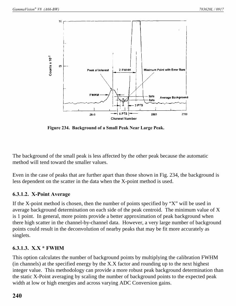
GammaVision® V8 (A66-BW) 783620L / 0917
Figure 234. Background of a Small Peak Near Large Peak.
The background of the small peak is less affected by the other peak because the automaticmethod will tend toward the smaller values.
Even in the case of peaks that are further apart than those shown in Fig. 234, the background isless dependent on the scatter in the data when the X-point method is used.
6.3.1.2. X-Point Average
If the X-point method is chosen, then the number of points specified by “X” will be used inaverage background determination on each side of the peak centroid. The minimum value of Xis 1 point. In general, more points provide a better approximation of peak background whenthere high scatter in the channel-by-channel data. However, a very large number of backgroundpoints could result in the deconvolution of nearby peaks that may be fit more accurately assinglets.
6.3.1.3. X.X * FWHM
This option calculates the number of background points by multiplying the calibration FWHM(in channels) at the specified energy by the X.X factor and rounding up to the next highestinteger value. This methodology can provide a more robust peak background determination thanthe static X-Point averaging by scaling the number of background points to the expected peakwidth at low or high energies and across varying ADC Conversion gains.
240

783620L / 0917 6. ANALYSIS METHODS
Figure 235. Example Peak Background Calculation.
6.3.1.4. Example Background
An example is shown in Fig. 235, with the spectrum printout in Table 5. The report section forthis peak is shown in Fig. 236.
The FWHM for this peak is 6.85 channels. The centroid is at channel 2292.16. The backgroundsearch width is from channel 2271 to 2313. The 5-point averages are shown in Table 5, and theminima are 11.8 at channel 2276 and 12.2 at channel 2311. The background slope is +0.0114and the offset is !14.4.
241

GammaVision® V8 (A66-BW) 783620L / 0917
UNIDENTIFIED PEAK SUMMARY
PEAK CENTROID BACKGROUND NET AREA INTENSITY UNCERT FWHM SUSPECTEDCHANNEL ENERGY COUNTS COUNTS CTS/SEC 1 SIGMA % keV NUCLIDE
2292.16 569.78 432. 17711. 59.04 .81 1.734 Bi-207
s Peak fails shape tests.
Figure 236. Peak Results for Previous Peak.
Table 5. Spectrum and Five-Point Smooth.
Fig. 237 shows an example of the differences among the four methods for determining the
242

783620L / 0917 6. ANALYSIS METHODS
PEAK CENTROID BACKGROUND NET AREA INTENSITY UNCERT FWHM CHANNEL ENERGY COUNTS COUNTS CTS/SEC 1 SIGMA % keV+-+-+-+-+-+-+-+-+-+-+-+-+-+-+-+-+-+-+-+-+-+-+-+-+-+-+-+-+-+-+-+-+-+-+-+-+-+-+-+-+ Background width: best method (based on spectrum). 2939.64 718.00 1514. 79. .009 70.82 1.517
Background width: average of five points. 2939.64 718.00 1372. 12. .001 422.37 1.517
Background width: average of three points. 2939.64 718.00 1299. 43. .005 119.77 1.517
Background width: minimum data point. 2939.64 718.00 1214. 72. .008 69.70 1.517
Figure 237. Example of Different Background Method Results.
(30)
background.
6.3.2. Peak Area — Singlets
6.3.2.1. Total Summation Method
The gross area of the peak is the sum of the contents of each channel between the backgroundchannels (including the two background channels) as follows:
where:Ag = the gross areaCi = the data value of channel il = the center channel of the background calculation width at the low energy side of the
spectrumh = the center channel of the background calculation width at the high energy side of the
spectrum
This peak area calculation method (referred to as total summation) maintains precision as thepeak gets smaller, is less sensitive to random fluctuations in the data, and is less sensitive to thedifferences between the spectrum peak shape and the calibrated peak shape.
Refer to Fig. 235, Fig. 236, and Table 5 to calculate the gross area for the example peak. Theintegral from channel 2276 to 2311 is 18143 counts.
The net area is the gross area minus the background in those channels (Fig. 238).
243

GammaVision® V8 (A66-BW) 783620L / 0917
Figure 238. Gross and Net Peak Area.
(31)
where:Ab = the background areaBl = the background on low side of peakBh = the background on high side of peakW = the peak width
If the PBC correction is enabled, the calculation is performed as discussed in Section 6.10.4.
6.3.2.2. Directed Fit Method
In some cases the total summation method does not produce the desired answer for the peak areaand does not produce negative peak areas. Another method of obtaining the peak area for aparticular energy is to fit the spectrum region with a background plus peak shape function. Thisso-called “directed fit” — enabled on the Analysis tab — can be applied to peaks and has theability to produce negative peak areas, and therefore, activity results less than zero.
The directed fit to the library peak area is performed if the following are true:
1) The option is enabled.2) The spectrum is energy calibrated.
244

783620L / 0917 6. ANALYSIS METHODS
(32)
(33)
3) The peak was rejected for any test by the total summation method.
Directed Peak Fit for singlet peaks is determined using a range of 4.84 times the calibrationFWHM times the Analysis Settings Match Width times the Directed Fit Peak Region WidthFactor (Section A.2.2.1) centered on the library peak energy. For multiplets, the range is basedon the start channel of the first peak minus the background width and the stop channel of the lastpeak plus the background width.
Background, Gross Area, and Net Area are then calculated as described in Section 5.4.3. Thenet area is then corrected for contributions from identified nuclide peaks and peak backgroundby adding these areas to the background. Any remaining area is assigned to the Directed Fitnuclide peak. When multiple nuclides have interferences at approximately the same energy thefirst nuclide that is dependent on that peak energy for the activity calculation is evaluated first,and nuclides that have peaks that are not interfered are evaluated afterwards.
6.3.2.3. ISO NORM Singlet Peak Method
The guidelines for singlet peak calculations are in Annex C of the ISO 11929:2010 standard, andare similar to the standard GammaVision total summation method discussed in Section 6.3.2.1.
When the peak background does not dominate, the peak width should be ~2.5 FWHM, per ISO11929 Eq. C.9:
where h is the FWHM of the peak.
In case of a dominant background, the peak region width should be 1.2 FWHM, per Eq. C.10:
When tg is 2.5, almost the entire peak area is included in the region. However, when tg is 1.2, thepeak region only covers about 84% of the whole peak area. Therefore, a correction factor for thepeak area is needed, as discussed in the remainder of this section.
In GammaVision, the percent Peak Cutoff, entered on the Analysis tab, is used by default as thecriterion for dominant background. Background is considered dominant except when the peakuncertainty is less than the Peak Cutoff, in which case the peak is flagged as “identified.”Therefore, for all identified singlet peaks, the default region width should be about tg × FWHMfor this method.
245

GammaVision® V8 (A66-BW) 783620L / 0917
(34)
(35)
(36)
(37)
(38)
If the library peaks are not found, the MDA values are calculated with a width of ~1.2 FWHM.Since the exact criteria for dominant background are not specified in ISO 11929, GammaVisionincludes a “Dominant Background Peak Cutoff and Override Flag” in the b30winds.ini
(n30winds.ini for NAI32) file (Section A.2.2.1) to enable you to define a dominant backgroundcutoff. This entry is formatted as:
25.0 T
The first parameter is the user-defined dominant background peak uncertainty cutoff. The defaultvalue is 25%, and ranges from >0% to <1000%. The second parameter is a Boolean flag. If theflag is set to false (F), the user-defined peak cutoff for dominant background is used. If the flagis true (T), the Peak Cutoff value on the Analysis tab is used.
To calculate a correction factor when the peak region does not cover all the peak area, let thepeak region width be í (in units of the peak FWHM):
Assume the peak shape is a perfect Gaussian. Let f be the ratio between the net counts in theregion and the true total peak area, then f can be calculated as:
where Ö is a Gaussian integral function defined as:
and c is a constant equal to:
The correction factor f is used as a divisor in the calculations of the peak area:
where N0 is calculated with the region width chosen per ISO 11929. The f factor is not usedwhen N0 is zero or negative since no peak is present and a negative peak area is non-physical.
246

783620L / 0917 6. ANALYSIS METHODS
(39)
(40)
(41)
(42)
(43)
(44)
The use of f is consistent with Eq. D.5 in ISO 11929:
The definition of the quantities involved in above equation can be found in section D.5.1 ofISO 11929. The factor f in the denominator is defined in Eq. 35 above, and i is the branchingratio. The f factor is not used to scale the peak background. The background does not scale asthe peak area (that is, even though 84% of the peak area is covered, it is incorrect to state thatonly 84% of the background is included).
When x is positive, the Gaussian integral Ö(x) can be calculated as:
where Erfc(x) is the Complimentary Error Function:
The Complimentary Error Function is calculated using the following analytic approximation:30
where t and ö are defined in the following equations:
30Press, W. H., et al., Numerical Recipes in C: The Art of Scientific Computing, Cambridge University Press; 2nded. (October 30, 1992).
247

GammaVision® V8 (A66-BW) 783620L / 0917
(45)
where:a0 = 1.26551223a1 = 1.00002368a2 = 0.37409196a3 = 0.09678418
a4 = !0.18628806a5 = 0.27886807a6 = !1.13520398a7 = 1.48851587a8 = !0.82215223a9 = 0.17087277
The approximation work wells for the range of x values we are concerned with.
To calculate the actual peak region start and stop channels, the half width of the region is calcu-lated first, e.g., 0.5 tg. This half width is converted by rounding to an integer, in channels, with alower limit of 1 channel. For best precision, the analysis engine compares the rounded-down androunded-up values and selects the best match to the desired overall regional width. For high-energy peaks, it may not matter whether the integral width is rounded down or up, however,there may be a big difference for some low-energy peaks. For example, if the energy calibrationat low energies is ~0.5 keV per channel and the calibrated peak FWHM is ~1.0 keV, the differ-ence between the two rounding methods could be as great as one FWHM. For a desired peakregion width of 1.2 FWHM, the width obtained by rounding up could be about 2.2 FWHM,defeating the intent to use a narrow peak width when the background is dominant.
The ISO peak evaluation method is applied only for peaks that meet the following requirements:
1) The peak is in the library.2) The peak range, including the designated number of background points, has no overlap with
both lower or higher energy peaks. 3) The energy separation between the current peak and the nearest low- and high-energy peaks
should be greater than the separation for deconvolution (the latter determined by the “Peakoverlap range in units of peak FWHM” parameter in b30winds.ini (n30winds.ini for NAI32).
4) The peak shape is close to Gaussian. Peaks marked with * or @ on the report do not qualify. 5) The peak centroid cannot be too far from the library energy. Peaks marked with } on the
report do not qualify.
248

783620L / 0917 6. ANALYSIS METHODS
(46)
(47)
Figure 239. Example of Directed Fit.
6.3.3. Example Peak Area
6.3.3.1. Total Summation Method
Again, refer to Fig. 235, Fig. 236, and Table 5 to calculate the background for this peak (PBCcorrection disabled). Substituting in the above formulas yields:
and
6.3.3.2. Directed Fit Method
A section of a spectrum with a negative peak is shown in Fig. 239. The raw data values and thegenerated fit are shown. In this case the, background at the low energy end of the peak is1170 counts per channel and on the high end is 1173 counts per channel. This gives a total back-ground of 35145 counts and the net peak of !133 counts.
Since these values are derived from a fitting process, it is difficult to duplicate the calculationsmanually.
249

GammaVision® V8 (A66-BW) 783620L / 0917
(48)
(49)
6.3.4. Peak Uncertainty
The counting statistical uncertainty is the uncertainty in the gross area and the uncertainty in thebackground added in quadrature. The uncertainty in the gross area is the square root of the area.The uncertainty in the background is not as simple because the background is a calculated num-ber. The background area uncertainty is the uncertainty in the channels used to calculate the endpoints of the background multiplied by the ratio of the number of channels in the peak to thenumber of channels used to calculate the background. For wide peaks and low counts per chan-nel, there is high uncertainty in the calculated background.
If the PBC correction is enabled, the uncertainty calculation is performed as discussed inSection 6.12.12.
PBC correction is disabled for the following example. Referring back to Fig. 235, Fig. 236, andTable 5, the background uncertainty is:
The peak width is calculated at the half maximum, tenth maximum, and twenty-fifth maximumfor the net peak shape. The peak width points are linearly interpolated between the two channelsthat bracket the respective height value.
6.3.4.1. Peak Uncertainty in ZDT Spectra
This is discussed in Section 5.2.11.4.
250

783620L / 0917 6. ANALYSIS METHODS
(50)
6.3.5. Peak Centroid
The peak centroid channel in total summation is the center-of-moment of the peak and is calcu-lated as the weighted channel number of the peak. That is, the peak centroid is the sum of the netchannel contents times the channel number divided by the sum of the channel contents. Thecentroid is calculated as:
where:l, h = the peak low and high channelsi = the channel numberCi = net contents of channel i
For the directed fit method, the centroid can be refined from the fitting process.
From the Table 5 values and the calculated background, the net spectrum is shown in Table 6,continuing the example calculation on this peak.
The FW.04M is 2.2 times the FWHM for a Gaussian peak. The peak integration channels arethen 2284 to 2300. The channel numbers are rounded to the nearest integers. The centroid forthis example is 4.0366×10⁷ / 1.761×104 = 2292.16.
6.3.6. Energy Recalibration
The spectrum energy calibration can be redone “on the fly” for the spectrum being analyzed.This improves the analysis results and adjusts for small changes in the hardware gain. Energyrecalibration is first performed using singlet peaks only. Then, after deconvolution, the spec-trum is recalibrated using all the peaks. If the energy calibration changes, the spectrum isreanalyzed.
For all peaks in the library, the peak centroid energy in the spectrum is compared with thelibrary energy. If the difference between the library energy and the centroid energy is lessthan 0.5 keV, or the current Match Width (the FWHM multiplier entered on the System tab
251

GammaVision® V8 (A66-BW) 783620L / 0917
Channel Background Net Spectrum2270 11.7152 5.2842271 11.7266 2.2732272 11.7380 2.2622273 11.7494 2.2502274 11.7608 -4.7602275 11.7722 0.2272276 11.7836 3.2162277 11.7950 4.2052278 11.8064 -2.8062279 11.8178 4.1822280 11.8292 -1.8292281 11.8406 9.1592282 11.8520 20.1482283 11.8634 15.1362284 11.8748 47.1252285 11.8862 120.1132286 11.8976 225.1022287 11.9090 461.0912288 11.9204 835.0792289 11.9318 1369.0682290 11.9432 1887.0572291 11.9546 2321.0462292 11.9660 2391.0342293 11.9774 2393.0232294 11.9888 1972.0112295 12.0002 1503.0002296 12.0116 933.9882297 12.0230 622.9772298 12.0344 295.9652299 12.0458 175.9542300 12.0572 56.9422301 12.0686 28.9312302 12.0800 11.9202303 12.0914 -2.0912304 12.1028 -1.1022305 12.1142 1.8852306 12.1256 1.8742307 12.1370 1.8632308 12.1484 4.8512309 12.1598 3.8402310 12.1712 -4.1712311 12.1826 1.8172312 12.1940 1.8062313 12.2054 -3.2052314 12.2168 9.7832315 12.2282 -4.2282316 12.2396 -1.2392317 12.2510 -2.2512318 12.2624 1.7372319 12.2738 -0.273
Table 6. Example Net Spectrum.under Analyze/Settings/Sample Type...), orone channel — whichever is greater — thatcentroid is associated with that library energy.The FWHM multiplier can be changed. If it iswithin this limit and has counting error lessthan 10% or the input sensitivity value (which-ever is less), it is a qualified recalibration peak.
The energy range is split into two parts and thenumber of qualified library peaks in each regionis counted. It there are more than the user-setnumber of qualified recalibration peaks in bothregions of the spectrum, these spectrum cen-troids and library energies are used to recalcu-late the energy calibration for the spectrum.The default energy is 0 keV and the number ofpeaks is 1000 below and 1000 above. Only thisanalysis is affected and the calibration in thespectrum file is not changed. If the energyrecalibration is performed, a notice is written onthe report, even if the recalibration had little orno effect. The new coefficients are printed onthe output report.
Since this energy recalibration is dependenton the library and the spectrum, changes in thelibrary can affect the calibration, and hencethe peak energies reported. Only the energyfactors are changed. The shape coefficient andefficiency coefficients are not altered. Whilethe automatic energy recalibration will correctfor small changes in the calibration, it is notintended as a substitute for accurate calibra-tions or as a correction for systems sufferingfrom stability problems.
For an accurately calibrated spectrum, thisrecalibration will have little effect. Its effectwill be most pronounced on deconvolutionsof multiplets; this is discussed in Section 6.5.
252

783620L / 0917 6. ANALYSIS METHODS
(51)
Because of this recalibration feature, the analysis results of spectra can change when a library ischanged, or if the peak sensitivity is changed to a value under 10% (see fixed cutoff above).Such changes between analyses can result in the recalibration being enabled in one case anddisabled in the other case. This can result in the analyses being different in several differentways. The peak areas and backgrounds can be different because the integration limits for eachpeak will change slightly. This change is usually very small, but in a spectrum with very fewcounts it can be a high percentage of the total peak. In a given spectrum, some peak areas mightchange and others might be constant. Some peaks might move from the identified list to theunknown list (or the reverse) because the uncorrected centroid is too far from the library energyfor validation.
In addition, an energy difference for all good library peaks is calculated. This is the sum of theabsolute value of the difference between the peak centroid energy (before recalibration) and thelibrary energy, expressed as a fraction of the FWHM, divided by the number of peaks in the sum.This yields a number between 0 and 1 for good 3-point (or more) calibrations, with 0 being thebest calibration. For 2-point calibrations, this number can be much larger than 1.0 because thecalculated FWHM (which is a linear function) does not fit the spectrum FWHM at the ends ofthe spectrum. If high values are reported, and the analysis results are unacceptable, a better cali-bration should be made. The calibration section can be used to produce a multi-point calibrationwhich will reduce the energy difference.
where:Epi = the energy of the ith peak in the spectrumELi = the energy of the corresponding peak in the libraryFWHMLi = the calculated FWHM of the peak at the libraryn = the number of peaks in a spectrum with matching library peaks
This “energy-normalized difference” is printed on the report. For a complex spectrum thisnumber will range from 0.1 to 0.3. A large value indicates that a new calibration should beperformed or that the library does not match the spectrum well. Smaller values are usuallyassociated with fewer peaks or a better calibration.
If an energy recalibration has occurred, the library peak list is reanalyzed with the new energycalibration. This results in more accurate peak values for centroid and area.
253

GammaVision® V8 (A66-BW) 783620L / 0917
Figure 240. Second Difference.
(52)
6.3.7. Peak Search
After the library peaks are located, the spectrum is searched for any other peaks. This is needed,even if the list of unknown peak values is not requested, for correct calculation of the peak back-ground near peak multiplets and for determination of the peak centroids for deconvolution ofmultiplets not in the library. The stepped background test compares the background above thepeak area to the background of the peak area (see “Background for Multiplets,” Section 6.5.2).
The peak search method is based on the method proposed by Mariscotti. In this method it isassumed that the spectrum, C(n), is continuous and the background is a linear function of thechannel number in the vicinity of a peak. This implies that the second derivative is zero for back-ground regions and non-zero in the peak regions. In order to reduce the effect of statistical fluc-tuations, the smoothed second difference is used (see Fig. 240).
The second difference can be represented as:
where:ki = the smoothed second difference weighting functions2j +1 = the smoothing width
254
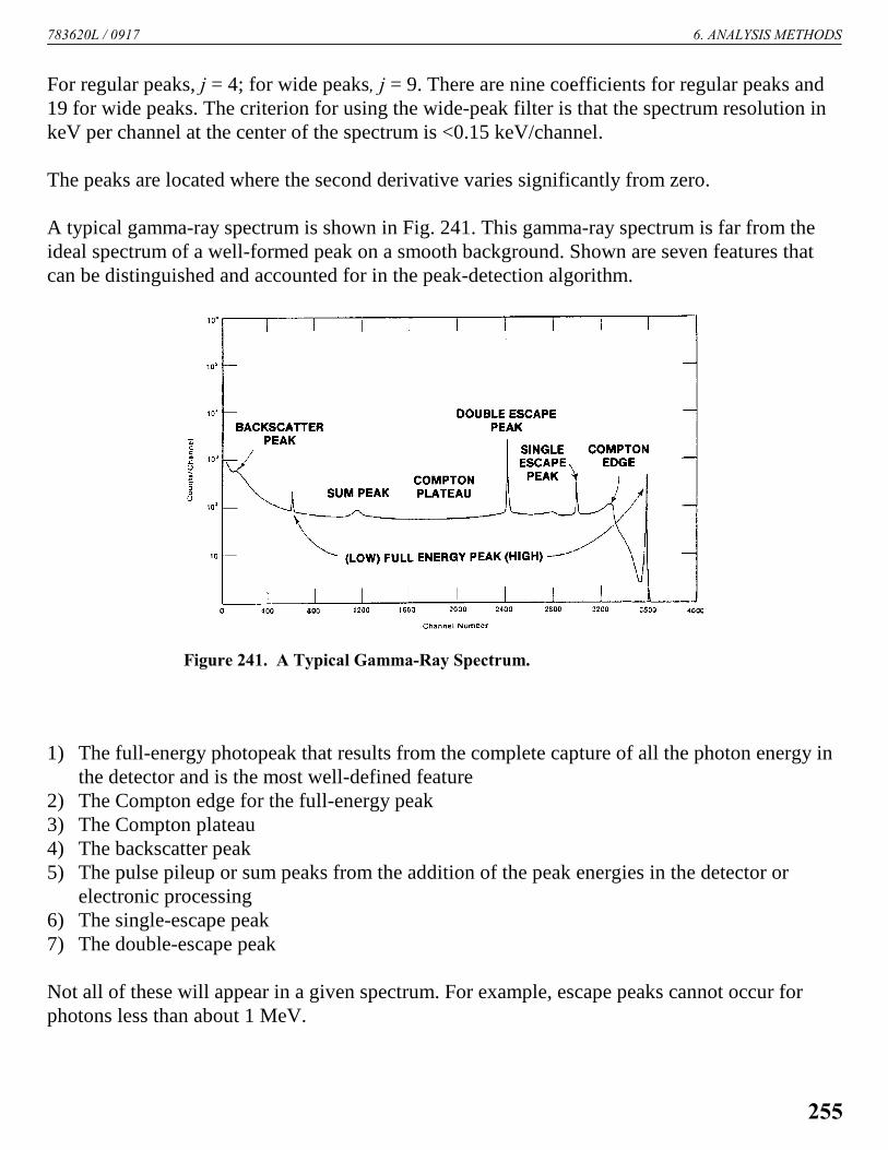
783620L / 0917 6. ANALYSIS METHODS
Figure 241. A Typical Gamma-Ray Spectrum.
For regular peaks, j = 4; for wide peaks, j = 9. There are nine coefficients for regular peaks and19 for wide peaks. The criterion for using the wide-peak filter is that the spectrum resolution inkeV per channel at the center of the spectrum is <0.15 keV/channel.
The peaks are located where the second derivative varies significantly from zero.
A typical gamma-ray spectrum is shown in Fig. 241. This gamma-ray spectrum is far from theideal spectrum of a well-formed peak on a smooth background. Shown are seven features thatcan be distinguished and accounted for in the peak-detection algorithm.
1) The full-energy photopeak that results from the complete capture of all the photon energy inthe detector and is the most well-defined feature
2) The Compton edge for the full-energy peak3) The Compton plateau4) The backscatter peak5) The pulse pileup or sum peaks from the addition of the peak energies in the detector or
electronic processing6) The single-escape peak7) The double-escape peak
Not all of these will appear in a given spectrum. For example, escape peaks cannot occur forphotons less than about 1 MeV.
255

GammaVision® V8 (A66-BW) 783620L / 0917
Figure 242. Second Difference for a Compton Edge.
(53)
(54)
The shape of the second derivative can be used to reject Compton edges and other non-peakstructure in the data (Fig. 242).
6.3.7.1. Peak Acceptance Tests
The second difference must pass the following tests to be considered a peak.
where G is related to S, the PEAK SEARCH SENSITIVITY factor, set on the System tabunder Analyze/ Settings/Sample Type..., as follows:
where:G = a constant proportional to the resolution of the detectorF = 1.35 for the wide-peak filter and 1.0 for the regular-peak filter
In addition, the spectrum data at the channel indicated by the second derivative must pass thesetests.
256

783620L / 0917 6. ANALYSIS METHODS
(55)
(56)
(57)
where:C(n) = the channel data of the nth channelCO(n) = the second difference at the nth channel
If the wide-peak filter is used, the second derivatives must also meet the following criterion:
The peak centroid is calculated using the weighted channel sum method as follows:
where:P = peak centroid in channelsCi = net contents of channel ii = channel numberl = peak low limith = peak high limit
Once a peak is located, it is recorded and the peak search starts again.
After a peak has been located, if it is not in the library, the peak background, net area, anduncertainty are calculated in the same manner as library peaks. If the peak uncertainty is lessthan the sensitivity threshold level you entered, the peak is added to the list of unknowns. If thepeak is within the deconvolution width (approximately 3.3 times the FWHM) of a library peak,then the peak is marked on the output list. The unknown peaks are included in a deconvolutionwhen they are close enough to affect the peak area calculation.
If a peak is located in the spectrum and the library peak is a subsidiary peak, where the majorpeak has not been found, the peak will be maintained in the unknown list.
257

GammaVision® V8 (A66-BW) 783620L / 0917
6.3.8. Narrow Peaks
The peak width is compared to the calibration width at the half and tenth maximum. If the peakis too wide or too narrow it is marked to show this in the output report. If the peak is too narrow,it is not used in the abundance calculation unless the “accept-low-peaks” or “accept-all-peaks”switch (T=accept low peaks, page 440) is turned on. If accept-all-peaks is on, all are accepted. Ifaccept-low-peaks is on, the peak is further tested. If the peak area is less than 200 counts, it isaccepted. If the peak area is between 200 and 300 counts and the background is less than half thepeak area, the peak is accepted. If the peak area is over 300 it is rejected.
6.4. Suspected Nuclides
The suspected nuclides feature will identify peak energies in the unknown peak list, based on asecond gamma-ray library. The unknown peak list is the list of all peaks located in the spectrumthat are not in the analysis library. It is intended to help identify unexpected peaks or can be usedto note peaks that are always present but for which no analysis is desired (e.g., 40K or 511 keV).The name for the suspected nuclide library is specified on the System tab under Analyze/Settings/Sample Type....
For each energy listed in the unknown peak list, the nuclide with the closest energy within fourtimes the FWHM is listed. In the event that two energies are found with the same difference, thelowest energy entry in the library is printed. If none is found, a symbol is printed. In addition, thesame symbol is printed if the suspected library is not found, a read error occurs, or the spectrumis not calibrated.
The suspected nuclide feature can be used with calibrated spectrum files (and no analysislibrary) to obtain a quick list of nuclides in the sample and their peak count rates.
6.5. Locating Multiplets
A peak is considered to overlap if its start or end channels are within another peak region. Thepeak overlap range factor in b30winds.ini (n30winds.ini for NAI32) determines whether twopeaks close in energy will be deconvoluted as a multiplet or stripped. The lowest setting for thisparameter is 1.0.
If the library energies are less than 10 eV apart, only the lowest energy peak is included in thedeconvolution. The peak areas for the other peaks (within 10 eV) are set to zero. The conflictingpeaks are marked as energy-conflicting peaks. This message appears on the report and theindividual peaks are labeled in the comment field of the nuclide/peak matrix. See the discussionof library-based peak stripping, Section 6.5.5.
258

783620L / 0917 6. ANALYSIS METHODS
All peaks found by the peak search routine and not in the library are included in the deconvolu-tion regardless of the sensitivity setting, unless all the deconvolution candidates are unknownpeaks with uncertainty greater than the sensitivity setting, in which case the region is ignored.
6.5.1. Defining a Multiplet Region for Deconvolution
After a list of peaks is determined from the library-directed and Mariscotti peak searches, multi-plets are identified. Note that peaks which are found by the Mariscotti peak search but do notpass the sensitivity (peak cutoff) test are flagged for further multiplet consideration. For eachlocated peak, the energy of the next peak is checked to see if it is less than or equal to 3.08 timesthe FWHM of the peak currently being processed. If so, the two peaks are marked as a multiplet.The energy of successive peaks is checked, using the same criteria, to determine if they belongin the multiplet. After the last peak in the multiplet is identified, the multiplet is flagged for peakdeconvolution.
Because a multiplet identified in this way might contain a combination of library peaks andunidentified peaks, the analysis engine processes it as follows:
! If library energies are less than 10 eV apart, the lowest-energy peak is included in thedeconvolution and the other peaks within 10 eV are set to zero.
! If all the peaks in the multiplet are unidentified (i.e., not listed in the library) and do notmeet the sensitivity criterion, the entire region is ignored.
The width of the multiplet region is from 1.5 times the FWHM below the lowest peak to1.5 times the FWHM above the highest-energy peak (Fig. 243).
6.5.2. Establishing Multiplet Background
Three background types are used for multiplets: stepped, parabolic, and straight-line. Selectionof the background type depends on the shape of the peak background.
1) Stepped background is used if the slope of the peak background across the peak area is lessthan the slope of the background adjacent to the high-energy side of the peak. That is, if thebackground under the peak is declining faster than the background above the highest-energypeak in the background, the stepped background is selected; see Fig. 244.
259

GammaVision® V8 (A66-BW) 783620L / 0917
Figure 243. Background for Multiplets.
Figure 244. Stepped Background.
2) Parabolic background is selected if:
! The background on the low-energy side of the multiplet is less than the background onthe high-energy side.
260

783620L / 0917 6. ANALYSIS METHODS
Figure 245. Stepped Background.
! At least three contiguous points in the lower 75% of the multiplet region are less than thestraight-line background.
! The energies of the peaks are less than 200 keV.
! The peak sensitivity is 2 or higher; see Fig. 246.
3) Straight-line background is selected if the other two background methods do not apply.
6.5.2.1. Stepped Background
The total height of the background steps is the difference between the background below thepeak region and the value of the peak background above the peak region projected back to thebackground point at the low-energy end of the multiplet; see Fig. 244. The size of the stepinserted at each peak centroid is proportional to the height of the peak. The result is thensmoothed. This background is calculated after the deconvolution, the net spectrum isrecalculated, and the deconvolution is repeated.
A real spectrum with stepped background is shown in Fig. 245. The two components of thedoublet are of equal size.
261

GammaVision® V8 (A66-BW) 783620L / 0917
Figure 246. Parabolic Background.
6.5.3. Parabolic Background
The parabolic background is calculated as the least squares fit to the actual spectrum data at thelow-energy background data point, the spectrum data point at the channel most below thestraight-line background and the spectrum data at the high-energy background data point. Thisparabolic form is calculated channel-by-channel and subtracted from the original spectrum toobtain the net spectrum for the fit.
Figure 246 shows this case for an actual spectrum.
6.5.4. Total Peak Area
The net spectrum, which is the composite of the contributions of the individual peaks, can berepresented as a weighted sum of the Gaussian peak shapes. The weighting factors of eachcomponent are proportional to the area of that component peak.
The peaks to be included in the deconvolution are each positioned at the library energy or thepeak finder energy of the component. The shape is calculated for the peak at the given energyeven though the change in shape with energy within the energy range of the multiplet is small.The calibration peak shape is used. The contribution of a unit-height peak is calculated for eachchannel in the multiplet range for each candidate energy. This matrix of peak amplitudes multi-plied by the weighting factors and summed is equal to the net spectrum. For NPP32 and ENV32,the peak centroids are allowed to vary in the fitting. The peak positions for all peaks are allowed
262

783620L / 0917 6. ANALYSIS METHODS
Figure 247. Background for Multiplet Components.
to shift in the fitting process to obtain a reduced chi-square. The library peaks are all shifted thesame, while unknown peaks each shift independently. The weighting factors are determined bysolving the matrix equation. The final result, that is, the area of the individual components of themultiplet, is the corresponding weighting factors times the unit-height area of the peaks at theirrespective positions.
If any of the weighting factors (and therefore the peak areas) are negative or zero as a result ofthe deconvolution, that peak candidate is deleted from the list and the remaining candidates arere-fit. Peak areas for deleted peaks are set to zero. The fitting process is repeated until no peakareas are negative or there is only one peak remaining. If there is only one peak remaining, thepeak parameters for this peak are recalculated as if this peak were a singlet. The peak shapeparameters and energy are set to the calculated peak parameters.
The background reported for each component peak in a multiplet is the gross area for three timesthe FWHM centered at the peak centroid minus the component peak area (Fig. 247). This meansthat for each peak the areas of the other peaks in the multiplet are treated as background. Byincluding all the area not associated with the actual peak in the region of the peak, the uncer-tainty due to the background is more accurately calculated.
In the case of a multiplet, the sum of the reported backgrounds and net peak areas will be morethan the sum of the gross spectrum for the same region because the background and some (if notall) of the net peak counts will be counted more than once.
263
GammaVision® V8 (A66-BW) 783620L / 0917
The energy recalibration affects the multiplets in two ways. For inclusion in the list of deconvo-lution candidates, the first peak for this nuclide must be present. If the first peak has not beenfound because it failed the centroid test (see above), then subsequent peaks are not used. Thedeconvolution will then be performed with fewer candidates. Secondly, the library energies areused to define the location of the multiplet component library peaks. The peak finder energiesare derived from the channel number, so although the reported energy might change, the positionrelative to the actual data does not change. A mismatch of these will result in an inaccurate fit,and a different fit when the peak channels are shifted relative to the spectrum.
6.5.5. Library-Based Peak Stripping
In a few cases, all of the gamma-rays emitted by one isotope are very close in energy to gamma-rays emitted by other isotopes in the sample. The peaks from the two gamma rays cannot beseparated correctly using conventional analysis, so the activity for one isotope cannot be cor-rectly determined. This alternative to deconvolution can be used to obtain peak areas of the com-ponents of a multiplet. It uses peak areas from other parts of the spectrum to determine the areasof some of the components and calculates the remaining areas. It is also referred to as peak-interference correction.
When enabled on the System tab under Analyze/Settings/Sample Type..., the program canoperate automatically using only one library, or manually using three user-defined librariesdetailing the peak overlaps.
6.5.5.1. Automatic Peak Stripping
In the automatic or library-based method, GammaVision automatically identifies the isotopes inthe library that are too close together and calculates their activities indirectly. This method issimpler to use than the manual method.
The first step is to search the library for isotopes with severely overlapping gamma rays. Thecriterion for severe is that the peaks are within two channels of one another (regardless of theenergy per channel). For peaks that are this close, the peak areas will be more accurate if they arefound indirectly. Any such peaks are marked in the library as being too close together.
For example, the only useful gamma ray emitted by 226Ra is 185.99 keV. The peak overlaps the185.72 keV peak of 235U. If these two isotopes are both in the library, 226Ra and the 185.72 keV235U peak are flagged when the library is read. Table 7 shows some other common examples.These energies are from Erdmann and Soyka. Other references might have different energies, butthe overlaps will still occur.
The spectrum is then analyzed as described with one exception: any peaks that are marked as tooclose are not used in the isotope activity calculations. Instead, the activity of one isotope is basedon other gamma rays from that isotope. That activity is then used to calculate the contribution to
264

783620L / 0917 6. ANALYSIS METHODS
Isotope Energy(keV)
Probability Isotope withclose energy
99mTc 140.99 89.3 99Mo224Ra 241.00 3.90 92Sr226Ra 185.99 3.28 235U241Am 26.35 2.5 237U241Am 33.20 0.11 144Ce241Am 59.54 36.3 237U
Table 7. Gamma Peak Overlap Examples.
the overlapped peak of this isotope. That contribution is subtracted from the total peak area toobtain the peak area due to the other isotope.
In the example above, the activity of 235U is calculated from the area of the peak at the next mostprobable energy, i.e., 143 keV. Then the area of the 185.72 keV 235U peak is calculated using thebranching ratio of that gamma ray, the efficiency, and the activity. The 235U area is subtractedfrom the area of the peak at 185 keV to give the area due to 226Ra. From this, the activity of 226Rain the sample is calculated.
6.5.5.2. Manual Peak Stripping
The manual method of analysis uses three libraries. The first is the working analysis library withthe severely overlapped peak multiplets removed. Multiplets that can be deconvoluted by fittingshould remain in the first library. The Second Library contains the peaks that are to be strippedfrom the overlapped doublet. The amount to be stripped is based on the analysis from Library 1.The nuclide name for the stripped peak must be the same in both libraries, as this is how theprogram determines which peak areas to use. The Third Library contains the nuclides with theother peak in the overlapped doublets. The computations for the third library are the same as thefirst library except that deconvolutions are not performed and MDAs are not calculated for thethird-library nuclides. You have complete control over the three libraries and can choose whichpeaks to use in each step. Nuclides that appear in both Libraries 1 and 3 are reported twice onthe report.
For example, consider the case in which a spectrum contains nuclides A, B, C, D, E, and F.Nuclide D has energies of 200 keV and 500 keV, and nuclide F has only one peak at 500 keV.Let Library 1 contain five nuclides labeled A, B, C, D, and E. Let Library 2 contain nuclide D,and Library 3 contain nuclide F. In Library 1, nuclide D is listed with only the energyat 200 keV. In Library 2, nuclide D is listed with only the energy at 500 keV.
265

GammaVision® V8 (A66-BW) 783620L / 0917
(58)
The analysis of the spectrum using Library 1 will give an activity for nuclide D based on thepeak at 200 keV (as well as activities for A, B, C, and E). Using this activity, the peak count ratefor the nuclide D peak at 500 keV will be calculated using Library 2 and the calibration andcorrections, if any. This peak count rate will be converted to a peak shape function (a Gaussian)based on the calibration peak shape and the counting time. This peak will be subtracted channelby channel from the net spectrum. This new net spectrum will then be analyzed using Library 3.
The results of all the calculations (that is, the equivalent peak areas and gross areas) will beshown on the full report. If Library 1 or 3 does not contain any peaks in the energy range beinganalyzed, this option is turned off. If Library 2 does not contain any peaks in the energy range orany peaks in Library 1, the subtraction of peak areas does not take place, but the analysis usingLibrary 3 is still performed. This can be an easy way to obtain a report with MDA for somenuclides (those in Library 1) and without MDA for other nuclides (those in Library 3).
6.6. Fraction Limit
To verify the identification of a particular nuclide in a spectrum, the number of identified peaksis compared to the number of possible peaks, where “identified” peaks are those with a 1-sigmacounting uncertainty less than the Peak Cutoff value, and the possible peaks include only thosewithin the low-/high-energy analysis range. Peaks with the “Not in Average” flag set as NOTTRUE in the library are excluded. It is expressed as follows:
where Br is the branching ratio for the peak for the given nuclide, adjusted for TCC whereapplicable; l is the sum over the located peaks; and p is the sum over the possible peaks. Thisfraction is between 100 for all peaks located and 0 for no peaks located.
This value is compared to a limit value, entered on the System tab under Analyze/Settings/Sample Type... (page 152), to determine whether this nuclide’s peaks are present in sufficientmeasure to say the nuclide is present. The fraction limit test is passed if the fraction is above theselected value.
To disable the fraction limit test, enter a limit of zero on the System tab.
266

783620L / 0917 6. ANALYSIS METHODS
(59)
6.7. Nuclide Activity
The nuclide activity is calculated for all peaks in the library whose energy is between the energylimits you have selected for the analysis (in-range). There are several methods of determining ifa nuclide is present or not, and if MDA should be reported.
A nuclide is reported with an activity value under the following conditions:
1) If more than one peak is listed for the nuclide, the following apply:
! The first in-range peak that is not marked as “Not in Average” and not closely overlap-ping another library peak, such that peak stripping would be applied, must be identified.31
! All peaks marked as key lines must be identified.! The Fraction Limit Test must be satisfied.! For GAM32 and ENV32, the Library Reduction requirements must be satisfied (See
Section 6.2.3.)
2) If only one peak is listed for the nuclide, the following apply:
! If the peak does not closely overlap another library peak, it must identified in the analysisrange.
! If the “Not in Average” flag is set for this peak, the nuclide is automatically rejectedwhen using all analysis engines except for WAN32, which ignores the “Not in Average”flag under this condition.
! If the peak closely overlaps another library peak such that peak stripping would beapplied, the uncertainty of the area remaining after peak stripping must be less than thePeak Cutoff.
3) Directed Fit forces an activity to be reported for nuclides that do not meet the precedingcriteria.
If a nuclide is not reported with an activity value, and the “No MDA Calculation” flag is not setin the library, the MDA value will be reported in the Summary of Nuclides in Sample. Other-wise, the nuclide will be omitted from the Summary of Nuclides in Sample.
The nuclide activity, based on the peak at energy E, is given by:
31“Identified” in this discussion indicates the peak counting uncertainty at 1 sigma is less than the Peak Cutoffvalue.
267

GammaVision® V8 (A66-BW) 783620L / 0917
(60)
(61)
where:
NEi = net peak area for peak at energy ETDC = decay corrections, incorporating DDA, DC, and DDC as defined in
Sections 6.10.1 through 6.10.3.Mult = multiplier entered on the System tab.RSF = random summing correction factor (Section 6.11).LT = live time.åE = detector efficiency at energy E (Section 5.3.3); this efficiency factor is stored in
the .CLB record of the .SPC spectrum file.Br = peak branching ratio from library.GeoFac = geometry correction factor (Section 6.10.5).AttCorr = attenuation correction (Section 6.10.6).Div = divisor entered on the System tab.s = sample quantity entered on the System tab.
This “peak activity” is reported in the nuclide peak matrix (if requested). If there is more thanone peak in the energy analysis range for a nuclide, then an attempt to average the peak activitiesis made. The result of the average is the average nuclide activity.
6.7.1. Average Activity
The average activity for the nuclide is calculated by weighting each acceptable peak activity byits respective branching ratio as follows:
where: AEi = the activity of nuclide peak i at energy E per Eq. 59, 60Bri = the gamma/disintegration of the ith peak
268

783620L / 0917 6. ANALYSIS METHODS
(60a)
n = the number of peaks included in the activity
Acceptable peaks for the weighted average calculation must meet the following criteria:(1) The “Not in Average” flag is not set in the library.(2) The peak has been positively identified per the criteria in Section 6.7.(3) If the Activity Range Test flag is set to True in the b30winds.ini (n30winds.ini for NAI32)file (Section A.2.2), then the following criteria must be satisfied for peaks after the first non-interfered peak to be included in the weighted average:
Where A1 = First Non-Interfered Peak ActivityAn = nth Subsequent Peak ActivityF = MIN(r * ó1 , Fmax)Fmax = Maximum Activity Range Multiplier (Section A.2.2
b30winds.ini / n30winds.ini setting)r = Peak Activity Range Factor (Section A.2.2 b30winds.ini /
n30winds.ini settings)
ó1 =
ócount_1 = First Peak Counting Uncertaintyónuc = Nuclide Uncertainty from library (2-sigma)óeff_1 = First Peak Efficiency Uncertainty (Section 6.12.17)
6.7.2. Nuclide Counting Uncertainty Estimate
Many radioisotopes have more than one peak useful for calculating the measured activity of theisotope. The uncertainty caused by counting statistics can vary widely among those peaks. Thisvariation can be caused by differences in the net counting rates in the peaks or the backgroundlevels under the peaks. GammaVision utilizes a relatively simple yet statistically rigorousmethod for choosing the peaks to achieve optimum precision. When more than one peak isavailable, the software performs two assessments:
1) It finds the peak with the smallest percent standard deviation.2) It computes the percent standard deviation for the linear average of all peaks detected
269
GammaVision® V8 (A66-BW) 783620L / 0917
(62)
(63)
(64)
according to the criteria in Section 6.7.
The option which yields the lowest percent standard deviation is the method used to calculate thenuclide counting uncertainty for the radioisotope. The mathematical process for this selection issummarized below:
Assume óA is the reported nuclide counting uncertainty, óPi is the counting uncertainty for the ith
peak and n is the total number of peaks used to calculate the nuclide activity. All the uncer-tainties are relative.
Furthermore, let us define óPmin as the minimum counting uncertainty of all the n peaks:
where MIN is the minimum function which returns the minimum value from a list of values inthe parenthesis (from 1 to n above).
The averaged nuclide counting uncertainty óavg is calculated from:
The reported nuclide counting uncertainty is calculated at 1 sigma and reported at 1, 2, or 3sigma, depending on the Confidence level setting on the Report tab. It is calculated as:
GammaVision compares the averaged peak counting uncertainty and the minimum peak count-ing uncertainty and reports the smaller value as the nuclide counting uncertainty.
6.8. Total Activity (ROI32 Analysis Engine Only)
Total activity represents the summed activity calculated for all nuclides found in the sample. It iscalculated as follows and printed immediately after the Summary of ROI Nuclides table in theanalysis report.
270

783620L / 0917 6. ANALYSIS METHODS
(65)
where Aavg is calculated per Section 6.7.1. Note that if MDA is reported for Aavg for a particularnuclide, that nuclide’s contribution is not included in Atot.
6.9. MDA
The Minimum Detectable Activity (MDA) is a measure of how small an activity could bepresent and not be detected by the analysis. There are many factors affecting the MDA, which isreported in activity units such as becquerels. The calibration geometry, the backgrounds (system-and source-induced), the detector resolution and the particular nuclide all substantially affect theMDA reported.
In most instances, the MDA value is calculated based on the background value of the peak. If thepeak area was not used in the activity calculation because it failed the sensitivity test, or a shapetest, the peak area is added to the background for the MDA calculation unless the MDA definesthe background separately. If the background is 0, it is set to 1 for the MDA calculation. Thebackground will still be reported as 0 on the report. By reviewing the individual MDA values(which are printed on the nuclide/peak matrix) you can determine how relevant the selectedMDA value is to the physical situation. The MDA reported for the nuclide is the value for thefirst peak in the library.
6.9.1. Computing MDA Values
MDA values for many methods depend on area and background values. Area and backgrounddetermination varies from method to method. The information needed to validate the MDAresults can be found in the peak analysis Details dialog (Fig. 248; refer also to Section 5.5.6.3);the analysis options (.SDF file) for the spectrum (Section 5.5.1.1); reports (Chapter 7); andmanual integration of the spectrum peaks.
271

GammaVision® V8 (A66-BW) 783620L / 0917
Figure 248. Peak Analysis Details Dialog is One Source of Data for theMDA Calculation.
6.9.1.1. Area Methods
A1
Gross area under the peak determined by integrating the peak with a width of 2.5 times
FWHM (counts). Areas computed in this manner are used in Methods 4, 11, and 14 below.
To determine the area:
1) Determine the (decimal representation) centroid energy of the peak.
2) Determine the (decimal representation) channel of this centroid (based on the energycalibration).
3) Determine the (decimal representation) FWHM of this peak (based on the FWHMcalibration at the centroid channel).
4) Determine half of the FWHM range (denoted as IL), which is calculated as the integerrepresentation of (1.25 * FWHM + 0.5). Note that this value is capped at 100.
272

783620L / 0917 6. ANALYSIS METHODS
5) Determine the centroid for integration (denoted as CI), which is simply the centroidchannel determined in step (2) rounded to the closest whole (integer) number.
6) Determine a lower channel of integration (denoted as CLow) as follows. This value hasa minimum value of 1.
CLow = CI - IL
7) Determine an upper channel of integration (denoted as CHigh) as follows:
CHigh = CI + IL
8) A1 is then simply the sum of all channels from CLow to CHigh.
A2 Net peak area reported on the Identified Peak Summary Report or peak Details dialog(counts). Areas computed in this manner are used in Methods 9 and 10 below.
A3 Gross area under the peak determined by integrating the peak with a width of 2.5 timesFWHM minus one channel on the high- and low-energy side of the peaks. Areas computedin this manner are used in Method 13 below.
To determine the gross area:
1) Determine the (decimal representation) centroid energy of the peak.
2) Determine the (decimal representation) channel of this centroid (based on the energycalibration).
3) Determine the (decimal representation) FWHM of this peak (based on the FWHMcalibration at the centroid channel).
4) Determine half of the FWHM range (denoted as IL), which is calculated as the integerrepresentation of (1.25 * FWHM + 0.5). Note that this value is capped at 100.
5) Determine the centroid for integration (denoted as CI), which is simply the centroidchannel determined in step (2) rounded to the closest whole (integer) number.
6) Determine a lower channel of integration (denoted as CLow) as follows. This value hasa minimum value of 4.
CLow = CI - IL + 1
273

GammaVision® V8 (A66-BW) 783620L / 0917
7) Determine an upper channel of integration (denoted as CHigh) as follows:
CHigh = CI + IL - 1
8) A3 is then simply the sum of all channels from CLow to CHigh.
6.9.1.2. Background Methods
B1
Background reported in the Identified Peak Summary (counts). These backgrounds are
used in Methods 1, 2, 5, 6, 7, 8, 12, and 16 below. For some MDA methods, if the peakfails validity tests, B1 = B1 + peak area.
B2 The average of three high-energy channels and three low-energy channels as part of peakarea method A3 (counts). Backgrounds computed in this manner are used in Method 13below.
B3 The sum of the counts on the high-energy portion of the peak and the low-energy portion ofthe peak. The boundary of the peak is established as described for A1. Backgroundscomputed in this manner are used in Methods 14 and 15 below.
To determine the area:
1) Determine the (decimal representation) centroid energy of the peak.
2) Determine the (decimal representation) channel of this centroid (based on the energycalibration).
274

783620L / 0917 6. ANALYSIS METHODS
3) Determine the (decimal representation) FWHM of this peak (based on the FWHMcalibration at the centroid channel).
4) Determine the integer value representation of the centroid channel (denoted as CInt)simply by rounding the centroid channel down to the closest whole (integer) number.
5) Determine the width of 2.5 times the FWHM (denoted as IB, range 4 to 100), thenround to next integer; e.g., round 5.0 to 5, and 5.0001 to 6.0 to 6. This value iscalculated as follows:
IB = (Integer) 2.5 * FWHM + 0.9999
6) Determine half the IB range (denoted as L) as follows and rounded down to the nextclosest whole integer:
L = (Integer) IB / 2
7) Determine the start channel of the main peak region (denoted as PkStart). This value isset at the minimum value of 1, and is calculated as:
PkStart = CInt - (integer) (-0.45 + IB / 2)
8) Determine the end channel of the main peak region (denoted as PkEnd) as follows:
PkStart = CInt + L
9) Determine the starting channel for N1 integration (denoted as N1Low) as follows:
N1Low = PkStart - L
10) Determine the ending channel for N1 integration (denoted as N1High) as follows:
N1High = PkStart - 1
11) N1 is then the summation of all counts from channel N1Low to N1High.
12) Determine the starting channel for N2 integration (denoted as N2Low) as follows:
N2Low = PkStart + 1
275

GammaVision® V8 (A66-BW) 783620L / 0917
(66)
(67)
13) Determine the ending channel for N2 integration (denoted as N2High) as follows:
N2High = PkStart + L
14) N2 is then the summation of all counts from channel N2Low to N2High.
15) The final value B3 is then simply the sum of N1 and N2.
6.9.1.3. Computing MDA
The MDA methods are computed from count rates, CRmda. To convert CRmda from counts toactivity, a conversion factor MDAconv is used that contains detector efficiency, branching ratio,and activity correction factors.
where î is defined in Eq. ? and LT is the live time.
6.9.2. GammaVision MDA Methods
6.9.2.1. Method 1: Traditional ORTEC
where:SENS = Peak Cutoff value (%) on the Analysis tab or in the .SDF fileLT = live time (sec)
NOTE If the peak is rejected, the peak area is added to the background term B1.
276

783620L / 0917 6. ANALYSIS METHODS
(68)
(69)
(70)
(71)
6.9.2.2. Method 2: Critical Level ORTEC
Critical level (CL) is defined as the smallest concentration of radioactive material in a samplethat will yield a net count (above background) that will be detected with a 95% probability.
NOTE If B1 is computed as zero, it is assigned a value of 1 for CL calculations.
6.9.2.3. Method 3: Suppress MDA Output
The MDA is not calculated and is set to zero.
6.9.2.4. Method 4: KTA Rule
where:N = number of channels under peak A1 (channels)FWHM = full width at half maximum (in channels, where channels is rounded to the
nearest integer); use the Details dialog for the proper valueó = Confidence Level on the System tab or in the .SDF file (1, 2, or 3 sigma)
6.9.2.5. Method 5: Japan 2 Sigma Limit
6.9.2.6. Method 6: Japan 3 Sigma Limit
277

GammaVision® V8 (A66-BW) 783620L / 0917
(72)
(73)
(74)
(75)
(76)
6.9.2.7. Method 7: Currie Limit
NOTE If B1 is computed as zero, it is assigned a value of 1 for MDA calculations.
6.9.2.8. Method 8: RISO MDA
NOTE If B1 is computed as zero, it is assigned a value of 1 for MDA calculations.
6.9.2.9. Method 9: LLD ORTEC
where óp is the counting uncertainty (%). This value is found in the peak Details dialog.
6.9.2.10. Method 10: Peak Area
This method is useful if negative peak areas are expected.
6.9.2.11. Method 11: Air Monitor — GIMRAD (also called DIN 25 482 Method)
278

783620L / 0917 6. ANALYSIS METHODS
(77)
(78)
(79)
where FWHM is in channels, derived from the FWHM calibration. Unlike the KTA Method(Section 6.9.2.4), FWHM here is a decimal, not the whole-integer representation.
6.9.2.12. Method 12: Regulatory Guide 4.16
This is a frequently used method in the USA.
6.9.2.13. Method 13: Counting Lab — USA
This method is used when a minus MDA is needed in situations when the background is greaterthan the peak area.
where N is the number of channels included in the integration of the peak (channels)
6.9.2.14. Method 14: Erkennungsgrenze (Detection Limit) DIN 25 482.5
This method is described in the German DIN 25 482 teil 5. It is designed to establish a criticalvalue for the spectrum.
where:NA = number of channels in the peak rounded up using the A1 peak method (page 272).NB = number of channels in the background regions above and below the peak. Usually, this
number is approximately half of the number of peak channels, NA (channels). It iscalculated as follows:
1) Determine the peak centroid channel as a whole (integer) number.2) Determine the FWHM at this channel, based on the FWHM calibration.
279

GammaVision® V8 (A66-BW) 783620L / 0917
(80)
(81)
(82)
3) Determine the integration channel range (IB, ranging from 4 to 100) by multiplying2.5 by the FWHM and rounding up to the next integer (i.e., such that 5.0 is 5 and5.0001 to 6.0 is 6).
4) NB is then simply IB / 2 and rounded up as described in (3).
6.9.2.15. Method 15: Nachweisgrenze DIN 25 482.5
This method represents the lowest true value of activity that can be reliably reported withsimiliar samples. Its value is approximately twice the value computed for Erkennunggrenze(Section 6.9.2.14), where NA and NB are defined.
6.9.2.16. Method 16: EDF — France
This method is defined for the EDF and CEA in Rapport CEA-R-5506, Determination du Seuiletde la Limite de Detection en Spectrometrie Gamma.
NOTE If B1 is computed as zero, it is assigned a value of 1 for MDA calculations.
6.9.2.17. Method 17: NUREG 0472
6.9.2.18. Method 18: ISO Decision Threshold (CL)
This is discussed in Section 6.17.2.1.
6.9.2.19. Method 19: ISO Detection Limit (MDA)
This is discussed in Section 6.17.2.2.
280
783620L / 0917 6. ANALYSIS METHODS
(83)
6.10. Corrections
If enabled, the following corrections are made on a nuclide-by-nuclide or peak-by-peak basis.
6.10.1. Decay During Acquisition
The decay during acquisition correction is used to correct the activity of nuclides whose half-lifeis short compared to the spectrum real time.
The correction is:
where:DDA = the decay correction factorReal time = the spectrum real time (in seconds)half-life = the half-life of the nuclide of interest
This can be viewed as scaling up the activity measured to the value of the activity at the start ofthe measurement. The correction goes to 1 (no change) as acquisition time becomes muchsmaller than the half-life.
The decay during acquisition technique is superior to making use of a hardware dead-time cor-rection. For example, suppose a sample contains two nuclides, one with a short half-life and onewith a long half-life. The count rate of the short half-life nuclide will be higher at the beginningof the count time than at the end of the count. This means more counts per unit time will beaccepted at the beginning of the count time than at the end. So even if the count time is extendedby the hardware to compensate for the lost counts at the beginning of the counting period, thecount rate is so low at the end of the count that not enough counts will be added in. For the longhalf-life nuclide, the count rate does not change during the count time, so the live-time correc-tion will correctly account for the lost counts during the count time.
6.10.2. Decay Correction
If disabled on the Decay tab or in the .SDF file, the decay correction is set to 1.0. If enabled, thiscorrection projects the activity at the time of count back to the time the sample was collected.This is useful when there is a long time, relative to the half-life, between the sample collectiontime and the sample count time. The sample collection time is entered on the Decay tab (alterna-
281

GammaVision® V8 (A66-BW) 783620L / 0917
(84)
(85)
tively, the number of half-lives can be set in b30winds.ini (n30winds.ini for NAI32); seeSection A.2.2). If the time is greater than 12 half-lives, the correction is not made and themessage is printed out. Twelve half-lives corresponds to a decay factor of about 4000. Both thetime of count and decay-corrected values are presented on the report. The total activity is thedecay-corrected activity.
Decay correction is determined as follows:
where ÄT = TCount ! TCollection
6.10.3. Decay During Collection
If the sample was collected over an extended time (see page 155), this correction will account forthe buildup or increase of activity in the sample during the collection time. The correction isgiven by:
6.10.4. Peaked Background Correction
The Peaked Background Correction (PBC) is used to correct for the presence of peaks in thebackground spectrum that also occurs in the sample. If the peak is not of interest in the analysisresults, there is no need to make this correction. The values in the PBC table are the counts persecond at each library energy. These count rates are multiplied by the sample live time to calcu-late background counts, and the resulting background counts are added to the respective peakbackground. Note that this background subtraction may raise the peak uncertainty above thepeak cutoff such that a peak is no longer considered as identified.
This section describes how peaks are qualified for PBC correction. The correction and uncer-tainty calculations are covered in Section 6.12.12.
282

783620L / 0917 6. ANALYSIS METHODS
(86)
(87)
6.10.4.1. PBC Match Width (By Energy option OFF)
The PBC is applied only if the nuclide name is the same as the nuclide defined in the PBC fileand the two peak energies are within the Match Width specified on the Correction tab. Thedefault PBC match width is 0.2 times the peak FWHM. For backward compatibility with earlierversions of GammaVision, if the match width is found to be zero, the default match width isused. The minimum match width is 0.1. If you specify a non-zero Match Width, it is used asfollows.
For each peak at energy E0, the PBC match width in keV is calculated first:
where FWHM is the calibrated peak FWHM at that energy and f is the Match Width valuespecified on the Correction tab. Then the energy range from E1 to E2 is considered for PBCmatching width:
A PBC peak is considered a matching peak if the PBC peak energy is within this energy range.The PBC uncertainty calculation is discussed in Section 6.12.12.
6.10.4.2. Match by Energy Only (By Energy option ON)
If the by Energy checkbox is enabled on the Correction tab, when a PBC file is generated, allpeaks with uncertainty less than the Peak Cutoff will be added to the PBC file — this includesall identified library peaks and all unknown peaks. The unknown peaks are saved as belongingto a null nuclide name, Un-0.
Analysis of this case proceeds as follows: At first, PBC peaks are associated with the closestspectral peak. The absolute centroid energy separation between the PBC peak and spectral peakis used for this purpose. For example, assume a PBC peak has an energy of 186.00 keV. If thereare peaks at 185.70 keV and 186.20 keV, the 186.00 keV PBC peak is considered to be asso-ciated with the 186.20 keV peak (energy difference 0.2 keV) rather than the 185.70 keV peak(energy difference 0.3 keV).
Next, the PBC Match Width is applied to see if the energy separation between the subject peakand the associated PBC peak(s) is within the acceptable PBC match width. If within the matchwidth, PBC is applied to the peak. Otherwise, PBC is not applied.
283

GammaVision® V8 (A66-BW) 783620L / 0917
(88)
For the above example, if the PBC match width is 0.1 keV, then PBC subtraction will not beapplied to either peak. If the PBC match width is 0.5 keV, then PBC subtraction will be appliedto the 186.20 keV peak only, but not to the 185.70 keV peak, even if the latter is within the PBCmatch width. In the table below, some scenarios are tabulated.
PBC Peak E = 186.00 keV PBC Total Match Width (f * FWHM) in keV
Peak No. Peak E (keV) 0.1 0.2 0.5
Peak #1 185.70 PBC — No PBC — No PBC — No
Peak #2 186.20 PBC — No PBC — Yes PBC — Yes
If there are multiple PBC peaks associated with a spectral peak, and if all those PBC peaks arewithin the PBC Match Width, then that peak is subject to multiple PBC corrections. Forexample, if there is another PBC peak at 186.3 keV, that PBC peak would be associated with the186.20 keV peak, leading to two PBC peaks to subtract from. In addition, if there is another PBCpeak at 185.6 keV, then that PBC peak would be associated with the 185.7 keV only. Whenmultiple PBC are applied, the uncertainties of each PBC are propagated accordingly. See thediscussion in Section 6.12.12.
Note that with the above “association rule” for matching PBC with the closest peak, the PBCmatch width can be set larger than the default value of 0.2 * FWHM and should not lead to PBCpeaks being incorrectly applied to spectral peaks.
6.10.5. Geometry Correction
The geometry correction is used to adjust the activities reported in a sample of a given source/detector geometry when the system was calibrated using a different source/detector geometry.This is useful when many different geometries are used in a laboratory and calibrated sources arenot available for all the geometries used. For more information, see Section 5.5.1.4.
The correction factor multiplies the peak activity for each peak in the library as shown in Eq. 88.The factors are stored as a function of energy.
where:AGeo = corrected activity for a given energyA = uncorrected activity for a given energyGeoFac = the correction factor for that energy
284

783620L / 0917 6. ANALYSIS METHODS
Figure 249. Example GeometriesUsed.
The correction is not applied to unknown peaks. The peak values in the isotope/peak list in theoutput report are uncorrected values. The peak uncertainty is maintained as a constant percent-age. The factor is linearly interpolated between the points in the table and linearly extrapolatedoutside the energy range of the table points.
The geometry correction table is stored in the spectrum file (.SPC). The correction can beenabled or disabled for a specific analysis.
6.10.5.1. Example
As an example of this correction, two spectra weretaken of the same point source (Fig. 249). In case 1, thesource was about 4 cm from the end cap and on-axis ofthe detector. The second geometry (case 2) is with thesource about 7.5 cm from the center of the detector in aposition in the plane of the end cap of the detector.
Table 8 shows the analysis of the two spectra for thepeaks due to 154Eu. The ratio of the peak count rates isshown in column 4. These values are entered into thegeometry table. The spectrum was re-analyzed with thegeometry correction turned on. The comparison of allthree analyses is shown in Table 9.
Note that the 155Eu activity is not corrected as much asneeded. This is primarily due to all of the 155Eu gamma-ray lines falling below the lowest energy in the correc-tion table. It is in these low energies that the differencesin the geometries is most noticeable.
The geometry correction table can be made automatically using analysis results files (.UFO) ofthe pairs of geometries or manually by entering the correction factor and energy pairs.
285

GammaVision® V8 (A66-BW) 783620L / 0917
Energy(keV)
Peak Count Rate
ratioCase 1 Case 2
123.14 63.23 51.07 1.238
591.74 3.31 2.19 1.511
723.3 11.50 7.47 1.539
873.20 5.75 3.79 1.517
1004.76 7.71 4.91 1.570
1274.45 10.29 6.07 1.695
Table 8. Geometry Correction Table.
Nuclide
Activity
Case 1 Case 2no correction
Case 2correction
154Eu 12750 7730 13000 155Eu 8020 5180 6300 125Sb 2900 1956 2840
Table 9. Geometry Correction Results.
6.10.6. Absorption
The absorption factor is used to correct for the absorption of gamma-rays by material betweenthe detector and the source. The factors are stored as a function of energy in the attenuationdatabase, Atd.mdb, in C:\User. Materials that are always present (such as the detector end cap)will be accounted for in the efficiency calibration. Source containers will not normally beaccounted for, nor will an absorbing matrix such as soil. In these cases, the absorption of thegamma-rays will cause low values for the isotopic abundances to be reported unless the absorp-tion correction is made. One of two types of absorption correction (as defined in ASTM E181-82)32 can be selected. External absorption is for cases where all the source gamma-rays passthrough the absorber. Internal absorption is for cases where the radioisotope is mixed with theabsorber so that some of the gamma-rays go through a lot of absorber and some only go througha small amount of absorber.
32“Standard General Methods for Detector Calibration and Analysis of Radionuclides,” ASTM E181-82, alsoANSI N42.14-1978, IEEE, NY, NY.
286

783620L / 0917 6. ANALYSIS METHODS
(89)
(90)
6.10.6.1. External Absorption
The external absorption is used when the source is separate from the absorber, as in a source in ametal can. All of the gamma rays from the source must pass through all of the absorber beforereaching the detector.
where:ì = the table value at energy E; normally the mass attenuation coefficientx = the absorption factor; a function of the sample weight, density, or thickness such that it
is in inverse units of ì (Length, entered on the Corrections tab)
For values between the table values, the ì are linearly interpolated between the table valuesusing the natural logarithms of the ì values and their associated energies when using the coef-ficient table. If the spectrum is being used to calculate the ì values, linear interpolation is usedon the ì values and their associated energeis to obtain ì between energies. The correction valueis always 1 or greater.
6.10.6.2. Internal Absorption
The internal absorption is used when the source and the absorber are mixed together, such as soilor sand samples. Some of the gamma rays pass through no part of the absorber and some passthrough the entire sample. The following formula for the corrected areas assumes that theabsorbing matrix is homogeneous and that the source is uniformly distributed in the matrix.
where:ì = the table value at energy E; normally the mass attenuation coefficientx = the absorption factor; a function of the sample weight, density or thickness such that it
is in inverse units of ì (Length, entered on the Corrections tab)
Internal Absorption Correction
For other absorbing conditions, these approximations might not apply. The corrections should bechecked against a known situation to ensure that these conditions are met for the current analysissituation.
The absorption table values can be constructed from mass attenuation coefficients or by ratioingunattenuated spectrum results with attenuated spectrum results. The ratio method is difficult to
287

GammaVision® V8 (A66-BW) 783620L / 0917
apply to the internal absorption correction because of the difficulty in obtaining appropriatespectra.
The mass attenuation coefficients are available from many sources. For mixtures not listed in thetable, use the molecular weight fractions to obtain an average attenuation coefficient. Forexample, for water, multiply the hydrogen coefficient by 2.016, the oxygen coefficient by 16 anddivide the sum by 18.016.
The table will contain the attenuation coefficients for the absorber being used. The x-factor,which you enter, is in inverse units of the attenuation coefficient. If the coefficient is entered incm2/g, then the factor must be in g/cm2, which is the density (g/cm3) times the thickness of thesample.
The linear attenuation coefficients can also be used. In this case the input factor will be thethickness. It might be more convenient to use the linear attenuation coefficients so that the inputfactor can be directly related to the sample.
To use the ratio of two spectra, take at least two spectra with and without the absorber. It is notnecessary that the peaks be listed in the library, only that the peaks be defined in the spectra. Thehalf-life of any nuclide used should be very long compared to the time of measurement of bothspectra, so that decay corrections will not have to be made. The program calculates the ratio ofthe peak areas from the absorber-in and absorber-out analysis output files. This will give a tableof energies (peak energies) and multipliers. The program now stores the natural log of the multi-pliers to obtain a table of energies and coefficients. The coefficients are divided by the thicknessof the absorber (Length, entered on the Corrections tab, Fig. 142, p. 162), so that the factor youhave entered is the sample thickness.
6.10.6.3. Example — Ratio Method
The following is an example of calculating the absorption factor using the ratio of two spectra.The results of the spectrum analysis without an absorber is shown in Fig. 250. The 154Eu peaksare used because they are distributed over the range of interest.
The results with an absorber are shown in Fig. 251. The intensity (activity) columns from bothfigures have been transferred to Table 10, which also shows the ratio of the two sets ofintensities and the logarithm of the ratio.
The logarithm values and the energies were entered into the absorption table. The absorption filerecords were saved in the “absorber-in” spectrum.
288

783620L / 0917 6. ANALYSIS METHODS
NUCLIDE PEAK CENTROID BACKGROUND NET AREA INTENSITY UNCERT FWHMCHANNEL ENERGY COUNTS COUNTS CTS/SEC 1 SIGMA % keV
++++++++++++++++++++++++++++++++++++++++++++++++++++++++++++++++++++++++++++++++++++++++EU-154 205.56 42.83 21567. 81517. 81.52 .56 1.386sEU-154 600.95 123.08 3702. 63228. 63.23 .46 1.096EU-154 1216.09 247.92 2387. 7803. 7.80 1.93 1.172EU-154 1240.28 252.83 842. 66. .07 77.62 .431sEU-154 2909.92 591.69 1386. 3309. 3.31 3.67 1.490EU-154 3516.06 714.71 1248. 258. .26 47.25 1.071sEU-154 3558.06 723.24 1344. 11503. 11.50 1.45 1.577EU-154 4296.98 873.20 920. 5748. 5.75 2.21 1.631EU-154 4902.96 996.19 869. 4710. 4.71 2.33 1.685EU-154 4944.77 1004.67 987. 7712. 7.71 1.81 1.841EU-154 6273.55 1274.35 77. 10292. 10.29 1.02 2.028EU-154 7860.55 1596.44 4. 296. .30 6.21 1.297s
s Peak fails shape tests.D Peak area deconvoluted.
Figure 250. No Absorber Analysis.
NUCLIDE PEAK CENTROID BACKGROUND NET AREA INTENSITY UNCERT FWHMCHANNEL ENERGY COUNTS COUNTS CTS/SEC 1 SIGMA % keV
+++++++++++++++++++++++++++++++++++++++++++++++++++++++++++++++++++++++++++++++++++++++EU-154 205.11 42.74 13258. 27358. 27.36 1.12 1.407s EU-154 600.85 123.06 4562. 40707. 40.71 .68 1.090EU-154 1215.85 247.88 2402. 5359. 5.36 2.56 1.230EU-154 1244.33 253.66 1757. 208. .21 43.82 .317sEU-154 2910.12 591.73 1334. 2679. 2.68 4.42 1.569EU-154 3517.08 714.92 1205. 278. .28 38.89 .354sEU-154 3558.02 723.23 1185. 8792. 8.79 1.47 1.628EU-154 4296.72 873.15 602. 4686. 4.69 2.01 1.697EU-154 4903.03 996.20 718. 3682. 3.68 2.62 1.690EU-154 4944.84 1004.69 799. 6249. 6.25 2.00 1.824EU-154 6273.41 1274.33 85. 8654. 8.65 1.13 2.100EU-154 7860.54 1596.44 0. 256. .26 6.25 1.780s
s Peak fails shape tests.D Peak area deconvoluted.
Figure 251. Absorber-In Analysis.
The spectrum was energy and efficiency calibrated using the point source (SRM 4275). Theresults of the analysis of the three conditions (no absorber, uncorrected absorber, and correctedabsorber) are shown in Table 11.
All three isotopes in the sample are affected by the correction (see columns 3 and 4). The 154Euand 125Sb are corrected to the no-absorber value. The 155Eu activity is not corrected enoughbecause all the lines used in the analysis of 155Eu are below the lowest energy in the absorption table and the program uses a linear interpolation between the table values and linear extrapola-
289

GammaVision® V8 (A66-BW) 783620L / 0917
Energy Without With Ratio Log(ratio)
123.14 63.23 40.71 1.553 0.440
248.04 7.80 5.36 1.455 0.375
591.74 3.31 2.68 1.235 0.211
723.3 11.50 8.79 1.308 0.269
873.20 5.75 4.69 1.226 0.204
1004.76 7.71 6.25 1.234 0.210
1274.45 10.29 8.65 1.190 0.174
Table 10. Absorption.
Nuclide No AbsorberUncorrected
AbsorberCorrectedAbsorber
154Eu 12750 Bq 10900 Bq 12750 Bq155Eu 8020 4813 7621125Sb 2900 2190 2890
Table 11. Results — Measured Correction.
tion outside the table values. This underestimates the correction below the lowest energybecause the attenuation is logarithmic in form.
6.10.6.4. Example — Table Values
The same spectrum example can be used to show the calculated coefficients. Using the massattenuation coefficients table33 for silicon and oxygen, the linear attenuation coefficients can becalculated for the sand absorber. Any other materials in the sand are ignored in this case, butmight not be in the general case. Table 12 shows the mass attenuation coefficients for oxygen,silicon and sand (SiO2).
The sand value can be calculated using the mass ratios. In this case it is also given in the hand-book tables. The density of the sand was measured to be 1.67 g/cm3. The fifth column in thetable is the coefficient in column 4 multiplied by the density. These numbers are entered into theSOR table. This is the linear attenuation factor in 1/cm.
33“Radiological Health Handbook,” January 1970, U.S. Dept. of Health, Education and Welfare.
290

783620L / 0917 6. ANALYSIS METHODS
Energy
mu/rho mu
Oxygen Silicon Sand Sand
30 .372 1.41 .859 1.43
40 .257 .696 .463 .773
50 .213 .437 .318 .531
60 .191 .322 .252 .421
80 .168 .224 .194 .324
100 .156 .184 .169 .282
150 .136 .145 .140 .234
200 .124 .128 .126 .210
300 .107 .108 .108 .180
400 .0957 .0962 .0959 .160
500 .0873 .0875 .0874 .146
600 .0808 .0808 .0808 .135
800 .0708 .0707 .0707 .118
1000 .0637 .0635 .0636 .106
1500 .0518 .0518 .0518 .0865
2000 .0446 .0448 .0447 .0746
Table 12. Calculated Coefficients.
Nuclide No absorberUncorrected
absorberCorrectedabsorber
154Eu 12750 Bq 10900 Bq 12450 Bq155Eu 8020 4813 7965125Sb 2900 2190 2776
Table 13. Results — Calculated Correction.
In the analysis, the absorption factor is entered as 1.6, because this is the thickness of the sandin cm. The result of the analysis using this table is shown in Table 13. Note that the calculatedcorrection is more accurate below 100 keV than the measured correction so 155Eu is moreaccurately corrected. Figure 252 shows the two correction files. The vertical scales have beenadjusted to account for the difference in the input factor of 1.6.
291
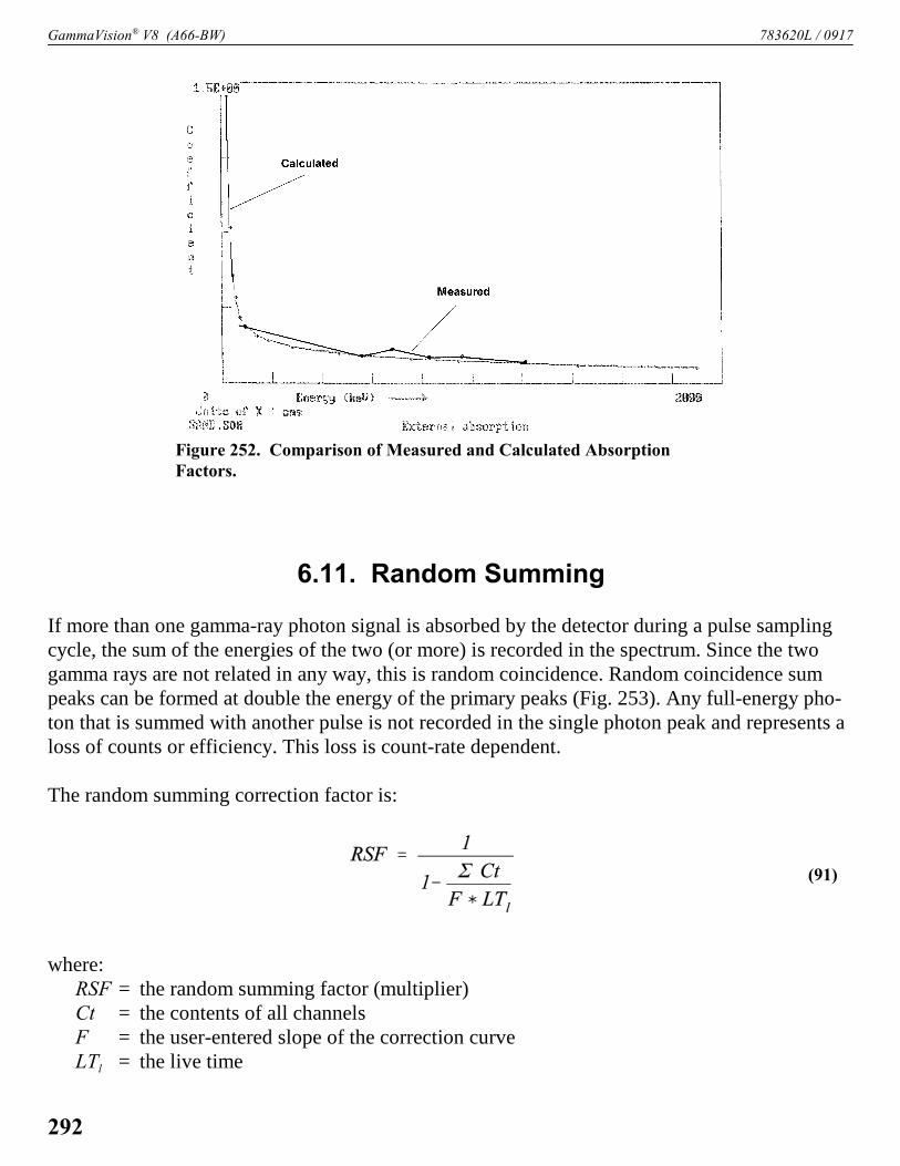
GammaVision® V8 (A66-BW) 783620L / 0917
Figure 252. Comparison of Measured and Calculated AbsorptionFactors.
(91)
6.11. Random Summing
If more than one gamma-ray photon signal is absorbed by the detector during a pulse samplingcycle, the sum of the energies of the two (or more) is recorded in the spectrum. Since the twogamma rays are not related in any way, this is random coincidence. Random coincidence sumpeaks can be formed at double the energy of the primary peaks (Fig. 253). Any full-energy pho-ton that is summed with another pulse is not recorded in the single photon peak and represents aloss of counts or efficiency. This loss is count-rate dependent.
The random summing correction factor is:
where:RSF = the random summing factor (multiplier)Ct = the contents of all channelsF = the user-entered slope of the correction curveLTl = the live time
292

783620L / 0917 6. ANALYSIS METHODS
Figure 253. Random Summing. The Sum Peak Is the Sum of TwoCoincident Low Full-Energy Peaks.
This value is set to 1.0 if it is calculated at less than or equal to zero.
6.11.1. Random Summing Correction
The uncorrected peak area is multiplied by RSF to obtain the corrected peak area. This is donebefore the peak area is converted to activity.
The slope of the correction curve is dependent on the detector and the source/detector geometry.It is experimentally determined by the following simple procedure. The procedure requires tworadioactive sources: one of low activity and high energy, and one of high activity and a lowerenergy. The energy of the high-activity source must be chosen so that it will not interfere withthe high-energy peak, i.e., it should be less than half the energy. Two such sources are 88Y and137Cs.
Position the high-energy source in front of the detector so that the count rate is low and collect aspectrum with a small counting statistical error (e.g., 100000 counts in the peak area). Measurethe net peak area of the high energy gamma ray and the total counts in the spectrum (seeSection 5.4.3, Calculate/Peak Info...). Now position the low-energy source in front of the detec-tor to increase the count rate and collect a second spectrum for the same live time as the firstspectrum. Again measure the net peak area and total counts in the spectrum. More spectra can becollected by moving the low-energy source closer to the detector to increase the count rate.
For example, six spectra were collected and the results are shown in Table 14.
293

GammaVision® V8 (A66-BW) 783620L / 0917
Count Rate Peak Area Ratio
200 100000 1.00
2000 98850 0.98
4000 97200 0.97
6200 95900 0.95
8000 94800 0.94
9500 93700 0.937
Table 14. Random Summing Data.
(92)
(93)
Using the lowest and highest count rate values, the slope is calculated as:
The negative of this slope is the factor you enter as the Random Summing factor on the Sampletab under Analyze/Settings/Sample Type....
6.12. Reported Uncertainty
The uncertainty printed on the report can be either counting or total uncertainty. They can beprinted at 1, 2, or 3 sigma. The counting uncertainty is the uncertainty of the peak area due tostatistical uncertainty, and was discussed earlier. For a peak net area, the counting uncertaintycan be expressed in percent of the peak area. This same percent is used to express the percentcounting uncertainty in the activity values.
6.12.1. Total Uncertainty Estimate
The total uncertainty estimate (1 sigma) is determined by summing in quadrature the individualuncertainties from the various analysis components.
294

783620L / 0917 6. ANALYSIS METHODS
(94)
where:ócount = counting uncertainty estimate (Section 6.3.4). If PBC is enabled, this term
includes the PBC uncertainty calculated per Section 6.12.12.ónor = additional normally distributed uncertainty estimate (Section 6.12.3)órsum = random summing uncertainty estimate (Section 6.12.4)óabs = absorption uncertainty estimate (Section 6.12.5)ónuc = nuclide uncertainty estimate (Section 6.12.6)óeff
= efficiency uncertainty estimate (Section 6.12.7)ógeo = geometry uncertainty estimate (Section 6.12.8)ósys = systematic (uniformly distributed) uncertainty estimate (Section 6.12.9)óadl = additional user-defined uncertainty factor (Section 6.12.10)ós = sample size uncertainty (Section 6.12.11)
All components of uncertainty estimates except óuni are computed at the 1-sigma level. Theuncertainty estimate for a uniformly distributed error is used at the full range. If a correction fac-tor is not used, the uncertainty estimate is zero for that component.
6.12.2. Counting Uncertainty Estimate
This is discussed in Section 6.3.4.
6.12.3. Additional Normally Distributed Uncertainty Estimate
Inputnor is obtained based on the Random setting in the Additional Error section of theAnalysis tab.
where:ó2
nor = variance of additional normally distributed uncertainty (% 1 sigma)Inputnor = user input for normally distributed uncertainty (% 1 sigma)
295

GammaVision® V8 (A66-BW) 783620L / 0917
(95)
(96)
(97)
6.12.4. Random Summing Uncertainty Estimate
where:ó2
rsum = variance of random summing error estimateCFrs = random summing correction factor
6.12.5. Absorption Uncertainty Estimate
where:ó2
abs = variance of attenuation error estimateCFab = absorption correction factor
6.12.6. Nuclide Uncertainty Estimate
where:ó2
nuc = variance of nuclide error estimateInputnuc = user uncertainty input for nuclide (% 2 sigma). This is the uncertainty in the yield
(branching ratio) for the first gamma ray in the library for each nuclide.
6.12.7. Efficiency Uncertainty Estimate
The efficiency uncertainty is computed differently depending on the type of fit used for theefficiency calculation. The components used for efficiency include the errors due to uncertaintyof the calibration source, uncertainty of the calibration fit, and the counting uncertainty of thecalibration.
296

783620L / 0917 6. ANALYSIS METHODS
(98)
(99)
(100
(101)
The total efficiency uncertainty, óeff, is calculated as:
where óc is the calibration fit uncertainty and óp is the calibration counting uncertainty, bothdiscussed in the sections below.
6.12.7.1. Calibration Counting Uncertainty
When an efficiency calibration is performed, the counting uncertainty is calculated and stored inthe calibration record. In general, there is an above-the-knee counting uncertainty and a below-the-knee counting uncertainty, both calculated and saved to the calibration data record.
For polynomial and TCC-polynomial type calibrations, the counting uncertainty above the kneeis calculated as the averaged counting uncertainty of all calibration peaks involved, regardless ofthe knee energy, as shown below:
where óci is the counting uncertainty of the i-th calibration peak, and N is the total number ofcalibration peaks used. The counting uncertainty below the knee is always set to zero for thesetwo calibration types:
For all other calibration types, the above-the-knee counting uncertainty is calculated as theaveraged counting uncertainty of all the calibration peaks with energy greater than or equal tothe knee energy, as shown below:
where N1 isthe number of calibration peaks whose energies are greater than or equal to the kneeenergy.
The below-the-knee counting uncertainty is calculated as the averaged counting uncertainty ofall the calibration peaks with energy less than the knee energy:
297

GammaVision® V8 (A66-BW) 783620L / 0917
(102)
(103)
(104)
(105)
where N2 is the number of calibration peaks with energies less than the knee energy. If N2 iszero, the counting uncertainty is zero.
For polynomial and TCC-polynomial type calibrations, the calibration counting uncertainty óp isalways equal to the counting uncertainty above the knee:
For all other calibration types, óp is calculated as:
NOTE For calibrations performed before GammaVision 7, the above-and below-the-kneecounting uncertainties are both zero. To take into account the counting uncertaintydiscussed here, update the efficiency calibration with GammaVision 7 so the newuncertainties will be calculated and stored in the calibration file. Then, when a spec-trum is analyzed, the final reported activity uncertainty will take into account theadded uncertainty in calibration.
6.12.7.2. TCC-Polynomial
The calibration variance is the averaged variance of all the calibration points in the certificatefile:
where:óC = the calibration uncertaintyói = the uncertainty of the ith calibration point from the certificateN = the total number of calibration points
6.12.7.3. Interpolative
298

783620L / 0917 6. ANALYSIS METHODS
(106)
(107)
For this calculation, the calibration points are sorted in ascending order by energy. If energy E isless than the first (lowest-energy) calibration point, Ei and Ei+1 are the two lowest-energy calibra
tion points. If energy E is greater than the last (highest-energy) calibration point, Ei and Ei+1 arethe two highest-energy calibration points. For all other cases, Ei < E < Ei+1 :
where:ói = the uncertainty (not the fractional uncertainty) associated with energy Ei from the
certificate.
This calculation is also used when energy E is less than the first calibration point, the efficiencyfit is polynomial, and the detector is N-type.
6.12.7.4. Linear, Quadratic or Polynomial
In general, the efficiency curve (or efficiency fit) can be expressed as:
where:å = the efficiency at energy Eak = the kth fitting parameter
299

GammaVision® V8 (A66-BW) 783620L / 0917
(108)
(109)
The parameters x, n, and m depend on the type of efficiency curves:
! For linear/quadratic fits:
! For polynomial fits:
If the energy x is lower than the lowest two calibration points, the analysis engine performs aninterpolated fit instead of a polynomial fit. The summation in Eq. 107 is the sum over all thefitting parameters, k = 1, ..., m, not the sum over all the calibration points.
300

783620L / 0917 6. ANALYSIS METHODS
(110)
(111)
(112)
(113)
(114)
Now let us define a parameter y as y = ln å. This yields:
The fitted efficiency at any point xi (as defined in Eqs. 108 and 109 above) is:
Matrix Solution
Equation 111 above is Eq. 7.12 in Bevington,34 except that the function fk (xi ) has been replacedby xi
n, a particular type of polynomial:
where xi and n are defined in Eqs. 108 and 109.
From Eq. 7.14 in Bevington, the â matrix is calculated using Eq. 112 above:
where ói and N are defined in Eq. 105, yi is defined in Eq. 111, and xi is defined in Eqs. 108and 109.
From Eq. 7.15 in Bevington, the á matrix is calculated by:
where for a linear/quadratic fit:n1 = n ! 1k1 = k ! 1
and for a polynomial fit:n1 = 2 ! nk1 = 2 ! k
34Bevington, Philip R. and D. K. Robinson. Data Reduction and Error Analysis for the Physical Sciences, 2nded., McGraw-Hill, 1992.
301

GammaVision® V8 (A66-BW) 783620L / 0917
(115)
(116)
(117)
(118)
The ói factor is the fractional uncertainty at the ith calibration point (as defined for Eq. 105). ói isnot the absolute uncertainty because the actual curve being fitted is not the efficiencies them-selves but the natural log of the curve.
Matrix Inversion
From Eq. 7.20 in Bevington, the nth fitting parameter in our Eq. 110 or Eq. 107 can be calculatedas:
where ä is the inverse matrix of á:
The ä matrix is called the error matrix because its diagonal elements are the variances of the fit-ting parameters, and the off-diagonal elements are the covariances of the fitting parameters (seeEq. 7.25 in Bevington):
If i = j, is the variance for the fitting parameter ai. If i � j, is the covariance between
the fitting parameter ai and aj.
Uncertainty of the Fit
From Eq. 3.13 in Bevington, the polynomial fit uncertainty is given by:
where y is the polynomial given in Eq. 110 and ai is the ith fitting parameter. The error matrix äi j
has been used instead of for clarity. Equation 118 does not use the factor 2 before the
covariance terms, as is done in Bevington Eq. 3.13. This is due to the double-summationnotation used in Eq. 118 and because the error matrix is symmetric (ä12 = ä21, ...). The diagonal
elements are not double-counted in the above equation. (In Bevington Eq. 3.13, is denoted
as .)
302

783620L / 0917 6. ANALYSIS METHODS
(120)
(121)
(122)
(123)
(119)
From Eq. 110, since , we have:
where for a linear/quadratic fit:i1 = i ! 1j1 = j ! 1
and for a polynomial fit:i1 = 2 ! ij1 = 2 ! j
Finally, the calibration uncertainty is:
where å is the fitted efficiency at energy E (from Eq. 107), and óy is calculated from Eq. 119. Ifóc is zero, then the “sigma above” (óa) or “sigma below” (ób) value described in the followingparagraphs is used.
If the fit type is neither polynomial nor TCC-polynomial, the calibration uncertainty is calculatedas:
where óa and ób are defined as follows.
If the energy E > Eknee ,
303

GammaVision® V8 (A66-BW) 783620L / 0917
(126)
(125)
(124)
If E # Eknee,
where:åi = the measured efficiency at energy Ei
fi = the calculated efficiency at Ei from Eq. 107Eknee = the efficiency knee energy
Na is the number of efficiency points above the knee energy and Nb is the number of efficiencypoints below the knee energy. Both Na and Nb must be greater than 1. If óa or ób is zero, thedefault uncertainty of 1.5% is used.
If the fit type is polynomial but not TCC-polynomial, the calibration uncertainty is calculated as:
For polynomial fits, Eknee is always ignored.
Sometimes, the efficiency pairs might be missing from the calibration file but the fit parametersand fit type are stored in the file. In these cases, the óa or ób value is used.
6.12.8. Geometry Uncertainty Estimate
This value, ógeo2,.is based on the geometry uncertainty estimate entered on the geometry correc-
tion sidebar (Fig. 153):
If the uncertainty is 0 or no value is entered, or if using a .GEO file from an earlier version ofGammaVision, a fixed value of 1.5% is used.
304

783620L / 0917 6. ANALYSIS METHODS
(127)
(128)
(129)
6.12.9. Uniformly Distributed Uncertainty Estimate
This is based on the Systematic error entered on the System tab and saved in the .SDF file.
where:ó2
sys = uncertainty estimate for a uniformly distributed uncertainty estimateInputsys = user input for full range (%)
6.12.10. Additional User-Defined Uncertainty Factors
On the Uncertainties tab (Fig. 144) you can optionally define up to nine uncertainty values óusr1
through óusr9, which are added quadratically to the total relative uncertainty, ót, as the additionaluser-defined uncertainty factor óadl as follows:
Both the field description and its corresponding non-zero value must be defined for an uncer-tainty entry or it is not used. These values are stored in the .SDF file as well as .SPC spectrumfiles, and are reported individually in the Analysis Parameters table.
6.12.11. Sample Size Uncertainty
The value ós2 is based on the sample size uncertainty entered on the System tab.
If using an .SDF file from an earlier version of GammaVision, a fixed value of 1.5% is used.
305

GammaVision® V8 (A66-BW) 783620L / 0917
(130)
(131)
(132)
(133)
(134)
6.12.12. Peaked Background Correction and Uncertainty Calculations
6.12.12.1. Single PBC Subtraction
If the PBC net count rate at energy E is Rp (in cps), the live time is LT (in seconds), and the frac-tional uncertainty of the net PBC peak count rate is óp, then the corresponding PBC counts Np
and the associated absolute uncertainty óabsp in counts can be calculated from the following:
If N0 is the peak area in counts before PBC, ó0 is the corresponding fractional uncertainty, andóabs0 is the corresponding absolute uncertainty for the net peak area before PBC (see Eq. 48,page 250), the absolute peak area uncertainty before PBC is:
The PBC corrected peak area N (in counts) is calculated as:
If, after PBC, the net peak area is <0, it is set to 0 unless Directed Fit is enabled (because nega-tive peak area is not physical). After PBC, the subtracted PBC area is added to the peak back-ground. If B0 is the peak background before PBC, the peak background after PBC is:
After PBC, the variance of the peak net area counts has contributions from the PBC subtractionas well as from the change in the peak background discussed above. The variance from the PBCsubtraction is simply óabsp
2.
306

783620L / 0917 6. ANALYSIS METHODS
(135)
(136)
(137)
(138)
The variance due to the change in the peak background is taken to be the increase in the peakbackground, Np. Therefore, after PBC, the total absolute uncertainty (in counts) for the net peakarea is calculated as:
Note that for PBC, only the absolute uncertainties (not relative) are added in quadrature. Afterthe PBC correction, the relative uncertainty in percent is calculated as:
If the PBC corrected area is exactly zero, the relative uncertainty is set at 1000% (or 10.0), thedefault value used in all cases where the activity is zero.
Note that when PBC is enabled, the counting uncertainty for a peak always has PBC contribu-tions. That is, the counting uncertainty calculated before PBC (ó0 in Eq. 132) is not saved in the.UFO file. The same holds for the peak area; it is always the PBC corrected value, and the netpeak area before PBC is not saved in the .UFO file.
6.12.12.2. Multiple PBC Subtraction
If there are multiple PBC peaks under a peak, that peak is subject to multiple PBC subtractions.The sum of the PBC net areas is simply the sum of individual PBC areas (for comparison, seeEq. 130 for single PBC subtraction):
where LT is the live time, Rp_i is the PBC count rate for the i-th PBC, and m is the total numberof PBC peaks.
The total PBC uncertainty is calculated from the following (compare to Eq. 131):
where óabsp_i is the absolute uncertainty of each PBC peak in counts. After calculating Np and óabsp
for the combined PBC subtraction with multiple PBC the rest of the calculations can be appliedthe same way as for a single PBC (that is, all equations in this section except Eqs. 130 and 131can be applied the same way for both single and multiple PBC subtractions).
307

GammaVision® V8 (A66-BW) 783620L / 0917
(139)
6.13. EBAR — Average Energy
The average energy calculation (EBAR) represents the sum of the average beta-gamma emissionenergy per disintegration for the identified radionuclides in the sample. The nuclides must be inthe analysis library and the EBAR table (i.e., the .EBR file). The weighting factors of the activityof each isotope are usually defined by the plant chemistry procedures or can be calculated basedon data found in radioactive-decay tabulations such as DOE/TIC-1102635 or ORNL/NUREG/TM-102.36
The EBAR formula is:
where:EBAR = the sum of the average beta and gamma energies in keV/disintegrationEi = , the average energy/disintegration for an individual nuclideAi = the activity for nuclide in = the number of nuclides
The average energy for a given nuclide is the sum of the product of the energy of the gamma rayand the abundance of that ray, plus the product of the energies of the electrons (1/3 the maxi-mum for beta decay), plus the abundance of that ray.
As an example, consider the decay scheme for 133Xe–133Cs in Fig. 254.
The maximum beta energy is given as 346 keV, which gives 267 keV and 45 keV for theenergies of the transitions to the 160 keV and 382 keV states in 133Cs. In addition to beta-decayelectrons, the internal conversion electrons must also be included. The K-conversion electronhas an energy of 45 keV and an abundance of 54%; the L electron has an energy of 75 keV andan abundance of 7%.
35DOE/TIC-11026, United States Department of Energy, Office of Scientific and Technical Information, OakRidge, Tennessee.
36Technical Manual TM-102, Nuclear Regulatory Commission Guide, Oak Ridge National Laboratory, OakRidge, Tennessee.
308

783620L / 0917 6. ANALYSIS METHODS
Figure 254. Decay Scheme.
Thus, for the betas, the energy is:
346 × 0.993 × 1/3 = 114.5+ 267 × 0.007 × 1/3 = 1.9 0.6+ 45 × 6.0×10-5 × 1/3 = 0+ 45 × 0.534 = 24.1+ 45 × 0.09 = 6.8
146.0
For the gamma rays, each gamma energy is multiplied by its abundance. In addition, the x-rayfluorescence from the internal conversion must also be included. For the two electrons (Kand L), the x-ray energies are 36 keV and 6 keV, respectively. The same abundances as aboveare used.
309
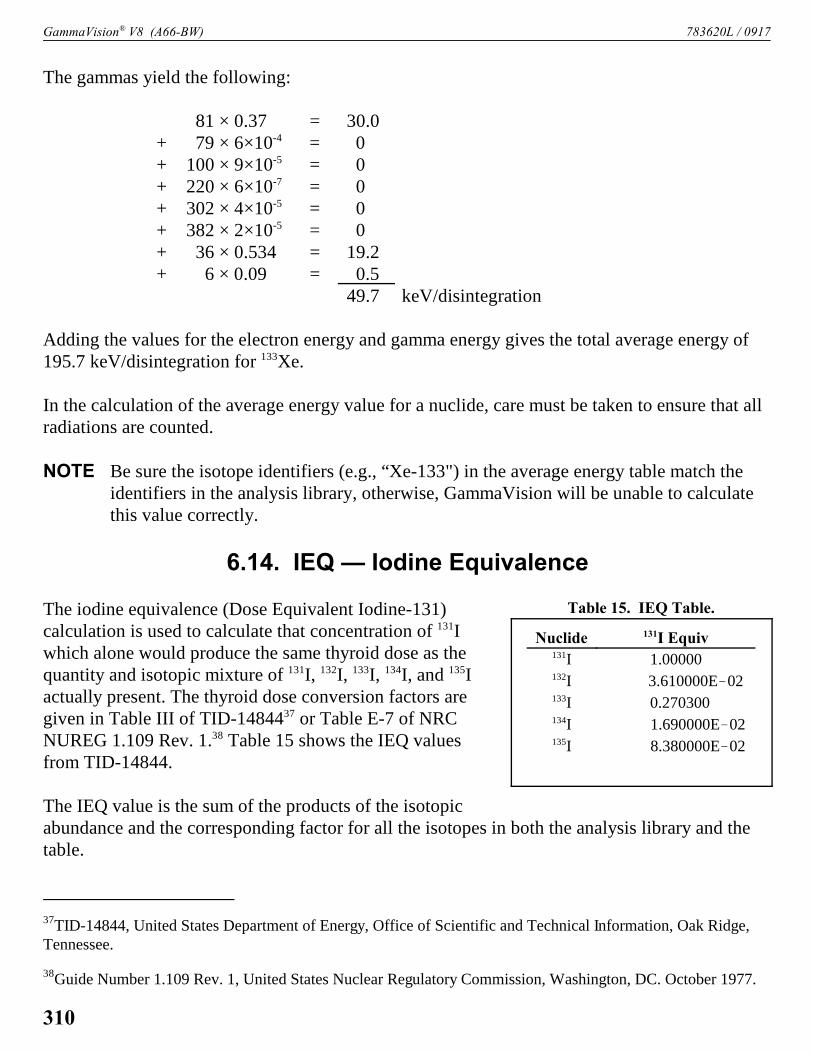
GammaVision® V8 (A66-BW) 783620L / 0917
Nuclide 131I Equiv131I 1.00000132I 3.610000E!02133I 0.270300134I 1.690000E!02135I 8.380000E!02
Table 15. IEQ Table.
The gammas yield the following:
81 × 0.37 = 30.0+ 79 × 6×10-4 = 0+ 100 × 9×10-5 = 0+ 220 × 6×10-7 = 0+ 302 × 4×10-5 = 0+ 382 × 2×10-5 = 0+ 36 × 0.534 = 19.2+ 6 × 0.09 = 0.5
49.7 keV/disintegration
Adding the values for the electron energy and gamma energy gives the total average energy of195.7 keV/disintegration for 133Xe.
In the calculation of the average energy value for a nuclide, care must be taken to ensure that allradiations are counted.
NOTE Be sure the isotope identifiers (e.g., “Xe-133") in the average energy table match theidentifiers in the analysis library, otherwise, GammaVision will be unable to calculatethis value correctly.
6.14. IEQ — Iodine Equivalence
The iodine equivalence (Dose Equivalent Iodine-131)calculation is used to calculate that concentration of 131Iwhich alone would produce the same thyroid dose as thequantity and isotopic mixture of 131I, 132I, 133I, 134I, and 135Iactually present. The thyroid dose conversion factors aregiven in Table III of TID-1484437 or Table E-7 of NRCNUREG 1.109 Rev. 1.38 Table 15 shows the IEQ valuesfrom TID-14844.
The IEQ value is the sum of the products of the isotopicabundance and the corresponding factor for all the isotopes in both the analysis library and thetable.
37TID-14844, United States Department of Energy, Office of Scientific and Technical Information, Oak Ridge,Tennessee.
38Guide Number 1.109 Rev. 1, United States Nuclear Regulatory Commission, Washington, DC. October 1977.
310

783620L / 0917 6. ANALYSIS METHODS
(140)
(141)
The value is:
where:Ai = the activity for the ith isotopeFi = the ith factorl = all the isotopes
The units of IEQ are the units specified in the report. If decay correction is specified, both thedecay-corrected equivalent activity and the time-of-count equivalent activity are reported.Isotopes that are not found (those whose MDAs are reported) are not included in the reportedvalue. If the decay correction is more than 12 half-lives, the decay-corrected value is notincluded in the reported value.
NOTE Be sure the isotope identifiers (e.g., “I-133") in the average energy table match theidentifiers in the analysis library, otherwise, GammaVision will be unable to calculatethis value correctly.
6.15. DAC or MPC
The DAC or MPC calculation is a measure of the fraction of the allowed activity or concentra-tion in the current sample. The allowed activity or concentration values are stored in a table (seeSection 5.5.1.8). A value of 1 (or 100%) means the sample had 100% of the allowed value.
NOTE Be sure the isotope identifiers (e.g., “Xe-133") in the table match the identifiers in theanalysis library, otherwise, GammaVision will be unable to calculate this valuecorrectly.
For cases where nuclides are identified in the analysis but not explicitly included in the DACtable, you can optionally add a nuclide named “Default” with an associated DAC value to theDAC table for use in the calculation. If no “Default” entry is included, then nuclides withactivity reported that do not match a nuclide name in the DAC table will not affect the DACcalculation.
The value is defined as:
311

GammaVision® V8 (A66-BW) 783620L / 0917
312

783620L / 0917 6. ANALYSIS METHODS
Figure 255. 60Co Decay to 60Ni.
where:Ai = the activity of isotope iDi = the allowed value for isotope iDAC = the fractional allowed value in percent
The value is not calculated for MDA values.
6.16. True Coincidence Correction
In the case where a nuclide emits multiple cascadegamma rays when it decays, these multiple gamma rayscan be detected individually or together as one gammaray. An example decay is 60Co, as shown in Fig. 255.The two gamma rays (1173.2 and 1332.5 keV) areemitted in cascade or one after another. The lifetime ofthe intermediate state is very short so that it appearsthat the two gamma rays are emitted in coincidence(i.e., at the same time). Since the two gamma rays caninteract in the detector in a time short compared to the response time of the detector and theresolving time of the electronics, the two gamma rays are recorded as a single gamma ray.
When the two gamma rays are detected as one, it effects the spectrum in two ways. One way isthe creation of a “sum” peak that is the sum of the amplitudes of the two individual full-energypeaks. The second way is to remove counts from the full-energy peak. The first creates extrapeaks in the spectrum. The second reduces the peak area of these gamma rays and thus thereported activity of the nuclide.
The reduction of the peak area due to summing is more important than the creation of the “sumpeak.” The sum peak requires the addition of two full-energy pulses to get the summed energy.The reduction of the peak area only requires that there be a full-energy interaction at the sametime as another interaction from the other members of the cascade. Recall that most of the inter-actions in the detector do not produce full-energy peaks, but produce partial-energy interactions(the Compton background). A summing with any of the partial-energy signals will result in thefull-energy pulse being removed from the full-energy peak. Further details can be found in manyreferences.39,40,41
39 Glenn F. Knoll, Radiation Detection and Measurement, 3rd edition, p. 323, Wiley and Sons, 2000.
40 Gilmore, G., and J.D. Hemingway, Practical Gamma-Ray Spectrometry, p. 156, Wiley and Sons, 1995.
41 “Calibration and use of Germanium Spectrometers for the measurement of gamma-ray emission rates ofradionuclides,” ANSI N42.14-1991.
313

GammaVision® V8 (A66-BW) 783620L / 0917
(142)
(143)
The true coincidence correction (TCC) is the correction necessary to account for all of thepulses removed from the full-energy peak. This correction is a simple divisor of the net peakarea, that is the net peak area is increased by the correction factor. The correction factor is detec-tor and sample geometry dependent. The correction factor depends on the full-energy efficiency,that is the ability of the detector to detect the total energy of the gamma ray, and the total effi-ciency, that is the ability of the detector to detect any part of the gamma ray energy. The full-peak efficiency is determined in the efficiency calibration (Calibrate/Efficiency) and the totalefficiency is determined in the TCC part of Calibrate/Calibration Wizard....
6.17. ISO NORM Implementation in GammaVision
This section details the implementation of the ISO-11929:2010 standard referred to as ISONORM in GammaVision.
6.17.1. The ISO NORM Model in GammaVision
The ISO NORM model is described mathematically as:
where:y = peak activity (A)x1 = gross counts (G)x2 = background counts (B)x3 = shielding factor (egual to 1 in GammaVision)x4 = additional background correction term (zero in GammaVision)î = conversion factor from net counts to activity as described in Equation 60.
This formula simplifies to A=N * î which is described in Equation 59.
6.17.2. Peak Calculation Details
6.17.2.1. Critical Level or Decision Threshold
Critical peak area NCL is calculated as follows when Net Counts is presumed to be zero:
314

783620L / 0917 6. ANALYSIS METHODS
(144)
(145)
(146)
(147)
(148)
(149)
where:k1-á is the quantile of the normal distribution for the probability á
If the uncertainty of the background is taken as the square root of the peak background, and if k1-
á is 1.645, then the ISO NORM Critical Level calculation is similar to the Critical Level MDAMethod (Section 6.9.2.2):
6.17.2.2. Peak MDA or Peak Detection Limit
ISO NORM MDA is calculated as follows:
where:
Uncertainties in the MDA Equation
The uncertainty of the conversion factor takes into account all of the total uncertainty parameterswithout the counting uncertainty term:
where:óA = Peak Activity total uncertainty (Section 6.12). ócount = Peak Counting uncertainty (Section 6.3.4)
315

GammaVision® V8 (A66-BW) 783620L / 0917
(150)
(151)
(152)
(153)
(154)
(155)
Special Cases
Under special conditions when both error probabilities are the same:
So, the MDA is:
If we further assume the error probability is at 5% and the variance of the background is back-ground B itself:
then the MDA is as follows (similar to MDA Method 12 which is derived from Currie):
MDA to Critical Level Ratio
When the critical level, in counts, is much greater than k1-á2, the MDA can be calculated from the
following equation:
where f is defined as:
316

783620L / 0917 6. ANALYSIS METHODS
(156)
(157)
(158)
(159)
(160)
(161)
If we define the above MDA ratio as R:
and define X and A as:
then the MDA ratio R becomes:
For a given R and A, the corresponding f can be obtained as follows:
If the beta risk error and the alpha risk error are the same (k1-á = k1-â = k), then no matter thevalue of k and the uncertainty, R is twice the value of factor f:
Maximum MDA Ratio
If the uncertainties are extremely small so that A is very large, then the MDA correction factor fshould be close to 1.0 and the MDA ratio R approaches a value of 2.0. Note that this is true eventhough the beta and alpha errors are not the same. Therefore, the minimum MDA ratio should beset to 2.0 as well. Under typical conditions, the following are true:
However, when the uncertainty is increased, A becomes smaller and f becomes larger such thatthe ratio can approach infinity if the denominator for f is zero (A . 1). When the uncertainty isfurther increased, both f (or R) and the MDA become negative.
317

GammaVision® V8 (A66-BW) 783620L / 0917
(162)
(163)
(164)
The MDA is prevented from going negative or to infinity by reducing the beta risk error so thereis an upper limit for the ratio R:
The steps for limiting the ratio are:
1) Calculate the MDA ratio using the original alpha and beta risk error.
2) If the calculated R is greater than RMax, force the ratio R to the value of RMax to calculate anMDA correction factor fmax as shown below:
3) To reduce the MDA correction to the value fmax, the beta risk error must be increased todecrease the k1-â value. The new beta risk error can be calculated from:
If the upper limit of R is set to 3, the corresponding maximum MDA correction factor is about1.5. In GammaVision, RMax can be any value from 2 to 1000 for the “Maximum ISO NORMMDA Ratio factor” in the b30winds.ini (n30winds.ini for NAI32) file. Any value outside thisrange will result in using the default value of 3.
Maximum MDA Report
If RMax is 3.0, the uncertainty to reach the maximum correction is about 35.1% with all para-meters at default values. When the actual uncertainty is larger than this a new k1-â is calculated sothe MDA ratio R remains at RMax. If the uncertainty is extremely large, the asymptotic value ofk1-â is zero and the corresponding value for the beta risk factor is 50%.
When the maximum MDA ratio has been reached, an “I” flag is reported next to the isotopename as shown here:
AM-241 I 5.7471E+03 6.7293E-01% 6.0850E+01% 1.000E+45.7471E+03 5.6712E+03 5.8230E+03 5.791E+01 6.729E-01%
At the end of the ISO NORM table, the flags are defined as:
I - ISO NORM MDA ratio at maximum for one or more peaks
318

783620L / 0917 6. ANALYSIS METHODS
(165)
(166)
(167)
(168)
Note that the “I” flag supercedes other nuclide flags (A, B, C, F, and H). If there is more than onepeak defined in the library for an isotope, it is possible that the ISO NORM MDA for one peak islimited even though the MDA is not capped for other peaks of the same isotope. But the isotopewould still have the “I” flag assigned. However, if the nuclide is not present and the MDA isreported as the activity, the less-than flag may supercede all other flags, including the “I” flag,since that flag is of higher importance to the users. At default values, the uncertaintycorresponding to the maximum MDA ratio is about 35%. The best estimated uncertainty can beused as an indication of whether the maximum MDA ratio has reached.
6.17.2.3. The Best Estimated Activity
The best estimated activity is calculated as:
where:
and the parameter ù is defined as follows (see Eq. 31 or F.18 in ISO NORM):
The integration is from !4 to Q. In Eq. 165, the second term comes from the biased estimatorused in ISO NORM.
The uncertainty of the best estimated net peak area counts, based on Eq. 34 in ISO NORM, is:
319

GammaVision® V8 (A66-BW) 783620L / 0917
(169)
(170)
where all quantities have been defined before. From Eq. 165, because the best estimated peakarea Nh is always greater than the net peak area N, the uncertainty of the best estimated peak areais always less than the uncertainty of the net peak area. If this value is zero, it is set to the bestestimated net peak area.
If the isotope activity is zero or negative, and if the best estimated activity is more than threetimes the uncertainty of the best estimated activity, the best estimated activity and the associateduncertainty are set to zero.
6.17.2.4. The Lower and Upper Limits of the Activity
From ISO NORM Eq. 29, the lower limit of the peak area is:
All the quantities have been defined earlier except ã, which is related to the confidence intervaland 1!ã is the probability that the measured value is within the confidence limits calculated (thetypical value of ã is 0.05 for 95% confidence).
According to ISO NORM Eq. 30 or F.17, the upper limit of the peak area is:
If the uncertainty is small compared to the net peak area (i.e., when Q is large), then ù is veryclose to 1. Under those conditions, N is in the middle of the confidence limits. When Q is small,kp is less than kq, so N is closer to the lower limit than the upper limit. If the peak area uncertaintyis zero (typically this happens when the net peak area is zero), the lower and upper confidencelimits are set to zero. Conversion from peak area limits to the corresponding activity limits is perEquation 59.
6.17.3. Nuclide Calculation Details
The nuclide activity and its associated uncertainty are the branching-ratio weighted average ofall the “qualifying” peaks of the nuclide (i.e., those that meet the criteria in Section 6.7.1 forinclusion in the average activity calculation). For all ISO NORM quantities (CL, MDA, etc.), ifthose qualifying peaks are found, then the ISO NORM results are also weighted using thebranching ratios. Otherwise, ISO NORM quantities are calculated from the “MDA” line, whichis typically the line used by GammaVision to calculate the MDA in regular analysis reports.
6.17.3.1. Nuclide Activity
The final activity of the nuclide is the average of the peak activity of the qualifying peaks asdescribed in Section 6.7.1.
320

783620L / 0917 6. ANALYSIS METHODS
(171)
(172)
(173)
6.17.3.2. Nuclide Activity Counting Uncertainty
Nuclide Counting Uncertainty is calculated as described in Section 6.7.2.
6.17.3.3. Nuclide Best Estimated Activity
The nuclide best estimated activity is given by:
where Ahi is the best estimated activity for the ith qualifying peak calculated from Eq. 165. If noappropriate peaks are found, the MDA peak is used.
6.17.3.4. Nuclide Best Estimated Activity Uncertainty
The 1-sigma uncertainty of the best estimated nuclide activity is given by:
where óAhi is the uncertainty of the best estimated activity for the ith qualifying peak. If 2 sigma or3 sigma is selected on the Report tab, this value will be multipled respectively by 2 or 3.
6.17.3.5. Nuclide Critical Level
The nuclide critical level is given by:
where ACLi is the critical level of the ith peak.
321

GammaVision® V8 (A66-BW) 783620L / 0917
(174)
(175)
(176)
(177)
6.17.3.6. Nuclide MDA
The nuclide MDA is given by:
where AMDAi is the MDA for the ith qualifying peak.
6.17.3.7. Nuclide Lower and Upper Activity Limits
The lower activity limit is given by:
and the upper activity limit is given by:
where A<i and A>i are the lower and upper activity limit of the ith qualifying peak.
6.17.3.8. Total Reported Activity
Total reported activity represents the summed activity calculated for all nuclides found in thesample. It is calculated as follows and printed in the analysis report immediately after theSummary of Nuclides table, or the Summary of Nuclides (ISO NORM) table if the ISO NORMreport checkbox is marked on the Report tab.
where AAn is the calculated nuclide activity for the n-th nuclide.
322

783620L / 0917 6. ANALYSIS METHODS
(178)
(179)
(180)
Note that if an MDA is reported for AAn for a particular nuclide, that nuclide’s contribution is notincluded in Atot. In addition, any nuclide with the “Activity Not In Total” flag set is alwaysexcluded. Also note that this total activity is typically different from the total activity calculatedfor the standard GammaVision report. This is because the MDA values (which in turn might beused as the nuclide activity values) are calculated differently in ISO NORM due to the differ-ences in background variance calculations.
6.17.4. GammaVision / ISO NORM Unique Calculations
6.17.4.1. Negative Peak Area and Confidence Interval
The ISO NORM standard does not make clear how negative peak areas should be handled. How-ever, it can be shown that for the confidence interval, the peak area can be negative.
Lower Confidence Limit
The lower confidence limit can be rewritten as:
From Eq. 167 it is clear that Q is just kù. Because the probability p is always less than ù, to get asmaller probability, kp (the horizontal axis in Gaussian function) must be less than kù.
Therefore, it can be concluded that no matter the value of Q (positive or negative), the followingis always true:
Upper Confidence Limit
The upper confidence limit, kq, is defined in Eq. 170 (ISO NORM Eq. 30 or F.17). Theprobability q is always greater than p because:
323

GammaVision® V8 (A66-BW) 783620L / 0917
(181)
(182)
(183)
(184)
(185)
(186)
(187)
Calculating the difference of the two limits:
From the Gaussian distribution, if the probability 1 - q is less than the probability p, then kq + kp
should be greater than zero.
Thus, it can be concluded that :
Finally, it can be concluded that even in case of negative peak area, the following is always true:
The Best Estimated Activity
The best estimated activity is calculated from Eq. 165. Because Q = N / óN, Eq. 165 can berewritten as:
The best estimated activity is always positive and the following is true:
Uncertainty of the Best Estimated Activity
If for any reason the uncertainty cannot be calculated (due to negative operand in Eq. 28), óNh
will be set to the maximum best estimated activity uncertainty of 100%.
6.17.4.2. Peak Area Uncertainty
324

783620L / 0917 6. ANALYSIS METHODS
(188)
(189)
(190)
(191)
If the relative peak area uncertainty has been calculated, then the peak area uncertainty is simply:
where Pkunct is the relative peak area uncertainty reported in the GammaVision analysis report.If Pkunct is zero and if the activity uncertainty of the isotope is not zero, then óN is calculated byconverting the activity uncertainty in Bq back to uncertainty in counts:
where óA is the nuclide activity. If óA is still zero, then the gross counts under the peak iscalculated and the area uncertainty determined as:
where G is the gross counts under the peak, and óB2 is the peak background uncertainty.
6.18. EDF Gamma Total Analysis
6.18.1. Geometry (K-Factor) Calculation
1) Measure the background between 100 keV and 2 MeV.
2) Calculate the K coefficient, based on the measurement of a 137Cs source, as follows:
whereK = K coefficientTR = Real time, in secondsAs = Source activity at the time of measurement, in BqAg = Gross area between the chosen range of the source spectrum (100 keV–2 MeV),
in countsAbkg = Gross area between the chosen range of the background spectrum
(100 keV–2 MeV), in counts. Choose the background spectrum on the Gamma
325
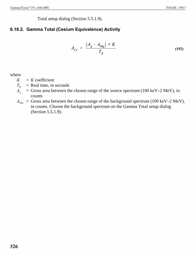
GammaVision® V8 (A66-BW) 783620L / 0917
(192)
Total setup dialog (Section 5.5.1.9).
6.18.2. Gamma Total (Cesium Equivalence) Activity
whereK = K coefficientTR = Real time, in secondsAg = Gross area between the chosen range of the source spectrum (100 keV–2 MeV), in
countsAbkg = Gross area between the chosen range of the background spectrum (100 keV–2 MeV),
in counts. Choose the background spectrum on the Gamma Total setup dialog(Section 5.5.1.9).
326

Figure 256.
7. ANALYSIS REPORT
This chapter covers the contents of the GammaVision analysis report, which is based on theentries in the Sample Type Settings dialog under Analyze/Settings/Sample Type...(Section 5.5.1.1). The report details depend on the analysis engine and setting, spectrum,calibration, and library content, as described below.
7.1. Report Header
The two-line report header (Fig. 256) is repeated on every page.
The first line contains the program name, analysis code in parenthesis (63 in this example),analysis Engine name and version code (ROI32 G70W0.37 in this example), analysis date/time,and page number. The second line contains the Laboratory Name and Spectrum filename.
The analysis code is an integer that defines various conditions applied or encountered during theanalysis. The number is decoded into binary with the following bit usage:
Bit 1 True if the spectrum is energy calibratedBit 2 True if the spectrum is efficiency calibratedBit 3 True if the library is a valid gamma-ray libraryBit 4 True if the isotopic abundance will be reportedBit 5 True if the isotopic matrix will be reportedBit 6 True if the Unidentified Peak Summary, Identified Peak Summary, or Summary
of Library Usage table is reportedBit 7 True if DAC/MPC is enabledBit 8 True if the PBC has been usedBit 9 True if absorption correction is enabledBit 10 True if geometry correction is enabledBit 11 True is peak stripping (library or manual based) is enabledBit 12 True if the directed fit has been enabled
For example, an analysis code of 63 (which is binary 0000 0011 1111, digit numbers read fromright to left) means that the spectrum is (1) energy calibrated, (2) efficiency calibrated, (3) validlibrary found, (4) isotopic abundance is reported, (5) isotope matrix is reported, (6) peak/energymatrix is reported, (8) PBC not used, and (12) Directed Fit not used.
327

GammaVision® V8 (A66-BW) 783620L / 0917
Figure 257.
Normally, this code just confirms that the proper analysis was performed, but it can be usefulwhen troubleshooting a particular analysis when the reported results are not as expected.
7.2. Sample, Detector, and Acquisition Parameters
The first four sections of the report (Fig. 257) contain the sample description; the full path to thespectrum; acquisition information including the start date/time, live time, real time, and deadtime.
The Sample Description may include two lines of text as entered in the Sample Description fieldbefore analyzing the spectrum. The Detector Description is displayed under the Detector Systemheading.
7.3. Calibration Parameters
This section (Fig. 258) includes the calibration filename, internal description from the calibrationfile, efficiency calibration uncertainty, and the energy and efficiency calibration date/time andformula coefficients. The particular coefficients displayed for the efficiency calibration dependon the calibration type and knee settings (where applicable). Refer to Section 5.3 for detailsabout efficiency calibration formulas and respective coefficients.
328

783620L / 0917 7. ANALYSIS REPORT
Figure 258.
Figure 259.
7.4. Library Parameters
This section (Fig. 259) displays the libraries used for analysis and the Library Match Widthsetting.
If Manual Based Peak Stripping is enabled on the Analysis tab, the Second Library specifiedon the Analysis tab is identified on the report as the “Stripping library,” and the Third Libraryspecified on the Analysis tab is identified as the “Second analysis library.” The primary purposeof the stripping library is to define the interference while the second analysis library defineswhich nuclides are assigned the remaining peak area after peak stripping is applied. The strip-ping and second analysis libraries are omitted from the report if Manual Based Peak Strippingis not enabled. Refer to Section 6.5.5.2 for more information on peak stripping.
7.5. Analysis Parameters
This section (Fig. 260) displays various analysis parameters used for the analysis, with theclarifications below.
329
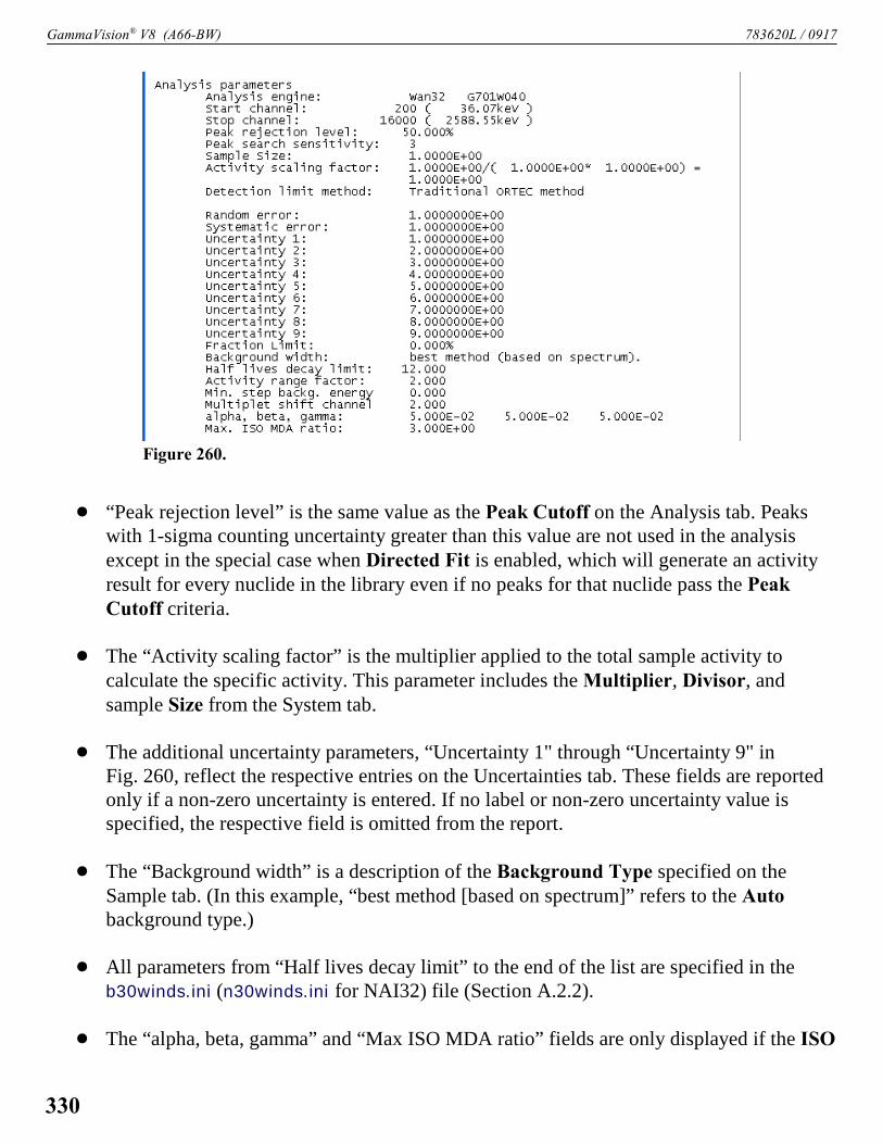
GammaVision® V8 (A66-BW) 783620L / 0917
Figure 260.
! “Peak rejection level” is the same value as the Peak Cutoff on the Analysis tab. Peakswith 1-sigma counting uncertainty greater than this value are not used in the analysisexcept in the special case when Directed Fit is enabled, which will generate an activityresult for every nuclide in the library even if no peaks for that nuclide pass the PeakCutoff criteria.
! The “Activity scaling factor” is the multiplier applied to the total sample activity tocalculate the specific activity. This parameter includes the Multiplier, Divisor, andsample Size from the System tab.
! The additional uncertainty parameters, “Uncertainty 1" through “Uncertainty 9" inFig. 260, reflect the respective entries on the Uncertainties tab. These fields are reportedonly if a non-zero uncertainty is entered. If no label or non-zero uncertainty value isspecified, the respective field is omitted from the report.
! The “Background width” is a description of the Background Type specified on theSample tab. (In this example, “best method [based on spectrum]” refers to the Autobackground type.)
! All parameters from “Half lives decay limit” to the end of the list are specified in theb30winds.ini (n30winds.ini for NAI32) file (Section A.2.2).
! The “alpha, beta, gamma” and “Max ISO MDA ratio” fields are only displayed if the ISO
330

783620L / 0917 7. ANALYSIS REPORT
Figure 261.
NORM section of the report is enabled on the Report tab.
7.6. Correction Parameters
This section (Fig. 261) displays the corrections applied during the analysis for decay,coincidence and random summing, geometry and attenuation/absorption, peak background, andautomatic energy recalibration (if enabled). The Status column displays a “YES” when acorrection is enabled, followed by additional information related to the correction in the“Comments” column. The Status is listed as “NO” for disabled corrections.
! “Decay correct to date” should normally be set to the “Decay during collection” end timeif both are enabled on the Decay tab.
! “Decay during collection” displays the collection start and stop date/time.
! “Peaked background correction” displays the PBC file name entered on the Correctionstab and the date/time the file was created.
! Absorption displays either database information as shown in Fig. 261 (material, densityor mass, internal or external, and scaling factor [the latter is the Length value entered onthe Corrections tab]) or the file information (file name, date/time created, .UFO file name
331

GammaVision® V8 (A66-BW) 783620L / 0917
used to generate the attenuation table, and the scaling factor [again, the Length valueentered on the Corrections tab]).
! “Random summing” displays the slope value entered in the Random Summing field onthe Sample tab; and the Net factor, which is the Random Summing Factor calculated perSection 6.11.
! The “Iodine equivalence” and “Average energy” fields are only displayed if these optionsare enabled on the Isotopes tab.
! The “Energy Calibration” section displays the “Normalized difference,” a measure ofhow well the spectrum peak energies match those in the library (see Section 6.3.6). Thiscan range from 0.0 to 1.0, with 0.0 being the best and 1.0 the worst. High values may bedue to a poor calibration or to analyzing very small peaks that do not have statisticallygood shape. If the automatic energy recalibration is enabled and the criteria specified inSection 6.3.6 are satisfied, a message indicates that the energy calibration was changed tofit the spectrum, and the new energy calibration coefficients used for the analysis aredisplayed.
7.7. Peak and Nuclide Tables
This section covers the various peak and nuclide tables GammaVision can report, based on theanalysis engine used; see the following table. The content of a particular table may vary depend-ing on the settings in the Sample Type Settings dialog or (.SDF) file, and in the b30winds.ini
(n30winds.ini for NAI32) analysis parameters file, which is discussed in detail in Section A.2.2.
Section / Peak or Nuclide Table Analysis Engine
ENV32, NPP32, NAI32 WAN32 ROI32 GAM32
7.7.1 ROI Peak Summary T
7.7.2 Summary of ROI Peak Usage T
7.7.3 Summary of ROI Nuclides T
7.7.4 Background Correction T T T T
7.7.5 Summary of Peaks in Range T
7.7.6 Unidentified Peak Summary T T T T
7.7.7 Identified Peak Summary T T T T
7.7.8 Summary of Library Peak Usage T T T T
7.7.9 Discarded Isotope Peaks T T T
7.7.10 Summary of Discarded Peaks T T T T
7.7.11 Summary of Nuclides in Sample T T T T
332

783620L / 0917 7. ANALYSIS REPORT
Section / Peak or Nuclide Table Analysis Engine
ENV32, NPP32, NAI32 WAN32 ROI32 GAM32
Figure 262.
7.7.12 Summary of Nuclides (ISO-NORM) T T T T
7.7.13 Iodine Equivalence and Average Energy T T T T
7.7.14 DAC Table T T T T
7.7.1. ROI Peak Summary (ROI32 Engine Only)
This table (Fig. 262) displays information for ROIs marked in the spectrum, with the clarifica-tions below.
! ROI parameters are calculated per Section 6.2.1.5.
! Peaks in this table are arranged in ascending energy order based on ROIs marked in thespectrum when the analysis is run.
! Only ROIs with calculated uncertainty lower than the peak cutoff are included in thetable.
! If the peak centroid cannot be calculated, then the peak channel is set to 0 (zero).
! The peak centroid energy is listed in units of keV.
! Peak flags are displayed to the right of the FWHM column. The designators for Deconvo-lution, Shape, and Multiplets (as applicable) can be modified in the b30winds.ini
(n30winds.ini for NAI32) file.
333

GammaVision® V8 (A66-BW) 783620L / 0917
Figure 263.
Figure 264.
7.7.2. Summary of ROI Peak Usage (ROI32 Engine Only)
The content of this table (Fig. 263) is similar to the Summary of Library Peak Usage tabledescribed in Section 7.7.8, except that the analysis data are related only to peaks identified byROIs marked in the spectrum. See Section 7.7.8 for a complete explanation of this table content.
7.7.3. Summary of ROI Nuclides (ROI32 Engine Only)
The content of this table is similar to the Summary of Nuclides in Sample table described inSection 7.7.11, except that the analysis data are related only to nuclides with peaks identified byROIs marked in the spectrum. See Section 7.7.11 for a complete explanation of this tablecontent.
334
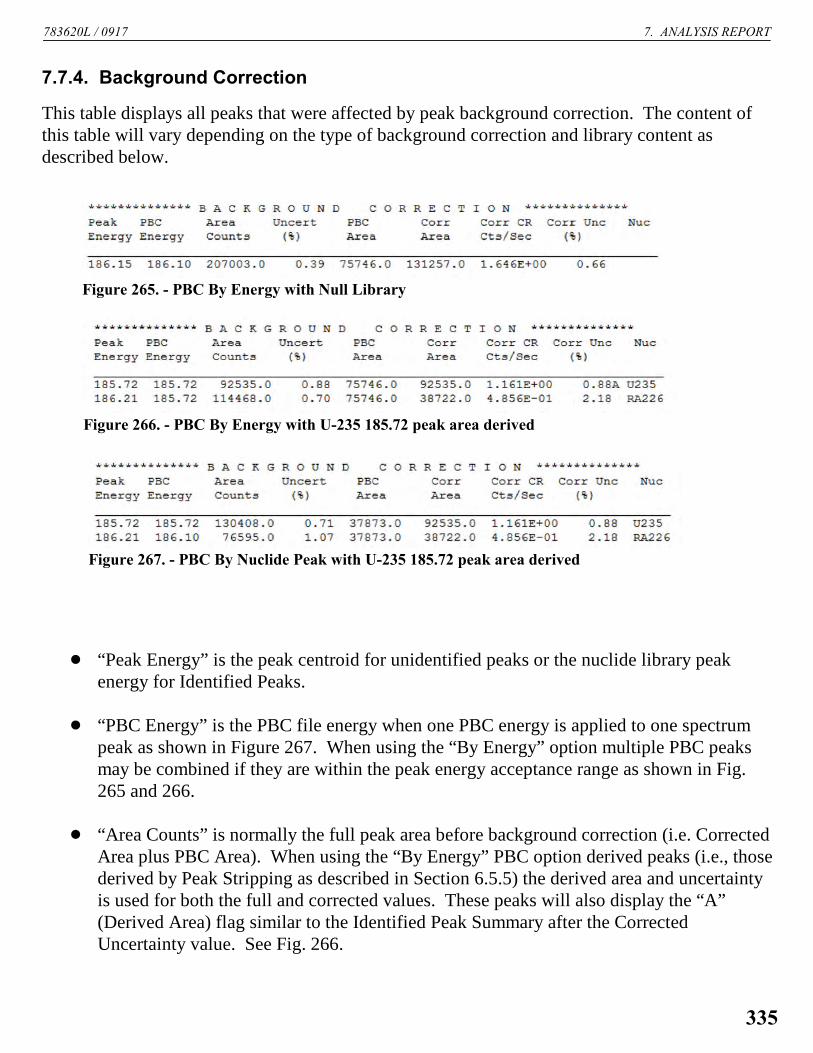
783620L / 0917 7. ANALYSIS REPORT
Figure 265. - PBC By Energy with Null Library
Figure 266. - PBC By Energy with U-235 185.72 peak area derived
Figure 267. - PBC By Nuclide Peak with U-235 185.72 peak area derived
7.7.4. Background Correction
This table displays all peaks that were affected by peak background correction. The content ofthis table will vary depending on the type of background correction and library content asdescribed below.
! “Peak Energy” is the peak centroid for unidentified peaks or the nuclide library peakenergy for Identified Peaks.
! “PBC Energy” is the PBC file energy when one PBC energy is applied to one spectrumpeak as shown in Figure 267. When using the “By Energy” option multiple PBC peaksmay be combined if they are within the peak energy acceptance range as shown in Fig.265 and 266.
! “Area Counts” is normally the full peak area before background correction (i.e. CorrectedArea plus PBC Area). When using the “By Energy” PBC option derived peaks (i.e., thosederived by Peak Stripping as described in Section 6.5.5) the derived area and uncertaintyis used for both the full and corrected values. These peaks will also display the “A”(Derived Area) flag similar to the Identified Peak Summary after the CorrectedUncertainty value. See Fig. 266.
335

GammaVision® V8 (A66-BW) 783620L / 0917
! “Uncert (%)” is the uncertainty of the full peak area and will usually be somewhat lowerthan the background corrected peak area. See exception noted previously for DerivedPeaks when PBC “By Energy” is enabled.
! “PBC Area” is the calculated area based on peak count rate in the PBC file and count timefor the sample. When using the “By Nuclide Peak Energy” PBC option the area isdetermined by the corresponding nuclide peak energy from the PBC table. When usingthe “By Energy” PBC option the area is the sum of all PBC peaks associated with thespectrum peak as described in Section 6.10.4.
! “Corr Area” is the peak area after background correction, or the derived peak area if PeakStripping was implemented as described in Section 6.5.5.
! “Corr CR cts/sec” is the “Corr Area” divided by Live Time.
! “Corr Unc (%)” is the uncertainty of the background corrected peak area. When using the“By Energy” background correction option, peaks with corrected uncertainty greater thanthe Peak Cutoff do not pass the peak acceptance test and would not be used in theremainder of the analysis process.
! “Nuc” is the nuclide name for Identified Peaks. Unidentified Peaks that have backgroundcorrection applied will be displayed as shown in Figure 265 when using the “By Energy”background correction option.
! Figures 265 and 266 are examples of PBC “By Energy” as compared to Figure 267 whichuses the PBC “By Nuclide Peak”. Both of the PBC peaks shown in Figure 267 arecombined as one background correction in Figures 265 and 266 because the energies fallwithin the “By Energy” acceptance range for this analysis.
! Figures 266 and 267 represent the same analysis with PBC “By Energy” and “By NuclidePeak” respectively. The corrected peak areas and uncertainties are the same in both cases,but the uncorrected peak area and uncertainty, and PBC area are different because of howthe background correction is applied with each method.
336

783620L / 0917 7. ANALYSIS REPORT
Figure 268.
7.7.5. Summary of Peaks in Range (ENV32 and NPP32 Only)
This table (Fig. 268) displays all of the peaks that were found during the analysis process with theclarifications below.
! The Library peak list option must be enabled on the Report tab for this table to bedisplayed.
! The peak data and nuclide activity are based a peak search run with no library peaks (i.e.,a Mariscotti peak search) and no peak stripping (interference correction) applied. Anypeaks identified using the Library Directed Peak Search that do not overlap those foundusing the Mariscotti search are also included in this table.
! The “Uncert” (uncertainty) value is 1-sigma counting uncertainty, which is directlycomparable to the Peak Cutoff acceptance criterion. Only peaks with1-sigma countinguncertainty below the Peak Cutoff value are reported.
! The “Corrctn Factor” (correction factor) is the effective efficiency at the specified energyand takes into account any geometry or attenuation corrections enabled.
! The nuclide names (“Nuc”) have all non-alphanumeric characters removed for tableformatting.
! All nuclides that have a photon energy within the Match Width × Calibration FWHM of alisted peak are listed as a possible source candidate along with the peak energy, branchingratio, calculated activity, and nuclide name. The specific activity for each potential nuclidecandidate is calculated under the assumption that the full peak area was generated entirelyby that nuclide such that all applicable correction factors (decay, efficiency, branchingratio, sample size, etc.) are applied except for any potential peak interferences. Thenuclide activity values from this table may be substituted for nuclide activity reported in
337

GammaVision® V8 (A66-BW) 783620L / 0917
Figure 269.
the Summary of Nuclides in Sample if it is determined that the peak was misidentified ormisinterpreted due to peak interferences. This type of correction may be desired in somecases for manual interference calculations, reporting of conservative activity results, or tocorrect for inaccurate nuclide identification. The data from this table can also be used tocompare the results of the Mariscotti vs Library Directed Peak Search and fitting to helpidentify where library or analysis option changes may be needed.
7.7.6. Unidentified Peak Summary
This table (Fig. 269) displays peaks found in the spectrum that were not associated with a librarynuclide, with the clarifications below.
! The Unknown peaks option must be enabled on the Report tab for this table to bedisplayed.
! Only peaks with1-sigma counting uncertainty below the Peak Cutoff value are reported.
! The uncertainty displayed is based on the Confidence level selected on the Report tab.
! The “Suspected Nuclide” is determined by selecting the nuclide from the suspect librarythat has the closest peak energy to the unidentified peak energy and is within theb30winds.ini (n30winds.ini for NAI32) file “Range Multiplier” parameter multiplied bythe peak FWHM. The Range Multiplier is normally set to 2.0 but you can modify this. Ifthere are no nuclides with peak energies in the specified range, the “Unknown Suspect”text from the b30winds.ini (n30winds.ini for NAI32) file is displayed in this column.
! If the b30winds.ini (n30winds.ini for NAI32) parameter “Unidentified Peak Summary andLibrary Peak Usage Format flag” is set to “T” (true), then the fifth column is labeled
338

783620L / 0917 7. ANALYSIS REPORT
Figure 270.
Figure 271.
“Efficiency * Area” and displays the Net Area divided by the effective efficiency (whichincludes any Geometry or Attenuation corrections). If this parameter is set to “F”, then thefifth column is labeled “Intensity Cts/Sec” and displays the net count rate as shown inFig. 270.
! The designators for peaks flags (Deconvolution, Shape, and Multiplets as applicable) canbe modified in the b30winds.ini (n30winds.ini for NAI32) file.
! The L, C, and M flags are applicable only to the NPP32 and ENV32 analysis engines.
7.7.7. Identified Peak Summary
This table (Fig. 271) displays peaks that were found in the spectrum and associated with a librarynuclide, with the clarifications below.
! The Library peak list option must be enabled on the Report tab for this table to bedisplayed.
! If the library is not found or the spectrum is not calibrated, this table is suppressed.
! If Manual Library Based Peak Stripping is enabled on the Analysis tab (WAN32 only),a separate table for peak data associated with each library is reported with the library namedisplayed at the beginning of the table.
339

GammaVision® V8 (A66-BW) 783620L / 0917
Figure 272.
! The designators for Deconvolution, Shape, and Derived Area (as applicable) can bemodified in the b30winds.ini (n30winds.ini for NAI32) file.
! If the b30winds.ini (n30winds.ini for NAI32) parameter “Zero Area Identified Peak flag”is set to “F” (false), then only peaks with 1-sigma counting uncertainty below the PeakCutoff and those resulting from Directed Fit (when enabled on the Analysis tab) areincluded in this table. If this parameter is set to “T” (true), additional peaks that did notpass the Peak Cutoff may be included in the list based on the analysis engine as follows:
— WAN32 and ROI32: Peak data are displayed for all peaks in the library.
— GAM32: Peak data are displayed for all peaks reported, but all library peaks may notbe reported depending on peak quality, library content, and analysis settings.
— NPP32: Deconvoluted peaks that are rejected may not be included in the peak list.Only the peak background and FWHM are displayed for peaks that do not meet thepeak cutoff criteria.
— ENV32 and NAI32: Some rejected peaks may be included in the list, but peak dataare not available.
7.7.8. Summary of Library Peak Usage
This table (Fig. 272) displays peaks that were found in the spectrum and associated with a librarynuclide with the clarifications below.
! The Library peak matrix option must be enabled on the Report tab for this table to bedisplayed.
! If the library is not found or the spectrum is not calibrated, this table is suppressed.
340

783620L / 0917 7. ANALYSIS REPORT
! If Manual Library Based Peak Stripping is enabled on the Analysis tab, a separate tablefor data associated with each library is reported with the library name displayed at thebeginning of the table.
! The table format and content are based on the analysis engine as follows:
— NPP32, ENV32, and NAI32:
P Average Nuclide Activity and Peak Activity values have corrections appliedincluding the activity scaling factor (based on the Multiplier, Divisor, and sampleSize entered on the System tab) and decay.
P The column to the right of the Peak MDA is the peak 1-sigma counting uncertaintyin percent.
P The first nuclide peak is one line below the applicable nuclide data.
P If the b30winds.ini (n30winds.ini for NAI32) “Zero Activity Isotope flag” flag isset to “T” (true), rejected nuclides and associated peaks are included in the table.The activity values are set to zero, but peak flags, MDA, and counting uncertaintyare displayed (as well as branching ratio and half-life if applicable based on the“Unidentified Peak Summary and Library Peak Usage Format flag” flag setting).Uncertainty values may be set to a default value of zero (NPP32) or 1E+03(ENV32) for peaks that are rejected. This may be due to the nuclide being rejectedprior to the Library Directed Fit process, the inability to physically fit a peak in thespectrum, or other peak rejection criteria. If this parameter is set to “F” (false),rejected nuclides are not displayed in this table.
P If Directed Fit is enabled on the Analysis tab, peak fit data associated withDirected Fit are displayed in this table. When using ENV32, all nuclides should bereported with an activity value. When using NPP32, nuclides that fail the Key Lineor Fraction Limit tests, or have interferences at key peaks, can still be reported withzero activity.
P Peak energies are listed in the library order regardless of the b30winds.ini
(n30winds.ini for NAI32) parameter “Sort Nuclide Peaks by Energy flag” setting.
P If the b30winds.ini (n30winds.ini for NAI32) parameter “Zero Area Library Peakflag” is set to “T” (true), display all nuclide library peaks even if they did not passthe analysis settings criteria. If this flag is set to “F” (false), only the peaks thatpassed the analysis settings criteria will be displayed, and a message summarizing
341

GammaVision® V8 (A66-BW) 783620L / 0917
Figure 273.
how many of the library peaks were found will be displayed below the nuclide peaklist (i.e., X of Y peaks found).
— WAN32, GAM32, and ROI32:
P Average Nuclide Activity is reported as Time of Count Total Activity in either ìCior Bq as selected on the System tab. This value has all corrections applied exceptfor activity scaling factor (based on the Multiplier, Divisor, and sample Sizeentered on the System tab) and decay.
P Peak Activity is reported as Time of Count Total Activity in either ìCi or Bq asselected on the System tab. This value has all corrections applied except for activityscaling factor (Multiplier, Divisor, and sample Size), decay, and RandomSumming.
P Peak uncertainty is not reported.
P The first nuclide peak is on the same line as the nuclide data as shown in Fig. 273.
P All nuclides are reported even when they are not identified (i.e., zero activity)regardless of the b30winds.ini (n30winds.ini for NAI32) “Zero Activity Isotopeflag” parameter setting.
P If Directed Fit is enabled on the Analysis tab, peak fit data associated withDirected Fit are displayed in this table. When using WAN32, nuclides that fail theKey Line or Fraction Limit tests, or have interferences at key peaks, can still bereported with zero activity.
P If the b30winds.ini (n30winds.ini for NAI32) “Sort Nuclide Peaks by Energy flag”flag is set to “T” (true), then nuclide peaks are listed in order of energy. If thisparameter is set to “F” (false), then nuclide peaks are listed in the library order.
342

783620L / 0917 7. ANALYSIS REPORT
P All nuclide library peaks are displayed regardless of the b30winds.ini (n30winds.ini
for NAI32) “Zero Area Library Peak flag” setting.
— All analysis engines:
P If the b30winds.ini (n30winds.ini for NAI32) “Unidentified Peak Summary andLibrary Peak Usage Format flag” parameter is set to “T” (true), the nuclide half-life(in days) is displayed under the COMMENTS header on the same line as thenuclide data, and the peak branching ratios are displayed in the right-most columnbefore the peak flags. If this parameter is set to “F”, the nuclide half-life andbranching ratios are omitted.
P If the b30winds.ini (n30winds.ini for NAI32) “Use Internal TCC Library Peaks”parameter is set to “T” (true), the nuclide peaks in this table (and throughout theanalysis process) will be based on the internal TCC library including the peak listand peak order which may (and likely will) differ from the original analysis library.Additionally, any peak flags set in the library are discarded. This configuration maynot generate optimal results for some applications. If this parameter is set to “F”,the peak list, peak order, and peak flags from the original library are used foranalysis. Only the Branching Ratio is adjusted for the coincidence summingcorrection. This configuration allows for improved optimization of the analysisresults.
! The legend of Nuclide Codes shown after the nuclide name, Peak Codes shown at the farright, and Peak Flags shown after the Peak Activity are reported after this table. These areexplained in the following section.
7.7.8.1. Summary of Library Peak Usage Flags
This table (Fig. 274) is displayed after the Summary of ROI Peak Usage and Summary of LibraryPeak Usage sections of the report. The Nuclide and Peak Codes listed at the bottom of the tableare based on flags set in the analysis library. The Peak Flags are defined as follows:
( This peak was used in the average nuclide activity calculation (even if any other sym-bols are displayed). For more information on the Weighted Average Nuclide Activity,see Section 6.7.1.
* The peak FW10M and FW25M were wider than the calibrated shape by more than 20%which would indicate that this might be a multiplet. However, deconvolution was notpossible because only one peak was in the library.
343

GammaVision® V8 (A66-BW) 783620L / 0917
Figure 274.
! This peak was in an area that was deconvoluted and the area of this component was zeroor negative. The peak was then removed as a component and the deconvolution redone.This usually indicates the peak was not present or the energy calibration needsadjustment.
? The peak FW25M is less than 80% of the calibration FW25M. This usually indicatesthat the peak has poor shape.
@ The peak FW25M was wider than the calibrated shape by more than 20%, but theFWHM was within 20% of the calibrated FWHM. This indicates there might be a smallpeak near the main peak that may need to be included in the library.
% The 1-sigma counting error was greater than the Peak Cutoff value set on the Analysistab.
$ This peak was identified as belonging to this nuclide, but the first non-interfered peakfor this nuclide was not identified or was disqualified. This may indicate that this peakwas not generated by the respective nuclide.
344

783620L / 0917 7. ANALYSIS REPORT
+ The abundance for this peak was higher than the running average of those included atthis point. For more information on the Weighted Average Nuclide Activity, seeSection 6.7.1.
- The abundance for this peak was lower than the running average of those included atthis point. For more information on the Weighted Average Nuclide Activity, seeSection 6.7.1.
= This peak was outside the user-specified limits for the analysis.
& When the library-directed centroid was recalculated after background subtraction, thecentroid value was outside the energy limits such that the peak could not be attributed tothis nuclide. This may occur with very small peaks where the peak shape is not welldefined, when the energy calibration needs adjustment, or if the library peak energiesneed to be corrected.
} The peak area for this peak was derived using other peaks for this nuclide. This isenabled by the library-based peak stripping option.
P Peak Background Subtraction was applied to this peak. (See Section 6.10.4 for detailson peak background subtraction.)
7.7.9. Discarded Isotope Peaks
This table (Fig. 275) displays peaks associated with a nuclide that was rejected during theanalysis due to a failed Key Line or Fraction limit test, with the clarifications below.
! Isotopes may be discarded when using WAN32, ROI32, and NPP32 analysis enginesbecause the rejection criteria are evaluated after the Library Directed Peak Search hasassociated peaks with a nuclide. For GAM32 and ENV32 analysis engines, this tableshould be empty because the Key Line and Fraction Limit tests are implemented duringthe Library Reduction step at the beginning of the analysis process before the LibraryDirected Peak search, which assigns nuclide peaks.
! If the b30winds.ini (n30winds.ini for NAI32) parameter “Print Discarded Peak Table flag”is set to “T” (true), this table is displayed for all analysis engines except for GAM32. Ifthis parameter is set to “F” (false), this table is suppressed.
345

GammaVision® V8 (A66-BW) 783620L / 0917
Figure 275.
Figure 276.
7.7.10. Summary of Discarded Peaks
This table (Fig. 276) displays peaks that were evaluated during the Library Directed Peak Searchand rejected from use in calculating Nuclide Activity, with the following notes:
! A peak may be rejected due to failing a peak test, rejection of the nuclide due to key lineor fraction limit tests, peak activity outside the uncertainty range for the nuclide averageactivity, as well as other factors.
! This table is displayed only when the Library peak matrix option is disabled on theReport tab.
! See Section 7.7.8.1 for peak flag descriptions.
346

783620L / 0917 7. ANALYSIS REPORT
Figure 277.
7.7.11. Summary of Nuclides in Sample
This table (Fig. 277) displays the final nuclide activity results with the clarifications below.
! The Nuclide abundance option must be enabled on the Report tab for this table to bedisplayed.
! If the library is not found or the spectrum is not calibrated, this table is suppressed.
! Nuclide Activity Notes:
— The “Time of Count” Activity column is weighted by the peak branching ratios asdescribed in Section 6.10.2, and includes all corrections except for decay duringcollection and decay to collection time. Note that this includes Decay DuringAcquisition, which is set on the Decay tab.
— The “Time Corrected Activity” column is weighted by the peak branching ratios asdescribed in Section 6.10.3, and has all corrections applied including decay. It is onlydisplayed in this table when Decay During Collection or Decay to Collection Time isenabled on the Decay tab.
347

GammaVision® V8 (A66-BW) 783620L / 0917
! Uncertainty Notes:
— Uncertainty Counting and Total Uncertainty data are reported in either percent oractivity units as specified on the Report tab.
— The Total Uncertainty column is only displayed if the Total Uncertainty option isspecified on the Report tab.
— If activity is set to zero, which may occur when using Directed Fit, the default percentuncertainty is 1000%.
— Uncertainty is omitted, or set to zero for some analysis engines, if the nuclide activityis reported with the “<“ flag (i.e., less than the calculated MDA value.)
! MDA Notes:
— Nuclides that have the “No MDA Calculation” flag set in the library will not calculatean MDA value. If an activity value is not calculated, these nuclides will be omittedfrom this table.
— When a nuclide is reported with the “<“ flag, the MDA values are displayed in theTime of Count and Time Corrected Activity columns as applicable.
— For all analysis engines except for GAM32, if the b30winds.ini (n30winds.ini forNAI32) parameter “Print MDA flag” is set to “T” (true), the MDA value is reported inthe far right column for nuclides that have an activity value calculated. If thisparameter is set to “F” (false), nuclide MDA is not reported for nuclides that have anactivity value calculated. The GAM32 analysis engine does not report MDA valueswhen nuclide activity is calculated regardless of this flag setting.
— The MDA Column header is determined by the b30winds.ini (n30winds.ini for NAI32)parameter “Nuclide Summary MDA Header,” which is set to “MDA” by default.
! Total Activity and Total Decayed Activity at the bottom of the table are the sum of therespective nuclide activity columns except that nuclides marked with the following flagsare not included in the totals: *, &, <, B, F, (H for Decay Activity only).
! Some nuclide flags may not be reported if no nuclides in the list meet the specifiedcriteria. Nuclide flags are defined as follows:
348

783620L / 0917 7. ANALYSIS REPORT
# - All peaks for the activity calculation had bad shape. This does not invalidate thenuclide activity, but may indicate that the peaks may have interference, few counts(as may also be accompanied with high uncertainty), tails due to detector perform-ance, or other anomalies that may warrant investigation.
* - This nuclide activity was omitted from the total activity because the “Activity Notin Total” flag was set for this nuclide in the library.
& - This nuclide activity was omitted from the total activity because the “Activity Notin Total” flag was set for this nuclide in the library, and all of the peaks had badshape. This flag is a combination of the # and * flag conditions.
< - The nuclide MDA is reported in the Time of Count and Decay Corrected activitycolumns as applicable.
A - The nuclide activity is lower than the calculated MDA value. This condition doesnot necessarily mean that the nuclide activity is invalid or that the true activity mustbe below the detection limit. This condition may be due to a liberal peakacceptance criterion (i.e., Peak Cutoff), using Directed Fit in the analysis optionsfor nuclides with no substantial peaks, or when nuclide activity is near the detectionlevel depending on the MDA method specified on the System tab. Furtherinvestigation may be warranted for this condition.
B - This flag is a combination of the “A” and “F” flags. Activity is less than the calcu-lated MDA, and the Key Line or Fraction limit test failed.
C - The nuclide activity is lower than the Critical Level MDA method, which isbased on the MDA Method 2 described in Section 6.9.2.2. This condition may bedue to a liberal peak acceptance criteria (i.e., Peak Cutoff), or when usingDirected Fit in the analysis options for nuclides with no substantial peaks. Furtherinvestigation may be warranted for this condition.
F - The Fraction Limit or Key Line test failed for this nuclide. Normally, nuclides thatfail one of these tests would be reported as <MDA, but some conditions (i.e.,Directed Fit or when using the WAN32 analysis engine) may result in nuclideactivity being reported.
H - The number of half-lives specified in the b30winds.ini (n30winds.ini for NAI32)file for the “Half lives decay cutoff” parameter has been exceeded for this nuclide.If this occurs, the Time of Count Activity is reported as “>X Halflives” and theTime of Count Activity is reported based on the analysis engine as follows:
349

GammaVision® V8 (A66-BW) 783620L / 0917
Figure 278.
P WAN32, ROI32, ENV32, and NAI32: Time of Count activity is reported.
P GAM32: The “<“ flag and MDA value are reported.
P NPP32: Time of Count activity is omitted.
I - This flag is only applicable when the ISO NORM table is enabled on the Reporttab. It is displayed if the b30winds.ini (n30winds.ini for NAI32) parameter“Maximum ISO NORM MDA ratio factor” is exceeded. When this factor isexceeded, the ISO NORM Detection Limit (MDA) is also limited to a maximumvalue, as described in Section 6.17.2.1.
7.7.12. Summary of Nuclides (ISO-NORM)
This table (Fig. 278) displays the final ISO NORM compliant nuclide activity results, with theclarifications below.
! If the library is not found or the spectrum is not calibrated, this table is suppressed.
! If all peaks for a nuclide are outside of the analysis range, only the nuclide name and flags(if any) are reported.
! Each nuclide has two rows of data with the respective headers shown at the top of thetable.
350

783620L / 0917 7. ANALYSIS REPORT
! Activity is the same as the “Time of Count Activity” reported in the Summary of Nuclidesin Sample section.
! Corrected_Act is the same as the “Time Corrected Activity” reported in the Summary ofNuclides in Sample Section. This field is omitted and the remaining columns shifted to theleft if Decay During Collection and Decay to Collection are not enabled on the Decaytab. If either of these decay options are enabled, and the b30winds.ini (n30winds.ini forNAI32) parameter “Half lives decay cutoff” is exceeded, the message “>X Halflives” isdisplayed and none of the other nuclide data is included in this table.
! Counting_Unc is the same as the “Counting Uncertainty” reported in the Summary ofNuclides in Sample section.
! Total_Unc is the same as the “Total Uncertainty” reported in the Summary of Nuclides inSample section. This field is omitted and the remaining columns shifted to the left if TotalUncertainty is not enabled on the Report tab.
! Det_Limit is calculated per Section 6.17.2.2 for MDA Method 19, “ISO 11929 DetectionLimit (MDA),” even if a different MDA method is specified on the System tab for report-ing in all other sections of the report.
! Act_Best (Activity based on best estimate of peak area [Ah]) is calculated perSection 6.17.3.3.
! Act_Low (Lower Limit of peak area [A<]) is calculated per Section 6.17.3.7.
! Act_High (Upper Limit of peak area [A>]) is calculated per Section 6.17.3.7.
! Det_Thres. (Critical Level or Decision Threshold [ACL]) is calculated per MDA Method18, “ISO Decision Threshold (CL)”; see Section 6.17.2.1.
! Unc_Best. (Uncertainty of the best estimate activity [óAh]) is calculated per MDA Method19, “ISO Detection Limit (MDA)”; see Section 6.17.2.2.
7.7.13. Iodine Equivalence and Average Energy Calculations
These parameters (Fig. 279) are displayed after the nuclide summary tables when the applicablecalculation is enabled on the Isotopes tab and the nuclide summary section of the report isenabled on the Report tab. Refer to Section 6.14 for details on Iodine Equivalence andSection 6.13 for details on Average Energy.
351

GammaVision® V8 (A66-BW) 783620L / 0917
Figure 279.
Figure 280.
7.7.14. DAC Calculations
This section (Fig. 280) is displayed after the nuclide summary tables when the calculation isenabled on the Isotopes tab. Refer to Section 6.15 for details on the DAC calculation.
7.8. The EDF Special Application Report
The EDF Special Application Report (see Section 5.5.1.9) is appended to the end of the standardGammaVision report. This table lists the Gamma Total settings used in the analysis, and thequantitative results.
Figures 281 and 282 shows representative Gamma Total background and Gamma Total Reportinganalyses.
352

783620L / 0917 7. ANALYSIS REPORT
Figure 281. Gamma Total Background Report.
Figure 282. Gamma Total Report.
353

GammaVision® V8 (A66-BW) 783620L / 0917
[Intentionally blank]
354

8. QUALITY ASSURANCE
8.1. Introduction
The accuracy and reproducibility of results of a data acquisition system should be verified on aperiodic basis. Quality Assurance (QA) in GammaVision supplies a means for doing this inaccordance with ANSI N13.30 and N42.14. The detector-shield background, detector efficiency,peak shape, and peak drift can be tracked with warning and acceptance limits. The latter use acheck source. These results are stored in a database and can be displayed and charted. The data-base can be accessed with commercially available database products, including Microsoft Access.The information stored in the database for each detector includes:
! Total Background — The count rate (counts/sec), over the entire spectrum, of the environ-mental background (that is, with no source present).
! Total Activity — The sum of the decay-corrected activities of the nuclides measured in thesource, as defined in the analysis library.
where:N = the number of nuclides in the analysis libraryDC = the decay correction factor for nuclide x in the analysis libraryA = the calculated activity, in becquerels, for nuclide x in the analysis library
! Average FWHM Ratio — The sum of the ratio of each peak’s measured FWHM vs. itscalibrated FWHM, divided by the total number of peaks, for all peaks defined in the analysislibrary.
CAUTION Running the MCB Configuration program can affect the continuity of your QAmeasurements in GammaVision. Be sure to read Section 2.4!
355

GammaVision® V8 (A66-BW) 783620L / 0917
where:P = the number of identified peaks in the spectrumFWHMMeas = the measured FWHM of analysis library peak x, in keVFWHMCal = the calibrated FWHM of analysis library peak x, in keV
! Average FWTM ratio — The sum of the ratio of each peak’s measured FWTM vs. itseffective calibrated FWTM, divided by the total number of peaks, for all peaks defined in theanalysis library.
where:P = the number of identified peaks in the spectrumFWHMMeas = the measured FWTM of analysis library peak x, in keVFWHMEffCal = the effective calibrated FWTM of analysis library peak x, in keV
! Average Library Peak Energy Shift — The average of the deviation of the measured peakenegy from the expected peak energy, for all energies defined in the analysis library.
where:E = the number of identified peak energies in the spectrumEMeas = the measured peak energy corresponding to analysis library energy x, in keVELib = the expected peak energy x from the analysis library, in keV
The background should be monitored to verify that the detector and shield have not been contam-inated by radioactive materials. The value stored is the total count rate which is independent ofthe count time and any specific isotopic contamination. A background analysis report can beprinted after the analysis completes.
The total activity of a calibration or check source will check the efficiency calibration currently inuse and the general operating parameters of the system, including source positioning, contami-nation, library values, and energy calibration. This activity calculation uses the general analysisprogram to ensure that the total system is checked.
356

783620L / 0917 8. QUALITY ASSURANCE
Figure 283. QASubmenu.
NOTE Use nuclides with long half-lives for your QA measurements. Short-lived nuclides willdevelop poor peak shapes as they decay.
ORTEC Application Note 55 contains more information and help on starting and running QA forgamma spectroscopy.
The FWHM and FWTM values will check the electronic noise and pole-zero adjustment of theamplifier. The peak shift checks to verify that the system gain and zero offset have not changed.
8.1.1. Using QA Results to Diagnose System Problems
A gradual deterioration of the FWHMMeas/FWHMCal ratio usually means the detector leakagecurrent has increased.
A sudden deterioration of the FWHMMeas/FWHMCal ratio suggest that additional noise has beenintroduced into the system. Commonly, this can arise from:
! A noisy motor introduced into the ac line! RF interference! Electronic failure of a component in the detector, preamplifier, or MCB
Generally, these problems will also cause the FW.1M ratio check to fail.
If the FW.1M ratios fail but the FWHM ratios are acceptable, this could indicate:
! Incorrect pole zero! Neutron or other radiation damage to the detector
8.2. QA Submenu
Figure 283 shows the QA submenu under the Acquire menu. Thesecommands allow you to accomplish the three major QA functions inGammaVision:
The three parts of QA in GammaVision are:
1) Establishing and entering the settings, or “ground rules,” for QA.
2) Measuring background and sample. You perform this periodically,and it is automatically logged into a database by the program.
357

GammaVision® V8 (A66-BW) 783620L / 0917
3) Analyzing the QA database and generating reports. This includes GammaVision’s Status andControl Chart features, which allow you to view the current status of measurements for theDetector and/or view and print the data stored in the database as a control-chart display.
8.2.1. Settings...
The QA settings include the upper and lower radionuclide activity limits which, when exceeded,indicate that the system is not operating correctly. There are two levels of limits. The warninglimits are determined by the settings in the Low and High fields in the Quality Assurance Set-tings dialog in Fig. 284. The alarm limits those outside of the Minimum and Maximum fields. Ifthe result of a QA measurement is outside the warning limits, a warning dialog is displayed. If theQA result is outside the alarm limits, a violation dialog is displayed. Moreover, if the LockAcquire on Violation(s) box is marked, the violation must be corrected and the QA measurementrepeated before the out-of-limits Detector can be used to collect more data.
Generally, after setup, these levels should not be changed without careful consideration.
NOTE If the “Unable to Access QA Database” message is displayed when you issue theSettings... command, the QA database file GvQa32.Mdb is not currently located in thefolder in which it was originally created (i.e., it has been moved, renamed, or deleted).See Section 8.4.
8.2.1.1. Establishing QA Settings
Click Settings... to open the Quality Assurance Settings dialog shown in Fig. 284. This dialogcontains three main data-entry areas:
! BACKGROUND Acquisition time and Count Rate Limits! SAMPLE Type Analysis Settings File! SAMPLE Analysis Parameter Limits
Several preliminary steps must be taken to determine the QA settings:
1) Backgrounds must be counted to determine reasonable levels.
2) Samples must be counted for total activity to obtain expected values, since total activity isdetector and QA source dependent.
3) A QA library containing only the nuclides in the QA source must be created using the nuclidelibrary editor (see Section 5.6).
358

783620L / 0917 8. QUALITY ASSURANCE
Figure 284. QA Settings Dialog.
4) A sample type settings file (.SDF) must be created which contains the defaults for the QAacquisition and analysis (see Section 5.5.1.1).
5) A QA database file must exist. The GammaVision QA database, GvQa32.Mdb, is installed aspart of the standard GammaVision installation, and should be located in the \User directory onthe drive where GammaVision was installed. However, if you select the Settings... commandand GammaVision cannot find GvQa32.Mdb (or if the database file cannot be used for somereason), a warning message will ask if you wish to create a QA database. Click OK to startthe QA database setup wizard and go to Section 8.4 for instructions. When the database hasbeen successfully created, you will be automatically returned to the Quality AssuranceSettings dialog.
All the information gathered in preliminary Steps 1–4 can be entered in the Quality AssuranceSettings dialog.
The BACKGROUND Acquisition time and Count Rate Limits are entered using the informa-tion gathered in Step 1 above. Enter the Real time or Live time in seconds; for backgroundspectra, the dead time is near zero, so these are usually equal.
359
GammaVision® V8 (A66-BW) 783620L / 0917
The Minimum and Maximum count-rate limits are the acceptance thresholds for the alarm limit.Acceptance thresholds are used to indicate that the system is operating far from the expectedconditions, and can be used to prevent data acquisition from being performed at all until thecondition is corrected. If the Lock Acquire on Violation(s) box is marked and an acceptancethreshold is exceeded, the Detector is automatically locked out from use until the problem iscorrected and QA is rerun. The Low and High count-rate limits are the warning limits, andexceeding them will cause warning messages to be displayed.
The Background Report is printed after the analysis if you mark the Create Background Reportcheckbox. The report can either be saved to disk or printed.
The SAMPLE Type Analysis Settings File is the .SDF file created for QA in Step 4 usingAnalyze/Settings/Sample Type.... Click Browse... to select the .SDF file. To edit the .SDF file,click Edit.... This will open the Analysis Options dialog (see Section 5.5.1.1). Especially relevantsample type settings include:
! Sample type description! Acquisition presets! QA nuclide library file (the one created in Step 3)
If you wish to save or print a SAMPLE Report after the analysis, mark the Create SAMPLEReport box.
On the left of the SAMPLE Analysis Parameter Limits section are checkboxes for marking thelimits to be tracked. Total Activity (Bq), Average Peak Shift (keV), Average FWHM Ratios,and Average FWTM Ratios are the choices. Mark the limits to be tracked. The first timeGammaVision QA is set up, click the Suggest button (on the right) to enter factory-set limits.After this, use the Suggest button with caution, because clicking on it again will reset all thelimits to the previously defined settings. The actual limits can be determined from the samplescounted in Step 2 above.
Click OK. GammaVision will check the measurement limits to determine if they are set consis-tently. If they are, the dialog will close; if not, a message will be displayed on the Marker Inform-ation Line and the dialog will remain open so the limits can be changed. QA data can now becollected using Acquire/QA/Measure Background and Acquire/QA/Measure Sample.
360

783620L / 0917 8. QUALITY ASSURANCE
Figure 285. Begin Background QACount.
Figure 286. Background WarningMessage.
Figure 287. Starting Sample Type QAMeasurement.
8.2.2. Measure Background
This command opens the dialog in Fig. 285, toverify that all sources have been removed fromthe Detector before proceeding. Confirm thatall sources have been removed for a backgroundmeasurement, click OK–Start. The remainingfunctions are performed automatically.
Mark the Overwrite (repeat) previousbackground measurement checkbox (byclicking on it) if the previous measurement was in error. If a sample QA has been run since thebackground QA, the previous background run cannot be overwritten. For example, if a problemwas detected, fixed, and this run is to verify the repairs, check the box so the “bad” value is notkept in the database. Click OK.
If the background is outside the set limits, a warningsimilar to Fig. 286 is displayed.
8.2.3. Measure Sample
This command opens the Sample QA Measurementdialog (Fig. 287). It is a reminder to place the QAsource on the Detector. Click Overwrite to replacethe last measurement. Click OK–Start to begin thecount.
The QA source spectra are collected forthe preset time and analyzed automatically.The analysis results are compared with thelimits. If the result is outside the limits, awarning is displayed. The results are also stored inthe QA database.
361

GammaVision® V8 (A66-BW) 783620L / 0917
Figure 288. Showing Status of QA Measurements for a Detector.
Figure 289. Control Chart Example.
8.2.4. Status...
The QA status for the currently selected Detector is displayed as shown in Fig. 288. Click OK toclose the dialog.
8.2.5. Control Charts...
The Control Chart... functions display thedata stored in the QA database as a controlchart. The displayed data can be scrolledbackward or forward across the screen sothat all collected data can be viewed. Atypical chart is shown in Fig. 289. Theshort dashed lines represent the warninglimits and the long dashed lines representthe acceptance threshold limits. Note thatif you call this command before any QAsettings are established in theGammaVision QA database, you willreceive an error message. Acknowledgethe message and set up your detectors inthe QA database.
362

783620L / 0917 8. QUALITY ASSURANCE
Figure 290. QA ChartFile Menu.
Figure 291. Scale Menu.
Figure 292. Plot VariableMenu.
Figure 293. Detector Pick List.
Figure 290 shows the control chart File menu, which contains the Print Graph command forprinting the current graph on the current printer; a standard Windows Print Setup... commandfor selecting the printer and its setup features, such as landscape vs. portrait layout, paper size,number of copies, and device control options; the Exit command for closing the QA ChartProgram (this duplicates the dialog’s upper-right Close box); and an About box providingversion information about the chart program.
Choose the chart time period (Week, Month, or Quarter) from the Scale menu (Fig. 291).
The Plot Variable menu (Fig. 292) contains functions for selecting Activity, Peak Energy, PeakWidth @ Half Max, Peak Width @ Tenth Max, or Background.
The Detector menu item opens the list of Detectorsfor which background and sample measurementshave been made (Fig. 293). Select a Detector forthis control chart and click OK.
Offline processing of the QA data-base (includingdetailed trend analyses) can be done outside ofGammaVision. The database format used is well-documented and compatible with a number ofpopular software products including MicrosoftAccess.
NOTE We strongly recommend that you backup any GammaVision database filesbefore performing manipulations onthem outside of GammaVision.
363

GammaVision® V8 (A66-BW) 783620L / 0917
Figure 294. QAChart File Menu.
The Options menu (Fig. 294) includes an Always On Top com-mand, which keeps the QA window on top of all other windows,no matter which window (in GammaVision or any other program)might be active.
The Fixed Vertical Scale command adds flexibility in displayingcontrol charts both onscreen and on printouts, for comparison withother charts.
! Fixed Vertical Scale Off (no check mark) — In this mode, the vertical scale of the graph isadjusted so that all points are shown to scale. All points are black. If one or more data pointsare substantially out of range, the graph may be quite compressed vertically.
! Fixed Vertical Scale On (check mark) — In this mode, the vertical scale of the graph is set toshow the upper and lower alarm limits as full scale. The data points within the alarm limits arecolored black. Out-of-range points are displayed in red at the lower or upper limits of thegraph, at the proper horizontal coordinate. The out-of-range points are printed as a questionmark ( ? ).
To switch between the two display modes, click the menu item to mark it with a checkmark orunmark it.
Figures 295 through 298 show the screen and printout for a QA data set with Fixed VerticalScale on, then off. Compare the location of the points that exceed alarm limits in Figs. 295and 296 to the location of the question marks in Figs. 297 and 298.
364

783620L / 0917 8. QUALITY ASSURANCE
Figure 295. Control Chart On Screen with Fixed Vertical ScaleOn.
Figure 296. Printout of Control Chart with Fixed Vertical ScaleOn.
365

GammaVision® V8 (A66-BW) 783620L / 0917
Figure 297. Control Chart On Screen with Fixed Vertical ScaleOff.
Figure 298. Printout of Control Chart with Fixed Vertical ScaleOff.
366

783620L / 0917 8. QUALITY ASSURANCE
8.3. Quality Assurance Example
This section discusses how to set up QA for a new detector in GammaVision, then performbackground and check-source measurements for the detector.
1) From the detector droplist on the toolbar, select the MCB that has the new detector. ThisMCB will now be displayed in the active spectrum window.
2) We will assume our check source was calibrated at 1.0 ìCi of 60Co activity and 2.0 ìCi of137Cs activity on June 27, 2000. The total expected activity measured today and decay-corrected back to the calibration date is 3.0 ìCi. We will count the source in the sameposition for 10 minutes each day to verify the detector efficiency and calibration have notchanged. It is unlikely the actual detector efficiency has changed, but the calibration filemight have changed or electronic noise might be interfering with the spectrum collection. Wewill count background for 120 seconds to verify the detector is not contaminated (if thedetector were contaminated with the same isotopes as in the QA source, the QA activitywould be incorrect) .
3) Use the GammaVision Library Editor on the Library menu to prepare a QA librarycontaining only 60Co and 137Cs, and save it the library as QA.lib.
4) Select Acquire/QA/Settings... to display the Quality Assurance Settings dialog for thisdetector (Fig. 299), then go to the SAMPLE Type Analysis Settings File section and clickthe Edit button. This will open the Analysis Options dialog (Fig. 300), which will allow us tocreate a sample defaults (.SDF) file for analyzing the QA acquisitions for this detector.
5) We will now enter the following analysis options for this .SDF file:
! On the Sample tab, click the Presets button to open the Presets dialog for this MCB type,then enter a Live Time preset of 600 seconds.
! In the Nuclide Library section, unmark the Internal box, then browse to retrieve thenewly created QA.lib file.
! Click the Decay tab. Mark the Collection checkbox and enter 06/27/2000 as the Date and12:00:00 as the Time. The format for the date and time will be determined by theWindows settings for the host computer.
! Return to the Sample tab, click Save As..., and save this file as QA.SDF.
367

GammaVision® V8 (A66-BW) 783620L / 0917
Figure 299. Example of Quality Assurance Settings.
Figure 300. Typical Settings for Quality Assurance Analysis.
368

783620L / 0917 8. QUALITY ASSURANCE
! Click OK to close the Analysis Options dialog. This will return you to the QualityAssurance Settings dialog.
6) In the BACKGROUND Acquisition section, enter a Live Time preset of 120 seconds. Enterarbitrary count-rate values for the Low and High background settings until you know whatthe realistic numbers should be. Do not use zero for the Low limit; if you do, you will notreceive a warning if the detector is not counting (for instance, if it is disconnected).Remember that these values are count rates, so are independent of the counting time.
7) Select the QA.SDF file in the SAMPLE Type Analysis Settings File section.
8) The expected value of the activity of the sample is 1.1E+5 Bq (3.0 ìCi). Scale this up anddown by 10% for Low/High and 20% for Minimum/Maximum into activity fields. Thesevalues are shown in the SAMPLE Analysis Parameter Limits section in Fig. 299.
You are now ready to collect data for the QA background followed by the QA check sourcemeasurements.
9) Select Acquire/QA/Measure Background... to start the background process. You will beprompted to remove all the sources from the detector and click OK-Start. The backgroundspectrum will be collected and summed, and stored in the QA database, GvQa32.Mdb. If anylimits were exceeded, a warning message will be displayed.
10) Select Acquire/QA/Measure Sample... to start the sample process. You will be prompted toplace the QA source in the proper place on the detector and click OK-Start. The samplespectrum will be collected and analyzed, and the results stored in the QA database. If anylimits were exceeded, a warning message will be displayed.
11) Note the Lock Acquire on Violation checkbox in the QA settings dialog. If this box ismarked and a limit is exceeded, GammaVision will display a QA warning each time you tryto use the detector until the QA problem is corrected.
12) The background and sample spectra will automatically be stored according to the QA FilePrefix and QA File Sequence number entered in Fig. 299.
You have now completed a QA setup and system verification, and have stored theresults in the QA database.
369
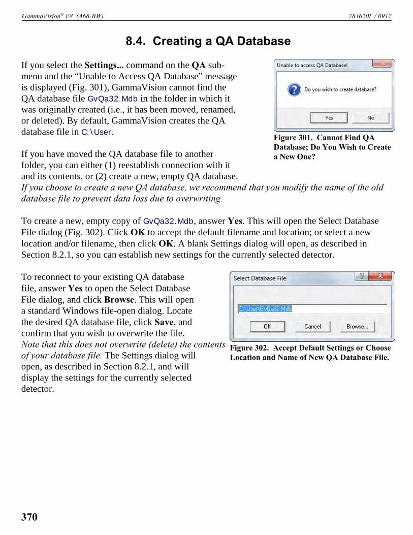
GammaVision® V8 (A66-BW) 783620L / 0917
Figure 301. Cannot Find QADatabase; Do You Wish to Createa New One?
Figure 302. Accept Default Settings or ChooseLocation and Name of New QA Database File.
8.4. Creating a QA Database
If you select the Settings... command on the QA sub-menu and the “Unable to Access QA Database” messageis displayed (Fig. 301), GammaVision cannot find theQA database file GvQa32.Mdb in the folder in which itwas originally created (i.e., it has been moved, renamed,or deleted). By default, GammaVision creates the QAdatabase file in C:\User.
If you have moved the QA database file to anotherfolder, you can either (1) reestablish connection with itand its contents, or (2) create a new, empty QA database.If you choose to create a new QA database, we recommend that you modify the name of the olddatabase file to prevent data loss due to overwriting.
To create a new, empty copy of GvQa32.Mdb, answer Yes. This will open the Select DatabaseFile dialog (Fig. 302). Click OK to accept the default filename and location; or select a newlocation and/or filename, then click OK. A blank Settings dialog will open, as described inSection 8.2.1, so you can establish new settings for the currently selected detector.
To reconnect to your existing QA databasefile, answer Yes to open the Select DatabaseFile dialog, and click Browse. This will opena standard Windows file-open dialog. Locatethe desired QA database file, click Save, andconfirm that you wish to overwrite the file.Note that this does not overwrite (delete) the contentsof your database file. The Settings dialog willopen, as described in Section 8.2.1, and willdisplay the settings for the currently selecteddetector.
370

9. KEYBOARD FUNCTIONS
This chapter describes the GammaVision accelerator keys. The keys described in this section aregrouped primarily according to location on the keyboard and secondarily by related function.
9.1. Introduction
Table 16 provides a quick reference to all of the GammaVision keyboard and keypad functions.These accelerators are also illustrated in Fig. 303, and discussed in more detail in the remainderof the chapter.
The accelerators are available only in the GammaVision window. The title bar must be high-lighted with the active title bar color (as set up in Windows Control Panel). In addition, the activecursor — or input focus — must be in one of the spectrum windows. Similar to other Windowsapplications, the focus can be switched between GammaVision and other applications by clickingon the Windows Taskbar, pressing <Alt + Tab>, or, if the inactive window is visible, pointingwith the mouse at some spot in the inactive window and clicking.
The multi-key functions, such as <Alt + 1> or <Shift + 6>, are executed by holding down thefirst key (e.g., <Alt>, <Shift>, or <Ctrl>) while pressing the key that follows the “+” sign in thebrackets, then releasing both keys simultaneously. Functions that use the keypad keys begin withthe word Keypad, e.g., Keypad<5>.
As usual for any Windows application, the menus are accessed by clicking on them with themouse, or by using the Alt key plus the key that matches the underlined letter in the menu itemname. For example, the multi-key combination to activate the File menu is <Alt + F>.
Note that the GammaVision accelerator keys do not interfere with Windows menu operations ortask switching. For example, when a menu is active (i.e., pulled down), the <7>/<6> and<8>/<9> keys revert to their normal Windows functions of moving across the menu bar andscrolling up/down within a menu, respectively. As soon as the menu is closed, they behave asGammaVision accelerators again.
9.2. Marker and Display Function Keys
9.2.1. Next Channel <6>/<7>
When not in rubber-rectangle mode, the right and left arrow keys move the marker by onedisplayed pixel in the corresponding direction. This might represent a jump of more than onespectral data memory channel, especially if the horizontal scale in channels is larger than thewidth in pixels of the window (see the discussion in Section 4.2).
371

GammaVision® V8 (A66-BW) 783620L / 0917
Key Function<9> or <F5> Change vertical scale so spectrum peaks appear smaller (vertical zoom out).<8> or <F6> Change vertical scale so spectrum peaks appear larger (vertical zoom in).<6> Move marker to higher channel. <7> Move marker to lower channel. <!> or <F7> Narrow the horizontal scale.<+> or <F8> Widen the horizontal scale.<Ctrl + 6> Jump to next higher peak.<Ctrl + 7> Jump to next lower peak.<Shift + 6> Jump to next higher ROI. In rubber rectangle mode, shift rectangle right (to higher energy/channel) one pixel.<Shift + 7> Jump to next lower ROI. In rubber rectangle mode, shift rectangle left (to lower energy/channel) one pixel.<Shift + 8> Shift the Compare spectrum up. In rubber rectangle mode, shift rectangle up (away from baseline) one pixel.<Shift + 9> Shift the Compare spectrum down. In rubber rectangle mode, shift rectangle down (toward baseline) one pixel.<Alt + 6> Advance to next library entry.<Alt + 7> Move back to previous library entry.<PageUp> Jump to higher channel number in 1/16th-screen-width increments.<PageDown> Jump to lower channel number in 1/16th-screen-width increments.<Home> Jump to first channel of the full spectrum.<End> Jump to last channel of the full spectrum.<Ctrl + Fi> Select Detector i (i = 1 to 12, in pick list order).<F2> Switch ROI bit control from OFF to SET to CLEAR.<F3> In MCBs with ZDT Mode, switch between the two spectra stored in ZDT mode.<Shift + F3> In Compare mode when comparing ZDT spectra, hold the initial spectrum in its current ZDT view (ERR or ZDT) and
toggle the Compare spectrum between its ZDT views.<F4> or <Alt + 6> Switch between displaying selected Detector and buffer.<F5> or <9> Change vertical scale so spectrum peaks appear smaller (vertical zoom out).<F6> or <8> Change vertical scale so spectrum peaks appear larger (vertical zoom in).<F7> or <!> Change the horizontal scale so peaks appear narrower (horizontal zoom out)<F8> or <+> Change the horizontal scale so peaks appear wider (horizontal zoom in)<Alt + F7> Reset both horizontal and vertical scaling to view complete spectrum.Keypad<!> Zoom out.Keypad<+> Zoom in.Keypad<5> Center expanded display on cursor.Keypad</> Switch between logarithmic and linear vertical scaling.Keypad<*> Switch to auto vertical scale.Insert<Ins> Mark the peak region around the cursor as an ROI.Delete<Del> Clear the ROI.<Alt + 1> Start acquisition in selected Detector.<Alt + 2> Stop acquisition in selected Detector.<Alt + 3> Clear data in selected Detector.<Alt + 5> Copy data in the selected Detector to the buffer.<Alt + 6> or <F4> Switch between displaying selected Detector and buffer.<Alt + !> Decrease amplifier fine gain by smallest increment (where supported).<Shift + Alt + !> Decrease amplifier fine gain by several increments.<Alt + +> Increase amplifier fine gain by smallest increment.<Shift + Alt + +> Increase amplifier fine gain by several increments.<PrintScreen> Capture screen to Windows Clipboard.
Table 16. Quick Reference to GammaVision Keyboard Commands.
372

783620L / 0917 9. KEYBOARD FUNCTIONS
Figure 303. GammaVision Keyboard and Keypad Accelerators.
373

GammaVision® V8 (A66-BW) 783620L / 0917
If the horizontal scale is expanded, when the marker reaches the edge of the spectrum window,the next key press past the edge shifts the window to the next block of channels in that directionsuch that the marker is now in the center of the display.
When the ROI mode is set to Mark, the <6>/<7> keys cause the channels to be marked as themarker moves. Similarly, they clear the ROI bits while the ROI mode is UnMark. (SeeSection 5.8.)
9.2.2. Next/Previous ROI <Shift + 6>/<Shift + 7>
The <Shift + 6> or <Shift + 7> move the marker to the beginning of the next higher channelROI, or the end of the preceding ROI, respectively, of the displayed spectrum. These functionsare duplicated by the ROI indexing buttons on the Status Sidebar.
9.2.3. Next/Previous Peak <Ctrl + 6>/<Ctrl + 7>
The <Ctrl+ 6> and <Ctrl+ 7> keys perform a peak search on the spectrum in the higher or lowerchannel direction, respectively, and move the marker to the first peak found. If no peak is found,the program displays the “Can’t find any more peaks!” message and the marker does not move.If the spectrum is energy-calibrated and the library loaded, the system displays the best matchfrom the library within two FWHMs of the peak centroid. If there is no match within this range,the “No Close Library Match” message is displayed. These functions are duplicated by thePeak indexing buttons on the Status Sidebar.
9.2.4. Next/Previous Library Entry <Alt + 6>/<Alt + 7>
These keys move forward or backward through the nuclide library to the next closest libraryentry. Each button press advances to the next library entry and moves the marker to the corre-sponding energy. Also, instead of indexing from a previously identified peak, the marker can bepositioned anywhere in the spectrum and these keys used to locate the entries closest in energy tothat point. If a warning beep sounds, it means that all library entries have been exhausted in thatdirection, or that the spectrum is not properly calibrated for reaching the energy with the marker.In any case, if an appropriate peak is available at the location of the marker, data on the peakactivity are displayed on the Marker Information Line. These functions are duplicated by theLibrary indexing buttons on the Status Sidebar.
9.2.5. First/Last Channel <Home>/<End>
These keys move the marker to the first or last channel of the spectrum.
374
783620L / 0917 9. KEYBOARD FUNCTIONS
9.2.6. Jump (Sixteenth Screen Width) <PageDown>/<PageUp>
<PageDown> and <PageUp> jump the marker position to the left (to lower channel numbers) orright (to higher channel numbers), respectively, 1/16 of the window width, regardless of thehorizontal scale. The status of the ROI bit is not altered when the marker is moved with thesekeys, that is, the Mark/UnMark/Off state is ignored. The marker channel contents and MarkerInformation Line are continuously updated as the marker jumps, so when the jump is complete,the marker information is up-to-date for the current channel.
9.2.7. Insert ROI <Insert> or Keypad<Ins>
These keys mark an ROI in the spectrum, at the marker position, in one of two ways:
1) If the spectrum is calibrated, the region is centered on the marker with a width of three timesthe calibrated FWHM. There does not need to be a peak at the marker position.
2) If the spectrum is not calibrated, the region is centered on the peak, if any, located within twochannels of the marker and is as wide as the peak. If the peak search fails, or if the peak is notwell-formed, no ROI is marked. There is no limit on the size of a peak or ROI; therefore, insome uncalibrated spectra, large ROIs could be marked.
These accelerators duplicate the function of the Mark ROI toolbar button and the ROI/MarkPeak menu selection (see Section 5.8).
NOTE <Insert> and Keypad<Ins> work conveniently in combination with <Ctrl + 7> and<Ctrl + 6> to rapidly set peak ROIs.
9.2.8. Clear ROI <Delete> or Keypad<Del>
<Delete> and Keypad<Del> clear the ROI bits of all ROI channels contiguous to the channelcontaining the marker. These accelerators duplicate the function of the Clear ROI button on thetoolbar and the ROI/Clear menu selection (see Section 5.8).
9.2.9. Taller/Shorter <8>/<9>
The <8> and <9> keys decrease or increase the vertical full scale of the displayed spectrum sothe peaks appear taller or shorter, respectively. The minimum is 32 counts-full-scale; the maxi-mum is 1024 million counts. Each successive key press doubles or halves the full scale until themaximum or minimum is reached. Whenever the maximum full-scale value is reached, the next<8> key press switches to logarithmic scale. If the display is already in logarithmic scale, thedisplay switches to linear scale. In either case, the vertical full-scale value is always shown on thetoolbar.
375

GammaVision® V8 (A66-BW) 783620L / 0917
Note that if the number of counts exceeds the full-scale value, the data points will be displayed atthe full-scale value.
These keys duplicate the function of the <F6>/<F5> keys.
9.2.10. Move Rubber Rectangle One Pixel <Shift + 8, 9, 6, 7>
In rubber-rectangle mode (see Section 4.4.3), the <Shift + Arrow> keys move the rubberrectangle one channel or one pixel at a time.
9.2.11. Compare Vertical Separation <Shift + 8>/<Shift + 9>
In Compare mode, the <Shift + 8> or <Shift + 9> keys decrease or increase the verticalseparation between the two spectra. Each successive key press will increase or decrease theseparation by moving the spectrum read from disk. The spectrum from disk can be moved belowthe first spectrum if it has fewer counts. 9.2.12. Zoom In/Zoom Out Keypad<+>/<->
Keypad<+> increases the scale of both axes in the Expanded Spectrum View so the peaks appearlarger, while Keypad<-> does the opposite, making the peaks look smaller. The scale value forboth axes is always shown on the toolbar.
These functions are duplicated by the Zoom In/Zoom Out buttons on the toolbar and Zoom Inand Zoom Out under the Display menu. See Section 4.2 for a more detailed discussion.
9.2.13. Fine Gain <Alt + +>/<Alt + ->
These accelerators step the internal amplifier up or down by one increment of fine gain on theselected Detector, if it has a software-controlled amplifier. The new fine gain setting is shown onthe Supplemental Information Line at the bottom of the screen. If the gain stabilizer is active, thedisplay of the histogram data might not change.
The fine gain can also be set with Acquire/MCB Properties... (Section 5.2.11),<Shift + Alt + +>/<Shift + Alt + -> on the keyboard, and Keypad<Alt + +>/<Alt + ->.
9.2.14. Fine Gain (Large Move) <Shift + Alt + +>/<Shift + Alt + ->
<Shift+Alt+ +> and <Shift+Alt+ -> step the internal amplifier of the selected Detector (if it hasa software-controlled amplifier) up or down by a large increment of fine gain. If the gainstabilizer is active, the display of the histogram data might not change.
376
783620L / 0917 9. KEYBOARD FUNCTIONS
The fine gain can also be set using Acquire/MCB Properties... (Section 5.2.11), <Alt+ +>/<Alt+ -> on the keyboard, and Keypad<Alt + +>/ <Alt + ->.
9.2.15. Screen Capture <PrintScreen>
The <PrintScreen> key captures the entire monitor display to the Windows Clipboard, where it is available for use in other applications such as word processors and Windows Paint. Some olderkeyboards require <Alt + PrintScreen> or <Shift + PrintScreen>.
A typical usage would be to set up the display as desired for the snapshot (you might wish to useDisplay/Preferences/Spectrum Colors... to select black or white for all areas rather than colors,since they produce clearer printouts), then press <PrintScreen>. Start the desired graphics orword processing application. Copy the image from the Clipboard with <Ctrl + V> or Edit/Paste(refer to the documentation for the graphics or word processing program). See the FullShotmanual for other screen-capture and screen-printing methods.
9.3. Keyboard Number Combinations
NOTE Only the keyboard numbers will function in the following combinations. The keypadnumber keys will not perform these functions.
9.3.1. Start <Alt + 1>
<Alt + 1> starts the acquisition in the selected Detector. Any presets desired must be enteredbefore starting acquisition. This accelerator duplicates the Start toolbar button, the Startcommand on the right-mouse-button menu, and Acquire/Start, discussed in Section 5.2.2.
9.3.2. Stop <Alt + 2>
<Alt + 2> stops acquisition in the selected Detector. This duplicates the Stop toolbar button, theStop command on the right-mouse-button menu, and Acquire/Stop, discussed in Section 5.2.4.
9.3.3. Clear <Alt + 3>
<Alt + 3> clears the displayed Detector’s histogram data and its descriptors (e.g., real time, livetime). This accelerator duplicates the Clear Spectrum toolbar button, the Clear command on theright-mouse-button menu, and Acquire/Clear, discussed in Section 5.2.5.
9.3.4. Copy to Buffer <Alt + 5>
<Alt + 5> copies the histogram data from the selected Detector to the buffer, along with itsdescriptors (e.g., live time, real time), and displays the spectrum in a new window. This
377

GammaVision® V8 (A66-BW) 783620L / 0917
duplicates the Copy to Buffer command on the right-mouse-button menu and Acquire/Copy toBuffer (Section 5.2.6).
9.3.5. Detector/Buffer <Alt + 6>
<Alt + 6> switches the display between the histogram of the spectrum in the selected Detectorand the spectrum in the buffer. The buffer will have the memory size of the spectrum that waslast transferred from Detector or diskfile.
The Detector list on the right side of the toolbar indicates whether the buffer or a particularDetector is currently displayed, and the Status Sidebar shows the presets for the displayed data.
This duplicates <F4> and Display/Detector/Buffer; see Section 4.6.2.
9.3.6. Narrower/Wider <+>/<->
The <+> key decreases the horizontal scale of the Expanded Spectrum View so the peaks appearwider, while the <-> key increases the horizontal scale, making the peaks look narrower. Thehorizontal and vertical scale values are displayed on the toolbar. These functions are duplicatedby <F7>/<F8>.
9.4. Function Keys
9.4.1. ROI <F2>
The <F2> key switches the ROI marker status among the Mark, UnMark, and Off conditions,so you can use the marker to set or clear the ROI bits for particular channels or groups of chan-nels, or return the marker to normal usage. The current ROI marking status (Marking, Unmark-ing) is shown in at the extreme right of the menu bar (Off mode is shown as blank). ROI bits arechanged by using the keyboard to move the marker to a channel, as follows:
! Mark The channel is marked (set) as an ROI with the marker.! UnMark The channel is removed from the ROI (reset) with the marker.! Off The ROI status is unchanged with the marker.
9.4.2. ZDT/Normal <F3>
For MCBs operating in ZDT mode, the <F3> key switches between the normal (LTC) oruncertainty (ERR) spectrum and the ZDT corrected spectrum. It duplicates the Acquire/ZDTDisplay Select command.
378

783620L / 0917 9. KEYBOARD FUNCTIONS
9.4.3. ZDT Compare <Shift+F3>
For ZDT-supporting instruments in Compare mode, this accelerator switches the compare spec-trum between the ZDT spectrum and its accompanying LTC or ERR spectrum. Used in combina-tion with <F3> or Acquire/ZDT Display Select, it allows you to display the normal-to-ZDT,uncertainty-to-ZDT, ZDT-to-normal, or ZDT-to-uncertainty comparisons.
9.4.4. Detector/Buffer <F4>
The <F4> key switches between the display of the data in the Detector and the data in the buffer.It duplicates the function of <Alt + 6> and Display/Detector/Buffer; see Section 9.3.5.
9.4.5. Taller/Shorter <F5>/<F6>
These keys decrease or increase the vertical full scale of the displayed spectrum so the peaksappear taller or shorter, respectively. They duplicate the function of the <8> and <9> keys. Thevertical scale value is always shown on the toolbar.
9.4.6. Narrower/Wider <F7>/<F8>
These keys increase or decrease the horizontal scale of the data display so the peaks appearnarrower or wider, respectively. They duplicate the function of <-> and <+> keys. The horizontalscale value is always shown on the toolbar.
9.4.7. Full View <Alt + F7>
Full View adjusts the horizontal and vertical scaling to display the entire spectrum in theExpanded Spectrum View. This duplicates Display/Full View; see Section 5.9.10.
9.4.8. Select Detector <Ctrl + F1> through <Ctrl + F12>
These keys display the spectrum for the specified Detector n (where n = 1 to 12, correspondingto <Ctrl+ Fn>, in the order that the Detectors are defined in the Detector pick list; seeSection 5.9.1). The selected Detector name (or the buffer) is shown on the toolbar.
These keys duplicate the function of the Detector pick list on the toolbar, and the Detector...dialog under the Display menu. However, you should be aware of which Detector numbers areavailable when using the function keys. An error message box will appear if the selected Detectoris invalid. In systems with more than 12 Detectors, use Display/Detector... or the droplist on thetoolbar.
379

GammaVision® V8 (A66-BW) 783620L / 0917
9.5. Keypad Keys
9.5.1. Log/Linear Keypad</>
Keypad</> toggles the active spectrum window between logarithmic and linear vertical display.This is duplicated by the Log toolbar button. The vertical scale can be controlled with the ZoomIn/Zoom Out toolbar buttons, Keypad<+>/<->, the <8> and <9> keys, and <F7/F8>.
9.5.2. Auto/Manual Keypad<*>
Keypad<*> switches the spectrum window between automatic and manual vertical full scale(see the discussion in Section 5.9.5). This is duplicated by the Vertical Auto Scale button on thetoolbar.
9.5.3. Center Keypad<5>
Keypad<5> forces the marker to the center of the screen by shifting the spectrum withoutmoving the marker from its current channel. This is duplicated by the Center button on thetoolbar. For more information, see Section 5.9.9.
9.5.4. Zoom In/Zoom Out Keypad<+>/<->
Keypad<+> increases the scale of both axes in the Expanded Spectrum View so the peaks appearlarger, while Keypad<-> does the opposite, making the peaks look smaller. The scale value forboth axes is always shown on the toolbar. These functions are duplicated by the Zoom In/ZoomOut toolbar buttons.
9.5.5. Fine Gain Keypad<Alt + +>/<Alt + ->
These accelerators step the internal amplifier up or down by one increment of fine gain on theselected Detector, if it has a software-controlled amplifier. The new fine gain setting is shown onthe Supplemental Information Line at the bottom of the screen. If the gain stabilizer is active, thedisplay of the histogram data might not change.
The fine gain can also be set with Acquire/Adjust Controls... (Section 5.2.11) andKeypad<Shift + Alt + +>/ <Shift + Alt + ->; and keyboard <Alt + +>/<Alt + -> and<Shift + Alt + +>/<Shift + Alt + ->.
380

10. JOB FILES
10.1. Introduction
The GammaVision .JOB file consists of one or more lines of ASCII text representing a series ofcommands that can automate most of the functions described earlier in this manual. The detailsof the commands and the required syntax are given in this chapter. A .JOB file can be createdwithin GammaVision using the Services/Job Control... command or in Windows Notepad orany other ASCII editor. A .JOB file can be started from Services/Job Control..., or by includingthe name of the .JOB file (e.g., GVDEMO.JOB) on the command line when GammaVision is firststarted (see Section A.1).
.JOB files can be used for the following types of functions:
! Performing a repetitive task, such as running a sequence of experiments without userintervention.
! Defining initial conditions at startup (useful in preloading presets after a power loss forthe 916/916A/917/918/918A each time GammaVision is run).
This version of GammaVision is compatible with.JOB files written for previous versions ofGammaVision or MAESTRO. The text versions of these files will work on new Detectors as wellas older models, with the exception of new or deleted commands.
10.1.1. JOB Command Functionality
10.1.1.1. Loops
GammaVision can run repetitive loops. Furthermore, the current loop count can be included as avariable in any string, including filenames, program parameters, and text. Data can thus be storedwith unique filenames and labeled with unique descriptions.
In previous versions of GammaVision (and MAESTRO) JOB files, the macros $(Loop) and$(Loop1) were used to embed the Loop counter (zero- and one-based) into text strings. As of v7,GammaVision can add any offset to the loop counter with the $(LoopN) Macro.
For example, the following JOB commands:
LOOP 5ASK_CONFIRM “The loop counters are: $(Loop), $(Loop10) and $(Loop25).”END_LOOP
produce the following output:
381

GammaVision® V8 (A66-BW) 783620L / 0917
The loop counters are: 0, 10 and 25.The loop counters are: 1, 11 and 26.The loop counters are: 2, 12 and 27.The loop counters are: 3, 13 and 28.The loop counters are: 4, 14 and 29.
Note that custom variable values cannot be embedded in custom variables. For example, theexpression ‘$(Loop$(Variable))’ is invalid.
10.1.1.2. Errors
If an error is encountered in running a .JOB file, the execution of the file stops and control returnsto GammaVision. An error code appears in the JOB Control... dialog; these are described inAppendix C.
10.1.1.3. Ask on Start and Ask on Save
If the appropriate Ask on Start (see Acquire/Acquisition Settings...) or Ask on Save (seeFile/Settings...) fields are turned on, GammaVision will ask the corresponding questions whenSTART or SAVE commands are executed in the .JOB file. This means that execution of the .JOB
file stops until the entry is made.
The ASK commands will also stop the .JOB file and prompt you to enter the requested inform-ation. The .JOB file will continue when you click OK or press <Enter> on the dialog. The inputis used or stored immediately, before the next JOB instruction, except for the ASK_SPECTRUMcommand.
NOTE If you choose Cancel when responding to an ask-on-start or ask-on-save prompt, theJOB will terminate at that point.
10.1.1.4. Password-Locked Detectors
When .JOB files are used with locked Detectors, the first time a destructive command is used onthe locked Detector, you will be prompted for the password. Alternatively, you can use theASK_PASSWORD command at the beginning of the JOB. From then on while the .JOB fileexecutes, the password is retained and you will not receive a prompt. When the .JOB file quits,the password is forgotten.
10.1.1.5. .JOB Files and the Multiple-Detector Interface
GammaVision allows you to open eight Detector windows and eight buffer windows at one time.However, there is no limit on the number of Detectors that can be operated using .JOB files, andonly one JOB at a time can run in a single instance of GammaVision. A Detector window opens
382

783620L / 0917 10. JOB FILES
for each SET_DETECTOR command in the JOB, to a maximum of eight, and these windowsfunction as follows:
! JOB streams use the SET_DETECTOR command to open Detector windows. If eightDetector windows are already open and SET_DETECTOR is issued to open a ninthwindow, the oldest displayed Detector window will be closed without prompting.
! The same buffer window is always selected by the commands in a JOB, therefore, a JOBdoes not open multiple buffer windows.
! When you start a JOB, a Detector window will open for each Detector called by the .JOB
file. The JOB filename will be echoed on the main GammaVision title bar as well as onthe title bars of all open spectrum windows.
Note that the JOB processor does not support the simultaneous, multiple-detector start, stop,start/save/report, and clear functions that are available from the toolbar and menu commands.
10.1.2. JOB Command Structure
In the command descriptions in Section 10.4, a variable filename or text is enclosed in “...” and avariable number is enclosed in <...>; anything enclosed in square brackets [...] is optional.
10.2. .JOB File Variables
Variables have been added to the .JOB file features to allow more flexibility and control of theJOBS. These variables are defined by the program or by user entries. They can be used anywherein the .JOB file.
For example:
$(FullPath)= D:\USER\SOIL\SAM001.SPC
then:
$(FullBase) = D:\USER\SOIL\SAM001$(FileExt) = SPC$(FileDir) = D:\USER\SOIL$(ShortPath) = SAM001.SPC$(ShortBase) = SAM001
383

GammaVision® V8 (A66-BW) 783620L / 0917
The following variables are expanded in .JOB file strings:
$(FullPath) Full pathname of the spectrum file$(FullBase) Full pathname of the spectrum without the “.” and extension$(FileExt) File extension of the spectrum file without the “.”$(FileDir) Directory of the spectrum file without the last backslash (\)$(McaDir) GammaVision directory without the last backslash$(CurDir) Starting (current) directory of GammaVision$(Loop) Current value of the loop counter (zero based)$(Loop1) Loop counter plus 1$(Bel) ASCII bell character$(CR) ASCII carriage return character$(FF) ASCII form feed character$(LF) ASCII line feed character$(ESC) ASCII escape character$(AutoFile) Create an automatic filename based on the Start/Save/Report settings$(ShortPath) Relative pathname of the spectrum file$(ShortBase) Relative pathname of the spectrum without the “.” and extension$(Password) Value entered in ASK_PASSWORD command$(Owner) Value entered in ASK_PASSWORD command$(Spectra) Number of spectra in a multi-spectrum buffer. See “VIEW” Job
command.
The filename variables are updated each time a READ operation is performed. The READoperations are:
ANALYZE “file”ASK_CALIBRATIONASK_LIBRARYASK_OPTIONSASK_PBCASK_SPECTRUMCALIBRATE_EFFICIENCYCALIBRATE_ENERGY
LOADRECALLRECALL_CALIBRATIONRECALL_EFFICIENCYRECALL_ENERGYRECALL_OPTIONSRECALL_ROISTRIP
The filename is not updated for WRITE commands.
The following sample .JOB file will produce a set of files in which the last character of thefilename is a digit that increments with each loop.
384

783620L / 0917 10. JOB FILES
ASK_SPECTRUMLOOP 5SAVE “$(FULLBASE)$(LOOP1).$(FILEEXT)”END_LOOP
10.3. JOB Programming Example
A common operation that is ideal for a .JOB file is the collection of many consecutive samplespectra without user intervention. An example of this is the collection of a series of spectra toshow the radioactive decay in a particular sample.
This process can be described as follows:
1) Set the Detector parameters, such as live time.2) Start the acquisition.3) Wait for the acquisition to stop.4) Integrate the nuclide peak.5) Record the peak area.6) Repeat this for the required number of samples.
By looking at the list of steps above and the explanations below, the necessary commands can bedetermined and written down.
The first step in the process is to initialize the Detector to the condition needed of 1000 secondslive time. These are:
SET_DETECTOR 1SET_PRESET_CLEARSET_PRESET_LIVE 1000CLEAR
Note that all the presets were cleared before setting the live-time preset. This is to ensure that noprevious presets (left over from other users) will interfere with this analysis.
Now start the acquisition and wait for completion of the live time.
STARTWAIT
During this time the display manipulation keys are active so that the spectrum can be studiedwhile collection is taking place.
385

GammaVision® V8 (A66-BW) 783620L / 0917
Now move the spectrum from the Detector to the buffer. Select the buffer for the computationalstep.
FILL_BUFFERSET_DETECTOR 0
In this step, the nuclide peak of interest is being marked by reading in an .ROI file. This .ROI filehas been previously defined by looking at the spectrum and marking the peak (or the regionaround the peak). This ROI data is saved on the disk under the name DECAYPK.ROI. This .JOB
file will work on different peaks or nuclides just by changing the .ROI file.
RECALL_ROI “DECAYPK.ROI”
The peak areas of the marked peak or peaks is printed on the printer by this command.
REPORT “PRN”
This gives a list of the peak areas and count rates for the marked peak. If the library has a peaknear this energy then the peak identity will also be printed.
The set of instructions, as written so far, will only collect and report once. There are two ways tomake the process repeat itself for a series of samples. The first and hardest is to write one set ofthe above instructions for every sample in the series. A much more efficient way is to use the
LOOP command. To use this, put LOOP before CLEAR and END_LOOP after REPORT. Thewhole .JOB file now looks like this:
SET_DETECTOR 1SET_PRESET_CLEARSET_PRESET_LIVE 1000LOOP 10CLEARSTARTWAITFILL_BUFFERSET_DETECTOR 0RECALL_ROI “DECAYPK.ROI”REPORT “PRN”SET_DETECTOR 1END_LOOP
Note that an additional SET_DETECTOR 1 has been inserted after REPORT, so the loop willoperate on the desired Detector.
386

783620L / 0917 10. JOB FILES
Now select Services/Job Control. Click once on an existing .JOB filename then click the EditFile button. This will display the contents of that file in Windows Notepad. You can then over-write the existing instructions with the above set of commands. However, save the new instruc-tions to a new file named SAMPDATA.JOB using the File/Save As function (do not use Save orthe original file will be lost).
This new .JOB file can then be executed in GammaVision from the Services menu by selectingJob Control... to display the Run JOB File dialog. Select SAMPDATA.JOB from the list of filesand click Open.
10.3.1. Improving the JOB
This .JOB file can be improved by adding a save step for each spectrum collected. This is done byinserting the SAVE command in the .JOB file. The spectrum sample description is also enteredhere. This sample description is saved with the spectrum and is printed by the REPORTcommand. Note that the loop counter (the ??? in the .JOB file text) is used in the SAVE andDESCRIBE_SAMPLE commands.
The new .JOB file is:
SET_DETECTOR 1SET_PRESET_CLEARSET_PRESET_LIVE 1000LOOP 10CLEARSTARTWAITFILL_BUFFERSET_DETECTOR 0DESCRIBE_SAMPLE “This is sample ???.”SAVE “DECAY???.CHN”RECALL_ROI “DECAYPK.ROI”REPORT “PRN”SET_DETECTOR 1END_LOOP
Spooling the report might take some time. To overlap the data collection with the analysis, thelogic of the .JOB file needs to be modified to restart the acquisition after the data have beenmoved to the buffer. All of the analysis is performed on the buffer spectrum so the Detectorspectrum can be erased and the next one started.
387

GammaVision® V8 (A66-BW) 783620L / 0917
Insert CLEAR and START after FILL_BUFFER, as shown here:
SET_DETECTOR 1SET_PRESET_CLEARSET_PRESET_LIVE 1000CLEARSTARTLOOP 10WAITFILL_BUFFERCLEARSTARTSET_DETECTOR 0DESCRIBE_SAMPLE “This is sample ???”SAVE “DECAY???.CHN”RECALL_ROI “DECAYPK.ROI”REPORT “PRN”SET_DETECTOR 1END_LOOP
10.3.2. JOB Commands for List Mode
This section discusses the JOB commands for MCBs that support List Mode (which is discussedin Section 1.6). The SET_LIST and SET_PHA commands switch the selected Detector respec-tively between the PHA and List modes; the SAVE command supports the .LIS file type; and theSET_RANGE command retrieves a specified time slice of data from an existing .LIS file. Notethat the SET_RANGE command has two syntaxes: A time slice can be recalled either by speci-fying an absolute date/time and the desired time-slice duration; or by specifying the starting realtime and the desired time-slice duration. Note that while the List Data Range command on theCalculate menu (Section 5.4.2) can only retrieve time slices to a resolution of 1 second, theSET_RANGE command syntax supports fractional real time and duration.
The following example uses the commands discussed in the preceding sections plus the list-modecommands to switch “Detector 12" from the standard PHA mode to List Mode, collect data andsave it in .LIS format as well as the three supported spectrum file formats, recall the .LIS file intoa buffer, retrieve a time slice of data from the .LIS file using the two syntaxes of the SET_RANGE command, save the time slices, and switch the Detector back to PHA mode.
REM First set change the Detector to List Mode and set the presetREMCLOSEMCBSCLOSEBUFFERSSET_DETECTOR 12SET_LISTSET_PRESET_CLEARSET_PRESET_REAL 60
388

783620L / 0917 10. JOB FILES
REMREM Next start a List Mode acquisition:REMCLEARSTARTWAITREMREM Save the spectrum in the four supported file formats:REMSAVE “JobTest.Lis”SAVE “JobTest.Chn”SAVE “JobTest.Spc”SAVE “JobTest.Spe”REMREM Close all windows and recall the list mode file just created:REMCLOSEMCBSCLOSEBUFFERSRECALL “JobTest.Lis”REMREM Recall a time slice of the data with the SET_RANGE command using theREM absolute date/time and duration in whole seconds:REMSET_RANGE “6/29/2012", “14:05:00", 900REMREM Save the partial list mode file in the four supported file formats:REMSAVE “JobTest2.Lis”SAVE “JobTest2.Chn”SAVE “JobTest2.Spc”SAVE “JobTest2.Spe”SAVEREM Close all buffer windowsREMCLOSEBUFFERSREMREM Recall the original list mode fileREMRECALL “JobTest.Lis”REMREM Recall a data time slice with SET_RANGE using a starting real time and duration:REMSET_RANGE “900", “900"REMSAVE “JobTest3.Lis”SAVE “JobTest3.Chn”SAVE “JobTest3.Spc”SAVE “JobTest3.Spe”REM
389

GammaVision® V8 (A66-BW) 783620L / 0917
REM Set the MCB back to PHA mode:REMCLOSEBUFFERSSET_DETECTOR 12SET_PHA
10.4. JOB Command Catalog
ANALYZE [“spectrum filename”]This analyzes the spectrum in the same manner as the menu commands. With no argument,the spectrum in the display (either the MCB or the buffer) is analyzed according to the set-tings in the Analyze/Settings/ Sample Type... dialog. With a spectrum filename as argu-ment, the spectrum on disk is analyzed according to the settings in the spectrum file. The file-name can include any of the variables shown in Section 10.2.
To change the settings used in an analysis, load the spectrum into the buffer using theRECALL command, recall the new settings using the RECALL_SETTINGS command, thenANALYZE the spectrum in memory (no filename).
The .JOB file does not wait until the analysis is complete before proceeding to the next com-mand, however the results will be automatically output according to the settings (printed, fileor program) when the analysis is complete. To force the JOB to wait until the analysis iscomplete, put a WAIT “WAN32.EXE” command after the ANALYZE command.
The JOB command might exit after the ANALYZE command, but the QUIT commandshould not be used because the results will not be printed if GammaVision is not running.
ASK_CALIBRATIONThis asks for the name of a file containing the calibration to be used as the internal calibra-tion. After entering the filename, the file is read and the calibration is loaded.
ASK_COLLECTIONThis asks for the date and time for the decay correction. It is the same as the date and timeentry in the Acquire/Acquisition Settings... dialog. If any Ask on Start options are marked,the START command in the .JOB file will also open this dialog.
ASK_CONFIRM <“text”>This opens a dialog showing the text, and waits until you click OK.
390

783620L / 0917 10. JOB FILES
Figure 304. ASK_GAMMATOTAL Dialog.
ASK_DESCRIPTIONThis asks for the sample description to be put in the spectrum file and on the report. It is thesame as the sample description entry in the Acquire/Acquisition Settings... dialog and thesample description entry in the File/Settings... menu. If the Ask on Start option is marked,the START command in the .JOB file will also open this dialog. If the Ask on Save option ismarked, the SAVE command in the .JOB file will also open this dialog.
ASK_GAMMATOTALThis command opens the Gamma Total/EDF Report dialog as shown in Fig. 304 (see alsoSection 5.5.1.9).
NOTESIndividual parameters can be set in JOB files using the SET_SETTING or SET_OPTIONScommands. The following parameters are stored in the .SDF file and are loaded when an .SDF
file is recalled:
GammaTotalReportingEnabledGammaTotalGermaniumReportingEnabledGammaTotalCalculationEnabled
391

GammaVision® V8 (A66-BW) 783620L / 0917
Figure 305. ASK_ONLYEFFICNCY Dialog. Figure 306. ASK_ONLYENERGY Dialog.
GammaTotalEDFTableOnlyEnabledGammaTotalReportIsoMdaOnReportsEnabledGammaTotalCountBackgroundEnabledGammaTotalCountCesiumEnabledGammaTotalWriteBackgroundReportEnabledGammaTotalWriteMaintenanceReportEnabledGammaTotalAnalysisStartChannelGammaTotalAnalysisEndChannelGammaTotalUseRangeForBackgroundQAEnabledGammaTotalBackgroundSpectrumPathGammaTotalCesiumSpectrumPathGammaTotalGeometryFilePath
ASK_LIBRARYThis asks for the name of the library to be used as the internal library. After entering thefilename, the library file is loaded.
ASK_ONLYEFFICIENCYDisplays a dialog (Fig. 305) that asks for a calibration file. Once a file is selected, the com-mand loads the Efficiency calibration but does not load the Energy or FWHM calibration. Ifyou click Cancel, the JOB terminates with JOB Error 15 (Problem with Ask).
ASK_ONLYENERGYDisplays a dialog (Fig. 306) that asks for a calibration file. Once a file is selected, the com-mand loads the energy calibration but does not load the FWHM calibration. If you clickCancel, the JOB terminates with JOB Error 15 (Problem with Ask).
ASK_ONLYFWHMDisplays a dialog (Fig. 307) that asks for a calibration file. Once a file is selected, the com-mand loads the FWHM calibration but does not load the Energy calibration. If you clickCancel, the JOB terminates with JOB Error 15 (Problem with Ask).
392

783620L / 0917 10. JOB FILES
Figure 307. ASK_ONLYFWHM Dialog.
ASK_OPERATORAsks for the operator’s name to be put in the spectrum file and on the report. It is also storedin the Registry.
ASK_OPTIONSAsks for the .SDF (Sample Description File) filename of the analysis options. The .SDF file iscreated in the Analyze/Settings/Sample Type... dialog. It is the same as the sample typeentry in the Acquire/Acquisition Settings... dialog. If Ask on Start is marked, the STARTcommand in the .JOB file will also open this dialog.
ASK_PASSWORDUsed to define the password to be used in the .JOB file. This command can be to lock anunlocked detector, unlock and use one that is locked, or lock one for the duration of the joband then unlock it. The actual lock/unlock is done with LOCK and UNLOCK, respectively.
This command is to set the internal password variable, $(Password), to the user input so thepassword will be available for use in the JOB. The $(Owner) variable is only used whenlocking detectors. Following is an example:
.
.ASK_PASSWORDLOCK “Password”,”Owner”..
ASK_PBCAsks for the name of the peak background correction to be used. After entering the filename,the Peak Background Correction file is loaded.
393

GammaVision® V8 (A66-BW) 783620L / 0917
ASK_PRESETAsks for the presets to be set in the Detector. It is the same as the preset entry in the Acquire/Acquisition Settings... dialog. If Ask on Start is marked, the START command in the .JOB
file will also open this dialog.
ASK_SPECTRUMAsks for the spectrum filename to be used in the next and subsequent SAVE and RECALLcommands. See SAVE command below. This is stored in the variables $(FullPath),$(FullBase), $(FileExt), and $(FileDir).
ASK_VARIABLE “VarName”, “Label”, “Format”, “FileExtension”This command displays a dialog box that asks for the JOB variable value. The arguments tothis command are as follows:
VarName The variable name can be up to 32 characters long. If the variabledoes not exist in the list of defined variables, a new one iscreated. This field is required.
Label This optional field is used to provide a text prompt for data entry.If omitted, the label used is “Enter Value:”
Format This optional field describes the variable type. Valid Formatvalues are: “Integer”, “Float”, “String”, “Date”, and “Path”.Based on this value, the value is checked for the specified type. Ifomitted, the Format used is “String”.
FileExtension This value describes the default file extension used for the “Path”format. A browse button is enabled so the user can select anexisting file. If this field is omitted, the FileExtension used is“*.” (i.e., all file types).
Figures 308 through 312 illustrate the ASK_VARIABLE dialogs for the different Formatoptions. If you click OK to close the dialog without entering a value, an error message isdisplayed and you are prompted to select a value before closing the dialog. If you clickCancel, the JOB terminates with JOB Error 15 (Problem with Ask).
394

783620L / 0917 10. JOB FILES
Figure 308. ASK_VARIABLE Integer Format. Figure 309. ASK_VARIABLE Float Format.
Figure 310. ASK_VARIABLE String Format. Figure 311. ASK_VARIABLE Date Format.
Figure 312. ASK_VARIABLE Path Format.
ASK_WEIGHTASK_WEIGHT prompts for the sample size or weight to be stored in the spectrum file andused in the analysis (the units are specified in the Sample Defaults File). In addition, itincludes an optional 1-sigma sample size uncertainty (+/-) field, which accepts values from0% to 1000%. This is the same as the sample size entry in the Acquire/Acquisition Set-tings... and File/Settings... dialogs. If Ask on Start is marked, the START command in the.JOB file will also open this dialog. If Ask on Save is marked, the SAVE command in the.JOB file will also open this dialog.
395

GammaVision® V8 (A66-BW) 783620L / 0917
BEEP <freq>,<duration>In PCs without a sound card, this produces an audible tone at a pitch of <freq> hertz lastingfor <duration> milliseconds. Overridden (disabled) if computer has a sound card.
BEEP IDA numerical ID is given based on a desired system event. For example, BEEP 7 will generatethe “Exit Windows” sound, if one has been designated.ID Event0 Beep Speaker1 Default Beep2 Start Windows3 Asterisk4 Exclamation5 Critical Stop6 Question7 Exit Windows
BEEP “String”String can be a .WAV file or any event defined in the Registry.
CALIBRATE_AUTOThis executes the automatic energy calibration on the active spectrum with the workinglibrary.
CALIBRATE_EFFICIENCY “file.eft”Performs an efficiency calibration using the active spectrum and the data in file.eft. Thefilename can include any of the variables defined in Section 10.2.
CALIBRATE_ENERGY “file.ent”Performs an energy calibration using the active spectrum and the data in file.ent. Thefilename can include any of the variables defined in Section 10.2. This performs the samefunction as the Merge button on the Energy Calibration Sidebar (see Section 5.3.2.4).
CALL “file.job”Executes another .JOB file as a subroutine. The filename can include any of the variablesdefined in Section 10.2.
CHANGE_SAMPLEThis is used to control the CHANGE SAMPLE output and SAMPLE READY input BNCsignals on the rear panel of most MCBs, and is intended to initiate a hardware handshakesequence for advancing a sample changer. The SET_OUTPUT_HIGH command is sent to the
396

783620L / 0917 10. JOB FILES
currently selected Detector, then the sample-ready status is monitored (for at least120 seconds) until the input is low, then finally the SET_OUTPUT_LOW command is sentand input is monitored until it returns to the high level again before proceeding.
Note that if the sample changer controls are not able to make the SAMPLE READY input gohigh very soon after the CHANGE SAMPLE signal is set (i.e., the normal state of theSAMPLE READY is low; it is expected to go high immediately after the CHANGESAMPLE condition is set and remain high while the sample changer is moving, and returns tolow when the sample changer is at its new position), then it might be necessary to use theSEND_MESSAGE command to send a SET_OUTPUT_HIGH command, then pause (withWAIT or some other time-consuming command), and then send the CHANGE_SAMPLEcommand. The following example demonstrates this:
SET_DETECTOR 1LOOP 5CLEARSTARTWAITFILL_BUFFERSEND_MESSAGE “SET_OUTPUT_HIGH”SET_DETECTOR 0SAVE “MONTE???.CHN”SET_DETECTOR 1CHANGE_SAMPLEEND_LOOP
CLEARThis clears (erases) the data, the real time and the live time for the selected Detector. Thepresets are not changed. This command has the same function as the CLEAR function underthe ACQUIRE menu. The command would logically be preceded by the SET_DETECTORcommands as follows:
.
.SET_DETECTOR 1CLEAR..
CLOSEBUFFERSCloses all buffer windows.
CLOSEMCBS Closes all Open Detector windows.
397

GammaVision® V8 (A66-BW) 783620L / 0917
CLOSEWINDOWCloses the active window if multiple windows are open. This command has no effect if thereis only one open window.
CREATEPBC “file.ufo” , “file.pbc”Generates a .PBC file when given a .UFO file as input. This is the same as the Create PBC...command under the Analyze/Settings/Peak Background Correction submenu.
398

783620L / 0917 10. JOB FILES
DESCRIBE_SAMPLE “description”Accepts a 63-character description of the sample being analyzed. This description is savedwith the spectrum using the SAVE command function, and is included in the REPORTprintout. Same function as the Sample Description function under the Services menu.
The loop count value can be included in any text by typing three question marks in the textwhere the loop count is to be inserted. The loop count replaces “???” with three characterswherever it appears.
END_LOOP — see LOOP
EXPORT “filename”This executes the Export function with the filename specified. The remainder of the optionsare defined on the Export tab under File/Settings.... The filename can include any of thevariables defined in Section 10.2.
FILL_BUFFERThis transfers the active Detector data to the buffer. This command has the same function asCopy to Buffer under Acquire.
IMPORT “filename”This executes the Import function with the filename specified. The remainder of the optionsare defined on the Import tab under File/Settings. The filename can include any of thevariables defined in Section 10.2.
LOAD_LIBRARY “filename.extension”This loads the nuclide library specified, and duplicates the function of Select File under theLibrary menu. The filename can include any of the variables defined in Section 10.2.
LOAD_PBC “name.pbc”This loads the Peak Background Correction specified, and duplicates the function of SelectPBC... under Analyze/Settings/Peak Background Correction. The filename can includeany of the variables defined in Section 10.2.
LOCK “Pwd” [,”Name”]This locks the current Detector using “Pwd” as the password. If the optional “Name”parameter is missing, the Locked name defaults to “Job”.
This password is retained in the .JOB file and used with any .JOB commands so that the userdoes not need to re-enter the password.
399

GammaVision® V8 (A66-BW) 783620L / 0917
LOOP <repetitions> ... END_LOOPThis pair executes multiple times all the commands between LOOP and END_LOOP. Thenumber of execution times is specified by <repetitions>. Each command must be given on aseparate line. A value of 0 executes once. A LOOP with no END_LOOP statement executesonce.
The loop count value can be included in any text by typing three question marks in the textwhere the loop count is to be inserted. The loop count replaces “???” with three charactersusing leading zeros if necessary.
The loop variables, $(Loop) and $(LOOP1), can be included in any text. The loop count willbe inserted with leading zeros suppressed.
The following is an example:
SET_DETECTOR 1SET_PRESET_LIVE 20LOOP 3SET_DETECTOR 1CLEARSTARTWAITFILL_BUFFERSET_DETECTOR 0SAVE “TEST???.CHN”END_LOOP
The above commands run three 20-second acquisitions and store the data on a disk inTEST001.CHN, TEST002.CHN, and TEST003.CHN.
If the SAVE command is replaced with SAVE “TEST$(Loop).CHN,” then the following fileswill be saved: TEST0.CHN, TEST1.CHN, and TEST2.CHN.
See also Section 10.1.1.1.
LOOP SPECTRA...END_LOOPThis executes the commands within the loop once for each spectrum stored in the Detectorhardware. This command only works for hardware that supports Field Mode.
MARK_PEAKSThis command performs a Mariscotti-type peak search on the spectrum in the currentlyselected Detector or buffer window (see Analyze/Peak Search, Section 5.5.2, which per-forms the same function). The peak search sensitivity is chosen on the System tab under
400

783620L / 0917 10. JOB FILES
Analyze/Settings/ Sample Type... (page 152). Each peak found is marked with an ROI. If acalibration is loaded in the selected window, the width of the ROI is three times the calcu-lated FWHM of the peak. If no calibration is loaded in the selected window, the width of theROI equals the width of the peak as determined by the peak search function. Overlapping orclose peaks might have contiguous ROIs. Existing ROIs are not cleared, therefore, you mightwish to clear them before issuing this command.
The following is an example of the MARK_PEAKS command used with REPORT:..MARK_PEAKSREPORT “TESTDAT.RPT”.
.
The above procedure performs a peak-search, then writes to disk an ROI Report for thepeaks found.
QABACKGROUNDThis executes the background QA test without displaying prompts or violations.
QASAMPLEThis executes the sample QA test without displaying prompts or violations.
QUITThis unconditionally terminates the GammaVision program and returns control to Windows.
RECALL “file.chn” or “file.spc”This reads a disk filename to the buffer. The disk file must be in the format created by SAVE.Any DOS filename, including the drive and subdirectory, can be used. The resultant horizon-tal size of the buffer is the same as the file. If the spectrum file has calibration information,the calibration parameters in the spectrum file are used to set the calibration for the buffer.
This command has the same function as Recall... under the File menu.
The loop count value can be included in the above filename, as in any text, by typing threequestion marks in the text where the loop count is to be inserted. The loop count replaces“???” wherever they appear. The filename can include any of the variables defined inSection 10.2.
401

GammaVision® V8 (A66-BW) 783620L / 0917
RECALL_CALIB “file “This loads both the energy and efficiency calibration data from the specified file to thecalibration data for the selected Detector. If the file is a pure calibration file (.CLB), then allthe information, including any energy or efficiency tables, are replaced in the selectedspectrum data memory. If the file is a spectrum data type file .CHN, only the calibrationparameters from the calibration data stored with a spectrum are loaded.
The filename can include any of the variables defined in Section 10.2.
This command can be used in generating reports that include library nuclide identification.The following is an example:
.
. RECALL_CALIB “CALIB001.clb”MARK_PEAKSREPORT “NEWDATA.RPT”..
The report NEWDATA.RPT includes nuclide identification using the energy calibrationcontained in CALIB001.clb.
RECALL_EFFICIENCY “file “This loads the efficiency calibration data from the specified file to the calibration data for theselected Detector. If the file is a pure calibration file (.CLB), then all the information,including any efficiency tables, are replaced in the selected spectrum data memory. Thefilename can include any of the variables defined in Section 10.2.
RECALL_ENERGY “file “This loads the energy calibration data from the specified file to the calibration data for theselected Detector. If the file is a pure calibration file (.CLB), then all the information,including any energy tables, are replaced in the selected spectrum data memory. If the file is aspectrum data type file .CHN, only the calibration parameters from the calibration data storedwith a spectrum are loaded. The filename can include any of the variables defined inSection 10.2.
RECALL_ONLYEFFICIENCY “File”Recall efficiency calibration only, where “File” can be any GammaVision file that contains avalid efficiency calibration. This command is identical to the RECALL_ EFFICIENCYcommand and is provided for consistent naming.
402

783620L / 0917 10. JOB FILES
RECALL_ONLYENERGY “File”Recall energy calibration only, where “File” can be any GammaVision file that contains avalid energy calibration. This command does not recall the FWHM calibration from the file.
RECALL_ONLYFWHM “File”Recall FWHM calibration only, where “File” can be any GammaVision file that contains avalid energy calibration. This command does not recall the energy calibration from the file.
RECALL_OPTIONS “file.sdf”This loads the acquisition and analysis parameters into the working set for the selectedDetector or buffer. This is the same as recalling a .SDF file in the Analyze/Settings/SampleType... type menu. The filename can include any of the variables defined in Section 10.2.
RECALL_ROI “file.roi”This marks the ROI channels in the selected data memory or Detector to conform to the tablein the disk file, which can be an .ROI, .UFO, .SPC, or .LIB file. The data contents of the Detec-tor or buffer are not altered by this operation. The previous ROIs are cleared. The filenamecan include any of the variables defined in Section 10.2.
This command has the same function as Recall File... under ROI.
This command can be used in generating reports that look for specific nuclides (library-directed as opposed to peak-search-directed). For example, a calibration spectrum is run con-taining 57Co and 137Cs, and ROIs marked on the 122 keV and 662 keV peaks.
The calibration is saved as spectrum file COBCS.CHN and as .ROI file COBCS.ROI. Thecommand sequence is:
.
.RECALL_CALIB “COBCS.CHN”RECALL_ROI “COBCS.ROI”REPORT “COBCS.RPT”..
These commands report the values only for the 122 keV and 662 keV peaks. Compare withthe example for MARK_PEAKS.
As usual, the loop count value can be included in any text by typing three question marks inthe text where the loop count is to be inserted.
403

GammaVision® V8 (A66-BW) 783620L / 0917
REM [Text]This line is a comment (remark) and is ignored during command processing. The REM com-mand allows entering descriptive comments into script files or disabling commands duringtesting of scripts.
REPORT “filename”This command will produce a list of areas, activities, and peak shapes for all the ROIs markedin the spectrum. See Analyze/ROI Report (Section 5.5.3) for more information on the reportformat and contents. The ROI data will be presented in either columns or paragraphs, accord-ing to the format most recently selected in the ROI Report dialog (therefore, you can choose aformat before executing the JOB file). If you do not specify a filename, the report will be sentto the default Windows printer for this computer. If you specify a filename, the report will besent to an ASCII text file that can be used by other programs or printed later. The loop countvalue can be included in the filename by typing three question marks in the text where theloop count is to be inserted. The loop count replaces “???” in the filename. The filename caninclude any of the variables defined in Section 10.2.
RUN “program”This executes an application named “program.” This is typically an .EXE filename. Note thatthe program will not run to completion before returning to GammaVision, unless it is run athigher priority or the WAIT command is used. The filename can include any of the variablesdefined in Section 10.2. Any arguments to the program can be included in the quotationmarks.
RUN_MINIMIZED “program”Same as the RUN command above, except that the application is run initially as an icon(minimized), rather than as a normal window.
SAVE “[d:][\path\]file[.spc]” [,n]This saves the active Detector or the selected data memory in a disk file. It has the samefunction as Save As... under the File menu. The file type is determined in the File/Settings...dialog. The disk filename (in quotation marks) can be any valid DOS filename; the drive [d:],path [\path\] and extension [.spc] are optional. If an extension is not supplied, the defaultextension is automatically determined by the file settings selection. Also, the current driveand directory are used by default when the optional path specification is not supplied. Theloop count value can be included in the filename by typing three question marks in the textwhere the loop count is to be inserted. The loop count replaces “???” wherever it appears.The filename can include any of the variables defined in Section 10.2.
The optional argument n specifies the spectrum number to save for a .CHN or .SPE file. Forthe DSPEC Plus in ZDT mode zero, a value of zero will switch the display to the normalspectrum before the data is saved and a value of 1 will switch the spectrum to the ZDT spec-
404

783620L / 0917 10. JOB FILES
trum before the save. For the DSPEC Plus in ZDT mode one, a value of 1 will switch thedisplay to the ZDT spectrum before the data is saved and a value of zero will switch thespectrum to the Error spectrum before the save. This parameter is ignored if the DSPEC Plusis not in ZDT mode. This parameter is not used when saving data to an .SPC file since bothspectra are automatically saved.
The Ask on Save questions as defined in File/Settings... will be asked each time a SAVEcommand is executed. This will stop execution of the .JOB file until the question is answered.Note that if you Cancel an ask-on-save prompt, the JOB will terminate. As with the File/SaveAs function, the real time, live time, start of acquisition, and, if available, calibration data,detector description, and sample description are stored with the spectrum.
If the ASK_SPECTRUM command has been executed in this .JOB file prior to this SAVEcommand, the filename is stored in $(FullPath).
SAVE_CALIBRATION “[d:][\path\]file[.clb]”Saves the current working energy and efficiency calibrations to a .CLB file. It has the samefunction as Save Calibration... under the Calibrate menu. The contents of the spectrum arenot altered by this operation. The disk filename (in quotation marks) can be any valid file-name, with optional elements as described for the SAVE command, above. The default exten-sion is .CLB. The loop count value can be included in the filename by typing three questionmarks in the text where the loop count is to be inserted. The loop count replaces “???”wherever it appears. The filename can include any of the variables defined in Section 10.2.
SAVE_ROI “[d:][\path\]file[.roi]”Saves a table of channel numbers that have the ROI set for the active Detector or selecteddata memory in a disk file. It has the same function as Save File... under the ROI menu. Thecontents of the spectrum are not altered by this operation. The disk filename (in quotationmarks) can be any valid filename, with optional elements as described for the SAVE com-mand, above. The default extension is .ROI. The loop count value can be included in the file-name by typing three question marks in the text where the loop count is to be inserted. Theloop count replaces “???” wherever it appears. The filename can include any of the variablesdefined in Section 10.2.
SAVE_SPCIMAGE “ImageFile”, “Type”, “SettingsFile”Saves the currently displayed histogram to the specified “ImageFile” in either .BMP or .JPG
format. The optional argument “Type” may be either “Jpg” or “Bmp”. If this argument ismissing, the image format defaults to “Bmp” format. Additionally, a GVPlot settings file(created in GVPlot with the File/Save Settings As... command) can also be passed in as anargument.
405

GammaVision® V8 (A66-BW) 783620L / 0917
SEND_MESSAGE “command”This is used to send MCB hardware commands to the active Detector. This can be used toperform any operations of the Detector that are desired. The text must be in the syntaxexpected by the Detector. If the response from the Detector does not end with a command-accepted message, then this command will exit with error.
Specific Detector commands and syntax are described in the technical manual associated witheach specific Detector.
The following is an example of using this command to set the fine and coarse gain to a totalvalue of 50 (the product of the fine [= 0.5] and coarse [= 100] gains):
.
.SET_DETECTOR 1STOPCLEARSEND_MESSAGE “SET_GAIN_FINE 2048"SEND_MESSAGE “SET_GAIN_COARSE 100"..
SET_BUFFER This selects the buffer. It is the same as SET_DETECTOR 0.
SET_DETECTOR <number>This selects the active Detector or the buffer. The Detector number can be 1 to 999 accordingto the Detector configuration, or 0 for the buffer. Also, SET_DETECTOR without an argu-ment is used to switch to the previously selected Detector. If a Detector is selected that doesnot exist, no change is made. The Detector number is the number shown on the toolbar andthe Detector pick list.
The JOB processor expects one or more numerals as the argument to this command, enteredwith or without quotation marks (e.g., you can enter the numerals 1000 or the string “1000").The JOB processor will also accept the loop counter as an argument to the function as long asit is set in quotation marks. For example, you could use “$(loop1)” to sequence through thedetector list, provided the detector list is in numerical sequence.
This command (for values 1 to 12) has the same function as <Ctrl+ F1> through<Ctrl+ F12>. For value 0 or no argument at all, it duplicates the Detector/Buffer toggleunder the Display menu, <F4>, and <Alt+ 6>.
See also the notes on SET_DETECTOR and the new GammaVision multi-detector interfacein Section 10.1.1.4.
406

783620L / 0917 10. JOB FILES
Figure 313. SET_OPTIONS Options file.
SET_LISTSwitches the currently selected Detector from PHA mode to LIST mode.
SET_NAME_STRIP “file.chn”This can be used before STRIP to select a disk filename to be used subsequently by theSTRIP command. (It is not necessary to use this command, because the filename can besupplied as part of the STRIP command itself; however, the command is included for back-ward compatibility.) No other action is taken by this command. The filename can include anyof the variables defined in Section 10.2.
SET_OPTIONS “OptionsFile”, “SdfFile”This command creates “SdfFile” based on the options specified in “OptionsFile”. TheOptionsFile is a text file composed of single settings as defined in the SET_SETTINGS JOBcommand. An example file is shown in Fig. 313.
NOTES! An invalid parameter name, data type, or file structure will generate an error and
terminate the job.
407

GammaVision® V8 (A66-BW) 783620L / 0917
! A single quote character at the start of a line indicates that the line is a comment, and theline is not parsed for Parameter/Data pairs.
! A blank line will terminate the parsing process, so the single quote character should beused if white space is desired to improve readability of the file content.
! The .SDF file does not store the following SET_SETTINGS parameters, so they cannot beincluded in the Options File.
Keyword Storage LocationOperator Stored in the RegistryLaboratory Stored in the RegistryGammaTotalGammaTotalSequence Stored in the Context FileGammaTotalGermaniumSequence Stored in the Context FileGammaTotalReportDirectory Stored in the RegistryGammaTotalGermaniumReportDirectory Stored in the Registry
The following additional parameters can be used to set the Presets in the .SDF file, andthey will be applied to the hardware when the .SDF file is loaded into GammaVision.RealTimePreset Float in secondsLiveTimePreset Float in secondsROIPeakPreset IntegerROIIntegralPreset IntegerUncertaintyPresetPercent Float in percentUncertaintyPresetStartChannel IntegerUncertaintyPresetWidth Integer
Note that presets can also be modified when the Job is running by using the followingGammaVision Job commands in lieu of saving presets to an .SDF file.
SET_PRESET_CLEARSET_PRESET_REALSET_PRESET_LIVESET_PRESET_COUNTSET_PRESET_INTEGRALSET_PRESET_UNCERTAINTY
SET_PHASwitches the currently selected Detector from LIST mode to PHA mode.
408

783620L / 0917 10. JOB FILES
SET_PRESET_CLEARThis clears the presets for the active Detector. The clearing should be done to ensure thatunwanted presets are not used by the Detector when the Detector is started.
NOTE For the Models 916/17/18 Detectors, the new presets (including CLEAR) can beloaded at any time, but are not put into effect until the Detector goes from STOP toSTART. For most other MCBs, the presets can only be changed when the unit is notcounting.
The Detector should be selected by the SET_DETECTOR commands before theSET_PRESET_CLEAR command is given, as in the following:
.
.SET_DETECTOR 1STOPSET_PRESET_CLEARSTART..
SET_PRESET_COUNT <counts>This sets the ROI peak count preset for the active Detector. The preset is set to the enteredvalue. With this preset condition, the Detector stops counting when any ROI channel’scontent reaches this value. If no ROIs are marked in the Detector, then that Detector nevermeets this condition. This command has the same function as the ROI Peak Count field onthe Presets tab under Acquire/MCB Properties... (Section 5.2.11); refer to the discussiondescribing that dialog for additional information.
The JOB processor expects one or more numerals as the argument to this command, enteredwith or without quotation marks (e.g., you can enter the numerals 1000 or the string “1000").The JOB processor will also accept the loop counter as an argument to the function as long asit is set in quotation marks. For example, you could use the loop counter to collect a series ofspectra with increasing ROI peak counts by appending zeroes to the loop counter to obtain1000 counts, then 2000, and so on.
SET_PRESET_INTEGRAL <counts>This sets the ROI Integral Count preset value for the active Detector. The preset is set to theentered value. With this preset condition, the Detector stops counting when the sum of allcounts in all channels marked with an ROI reaches this limit. If no ROIs are marked in theDetector, then that Detector never meets this condition. This command has the same functionas the ROI Integral field on the Presets tab under Acquire/MCB Properties...(Section 5.2.11); refer to the discussion describing that dialog for additional information.
409

GammaVision® V8 (A66-BW) 783620L / 0917
The JOB processor expects one or more numerals as the argument to this command, enteredwith or without quotation marks (e.g., you can enter the numerals 1000 or the string “1000").The JOB processor will also accept the loop counter as an argument to the function as long asit is set in quotation marks. For example, you could use the loop counter to collect a series ofspectra with increasing ROI integral counts by appending zeroes to the loop counter to obtain1000 counts, then 2000, and so on.
SET_PRESET_LIVE <seconds>This sets the live-time preset for the active Detector. The preset is set to the entered value.With this condition, the Detector stops counting when the live time reaches this limit. Thelive time is the real time minus the dead time. This command has the same function as theLive Time field on the Presets tab under Acquire/MCB Properties... (Section 5.2.11); referto the discussion describing that dialog for additional information.
The JOB processor expects one or more numerals as the argument to this command, enteredwith or without quotation marks (e.g., you can enter the numerals 1000 or the string “1000").The JOB processor will also accept the loop counter as an argument to the function as long asit is set in quotation marks. For example, you could use the loop counter to collect a series ofspectra with increasing live times by appending zeroes to the loop counter to obtain 1000seconds, then 2000, and so on.
SET_PRESET_REAL <seconds>This sets the real-time preset for the active Detector. The preset is set to the entered value.With this preset condition, the Detector stops counting when the real time reaches this limit.This command has the same function as the Real Time field on the Presets tab underAcquire/MCB Properties... (Section 5.2.11); refer to the discussion describing that dialogfor additional information.
The JOB processor expects one or more numerals as the argument to this command, enteredwith or without quotation marks (e.g., you can enter the numerals 1000 or the string “1000").The JOB processor will also accept the loop counter as an argument to the function as long asit is set in quotation marks. For example, you could use the loop counter to collect a series ofspectra with increasing real times by appending zeroes to the loop counter to obtain 1000seconds, then 2000, and so on.
SET_PRESET_UNCERTAINTY <limit>,<low chan>,<high chan>This sets the statistical preset to the uncertainty based on the counts in the region between thelow and high channels. Not supported by all MCBs. See Section 4.2.1.1 for details on thecalculation. The low channel must be greater than 1 and the high channel must be greater thanthe low channel plus 7.
410

783620L / 0917 10. JOB FILES
SET_RANGE “M/dd/yyyy”, “hh:mm:ss”, <t>SET_RANGE “r”, “t”
Displays a time slice of data from a .LIS file that has been recalled into a buffer.
SET_SETTING “Setting”, “Value”This command updates the analysis setting described by “Setting” to the value specified by“Value”. Formatting for the Setting / Value combinations are shown below:
NOTE: A valid file path must be specified for the Correction options (i.e., PBC, Geometry,or Attenuation) prior to setting the “InternalEnabled” parameter to NO or the“Enabled” parameter to YES. If the file path is not valid then the associatedcorrection will be automatically disabled.
Setting DescriptionAnalysisStartChannel Starting channel numberAnalysisEndChannel Ending channel numberRandomSummingFactor Floating point value allowedBackgroundTypeOption 0 = Auto, 1 = 1Pt, 3 = 3Pt, 5 = 5pt,
xP, x.xFx = # of points with the “P” suffixx.x = FWHM Factor with the “F”suffix
InternalLibraryEnabled 1 = Yes, Anything else = No LibraryFilePath Library pathnameInternalCalibrationEnabled 1 = Yes, Anything else = NoCalibrationFilePath Calibration override pathnameLaboratory Laboratory nameOperator Operator nameMDAMethod 1 = Traditional ORTEC
2 = Critical Level ORTEC3 = Suppress Output4 = KTA Rule5 = Japan 2-Sigma Limit6 = Japan 3-Sigma Limit7 = Currie Limit8 = RISO MDA9 = LLD ORTEC10 = Peak Area11 = Air Monitor – GIMRAD12 = Reg. Guide 4.16 Method13 = Counting Lab USA
411

GammaVision® V8 (A66-BW) 783620L / 0917
14 = DIN 25 482.5Erkennungsgrenze15 = DIN 25 482.5 Nachweisgrenze16 = EDF – France17 = Nureg 047218 = ISO Decision Threshold (CL)19 = ISO Detection Limit (MDA)
PeakSearchSensitivityOption 1, 2, 3, 4, or 5MatchWidth Floating point (0.4 to 1.0)FractionLimit Floating point in percentSuspectedNuclideLibraryPath Full pathname to suspected nuclide
libraryActivityuCi 1 = uCi, Anything else = BqActivityUnits Sample Activity Units descriptorActivityMultiplier Sample amount multiplierActivityDivisor Sample amount divisorSampleQuantity Sample amountSampleQuantityUnits Sample amount unitsSampleQuantityUncertainty Sample amount uncertainty in
percentDecayToCollectionEnabled 1 = Yes, Anything else = No DecayDDuringAcquisitionEnabled 1 = Yes, Anything else = No DecayDuringCollectionEnabled 1 = Yes, Anything else = NoDecayToDate Date Time “YYYY-MM-DD
HH:MM:SS” CollectionStartDate Date Time “YYYY-MM-DD
HH:MM:SS”CollectionEndDate Date Time “YYYY-MM-DD
HH:MM:SS”ReportUnknownPeaksEnabled 1 = Yes, Anything else = No ReportLibraryPeakListEnabled 1 = Yes, Anything else = No ReportLibraryPeakMatrixEnabled 1 = Yes, Anything else = No ReportNuclideAbundanceEnabled 1 = Yes, Anything else = No ReportIsoNormEnabled 1 = Yes, Anything else = No
UncertaintyPercentOption 1 = Percent, Anything else =Activity
UncertaintyCountingOption 1 = Counting, Anything else = TotalUncertaintyConfidenceLevelOption 1 = 1-Sigma, 2 = 2-Sigma, 3 = 3-
Sigma
DisplayAnalysisResultsEnabled 1 = Yes, Anything else = No
412
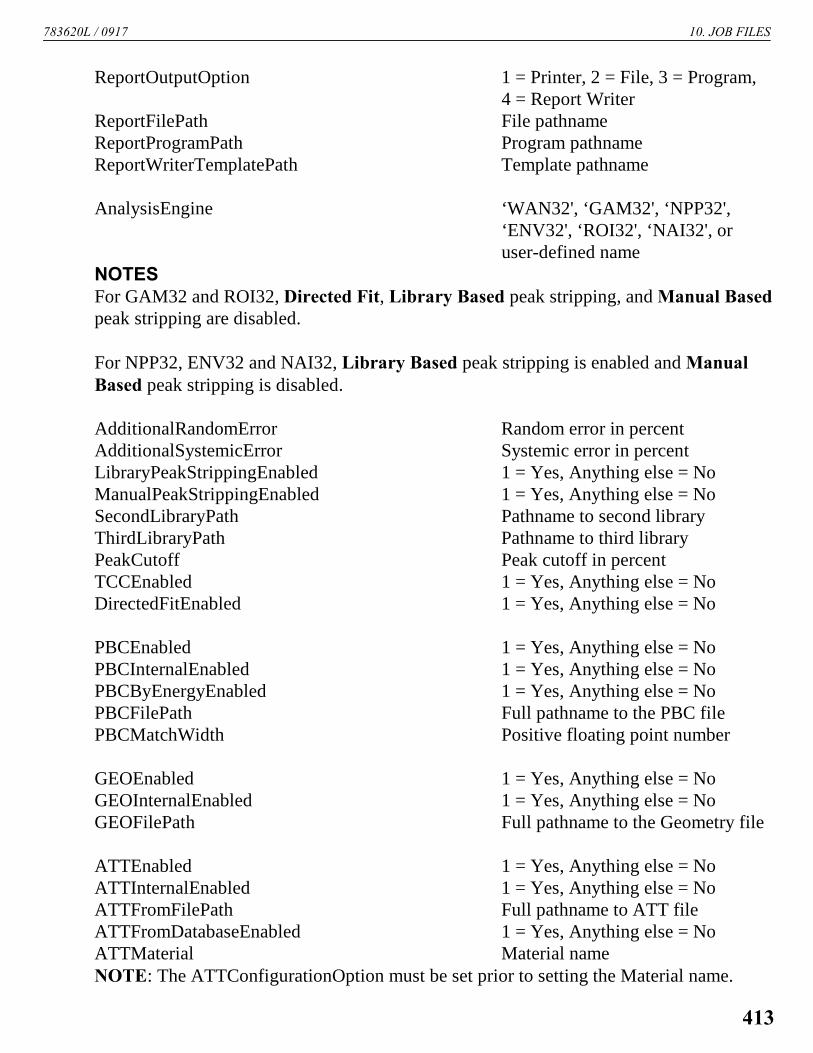
783620L / 0917 10. JOB FILES
ReportOutputOption 1 = Printer, 2 = File, 3 = Program,4 = Report Writer
ReportFilePath File pathnameReportProgramPath Program pathnameReportWriterTemplatePath Template pathname
AnalysisEngine ‘WAN32', ‘GAM32', ‘NPP32',‘ENV32', ‘ROI32', ‘NAI32', oruser-defined name
NOTESFor GAM32 and ROI32, Directed Fit, Library Based peak stripping, and Manual Basedpeak stripping are disabled.
For NPP32, ENV32 and NAI32, Library Based peak stripping is enabled and ManualBased peak stripping is disabled.
AdditionalRandomError Random error in percentAdditionalSystemicError Systemic error in percentLibraryPeakStrippingEnabled 1 = Yes, Anything else = NoManualPeakStrippingEnabled 1 = Yes, Anything else = NoSecondLibraryPath Pathname to second libraryThirdLibraryPath Pathname to third libraryPeakCutoff Peak cutoff in percentTCCEnabled 1 = Yes, Anything else = NoDirectedFitEnabled 1 = Yes, Anything else = No
PBCEnabled 1 = Yes, Anything else = NoPBCInternalEnabled 1 = Yes, Anything else = NoPBCByEnergyEnabled 1 = Yes, Anything else = NoPBCFilePath Full pathname to the PBC filePBCMatchWidth Positive floating point number
GEOEnabled 1 = Yes, Anything else = NoGEOInternalEnabled 1 = Yes, Anything else = NoGEOFilePath Full pathname to the Geometry file
ATTEnabled 1 = Yes, Anything else = NoATTInternalEnabled 1 = Yes, Anything else = NoATTFromFilePath Full pathname to ATT fileATTFromDatabaseEnabled 1 = Yes, Anything else = NoATTMaterial Material nameNOTE: The ATTConfigurationOption must be set prior to setting the Material name.
413

GammaVision® V8 (A66-BW) 783620L / 0917
ATTConfigurationOption 1 = Linear, Anything else = MassATTLength Length or MassATTTypeOption 1 = Internal, Anything else =
External
AvgEnergyEnabled 1 = Yes, Anything else = NoAvgEnergyInternalEnabled 1 = Yes, Anything else = NoAvgEnergyFilePath Full pathname to the .EBR file
IEQEnabled 1 = Yes, Anything else = NoIEQInternalEnabled 1 = Yes, Anything else = NoIEQFilePath Full pathname to the .IEQ file
DACEnabled 1 = Yes, Anything else = NoDACInternalEnabled 1 = Yes, Anything else = NoDACFilePath Full pathname to the .DAC file
GammaTotalReportingEnabled 1 = Yes, Anything else = NoGammaTotalGermaniumReportingEnabled 1 = Yes, Anything else = NoGammaTotalCalculationEnabled 1 = Yes, Anything else = NoGammaTotalEDFTableOnlyEnabled 1 = Yes, Anything else = NoGammaTotalReportIsoMdaOnReportsEnabled 1 = Yes, Anything else = NoGammaTotalCountBackgroundEnabled 1 = Yes, Anything else = NoGammaTotalCountCesiumEnabled 1 = Yes, Anything else = NoGammaTotalWriteBackgroundReportEnabled 1 = Yes, Anything else = NoGammaTotalWriteMaintenanceReportEnabled 1 = Yes, Anything else = NoGammaTotalSequence Integer numberGammaTotalGermaniumSequence Integer numberGammaTotalReportDirectory Directory pathGammaTotalGermaniumReportDirectory Directory pathGammaTotalAnalysisStartChannel Starting channel numberGammaTotalAnalysisEndChannel Ending channel numberGammaTotalUseRangeForBackgroundQAEnabled 1 = Yes, Anything else = NoGammaTotalBackgroundSpectrumPath Full pathnameGammaTotalCesiumSpectrumPath Full pathnameGammaTotalGeometryFilePath Full pathname
AdditionalUncertainty1Name String description 37 chars maxAdditionalUncertainty2Name String description 37 chars maxAdditionalUncertainty3Name String description 37 chars maxAdditionalUncertainty4Name String description 37 chars maxAdditionalUncertainty5Name String description 37 chars max
414
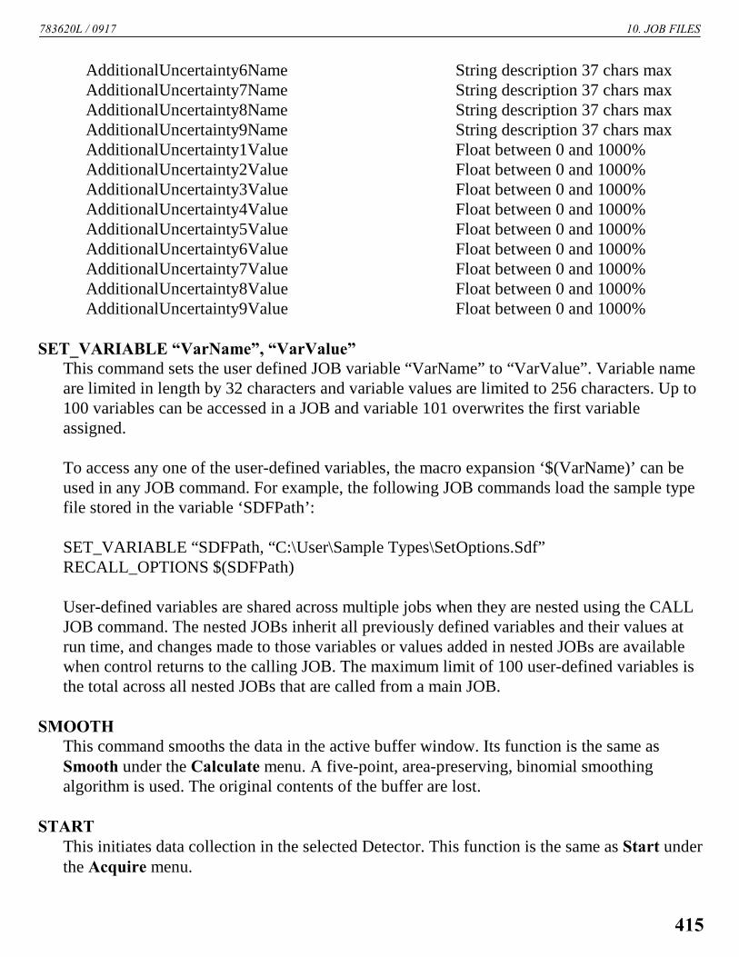
783620L / 0917 10. JOB FILES
AdditionalUncertainty6Name String description 37 chars maxAdditionalUncertainty7Name String description 37 chars maxAdditionalUncertainty8Name String description 37 chars maxAdditionalUncertainty9Name String description 37 chars maxAdditionalUncertainty1Value Float between 0 and 1000%AdditionalUncertainty2Value Float between 0 and 1000%AdditionalUncertainty3Value Float between 0 and 1000%AdditionalUncertainty4Value Float between 0 and 1000%AdditionalUncertainty5Value Float between 0 and 1000%AdditionalUncertainty6Value Float between 0 and 1000%AdditionalUncertainty7Value Float between 0 and 1000%AdditionalUncertainty8Value Float between 0 and 1000%AdditionalUncertainty9Value Float between 0 and 1000%
SET_VARIABLE “VarName”, “VarValue”This command sets the user defined JOB variable “VarName” to “VarValue”. Variable nameare limited in length by 32 characters and variable values are limited to 256 characters. Up to100 variables can be accessed in a JOB and variable 101 overwrites the first variableassigned.
To access any one of the user-defined variables, the macro expansion ‘$(VarName)’ can beused in any JOB command. For example, the following JOB commands load the sample typefile stored in the variable ‘SDFPath’:
SET_VARIABLE “SDFPath, “C:\User\Sample Types\SetOptions.Sdf”RECALL_OPTIONS $(SDFPath)
User-defined variables are shared across multiple jobs when they are nested using the CALLJOB command. The nested JOBs inherit all previously defined variables and their values atrun time, and changes made to those variables or values added in nested JOBs are availablewhen control returns to the calling JOB. The maximum limit of 100 user-defined variables isthe total across all nested JOBs that are called from a main JOB.
SMOOTHThis command smooths the data in the active buffer window. Its function is the same asSmooth under the Calculate menu. A five-point, area-preserving, binomial smoothingalgorithm is used. The original contents of the buffer are lost.
STARTThis initiates data collection in the selected Detector. This function is the same as Start underthe Acquire menu.
415

GammaVision® V8 (A66-BW) 783620L / 0917
The Ask on Start questions as defined in Acquire/Acquisition Settings... will be asked eachtime a START command is executed. This stops execution of the .JOB file until the questionis answered. If you choose Cancel for an ask-on-start prompt, the JOB terminates.
START_OPTIMIZEFor MCBs that support this feature, this starts the optimize function for the Detector. SeeSection 4.2.3.5 for functional details.
START_PZThis starts the PZ function for the detector. It is automatically included in the optimizefunction. This command is only available for MCBs with internal amplifiers.
STOPThis stops data collection in the active Detector. If the Detector has already been stopped, nooperation occurs. This command has the same function as Stop under the Acquire menu.
STOP_PZThis stops the PZ function for the detector. Note that the PZ function is not complete whenthis is used. The PZ function should be allowed to complete automatically. This command isonly available for MCBs with internal amplifiers.
STRIP <factor>,[“file.chn”]This strips the disk spectrum specified in the SET_NAME_STRIP command or in the com-mand itself (either way is acceptable; the filename is optional in this command) from thespectrum in the buffer and stores the results in the buffer. The disk and selected data memoryspectra must be the same size. The disk spectrum can be scaled up or down by <factor> (aconstant) or, if <factor> is zero, by the ratio of the live times of the two spectra. The filenamecan include any of the variables defined in Section 10.2.
UNLOCK “Pwd”This unlocks the current Detector using “Pwd” as the password.
VIEW “i”, [“Type”]This moves the “i”th stored spectrum to position 0 (i.e., makes it active in the view). Thiscommand is only valid in MCBs with Field Mode or buffers containing N42 files that havemultiple spectra. The optional “Type” argument specifies the spectrum type to view withvalid options of “Any”, “Background”, “TimeSlice”, “LongCount”, “KnownSample”, or“BlankSample”. Any other Type options will generate an error.
The Job variable “$(Spectra)” is updated to reflect the number of spectra stored in a multiplespectrum file when the VIEW command is run. This variable can be used with the LOOPcommand to automatically process each spectrum as necessary. An example Job showing
416
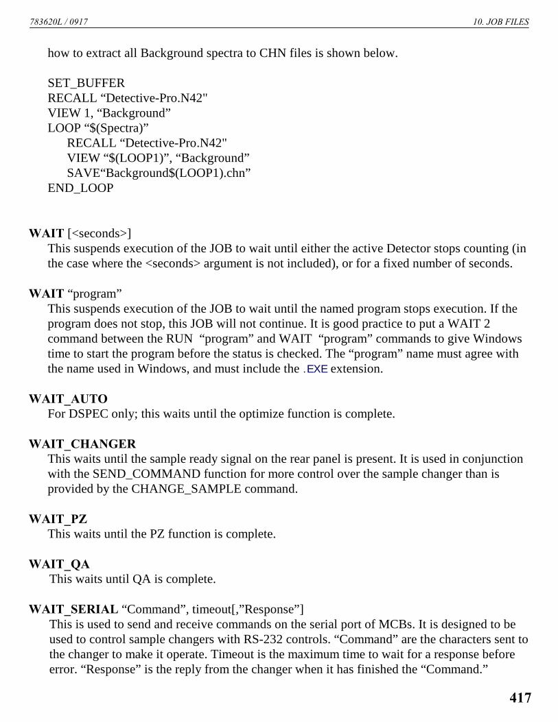
783620L / 0917 10. JOB FILES
how to extract all Background spectra to CHN files is shown below.
SET_BUFFERRECALL “Detective-Pro.N42"VIEW 1, “Background”LOOP “$(Spectra)”
RECALL “Detective-Pro.N42"VIEW “$(LOOP1)”, “Background”SAVE“Background$(LOOP1).chn”
END_LOOP
WAIT [<seconds>]This suspends execution of the JOB to wait until either the active Detector stops counting (inthe case where the <seconds> argument is not included), or for a fixed number of seconds.
WAIT “program”This suspends execution of the JOB to wait until the named program stops execution. If theprogram does not stop, this JOB will not continue. It is good practice to put a WAIT 2command between the RUN “program” and WAIT “program” commands to give Windowstime to start the program before the status is checked. The “program” name must agree withthe name used in Windows, and must include the .EXE extension.
WAIT_AUTOFor DSPEC only; this waits until the optimize function is complete.
WAIT_CHANGERThis waits until the sample ready signal on the rear panel is present. It is used in conjunctionwith the SEND_COMMAND function for more control over the sample changer than isprovided by the CHANGE_SAMPLE command.
WAIT_PZThis waits until the PZ function is complete.
WAIT_QAThis waits until QA is complete.
WAIT_SERIAL “Command”, timeout[,”Response”]This is used to send and receive commands on the serial port of MCBs. It is designed to beused to control sample changers with RS-232 controls. “Command” are the characters sent tothe changer to make it operate. Timeout is the maximum time to wait for a response beforeerror. “Response” is the reply from the changer when it has finished the “Command.”
417

GammaVision® V8 (A66-BW) 783620L / 0917
The first operation is to send “Command” out the serial port for the selected Detector. It thenwaits for a response or timeout according to these entries:
1. If a response string is provided, the length of the response string determines the exactnumber of characters to wait for.
2. If a response string is not provided, any character input will generate a success.3. If a response string is provided, and the characters do not match, an Invalid Response
message is generated and the JOB terminates.4. If a timeout occurs, a Timeout Message is generated and the JOB terminates.
Example:SET_DETECTOR 1LOOP 3
WAIT_SERIAL “$(Loop1)L$(CR)”, 300, “$(BEL)”BEEP 5
END_LOOP
This code does the following:1. Sends 1L5 and waits 5 minutes for an ASCII Bell Character. Beeps 5 after ASCII bell is
received.2. Sends 2L5 and waits 5 minutes for an ASCII Bell Character. Beeps 5 on success.3. Sends 3L5 and waits 5 minutes for an ASCII Bell Character. Beeps 5 on success.
The 5 is the $(CR) (carriage return) character.
ZOOM <i>Changes the size of the GammaVision window. Selects one of icon, normal, or maximumaccording to the argument. The arguments are:
!1 = minimize (icon on Taskbar) 0 = normal (size determined by last use)+1 = maximize (full screen)
ZOOM: <x,y,w,h>Changes the position and size of the GammaVision window. The arguments are:
x = x position of upper-left corner of window (0 is left)y = y position of upper-left corner of window (0 is top)w = width of window in pixels, starting at x and going righth = height in pixels, starting at y and going down
Since these arguments are in pixels, experimentation is the best way to determine the desiredsize.
418
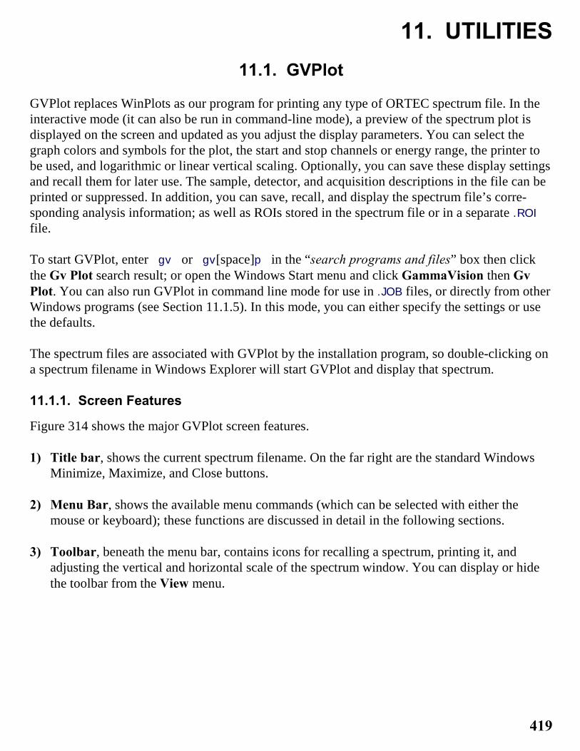
11. UTILITIES
11.1. GVPlot
GVPlot replaces WinPlots as our program for printing any type of ORTEC spectrum file. In theinteractive mode (it can also be run in command-line mode), a preview of the spectrum plot isdisplayed on the screen and updated as you adjust the display parameters. You can select thegraph colors and symbols for the plot, the start and stop channels or energy range, the printer tobe used, and logarithmic or linear vertical scaling. Optionally, you can save these display settingsand recall them for later use. The sample, detector, and acquisition descriptions in the file can beprinted or suppressed. In addition, you can save, recall, and display the spectrum file’s corre-sponding analysis information; as well as ROIs stored in the spectrum file or in a separate .ROI
file.
To start GVPlot, enter gv or gv[space]p in the “search programs and files” box then clickthe Gv Plot search result; or open the Windows Start menu and click GammaVision then GvPlot. You can also run GVPlot in command line mode for use in .JOB files, or directly from otherWindows programs (see Section 11.1.5). In this mode, you can either specify the settings or usethe defaults.
The spectrum files are associated with GVPlot by the installation program, so double-clicking ona spectrum filename in Windows Explorer will start GVPlot and display that spectrum.
11.1.1. Screen Features
Figure 314 shows the major GVPlot screen features.
1) Title bar, shows the current spectrum filename. On the far right are the standard WindowsMinimize, Maximize, and Close buttons.
2) Menu Bar, shows the available menu commands (which can be selected with either themouse or keyboard); these functions are discussed in detail in the following sections.
3) Toolbar, beneath the menu bar, contains icons for recalling a spectrum, printing it, andadjusting the vertical and horizontal scale of the spectrum window. You can display or hidethe toolbar from the View menu.
419

GammaVision® V8 (A66-BW) 783620L / 0917
Figure 314. The Main GVPlot Display.
4) The Expanded Spectrum Window shows all or part of the full histogram; this allows you tozoom in on a particular part of the spectrum and see it in more detail. You can change thevertical and horizontal scaling, and perform a number of operations such as displaying peakinformation, marking and modifying ROIs, and displaying the residuals (see item 6 below).This window contains a vertical line called a marker that highlights a particular position inthe spectrum. Information about that position is displayed on the Marker Information Line(see item 7 below). Right-clicking in this window opens a right-mouse-button menu, which isdiscussed in Section 11.1.4.
5) The Full Spectrum Window shows the full histogram from the file or the Detector memory.The vertical scale switches between logarithmic and linear in concert with the scaling in theexpanded window. When you zoom in on part of the spectrum in the expanded window, the
420

783620L / 0917 11. UTILITIES
Full Spectrum Window displays a rectangular area that reflects the portion of spectrum nowvisible in the Expanded Spectrum Window. To quickly move to different region in the spec-trum, either click that region in the Full Spectrum Window or click and drag the rectangle tothe new position, and the expanded display will update immediately at the new position. Youcan also zoom out by clicking and dragging a rubber rectangle over any portion of the FullSpectrum Window (the starting point for this operation must be outside of the currentexpanded-view indicator rectangle). The full-spectrum window can be moved and sized (seeSection 4.4.4).
6) Residuals, which can be displayed in the lower section of the spectrum window, displays acomparison of the counts in each channel to the calculated counts for that channel as deter-mined by the peak-fitting algorithm. This comparison can be displayed in counts (absoluteresiduals) or standard deviations (relative residuals). See the discussion on page 427.
7) Status Bar, below the Marker Information Line, displays program status information such aswarning messages. You can display or hide the status bar from the View menu.
8) Marker Information Line, beneath the spectrum, shows the Marker channel, markerenergy, and channel contents. The ROI section shows the boundaries of the ROI in energy(for calibrated spectra) or channels (for uncalibrated spectra), the number of counts in theROI, and other information; see the discussion associated with Fig. 326 on page 429.
11.1.2. The Toolbar
The row of buttons below the menu bar provides convenient shortcuts to some of the mostcommon GVPlot commands.
The Recall button retrieves an existing spectrum file. This is the equivalent of selecting
File/Recall Spectrum... from the menu.
Print sends the current spectrum immediately to the default Windows printer without
opening the standard Print dialog. If you wish to switch to another printer or adjust thedefault print properties, use the File/Print... command (Section 11.1.3.1).
Vertical Log/Lin Scale switches between logarithmic and linear scaling. When switching
from logarithmic to linear, it uses the previous linear scale setting.
Zoom In decreases the horizontal full scale of the Expanded Spectrum Window so the
peaks appear larger and broader. You can also access this command from the right-mouse-button menu (Section 11.1.4.2).
421

GammaVision® V8 (A66-BW) 783620L / 0917
Figure 315. The File Menu.
Figure 316. Open a Spectrum File.
Zoom Out increases the horizontal full scale of the Expanded Spectrum Window so the
peaks appear smaller and narrower. You can also access this command from the right-mouse-button menu (Section 11.1.4.3).
Center forces the marker to the center of the screen by shifting the spectrum without
moving the marker from its current channel.
Baseline Zoom sets and keeps the baseline of the Expanded Spectrum Window at zero
counts in Linear scale mode and 1.0E+0 counts in Logarithmic scale mode. When Base-line Zoom is off, the baseline can be offset to a higher value. This is useful to show smallpeaks on a high background.
11.1.3. Menu Commands
11.1.3.1. File
Figure 315 shows the File menu. Use these commands to select the spectrum, analysis, and ROIsto be displayed, recall or save GVPlot settings files, and print the spectrum.
Use the Recall Spectrum... command (Fig. 316) to open a spectrum file.
When the Show Description checkbox at the bottom of the dialog is marked, you can click eachspectrum filename and see its sample description, spectrum format, and number of channels asan aid in selecting the correct file.
422

783620L / 0917 11. UTILITIES
Figure 317. The Print Plot Dialog.
Figure 318.
Figure 319.
The recalled spectrum will be displayed using the most recently selected graph color, symbol,and axis-scaling settings (which are set with the Options/Graph... command). These settingswill also be used when you Print the spectrum or save it as a bitmap or jpeg image with SavePlot...
Once you have opened a spectrum file, Recall ROIs allows you to import the ROIs from an .ROI
file. You can also open the corresponding analysis results (.UFO) file with Recall UFO File.
The graph colors, symbols, and axis parameters selected in Options/Graph... can be saved in anASCII text file with the Save Settings As... command (which opens a standard Windows file-open dialog). The Recall Settings command allows you to recall a particular settings file so youcan quickly and reproducibly adjust the appearance of the spectrum window. You can also call asettings file from the GVPlot command line to ensure the resulting plot(s) will be displayedaccording to your specifications.
The Print... dialog (Fig. 317) allows youto select a printer Name and specify theNumber of copies to be printed (thisnumber is reset to 1 after every print ses-sion). Click Properties to change printoptions such as paper size, orientation,and output resolution.
11.1.3.2. View
Figure 318 shows the View menu, whichallows you to hide or display the Toolbarand Status Bar.
11.1.3.3. Options
The Options menu is shown in Fig. 21. These menu items govern the appearance of the spectrumwindow and printed output.
423

GammaVision® V8 (A66-BW) 783620L / 0917
Figure 320. The Plot Options Dialog.
Graph...
This command opens the dialog shownin Fig. 320, which lets you set the graphcolors, symbol type, and axis scalingfactors. These settings are stored whenyou exit GVPlot and reloaded the nexttime GVPlot is started. You can also savethese settings in an ASCII text file usingthe Save Settings As... command, andretrieve them with Recall Settings....Graph... is duplicated by the Properties itemon the right-mouse-button menu.
The droplists on the left side of thedialog control the screen and printoutcolors. As noted above, there are somedifferences between screen and printerfonts and colors. Also, if you do not havea color printer, the screen colors will berendered in grayscale.
The Text color affects the color of the axes, axis labels, and spectrum title. Background controlsthe color of the spectrum background in both the full and expanded windows. Markers appliesto the ROI bars.
Data Set Colors allows you to choose separate colors for spectrum Data, Fitted peaks, andResiduals; select a data type from the left-hand droplist, then choose a color from the list on theright. Similarly, use Fill Color to control the colors of ROIs, Nuclide Peaks, Unknown Peaks,Multiplets, and Composites in both point and fill modes. Spectrum Style determines how thehistogram data are represented (Points, Line, or Fill All).
The Show Nuclide Name checkbox allows you to hide or display the nuclide markers for ananalyzed spectrum (an example of these markers is shown in Fig. 20, page 26). Turning thenuclide markers on or off slightly adjusts the graph’s vertical scaling.
Clearing the Show Axes checkbox removes the axes so the portion of histogram shown in theExpanded Spectrum Window occupies the entire window without an inside border.
Set the Y Axis Scale of both the Full and Expanded Spectrum Windows to Linear or Logarith-mic. You can also do this with the Vertical Log/Lin Scale button on the toolbar.
424

783620L / 0917 11. UTILITIES
Figure 321. Draw Multiplet Modes.
The Draw Multiplet radio buttons determine whethermultiplets are drawn as a Composite curve, shownindividually (Each), or displayed as individual peakssuperimposed with the composite curve (Both). Thesemodes are compared in Fig. 321. This display is mosteasily seen with all Fill Modes turned off (checkboxesunmarked).
The Fill Mode checkboxes allow you to determinewhich peak types, if any, will be displayed in fill moderather than data-point mode.
Auto Y (Spectrum) allows you set up a fixed y-axisrange for the Expanded Spectrum Window (Auto Yunmarked/off), or allow the program to autoscale they-axis to accommodate the tallest peak currently displayed in the expanded view (Auto Ymarked/on). The Auto Y (Residual) functions similarly for the residuals plot (which is displayedfrom the right-mouse-button menu, Section 11.1.4.1).
If the spectrum is calibrated, the Horizontal axis can be displayed in either Energy units orChannel numbers. If the spectrum is not calibrated, the horizontal axis is shown in channels andcannot be changed.
You can plot all or part of a spectrum by turning Auto X Range respectively on or off. TurningAuto X Range off activates the x-axis range fields that allow you to let the plot limits in eitherchannels or keV (select units from the droplist). The plot limits are independent of the x-axisunits of measure. This means that you can, if you wish, choose to display the x-axis in Energyunits, then select the portion of the spectrum to be displayed as a range of channel numbers.
In order to easily compare spectra, the energy can be set to values below the first channel in thespectrum. In this case the data below channel 0 are plotted as 0.
NOTE Manually setting the range for one axis disables zooming for that axis only. If both axisranges are manually fixed, all zooming is disabled.
Title Text
This dialog (Fig. 322) allows you to compose a title to be displayed at the top of the spectrumplot. In addition, you can choose whether or not to display the Real and Live Time, SpectrumFile Name, and the sample or Detector description.
425

GammaVision® V8 (A66-BW) 783620L / 0917
Figure 322. Compose the Plot Title.
Figure 323. TheROI Menu.
Auto Load UFO
When this feature is turned on (a checkmark is dis-played beside the command), recalling aspectrum file also recalls the corresponding .UFO file if it shares the same filename and drive/folder location as the spectrum file. Note that if the analysis captured in the .UFO file covers onlypart of the spectrum, that portion of the spectrum, rather than the entire spectrum, will initially bedisplayed in the Expanded Spectrum View.
11.1.3.4. ROI
The ROI menu (Fig. 323) works in conjunction with the Mark ROI and Clear Active ROIcommands on the right-mouse-button menu (Section 11.1.4).
Modify Active ROI/Off
This enables the Modify Active ROI mode, which lets you use the left/right arrow keys to addmore channels to the currently active ROI (click inside the ROI to activate it). Pressing the leftarrow shifts the low-energy boundary of the ROI to the left and pressing the right arrow shiftsthe high-energy side to the right; this shift might take a moment to occur. As you adjust the sizeof the ROI, the ROI boundary (and ROI Bars, if currently displayed; see Section 11.1.4.8) shiftsand the Marker Information Line updates accordingly. When you select Off, the left/right arrowkeys return to their original function of moving the marker through the spectrum. You can alsoadjust the size of the ROI by clicking and dragging the ROI bars.
Clear
This clears the ROI bits in all ROI channels that adjoin the channel containing the marker. This isduplicated by the Clear Active ROI command on the right-mouse-button menu.
426

783620L / 0917 11. UTILITIES
Figure 324. TheContext Menu.
Clear All
This resets all the ROI bits in the spectrum, removing all ROI markings from the spectrum.
Save File...
This command allows you to save to disk a table of the channel numbers, for the current spec-trum, that have the ROI bit set. The contents of the spectrum are not changed. A standardWindows file-save dialog opens, allowing you to create a filename or overwrite an existing .ROI
file.
Recall File...
Recall File... sets the ROIs in the spectrum according to the table in the disk file created by ROI/Save File.... This command opens a standard file-open dialog, prompting you to select a file-name. When you select a file, the ROIs in the currently displayed spectrum are set to conform tothe table in the file. The previous ROIs are cleared. The spectrum data are not altered by thisoperation, only the ROI bits.
In .ROI files, the ROIs are saved by channel number. Therefore, if the spectrum peaks haveshifted in position, the ROIs in the file will not correspond exactly to the spectrum data.
11.1.4. Right-Mouse-Button (Context) Menu Commands
Figure 324 shows the right-mouse-button menu that openswhen you right-click in the Expanded Spectrum Window.
11.1.4.1. Show Residuals
Marking this menu item activates the Plot Absolute Residualsand Plot Relative Residuals modes. The Residuals section of thespectrum window (item 6 on page 421) displays a comparison ofthe counts in each channel (Actual) to the calculated counts forthat channel as determined by the peak-fitting algorithm (Fitted).Plot Absolute Residuals displays the difference in each channel,in counts, between Actual and Fitted counts. Plot RelativeResiduals displays the difference in each channel, in standarddeviations (abbreviated STD on the screen), between Actual andFitted counts divided by the square root of the Actual counts; thatis, .
The Properties command is equivalent to Options/Graph...;see Section 11.1.3.3.
427

GammaVision® V8 (A66-BW) 783620L / 0917
11.1.4.2. Zoom In
Zoom In adjusts the horizontal and vertical scales in the Expanded Spectrum Window to view asmaller portion of the spectrum. This command is duplicated by the Zoom In button on thetoolbar.
11.1.4.3. Zoom Out
Zoom Out adjusts the horizontal and vertical scales in the Expanded Spectrum Window to viewa larger portion of the spectrum. This command is duplicated by the Zoom Out button on thetoolbar.
11.1.4.4. Undo Zoom In
This will undo or reverse the last Zoom In operation done with the rubber rectangle. It restoresthe display to the horizontal and vertical expansion before the Zoom In. It is not the same asZoom Out.
11.1.4.5. Full View
Full View adjusts the horizontal and vertical scaling to display the entire spectrum in theExpanded Spectrum View.
11.1.4.6. Mark ROI
This allows you to mark a peak as an ROI by clicking and dragging the rubber rectangle across aportion of the spectrum, then selecting Mark ROI. If Show ROI Bars is on (Section 11.1.4.8),the new ROI will be marked with the active ROI Bars until you either move to or create anotherROI. Use the Modify Active ROI command on the ROI menu (Section 11.1.3.4) to widen theROI boundaries, or click and drag the ROI bars to increase or decrease the number of channels inthe ROI.
11.1.4.7. Clear Active ROI
This clears the ROI bits in all ROI channels that adjoin the channel containing the marker. This isthe same as the Clear command on the ROI menu (Section 11.1.3.4).
11.1.4.8. Show ROI Bars
These are vertical markers that indicate the lower and upper boundaries of each ROI in the spec-trum. The ROI bars for an inactive/unselected ROI have solid fill; when you click an ROI to acti-vate it (only one is active at a time), the bars for the active ROI change to a diagonal fill (seeFig. 325). To display the ROI bars, right-click in the expanded window to open the right-mouse-button menu, then click ROI Bars to checkmark it. To hide the ROI bars, click the commandagain to clear the checkmark.
428
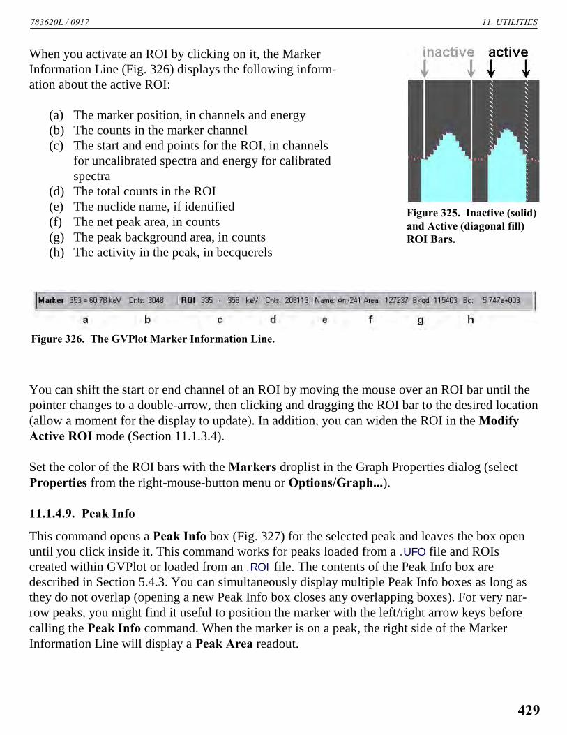
783620L / 0917 11. UTILITIES
Figure 325. Inactive (solid)and Active (diagonal fill)ROI Bars.
Figure 326. The GVPlot Marker Information Line.
When you activate an ROI by clicking on it, the MarkerInformation Line (Fig. 326) displays the following inform-ation about the active ROI:
(a) The marker position, in channels and energy(b) The counts in the marker channel(c) The start and end points for the ROI, in channels
for uncalibrated spectra and energy for calibratedspectra
(d) The total counts in the ROI(e) The nuclide name, if identified(f) The net peak area, in counts(g) The peak background area, in counts (h) The activity in the peak, in becquerels
You can shift the start or end channel of an ROI by moving the mouse over an ROI bar until thepointer changes to a double-arrow, then clicking and dragging the ROI bar to the desired location(allow a moment for the display to update). In addition, you can widen the ROI in the ModifyActive ROI mode (Section 11.1.3.4).
Set the color of the ROI bars with the Markers droplist in the Graph Properties dialog (selectProperties from the right-mouse-button menu or Options/Graph...).
11.1.4.9. Peak Info
This command opens a Peak Info box (Fig. 327) for the selected peak and leaves the box openuntil you click inside it. This command works for peaks loaded from a .UFO file and ROIscreated within GVPlot or loaded from an .ROI file. The contents of the Peak Info box aredescribed in Section 5.4.3. You can simultaneously display multiple Peak Info boxes as long asthey do not overlap (opening a new Peak Info box closes any overlapping boxes). For very nar-row peaks, you might find it useful to position the marker with the left/right arrow keys beforecalling the Peak Info command. When the marker is on a peak, the right side of the MarkerInformation Line will display a Peak Area readout.
429

GammaVision® V8 (A66-BW) 783620L / 0917
Figure 327. The Peak Info Window for anROI.
11.1.4.10. Show Hover Window
When you select this command, a checkmark is displayed by this menu item to indicate that it isin hover-window mode. In this mode, the Peak Info window opens when the mouse pointer ispaused over a peak for approximately 1 second, and closes when the pointer is moved away fromthe peak. To turn off hover mode, select Show Hover Window again to remove the checkmark.
11.1.4.11. Sum Spectrum
This sums the gross counts in the area selected with the rubber rectangle or, if you have notselected an area, the gross counts in the entire spectrum. The results are displayed on the statusline, and indicate the span of channels summed.
11.1.4.12. Print Graph
This command prints performs a “quick print” of the contents of the Expanded SpectrumWindow, using the currently selected printer and print settings (these will be either the defaultprinter and print settings for this computer or the printer and settings used most recently duringthis GVPlot session). To change printers and/or print properties, use the Print... command on theFile menu (page 423).
11.1.4.13. Properties
This opens the Graph Properties dialog, which is discussed in Section 11.1.3.3.
430

783620L / 0917 11. UTILITIES
11.1.5. Command Line Interface
The GVPlot command line interface supports options available in the interactive mode as shownbelow:
GvPlot <spectrum> -U <ufofile> -R <roifile> -S <setfile> -P
where:
<spectrum> Specifies the spectral data file (.SPC, .An1, or .CHN). The extension must beincluded.
-U <ufofile> Specifies the .UFO file. The extension must be included.
-R <roifile> Specifies the .ROI file. The extension must be included.
-S <setfile> Specifies the settings file. The extension must be included.
-P Print the plot to the PC’s Windows default printer and exit automatically.Used mainly in .JOB files and File/Export....
11.2. TRANSLT
The TRANSLT program (TRANSLT.EXE, located in your operating system’s program files folderunder \GammaVision) translates several different text files to and from .SPC or .CHN files. Alloperation is controlled from the command line. The command line is:
TRANSLT [-type] inname [[-type] outname] [-w] [-nc] [-col n] [-ni] [-nh] [-i]
where:
type chn The inname file is in CHN format.spc The inname file is in SPC format.txt The inname file is in ASCII text format.
The default is based on the filename extension and the i switch. Both chn and spc
cannot be used together.
inname The input spectrum file, no default; default extension is SPC. If the input file is a.TXT file, it must contain the live and real time in this format:
Real Time: 240.Live Time: 120
431

GammaVision® V8 (A66-BW) 783620L / 0917
Both values are in seconds.
The header information in the .TXT file will be converted and stored in the .SPC
file if it is in the correct format. The correct format for the .TXT input file is thesame as the .TXT format created as the output file.
type chn The outname file is in CHN format.spc The outname file is in SPC format.txt The outname file is in ASCII text format.
outname The output spectrum file. The default is the inname with the extension changed. Ifthe outname is not given, the spectrum file will not be overwritten by the defaultname. The length of the spectrum file converted from text will be the next higherpower of two with the surplus channels set to 0.
w Set the format output to 128 characters per line; default is 70 characters per line.
nc Do not print channel as first number in line; default is to print the channel number.The channel number is followed by a colon ( : ) to separate it from the data.
col n Number of data columns is n; default is 5. Error returned if line width will exceedavailable space.
ni Do not write acquisition or analysis information in output file; default is to writethis information.
nh Do not write header information in output file; default is to write this information.
i Import a text file and save as .SPC (or .CHN) file. If one filename is given, defaultis to convert that file to the other format, i.e., for AAA.SPC; the output will beAAA.TXT. If two filenames are given, the default is to convert the spectrum to text.The .TXT file will be overwritten even if the .SPC file is not located.
Example:
TRANSLT -SPC GOODSPEC -TXT TEXTSPEC -ni -nh -col 1
This will make a text file of one column with no header, no analysis information, and onechannel per line.
432

Figure 328. GammaVisionMenu.
APPENDIX A. STARTUP AND CONFIGURATIONOPTIONS
To start GammaVision, enter gamm in the “search pro-grams and files” box then click the GammaVision searchresult; or open the Windows Start menu and click Gamma-Vision, and GammaVision (Fig. 328). You can also startGammaVision by entering run in the search box andchoosing the Run search result; or (in XP) by selectingRun... from the Start menu. The Run option allows you tostart up from the command line, with or without arguments,as described below.
A.1. Command Line Options
GammaVision is run with the following command line properties:
GV32 [-d[n]] [-L file.lib] [-p listname] [-t] [-l] [-B] [-z] [file.job]
All of the arguments are optional; one or more can be omitted. Thus, at a minimum, Gamma-Vision can be executed without any arguments at all, in which case certain defaults apply for theDetector list and nuclide library, as described below. Switches (e.g., -d, -z) can be uppercase orlowercase (e.g., -d or -D, -z or -Z).
[n] An optional parameter for the -d switch to enable debugging output mode at aspecified level (values are 1 or 2; no argument is equivalent to 1). Default is nodebugging. Debug mode is not recommended for general use.
file.lib An optional nuclide library (use with -L option) to be loaded at startup. The defaultis the library loaded when GammaVision exited.
-p listname Optionally uses listname as the Detector pick list name. The pick list name must be5 characters or less. If a pick list is not specified, M32MCA.CFG — located inC:\ProgramData\ORTEC Shared\UMCBI — is used by default. The current pick listname is displayed above the Pick List column in the Detector List Editor dialog
433

GammaVision® V8 (A66-BW) 783620L / 0917
(Services/Edit Detector List...). If the pick list name specified by pick does notexist then one is created. This new list will contain all available detectors includedin the Master Detector List. If the pick list already exists, only the detectors definedin that list are displayed in the Detector droplist on the toolbar. Changes made tothe pick list with the Edit Detector List... command are stored with the active picklist filename. Therefore, to create multiple pick lists, use the -p option with the picklist name and then edit the list to contain only the desired Detectors. The contentsof the list can be overridden with the Edit Detector list function. The new list willbe stored for use the next time this instance of GammaVision is run.
-t Forces GammaVision to be “Always on Top.” The default is the normal Windowsdisplay.
-1 Allows one and only one instance to run. This is the numeral one.
-B Start up with an open buffer window. This should be used if the computer is on anetwork and no MCBs are connected anywhere in the system.
-z The “zoom” switch with several variations:
-z or -z: With no arguments, causes the previously stored “ZOOM:”parameters (see page 417) to be used to position and size theGammaVision window.
-z:x,y,w,h Changes the position and size of the GammaVision window. Thearguments (which are the same as for the ZOOM: profilevariables, page 417) are:
x = x position of upper-left corner of window (0 is left)y = y position of upper-left corner of window (0 is top)w = width of window in pixels, starting at x and going righth = height in pixels, starting at y and going down
-z0 Forces position and size to be determined by Windows tilingalgorithm.
-z+1 Forces GammaVision to be maximized.
-z-1 Forces GammaVision to be minimized (icon).
file.job An optional .JOB file to be executed at start-up.
434
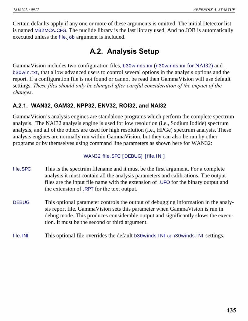
783620L / 0917 APPENDIX A. STARTUP
Certain defaults apply if any one or more of these arguments is omitted. The initial Detector listis named M32MCA.CFG. The nuclide library is the last library used. And no JOB is automaticallyexecuted unless the file.job argument is included.
A.2. Analysis Setup
GammaVision includes two configuration files, b30winds.ini (n30winds.ini for NAI32) andb30win.txt, that allow advanced users to control several options in the analysis options and thereport. If a configuration file is not found or cannot be read then GammaVision will use defaultsettings. These files should only be changed after careful consideration of the impact of thechanges.
A.2.1. WAN32, GAM32, NPP32, ENV32, ROI32, and NAI32
GammaVision’s analysis engines are standalone programs which perform the complete spectrumanalysis. The NAI32 analysis engine is used for low resolution (i.e., Sodium Iodide) spectrumanalysis, and all of the others are used for high resolution (i.e., HPGe) spectrum analysis. Theseanalysis engines are normally run within GammaVision, but they can also be run by otherprograms or by themselves using command line parameters as shown here for WAN32:
WAN32 file.SPC [DEBUG] [file.INI]
file.SPC This is the spectrum filename and it must be the first argument. For a completeanalysis it must contain all the analysis parameters and calibrations. The outputfiles are the input file name with the extension of .UFO for the binary output andthe extension of .RPT for the text output.
DEBUG This optional parameter controls the output of debugging information in the analy-sis report file. GammaVision sets this parameter when GammaVision is run indebug mode. This produces considerable output and significantly slows the execu-tion. It must be the second or third argument.
file.INI This optional file overrides the default b30winds.INI or n30winds.INI settings.
435

GammaVision® V8 (A66-BW) 783620L / 0917
Figure 329. The b30winds.ini File in Notepad.
A.2.2. B30winds.ini and N30winds.ini
The b30winds.ini file (Fig. 329) contains global analysis settings for all HPGe analysis engines. The NAI32 analysis engine has the same parameters in the n30winds.ini to allow for differentsettings associated with low resolution spectrum analysis.
If the specified file cannot be found in the same directory as the analysis engine then the\MESSAGE directory on the default drive is searched. If it is not found there or cannot be read,then the internal values are used.
NOTE These parameters are read sequentially from the file and none can be omitted even ifthey will not be used. Doing so would offset the parameters, and subsequent settingswould be incorrectly interpreted.
A.2.2.1. Contents
Except where indicated, all discussion of analysis settings refers to the current (working) settingson the Analyze/Settings/Sample Type... tabs or in the selected .SDF file.
436

783620L / 0917 APPENDIX A. STARTUP
Message file nameB30WIN.TXT The name of the file that defines the standard analysis report format.
spellingsYES NO Spelling of Yes and No displayed on analysis report under the
Corrections Status column. Alternates to English can be substituted.
spellings of monthsNO LONGER USED.
Deconvol. characterD The character in the peak tables indicating that this peak is part of a
deconvolution.
Shape characters Bad-peak-shape indicator in the peak tables.
Multiplet characterM The peak table character indicating this peak is part of a multiplet.
Unknown suspectS The character in the unknown peak table indicating that this peak was
not found in the Suspect Library.
EBAR table filenameC:\User\EBAR.TBL Filename for the average energy table. The analysis setting overwrites
this parameter in most cases. (Included for backward compatibilitywith older spectrum formats. This setting is used when analyzing .CHN
spectra using the Analyze/ Spectrum on Disk... command or when theanalysis is performed external to GammaVision.)
IEQ table filenameC:\User\IEQT.TBL Filename for the iodine equivalence table. The analysis setting over-
writes this parameter in most cases. (Included for backward compati-bility with older spectrum formats. This setting is used when analyzing.CHN spectra using the Analyze/ Spectrum on Disk... command orwhen the analysis is performed external to GammaVision.)
437

GammaVision® V8 (A66-BW) 783620L / 0917
EBAR on/offF Average Energy flag. The analysis setting overwrites this parameter in
most cases. (Included for backward compatibility with older spectrumformats. This setting is used when analyzing .CHN spectra using theAnalyze/ Spectrum on Disk... command or when the analysis isperformed external to GammaVision.)
T = Perform average energy calculation.F = Do not perform average energy calculation.
IEQ on/offF Iodine Equivalence flag. The analysis setting overwrites this parameter
in most cases. (Included for backward compatibility with older spec-trum formats. This setting is used when analyzing .CHN spectra usingthe Analyze/ Spectrum on Disk... command or when the analysis isperformed external to GammaVision.)
T = Perform iodine equivalence calculationF = Do not perform iodine equivalence calculation
Unidentified Peak Summary and Library Peak Usage Format flagT
T = Print efficiency corrected peak area for unknown peaks instead of net peak count rate andinclude the nuclide half-life and peak branching ratios in the Library Peak Usage section.F = Print net peak count rate for unknown peaks instead of efficiency corrected peak area andomit the nuclide half-life and peak branching ratios in the Library Peak Usage section.
Minimum Good Peaks Above Dividing Energy for Energy Recalibration (5 Minimum)1000 This flag does not function in ROI32. Number of good peaks above the
energy calibration dividing point required for an automatic energyrecalibration during analysis. The maximum value is 9999.
Minimum Good Peaks Below Dividing Energy for Energy Recalibration (5 Minimum)1000 This flag does not function in ROI32. Number of good peaks below the
energy calibration dividing point required for an automatic energyrecalibration during analysis. The maximum value is 9999.
Energy Recalibration Dividing Energy0.0 This flag does not function in ROI32. Energy calibration dividing point
(energy). This value must include a decimal point.
438

783620L / 0917 APPENDIX A. STARTUP
Activity Scaling Factor1.0 Scaling factor multiplied times nuclide activity in addition to the
Multiplier, Divisor, and Weight values specified in the analysissettings. This value must include a decimal point.
Unidentified Peak Match Width Factor2.0 Range multiplier for listing suspect nuclides in the unknown peak
table. For peaks listed in the unknown peak table, the suspect nuclidein the unknown peak table is determined by choosing the closestenergy match to the unknown peak that is within Range Multiplier *FWHM of each peak. This value must include a decimal point.
Page length60 Page length (in lines) of analysis report.
Save UFO File flagT If the .UFO file is deleted upon completion of the analysis, some
features in GVPlot, the Display Analysis Results... command, andupdating PBC files will not be not available because these functionsrely on information stored in the .UFO file.
T = Do not delete .UFO file after analysis is complete.F = Erase .UFO file after analysis is complete.
MDA Type, T = Allow change1 T
T = Allow change and use the MDA Type specified in the analysis settings.F = Do not allow change and always use the MDA number specified on this line, regardlessof the analysis settings. The MDA number is based on the order in which MDA methods arelisted on the System tab.
PBC F=off and filenameF PBCTEST.PBC
T = Use the PBC file specified here unless a different PBC file is given in the analysis set-tings. The file must include the full path and is limited to 32 characters total.F = Do not use a PBC file unless one is specified in the analysis settings.
439
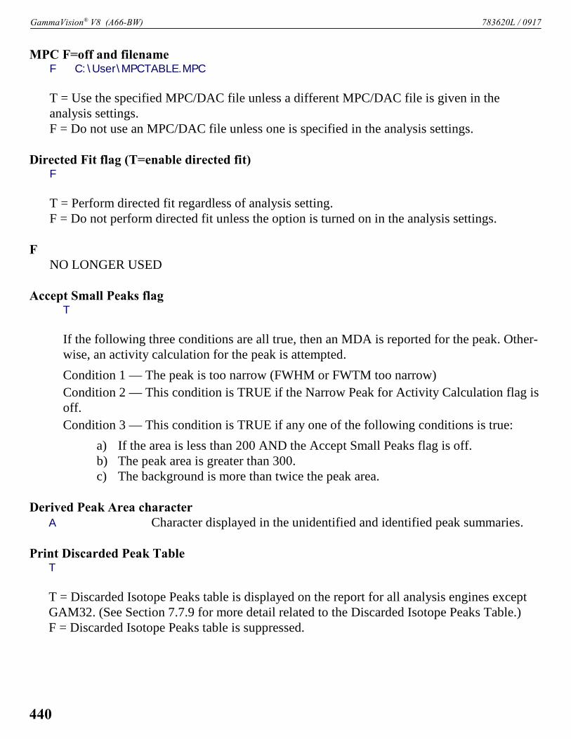
GammaVision® V8 (A66-BW) 783620L / 0917
MPC F=off and filenameF C:\User\MPCTABLE.MPC
T = Use the specified MPC/DAC file unless a different MPC/DAC file is given in theanalysis settings.F = Do not use an MPC/DAC file unless one is specified in the analysis settings.
Directed Fit flag (T=enable directed fit)F
T = Perform directed fit regardless of analysis setting.F = Do not perform directed fit unless the option is turned on in the analysis settings.
FNO LONGER USED
Accept Small Peaks flagT
If the following three conditions are all true, then an MDA is reported for the peak. Other-wise, an activity calculation for the peak is attempted.
Condition 1 — The peak is too narrow (FWHM or FWTM too narrow)
Condition 2 — This condition is TRUE if the Narrow Peak for Activity Calculation flag isoff.
Condition 3 — This condition is TRUE if any one of the following conditions is true:
a) If the area is less than 200 AND the Accept Small Peaks flag is off.b) The peak area is greater than 300.c) The background is more than twice the peak area.
Derived Peak Area characterA Character displayed in the unidentified and identified peak summaries.
Print Discarded Peak TableT
T = Discarded Isotope Peaks table is displayed on the report for all analysis engines exceptGAM32. (See Section 7.7.9 for more detail related to the Discarded Isotope Peaks Table.)F = Discarded Isotope Peaks table is suppressed.
440

783620L / 0917 APPENDIX A. STARTUP
Maximum Half-lives Cutoff12 The Decay-Corrected Activity is flagged as exceeding the half-life cutoff
instead of calculating a decay-corrected activity value. The same type offlag is displayed in the Summary of Peaks in Range section. Themaximum value is 9999.
Peak Activity Range Factor2.
This is the uncertainty multiplier used in determining the acceptable activity range perSection 6.7.1. This value must be followed by a decimal point.
Activity Range Test flagT
T = Use the Activity Range Factor in the previous parameter to determine if a nuclide peak isused to calculate the weighted average nuclide activity.F = Use all peaks that meet the uncertainty cutoff in determining the weighted averagenuclide activity.
Zero Area Identified Peak flagF
T = Show peaks that are not found in the spectrum (i.e., fail the Peak Cutoff test) in theIdentified Peak Summary with the following qualifications for specific analysis engines:
! WAN32 and ROI32 — Peak data is displayed for all peaks in the library.
! GAM32 — Peak data is displayed for all peaks reported, but all library peaks may notbe reported depending on peak quality, library content, and analysis settings.
! NPP32 — Deconvoluted peaks that are rejected may not be included in the peak list. Only the peak background and FWHM is displayed for peaks that do not meet the peakcutoff criteria.
! ENV32 and NAI32 — Some rejected peaks may be included in the list, but no peakdata are displayed.
F = Only show peaks in the Identified Peak Summary that meet the Uncertainty cutoff limit.
Zero Activity Isotope flagF This flag functions only for the NPP32, ENV32, and NAI32 analysis
engines. The GAM32, WAN32, and ROI32 analysis engines show allnuclides (even if zero activity) regardless of this flag setting.
T = Show nuclides with no activity reported in the Summary of Library Peak Usage table.This would include all nuclides in the library that were not found during analysis.
441

GammaVision® V8 (A66-BW) 783620L / 0917
F = Only show nuclides in the Summary of Library Peak Usage table that were identified inthe analysis. This includes nuclides that had zero activity because the associated peaks werefound but moved to the Discarded Peaks Table.
Minimum Step Background Energy0.0 Sets the lowest energy to use for a stepped background under a multiplet.
Typically, this parameter is set greater than zero only when multipletpeaks are found on the rising edge of a peak or continuum that is not com-patible with the stepped-background fitting methodology required for fit-ting small peaks on the high side of larger peaks. This value must includea decimal point.
Fraction Limit Test flagT This flag functions only in ENV32 and NAI32.
T = All nuclide peaks are used for the fraction limit test.F = Nuclide peaks flagged as “do not include in the average activity” in the library are notused for the fraction limit test.
Use Narrow Peaks for Nuclide Activity flagT Operates in conjunction with the “Accept Small Peaks” flag (page 440).
Zero Area Library Peak flagT This flag applies only to the NPP32, ENV32, and NAI32 analysis engines.
The WAN32, GAM32, and ROI32 analysis engines always display alllibrary peaks.
T = Show peaks with no area in the Summary of Library Peak Usage table. This wouldinclude all library peaks that did not pass the analysis settings criteria.F = Only show peaks in the Summary of Library Peak Usage table that passed the analysissettings criteria, and summarize how many library peaks were found as compared to the num-ber listed in the library for that nuclide (i.e., “X of Y peaks found”) under nuclide peak list.
442

783620L / 0917 APPENDIX A. STARTUP
Use Peak Cutoff flagT
T = Use Peak Cutoff specified in the analysis settings file to limit peaks used in the analysisto only those that meet the Peak Uncertainty Cutoff limit. F = Ignore the Peak Cutoff value in the analysis settings and use all peaks found regardless ofuncertainty in the analysis.
Second MDA type, T=Calculate2 T Second MDA Type (see MDA Type above). If set to T, the second MDA
type is stored in the .UFO file but it is not printed on the analysis report.
Sort Nuclide Peaks By Energy flagF This flag applies only to the WAN32, GAM32, and ROI32 analysis
engines. The NPP32, ENV32, and NAI32 analysis engines always sortpeak energy by the library order.
T = Sort peaks in the Summary of Library Peak Usage table by energyF = Sort peaks in the Summary of Library Peak Usage table by library order.
Multiplet channel shift limit2.0 The maximum number of channels that multiplet peaks can be shifted in
the peak-fit optimization. This value must include a decimal point.
Background width/FWHM for MDAs0.0 Use this value times the peak FWHM to determine the background area
for calculating the MDA. If set to zero, the entire background area for thepeak is used to calculate the MDA. (Use zero for old method.) This valuemust include a decimal point.
Print MDA in Nuclide Summary (T=Print MDA)T This parameter does not function in GAM32. GAM32 does not report
MDA for nuclides that have an activity value calculated.
T = Include the MDA in the Summary of Nuclides in Sample table when a nuclide activityvalue is calculated. F = The nuclide MDA is not included in the Summary of Nuclides in Sample table when anuclide activity is calculated.
443

GammaVision® V8 (A66-BW) 783620L / 0917
Maximum Half-life to Unknowns flagF
T = Treat peaks associated with nuclides exceeding the half-life limit as unknowns.F = Treat peaks associated with nuclides that exceed the half-life limit as identified peaksrather than unknowns.
Nuclide Summary MDA HeaderMDA MDA column header in “Summary of Nuclides in Sample” section of
report. This column header is displayed only if the nuclide MDA columnis included in the Summary of Nuclides in Sample table (see the “PrintMDA in Nuclide Summary” flag above).
ENV factor0.0 This flag functions only in ENV32, GAM32, and NAI32. Nuclide rejection
factor. In the library reduction algorithm, it is used to remove nuclidesfrom the analysis library. If set to a lower value, more nuclides will likelybe removed/dropped from the library (see Section 6.2.3 for details on howthis factor is used). This value must include a decimal point.
ISO NORM Probability alpha0.05 Probability variable á for the ISO NORM calculations. See also the
“b30winds.ini” discussion on page 157. This value must include a decimalpoint.
ISO NORM Probability beta0.05 Probability variable â for the ISO NORM calculations. See also the
“b30winds.ini” discussion on page 157. This value must include a decimalpoint.
ISO NORM Probability gamma0.05 Probability variable ä for the ISO NORM calculations. See also the
“b30winds.ini” discussion on page 157. This value must include a decimalpoint.
ISO NORM Print MDA flag T T = Report the MDA if the critical level is greater than the activity.
F = Always report the activity and the associated uncertainty.
444

783620L / 0917 APPENDIX A. STARTUP
Maximum ISO NORM MDA Ratio factor3.0 The maximum ratio of ISO NORM Detection Limit (MDA) to ISO
NORM Decision Threshold (Critical Level). This ratio is used to calculatethe “fmax” term, which limits the maximum ISO NORM Detection Limit(MDA); see page 316. This value must include a decimal point.
Peak overlap range in units of peak FWHM3.5 Peaks within FWHM times the Peak Overlap Range Factor plus peak
background points are deconvoluted. This value must include a decimalpoint. The minimum value is 1.0. Default for n30winds.ini is 2.0.
Directed Fit Minimum Background Counts for Quadratic Peak FitNO LONGER USED
Directed Fit Peak Region Width Factor1.00 Range factor used in the Directed Fit peak width determination. See
Section 6.3.2.2. This value must include a decimal point. The maximumvalue is 9999.
Dominant Background Peak Cutoff and Override flag25.0 T If the peak uncertainty exceeds this value at 1 sigma, then background
dominates with regard to the next two parameters below. The flag, Trueby default, specifies whether to override this value with the Peak Cutofffrom the analysis options (i.e., same criterion as acceptable peakdetermination). To set a different criterion for Dominant Background, setthe flag to False and specify the Dominant Background peak cutoffcriterion. This value must include a decimal point.
Dominant Background Peak Width Factor and flag1.20 T FWHM multiplier dictates the peak integration range (i.e., 1.2 * FWHM)
when background is dominant. When the flag is set to True, the fixedwidth factor is used to determine peak background when the peak is notpart of a multiplet. When the flag is set to False, the background isdetermined by the normal GammaVision peak integration calculation. The fixed width background is typically more representative whenbackground is dominant. This value must include a decimal point.
445

GammaVision® V8 (A66-BW) 783620L / 0917
Non-dominant Background Peak Width Factor and flag4.5 F FWHM multiplier dictates the peak integration range (i.e., 4.5 * FWHM)
when background is not dominant. When the flag is set to True, the fixedwidth factor is used to determine peak background when the peak is notpart of a multiplet. When the flag is set to False, the background isdetermined by the normal GammaVision peak integration calculation. The GammaVision peak integration is typically more representative whenbackground is not dominant (i.e., when peaks meet the acceptancecriteria). This value must include a decimal point.
TCC Internal Library FlagF T = Use Internal TCC Library Peaks
F = Use only peaks from the library in the analysis
Regional Decimal SettingsT T = Use decimal symbol in Regional Settings.
F = Use period for the decimal symbol regardless of Regional Settings.
511 kev Peak Centroid Tolerance1.0 Peaks with a centroid in the range of 511 kev plus or minus this tolerance
factor (in kev) use a FHWM wider than the calibration for the peak fit.
Library Nuclide Reduction Flag (GAM32, ENV32, and NAI32 Only)T T = Remove nuclides from the analysis that fail the key line or fraction
limit test based on the initial Mariscotti Peak Search. The ENV Factortest is unaffected by this setting. (Default for b30winds.ini)F = Library Nuclide Reduction by Key Line and Fraction Limit tests aredisabled (Default for n30winds.ini)
Library Peak Reduction Flag (GAM32, ENV32, and NAI32 Only)T T = If the Library Nuclide Reduction Flag is set to True, then remove any
peaks not found by the initial Mariscotti Peak Search from the analysis.F = Library Peak Reduction is disabled (Default)
Library Peak Critical Level Test Flag (GAM32, ENV32, and NAI32 Only)T T = Secondary nuclide peaks that have a calculated area based on the
nuclide average which is less than the calculated critical level at thatenergy will not be associated with the target nuclide. (Default forb30winds.ini)F =Peaks will be associated with a nuclide even if the peak area isexpected to be less than the critical level based on the average nuclideactivity. (Default for n30winds.ini)
446

783620L / 0917 APPENDIX A. STARTUP
Non-Directed Fit Maximum Activity Range100.0 This is the maximum activity range specified as a percentage of the first
peak activity when Directed Fit is not enabled in the analysis settings. Avalue of zero disables the maximum range test. (See Section 6.7.1.)
Directed Fit Maximum Activity Range0.0 This is the maximum activity range specified as a percentage of the first
peak activity when Directed Fit is enabled in the analysis settings. Avalue of zero disables the maximum range test. (See Section 6.7.1.)
447

GammaVision® V8 (A66-BW) 783620L / 0917
[Intentionally blank]
448

APPENDIX B. FILE FORMATS
This appendix describes the file structure for the GammaVision program files. See the ORTECSoftware File Structures Manual for DOS and Windows Systems for complete descriptions of theformats for these files, including .SPC, .CHN, and .UFO files. The .LIS file format is instrument-specific; see the hardware manual for your MCB. The .SPE file format is based on the IAEAASCII file format recommendation for gamma spectrometers; see the File Structures Manual fordetails.
B.1. GammaVision File Types
B.1.1. Detector Files
.CFG “ConFiGuration”; System Detector configuration information used by GV32.EXE; binaryformat.
.CXT “ConteXT”; For each Detector/Device a context file is automatically created to rememberall extra information required for analyses and calibration; binary format.
.SDF “Sample type defaults”; Created by the Analyze/Settings/Sample Type... command;binary format.
B.1.2. Spectrum Files
.CHN “CHaNnels”; MAESTRO-style spectral data file; binary format.
.SPC “SPeCtrum”; spectrum with full analysis settings, calibration, descriptions, etc; “Inform”type binary format.
.AN1 Alternate name for spectrum files used for analysis, when the .SPC name is already inuse; same format as .SPC.
B.1.3. Miscellaneous Files
.CLB “CaLibration”; full energy/efficiency calibration; “Inform” style binary format.
.LIB “LIBrary”; nuclide library; “Inform” style binary format.
.ROI “ROI”; channel pairs created by the ROI/Save File... function; binary format.
.UFO “UnFormatted Output”; analysis results; “Inform” style binary format.
449

GammaVision® V8 (A66-BW) 783620L / 0917
.EFT “EFficiency Table”; used for efficiency Calibrate/Recall Calibration... function (andcreated with the Save... button on the Efficiency Calibration Sidebar); formatted ASCIItext (also, lines that do not begin with numeric values are ignored).
.ENT “ENergy Table”; used for energy Calibrate/Recall Calibration... function (and createdwith the Save... button on the Energy Calibration Sidebar); formatted ASCII text (also,lines that do not begin with numeric values are ignored).
.RPT “RePorT”; output of analysis engine; ASCII text.
.TXT “TeXT”; general ASCII text files used by File/Print....
.JOB ASCII text providing commands for Services/JOB Control... function.
.DAC “Derived Activity Calculation”; values for the DAC or MPC calculation.
.EBR Average energy tables for the EBAR calculation.
.ATT “ATTenuation” database files.
.GEO “GEOmetry correction”; used for geometry correction function.
.IEQ “Iodine EQuivalence”; table values for the IEQ calculation.
.PBC “Peak Background Correction”; table values for the PBC.
B.1.4. QA Database Files
.MDB Microsoft Access database file extension.
B.2. Database Tables for GammaVision QA
B.2.1. QA Detectors Detector Table
(Only one of these tables for entire database; one record for each detector being monitored forQA, with fields defined as follows.)
Field Name SQL Data Type Description
Detector SQL_INTEGER Detector ID number. (Primary Key)
DetName SQL_CHAR (32) Detector Pick List Name
DetDesc SQL_CHAR (64) Detector Description
450
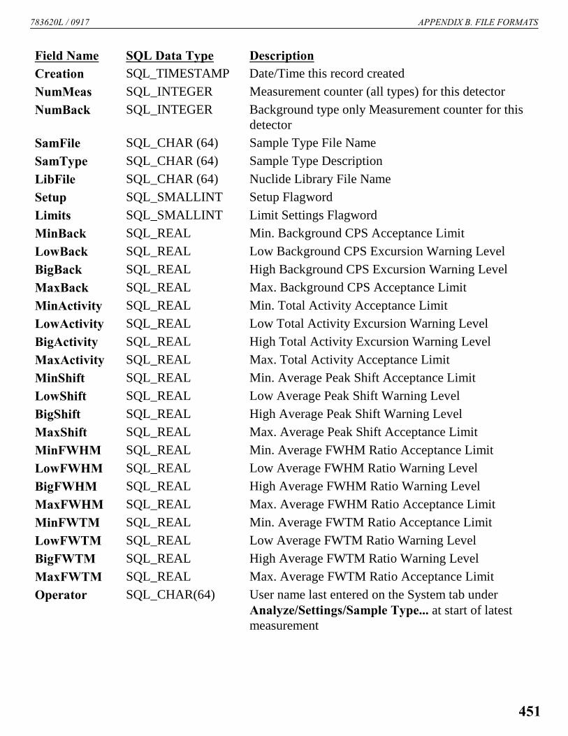
783620L / 0917 APPENDIX B. FILE FORMATS
Field Name SQL Data Type Description
Creation SQL_TIMESTAMP Date/Time this record created
NumMeas SQL_INTEGER Measurement counter (all types) for this detector
NumBack SQL_INTEGER Background type only Measurement counter for thisdetector
SamFile SQL_CHAR (64) Sample Type File Name
SamType SQL_CHAR (64) Sample Type Description
LibFile SQL_CHAR (64) Nuclide Library File Name
Setup SQL_SMALLINT Setup Flagword
Limits SQL_SMALLINT Limit Settings Flagword
MinBack SQL_REAL Min. Background CPS Acceptance Limit
LowBack SQL_REAL Low Background CPS Excursion Warning Level
BigBack SQL_REAL High Background CPS Excursion Warning Level
MaxBack SQL_REAL Max. Background CPS Acceptance Limit
MinActivity SQL_REAL Min. Total Activity Acceptance Limit
LowActivity SQL_REAL Low Total Activity Excursion Warning Level
BigActivity SQL_REAL High Total Activity Excursion Warning Level
MaxActivity SQL_REAL Max. Total Activity Acceptance Limit
MinShift SQL_REAL Min. Average Peak Shift Acceptance Limit
LowShift SQL_REAL Low Average Peak Shift Warning Level
BigShift SQL_REAL High Average Peak Shift Warning Level
MaxShift SQL_REAL Max. Average Peak Shift Acceptance Limit
MinFWHM SQL_REAL Min. Average FWHM Ratio Acceptance Limit
LowFWHM SQL_REAL Low Average FWHM Ratio Warning Level
BigFWHM SQL_REAL High Average FWHM Ratio Warning Level
MaxFWHM SQL_REAL Max. Average FWHM Ratio Acceptance Limit
MinFWTM SQL_REAL Min. Average FWTM Ratio Acceptance Limit
LowFWTM SQL_REAL Low Average FWTM Ratio Warning Level
BigFWTM SQL_REAL High Average FWTM Ratio Warning Level
MaxFWTM SQL_REAL Max. Average FWTM Ratio Acceptance Limit
Operator SQL_CHAR(64) User name last entered on the System tab underAnalyze/Settings/Sample Type... at start of latestmeasurement
451
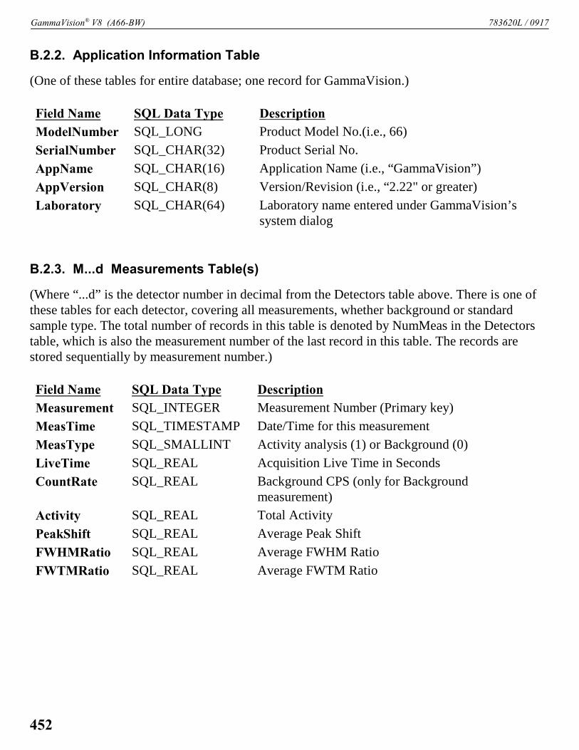
GammaVision® V8 (A66-BW) 783620L / 0917
B.2.2. Application Information Table
(One of these tables for entire database; one record for GammaVision.)
Field Name SQL Data Type Description
ModelNumber SQL_LONG Product Model No.(i.e., 66)
SerialNumber SQL_CHAR(32) Product Serial No.
AppName SQL_CHAR(16) Application Name (i.e., “GammaVision”)
AppVersion SQL_CHAR(8) Version/Revision (i.e., “2.22" or greater)
Laboratory SQL_CHAR(64) Laboratory name entered under GammaVision’ssystem dialog
B.2.3. M...d Measurements Table(s)
(Where “...d” is the detector number in decimal from the Detectors table above. There is one ofthese tables for each detector, covering all measurements, whether background or standardsample type. The total number of records in this table is denoted by NumMeas in the Detectorstable, which is also the measurement number of the last record in this table. The records arestored sequentially by measurement number.)
Field Name SQL Data Type Description
Measurement SQL_INTEGER Measurement Number (Primary key)
MeasTime SQL_TIMESTAMP Date/Time for this measurement
MeasType SQL_SMALLINT Activity analysis (1) or Background (0)
LiveTime SQL_REAL Acquisition Live Time in Seconds
CountRate SQL_REAL Background CPS (only for Backgroundmeasurement)
Activity SQL_REAL Total Activity
PeakShift SQL_REAL Average Peak Shift
FWHMRatio SQL_REAL Average FWHM Ratio
FWTMRatio SQL_REAL Average FWTM Ratio
452

783620L / 0917 APPENDIX B. FILE FORMATS
B.2.4. P...dmmmm Peaks Table(s)
(Where “...d” is the detector number in decimal, “mmmm” is the measurement number to 4places. There is one of these tables for each measurement in the table above, but only if theoutput of actual centroid energies is enabled.)
Field Name SQL Data Type Description
PeakNumber SQL_INTEGER Peak No. counter (Primary key)
PeakFlags SQL_INTEGER Analysis Results Flags
Nuclide SQL_CHAR(8) Library Nuclide Name this peak belongs to
Energy SQL_REAL Library Energy
Centroid SQL_REAL Actual Centroid Energy
CalFWHM SQL_REAL Expected (Calibrated) FWHM at this energy
FWHM SQL_REAL Actual FWHM
FWTM SQL_REAL Actual FWTM
Area SQL_REAL Net counts in peak
Background SQL_REAL Background counts
453

GammaVision® V8 (A66-BW) 783620L / 0917
[Intentionally blank]
454

APPENDIX C. ERROR MESSAGES
Errors are displayed in popup warning boxes, the lower-left corner of some MCB Propertiesdialogs, and the supplementary information line at the bottom of the window.
Acquisition Failure (JOB Error 11)For some reason an acquisition function failed from a .JOB file.
Already started.Detector already active when a Start Acquisition command was issued.
Altering Detector data.Restoring data to a Detector would destroy the data already there.
Amplifier not pole-zeroed.Warning from an MCB with automatic pole zero, indicating that the Detector should bepole-zeroed.
Analysis Completed for ...WAN32.EXE has finished executing.
Analysis Error <n>A call to DLAN1.DLL has been completed, but an error was encountered. The error code <n>has the following meaning:
Error # Warning # Reason
1 1 Read error in UFO peak record
1 2 Read error in UFO nuclide record
2 1 Write error in UFO peak record
2 2 Write error in UFO nuclide record
3 1 Invalid acquisition date and time
4 0 Illegal absorption correction
5 1 Read error in spectrum file
Analysis Failed!WAN32.EXE has finished executing, but an error was encountered. Refer to the “WAN32completion codes...” message.
Analysis Failed (Job Error 18)The ANALYZE command failed (look for the WAN32 error code for specifics).
455

GammaVision® V8 (A66-BW) 783620L / 0917
Analyzing (Please Wait) ...Analysis via DLAN1.DLL is being executed.
Attempt to dynamically link to a task! (WinExec error 5)Error encountered trying to spawn WAN32.EXE or some other application program.
Auto Calibration failed (Job Error 21)An error occurred when the CALIBRATE_AUTO command was executed.
Auto PZ aborted. The MCB Auto PZ function was aborted (by <Esc>).
Buffer and Detector not same size or segments.Error when trying to restore data that does not match the Detector configuration.
Calibration per channel wrong.Error when trying to calibrate spectrum, arising whenever the calibration slope would be 0,negative or greater than 100 units per channel.
Can’t allocate memory for library.Attempting to load a library for which there is not enough room in memory. Best dealtwith by trying again or removing some other applications from memory.
Can’t find any more peaks!A peak could not be found in the direction indicated by the function button pressed.
Can’t Find Any More ROIs.Attempting to index to the next ROI in a direction for which no more ROIs can be located.
Can’t read library file.Attempting to open or read the library file resulting in some kind of file I/O error, usuallybecause the file doesn’t exist, but also possibly because the disk is defective.
Can’t RESTORE to acquiring Detector.Error preventing the Restore function from altering data in a Detector in which one ormore segment(s) are actively acquiring data.
Can’t Run Protected Mode Application in Real Mode!(WinExec error 18)
Error encountered trying to spawn WAN32.EXE or some other application program.
456

783620L / 0917 APPENDIX C. ERROR MESSAGES
Can’t Run Second Instance of this .EXE (multiple writeable data segments)! (WinExecerror 16)
Error encountered trying to spawn WAN32.EXE or some other application program.
Can’t Run Second Instance of this .EXE (Non-shareable DLL in use)! (WinExec error 17)Error encountered trying to spawn WAN32.EXE or some other application program.
Cannot get valid Spectral Data!The File/Save function was not presented with valid spectral data; usually the result ofproblems obtaining data from a Detector.
Comm. Failure!Detector communication failure, most likely resulting from a timeout (the Detector failedto respond within a reasonable period of time).
Configuration failed!Attempted reconfiguration failed, most likely because of some conflict with Detectorsphysically installed.
Could not properly fit the peak.Function requiring a fitted peak could not obtain an acceptable peak, probably because oftoo few counts, too narrow, or non-Gaussian peak shape, or bad statistics such ascalculated sigma-squared less than zero.
Couldn’t get background subtracted ROI.A function requiring a background subtracted ROI couldn’t obtain such, probably becausethere was no ROI at the point specified, or maybe because there weren’t statisticallysignificant counts above background.
Default Printer Failed! Undefined at Control Panel?The REPORT or PRINT function was aborted because the default system printer has notbeen properly set up. Go to the Printers function in Windows Control Panel, install theappropriate printer, and select it as outlined in the Microsoft Windows documentation.
Detector #.. ; ......... ; Error ... (Macro) ... (Micro)An unresolved error originating in the Detector. The offending Detector command isshown, together with the macro and micro error codes. If the error persists, the error codesshould be recorded and the factory should be contacted. These error codes are explained inthe hardware manual for the Detector.
457

GammaVision® V8 (A66-BW) 783620L / 0917
Detector busy or Segment not responding.This indicates the Detector was unable to respond within a certain time limit, due to otheractivities, such as multiple instances of GammaVision accessing the Detector at the sametime, or otherwise heavy use of the Detector interface.
Detector does not support Field Mode (Job Error 19)An attempt was made to execute the LOOP_SPECTRA or VIEW command on a Detectorthat does not support Field Mode.
Detector Error!The selected Detector could not be STARTed or STOPped due to some unresolved errorcondition.
Detector Not Located.A Detector could not be located at the configured address.
Do you want to save buffer?A function that would destroy the buffer (such as COPY or EXIT) queries the user unlessthe buffer has not been modified since last being saved.
Do you want to save Library?The nuclide library has been modified by the library editor, but the user has not yet savedthe changes.
DOS 4.0 Application! (WinExec error 13)Error encountered trying to spawn WAN32.EXE or some other application program.
Error opening file.If trying to write a file, this would indicate a disk controller problem such as a full disk. Iftrying to read a file, this would indicate that the filename specified could not be found.
Error reading file -- STRIP aborted.Could not read the file requested for stripping.
Error reading file.File read error is usually a result of damaged media.
Error writing file.File write error is usually a result of damaged media or full disk.
458

783620L / 0917 APPENDIX C. ERROR MESSAGES
.EXE for earlier version of Windows! (WinExec error 15)Error encountered trying to spawn WAN32.EXE or some other application program.
Failure obtaining ROI (or Peak).A function that requires a defined ROI (or Peak, in the case of the Calibrate function)when the marker is not placed in a channel with an ROI bit set (and if a Peak is not veryclose by).
Failure of Detector function (JOB Error 12)This error arises from a JOB that encounters an error when trying to access a Detector.
File already exists!If the file output function requested would write a file with the same name as another filethat already exists, the user is prompted for confirmation of the operation by this warning.See also “OK To Overwrite Existing File?”
File is wrong size Can’t STRIP.The STRIP function requires a compatible file for stripping from the spectrum in memory;i.e., must contain the same number of channels.
File Not Found! (WinExec error 2)Error encountered trying to spawn WAN32.EXE or some other application program.
Fine gain is at limit of ...This message appears in the Information Line when an attempt is made to change the MCBgain setting with the keyboard function, but while the MCB cannot be decreased orincreased any further.
FWHM Fit Error Exceeds 25%.The peaks entered in an energy calibration produced a FWHM fit with an error on at leastone peak greater than 25%.
Hardware failure!This message appears as the result of a Detector execution error with micro code 137,indicating a hardware failure.
High voltage not enabled.START was attempted on a 92X while the high voltage was not enabled.
Illegal Entry!Certain values are not permitted in manual dialog entries or tables.
459
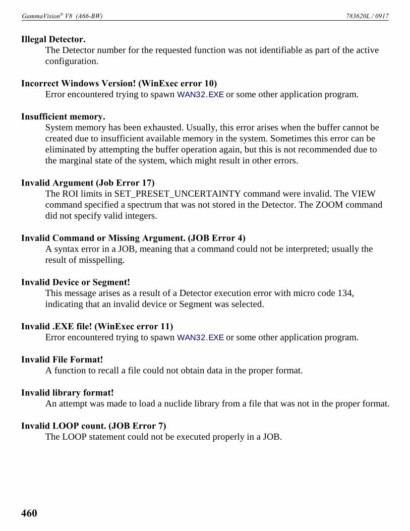
GammaVision® V8 (A66-BW) 783620L / 0917
Illegal Detector.The Detector number for the requested function was not identifiable as part of the activeconfiguration.
Incorrect Windows Version! (WinExec error 10)Error encountered trying to spawn WAN32.EXE or some other application program.
Insufficient memory.System memory has been exhausted. Usually, this error arises when the buffer cannot becreated due to insufficient available memory in the system. Sometimes this error can beeliminated by attempting the buffer operation again, but this is not recommended due tothe marginal state of the system, which might result in other errors.
Invalid Argument (Job Error 17)The ROI limits in SET_PRESET_UNCERTAINTY command were invalid. The VIEWcommand specified a spectrum that was not stored in the Detector. The ZOOM commanddid not specify valid integers.
Invalid Command or Missing Argument. (JOB Error 4)A syntax error in a JOB, meaning that a command could not be interpreted; usually theresult of misspelling.
Invalid Device or Segment!This message arises as a result of a Detector execution error with micro code 134,indicating that an invalid device or Segment was selected.
Invalid .EXE file! (WinExec error 11)Error encountered trying to spawn WAN32.EXE or some other application program.
Invalid File Format!A function to recall a file could not obtain data in the proper format.
Invalid library format!An attempt was made to load a nuclide library from a file that was not in the proper format.
Invalid LOOP count. (JOB Error 7)The LOOP statement could not be executed properly in a JOB.
460

783620L / 0917 APPENDIX C. ERROR MESSAGES
Invalid Start Date/Time -- Battery Backup Lost??A 919 or 92X Detector contained an unrecognizable start date. This is usually anindication that the backup power was lost.
Invalid Start Record.No valid Start Record file could be found to provide the start date/time for an installed 917or 918 Detector.
JOB Aborted or Premature EOF (JOB Error 1)A JOB was aborted by the user, or an End-of-File was encountered while trying to obtain acommand from the executing .JOB file.
JOB Error.A generic error message indicating that an error was encountered while executing a .JOB
file. Usually some explanatory phrase is given.
Library requires separate data segments for each task!(WinExec error 6)
Error encountered trying to spawn WAN32.EXE or some other application program.
Library too large to load.Library files larger than 65,000 bytes are not admissible as internally resident libraries.(However, any size library can be used for Master Library.)
Multiple-device Detector added.While performing the CONFIGURATION dialog function ADD, a 919 device type wasspecified, and there is room to add up to four Detectors for each 919 device added; theADD function is automatically repeated for each possible Detector number.
Must have a value greater than zero!Certain analysis or library table entries require values greater than 0.0.
Must have valid calibration!Certain analysis functions cannot be performed if the calibration is invalid.
Must select 92X type Detector!This error results from an attempt to perform a function available for only 92X-typeDetectors.
Need an ROI at the desired peak location.The Stabilizer function requires a valid ROI at the desired peak.
461

GammaVision® V8 (A66-BW) 783620L / 0917
No Buffer to RESTORE from!The RESTORE function requires a valid spectrum in buffer.
No close library match.The REPORT function could not obtain a library entry close enough to the located peak.
No File Name.A file function was requested without specifying the filename adequately.
No more library peak energies!A peak search was attempted in a direction where no more can be found.
No more multiplets!The multiplet finding sidebar function in Analysis Results display mode cannot find anymore multiplets in the direction indicated.
No more peaks for this nuclide!The “peaks within nuclide” sidebar function in Analysis Results mode cannot find anymore peaks within the selected nuclide.
No more unknown peaks!The unknown peak finding sidebar function in Analysis Results display mode cannot findany more unknown peaks in the direction indicated.
No peaks found!The peak search function could not find any valid peaks in the spectrum.
No ROI found to report!The REPORT function could not find any ROIs in range.
No ROI There To Clear.The Clear ROI function (the <Del> or <Delete> key) requires at least one channel at themarker with the ROI bit set.
No segment selected.The Detector function could not be performed because no Segment was selected.
Not Allowed During Acquisition!An execution error (micro 135) arising from the Detector, indicating that the Detectorcommand is not allowed while acquisition is in progress.
462

783620L / 0917 APPENDIX C. ERROR MESSAGES
Not Allowed During Current Mode!An execution error arising from the Detector (micro 136), indicating that the Detectorcommand attempted is not allowed in the current mode of operation.
Not enough data points for fit.Efficiency calibration fit for specified type requires a minimum number of table entries forthat type; e.g., for a polynomial fit, six or more points are required.
Not enough memory STRIP aborted.The STRIP function temporarily allocates enough memory to read the file, but theallocation failed in this case, probably due to insufficient available memory in the system.The STRIP function is discontinued.
Not enough memory for COMPARE.The COMPARE mode could not be executed due to insufficient memory for the secondspectrum.
NOTE: Settings for SEGMENT <n>GammaVision is informing the user in the case of multi-segment Detector that he isperforming settings (e.g., through an ASK function) on a specific segment only.
OK to add another device?When a 919 device is being added in the CONFIGURATION dialog, the user is promptedfor confirmation before automatically proceeding with the addition of up to four Detectornumbers.
OK to attempt another instance?Attempt to start an analysis (via WAN32.EXE) while a previous analysis has not yetfinished, or had been aborted abnormally. GammaVision is asking the user to allow it tocontinue with this operation in case it is not properly sensing the state of the previousanalysis. If the user permits this to continue (by answering Yes), but if the previousinstance was actually still running, then another “WinExec()...” error will occur.
OK to destroy contents of Detector?The RESTORE function prompts the user for confirmation before writing the contents ofthe buffer into the Detector.
OK to overwrite ‘...’ ?A file output function discovered that the specified filename already exists, and will onlyoverwrite the file after the user confirms his intentions. See also “File already exists!”
463

GammaVision® V8 (A66-BW) 783620L / 0917
OK to save changes?The user is being prompted to allow the system to save a modified file such as a libraryfile, table file, or sample-type defaults file.
OK to use it anyway?A new configuration was applied but failed due to some conflict with the Detectorsphysically present; it is possible to use the configuration anyway by answering Yes to thisquery.
OS/2 Application! (WinExec error 12)Error encountered trying to spawn WAN32.EXE or some other application program.
Out of Memory! (WinExec error 0 )Error encountered trying to spawn WAN32.EXE or some other application program.
Path Not Found! (WinExec error 3)Error encountered trying to spawn WAN32.EXE or some other application program.
Peak rejected for asymmetry.Peak statistics could not be obtained for the function due the calculated non-Gaussianasymmetry of the obtained peak.
Preset already reached.Acquisition START was attempted on a Detector or Segment that had already satisfied thepreset condition(s) in some way.
Presets can’t be changed during acquisition.Changes in the preset condition(s) are not allowed while the Detector is actively acquiring.
Presets not programmed to Detector correctly!Usually a failure of the selected Detector to accept the commands from GammaVision toprogram presets. Often the result of improper configuration or faulty interface.
Previous analysis did not run to completion!Attempt to start an analysis (via WAN32.EXE) while a previous analysis has not yetfinished, or had been aborted abnormally. See “OK to attempt another instance?”
Problem with Buffer. (JOB Error 2)A JOB error resulting from some problem with the buffer, usually indicating insufficientmemory to create or enlarge the buffer as needed.
464

783620L / 0917 APPENDIX C. ERROR MESSAGES
Problem with Calculation. (JOB Error 13)A JOB error resulting from a problem with a calculation.
Problem with RECALL. (JOB Error 10)The RECALL statement could not be executed in a JOB.
Problem with REPORT. (JOB Error 14)The REPORT function could not be exercised in a JOB.
Problem with SAVE. (JOB Error 9)The SAVE function could not be executed in a JOB.
QA failed (Job Error 22)An error occurred when the QASAMPLE or QABACKGROUND command was executed.
Sample Changer Hardware Failure. (JOB Error 16)The Sample Changer hardware handshake failed in some way; usually the result of toomuch time before SAMPLE READY is obtained.
Start/Save/Report sequence aborted!Start/Save/Report sequence aborted (usually by manual intervention, but also resultingfrom certain errors.)
Start/Save/Report waiting for completion of previous analysis...A status message indicating that the Start/Save/Report sequence has been suspendedwhile waiting for completion of an ongoing analysis.
Table is Full!A limit of 96 entries is allowed in the calibration table.
There are no stored spectra to view (Job Error 20)An attempt was made to execute the LOOP_SPECTRA or VIEW command on a Detectorthat does not have any stored spectra.
The Serial I/O Command timed out (Job Error 24)The WAIT_SERIAL command timed out before receiving a response from the selectedDetector.
The Serial I/O Response did not match (Job Error 25)The WAIT_SERIAL command did not time out, however, the actual and expectedresponses did not match.
465

GammaVision® V8 (A66-BW) 783620L / 0917
The WAIT program was not started by GammaVision (Job Error 23)All programs “WAITed for” have to be started by GammaVision.
Token Error.A token error in a JOB, meaning that some argument to the command was invalid or out ofcontext.
Unable to CALL -- Invalid file name. (JOB Error 8)A JOB error resulting from a problem with the CALL function (usually because the filedoes not exist).
Unable to COMPARE files of different sizes.The COMPARE function requires compatible files.
Unable to cut peak or peak not selected!The library editor Cut function or Analysis Results Delete library peak function iscomplaining that it cannot cut or delete a peak from the library for some reason, usuallybecause a peak is not selected.
Unable to open file -- STRIP aborted.The STRIP function is aborted if the file cannot be read.
Unable to open file for COMPARE.The COMPARE function is aborted if the second spectrum cannot be read.
Unable to Read Specified File. (JOB Error 3)A file input/output error encountered while executing a JOB.
Unable to RUN non-executable program. (JOB Error 6)The specified program could not be RUN from a JOB.
Unable to strip Detector memory.The stripping function must be performed in the buffer.
Unknown .EXE type! (WinExec error 14)Error encountered trying to spawn WAN32.EXE or some other application program.
Unknown (misspelled) Command. (JOB Error 5)A command in a .JOB file could not be executed because it could not be interpreted as avalid command (usually a result of misspelling).
466

783620L / 0917 APPENDIX C. ERROR MESSAGES
WAIT program was not started by GammaVision (JOB Error 23)All programs “WAITed for” have to be started by GammaVision. In 32-bit Windows, the32-bit programs are completely independent.
WAN32 completion codes: i=<i> errnum=<e> warnum=<w>The following numbers are returned by the analysis routines and displayed on theinformation line.
Error # Warning # Reason 1 ? Invalid spectrum filename 1 1 Read error in UFO peak record 1 2 Read error in UFO nuclide record 1 3 Read error in spectrum non-data record 1 4 Read error in UFO file 1 200 Attempt to read start channel after stop channel 1 201 Read error on disk for .CHN files 1 202 Read error on disk for .SPC files 1 203 Attempt to read invalid spectrum file type 2 0 Illegal filename 2 1 Write error in UFO peak record 2 2 Write error in UFO nuclide record 2 3 Write error in other UFO records 2 4 Invalid record for UFO file 2 7 Write error on report file 2 8 Invalid record request for table file 3 0 Invalid acquisition date and time 4 0 Illegal absorption correction 4 3 Spectrum not found 5 0 Read error in spectrum file 5 3 Spectrum wrong file type 6 1 Library not sorted 6 2 Read error on library 6 3 Invalid record request for library 6 4 Library not found 10 Error # System error (e.g., math overflow)
Warning 128.Warning 64.Warning 8.
All three of the above messages are the result of Detector Start or Stop warnings and arehardware dependent.
467
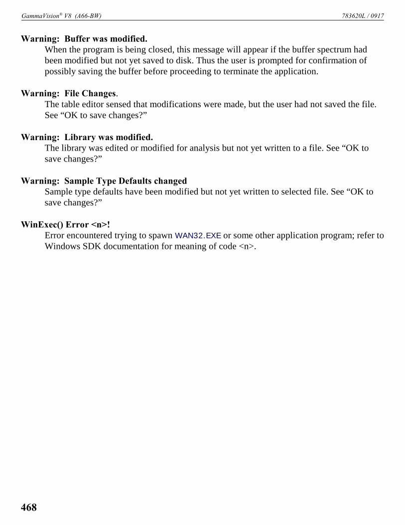
GammaVision® V8 (A66-BW) 783620L / 0917
Warning: Buffer was modified.When the program is being closed, this message will appear if the buffer spectrum hadbeen modified but not yet saved to disk. Thus the user is prompted for confirmation ofpossibly saving the buffer before proceeding to terminate the application.
Warning: File Changes.The table editor sensed that modifications were made, but the user had not saved the file.See “OK to save changes?”
Warning: Library was modified.The library was edited or modified for analysis but not yet written to a file. See “OK tosave changes?”
Warning: Sample Type Defaults changedSample type defaults have been modified but not yet written to selected file. See “OK tosave changes?”
WinExec() Error <n>!Error encountered trying to spawn WAN32.EXE or some other application program; refer toWindows SDK documentation for meaning of code <n>.
468

INDEX
.AN1.. . . . . . . . . . . . . . . . . . . . . . . . . . . . . . 52, 449
.ATT.. . . . . . . . . . . . . . . . . . . . . . . . . . . . . 172, 450
.CFG.. . . . . . . . . . . . . . . . . . . . . . . . . . . . . . . . 449
.CHN. . . . . . . . . . . . . . . . . . . . . . . . . . 57, 103, 449
.CLB.. . . . . . . . . . . . . . 32, 129, 130, 268, 401, 449
.CXT.. . . . . . . . . . . . . . . . . . . . . . . . . . . . . . . . 449
.DAC. . . . . . . . . . . . . . . . . . . . . . . . . . . . . . . . 450
.EBR.. . . . . . . . . . . . . . . . . . . . . . . . . . . . . 308, 450
.EFT. . . . . . . . . . . . . . . . . . . . . . . . . . . . . . 125, 450
.ENT.. . . . . . . . . . . . . . . . . . . . . . . . . . 29, 111, 450
.GEO. . . . . . . . . . . . . . . . . . . . . . . . . . . . . 173, 450
.IEQ. . . . . . . . . . . . . . . . . . . . . . . . . . . . . . . . . 450
.JOB (see also Job). . . . . . . . . . . . . . . . . . . 381, 450
.LIB. . . . . . . . . . . . . . . . . . . . . . . . . . . 52, 206, 449
.LIS.. . . . . . . . . . . . . . . . . . . . . . . . . . . . . . . . . . . 6
.MDB. . . . . . . . . . . . . . . . . . . . . . . . . . . . . . . . 450
.PBC. . . . . . . . . . . . . . . . . . . . . . . . . . . . . . . . . 174
.ROI. . . . . . . . . . . . . . . . . . . . . . . . . . . . . . . . . 449
.RPT. . . . . . . . . . . . . . . . . . . . . . . . . . . . . . 158, 450
.SDF. . . . . . . . . . . . . . . . . . . . . . . . . . . . . . . . . 449
.SPC. . . . . . . . . . . . . . . . . . . . . . . . . . 103, 129, 449floating-point. . . . . . . . . . . . . . . . . . . . . . . . . 57integer. . . . . . . . . . . . . . . . . . . . . . . . . . . . . . 57
.SPE. . . . . . . . . . . . . . . . . . . . . . . . . . . . . . . . . . 57
.TXT.. . . . . . . . . . . . . . . . . . . . . . . . . . . . . . . . 450
.UFO.. . . . . . . . . . . . . . . . . . . . . . . . . . . . . . . . 449??? (Job loop counter). . . . . . . . . . . . . . . . . . . . 398Absorption. . . . . . . . . . . . . . . . . . . . . . . . . . . . 286
example ratio. . . . . . . . . . . . . . . . . . . . . . . . 288example table.. . . . . . . . . . . . . . . . . . . . . . . 290external. . . . . . . . . . . . . . . . . . . . . . . . . . . . 286internal. . . . . . . . . . . . . . . . . . . . . . . . . . . . 287
Accelerator keys. . . . . . . . . . . . . . . . . . . . . . . . 371keyboard map. . . . . . . . . . . . . . . . . . . . . . . 373quick-reference table. . . . . . . . . . . . . . . . . . 372
Acceptance thresholds, QA. . . . . . . . . . . . . . . . 360Acquire menu. . . . . . . . . . . . . . . . . . . . . . . . . . . 70Acquisition presets. . . . . . . . . . . . . . . . . . . . . . . 87
ask on start.. . . . . . . . . . . . . . . . . . . . . . . . . . 72Acquisition settings. . . . . . . . . . . . . . . . . . . . . . . 70Amplifier gain
fine. . . . . . . . . . . . . . . . . . . . . . . . . . . . . . . 376Analog-to-Digital Converter (ADC). . . . . . . . . . . 4
Analysisanalysis engine setup. . . . . . . . . . . . . . . . . . 436analysis engines. . . . . . . . . . . . . . . . . . . . . . 435display results. . . . . . . . . . . . . . . . . . . . . . . . 194energy recalibration. . . . . . . . . . . . . . . . . . . 251ENV32 engine. . . . . . . . . . . . . . . . . . . . . . . 232GAM32 engine.. . . . . . . . . . . . . . . . . . . 160, 232interactive.. . . . . . . . . . . . . . . . . . . . . . . . . . 203manual peak stripping.. . . . . . . . . . . . . . 160, 265NPP32 engine.. . . . . . . . . . . . . . . . . . . . 161, 232peak details.. . . . . . . . . . . . . . . . . . . . . . . . . 202peak search.. . . . . . . . . . . . . . . . . . . . . . . . . 254residuals. . . . . . . . . . . . . . . . . . . . . . . . . . . . 196ROI32 engine. . . . . . . . . . . . . . . . . . . . . . . . 233spectrum on disk.. . . . . . . . . . . . . . . . . . . . . 193spectrum on display. . . . . . . . . . . . . . . . . . . 193WAN32 engine. . . . . . . . . . . . . . . . . . . 160, 231
Analysis results spectrum menu. . . . . . . . . . . . . 196Analyze menu. . . . . . . . . . . . . . . . . . . . . . . . . . 149Arguments
import.. . . . . . . . . . . . . . . . . . . . . . . . . . . . . . 61Ask on Save.. . . . . . . . . . . . . . . . . . . . . . . . . . . 382Ask on Start. . . . . . . . . . . . . . . . . . . . . . . . . . 71, 382
acquisition presets. . . . . . . . . . . . . . . . . . . . . 72collection date and time. . . . . . . . . . . . . . . . . 72sample description. . . . . . . . . . . . . . . . . . . . . 72sample quantity.. . . . . . . . . . . . . . . . . . . . . . . 72sample type defaults. . . . . . . . . . . . . . . . . . . . 72
Associated files. . . . . . . . . . . . . . . . . . . . . . . . . . 52Attenuation
automatic. . . . . . . . . . . . . . . . . . . . . . . . . . . 171calculate. . . . . . . . . . . . . . . . . . . . . . . . . . . . 171coefficients. . . . . . . . . . . . . . . . . . . . . . . . . . 166external.. . . . . . . . . . . . . . . . . . . . . . . . . . . . 163internal. . . . . . . . . . . . . . . . . . . . . . . . . . . . . 163manual. . . . . . . . . . . . . . . . . . . . . . . . . . . . . 171
Auto-clear ROI. . . . . . . . . . . . . . . . . . . . . . . . . 222Average energy. . . . . . . . . . . . . . . . . . . . . . 164, 308
table. . . . . . . . . . . . . . . . . . . . . . . . . . . . . . . 180B30WINDS.INI. . . . . . . . . . . . . . . . . . . . . . . . . 436
ISO NORM flags. . . . . . . . . . . . . . . . . . . . . 444Background
example. . . . . . . . . . . . . . . . . . . . . . . . . . . . 241
469

GammaVision® V8 (A66-BW) 783620L / 0917
for multiplets. . . . . . . . . . . . . . . . . . . . . . . . . 259parabolic. . . . . . . . . . . . . . . . . . . . . . . . . . . 262stepped. . . . . . . . . . . . . . . . . . . . . . . . . . . . 261
Background methods. . . . . . . . . . . . . . . . . . . . . 238Branching ratio. . . . . . . . . . . . . . . . . . . . . . . . . . 266buffer. . . . . . . . . . . . . . . . . . . . . . . . . . . . 4, 74, 229
Detector and buffer concept.. . . . . . . . . . . . . . 17Calculate menu. . . . . . . . . . . . . . . . . . . . . . . . . . 143Calibrate menu. . . . . . . . . . . . . . . . . . . . . . . . . . 103Calibration. . . . . . . . . . . . . . . . . . . . . . . . . . . . 103
Automatic. . . . . . . . . . . . . . . . . . . . . . . . . . 123automatic, efficiency. . . . . . . . . . . . . . . . . . . 125automatic, energy.. . . . . . . . . . . . . . . . . 106, 396certificate.. . . . . . . . . . . . . . . . . . . . . . . . 30, 120efficiency.. . . . 30, 104, 114, 115, 123, 396, 401energy. . . . . . . . . . . 26, 104, 105, 206, 396, 401internal. . . . . . . . . . . . . . . . . . . . . . . . . . . . 151manual, efficiency. . . . . . . . . . . . . . . . . . . . . 125manual, energy. . . . . . . . . . . . . . . . . . . . . . . 107peak shape. . . . . . . . . . . . . . . . . . . . . . . . . . . 105print. . . . . . . . . . . . . . . . . . . . . . . . . . . . . . . 130recalibration.. . . . . . . . . . . . . . . . . . . . . 111, 115recall. . . . . . . . . . . . . . . . . . . . . . . . . . . . . . 129save. . . . . . . . . . . . . . . . . . . . . . . . . . . . . . . 130working. . . . . . . . . . . . . . . . . . . . . . . . . 129, 151
Calibration Wizard. . . . . . . . . . . . . . . . . . . 103, 132efficiency calibration. . . . . . . . . . . . . . . . . . . 135energy calibration. . . . . . . . . . . . . . . . . . . . . 133TCC calibration. . . . . . . . . . . . . . . . . . . . . . . 135
Center. . . . . . . . . . . . . . . . . . . . . . . . . . . . . . 48, 225Clear ROI. . . . . . . . . . . . . . . . . . . . . . . 47, 222, 230Clear spectrum. . . . . . . . . . . . . . . . . . . . 47, 74, 397Collection date and time. . . . . . . . . . . . . . . . . . . . 58
ask on start. . . . . . . . . . . . . . . . . . . . . . . . . . . 72Command line
GammaVision. . . . . . . . . . . . . . . . . . . . . . . 433GVPlot. . . . . . . . . . . . . . . . . . . . . . . . . . . . 431MCB Configuration.. . . . . . . . . . . . . . . . . . . 14TRANSLT.. . . . . . . . . . . . . . . . . . . . . . . . . 431
Compare spectra. . . . . . . . . . . . . . . . . . 66, 227, 372Configuration
analysis setup.. . . . . . . . . . . . . . . . . . . . . . . . 435Copy to buffer.. . . . . . . . . . . . . . . . . . . . . . . . . . . 74Correction. . . . . . . . . . . . . . . . . . . . . . . . . . . . . 162
attenuation. . . . . . . . . . . . . . . . . . . . . . . . . . 163
geometry. . . . . . . . . . . . . . . . . . . . . . . . 163, 173isotope-specific corrections.. . . . . . . . . . . . . 164random summing. . . . . . . . . . . . . . . . . . . . . 293
DAC. . . . . . . . . . . . . . . . . . . . . . . . . . . . . . . . . 165table. . . . . . . . . . . . . . . . . . . . . . . . . . . . . . . 184
decay correction. . . . . . . . . . . . . . . . . . . 58, 155, 281deconvolution. . . . . . . . . . . . . . . . . . . . . . . . . . 104Derived Activity Calculation - see DAC. . . . . . . 165detector
background, QA. . . . . . . . . . . . . . . . . . . . . . 355database, QA. . . . . . . . . . . . . . . . . . . . . . . . 355Detector and buffer concept. . . . . . . . . . . . . . . 17detector table, QA. . . . . . . . . . . . . . . . . . . . . 450list. . . . . . . . . . . . . . . . . . . . . . . . . . . . . . . . 434lock. . . . . . . . . . . . . . . . . . . . . . . . . . . . . . . 218lock/unlock (password).. . . . . . . . . . . . . . . . . . 5pick list.. . . . . . . . . . . . . . . . . . . . . . . . . . . 43, 49status sidebar. . . . . . . . . . . . . . . . . . . . . . . . . 45unlock. . . . . . . . . . . . . . . . . . . . . . . . . . . . . 218
Detector list. . . . . . . . . . . . . . . . . . . . . . . . . . . . . 43Directed fit.. . . . . . . . . . . . . . . . . . . . . . . . . 161, 244Directories
GammaVision file locations. . . . . . . . . . . . . . 62Display
mode (points/fill). . . . . . . . . . . . . . . . . . . . . 227spectrum colors. . . . . . . . . . . . . . . . . . . . . . 227
Display menu.. . . . . . . . . . . . . . . . . . . . . . . . . . 223Dose Equivalent Iodine - see Iodine equivalence. 310Drag and drop. . . . . . . . . . . . . . . . . . . . . . . . . . . 52DSPEC-50
ADC setup. . . . . . . . . . . . . . . . . . . . . . . . . . . 83amplifier settings. . . . . . . . . . . . . . . . . . . . 77, 79anticoincidence.. . . . . . . . . . . . . . . . . . . . . . . 83coincidence.. . . . . . . . . . . . . . . . . . . . . . . . . . 83Enhanced throughput mode. . . . . . . . . . . . . . 81high-voltage setup. . . . . . . . . . . . . . . . . . . . . 85live-time preset. . . . . . . . . . . . . . . . . . . . . . . . 88low-frequency rejector (LFR). . . . . . . . . . . . . 80lower level discriminator. . . . . . . . . . . . . . . . 84MDA preset. . . . . . . . . . . . . . . . . . . . . . . . . . 89noise rejection level. . . . . . . . . . . . . . . . . . . . 81Nuclide Report setup tab. . . . . . . . . . . . . . . . . 90optimize. . . . . . . . . . . . . . . . . . . . . . . . . . . . . 78real-time preset. . . . . . . . . . . . . . . . . . . . . . . . 88Resolution Enhancer.. . . . . . . . . . . . . . . . . . . 82
470

INDEX
ROI integral preset.. . . . . . . . . . . . . . . . . . . . . 88ROI peak count preset. . . . . . . . . . . . . . . . . . . 88stabilizer setup. . . . . . . . . . . . . . . . . . . . . . . . 84zero dead-time (ZDT) mode. . . . . . . . . . . . . . 84
EBAR - see Average energy. . . . . . . . . . . . . . . . 308Efficiency calibration. . . . . . . . . . . . . . . . . 103, 114
automatic from .EFT file. . . . . . . . . . . . . . . . 125Calibration Wizard.. . . . . . . . . . . . . . . . 132, 135interpolative.. . . . . . . . . . . . . . . . . . . . . . . . 117knee energy. . . . . . . . . . . . . . . . . . . . . . . . . . 122linear. . . . . . . . . . . . . . . . . . . . . . . . . . . . . . 118manual.. . . . . . . . . . . . . . . . . . . . . . . . . . . . 125performing.. . . . . . . . . . . . . . . . . . . . . . . . . 120polynomial.. . . . . . . . . . . . . . . . . . . . . . . . . 119quadratic. . . . . . . . . . . . . . . . . . . . . . . . . . . 118recall. . . . . . . . . . . . . . . . . . . . . . . . . . . . . . 129standards file (.EFT). . . . . . . . . . . . . . . . . . . 125TCC polynomial fit. . . . . . . . . . . . . . . . . . . . 120using a library. . . . . . . . . . . . . . . . . . . . . . . . 123working library. . . . . . . . . . . . . . . . . . . . . . . 120
Energy calibration. . . . . . . . . . . . . . . . . . . . 103, 105Auto Calibrate. . . . . . . . . . . . . . . . . . . . . . . . 106Calibration Wizard.. . . . . . . . . . . . . . . . 132, 133manual.. . . . . . . . . . . . . . . . . . . . . . . . . . . . 107recalibration.. . . . . . . . . . . . . . . . . . . . . . . . 111recall. . . . . . . . . . . . . . . . . . . . . . . . . . . . . . 129standards file (.ENT). . . . . . . . . . . . . . . . . . . 109using a library. . . . . . . . . . . . . . . . . . . . . . . . 112using multiple spectra. . . . . . . . . . . . . . . . . . 113
Energy-normalized difference. . . . . . . . . . . . . . . 253ENV32 analysis engine. . . . . . . . . . . . . . . . . . . . 232Error messages. . . . . . . . . . . . . . . . . . . . . . . . . . 455Exit. . . . . . . . . . . . . . . . . . . . . . . . . . . . . . . . . . . 69Expanded Spectrum View.. . . . . . . . . . . . . . . 45, 46Export
file. . . . . . . . . . . . . . . . . . . . . . . . . . . . . . . . . 58setup. . . . . . . . . . . . . . . . . . . . . . . . . . . . . . . 59spectrum. . . . . . . . . . . . . . . . . . . . . . . . . . . . 65
External Absorption. . . . . . . . . . . . . . . . . . . . . . 286File
export. . . . . . . . . . . . . . . . . . . . . . . . . . . . . . 58GammaVision file locations.. . . . . . . . . . . . . . 62import. . . . . . . . . . . . . . . . . . . . . . . . . . . . . . 61recall spectrum.. . . . . . . . . . . . . . . . . . . . . . . 63save spectrum. . . . . . . . . . . . . . . . . . . . . . . . 64
File settings. . . . . . . . . . . . . . . . . . . . . . . . . . . . . 56collection date and time. . . . . . . . . . . . . . . . . . 58sample description. . . . . . . . . . . . . . . . . . . . . 58sample quantity. . . . . . . . . . . . . . . . . . . . . . . 58
files, GV sample. . . . . . . . . . . . . . . . . . . . . . . . . 17Fine gain. . . . . . . . . . . . . . . . . . . . . . . . . . . . . . 376Fraction limit. . . . . . . . . . . . . . . . . . . . . . . . 153, 266Full Spectrum View. . . . . . . . . . . . . . . . . . . . . 45, 46
sizing and moving. . . . . . . . . . . . . . . . . . . . . 50FW(1/x)M. . . . . . . . . . . . . . . . . . . . . . . . . . . . . 143FW1/xM. . . . . . . . . . . . . . . . . . . . . . . . . . . . . . 144FWHM. . . . . . . . . . . . . . . . . . . . . . . . . . . . . 29, 144Gain
fine.. . . . . . . . . . . . . . . . . . . . . . . . . . . . . . . 376Gain stabilization. . . . . . . . . . . . . . . . . . . . . . . . . 84
Initialize. . . . . . . . . . . . . . . . . . . . . . . . . . . . . 84Gain stabilizer
operation details. . . . . . . . . . . . . . . . . . . . . . . 93GAM32 analysis engine.. . . . . . . . . . . . . . . 160, 232Gamma Total (EDF). . . . . . . . . . . . . . . . . . . . 2, 186
analysis methods.. . . . . . . . . . . . . . . . . . . . . 324filename conventions. . . . . . . . . . . . . . . . . . 188generating the Gamma Total reports.. . . . . . . 189hardware and analysis setup. . . . . . . . . . . . . . 188report table in GammaVision report. . . . . . . . 352
Geometry correction.. . . . . . . . . . . . . . 163, 173, 284automatic. . . . . . . . . . . . . . . . . . . . . . . . . . . 173example. . . . . . . . . . . . . . . . . . . . . . . . . . . . 285manual. . . . . . . . . . . . . . . . . . . . . . . . . . . . . 173
GVPlot.. . . . . . . . . . . . . . . . . . . . . . . . . . . . . . . 419command line interface. . . . . . . . . . . . . . . . . 431
Horizontal Scale.. . . . . . . . . . . . . . . . . . . . . . . . 379Center.. . . . . . . . . . . . . . . . . . . . . . . . . . . . . . 48Zoom In. . . . . . . . . . . . . . . . . . . . . . . . . . . . . 48Zoom Out.. . . . . . . . . . . . . . . . . . . . . . . . . . . 48
Importarguments.. . . . . . . . . . . . . . . . . . . . . . . . . . . 61file. . . . . . . . . . . . . . . . . . . . . . . . . . . . . . . . . 61setup.. . . . . . . . . . . . . . . . . . . . . . . . . . . . . . . 61spectrum file.. . . . . . . . . . . . . . . . . . . . . . . . . 65
Indexing buttons. . . . . . . . . . . . . . . . . . . . . . . . . 51LIB.. . . . . . . . . . . . . . . . . . . . . . . . . . . . . 51, 374PEAK.. . . . . . . . . . . . . . . . . . . . . . . . . . . 51, 374ROI. . . . . . . . . . . . . . . . . . . . . . . . . . . . . 52, 374
InSight Mode. . . . . . . . . . . . . . . . . . . . . . . . . . 79, 80
471

GammaVision® V8 (A66-BW) 783620L / 0917
Mark. . . . . . . . . . . . . . . . . . . . . . . . . . . . . . 100Mark types.. . . . . . . . . . . . . . . . . . . . . . . . . . 100
Installation. . . . . . . . . . . . . . . . . . . . . . . . . . . . . . 7installing Connections. . . . . . . . . . . . . . . . . . . 7installing GammaVision. . . . . . . . . . . . . . . . . 7registration.. . . . . . . . . . . . . . . . . . . . . . . . . . 15running MCB Configuration. . . . . . . . . . . . . . 9
Internal Absorption. . . . . . . . . . . . . . . . . . . . . . . 287Iodine equivalence. . . . . . . . . . . . . . . 164, 183, 310
table.. . . . . . . . . . . . . . . . . . . . . . . . . . . . . . 183Iodine Equivalence Table. . . . . . . . . . . . . . . . . . 183ISO NORM
analysis methods. . . . . . . . . . . . . . . . . . . . . . 313report setup. . . . . . . . . . . . . . . . . . . . . . . . . . 157
Jobcommand catalog.. . . . . . . . . . . . . . . . . . . . . 390control. . . . . . . . . . . . . . . . . . . . . . . . . . . . . 215edit. . . . . . . . . . . . . . . . . . . . . . . . . . . . . . . 215example. . . . . . . . . . . . . . . . . . . . . . . . . . . . 385file. . . . . . . . . . . . . . . . . . . . . . . . . . . . . . . . 381file variables. . . . . . . . . . . . . . . . . . . . . . . . . 383loop counter (???). . . . . . . . . . . . . . . . . 381, 387programming. . . . . . . . . . . . . . . . . . . . . . . . 385run. . . . . . . . . . . . . . . . . . . . . . . . . . . . . . . . 215subroutine. . . . . . . . . . . . . . . . . . . . . . . . . . 396
Keyboardcommands. . . . . . . . . . . . . . . . . . . . . . . . . . 371map. . . . . . . . . . . . . . . . . . . . . . . . . . . . . . . 373quick reference. . . . . . . . . . . . . . . . . . . . . . . 372
knee. . . . . . . . . . . . . . . . . . . . . . 104, 115, 116, 122Library. . . . . . . . . . . . . . . . . . . . . . . . . . . . 112, 123
edit. . . . . . . . . . . . . . . . . . . . . . . . . . . . . 35, 208edit peaks.. . . . . . . . . . . . . . . . . . . . . . . . . . . 213load. . . . . . . . . . . . . . . . . . . . . . . . . . . . . . . 207Master. . . . . . . . . . . . . . . . . . . . . . . . . . . . . 209Match Width. . . . . . . . . . . . . . . . . . . . . . . . . 152menu. . . . . . . . . . . . . . . . . . . . . . . . . . . . . . 206nuclide flags. . . . . . . . . . . . . . . . . . . . . . . . . 211old. . . . . . . . . . . . . . . . . . . . . . . . . . . . . . . . 207photon flags. . . . . . . . . . . . . . . . . . . . . . . . . . 213print. . . . . . . . . . . . . . . . . . . . . . . . . . . . . . . 214show peaks. . . . . . . . . . . . . . . . . . . . . . . . . . 207suspected nuclides. . . . . . . . . . . . . . . . . . . . . 154Working. . . . . . . . . . . . . . . . . . . . 152, 207, 209
Library-based peak stripping. . . . . . . . . . . . . . . . 264
automatic. . . . . . . . . . . . . . . . . . . . . . . . . . . 264Manual. . . . . . . . . . . . . . . . . . . . . . . . . . . . . 265
Linear scale. . . . . . . . . . . . . . . . . . . . . . . . . . . . . 48List Data Range. . . . . . . . . . . . . . . . . . . . . . . . . . 143List mode.. . . . . . . . . . . . . . . . . . . . . . . . . . . . . . . 5
add data increment. . . . . . . . . . . . . . . . . . . . . 143JOB commands. . . . . . . . . . . . . . . . . . . . . . 388List Data Range. . . . . . . . . . . . . . . . . . . . . . . 143set data range (retrieve time slice). . . . . . . . . 143toggle between PHA and List mode. . . . . . . . . 74
Lock detector. . . . . . . . . . . . . . . . . . . . . . . . . . . 218master password. . . . . . . . . . . . . . . . . . . . . . 218
Lock/UnlockDetectors. . . . . . . . . . . . . . . . . . . . . . . . . . . 218
Logarithmic scale.. . . . . . . . . . . . . . . . . . . . . . . . 48Manual peak stripping. . . . . . . . . . . . . . . . . 160, 265Mark (InSight mode). . . . . . . . . . . . . . . . . . . . . . 78Mark ROI. . . . . . . . . . . . . . . . . . . 47, 221, 222, 230Marker
moving with the mouse. . . . . . . . . . . . . . . . . . 49Marker Information Line. . . . . . . . . . . . . . . . . . . 45Maximum Permitted Concentration (MPC) - see DAC
. . . . . 165MCA emulation. . . . . . . . . . . . . . . . . . . . . . . . . . . 3MCB Configuration program. . . . . . . . . . . . . . . . . 9MDA. . . . . . . . . . . . . . . . . . . . . . . . . . . . . . . . . 271MDA preset. . . . . . . . . . . . . . . . . . . . . . . . . . . . . 89MDA type. . . . . . . . . . . . . . . . . . . . . . . . . . . . . 152Menu
Acquire. . . . . . . . . . . . . . . . . . . . . . . . . . . . . 70analysis results spectrum window. . . . . . . . . . 196Analyze. . . . . . . . . . . . . . . . . . . . . . . . . . . . 149Calculate. . . . . . . . . . . . . . . . . . . . . . . . . . . 143Calibrate.. . . . . . . . . . . . . . . . . . . . . . . . . . . 103Display. . . . . . . . . . . . . . . . . . . . . . . . . . . . . 223File. . . . . . . . . . . . . . . . . . . . . . . . . . . . . . . . . 56GVPlot. . . . . . . . . . . . . . . . . . . . . . . . . . . . . 427Library. . . . . . . . . . . . . . . . . . . . . . . . . . . . . 206lock with password.. . . . . . . . . . . . . . . . . . . . 217master password. . . . . . . . . . . . . . . . . . . . . . 217right-mouse-button. . . . . . . . . . . . . . . . . . 49, 229ROI. . . . . . . . . . . . . . . . . . . . . . . . . . . . . . . 221Services. . . . . . . . . . . . . . . . . . . . . . . . . . . . 215Window. . . . . . . . . . . . . . . . . . . . . . . . . . . . 228
Menu bar. . . . . . . . . . . . . . . . . . . . . . . . . . . . . . . 43
472

INDEX
Minimum Detectable Activity - see MDA.. . . . . 271Mouse.. . . . . . . . . . . . . . . . . . . . . . . . . . . . . . . . 49
moving the marker.. . . . . . . . . . . . . . . . . . . . . 49Right-mouse-button menu. . . . . . . . . . . . . . . 49rubber rectangle. . . . . . . . . . . . . . . . . . . . . . . 50
Multichannel analyzer (MCA).. . . . . . . . . . . . . . . 3Multiplets. . . . . . . . . . . . . . . . . . . . . . . . . . . . . 258Notepad. . . . . . . . . . . . . . . . . . . . . . . . . . . . . . 194NPP32 analysis engine. . . . . . . . . . . . . . . . 161, 232Password-lock a detector.. . . . . . . . . . . . . . . . . . . 5Passwords. . . . . . . . . . . . . . . . . . . . . . . . . . . . . 217
menu. . . . . . . . . . . . . . . . . . . . . . . . . . . . . . 217peak
acceptance tests. . . . . . . . . . . . . . . . . . . . . . . 256centroid. . . . . . . . . . . . . . . . . . . . . . . . . . . . 250peak centroid. . . . . . . . . . . . . . . . . . . . . . . . . 263search. . . . . . . . . . . . . . . . . . . . . . . . . . . . . 254total peak area. . . . . . . . . . . . . . . . . . . . . . . . 262uncertainty. . . . . . . . . . . . . . . . . . . . . . . 249, 250
Peak areadirected fit. . . . . . . . . . . . . . . . . . . . . . . . . . . 244example. . . . . . . . . . . . . . . . . . . . . . . . . . . . 249singlets. . . . . . . . . . . . . . . . . . . . . . . . . . . . 243
Peak Info. . . . . . . . . . . . . . . . . . . . . . . . . . 144, 230Peak Search. . . . . . . . . . . . . . . . . . . . . . . . 191, 399Peak search sensitivity. . . . . . . . . . . . . . . . . . . . 154Peak stripping. . . . . . . . . . . . . . . . . . . . . . . 159, 160
library-based. . . . . . . . . . . . . . . . . . . . . . . . 160manual.. . . . . . . . . . . . . . . . . . . . . . . . . 160, 265
Peaked Background Correction (PBC). . . . 174, 282analysis details. . . . . . . . . . . . . . . . . . . . . . . . 282create table, automatic. . . . . . . . . . . . . . . . . . 177create table, manual. . . . . . . . . . . . . . . . . . . . 176print or save PBC table. . . . . . . . . . . . . . . . . 180select. . . . . . . . . . . . . . . . . . . . . . . . . . . . . . 175
PHA (pulse height analysis). . . . . . . . . . . . . . . . . . 3pole zero. . . . . . . . . . . . . . . . . . . . . . . . . . . . . . . 415Presets.. . . . . . . . . . . . . . . . . . . . . . . . . . . . . . . . 87Print
calibration. . . . . . . . . . . . . . . . . . . . . . . . . . 130library. . . . . . . . . . . . . . . . . . . . . . . . . . . . . 214spectrum. . . . . . . . . . . . . . . . . . . . . . . . . . . . 66
QA - see Quality assurance. . . . . . . . . . . . . . . . . 355Quality assurance. . . . . . . . . . . . . . . . . . . . . . . . 355
acceptance thresholds. . . . . . . . . . . . . . . . . . 360
ANSI N13.30 and N42.14. . . . . . . . . . . . . . . 355background measurement. . . . . . . . . . . . 361, 400background QA report. . . . . . . . . . . . . . . . . . 360control chart. . . . . . . . . . . . . . . . . . . . . . . . . 362database. . . . . . . . . . . . . . . . . . . . . . . . . 370, 450database tables. . . . . . . . . . . . . . . . . . . . . . . 450Lock Acquire on Violation(s). . . . . . . . . . . . . 358sample measurement. . . . . . . . . . . . . . . 361, 400sample QA report. . . . . . . . . . . . . . . . . . . . . . 360settings. . . . . . . . . . . . . . . . . . . . . . . . . . . . . 358status. . . . . . . . . . . . . . . . . . . . . . . . . . . . . . 362unable to access QA database.. . . . . . . . 358, 370warning limits.. . . . . . . . . . . . . . . . . . . . . . . 360
Quality factor. . . . . . . . . . . . . . . . . . . . . . . . . . . 253Random coincidence. . . . . . . . . . . . . . . . . . . . . 292Random summing. . . . . . . . . . . . . . . . . . . . . . . 292Random summing correction. . . . . . . . . . . . . . . . 293Recalibration. . . . . . . . . . . . . . . . . . . . 111, 115, 251Recall
calibration.. . . . . . . . . . . . . . . . . . . . . . . . . . 129load library. . . . . . . . . . . . . . . . . . . . . . . . . . 207read spectrum. . . . . . . . . . . . . . . . . . . . . . . . . 63ROI file. . . . . . . . . . . . . . . . . . . . . . . . . . . . 223
Region of interest - see ROI.. . . . . . . . . . . . . . . . 221Registering your software. . . . . . . . . . . . . . . . . . 15report. . . . . . . . . . . . . . . . . . . . . . . . . . . . . . . . . 327
options. . . . . . . . . . . . . . . . . . . . . . . . . . . . . 156ROI. . . . . . . . . . . . . . . . . . . . . . . . . . . . . . . 191standard. . . . . . . . . . . . . . . . . . . . . . . . . 166, 327
Report Writer. . . . . . . . . . . . . . . . . . . . . . . . 159, 166Residuals
in Display Analysis Results. . . . . . . . . . . . . . 196Right-mouse-button menu. . . . . . . . . . . . . . . 49, 229
Clear ROI.. . . . . . . . . . . . . . . . . . . . . . . . . . 230Copy to Buffer. . . . . . . . . . . . . . . . . . . . . . . . 229Mark ROI.. . . . . . . . . . . . . . . . . . . . . . . . . . 230Peak Info. . . . . . . . . . . . . . . . . . . . . . . . . . . 230Start acquisition. . . . . . . . . . . . . . . . . . . . . . 229Sum. . . . . . . . . . . . . . . . . . . . . . . . . . . . . . . 230Undo Zoom In. . . . . . . . . . . . . . . . . . . . . . . . 230Zoom In. . . . . . . . . . . . . . . . . . . . . . . . . . . . 229Zoom Out.. . . . . . . . . . . . . . . . . . . . . . . . . . 229
ROI. . . . . . . . . . . . . . . . . . . . . . . . . . . . . . . . . . . 52Auto Clear. . . . . . . . . . . . . . . . . . . . . . . . . . 222Clear.. . . . . . . . . . . . . . . . . . . . 47, 222, 230, 375
473

GammaVision® V8 (A66-BW) 783620L / 0917
Clear All. . . . . . . . . . . . . . . . . . . . . . . . . . . . 222Mark. . . . . . . . . . . . . . . . 47, 221, 222, 230, 375Mark Peak. . . . . . . . . . . . . . . . . . . . . . . . . . . 222move to next/previous. . . . . . . . . . . . . . . . . . 374Off.. . . . . . . . . . . . . . . . . . . . . . . . . . . . . . . 221Recall File. . . . . . . . . . . . . . . . . . . . . . . . . . . 223ROI report. . . . . . . . . . . . . . . . . . . . . . . . . . . 191Save File. . . . . . . . . . . . . . . . . . . . . . . . . . . . 222status. . . . . . . . . . . . . . . . . . . . . . . . . . . . 44, 378Unmark. . . . . . . . . . . . . . . . . . . . . . . . . . . . 221
ROI menu. . . . . . . . . . . . . . . . . . . . . . . . . . . . . . 221ROI report.. . . . . . . . . . . . . . . . . . . . . . . . . . . . . 191
format examples. . . . . . . . . . . . . . . . . . . . . . 193ROI Status. . . . . . . . . . . . . . . . . . . . . . . . . . 44, 378ROI32 analysis engine. . . . . . . . . . . . . . . . . . . . 233Rubber rectangle. . . . . . . . . . . . . . . . . . . . . . 50, 230Sample changers. . . . . . . . . . . . . . . . . . . . . . . . . 416Sample description. . . . . . . . . . . . . . . . . . . . . . . 58
ask on start. . . . . . . . . . . . . . . . . . . . . . . . . . . 72Sample quantity. . . . . . . . . . . . . . . . . . . . . . . . . 58
ask on start. . . . . . . . . . . . . . . . . . . . . . . . . . . 72Sample settings. . . . . . . . . . . . . . . . . . . . . . . . . . 150Sample Start/Stop Time. . . . . . . . . . . . . . . . . . . . 58Sample Type. . . . . . . . . . . . . . . . . . . . . . . . . . . . 150
analysis options. . . . . . . . . . . . . . . . . . . . . . . 159corrections. . . . . . . . . . . . . . . . . . . . . . . . . . 162fraction limit. . . . . . . . . . . . . . . . . . . . . . . . . 153isotopic-specific corrections.. . . . . . . . . . . . . 164MDA type. . . . . . . . . . . . . . . . . . . . . . . . . . . 152report settings. . . . . . . . . . . . . . . . . . . . . . . . 156Sample settings. . . . . . . . . . . . . . . . . . . . . . . 150system settings.. . . . . . . . . . . . . . . . . . . . . . . 152
Savecalibration. . . . . . . . . . . . . . . . . . . . . . . . . . 130library. . . . . . . . . . . . . . . . . . . . . . . . . . . . . 214ROI file. . . . . . . . . . . . . . . . . . . . . . . . . . . . . 222spectrum. . . . . . . . . . . . . . . . . . . . . . . . . . 64, 66
Scalingautoscale. . . . . . . . . . . . . . . . . . . . . . . . . 48, 224linear. . . . . . . . . . . . . . . . . . . . . . . . . . . . 48, 224logarithmic. . . . . . . . . . . . . . . . . . . . . . . 48, 224
Screen Capture. . . . . . . . . . . . . . . . . . . . . . . . . . 377Serial-port MCBs. . . . . . . . . . . . . . . . . . . . . . . . 416Services menu.. . . . . . . . . . . . . . . . . . . . . . . . . . 215Settings
acquisition. . . . . . . . . . . . . . . . . . . . . . . . . . . 70Analyze. . . . . . . . . . . . . . . . . . . . . . . . . . . . 150Calculate. . . . . . . . . . . . . . . . . . . . . . . . . . . 143File. . . . . . . . . . . . . . . . . . . . . . . . . . . . . . . . . 56quality assurance. . . . . . . . . . . . . . . . . . . . . 358
setupanalysis setup. . . . . . . . . . . . . . . . . . . . . . . . 435quality assurance. . . . . . . . . . . . . . . . . . . . . 358Start/Save/Report. . . . . . . . . . . . . . . . . . . . . . 71
SMART-1 detector. . . . . . . . . . . . . . . . . . . . . . . 87Smooth. . . . . . . . . . . . . . . . . . . . . . . . . . . . 148, 414SPC file
floating-point. . . . . . . . . . . . . . . . . . . . . . . . . 57integer. . . . . . . . . . . . . . . . . . . . . . . . . . . . . . 57
Spectrumclear. . . . . . . . . . . . . . . . . . . . . . . . . . . . . . . . 47copy to buffer. . . . . . . . . . . . . . . . . . . . . . . . . 47recall. . . . . . . . . . . . . . . . . . . . . . . . . . . . . . . 47save. . . . . . . . . . . . . . . . . . . . . . . . . . . . . . . . 47start acquisition. . . . . . . . . . . . . . . . . . . . . . . 47stop acquisition.. . . . . . . . . . . . . . . . . . . . . . . 47
Spectrum area. . . . . . . . . . . . . . . . . . . . . . . . . . . 44Spectrum translation. . . . . . . . . . . . . . . . . . . . . 431Start acquisition. . . . . . . . . . . . . . . . . . . . . . . . 47, 73Start/Save/Report. . . . . . . . . . . . . . . . . . . . . . . . . 73
setup.. . . . . . . . . . . . . . . . . . . . . . . . . . . . . . . 71Starting GammaVision.. . . . . . . . . . . . . . . . . . . 433
command line options.. . . . . . . . . . . . . . . . . . 433Status sidebar. . . . . . . . . . . . . . . . . . . . . . . . . . . . 45Stop acquisition. . . . . . . . . . . . . . . . . . . . . . . . 47, 73Strip. . . . . . . . . . . . . . . . . . . . . . . . . . . . . . . . . . 148Sum. . . . . . . . . . . . . . . . . . . . . . . . . . . . . . . 147, 230Supplementary Information Line. . . . . . . . . . . . . 45Suspected nuclides. . . . . . . . . . . . . . . . . . . . . . . 154System settings. . . . . . . . . . . . . . . . . . . . . . . . . 152TCC
analysis with true coincidence correction. . . . 161calibration with Calibration Wizard. . . . . . . . 135library and table peaks. . . . . . . . . . . . . . 104, 138TCC calculation. . . . . . . . . . . . . . . . . . . . . . 312TCC polynomial fit. . . . . . . . . . . . . . . . . . . . 120
Title Bar.. . . . . . . . . . . . . . . . . . . . . . . . . . . . . . . 43Toolbar. . . . . . . . . . . . . . . . . . . . . . . . . . . . . . . . 43total summation. . . . . . . . . . . . . . . . . . . . . . 243, 249TRANSLT program.. . . . . . . . . . . . . . . . . . . . . 431
474

INDEX
command line. . . . . . . . . . . . . . . . . . . . . . . . 431True-coincidence correction - see TCC. . . . . . . . 103Tutorial. . . . . . . . . . . . . . . . . . . . . . . . . . . . . . . . 17Uncertainty
counting.. . . . . . . . . . . . . . . . . . . . . . . . . . . 294total. . . . . . . . . . . . . . . . . . . . . . . . . . . . . . . 294
Undo Zoom In. . . . . . . . . . . . . . . . . . . . . . . . . . 230Unlock detector.. . . . . . . . . . . . . . . . . . . . . . . . . 218Vertical Auto Scale. . . . . . . . . . . . . . . . . . . . 48, 224Vertical Scale. . . . . . . . . . . . . . . . . . . . . . . 375, 376
linear. . . . . . . . . . . . . . . . . . . . . . . . . . . . 48, 224logarithmic. . . . . . . . . . . . . . . . . . . . . . . 48, 224
WAN32 analysis engine. . . . . . . . . . . . . . . . . . . 231Warning limits, QA.. . . . . . . . . . . . . . . . . . . . . . 360Window menu. . . . . . . . . . . . . . . . . . . . . . . . . . 228WINPLOTS - see GVPlot.. . . . . . . . . . . . . . . . . 419ZDT mode. . . . . . . . . . . . . . . . . . . . . . . . . . . 84, 94
choosing a ZDT mode. . . . . . . . . . . . . . . . . . . 97table of available modes. . . . . . . . . . . . . . . . . 96view ZDT spectrum.. . . . . . . . . . . . . . . . . . . . 75
zero dead time - see ZDT mode. . . . . . . . . . . . . . 84Zero stabilization
Initialize.. . . . . . . . . . . . . . . . . . . . . . . . . . . . 84Zero stabilizer
operation details.. . . . . . . . . . . . . . . . . . . . . . 93Zoom In. . . . . . . . . . . . . . . . . . . . . . . . . . . . 48, 225Zoom Out. . . . . . . . . . . . . . . . . . . . . . . . . . . 48, 225
475

GammaVision® V8 (A66-BW) 783620L / 0917
[Intentionally blank]
476