To link to this article: DOI:10.1016/j.compind.2017.01.002

http://dx.doi.org/10.1016/j.compind.2017.01.002

This is an author-deposited version published in: http://oatao.univ-toulouse.fr/ Eprints ID: 17506

To cite this version: Desforges, Xavier and Diévart, Mickaël and Archimède, Bernard A prognostic function for complex systems to support production and maintenance co-operative planning based on an extension of object oriented Bayesian networks. (2017) Computers in Industry, vol. 86. pp. 34-51. ISSN 0166-3615

Open Archive Toulouse Archive Ouverte (OATAO) OATAO is an open access repository that collects the work of Toulouse researchers and makes it freely available over the web where possible.

Any correspondence concerning this service should be sent to the repository administrator: staff-oatao@listes-diff.inp-toulouse.fr

A prognostic function for complex systems to support production andmaintenance co-operative planning based on an extension of objectoriented Bayesian networks

Xavier Desforgesa,*, Mickaël Diévartb, Bernard Archimèdea

aUniversité Fédérale Toulouse Midi-Pyrénées, INPT, ENIT, Laboratoire Génie de Production, 65016 Tarbes, FrancebAéroconseil, 31703 Blagnac, France

Keywords:

Prognostics

Complex systems

Availability assessment

Preventive maintenance

Production planning

A B S T R A C T

The high costs of complex systems lead companies to improve their efficiency. This improvement can particularly be achieved by reducing their downtimes because of failures or for maintenance purposes. This reduction is the main goal of Condition-Based Maintenance and of Prognostics and Health Management. Both those maintenance policies need to install appropriate sensors and data processes not only to assess the current health of their critical components but also their future health. These future health assessments, also called prognostics, produce the Remaining Useful Life of the components associated to imprecision quantifications. In the case of complex systems where components are numerous, the matter is to assess the health of whole systems from the prognostics of their components (the local prognostics). In this paper, we propose a generic function that assesses the future availability of complex systems from their local prognostics (the prognostics of their components) by using inferences rules. The results of this function can then be used as decision support indicators for planning productive and maintenance tasks. This function exploits a proposed extension for Object Oriented Bayesian Networks (OOBN) used to model the complex system in order to assess the probabilities of failure of components, functions and subsystems. The modeling of the complex system is required and it is presented as well as modeling transformations to tackle some OOBN limitations. Then, the computing inference rules used to define the future availability of complex systems are presented. The extension added to OOBN consists in indicating the components that should first be maintained to improve the availabilities of the functions and subsystems in order to provide a second kind of decision support indicators for maintenance. A fictitious multi-component system bringing together most of the structures encountered in complex systems is modeled and the results obtained from the application of the proposed generic function are presented as well as ways that production and maintenance planning can used the computed indicators. Then we show how the proposed generic prognostic function can be used to predict propagations of failures and their effects on the functioning of functions and subsystems.

1. Introduction

To improve their competitiveness in ever changing markets,

companies need flexibility and responsiveness. This leads them to

implement production equipment of goods or services ever more

flexible, more responsive and therefore more complex but also

more costly. With such production resources, the major challenge

is to maintain them in operational condition with the highest level

of availability for the lowest cost. The implementation of the

Condition-Based Maintenance (CBM) and of Prognostic and Health

Management (PHM) recommendations usually leads to the

improvement of the equipment availability and the reduction of

maintenance costs [18,20,36]. Indeed, CBM is the use of machinery

run-time data to determine the machinery condition, which can be

used to schedule required repair and maintenance prior to

breakdown. PHM, which refers specifically to the phase involved

with predicting future behavior, including the Remaining Useful

Life (RUL) assessment, in terms of current operating state and with

the scheduling of required maintenance actions to maintain

system health, now enriches CBM [28,44]. The assessment of the

RUL of components of a machinery is in fact the major issue of

PHM. That is why PHM can also be implemented to guarantee the* Corresponding author.

E-mail address: xavier.desforges@enit.fr (X. Desforges).

availability of assets, which is a typical demand in some Product-

Service Systems (PSS) whose business core is to provide machine

capability rather than product ownership. Indeed, PHM enables to

avoid unscheduled downtimes and contract penalties in PSS [37].

In the domain of PHM, many works contribute to assess more

accurately the Remaining Useful Life (RUL) before the failure,

which is also called time to failure, of a critical component of a

system [23,36]. This mainly consists in assessing, with a given

probability, the duration of use of a component before it reaches a

level of degradation beyond which the risk of failure is too high

[44]. This is shown in Fig. 1 where t0 is the current duration of use.

Three main approaches are developed [15]: experience-based

prognostics, model-based prognostics and data-driven prognostics

[4]. The experience-based approach uses data gathered from the

experience feedback to identify reliability laws. The model-based

approach is based on mathematical models of the physics of

degradations of components [16]. The data-driven approach

consists in transforming the monitoring data provided by the

sensors installed on the system into reliable behavioral models of

degradations [14]. Many works aim at assessing the RULs of

components or at improving the accuracy of the prognostics for

many kinds of components: ball-bearings [28,43], gear trains

[48,49], train pantographs [17], braking systems [10], batteries

[13,19], etc., but also to predict crack growth in structures [31,33].

However, only the RULs of critical components are assessed

because they require sensors and data processing resources to

detect failure precursors and to estimate the remaining durations

of use before the degradations reach the failure thresholds which

correspond to the levels of degradation beyond which the risks of

failure are too high [34]. In the absence of the RUL of a component,

data such as MTTF (Mean Time To Failure) or MTBF (Mean Time

Between Failures) can be used [34]. In this case, the RUL is

calculated by subtracting the MTTF or the MTBF from the duration

of use. RULs are estimates determined from predictions and MTTFs

and MTBFs are often obtained statistically. Therefore those

quantities are not only scalar and they are so associated to

confidence or imprecision indicators listed in [34]. That is why

most of the works dealing with the prognostics of components

contribute to the assessment of the RULs as well as the definitions

of their Probability Density Functions (PDFs) [32].

Although these previous works dealing with prognostics are

component oriented, the implementation of CBM and PHM also

requires the health assessment of the whole systems as well as

decision supports for maintenance planning [24,45]. Muller et al. in

[29] propose the deployment of a prognosis process within an e-

maintenance architecture. This integration into the e-maintenance

architecture is done element by element and provides a decision

support for maintenance planning from the health conditions of

the components but it does not assess the overall ability of the

system to perform the future tasks. Voisin et al. in [45] define a

generic prognosis business process but they do not describe the

process that combines the RULs and their imprecisions in order to

provide the prognosis of the system although they mention its

interests. A more integrated approach has been developed in

[26,27]. It consists of a method to model both the system of interest

and the maintenance system thanks to Probabilistic Relational

Models (PRM) that are used to choose the best maintenance

strategy thanks to simulations that assesses key performance

indicators.

Other works also consider the production management system

such as the ones presented in [1,9] that propose decision supports

based on the health assessment of the systems. They requires the

assessment of the risk that the systems will fail in fulfilling the

operations the production planning assigns to them. This risk of

failure is an input of the decision support for maintenance and

production planning. Such decision supports are extended to

industry to perform the maintenance activities at the better time

[8]. Indeed, if knowing current and future health conditions of

components is necessary to plan maintenance, knowing the ability

of a system to perform future tasks is also necessary for production

scheduling in order to provide a better compromise to satisfy the

respective objectives of the maintenance system and of production

management system [5,6,35]. Indeed, maintenance and produc-

tion can plan conflicting activities on the resources they share: the

machines while optimizing their own key performance indicators

but may not optimize more global performance indicators [6].

Whereas maintenance determines the best practices to apply to

components to set the productive technical systems at a desired

availability level, production is more interested in the availability

of functions of these same systems during the fulfillment of

productive tasks it plans. Indeed a productive task does not

necessary require the availability of all the functions of the

productive system to be fulfilled. Thus productive systems can be

exploited in a degraded mode (with one or maybe more

unavailable functions) for some tasks while waiting for the best

moment for their maintenance. This is the idea understood by “the

capacity of the machine to perform the activity” mentioned in [6].

Examples are numerous: such as a five axis machine tool that can

Fig. 1. Probability densities associated to RUL [44].

be used as a four axis machine tool and only for dry machining

operations if its lubrication system is also failed; a truck with a

failed cooling system cannot carry frozen food but it can carry food

whose temperature does not need to be controlled. In this context,

knowing the future availability of functions of the productive

technical system according to the productive tasks to plan is as

important as knowing the future health of its components to

organize their maintenance.

However, in the field of prognostics, on one hand works deal

with the assessments of RULs of components or structures and

with the assessments of their accuracies or with the improvement

of their accuracies. On the other hand, works deal with the

planning of maintenance actions and production tasks from the

prognostics of systems. However, as far as we know, no research

work deals with the prognostic of complex systems from the

prognostics of their components and/or their structures to provide

the decision support indicators for the planning of maintenance

actions and of production tasks. Nevertheless we notice works in

which the modeling of the system for its future reliability

assessment is directly use to define the best maintenance policy

[26,27,30]. We also notice one work in which the success the future

planned tasks flights is taken into account [9]. The systems

(aircrafts) are considered as sets of line replaceable modules

(components) for which RULs are known. An aircraft is considered

as failed as soon as one of its line replaceable modules fails. If these

considerations are convenient to test an optimization method for

CBM, they are not relevant in terms of health assessment of the

complex system that an aircraft is.

That is why, this paper presents a generic function based on

Object Oriented Bayesian Networks (OOBN) to which an ability is

added. The function provides decision support indicators satisfying

the needs of maintenance and production planning, thanks to local

prognostics and statistical data about unmonitored components

such as Times To Failure (TTFs) and Times Between Failures (TBFs)

and inferences. To implement this function, the complex system

must be modeled. This requires the identification of the different

relationships that can exist between the components of complex

systems and also between the components and the functions they

implement. Then, the paper presents the computation rules based

on Bayesian networks to which we propose an extension. These

rules are used to infer, at different levels, the probabilities that the

components, functions, subsystems and the complex system will

fail during the fulfillment of the operations the production

planning assigns to it from the local prognostics. The proposed

extension consists in defining the components that should first

undergo maintenance in order to reduce the risk of failure during

the fulfillment of the future operations as the definition of

“intelligent prognostics” suggests it in [24]. Modeling trans-

formations are necessary to process the proposed function; they

are presented. They enable to tackle some OOBN limitations. To

illustrate those rules, a fictitious multi-component system is

presented. It brings together most of the structures encountered in

complex systems. This example show results from different values

of local prognostics and to show how the indicators computed by

the proposed prognostic function could be exploited by mainte-

nance and production planning. An emerging ability of the

prognostic function that consists in predicting the impacts of

failures onto the whole system is presented too as well as a way to

use it in the case of consistency-based diagnostics. Finally,

conclusions and prospects are listed.

2. Modeling complex systems for their prognoses

Complex systems are multi-component systems in which

components may or may not interact with each other, with

human beings and with their environments [50]. As the aim is the

prognostics of complex systems and as it is very difficult to predict

future behaviors of human beings and of the whole environment of

a technical system, the notion of complex system is thus limited to

multi-component systems with complex structures such as they

are defined in [30]. The particular case of systems of systems in

which properties can emerge is not considered.

Systems engineering addresses the design of complex systems

that meet specified functions and performances at lower costs

[22]. Therefore the implementation of a prognostic function in a

system must be considered at the design stage [12]. This

implementation requires knowledge about the system: the

structural knowledge, the functional knowledge and the behav-

ioral knowledge except the knowledge about the prognostic

process [45]. In consistence with the standard ISO 13381-1,

discrete models are more adapted for complex systems. More

often, the degradation levels are represented with different states

by using formalisms such as Markov chains and Bayesian

networks. These states are generally defined by a physical reality

whereas the transitions between states occur stochastically [16].

Discrete models were successfully implemented in the domain of

prognostics for RUL assessment [10,19,25,28,43]. However the

combination of the possible states for each of the numerous

components of the complex systems makes the Markov chain

models unmanageable [46]. Hence, we propose a discrete

modeling based on Bayesian networks in which transitions

between states of entities of the system are stochastic and whose

values may impact the values of transitions between the states of

other entities.

2.1. Functional knowledge modeling

In systems engineering, systems are considered from several

points of view. One of them is the hierarchical view which breaks

down a system into subsystems, then into functions, then into

multiple levels of sub-functions till components implementing one

or more sub-functions [22]. Knowing the abilities of functions of a

complex system to perform future operations or their risks of

failing while fulfilling them supports decision making for

production and maintenance planning. Indeed, production plan-

ning knows the operations it assigns to complex systems and thus

the functions that will be solicited and how long their solicitations

will last. All operations assigned to the system do not necessarily

solicit all its functions the same way and some may not be solicited

at all. So, if a function of a system is not able to perform a task or to

fulfill a sequence of tasks at an acceptable level of risk according to

its prognostic, production and maintenance can jointly make a

decision according to performance indicators. Possible decisions

are: the system is assigned to another task that will not solicit the

“risky” function or will solicit it less, the system is stopped for

maintenance, the number of operations in the sequence is reduced

and the maintenance of components that are likely to fail is

planned . . . The functional knowledge modeling aims at provid-

ing the sets of entities that implement the functions of the complex

system. Those entities are either components or functions. This

leads to a recursive definition of a function. At the lower levels of

the hierarchical breakdown, one or several components imple-

ment the functions. Component are here considered as atomic

entities on which the maintenance can act. They can be simple

parts like joints or software modules but also more complex

devices like servo-drives. At higher levels of the hierarchical

breakdown, functions can be made of components and/or

functions. Eventually, at the highest level, the subsystems gather

functions. Thus, the systems engineering process enables to collect

the necessary knowledge for functional modeling.

If an entity belonging to function fails or, in a more general way,

becomes unable to provide the service for which it has been

designed, the function to which it participates will also become

unable to provide its service. Therefore, a function can only provide

its service only if all the entities belonging to it are able to do so.

Such functions are then called “simple functions”. If functions of

the system are or become unable to provide their services whereas

their services will not be solicited for the planned productive tasks,

the system can be exploited in the degraded mode that

corresponds to the unavailability of those functions.

Simple functions become weak in terms of reliability when they

are made of many entities, sub-entities, etc. That is why, sets of

entities that provide a same service or a same function are often

implemented to match the reliability or safety requirements [11].

These sets are redundant and can be made of only one entity. In

those sets if one entity at least becomes unable to perform its own

service, the whole set will not be able to perform the function it

was designed for; but the other sets can still perform this function.

However, if there is only one set that is able to perform the

function, there is no more redundancy and, in many cases, the

system must not begin a new task or operation mainly because of

safety reasons. That is why two situations must be considered and

their probabilities of occurrence must be assessed: the one for

which none of redundant sets is able to ensure and the one for

which only one set is able to ensure the function. For such cases,

the functional modeling proposal consists in gathering the

redundant sets or entities into what is then called a “redundancy

function” in order to assess both the probabilities of loss of the

function and of loss of redundancy. A redundancy function can be

solicited by planned productive tasks in a degraded mode that

corresponds to sets that are or become unable to provide the

service if the probabilities of loss of the function and of loss of

redundancy are still acceptable until the fulfilment of the

productive tasks.

A graphical representation of the functional knowledge is

presented in Fig. 2.

2.2. Structural knowledge modeling

The structural modeling aims at representing the direct

interactions between entities (components or functions) and their

failure modes mainly in order to propagate their effects [47].

Failure Modes and Effects Analysis (FMEA), fault trees or HAZard

and OPerability (HAZOP) studies enable to collect the necessary

knowledge for structural modeling. Indeed, those studies enable to

identify what happens to other components or to functions when

one or several components fail [7]. Models used for system design

can also be exploited such as SADT (Structured Analysis and

Designed Technique) diagrams [26], or as SysML (Systems

Modeling Language) diagrams like the internal blocks diagrams,

activity diagrams, in which material, energy and data flows that are

used, produced, transformed and exchanged by functions and

components are represented. Therefore, this modeling consists in

representing causality relationships between entities of the

system that is, nevertheless, considered as functional modeling

in [29].

A graphical representation of the structural knowledge is

presented in Fig. 3. In this representation, the causal relationship

means that the downstream entity will fail or will become out of

order if the upstream entity fails or becomes out of order. Thus,

only direct causal relationships must be modeled to avoid to

consider a same event like several independent ones. Indeed,

according to the structural model of Fig. 3, if E2 fails or becomes out

of order, E5 will fail or will become out of order and then,

consequently, E6 and E7 will fail or will become out of order too.

2.3. Behavioral knowledge modeling

The behavioral modeling mainly aims at defining the dynamical

behavior of a system. Behavioral models are used to detect

degradations and to analyze their trends in order to prognose the

monitored components. The techniques of data acquisition and of

data processing implemented in order to detect the degradations

and to analyze their trends to define the RULs (with confidence or

uncertainty indicators) of the components, are numerous and they

also depend on the components to prognose [36].

The behavioral modeling also requires design knowledge of

components, functions or subsystems. Many stakeholders are

involved in the design of complex systems. They can design and

provide simple parts or subsystems. The behavioral modeling may

need that the supplier of a component provides its behavioral

model to another partner. This may lead to the disclosure the

know-how of the component supplier. Therefore, it would be more

appropriate that suppliers also provide the prognostic systems of

their components for their different failure modes. Indeed, they

know the behavioral models and they can so implement the most

relevant techniques. In this case, a supplier can provide either one

prognostic for each mode of failure of the component or one

prognostic for all its failure modes In this last case, the component

is assumed having only one failure mode. These prognostics are

here considered as local prognostics which are the inputs of the

proposed prognostic function of complex systems. Consequently, a

component has one or several local prognostics whatever its

complexity is. Thus, local prognostics are considered as attributes

of components. These associations between local prognostics and

components constitute the behavioral knowledge modeling for the

prognostic function.

A graphical representation of the behavioral knowledge is

presented in Fig. 4.

In the particular case of redundancy functions, the redundant

entities or sets of entities achieving the same service must firstly

be gathered in order to create the redundancy function that

Fig. 2. Elements of functional knowledge modeling. Fig. 3. Elements of structural knowledge modeling.

implement this service. Then, all the entities that contribute to the

upper level service are gathered into a simple function. To illustrate

this, we consider the example of the flight control structure

presented in [11]. The flight control provides the references to the

servo-actuators of the control surfaces of modern commercial

aircrafts. In this paper, the flight control service (FCS) is

implemented by three flight controllers (FC), two sticks (ST) one

for each pilot in the cockpit, two rudders (RU) one for each pilot in

the cockpit and three Air Data and Inertial Reference Units (AD)

and we also consider that it requires power supply (PS). For the

proposed generic function that provides decision support indica-

tors for production and maintenance planning, the FCS must be

modeled as shown in Fig. 5 where the prefix RF stands for

redundancy function.

However implementing prognostic systems for all the compo-

nents of complex systems would be too costly. Thus, data such as

MTTF or MTBF and their imprecisions can be used [34] in the

absence of the RULs of components as mentioned in the

introduction. The data obtained from the MTTFs and MTBFs and

the durations of use are also considered as local prognostics.

The elements of knowledge modeling that are presented in

Figs. 2 and 3 show that the modeling of a complex system for

implementing the generic function this paper propose has a

directed graph structure. The directed graph G modeling a complex

system is an ordered pair G ¼ N; Að Þwhere N is the set of nodes and

A is the set of unweighted arcs. The set of arcs A is such as A ¼

Ei; Ejð Þ 2 N2jEi 6¼ Ejn o

where Ei is the head and Ej is the tail. The set

N is made of three kinds of nodes: components, simple functions

and redundancy functions. Those three types of nodes for which

their states are different, the computation of the probabilities of

transitions between their states are also different makes OOBN

suitable tool to implement the prognostic function. Indeed, OOBNs,

thanks to the object oriented approach, enable to consider several

types (named classes in the object oriented approach) with

different attributes and methods to compute them [3]. Concepts,

like specialization and polymorphism, are very helpful to ease the

implementation of algorithms especially for graph traversal

process with different classes of nodes. The OOBNs are extended

by PRMs mainly to handle non-Bayesian uncertainties. PRMs also

enable to implement recurrent patterns by classes of objects of

interests as proposed in [26,27]. As the proposed approach is less

integrated than in [26,27], the proposed prognostic function can be

considered as a service as it is defined in Service Oriented

Architecture (SOA) that lead to distributed enterprises applications

[41]. This service is solicited by production management wanting

to plan productive tasks and it provides decision supports

indicators used jointly by production and maintenance manage-

ment to validate or to modify the production tasks scheduling and

to plan maintenance interventions. Therefore, OOBNs are sufficient

tools to implement it.

The computing rules use the model of the system and the local

prognostics to infer the decision support indicators for joint

production and maintenance planning. Those rules are methods

implemented for the different of classes of nodes.

3. Inference rules

The aim of the computing rules is to provide decision support

indicators for maintenance and production planning from the

fusion of local prognostics and the model of the complex system.

These decision support indicators shall help the maintenance and

production planning to make decision according to criteria such as

risk, cost, reliability and availability. Risk is often considered as the

combination of vulnerability and criticality, which can also be

considered as a combination of probability and impact. Usually,

impacts can be costs, casualties, damages to environment . . .

Knowing the impacts, probability or reliability criteria are more

appropriate for decision supports regarding the assignment of

productive tasks to a system or regarding its maintenance [36]. In

this case, a prognostic should be considered as the probability of

failure or of survival in a given duration of use which includes

planned productive tasks rather than as the remaining duration of

use associated with a confidence or imprecision indicator [20,29].

That is why studies aim at defining degradation prediction models

that provide probability density functions of the duration of use

knowing the maximum degradation level like in [19,49,9] or of the

degradation level knowing the duration use like in [14]. These

models may require the expected uses of the systems that may be

introduced thanks to parameters representing the severity of the

future tasks [10]. The expected uses, and thus their severities, can

be anticipated by production planning that assigns tasks to

systems. Thus the definition of always more accurate degradation

prediction models is also one of the main issues in the domain of

prognostics [12]. Indeed, according to CBM, components and even

structural parts must be maintained before they reach one of their

maximum degradation levels. Therefore we assume the local

prognostics, which run models predicting the evolvements of the

degradations for the planned tasks or predicting the RULs of the

components, provide the PDFs or the Cumulative Probability

Distribution Functions (CPDFs) of those predicted evolvements or

of those RULs.

Prognostic functions cannot be implemented for all the

components of a complex system for cost or space reasons. Thus

a complex system is not completely observed in terms of

prognostics. Nevertheless, component suppliers can define the

PDFs or CPDFs of failure of components depending on their uses

(duration or number of cycles) thanks to statistical studies. These

studies may correspond to those aiming at defining the probabili-

ties of elementary failures [11], the Mean Time To Failure (MTTF) of

the components. Knowing the PDF or the CPDF of the TTF or the TBF

of a component based on its passed use and on its expected use, the

probability of its failure before the fulfilment of the planned tasks

can be calculated [44]. We therefore assume that we have the PDFs

or the CPDFs of the TTFs or the TBFs of the components or even

structure elements without monitoring. The probabilities of their

failures before the fulfilment of the planned tasks, which are

determined from their expected uses, are considered as local

prognostics.

Fig. 4. Elements of behavioral knowledge modeling.

Fig. 5. Model of flight control service with redundant components.

The Fig. 6 illustrates PDFs of the predictions of RULs, of the

evolvement of degradations and of the TTFs where t0 is the current

date and t1-t0 the planned duration of use which can also be called

the horizon of use. Let us note the PDFs and CPDFs can be given

relatively to number of cycles and not relatively to the duration of

use. In such cases, the number of cycles must be determined for all

the planned tasks.

Once the probabilities of failures before the end of the planned

tasks are determined from the local prognostics, the proposed

generic function compute the probabilities the components, the

functions, the subsystems and the system are not able to fulfill the

planned tasks according to the complex system model. These

probabilities are the first decision support indicators for making

decision like to validate the planned tasks, to reduce the number of

the planned tasks before maintenance, to maintain the system . . .

Therefore, the graph that models a complex system, as described in

Section 2, is made of nodes that contain the probabilities the

components, the functions, the subsystems and even the complex

Fig. 6. PDFs of the predictions of RULs, of the evolvement of degradations and of the TTFs.

system fail in fulfilling the planned productive tasks if they solicit

all its functions. The proposed generic function computes, for each

node, the probabilities to switch into undesired states before the

fulfillment of these tasks. This computation is done thanks to

OOBN ability to compute the probabilities of random variables

knowing their conditional dependencies [21].

However, the knowledge of those probabilities of the dis-

abilities to fulfill of the scheduled tasks is not sufficient regarding

CBM policies and “intelligent prognostics” as defined in [24].

Indeed, maintenance need to know the components that need to

be fixed or replaced to reduce the probability that the system fails

to complete its assigned tasks in order to shorten downtimes by

planning in advance the maintenance actions and their logistics.

That is why the proposed generic function also provide decision

support indicators about the components and structure elements

whose maintenance will most increase the abilities of the

components, functions, subsystems and system to fulfill the

planned tasks. Defining these indicators is the object of the

extension we propose to OOBN. Thus decision to maintain or not to

maintain components can be made according to the probabilities

of failure of the entities (components, functions, subsystems . . . ),

to the operational risk assessment, to the costs of maintenance

operations . . . [9,10,20,30]. In the rest of the paper, structure

elements are considered as components.

3.1. For components

According to CBM policies, maintenance is done before the

failure and is conditioned to the health status of the component. So

we can here consider that the failure of a component will not cause

any damage to other components because the failure is not

supposed to happen thanks to preventive maintenance which can

be planned according to the results the proposed prognostic

function. In this context, the probabilities of transition between

five states can be considered for each component. These states

are:

OK: The component is able to operate within its minimum

performances required to fulfill the planned tasks even if its

performances are not the best ones because of incipient

degradations or of a little more important degradations.

F: The component is failed. This means that the component is not

able to operate within its minimum performances required to

fulfill the planned tasks. This state is for failures that have

internal origins. The component will not recover its specified

performances if it does not undergo maintenance.

OO: The component is out of order. This means that the

component is not able to operate within the minimum

performances required to fulfill the planed tasks but without

requiring maintenance. This state corresponds to failures whose

origins are not internal but it is the consequence of the inability

of at least one other entity to provide a function or a service the

component needs to operate. To recover its performances

required to fulfill the planned tasks, the maintenance of the

component itself is useless but one or more other components

have to undergo maintenance.

FOO: This state is a combination of the F state and the OO

state.

KO: This state means that the component is not able to operate

within its minimum performances required to fulfill the planned

tasks because its state is F, OO or FOO. KO stands for “not OK”.

The graph of Fig. 7 shows the Markov model of a component

states where lF is the probability that the component fails because

of at least one failure with internal origin, lOO is the probability

that the component fails because of external reasons, mF is the

probability that the component recovers from the F state and mOO

is the probability that the component recovers from the F state.

Here, the considered components do not have any self-healing

abilities. Therefore maintenance is required to bring a component

back in OK state. As one of the aim of the prognostic function is to

define if components need maintenance, the mF and mOO

transitions are not considered. Once a component is in the F state

or in the OO state, it is no longer able to operate within its

minimum performances required to fulfill the planned tasks

without maintenance. So, it is in KO state. The consequences of KO

states of components must be assessed to define the ability of the

complex system to perform the future tasks. Nevertheless, it is

interesting to distinguish the F state from the OO state because it

makes it possible to guide maintenance intervention to the

component itself or to other components.

In order to provide information about the ability of the complex

system to perform the future tasks and, also, information about

components that need maintenance, four fields (named attributes

in object oriented approach) will be computed for each node that

belongs to a component class:

lCxF tð Þ: the probability that the component Cx is in the F state

before instant t,

lCxOO tð Þ: the probability that the component Cx is in the OO state

before instant t,

lCxKO tð Þ: the probability that the component Cx is in the KO state

before instant t; this probability is the inverse probability that

the component Cx is still in the OK state until instant tlCxOK tð Þ

and so:

lCxKO tð Þ ¼ 1 $ l

CxOK tð Þ ð1Þ

idCx

tð Þ: the identifier of the component that should firstly

undergo maintenance to reduce lCxKO tð Þ; it may be the compo-

nent’s own identifier.

Knowing the proposed generic function provides decision

support indicators for maintenance and production planning, t is

the time at which the planned tasks will be completed.

Fig. 7. Graph of transitions between the considered states of a component.

lCxF tð Þ is computed from the set local prognostics P

x ¼

Pxi tð Þji ¼ 1; . . . ; n !

of the component Cx where n is the number

of failure modes of Cx. These local prognostics are defined either

thanks to prognostic functions that use the observed degradations,

the degradation model and the expected uses of the component or

thanks to statistical data dealing, for example, with the TTFs of the

component based on its passed uses and on its expected uses. A

local prognostic Pxi tð Þ is the probability that the failure mode i of

the component Cx occurs before t. Therefore lCxF tð Þ consists of the

probability that, at least, one failure mode of Cx will occur before t

or of the inverse probability that none of the failure modes will

occur before t.

lCxF ðtÞ ¼ 1 $

Y

n

i¼1

ð1 $ Pxi ðtÞÞ ð2Þ

The lCxOO tð Þ computation requires to know the set of the

predecessors of Cx in the modeling graph G. These predecessors are

entities (components or functions) noted Ei. This set is Γ$1ðCxÞ ¼

fEijðEi; CxÞ 2 Ag where A is the set of the arcs of the graph G. Cx will

be out of order before t if, at least, one Ei 2 Γ$1ðCxÞ will become KO

before t. Thus lCxOO tð Þ is the inverse probability that none of the

Ei 2 Γ$1ðCxÞ will become KO before t.

lCxOOðtÞ ¼ f

1 $Y

Ei2Γ$1ðCxÞ

#

1 $ lEiKOðtÞ

$

; Γ$1ðCxÞ 6¼ ;

0; Γ$1ðCxÞ ¼ ;

ð3Þ

lCxKO tð Þ can so be considered as the inverse probability that

neither Cx will fail nor Cx will become out of order before t.

lCxKO tð Þ ¼ 1 $ 1 $ l

CxF tð Þ

# $

1 $ lCxOO tð Þ

# $

ð4Þ

idCx

tð Þ is defined assuming that if a component Cy has just been

maintained then lCyF tð Þ ¼ 0. This assumption is also correct if each

component Cx of the complex system has its attribute lCxF tð Þ reset

to the same very low value (e.g. 1e-10) after they had been

maintained. In that case, the component Cy that should firstly

undergo maintenance in order to reduce at most the value of lCxKO tð Þ

is such as:

lCyF tð Þ ¼ max l

CxF tð Þ; max

Ek2A$1 Cxð ÞlEkF tð Þ

# $

!

ð5Þ

where A$1 Cxð Þ is the set of the nodes from which the node Cx is

attainable and Ek is a node that can be a component, a simple

function or a redundancy function. An entity Ek belongs to A$1 Cxð Þ

if it exists at least one path from Ek to Cx in the directed graph G.

The rule (5) is demonstrated in the Appendix A.

From an implementation point of view, idCx

tð Þ can be defined

by the following recursive rule: “Whether the lCxF tð Þ of the

component is the main contributor to lCxKO tð Þ, and so id

Cxtð Þ receives

the identifier Cx, or the lEkF tð Þ of one of its predecessors is the

main contributor to lCxKO tð Þ. If it is the lEk

F tð Þ of one of its

predecessor, the lEkF tð Þ of this predecessor Ek is whether the main

contributor to lEkKO tð Þ, and so id

Cxtð Þ receives the identifier Ek, or the

lElF tð Þ of one of its predecessors is the main contributor to l

EkKO tð Þ. If

it is . . . ”. To avoid to look for all the entities of A$1 Cxð Þ and thus to

reduce the complexity of the algorithm, the attribute lEkFmax

tð Þ is

introduced and (5) can be implemented by the following

algorithm:

If lEkFmax

tð Þ > lCxF tð Þ where Ek is such as lEk

FmaxðtÞ ¼

maxEi2Γ

$1ðCxÞ

#

lEiFmaxðtÞ$

then

idCx

tð Þ idEk

tð Þ

lCxFmax

tð Þ lEkFmax

tð Þ

else

idCx

tð Þ Cx

lCxFmax

tð Þ lCxF tð Þ

end ifwhere, the attribute lCxFmax

tð Þ contains the value of

determined from (5). This attribute enables to propagate

recursively the value that maximizes lCzKO tð Þ of a component Cz.

This rule may not be optimal regarding the minimization of

lCxKO tð Þ, if the values lF tð Þ of components are not reset to a same

value after they had been maintained whatever the components

are. The rule (5) and its implementation (6) consider neither

maintenance costs nor notions of risk but just occurrence

probabilities. Here, the aim is to implement a rule to show how

the prognostic function can provide a decision support indicating

the entity that should first be maintained. So this rule can be

adapted to maintenance policies of the company that exploits the

system or to the structure of maintenance costs for the different

components as proposed in [30].

3.2. For simple functions

Functions are implemented by the means of components and

sub-functions. Simple functions will fail or become out of order

before t, the time at which the planned task will be completed, if at

least one of their entities fails or becomes out of order before t.

Considering that an entity, which belongs to a simple function, is

maintained before its failure according to CBM preventive policies

and thanks to the indicators provided by the proposed function,

the failure of this entity will not damage of other entities because it

is not supposed to happen. Thus, two states can be considered for

each simple function:

+ OK: The simple function is able to operate within its minimum

performances required to fulfill the planned tasks.

+ OO: The simple function is out of order. This means that it is not

able to operate within its minimum performances required to

fulfill the planned tasks because of the failure of, at least, one of

its entities or because, at least, one of its entities is out of order.

This state also corresponds to the KO state.

Therefore the probability lSFxKO tð Þof a simple function SFx to

become KO before t can be related to its probability lSFxOO tð Þto

become out of order and to its probability lSFxOK tð Þof survival until t

thanks to:

lSFxKO tð Þ ¼ lSFx

OO tð Þ ¼ 1 $ lSFxOK tð Þ ð7Þ

Thus only two attributes will be computed for each node that

belongs to the simple function class:

+ lSFxKO tð Þ: the probability that the simple function SFx will be in the

KO state before t,

+ idSFx

tð Þ: the identifier of the component that should firstly

undergo maintenance to reduce lSFxKO tð Þ.

lSFxKO tð Þ is computed from the set of the predecessors of SFx in

the modeling graph G. These predecessors are entities (compo-

nents, simple functions or redundancy functions) noted Ei. This set

is Γ"1ðSFxÞ ¼ fEijðEi; SFxÞ 2 Ag. SFx will be out of order before t if, at

least, one Ei 2 Γ"1ðSFxÞ becomes KO before t. Thus lSFx

KO tð Þ and

lSFxOO tð Þ are the inverse probabilities that none of the Ei 2 Γ

"1ðSFxÞ

will become KO before t.

lSFxKO ðtÞ ¼ lSFx

OO ðtÞ ¼ 1 "Y

Ei2Γ"1ðSFxÞ

!

1 " lEiKOðtÞ"

ð8Þ

The rule that enables to determine idSFx

tð Þ is derived from the

rule (5) knowing that the simple function cannot be the main

contributor to lSFxKO tð Þ because it does not have lSFx

F tð Þ attribute that

also corresponds to lSFxF tð Þ ¼ 0. Thus the component Cy that should

firstly undergo maintenance in order to decrease at most the value

of lSFxKO tð Þ is such as:

lCyF tð Þ ¼ max

Ek2A"1 SFxð Þ

lEkF tð Þ! "

ð9Þ

Where an entity Ek belongs to A"1 SFxð Þ the set of the nodes

from which the node SFx is attainable if it exists, at least, one path

from Ek to SFx in the directed graph G.

From an implementation point of view, idSFx

tð Þ can be

determined by the following algorithm that is derived from (6)

knowing that lSFxF tð Þ ¼ 0:

idSFx

tð Þ idEk

tð Þ

lSFxFmax

tð Þ lEkFmax

tð Þ

where Ek is such as lEkFmaxðtÞ ¼ max

Ei2Γ"1ðSFxÞ

!

lEiFmaxðtÞ"

where, the

attribute lSFxFmax

tð Þ contains the value determined from (9).

3.3. For redundancy functions

A redundancy function ensures its service until all the

redundant entities are failed or become out of order. But if there

is only one entity that is able to perform the service, there is no

more redundancy and, in many cases, the system must not begin a

new task mainly because of safety reasons [24]. Therefore three

states can be considered for each redundancy function:

) OK: The redundancy function is able to operate within its

minimum performances its minimum performances required to

fulfill the planned tasks thanks to one of its entities at least.

) OO: The redundancy function is out of order. This state means

that the redundancy function is not able to operate within its

minimum performances its minimum performances required to

fulfill the planned tasks and thus this state also corresponds to

the KO state. This state also means that none of the entities of the

redundancy function is able to provide the service they

implement within the minimum performances its minimum

performances required to fulfill the planned tasks.

) LR: The redundancy is lost. This state means that only one entity

that implements the redundancy function is able to provide the

service within its minimum performances its minimum per-

formances required to fulfill the planned tasks. When a

redundancy function is in the LR state, the complex system

should not begin a new task mainly because of safety reason.

Therefore for each node that belongs to the redundancy

function class, three attributes will be computed for t, the time

at which the planned tasks will be completed:

) lRFxKO tð Þ ¼ l

RFxOO tð Þ: the probability that the redundancy function

RFx will be in the KO state before t,

) lRFxLR tð Þ: the probability that the redundancy function RFx will be

in the LR state before t,

) idRFx

tð Þ: the identifier of the component that should firstly

undergo maintenance to reduce lRFxKO tð Þ and l

RFxLR tð Þ.

lRFxKO tð Þis computed from the set of the predecessors of RFx in

the modeling. These predecessors are entities (components,

simple functions or redundancy functions) noted Ei. This set is

Γ"1ðRFxÞ ¼ fEijðEi; RFxÞ 2 Ag. RFx will fail before t if all the entities

Ei 2 Γ"1ðRFxÞ will fail before t. Therefore:

lRFxKO ðtÞ ¼ lRFx

OO ðtÞ ¼Y

Ei2Γ"1ðRFxÞ

lEiKOðtÞ ð11Þ

However, redundancy will be lost before t if less than two

entities Ei 2 Γ"1ðRFxÞ will survive until t. Therefore:

lRFxLR ðtÞ ¼ lRFx

KO ðtÞ

þX

Ei2Γ"1ðRFxÞ

f!

1 " lEiKOðtÞ"

:Y

Ej2Γ"1ðRFxÞ;j6¼i

lEjKOðtÞg ð12Þ

The quantity, if it was zero, would decrease at most lRFxKO tð Þ and

lRFxLR tð Þ is lEk

KOðtÞ ¼ maxEi2Γ

"1ðRFxÞ

!

lEiKOðtÞ"

. However, the mainte-

nance of a component Cy only reduces its lCyF tð Þ. Thus, for a

redundant function that is only composed of components without

any predecessor, the component that should firstly undergo

maintenance is the component Ck that verifies

lCkF ðtÞ ¼ max

Ci2Γ"1ðRFxÞ

!

lCiF ðtÞ"

. For a redundancy function that is

composed of components without predecessor and also of

components with predecessors and/or functions, the maximiza-

tion of lRFxKO tð Þ will lead to favor the maintenance of components

without predecessor. This is not really relevant regarding to the

CBM policies whose one aim is to maintain components just before

their failures. That is why we here choose the rule adapted from (9)

for which the component Cy, which should firstly undergo

maintenance, is the one that verifies lCyF tð Þ ¼ max

Cx2A"1 RFxð Þ

lCxF tð Þ! "

where A"1 RFxð Þ is the set of the nodes from which the node RFx is

attainable. This rule is not optimal for every cases regarding the

decreasing of lRFxKO tð Þ and l

RFxLR tð Þ values if there are functions or

components with predecessors in RFx; but it is compliant to the

CBM policies.

Because of the relationship (11), the rules (5) and (9) and their

respective implementations (6) and (10) do not seem to be relevant

when a redundant function RFx belongs to the predecessors of a

simple function or of a component Ek. However if the lRFxKO tð Þ of the

redundant function is compared to the lSFxFmax

tð Þ ¼ maxEl2A"1 Ekð Þ

lElF tð Þ! "

for a simple function SFx or to the lCxFmax

determined from (5) for a

component Cx and if lRFxKO tð Þ > l

SFxFmax

or lRFxKO tð Þ > l

CxFmax

, one can

consider that lRFxKO tð Þ must be reduced in order to decrease lEk

KO tð Þ

with Ek = SFx or Ek = Cx. However this should not happen. Indeed,

the components must be maintained before lRFxLR tð Þ reaches a

critical threshold in order to keep a minimal safety level and

according to (12) lRFxLR tð Þ > l

RFxKO tð Þ. Consequently, the respective

implementations of rules (5) and (9) must be modified in such a

way the algorithm (6) thus becomes:

IflEkFmax

tð Þ > lCxF tð Þ

where Ek is such as lEkFmaxðtÞ ¼ max

Ei2Γ$1ðCxÞfmaxEi=2FR

lEiFmaxðtÞ!

;

maxEi2FR

lEiKOðtÞ

!

g then

idCx

tð Þ idEk

tð Þ

lCxFmax

tð Þ lEkFmax

tð Þ

else

idCx

tð Þ Cx

lCxFmax

tð Þ lCxF tð Þ

end ifwhere FR is the set of nodes that are redundancy functions

of the complex system. The algorithm (13) is applied for a

component Cx.

And the algorithm (10) becomes:

idFx

tð Þ idEk

tð Þ

lFxFmax

tð Þ lEkFmax

tð Þ

where Ek is such as lEkFmaxðtÞ ¼ max

Ei2Γ$1ðFxÞfmaxEi=2FR

lEiFmaxðtÞ!

;

maxEi2FR

lEiKOðtÞ

!

gwhere FR the set of redundancy functions of

the complex system. The algorithm (14) is applied whether for a

simple function or a redundancy function Fx.

3.4. Algorithm of the generic function

The generic function providing the decision support indicators

consists of a graph traversal in which the attributes of the nodes are

computed from the attributes of the nodes that belongs to the sets

of their predecessors. This function consists of five main steps:

1. The modeling graph of the complex system is instantiated.

2. The attributes lKO, lF, lOO, lLR and lFmax of the nodes are set to

zero and the attributes id are set to a default value. This default

value means that the prognostic function has not been

processed.

3. The local prognoses are computed from their current ages and

conditions [36], and the future operations profiles that are

transmitted by production planning that assigns tasks to

systems, especially if the local prognostic functions are model

based [11]. Knowing how the future productive tasks should

solicit the functions and subsystems of the system, acceptable

levels of degradation could also be adjusted for the computation

of the local prognostics under which the productive tasks would

be fulfilled.

4. For each local prognostic, the attributes lF, lOO, lKO, id and lFmax

of the involved node of component type are calculated from (2),

(3), (4) and (13).

4.1. If the attributes lKO, id or lFmax of the node have been

modified, for each successor of the node, the attributes lF, lOO,

lLR, lKO, lFmax and id are calculated from (2), (3), (4), (8), (11),

(12), (13) and (14) according to the type of the node.

4.2. Then 4.1.

5. Then, for each node and according to its type, the attributes lF,

lOO, lKO, lLR and id are displayed or sent to provide decision

support indicators for production and maintenance planning.

The proposed generic function can also be used when a new

local prognosis is provided. In that case, the function begins at the

step 4 which becomes “for the new local prognosis, the attributes

lF, lOO, lKO, id and lFmax of the involved component are calculated

from (2), (3), (4) and (13)”.

In order to validate the proposed prognostic function and the

system modeling, the bridge system and also the Kamat-Riley

system proposed in [38] have been modeled and computed by the

proposed prognostics function. The results the prognostic function

has produced have been compared to the one obtained with Netica

software. The results produced by prognostic function and Netica

software were the same. For those comparisons, components have

had only one local prognostic each, redundancy functions were

considered as “or” gates and simple functions as “and” gates.

However, computations made by Netica have not produced the

intermediate results for the “or” gates and the “and” gates that the

proposed prognostic function can produce for each attribute of

each node.

The modeling of other systems may require transformations to

be computed by the proposed function based on OOBN.

3.5. Modeling graph transformations

As implied by the step 4, the proposed generic function for

fusing the local prognoses is a recursive graph traversal. Therefore,

if the graph modeling the complex system has graph cycles, the

algorithm made of the steps 1 to 5 will never end. As the modeling

of complex systems and the proposed generic function are based

on Bayesian networks that are acyclic graphs [21], graph cycles of

the complex system model must be suppressed. Therefore, the

graph cycles must be identified as this is illustrated through the

example presented in Fig. 8(a) where the hatched area corresponds

to a graph cycle. This identification can be automatically done by

the Tarjan’s algorithm [42]. Those cycles may appear while

modeling the system from design models such as SADT diagrams

or diagrams proposed in SysML like activity diagrams or internal

block diagrams. In those design models an entity A can produce a

flow fa that is the input of an entity B that produce a flow fb that is

also used by the entity A. A direct consequence is that if A does not

produce fa B will not produce fb and if B does not produce fb A will

Fig. 8. Transformation of a graph cycle (a) into a simple function of interdepen-

dence (b).

not produce the flow fa. Thus, if one of both the entities cannot

operate, the second one cannot operate too. Considering that A and

B implement a simple function, this function will be able to operate

only if A and B are both able to operate. But cycles may involve

more than two entities that can be functions and components.

However, redundancy functions should not be involved in those

patterns. Indeed, redundant entities or sets of entities are mainly

designed because of safety reasons and that is why these entities,

which ensure the same function, are very independent as

mentioned in [24]. In the cases of graph cycles, like the one

described in Fig. 8(a), the entities cannot operate normally if at

least one entity in the cycle is failed or out of order. A graph cycle

can be transformed by introducing a simple function as suggested

by the example with two entities. We here call these introduced

simple functions “functions of interdependence”. This transforma-

tion leads to replace causal relationships by membership relations

and vice versa. However, arcs of the complex system modeling

graph are unweighted and they just direct the graph traversals. So,

this replacement does not impact the computation of the different

attributes of the nodes. Three steps lead to transformation of the

complex system modeling graph:

1. The simple function of interdependence gathers all the

components included in the cycle as well as the components

of simple functions included in the cycle.

2. The simple function of interdependence becomes the unique

entity of each function that contains at least one component

that belongs to a simple function included in the cycle.

3. The components that were the tails of causal relationships with

components that now belong to the simple function of

interdependence are then connected to the simple function of

interdependence, which is the head of causal arcs, for which

those components are still the tails.

The example shown in Fig. 8 illustrates those modeling graph

transformations where SFid is the introduced simple function of

interdependence.

Once graph cycles of the modeling graph of the complex system

are suppressed, several paths may exist from a given node to

another node. Those several paths can be the consequence of the

design models such as SADT diagrams, activity diagrams or

internal block diagrams. In the proposed modeling, the existence of

several paths from a node E1 to a node E2 will introduce several

times the value of lE1KO tð Þ into the computations of l

E2KO tð Þ and

lE2OO tð Þ, according to the proposed given recursive algorithm and

the relationships (3), (8), (11) and (12) it implements, whereas

lE1KO tð Þ is the probability of a unique event that must so be

considered only once.

To avoid this, the computation of the attributes of the nodes of

the modeling acyclic graph of the complex system can be done by

generating several graphs from the modeling graph such as they

have only one path from one node to another one. The graph that is

obtained from downstream to upstream of the modeling acyclic

graph until there are at least two paths between a downstream

node Ed and an upstream node Eu. In this first graph, the attributes

of Ed will not be computed by the proposed function. The node Ed

and the part of the graph, which is downstream, will be computed

thanks to a second graph. In this second graph, the relationships

between the node Eu and the nodes from which Ed can be reached

are suppressed and Eu is directly connected to Ed. The computation

of the attributes of the nodes of this new graph are then computed

but only the attributes of the nodes that have not been computed

for the first graph are stored or displayed. This new computation is

done until there are, in this new graph, at least two paths between

two nodes. A third graph must then be built according to the same

procedure and so on. Nevertheless there is an exception if an

upstream node Ed belongs to a redundancy function RFx, the path

that goes through the redundancy function is not considered as a

second path. Indeed in this case, lEdKO tð Þ decreases lRFx

KO tð Þ from (11)

but increases lEuKO tð Þ of any downstream nodes Exy that can be

reached by paths that do not have redundancy function from (4)

and (8). Indeed, a redundancy function can be assimilated as

“or” gates whereas simple functions and components can be

Fig. 9. Example of graphs generated to avoid to introduce several times the probability of the KO state of one node.

assimilated as “and” gates in the modeling based proposed by

Simon et al. for the reliability of complex systems [38]. However,

the generic function we propose computes probabilities for those

functions.

To illustrate the procedure to generate the graphs, an example is

presented in Fig. 9. In Fig. 9, the graph (a) is the one obtained after

the transformations to suppress graph cycles. In this graph there

are two paths between the nodes Eu1 and Ed1. There are also two

paths between the nodes Eu2 and Ed1. The graph (b) is obtained

from (a) by suppressing the node Ed1. The proposed generic

function is then computed for the graph (b) and the values

obtained for the attributes of the nodes of (b) are stored. The next

step consists in building a graph to compute the attributes of Ed1

which is the graph (c). In this graph, Eu1 is directly connected to

Ed1 such as lEu1KO tð Þ is introduced only once in the computation of

lEd1KO tð Þ. The generic function is then computed for the graph (c) but

only the values of the attributes of Ed1 are stored. However, there

are two paths between Eu2 and Ed1 in graph (c) but Eu2 belongs

the redundancy function RF1 which corresponds to the exception

described previously.

3.6. Using the attributes computed for each nodes

For production planning, the stored attributes lKO and lLR are

indicators that assess the probability that the functions required by

the planned tasks will fail while fulfilling them. According to the

values of these indicators, production planning may choose to

validate the assignment of productive tasks, to reduce the number

of assigned tasks, to change the assigned tasks and/or to schedule

downtimes for maintenance.

For maintenance planning, the stored attributes lKO, lF, lOO, lLR

and/or id are indicators that aim at helping maintenance to choose

the components that should be maintained. The attribute id

indicates the component that shall first undergo maintenance to

better increase the probability that the entity (function or

component) survives until the completion of the planned tasks.

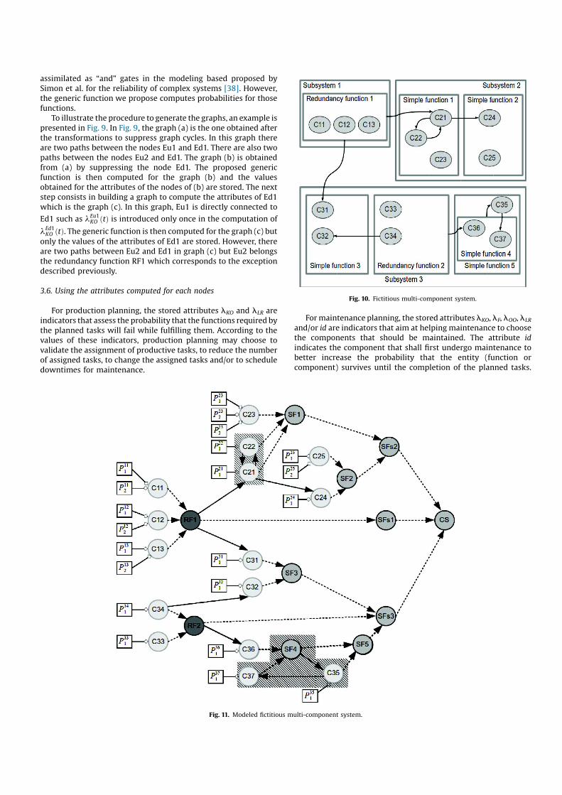
Fig. 10. Fictitious multi-component system.

Fig. 11. Modeled fictitious multi-component system.

If attributes lKO, of entities are beyond the maximum acceptable

probability of inability to fulfill the planned productive tasks, the

impact of the maintenance of the components, which are indicated

by the attributes id of those same entities, can be checked a priori.

This is can be done by setting, for example, to zero (or to a very low

value) the values of the local prognoses of the components that are

supposed to undergo maintenance and by running the proposed

generic function again with these new values of the local

prognostics. Afterward, the function will provide the new values

of the attributes lKO, lF, lOO, lLR and id for the new proposed

repairs if some attributes lKO still have too high values. The

discrepancies between the values of the attributes lKO, lF, lOO, lLR

before and after maintenance will so enable to assess the efficiency

of the maintenance of components relatively to the ability of the

entities (mainly functions) of the complex system to complete the

planned tasks.

Thanks to the proposed decision indicators, production

scheduling and maintenance management can jointly make the

best decision according to joint performance indicators [5,6,35].

The decision can be, but not limited to, to validate the assignment

of productive tasks, to reduce the number of assigned tasks, to

change the assigned tasks, to schedule downtimes and, for

downtimes, to choose the components to maintain.

4. Example of multi-component system and experimental

results

The aim of this part is to present the decision support indicators

the proposed generic function for complex system provides and

how this function could be used by production and maintenance

planning. These results are obtained from a fictitious multi-

component system whose goal is to bring together most of the

situations that may be encountered in complex systems from the

point of view of the proposed prognostic function computation.

The fictitious complex system, which is presented in Fig. 10, is

made of three subsystems that contains redundancy functions or

simple functions. Several components (Cx) implement the

functions. In Fig. 10, the arcs are the causal relationships of the

structural knowledge modeling.

This fictitious multi-component system is modeled according

to the behavioral, structural and functional knowledge modeling

principles described in this paper. The model of this fictitious

complex system is shown in Fig. 11 where Cx is for the component

number x, Pxi is the local prognostics number i of the component Cx,

RFk is the redundancy function number k, SFl is the simple function

number l, SFsj is the subsystem number j that is considered as a

simple functions and CS is the complex system.

Transforming the graph cycles, that the hatched areas highlight,

of the modeled fictitious complex system by using functions of

interdependence, the model of the fictitious complex system

becomes the one presented in Fig. 12 where SFim is the simple

function of interdependence number m. Then three graphs are

generated to avoid to introduce several times the probability of the

KO state of one node to the computation of the KO state of another

one unless it belongs to a redundancy function. These graphs are

presented in Figs. 13–15 on which the proposed generic is

successively run. The results computed for all the nodes of the

graph of Fig. 13 are stored. For the graph of Fig. 14, only the results

Fig. 12. Transformed model of the fictitious multi-component system to suppress graph cycles.

computed for the nodes SFs2 and SFs3 are stored and, for the graph

of Fig. 15, only the results computed for the node CS are stored. The

stored values of the attributes of nodes are decision support

indicators for production and maintenance scheduling.

Four scenarios whose results are presented in Table 1 have been

computed from the graphs of Figs. 13–15. In those scenarios, we

consider that the planned productive tasks will solicit all the

functions of the system and that their probability to fail before the

completion of those tasks must not be beyond 1.5e-2 and that the

only criterion to maintain components is the improvement of

reliability according to rules (13) and (14).

The scenario 1 consists of a situation where all the local

prognostics assess probabilities of failure before the end of

scheduled tasks assigned to the complex system at 1e-4.

The scenario 2 is based on the same situation as the scenario 1

but the local prognostics P121 and P251 provide assessed probabilities

of failure before the end of scheduled tasks assigned to the system

at 3e-2 and the local prognostics P112 , P211 , P341 and P371 provide

assessed probabilities of failure before the end of scheduled tasks

assigned to the system at 1e-2. Then two decisions can be made

according to the indicators provided by the proposed generic

function and presented in Table 1:

The production planning defines a new sequence of tasks for

which there is no function whose probability of failure before the

achievement of this sequence is greater than 1.5e-2, and

maintenance planning schedules the necessary actions on

components C25 and C37 after the completion of this sequence

thanks to the values of their local prognostics.

The production planning decides not to solicit the complex

system and maintenance of components C25 and C37 is

undertaken.

The scenario 3 is based on the same situation as the scenario 2

but the components whose identifiers appear in the attributes id of

the functions whose attributes lKO or lLR are greater than 1.5e-2

are maintained. These components are C25 and C37 highlighted in

dark grey in Table 1. To check if the maintenance of those two

components is enough to get under the maximum allowed

probability that a function of the system fails before the

Fig. 13. First graph generated to avoid to introduce several times the probability of the KO state of one node.

completion of the planned tasks, the local prognostics P251 , P252 and

P371 are set to 1e-6 assuming the maintenance of C25 and C37 is

done (but it could be other values much lower than the ones before

their maintenance). For this scenario, the proposed generic

function is successively run for the three graphs with those new

values of P251 , P252 and P371 . The indicators it provides suggests to

maintain C34 too, if production planning needs that the maximum

allowed probability of the complex system CS before the

completion of the planned tasks is 1.5e-2. Thus, three components

should undergo maintenance to get under the maximum allowed

probability of failure of a function before the end of the tasks

planned for the scenario 2. After the maintenance of C34, we

suppose P341 is set to 1e-6 too (but it could be another value much

lower than the one before its maintenance) and then the proposed

function is processed again for the three graphs. The provided

indicators show that if C25, C37 and C34 are maintained, there is no

more function whose probability of failure before the completion

of the planned tasks is greater than 1.5e-2 (the supposed

maximum allowed threshold). Indeed, in this case lCSKO is highest

value which is lower than 1.09e-2.

The scenario 4 highlights the ability of the proposed generic

function to predict propagations of failures and their effects on the

functioning of functions and subsystems. In this case the systems

must implement a diagnostic module. When a local diagnostic

states that a component is failed, at least one of its local

prognostics must be set to one (the value of the prognostic must

be saved in a buffer to be recovered if needed later). Then the

prognostic function is successively run from step 4 for the three

graphs. Then, each component or function whose attribute lKO is

equal to one can consequently be considered out of order. These

results can especially be used for the consistency based diagnosis

approach in order to reduce the number of candidate components

[2]. Indeed, the second stage of consistency based diagnostic

consists in verifying the candidates. If components or functions

that are prognosed “out of order” consequently to the failure of a

component are still operating according to their own diagnostic

modules, one can consider that the component that is the origin of

these prognostics is not failed and that it was due to a false

detection and so the local prognostic that was set to one must be

reset to the value that was saved in the buffer and the proposed

generic function is processed again for the three graphs. The

Fig. 14. Second graph generated to avoid to introduce several times the probability of the KO state of one node.

computed values of lKO and lLR can also be used by production

operators to make decision about how to adapt to the detected

failure. The scenario 4 is based on the scenario 3 but the

components C12 and C34 are diagnosed as failed. The conse-

quences are that functions SF3, SFs3 and CS are out of order and the

redundancy of RF2 is lost.

5. Conclusion

A generic function providing decision supports for production

and maintenance based on Bayesian networks to infer the ability

of complex system to complete planned tasks from local

prognostics and on an extension to identify components to be

maintained, was presented in this paper. The decision support

indicators it provides help the production planning to assign

productive tasks and also to guide maintenance toward the

components that should firstly be maintained. The implementa-

tion of this function requires a modeling of the system that

consists of graphs that represent functional, structural and a part

of the behavioral knowledge about the system. The method to

build those modeling graphs to adapt them to the generic

function requirements was presented. The inputs of this function

are the local prognostics of the components. These local

prognostics provide the probabilities that the components fail

according to their different failures modes before the end of the

tasks that production planning has assigned to the system. From

these local prognostics, the generic function assesses the values of

the transitions between the states of each node of the complex

system model and so it provides, for all the hierarchical levels, the

ability of functions and subsystems to fulfill the planned

productive tasks. These values are the probabilities that the

different entities of the complex systems (components, functions,

subsystems, etc.) fail or become out of order before the end of the

assigned tasks. These probabilities are decision support indicators

used by production planning to valid or not to valid the tasks

scheduling for a given complex system and they can be used to

define the downtimes of this given complex system to perform

maintenance. The proposed prognostic function also guides

maintenance toward the components that need it in order to

shorten downtimes by enabling to plan the maintenance actions

and their logistics in advance. Therefore the proposed generic

function contributes to a better compromise between the

satisfaction of the respective objectives of the condition based

maintenance and of the production planning. The proposed

prognostic function can predict propagations of failures and their

effects on the functioning of functions and subsystems and thus it

can be reused to implement a consistency based diagnostic

function dedicated to the system. In this case the diagnostic

function and the prognostic function can share a part of the system

modeling. Scenarios were described to show how the provided

decision support indicators can be used for production and

maintenance planning purposes.

Fig. 15. Third graph generated to avoid to introduce several times the probability of the KO state of one node.

Further developments of this work will deal with the

implementation of the prognostic function on a real system.

Other developments will aim at making interoperable various

uncertainty models used for the local prognoses. This could be

brought into operation thanks to the Dempster-Shafer evidence

theory or of the transferable belief model that includes a credal

level to represent and to combine the information and a pignistic

level for decision making [13,38–40].

Appendix A.

lCxKO tð Þ ¼ 1 # 1 # l

CxF tð Þ

!

1 # lCxOO tð Þ

!

lCxKO tð Þ ¼ 1 # 1 # lCx

F tð Þ !

1 # 1 # PEi2G

#1Cxð Þ

1 # lEiKO tð Þ

!h in o

lCxKO tð Þ ¼ 1 # 1 # lCx

F tð Þ !

:PEi2G

#1Cxð Þ

1 # lEiKO tð Þ

!

If a node E is a simple function, then lEF tð Þ ¼ 0, hence:

lCxKO tð Þ ¼ 1

# 1 # lCxF tð Þ

!

:PEi2G

#1Cxð Þ

1 # 1 # 1 # lEiF tð Þ

!

1 # lEiOO tð Þ

!h in o

lCxKO tð Þ ¼ 1 # 1 # lCx

F tð Þ !

:PEi2G

#1Cxð Þ

1 # lEiF tð Þ

!

1 # lEiOO tð Þ

!h i

lCxKO tð Þ ¼ 1 # 1 # lCx

F tð Þ !

:PEi2G

#1Cxð Þ

1 # lEiF tð Þ

!

1 # 1 # PEj2G

#1Eið Þ

1 # lEjKO tð Þ

!h ih in o

lCxKO tð Þ ¼ 1 # 1 # lCx

F tð Þ !

:PEi2G

#1Cxð Þ

1 # lEiF tð Þ

!

:PEj2G

#1Eið Þ

1 # lEjKO tð Þ

!n o

If we note A#1 Eð Þ the set of the nodes, from which the node E is

attainable, we then recursively obtain:

lCxKO tð Þ ¼ 1 # 1 # lCx

F tð Þ !

:PEk2A#1 Cxð Þ

1 # lEkF tð Þ

!

Hence, the value lEmF tð Þ 2%0; 1%, if it was zero, would decrease at

most lCxKO tð Þ is such as:

lEmF tð Þ ¼ max lCx

F tð Þ; maxEk2A#1 Cxð Þ

lEkF tð Þ

!

!

References

[1] A. Arnaiz, S. Ferreiro, M. Buderath, New decision support system based onoperational risk assessment to improve aircraft operability, Proc. Inst. Mech.Eng. Part O J. Risk Reliab. 224 (2010) 137–147.

[2] J. Biteus, M. Nybergb, E. Friska, An algorithm for computing the diagnoses withminimal cardinality in a distributed system, Eng. Appl. Artif. Intell. 21 (2008)269–276.

[3] M. Blaha, J. Rumbaugh, Object Oriented Modeling and Design with UML, 2nded., Pearson Prentice-Hall, Chesterfield, 2005.

[4] C. Byington, M. Watson, M. Roemer, T. Galie, Prognostic enhancements to gasturbine diagnostic systems, Proceedings of the IEEE Aerospace Conference, BigSky, USA, 2001.

[5] M. Chaouqi, J. Benhra, A. Zakari, Agile approach for joint scheduling ofproduction and maintenance in flow shop, Int. J. Comput. Appl. 59 (2012) 29–36.

[6] T. Coudert, B. Grabot, B. Archimède, Production/maintenance co-operativescheduling using multi-agents and fuzzy logic, Int. J. Prod. Res. 40 (2002) 4611–4632.

[7] J. Dunjo, V. Fthenakis, J.A. Vilchez, J. Arnaldos, Hazard and operability (HAZOP)analysis. A literature review, J. Hazard. Mater. 173 (2010) 19–32.

[8] W. Elghazel, J. Bahi, C. Guyeux, M. Hakem, K. Medjaher, N. Zerhouni,Dependability of wireless sensor networks for industrial prognostics andhealth management, Comput. Ind. 68 (2015) 1–15.

Table 1

Results of the computed scenarios for the fictitious multi-component system.

Scenario 1 Scenario 2 Scenario 3 Scenario 4

Node id lLR lKO id lLR lKO id lLR lKO id lLR lKO id

CS 1.40E # 03 C23 5.98E # 02 C25 2.08E # 02 C34 1.00E + 00 C34

SFi2 3.00E # 04 C22 1.02E # 02 C37 2.02E # 04 C35 3.01E # 04 C35

SFi1 2.00E # 04 C21 1.01E # 02 C21 1.01E # 02 C21 1.01E # 02 C21

SFs3 6.00E # 04 C35 2.03E # 02 C37 1.04E # 02 C34 1.00E + 00 C34

SFs2 8.00E # 04 C23 4.03E # 02 C25 1.05E # 02 C21 1.05E # 02 C21

SFs1 8.00E # 12 C13 6.08E # 08 C12 6.08E # 08 C12 2.02E # 06 C12

SF5 3.00E # 04 C35 1.02E # 02 C37 2.02E # 04 C35 3.01E # 04 C35

SF4 3.00E # 04 C35 1.02E # 02 C37 2.02E # 04 C35 3.01E # 04 C35

SF3 3.00E # 04 C32 1.02E # 02 C34 1.02E # 02 C34 1.00E + 00 C34

SF2 5.00E # 04 C25 4.00E # 02 C25 1.02E # 02 C21 1.02E # 02 C21

SF1 5.00E # 04 C23 1.04E # 02 C21 1.04E # 02 C21 1.04E # 02 C21

RF2 2.00E # 04 1.00E # 08 C33 1.01E # 02 1.00E # 06 C34 1.01E # 02 1.00E # 06 C34 1.00E + 00 1.00E # 04 C34

RF1 1.20E # 07 8.00E # 12 C13 3.12E # 04 6.08E # 08 C12 3.12E # 04 6.08E # 08 C13 1.03E-02 2.02E # 06 C12

C37 1.00E # 04 C37 1.00E # 02 C37 1.00E # 06 C37 1.00E # 06 C37

C36 1.00E # 04 C36 1.01E # 04 C36 1.01E # 04 C36 2.00E # 04 C36

C35 1.00E # 04 C35 1.00E # 04 C35 1.00E # 04 C35 2.00E # 04 C35

C34 1.00E # 04 C34 1.00E # 02 C34 1.00E # 02 C34 1.00E + 00 C34

C33 1.00E # 04 C33 1.00E # 04 C33 1.00E # 04 C33 1.00E-04 C33

C32 2.00E # 04 C32 1.01E # 02 C34 1.01E # 02 C34 1.00E + 00 C34

C31 1.00E # 04 C31 1.00E # 04 C31 1.00E # 04 C31 1.02E # 04 C31

C25 2.00E # 04 C25 3.01E # 02 C25 2.00E # 06 C25 2.00E # 06 C25

C24 3.00E # 04 C24 1.02E # 02 C21 1.02E # 02 C21 1.02E # 02 C21

C23 3.00E # 04 C23 3.00E # 04 C23 3.00E # 04 C23 3.00E # 04 C23

C22 1.00E # 04 C22 1.00E # 04 C22 1.00E # 04 C22 1.00E # 04 C22

C21 1.00E # 04 C21 1.00E # 02 C21 1.00E # 02 C21 1.00E # 02 C21

C13 2.00E # 04 C13 2.00E # 04 C13 2.00E # 04 C13 2.00E # 04 C13

C12 2.00E # 04 C12 3.01E # 02 C12 3.01E # 02 C12 1.00E + 00 C12

C11 2.00E # 04 C11 1.01E # 02 C11 1.01E # 02 C11 1.01E # 02 C11

[9] Q. Feng, Y. Chen, B. Sun, S. Li, An optimization method for conditionbased maintenance of aircraft fleet considering prognostics uncertainty, Sci.World J. 2014 (2014), doi:http://dx.doi.org/10.1155/2014/430190 (Article ID430190).

[10] S. Ferreiro, A. Arnaiz, B. Sierra, I. Irigoien, Application of Bayesian networks inprognostics for a new integrated vehicle health management concept, ExpertSyst. Appl. 39 (2012) 6402–6418.

[11] P. Goupil, AIRBUS state of the art and practices on FDI and FTC in flight controlsystem, Control Eng. Pract. 19 (2011) 524–539.

[12] R. Gouriveau, N. Zerhouni, Connexionist-systems-based long term predictionapproaches for prognostics, IEEE Trans. Reliab. 61 (2012) 909–920.

[13] W. He, N. Williard, M. Osterman, M. Pecht, Prognostics of lithium-ion batteriesbased on Dempster–Shafer theory and the Bayesian Monte Carlo method, J.Power Sources 196 (2011) 10314–10321.

[14] A. Heng, A.C.C. Tan, J. Mathew, N. Montgomery, D. Banjevic, A.K.S. Jardine,Intelligent condition-based prediction of machinery reliability, Mech. Syst. Sig.Process. 23 (2009) 1600–1614.

[15] W. Hong-Feng, Prognostics and Health Management for complex system basedon fusion of model-based approach and data-driven approach, Phys. Procedia24 (2012) 828–831.

[16] B. Iung, M. Monnin, A. Voisin, P. Cocheteux, E. Levrat, Degradation state model-based prognosis for proactively maintaining product performance, CIRP Ann.Manuf. Technol. 57 (2008) 49–52.

[17] G. Jacazio, M. Sorli, D. Bolognese, D. Ferrara, Health management system forthe pantographs of tilting trains, Proceedings of First European Conference ofthe Prognostics and Health Management Society, Dresden, Germany, 2012, pp.127–140 (July 3–5).

[18] A.K.S. Jardine, D. Lin, D. Banjevic, A review on machinery diagnostics andprognostics implementing condition-based maintenance, Mech. Syst. Sig.Process. 20 (2006) 1483–1510.

[19] G. Jin, D.E. Matthews, Z. Zhou, A Bayesian framework for on-line degradationassessment and residual life prediction of secondary batteries in spacecraft,Reliab. Eng. Syst. Saf. 113 (2013) 7–20.

[20] N. Julka, A. Thirunavukkarasu, P. Lendermann, B.P. Gan, A. Schirrmann, H.Fromm, E. Wong, Making use of prognostics health management informationfor aerospace spare components logistics network optimization, Comput. Ind.62 (2011) 613–622.

[21] T. Koski, J.M. Noble, Bayesian Networks: an Introduction, John Wiley & SonsInc., Chichester, 2009.

[22] A. Kossiakoff, W.N. Sweet, S. Seymour, S.M. Biemer, Systems EngineeringPrinciples and Practice, 2nd ed., John Wiley & Sons Inc., Hoboken, 2011.

[23] K. Le Son, M. Fouladirad, A. Barros, E. Levrat, B. Iung, Remaining useful lifeestimation based on stochastic deterioration models: a comparative study,Reliab. Eng. Syst. Saf. 112 (2013) 165–175.

[24] J. Lee, J. Ni, D. Djurdjanovic, H. Qiu, H. Liao, Intelligent prognostics tools and e-maintenance, Comput. Ind. 57 (2006) 476–489.

[25] Q. Liu, M. Dong, W. Lv, X. Genga, Y. Li, A novel method using adaptive hiddensemi-Markov model for multi-sensor monitoring equipment health prognosis,Mech. Syst. Sig. Process. 64–65 (2015) 217–232.

[26] G. Medina-Oliva, P. Weber, B. Iung, PRM-based patterns for knowledgeformalisation of industrial systems to support maintenance strategiesassessment, Reliab. Eng. Syst. Saf. 116 (2013) 38–56.

[27] G. Medina-Oliva, P. Weber, B. Iung, Industrial system knowledge formalizationto aid decision making in maintenance strategies assessment, Eng. Appl. Artif.Intell. 37 (2015) 343–360.

[28] K. Medjaher, D.A. Tobon-Mejia, N. Zerhouni, Remaining useful life estimationof critical components with application to bearings, IEEE Trans. Reliab. 61(2012) 292–302.

[29] A. Muller, M.C. Suhner, B. Iung, Formalisation of a new prognosis model forsupporting proactive maintenance implementation on industrial system,Reliab. Eng. Syst. Saf. 93 (2008) 234–253.

[30] K.A. Nguyen, P. Do, A. Grall, Multi-level predictive maintenance for multi-component systems, Reliab. Eng. Syst. Saf. 144 (2015) 83–94.

[31] L. Rémy, A. Alam, N. Haddar, A. Köster, N. Marchal, Growth of small cracks andprediction of lifetime in high-temperature alloys, Mater. Sci. Eng. A 468–470(2007) 40–50.

[32] S. Sankararaman, M.J. Daigle, K. Goebel, Uncertainty quantification inremaining useful life prediction using first-order reliability methods, IEEETrans. Reliab. 63 (2014) 603–619.

[33] S. Sankararaman, Y. Ling, S. Mahadevan, Uncertainty quantification and modelvalidation of fatigue crack growth prediction, Eng. Fract. Mech. 78 (2011)1487–1504.

[34] A. Saxena, J. Celaya, B. Saha, S. Saha, K. Goebel, Metrics for offline evaluation ofprognostic performance, Int. J. Prognostics Health Manage. 1 (2010) 1–20.

[35] E. Sanmarti, A. Espufia, L. Puigjaner, Batch production and preventivemaintenance scheduling under equipment failure uncertainty, Comput.Chem. Eng. 21 (1997) 1157–1158.

[36] P. Scarf, A Framework for condition monitoring and condition basedmaintenance, Qual. Technol. Quant. Manage. 4 (2007) 301–312.

[37] E.L. Silva Teixeira, B. Tjahjono, S.C. Absi Alfaro, A novel framework to linkprognostics and health management and product-service systems usingonline simulation, Comput. Ind. 63 (2012) 669–679.

[38] C. Simon, P. Weber, E. Levrat, Bayesian networks and evidence theory to modelcomplex systems reliability, J. Comput. 2 (2007) 33–43.

[39] C. Simon, P. Weber, A. Evsukoff, Bayesian networks inference algorithm toimplement Dempster Shafer theory in reliability analysis, Reliab. Eng. Syst. Saf.93 (2008) 950–963.

[40] P. Smets, R. Kennes, The transferable belief model, Artif. Intell. 66 (1994) 191–234.

[41] R. Sweeney, Achieving Service-Oriented Architecture: Applying an EnterpriseArchitecture Approach, John Wiley & Sons Inc., Hoboken, 2010.

[42] R.E. Tarjan, Depth-first search and linear graph algorithms, SIAM J. Comput. 1(1972) 146–160, doi:http://dx.doi.org/10.1137/0201010.

[43] D.A. Tobon-Mejia, K. Medjaher, N. Zerhouni, G. Tripot, A data-driven failureprognostics method based on mixture of Gaussians hidden Markov models,IEEE Trans. Reliab. 61 (2012) 491–503.

[44] G. Vachtsevanos, F.L. Lewis, M. Roemer, A. Hess, B. Wu, Intelligent FaultDiagnosis and Prognosis for Engineering System, John Wiley & Sons Inc.,Hoboken, 2006.

[45] A. Voisin, E. Levrat, P. Cocheteux, B. Iung, Generic prognosis model forproactive maintenance decision support: application to pre-industrial e-maintenance test bed, J. Intell. Manuf. 21 (2010) 177–193.

[46] P. Weber, L. Jouffe, Complex system reliability modelling with dynamic ObjectOriented Bayesian Networks (DOOBN), Reliab. Eng. Syst. Saf. 91 (2006) 149–162.

[47] H. Worn, T. Langle, M. Albert, A. Kazi, A. Brighenti, S. Revuelta Seijo, Diamond:distributed multi-agent architecture for monitoring and diagnosis, Prod.Plann. Control 15 (2004) 189–200.

[48] R.C.M. Yam, P.W. Tse, L. Li, P. Tu, Intelligent predictive decision support systemfor condition-based maintenance, Int. J. Adv. Manuf. Technol. 17 (2001) 383–391.

[49] F. Zhao, Z. Tian, Y. Zeng, Uncertainty quantification in gear remaining useful lifeprediction through an integrated prognostics method, IEEE Trans. Reliab. 62(2013) 146–159.

[50] E. Zio, Reliability engineering: old problems and new challenges, Reliab. Eng.Syst. Saf. 94 (2009) 125–141.